rising groundwater levels associated with sea level … · 2015-03-25 · ipwea wa state conference...
TRANSCRIPT

IPWEA WA STATE CONFERENCE MARCH 2015
J5853a 27 January 2015 1
RISING GROUNDWATER LEVELS ASSOCIATED WITH SEA LEVEL RISE
Barnett, J.C., Rogers, A.D., Serafini, G., Davies, J.R.
JDA Consultant Hydrologists Subiaco Western Australia
1. Introduction
Global sea-levels are rising. As Shakespeare put it: “…. I have seen the hungry Ocean gain
advantage on the kingdom of the shore”.
State Planning Policy 2.6 State Coastal Planning incorporates the report: “Sea Level Change
in Western Australia: Application to Coastal Planning”. This report, dated February 2010,
gives a comprehensive summary of historical sea-level change and its causes, and
recommends that: “a vertical sea level rise of 0.9m be adopted when considering the setback
difference and elevation to allow for the impact of coastal processes over a 100 year planning
timeframe (2010 to 2110)”.
One of the consequences of sea-level rise will be a corresponding rise in groundwater levels
near the coast, as groundwater discharge adjusts to the higher base level of the ocean and
rivers.
This will happen in many coastal areas around the world. Perth and the Swan Coastal Plain in
general (particularly between Perth and Busselton) will be adversely affected, having a highly
permeable aquifer adjacent to the coast, and a shallow water-table.
In terms of the Conference theme “Solutions Beyond Boundaries” this paper addresses the
need for all levels of government to address the inevitable groundwater rise associated with
sea-level rise, hence “moving the boundary” of community concerns from the ocean side of
the coast (sea-level rise) to the landward side (groundwater rise).
2. Sea-Level Trends
Sea-levels have fluctuated widely throughout geological time. In the last 140,000 years
they have risen and fallen many times as polar icecaps have advanced and retreated. If
you had stood on the Darling Scarp 20,000 years ago, and looked to the west, the ocean
would have been out of sight, well beyond the horizon. Since that time, not a long time
geologically speaking, sea-levels have risen by about 140m. In the last 5000 years levels
have been quite stable, but in the 15,000 years before that they rose so rapidly that
aborigines living on the coastal plain would have noticed the ocean advancing during a
lifetime.
About 110,000 years ago, in the last interglacial, sea-levels are thought to have been 5
to 8m higher than the present day.
Over shorter time-periods, it can be difficult to distinguish between variations in sea level
and longer-term trends in Mean Sea Level, particularly as many of the variations are of
much greater amplitude than any underlying trend.
Mean Sea Level (MSL) is defined as the height of the sea relative to a local land benchmark,
averaged over a period of time, such as a month or a year, so that fluctuations caused by
waves or tides are largely removed (UNESCO, 2002).
As measured by coastal tide gauges, MSL is therefore relative to any movement of the
land that affects the benchmark, and any trend may be caused either by movement of
the land or by actual change in the adjacent sea surface. Measured changes in sea-level
must therefore be corrected for land movements to determine any absolute change in
MSL. Such land movements i n c l u d e isostatic changes caused by long-term adjustment
of continental plates to large-scale deposition and erosion of sediment, t o advance and
retreat of icecaps, groundwater abstraction, or indeed to large changes in sea-level. Major
earthquakes are another potential influence.
Many other factors also affect sea-level, including storm surges, tsunamis, changes in
water density as a result of temperature changes, and ocean currents. Barometric pressure
also affects sea-levels, low pressure causing a rise, high pressure a fall.
The El Nino Southern Oscillation (ENSO) affects both climate and sea-levels around

IPWEA WA STATE CONFERENCE MARCH 2015
J5853a 27 January 2015 2
Australia. ENSO alternates between El Nino and La Nina conditions in a three to eight
year cycle (BoM, 2005). El Nino is characterised by warmer temperatures in the central to
eastern Pacific Oc ean and lower than normal sea-levels (Haigh et al, 2011), and may
cause drought, particularly in eastern Australia. La Nina has the opposite effect, causing
cooler than normal ocean temperatures in the eastern Pacific, higher than normal sea-
levels and higher than average rainfall in the north and east of Australia.
The main control on global sea-level over the longer term is the net loss or gain of ice in
the polar regions.
In Antarctica, conditions are not uniform, but there appears to be a general net loss, with
decrease of ice mass on land exceeding an increase of sea ice (Hambrey et al, 2010). The
East Antarctic ice-sheet is approximately stable, with ice loss balanced by increased
snowfall. This is just as well, as melting of this ice sheet would cause a rise in global sea-
level of about 60m! West Antarctica shows a net loss of ice, contributing an estimated
0.3mm/year rise in sea-level, with potential total loss of 3.3m. The Antarctic Peninsula is
also losing ice, but not at a rate which is likely to noticeably affect sea-levels.
In the Arctic, as we have seen on the news over the past few years, the ocean is losing
more and more of its ice cover in summer, and may be completely ice free in summer
within 40 years if current trends continue. The North West Passage opened for the first
time in human memory in 2007 and did so again in 2012. The melting of floating ice,
however, although spectacular in recent years, does not contribute to sea-level rise. The
Greenland icesheet is a different matter, where net ice loss is estimated to be adding
about 1.3mm/year to global sea-levels, with an increasing trend and potential total rise
of 7m.
Glaciologists in general forecast an aggregate contribution of about 1m to sealevel rise
by 2100, with some predicting up to 2m.
Recent studies have suggested that worldwide abstraction of groundwater may be
contributing about 0.4mm/year to sea-level rise (Konikow, 2011), and may be contributing
0.8mm/year by 2050 (Wada et al, 2012). This would be due to increased evaporation and
consequent increased rainfall, and to runoff into canals and rivers.
Sea-levels have been measured precisely in Australia since the early 1990's by the
Australian Baseline Sea-Level Monitoring Project. This uses an array of 16 tidal gauges,
termed S E A F R A M E stations (UNESCO, 2002). SEAFRAME stands for Sea-level Fine
Resolution Acoustic Measuring Equipment. One of these is at Hillarys. These stations have
been supplemented by satellite imagery since the 1990's, TOPEX/Poseidon (launched 1992),
Jason-1 (launched 2001) and Jason-2 (launched 2008). The SEAFRAME and satellite
measurements show good agreement.
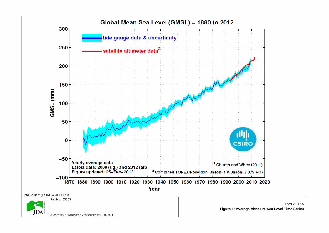
Current CSIRO estimates indicate that, after several thousand years of relative stability,
sea-levels apparently started rising slowly from about 1870, with increasing rates from
about 1940 and again in the early 1990's (Figure 1). The rate of rise has averaged about
1.7mm/year since 1870, and 3.2mm/year since the early 1990's (CSIRO/ACERC, 2014).
The Intergovernmental Panel on Climate Change (IPCC) predicts a total rise of between
0.5m and 0.95m by 2100, with a mean value estimate of 0.73 (IPCC, 2014).
The Western Australian Planning Guideline of 0.9m is therefore a prudently conservative
value, according to the current knowledge of sea-level controls and trends.
3. UNSW – Water Research Laboratory Study
A UNSW – Water Research Laboratory Study (2013) concluded that water-table response
to sea level rise was most significant in coastal aquifers with high transmissivity and low
hydraulic gradient.
Their modelling confirmed that the water-table rise would match sea-level rise near the
coast, and diminish further inland. T h e S t u d y n o t ed t h a t s uch a rise in water-table
near the coast may affect sewers and the basements of buildings, and may affect the
stability of swimming pools and underground tanks.
The UNSW-WRL Study also indicated that the seawater interface in a coastal aquifer

IPWEA WA STATE CONFERENCE MARCH 2015
J5853a 27 January 2015 3
may intrude up to 1km further inland in response to a 1 m sea-level rise. This might
cause shallow bores near the coast to become brackish or saline.
A rise in sea-level may a l s o cause landward advance of the shoreline. Depending on
topography, a sea-level rise of lm may be expected to cause a shoreline advance in the
range 50 to 100m.
4. Groundwater Model
JDA has developed a groundwater model using MODFLOW to simulate the likely effect of a
h y p o t h e t i c a l l m sea-level rise on the water table by 2113 on a crosssection across
the Gnangara Mound (Figure 2). Modflow is an industry standard finite difference
numerical model for the simulation of groundwater.
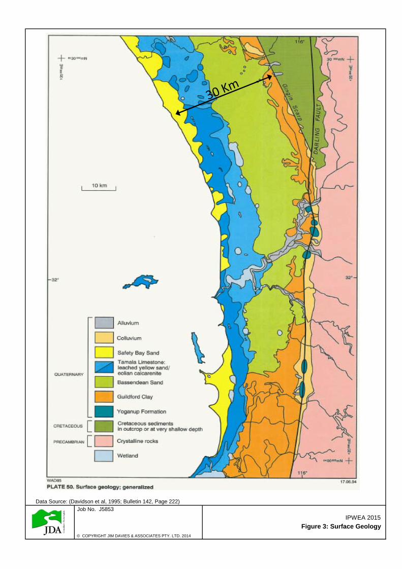
The surface geology in this area, across the coastal plain from west to east, consists of
the Safety Bay Sand, Tamala Limestone, Bassendean Sand and Guildford Formation (Figure
3). These form a single groundwater flow system, termed the superficial aquifer.
The two main components of this aquifer are the Tamala Limestone and the Bassendean
Sand (Figure 4). The Tamala Limestone consists of limestone and sand, the former
containing cavities and solution channels. It is highly permeable, with hydraulic
conductivity ranging from 100-10,000m/day, generally increasing towards the west. The
Bassendean Sand consists mostly of medium-grained moderately sorted sand, with much
lower hydraulic conductivity than the Tamala Limestone, about 10-15m/day.
Regional groundwater flow across the northern Gnangara Mound is a simple pattern of
flow from east to slightly south of west, to discharge into the Indian Ocean.
MODFLOW was used to create a vertical slice model, representing a cross-section across the
northern part of the Gnangara Mound, extending 30km inland, incorporating values of
hydraulic conductivity for the superficial aquifer from Davidson (1995). Recharge is
applied uniformly at 25 percent of average annual rainfall of 800mm. The model does not
include any interaction with surface watercourses, nor groundwater abstraction by bores
and wells.
The model was initially run in steady state mode to reproduce the present-day
configuration of the water-table across the Gnangara Mound. It was then run in transient
mode to simulate an annual rise of 10mm/year for 100 years for a total rise of 1m.
The representative cross-section for the year 2113 shown on Figure 5 shows a rise in water-
table at the coast of 1m, corresponding to the total sea-level rise, declining progressively
to 0.75m rise at 1km inland, 0.5m at 3.25km and 0.25m at 8.5km inland. At the top of
the Gnangara Mound the rise is predicted to be only 0.1m.
The JDA groundwater model thus provides a semi-quantitative estimate of water-table
rise in the superficial aquifer, in response to a 1m rise in sea-level by 2113. The model
provides a basis for future development which could take account of local variations in
hydrogeology and transmissivity.
The predicted groundwater rise across the model domain shows a marked decrease where
the water-table passes from the highly transmissive Tamala limestone adjacent to the
coast into the much less transmissive Bassendean sand further inland, as shown
schematically on Figure 6.
Davidson (1995) includes a map proving transmissivity contours in the superficial aquifer,
reproduced here as Figure 7. The water-table predicted by the JDA groundwater model
can be extrapolated over the Perth coastal region by correlation with variations in
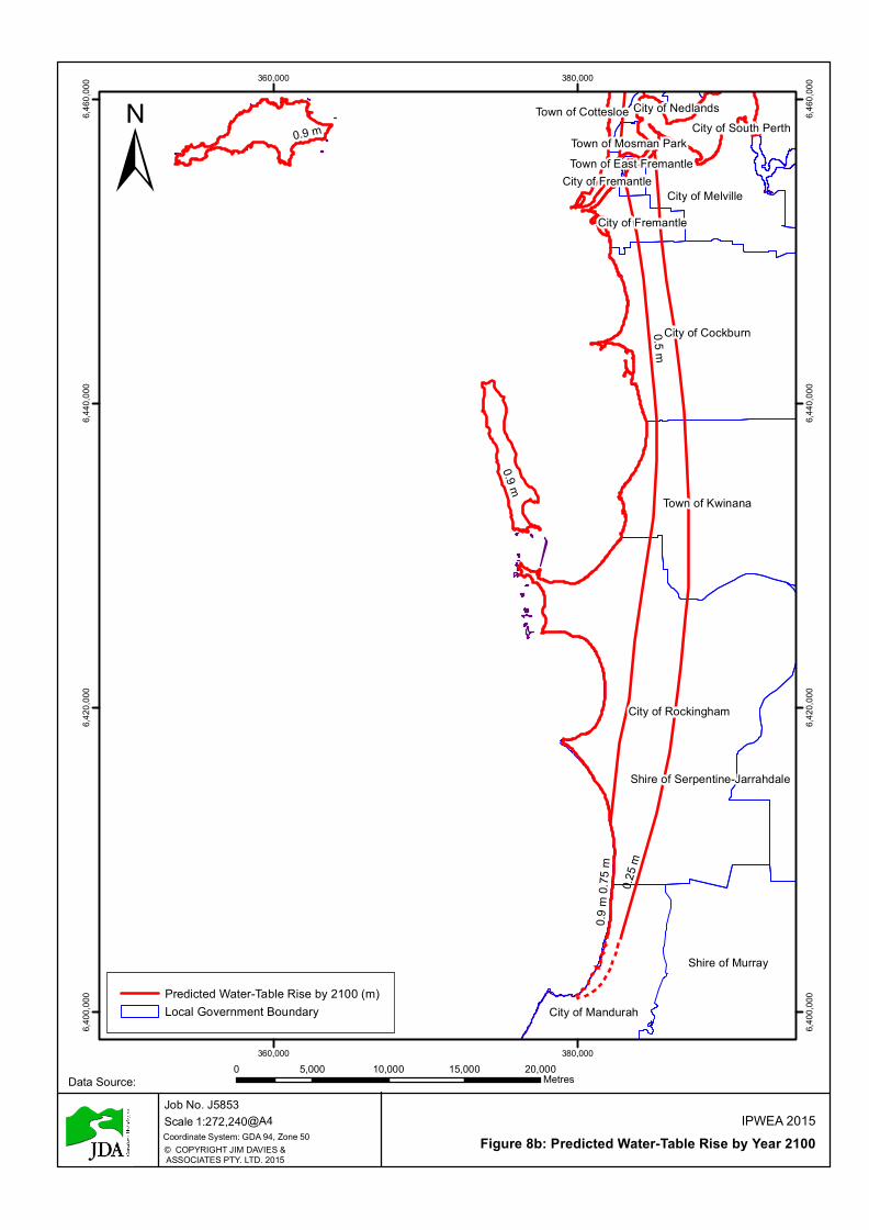
transmissivity (Figures 8a and 8b). Sea level rise will be transferred upstream in the
Swan River causing a groundwater rise along the river foreshore. Transmissivity is
generally relatively low inland along the river, however, so that the water-table rise will
not progress far from the shore.
The extent of water-table rise will therefore vary across different council boundaries,
according to local variations in the geology and superficial aquifer transmissivity. In
general to the north of the Swan River (Figure 8a) Wanneroo, Joondalup, Stirling and the
western suburbs will be the most affected coastlines, and to the south of Perth (Figure

IPWEA WA STATE CONFERENCE MARCH 2015
J5853a 27 January 2015 4
8b) Fremantle, Cockburn, Kwinana, Rockingham and Mandurah. Further south Bunbury
and Busselton will experience similar rise.
Where the water table is already shallow, obviously the effect of groundwater rise will be to
reduce the separation between ground surface and the water table.
5. Conclusions
The present Western Australian Planning Guideline of a 0.9m rise in sea-level by 2100 is a
prudently conservative value.
Groundwater levels in Perth will rise in response to sea-level rise. A rise of 0.9m in sea-level
will cause an equivalent rise in the water-table adjacent to the coastline, diminishing
progressively inland. The water-table rise will decrease markedly where it passes from the
highly transmissive Tamala Limestone near the coast into the much less transmissive
Bassendean Sand further inland.
The water-table rise will decrease the separation between land surface and groundwater
(even in areas with groundwater controls such as subsoil drainage) and may affect sewer
systems, basements of buildings, and the stability of swimming pools and underground tanks.
Sea-level rise is also likely to cause the salt water interface in the superficial aquifer to migrate
inland, perhaps by as much as 1km, causing some bores near the coast to become brackish.
A 0.9m sea-level rise may also cause landward encroachment by the ocean, by up to 100m,
depending on local topography.
Management of the effects of water-table rise will require improved monitoring of water-table
levels, and of the saltwater interface in the superficial aquifer, in coastal suburbs.
The effect of this inevitable rise in water table needs to be factored into policy settings at all
levels of government and to be integral to future land use planning.
Within our children’s lifetimes we will indeed see “the hungry Ocean gain advantage on the
kingdom of the shore”.
6. References
Bureau of Meteorology, 2005. El Nino, La Nina and Australia’s Climate.
www.bom.gov.au/info/leaflets.nino-nina.pdf
CSIRO and ACERC (2014). Sea Level Rise: Understanding the past – improving projections
for the future. www.cmar.csiro.au/sealevel/sl_impacts_sea_level.html
Davidson, W.A. (1995). Bulletin 142: Hydrogeology and groundwater resources of the Perth
region, Western Australia. Geological Survey of Western Australia.
Haigh, I.D., Eliot. M., Pattiarachi, C., Wahl, T. (2011). Regional changes in mean sea level
around Western Australia between 1897 and 2008, in: Coasts and Ports 2011: Diverse and
Developing: Proceedings of the 20th Australasian Coastal and Ocean Engineering Conference
and the 13th Australasian Port and Harbour Conference , Barton ACT, Engineers Australia
2011.
Hambrey, M., Bamber, J., Christoffersen, P., Glasser, N., Hubbard, A., Hubbard, B., Larter,
R., (2010) Glaciers: no-nonsense science, Geoscientist, Vol 20, No. 6.
IPCC (2014) Fifth Assessment Synthesis Report.
Konikow, L.F. (2011) Contribution of global groundwater depletion since 1900 to sea-level
rise. Geophysical Research Letters, Vol 38.
State Planning Policy 2.6 State Coastal Planning: Sea Level Change in Western Australia:
application to coastal planning, 2010. Department of Transport, Coastal Infrastructure,
Coastal Engineering Group.
UNESCO (2002) Manual on Sea Level Measurement and Interpretation, Volume III.
UNSW, Water Research Laboratory, 2013. Potential impacts of sea-level rise and climate
change on coastal aquifers.
www.connectedwaters.unsw.edu.au/resources/articles/coastal_aquifers.html
Wada, Y., van Beek, L.P.H., Sperna Weiland, F.C., Chao, B.F., Wu, Y-H., Bierkens, M.F.P.
Geophysical Research Letters, VR39.

Figures
IPWEA Conference 2015
Data Source: (CSIRO & ACECRC)
© COPYRIGHT JIM DAVIES & ASSOCIATES PTY. LTD. 2014
Job No. J5853IPWEA 2015
Figure 1: Average Absolute Sea Level Time Series

Data Source: (Davidson et al, 1995; Bulletin 142, Page 55)
© COPYRIGHT JIM DAVIES & ASSOCIATES PTY. LTD. 2014
Figure 2: Superficial Aquifer Flownet
Job No. J5853IPWEA 2015
Data Source: (Davidson et al, 1995; Bulletin 142, Page 222)
© COPYRIGHT JIM DAVIES & ASSOCIATES PTY. LTD. 2014
Job No. J5853IPWEA 2015
Figure 3: Surface Geology

Data Source: (Davidson et al, 1995; Bulletin 142, Page 48)
© COPYRIGHT JIM DAVIES & ASSOCIATES PTY. LTD. 2014
Figure 4: Gnangara Mound Geological Profile
Job No. J5853IPWEA 2015

Data Source:
© COPYRIGHT JIM DAVIES & ASSOCIATES PTY. LTD. 2014
Job No. J5853IPWEA 2015
Figure 5: Rise in Water-Table Along Modelled Transect
0.75 m Rise 1 km from coast
0.50 m Rise 3.25 km from coast
0.25 m Rise 8.5 km from coast

Data Source:
© COPYRIGHT JIM DAVIES & ASSOCIATES PTY. LTD. 2014
Job No. J5853IPWEA 2015
Figure 6: Conceptual Cross-Section Showing Water-Table Rise in High and Low Transmissivity Aquifers Along Shorelines
Natural Surface High Transmissivity Low Transmissivity
Inland extent of water‐table rise
Inland extent of water‐table rise
0.9m Sea level rise
Natural surface
Year 2110
Year 2015
Year 2110
Year 2015
Year 2015 Sea level
Year 2110 Sea level
Ocean
High transmissivity
Low transmissivity

Data Source: (Davidson et al, 1995; Bulletin 142, Plate 55)
© COPYRIGHT JIM DAVIES & ASSOCIATES PTY. LTD. 2014
Job No. J5853IPWEA 2015
Figure 7: Transmissivity Contours, Superficial Aquifer

0.9 m
0.75
m
City of Wanneroo
City of Swan
City of Stirling
City of Joondalup
Shire of Chittering
City of Melville City of Canning
City of Bayswater
City of Nedlands
Town of Cambridge
City of South Perth
City of Perth
Town of Victoria Park
City of Fremantle
Town of Vincent
City of Subiaco
Town of ClaremontTown of Cottesloe
Town of Mosman Park
City of FremantleTown of East Fremantle
City of Gosnells
City of Perth
0.5 m 0.25 m0.75 m
0.9 m
360,000
360,000
380,000
380,000
6,460
,000
6,460
,000
6,480
,000
6,480
,000
6,500
,000
6,500
,000
0 5,000 10,000 15,000 20,000Metres
Predicted Water-Table Rise by 2100 (m)Local Government Boundary
Job No. J5853IPWEA 2015
Figure 8a: Predicted Water-Table Rise by Year 2100
Data Source:
© COPYRIGHT JIM DAVIES & ASSOCIATES PTY. LTD. 2015
Scale 1:272,240@A4Coordinate System: GDA 94, Zone 50
0.9 m
0.75
m
City of Rockingham
City of Cockburn
Town of Kwinana
Shire of Murray
City of Melville
City of Mandurah
Shire of Serpentine-Jarrahdale
City of Fremantle
City of South PerthCity of Nedlands
Town of Mosman Park
City of Fremantle
Town of Cottesloe
Town of East Fremantle
0.5 m
0.25 m
0.9 m
0.9 m
360,000
360,000
380,000
380,000
6,400
,000
6,400
,000
6,420
,000
6,420
,000
6,440
,000
6,440
,000
6,460
,000
6,460
,000
0 5,000 10,000 15,000 20,000Metres
Predicted Water-Table Rise by 2100 (m)Local Government Boundary
Job No. J5853IPWEA 2015
Figure 8b: Predicted Water-Table Rise by Year 2100
Data Source:
© COPYRIGHT JIM DAVIES & ASSOCIATES PTY. LTD. 2015
Scale 1:272,240@A4Coordinate System: GDA 94, Zone 50