rilem technical committee - fenixeducristina/rrest/aulas_apresentacoes...materials and structures...

Materials and Structures (2006) 39:955-990DOI 10.1617/s11527-006-9193-x

RILEM TECHNICAL COMMITTEE

Round-Robin Test on methods ror determining chloridetransport parameters in concrete

M. Castellote • c. Andrade

Published online: 17 October 2006©RILEM 2006

Abstract This paper presents the results of aRound-Robin Test on methods for determiningchloride transport parameters in concrete, carriedout by the Technical Committee TC 178-TMC:"Testing and Modelling Chloride Penetration inConcrete" in which 27 different laboratories

around the world have participated, using 13different methods, in triplicate specimens, for 4different mixes of concrete cast with different

TC 178-TMC Composition: Chairlady: C. Andrade.Secretary: J. Kropp

Members: C. Andrade, R. Antonsen, V. BaroghelBouny, M. P. A. Basheer, L. Bertolini, M, Carcasses,M. CastelIote, C. Cavlek, TH. Chaussadent,M. A. Climent, S. HelIand, F. Fluge, J. M. Frederiksen,M. Geiker, J. Gulikers, D. Hooton, J. Kropp, A. Legat,T. Luping, M. Maultzsch, S. Meijers, L. O. Nilsson,C. Page, K. H. Pettersson, R. Polder, M. Salta, M. Thomas,J. Tritthart, 0. Vennesland.

N. S. Berke, J. J. Carpio, G. Gudmundsson, O. Troconis deRincon, R. Fran<;ois, P. Pedeferri. N. Buenfeld. T. Cao,1. Diaz Tang, P. R. L. Helene. J. R. Mackechnie, D. Naus,A. Raharinaivo,M. Ribas-Silva, A. Sagues, M. Setzer,C. E. Stevenson

M. CastelIote (~) . C. Andradelnstitute of Construction Sciences "Eduardo Torroja"(CSIC). Serrano Galvache s/n, Madrid 28033. Spaine-mail: [email protected]

C. Andradee-mail: [email protected]

binders. Four different groups of methods havebe en tested: Natural diffusion methods (D),Migration methods (M), Resistivity methods (R)and Colourimetric methods (C). The statisticaltreatment of the data has be en carried out

according to the International Standard ISO5725-2:1994 for the determination ofthe accuracy(trueness and precision) of measurement methodsand results. Part 2: Basic method for the deter

mination of the repeatability and reproducibilityof a standard measurement method. In order to

make an evaluation of these methods, four indicators have be en identified and within each of

them, several sub-indicators have been assigned.According to this system of classification, themethods have been classified following eachindica tor (trueness, precision, relevance andconvenience), and also globally, by assigningdifferent factors of importance, El., to thedifferent indicators.

Résumé Cet article comprend les résultats desessais inter-Iaboratoires sur les méthodes de me

sure de la pénétration des chlorures dans le béton,effectués par la Commission technique R1LEM178-TMC: "Testing and Modelling Chloride Penetration in Concrete". Les participants étaient issusde 27 laboratoires répartis sur différents continents. On a utilisé 4 mélanges de béton différentsfabriqués avec différents types de ciment, ainsique 13 méthodes d'essais utilisant des échantillons

[]fijJem

956

en triple exemplaire. Les méthodes d'essais ont étédivisées en 4 familles: essais de Diffusion natureUe (D), essais de Migration (M), essais deRésistivité électrique (R) et méthodes Colorimétriques (C). Le traitement statistique a été faitconformément a la norme Standard ISO 57252:]994 intitulée: «Determination of the accuracy(trueness and precision) of measurement methodsand results. Part 2: Basic method for the determination of the repeatability and reproducibilityof a standard measurement method (Détermination de la précision des méthodes de mesure etdes résultats. Partie 2: Méthode essentielle de

détermination de la répétabilité et de la reproductibilité d'une méthode classique de mesure)>>.Pour faire une analyse plus détaillée, on acomplété l'étude avec l'évaluation de 4 indicateursd'intéret et plusieurs sous-indicateurs. L'évaluation finale a été effectuée au moyen de la classification de l'importance des données de chaqueindicateur en tenant en compte des facteursd'importance.

Keywords Round- Robin test . Methods .Ch]oride transport . Concrete

1 Introduction

The determination of the ch]oride diffusion

coefficient is a common practice, as it is used as aparameter to classify concretes with respect totheir durabi]ity properties and a]so in order topredict the service ]ife of concrete structures [lB]. However, the transport of ch]oride ionsthrough concrete is a comp]ex subject, that hasimp]ied the deve]opment of a wide variety ofmethods to caIcu]ate the diffusion coefficient,each of them having their own particu]arities andwithout a genera] agreement on their strengthsand backwards.

As an examp]e of the prob]ematic of the subject, when trying to caIcu]ate the diffusion coefficient, the first aspect to be pointed out is the factthat two types of coefficients are current]y used:one of them obtained from steady state experiments using the so-called diffusion or migrationcell. and the other one obtained from non

stationary experiments. These coefficients are

[]f1iIem

Materials and Structures (2006) 39:955-990

called in ]iterature reversib]y as effective, De, orapparent, Da, respective]y. De encounters on]ythe ionic transport whi]e Da does also take intoaccount binding of ch]orides with cement phases.This difference is very important when trying touse these va]ues for prediction of the initiationperiod of the rebar corrosion and when comparing different testing methods. However, in somecases, it is not clear]y established which of thesecoefficients are given by each method.

Owing the important role of a correct andcomparable determination of both diffusioncoefficients (and other chloride transportparameters) with regard to durability of concrete structures, within the international committee RILEM TC 178-TMC: 'Testing andmodelling ch]oride penetration in concrete', itwas decided to perform a Round-Robin Test onmethods for determining chloride transportproperties in concrete. These methods can beclassified into four categories: diffusion tests,resistivity tests, migration tests, and colourimetric tests. The references where the methods

are fully described are given in paragraph 3 ofthe paper.

This RRT has been very successful in that 27]aboratories have participated in it, which was themost numerous ever carried out on this subject.It allowed a statistica] treatment of the resu]ts. In

this paper, the resu]ts obtained in this RRT arereported and ana]ysed according to a procedurebased on indicators and sub-indicators.

2 Participating laboratories

Every ]aboratory be]onging to the TC, the ]aboratories members of the DURAR Network as

well as other ]aboratories were invited to participate in the RRT. The ]aboratories that finallytook part in the RRT are listed in Tab]e 1, wherethe researchers responsib]e and/or participatingin doing the work. and the corresponding country. are given.

In this tab]e, the different ]aboratories have

been ]isted by a]phabetica] order. The numbersthat appears in the first co]umn of Tab]e 1 ison]y a counter and is not va]id for identificationof the results of each ]ab. On this purpose, each

~

Tahle 1 Laboratories that took part in the RRT

Laboratory

1 BAM, Berlin2 Laboratoire Béton BOUYGUES TP-1. Saint-Quentin-en-Yvelines3 BRANZ Ud.4 CEFET, Federal Center of Technological Education of Paraíba5 Chalmers University of Technology6 EPUSP/ITA

7 Fac. Ingeniería, Universidad de la República, Montevideo8 HBRE-IBM, Germany Institut flir Baustofftechnologie, Hochschule, Bremen9 IBRL The Icelandic Building Research Institute10 IETcc. Institute of Construction Science "Eduardo Torroja" (CSIe). Madrid

11 INSA-UPS. L.M.D.e. Génie Civil. Toulouse12 IPT -Instituto de Pesquisas Tecnológicas do Estado de S. Paulo S/A,

Laboréltório de Química de Materiais, Sao Paulo

13 Italcementi S.p.A.-Italcementi Group, Laboratory of Brindisi14 ITe. Instituto Técnico de la Construcción, S.A., Alicante15 L.e.P.e. Laboratoire Central des Points et Chausses, Paris16 LNEC- Laboratório Nacional de Engenharia Civil, Lisboa

17 LTH, LlInd Institllte of Technology18 Politecnico di Milano, Dipartimento di Chimica,

Materiali e Ingegneria Chimica "G. Natta"19 QlIeen's University Belfast. Northern Ireland20 SP Swedish National Testing and Research Institllte, BaR AS21 TNO Built Environment and Geosciences

22 University of Zulia, Centro de Estudios de Corrosión., Maracaibo2J University of Alicante, Department of Construction Engineering, Alicante24 University of Graz, Technische Versuchs- und

Forschungsanstalt (TVFA), Graz25 University of Leeds26 University of Toronto. Concrete Materials Laboratory,

Dept. of Civil Engineering, Toronto27 ZAG, Slovenian National Building and Civil Engineering Institute, Lubjana

Responsible

Ktihne, A.e., Maultzsch, M.Taibi, YanNeil LeeRocha, G.

Tang, L.Geimba de Lima, M.A. Helene, PI

Derrégibus, M.T.Kropp, J., Luckies, V.Gudmundsson, G.Castellote, M., Andrade, e.,

García de Viedma, P.Carcasses, M., Juliens, S., Francois, R.Quarcioni, V.

Borsa, M., Vendetta, S.

López, M.Baroghel-Bouny, V., Chaussadent, TSalta, M., Vaz Pereira, E., Menezes, A.P.,

Garcia, N.Nilsson, L.O.Bertolini, L., Redaelli, E.

Basheer P.A.M., Nanukuttan, S. V.

Tang, L.Polder, R., Hans Beijersbergen van HenegouwenTroconis, O., Millano, V., Linares, D., Tarantino, V.Climent, M.A., De Vera, G.Tritthart, J.

Page, CHooton, D., Perabetova, O, Nytko, U

Cavlek, K.

Country

GermanyFranceNew ZealandBrazilSwedenBrasil

UruguayGermanyIceland

Spain

FranceBrasil

ItalySpainFrance

Portugal

Sweden

Italy

United KingdomSwedenThe NetherlandsVenezuela

SpainAustria

United KingdomCanada

Slovenia

~:lO

g.~Cfl

:lO::lo-~..,c:~:::ni(f>

Noo0\~'Jj-e\O'.J1'J'I

\O-eo

\OVI-.J

958

of them was given randomly a different number,which is not given in this paper in order tomaintain the confidentiality of the results of eachlaboratory.

As can be seen in Table 1, 27 different labora

tories around the world have participated in thisRound-Robin Test. A11of them have performed atleast one of the methods among those given inTable 2.

3 Test methods selected

Every member of the TC 178-TMC was invited topropose one or several methods to be testedwithin the RRT. The final list of methods proposed is shown in Table 2.

In order to clarify the type and nomenclatureof the methods, first of a11,it is worth remarkingthat four different groups of methods have beentested:

• Natural diffusion methods (D)• Migration methods (M)• Resistivity methods (R)• Colourimetric methods (Cl)

The natural diffusion methods are identified

with a "D" before the corresponding number.The method D 1/P is very similar to method DIbut to be performed on cement paste specimens.As can be seen in Table 2, 5 different diffusionmethods were proposed.

Table 2 Test methods proposed for the RRT


The migration methods are identified with"M" before the ordinal number. These methods

imply the application of an electrical field throughthe concrete. Five different migration methodswere proposed.

The methods based on the Resistivity werenamed with an "R". Two methods were proposed. It is worth remarking that the resistivity isan important parameter itself and also a110wsthecalculation of the steady state diffusion coefficientfor chlorides [17] (method M/R).

Including every type of method, a total of 13methods were proposed for testing. The differentlaboratories were volunteers to perform themethods, among the 13 proposed ones, that theychose.

In addition, it has to be taken into account that,as said in the introduction of the paper, there aretwo different types of diffusion coefficients: thesteady state, Ds. and the non-steady state, Dns.

diffusion coefficients. Both types of coefficients ornone of them could be obtained from Diffusion

and Migration tests. The coefficient obtainedthrough each method is also indicated in Table 2.

The complete recipes of the methods can befound in the RILEM web page http://www.rilem.org/tc_tmc.php. Additiona11y. in Table 2, thereference where the method is published is given.

Concerning the colourimetric method, CI, theobjective of the test was the determination ofthe concentration of total and free chlorides, at

the depth of the colourimetric front using two

Label Name of the method/standardDslD"sDevice Reference

DI

Natural diffusion cel! DsDiffusion cell[3]DI-P

Natural diffusion cen for DsDiffusion cen[3]paste specimens D2

NT Build 443 D"sImmersion test[15)D3

Natural diffusion ponding D"sPonding [1]D4

Natural diffusion cen D"sDiffusion cell[16]Rl. RlIM

Resistivity DsResistivimeter. potentiostat....[17]R2

Monfore cyc1ic resistivity -Power Supply. data logger[18]MI

ASTM C-1202-97 -Migration cell[1. 19]M3

Mesure du coefficient de diffusionDsMigration cell[12]effectif des ions chlore par un essai de migration en milieu satureM4

NT Build 492 D"sMigration device[20)M5

Migration colourimetric methodD"sPonding [21]M6

Multi-Regime method D, and D,,,Migration cell[22]Cl

Colourimetric methods [Cn at the hontPonding [23-25]

[1 fiilem


different colourimetric methods: 0.1 MAgNO:,>and AgNO:,>+ K2Cr04, according to the procedure given by in [23-25].

4 Tested mixes

Four different mix proportions of concrete, withdifferent mineral additions, were cast. Chalmers(Sweden) prepared the concrete specimens with5% silica fume and w/b 0.4. The IETcc (Spain)prepared the OPC (CEM 1) concrete specimenswith w/c 0.45. LNEC (Portugal) prepared theconcrete specimens with CEM IV (39% fly ash)and w/b 0.45 and TNO (Netherlands) preparedthe concrete specimens with CEM 111(76% slag)and w/b 0.45.

These four mixes were cast in the form of slabsthat were wet-cured for 3 months. After thattime, the cores were drilled and delivered to theparticipating laboratories.

The mixture proportions of the concretes aresummarised in Table 3.

In addition, in order to compare the results obtained in concrete and in cement paste, a mix ofcement paste was cast by IETcc (Spain), with thesame w/c ratio and the same cement as that of the

959

OPC concrete, to be tested using method Dl/P.This paste was cured in two different conditions:

(a) wet-curing in the same conditions as theconcrete slabs, and

(b) curing for 10 weeks at 40°C in a solution of35 mM/l NaOH, which is the proceduregiven in the recipe of method DI-P.

5 Results

As has been commented, each laboratory hasbeen labelIed with a number that has be en ran

domly assigned in order to maintain the confidentiality of the results from each laboratory.

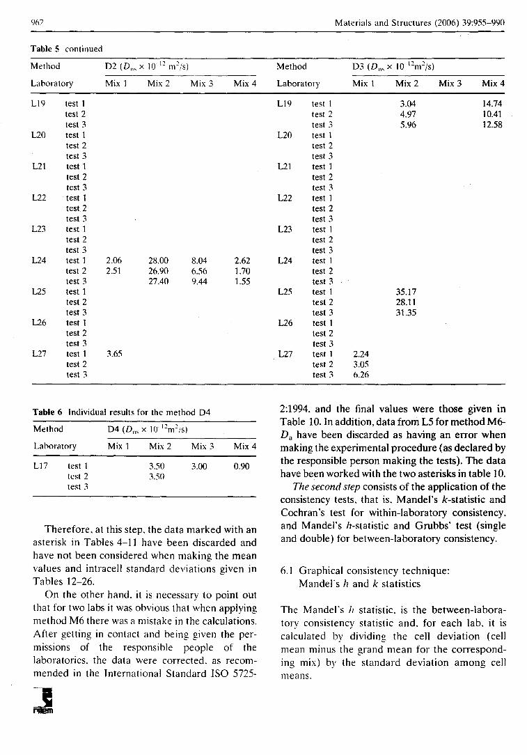
Tables 4-6 present the individual results forthe diffusion tests. It has to be noticed that only2 laboratories have performed the DI (No. 4and 12) and D1-P (No. 12 and 22) methods,probably due to the long term needed to obtainthe results and the need to take a high numberof samples. "No results" in Table 4 means thateven though the tests were prepared, there wasnot enough time to obtain any results. D2 andD3 have been performed for a higher numberof labs: 17, 15. 14 and 11 for D2 and 9, 12, 7and 4 laboratories for method D3 for mixes 1,2,

Table 3 Mixture proportions of the concretes manufactured for the RRT

kg/m'~ LabelMineral addition

Cast byCement

Silica fume

FlyashSlagWaterSand

Coarse aggregate

Total aggregateSuper-plasticisers

Air contentw/c

w/b

Strength (MPa)Slump (mm)

Mix 1Silica-fume

CHALMERS (Sweden)399

1-42.5 N V/SR/LA

21 (slurry)

]68

842.5 (0-8 mm)

842.5 (8-16 mm)

16853.4

Cementa 92M6%0.420.4063

Mix 2Plain OPC

1ETcc (Spain)400

1-42.5 R/SR

180

742 (0-6 mm)

1030 (6-]6 mm)

17724.8Melcret 222

0.45

0.45

45

> 150

Mix 3

Flyash

LNEC (Portugal)340

1V/B 32.5 R

In the cement

]53

62 (0-2 mm)603 (0-4 mm)619 (4-12 mm)555 (12-25 mm)18234.1

Rheohuild 1000

0.4552.6

Mix4

Slag

TNO (Netherlands)350IJI/B 42.5 LH HS

In the cement157.5

70 (0-1 mm)790 (0-4 mm)1040 (4-16 mm)

18303.9

Cretoplast1.5

0.45

960

Table 4 Individual results for methods DI and DI-P


Method DI(DI1, x lO-Jeme/s) MethodDI-P (DI1, x IO-'eme/s)

Laboratory

Mix 1Mix 2Mix 3Mix 4LahoratoryMix 2-curing IMix 2-curing 2

L4

test INo results1.240.600.61Ll2test 122.00 10.50test 2

No results1.771.000.46 test 2test 3

No results1.80 test 3Ll2

test 10.96 2.65 L22test 114.00 8.70test 2

No results3.87 test 216.00 9.00test 3

test 311.00 8.60

3 and 4, respectively. In the case of D4, it has

only been performed for 1 lab (lab No. 17) andnot even for every mix.

Table 7 presents the individual results for theresistivity tests. It can be noticed from this Table,that most of the laboratories have performed theR1 method (12 labs). On the opposite, only 3laboratories ha ve performed the R2 method.

In Tables 8-10, the individual values obtained

for the migration methods are given. Concerningthese methods, it can be said that in general morelaboratories have performed them, as in everycase there are enough data to perform the statistical analysis.

In Table 1L the results obtained for the con

centration of total chlorides, at the depth in whichthe colourimetric front is revealed, are given. Itcan be observed that very few labs have performed these tests.

Application of the statistical analysis is onlypossible if there are enough laboratories performing the tests. So, for methods DI, DI-P, D4,R2 and CL it was not possible to apply the statistical treatment.

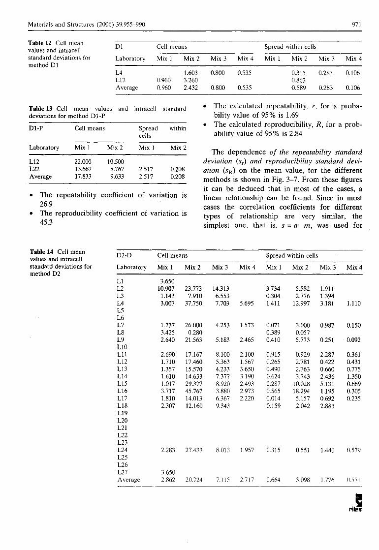
Tables 12-26 present the cell mean values andthe intracell standard deviations. derived from

Tables 4-11. for every method. calculatedaccording to procedures given in the lnternationalStandard ISO 5725-2:1994 [26].

In Table 27, a compilation of the number oflaboratories performing each method for everymix has been summarised.

6 Statistical anal~'sis of the data

The statistical treatment of the data has been

carried out according to the lnternational

Standard ISO 5725-2:1994 [26] for the determination of the accuracy (trueness and precision) oímeasurement methods and results. Part 2: Basic

method for the determination oí the repeatabilityand repraducibility oí a standard measurementmethod.

According to this standard, the parameters tobe calculated are the mean va/ue (m), therepeatability standard deviation (sr), the reproducibility standard deviation (SR), and the relationship between 111and (sr), (SR)' Inaddition, thevalues of the repeatability and reproducibi/ity, rand R, calculated for a 95% oí probability havebeen also derived.

As a first step in the statistical treatment, it isnecessary to critically examine individual values(Tables 4-11) in order to find entries that areconsidered irreconcilable with the other data.

According to the standard, when several unexplained abnormal test results occur at differentleveis within the same laboratory, then, thatlaboratory may be considered to be an outlier.It may then be reasonable to discard some orall of the data from such an outlying laboratory.In addition, the standard points out that obviously erroneous data should be corrected ordiscarded.

When the abnormal results do not occur clearlyat every leve!. in this first analysis, only obviousindividual discordant data have been taken out

because if further treated according to this standard, all the individual data fram the lab would

have been discarded: even if they are only oneindividual data they are aberrant. When all theindividual data belonging to one lab are discordant fram the rest. they have been examined inthe systematic application of statistic tests foroutliers included in the standard (step 2).

Materials and Structures (2006) 39:955-990 961

Table 5 Individual results for methods D2 and D3Method

D2 (Dos x 10-12 m2¡s) MethodD3 (Dl1s x 1O-12m2¡s)

Laboratory

Mix 1Mix 2Mix 3Mix 4LaboratoryMix 1Mix 2Mix 3Mix 4

U

test 13.65 Utest 11.5291.893.57test 2

test 21.99288*4.50test 3

test 31.6750.363.47L2

test 112.3329.6213.21 L2test 18.3225.4413.16test 2

13.7223.2016.52 test 26.3841.259.91test 3

6:6718.5013.21 test 37.0745.7513.91L3

test 11.3811.107.88 L3test 13.382.467.10test 2

0.806.595.10 test 23.922.189.62test 3

1.256.046.68 test 34.652.4814.90LA

test 14.6352.354.884.91LAtest 11.1732.297.882.23test 2

2.3133.467.086.48 test 21.7434.218.143.52test 3

2.0827.4411.1515.19* test 31.9350.275.12L5

test 1 L5test 11.7317.532.832.51test 2

test 21.6617.024.082.62test 3

test 3L6

test 1 L6test 1test 2

test 2test 3

test 3L7

test 11.6626.003.121.65L7test 1test 2

1.8029.004.921.67 test 2test 3

1.7523.004.721.40 test 3LB

test 13.150.24 LBtest 15.141.67test 2

3.700.32 test 24.391.55test 3

test 3L9

test 12.9315.235.462.40L9test 1test 2

2.3522.935.122.53 test 2test 3

26.534.97 test 3UO

test 1 UOtest 1 13.07test 2

test 215.63test 3

test 3U1

test 12.0116.909.001.80U1test 1test 2

3.7318.205.502.50 test 2test 3

2.3316.409.802.00 test 3U2

test 12.0117.945.111.90U2test 11.8227.808.362.10test 2

1.6119.975.851.08 test 21.8332.509.422.85test 3

1.5114.475.131.72 test 31.7034.529.412.20LB

test 11.0315.014.424.43LBtest 1test 2

1.1213.134.782.88 test 2test 3

1.9218.573.503.64 test 3U4

test 11.2411.907.461.91U4test 1test 2

2.3313.104.903.06 test 2test 3

1.2618.909.774.60 test 3U5

test 10.6918.196.162.03U5test 10.9824.292.26test 2

1.2332.385.762.19 test 21.4625.103.71test 3

1.1337.5614.843.26 test 32.0328.534.68U6

test 14.3242.705.172.97U6test 1 6.52test 2

3.2065.402.813.28 test 216.72test 3

3.6329.203.662.67 test 3L17

test 11.8212.705.842.11L17test 1test 2

1.8019.706.112.06 test 2test 3

9.647.152.49 test 3L18

test 12.3510.0312.49 L18test 1test 2

2.1312.358.71 test 2test 3

2.4414.106.83 test 3

962 Materials and Structures (2006) 39:955-990

Table 5 continuedMethod

02 (Dns x 10 1" m"/s) Method03 (Dns x 10 ("m"/s)

Lahoratory

Mix 1Mix 2Mix 3Mix4LaboratoryMix 1Mix 2Mix3Mix4

L19

test 1 L19test 1 3.0414.74test 2

test 24.9710.41test 3

test 35.9612.58L20


test 2test 3

test 3L21


test 2test 3

test 3L22

test 1 L22test 1test2

test 2test 3

test 3L23


test 2test 3

test 3L24

test 12.0628.008.042.62L24test 1test 2

2.5126.906.561.70 test 2test 3

27.409.441.55 test 3L25

test 1 L25test 1 35.17test 2

test 228.11test 3

test 331.35L26


test 2test 3

test 3L27

test 13.65 L27test 12.24test 2

test 23.05test 3

test 36.26

Table 6 Individual results for the method 04

J

Therefore. at this step, the data marked with anasterisk in Tables 4-11 have been discarded and

have not been considered when making the meanvalues and intracell standard deviations given inTables 12-26.

On the other hand. it is necessary to point outthat for two labs it was obvious that when applyingmethod M6 there was a mistake in the calculations.

After getting in contact and being given the permissions of the responsible people of thelaboratories. the data were corrected. as recommended in the lnternational Standard ISO 5725-

The Mandel's h statistic. is the between-Iabora

tory consistency statistic and. for each lab, it iscalculated by dividing the cel1 deviation (cel1mean minus the grand mean for the corresponding mix) bv the standard deviation among cell~ . ~means.

6.1 Graphical consistency technique:Mandel's h and k statistics

2:1994. and the final values were those given inTable 10. In addition, data from L5 for method M6Da have been discarded as having an error whenmaking the experimental procedure (as declared bythe responsible person making the tests). The datahave been worked with the two asterisks in table 10.

The second step consists of the application of theconsistency tests. that is, Mandel's k-statistic andCochran's test for within-Iaboratory consistency.and Mandel's h-statistic and Grubbs' test (singleand double) for between-Iaboratory consistency.

Mix 4

0.90

Mix 3

3.00

Mix 2

3.503.S0

Mix 1

test 1test 2test 3

Lahoratory

L17

Method


Table 7 Individual results for methods R 1 and R2 Method

R1 (ohm cm) MethodR2 (ohm cm)

Laboratory

Mix 1Mix2Mix 3Mix4LaboratoryMix 1Mix 2Mix 3Mix4

L1


test 2test 3

test 3L2


test 2test 3

test 3L3


test 2test 3

test 3L4

test 11557254502041020734L4test 1test 2

1556764002042421164 test 2test 3

1760356601994916270 test 3L5

test 12969658502397634349L5test 1test 2

3045252171921036592 test 2test 3

test 3L6


test 2test 3

test 3L7

test 131920109692128446753L7test 1test 2

3348693282194946645 test 2test 3

3050894333214342976 test 3LB

test 1305283676 LBtest 1test 2

297655727 test 2test 3

test 3L9


test 2test 3

test 3LlO

test 1 6405 LlOtest 1test 2

6316 test 2test 3

test 3L11

test 13668067591930046800L11test 133000600019900test 2

3638365212210039800 test 235100610022700test 3

3283067872290041300 test 331800640023500Ll2

test 12512258142291034242L12test 1test 2

2678951761763038877 test 2test 3

2617458831924736691 test 3L13

test 1183005970155400*28100L13test 1test 2

155009020158700*29900 test 2test 3

237009960158700*8800* test 3Ll4

test 14485117849*2871347015L14test 1test 2

4060417058*2907448694 test 2test 3

4259721237*2962945245 test 3Ll5

test 14066356513712040293L15test 1test 2

3920352864364839550 test 2test 3

3430349463867334048 test 3Ll6


test 2test 3

test 3Ll7

test 13470175702516931817L17test 1test 2

3091976052603830650 test 2test 3

2564775632290536257 test 3Ll8

test 141850870030680 L1Stest 1test 2

42100835028090 test 2test 3

37760841027560 test 3L19

test1 L19testl



Rl (ohm cm) MethodR2 (ohm cm)

Laboratory

Mix 1Mi" 2Mix 3Mix 4LahoratoryMix 1Mix2Mix 3Mix 4

test 2

test 2test 3

test 3L20


test 2test 3

test 3L21


test 2test 3

test 3L22

test 1 L22test Itest 2

test 2test 3

test 3L23

test 1 L23test Itest 2

test 2test 3

test 3L24

test 1 L24test 132300106193033950781test 2

test 225050110892927948494test 3

test 336310138763171249119L25


test 2test 3

test 3L26

test 1 96002340039100L26test 1test 2

120002606637900 test 2test 3

1110024900 test 3L27


36400 test 238300test 3

32700 test 332100

The Mandel's k statistic, is the within-labora

tory consistency statistic and, for each lab, it iscaIculated by dividing the intracell standard

deviation by the pooled within-cell standarddeviation for each mix.

The h and k values are plotted for each cell inorder of laboratory, in groups for each mix (and

separately grouped for the several mixes examined by each laboratary). Examination of these

plots may indica te that specific laboratories exhibit patterns of results that are marked different

fram the others in the study.

The numerical technique has been applied inthe following way:

• If the test statistic is less than or equal to its

5% critical value, the item tested is acceptedas correct.

• lf the test statistic is greater than its 5 %

critical value and less or equal to its 1%critical value, the item tested is called a

straggler. and is marked as it. but it is retained as correct.

• If the test statistic is greater than its 1% critical value, the item tested is called outlier, it is

marked as it and in general, it is discarded.

The details of these tests are properly de

scribed in the Standard ISO 5725. An example ofthe application of this test to D2 method is givenin Figs. 1 and 2, where Mandel's h and k statistic

are plotted, respectively. According to these figures, concerning Mandel's h statistic, laboratory 2is an outlier for mixes 1 and 3: lab 4 is an outlier

far mix 4 and lab 16 is and straggler for mix 2.Concerning Mandel's k statistic (Fig. 2), labs 2, 15

and 16 are outliers for mix 1, 3 and 2, respectively.Labs 4 and ]4 are stragglers far mixes 2 and 4,

respectively.

In these pictures, the depicted critical values

have been those corresponding ~o the maximumnumber of participating labs; however, when

making the calculations, the specific number oflabs in each level (for each mix) have beenconsidered. The results obtained fram these

techniques. with detailed indication of straggler


Table 8 Individual results for the methods MI and M3Method

MI (Charge passed, C) MethodM3 (Dns x 1O-12m2/s)

Laboratory

Mix 1Mix 2Mix 3Mix4LaboratoryMix 1Mix2Mix 3Mix4

U

test 1 Utest 1test 2

test 2test 3

test 3L2


test 2test 3

test 3L3


test 2test 3

test 3L4

test 19303248859623L4test 1test 2

9523558759699 test 2test 3

4762832665 test 3L5

test 16552028688574L5test 10.430.730.660.50test 2

6463344761555 test 20.350.951.050.50test 3

test 3L6


test 2test 3

test 3L7

test 17053118897565L7test 10.301.200.600.30test 2

7143535812538 test 20.301.000.500.30test 3

7623132957516 test 30.401.000.600.30L8


7112620 test 2test 3

test 3L9

test 1 2413905416L9test 1test 2

2979898454 test 2test 3

29001071 test 3UO

test 1 UOtest 1test 2

test 2test 3

test 3U1

test 1 U1test 10.620.79test 2

test 20.611.1test 3

test 30.810.88U2

test 17352700850554U2test 11.561.9281.631.55test 2

6193106957585 test 21.581.5241.541.68test 3

34338651914* test 31.641.5531.711.64LB

test 1 3701878396LBtest 10.0930.20.240.08test 2

2531850439 test 20.1360.250.160.06test 3

23778192180* test 30.230.130.1U4

test 1 U4test 123.1 *64.31*33.63*0.497test 2

test 282.45*63.68*49.83*0.406test 3

test 399.76*63.38*65.02*0.39U5

test 14513453532464U5test 115.21.50.7test 2

5453250551513 test 20.85.81.50.4test 3

4364242495524 test 30.84.72.10.9U6

test 1 U6test 11.37 6.332.8test 2

test 21.53 5.993.02test 3

test 31.1 2.92U7

test 1 U7test 10.310.610.30.2test 2

test 20.380.50.350.25test 3

test 30.330.630.340.29U8

test 1 U8test 11.412.391.31test 2

test 21.62.831.94test 3

test 32.262.140.97



MI (Charge passed, C) MethodM3 (Dns x 10 121112/S)

Laboratory

Mix 1Mix 2Mix 3Mix4LaboratoryMix 1Mix 2Mix3Mix4

L19


test 2test 3

test 3UO

test 1 1474 UOtest 1test 2

1956 test 2test 3

1935 test 3L21

test 1 3558 L21test 1test 2

3736 test 2test 3

3647 test 3L22

test 1 U2test 1test 2

test 2test 3

test 3L23

test 18203378371734L23test 1test 2

7622480493733 test 2test 3

7382524514653 test 3L24

test 16402996655436L24test 1test 2

6322420662476 test 2test 3

7682391676441 test 3L25


test 2test 3

test 3L26

test 1 2661720404L26test 1test 2

1896591502 test 2test 3

2219648467 test 3L27


test 2test 3

test 3

and outliers are given in Tables 28Natural diffusion/Resitivity andrespectively.

6.2 Cochran's test

and 29 for

Migration.values according to Cochran's test have alsobeen specified.

6.3 Grubbs's test

The Standard ISO 5725 assumes that between

laboratories only small differences exist in therepeatability variances. However. this is notalways the case, so Cochran 's test has been recommended to check the validity of this assumption. The details of this test are properlydescribed in the Standard ISO 5725. but in

summary. a parameter. Cochran's test statistic,C. is calculated and compared with its 1% and5% critical values with the same criterion as tha!in the case of Mandel's stalistics. In Tables 28

and 29 for Natural diffusion/Resitivity andMigration, respectively, straggler and outlier

The aim of this test is the same as that of Coch

ran 's test but regards the reproducibility variancesby testing the significance of the largest observation (sh). of the smallest observation (sI), of thetwo largest observations (dh) and the two smallestobservations (dI). The details of these tests areproperly described in the Standard ISO 5725. butin summary, for these four cases the Grubb'sstatistics are computed and they are comparedwith the critical values for Grubbs's test. In Ta

bles 28 and 29 for Natural diffusion/Resitivity andMigration. respectively. straggler and outlier values according to Grubbs's test have also beenspecified.


Table 9 Individual results for methods M4 and M5.Method

M4 (D"s x 10 Jcmc/s) MethodM5 (D"s x 10 Jcmc/s)

Laboratory


L1

test 1 Utest 1test 2

test 2test 3

test 3L2


test 2test 3

test 3L3

test 12.109.803.10 L3test 1test 2

2.709.903.90 test 2test 3

2.9012.204.40 test 3L4

test 16.4015.803.701.80L4test 10.8422.104.236.50test 2

5.0017.005.203.30 test 22.1516.704.513.70test 3

2.3014.00 4.10test 33.0613.004.032.08L5

test 1 L5test 11.4615.304.010.99test 2

test 21.4513.406.751.11test 3

test 3L6

test 10.777.760.98 L6test 1test 2

7.231.41 test 2test 3

5.16 test 3L7

test 11.6012.903.701.70L7test 1test 2

2.1015.1O5.301.60 test 2test 3

1.5014.504.501.60 test 3L8

test 10.301.30 L8test 10.150.322*test 2

0.100.60 test 20.120.2*test 3

test 3L9

test 13.4011.507.102.90L9test 1test 2

3.0011.005.602.80 test 2test 3

8.907.30 test 3UO


test 2test 3

test 3L11

test 12.6016.307.302.40Ultest 1test 2

2.7015.907.303.20 test 2test 3

3.0014.108.602.40 test 3L12

test 12.2015.508.301.80U2test 12.0417.93.631.13test 2

2.7017.006.702.34 test 21.315.64.361.53test 3

3.4015.607.501.68 test 31.2728.6 1.13U3

test 12.7015.103.802.30U3test 1test 2

2.0017.006.002.80 test 2test 3

2.7015.304.603.60 test 3U4

test 11.8012.804.302.50L14test 1test 2

1.9018.603.502.00 test 2test 3

2.0014.103.302.10 test 3L15

test 12.8017.703.202.20L15test 11.1343.22.330.56test 2

4.3017.203.202.50 test 21.2653.44.660.402test 3

3.4015.706.002.30 test 31.5394.31.131.2L1ó

test 11.594.40 2.40Ll6test 1test 2

2.904.70 S.11;.test 2test 3

2.003.10 3.60test 3L17

test 13.1014.904.802.20Ll7test 1test 2

3.0014.805.702.90 test 2test 3

3.0014.905.402.90 test 3LIS

test 12.0015.403.40 L1Stest 1test 2

2.6021.206.50 test 2test 3

2.3013.604.00 test 3

96S Materials and Structures (2006) 39:955-990


M4 (D,,, x lO-l"m"/s) MethodM5 (D,,, x ]0 121112/S)

Laboratory


L19

test 1 8.500.30L19test 1test 2

9.201.00test 2test 3

9.200.90test 3L20


test 2test 3

test 3L21


test 2test 3

test 3L22


test 2test 3

test 3L23


test 2test 3

test 3L24

test 12.7017.60R.202.90L24test 1test 2

5.3015.606.503.60 test 2test 3

2.2012.308.302.60 test 3L25


test 2test 3

test 3L26

test 1 13.717.803.34L26test 1test 2

12.965.003.34 test 2test 3

12.815.403.18 test 3L27

test 11.70 L27test 1test 2

1.90 test 2test 3

2.70 test .3

6.4 Criteria for rejection of data

The criteria followed to reject data have been thefollowing: to reject one set of data, it should beclassified as outlier by both within-Iaboratoryconsistency statistic (Mandel's k-statistic andCochran's tests) or by both between-Iaboratoryconsistency statistic (Mandel's h-statistic andGrubb's tests) or by one of the within-Iaboratoryand one of the between-Iaboratory consistencystatistic tests.

6.5 Calculation of the statistical data

For the calculation of the values of the repeatability standard deviation, Sr' and reproducibilitystandard deviation. SR, it is necessary to calculatepreviously the variance of repeatability (s;) andthe variance of reproducibility (sD. according tothe equations detailed in the Standard ISO 5725.From them, it is possible to calculate the values of

repeatability and reproducibility for a givenprobability. In the case of a 95% probability:

r = 2.83[ii and R = 2.83Vs[ + s~

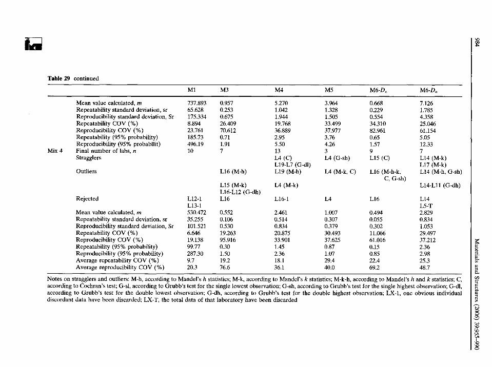
The statistical values determined according tothe standard ISO 5725, as well as the details on

the stragglers and outliers according to the different methods applied and then the laboratoriesdiscarded and retained for the study are presented in Tables 28 and 29 for Natural diffusion/

Resitivity and Migration, respectively.For a better understanding of Tables 28 and 29,

a detailed example of the meaning of the symbolsand abbreviations used (for method D2 and mix1) is as follows:

• The I1I1l11berof laborlllOries, 11, that finally hasbeen included for the calculations of the

repeatability and reproducibility coefficientsof variation is 16

Materials and Structures (2006) 39:955-990 9<íY

Table 10 Individual results far the methad M6 (Steady state coefficient, De, and non steady state coefficient DJMethod

M6-Dc' (DIl, x 10 121112/S) Method12 2

M6-D" (Dn, x 10m /s)

Laboratory


L1


test 2test 3

test 3L2


test 2test 3

test 3L3


test 2test 3

test 3L4

test 10.601.100.300.30L4test 15.235.191.893.85test 2

1.102.100.100.30 test 25.505.162.762.98test 3

0.401.00 test 32.674.70L5

test 10.591.950.520.50L5test 10.76**1.35**0.56**0.52**test 2

0.351.680.480.50 test 20.67**1.58**0.92**0.52**test 3

test 3L6


test 2test 3

test 3L7

test 11.203.202.000.90L7test 12.9524.187.443.01test 2

1.502.801.600.90 test 22.569.065.973.21test 3

1.602.501.800.80 test 36.7814.735.913.49L8

test 11.501.70 L8test 14.538.99test 2

1.70 test 24.53test 3

test 3L9


test 2test 3

test 3UO


test 2test 3

test 3Ul

test 10.421.430.370.19Ultest 14.816.417.63.9test 2

0.281.730.290.22 test 24.515.145*3.8test 3

0.461.470.360.19 test 37.617.410.54.1U2

test 11.332.11.0550.59U2test 14.213.69.272.28test 2

1.882.10.620.66 test 24.89188.482.57test 3

2.19 1.650.67 test 34.67 3.7LB

test 1 0.720.08LBtest 1 27 1.55test 2

0.150.87 0.09test 24.4618.68 1.54test 3

0.280.930.540.156 test 35.418.826.791.54U4

test 10.421.270.310.54U4test 110.223.0127.258.98test 2

009*1.570.40.495 test 29.123.6616.6911.5test 3

0.1111.590.350.605 test 310.422.0217.3U5

test 13.55.32.71L15test 1n.996.332.192.8test 2

2.75.72.90.8 test 21.565.792.772.44test 3

5.62.21 test 3 6.482.923.39U6

test 1 0.133.04L16test 1test 2

3.05*4.49 test 2test 3

0.173.84 test 3L17

test 10.91.50.420.3L17test 15.5222.99.692.5test 2

0.91.10.58n.3 test 27.622.910.63.8test 3

0.61.20.590.27 test 36.1524.29.230.13L18

test 10.8940.4 L18test 154 49test 2

0.923.810.8 test 2141test 3

50*2.620.86 test 36584L19

test I L19test 1

.~

pilem

970

Table 10 continued


Method M6-Dc' (D", x lO-lcmc/s) MethodM6-D" (D"s x 1O-lcmC/s)

Laboratory

Mix]Mix 2Mix 3Mix4LaboratoryMix ]Mix 2Mix3Mix4

test 2

test 2test 3

test 3L20

test] L20test ]test 2

test 2test 3

test 3L2]

test 1 L2]test ]test 2

test 2test 3

test 3L22

test I L22test 1test 2

test 2test 3

test 3L23

test ] L23test 1test 2

test 2test 3

test 3L24

test ] L24test]test 2

test 2test 3

test 3L25


test 2test 3

test 3L26


test 2test 3

test 3L27

test I L27test 1test 2

test 2test 3

test 3

Table 11 Individual resusts for the Colourimetric method C] using AgNo., and AgNo.'1 and K::Cr04

Method

C](% Cn with AgNo.'1 MethodC1(% Cn with AgNo.'1 and K::Cr04

Laboratory

Mix ]Mix 2Mix 3Mix 4LahoratoryMix 1Mix 2Mix 3Mix4

L5

test I0.0620.1340,()490.100L5test 10.0490.1370.0520.]00test 2

0.0270.1680.0990.100 test 20.0190.]790.1190.100test 3

test 3L8

test I0.849 L8test 10.849test 2

test 2test 3

test 3L12

test 10.055O.]] O0.2500.125L12test 10.0520.1500.290test 2

0.0280.]200.3200.06] test 20.0400.0600.270test 3

test 3

• Laboratory No. 11 (L11) is an straggleraccording to the Cochran 's test

• The laboratory No. 2 (L2) is an outlieraccording to Mandel's h and k statistic,

Cochran's test and according to Grubb's test

for the single highest observation.• Laboratory 4 (L4) is an outlier according to

Cochran's test

eli'iiIem

• Therefore, Laboratory 2 (L2) has been

rejected for further analysis• The mean value, 111, for the 16 remammg

laboratories is: 2.212

• The repeatability standard deviation, SI"' is0.596

• The reproducibility standard deviation, SR, is1.003

Materials and Structures (2006) 39:955-990 97]

Table 12 Cell mean

D]Cell means Spread within cellsvalues and intracell

standard deviations forLaboratoryMix]Mix2Mix 3Mix 4Mix 1Mix2Mix 3Mix 4

method DI L41.6030.8000.535 0.3150.2830.106

L120.9603.260 0.863

Average

0.9602.4320.8000.535 0.5890.2830.106

Table 13 Cell meanvaluesandintracellstandarddeviations for method DI-P

D1-P

Cell meansSpreadwithincells --Laboratory

Mix 1Mix 2Mix 1Mix 2

L12

22.00010.500L22

13.6678.7672.5170.208

Average

17.8339.6332.5170.208

• The repeatability coefficient of variation is26.9

• The reproducibility coefficient of variation is45.3

• The calculated repeatability, r, for a probability value of 95% is 1.69

• The calculated reproducibility, R, for a probability value of 95% is 2.84

The dependence ol the repeatability standarddeviation (sr) and reproducibility standard deviation (SR) on the mean value, for the differentmethods is shown in Fig. 3-7. From these figuresit can be deduced that in most of the cases, alinear relationship can be found. Since in mostcases the correlation coefficients for different

types of relationship are very similar, thesimplest one, that is, s = a' m, was used for

describing the dependency. In such a relationship, the slope a describes the mean coefficientof variation (COY). It is worth to remark thatwith the mean values of the data in this research,

in which three values are considerably smaller

than the fourth one, the slope of the regression ismuch conditioned by the highest data. Therefore,even though these values have been calculated

(and given in Figs. 3-7) with the correlation

eoeffieients, the mean COY value that is going to

be eonsidered in the subsequent treatment is

ealculated from the average of those eorre

sponding to every mix whieh is given inTables 28 and 29.

7 Discussion

7.1 Methodology for evaluation

In order to make a more comprehensive evalu

ation, rather than only a consideration of theprecision of the methods, four indicators relatedto both the obtained results and the character

istics of the methods have been identified to be

taken into account: (1) The trueness, (2) The

precision, (3) The relevance and (4) The convemenee.

They will be explained in more detail whenapplying to the differenl methods.

974 Materialsand Structures(2006)39:955-990

Table 19 Cellmea n

MICellmeans Spread withincellsvaluesand intracell

standarddeviationsforLaboratoryMix 1Mix 2Mix 3Mix 4Mix 1Mix2Mix3Mix4

method MI UL2L3L4

78632137616612693649754

L5

651268672456569315113

L6 L7

7273262889540312377325

L8

7232870 16354

L9

2764958435 3079827

UO UlU2

6773080891570823675822

U3

2870849418 7243030

U4 U5

4773648526500595242832

U6 U7U8U9L20

1788 272

L21

3647 89

L22 L23

7732794459707425067746

L24

6802602664451763411122

L25 L26

2259653458 3846550

L27 Average

6872883737530734155932

In order to make the scoring of the methods,each of these sub-indicators has been classified in

three categories, divided according to an incremental favourable significance.

The indicators, sub-indicators and an exampleof limits for the scoring are given in Table 30.For each sub-indicator, the worst category hasbeen assigned 1 point, 2 for the medium one and3 points for the better characteristics of themethod. Therefore, for the first sub-indicator,there is a total score of 3 points, as the two subindicators exclude mutually, 6 for the secondone, 6 for the third one and 12 for the fourthone.

Then, it is necessary to take the average of theweight of each indicator. As a first step, the sumof the points of the different sub-indicators corresponding to each indicator is divided by thetotal points available for that indicator: that givesthe scorelindicator. For example a method having6 points for a total of 6 on a indicator will have"1" for that indicator.

Then, the score/indicator is multiplied by afactor of importance, F.l., that depends on theweight that the indicator is considered to have. Ifa11the indicators have the same weight, the El. is1 for a11of them.

7.2 Application of the proposed methodology

7.2.1 Trueness

The term "trueness" describes the closeness of

agreement between the arithmetic mean of anumber of test results and the true or acceptedreference value.

The mean values obtained, for the differentmixes, are given in Figs. 8 and 9 for steady stateand non-steady state coefficients, respectively.The error bars indicate, in percentage on themean, the averaged standard deviation of reproducibility for the corresponding method.

The methods having an asterisk in the legend01' the figures are those for which the statistical


Table 20 Cell mean

M3Cell means Spread within cellsvalues and intracell

standard deviations forLahoratoryMix 1Mix 2Mix 3Mix 4Mix 1Mix 2Mix 3Mix 4

method M3 UL2L3L4L50.3900.8400.8550.5000.0570.1560.2760.000

L6 L70.3331.0670.5670.3000.0580.1150.0580.000

L8 L9UOU10.6800.923 0.1130.159

U21.5931.6681.6271.6230.0420.2250.0850.067

LB0.1150.2270.1770.0800.Q300.0250.0570.020

U40.4310.058

U50.8675.2331.7000.6670.1150.5510.3460.252

U61.3336.1602.9130.217 0.2400.110

U70.3400.5800.3300.2470.0360.0700.0260.045

U81.7572.4531.407 0.4460.3490.492

U9 L20L21L22L23L24L25L26L27Average

0.8231.6241.6030.8450.1240.2060.1980.069

treatment could not be applied due to the smallnumber of data.

Concerning the steady state, the method considered as a reference to be used as a target valueis method DI, which is the natural diffusion one.However, it has to be pointed out that the valuesobtained trough this method are not statisticallysignificant, as for most of the mixes, only onevalue is available. Therefore, both sub-indicators,1-1 and 1-2 will be calculated in order to obtain a

better estimation of the bias with respect to thetarget value. In the case of non-steady-state tests,it is known that different experimental conditionscan lead to different results. However. as it can be

seen in Fig. 9, the results obtained using botbmethods D2 and D3, in natural diffusion conditions, lead to very similar results. Therefore, the"true value " to be considered in tbis case has

been the mean value of the results given by bothmethods.

The averaged percentages of bias with respect to the mean value for the differentmethods are given in Table 31. From the results in Table 31 it can be deduced that for

the steady state coefficients using both criteria(DI and the average as target values) theresulting score is the same. The comparisonbetween the methods indicates tbat using bothcriteria, M6-Ds is the metbod having theslowest bias and M3 is the method having thehighest one.

Concerning non-steady state coefficients, D4has almost a 70% bias from the target valuecorresponding to the average of D2 and D3. Therest of the migration methods have 2 points asscore and M4 has lesser bias (20%) while M5 hasbigher bias (43 %). On the other hand, it isremarkable tbat all the methods, with the exception of M6-Dns, give smaller values than tbat al'tbe target value.

976 Matcrials and Structures (2006) 39:955-990

Table 21 Cclll1lcanva1ues and intraccllstandard deviations [ormethod M4

M4

Laboratory

Cell I1ll'anS

Mix 1 Mix 2 Mix 3 Mix 4

Spread within cells

Mix \ Mix 2 Mix 3 Mix 4

2.567 lOA'",3.800 0.4161.3580.6564.5(,7

15.(,004.4503.0(¡72.0l-:41.5101.0611.1(,X

0.77\

6.7141.197 1.3750.3011.733

14.1674.500\.6330.32\1.1370.800O.05X0.200

0.950 0.1410.4953.200

10.4676.6672.8500.2831.3800.9290.071

2.767

15.4137.7332.6670.2081.1720.7510.4622.767

16.0337.500\.9400.6030.8390.8000.3522.467

15.8004.8002.9000.4041.0441.1140.6561.900

15.1673.7002.2000.1003.0440.5290.2653.500

16.8674.1332.3330.7551.0411.6170.1532.1C,3

4.067 3.000O.ri700.850 0.8493.033

14.8675.3002.11670.0580.0580.4580.4042.300

\6.7334.ri33 0.3003.9721.6448.967

0.7330.4040.379

LIL21.3lAL51.6L7LHL9LlO

LllLl2Ll3Ll4Ll5LI6Ll7Ll8Ll9L20L21L22L23L24L25L26L27

Average

3.400

2.1002.465

\5.167 7.ri67

13.160 6.067

12.399 5.153

3.033

3.2X5

2.485

l.ri(i4

0.5290.569

2.67ri

0.482

1.343

1.012

\.514

0.942

0.513

0.095

0.417

7.2.2 Precisioll

The term "precision" refers to the c10seness ofagreement between the results,

Providing that the number of labs performingthe methods DI, Ol/P, 04, R2 and el are notstatistical1y representative, even though the values reported by the different labs are given in thecorresponding tables, it was not possible to gofurther in the analysis. Therefore, provided themethodology proposed here, they won't be t~eninto account in the further scoring.

The averaged coefficients of reproducibility andrepeatability for the rest of the methods are givenin Tables 28 and 29. For the sake of c1arity, themean values are also depicted in Fig. 10.

From Fig. 10 it can be deduced than in general,the accuracy of these methods is not very gooó.'mainly as long as reproducibility conditions areconcerned.

As expected, the values for repeatability, sr/m

(%), are much lower than .\'R/m (%), being the

highest ones M5 and 02, that reach almost a30%. The lowest ones are the measurement of

the resistivity (R 1) and the standard ASTM C1202-97 (MI), with values smaller than a 10%.

For the coefficient of variation for reproducibility values, the highest values can be foundwhen caIculating the steady state diffusion coefficients in migration cel1s (M3 and M6-De) beingthe highest one that of M3. The lowest ones areagain that of (R 1) and (MI).

The values and the corresponding score to thesub-indicators selected and given in Table 30, aregiven in Table 32.

7.2.3 Relevance

This indicator "relevance" refers to the quality ofthe information that each method provides.Concerning this point, the first sub-indicator (3-1)refers to the diffusion coefficients Ds and Dos.

On one hand, the standard ASTM C-1202-97,covers the determination of the electrical


Table 22 Ccll mcan

M5Ccll Illcal1S Sprcall wilhin ccllsvalucs anll inlraccll ------.---------.------------.------

slanllarllllcvialiolls rol' LahoratoryMix 1Mix 2Mix 3Mix 4Mix 1Mix 2Mix 3Mix4mClholl M5 LIL2L3

...,

L42.01817.2674.2574.0931.1144.5760.2412.236

L51.45514.3505.3801.0500.0071.3441.9370.085

L6 L7U\O.DI 0.023

L9 LlOL11

...

L121.53720.7003.9951.2630.4366.9380.5160.231

L13 L14L151.30763.6332.7070.7210.20427.0431.7950.423

Ll6 L17L18L19L20Ir

L21L22L23.L24L25L26L27Avcragc

1.2H92H.9HH4.0H5I.7H2O.:l579.9751.1220.744

conduclance of concrete to provide a rapid indication of its resislance lo lhe penelralion 01"

chloride ions, nol giving any parameter ahle lo heused to make predictions. The calculalion of lheresistivily (method R 1), withoul any additionalcalculation, do not provide any of lhe coefficienls.Therefore, they are given 1 point.

On the olher hand there are several melhods

that provide a single diffusion coefficient. Theyare: 02, 03, RI/M, M3, M4 and M5. 02, 03, M4and M5 give the value of the non-steady state andRlIM and M3 give the steady state diffusioncoefficient. Therefore, they are given 2 points.

The M6 method provides simultaneously theDe and Da coefficients and the ratio between

them addresses lhe hinding ahilily 01" the matrix.necessary I"or using lhese parameters in servicelife predictions. Therefore, this method has 3

points for sub-indicator 3-1.Wilh respect to the sub-indicator 3-2: 02, even

though is a natural diffusion tesl, accelerates hy

efrect of lhe concenlration of the solution (165 gNaCI/I); lhus, il is given 2 poinls. The rest of thenatural diffusion test and resistivity melhods aregiven 3 points. MI accclerales greally by efrecl ofe1eclricallield (12 V/cm) and lherefore it is given 1poinl; the rest of migration tesl are given 2 points.

7.2.4 COl/vel/iel/ce

This indicator refers to the appropriatenessconcerning cost in hours-man and resources. Atthis respect, the assignation of methods according to the sub-indicators has be en made asfoJlows:

Suh-indicator 4-1: Handling after the test: Neednf miJling, grinding or cutting, splitting.

The most expensive melhods are those thatneed milling of the concrete specimens as theyneed a lot of hours-man. The methods that need

this kind of techniques and therefore they havelhe score 01" l poinl are the 02 and 03.


Table 23 Cell mean

M6-DeCell means Spread within cellsvalues and intracell

standard deviations forLaboratoryMix 1Mix2Mix3Mix4Mix 1Mix2Mix 3Mix4

method M6 for the ca1culation of the steady-

Llstate coefficient, De

L2L3L4

0.7001.4000.2000.3000.3610.6080.1410.000L5

0.4701.8150.5000.5000.1700.1910.0280.000L6 L7

1.4332.8331.8000.8670.2080.3510.2000.058L8

1.6001.700 0.141L9 LlOLl1

0.3871.5430.3400.2000.0950.1630.0440.017Ll2

1.8002.1001.1080.6400.4360.0000.5170.044LB

0.2150.8400.5400.1090.0920.108 0.041Ll4

0.2661.4770.3530.5470.2180.1790.0450.055Ll5

3.1005.5332.6000.9330.5660.2080.3610.115Ll6

0.1503.790 0.0280.726Ll7

0.8001.2670.5300.2900.1730.2080.0950.017Ll8

0.9053.4770.687 0.0210.7480.250Ll9 L20L21L22L23L24L25L26L27Average

1.0612.1800.8010.8180.2250.2760.1710.107

The methods M4 and MS needs immediate

splitting of the solid sample into two halves:Therefore, they areassigned 2 points.

The rest of methods: Rl/M, M1, M3 and M6are given 3 points.

Sub-indicator 4-2: Need of chloride analysis.After milling the samples in methods D2 and

D3, it is necessary to analyse the solid samples,which is quite expensive. Therefore, they have 1point as long as this sub-indicator is concerned.

M3 needs analysis of liquid samples and the M4and MS methods apply a colourimetric techniqueof analysis. Therefore, they are assigned 2 points.

The rest of methods: Rl/M, M1 and M6 do nothave analysis, so, they are given 3 points.

Sub-indicator 4-3: Difficulty of handling.The M3 and M6 method involve mounting and

preparing a migration cell and also some chemicalhandling. So, they are given 1 point. The methodsM1, M4 and MS involve montage of the cell butnot chemical handling. So, 2 points for 4-3 subindicator.

D2, D3 and Rl/M are the most easy to handle;therefore, they have 3 points.

Sub-indicator 4-4: Time consumption.D2 and D3 are natural diffusion methods, and

therefore time consuming. So, 1 point in this subindicator. The M3, M4, MS and M6 methods aremigration methods that involve from more than1 day to about 10-12 days. Therefore, they aregiven 2 points.

The M1last for 6 h and Rl/M method is almost

instantaneous. Therefore, they are given 3 points.

7.2.5 Final application

As a summary, the c1assification of the differentmethods according to these four different indicators is given in Table 33, where the points assigned to each sub-indicator for each method aregiven. In addition, the sum of the points forindicator has been made, and the score/indicator(max. 1 for each indicator) has be en calculated.The partial ranking, according to each of these


Cell meansTable 24 Cell meanvalues and intracellstandard deviations formethod M6 for thecalculation of the non

steady-state coefficient,Da

M6-Da

Laboratory

LlL2L3L4L5L6L7L8L9LlOLl1Ll2Ll3Ll4Ll5Ll6Ll7Ll8Ll9L20L21L22L23L24L25L26L27

Average

Mix 1

4.467

4.0974.530

5.6334.5874.9309.9001.275

6.42354.000

9.984

Mix2

5.017

15.9908.990

16.30015.80021.50022.897

6.200

23.33385.000

22.103

Mix3

2.325

6.440

14.0508.8756.790

20.4132.627

9.84084.000

17.262

Mix4

3.415

3.237

3.9332.8501.543

10.2402.877

2.143

3.780

Spread within cells

Mix 1 Mix 2

1.562 0.275

2.332 7.6380.000

1.710 1.1530.352 3.1110.665 4.7640.700 0.8260.403 0.363

1.067 0.75149.153

0.977 7.559

Mix3

0.615

0.867

5.0200.559

5.9290.386

0.697

2.010

Mix4

0.615

0.241

0.1530.7500.0061.7820.480

1.861

0.736

Table 25 Cell mean values and intracell standard deviations for method C1 using AgN03

Spread within cellsC1 with AgN03

Laboratory

L5LB

Ll2

Average

Cell means

Mix 1

0.0450.8490.0420.312

Mix 2

0.151

0.1150.133

Mix3

0.074

0.2850.180

Mix4

0.100

0.0930.097

Mix 1

0.025

0.0190.022

Mix2

0.024

0.0070.016

Mix 3

0.035

0.0490.042

Mix4

0.000

0.0450.023

indicators, normalised to the unity for each ofthem are shown in Fig. 11.

After ca1culating the score/indicator, a factorbalancing the importance of each indicator in thec1assification can be applied. In Table 33, a factorof importance of 1 has been applied to everyindicator. However, different importance factors(LF.) can be applied depending on the purposeof performing the experimental trial. As anexample, in order to make a more balancedranking of the methods, different importance factors have been applied and the corresponding final

c1assifications are depicted in Fig. 12. One seriesusing aU the LF. = 1, the second series with LF. fortrueness, relevance and convenience = 1; LF. forprecision = 2; the third one with I.F. for trueness = 1, for precision = 2, for relevance = 2, forconvenience = 0.5. The last series is an average ofthe values given in the three previous scenarios.

From Fig. 12, the best globally c1assifiedmethod can be deduced, and for the three LF.used, it is the Rl/M method that gives the steadystate diffusion coefficient by measuring the resistivity of a water saturated specimen. As a global


Table 26 Cell mean values and intracell standard deviations for method C1 using AgN03 and K2Cr04

C1 (AgN03 and K2Cr04) Cell means Spread within cells

Laboratory

Mix 1Mix2Mix3Mix4Mix 1Mix2Mix3Mix 4

L5

0.0340.1580.0860.1000.0210.0300.0470.000L8

0.849L12

0.0460.1050.280 0.0080.0640.014

Average

0.3100.1320.1830.1000.0150.0470.0310.000

Table 27 Number of laboratories that have performedeach method

Mix 1

Mix2Mix 3Mix4

D1

2211D1-P*

2D2

17151411D3

91274D4

O111R1·R1lM

12131110R2

3221MI

8131010M3

10998M4

16171413M5

5644M6

11111110C1

3322

In bold style the methods performed by enough number oflabs to make the statistical analysis

c1assification including all the methods, the average of the three different LF. can be used, rankingthem as follows: RlIM > M6 > Rl > D3 > M4 >MI > D2 > M3 = M5

Doing the c1assification by type of methods:Concerning the natural diffusion methods, D2 andD3, method D3 gives a better global behaviour inthe three cases studied.

As long as the methods for calculation thesteady state diffusion coefficient RI-M, M3 andM6-De, the ranking is again the same: as said, thebest c1assified is RI-M, then M6-De and finallyM3.

For calculation of the non-steady state diffusion coefficient by migration methods; M4, M5and M6-Da, the trend is again, for the three LF.used: M6-Da as the best one, then M4 andfinally M5.

The relative position of methods Rl and MI, asexpected, is different, depending on the LF. givento the different indicators; So, they are c1assified

in positions 2 and 3, respectively, giving LF. fortrueness, relevance and convenience = 1 and LF.for precision = 2 (Fig. 12), as these methods givevery good values for repeatability and reproducibility. However, they do not exhibit so goodposition in the ranking in the case of using LF. fortrueness = 1, for precision = 2, for relevance = 2,for convenience = 0.5. It is worth remarking thatmethod Rl shows very good mark even in thiscase.

8 Conclusions

This paper presents the results of a Round-RobinTest on methods for determining chloride transport parameters in concrete, carried out by theTechnical Committee TC 178-TMC: "Testing andModelling Chloride Penetration in Concrete" inwhich 27 different laboratories around the world

have participated, using 13 different methods, intriplicate specimens, for 4 different mixes ofconcrete cast with different binders.

Four different groups of methods have beentested: Natural diffusion methods (D), Migrationmethods (M), Resistivity methods (R) and Colourimetric methods (C).

A very few number of laboratories made thetests using methods DI, DlIP, D4, R2 and Cl. Insome cases, the "proposing" lab was the only onethat performed the test. Therefore, these resultswere not statistically representative and it was notpossible to go further in the analysis. In addition,the fact that so few labs used that test may indicate that they seem to have, at least subjectively,more difficulties than the rest.

The statistical treatment of the data obtainedfor the rest of the methods: D2, D3, Rl, RI-M,MI, M3, M4, M5 and M6, has been carried out


4.000

3.000~ .!i 2.000'0~

1.000'0 ••a¡

0.000

"tie

~ -1.000-2.000

•

•~ ••• :t ••••••.••• • _ •••••••••••. .•••

•• mix 1

:1:

I '" • mix 2• :1:•

• • •'" t '"'" mix 3:1: ¡ •• lI:,•• '":1:••••• ••• • :1:•• •:1: mix 4• :1:t••• '"•• • :1:

•¡ :1:'" '"

- - - - - ,,- - - - - - - - - - - - - .-3.000

123456789101112131415161718192021222324252627

Laboratory iFig.l Mandel's h statistic for method D2 (NT BUILD 443)

•

•

• mix 1

• mix 2

'" mix 3:l:mix4

••

'"

•t ~ •••

:1::1: t· i t

•• ••:1: ~

2 3 4 5 6 7 8 9 10 11 12 1314 15 16 17 18 1920 21 222324 252627

Laboratory i

•::::::::::::::::::::::::::~:~::::::::::::::::::::::::

4.000

3.500~ 3.000.!i:il 2.500'lii-: 2.000:!j 1.500

e1lI~ 1.000

0.5000.0001

Fig. 2 Mandel's k statistic for method D2 (NT BUILD 443)

according to the International Standard ISO 57252:1994 [26] for the determination of the accuracy(trueness and precision) of measurement methodsand results. Part 2: Basic method for the de ter

mination of the repeatability and reproducibilityof a standard measurement method.

In order to make an evaluation of these

methods, the following methodology was followed. Four indicators have been identified to be

taken into account: (1) The trueness, (2) Theprecision, (3) The relevance and (4) The convenience. Within each of these four indicators,several sub-indicators have been identified. Eachof these sub-indicators has be en classified in three

categories, divided according to an incrementalfavourable significance, assigning the corresponding ranges for the scoring of the methods. Inorder to balance the indicators with smaller

number of sub-indicators, a score/indicator hasbeen ca1culated. Then, different factors balancingthe importance of each indicator in the classification have been applied (LF.).

According to this system of classification, andfor the ranges for the different sub-indicators given here (Table 30), it can be concluded that: Thepartial ranking, according to each of these 4indicators, is as follows (Fig. 11):

• Trueness: D2 and D3 (as reference methods)and M6-De the highest ones. Then, with thesame leve!: Rl/M, M3, M4, M5 and M6-D.The last positions for Rl and MI (as they donot ha ve a target value)

• Precision: MI the best one, then, Rl, then RlM, M4 and M6-Da; then D2, D3, M3, M5 andM6-De


Table 28 Statistical values determined according to the standard ISO 5725 for methods D2, D3 and RI/MD2-D

D3RIRlIM

Mix 1

Final number of labs, n 1681212

StragglersLl1 (C)L2 (M-h)lA (M-h)lA (M-h)

Ll7 (M-k)Ll7 (M-k)

OutliersL2 (M-h-k,C,G-sh)L27 (M-k, C)

lA(C)Rejected

L2L27Mean value calculated, m

2.2123.02231,4260.696

Repeatability standard deviation, sr

0.5960.53626170.083

Reproducibility standard deviation, Sr

1.0032.1948,4800.250

Repeatability COY (%)

26.917.736811.990

Reproducibility COY (%)

45.372.5912735.922

Repeatability (95% probability)

1.691.527404.920.24

Reproducibility (95% probability)

2.846.2123997.050.71Mix2


StragglersLl6 (M-h)L26 (M-h)L26 (M-h)

lA (M-k, C)Ll3 (C)Ll3 (C)

OutliersLl6 (M-k, C)Ll (M-h-k, C)LB (M-k)Ll3 (M-k)

Rejected

Ll6Ll-l, LlLl4-TLl4-T

Mean value ca1culated, m19.39020.94472452.971


5.5245.4848940.415


10.22614.98420890.833


28.526.1841213.970


52.771.5422928.025


15.6315.522531.421.17


28.9442.405911.062.36Mix 3


StragglersLl5 (C)L3 (C)L7 (C)L7(C)

L2 (G-sh)Ll5 (G-sh)Ll5 (G-sh)

OutliersL2 (M-h)L3 (M-k)Ll5 (M-h)Ll5 (M-h)

Ll5 (M-k)L7 (M-k)L7 (M-k)

Rejected

Ll3-TLl3-TMean value ca1culated, m

7.1157.302256930.817


2.1901.99027670.089


3.2633.96164230.175


30.827.2511110.876


45.954.2492521.450

Repeatability (95%probability)

6.205.637829.890.25


9.2311.2118178.040.50Mix4


StragglersLl4 (M-k)Ll9 (M-k, C)lA (M-h)lA (M-h)

lA (G-sh) OutlierslA (M-h)Ll9 (M-h, G-sh)

Rejected

lA-1Ll9Ll3-1L13-1

Mean value ca1culated, m2.6292.576367320.584


0.6570.54125830.064


1.2010.47886910.195


24.98120.995710.956


45.69218.5392433.455


1.861.537310.350.18


3.401.3524595.680.55

Average repeatability COY (%)

27.823.09.611.9

Average reproducibility COY (%)

47.454.226.129.7

Notes on stragglers and outliers: M-h, according to Mandel's h statistics; M-k, according to Mandel's k statistics; M-k-h,according to Mandel's h and k statistics; C, According to Cochran's test; G-sI, according to Grubb's test for the single lowestobservation; G-sh, according to Grubb's test for the single highest observation; G-dl, according to Grubb's test for thedouble lowest observation; G-dh, according to Grubb's test for the double highest observation; LX-1, one obvious individualdiscordant data have be en discarded; LX-T, the total data of that laboratory have be en discarded

~

Table 29 Statistical values determined according to the standard ISO 5725 for methods MI, M3, M4, M5, M6-De and M6-Da

ifMI

M3 M4M5M6-DeM6-DaE.

'"Mix 1 Final numberof labs, n 78 14410 9 ~Stragglers

L15 (M-h)L16 (C)lA (M-h)L8 (M-h)=:s

Q.L8 (M-h)

[/J..•..Outliers lA (M-k, C)L18 (M-k, C)lA (M-k, C)lA (M-k, C)L15 (M-h-k)L18 (M-h, G-sh)s::()L24 (M-k, C)

L8 (G-sh) L7 (M-k)..•

s::..L18-L14 (G-dh)

(1)'"

RejectedlAL14-TlAlAL14-1L5-T----NoL18 L24 L18-1L18o

L15

~wMean value caiculated, m

670.7060.7482.3541.1700.8915.286\O;ORepeatability standard deviation, sr

53.1260.1080.4380.2780.2461.306VIVIReproducibility standard deviation, Sr

110.1490.5330.8610.6490.6022.499Jo


7.92114.44918.59223.77227.63924.706\Oo

Reproducibility COY (%)16.42371.25336.57555.50067.61747.281


150.350.31 1.240.790.703.70


311.721.512.441.841.707.07Mix2

Final number of labs, n 137 173119

StragglersL20 (M-h)L15 (G-sh)L14 (M-k)L15 (G-sh)lA (M-k)

L5 (M-k)L15-L18 (G-dh)L18 (C) L18 (C)

LB-L16 (G-dl)L15-L18 (G-dh)

OutliersL15 (M-h-k)LB (M-h)L15 (M-k, C)L15 (M-h)L18 (M-h-k,

C, G-sh)LI8 (M-k)L18 (M-k)L18-L17 (G-dh)

Rejected

L14-TLB-2L5-TL15

L15L18Mean value caiculated, m

2888.9351.12212.62817.8252.22915.596


439.1560.1881.6865.2910.3693.438


635.8120.7714.6875.1801.4507.672


15.20116.74013.35129.68116.57222.046


22.00968.77337.11129.05865.06749.196


1242.810.53 4.7714.971.059.73


1799.352.18 13.2614.664.1021.71Mix 3

Final number of labs, n 107 14410 7

StragglersL18 (M-k)L6 (M-h) L12 (C)L14 (C)

L15 (G-sh)L11 (M-k)

OutliersL16 (M-h, G-sh)L15 (M-h)L14 (M-k)

L12 (M-k)L18 (M-h-k,

G-sh)L15-L7 (G-dh)L18-L14 (G-dh)

Rejected

L14-TL16-1L16-1L18-L5-T

~

L16L15L14-L11-1

I~

--

~

Table 29 continued

M1

M3 M4M5M6-DeM6-Da

Mean value calculated, m

737.8930.957 5.2703.9640.6687.126Repeatability standard deviation, sr

65.6280.253 1.0421.3280.2291.785

Reproducibility standard deviation, Sr175.3340.675 1.9441.5050.5544.358

Repeatability COY (%)8.89426.409 19.76833.49934.31025.046

Reproducibility COY (%)23.76170.612 36.88937.97782.96161.154

Repeatability (95% probability)185.730.71 2.953.760.655.05

Reproducibility (95% probabllit)496.191.91 5.504.261.5712.33

Mix 4Final number of labs, n 107 1339 7

StragglerslA(C)lA (G-sh)L15 (C)L14 (M-k)

L19-L7 (G-dl)L17 (M-k)

OutliersL16 (M-h)L19 (M-h)lA (M-k, C)L16 (M-h-k,L14 (M-h, G-sh)

C, G-sh)L15 (M-k)lA (M-k) L14-L11 (G-dh)

L16-L12 (G-dh) Rejected

L12-1L16 L16-1lAL16L14L13-1

L5-TMean value calculated, m

530.4720.552 2.4611.0070.4942.829

Repeatability standard deviation, sr35.2550.106 0.5140.3070.0550.834

Reproducibility standard deviation, Sr101.5210.530 0.8340.3790.3021.053

Repeatability COY (%)6.64619.263 20.87530.49311.06629.497

Reproducibility COY (%)19.13895.916 33.90137.62561.01637.212

Repeatability (95% probability)99.770.30 1.450.870.152.36

Reproducibility (95% probability)287.301.50 2.361.070.852.98

Average repeatability COY (%)9.719.2 18.129.422.425.3

Average reproducibility COY (%)

20.376.6 36.140.069.248.7

Notes on stragglers and outliers: M-h, according to Mandel's h statistics; M-k, according to Mandel's k statistics; M-k-h, according to Mandel's h and k statistics; C,according to Cochran's test; G-sl, according to Grubb's test for the single lowest observation; G-sh, according to Grubb's test for the single highest observation; G-dl,according to Grubb's test for the double lowest observation; G-dh, according to Grubb's test for the double highest observation; LX-1, one obvious individualdiscordant data have be en discarded; LX-T, the total data of that laboratory have be en discarded

\O00~

~~(t::l.a'"~:::Q.V'1..•..r::n2..(D'"

----N80'\'-'Vol

\O'6VIVII

\O

;g


y = 0.5175x

Fr' = 0.9954

02

25

03

2015

y = 0.6905x

R2 = 0.9755 .••

10

16 ~14 ~ .••Sr12(¡j 10..:

8Ul

642O O

5

2520

y = 0.2868x

Fr' = 0.9978

1510

12J~10 .••Sr(¡j

8

..:

6Ul 4

2O O

5

m m

Fig. 3 Repeatability (sr) and reproducibility (SR) standard deviations in function of the mean value obtained for methodsD2 and D3

10000

~

y = 0.2512x R1

1~~8000

.••SrR2 = 0.9750.8 .••Sr

(¡j

6000 Y = 0.0835x(¡j 0.6

~4000

R2 = 0.6997~ 0.4

2000

0.2

O

O

O

10000200003000040000 O

m

2m

3 4

Fig.4 Repeatability (sr) and reproducibility (SR) standard deviations in function of the mean value obtained for theresistivity method RI and for the corresponding diffusion coefficients calculated from the resistivity values, RI-M

y = 0.1425x

R2 = 0.9493

o 1 f r 1 1

0.5 0.7 0.9 1.1 1.3m

M3

liI

liI0.2

r;-;l y = 0.7251x

0'8l~~srr R2=0.546 .••(¡j 0.6 .•• Y = 0.1948x..: 2Ul 0.4 R = 0.5459

M1

400030002000

m

7001 ~600 .••Sr500(¡j 400~ 300200100O 1000O

Fig. 5 Repeatability (sr) and reproducibility (SR) standard deviations in function of the mean value obtained for themethods MI and M3

M5

5~~4 .••Sr(¡j 3~ 21O

O

510

m

15

:i~.••Sr4 ~ 3Ul

21O O

5

10m

y = 0.2961x

R2 = 0.9853

15 20

Fig. 6 Repeatability (sr) and reproducibility (SR) standard deviations in function of the mean value obtained for themethods M4 and M5

986

1.6l~

11I sr

1.2 ~ ••.Sriñ

~- 0.8en

0.4

y = 0.1895x

R2 = 0.5858

20

M6-Day = 0.5058x

R2 = 0.9679


10~~8 ••.Sriñ

6

~4

2OO

5

2.5

M6-De

21.50.5o

O

m m

Fig. 7 Repeatability (sr) and reproducibility (SR) standarddeviations in function of the mean value obtained for the

method M6 (Multi-regime method) corresponding to the

De (steady state diffusion coefficient) and Da (non-steadystate diffusion coefficient)

Table 30 Indicators, sub-indicators and ranges for scoring

Indicators Sub-indicators Scoring

1 point 2 points 3 points Total

(%bias) > 50 or not 10 < (%bias) ~ 50 10 ~ (%bias) 3possible validation

(%bias) > 50 or not 10 < (%bias) ~ 50 10 ~ (%bias)possible validation

Solid samples Liquid samplesNocolourimetricCell and chemical

CellNo

handling t ~ 15 days

8 h < t < 15 d~8 h

6

12

One of them Both

Electrical field None

~ 10 V/cmConcentration

> 60 g NaCl/l)Cutting/splitting None

25 < R/m(%) ~ 50 25 ~ r/m(%)

10 < r/m(%) ~ 25 10 ~ r/m(%) 6

None

Milling/ grinding

Temperatureelectricalfield> 10 V/cm

R/m(%) > 50

4-3 Difficulty of handling

Convenience 4-1 Handling after the test:need of milling,grinding or cutting,splitting

4-2 Need of Cl- analysis

4-4 Time consumption

Trueness 1-1 Deviation of themean value with

respect to thetarget value

1-2 Significant differenceswith the average(if there is no target value)

Precision 2-1 According to the r/m(%) > 25repeatabilitycoefficient of variation

2-2 According to thereproducibility

Relevance 3-1 Conceming the diffusioncoefficients Ds and Dns

3-2 Acceleration

4

2

3

1

• Relevance: D3, Rl/M and M6 in the first position. Then D2, Rl, M3, M4 and MS; the lastone is MI

• Convenience: Rl and Rl/M at the top of theclassification; then MI; after M6 followed byM3, M4 and MS. The worst classification forD2 and D3.

The global ranking is as follows (Fig. 12):

• The rnethod globally classified as the best onefor the three LF. used is the Rl/M rnethod that

gives' the steady state diffusion coefficient byrneasuring the resistivity of a water saturatedspecirnen. As a global classification including


Fig. 8 Mean values of thesteady-state diffusion

4.5coefficients obtained for the four mixes obtained

4.0

by the different methods.3.5The asterisk in D1 means

that due to the small3.0number of data, the

íñstatistical treatment could

C;¡ 2.5

not be applied. The error

.sbars indicate, in

C\l 2.0.•...percentage on the mean,

W1.5the averaged standard.•...

xdeviation of Ul1.0reproducibility for the

el

corresponding method

0.5

0.0

Steady-state diffusion coefficients

D D1*

D R1/M

m M3

¡:jj M6-De

mix

Other methods

Steady state; target value: D1

Steady state; target value: average

4

Score

3 (reference)2233223

3 (reference)3 (reference)1222111

D D2-D

DD3C] D4*

rnM4

!5JM5

IDM6-Da

2 3mix

%bias

DlR1/M

15M3

25

M6-Ds

10Dl

8Rl/M

15M3

20

M6-Ds9

D2 D3D469

M420

M543

M6-Dns

34R1 M1el

Non-steady-state diffusion coefficients

Non-steady state; target value:average D2 and D3

Table 31 Percentages ofaveraged bias andcorresponding score inreference to the subindicator No. 1

Fig. 9 Mean values of thenon-steady-state diffusion

35coefficients obtained for the four mixes obtained30by the different methods. The asterisk in D4 meansthat due to the small

Ui 25C\inumber of data, the

E

statistical treatment could

;; 20~not be applied. The error

W~bars indicate, in)(15

percentage on the mean,

l/leOthe averaged standard

10deviation of reproducibility for the

5corresponding method

O

988

Fig. 10 Coefficients ofvariation, ofreproducibility andrepeatability, mean forevery method

100

80

?t- 60E

~E 40~

20

o


D2 D3 R1 R1/M M1 M3method

M4 M5 M6-De M6-Da

Table 32 Percentages of MethodRepeatabilitySub-indicatorReproducibilitySub-indicatormean COY (%) for r/m (%)

2-1R/m (%)2-2repeatability and

reproducibility for eachD228 147 2

method and D323 254 1corresponding score in R110 3262reference to the indicator Rl/M12 2302No. 2 MI10 3203

M319 2771

M418 2362

M529 1402

M6-De

22 2691

M6-Da

25 2492

Table 33 Application of IndicatorSub-D2D3RIRI/M MIM3 M4 M5 M6-De M6-Da

the analysis of the indicatormethods by indicators andsub-indicators according

1Trueness 1'-13312 12223 2to the criteria in Table 29 1'-2(importance factors; I.F., Sub-total3312 12223 2for every indicator = 1) Score/indicator1.00 1.00 0.33 0.670.33 0.67 0.67 0.67 1.000.67

I.F. 11.00 1.00 0.33 0.670.33 0.67 0.67 0.67 1.000.67

2Precision 2'-11232 32212 2

2'-22122 31221 2

Sub-total3354 63433 4

Score/indicator0.50 0.50 0.83 0.671.00 0.50 0.67 0.50 0.500.67

I.F. 10.50 0.50 0.83 0.671.00 0.50 0.67 0.50 0.500.67

3Relevance 3'-12212 12223 3

3'-22333 12222 2

Sub-total4545 24445 5

Score/indicator0.67 0.83 0.67 0.830.33 0.67 0.67 0.67 0.830.83

I.F. 10.67 0.83 0.67 0.830.33 0.67 0.67 0.67 0.830.83

4Convenience4'-11133 33223 3

4'-21133 32223 3

4'-33333 21221 1

4'-41133 32222 2

Sub-total661212118889 9

Score/indicator0.50 0.50 1.00 1.000.92 0.67 0.67 0.67 0.750.75

I.F. 10.50 0.50 1.00 1.000.92 0.67 0.67 0.67 0.750.75

Total2.67 2.83 2.83 3.172.58 2.50 2.67 2.50 3.082.92

Normalised global ranking

0.84 0.89 0.89 1.000.82 0.79 0.84 0.79 0.970.92


Fig. 11 Partial ranking ofmethods, according to theindicators, normalised tothe unity

1.2

Ol

~ 0.8e¡:!1J

.~ 0.6c¡;E·o 0.4e

0.2

°

Olrueness o precision 11Irelevance • convenience

02 03 R1 R1/M M1 M3 M4 M5 M6-0e M6-0a

M5 M6-0e M6-0aM4M3R1/M M1R10302

o I.F.:(1, 1,1,1) I Ranking 01 the average R1/M > M6 > R1> D3 > M4> M1 > D2 > M3~M5

O I.F.:(1,2,1,1)

IIII.F.:(1,2,2,0.5)

• average

1,1

0,8

0,7

Ole:.;;;e¡:!1J

.~ 0,9c¡;EOe

Fig. 12 Global ranking ofthe methods, according tothe scoring in Table 30,normalised to unity, usingdifferent importancefactors, I.F., for the fourindicators. The last series

is an average of the valuesgiven in the first series. Inthe legend: I.F.:(trueness,precision, relevance,convenience)

all the methods, the average of the three different LF. can be used, ranking them as follows: Rl/M > M6 > Rl > D3 > M4 > MI >D2> M3 = M5

• Concerning the natural diffusion methods, themethod D3 gives a better global behaviour inthe three cases studied.

• As long as the methods for calculation the

steady state diffusion coefficient, the ranking isalso the same for the three LF.; the best classified is RI-M, then M6-De and finally M3.

• For the calculation of the non-steady state

diffusion coefficient by migration methods thetrend is again, for the three LF. used: M6-Da

as the best one, then M4 and finally M5.• The relative position of the methods RI and

MI, is different depending on the LF. given tothe different indicators. They are very wellclassified giving higher importance to theprecision and they exhibit not so good positionin the ranking in the case of using higher LF.

for relevance and lower for convenience. It is

worth remarking that the method RI showsvery good mark even in this case.

Finally, it is worth to remark that this analysiscannot be Iinked to the ability of the tests to beused in models of prediction for long term performance. The prediction through modelling isout of the scope of present exercise. It is necessary to remark however, that several models havebeen analysed in different workshops within thework of RILEM TC I78-TMC; they concludedthat numerous uncertainties remain, which prevent, at present state of the art, from makingaccurate long-term predictions from short-termexperiments.

Acknowledgements The authors would Iike to thank allthe laboratories that participated in this RRT, especiallythose involved in the heavy work that has be en the production and delivering of the specimens. Also, to thecompanies and organisms involved in the fabrication of the

990

concrete samples: Special mention to L. Fernández Lucoand J. Jacome, from the IETcc, for producing andextracting the cores from the OPC concrete; to SECILBETÁO, Industrias de betao SA, with special mention toJoao Taborda for producing the fiy ashes cement concretespecimens; to Lodewikus Prestressed Concrete, of 00sterhout, The Netherlands, and their director Mr. HarryLaurijsen, for producing the slag cement concrete specimens and finally the laboratory of Chalmers, in Sweden.

References

1. Whiting D (1981) Rapid determination of the chloridepermeability of concrete, Federal Highway Administration. Report No. FHWA/RD-81/119

2. Collepardi M, Marcialis A, Turriziani R (1970)Kinetics of penetration of chloride ions into the concrete, Il cemento, No. 4:157-164

3. Page CL, Short NR, Tarras A (1981) Diffusion ofchloride ions in hardened cement pastes. CementConcrete Res 11(3):395-406

4. Andrade C (1993) Calculation of chloride diffusioncoefficients in concrete from ionic migration measurements. Cement Concrete Res 23(3):724-742

5. Ollivier JP, Arsenault J, Truc 0, Marchand J (1997)Mario Collepardi Symposium on Advances in Concrete Science and Technology, Rome

6. MacDonald KA, Northwood DO (1995) Experimentalmeasurements of chloride ion diffusion rates using atwo-compartment diffusion cell: effects of material andtest variables. Cement Concrete Res 25(7):1407-1416

7. Gilleece PRV, Basheer AE, Long AE (1995) The effect of concentration on the accelerated chloride ionmigration tests for modified concretes. In: Proceedingsof the International RILEM Workshop, St- Rémy-IesChevreuse, France, 161 pp

8. Tang L, Nilsson LO (1992) Rapid determination of thechloride diffusivity in concrete by applying an eléctricalfield. ACI Materials Journal, Technical Paper, pp 49-53

9. Tang L (1996) Electrically accelerated methods fordetermining chloride diffusivity in concrete. MagConcrete Res 48(176):173-179

10. Andrade C, Castellote M, Alonso C, González C(Jan.-Feb. 2000) Non-steady-state chloride diffusioncoefficients obtained from migration and natural diffusion tests. Part 1: comparison between severalmethods of calculation. Mater Struct 33:21-28

11. Tang L (1999) Concentration dependence of diffusionand migration of chloride ions - Part 1 & 2. CementConcrete Res 29:1463-1474

12. Truc 0, Ollivier JP, Carcasses M (2000) A new way fordetermining the chloride diffusion coefficient inconcrete from steady state migration test. CementConcrete Res 30(2):217-226

13. Andrade C, Kropp J (eds) (2000) Testing and Modelling the Chloride Ingress into Concrete. In: Proceedings of the 2nd RILEM International Workshop,


September 11-12, 2000, Paris, RILEM Publications,Cachan

14. Henry D, Baroghel-Bouny V, Chaussadent T (2000)Evaluation of chloride penetration into concrete byvarious methods. In: Andrade C, Kropp J (eds) Proceedings of the 2nd RILEM Workshop on Testing andModelling Chloride Ingress into Concrete, Sept. 11-12,2000, Paris, France, pp 471-486

15. NT BUILD 443: 94, Concrete, hardened: acceleratedchloride penetration

16. Francy 0, Franyois R (1998) Measuring chloride diffusion coefficients from non-steady state diffusiontests. Cement Concrete Res 28(7):947-953

17. Andrade C, Alonso C, Arteaga A, Tanner P (2000)Methodology based on the electrical resistivity for thecalculation of reinforcement service life. In: MalhotraVM (ed) Proceedings of the 5th CANMET/ACIInternational Conference on Durability of Concrete,June 4-9, 2000, Barcelona, Spain, Supplementarypaper, pp 899-915

18. Monfore GE (1968) The electrical resistivity of concrete. J PCA Res Dev Lab 35-48

19. ASTM C 1202- 97, Standard test method for electricalindication of concrete's ability to resist chloride ionpenetration

20. NT BUILD 492: 99, Concrete, mortar and cementbased repair materials: chloride migration coefficientfrom non-steady state migration experiments

21. Castellote M, Andrade C, Alonso C (2001) Non-steady-state chloride diffusion coefficients obtained frommigration and natural diffusion tests: part II: differentexperimental conditions. Joint relations. Mater Struct34:323-331

22. Castellote M, Andrade C, Alonso C (2001) Measurement of the steady and non-steady state chloride diffusion coefficients in a migration test by means ofmonitoring the conductivity in the anolyte chamber.Comparison with natural diffusion tests. CementConcrete Res 31(10):1411-1420

23. Maultzsch M (1983) Betonspezifische Einfiuesse aufdie Chloriddiffusion. Beitrag zum Int. KolloquiumChloridkorrosion, Wien 22.-23.02.1983. Amts- undMitteilungsblatt der Bundesanstalt fuer Materialpruefung (BAM) 13(3):387-389

24. Hammer C, Fischer K (1971) Feststellung, Beurteilungund Ausbesserung von Gebaeudeschaeden durchPVC-Brandgase. Beton 21:363-364

25. Locher FW, Sprung S (1970) Einwirkung von salzsaeurehaltigen PVC-Brandgasen auf Beton. Beton20:63-65,99-104

26. International Standard ISO 5725-2:1994(E). Accuracy(trueness and precision) of measurement methods andresults. Part 2: basic method for the determination ofthe repeatability and reproducibility of a standardmeasurement method.

rilem technical committee - fenixeducristina/rrest/aulas_apresentacoes...materials and structures...

Documents