riemann’s hypothesis
TRANSCRIPT
RIEMANN’S HYPOTHESIS
BRIAN CONREY
Abstract. We examine the rich history of Riemann’s 1859 hypothesis and some of theattempts to prove it and the partial progress resulting from these efforts.
Contents
1. Introduction 21.1. Riemann’s formula for primes 42. Riemann and the zeros 53. Elementary equivalents of the Riemann Hypothesis 64. The general distribution of the zeros 74.1. Density results 84.2. Zeros near the 1/2-line 94.3. Zeros on the critical line 95. The Lindelof Hypothesis 95.1. Estimates for ζ(s) near the 1-line 105.2. 1 versus 2 106. Computations 117. Why do we think RH is true? 127.1. Almost periodicity 138. A spectral interpretation 139. The vertical spacing of zeros 1410. Some initial thoughts about proving RH 1610.1. Fourier integrals with all real zeros 1610.2. Jensen’s inequalities 1711. Grommer inequalities 2012. Turan inequalities 2212.1. Karlin and Nuttall 2313. Turan inequalities, 2 2413.1. A difficulty with classifying functions whose Fourier transforms have real zeros 2614. Hardy and Littlewood, Riesz, Baez-Duarte 2715. Speiser’s equivalence 2916. Weil’s explicit formula and positivity criterion 30
Date: April 28, 2019.This work is supported in part by a grant from the NSF.
1
2 BRIAN CONREY
17. Li’s criterion 3118. Function field zeta-functions 3219. Hilbert spaces of entire functions 3420. Selberg’s Trace Formula 3521. A trace formula in noncommutative geometry 3622. Dynamical systems approaches 3723. The Lee-Yang theorem 3824. Newman’s conjecture 3925. Stable polynomials 3926. Nyman – Beurling approach 4026.1. The Vasyunin sums 4127. Eigenvalues of Redheffer’s matrix 4328. Bombieri’s Theorem 4629. The Selberg Class of Dirichlet series 5030. Real zeros of quadratic L-functions 5131. An orthogonal family 5232. Positivity 5633. Epstein zeta-functions; Haseo Ki’s Theorem 5734. Some other equivalences of interest 5835. Zeros on the line 5935.1. Simplest method 5935.2. Hardy and Littlewood’s method 6035.3. Siegel’s method 6035.4. Selberg’s method 6035.5. Levinson’s method 6035.6. Improvements in Levinson 6136. Critical zeros of other L-functions 6237. Random Matrix Theory 6338. Concluding remarks 67References 72
1. Introduction
On Christmas Eve 1849 Gauss wrote a letter to his former student Encke in which hedescribed his thoughts about the number of primes π(x) less than or equal to x. Gauss haddeveloped his ideas around 1792 when he was 15 or 16 years old. His conclusion was thatup to a small error term π(x) was close to li(x) the logarithmic integral
li(x) =
∫ x
2
dt
log t.
RIEMANN’S HYPOTHESIS 3
The strikingly good approximation was computed over and over by Gauss at intervals up to3 million, all computed by Gauss himself who could determine the number of primes in achiliad (block of one thousand numbers) in 15 minutes.
Riemann, in 1859, in a paper [R] written on the occasion of his admission to the BerlinAcademy of Sciences and read to the Academy by none other than Encke, devised an analyticway to understand the error term in Gauss’ approximation, via the zeros of the zeta-function
ζ(s) =∞∑n=1
1
ns.
The connection of ζ(s) with prime numbers was found by Euler via his product formula∞∑n=1
1
ns=∏p
(1− p−s)−1
where there is one factor for each prime number p. This formula encodes the fundamentaltheorem of arithmetic that every integer is a product of primes in a unique way. Riemannsaw that the zeros of what we now call the Riemann zeta-function were the key to an analyticexpression for π(x). Riemann observes that
π−s/2Γ(s/2)ζ(s) =
∫ ∞0
ψ(x)xs−1 dx
where
ψ(x) =∞∑n=1
e−πn2x
and then uses
2ψ(x) + 1 = x−12
(2ψ
(1
x
)+ 1
),
which follows from a formula of Jacobi, to transform the part of the integral on 0 ≤ x ≤ 1.In this way he finds that ζ(s) is a meromorphic function of s with its only a pole a simplepole at s = 1 and that
ξ(s) =1
2s(s− 1)π−s/2Γ(s/2)ζ(s)
is an entire function of order 1 which satisfies the functional equation
ξ(s) = ξ(1− s).As a consequence, ζ(s) has zeros at s = −2n for n ∈ Z+, these are the so called trivial zeros,as well as a denser infinite sequence of zeros in the “critical strip”
0 ≤ <s ≤ 1.
The Euler product precludes any zeros with real part larger than 1. Also, for any non-trivialzero ρ = β+iγ there is a dual zero 1−ρ by the functional equation. Also, ρ and 1−ρ are zerossince ζ(s) is real for real s but note that ρ coincides with 1− ρ whenever β = 1/2. Riemann
4 BRIAN CONREY
used Stirling’s formula and the functional equation to evaluate the number of non-trivialzeros in the critical strip as
N(T ) := #ρ = β + iγ : 0 < γ ≤ T =T
2πlog
T
2πe+ 7/8 + S(T ) +O(1/T )
where
S(T ) =1
πarg ζ(1/2 + iT )
where the argument is determined by beginning with arg ζ(2) = 1 and continuous variationalong line segments from 2 to 2 + iT and then to 1/2 + iT , taking appropriate action if azero is on the path. Riemann implied that S(T ) = O(log T ) a fact that was later provenrigorously by Backlund [Bac18]. Thus, the zeros get denser as one moves up the criticalstrip.
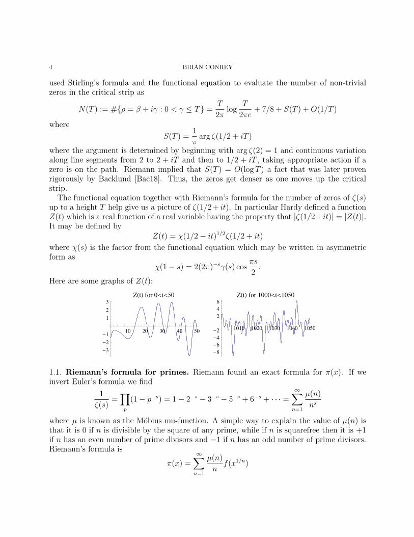
The functional equation together with Riemann’s formula for the number of zeros of ζ(s)up to a height T help give us a picture of ζ(1/2 + it). In particular Hardy defined a functionZ(t) which is a real function of a real variable having the property that |ζ(1/2+ it)| = |Z(t)|.It may be defined by
Z(t) = χ(1/2− it)1/2ζ(1/2 + it)
where χ(s) is the factor from the functional equation which may be written in asymmetricform as
χ(1− s) = 2(2π)−sγ(s) cosπs
2.
Here are some graphs of Z(t):
10 20 30 40 50
-3
-2
-1
1
2
3
ZHtL for 0<t<50
1010 1020 1030 1040 1050
-8
-6
-4
-2
2
4
6
ZHtL for 1000<t<1050
1.1. Riemann’s formula for primes. Riemann found an exact formula for π(x). If weinvert Euler’s formula we find
1
ζ(s)=∏p
(1− p−s) = 1− 2−s − 3−s − 5−s + 6−s + · · · =∞∑n=1
µ(n)
ns
where µ is known as the Mobius mu-function. A simple way to explain the value of µ(n) isthat it is 0 if n is divisible by the square of any prime, while if n is squarefree then it is +1if n has an even number of prime divisors and −1 if n has an odd number of prime divisors.Riemann’s formula is
π(x) =∞∑n=1
µ(n)
nf(x1/n)

RIEMANN’S HYPOTHESIS 5
where
f(x) = li(x)−∑ρ
li(xρ)− ln 2 +
∫ ∞x
dt
t(t2 − 1) log t.
Here the ρ = β+ iγ are the zeros of ζ(s) and the sum over the ρ is to be taken symmetrically,i.e. to pair the zero ρ with its dual 1−ρ as the sum is performed. Thus the difference betweenRiemann’s formula and Gauss’ conjecture is, to a first estimation, about li(xβ0) where β0 isthe largest or the supremum of the real parts of the zeros. Riemann conjectured that all ofthe zeros have real part β = 1/2 so that the error term is of size x1/2 log x. This assertion ofthe perfect balance of the zeros, and so of the primes, is Riemann’s Hypothesis.
In 1896 Hadamard and de la Vallee Poussin independently proved that ζ(1 + it) 6= 0 andconcluded that
π(N) ∼ li(N)
a theorem which is known as the prime number theorem.
2. Riemann and the zeros
After his evaluation of N(T ) ∼ T2π
log T he asserted that we find about this many realzeros of
Ξ(t) := ξ(1/2 + it)
in 0 < t ≤ T . This is an assertion which is still unproven and is the subject of speculation.His memoir “Ueber die Anzahl der Primzahlen unter einer gegebenen Grosse” is only 8 pages.But in the early 1930s his Nachlass was delivered from the library at Gottingen to Princetonwhere C. L. Siegel [?] looked over Riemann’s notes at the Institute for Advanced Study. Inthe notes were found an “approximate functional” equation, which had been independentlyfound by Hardy and Littlewood [HL29]:
ζ(s) =∑n≤ t
2π
1
ns+ χ(s)
∑n≤ t
2π
1
n1−s +O(t−σ/2)
for s = σ + it. Here χ(s) is the factor from the asymmetric form of the functional equation
ζ(s) = χ(s)ζ(1− s)with
χ(s) =π−(1−s)/2Γ((1− s)/2)
π−s/2Γ(s/2)= 2(2π)s−1Γ(1− s) sin
πs
2.
Now |χ(1/2 + it)| = 1; in fact χ(1/2 + it) = eit log t/2π(1 + O(1/t)). One might be led tobelieve that 1 + χ(s) is a reasonable approximation to ζ(s), i.e. that the contributions fromthe oscillatory terms 2−s etc. might be small overall. This approximation has zeros ons = 1/2 + it at a rate sufficient to produce asymptotically all of the zeros of ζ(s), so itseems reasonable to conclude that almost all of the zeros are on this line, and to go on andconjecture that ALL of the zeros are on the one-line. But we have found it hard to makethis reasoning precise.

6 BRIAN CONREY
Riemann computed the first few zeros:
1/2 + i14.13 . . . , 1/2 + i21.02 . . . , 1/2 + i25.01 . . . , . . .
A good way to be convinced that these are indeed zeros is to use the easily proven formula
(1− 21−s)ζ(s) = 1− 1
2s+
1
3s− 1
4s± . . . .
The alternating series on the right converges for <s > 0 and so, for example,
s = 1/2 + i14.1347251417346937904572519835624 . . .
can be substituted into a truncation of this series (using a computer algebra system) to seethat it is very close to 0. (See www.lmfdb.org to find a list of high precision zeros of ζ(s) aswell as a wealth of information about ζ(s) and similar functions called L-functions.)
3. Elementary equivalents of the Riemann Hypothesis
We’ve mentioned that the Riemann Hypothesis implies a good error bound for the primenumber theorem. The converse is also true: the Riemann Hypothesis is equivalent to
π(x) :=∑p≤x
1 =
∫ x
2
du
log u+O(x1/2 log x),
and to
ψ(x) :=∑pk≤x
log p = x+O(x1/2 log2 x)
Equivalences may also be phrased in terms of the Mobius function µ(n) where
1
ζ(s)=∞∑n=1
µ(n)
ns.
It is not difficult to show that the Riemann Hypothesis is equivalent to the assertion thatthis series is (conditionally) convergent for any s with 1/2 < σ < 1.
The Riemann Hypothesis is also equivalent to each of
M(x) :=∑n≤x
µ(n) = O(x1/2+ε)
and ∫ X
1
(ψ(x)− x)2dx
x2∼ C logX.
The assertion that ∫ X
1
M(x)2dx
x2∼ C logX
implies the Riemann Hypothesis and that all of the zeros are simple. A question is whetherthe converse is true.
RIEMANN’S HYPOTHESIS 7
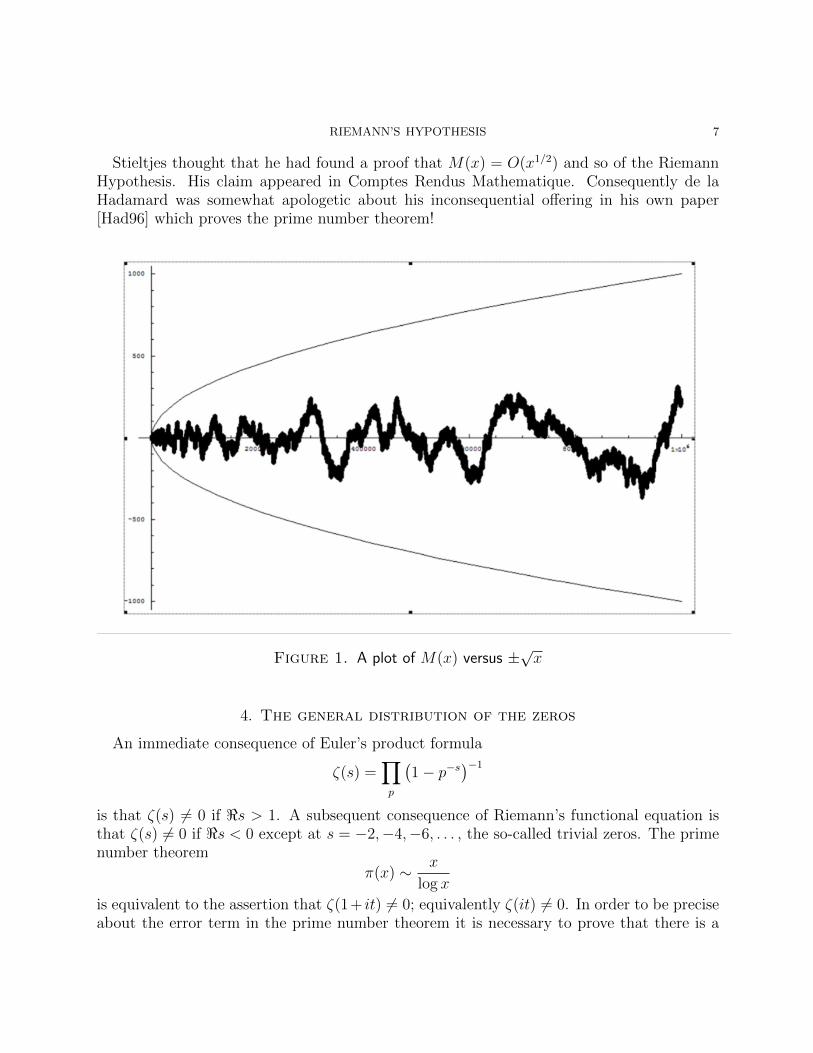
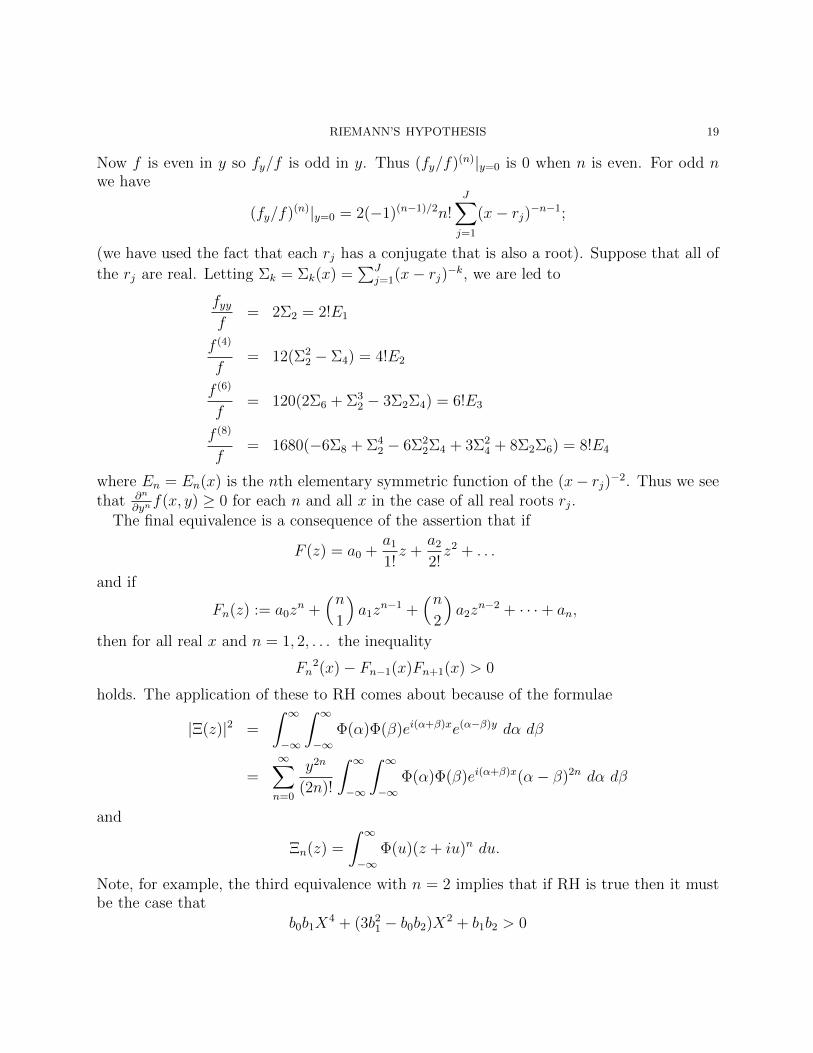
Stieltjes thought that he had found a proof that M(x) = O(x1/2) and so of the RiemannHypothesis. His claim appeared in Comptes Rendus Mathematique. Consequently de laHadamard was somewhat apologetic about his inconsequential offering in his own paper[Had96] which proves the prime number theorem!
Figure 1. A plot of M(x) versus ±√x
4. The general distribution of the zeros
An immediate consequence of Euler’s product formula
ζ(s) =∏p
(1− p−s
)−1
is that ζ(s) 6= 0 if <s > 1. A subsequent consequence of Riemann’s functional equation isthat ζ(s) 6= 0 if <s < 0 except at s = −2,−4,−6, . . . , the so-called trivial zeros. The primenumber theorem
π(x) ∼ x
log x
is equivalent to the assertion that ζ(1+ it) 6= 0; equivalently ζ(it) 6= 0. In order to be preciseabout the error term in the prime number theorem it is necessary to prove that there is a
8 BRIAN CONREY
region near the line σ = 1 in which there are no zeros. It was shown by de la Vallee Poussinin 1899 [Val96] that
ζ(σ + it) 6= 0
for σ > clog(2+|t|) for a specific c. This is known as a zero-free region. The best known shape
of the zero-free region is due to Korobov [Kor58] and Vinogradov [Vin58] in 1958: ζ(σ + it)is free of zeros when
σ > 1− C
(log t)2/3(log log t)1/3.
The best explicit value of C is due to Kevin Ford [For00] who showed that C = 1/54.57 isadmissible.
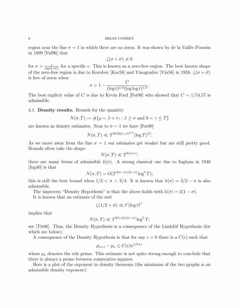
4.1. Density results. Bounds for the quantity
N(σ, T ) := #ρ = β + iγ : β ≥ σ and 0 < γ ≤ T
are known as density estimates. Near to σ = 1 we have [For00]
N(σ, T ) T 58.05(1−σ)3/2(log T )15.
As we move away from the line σ = 1 our estimates get weaker but are still pretty good.Bounds often take the shape
N(σ, T ) T k(σ)+ε;
there are many forms of admissible k(σ). A strong classical one due to Ingham in 1940[Ing40] is that
N(σ, T ) = O(T 3(1−σ)/(2−σ) log5 T );
this is still the best bound when 1/2 < σ < 3/4. It is known that k(σ) = 3/2 − σ is alsoadmissible.
The unproven “Density Hypothesis” is that the above holds with k(σ) = 2(1− σ).It is known that an estimate of the sort
ζ(1/2 + it) tc(log t)c′
implies that
N(σ, T ) T 2(1+2c)(1−σ) log5 T ;
see [Tit86]. Thus, the Density Hypothesis is a consequence of the Lindelof Hypothesis (forwhich see below).
A consequence of the Density Hypothesis is that for any ε > 0 there is a C(ε) such that
pn+1 − pn ≤ C(ε)n1/2+ε
where pn denotes the nth prime. This estimate is not quite strong enough to conclude thatthere is always a prime between consecutive squares.
Here is a plot of the exponent in density theorems (the minimum of the two graphs is anadmissible density exponent):
RIEMANN’S HYPOTHESIS 9
0.5 0.6 0.7 0.8 0.9
1.5
2.5
3
3.5
4
4.5
Density exponent kHsigmaL
4.2. Zeros near the 1/2-line. It has been known for quite some time that almost all ofthe zeros are near the 1/2-line. For example at least 99% of the zeros ρ = β + iγ satisfy
|β − 1/2| < 8
log γ.
and almost all are within φ(γ)/ log γ of the critical line where φ is any function which goesto infinity. Thus, we know that the zeros cluster around the critical line.
4.3. Zeros on the critical line. Many people have worked on verifying the Riemann Hy-pothesis. Today it is known that the first ten trillion zeros are all on the critical line<s = 1/2!
Hardy was the first one to show that there are infinitely many zeros on the 1/2-line. Heand Littlewood [HL18] later gave proofs that the number of zeros on the 1/2-line up to aheight T is more than a positive constant times T . In 1942 Selberg [Sel42] proved that apositive proportion of the zeros are on the critical line. In 1973 N. Levinson [Lev74] provedthat at least 1/3 of the zeros are on the half-line. This was improved in 1989 to at least 2/5of the zeros are on the line. The current record is Feng [Fen12] with 0.412; for simple zerosthe record proportion is due to Bui, Conrey, and Young [BCY11] who show that at least0.405 of the zeros of ζ(s) are on the critical line and simple.
It follows from the Riemann Hypothesis that all of the zeros of all of the derivatives ξ(k)(s)are on the critical line. Along these lines it can be shown, for example, that more than 4/5of the zeros of ξ′(s) are on the critical line and more than 99% of the zeros of ξ(5)(s) are onthe critical line, see [Con83].
5. The Lindelof Hypothesis
The assertion that for any ε > 0,
ζ(1/2 + it)ε tε
is known as the Lindelof Hypothesis and is a consequence of the Riemann Hypothesis. It isa consequence of the functional equation, trivial bounds for ζ(it) and ζ(1 + it), and general
10 BRIAN CONREY
principles of the growth of analytic functions that
ζ(1/2 + it)ε t14
+ε;
this is known as the convexity bound. Weyl, using exponential sums, improved the boundto
ζ(1/2 + it)ε t16
+ε.
Bombieri and Iwaniec [BI86] used some novel ideas to show
ζ(1/2 + it) t89/560+ε.
Huxley [Hux05] obtained
ζ(1/2 + it) t32/205 logc t.
Recently Bourgain [Bou14] announced that
ζ(1/2 + it) t53/342+ε
5.1. Estimates for ζ(s) near the 1-line. Richert [Ric67] proved the important estimatethat for an explicit c > 0,
|ζ(σ + it)| < ct100(1−σ)3/2 log2/3 t
for 1/2 ≤ σ ≤ 1, t ≥ 2. Such a bound is useful for zero-free regions, the error term in theprime number theorem, and zero density results near 1. K. Ford [For02] has improved thesemade the constants explicit:
|ζ(σ + it)| < 76.2t4.45(1−σ)3/2 log2/3 t.
5.2. 1 versus 2. RH implies that
|ζ(1/2 + it)| exp
(log 2
2
log t
log log t+O
(log t log log | log t
(log log t)2
))see [ChS11] . It can be proven, see [Sou08] that every interval [T, 2T ] contains a t for which
|ζ(1/2 + it)| ≥ exp
((1 + o(1))
(log t)1/2
(log log t)1/2
).
Which of these is closer to the true largest order of magnitude of ζ on the 1/2-line? It isdifficult to say, though most people (not the author!) think that the lower bound (Ω-result)is closer to the truth. Farmer, Gonek, and Hughes [FGH07] conjecture that
|ζ(1/2 + it)| ≤ exp
(√(1
2+ o(1)
)(log t)(log log t)
).
RIEMANN’S HYPOTHESIS 11
6. Computations
Turing was the first to use a computer to calculate the zeros of ζ(s). He proposed anefficient rigorous method to verify RH up to a given height, or indeed within an interval.It involves using a precise version of the approximate functional equation, known as theRiemann - Siegel formula, to evaluate Z(t) and detect sign changes, together with an explicitbound for the average of S(t) namely if t2 > t1 > 168π then∫ t2
t1
S(t) dt = Θ
(2.30 + 0.128 log
t22π
)to verify that all of the zeros are accounted for. (Here Θ represents a number that is at most1 in absolute value.) Goldfeld has pointed out that if ζ(s) had a double zero somewhereup the line, the computational verification of RH would come to a halt because it would beimpossible to distinguish a double zero from two very close zeros either on or off the line.
Here is one of Turing’s versions of the Riemann-Siegel formula:
Theorem 1. Let m and ξ be respectively the integral and non-integral parts of τ 1/2 and
τ ≥ 64,
κ(τ) =1
4πilog
Γ(14
+ πiτ)
Γ(14− πiτ)
− 1
4τ log π,
Z(τ) = ζ(1/2 + 2πiτ)e−2πκ(τ),
κ1(τ) =1
2(τ log τ − τ − 1
2),
h(ξ) =cos 2π(ξ2 − ξ − 1
16)
cos 2πξ.
Then Z(τ) is real and
Z(τ) = 2m∑n=1
n−12 cos 2πτ log n− κ(τ)+ (−1)m+1τ−
14h(ξ) + Θ(1.09τ−
34 ,
κ(τ) = κ1(τ) + Θ(0.006τ−1).
In 1988, Andrew Odlyzko and Schonhage [OS88] invented an algorithm which allowed forthe very speedy calculation of many values of ζ(s) at once. The Riemann-Siegel allows fora single computation of ζ(1/2 + it) with T < t < T + T 1/2 in time T 1/2+ε. The Odlyzko -Schonhage algorithm allows for a single computation in time T ε after a pre-computation oftime T 1/2+ε. This led Odlyzko to compile extensive statistics about the zeros at enormousheights - up to 1023 and higher. His famous graphs showed an incredible match betweendata for zeros of ζ(s) and for the proven statistical distributions for random matrices.
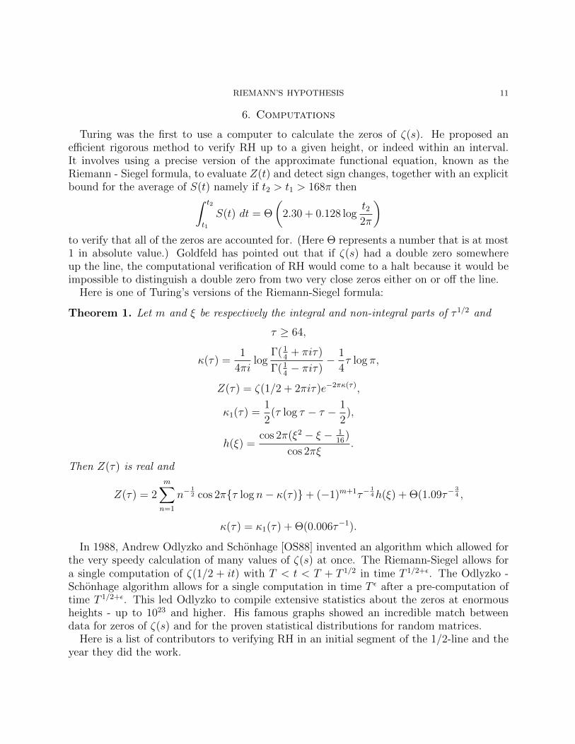
Here is a list of contributors to verifying RH in an initial segment of the 1/2-line and theyear they did the work.
12 BRIAN CONREY
G. H. B. Riemann 3 1859J. P. Gram 15 1903R. J. Backlund 79 1914E. C. Titchmarsh 1041 1935A. M. Turing 1104 1953D. H. Lehmer 15000 1956D. H. Lehmer 25000 1956N. A. Meller 35337 1958R S. Lehman 250000 1966J. B. Rosser , J. M. Yohe, L. Schoenfeld 3500000 1968R. P. Brent 40000000 1977R. P. Brent 81000000 1979R. P. Brent, J. van de Lune, H. J. J. te Riele, D. T. Winter 200000001 1982J. van de Lune, H. J. J. te Riele 300000001 1983J. van de Lune, H. J. J. te Riele, D. T. Winter 1500000001 1986J. van de Lune 10000000000 2001S. Wedeniwski 900000000000 2004X. Gourdon, P. Demichel 10000000000000 2004
Ghaith Hiary [Hia11] has improved these algorithms. He can compute one value of ζ(1/2+it) in time T 1/3+ε using an algorithm that has been implemented by Jonathan Bober and
Hiary; he has a more complicated algorithm that will work in time T413
+ε. They have verifiedRH in some small ranges around the 1033 zero!
Bober’s website [Bob14] has some great pictures of large values of Z(t).
7. Why do we think RH is true?
The main reason is because of the beauty of the conjecture. It strikes our sensibilities asappropriate that something so incredibly symmetric should be true in mathematics. Thesecond reason is that the first 10 trillion zeros are all on the line. If there were a counterex-ample it should have shown itself by now. A third reason is that the numerical evidence forall L-functions ever computed lead to this conclusion; some have thought that a counterex-ample to RH might show itself when computing zeros of L-functions associated with Maassforms because these have no arithmetic-geometry interpretation (eg. their coefficients aregenerally believed to be transcendental); however the computations reveal that the zeros arestill on the 1/2-line. A fourth reason is probabilistic. RH is known to be equivalent to theassertion that M(x) :=
∑n≤x µ(n) x1/2 log2 x. This sum represents the difference between
the number of squarefree integers up to x with an even number of prime factors and thenumber with an odd number of prime factors. It is similar to the difference in the numberof heads and tails when one flips x coins, and so should be around x1/2.
Here is another more elaborate reason. Suppose that a Dirichlet series F (s) =∑∞
n=1 ann−s
converges for σ > 0, and suppose that it has a zero with real part β > 1/2. We mightreasonably expect it then to have T zeros in σ > β − ε, 0 < t < T for any large T by
RIEMANN’S HYPOTHESIS 13
“almost periodicity.” But zero density results tell us that there are T 1−δ zeros in σ ≥ σ0
and t < T .
7.1. Almost periodicity. As just mentioned a possible strategy is to try to prove that ifζ(s) has one zero off the line then it has infinitely many off the line. Bombieri [Bom00] hascome closest to achieving this.
Here is a conjecture that attempts to encapsulate this idea:
Conjecture 1. Suppose that the Dirichlet series
F (s) =∞∑n=1
ann−s
converges for σ > 0 and has a zero in the half-plane σ > 1/2. Then there is a number CF > 0such that F (s) has > CFT zeros in σ > 1/2, |t| ≤ T .
This seemingly innocent conjecture implies the Riemann Hypothesis for virtually anyprimitive L-function (except curiously possibly the Riemann zeta-function itself!). And itseems that the Euler product condition has already been used (in the density result above);i.e. the hard part is already done. Note that the “1/2” in the conjecture needs to be thereas the example
∞∑n=1
µ(n)/n1/2
ns
demonstrates. Assuming RH, this series converges for σ > 0 and its lone zero is at s = 1/2.This example is possibly at the boundary of what is possible.
8. A spectral interpretation
Hilbert and Polya are reputed to have suggested that the zeros of ζ(s) should be interpretedas eigenvalues of an appropriate operator.
Odlyzko wrote to Polya to ask about this. Here is the text of Odlyzko’s letter, dated Dec.8, 1981.
Dear Professor Polya:I have heard on several occasions that you and Hilbert had independently conjectured
that the zeros of the Riemann zeta function correspond to the eigenvalues of a self-adjointhermitian operator. Could you provide me with any references? Could you also tell mewhen this conjecture was made, and what was your reasoning behind this conjecture atthat time?
The reason for my questions is that I am planning to write a survey paper on the dis-tribution of zeros of the zeta function. In addition to some theoretical results, I haveperformed extensive computations of the zeros of the zeta function, comparing their dis-tribution to that of random hermitian matrices, which have been studied very seriouslyby physicists. If a hermitian operator associated to the zeta function exists, then in somerespects we might expect it to behave like a random hermitian operator, which in turn ughtto resemble a random hermitian matrix. I have discovered that the distribution of zeros of
14 BRIAN CONREY
the zeta function does indeed resemble the distribution of eigenvalues of random hermitianmatrices of unitary type.
Any information or comments you might care to provide would be greatly appreciated.
Sincerely yours,
Andrew Odlyzko
and Polya’s response, dated January 3, 1982.
Dear Mr. Odlyzko,Many thanks for your letter of Dec. 8. I can only tell you what happened to me.I spent two years in Gottingen ending around the beginning of 1914. I tried to learn
analytic number theory from Landau. He asked me one day: “You know some physics. Doyou know a physical reason that the Riemann Hypothesis should be true?”
This would be the case, I answered, if the non-trivial zeros of the ζ function were soconnected with the physical problem that the Riemann Hypothesis would be equivalent tothe fact that all the eigenvalues of the physical problem are real.
I never published this remark, but somehow it became known and it is still remembered.
With best regards.
Yours sincerely,
George, Polya
9. The vertical spacing of zeros
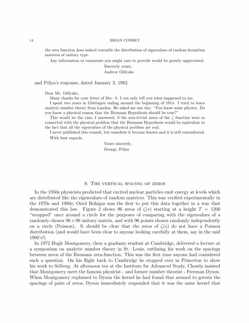
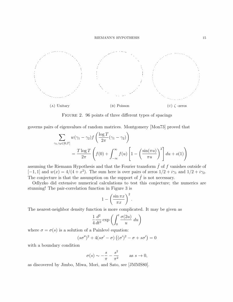
In the 1950s physicists predicted that excited nuclear particles emit energy at levels whichare distributed like the eigenvalues of random matrices. This was verified experimentally inthe 1970s and 1980s; Oriol Bohigas was the first to put this data together in a way thatdemonstrated this law. Figure 2 shows 96 zeros of ζ(s) starting at a height T = 1200“wrapped” once around a circle for the purposes of comparing with the eigenvalues of arandomly chosen 96×96 unitary matrix, and with 96 points chosen randomly independentlyon a circle (Poisson). It should be clear that the zeros of ζ(s) do not have a Poissondistribution (and would have been clear to anyone looking carefully at them, say in the mid1900’s!).
In 1972 Hugh Montgomery, then a graduate student at Cambridge, delivered a lecture ata symposium on analytic number theory in St. Louis, outlining his work on the spacingsbetween zeros of the Riemann zeta-function. This was the first time anyone had consideredsuch a question. On his flight back to Cambridge he stopped over in Princeton to showhis work to Selberg. At afternoon tea at the Institute for Advanced Study, Chowla insistedthat Montgomery meet the famous physicist - and former number theorist - Freeman Dyson.When Montgomery explained to Dyson the kernel he had found that seemed to govern thespacings of pairs of zeros, Dyson immediately responded that it was the same kernel that
RIEMANN’S HYPOTHESIS 15
(a) Unitary (b) Poisson (c) ζ -zeros
Figure 2. 96 points of three different types of spacings
governs pairs of eigenvalues of random matrices. Montgomery [Mon73] proved that∑γ1,γ2∈[0,T ]
w(γ1 − γ2)f
(log T
2π(γ1 − γ2)
)
=T log T
2π
(f(0) +
∫ ∞−∞
f(u)
[1−
(sin(πu)
πu
)2]du+ o(1)
)assuming the Riemann Hypothesis and that the Fourier transform f of f vanishes outside of[−1, 1] and w(x) = 4/(4 + x2). The sum here is over pairs of zeros 1/2 + iγ1 and 1/2 + iγ2.
The conjecture is that the assumption on the support of f is not necessary.Odlyzko did extensive numerical calculations to test this conjecture; the numerics are
stunning! The pair-correlation function in Figure 3 is
1−(
sinπx
πx
)2
.
The nearest-neighbor density function is more complicated. It may be given as
1
4
d2
dt2exp
(∫ t
0
σ(2u)
udu
)where σ = σ(s) is a solution of a Painleve equation:
(sσ′′)2 + 4(sσ′ − σ)((σ′)2 − σ + sσ′
)= 0
with a boundary condition
σ(s) ∼ − sπ− s2
π2as s→ 0,
as discovered by Jimbo, Miwa, Mori, and Sato, see [JMMS80].
16 BRIAN CONREY
(a) Pair correlation (b) Nearest neighbor
Figure 3. Odlyzko’s graphics
Now we have the challenge of not only explaining why all of the zeros are on a straightline, but also why they are distributed on this line the way they are! The connections withRandom Matrix theory first discovered by Montgomery and Dyson have received a greatdeal of support from seminal papers of Katz and Sarnak [KaSa99] and Keating and Snaith[KS00]. The last 15 years have seen an explosion of work around these ideas. In particular,it definitely seems like there should be a spectral interpretation of the zeros a la Hilbert andPolya.
10. Some initial thoughts about proving RH
10.1. Fourier integrals with all real zeros. Riemann proved that
Ξ(t) := ξ(1/2 + it) =
∫ ∞−∞
Φ(u)eiut du
where
Φ(u) =∞∑n=1
(4π2n4e9u/2 − 6n2πe5u/2) exp(−n2πe2u)
It is known that Φ(u) is even, is positive for real u and is (rapidly!) decreasing for u > 0.Consequently, we can write
Ξ(t) = 2
∫ ∞0
Φ(u) cosut du
=∞∑n=0
(−1)nbn(2n)!
t2n
RIEMANN’S HYPOTHESIS 17
where
bn :=
∫ ∞−∞
Φ(u)u2n du.
The Riemann Hypothesis is the assertion that all of the zeros of Ξ(t) are real. This hasprompted investigations into Fourier integrals with all real zeros. Polya [Pol27] and deBruijn[deB50] spent a lot of time with such investigations. A sample theorem is
Theorem 2. Let f(u) be an even nonconstant entire function of u, f(u) ≥ 0 for real u, andsuch that f ′(u) = exp (γu2)g(u), where γ ≥ 0 and g(u) is an entire function of genus ≤ 1with purely imaginary zeros only. Then Ψ(z) =
∫∞−∞ exp −f(u)eizudt has real zeros only.
Now Φ(u) > 0 for all real u and Φ′(u) < 0 for u ≥ 0. Thus, we can write Φ(u) = e−f(u).The functional equation for ζ(s) is equivalent to the assertion that Φ(u) is even.
In particular, it was shown by Polya [Pol26] that all of the zeros of the Fourier transformof a first approximation Φ∗(u) to Φ(u)
Φ∗(u) = (2π cosh(9u/2)− 3 cosh 5u/2) exp(−2π cosh 2u)
are real. These ideas have been further explored by deBruijn, Newman [New76], Hejhal,Haseo Ki [KK02], [KK03] and others. Hejhal [Hej90] has shown that almost all of the zerosof the Fourier transform of any partial sum of Φ(u) are real.
A goal of this approach is to determine necessary and sufficient conditions that describethe Fourier transform of a function all of whose zeros are real.
10.2. Jensen’s inequalities. In section 14.32 of [Tit86], we find the assertion that RH isequivalent to ∫ ∞
−∞
∫ ∞−∞
Φ(α)Φ(β)ei(α+β)xe(α−β)y(α− β)2 dα dβ ≥ 0
for all real x and y where Φ(u) is as in the last section.We quote a passage from Polya’s collected works, volume I, page 427, written by M.
Marden commenting on the paper of Polya.
In this paper Professor Polya reports his findings on examining the “Nachlass”of the Danish mathematician J. L. W. V. Jensen who died in 1925. Fourteenyears earlier Jensen had announced that he would publish a paper regardinghis algebraic-function theoretic research on the Riemann ξ-function. In view ofJensen’s well-known interest in the zeros of polynomials and entire functions,expectations were high that Jensen would contribute to the solution of theRiemann hypothesis problem regading the zeros of the ξ-function. However,this paper was never published, and so on Jensen’s death it was a matterof paramount importance to have his papers examined by an expert in thisarea. Professor Polya undertook this task, but after an arduous examinationhe found no clue to any progress that Jensen may have made towards theRiemann hypothesis.
18 BRIAN CONREY
Professor Polya does sketch Jensen’s algebraic-function-theoretic investiga-tions, many of which were advanced considerably by Polya’s own work.
In this paper, Polya gives two more necessary and sufficient conditions for RH. RH isequivalent to ∫ ∞
−∞
∫ ∞−∞
Φ(α)Φ(β)ei(α+β)x(α− β)2n dα dβ ≥ 0
for all real values of x and n = 0, 1, 2, . . . ; and finally RH is equivalent to∫ ∞−∞
∫ ∞−∞
Φ(α)Φ(β)(x+ iα)n(x+ iβ)n(α− β)2 dα dβ ≥ 0
for all real values of x and n = 0, 1, 2, . . . .Polya points out that the first equivalence to RH follows immediately from the more
general theorem that all of the zeros of a real entire function F (z) of genus at most 1 arereal if and only if
∂2
∂y2|F (z)|2 ≥ 0
for all z = x + iy. To see that this condition is necessary for polynomials suppose thatF (z) =
∏Jj=1(z − rj) and let f(x, y) = |F (z)|2. Then log f =
∑Jj=1 log(z − rj) + log(z − rj)
so that
fyf
=J∑j=1
(i
z − rj− i
z − rj
)= 2
J∑j=1
=(z − rj)|z − rj|2
.
Taking another partial with respect to y leads to
fyy − (fy)2
f 2=
J∑j=1
(1
(z − rj)2+
1
(z − rj)2
)= 2
J∑j=1
<(z − rj)2
|z − rj|4.
If all of the rj are real we have
fyyf
= 4y2
(J∑j=1
1
|z − rj|2
)2
+ 2J∑j=1
(x− rj)2
|z − rj|4− 2y2
J∑j=1
1
|z − rj|4.
The middle term is clearly positive and the first term is clearly greater than 4y2∑J
j=11
|z−rj |4
which is twice the third term in absolute value. Thus the condition is necessary.The second equivalent to RH is a consequence of the fact that if for each real x the function
f(x, y) = |F (x+ iy)|2 is expanded into a power series in y then all of the coefficients shouldbe non-negative. To see this, again for polynomials, let the notation be as above. We have(
∂
∂y
)n(fyf
)∣∣∣∣y=0
= in−1n!J∑j=1
(1
(z − rj)n+1+
(−1)n+1
(z − rj)n+1
).
RIEMANN’S HYPOTHESIS 19
Now f is even in y so fy/f is odd in y. Thus (fy/f)(n)|y=0 is 0 when n is even. For odd nwe have
(fy/f)(n)|y=0 = 2(−1)(n−1)/2n!J∑j=1
(x− rj)−n−1;
(we have used the fact that each rj has a conjugate that is also a root). Suppose that all of
the rj are real. Letting Σk = Σk(x) =∑J
j=1(x− rj)−k, we are led to
fyyf
= 2Σ2 = 2!E1
f (4)
f= 12(Σ2
2 − Σ4) = 4!E2
f (6)
f= 120(2Σ6 + Σ3
2 − 3Σ2Σ4) = 6!E3
f (8)
f= 1680(−6Σ8 + Σ4
2 − 6Σ22Σ4 + 3Σ2
4 + 8Σ2Σ6) = 8!E4
where En = En(x) is the nth elementary symmetric function of the (x− rj)−2. Thus we seethat ∂n
∂ynf(x, y) ≥ 0 for each n and all x in the case of all real roots rj.
The final equivalence is a consequence of the assertion that if
F (z) = a0 +a1
1!z +
a2
2!z2 + . . .
and if
Fn(z) := a0zn +
(n1
)a1z
n−1 +(n
2
)a2z
n−2 + · · ·+ an,
then for all real x and n = 1, 2, . . . the inequality
Fn2(x)− Fn−1(x)Fn+1(x) > 0
holds. The application of these to RH comes about because of the formulae
|Ξ(z)|2 =
∫ ∞−∞
∫ ∞−∞
Φ(α)Φ(β)ei(α+β)xe(α−β)y dα dβ
=∞∑n=0
y2n
(2n)!
∫ ∞−∞
∫ ∞−∞
Φ(α)Φ(β)ei(α+β)x(α− β)2n dα dβ
and
Ξn(z) =
∫ ∞−∞
Φ(u)(z + iu)n du.
Note, for example, the third equivalence with n = 2 implies that if RH is true then it mustbe the case that
b0b1X4 + (3b2
1 − b0b2)X2 + b1b2 > 0
20 BRIAN CONREY
for all real X where we are using the notation
bn =
∫ ∞−∞
Φ(u)u2n du
from above. This inequality holds in turn if the discriminant of the quadratic in X2 isnegative:
9b41 − 10b2
0b1b2 + b20b
22 < 0
i.e.
(9b21 − b0b2)(b2
1 − b0b2) < 0.
A consequence is that b0b2 < 9b21. (The Turan inequalities, see below, imply that 3b2
1 > b0b2,that 5b2
2 > 3b1b3, that 7b23 > 5b2b4 etc. and Cauchy’s inequality implies that b2
n ≤ bn−abn+a
for a = 1, 2, . . . , n so in particular
3b21 > b0b2 > b2
1.
In fact it is easily calculated that the ratio b0b2b21
= 2.79 . . . . Note that the Karlin-Nuttall
inequality below would have this ratio smaller than 6. )For n = 3 the Jensen inequality implies that
b0b1X6 + (6b2
1 − 3b0b2)X4 + 3b1b2X2 + b2
2 > 0
for all X. The discriminant of this cubic in X2 is
−746496b0b62
(b3
0b32 − 7b2
0b21b
22 + 11b0b
41b2 − 5b6
1
)2< 0
so that the cubic has only one real root. Since the value at x = 0 is positive, the real rootis negative and so the third Jensen inequality is always true. For n = 4 the condition is
b0b1X8 + (10b2
1 − 6b0b2)X6 + (5b1b2 + b0b3)X4 + (10b22 − 6b1b3)X2 + b2b3 > 0
for all X.
11. Grommer inequalities
In 1914 Grommer [Gro14] found a necessary and sufficient condition for the reality of thezeros of an entire function. We describe how it applies to the Riemann Hypothesis. LetΞ(t) = ξ(1/2+ it) so that RH is the assertion that all zeros of Ξ are real. Now the functionalequation for ζ is equivalent to the fact that Ξ(t) is even. Let Y (t) = Ξ(
√t) and let
−Y′
Y(t) = s1 + s2t+ s3t
2 + . . . .
Then RH is equivalent to the assertion that for each n,
Dn = det
s2 s3 . . . sn+1
s3 s4 . . . sn+2...
......
sn+1 sn+2 . . . s2n
> 0.
RIEMANN’S HYPOTHESIS 21
The collection of inequalities for n = 1 applied to Y (t) = Ξ(√t) and all of its derivatives are
sometimes known as the Turan inequalities.Here is a proof of the necessity of Grommer’s criterion. First off we consider the polynomial
case. Assume that P is a polynomial with P (0) 6= 0. Let
P (z) =n∏r=1
(z − 1/zr)
be a polynomial with real coefficients.We have
P ′
P(z) =
n∑r=1
1
z − 1/zr= −
n∑r=1
zr1− zzr
= −n∑r=1
∞∑m=0
zmzrm+1
so that
−P′
P(z) = s1 + s2z + s3z
2 + . . .
where
sm =n∑r=1
zmr
is the sum of the mth powers of the reciprocal roots. Let Dm be the m × m Grommerdeterminant as above. The key observation is that
Dn = ∆(z1, . . . , zn)2
n∏r=1
z2r
where ∆ is the Vandermonde determinant for which we have the formula
∆(z1, . . . , zn) =∏
1≤i<j≤n
(zj − zi).
More generally, if m ≤ n, then
Dm =∑
Z⊂z1,...,zn|Z|=m
( ∏zr∈Z
z2r
)∆(Z)2
and Dm = 0 if m > n. (Note that whereas ∆(Z) has an ambiguous sign, the notation ∆(Z)2
makes sense.) Thus, it is clear that if all of the zr are real, then all of the Dm ≥ 0, soGrommer’s condition is a necessary condition for the reality of the zeros of P .
We can show that the condition is sufficient if there are an odd number of conjugate pairsof non-real zeros. If only one pair, say z1, z2 with z2 = z1 is complex, and all of the rest aredistinct reals, then
Dn = |z1|2n∏r=3
z2r∆(z3, . . . , zn)2(z1 − z2)2
n∏r=3
|zr − z1|2.

22 BRIAN CONREY
All of the factors here are positive with the exception of (z1 − z2)2 = −4(=z1)2 < 0. Thus,Dn < 0. The same argument works anytime there are an odd number of pairs of complexzeros.
If there are an even number of pairs of non-real complex conjugate pairs of zeros, say mof them, then it seems that Dn−m < 0 but we don’t see how to prove this.
Grommer’s argument proceeds via the Euler-Stieltjes theory of continued fractions, whichstudy contains the genesis of the theory of orthogonal polynomials.
The second set of Grommer inequalities asserts that
10b20b2b4 − 21b2
0b23 − 30b0b
21b4 + 350b0b1b2b3 − 350b0b
32 − 420b3
1b3 + 525b21b
22 > 0.
12. Turan inequalities
The entire function Ξ(t) can be expanded into an everywhere convergent power series:
Ξ(t) =∞∑n=0
(−1)nbnt2n
(2n)!
where
bn =
∫ ∞−∞
Φ(u)u2n du.
Let
Y (t) = Ξ(√t) =
∞∑n=0
(−1)nbntn
(2n)!.
Then Y is entire of order 1/2 and the Riemann Hypothesis implies that all of its zeros arereal, and in addition, that all of the zeros of all derivatives Y (m)(t) are real. From theGrommer inequalities, a necessary condition for all of the zeros of Y (t) to be real is thats2 > 0 where
−Y′
Y(t) = s1 + s2t
2 + s3t3 + . . . ;
in other words (Y ′
Y
)′(0) < 0.
Thus, RH implies that (Y (m+1)
Y (m)
)′(0) < 0
for m = 0, 2, 4, . . . . It is easy to check that this condition translates to
b2m >
2m− 1
2m+ 1bm−1bm+1 (m = 1, 2, . . . );
these are known as the Turan inequalities and give a necessary but not sufficient conditionfor the reality of all of the zeros of Ξ(t). Matiyasevich [Mat82] and Csordas, Norfolk, and
RIEMANN’S HYPOTHESIS 23
Varga [CNV86] proved the Turan inequalities for Ξ. Conrey and Ghosh [CoGh94] consideredthese for the ξ function associated with the Ramanujan τ -function.
In conjunction with this, they show
Theorem 3. Let F ∈ C3(R). Let F (u) be positive, even, and decreasing for positive u, andsuppose that F ′/F is decreasing and concave for u > 0. Suppose that F is rapidly decreasingso that
X(t) =
∫ ∞−∞
F (u)eitu du
is an entire function of t. Then X(t) satisfies the Turan inequalities.
12.1. Karlin and Nuttall. We let Φ(u) be Riemann’s function as earlier. We let
Ξ(t) =∞∑n=0
(−1)nbn
(2n)!t2n
where
bn =
∫ ∞−∞
Φ(u)u2n du
as before. Define
B(i, j) =
bj−i(2j−2i)!
if i ≤ j
0 if i > j
Then RH is equivalent to D(n, r) > 0 for all positive r and non-negative n where
D(n, r) = detr×r
B(i, j + n)|i,j=1,r
(see [Kar68] chapter 8). The case r = 1 here is clear since F (u) > 0. The case r = 2 isslightly weaker than the Turan inequalities; it asserts that
b2m >
m
m+ 1
(2m− 1)
(2m+ 1)bm−1bm+1.
Nuttall [Nut13] has established the case r = 3 which asserts that
b3m
((2m)!)3− 2bm−1bm+1bm
(2m)!(2m− 2)!(2m+ 2)!− bm−2bm+2bm
(2m)!(2m− 4)!(2m+ 4)!
+b2m−1bm+2
((2m− 2)!)2(2m+ 4)!+
bm−2b2m+1
(2m− 4)!((2m+ 2)!)2> 0
for all m ≥ 2. For m = 2 this is
b32 −
4
5b1b3b2 −
1
70b0b4b2 +
2
75b0b
23 +
3
35b2
1b4 > 0.
24 BRIAN CONREY
13. Turan inequalities, 2
Ramanujan’s tau-function may be defined by equating coefficients of the power series onboth sides of
∞∑n=1
τ(n)xn = x∞∏n=1
(1− xn)24
The associated Dirichlet series is
L(s) = Lτ (s) =∞∑n=1
τ(n)n−s
This series is absolutely convergent for σ = <s > 13/2. The xi-function for τ is given by
ξτ (s) = (2π)−sΓ(s)L(s)
and it satisfies the functional equation
ξτ (s) = ξτ (12− s).
This functional equation is equivalent to the fact that
∆(z) =∞∑n=1
τ(n)e(nz)
is a holomorphic cusp form of weight 12 for the full modular group which in turn is equivalentto: (i) ∆(z) is expressible in terms of a Fourier series in z in which coefficients of e(nz) withn ≤ 0 vanish and (ii) ∆ satisfies the transformation formula
∆(−1/z) = z12∆(z).
It is believed that all of the zeros of ξ(s) are on the line <s = 6; this is the RiemannHypothesis for Lτ . See Hardy [Har78], Chapter X for introductory information about τ .
Now
ξτ (s) =
∫ ∞0
∆(iy)ysdy
y
so that
Ξτ (t) = ξτ (6 + it) =
∫ ∞−∞
∆(ieu)e6ueiut du
is an entire even function of t. We define
Φτ (u) = ∆(ieu)e6u
We see that Φτ (u) is an even function of u by the functional equation for ξτ . The factthat Φτ (u) > 0 for real u is immediately obvious from the product formula for ∆:
Φτ (u) = e6ue−2πeu∞∏n=1
(1− e−2πneu
)24
RIEMANN’S HYPOTHESIS 25
We can also see that Φτ (u) is decreasing for positive u by calculating the logarithmic deriv-ative. We first observe that
yd
dy
∞∑n=1
log(1− yn) = −y ddy
∞∑m,n=1
ymn
m= −
∞∑m,n=1
nymn = −∞∑n=1
σ(n)yn
where
σ(n) =∑d|n
d
is the sum of divisors of n. Let x = 2πeu and y = e−x. Then
Φτ (u) = e6uy∞∏n=1
(1− yn)24
so that
Φ′τΦτ
(u) = 6 +
(1
y− 24
∞∑n=1
σ(n)yn
)dy
du
= 6− x(1− Σ0(x))
where
Σk(x) = 24∞∑n=1
nkσ(n)yn
(The expansion of Φ′τ/Φτ above is related to the Fourier expansion of the Eisenstein seriesE2:
E2(z) = 1− 24∞∑n=1
σ(n)e(nz)
E2 is not a modular form of weight 2; it transforms according to the formulae
E2(−1/z) = z2E2(z) +12z
2πi
and E2(z + 1) = E2(z). Note also that
P (y) = E2(e2y)
satisfies the Chazy equation
P ′′′ − 2PP ′′ + 3(P ′)2 = 0;
the Chazy equation is related to a Painleve equation.)Now Φ′τ/Φτ is an odd function of u so that Φ′τ/Φτ (0) = 0. Thus, to show that Φ′τ (u) < 0
for u > 0 it suffices to prove that (Φ′τΦτ
)′(u) < 0
26 BRIAN CONREY
for u > 0. But (Φ′τΦτ
)′(u) = (−1 + Σ0(x) + xΣ′0(x))
dx
du
= −x+ xΣ0(x)− x2Σ1(x)
since Σ′k(x) = −Σk+1(x) and this then is
= −x
(1− 24
∞∑n=1
σ(n)yn(1− nx)
)Since u ≥ 0 corresponds to x ≥ 2π each of the terms 1−nx < 0 so that the whole expressionis negative.
Arguing in the same way we see that (Φ′τΦτ
)′′(u)
is odd and (Φ′τΦτ
)′′′(u) = −x(x3Σ3(x)− 6x2Σ2(x) + 7xΣ1(x)− Σ0(x) + 1)
= −x(1− 24∞∑n=1
σ(n)ynP3(nx))
whereP3(x) = 1− 7x+ 6x2 − x3 < 0
for x > 6. Thus we conclude that (Φ′τΦτ
)′′(u) < 0
for u > 0, i.e. that Φ′τΦτ
is concave for u > 0; see [CoGh94] for more details.
13.1. A difficulty with classifying functions whose Fourier transforms have realzeros. Let
g(u) = −u4
+πeu
12+∞∑n=1
σ−1(n)e−2πneu .
Here σ−1(n) =∑
d|n d−1 is the sum of the reciprocals of the positive divisors of n.
Then g(u) is positive, even, decreasing, and its logarithmic derivative is decreasing andconcave for u > 0. So
Ξk(t) =
∫ ∞−∞
e−kg(u)eiut du
might seem to be a good candidate for a function to have only real zeros. In fact k = 24 is thecase we’ve just been discussing about the Ramanujan tau-function. And k = 1 correspondsto the Xi-function associated with the Dirichlet L-function associated to the unique primitivecharacter of modulus 12, and so all of its zeros should be real by the Riemann Hypothesis for
RIEMANN’S HYPOTHESIS 27
that L-function. We believe for k = 1, 2, 3, 4, 6, 8, 12, 24 that all of the zeros of Ξk(t) shouldbe real, and for all other values of k > 0 that there will be non-real zeros. In [CoGh94] it isproven that Ξ48 has non-real zeros.
This example illustrates a difficulty with trying to give conditions for a function f(u) tohave all of the zeros of its Fourier transform be real. Conditions only involving the positivityof linear combinations of products and quotients of f(u) and its derivatives will fail as thisexample shows.
By contrast, if f(t) is twice continuously differentiable, f(t) > 0, f ′(t) < 0, and f ′′(t) < 0for 0 ≤ t ≤ 1 then all of the zeros of the even entire function
F (z) =
∫ 1
0
f(t) cos zt dt
are real. See [PS98], Part V, problem 173.
14. Hardy and Littlewood, Riesz, Baez-Duarte
M. Riesz [Rie16] proved that RH is true if and only if
R(x) = x∞∑k=0
(−x)k
k!ζ(2k + 2) x1/4+ε
and Hardy and Littlewood showed that RH holds if and only if∞∑k=1
(−x)k
k!ζ(2k + 1) x−1/4.
To see Riesz’ theorem, observe that
R(x) =i
2
∫(3/4)
xs
Γ(s)ζ(2s) sinπsds =
−1
2πi
∫(3/4)
Γ(1− s)xs
ζ(2s)ds.
If RH is true we move the path of integration to (1/4 + ε) and obtain the upper bound.Conversely, if the upper bound is true, then by the inverse Mellin transform we have that
Γ(1− s)ζ(2s)
= −∫ ∞
0
R(x)x−1−s ds
is analytic for <s > 1/4 so that RH is true.In a somewhat similar vein, Baez-Duarte [B-D05] has shown that RH is equivalent to the
estimate
ck :=k∑j=0
(−1)j(kj
)ζ(2j + 2)
ε k−3/4+ε
He initially suggested that ckk3/4 log2 k might have a limit. However, further investigations
indicate that ck oscillates between ±ck−3/4 which, if true, implies that all of the zeros aresimple and on the one-half line.
28 BRIAN CONREY
An interesting feature is that, like the Riesz and the Hardy-Littlewood criteria, this condi-tion only involves values of ζ(s) to the right of the critical strip. The first mentioned criteriainvolve a whole interval of estimates whereas this is one estimate. Note also that an alternateformula for ck is
ck =∞∑n=1
µ(n)
n2
(1− 1
n2
)k.
Baez-Duarte remarks that it is easy to show that
|ck| ≤∞∑n=1
1
n2
(1− 1
n2
)k k−1/2
so that the representation
1
ζ(s)=∞∑k=0
ck
k∏r=1
(1− s
2r
)holds for <s > 1 because of the estimate for |s| ≤ A,
k∏r=1
(1− s
2r
)A k
−σ/2.
A connection with the Riesz function appears through∞∑k=0
ckxk
k!= ex
∞∑k=0
(−1)kxk
k!ζ(2k + 2)=ex
xR(x).
Cislo and Wolf [CW06] point out that
R(x) = x∞∑n=1
µ(n)e−x/n2
n2.
They show that for δ < 3/2 it is the case that ck k−δ if and only if R(x) x1−δ.Marek Wolf [Wol06] has some very nice graphics about this sequence which show the
oscillations. He discusses his struggle with computing this sequence only to find out laterthat representations as sums over zeros are known, and these make computation easier. Anexample of such (which assumes that the zeros are simple) is:
ck−1 =1
2k
∑ρ
Γ(1− ρ/2)
ζ ′(ρ)kρ/2 + o(1/k)
In light of this rewriting of ck it prompts the problem:Let
f(x, c) :=∑ρ
cρxρ
RIEMANN’S HYPOTHESIS 29
where, say∑
ρ |cρ| 1. Clearly, then, RH implies that f(x) x1/2 as x → ∞. On theother hand, in certain circumstances one can use Landau’s theorem to prove that if there isa zero ρ = β + iγ with β > 1/2 then for every β0 < β it is the case that
f(x) = Ω(xβ0);
Thus, the estimate
f(x)ε x1/2+ε
would be equivalent to RH. So, the question is to understand the set of sequences cρ forwhich this works; is there some kind of optimal such sequence?
15. Speiser’s equivalence
Speiser [Spe35] proved that RH is equivalent to the assertion the ζ ′(s) has no compex zeroswith real parts smaller than 1/2. Levinson and Montgomery [LM74] made an interestingstudy of the zeros of ζ ′(s); and in particular proved that there is essentially a one-to-onecorrespondence between zeros of ζ ′(s) with real part smaller than 1/2 and zeros of ζ(s)with real part smaller than 1/2. This study was the point of departure for Levinson’s proof[Lev74] that at least one-third of the zeros of ζ(s) are on the critical line.
Speiser’s argument is purely geometric. Here we reproduce the argument of Levinsonand Montgomery. The Hadamard product for the Riemann ξ-function (ξ(s) = (1/2)s(s −1)π−s/2Γ(s/2)ζ(s)) is
ξ(s) =1
2eb0s
∏ρ
(1− s
ρ
)esρ
where
b0 =1
2log 2π − 1− 1
2γ.
The logarithmic derivative of this formula yields
<ζ′
ζ(s) = −< 1
s− 1+
1
2log π − 1
2<Γ′
Γ
(s2
+ 1)
+ <∑ρ
1
s− ρ.
Upon pairing the zero ρ with the zero 1− ρ we have that the sum over zeros is
= −(σ − 1/2)I1
where
I1 = 2∑β<1/2
(t− γ)2 + (σ − 1/2)2 − (1/2− β)2
|s− ρ|2|s− 1 + ρ|2+∑β=1/2
1
|s− ρ|2.
Now using Stirling’s formula they conclude that
<ζ′
ζ(σ + 10i) < 0
for 0 ≤ σ ≤ 1; that < ζ′ζ
(it) < 0 for t ≥ 10 and that < ζ′ζ
(σ + it) < 0 on an appropriately
indented to the left path up the 1/2-line. With a little more work they establish that there is
30 BRIAN CONREY
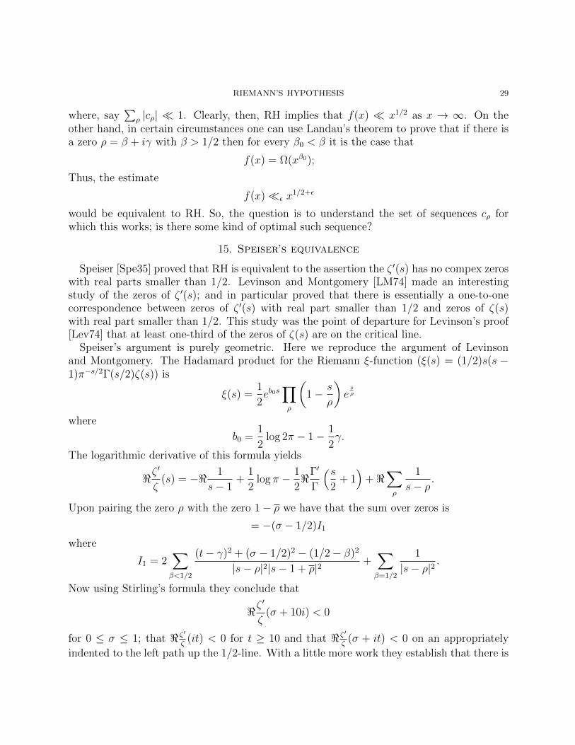
essentially a one-to-one correspondence between zeros of ζ(s) and zeros of ζ ′(s) to the rightof one-half; this is the subsequent starting point for Levinson’s proof that at least one-thirdof the zeros of ζ(s) are on the critical line σ = <s = 1/2. The figure below was made bySarah Froelich.
Figure 4. Zeros of ζ(s) in green and of ζ ′(s) in blue
16. Weil’s explicit formula and positivity criterion
Andre Weil [Wei52] (see also [Gui42]) proved the following formula which is a generalizationof Riemann’s formula mentioned above and which specifically illustrates the dependencebetween primes and zeros:
T (f) :=∑ρ
f(ρ) =
∫ ∞0
f(x) dx+
∫ ∞0
f ∗(x) dx−∞∑n=1
Λ(n)(f(n) + f ∗(n)
−(log 4π + γ)f(1)−∫ ∞
1
(f(x)− f ∗(x)− 2
xf(1)
)x dx
x2 − 1
holds whenever f ∈ C∞0 (0,∞) where f ∗(x) = 1xf(
1x
)and f(s) =
∫∞0f(x)xs−1 dx.
Using this Weil gave a criterion for RH. As stated by Bombieri [Bom00] it is as follows:The Riemann Hypothesis holds if and only if∑
ρ
g(ρ)g∗(1− ρ) > 0
for every complex-valued g(x) ∈ C∞0 (0,∞) which is not identically 0.
RIEMANN’S HYPOTHESIS 31
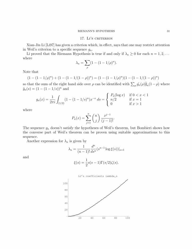
17. Li’s criterion
Xian-Jin Li [Li97] has given a criterion which, in effect, says that one may restrict attentionin Weil’s criterion to a specific sequence gn.
Li proved that the Riemann Hypothesis is true if and only if λn ≥ 0 for each n = 1, 2, . . .where
λn =∑ρ
(1− (1− 1/ρ)n).
Note that
(1− (1− 1/ρ)n) + (1− (1− 1/(1− ρ))n) = (1− (1− 1/ρ)n)(1− (1− 1/(1− ρ))n)
so that the sum of the right hand side over ρ can be identified with∑
ρ gn(ρ)gn(1− ρ) where
gn(s) = (1− (1− 1/s))n and
gn(x) =1
2πi
∫(1/2)
(1− (1− 1/s)n)x−s ds =
Pn(log x) if 0 < x < 1n/2 if x = 10 if x > 1
where
Pn(x) =n∑j=1
(n
j
)xj−1
(j − 1)!.
The sequence gn doesn’t satisfy the hypotheses of Weil’s theorem, but Bombieri shows howthe converse part of Weil’s theorem can be proven using suitable approximations to thissequence.
Another expression for λn is given by
λn =1
(n− 1)!
dn
dsn(sn−1 log ξ(s))|s=1
and
ξ(s) =1
2s(s− 1)Γ(s/2)ζ(s).
20 40 60 80 100
20
40
60
80
100
Li’s coefficients lambda_n
32 BRIAN CONREY
Bombieri and Lagarias [BL99] have pointed out that for any multiset R of complex num-
bers ρ for which 1 /∈ R and∑
ρ1+|<ρ|1+|ρ|2 is finite the following are equivalent:
• <ρ ≤ 1/2 for all ρ ∈ R;•∑
ρ<(1− (1− 1/ρ)−n) ≥ 0 for n = 0, 1, 2, . . . ;
• for every ε > 0 there is a c(ε) > 0 such that∑
ρ<(1 − (1 − 1/ρ)−n) ≥ −c(ε)eεn forn = 1, 2, 3, . . . .
Coffey [Cof05] has shown that
λn = S1(n) + S2(n) + 1− n
2(γ + log π + 2 log 2)
where
S1(n) :=n∑k=2
(−1)k(n
k
)(1− 2−k)ζ(k)
and
S2(n) := −n∑k=1
(n
k
)ηk−1
with
ηk :=(−1)k
k!limN→∞
( N∑m=1
Λ(m) logkm
m− logk+1N
k + 1
).
Regarding S1, he has proven that
S1(n) =1
2n log n− 1
2(1− γ)n+O(1);
regarding S2, he conjectures that
S2(n) n1/2+ε
which of course would imply RH.
18. Function field zeta-functions
See [Ros02] for an introduction to this subject. Let Fq be a field with q elements. Avariety over Fq has an associated zeta-function obtained by counting points on the varietyin extensions Fqn . The zeta-function has a functional equation and Euler product. Weilconjectured that the analogue of the Riemann Hypothesis holds for such zeta-functions.Deligne [Del74] proved Weil’s conjecture. This result stands today as a beacon for researcherstrying to understand the classical Riemann Hypothesis, but attempts to mimic the proof havegone awry. In the case that the variety is a curve Stepanov [Ste69] gave a proof different fromDeligne and in the spirit and flavor of work in transcendental number theory. See Bombieri’saccount [Bom74] of Stepanov’s method; also [IK04] gives a nice account of special cases ofthis proof.
RIEMANN’S HYPOTHESIS 33
A simple example of the kind of zeta-function we are talking about is as follows. For amonic polynomial f ∈ Fq[x] let N(f) = qdeg(f) where deg(f) is just the degree of f . We thinkof the monic polynomials f as being like the positive integers and form the zeta-function
Z(s) =∑
f monic
1
N(f)s.
This has an Euler product
Z(s) =∏
P irred.
(1− 1
N(P )s
)−1
where the product is over the monic irreducible polynomials P . It turns out that both thesum and the product are absolutely convergent for <s > 1. In fact, the number of monicpolynomials of degree d is precisely qd and so,
Z(s) =∞∑d=0
qd
qds=
1
1− q1−s .
There is a functional equation
1
1− qsZ(s) = Φ(s) = Φ(1− s).
In general, we can repeat the above situation, but with the integral domain Fq[x] replacedby Fq[x, y]/(g(x, y)) for some irreducible polynomial g. We have to define a notion of degreeso that we will have a multiplicative norm, but the same thing goes through and we have azeta-function and an Euler product. The general shape of the zeta-function is
H(1/qs)
1− q1−s
where H is a polynomial. There is a functional equation, which is the same thing as sayingthat the roots of the polynomial H(t) are invariant under t→ q/t. And there is a RiemannHypothesis, which is the assertion that all of the zeros of H(s) have real part equal to 1/2;equivalently, the roots of H(x) = 0 have absolute value q1/2.
Patterson, in his book [Pat88] on the zeta-function, gives examples of such “zeta-like”functions which have an Euler product and functional equation but do not satisfy the Rie-mann Hypothesis. His conclusion is that this indicates that a purely analytic proof of theRiemann Hypothesis is unlikely and that one needs to find some kind of an inner-productstructure that will give a positive pairing that will lead to the Riemann Hypothesis.
We want to counter that by observing that, in fact, the analogue of the Selberg axiomsfor this class of zeta-functions actually does imply the Riemann Hypothesis.
34 BRIAN CONREY
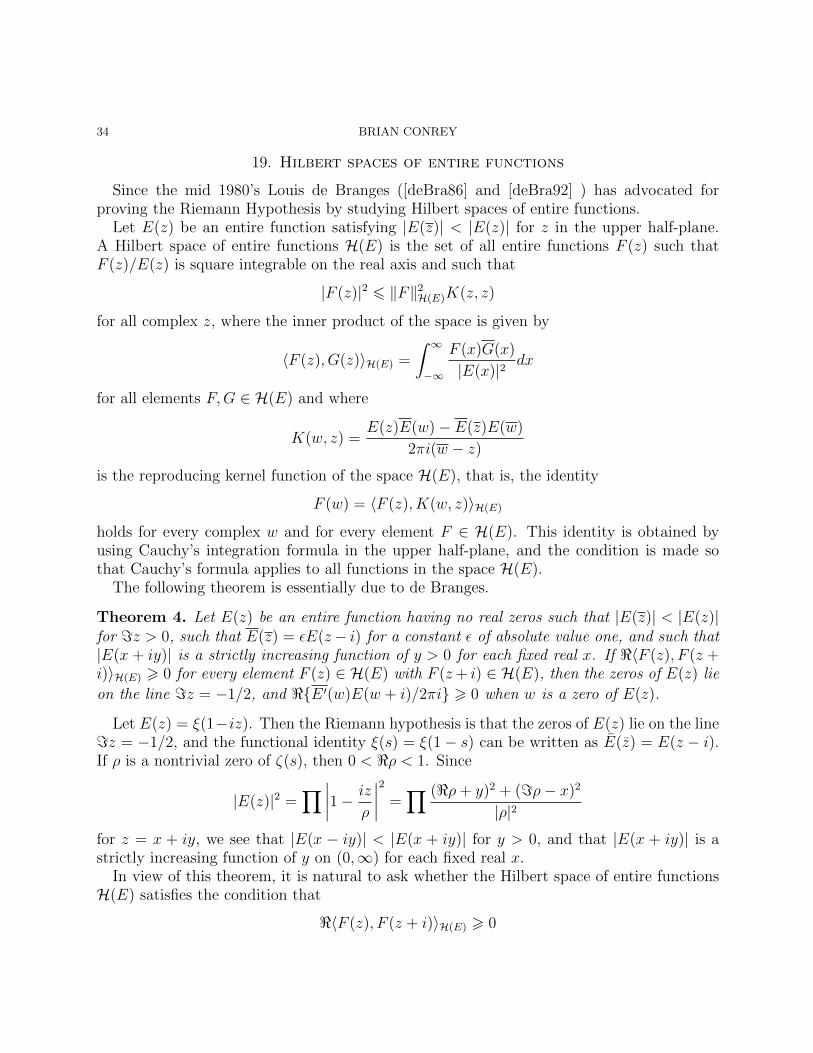
19. Hilbert spaces of entire functions
Since the mid 1980’s Louis de Branges ([deBra86] and [deBra92] ) has advocated forproving the Riemann Hypothesis by studying Hilbert spaces of entire functions.
Let E(z) be an entire function satisfying |E(z)| < |E(z)| for z in the upper half-plane.A Hilbert space of entire functions H(E) is the set of all entire functions F (z) such thatF (z)/E(z) is square integrable on the real axis and such that
|F (z)|2 6 ‖F‖2H(E)K(z, z)
for all complex z, where the inner product of the space is given by
〈F (z), G(z)〉H(E) =
∫ ∞−∞
F (x)G(x)
|E(x)|2dx
for all elements F,G ∈ H(E) and where
K(w, z) =E(z)E(w)− E(z)E(w)
2πi(w − z)
is the reproducing kernel function of the space H(E), that is, the identity
F (w) = 〈F (z), K(w, z)〉H(E)
holds for every complex w and for every element F ∈ H(E). This identity is obtained byusing Cauchy’s integration formula in the upper half-plane, and the condition is made sothat Cauchy’s formula applies to all functions in the space H(E).
The following theorem is essentially due to de Branges.
Theorem 4. Let E(z) be an entire function having no real zeros such that |E(z)| < |E(z)|for =z > 0, such that E(z) = εE(z− i) for a constant ε of absolute value one, and such that|E(x + iy)| is a strictly increasing function of y > 0 for each fixed real x. If <〈F (z), F (z +i)〉H(E) > 0 for every element F (z) ∈ H(E) with F (z+ i) ∈ H(E), then the zeros of E(z) lie
on the line =z = −1/2, and <E ′(w)E(w + i)/2πi > 0 when w is a zero of E(z).
Let E(z) = ξ(1−iz). Then the Riemann hypothesis is that the zeros of E(z) lie on the line=z = −1/2, and the functional identity ξ(s) = ξ(1− s) can be written as E(z) = E(z − i).If ρ is a nontrivial zero of ζ(s), then 0 < <ρ < 1. Since
|E(z)|2 =∏∣∣∣∣1− iz
ρ
∣∣∣∣2 =∏ (<ρ+ y)2 + (=ρ− x)2
|ρ|2
for z = x + iy, we see that |E(x − iy)| < |E(x + iy)| for y > 0, and that |E(x + iy)| is astrictly increasing function of y on (0,∞) for each fixed real x.
In view of this theorem, it is natural to ask whether the Hilbert space of entire functionsH(E) satisfies the condition that
<〈F (z), F (z + i)〉H(E) > 0
RIEMANN’S HYPOTHESIS 35
for every element F (z) of H(E) such that F (z + i) ∈ H(E), because the nontrivial zerosof the Riemann zeta function ζ(s) would then lie on the critical line <s = 1/2 under thiscondition. However, this is not true as the following example shows.
Let ρ = 1/2 + i111.0295355431696745 · · · be the 34th zero of the Riemann zeta functionin the upper half-plane. By using MATHEMATICA, we compute that
−<ξ′(ρ)ξ(1 + ρ) = −5.389100507182945 · · · × 10−69 < 0.
Write ρ = 1− iw. Then E(w) = 0, and E ′(w)E(w + i)/i = −ξ′(ρ)ξ(1 + ρ). Thus, we have
<E ′(w)E(w + i)/2πi < 0.
The conclusion is that E(z) = ξ(1− iz) is not a structure function of a de Branges space.Lagarias [Lag06] has written an account of some of these investigations. He has shown
that
Theorem 5. Let
Eζ(z) = ξ(1/2− iz) + ξ′(1/2− iz).
Then Eζ(z) is the structure function of a de Branges space H(Eζ(z)) if and only if theRiemann Hypothesis is true.
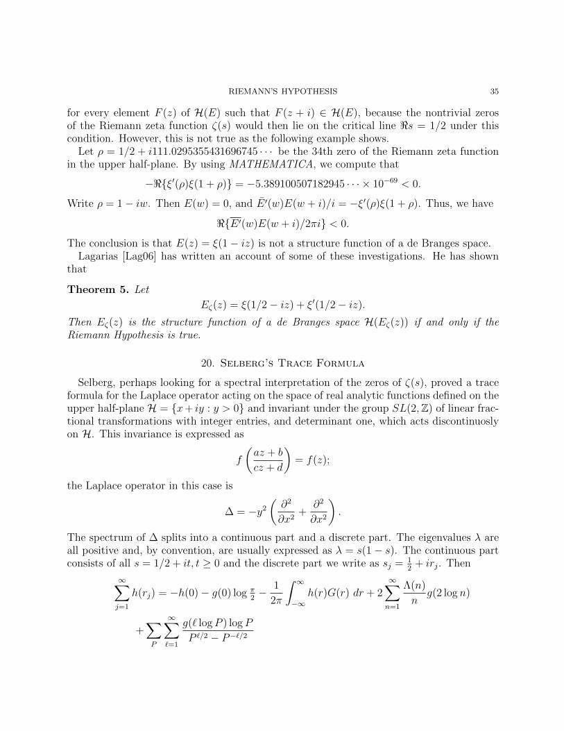
20. Selberg’s Trace Formula
Selberg, perhaps looking for a spectral interpretation of the zeros of ζ(s), proved a traceformula for the Laplace operator acting on the space of real analytic functions defined on theupper half-plane H = x+ iy : y > 0 and invariant under the group SL(2,Z) of linear frac-tional transformations with integer entries, and determinant one, which acts discontinuoslyon H. This invariance is expressed as
f
(az + b
cz + d
)= f(z);
the Laplace operator in this case is
∆ = −y2
(∂2
∂x2+
∂2
∂x2
).
The spectrum of ∆ splits into a continuous part and a discrete part. The eigenvalues λ areall positive and, by convention, are usually expressed as λ = s(1− s). The continuous partconsists of all s = 1/2 + it, t ≥ 0 and the discrete part we write as sj = 1
2+ irj. Then
∞∑j=1
h(rj) = −h(0)− g(0) log π2− 1
2π
∫ ∞−∞
h(r)G(r) dr + 2∞∑n=1
Λ(n)
ng(2 log n)
+∑P
∞∑`=1
g(` logP ) logP
P `/2 − P−`/2
36 BRIAN CONREY
where g and h are as in Weil’s formula and
G(r) =Γ′
Γ(1
2+ ir) +
Γ′
Γ(1 + ir)− π
6r tanhπr +
π
coshπr(1
8+√
39
cosh πr3
).
Also, the sum is over the norms P of prime geodesics of Γ\H. The values taken on by Pare of the form (n +
√n2 − 4)2/4 with n ≥ 3 with certain multiplicities (the class number
h(n2−4)). H. Haas was one of the first people to compute the eigenvalues r1 = 9.533 . . . , r2 =12.173 . . . , r3 = 13.779 . . . of SL2(Z) in 1977 in his University of Heidelberg Diplomarbeit.Soon after, Hejhal was visiting San Diego, and Audrey Terras pointed out to him thatHaas’ list contained the numbers 14.134 . . . , 21.022 . . . ; the ordinates of the first few zerosof ζ(s) were lurking amongst the eigenvalues! Hejhal discovered the ordinates of the zerosof L(s, χ3) (see section 7) on the list, too. He unraveled this perplexing mystery about 6months later. It turned out that the spurious eigenvalues were associated to “pseudo cuspforms” and appeared because of the method of computation used. If the zeros had appearedlegitimately, RH would have followed because λ = ρ(1 − ρ) is positive. (The 1979 IHESpreprint by P. Cartier and D. Hejhal contains additional details.)
The trace formula resembles the explicit formula in certain ways. Many researchers haveattempted to interpret Weil’s explict formula in terms of Selberg’s trace formula.
21. A trace formula in noncommutative geometry
Alain Connes’ approach (see [Conn99]) is to construct a space and an operator for whichthe zeros of the Riemann zeta-function on the critical line are the eigenvalues. Then analysisvia the explicit formula of Weil would analyze the trace of this operator and reveal that infact all of the zeros are in the spectrum.
As a naive example:
We know RH is equivalent to∑ρ
1
|ρ|2=∑ρ
1
ρ(1− ρ)= 2 + γ − log 4π.
So, we try to evaluate∑
1/|ρ(1 − ρ)| by using Weil’s explicit formula. (Thetest function in Weil does not have to be analytic.) We do an adelic versionof Weil and pay particular attention to what happens at all of the primes. Inthe end we end up with a formula for our sum. If it is equal to the answer weknew from the start them we have proven RH!
In Connes’ construction the space was a Hilbert space and eigenvalues were the zerosof ζ(s) on the line. Ralf Meyer has amended the construction to give an operator on aspace of rapidly decaying functions in which the eigenvalues are all of the zeros of ζ(s); thusthe explicit formula appears as a trace formula. However, it is not clear how to prove thepositivity. See [Conn99] and [Mey04] for more details.
See also [Wat02], and [Lac04] for explicit descriptions of Connes’ approach.
RIEMANN’S HYPOTHESIS 37
22. Dynamical systems approaches
In dynamical systems one begins with a classical Hamiltonian H(x, p) where x is positionand p is momentum and H is the total energy of the system. Hamilton’s equations are dx
dt= ∂H
∂pdpdt
= −∂H∂x
In the quantized dynamical system one has the Schrodinger equation
Hψ = Eψ.
Here ψ is a wave function and H is an operator, the quantum Hamilton, which is obtainedfrom H by replacing p with − i∂
∂x. For example if
H(x, p) =x2
2m+ V (x)
then
H =1
2m
∂2
∂x2+ V (x)
and the Schrodinger equation is
1
2mψ′′(x) + V (x)ψ(x) = Eψ(x).
Here E is a constant, energy. One wants to know about the eigenvalues of this equation.The challenge is to construct such a system in which the eigenvalues are the zeros of Ξ(t).In one dimension on a finite interval the eigenvalues are well-spaced; this is the situation ofSturm-Liouville operators for which many of the special functions of classical physics haveall of their zeros well-spaced on a line. In particular this situation cannot give the rightdensity of zeros. In two dimensions, one does conjecturally get Random Matrix statistics (egquantum billiards) but here we have way too many eigenvalues.
Berry and Keating [BK99], see also [BK11], have looked at the dynamical system xp onthe positive real line (i.e. not compact). Here one has
H(x, p) =1
2xp+
1
2px
and
H =−i2x∂
∂x− −i
2
∂
∂xx
and the Shrodinger equation is
−i(
1
2+ x
∂
∂x
)ψ = Eψ.
This has all of it’s eigenvalues on the 1/2-line and eigenfunctions
ψ(x) =1
x1/2+IE
38 BRIAN CONREY
With the boundary condition∞∑n=1
ψ(nx) = 0
one would then might expect the eigenvalues to be the zeros of ζ(s). However the operatoris not self-adjoint with respect to this boundary condition.
23. The Lee-Yang theorem
Although not directly connected to the Riemann Hypothesis, the Lee-Yang theorem [LY52]is of considerable interest in the study of zeros. Basically it says that the zeros of the partitionfunction of a ferromagnetic Ising model are all on the unit circle.
Mark Kac in his comment on Polya’s Bemerkung uber die Intergaldarstellung der Rie-mannschen ξ-Funktion [Pol26] writes
Although this beautiful paper takes one to within a hair’s breadth of Rie-mann’s Hypothesis it does not seem to have inspired much further work andreferences to it in the subsequent mathematical literature are rather scant.
Because of this it may be of interest to related that the paper did playa small, but perhaps not wholly negligible, part in the development of aninteresting and important chapter in Statistical Mechanics.
In the fall of 1951 and the spring of 1952 C. N. Yang and T. D. Lee weredeveloping their theory of phase transitions which has since become justlycelebrated. To illustrate their theory they introduced the concept of a “latticegas” and they were led to a remarkable conjecture which (not quite in its mostgeneral form) can be stated as follows:
Let
GN(z) =∑
exp
(N∑
k,`=1
Jk,`µkµ`
)exp(iz
N∑k=1
µk)
where Jk,` ≥ 0 and the summation is over all 2N sequences µ1, µ2, . . . , µN witheach µk assuming only values pm1.
Then GN(z) has only real zeros.When I first heard of this conjecture I tried the simplest case
Jk,` = ν/2
for all k and ` and somehow Hilfsatz II of Polya’s paper came to mind.
Kac goes on to describe how one can prove this special case via a slight modification ofPolya’s proof. Kac showed the proof to Yang and Lee and within a coule of weeks they hadproduced the proof of their general theorem [LY52].
A question now is: Is ζ(s) the partition function of some spin system?

RIEMANN’S HYPOTHESIS 39
24. Newman’s conjecture
Newman found a very general form of the Lee-Yang theorem, see [New76].In subsequent work he found an interesting approach to RH.It is known that Φ(u) decays very rapidly. In fact, doubly exponentially:
Φ(u) e9|u|/2e−πe2|u|.
Thus,
H(λ, z) :=
∫ ∞−∞
Φ(u)eλu2
eizu du
is rapidly convergent for any real λ. Also, H(0, z) = Ξ(z). It follows from a theorem ofdeBruijn that if for some λ0 all of the zeros of H(λ0, z) are real, then the same is true ofH(λ, z) whenever λ > λ0. Newman [New91] proved that there does exist such a λ0 and thatλ0 ≥ 1/8. He also proved that there exists a λ1 such that H(λ1, z) has a non-real zero. Thus,λ0 is bounded below. RH is the assertion that λ0 ≤ 0. Newman conjectures that λ0 = 0.Odlyzko has shown that H(−2.7× 10⁻⁹, z) has a non-real zero. Therefore, as Newman says,“. . . the Riemann hypothesis, if true, is only barely so.”
25. Stable polynomials
The remarkable work of Branden and Borcea, see [BB09], [BB09b], and [BB09c], aboutthe generalization to several variables of their solution of the Polya-Schur conjecture is worthnoting, especially since it has just played an important role in the solution of the Kadison-Singer problem by Marcus, Spielman, and Srivastava [MSS14].
We briefly describe their results. First of all a polynomial f in z1, . . . , zn is stable iff(z1, . . . , zn) 6= 0 for any n-tuple with all =zj > 0. If the coefficients are real then f is calledreal stable. Real stable polynomials in one variable have only real zeros.
Branden and Borcea characterize real stable polynomials in two variables as those express-ible as
f(z, w) = ± det(zA+ wB + C)
where A and B are positive definite and C is symmetric.In his 1988 Gibbs lecture [Rue88] David Ruelle proclaimed about the Lee-Yang theorem:
“I have called this beautiful result a failure because, while it has important applications inphysics, it remains at this time isolated in mathematics. One might think of a connectionwith zeta-functions (and the Weil conjectures); the idea of such a connection is not absurd,as our second example will show. But the miracle has not happened: one still does not knowwhat to do with the circle theorem.”

40 BRIAN CONREY
Lieb and Sokal [LS81] reduced the generalized Lee-Yang theorem to the assertion: ifP,Q ∈ C[z1, . . . , zn] are non-vanishing when all of the variables are in the open right half-plane then the polynomial
P
(∂
∂z1
, . . . ,∂
∂zn
)Q(z1, . . . , zn)
also has this property. Thus, to better understand Lee-Yang-type theorems one is naturallyled to consider the problems of describing linear operators on polynomial spaces that preservethe property of being nonvanishing when the variables are in prescribed subsets of Cn.
26. Nyman – Beurling approach
This approach begins with the theorem of Nyman [Nym50], a student of Beurling. Thework of Beurling and Nyman [Beu55] implies that RH can be recast as an approximationproblem in a certain Hilbert space. Let x denote the fractional part of x. One considersfunctions of the form
f(x) =n∑k=1
ckθk/x
where 0 < θk ≤ 1 and ck are complex numbers and asks whether the characteristic functionχ(x) = χ(0,1](x) can be approximated by such f on the positive real line. Their theorem isthat the Riemann Hypothesis holds if and only if
limn→∞
infck,θk
∫ ∞0
|χ(x)−n∑k=1
ckθk/x|2 dx = 0
This theorem has been extended by Baez-Duarte, [B-D02] and [B-D03b], who showed thatone may take θk = 1/k. So, let
dn := infc1,...,cn
∫ ∞0
|χ(x)−n∑k=1
ck1/(kx)|2 dx.
Thus, the Riemann Hypothesis holds if and only if limn→∞ dn = 0.It is conjectured that dn ∼ C
lognwhere C =
∑ρ
1|ρ|2 . Burnol [Bur03] has proven that
1
log n
∑ρ on the line
mρ
|ρ|2
is a lower bound. If RH holds and all the zeros are simple, then clearly these two boundsare the same.
Note that it is easy to see that∑ρ
1
ρ(1− ρ)= 2 + γ − log 4π = 0.04619 . . .
RIEMANN’S HYPOTHESIS 41
Just begin with
I =1
2πi
∫(2)
ζ ′
ζ(s)
ds
s(1− s).
On the one hand, this integral is 0 as can be seen by moving the path arbitrarily far to theright; on the other hand the integral can be evaluated by moving the path arbitrarily far tothe left and accounting for residues of poles at s = 1, 0, ρ,−2n. In this way we get the result.
An easy exercise shows that the Riemann Hypothesis is equivalent to∑ρ
1
|ρ|2= 2 + γ − log 4π.
A rephrasing of the Baez-Duarte theorem (by Balazard and Saias, see [BS98], [BS00], and[BS04]) arises from taking the Mellin transform of f . In this way one finds that the RiemannHypothesis holds if and only if
limN→∞
infAN
∫ ∞−∞|1− AN(1/2 + it)ζ(1/2 + it)|2 dt
14
+ t2= 0
where the infimum is over all Dirichlet polynomials AN(s) =∑N
h=1ahhs
of length N . Now theproblem looks like a mollification problem.
Bagchi [Bag06] has written a very nice exposition explaining this complicated circle ofideas.
26.1. The Vasyunin sums. Consider
IN(~a) =
∫ ∞−∞|1− AN(1/2 + it)ζ(1/2 + it)|2 dt
14
+ t2.
Let’s assume for convenience that the coefficients ah are real. Squaring out, we have
IN(~a) =
∫ ∞−∞
dt14
+ t2− 2
i
∫(1/2)
ζ(s)AN(s)ds
s(1− s)+
∫ ∞−∞|ζAN(1/2 + it)|2 dt
14
+ t2
= 2π + 4π((1− γ)AN(1)− A′N(1)) + 2πN∑
h,k=1
ahakbh,k
where
bh,k =1√hk
∫ ∞−∞|ζ(1/2 + it)|2 (h/k)it
14
+ t2dt.
Writing this as a complex integral, we see that
bh,k2π
=1
2πi
∫(1/2)
ζ(s)
shsζ(1− s)
(1− s)k1−s ds.
42 BRIAN CONREY
We recognize this as a convolution of Mellin transforms, and calculate that
1
2πi
∫(1/2)
ζ(s)
shsu−s ds = − 1
uh+∞∑n=1
1
2πi
∫(1/2)
(nhu)−s
sds
= − 1
uh+∑nuh≤1
1 = −
1
uh
if 1/(uh) is not an integer; if it is, subtract 1/2. Thus, using the formula for convolution, wefind that
bh,k2π
=
∫ ∞0
1
hx
1
kx
dx.
Remarkably, Vasyunin [Vas95] found a beautiful exact formula for the right side here. Note,first of all, that
bh,k =bH,K(h, k)
where h = (h, k)H and k = (h, k)K. Thus, it suffices to evaluate bh,k when (h, k) = 1. So,assuming that h and k are relatively prime, and letting
V (h, k) :=k−1∑a=1
ah
k
cot
πa
k,
then Vasyunin’s formula implies that
bh,k2π
=log 2π − γ
2
(1
h+
1
k
)+k − h2hk
logh
k− π
2hk(V (h, k) + V (k, h)) .
The following estimate is easy to prove:
c0(1, k) =k
π
(log
k
2π+ γ
)+
1
π+O(1/k).
More challenging is the reciprocity formula, see [BC13] and [BC13b],
Theorem 6. There exists a function g(z) analytic on C† which is the complex plane withthe negative real axis removed such that for any k > 0 and (h, k) = 1,
h
kc0(h, k) + c0(k, h)− 1
πk= g(h/k).
One would hope that this formula could be useful in analyzing dn.As mentioned earlier it is believed that
d2n ∼
2 + γ − log 4π
log n
as n→∞. In [BCF12] the following is proven.
RIEMANN’S HYPOTHESIS 43
Theorem 7. Let
VN(s) =∑n≤N
µ(n)log N
n
logN
ns.
If the Riemann hypothesis is true and if∑|=(ρ)|≤T
1
|ζ ′(ρ)|2 T
32−δ
for some δ > 0, then
1
2π
∫ ∞−∞|1− ζVN(1/2 + it)|2 dt
14
+ t2∼ 2 + γ − log 4π
logN.
The condition implicitly assumes that the zeros of the Riemann zeta function are allsimple. Moreover, this upper bound is “mild” in the sense that a conjecture, due to Gonekand recovered by a different heuristic method of Hughes, Keating, and O’Connell [HKO00],predicts that ∑
|ρ|≤T
1
|ζ ′(ρ)|2∼ 6
π3T.
Thus, VN gives an asymptotically optimal choice.
27. Eigenvalues of Redheffer’s matrix
The Redheffer matrix A(n) is an n×n matrix of 0’s and 1’s defined by A(i, j) = 1 if j = 1or if i divides j, and A(i, j) = 0 otherwise. It has the property that
detA(n) = M(n)
the summatory function of the Mobius function. Thus, RH is true if and only detA(n) n1/2+ε and so it is of interest to study the eigenvalues; see [BFP89].
It is known that A(n) has n−[log n/ log 2]−1 eigenvalues equal to 1. One way to see this isto interpret the matrix minus the identity as the incidence matrix of a graph. The coefficientsof the characteristic polynomial are easily described by counting “cycles” of divisors: suchas 1→ 2→ 4→ 12→ 60 would be a cycle of length 5 that occurs in any graph with n ≥ 60.Letting Sk(n) be the number of such cycles of length k in the graph with n vertices, thedesired characteristic polynomial, but with all of the eigenvalues equal to 1 removed, is ofdegree N = [log n/ log 2] + 1 and is given by
Pn(λ) = (λ− 1)N −N−1∑k=1
Sk(n)(λ− 1)N−1−k
Another way to think of this is to let Dk(m) be the number of ways to factor m into aproduct of k integers each greater than 1, taking order into account. So, Dk(m) is like dk(m)
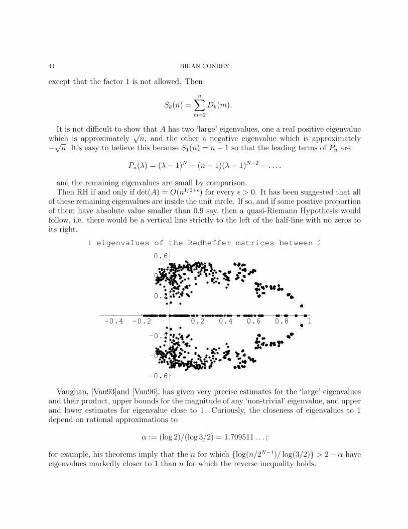
44 BRIAN CONREY
except that the factor 1 is not allowed. Then
Sk(n) =n∑
m=2
Dk(m).
It is not difficult to show that A has two ‘large’ eigenvalues, one a real positive eigenvaluewhich is approximately
√n, and the other a negative eigenvalue which is approximately
−√n. It’s easy to believe this because S1(n) = n− 1 so that the leading terms of Pn are
Pn(λ) = (λ− 1)N − (n− 1)(λ− 1)N−2 − . . . .
and the remaining eigenvalues are small by comparison.Then RH if and only if det(A) = O(n1/2+ε) for every ε > 0. It has been suggested that all
of these remaining eigenvalues are inside the unit circle. If so, and if some positive proportionof them have absolute value smaller than 0.9 say, then a quasi-Riemann Hypothesis wouldfollow, i.e. there would be a vertical line strictly to the left of the half-line with no zeros toits right.
-0.4 -0.2 0.2 0.4 0.6 0.8 1
-0.6
-0.4
-0.2
0.2
0.4
0.6
trivial eigenvalues of the Redheffer matrices between 200
Vaughan, [Vau93]and [Vau96], has given very precise estimates for the ‘large’ eigenvaluesand their product, upper bounds for the magnitude of any ‘non-trivial’ eigenvalue, and upperand lower estimates for eigenvalue close to 1. Curiously, the closeness of eigenvalues to 1depend on rational approximations to
α := (log 2)/(log 3/2) = 1.709511 . . . ;
for example, his theorems imply that the n for which log(n/2N−1)/ log(3/2) > 2− α haveeigenvalues markedly closer to 1 than n for which the reverse inequality holds.
RIEMANN’S HYPOTHESIS 45
Here is a slightly different approach which is implicit in Vaughan’s work.
∞∑n=1
µ(n)
ns=
1
ζ(s)=
1
1 + (ζ(s)− 1)=∞∑k=0
(−1)k(ζ(s)− 1)k =∞∑k=0
(−1)k∞∑n=1
Dk(n)
ns
so that
µ(n) =∞∑k=0
(−1)kDk(n)
and
M(n) =n∑
m=1
µ(m) =∞∑k=0
(−1)kSk(n).
Now, if we perturb this argument (due to Vaughan) slightly we can nearly recover Redehef-fer’s characteristic polynomial. Let
∞∑m=1
µw(m)
ms:=
1
1 + w(ζ(s)− 1)=∞∑k=0
(−1)kwk(ζ(s)− 1)k =∞∑k=0
(−1)kwk∞∑m=1
Dk(m)
ms
so that
µw(m) =∞∑k=0
(−1)kwkDk(m)
and, after summing m from 1 to n, we have
Mw(n) :=n∑
m=1
µw(m) =∞∑k=0
(−1)kwkSk(n) =N∑k=0
(−1)kwkSk(n).
Then
(1− λ)−NM1−λ(n) ≈ Pn(λ).

46 BRIAN CONREY
-0.5 -0.25 0.25 0.5 0.75 1 1.25 1.5
-1
-0.75
-0.5
-0.25
0.25
0.5
0.75
1-trivial reciprocal zeros of M_wHnL for 200 < n <
28. Bombieri’s Theorem
Bombieri [Bom00] has proven that one of the following assertions is true:
• The Riemann Hypothesis• There are infinitely many zeros of ζ(s) to the right of the critical line.• There are coefficients cρ such that
∑ρ |cρ|2 = 1 and
∑<ρ6=1/2 |cρ|2 ≥ 1/2 for which
the linear combination∑ρ
cρρ(1− ρ)
x−ρ + A+B/x
for some constants A and B vanishes identically in some interval 1 ≤ x ≤M0 whereM0 > 1 is an explicitly computable constant.
The idea is to rule out the third possibility here so that one can say that if RH is false, theninfinitely many zeros are off the line. If one had a quantitative version of such an assertion,it might contradict, for example, the density estimate for N(σ, T ) cited above.
Bombieri’s analysis is interesting. He begins with Weil’s criterion but applied to a Hilbertspace of functions supported on a finite closed interval [M−1,M ]. He looks for functions gfor which ||g|| = 1 and
∑ρ g(ρ)g(1− ρ) is minimal. The inner product on the Hilbert space
is defined by
〈f, g〉 =
∫ M
M−1
f(x)g(x) dx.
RIEMANN’S HYPOTHESIS 47
Using Weil’s explicit formula he finds a convenient expression for the Euler-Lagrange equa-tion. He can essentially solve this as a linear combination as mentioned here.
Here are some further details. Let T (f) be as in Weil’s explicit formula. Let ta[f ] be thefunction defined by ta[f ](x) = f(ax). Let L[f ] be the function defined at a number x byL[f ](x) = T (tx[f ]). The convolution of f and g, denoted by f ∗ g is defined, as usual, to bethe function whose value at x is
(f ∗ g)(x) =
∫ ∞0
f(u)g(x/u)du
u.
Recall that f ∗(x) = f(1/x)/x. Observe that
(f ∗ g∗)(x) =
∫ ∞0
f(ux)g(u) du = 〈tx[f ], g〉.
To prove RH we have to show that
T (f ∗ f ∗) > 0
for all suitable f .The idea is to use the calculus of variations to find the minimal f , say on the interval
(M−1,M) subject to something like 〈f, f〉 = 1. So, suppose that f is a minimal functionand consider f + εφ where φ(M−1) = φ(M) = 0. Then, d
dεI(f + εφ)
∣∣ε=0
= 0 where
I(f) =T (f ∗ f ∗)〈f, f〉
.
We have
0 =d
dεΦ(f + εφ) =
〈f, f〉 ddεT ((f + εφ) ∗ (f ∗ + εφ∗))− T (f ∗ f ∗) d
dε〈f + εφ, f + εφ〉
〈f, f〉2
so that
〈f, f〉T (f ∗ φ∗) = T (f ∗ f ∗)〈f, φ〉
for all φ. Now
T ((f ∗ φ∗)(x)) = T (〈tx[f ], φ〉) = 〈T (tx[f ]), φ〉 = 〈L[f ](x), φ〉.
Thus, the above becomes
〈L[f ]− λf, φ〉 = 0
for all suitable φ where
λ =T (f ∗ f ∗)〈f, f〉
.
We conclude that a minimal such f must satisfy L[f ] = λf , i.e.
〈f, f〉L[f ] = T (f ∗ f ∗)f.

48 BRIAN CONREY
Recall that Weil’s explicit formula says that
T (f) =∑ρ
f(ρ).
Thus,
L[f ](x) = T (tx[f ]) =∑ρ
˜tx[f ](ρ) =∑ρ
f(ρ)x−ρ
so that ∑ρ
f(ρ)x−ρ = λf(x).
Now let φ(x) be the characteristic function of the interval [M−1,M ] and consider functionsf given by
f(x) =∑ρ
Xρφ(x)x−ρ.
Then
f(s) =∑ρ
Xρφ(s− ρ).
So, if Xρ = f(ρ)/λ, then f is formally a solution. This leads to the eigenvalue problem
λXρ =∑ρ′
φ(ρ− ρ′)Xρ′ .
We calculate that
φ(s) =
∫ M
M−1
xsdx
x=M s −M−s
s.
Now we introduce some new notation. Let ρ = 1/2 + iγ (with γ ∈ C); M = et with t > 0;Λ = 1/λ; zγ = Xρ; wγ =
(14
+ γ2)zγ; K(x) = sinx
xand
H(x, y, t) =2tK(t(x− y))
14
+ y2.
Then the eigenvalue problem can be rewritten as
wγ = Λ∑γ′
H(γ, γ′, t)wγ′ .
Next, let
H(Γ, t) =[H(γ, γ′, t)
]γ,γ′∈Γ
and the resolvent determinant
D(Λ, t) = detH(I − ΛΓ; t).

RIEMANN’S HYPOTHESIS 49
Bombieri proves that D(Λ, t) is an entire function in Λ of order at most 1, and that
D(Λ, t) = 1 +∞∑n=1
(−1)n∆n(t)Λn
n!
where
∆n(t) =∑
γ1,...,γn∈Γ
det[H(γj, γk, t)
]j,k=1,...,n
.
Moreover, the truncations
DN(Λ, t) = det[δγ,γ′ − ΛH(γ, γ′, t)
]∣∣γ,γ′∈ΓN
,
where ΓN is the set of γ ∈ Γ with |γ| ≤ N , converge to D(Λ, t) uniformly on compact sets,as N →∞.
The zeros of the resolvent give the solutions to our linear system. Let Λ0 be a zero ofD(Λ, t) and define
D(γ, γ0; Λ, t) = Λ∞∑n=0
(−1)n∆n(γ, γ0; t)Λn
n!
where ∆0(γ, γ0; t) = H(γ, γ), t) and
∆n(γ, γ0; t) =∑
γ1,...,γn∈Γ
det
[H(γ, γ0, t) H(γ, γk, t)H(γj, γ0, t) H(γj, γk, t)
]j,k=1,...,n
Then D(γ, γ0; Λ, t) is an entire function of Λ of order at most 1, and there exists a γ0 suchthat
wγ = D(γ, γ0; Λ0, t)
is a solution, not identically 0, to the system above. Moreover,
f(x) =∑ρ
Xρφ(x)x−ρ
with Xρ = wγ and M = et satisfies
f(x) = Λ0L[f ](x) x ∈ (1/M,M)
and f(1/M) = f(M) = 0.So, we (i.e. Bombieri) have “constructed” an extremal function for Weil’s “quadratic
functional.”The next step is to investigate finite approximations to this problem. In other words,
consider what the situation is for finite sets Λ. Bombieri considers a general situation wherethe numbers in Γ are arbitrary but have the same symmetries as do zeta-zeros. He showsthat all of the eigenvalues Λ are real, and that if all of the γ ∈ Γ are real then all of theeigenvalues Λ are positive. In fact, the number of non-real pairs of conjugate γ is exactlyequal to the number of negative eigenvalues.

50 BRIAN CONREY
29. The Selberg Class of Dirichlet series
Selberg [Sel89] has introduced a class of Dirichlet series and made certain conjecturesabout them. We let S denote the class of functions in question. A Dirichlet series
F (s) =∑ a(n)
ns
is in S provided that it satisfies the following hypotheses:
• Analyticity: (s− 1)mF (s) is an entire function of finite order for some non-negativeinteger m• Ramanujan Hypothesis: an nε for any fixed ε > 0• Functional equation: there must be a function γF (s) of the form
γF (s) = εQs
k∏i=1
Γ(λis+ µi)
where |ε| = 1, Q > 0, λi > 0, and <µi ≥ 0 such that
Φ(s) = γF (s)F (s)
satisfiesΦ(s) = Φ(1− s)
• Euler product: a1 = 1, and
logF (s) =∑ bn
ns
where bn = 0 unless n is a positive power of a prime and bn nθ for some θ < 1/2.
Selberg conjectures that any Dirichlet series in the Selberg class satisfies a Riemann Hy-pothesis, that all of its non-trivial zeros have real part equal to 1/2.
Here are two examples of functions in the Selberg class:
L4(s) = 1− 1
3s+
1
5s− 1
7s+ · · · =
∏p≥3
(1− χ−4(p)
ps
)−1
satisfies the functional equation(4
π
)s/2Γ
(s
2+
1
2
)L4(s) = ξ4(s) = ξ4(1− s);
and, letting x∏∞
n=1(1− xn)24 =∑∞
n=1 τ(n)xn define Ramanujan’s tau-function,
Lτ (s) =∞∑n=1
τ(n)/n11/2
ns=∏p
(1− τ(p)/p11/2
ps+
1
p2s
)−1
satisfies
(2π)−sΓ(s+ 11/2)Lτ (s) = ξτ (s).
RIEMANN’S HYPOTHESIS 51
One needs Mordell’s theorem τ(m)τ(n) =∑
d|n d11τ(mn/d2) and Deligne’s theorem |τ(p)| ≤
2p11/2, both conjectured by Ramanujan, to verify that Lτ ∈ S.
30. Real zeros of quadratic L-functions
A collection of problems which may be relevant to solving RH is as follows. Let Lp(s) =∑χp(n)n−s where χp(n) =
(np
)is the Legendre symbol which is equal to 0 if n is a multiple
of p and otherwise is 1 if n is a square mod p and −1 if n is not a square modulo the primenumber p. The series for Lp(s) converges if <s > 0. The problem is to prove that Lp(σ) > 0for 0 < σ < 1.
Depending on your point of view, this may seem like an easier problem than RH or aharder one. But I believe that it is exactly the same difficulty. It is certainly easier to statethan RH! The reason I like this problem is that it removes the temptation to use analysis toprove RH. On the surface RH looks like a problem in analysis, and so analysts try all sortsof tricks. However, if one believes that the problem is essentially number theoretic, then thisversion puts one on more realistic turf. Also, perhaps the real difficulty with proving RHcomes into view. That is that the Dirichlet series
Λ(s) =∞∑n=1
λ(n)
ns
really does have a zero at s = 1! It has an Euler product, as does Lp(s). It also has afunctional equation, though of a slightly different character, in that the Gamma-functionappears in the denominator rather than the numerator of the factor relating this function ats and at 1 − s. Moreover, can find primes p such that the two Dirichlet series agree for anarbitrarily long initial stretch. Thus, there is a tendency for certain p for Lp(s) to want tohave a zero at, or near s = 1. It is this tension that, I believe, causes the intrinsic difficultywith proving RH. Somehow, one has to understand and explain the essential differencebetween these two objects.
Of course, a significant difference is that the χp(n) are periodic functions of n (with periodp) whereas λ(n) is not. This leads to the deduction that the Lp(s) are entire functions,whereas Λ(s) is not entire. But how can one make use of this fact?
One attempt actually does take us back into analysis. That is through the representation
Γ(s)Lp(s) =
∫ ∞0
e−xxsdx
x
∞∑n=1
χp(n)
ns=
∫ ∞0
∞∑n=1
χp(n)e−nxxsdx
x
=
∫ ∞0
p−1∑n=1
χp(n)e−nx
1− e−pxdx
x=
∫ ∞0
Fp(e−x)
dx
(1− e−px)x
=
∫ 1
0
Fp(u) du
(1− up)u log 1u
52 BRIAN CONREY
where
Fp(u) =
p−1∑n=1
χp(n)un
is the Fekete polynomial. Note that if Fp(u) > 0 for 0 < u < 1 then it follows thatLp(σ) > 0 for 0 < σ < 1. For small p this idea works reasonably well. For example, F5(u) =u−u2−u3 +u4 > 0. In fact, of the primes up to 100, only 43 and 67 have Fekete polynomialsthat have zeros in [0, 1]. However, if χp(2) = χp(3) = χp(5) = χp(7) = χp(11) = −1 thenFp(0.7) < 0 as shown by Polya. In fact, it is not known whether Fp(σ) > 0 for all 0 < σ < 1and infinitely many p. On the other hand, it has been shown by Conrey and Soundararajan[CS02] that for infinitely many p, (in fact, a positive proportion of p) the inequality Lp(σ) > 0holds for all σ > 0. Watkins [W] has shown that these L-functions with odd characters donot vanish for p < 3× 10⁸.
In the spirit of this section we present the following inequality which implies RH.Let q > 0 be squarefree with q ≡ 3 mod 4 and let h(q) be the class number of the
imaginary quadratic field K = Q(√−q). Let χq be the Jacobi symbol modulo q so that χq
is the quadratic character associated with K. Suppose that
Sq(N) :=N∑n=1
χq(n)(1− n
N
)6 h(q) = Sq(q/2)
for all q as described above and all N < q4. Then all complex zeros of the Riemann zeta-
function have real part equal to 1/2.This inequality has been checked for q < 5000.
31. An orthogonal family
The book of Iwaniec and Kowalski [IK04], Section 3.8, is a good reference for the materialin this section, as is [GZ80], from which much of this material is taken. See also [RVZ93]and [CSn13]. Let
η =1 +√−7
2
and for integers a and b let
N(a+ bη) := (a+ bη)(a+ bη) = a2 + ab+ 2b2.
We let
ζK(s) =1
2
∑(a,b)6=(0,0)
1
N(a+ bη)s= ζ(s)L(s, χ−7)
where χ−7(n) =(n7
)is the Legendre symbol (i.e. it is an arithmetic function which is periodic
modulo 7 and for which χ−7(1) = χ−7(2) = χ−7(4) = 1 and χ−7(3) = χ−7(5) = χ−7(6) = −1
RIEMANN’S HYPOTHESIS 53
and χ−7(7) = 0. Note that
1
2
∑(a,b) 6=(0,0)
qa2+ab+2b2 = 1 +
∞∑n=1
anqn = 1 + q + 2q2 + 3q4 + q7 + 4q8 + 2q11 + 2q14 + . . .
where∞∑n=1
anns
= ζK(s) = (1 +1
2s+
1
3s+ . . . )(1 +
1
2s− 1
3s+
1
4s− 1
5s− 1
6s+
1
8s+ . . . ).
We define a Hecke character by
χ(a+ bη) =
εa,b(a+ bη) if (N(a+ bη), 7) = 10 otherwise
Here the choice of εa,b = ±1 is determined by
(a+ bη)3 ≡ εa,b mod√−7.
This can be simplified to
εa,b =
(2a+ b
7
).
The Hecke L-function is
L(s, χ) =1
2
∑(a,b) 6=(0,0)
χ((a+ bη))
(a2 + ab+ 2b2)s+1/2
which can be more simply written as
L(s, χ) =1
2
∑(a,b)6=(0,0)
(a+ bη)(
2a+b7
)(a2 + ab+ 2b2)s+1/2
.
This is the L-function of a cusp form of level 49 and weight 2 and is the L-function of theelliptic curve y2 + xy = x3 − x2 − 2x − 1, a rank 0 CM elliptic curve of conductor 49. TheL function LE(s) = L(s, χ) satisfies the functional equation(
7
2π
)sΓ(s+ 1/2)L(s, χ) = Φ(s) = Φ(1− s).
We are interested in the primitive parts of the L-functions of the symmetric powers ofL(s, χ). This amounts to looking at a sequence of Hecke Grossencharacters, denoted byχ2n−1, n = 1, 2, . . .. The series for L(s, χ2n−1) is
L(s, χ2n−1) =1
2
∑(a,b)6=(0,0)
(a+ bη)2n−1(
2a+b7
)(a2 + ab+ 2b2)s+n−1/2
.
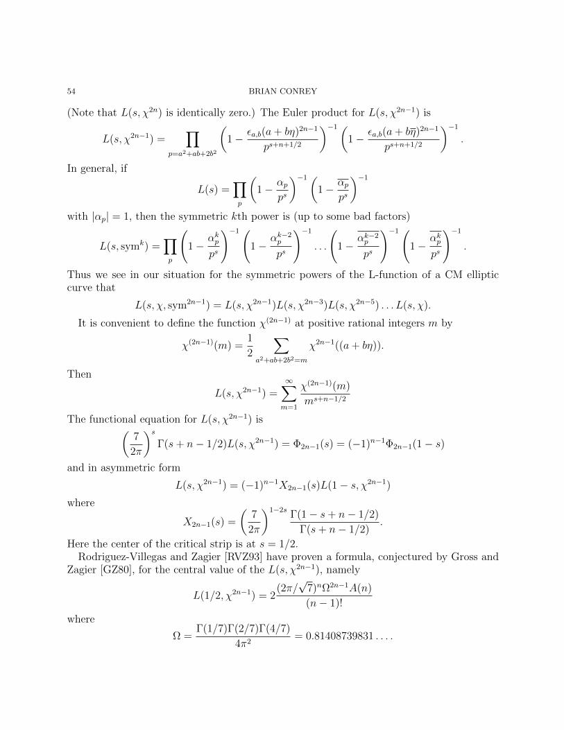
54 BRIAN CONREY
(Note that L(s, χ2n) is identically zero.) The Euler product for L(s, χ2n−1) is
L(s, χ2n−1) =∏
p=a2+ab+2b2
(1− εa,b(a+ bη)2n−1
ps+n+1/2
)−1(1− εa,b(a+ bη)2n−1
ps+n+1/2
)−1
.
In general, if
L(s) =∏p
(1− αp
ps
)−1(1− αp
ps
)−1
with |αp| = 1, then the symmetric kth power is (up to some bad factors)
L(s, symk) =∏p
(1−
αkpps
)−1(1−
αk−2p
ps
)−1
. . .
(1−
αk−2p
ps
)−1(1−
αkpps
)−1
.
Thus we see in our situation for the symmetric powers of the L-function of a CM ellipticcurve that
L(s, χ, sym2n−1) = L(s, χ2n−1)L(s, χ2n−3)L(s, χ2n−5) . . . L(s, χ).
It is convenient to define the function χ(2n−1) at positive rational integers m by
χ(2n−1)(m) =1
2
∑a2+ab+2b2=m
χ2n−1((a+ bη)).
Then
L(s, χ2n−1) =∞∑m=1
χ(2n−1)(m)
ms+n−1/2
The functional equation for L(s, χ2n−1) is(7
2π
)sΓ(s+ n− 1/2)L(s, χ2n−1) = Φ2n−1(s) = (−1)n−1Φ2n−1(1− s)
and in asymmetric form
L(s, χ2n−1) = (−1)n−1X2n−1(s)L(1− s, χ2n−1)
where
X2n−1(s) =
(7
2π
)1−2sΓ(1− s+ n− 1/2)
Γ(s+ n− 1/2).
Here the center of the critical strip is at s = 1/2.Rodriguez-Villegas and Zagier [RVZ93] have proven a formula, conjectured by Gross and
Zagier [GZ80], for the central value of the L(s, χ2n−1), namely
L(1/2, χ2n−1) = 2(2π/√
7)nΩ2n−1A(n)
(n− 1)!
where
Ω =Γ(1/7)Γ(2/7)Γ(4/7)
4π2= 0.81408739831 . . . .
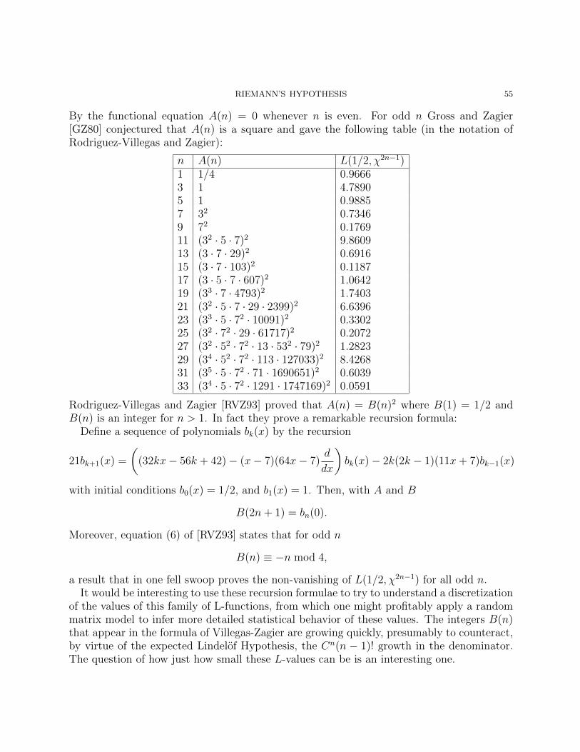
RIEMANN’S HYPOTHESIS 55
By the functional equation A(n) = 0 whenever n is even. For odd n Gross and Zagier[GZ80] conjectured that A(n) is a square and gave the following table (in the notation ofRodriguez-Villegas and Zagier):
n A(n) L(1/2, χ2n−1)1 1/4 0.96663 1 4.78905 1 0.98857 32 0.73469 72 0.176911 (32 · 5 · 7)2 9.860913 (3 · 7 · 29)2 0.691615 (3 · 7 · 103)2 0.118717 (3 · 5 · 7 · 607)2 1.064219 (33 · 7 · 4793)2 1.740321 (32 · 5 · 7 · 29 · 2399)2 6.639623 (33 · 5 · 72 · 10091)2 0.330225 (32 · 72 · 29 · 61717)2 0.207227 (32 · 52 · 72 · 13 · 532 · 79)2 1.282329 (34 · 52 · 72 · 113 · 127033)2 8.426831 (35 · 5 · 72 · 71 · 1690651)2 0.603933 (34 · 5 · 72 · 1291 · 1747169)2 0.0591
Rodriguez-Villegas and Zagier [RVZ93] proved that A(n) = B(n)2 where B(1) = 1/2 andB(n) is an integer for n > 1. In fact they prove a remarkable recursion formula:
Define a sequence of polynomials bk(x) by the recursion
21bk+1(x) =
((32kx− 56k + 42)− (x− 7)(64x− 7)
d
dx
)bk(x)− 2k(2k − 1)(11x+ 7)bk−1(x)
with initial conditions b0(x) = 1/2, and b1(x) = 1. Then, with A and B
B(2n+ 1) = bn(0).
Moreover, equation (6) of [RVZ93] states that for odd n
B(n) ≡ −n mod 4,
a result that in one fell swoop proves the non-vanishing of L(1/2, χ2n−1) for all odd n.It would be interesting to use these recursion formulae to try to understand a discretization
of the values of this family of L-functions, from which one might profitably apply a randommatrix model to infer more detailed statistical behavior of these values. The integers B(n)that appear in the formula of Villegas-Zagier are growing quickly, presumably to counteract,by virtue of the expected Lindelof Hypothesis, the Cn(n − 1)! growth in the denominator.The question of how just how small these L-values can be is an interesting one.
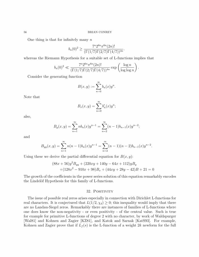
56 BRIAN CONREY
One thing is that for infinitely many n
bn(0)2 ≥ 7n26nπ6n(2n)!
(Γ(1/7)Γ(2/7)Γ(4/7))4n.
whereas the Riemann Hypothesis for a suitable set of L-functions implies that
bn(0)2 7n26nπ6n(2n)!
(Γ(1/7)Γ(2/7)Γ(4/7))4nexp
(log n
log log n
).
Consider the generating function
B(x, y) :=∞∑n=0
bn(x)yn.
Note that
Bx(x, y) =∞∑n=0
b′n(x)yn;
also,
By(x, y) =∞∑n=1
nbn(x)yn−1 =∞∑n=2
(n− 1)bn−1(x)yn−2;
and
Byy(x, y) =∞∑n=1
n(n− 1)bn(x)yn−1 =∞∑n=2
(n− 1)(n− 2)bn−1(x)yn−2.
Using these we derive the partial differential equation for B(x, y):
(88x+ 56)y2Byy + (220xy + 140y − 64x+ 112)yBy
+(128x2 − 910x+ 98)Bx + (44xy + 28y − 42)B + 21 = 0
The growth of the coefficients in the power series solution of this equation remarkably encodesthe Lindelof Hypothesis for this family of L-functions.
32. Positivity
The issue of possible real zeros arises especially in connection with Dirichlet L-functions forreal characters. It is conjectured that L(1/2, χd) ≥ 0; this inequality would imply that thereare no Landau-Siegel zeros. Remarkably there are instances of families of L-functions whereone does know the non-negativity - or even positivity - of the central value. Such is truefor example for primitive L-functions of degree 2 with no character, by work of Waldspurger[Wal81] and Kohnen and Zagier [KZ81], and Katok and Sarnak [KatS93]. For example,Kohnen and Zagier prove that if Lf (s) is the L-function of a weight 2k newform for the full
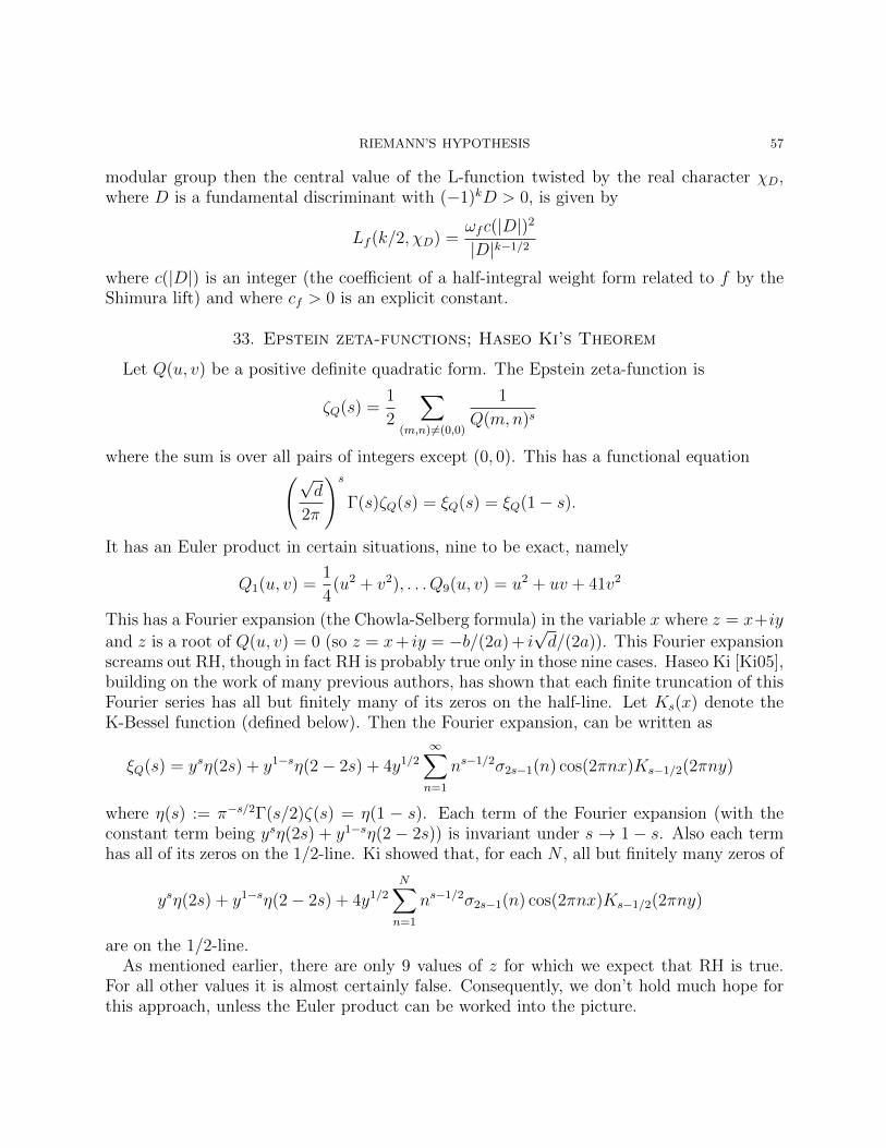
RIEMANN’S HYPOTHESIS 57
modular group then the central value of the L-function twisted by the real character χD,where D is a fundamental discriminant with (−1)kD > 0, is given by
Lf (k/2, χD) =ωfc(|D|)2
|D|k−1/2
where c(|D|) is an integer (the coefficient of a half-integral weight form related to f by theShimura lift) and where cf > 0 is an explicit constant.
33. Epstein zeta-functions; Haseo Ki’s Theorem
Let Q(u, v) be a positive definite quadratic form. The Epstein zeta-function is
ζQ(s) =1
2
∑(m,n)6=(0,0)
1
Q(m,n)s
where the sum is over all pairs of integers except (0, 0). This has a functional equation(√d
2π
)s
Γ(s)ζQ(s) = ξQ(s) = ξQ(1− s).
It has an Euler product in certain situations, nine to be exact, namely
Q1(u, v) =1
4(u2 + v2), . . . Q9(u, v) = u2 + uv + 41v2
This has a Fourier expansion (the Chowla-Selberg formula) in the variable x where z = x+iy
and z is a root of Q(u, v) = 0 (so z = x+ iy = −b/(2a) + i√d/(2a)). This Fourier expansion
screams out RH, though in fact RH is probably true only in those nine cases. Haseo Ki [Ki05],building on the work of many previous authors, has shown that each finite truncation of thisFourier series has all but finitely many of its zeros on the half-line. Let Ks(x) denote theK-Bessel function (defined below). Then the Fourier expansion, can be written as
ξQ(s) = ysη(2s) + y1−sη(2− 2s) + 4y1/2
∞∑n=1
ns−1/2σ2s−1(n) cos(2πnx)Ks−1/2(2πny)
where η(s) := π−s/2Γ(s/2)ζ(s) = η(1 − s). Each term of the Fourier expansion (with theconstant term being ysη(2s) + y1−sη(2− 2s)) is invariant under s → 1− s. Also each termhas all of its zeros on the 1/2-line. Ki showed that, for each N , all but finitely many zeros of
ysη(2s) + y1−sη(2− 2s) + 4y1/2
N∑n=1
ns−1/2σ2s−1(n) cos(2πnx)Ks−1/2(2πny)
are on the 1/2-line.As mentioned earlier, there are only 9 values of z for which we expect that RH is true.
For all other values it is almost certainly false. Consequently, we don’t hold much hope forthis approach, unless the Euler product can be worked into the picture.
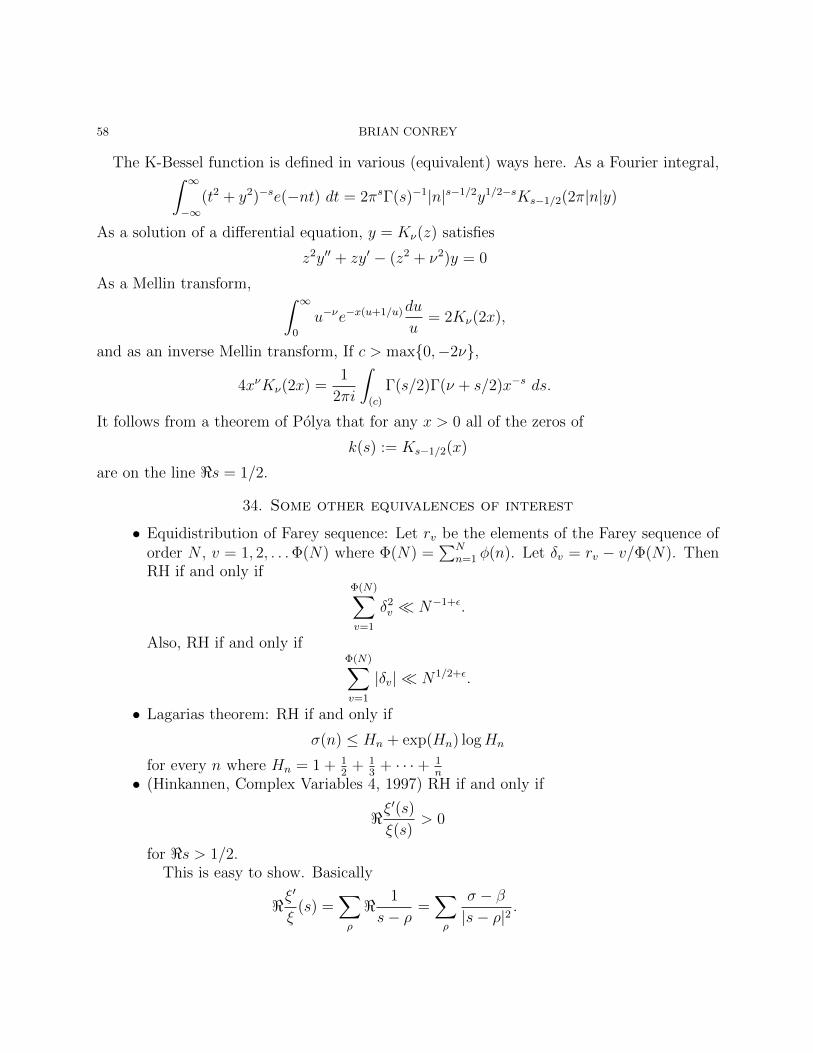
58 BRIAN CONREY
The K-Bessel function is defined in various (equivalent) ways here. As a Fourier integral,∫ ∞−∞
(t2 + y2)−se(−nt) dt = 2πsΓ(s)−1|n|s−1/2y1/2−sKs−1/2(2π|n|y)
As a solution of a differential equation, y = Kν(z) satisfies
z2y′′ + zy′ − (z2 + ν2)y = 0
As a Mellin transform, ∫ ∞0
u−νe−x(u+1/u)du
u= 2Kν(2x),
and as an inverse Mellin transform, If c > max0,−2ν,
4xνKν(2x) =1
2πi
∫(c)
Γ(s/2)Γ(ν + s/2)x−s ds.
It follows from a theorem of Polya that for any x > 0 all of the zeros of
k(s) := Ks−1/2(x)
are on the line <s = 1/2.
34. Some other equivalences of interest
• Equidistribution of Farey sequence: Let rv be the elements of the Farey sequence oforder N , v = 1, 2, . . .Φ(N) where Φ(N) =
∑Nn=1 φ(n). Let δv = rv − v/Φ(N). Then
RH if and only ifΦ(N)∑v=1
δ2v N−1+ε.
Also, RH if and only ifΦ(N)∑v=1
|δv| N1/2+ε.
• Lagarias theorem: RH if and only if
σ(n) ≤ Hn + exp(Hn) logHn
for every n where Hn = 1 + 12
+ 13
+ · · ·+ 1n
• (Hinkannen, Complex Variables 4, 1997) RH if and only if
<ξ′(s)
ξ(s)> 0
for <s > 1/2.This is easy to show. Basically
<ξ′
ξ(s) =
∑ρ
< 1
s− ρ=∑ρ
σ − β|s− ρ|2
.
RIEMANN’S HYPOTHESIS 59
If RH holds, then all β = 1/2 and so σ > 1/2 implies each term of the sum is positive.If there is a ρ = β + iγ with β > 1/2, then by choosing s = σ + iγ, the term in thesum corresponding to ρ is 1/(σ − β) which for σ very close to β but smaller than itwill cause the entire sum to be negative.• V. V. Volchkov has shown that RH is equivalent to the equality∫ ∞
0
∫ ∞1/2
1− 12y2
(1 + 4y2)3log(|ζ(x+ iy)|) dx dy = π
3− γ32
• Convergence of Carey’s series: RH if and only if
∞∑n=0
(n+
1
2
) ∣∣∣∣∣n∑k=0
c2n+1,2k+1
2k + 2log
(2k + 1
2k + 2
(−1)k B2k+2 (2π)2k+2
2 (2k + 2)!
)∣∣∣∣∣2
<∞
where cm,r denotes the coefficient of xr in the Legendre polynomial of degree m andBk is the kth Bernoulli number. Specifically,
c2n+1,2k+1 =(−1)n−k (2n+ 2k + 2)!
22n+1 (n− k)! (n+ k + 1)! (2k + 1)!
and
ζ (2k) =(−1)k+1 (2π)2k
2 (2k)!B2k
35. Zeros on the line
In this section we briefly describe the methods that have show that many zeros are on theline.
35.1. Simplest method. The simplest way to conclude that infinitely many zeros are onthe 1/2-line seems to be to contrast the behaviors of∣∣∣∣∫ T
0
Z(t) dt
∣∣∣∣and ∫ T
0
|Z(t)| dt.
We can show that these behave differently asymptotically as T → ∞ which implies thatthere are infinitely many zeros on the line. We easily have∫ T
0
|Z(t)| dt ≥∣∣∣∣∫ T
0
ζ(1/2 + it) dt
∣∣∣∣ ∼ T
by moving the path of integration in the latter integral to the right of 1 and integrating termby term. On the other hand ∫ T
0
Z(t) dt
60 BRIAN CONREY
has substantial cancelation because of the oscillations in χ(1 − s)−1/2 ∼ exp(it/2 log t) andcan be bounded from above in various ways by T 3/4 for example.
Incidentally, this assertion has not been proven for degree 3 L-functions.
35.2. Hardy and Littlewood’s method. The above can be strengthened to show thatthere are T zeros on the line up to a height T . Basically one compares∫ T
0
∣∣∣∣∫ t+H
t
Z(u) du
∣∣∣∣ dtwith ∫ T
0
(∫ t+H
t
|Z(u)| du)dt.
35.3. Siegel’s method. Siegel employed a formula found in Riemann’s notes
π−s/2Γ(s/2)ζ(s) = π−s/2Γ(s/2)f(s) + π−1−s2 Γ((1− s)/2)f(1− s)
where
f(s) =
∫L
x−seπix2
eπix − e−πixdx
(here L is a line of slope −1 that passes through 1/2) to assert that ζ(1/2+ it) = 0 wheneverthe argument of
π−s/2Γ(s/2)f(s)
is congruent to π/2 modulo π. After applying the argument principle, the problem boilsdown to showing that the entire function f(s) has many zeros to the left of the 1/2-line.Most of the zeros seem to be near the 1/2-line which makes this proposition seem daunting.But through some quite sophisticated analysis Siegel is able to show that the entire f(s)actually has T zeros to the left of the 0-line at a height smaller than T . In this way hededuces at least T zeros on the line for ζ(s).
35.4. Selberg’s method. This is like the Hardy-Littlewood method except that in placeof Z(t) one uses Z(t)|η(t)|2 where η(t) is an approximation to ζ(1/2 + it)−1/2; thus |η(t)|2acts as a “mollifier” for ζ(1/2 + it) to mitigate the loss of a log T that occurs when Cauchy’sinequality is invoked in the Hardy-Littlewood method.
35.5. Levinson’s method. This is like Siegel’s method except that f(s) is basically re-placed by ζ ′(1 − s) and a mollifier is used to avoid losing a logarithm and Littlewood’slemma is invoked to give an upper bound for the number of zeros of ζ ′(1− s) with real partlarger than 1/2. Now the analysis is delicate; it’s clear from the start that one will obtain alower bound of the right order of magnitude but the sign of that magnitude is in question.At the end of the calculation one might conclude that at least −10% of the zeros are onthe critical line. Fortunately, Levinson gets 1/3 of the zeros on the line; a very respectableresult.
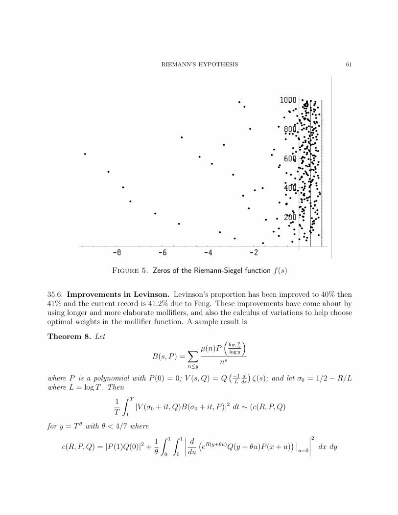
RIEMANN’S HYPOTHESIS 61
Figure 5. Zeros of the Riemann-Siegel function f(s)
35.6. Improvements in Levinson. Levinson’s proportion has been improved to 40% then41% and the current record is 41.2% due to Feng. These improvements have come about byusing longer and more elaborate mollifiers, and also the calculus of variations to help chooseoptimal weights in the mollifier function. A sample result is
Theorem 8. Let
B(s, P ) =∑n≤y
µ(n)P(
log yn
log y
)ns
where P is a polynomial with P (0) = 0; V (s,Q) = Q(−1L
dds
)ζ(s); and let σ0 = 1/2 − R/L
where L = log T . Then
1
T
∫ T
1
|V (σ0 + it, Q)B(σ0 + it, P )|2 dt ∼ (c(R,P,Q)
for y = T θ with θ < 4/7 where
c(R,P,Q) = |P (1)Q(0)|2 +1
θ
∫ 1
0
∫ 1
0
∣∣∣∣ ddu (eR(y+θu)Q(y + θu)P (x+ u)) ∣∣
u=0
∣∣∣∣2 dx dy

62 BRIAN CONREY
The length θ of the mollifier is critical here; Farmer [Far93] has conjectured that theabove asymptotic formula holds true for arbitrary fixed θ; this is called the “long mollifiers”conjecture. It would imply that 100% of the zeros of ζ(s) are on the critical line. In fact,Bettin (unpublished) has an argument that the long mollifiers conjecture implies RH.
A qualitative improvement in Levinson’s method is that the proportion of zeros on thecritical line of ξ(n)(s) the n-th derivative of the Riemann xi-function approaches 1 as n→∞.So, in some ways Levinson’s method is very satisfying. Also, Levinson’s method can bearranged to produce simple zeros, a fact observed independently by Selberg (unpublished)and Heath-Brown [H-B79]. It is known [BCY11] that at least 40.5% of the zeros of ζ(s) aresimple and on the critical line.
36. Critical zeros of other L-functions
Hafner has used Selberg’s method to prove that a positive proportion of the zeros of degree2 L-functions are on the critical line. Levinson’s method doesn’t quite work for degree 2 L-functions but it does give bounds for the multiplicity of zeros, [Far94].
Conrey, Iwaniec and Soundararajan [CIS13] have shown that at least 60% of the collectivezeros of all Dirichlet L-functions are on the critical line; similarly at least 36% of all thetwists by Dirichlet characters of a fixed degree 2 L-function are on the critical line; and atleast 0.5% of all the twists by Dirichlet characters of a fixed degree 3 L-function are on thecritical line.
Work on real zeros of Dirichlet L-functions is extremely interesting in this context. Insome ways this study is a microcosm of work on the Riemann Hypothesis.
Soundararajan [Sou00] has shown that at least 7/8 of these L-functions don’t vanish atthe center.
Conrey and Soundararajan [CS02] have shown that at least 20% of such L-functions haveno real zeros.
There is a simple approach using Fekete polynomials
Fχd(t) =
|d|−1∑n=1
χd(n)tn;
if Fχd(t) > 0 for 0 < t < 1 then L(s, χd) has no positive real zeros. But this idea fails quickly,in particular for d = −163. In fact Montgomery and Baker proved that L(s, χd) oscillatesquite a lot on the real interval from 0 to 1, likely as many as log log |d| times. Chowlaand Selberg [ChSe67] considered the Dedekind zeta function ζ(s)L(s, χd) for the imaginary
quadratic field Q(√d) (with d < 0) and identified it as an Epstein zeta-function for which
they found an explicit Fourier expansion which was used to prove that the L(s, χ−163) hasno positive real zeros. Bateman and Grosswald [BG64] identified the Bessel functions in theformula to give the following: Suppose that d = b2 − 4ac < 0 and let
Z(s) =1
2
∑(m,n) 6=(0,0)
1
am2 + bmn+ cn2)s.
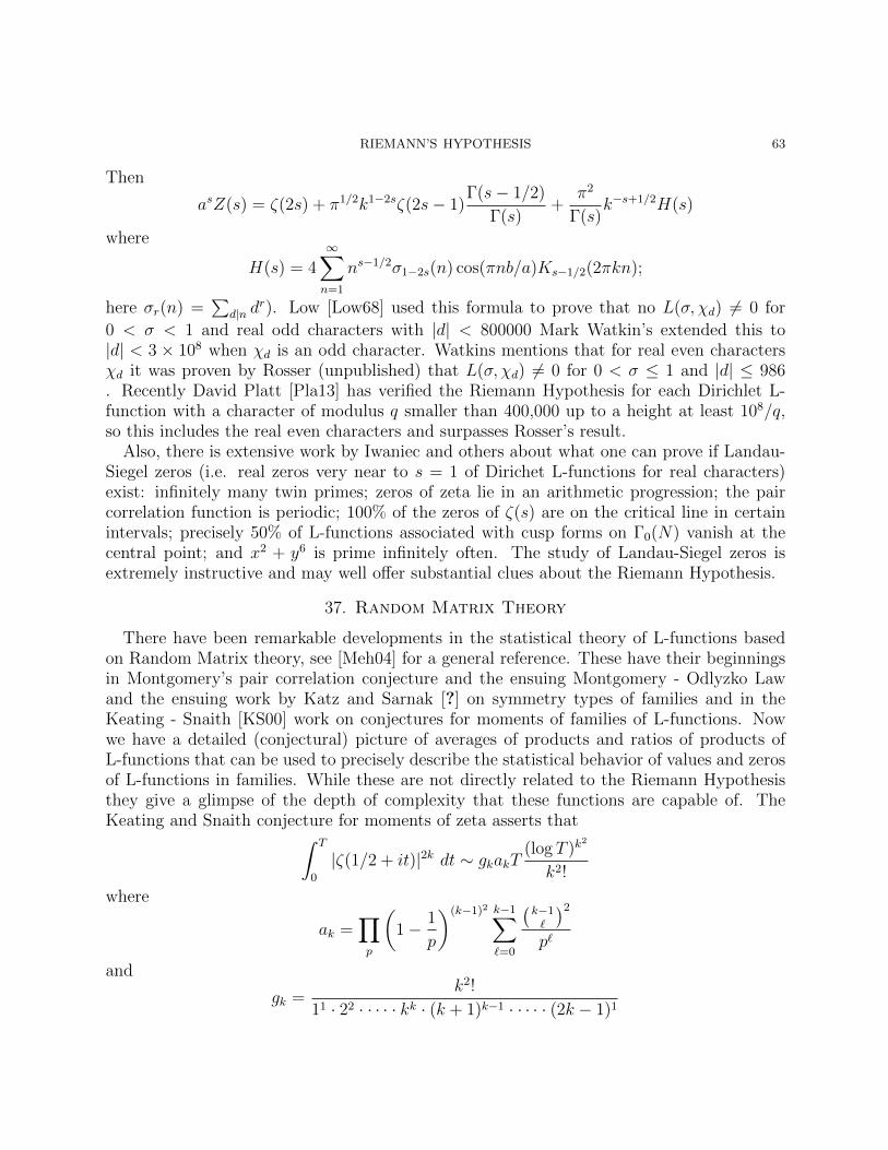
RIEMANN’S HYPOTHESIS 63
Then
asZ(s) = ζ(2s) + π1/2k1−2sζ(2s− 1)Γ(s− 1/2)
Γ(s)+
π2
Γ(s)k−s+1/2H(s)
where
H(s) = 4∞∑n=1
ns−1/2σ1−2s(n) cos(πnb/a)Ks−1/2(2πkn);
here σr(n) =∑
d|n dr). Low [Low68] used this formula to prove that no L(σ, χd) 6= 0 for
0 < σ < 1 and real odd characters with |d| < 800000 Mark Watkin’s extended this to|d| < 3 × 10⁸ when χd is an odd character. Watkins mentions that for real even charactersχd it was proven by Rosser (unpublished) that L(σ, χd) 6= 0 for 0 < σ ≤ 1 and |d| ≤ 986. Recently David Platt [Pla13] has verified the Riemann Hypothesis for each Dirichlet L-function with a character of modulus q smaller than 400,000 up to a height at least 108/q,so this includes the real even characters and surpasses Rosser’s result.
Also, there is extensive work by Iwaniec and others about what one can prove if Landau-Siegel zeros (i.e. real zeros very near to s = 1 of Dirichet L-functions for real characters)exist: infinitely many twin primes; zeros of zeta lie in an arithmetic progression; the paircorrelation function is periodic; 100% of the zeros of ζ(s) are on the critical line in certainintervals; precisely 50% of L-functions associated with cusp forms on Γ0(N) vanish at thecentral point; and x2 + y6 is prime infinitely often. The study of Landau-Siegel zeros isextremely instructive and may well offer substantial clues about the Riemann Hypothesis.
37. Random Matrix Theory
There have been remarkable developments in the statistical theory of L-functions basedon Random Matrix theory, see [Meh04] for a general reference. These have their beginningsin Montgomery’s pair correlation conjecture and the ensuing Montgomery - Odlyzko Lawand the ensuing work by Katz and Sarnak [?] on symmetry types of families and in theKeating - Snaith [KS00] work on conjectures for moments of families of L-functions. Nowwe have a detailed (conjectural) picture of averages of products and ratios of products ofL-functions that can be used to precisely describe the statistical behavior of values and zerosof L-functions in families. While these are not directly related to the Riemann Hypothesisthey give a glimpse of the depth of complexity that these functions are capable of. TheKeating and Snaith conjecture for moments of zeta asserts that∫ T
0
|ζ(1/2 + it)|2k dt ∼ gkakT(log T )k
2
k2!
where
ak =∏p
(1− 1
p
)(k−1)2 k−1∑`=0
(k−1`
)2
p`
and
gk =k2!
11 · 22 · · · · · kk · (k + 1)k−1 · · · · · (2k − 1)1
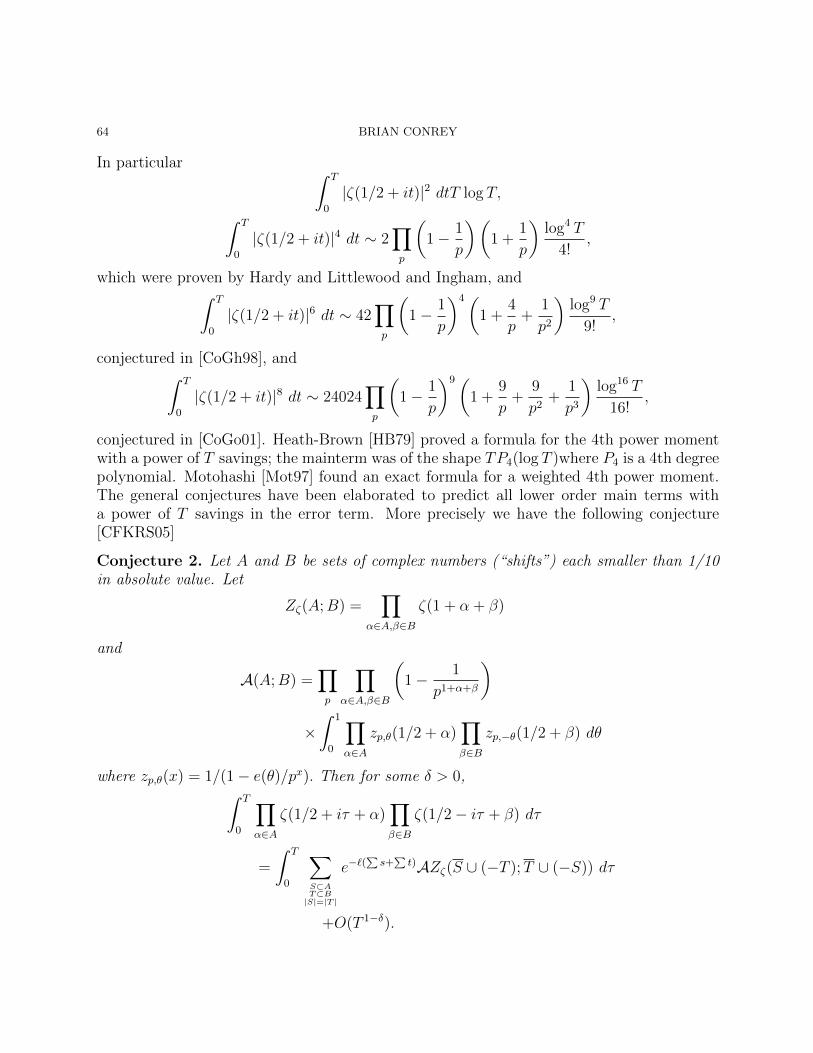
64 BRIAN CONREY
In particular ∫ T
0
|ζ(1/2 + it)|2 dtT log T,∫ T
0
|ζ(1/2 + it)|4 dt ∼ 2∏p
(1− 1
p
)(1 +
1
p
)log4 T
4!,
which were proven by Hardy and Littlewood and Ingham, and∫ T
0
|ζ(1/2 + it)|6 dt ∼ 42∏p
(1− 1
p
)4(1 +
4
p+
1
p2
)log9 T
9!,
conjectured in [CoGh98], and∫ T
0
|ζ(1/2 + it)|8 dt ∼ 24024∏p
(1− 1
p
)9(1 +
9
p+
9
p2+
1
p3
)log16 T
16!,
conjectured in [CoGo01]. Heath-Brown [HB79] proved a formula for the 4th power momentwith a power of T savings; the mainterm was of the shape TP4(log T )where P4 is a 4th degreepolynomial. Motohashi [Mot97] found an exact formula for a weighted 4th power moment.The general conjectures have been elaborated to predict all lower order main terms witha power of T savings in the error term. More precisely we have the following conjecture[CFKRS05]
Conjecture 2. Let A and B be sets of complex numbers (“shifts”) each smaller than 1/10in absolute value. Let
Zζ(A;B) =∏
α∈A,β∈B
ζ(1 + α + β)
and
A(A;B) =∏p
∏α∈A,β∈B
(1− 1
p1+α+β
)
×∫ 1
0
∏α∈A
zp,θ(1/2 + α)∏β∈B
zp,−θ(1/2 + β) dθ
where zp,θ(x) = 1/(1− e(θ)/px). Then for some δ > 0,∫ T
0
∏α∈A
ζ(1/2 + iτ + α)∏β∈B
ζ(1/2− iτ + β) dτ
=
∫ T
0
∑S⊂AT⊂B|S|=|T |
e−`(∑s+
∑t)AZζ(S ∪ (−T );T ∪ (−S)) dτ
+O(T 1−δ).
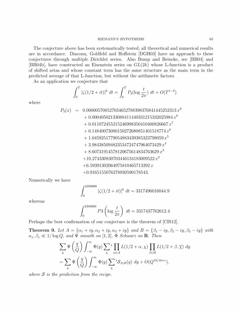
RIEMANN’S HYPOTHESIS 65
The conjecture above has been systematically tested; all theoretical and numerical resultsare in accordance. Diaconu, Goldfeld and Hoffstein [DGH03] have an approach to theseconjectures through multiple Dirichlet series. Also Bump and Beineke, see [BB04] and[BB04b], have constructed an Eisenstein series on GL(2k) whose L-function is a productof shifted zetas and whose constant term has the same structure as the main term in thepredicted average of that L-function, but without the arithmetic factors.
As an application we conjecture that∫ T
0
|ζ(1/2 + it)|6 dt =
∫ T
0
P3(logt
2π) dt+O(T 1−δ)
where
P3(x) = 0.000005708527034652788398376841445252313x9
+ 0.00040502133088411440331215332025984x8
+ 0.011072455215246998350410400826667x7
+ 0.14840073080150272680851401518774x6
+ 1.0459251779054883439385323798059x5
+ 3.984385094823534724747964073429 x4
+ 8.60731914578120675614834763629 x3
+10.274330830703446134183009522 x2
+6.59391302064975810465713392 x
+0.9165155076378930590178543.
Numerically we have ∫ 2350000
0
|ζ(1/2 + it)|6 dt = 3317496016044.9
whereas ∫ 2350000
0
P3
(log
t
2π
)dt = 3317437762612.4
Perhaps the best confirmation of our conjecture is the theorem of [CIS12].
Theorem 9. Let A = α1 + iy, α2 + iy, α3 + iy and B = β1 − iy, β2 − iy, β3 − iy withαj, βj 1/ logQ, and Ψ smooth on [1, 2], Φ Schwarz on R. Then∑
q
Ψ
(q
Q
)∫ ∞−∞
Φ(y)∑χ
[∏α∈A
L(1/2 + α, χ)∏β∈B
L(1/2 + β, χ) dy
=∑q
Ψ
(q
Q
)∫ ∞−∞
Φ(y)∑χ
[SA;B(q) dy +O(Q19/10+ε).
where S is the prediction from the recipe.
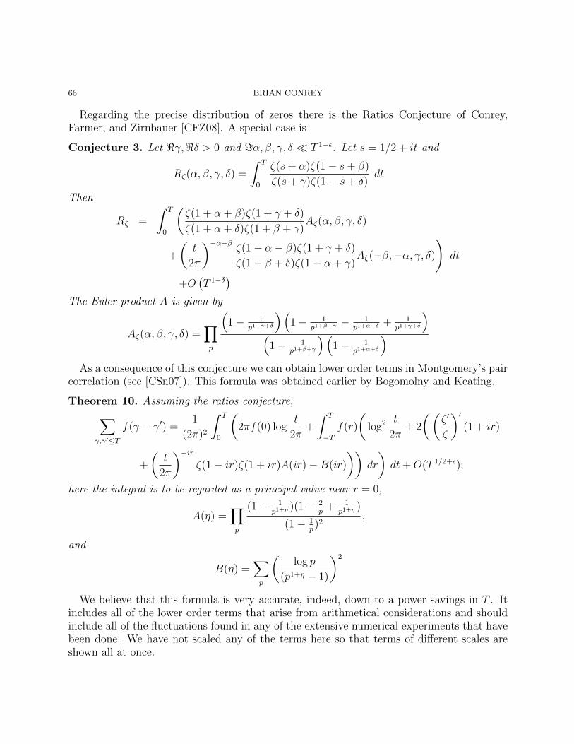
66 BRIAN CONREY
Regarding the precise distribution of zeros there is the Ratios Conjecture of Conrey,Farmer, and Zirnbauer [CFZ08]. A special case is
Conjecture 3. Let <γ,<δ > 0 and =α, β, γ, δ T 1−ε. Let s = 1/2 + it and
Rζ(α, β, γ, δ) =
∫ T
0
ζ(s+ α)ζ(1− s+ β)
ζ(s+ γ)ζ(1− s+ δ)dt
Then
Rζ =
∫ T
0
(ζ(1 + α + β)ζ(1 + γ + δ)
ζ(1 + α + δ)ζ(1 + β + γ)Aζ(α, β, γ, δ)
+
(t
2π
)−α−βζ(1− α− β)ζ(1 + γ + δ)
ζ(1− β + δ)ζ(1− α + γ)Aζ(−β,−α, γ, δ)
)dt
+O(T 1−δ)
The Euler product A is given by
Aζ(α, β, γ, δ) =∏p
(1− 1
p1+γ+δ
)(1− 1
p1+β+γ− 1
p1+α+δ+ 1
p1+γ+δ
)(
1− 1p1+β+γ
)(1− 1
p1+α+δ
)As a consequence of this conjecture we can obtain lower order terms in Montgomery’s pair
correlation (see [CSn07]). This formula was obtained earlier by Bogomolny and Keating.
Theorem 10. Assuming the ratios conjecture,∑γ,γ′≤T
f(γ − γ′) =1
(2π)2
∫ T
0
(2πf(0) log
t
2π+
∫ T
−Tf(r)
(log2 t
2π+ 2
((ζ ′
ζ
)′(1 + ir)
+
(t
2π
)−irζ(1− ir)ζ(1 + ir)A(ir)−B(ir)
))dr
)dt+O(T 1/2+ε);
here the integral is to be regarded as a principal value near r = 0,
A(η) =∏p
(1− 1p1+η
)(1− 2p
+ 1p1+η
)
(1− 1p)2
,
and
B(η) =∑p
(log p
(p1+η − 1)
)2
We believe that this formula is very accurate, indeed, down to a power savings in T . Itincludes all of the lower order terms that arise from arithmetical considerations and shouldinclude all of the fluctuations found in any of the extensive numerical experiments that havebeen done. We have not scaled any of the terms here so that terms of different scales areshown all at once.
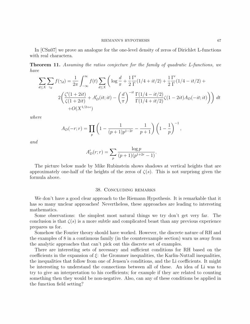
RIEMANN’S HYPOTHESIS 67
In [CSn07] we prove an analogue for the one-level density of zeros of Dirichlet L-functionswith real charactera.
Theorem 11. Assuming the ratios conjecture for the family of quadratic L-functions, wehave∑
d≤X
∑γd
f(γd) =1
2π
∫ ∞−∞
f(t)∑d≤X
(log
d
π+
1
2
Γ′
Γ(1/4 + it/2) +
1
2
Γ′
Γ(1/4− it/2) +
2
(ζ ′(1 + 2it)
ζ(1 + 2it)+ A′D(it; it)−
(d
π
)−itΓ(1/4− it/2)
Γ(1/4 + it/2)ζ(1− 2it)AD(−it; it)
))dt
+O(X1/2+ε)
where
AD(−r; r) =∏p
(1− 1
(p+ 1)p1−2r− 1
p+ 1
)(1− 1
p
)−1
,
and
A′D(r; r) =∑p
log p
(p+ 1)(p1+2r − 1).
The picture below made by Mike Rubinstein shows shadows at vertical heights that areapproximately one-half of the heights of the zeros of ζ(s). This is not surprisng given theformula above.
38. Concluding remarks
We don’t have a good clear approach to the Riemann Hypothesis. It is remarkable that ithas so many unclear approaches! Nevertheless, these approaches are leading to interestingmathematics.
Some observations: the simplest most natural things we try don’t get very far. Theconclusion is that ζ(s) is a more subtle and complicated beast than any previous experienceprepares us for.
Somehow the Fourier theory should have worked. However, the discrete nature of RH andthe examples of 8 in a continuous family (in the counterexample section) warn us away fromthe analytic approaches that can’t pick out this discrete set of examples.
There are interesting sets of necessary and sufficient conditions for RH based on thecoefficients in the expansion of ξ: the Grommer inequalities, the Karlin-Nuttall inequalities,the inequalities that follow from one of Jensen’s conditions, and the Li coefficients. It mightbe interesting to understand the connections between all of these. An idea of Li was totry to give an interpretation to his coefficients; for example if they are related to countingsomething then they would be non-negative. Also, can any of these conditions be applied inthe function field setting?

68 BRIAN CONREY
Figure 6. Zeros of L(s, χd)
We do need the Euler product. The straight conjecture about almost periodicity andgeneral Dirichlet series, while intriguing, is probably really hard.
The Rodriguez-Villegas and Zagier recursion formula is extremely tantalizing! And thereare connections with this approach and with a continuous family of p-adic Eisenstein seriesthat is worth investigation.
We have mentioned but not discussed the Stepanov - Bombieri proof of Weil’s theorem.It is very interesting and potentially brings a new theory and techniques from transcenden-tal number theory into play. In general one should possibly try to find classical analyticapproaches that work to prove Weil’s theorem.
We have not mentioned the Langlands’ program for automorphic representations. A sam-ple conjecture is that the L-function attached to any symmetric power of another L-functionis itself meromorphic and has a functional equation. Unfortunately, even if we knew such apowerful statement to be true we still wouldn’t know how to use it to deduce RH.
Also we haven’t written about Iwaniec’s ideas to use families of elliptic curves which haverank > 1 and root numbers which capture the Mobius function. The idea of using theexisting landscape of L-functions with multiple zeros to say something about the Riemannzeta -function is very attractive. For example:
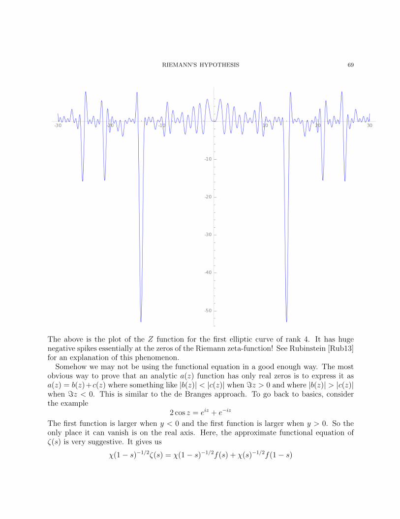
RIEMANN’S HYPOTHESIS 69
The above is the plot of the Z function for the first elliptic curve of rank 4. It has hugenegative spikes essentially at the zeros of the Riemann zeta-function! See Rubinstein [Rub13]for an explanation of this phenomenon.
Somehow we may not be using the functional equation in a good enough way. The mostobvious way to prove that an analytic a(z) function has only real zeros is to express it asa(z) = b(z)+c(z) where something like |b(z)| < |c(z)| when =z > 0 and where |b(z)| > |c(z)|when =z < 0. This is similar to the de Branges approach. To go back to basics, considerthe example
2 cos z = eiz + e−iz
The first function is larger when y < 0 and the first function is larger when y > 0. So theonly place it can vanish is on the real axis. Here, the approximate functional equation ofζ(s) is very suggestive. It gives us
χ(1− s)−1/2ζ(s) = χ(1− s)−1/2f(s) + χ(s)−1/2f(1− s)
70 BRIAN CONREY
which essentially expresses ζ(s) as a sum of complex conjugates on the 1/2-line. Unfortu-nately it is not the case that one of these functions dominates in half of the plane. In factthe entire function f(s) seems to have infinitely many zeros on each side of the 1/2-line.Nevertheless Siegel used the above as a starting point for a proof that ζ(s) has T zeros onthe critical line up to a height T . Levinson’s starting point is also a decomposition of thisform. Differentiating H(s)ζ(s) = H(1− s)ζ(1− s) (where H(s) = π−s/2Γ(s/2)) we obtain
H(s)
(H ′
H(s) +
H ′
H(1− s)
)ζ(s) = −H(s)ζ ′(s)−H ′(1− s)ζ ′(1− s)
which effectively gives ζ(s) as a sum of complex conjugates in the critical line. This time,by Speiser’s theorem (as proven by Montgomery and Vaughan) one of these functions doesdominate. However, it is difficult to see how to prove this. Nevertheless Levinson uses thisas a starting point in his proof that at least one-third of the zeros are on the critical line.
The decomposition of the Fourier integral by the functional equation is another example.Perhaps it could be more useful. Perhaps start with the Lτ (s) so as to avoid the pole ats = 1. Also, perhaps the infinite product for ∆ could be useful now. Maybe use a circlemethod/saddle point method to analyze the ensuing functions near rational points with smalldenominator; then prove the desired inequality. However, again the counterexample of theeight warns us away.
Another possibility is to try to use the “2” that is everywhere, especially in approaches tothe Landau-Siegel zero. One could try to do long mollifiers, with optimal coefficients thatinvolve a smoothed Mobius function; then turn the tail of the sum into a sum over zeros;manipulate that somehow by a transform; then turn it back into a sum like one startedwith. In this way estimate a long mollification. This “2” arises in Selberg’s work whenhe bounds S(T ) point-wise by a Dirichlet polynomial (he bounds the sum over zeros by aDirichlet polynomial); see also Soundararajan’s proof of the upper bound for moments ofζ(s) (contingent on RH). Perhaps it is the same two that appears in Brun-Titchmarsh upperbounds for primes in arithmetic progressions.
In the Nyman-Beurling approach or the long mollifier approach one should probably tryto make use of the reciprocity formula for the cotangent sum.
A new powerful tool might be the theory of stable polynomials (see the references toBranden and Borcea). There are examples of how these get used in the proof of the Lee-yang theorem and in the recent proof of the Kadison-Singer theorem. They involve functionsof several variables but apply to problems in one variable.
Finally I want to mention Random Matrix Theory. Over the last 15 years we have de-veloped incredibly precise descriptions of statistics of families of L-functions; these includethings like moments in families with power savings and statistics of zeros, like pair correla-tions, again with power savings. The conjectures in the end are very symmetric and easy todescribe though they are admittedly combinatorially complicated. These conjectures leadthe way sometimes to proofs. For example in the work [CIS12] on the sixth moment of Dirich-let L-functions. The rigorous proofs involve spectacular combinatorial maneuvers. Knowingwhere we are headed is the thing that keeps us going. One thing we have learned is that
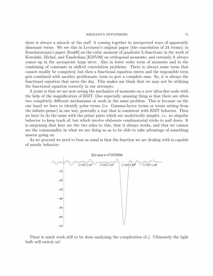
RIEMANN’S HYPOTHESIS 71
there is always a miracle at the end! A coming together in unexpected ways of apparentlydissonant terms. We see this in Levinson’s original paper (the cancelation of 24 terms); inSoundararajan’s paper [Sou00] on the cubic moment of quadratic L-functions; in the work ofKowalski, Michel, and Vanderkam [KMV00] on orthogonal moments; and certainly it alwayscomes up in the asymptotic large sieve. Also in lower order term of moments and in thecombining of constants in shifted convolution problems. There is always some term thatcannot readily be computed; but then a functional equation enters and the impossible termgets combined with another problematic term to give a complete sum. So, it is always thefunctional equation that saves the day. This makes me think that we may not be utilizingthe functional equation correctly in our attempts.
A point is that we are now seeing the mechanics of moments on a new ultra-fine scale withthe help of the magnification of RMT. One especially amazing thing is that there are oftentwo completely different mechanisms at work in the same problem. This is because on theone hand we have to identify polar terms (i.e. Gamma-factor terms or terms arising fromthe infinite-prime) in one way, generally a way that is consistent with RMT behavior. Thenwe have to do the same with the prime parts which are analytically simpler, i.e. no singularbehavior to keep track of, but which involve elaborate combinatorial tricks to nail down. Itis surprising that here are the two sides to this, that it always works, and that we cannotsee the commonality in what we are doing so as to be able to take advantage of somethingunseen going on.
As we proceed we need to bear in mind is that the function we are dealing with is capableof unruly behavior:
3.7187´108
3.7187´108
3.7187´108
3.7187´108
-70
-60
-50
-40
-30
-20
-10
ZHtL near t=371870204
There is much work still to be done analyzing the complexities of ζ. Ultimately the lightbulb will switch on!

72 BRIAN CONREY
References
[Alt68] Ronald Alter. On a necessary condition for the validity of the Riemann hypothesis for functionsthat generalize the Riemann zeta function. Trans. Amer. Math. Soc. 130 1968 55–74.
[Bac18] R. Backlund. Uber die Nullstellen der Riemannschen Zetafunktion, Acta Mathematica 41 (1918),345–75.
[B-D93] L. Baez-Duarte. On Beurling’s real variable reformulation of the Riemann hypothesis. Adv. Math.101 (1993), no. 1, 10–30.
[B-D02] Luis Baez-Duarte. New versions of the Nyman-Beurling criterion for the Riemann hypothesis.Int. J. Math. Math. Sci. 31 (2002), no. 7, 387–406.
[B-D03] L. Baez-Duarte, On Maslankas representation for the Riemann zeta function, math.NT/0307214(2003).
[B-D03b] Luis Baez-Duarte. A strengthening of the Nyman-Beurling criterion for the Riemann hypothesis.Atti Accad. Naz. Lincei Cl. Sci. Fis. Mat. Natur. Rend. Lincei (9) Mat. Appl. 14 (2003), no. 1,5–11.
[B-D05] L. Baez-Duarte, A sequential Riesz-like criterion for the Riemann Hypothesis, International Jour-nal of Mathematics and Mathematical Sciences 21, (2005) 3527- 3537.
[B-D05b] Luis Baez-Duarte. A general strong Nyman-Beurling criterion for the Riemann hypothesis. Publ.Inst. Math. (Beograd) (N.S.) 78(92) (2005), 117–125.
[BBLS00] Luis Baez-Duarte, Michel Balazard, Bernard Landreau, Eric Saias. Notes sur la fonction ζ deRiemann. III. (French) [Notes on the Riemann ζ-function. III] Adv. Math. 149 (2000), no. 1,130–144.
[Bag06] Bhaskar Bagchi. On Nyman, Beurling and Baez-Duarte’s Hilbert space reformulation ofthe Riemann hypothesis. Proc. Indian Acad. Sci. Math. Sci. 116 (2006), no. 2, 137–146.math.NT/0607733
[Bal02] Michel Balazard. Completeness problems and the Riemann hypothesis: an annotated bibliogra-phy. Number theory for the millennium, I (Urbana, IL, 2000), 21–48, A K Peters, Natick, MA,2002.
[BS98] Michel Balazard, Eric Saias. Notes sur la fonction ζ de Riemann. 1. (French) [Notes on theRiemann ζ-function. 1] Adv. Math. 139 (1998), no. 2, 310–321.
[BS00] Michel Balazard, Eric Saias. The Nyman-Beurling equivalent form for the Riemann hypothesis.Expo. Math. 18 (2000), no. 2, 131–138.
[BS04] Michel Balazard, Eric Saias. Notes sur la fonction ζ de Riemann. IV. Adv. Math. 188 (2004), no.1, 69–86.
[BSY99] Michel Balazard, Eric Saias, Marc Yor. Notes sur la fonction ζ de Riemann. II. Adv. Math. 143(1999), no. 2, 284–287.
[BFP89] Wayne W. Barrett, Rodney W. Forcade, Andrew D. Pollington. On the spectral radius of a (0, 1)matrix related to Mertens’ function. Proceedings of the Victoria Conference on CombinatorialMatrix Analysis (Victoria, BC, 1987). Linear Algebra Appl. 107 (1988), 151–159.
[BG64] P. T. Bateman, E. Grosswald. On Epstein’s zeta function. Acta Arith. 9 1964 365-373.[BB04] Jennifer Beineke, Daniel Bump. Moments of the Riemann zeta function and Eisenstein series. I.
J. Number Theory 105 (2004), no. 1, 150-174. More link[BB04b] Jennifer Beineke, Daniel Bump. Moments of the Riemann zeta function and Eisenstein series. II.
J. Number Theory 105 (2004), no. 1, 175-191.[BM06] S. Beltraminelli and D. Merlini, The criteria of Riesz, Hardy-Littlewood et al. for the Riemann
hypothesis revisited using similar functions, math.NT/0601138 (2006).[BK99] M. V. Berry, J. P. Keating. The Riemann zeros and eigenvalue asymptotics. SIAM Rev. 41 (1999),
no. 2, 236-266
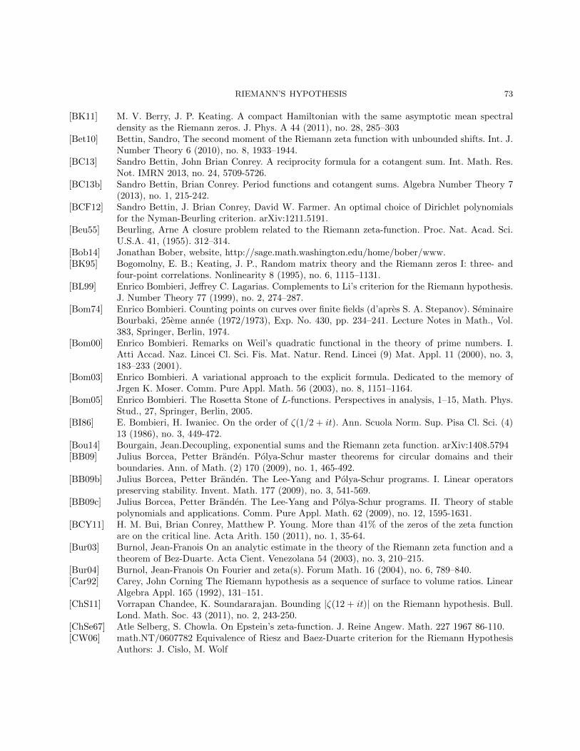
RIEMANN’S HYPOTHESIS 73
[BK11] M. V. Berry, J. P. Keating. A compact Hamiltonian with the same asymptotic mean spectraldensity as the Riemann zeros. J. Phys. A 44 (2011), no. 28, 285–303
[Bet10] Bettin, Sandro, The second moment of the Riemann zeta function with unbounded shifts. Int. J.Number Theory 6 (2010), no. 8, 1933–1944.
[BC13] Sandro Bettin, John Brian Conrey. A reciprocity formula for a cotangent sum. Int. Math. Res.Not. IMRN 2013, no. 24, 5709-5726.
[BC13b] Sandro Bettin, Brian Conrey. Period functions and cotangent sums. Algebra Number Theory 7(2013), no. 1, 215-242.
[BCF12] Sandro Bettin, J. Brian Conrey, David W. Farmer. An optimal choice of Dirichlet polynomialsfor the Nyman-Beurling criterion. arXiv:1211.5191.
[Beu55] Beurling, Arne A closure problem related to the Riemann zeta-function. Proc. Nat. Acad. Sci.U.S.A. 41, (1955). 312–314.
[Bob14] Jonathan Bober, website, http://sage.math.washington.edu/home/bober/www.[BK95] Bogomolny, E. B.; Keating, J. P., Random matrix theory and the Riemann zeros I: three- and
four-point correlations. Nonlinearity 8 (1995), no. 6, 1115–1131.[BL99] Enrico Bombieri, Jeffrey C. Lagarias. Complements to Li’s criterion for the Riemann hypothesis.
J. Number Theory 77 (1999), no. 2, 274–287.[Bom74] Enrico Bombieri. Counting points on curves over finite fields (d’apres S. A. Stepanov). Seminaire
Bourbaki, 25eme annee (1972/1973), Exp. No. 430, pp. 234–241. Lecture Notes in Math., Vol.383, Springer, Berlin, 1974.
[Bom00] Enrico Bombieri. Remarks on Weil’s quadratic functional in the theory of prime numbers. I.Atti Accad. Naz. Lincei Cl. Sci. Fis. Mat. Natur. Rend. Lincei (9) Mat. Appl. 11 (2000), no. 3,183–233 (2001).
[Bom03] Enrico Bombieri. A variational approach to the explicit formula. Dedicated to the memory ofJrgen K. Moser. Comm. Pure Appl. Math. 56 (2003), no. 8, 1151–1164.
[Bom05] Enrico Bombieri. The Rosetta Stone of L-functions. Perspectives in analysis, 1–15, Math. Phys.Stud., 27, Springer, Berlin, 2005.
[BI86] E. Bombieri, H. Iwaniec. On the order of ζ(1/2 + it). Ann. Scuola Norm. Sup. Pisa Cl. Sci. (4)13 (1986), no. 3, 449-472.
[Bou14] Bourgain, Jean.Decoupling, exponential sums and the Riemann zeta function. arXiv:1408.5794[BB09] Julius Borcea, Petter Branden. Polya-Schur master theorems for circular domains and their
boundaries. Ann. of Math. (2) 170 (2009), no. 1, 465-492.[BB09b] Julius Borcea, Petter Branden. The Lee-Yang and Polya-Schur programs. I. Linear operators
preserving stability. Invent. Math. 177 (2009), no. 3, 541-569.[BB09c] Julius Borcea, Petter Branden. The Lee-Yang and Polya-Schur programs. II. Theory of stable
polynomials and applications. Comm. Pure Appl. Math. 62 (2009), no. 12, 1595-1631.[BCY11] H. M. Bui, Brian Conrey, Matthew P. Young. More than 41% of the zeros of the zeta function
are on the critical line. Acta Arith. 150 (2011), no. 1, 35-64.[Bur03] Burnol, Jean-Franois On an analytic estimate in the theory of the Riemann zeta function and a
theorem of Bez-Duarte. Acta Cient. Venezolana 54 (2003), no. 3, 210–215.[Bur04] Burnol, Jean-Franois On Fourier and zeta(s). Forum Math. 16 (2004), no. 6, 789–840.[Car92] Carey, John Corning The Riemann hypothesis as a sequence of surface to volume ratios. Linear
Algebra Appl. 165 (1992), 131–151.[ChS11] Vorrapan Chandee, K. Soundararajan. Bounding |ζ(12 + it)| on the Riemann hypothesis. Bull.
Lond. Math. Soc. 43 (2011), no. 2, 243-250.[ChSe67] Atle Selberg, S. Chowla. On Epstein’s zeta-function. J. Reine Angew. Math. 227 1967 86-110.[CW06] math.NT/0607782 Equivalence of Riesz and Baez-Duarte criterion for the Riemann Hypothesis
Authors: J. Cislo, M. Wolf

74 BRIAN CONREY
[Cof05] Mark W. Coffey. Toward verification of the Riemann hypothesis: application of the Li criterion.Math. Phys. Anal. Geom. 8 (2005), no. 3, 211–255.
[Conn99] Alain Connes. Trace formulas in noncommutative geometry and the zeros of the Riemann zeta-function. Selecta Math. (N.S.) 5 (1999), no. 1, 29–106.
[Con83] Brian Conrey. Zeros of derivatives of Riemann’s ξ-function on the critical line. J. Number Theory16 (1983), no. 1, 49-74.
[Con89] J. B. Conrey. More than two fifths of the zeros of the Riemann zeta function are on the criticalline. J. Reine Angew. Math. 399 (1989), 1-26.
[CFKRS05] J. B. Conrey, D. W. Farmer, J. P. Keating, M. O. Rubinstein, N. C. Snaith. Integral momentsof L-functions. Proc. Lond. Math. Soc. 91 (2005) 33–104.
[CFZ08] Brian Conrey, David W. Farmer, Martin R. Zirnbauer. Autocorrelation of ratios of L-functions.Commun. Number Theory Phys. 2 (2008), no. 3, 593-636.
[CoGh89] J. B. Conrey and A. Ghosh. Zeros of derivatives of the Riemann zeta-function near the criticalline, in Analytic Number Theory (Allenton Park, Ill., 1989), Progr. Math. 85, Birkhuser, Boston,1990, 95–110.
[CoGh93] J. B. Conrey and A. Ghosh. On the Selberg class of Dirichlet series: small degrees. Duke Math.J. 72 (1993), no. 3, 673–693.
[CoGh94] J. B. Conrey and A. Ghosh. Turan inequalities and zeros of Dirichlet series associated with certaincusp forms. Trans. Amer. Math. Soc. 342 (1994), no. 1, 407–419.
[CoGh98] J. B. Conrey, A. Ghosh. A conjecture for the sixth power moment of the Riemann zeta-function.Internat. Math. Res. Notices 1998, no. 15, 775-780.
[CoGo01] J. B. Conrey and S. M.Gonek. High moments of the Riemann zeta-function. Duke Math. J. 107(2001), no. 3, 577–604.
[CIS12] J. B. Conrey, H. Iwaniec, K. Soundararajan. The sixth power moment of Dirichlet L-functions.Geom. Funct. Anal. 22 (2012), no. 5, 1257-1288.
[CIS13] J. Brian Conrey, Henryk Iwaniec, K. Soundararajan. Critical zeros of Dirichlet L-functions. J.Reine Angew. Math. 681 (2013), 175-198.
[CSn07] J. B. Conrey, N. C. Snaith. Applications of the L-functions ratios conjectures. Proc. Lond. Math.Soc. (3) 94 (2007), no. 3, 594-646.
[CSn13] J. B. Conrey, N. C. Snaith. On the orthogonal symmetry of L-functions of a family of HeckeGrssencharacters. Acta Arith. 157 (2013), no. 4, 323-356.
[CS02] J. B. Conrey, K. Soundararajan. Real zeros of quadratic Dirichlet L-functions. Invent. Math. 150(2002), no. 1, 1-44.
[CNV86] G. Csordas, T. S. Norfolk, and R. S. Varga, The Riemann hypothesis and the Turan inequalities,TAMS 296 (1986) 521–541.
[COSV93] G. Csordas, A. M. Odlyzko, W. Smith, R. S. Varga. A new Lehmer pair of zeros and a new lowerbound for the de Bruijn-Newman constant Λ. Electron. Trans. Numer. Anal. 1 (1993), Dec.,104–111.
[deBra86] L. de Branges. The Riemann Hypothesis for Hilbert spaces of entire functions. BAMS, N.S. 15(1986), 1–17.
[deBra92] L. de Branges. The convergence of Euler products. J. Funct. Anal. 107 (1992), 122–210.[deB50] N. G. de Bruijn. The roots of trigonometric integrals, Duke Math. J. 17 (1950) 197–226.[Del74] Pierre Deligne. La conjecture de Weil. I. Inst. Hautes tudes Sci. Publ. Math. No. 43 (1974),
273-307.[DGH03] Adrian Diaconu, Dorian Goldfeld, Jeffrey Hoffstein. Multiple Dirichlet series and moments of
zeta and L-functions. Compositio Math. 139 (2003), no. 3, 297-360.[DFI94] W. Duke, J. B. Friedlander, H. Iwaniec. A quadratic divisor problem. Invent. Math. 115 (1994),
no. 2, 209–217.
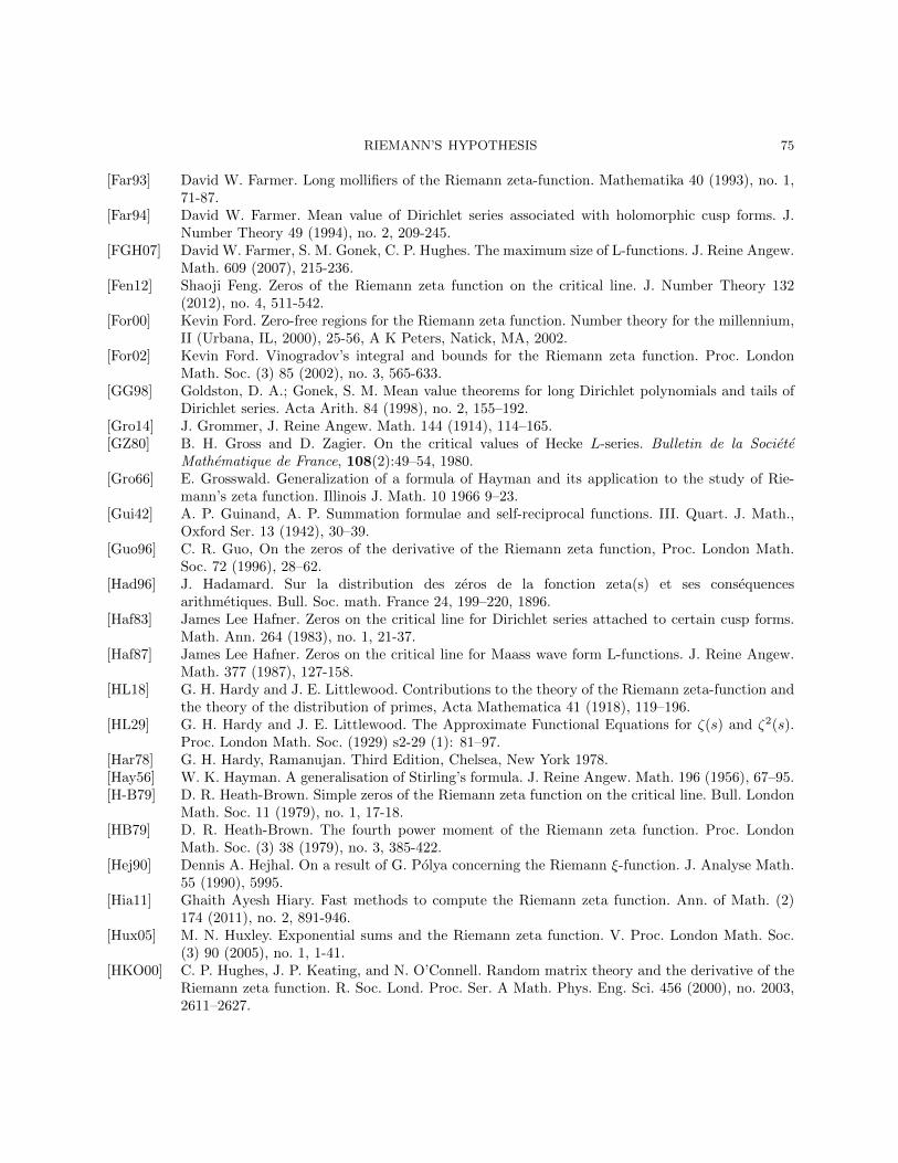
RIEMANN’S HYPOTHESIS 75
[Far93] David W. Farmer. Long mollifiers of the Riemann zeta-function. Mathematika 40 (1993), no. 1,71-87.
[Far94] David W. Farmer. Mean value of Dirichlet series associated with holomorphic cusp forms. J.Number Theory 49 (1994), no. 2, 209-245.
[FGH07] David W. Farmer, S. M. Gonek, C. P. Hughes. The maximum size of L-functions. J. Reine Angew.Math. 609 (2007), 215-236.
[Fen12] Shaoji Feng. Zeros of the Riemann zeta function on the critical line. J. Number Theory 132(2012), no. 4, 511-542.
[For00] Kevin Ford. Zero-free regions for the Riemann zeta function. Number theory for the millennium,II (Urbana, IL, 2000), 25-56, A K Peters, Natick, MA, 2002.
[For02] Kevin Ford. Vinogradov’s integral and bounds for the Riemann zeta function. Proc. LondonMath. Soc. (3) 85 (2002), no. 3, 565-633.
[GG98] Goldston, D. A.; Gonek, S. M. Mean value theorems for long Dirichlet polynomials and tails ofDirichlet series. Acta Arith. 84 (1998), no. 2, 155–192.
[Gro14] J. Grommer, J. Reine Angew. Math. 144 (1914), 114–165.[GZ80] B. H. Gross and D. Zagier. On the critical values of Hecke L-series. Bulletin de la Societe
Mathematique de France, 108(2):49–54, 1980.[Gro66] E. Grosswald. Generalization of a formula of Hayman and its application to the study of Rie-
mann’s zeta function. Illinois J. Math. 10 1966 9–23.[Gui42] A. P. Guinand, A. P. Summation formulae and self-reciprocal functions. III. Quart. J. Math.,
Oxford Ser. 13 (1942), 30–39.[Guo96] C. R. Guo, On the zeros of the derivative of the Riemann zeta function, Proc. London Math.
Soc. 72 (1996), 28–62.[Had96] J. Hadamard. Sur la distribution des zeros de la fonction zeta(s) et ses consequences
arithmetiques. Bull. Soc. math. France 24, 199–220, 1896.[Haf83] James Lee Hafner. Zeros on the critical line for Dirichlet series attached to certain cusp forms.
Math. Ann. 264 (1983), no. 1, 21-37.[Haf87] James Lee Hafner. Zeros on the critical line for Maass wave form L-functions. J. Reine Angew.
Math. 377 (1987), 127-158.[HL18] G. H. Hardy and J. E. Littlewood. Contributions to the theory of the Riemann zeta-function and
the theory of the distribution of primes, Acta Mathematica 41 (1918), 119–196.[HL29] G. H. Hardy and J. E. Littlewood. The Approximate Functional Equations for ζ(s) and ζ2(s).
Proc. London Math. Soc. (1929) s2-29 (1): 81–97.[Har78] G. H. Hardy, Ramanujan. Third Edition, Chelsea, New York 1978.[Hay56] W. K. Hayman. A generalisation of Stirling’s formula. J. Reine Angew. Math. 196 (1956), 67–95.[H-B79] D. R. Heath-Brown. Simple zeros of the Riemann zeta function on the critical line. Bull. London
Math. Soc. 11 (1979), no. 1, 17-18.[HB79] D. R. Heath-Brown. The fourth power moment of the Riemann zeta function. Proc. London
Math. Soc. (3) 38 (1979), no. 3, 385-422.[Hej90] Dennis A. Hejhal. On a result of G. Polya concerning the Riemann ξ-function. J. Analyse Math.
55 (1990), 5995.[Hia11] Ghaith Ayesh Hiary. Fast methods to compute the Riemann zeta function. Ann. of Math. (2)
174 (2011), no. 2, 891-946.[Hux05] M. N. Huxley. Exponential sums and the Riemann zeta function. V. Proc. London Math. Soc.
(3) 90 (2005), no. 1, 1-41.[HKO00] C. P. Hughes, J. P. Keating, and N. O’Connell. Random matrix theory and the derivative of the
Riemann zeta function. R. Soc. Lond. Proc. Ser. A Math. Phys. Eng. Sci. 456 (2000), no. 2003,2611–2627.
76 BRIAN CONREY
[Ing90] A. E. Ingham. The distribution of prime numbers. Reprint of the 1932 original. With a forewordby R. C. Vaughan. Cambridge Mathematical Library. Cambridge University Press, Cambridge,1990.
[Ing40] A. E. Ingham. On the estimation of N(s,T). Quart. J. Math., Oxford Ser. 11, (1940). 291-292.[IK04] Henryk Iwaniec, Emmanuel Kowalski. Analytic number theory. American Mathematical Society
Colloquium Publications, 53. American Mathematical Society, Providence, RI, 2004.[JMMS80] Michio Jimbo, Tetsuji Miwa, Yasuko Mori, Mikio Sato. Density matrix of an impenetrable Bose
gas and the fifth Painlev transcendent. Phys. D 1 (1980), no. 1, 80-158.[KP99] J. Kaczorowski, A. Perelli. The Selberg class: a survey. Number theory in progress, Vol. 2
(Zakopane-Koscielisko, 1997), 953–992, de Gruyter, Berlin, 1999.[Kar68] Samuel Karlin. Total positivity. Vol. I. Stanford University Press, Stanford, Calif 1968 xii+576
pp.[KatS93] Svetlana Katok, Peter Sarnak. Heegner points, cycles and Maass forms. Israel J. Math. 84 (1993),
no. 1-2, 193-227.[KaSa99] Nicholas M. Katz, Peter Sarnak. Zeroes of zeta functions and symmetry. Bull. Amer. Math. Soc.
(N.S.) 36 (1999), no. 1, 1-26.[KS00] J. P. Keating, N. C. Snaith. Random matrix theory and ζ(1/2 + it). Commun. Math. Phys. 214
(2000), no. 1, 57–89.[Ki05] Haseo Ki. All but finitely many non-trivial zeros of the approximations of the Epstein zeta
function are simple and on the critical line. Proc. London Math. Soc. (3) 90 (2005), no. 2,321-344.
[KK02] Haseo Ki, Young-One Kim. A generalization of Newman’s result on the zeros of Fourier trans-forms. Comput. Methods Funct. Theory 2 (2002), no. 2, 449–467.
[KK03] Haseo Ki, Young-One Kim. de Bruijn’s question on the zeros of Fourier transforms. J. Anal.Math. 91 (2003), 369–387.
[KZ81] W. Kohnen, D. Zagier. Values of L-series of modular forms at the center of the critical strip.Invent. Math. 64 (1981), no. 2, 175-198.
[Kor58] N. M. Korobov. Estimates of trigonometric sums and their applications. (Russian) Uspehi Mat.Nauk 13 1958 no. 4 (82), 185-192.
[KMV00] E. Kowalski, P. Michel, J. VanderKam. Mollification of the fourth moment of automorphic L-functions and arithmetic applications. Invent. Math. 142 (2000), no. 1, 95-151.
[Lac04] Gilles Lachaud. Spectral analysis and the Riemann hypothesis. Proceedings of the InternationalConference on Special Functions and their Applications (Chennai, 2002). J. Comput. Appl. Math.160 (2003), no. 1-2, 175-190.
[Lag06] J. Lagarias. Hilbert spaces of entire functions and Dirichlet L-functions. Frontiers in numbertheory, physics, and geometry. I, 365377, Springer, Berlin, 2006.
[LY52] T. D. Lee, C. N. Yang. Statistical theory of equations of state and phase transitions. II. Latticegas and Ising model. Physical Rev. (2) 87, (1952). 410-419.
[Lev74] Norman Levinson. More than one third of zeros of Riemann’s zeta-function are on s=1/2. Ad-vances in Math. 13 (1974), 383-436.
[LM74] Norman Levinson, Hugh L. Montgomery. Zeros of the derivatives of the Riemann zeta-function.Acta Math. 133 (1974), 49–65.
[LMFDB] The L-functions and modular forms database. http://www.lmfdb.org/[Li97] Xian-Jin Li. The positivity of a sequence of numbers and the Riemann hypothesis. J. Number
Theory 65 (1997), no. 2, 325–333.[LS81] Elliott H. Lieb, Alan D. Sokal. A general Lee-Yang theorem for one-component and multicom-
ponent ferromagnets. Comm. Math. Phys. 80 (1981), no. 2, 153-179.

RIEMANN’S HYPOTHESIS 77
[Low68] M. Low. Real zeros of the Dedekind zeta function of an imaginary quadratic field. Acta Arith.14 (1968), 117–140.
[Mas06] Krzysztof Maslanka. Bez-Duarte’s Criterion for the Riemann Hypothesis and Rice’s Integrals.arxiv math.NT/0603713.
[MSS14] Adam Marcus, Daniel A Spielman, Nikhil Srivastava. Interlacing Families II: Mixed Character-istic Polynomials and the Kadison-Singer Problem. arXiv:1306.3969.
[Mat82] Yu V. Matiyasevich, Yet another machine experiment in support of Riemann’s conjecture. Cy-bernetics 18 (1982) 705.
[Meh04] Madan Lal Mehta. Random matrices. Third edition. Pure and Applied Mathematics (Amster-dam), 142. Elsevier/Academic Press, Amsterdam, 2004. xviii+688 pp.
[Mey04] R. Meyer. A spectral interpretation for the zeros of the Riemann zeta function.arXiv:math/0412277v3
[Mez03] Francesco Mezzadri. Random matrix theory and the zeros of ζ ′(s). Random matrix theory. J.Phys. A 36 (2003), no. 12, 2945–2962.
[Mon73] H.L. Montgomery. The pair correlation of zeros of the zeta function. Analytic number theory,Proc. Sympos. Pure Math., Vol. XXIV, St. Louis Univ., St. Louis, Mo., 1972, pp. 181-193. Amer.Math. Soc., Providence, R.I., 1973.
[Mot97] Yichi Motohashi. Spectral theory of the Riemann zeta-function. Cambridge Tracts in Mathemat-ics, 127. Cambridge University Press, Cambridge, 1997. x+228 pp.
[New76] CharlesM. Newman. Fourier transforms with only real zeros. Proc. Amer. Math. Soc. 61 (1976),no. 2, 245–251 (1977).
[New91] Charles M. Newman, Charles M. The GHS inequality and the Riemann hypothesis. Constr.Approx. 7 (1991), no. 3, 389–399.
[Nut13] John Nuttall. Wronskians, cumulants, and the Riemann hypothesis. Constr. Approx. 38 (2013),no. 2, 193-212
[Nym50] B. Nyman, On the one-dimensional translation group and semi-group in certain function spaces,PhD thesis, Uppsala, 1950.
[Odl00] A. M. Odlyzko. An improved bound for the de Bruijn-Newman constant. Mathematical journeythrough analysis, matrix theory and scientific computation (Kent, OH, 1999). Numer. Algorithms25 (2000), no. 1–4, 293–303.
[OS88] A. M. Odlyzko, A. Schonhage,. Fast algorithms for multiple evaluations of the Riemann zetafunction. Trans. Amer. Math. Soc. 309 (1988), no. 2, 797-809.
[Pat88] S. J. Patterson. An introduction to the theory of the Riemann zeta-function. Cambridge Studiesin Advanced Mathematics, 14. Cambridge University Press, Cambridge, 1988.
[Pla13] David J. Platt. Numerical Computations Concerning the GRH. arXiv:1305.3087.
[Pol26] G. Polya, G. Bemerkung Uber die Integraldarstellung der Riemannschen ξ-Funktion. Acta Math.48 (1926), no. 3–4, 305-317.
[Pol27] G. Polya, Uber trigonometrische Integrale mit nur reellen Nullstellen. J. Reine Angew. Math.158 (1927) 6–18.
[Pol27b] G. Polya. Uber die algebraisch-funktiontheoretischen Untersuchungen von J. L. W. V. Jensen.Kgl. Danske Vid. Sel. Math.-Fys. Medd. 7 (17) (1927).
[PS98] George Polya, Gabor Szego. Problems and theorems in analysis. II. Theory of functions, zeros,polynomials, determinants, number theory, geometry. Translated from the German by C. E.Billigheimer. Reprint of the 1976 English translation. Classics in Mathematics. Springer-Verlag,Berlin, 1998. xii+392 pp.
[Ric67] H.-E. Richert. Zur Abschtzung der Riemannschen Zetafunktion in der Nhe der Vertikalen s=1.Math. Ann. 169 (1967) 97-101.
78 BRIAN CONREY
[R] Bernhard Riemann. Ueber die Anzahl der Primzahlen unter einer gegebenen Grosse. Monats-berichte der Berliner Akademie, November 1859.
[Rie16] M. Riesz, Sur lhypoth‘ese de Riemann, Acta Math. 40, 185–190 (1916).[RVZ93] F. Rodriguez-Villegas and D. Zagier. Square roots of central values of Hecke L -series. In Advances
in number theory (Kingston, ON, 1991), 81–99. Oxford Sci. Publ., Oxford Univ. Press, New York,1993.
[Roe86] Friedrich Roesler. Riemann’s hypothesis as an eigenvalue problem. Linear Algebra Appl. 81(1986), 153–198.
[Roe87] Roesler, Friedrich. Riemann’s hypothesis as an eigenvalue problem. II. Linear Algebra Appl. 92(1987), 45–73.
[Ros02] Rosen, Michael Number theory in function fields. Graduate Texts in Mathematics, 210. Springer-Verlag, New York, 2002.
[Rub13] Michael O. Rubinstein. Elliptic curves of high rank and the Riemann zeta function on the oneline. Exp. Math. 22 (2013), no. 4, 465-480.
[Rue88] Ruelle, David Is our mathematics natural? The case of equilibrium statistical mechanics. Bull.Amer. Math. Soc. (N.S.) 19 (1988), no. 1, 259-268.
[Sal52] R. Salem. Uniform distribution and capacity of sets. Comm. Sm. Math. Univ. Lund [Medd. LundsUniv. Mat. Sem.] 1952, (1952). Tome Supplementaire, 193–195.
[Sch73] Wolfgang M. Schmidt. Zur Methode von Stepanov. Collection of articles dedicated to Carl LudwigSiegel on the occasion of his seventy-fifth birthday, IV. Acta Arith. 24 (1973), 347–367.
[Sel42] Atle Selberg. On the zeros of Riemann’s zeta-function. Skr. Norske Vid. Akad. Oslo I. 1942,(1942). no. 10, 59 pp.
[Sel89] Atle Selberg. Old and new conjectures and results about a class of Dirichlet series. Proceedingsof the Amalfi Conference on Analytic Number Theory (Maiori, 1989), 367–385, Univ. Salerno,Salerno, 1992.
[Sie32] C. L. Siegel. Uber Riemann’s Nachlaß zur analytischen Zahlentheorie. Quellen Studien zurGeschichte der Math. Astron. und Phys. Abt. B: Studien 2, 45–80, 1932. Reprinted in GesammelteAbhandlungen, Vol. 1. Berlin: Springer-Verlag, 1966.
[Sou98] K. Soundararajan. The horizontal distribution of zeros of ζ ′(s). Duke Math. J. 91 (1998), no. 1,33–59.
[Sou00] K. Soundararajan. Nonvanishing of quadratic Dirichlet L-functions at s=12. Ann. of Math. (2)152 (2000), no. 2, 447-488.
[Sou08] K. Soundararajan. Extreme values of zeta and L-functions. Math. Ann. 342 (2008), no. 2, 467-486.[Spe35] Andreas Speiser. Geometrisches zur Riemannschen Zetafunktion. Math. Ann. 110 (1935), no. 1,
514–521.[Ste69] S. A. Stepanov. The number of points of a hyperelliptic curve over a finite prime field. (Russian)
Izv. Akad. Nauk SSSR Ser. Mat. 33 1969 1171–1181.[Tit86] E. C. Titchmarsh. The theory of the Riemann zeta-function. Second edition. Edited and with a
preface by D. R. Heath-Brown. The Clarendon Press, Oxford University Press, New York, 1986.x+412 pp.
[Tur53] A. M. Turing. Some calculations of the Riemann zeta-function. Proc. London Math. Soc. (3) 3,(1953). 99-117.
[Val96] C.-J. de la Vallee Poussin. Recherches analytiques la theorie des nombres premiers. Ann. Soc.scient. Bruxelles 20, 183–256, 1896.
[Vas95] V. I. Vasyunin. On a biorthogonal system associated with the Riemann hypothesis. (Russian)Algebra i Analiz 7 (1995), no. 3, 118–135; translation in St. Petersburg Math. J. 7 (1996), no. 3,405–419.

RIEMANN’S HYPOTHESIS 79
[Vas99] V. I. Vasyunin, V. I. On a system of step functions. (Russian) Zap. Nauchn. Sem. S.-Peterburg.Otdel. Mat. Inst. Steklov. (POMI) 262 (1999), Issled. po Linein. Oper. i Teor. Funkts. 27, 49–70,231–232; translation in J. Math. Sci. (New York) 110 (2002), no. 5, 2930–2943
[Vau93] R. C. Vaughan. On the eigenvalues of Redheffer’s matrix. I. Number theory with an emphasison the Markoff spectrum (Provo, UT, 1991), 283–296, Lecture Notes in Pure and Appl. Math.,147, Dekker, New York, 1993.
[Vau96] R. C. Vaughan. On the eigenvalues of Redheffer’s matrix. II. J. Austral. Math. Soc. Ser. A 60(1996), no. 2, 260–273.
[Vin58] I. M. Vinogradov. A new estimate of the function ζ(1 + it). (Russian) Izv. Akad. Nauk SSSR.Ser. Mat. 22 1958 161-164.
[Wal81] Waldspurger, J.-L. Sur les coefficients de Fourier des formes modulaires de poids demi-entier. J.Math. Pures Appl. (9) 60 (1981), no. 4, 375-484.
[Wat02] Mark Watkins. Notes on Connes and RH. http://magma.maths.usyd.edu.au/users/watkins/papers/connes.pdf[Wat04] M. Watkins. Real zeros of real odd Dirichlet L-functions, Math. Comp. 73 (2004), 415-423.[Wei52] A. Weil. Sur les “formules explicites” de la thorie des nombres premiers. Comm. Sem. Math.
Univ. Lund [Medd. Lunds Univ. Mat. Sem.] 1952 (1952), Tome Supplementaire, 252–265.[Wie32] N. Wiener. Tauberian theorems, Ann. of Math. 33 (1932), 1–100.[Wol06] M. Wolf. Evidence in favor of the Baez-Duarte criterion for the Riemann hypothesis,
math.NT/0605485 (2006).[Yos90] H. Yoshida. On Hermitian forms attached to zeta functions. Zeta functions in geometry (Tokyo,
1990), 281–325. Advanced Studies in Pure Mathematics, 21. Kinokuniya, Tokyo, 1992.[Zha01] Yitang Zhang. On the zeros of ζ ′(s) near the critical line. Duke Math. J. 110 (2001), no. 3,
555–572.
American Institute of Mathematics, 360 Portage Ave, Palo Alto, CA 94306, USA andSchool of Mathematics, University of Bristol, Bristol BS8 1TW, UK
E-mail address: [email protected]