richard m. yablonsky university of rhode island wrf for · pdf filerichard m. yablonsky...

1

Richard M. YablonskyUniversity of Rhode Island

WRF for Hurricanes TutorialBoulder, CO28 April 2011

2

What is the Princeton Ocean Model?

Three-dimensional, primitive equation, numerical ocean model (commonly known as POM)

Originally developed by Alan Blumberg and George Mellor in the late 1970’s

Initially used for coastal ocean circulation applications (Blumberg and Mellor 1987)

Open to the community during the 1990’s and 2000’s

Many user-generated changes incorporated into “official” code version housed at Princeton University

3

Developing HWRF Ocean (POM-TC)

Available POM code version transferred to University of Rhode Island (URI) in mid-1990’s

POM code changes made at URI specifically to address ocean response to hurricane wind forcing

This POM version coupled to GFDL hurricane model at URI

Coupled GFDL/POM model operational at NCEP in 2001

Additional POM upgrades made at URI during 2000’s (e.g. initialization) and implemented in operational GFDL/POM

Same version of POM coupled to operational HWRF in 2007

This POM version henceforth designated “POM-TC”

Some further POM-TC upgrades made at URI since 2007

4

Why Couple POM-TC to HWRF?

To create accurate SST field for input into the HWRF

Evaporation (moisture flux) from sea surface provides heat energy to drive a hurricane

Available energy decreases if storm-core SST decreases

Uncoupled hurricane models with static SST neglect SST cooling during integration high intensity bias

One-dimensional (vertical-only) ocean models neglect upwelling, which can impact SST during integration (e.g. Yablonsky and Ginis 2009, MWR)

6

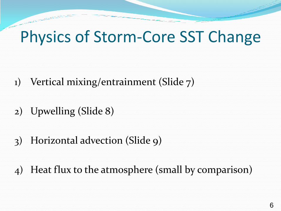
Physics of Storm-Core SST Change

1) Vertical mixing/entrainment (Slide 7)

2) Upwelling (Slide 8)

3) Horizontal advection (Slide 9)

4) Heat flux to the atmosphere (small by comparison)

7

A

T

M

O

S

P

H

E

R

E

O

C

E

A

N

Warm sea surface temperature

Cool subsurface temperature

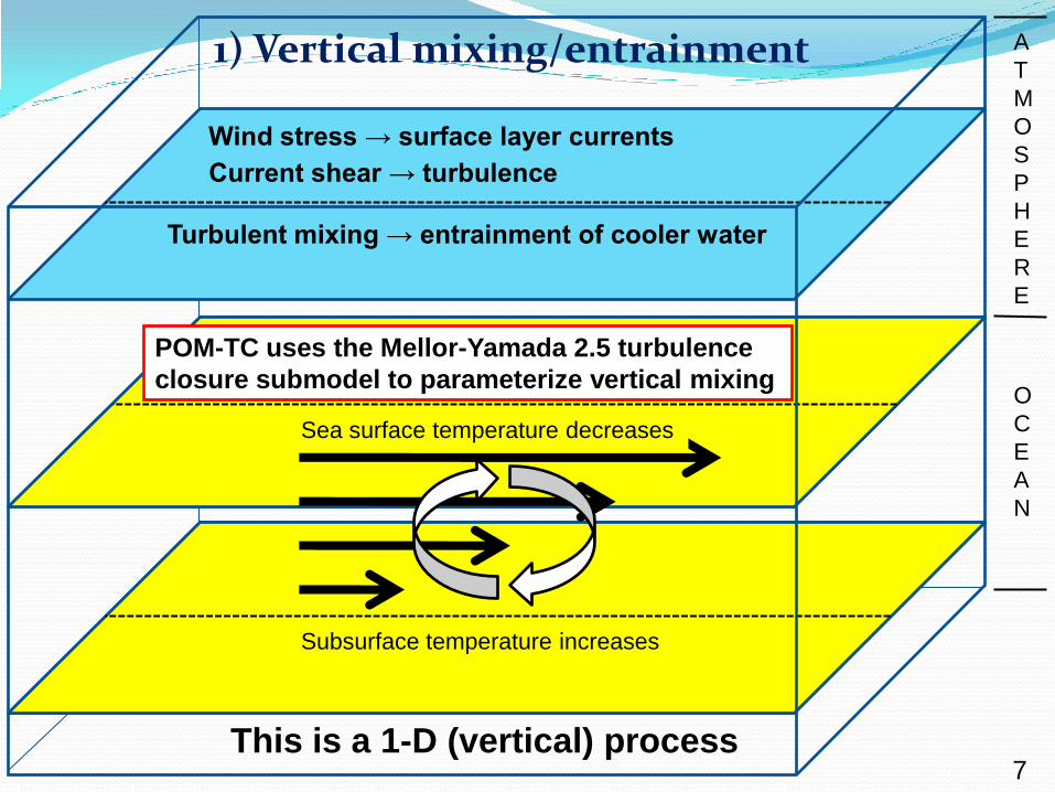
1) Vertical mixing/entrainment

Wind stress → surface layer currents

Current shear → turbulence

Turbulent mixing → entrainment of cooler water

Sea surface temperature decreases

Subsurface temperature increases

This is a 1-D (vertical) process

POM-TC uses the Mellor-Yamada 2.5 turbulence

closure submodel to parameterize vertical mixing

8

Cyclonic

hurricane

vortex

A

T

M

O

S

P

H

E

R

E

O

C

E

A

N



2) Upwelling

Cyclonic wind stress → divergent surface currents

Divergent currents → upwelling

Upwelling → cooler water brought to surface

This is a 3-D process

9

Cyclonic

hurricane

vortex

A

T

M

O

S

P

H

E

R

E

O

C

E

A

N



3) Horizontal advection

Preexisting cold pool is located outside storm core

Preexisting current direction is towards storm core

Ocean currents advect cold pool under storm core

This is a horizontal process

10

Prescribed propagation speed

Cyclonic

hurricane

vortex

A

T

M

O

S

P

H

E

R

E

O

C

E

A

N

Homogeneous initial SST

Horizontally-homogeneous subsurface temperature

What is the impact of varying storm translation speed?

<

<

<

<

<

<

<

<

<

<

<

<

11

2.4 m s-1 4.8 m s-1

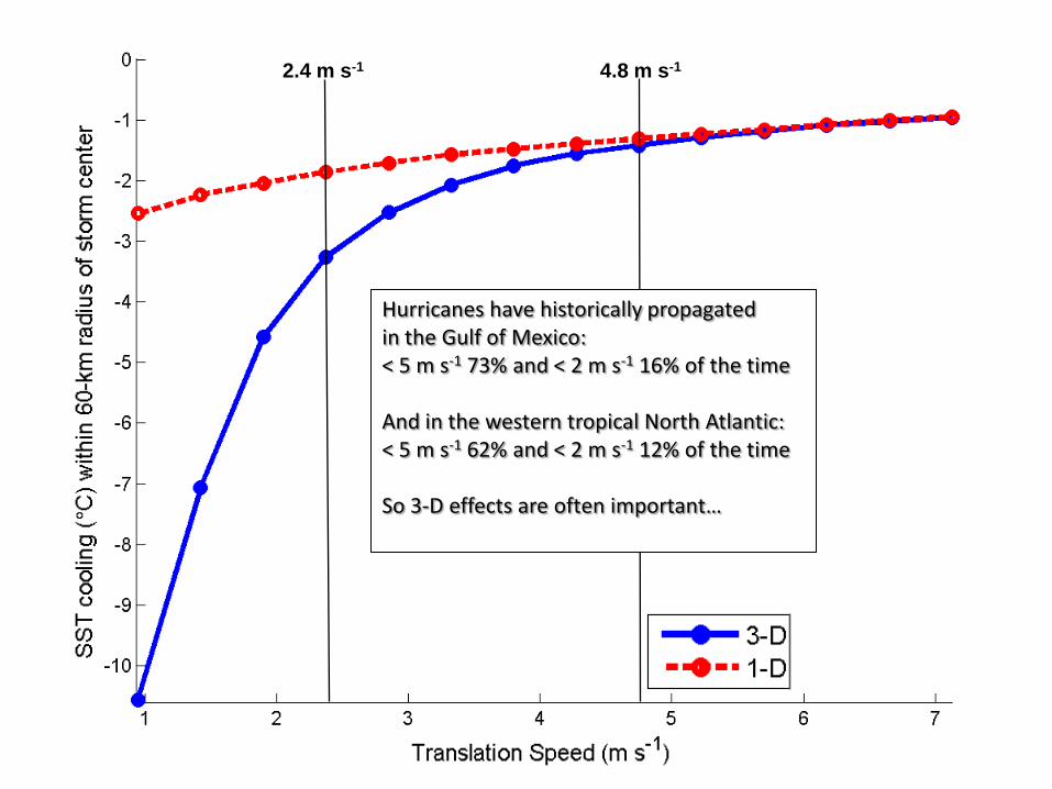
Hurricanes have historically propagatedin the Gulf of Mexico:< 5 m s-1 73% and < 2 m s-1 16% of the time

And in the western tropical North Atlantic:< 5 m s-1 62% and < 2 m s-1 12% of the time

So 3-D effects are often important…

1-D3-D

2.4 m s-1

1-D

4.8 m s-1

3-D

13

POM-TC Grid: “United” Region

225

254

47.5 N

10 N

50 W98.5 W

~18-km grid spacing

14

POM-TC Grid: “East Atlantic” Region

225

209

47.5 N

10 N

30 W~70 W

~18-km grid spacing

2011 Operational HWRF:

Western edge = 60 W

15

POM-TC Sigma Vertical Coordinate

• 23 vertical sigma levels; free surface (η)

• Level placement scaled based on ocean bathymetry

• Largest vertical spacing occurs where ocean depth is 5500 m

• Location of 23 half-sigma levels when ocean depth is 5500 m:

5, 15, 25, 35, 45, 55, 65, 77.5, 92.5, 110, 135, 175, 250, 375,

550, 775, 1100, 1550, 2100, 2800, 3700, 4850, and 5500 m

16

• Horizontal spatial differencing occurs on staggered Arakawa-C grid

• 2-D variables “UA” and “VA” are calculated at shifted location from “η”

Arakawa-C Grid: External Mode

Plan View

17

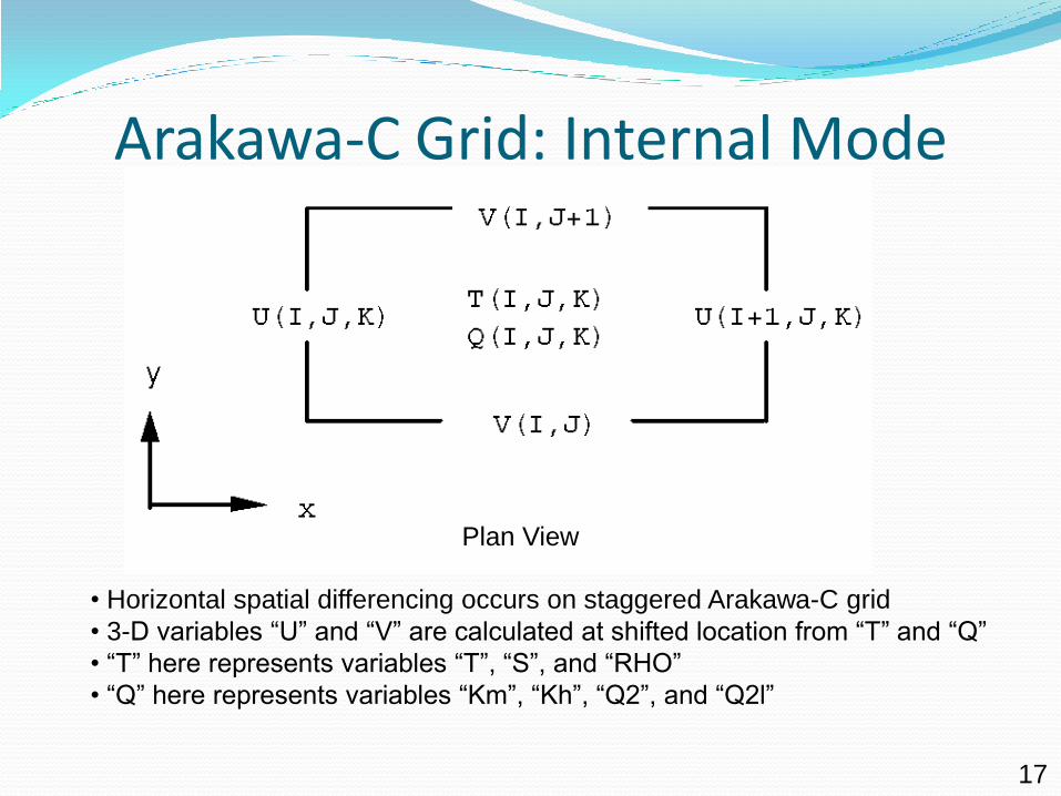
• Horizontal spatial differencing occurs on staggered Arakawa-C grid

• 3-D variables “U” and “V” are calculated at shifted location from “T” and “Q”

• “T” here represents variables “T”, “S”, and “RHO”

• “Q” here represents variables “Km”, “Kh”, “Q2”, and “Q2l”

Arakawa-C Grid: Internal Mode

Plan View

18

• Vertical spatial differencing also occurs on staggered grid

• 3-D variables “W” and “Q” are calculated at shifted depth from “T” and “U”

• “T” here represents variables “T”, “S”, and “RHO”

• “Q” here represents variables “Km”, “Kh”, “Q2”, and “Q2l”

Vertical Grid: Internal Mode

Elevation View

19

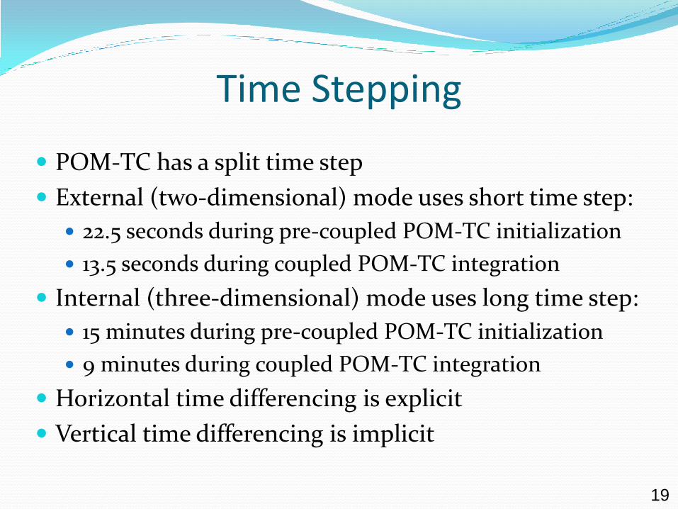
POM-TC has a split time step

External (two-dimensional) mode uses short time step:

22.5 seconds during pre-coupled POM-TC initialization

13.5 seconds during coupled POM-TC integration

Internal (three-dimensional) mode uses long time step:

15 minutes during pre-coupled POM-TC initialization

9 minutes during coupled POM-TC integration

Horizontal time differencing is explicit

Vertical time differencing is implicit

Time Stepping

20

Prior to coupled model integration of HWRF/POM-TC, POM-TC must be initialized with a realistic, 3-D temperature (T) and salinity (S) field

This T & S field must then be used to generate realistic ocean currents via geostrophic adjustment

The “spun-up” ocean must then incorporate the preexisting hurricane-generated cold wake by applying TC’s wind stress using the NHC hurricane message file

POM-TC initialization

21

Typical of

Gulf of Mexico in

Summer & Fall Typical of

Caribbean in

Summer & Fall

22

Subsurface (75-m)

ocean temperature

during Katrina & Rita

Warm Loop Current

water and a warm

core ring extend far

into the Gulf of Mexico

from the Caribbean…

Directly under Rita’s

& Katrina’s track…

But… how do we know

the locations of (& how

do we assimilate) these

features in real-time?

Approximate Locations of Oceanic Features

During Hurricanes Katrina and Rita (2005)

Rita Katrina

TX LA

MS AL GA

FL

Mexico

Gulf of Mexico

C

Caribbean

Loop Current

warm

core ring

cold

core ring

23

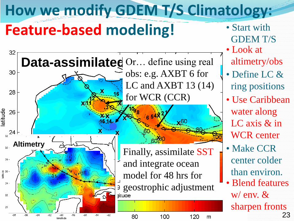
GDEMData-assimilated

How we modify GDEM T/S Climatology:Feature-based modeling!

• Look at

altimetry/obs

• Define LC &

ring positions

• Use Caribbean

water along

LC axis & in

WCR center

• Make CCR

center colder

than environ.• Blend features

w/ env. &

sharpen fronts

Altimetryx

x

xx

x

x x

x

x

x x

x

xx

x

• Start with

GDEM T/S

Or… define using real

obs: e.g. AXBT 6 for

LC and AXBT 13 (14)

for WCR (CCR)

Finally, assimilate SST

and integrate ocean

model for 48 hrs for

geostrophic adjustment

24

Gustav 2008082800:Ocean Initialization & Response

(Next 6 Slides)

25

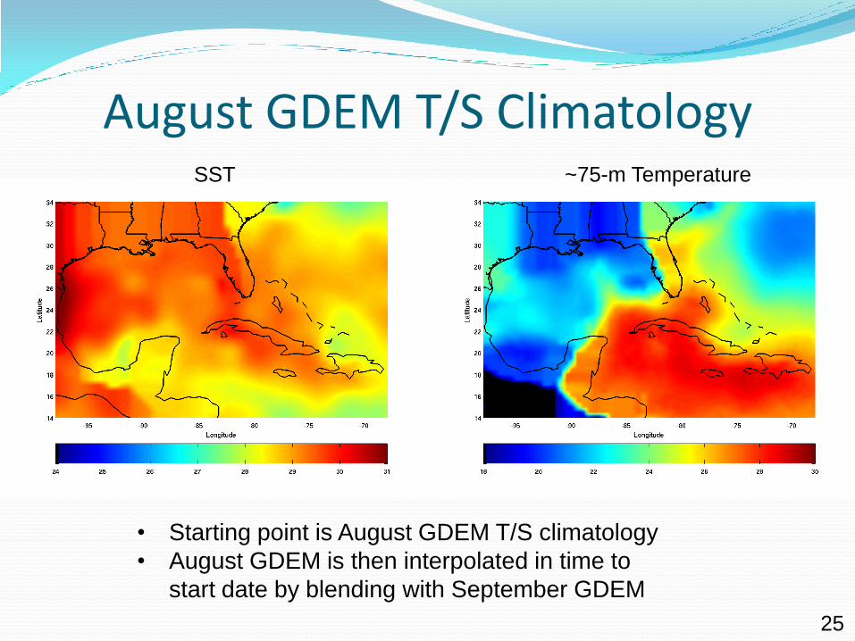
August GDEM T/S ClimatologySST ~75-m Temperature

• Starting point is August GDEM T/S climatology

• August GDEM is then interpolated in time to

start date by blending with September GDEM

26

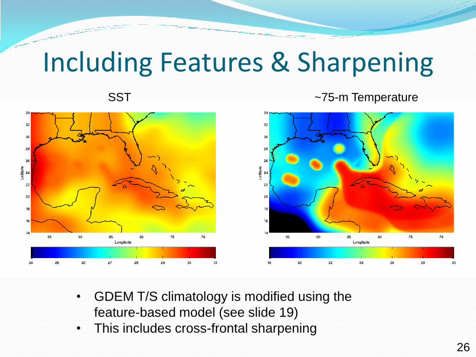
Including Features & SharpeningSST ~75-m Temperature

• GDEM T/S climatology is modified using the

feature-based model (see slide 19)

• This includes cross-frontal sharpening

27

00-hr Phase 1: GFS SST AssimilatedSST ~75-m Temperature

• At 00-hr phase 1, daily NCEP SST is assimilated

into the upper ocean mixed layer

• T/S fields vertically-interpolated to POM σ-levels

(Land/sea mask applied)

28

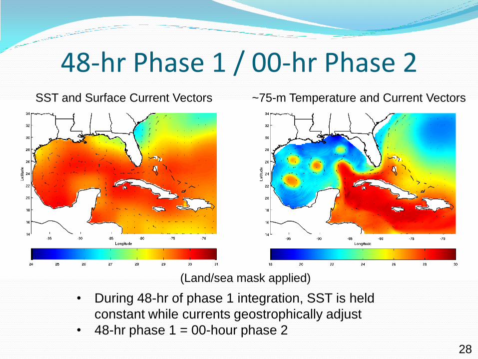
48-hr Phase 1 / 00-hr Phase 2SST and Surface Current Vectors ~75-m Temperature and Current Vectors


• During 48-hr of phase 1 integration, SST is held

constant while currents geostrophically adjust

• 48-hr phase 1 = 00-hour phase 2

29

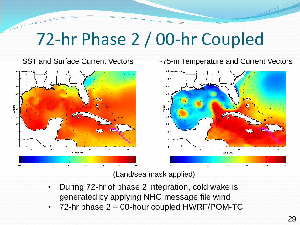
72-hr Phase 2 / 00-hr CoupledSST and Surface Current Vectors ~75-m Temperature and Current Vectors


• During 72-hr of phase 2 integration, cold wake is

generated by applying NHC message file wind

• 72-hr phase 2 = 00-hour coupled HWRF/POM-TC

30

192-hr Phase 2 (like 120-hr Coupled)SST and Surface Current Vectors ~75-m Temperature and Current Vectors


• During 120-hr of coupled HWRF/POM-TC run, cold

wake is generated by HWRF wind + thermal forcing

• Cold wake is generated here by extending phase 2

31

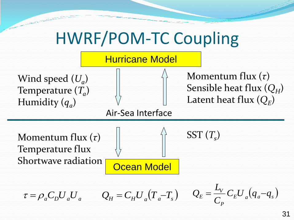
Hurricane Model

Ocean Model

Air-Sea Interface

aaDa UUC saaHH TTUCQ saaE

P

VE qqUC

C

LQ

Momentum flux (τ)Sensible heat flux (QH)Latent heat flux (QE)

SST (Ts)

Wind speed (Ua)Temperature (Ta)Humidity (qa)

Momentum flux (τ)Temperature fluxShortwave radiation

HWRF/POM-TC Coupling

32

How to Run the POM-TC Ocean Initialization: Technical Details

(Next 13 Slides)

33

Scripts can be found in directory: ${HOME}/HWRF/src/pomtc/ocean_scripts

There are 6 scripts, 5 of which are “kickit” scripts

Sixth script “gfdl_pre_ocean_sortvit.sh” is used internally by a “kickit” script and should not be changed

Five “kickit” scripts are designed to be run in order from kickit00 through kickit04

If running default tutorial case 2008082800 on Bluefire, no changes should be needed to the kickit scripts

Next slide explains how to run ocean initialization

Scripts

34

Go to the following directory: ${HOME}/HWRF/src/pomtc/ocean_scripts

Execute the five kickit scripts sequentially:[prompt]$ ./kickit00_region.sh

[prompt]$ ./kickit01_sharpn.sh

[prompt]$ ./kickit02_getsst.sh

[prompt]$ ./kickit03_phase3.sh

[prompt]$ ./kickit04_phase4.sh

Next slide explains how to modify the “kickit” scripts if running a case other than default case 2008082800

Running the Ocean Initialization

35

If running a case other than 2008082800, edit the five “kickit” scripts before running them

If running on Bluefire, the only two lines in each “kickit” script that need to be edited are:stormid=07L # e.g. SID = 07L

start_date=2008082800 # e.g. YYYYMMDDHH = 2008082800

If running on a machine other than Bluefire, these lines may also need to be edited, depending on the paths to your input datasets, source code, and output directories:data_d=/ptmp/HurrTutorial/datasets

sorc_d=${HOME}/HWRF/src/pomtc

work_d=/ptmp/${USER}/HWRF/${stormid}/${start_date}/oceanprd

Modifying the “kickit” Scripts

36

Set the storm ID

Set the starting date for POM-TC as YYYYMMDDHH

Define the directories

Set up paths to certain shell commands

Create the work directory if it does not already exist

Slice up the starting date

Use a piece of the storm ID to determine the ocean basin

Continue with the following steps if region is Atlantic; otherwise, run uncoupled

Run operational script gfdl_pre_ocean_sortvit.sh to extract track information for the specified storm from the yearly NHC hurricane message file (i.e. TC Vitals). Then, append a line of zeros at the end of this complete track file

Use an embedded Perl script to remove all cycles after the current one from the complete track file and save as a shortened track file

Use the shortened track file for subsequent steps unless it is empty

Procedures in kickit00_region.sh

37

Extract various storm statistics from the track file and use those statistics to generate a 72-hour projected track that assumes storm direction and speed remain constant. Save this projected track in a “shortstats” file

Run the find region code, which selects the ocean region based on the projected track points in the “shortstats” file

Write region info to “pom_region.txt” in preparation for POM-TC phase 3

End the region selection script by returning to the “ocean_scripts” directory

Procedures in kickit00_region.sh (continued)

38

Set the storm ID

Set starting date for POM-TC as YYYYMMDDHH

Set which ocean climatology to use (default is GDEM)

Set the ocean region. If ocean region is not “united,” skip the following steps



Create the sharpening directory, overwriting old attempts

Slice up the storm ID and starting date

If Loop Current files are missing, use climate LC penetration instead

Use some pieces of starting date to select two climatology months

Create parameter “input_sharp” depending on chosen climatology

Create symbolic links for the input files

Run the sharpening code

Rename the sharpened climatology file in preparation for POM-TC phase 3

End the sharpening script by returning to the “ocean_scripts” directory

Procedures in kickit01_sharpn.sh

39

Set the storm ID




Create the sst/mask/lonlat directory, overwriting old attempts

Slice up the starting date, using HH to define the model cycle

Create symbolic links for the GFS spectral input files

Increase ulimit –s to prevent a segmentation fault

Run the getsst code

Rename the sst/mask/lonlat files in preparation for POM-TC phase 3

End the getsst script by returning to the “ocean_scripts” directory

Procedures in kickit02_getsst.sh

40

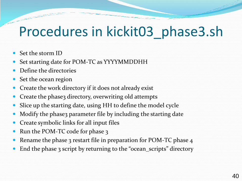
Set the storm ID



Set the ocean region


Create the phase3 directory, overwriting old attempts


Modify the phase3 parameter file by including the starting date

Create symbolic links for all input files

Run the POM-TC code for phase 3

Rename the phase 3 restart file in preparation for POM-TC phase 4

End the phase 3 script by returning to the “ocean_scripts” directory

Procedures in kickit03_phase3.sh

41

Set the storm ID



Set the ocean region


Create the phase 4 directory, overwriting old attempts

If track file created in kickit00_region.sh is less than three lines, skip the steps below and use the phase 3 restart file to initialize the coupled HWRF run


Use the GNU date command to start phase 4 three days prior to coupled forecast

Copy track file to the phase 4 directory, and modify the phase 4 parameter file by including the starting date, as well as the track and phase 3 restart files

Create symbolic links for all input files

Run the POM-TC code for phase 4

Rename the phase4 restart file in preparation for coupled HWRF run

End the phase 4 script by returning to the “ocean_scripts” directory

Procedures in kickit04_phase4.sh

42

There are 5 executable files associated with POM-TC ocean initialization, which can be found in directory: ${HOME}/HWRF/src/pomtc/ocean_exec

The following slides list the function, input(s), output(s), and usage of each of these 5 executable files

Executables

43

Function: Determine which POM-TC region to use based on the current and projected storm track given in the “shortstats” file

Input(s): shortstats

Output(s): fort.61 (ocean_region_info.txt)

Usage: ${HOME}/HWRF/src/pomtc/ocean_exec/gfdl_find_region.exe < shortstats

gfdl_find_region.exe

44

Function: Extract SST, land-sea mask, and lon/lat data from the GFS spectral files

Input(s): for11 (gfs.${start_date}.t${cyc}z.sfcanl)

fort.11 (gfs.${start_date}.t${cyc}z.sfcanl)

fort.12 (gfs.${start_date}.t${cyc}z.sanl)

Output(s): fort.23 (lonlat.gfs)

fort.74 (sst.gfs.dat)

fort.77 (mask.gfs.dat)

getsst.out

Usage: ${HOME}/HWRF/src/pomtc/ocean_exec/gfdl_getsst.exe >> getsst.out

gfdl_getsst.exe

45

Function: Run the sharpening program, which takes the T/S climatology, horizontally-interpolates it onto the POM-TC grid for the United region domain, assimilates a land/sea mask and bathymetry, and employs the diagnostic, feature-based modeling procedure

Input(s): input_sharp

fort.66 (gfdl_ocean_topo_and_mask.${region})

fort.8 (gfdl_gdem.${mm}.ascii)

fort.90 (gfdl_gdem.${mmm2}.ascii)

fort.24 (gfdl_ocean_readu.dat.${mm})

fort.82 (gfdl_ocean_spinup_gdem3.dat.${mm})

fort.50 (gfdl_ocean_spinup_gspath.${mm})

fort.55 (gfdl_ocean_spinup.BAYuf)

fort.65 (gfdl_ocean_spinup.FSgsuf)

fort.75 (gfdl_ocean_spinup.SGYREuf)

fort.91 (mmdd.dat)

fort.31 (hwrf_gfdl_loop_current_rmy5.dat.${yyyymmdd})

fort.32 (hwrf_gfdl_loop_current_wc_ring_rmy5.dat.${yyyymmdd})

Output(s): fort.13 (gfdl_initdata.${region}.${mm})

sharpn.out

Usage: ${HOME}/HWRF/src/pomtc/ocean_exec/gfdl_sharp_mcs_rf_l2m_rmy5.exe < input_sharp > sharpn.out

gfdl_sharp_mcs_rf_l2m_rmy5.exe

46

Function: Run POM-TC ocean phase 1 or phase 2 (also known historically as ocean phase 3 and phase 4, respectively, as in the model code) in the United region

Input(s): fort.10 (parameters.inp)

fort.15 (nullfile if phase 1; track if phase 2)



fort.23 (lonlat.gfs)

fort.13 (gfdl_initdata.united.${mm})

fort.66 (gfdl_ocean_topo_and_mask.united)

fort.14 (not used if phase 1; RST.phase3.united if phase 2)

Output(s): RST.yymmddhh (RST.phase3.united if phase 1; RST.final if phase 2)

phase3.out if phase 1; phase4.out if phase 2

Usage: Phase 1: ${HOME}/HWRF/src/pomtc/ocean_exec/gfdl_ocean_united.exe > phase3.out

Phase 2: ${HOME}/HWRF/src/pomtc/ocean_exec/gfdl_ocean_united.exe > phase4.out

gfdl_ocean_united.exe

47

Function: Run POM-TC ocean phase 1 or phase 2 (also known historically as ocean phase 3 and phase 4, respectively, as in the model code) in the East Atlantic region

Input(s): fort.10 (parameters.inp)

fort.15 (nullfile if phase 1; track if phase 2)



fort.23 (lonlat.gfs)

fort.12 (gfdl_initdata.gdem.united.${mm})

fort.13 (gfdl_initdata.eastatl.${mm})

fort.66 (gfdl_ocean_topo_and_mask.eastatl)

fort.14 (not used if phase 1; RST.phase3.eastatl if phase 2)

Output(s): RST.yymmddhh (RST.phase3.eastatl if phase 1; RST.final if phase 2)

phase3.out if phase 1; phase4.out if phase 2

Usage: Phase 1: ${HOME}/HWRF/src/pomtc/ocean_exec/gfdl_ocean_eastatl.exe > phase3.out

Phase 2: ${HOME}/HWRF/src/pomtc/ocean_exec/gfdl_ocean_eastatl.exe > phase4.out

gfdl_ocean_eastatl.exe

48

Key References

Bao, S., R. Yablonsky, D. Stark, and L. Bernardet, 2011: Community HWRF users’ guide. The Developmental Testbed Center, 101 pp.

Gopalakrishnan, S., and Coauthors, 2011: Hurricane Weather and Research and Forecasting (HWRF) Model scientific documentation. L. Bernardet, Ed., 81 pp.

Mellor, G. L., 2004: User’s guide for a three-dimensional, primitive equation, numerical ocean model (June 2004 version). Prog. in Atmos. and Ocean. Sci., Princeton University, 56 pp.

Yablonsky, R. M., and I. Ginis, 2008: Improving the ocean initialization of coupled hurricane-ocean models using feature-based data assimilation. Mon. Wea. Rev., 136, 2592-2607.

richard m. yablonsky university of rhode island wrf for · pdf filerichard m. yablonsky...

Documents