ricardo jorge duarte ferreira - repositorium.sdum.uminho.pt · condition-based maintenance...
TRANSCRIPT

Ricardo Jorge Duarte Ferreira
Condition-Based Maintenance FrameworkDevelopment for Several Applications
Rica
rdo
Jorg
e Du
arte
Fer
reira
outubro de 2014UMin
ho |
201
4C
ondi
tion-
Base
d M
aint
enan
ce F
ram
ewor
kDe
velo
pmen
t for
Sev
eral
App
licat
ions
Universidade do MinhoEscola de Engenharia

outubro de 2014
Dissertação de MestradoEngenharia Mecatrónica
Trabalho efetuado sob a orientação doProfessor Doutor José Mendes Machado
Ricardo Jorge Duarte Ferreira
Condition-Based Maintenance FrameworkDevelopment for Several Applications
Universidade do MinhoEscola de Engenharia


Acknowledgements.


Condition-Based Maintenance Framework Development for Several Applications v Ricardo Jorge Duarte Ferreira - Universidade do Minho
Acknowledgments
The completion of the work presented here would not have been possible without
the support and contribution of some people, to whom I convey my sincere thanks:
First of all I would like to thank Rob Russel and Simon Kampa that make this
opportunity possible. Rob in special that I worked closer to him, was indeed very
pleasant to work and it’s impossible not to be motivated by his believe and will of doing
a good work.
I would like to thank André Silva that was intermediate between me and the
company and always cared about me during my stay in the UK.
I would like to thank to Rui Mónica for all the support mainly in the beginning but
also during all of my internship, with is very good mood is always pleasant to be in his
company.
I would like to thank to all the developers that worked with me specially Dan Reid
of course for all the patience and help, lifts to work and so on. A big part of the success
of this internship is due to him. I would like to thank Rui Costa, Daryl Lyons, Harry
Rose, Kevin Gale, Bruno Martins, Henrique Baptista, Nuno Esculcas, Ricardo Peres.
I would to thank all the other people that work in Critical. The environment is
really great and when I entered in the company every morning I felt I was working with
a family.
I would like to thank to all my friends in Holland that support me a lot when I had
a tough decision to make when decide leaving Holland and going to the UK to do my
master thesis.
I would like to thank to my family that supported me a lot during this internship.
And a very big thank you for my girlfriend Miriam Rebelo that broke the distance
that physically separated us so many times. Her will and toughness and caring are
amazing.
This work was conducted through the Erasmus Placement program at Critical
Software Technologies (http://www.criticalsoftware.co.uk/) in Southampton, England.


Condition-Based Maintenance Framework Development for Several Applications vii Ricardo Jorge Duarte Ferreira - Universidade do Minho
Resumo
A manutenção preditiva ou baseada em monitorização de condições, centra-se na
identificação de falhas antes que elas ocorram. Estes sistemas, incorporam a inspecção
dos equipamentos em intervalos predeterminados para determinar a condição do
sistema. Esta inspecção pode ser nada mais do que a aquisição de grandezas físicas do
equipamento, por exemplo, as vibrações, som, temperatura, pressão, luz, tensão,
corrente, etc. Um sistema de monitorização de condições é destinado a monitorizar o
funcionamento de um sistema complexo e fornecer ao operador ou ao sistema de
controle autónomo uma avaliação precisa da saúde actual do sistema. O documento
proposto descreve o trabalho feito em monitorização de sistemas mecânicos exteriores
de comboios e para análise de vibração em máquinas de rotação usando uma
arquitectura baseada em “Open System Architecture Condition-based Maintenance
System (OSA-CBM)”, que é definido como uma arquitectura padrão para mover
informações em sistemas de monitorização de condições.
Keywords: OSA-CBM, Análise de Vibração, Indicadores de Saúde.


Condition-Based Maintenance Framework Development for Several Applications ix Ricardo Jorge Duarte Ferreira - Universidade do Minho
Abstract
Predictive maintenance or Condition-based maintenance (CBM), focuses on
identifying failures before they occur. CBM incorporates inspections of equipment at
predetermined intervals to determine system condition. These inspections could be
nothing more than continual data collection from the equipment about the vibrations,
sound, temperature, pressure, light, voltage, current, field strength and so on. A CBM
system is intended to monitor the operation of a complex system and provide the
operator or the autonomous control system with an accurate assessment of the system’s
current health. The proposed document describes the work done for CBM of train
exterior mechanical systems and for vibration analysis on rotation machines using the
Open System Architecture Condition-based Maintenance System (OSA-CBM) which is
defined as a standard architecture for moving information in a condition-based
maintenance system.
Keywords: OSA-CBM, Vibration Analysis, Health Indicators.


Condition-Based Maintenance Framework Development for Several Applications xi Ricardo Jorge Duarte Ferreira - Universidade do Minho
Index Acknowledgments ...................................................................................................................................... v
Resumo ..................................................................................................................................................... vii
Abstract ..................................................................................................................................................... ix
List of Figures ......................................................................................................................................... xiii
List of Acronyms ..................................................................................................................................... xvi
Introduction .................................................................................................................... 1 CHAPTER 1
Purpose ........................................................................................................................................ 1 1.1.
Scope ............................................................................................................................................ 1 1.2.
Organization and Structure of the Thesis ..................................................................................... 3 1.3.
Maintenance Strategies .................................................................................................. 4 CHAPTER 2
Introduction .................................................................................................................................. 4 2.1.
Corrective..................................................................................................................................... 4 2.2.
Preventive Maintenance ............................................................................................................... 5 2.3.
Predictive Maintenance ................................................................................................................ 6 2.4. Permanent and Intermittent Monitoring............................................................................................... 7 2.4.1.
Alstom Health Hub Project ......................................................................................... 11 CHAPTER 3
Introduction ................................................................................................................................ 11 3.1.
Web Application ........................................................................................................................ 12 3.2. Dashboard .......................................................................................................................................... 13 3.2.1.
Reports .............................................................................................................................................. 15 3.2.2.
Dynamic and Wear Analysis ............................................................................................................. 15 3.2.3.
Real-Time Status Information ........................................................................................................... 16 3.2.4.
Test Tool ........................................................................................................................................... 17 3.2.5.
Arrive Project ................................................................................................................ 21 CHAPTER 4
Introduction ................................................................................................................................ 21 4.1.
Technical Details ....................................................................................................................... 22 4.2. Monitoring Equipment ...................................................................................................................... 23 4.2.1.
4.2.1.1. Beran 720 Auxiliary Plant ................................................................................................................. 26 Fault Characteristics .......................................................................................................................... 29 4.2.2.
Signal processing ....................................................................................................................... 31 4.3. Time Domain ..................................................................................................................................... 31 4.3.1.
4.3.1.1. Statistical parameters ......................................................................................................................... 31 4.3.1.2. Time Synchronous Averaging ........................................................................................................... 34 4.3.1.3. Filter based methods .......................................................................................................................... 36
Frequency Domain and Time Frequency Domain Feature Extraction Techniques............................ 40 4.3.2.
4.3.2.1. Fast Fourier Transform ...................................................................................................................... 40 4.3.2.2. Wavelet Transform ............................................................................................................................ 42 4.3.2.2.1. Wavelet Transform........................................................................................................................ 45 4.3.2.2.2. One-Stage Filtering: Approximations and Details ........................................................................ 46 4.3.2.2.3. Multi-Level Decomposition .......................................................................................................... 47 4.3.2.2.4. Wavelet Reconstruction ................................................................................................................ 48
Implemented Algorithms and C# Libraries ............................................................... 50 CHAPTER 5
Introduction ................................................................................................................................ 50 5.1.
Signal Generator ........................................................................................................................ 50 5.2.
Indicators ................................................................................................................................... 53 5.3.
Complex Functions .................................................................................................................... 54 5.4.
Fast Fourier Transform and Peak Detection .............................................................................. 54 5.5.
Filtering ...................................................................................................................................... 57 5.6.
Enveloping ................................................................................................................................. 59 5.7.
Empiricial Mode Decomposition ............................................................................................... 61 5.8.
Time Synchronous Averaging ................................................................................................... 65 5.9.
Wavelet Decomposition ......................................................................................................... 67 5.10.
Diagnoses Library .................................................................................................................. 74 5.11.
Conclusions ................................................................................................................... 76 CHAPTER 6

Index
xii Condition-Based Maintenance Framework Development for Several Applications
Ricardo Jorge Duarte Ferreira - Universidade do Minho
References ................................................................................................................................................. 79
Annex ........................................................................................................................................................ 81

List of Figures
Condition-Based Maintenance Framework Development for Several Applications xiii Ricardo Jorge Duarte Ferreira - Universidade do Minho
List of Figures
Figure 1.1 - OSA-CBM architecture [4]. ..................................................................................................... 2
Figure 2.1 - Associated costs of maintenance plans. ................................................................................... 4
Figure 2.2 - OSA-CBM Functional Block [7]. ............................................................................................ 9
Figure 3.1 – Health Hub schematic [8]. ..................................................................................................... 11
Figure 3.2 – Simplified flow of the health assessment. ............................................................................. 12
Figure 3.3 – Exemple of the prediction algoritm [9]. ............................................................................... 12
Figure 3.4 - Dashboard in grid view. ......................................................................................................... 13
Figure 3.5 - Train Cell. .............................................................................................................................. 13
Figure 3.6- Exemple report. ....................................................................................................................... 15
Figure 3.7 - Wear Analysis display example. ............................................................................................ 16
Figure 3.8 - The real-time view module. ................................................................................................... 16
Figure 3.9 – Alstom Health Hub Test Tool. .............................................................................................. 17
Figure 3.10 – List with all the fleet trains. ................................................................................................. 17
Figure 3.11 - Example of train attributes. .................................................................................................. 18
Figure 3.12 - List with all the train components. ....................................................................................... 18
Figure 3.13 - Example of wheel attributes and measures. ........................................................................ 18
Figure 3.14 – Test Example. ...................................................................................................................... 19
Figure 3.15 – Test Matrix. ......................................................................................................................... 20
Figure 4.1 - Interface between the Systems and the Common Repository. ............................................... 21
Figure 4.2 - Implemented data acquisition system user interface. ............................................................. 22
Figure 4.3 – Developed system architecture. ............................................................................................. 22
Figure 4.4 - ISO 17359 CBM flow diagram covering collection, analysis and assessment....................... 23
Figure 4.5 - Phidgets Spatial [11]. ............................................................................................................. 24
Figure 4.6 - Typical vibration trouble shooting chart for CBM . ............................................................... 25
Figure 4.7 - Beran 720 Auxiliary Plant Monitor [12]. ............................................................................... 25
Figure 4.8 – Beran main specifications [13]. ............................................................................................. 26
Figure 4.9 – Data Received from the APM Service. .................................................................................. 27
Figure 4.10 - Dynamic Job Exemple. ........................................................................................................ 29
Figure 4.11 - Dimensions and fault frequencies of typical rolling element bearing [13]. .......................... 30
Figure 4.12 - Overview of time domain vibration feature extraction techniques....................................... 32
Figure 4.13 - Demonstration of Skewness Coefficient [23]....................................................................... 33
Figure 4.14 - Example of faulty bearing with little background noise (a) and in the presence of
high back ground noise (b) [25]. ........................................................................................................ 34
Figure 4.15 - Common Set-up for synchronous time averaging. ............................................................... 36
Figure 4.16 – Schematic of “Time Synchronous Averaging” algorithm [29]. ........................................... 36
Figure 4.17 - Demodulation process [28]. ................................................................................................. 38
Figure 4.18 - Comparison of enveloped vibration spectra for faulty and healthy bearings [31]. ............... 38
Figure 4.19 - Empirical Mode Decomposition Iteration [33]. ................................................................... 39
Figure 4.20 - Empirical Mode Decomposition Signals [33]. ..................................................................... 40
xiv Condition-Based Maintenance Framework Development for Several Applications
Ricardo Jorge Duarte Ferreira - Universidade do Minho
Figure 4.21 - Fourier Transform Principle [34]. ........................................................................................ 41
Figure 4.22 - Comparison between a Sine Wave and a Wavelet [32]. ....................................................... 42
Figure 4.23 - Wavelet Transform Principle [32]. ....................................................................................... 43
Figure 4.24 – 2nd
step of Wavelet Transform Algorithm [32]. ................................................................... 43
Figure 4.25 – 3rd
step of Wavelet Transform Algorithm [32]. ................................................................... 43
Figure 4.26 – 4th
step of Wavelet Transform Algorithm [32]. ................................................................... 44
Figure 4.27 – 2d Plot of Continuous Wavelet Transform [32]. .................................................................. 44
Figure 4.28 –3d Surface Plot of Continuous Wavelet Transform [32]....................................................... 45
Figure 4.29 - One-Stage Filtering schematic [32]. ..................................................................................... 46
Figure 4.30 - One-Stage Wavelet Filtering schematic [32]. ....................................................................... 46
Figure 4.31 – One-Stage Wavelet Filtering example [32]. ........................................................................ 47
Figure 4.32 - Multi-Level Decomposition Schematic [32]. ....................................................................... 48
Figure 4.33 – Inverse Discrete Wavelet Transform schematic [32]. .......................................................... 48
Figure 4.34 – Up-sampling step used on IDWT [32]. ................................................................................ 48
Figure 5.1 - Simulated faulty signal using matlab for Input “(Simulated Speed)” = 1500 rpm. ................ 51
Figure 5.2 -- Simulated good signal using matlab for Input “(Simulated Speed)” = 1500 rpm. ................ 51
Figure 5.3 - Overall Signal with Faulty Bearing Components. .................................................................. 52
Figure 5.4 - Graphic of Mean Peak to Peak Calculation. ........................................................................... 54
Figure 5.5 - Histogram of Mean Peak to Peak Calculation. ....................................................................... 54
Figure 5.6 - On top picture FFT of “Faulty Signal” is shown and on bottom picture FFT of “Good
Signal” is shown. ............................................................................................................................... 56
Figure 5.7 – Output of Butterworth Filter applied to Faulty Signal using as input 2000 Hz Cut-Off
Frequency. .......................................................................................................................................... 58
Figure 5.8 – FFT on Filtered Signals. ........................................................................................................ 58
Figure 5.9 – Simple Enveloping and Hilbert Enveloping applied to the Stop Band Filtered Signal. ......... 60
Figure 5.10 – Signal eveloping using “envelop” function(Red) and using “hilbertenvelop” function
(Black). .............................................................................................................................................. 60
Figure 5.11 –Imfs(Blue) and Simple Enveloping(Red) on Faulty Signal. ................................................. 62
Figure 5.12 – FFT on calculated Imfs (Blue) and on Enveloped Imfs (Red). ............................................. 64
Figure 5.13 – 1rst imf component on faulty signal with amplitude of the faulty component
increased to double............................................................................................................................. 64
Figure 5.14 – Detected Synchronous Signals using TSA function on Faulty Signal. ................................ 65
Figure 5.15 – Time Synchronous Averaged Signal. .................................................................................. 66
Figure 5.16 – FFT on Time Synchronous Averaged Signal. ...................................................................... 66
Figure 5.17 – Short Time Fast Fourier on Detected Synchronous signals. ................................................ 67
Figure 5.18 –Wavelet Decomposition on Faulty Signal (Blue) and Simple Enveloping Signal
(Red). ................................................................................................................................................. 68
Figure 5.19 – FFT on Wavelet decomposition (Blue) and Simple Enveloping Signal (Red). ................... 69
Figure 5.20 - FFT on Wavelet decomposition (Blue) and Simple Enveloping Signal (Red). .................... 70
Figure 5.21 –Wavelet Decomposition on Faulty Signal (Blue) and Simple Enveloping Signal
(Red). ................................................................................................................................................. 72
Figure 5.22 – FFT on Wavelet decomposition (Blue) and Simple Enveloping Signal (Red). ................... 73
Figure 5.23 – Continuous Wavelet Transform on Faulty Signal. ............................................................... 74
Figure 5.24 – Continuous Wavelet Transform on Good Signal. ................................................................ 74

List of Figures
Condition-Based Maintenance Framework Development for Several Applications xv Ricardo Jorge Duarte Ferreira - Universidade do Minho
Figure 5.25 – FlowChart of the diagnoses library. ..................................................................................... 75

xvi Condition-Based Maintenance Framework Development for Several Applications
Ricardo Jorge Duarte Ferreira - Universidade do Minho
List of Acronyms
CSWT Critical Software Technologies
CBM Condition-based maintenance
OSA-CBM Condition-based Maintenance System
MIMOSA Machinery Information Management Open Systems Alliance
RFID Radio-Frequency Identification
RUL Remaining Useful Life
EMD Empirical Mode Decomposition
IMF Intrinsic Mode Function
PSD Power Spectral Density
FFT Fast Fourier Transform
TSA Time Synchronous Averaging
CWT Continuous Wavelet Transform
RMS Root Mean Square
MCR Matlab Compiler Runtime

1 Condition-Based Maintenance Framework Development for Several Applications
Ricardo Jorge Duarte Ferreira - Universidade do Minho
CHAPTER 1
Introduction
Purpose 1.1.
This report describes a research project conducted within Critical Software
Technologies (CSWT) in Southampton. The objective of the thesis is to gain insights
into the process of developing a conditioning-based maintenance monitoring system.
Scope 1.2.
Maintenance, although requiring the expenditure of significant amounts of energy,
is usually required in order to keep (or restore) facilities at an acceptable operation [1].
For most applications maintenance is predominantly based on routine-scheduled
prevention as well as previously unanticipated reactions to overcome faults. For
decades, conventional wisdom suggested that the best way to optimize the performance
of physical assets was to overhaul or replace them at a fixed interval [2]. This was based
on the premise that there is a direct relationship between the amount of time (or number
of cycles) that equipment spends in a service and is likelihood to fail. In [3] is stated
that this relationship between running time and failure is true for some failure modes,
but that is no longer very productive as equipment are now much more complex than
they were. It is also pointed that a fixed interval overhaul ignores the fact that overhauls
are extraordinarily invasive undertakings that massively upset stable systems. As such,
they are likely to induce premature failures, which were intended to be prevented.
Unless there is a dominant age-related failure mode, fixed interval overhauls or
replacements do little or nothing to improve the reliability of equipment. There is no
gain in overhauling a machine that has nothing wrong with it [3]. Predictive
maintenance or Condition-based maintenance (CBM), focuses on identifying failures
before they occur. CBM incorporates inspections of equipment at continuous time or
predetermined intervals to determine system condition. These inspections could be
vibration, sound, temperature, pressure, light, voltage, current, field strength and so on.
Also, the appropriate interval time for measurement should be employed such that the
Chapter 1 – Introduction
2 Condition-Based Maintenance Framework Development for Several Applications
Ricardo Jorge Duarte Ferreira - Universidade do Minho
lead time to failure is optimized with respect to the economic cost of taking and
analyzing the measurements.
Depending on the outcome of the inspection, either a preventive or no
maintenance activity is performed which ultimately will reduce the maintenance costs in
respect to more traditional approaches and will increase asset availability. CBM may
employ several fault or defect detection methods to make fault prognostics. In general
most of the methods work by comparing inspection data with standardized reference
data.
Today with the advent of machine learning cloud, and big data technologies,
CBM has suddenly shot into the limelight once again.
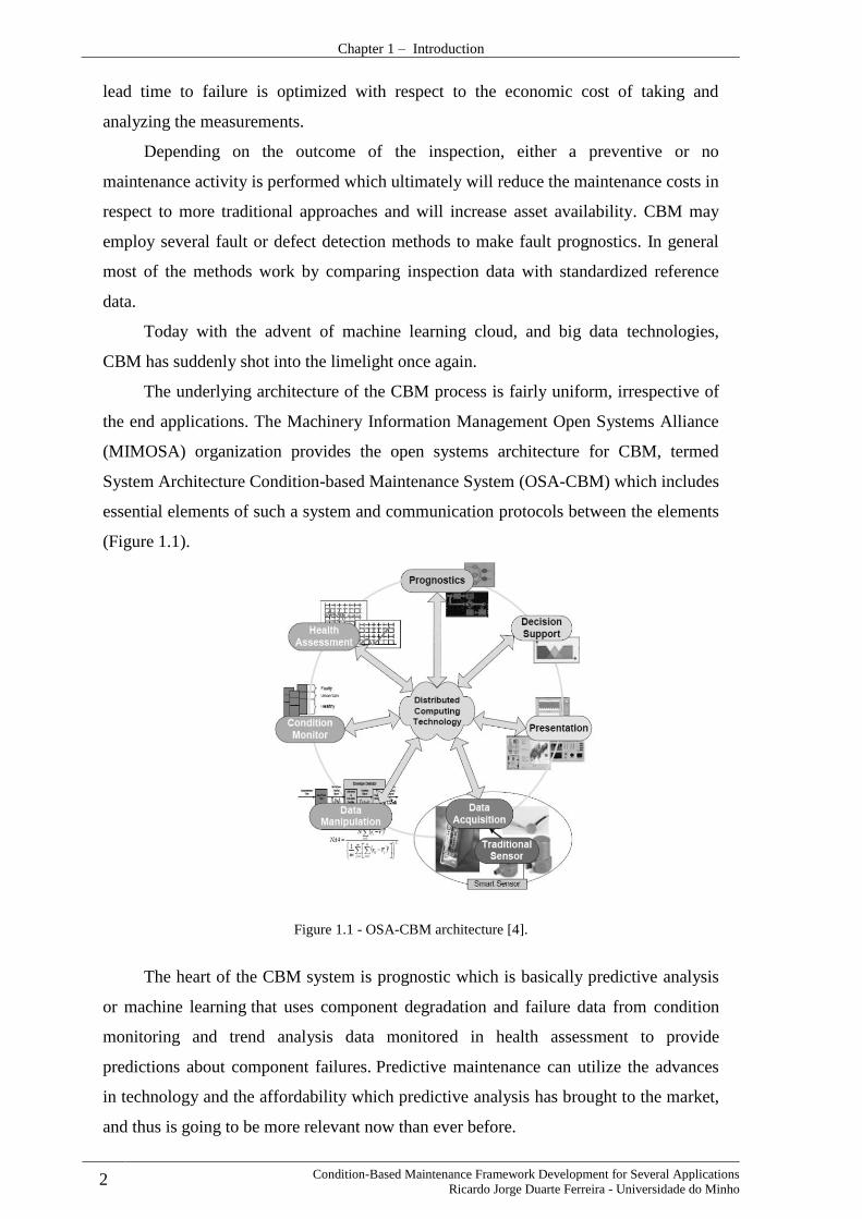
The underlying architecture of the CBM process is fairly uniform, irrespective of
the end applications. The Machinery Information Management Open Systems Alliance
(MIMOSA) organization provides the open systems architecture for CBM, termed
System Architecture Condition-based Maintenance System (OSA-CBM) which includes
essential elements of such a system and communication protocols between the elements
(Figure 1.1).
Figure 1.1 - OSA-CBM architecture [4].
The heart of the CBM system is prognostic which is basically predictive analysis
or machine learning that uses component degradation and failure data from condition
monitoring and trend analysis data monitored in health assessment to provide
predictions about component failures. Predictive maintenance can utilize the advances
in technology and the affordability which predictive analysis has brought to the market,
and thus is going to be more relevant now than ever before.

Chapter 1 – Introduction
Condition-Based Maintenance Framework Development for Several Applications 3 Ricardo Jorge Duarte Ferreira - Universidade do Minho
Organization and Structure of the Thesis 1.3.
In Chapter 1, a small introduction to what is CBM system and what is the problem
that it tries to solve is presented showing also the used approach for implementation and
why it was chosen.
In Chapter 2, a more detailed context to the industry reality regarding
maintenance strategies and where the proposed framework is positioned is presented.
In Chapter 3, is presented all the work developed for Alstom in terms of software
development to support the new monitoring hub for train inspection, which is being
developed on site by them.
In Chapter 4, the work performed for Arrive which is a new project that will
monitor rotational machines of maritime vessels and helicopters, presenting health
indicators regarding asset condition is presented.
In Chapter 5, the developed algorithms for vibration diagnosis and the obtained
values are presented.
4 Condition-Based Maintenance Framework Development for Several Applications
Ricardo Jorge Duarte Ferreira - Universidade do Minho
CHAPTER 2
Maintenance Strategies
Introduction 2.1.
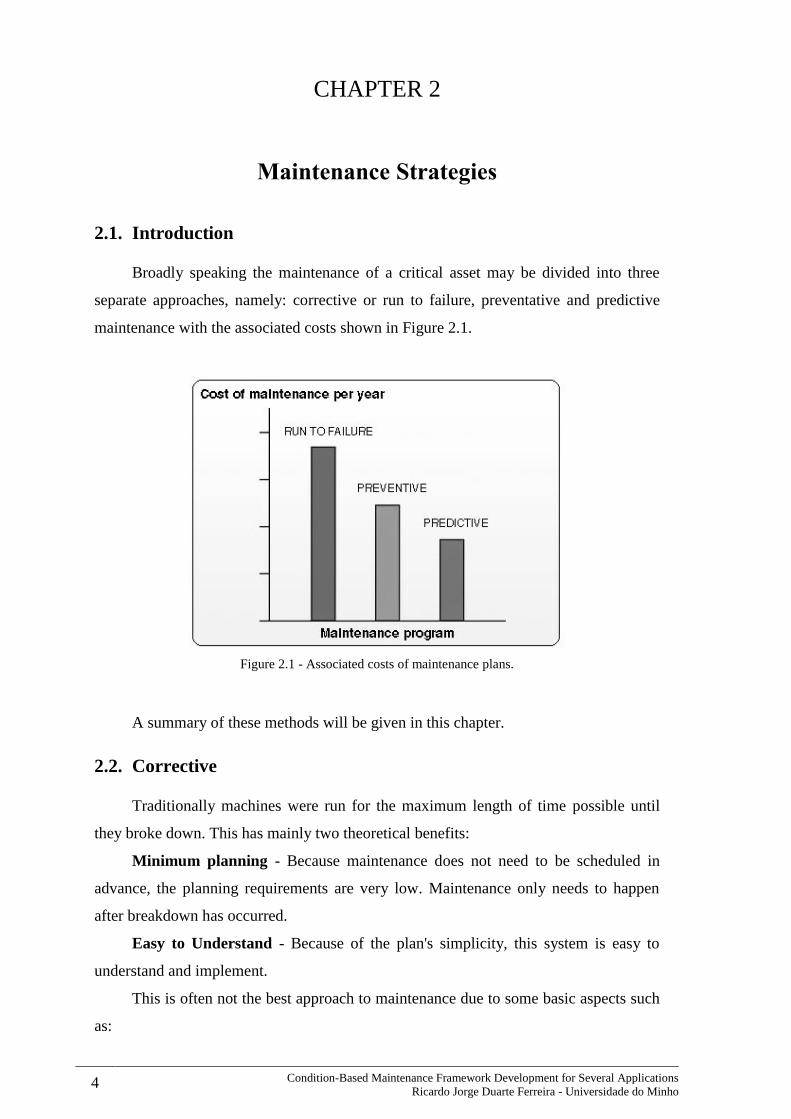
Broadly speaking the maintenance of a critical asset may be divided into three
separate approaches, namely: corrective or run to failure, preventative and predictive
maintenance with the associated costs shown in Figure 2.1.
Figure 2.1 - Associated costs of maintenance plans.
A summary of these methods will be given in this chapter.
Corrective 2.2.
Traditionally machines were run for the maximum length of time possible until
they broke down. This has mainly two theoretical benefits:
Minimum planning - Because maintenance does not need to be scheduled in
advance, the planning requirements are very low. Maintenance only needs to happen
after breakdown has occurred.
Easy to Understand - Because of the plan's simplicity, this system is easy to
understand and implement.
This is often not the best approach to maintenance due to some basic aspects such
as:

Chapter 2 – Maintenance Strategies
Condition-Based Maintenance Framework Development for Several Applications 5 Ricardo Jorge Duarte Ferreira - Universidade do Minho
Unpredictability – Because most asset failures are unpredictable, it is difficult
to anticipate when manpower and parts will be needed for repairs.
Inconsistency – The intermittent nature of failures means the efficient planning
of staff and resources can be difficult.
Costly – All costs associated with this strategy need to be considered when it is
implemented. These costs include production costs and breakdown costs, in
addition to direct parts and labor costs associated with performing the
maintenance.
Inventory Costs – The maintenance team needs to hold spare parts in inventory,
to accommodate for intermittent failures.
Preventive Maintenance 2.3.
The preventive maintenance method uses an estimate for the mean time between
failures of the particular machine to be maintained such that maintenance of key
components may be undertaken at regular intervals shorter than the expected failure
time. It is common to choose the intervals such that no more than 1-2% of the machines
will experience failure within that time. This does mean that the vast majority could
have run longer by a factor of two or three [5].
Preventive Maintenance Plans have the advantage when compared to less
complex strategies. Unplanned, reactive maintenance has many overhead costs that can
be avoided during the planning process. These costs of unplanned maintenance include
lost production, higher costs for parts and shipping, as well as time lost responding to
emergencies and diagnosing faults while equipment is not working. When maintenance
is planned, each of these costs can be reduced. Equipment can be shut down to coincide
with production downtime. Prior to the shutdown, any required parts, supplies and
personnel can be gathered to minimize the time taken for a repair. These measures
decrease the total cost of the maintenance.
Safety is also improved because equipment breaks down less often than for less
complex strategies.
The disadvantage is that the majority of maintenance undertaken via this method
is unnecessary, causing excessive cost of components and machine downtime because
of unpredictable faults. The components to be replaced are often in perfect working
condition and the unnecessary dismantling of a machine causes the risk of faults being

Chapter 2 – Maintenance Strategies
6 Condition-Based Maintenance Framework Development for Several Applications
Ricardo Jorge Duarte Ferreira - Universidade do Minho
introduced where previously none existed. This method does have its place, where the
statistical spread about the mean failure time is small, hence the intervals may be
organized in such a way to minimize cost, though this doesn’t work so well on
components where the failure time less reliably predictable.
Predictive Maintenance 2.4.
Predictive maintenance has two main objectives. Firstly, to predict when
equipment failure might occur, and secondly, to prevent occurrence of the failure by
performing any required maintenance. The task of monitoring for future failure allows
maintenance to be planned before the failure occurs. Ideally, predictive maintenance
allows the maintenance frequency to be as low as possible to prevent unplanned reactive
maintenance, without incurring costs associated with doing too much preventative
maintenance. Predicting failure can be done with one of many techniques. The chosen
technique must be effective at predicting failure and also provide sufficient warning
time for maintenance to be planned and executed.
Condition based maintenance uses measures of specific parameters of a machine
to infer the current condition. This enables identification and diagnosis of faults and
prediction of the remaining useful life (RUL) when compared to baseline results where
the machine is inacceptable working order. This has distinct advantages when compared
to other maintenance schemes, namely:
Increased asset availability: Intelligent maintenance planning is enabled
through the prediction and timely identification of incipient faults within
equipment, thereby reducing the frequency and duration of unplanned
maintenance events. This also supports improved spares management, reduced
revenue losses from unplanned outages and optimal asset management.
Decreased maintenance costs: Fewer maintenance events and fewer
replacements of healthy components.
There are various methods used for obtaining knowledge of the internal condition
of a machine, including vibration analysis, acoustic emission analysis, oil analysis,
thermography, performance analysis, etc...
From all the existing methods, vibration analysis is by far the most used
technique in condition monitoring. The prevalence is due to its quickness (nearly
instantaneous) reaction to changes in machine condition when compared to other
Chapter 2 – Maintenance Strategies
Condition-Based Maintenance Framework Development for Several Applications 7 Ricardo Jorge Duarte Ferreira - Universidade do Minho
methods, such as thermography and oil analysis which will only show significant
changes after the fault is sufficiently developed.
“Vibration has been proven to give the earliest indication of incipient mechanical
defects that are growing slowly over time. If you measure temperature, for example, you
will see a minute change in a bearing’s temperature about two minutes before you have
a catastrophic failure. That’s no good to you.” Steve Boakes, business development
director for General Electric Aviation Systems.
The vast archives of signal processing techniques developed over the past few
decades enable the extraction of minute fault signals which are embedded in noise, or
masked by more prominent signal components.
In an ideal world a CBM system would be able to identify, diagnose and provide
prognosis for all possible faults that may occur with the system being monitored. This is
unfortunately as impractical as it is uneconomical and hence the faults to be identified
must be chosen in such a way to maximize the efficiency of the CBM program e.g.
reduce maintenance costs and unscheduled down time as much as possible to increase
productivity. Also a study needs to be made because sometimes the complexity of the
algorithms and all the investment in data acquisition systems can be so high that isn’t
economically viable.
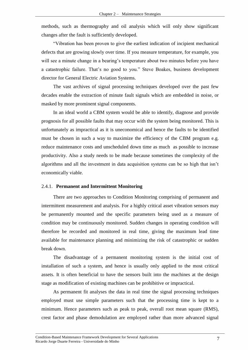
Permanent and Intermittent Monitoring 2.4.1.
There are two approaches to Condition Monitoring comprising of permanent and
intermittent measurement and analysis. For a highly critical asset vibration sensors may
be permanently mounted and the specific parameters being used as a measure of
condition may be continuously monitored. Sudden changes in operating condition will
therefore be recorded and monitored in real time, giving the maximum lead time
available for maintenance planning and minimizing the risk of catastrophic or sudden
break down.
The disadvantage of a permanent monitoring system is the initial cost of
installation of such a system, and hence is usually only applied to the most critical
assets. It is often beneficial to have the sensors built into the machines at the design
stage as modification of existing machines can be prohibitive or impractical.
As permanent fit analyses the data in real time the signal processing techniques
employed must use simple parameters such that the processing time is kept to a
minimum. Hence parameters such as peak to peak, overall root mean square (RMS),
crest factor and phase demodulation are employed rather than more advanced signal

Chapter 2 – Maintenance Strategies
8 Condition-Based Maintenance Framework Development for Several Applications
Ricardo Jorge Duarte Ferreira - Universidade do Minho
processing techniques. These simple parameters give a reduction in lead time before an
impending failure compared to more complex techniques.
The more advanced techniques which may be employed for Condition Monitoring
have a longer processing time than the simple parameters measured above, but give a
far greater picture of the condition of the machine and hence may recognize the onset of
a fault far sooner. Due to the long processing time such techniques are best suited to
intermittent monitoring where the processing of the data is performed at set intervals in
time, say once per month.
Offline CBM systems may be employed to take measurements for intermittent
monitoring, negating the need for expensive permanently fitted transducers. These often
come in the form of a compact console where the transducers are fitted in the desired
location, the data is collected and the unit then performs the relevant processing
techniques and outputs the inferred condition. This has the advantage of allowing time
for the processing of more powerful techniques for greater lead time of diagnosis and
also represents a more versatile method of monitoring as the unit is not fixed and hence
may be employed on a range of machines. An appropriate interval time for
measurement should be employed such that the lead time to failure is optimized with
respect to the economic cost of taking and analyzing the measurements.
Therefore permanent monitoring is used on critical machines to shut them down
in response to an impending failure before catastrophic break down occurs. It is
relatively expensive to set up and gives short lead time before failure due to the
monitoring of simple parameters necessitated by the processing of the data in real time.
Intermittent monitoring employs more advanced signal processing techniques for the
long-term advance warning and diagnosis of incipient faults. It is less expensive to
employ than permanent monitoring, where the main cost occurs in the development of
the analysis algorithms. It is also more versatile and may be used on a wider range of
machines than permanent fit monitoring (due to economic feasibility).
For the most critical assets it is ideal to employ a combination of both permanent
and intermittent monitoring. Unpredictable, sudden break downs may be avoided due to
the application of the permanent fit monitoring, whereas the intermittent monitoring
allows identification of incipient faults giving a greater lead time before break down,
allowing adequate time for maintenance planning and component sourcing.
As stated, the architecture of the CBM process is fairly uniform, irrespective of
the end applications so makes sense in developing a framework based on a known and
acceptable architecture in the field. The focus of the OSA-CBM program is the

Chapter 2 – Maintenance Strategies
Condition-Based Maintenance Framework Development for Several Applications 9 Ricardo Jorge Duarte Ferreira - Universidade do Minho
development of an open standard for distributed CBM software components [6].OSA-
CBM was developed in 2001 by an industry led team partially funded by the Navy
through a Dual Use Science and Technology program. At the time, no framework or
standard existed for implementing CBM systems. The team’s participants covered a
wide range of industrial, commercial, and military applications of CBM technology:
Boeing, Caterpillar, Rockwell Automation, Rockwell Science Center, Newport News
Shipbuilding, and Oceana Sensor Technologies. Other team contributors include the
Penn State University / Applied Research Laboratory and MIMOSA. MIMOSA is a
standard body that manages open information standards for operations and maintenance
in manufacturing, fleet, and facility environments.
OSA-CBM simplifies the integration of a wide variety of software and hardware
components by specifying a standard architecture and framework for implementing
CBM systems. It describes the six functional blocks of CBM systems, as well as the
interfaces between those blocks in conformity with the ISO-13374 (Figure 2.2).
Figure 2.2 - OSA-CBM Functional Block [7].
The benefits from OSA-CBM consist in:
Cost - OSA-CBM can provide significant cost savings because system
integrators and vendors will not have to spend time creating new or proprietary
architectures. Savings will also come from not being committed to single
vendors developing entire CBM systems. Since the standard is broken into
functional components, multiple vendors may compete to develop select blocks
of functionality.

Chapter 2 – Maintenance Strategies
10 Condition-Based Maintenance Framework Development for Several Applications
Ricardo Jorge Duarte Ferreira - Universidade do Minho
Specialization - When vendors are not constrained to providing an entire CBM
system, they can concentrate on one or few areas. The increase in specialization
will allow for better algorithms and technology to be developed. Smaller
companies that could not provide an entire CBM system can now specialize in
one or more of the functional blocks.
Competition - OSA-CBM allows all vendors to use the same input and output
interfaces. The separation of functionality from how the information is presented
to other applications allows direct comparison of the developed functionalities.
Competition now can occur at a functional level, not a system or total solution
level.
Cooperation - Not only can competition increase, but cooperation can also. The
sectioning of CBM into separate independent blocks will allow multiple vendors
to each work on separate modules. Since the standard also defines the interfaces,
each module will be able to communicate with the others seamlessly if
developed using the same technologies.

11 Condition-Based Maintenance Framework Development for Several Applications
Ricardo Jorge Duarte Ferreira - Universidade do Minho
CHAPTER 3
Alstom Health Hub Project
Introduction 3.1.
The Alstom Health Hub (Figure 3.1) is an infrastructure that monitors asset health
and uses advanced data analysis to predict their RUL and replace assets on a truly as-
needed basis. It is supported by monitoring solutions which automatically capture
condition data of rolling stock, infrastructure or signaling assets.
It is an innovative approach designed to shift from traditional mileage-based
maintenance to predictive CBM, thus reducing the lifecycle cost for the operator [8].
Figure 3.1 – Health Hub schematic [8].
The Health Hub is supported by various high technology data capture solutions
allowing the measurement of the condition of three key consumables of a train as it
moves through the portal: wheels, brake pads and pantograph carbon strips.
Figure 3.2 presents a simplified diagram which consists in the overall interaction
between the monitoring systems and the health assessment systems.
Basically each train will have and Radio-Frequency Identification (RFID) which
will firstly be identified in the Health Hub. After the measurement of the condition of
the key consumables of a train, wheels, brake pads and pantograph carbon strips are
acquired.
Chapter 3 – Alstom Health Hub Project
12 Condition-Based Maintenance Framework Development for Several Applications
Ricardo Jorge Duarte Ferreira - Universidade do Minho
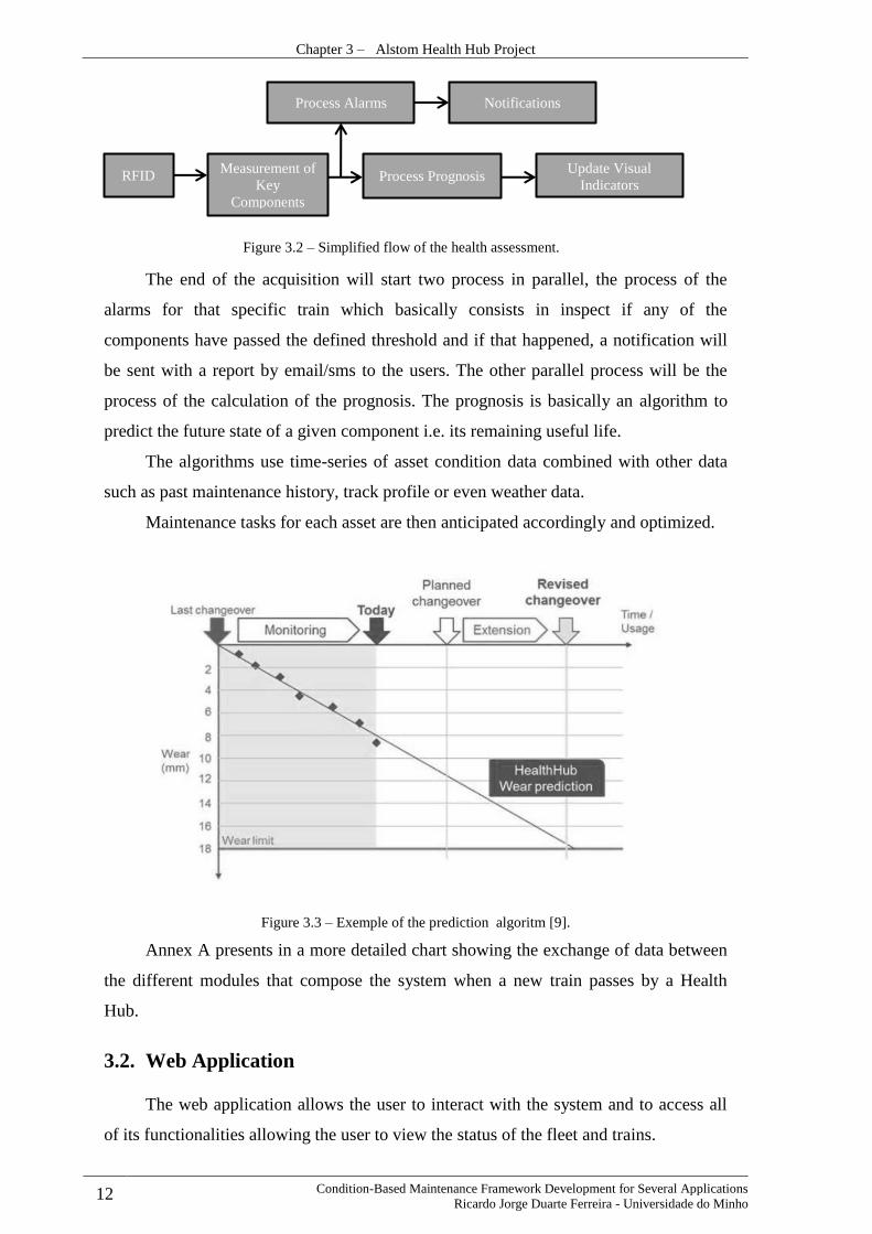
The end of the acquisition will start two process in parallel, the process of the
alarms for that specific train which basically consists in inspect if any of the
components have passed the defined threshold and if that happened, a notification will
be sent with a report by email/sms to the users. The other parallel process will be the
process of the calculation of the prognosis. The prognosis is basically an algorithm to
predict the future state of a given component i.e. its remaining useful life.
The algorithms use time-series of asset condition data combined with other data
such as past maintenance history, track profile or even weather data.
Maintenance tasks for each asset are then anticipated accordingly and optimized.
Figure 3.3 – Exemple of the prediction algoritm [9].
Annex A presents in a more detailed chart showing the exchange of data between
the different modules that compose the system when a new train passes by a Health
Hub.
Web Application 3.2.
The web application allows the user to interact with the system and to access all
of its functionalities allowing the user to view the status of the fleet and trains.
RFID Measurement of
Key
Components
Process Alarms Notifications
Update Visual
Indicators
Figure 3.2 – Simplified flow of the health assessment.
Process Prognosis
Chapter 3 – Alstom Health Hub Project
Condition-Based Maintenance Framework Development for Several Applications 13 Ricardo Jorge Duarte Ferreira - Universidade do Minho
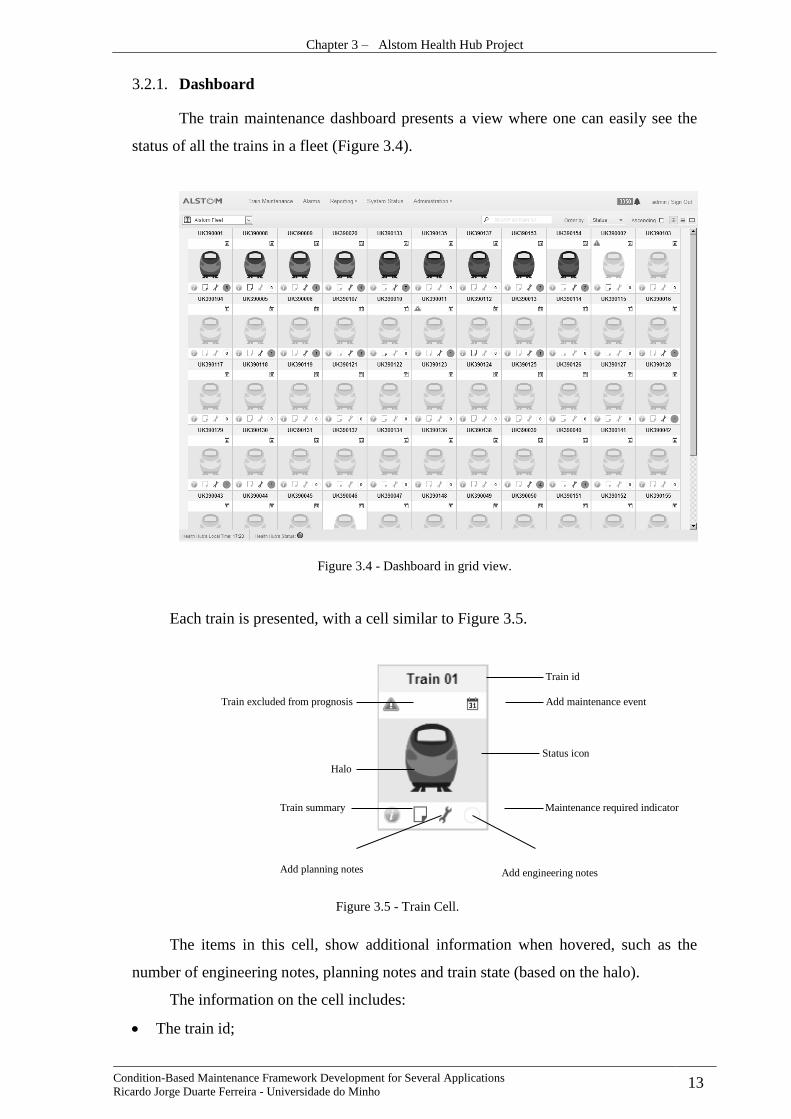
Dashboard 3.2.1.
The train maintenance dashboard presents a view where one can easily see the
status of all the trains in a fleet (Figure 3.4).
Figure 3.4 - Dashboard in grid view.
Each train is presented, with a cell similar to Figure 3.5.
The items in this cell, show additional information when hovered, such as the
number of engineering notes, planning notes and train state (based on the halo).
The information on the cell includes:
The train id;
Add engineering notes Add planning notes
Status icon
Add maintenance event
Maintenance required indicator
Halo
Train id
Train summary
Train excluded from prognosis
Figure 3.5 - Train Cell.

Chapter 3 – Alstom Health Hub Project
14 Condition-Based Maintenance Framework Development for Several Applications
Ricardo Jorge Duarte Ferreira - Universidade do Minho
Its last perceived status: the color of the train icon; it can be one of:
o Grey: no data exists for the train; this should rarely, if ever, happen;
o Green: everything seems to be OK with the train;
o Amber: there may be some problems with the train, but nothing that
requires immediate attention. This can occur when the scrap RUL warning
distance of the train or one of its components is less than the distance to the
train’s next exam.
o Red: some problems with the train require immediate attention. This
can occur when the scrap RUL distance of the train or one of its components
is less than the distance to the train’s next exam.
The train’s halo can indicate a number of issues, dependent on its color. The color it
takes can be one of:
o White: everything is OK.
o Blue: can mean that the train has not been measured since its last
maintenance date, the train has not been measured for at least 3 days, or that
the train has not been measured since the last time an alert was
acknowledged for that train.
o Red: action is required. This can indicate that there are
unacknowledged alerts on the train; that the train is due for service; or that
the train’s expected RUL is less than or equal to zero.
Whether the train has associated with it engineering notes, through a color scheme:
o The train has engineering notes;

Chapter 3 – Alstom Health Hub Project
Condition-Based Maintenance Framework Development for Several Applications 15 Ricardo Jorge Duarte Ferreira - Universidade do Minho
o The train does not have engineering notes.
Whether the train has maintenance notes:
o The train has maintenance notes;
o The train does not have maintenance notes.
Whether the train it has any anomalies:
o The train has associated anomalies;
o The train does not have any associated anomalies;
If a train has been excluded from prognosis, indicated by a warning triangle ( )
Besides presenting this information, by clicking on the summary icon ( ) we are
given a selection of information about the train.
Reports 3.2.2.
The Reports module allows the user to generate the reports available in the SQL
Server Reporting Server (Figure 3.6). These reports are also sent automatically when
any anomaly is detected in the train.
Figure 3.6- Exemple report.
Dynamic and Wear Analysis 3.2.3.
These modules are basically modules that allow the user to display data over time
(Dynamic Analysis) or over the train mileage (Wear Analysis). An example of the Wear
Analysis module is presented in Figure 3.7.

Chapter 3 – Alstom Health Hub Project
16 Condition-Based Maintenance Framework Development for Several Applications
Ricardo Jorge Duarte Ferreira - Universidade do Minho
Figure 3.7 - Wear Analysis display example.
Real-Time Status Information 3.2.4.
The module presents a display similar to that in Figure 3.8. The status of the
Health Hub monitoring systems is indicated by the Red/Green indicators. The example
in Figure 3.8 shows that the Health Hub is currently operating as expected.
Figure 3.8 - The real-time view module.
The indicators in the real-time view are driven by the alerts received from the
subsystems.

Chapter 3 – Alstom Health Hub Project
Condition-Based Maintenance Framework Development for Several Applications 17 Ricardo Jorge Duarte Ferreira - Universidade do Minho
Test Tool 3.2.5.
A request from the client was a tool to test all the features of web application that
could be used by any person without vast software engineering knowledge. Regarding
that a Gui was developed in C# [10] that test every features described in this document
Figure 3.9.
Figure 3.9 – Alstom Health Hub Test Tool.
This tool basically interacts with developed framework in order to simulate the
monitoring systems behavior and test the result in the developed front end. Initially the
tool loads all the trains of the fleet and displays them in a list view.
Figure 3.10 – List with all the fleet trains.
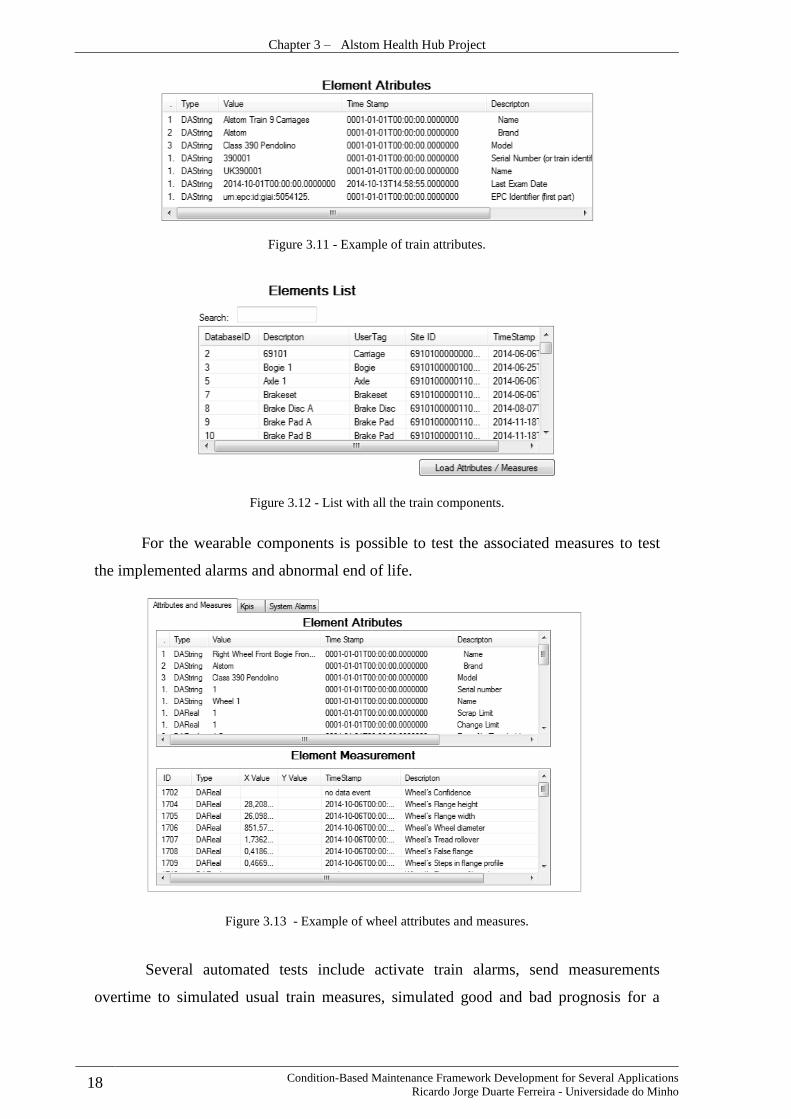
The user is then able to load the train attributes (Figure 3.11) and also load the
train components (Figure 3.12).
Chapter 3 – Alstom Health Hub Project
18 Condition-Based Maintenance Framework Development for Several Applications
Ricardo Jorge Duarte Ferreira - Universidade do Minho
Figure 3.11 - Example of train attributes.
Figure 3.12 - List with all the train components.
For the wearable components is possible to test the associated measures to test
the implemented alarms and abnormal end of life.
Figure 3.13 - Example of wheel attributes and measures.
Several automated tests include activate train alarms, send measurements
overtime to simulated usual train measures, simulated good and bad prognosis for a

Chapter 3 – Alstom Health Hub Project
Condition-Based Maintenance Framework Development for Several Applications 19 Ricardo Jorge Duarte Ferreira - Universidade do Minho
train, automated report generation and user notifications when alarms are generated and
basically almost every developed functionality.
To improve traceability usually each test has a description of the implemented
feature and a link to the client requirement to fundament why that feature was
developed. An example of a test is presented in Figure 3.14
TEST CASE SPECIFICATION
Test Case Identifier: ATHEHUVV-TCS-CSWT-0013
Responsibility: CSWT
Requirement: AHH-124 - ENG-REQ-011
AHH-152 - ENG-REQ-028
Purpose: AHH-321 - Post-processing trigger (Alarms/KPI/Alerts)
Author(s): Ricardo Jorge Duarte Ferreira
Test Item(s):
As the Post-Processing service, I want the common repository to alert me when new measurements are available, so that the various analysis processes can be run on the new data. (This is for the functionality covered within the DE Core).
AC-1: New measurement data triggers an alert to the Post-Processing service AC-2: KPI calculations must be calculated in a specific order NOTE: The trigger mechanism still needs to be agreed by all parties.
Input Specifications: Output Specifications
Step 1 Go to “https://svn/engineering/projects/alstom-transport/ATHEHU-health-hub/work-products/test/GeneralApp” and open the OSACBMSimpleTest application.
Select the desired Train and click "Load Train Elements". Wait for the application load the elements for that train then select the desired element.
In the ‘Several’ tab, click on “Test Cranfield Algorithms”
New measures will be entered into the database for the selected train.
Step 2 Run the following script in the database:
SELECT * FROM DYNAMIC_JOB
WHERE JOB_ID = 1
ORDER BY DJB_CREATION_TIMESTAMP DESC
There will be a recently entered “CranfieldJobExecutor” job in the Dynamic_Job table.
Environment Requirements:
None
Special Procedural Requirements:
To confirm that KPIs are working properly should also be confirmed that the log KPIDemandJob.txt in the scheduler should have no “ERROR” entries.
Inter-case Dependencies:
None
Last execution date:
05-Jul-2014 11:05:19
Current status:
PASSED
Figure 3.14 – Test Example.
In the end, a test matrix was created (Figure 3.15) with the entire tests and the
associated requirements that will then be used in the software acceptance tests.

Chapter 3 – Alstom Health Hub Project
20 Condition-Based Maintenance Framework Development for Several Applications
Ricardo Jorge Duarte Ferreira - Universidade do Minho
Key Summary Test Identifier Status Comments
AHH-105 ENG-REQ-001.1 ATHEHUVV-TCS-CSWT-0001 Passed
AHH-106 ENG-REQ-001.2 ATHEHUVV-TCS-CSWT-0002 Passed
AHH-107 ENG-REQ-001.3 ATHEHUVV-TCS-CSWT-0003 Passed
AHH-108 ENG-REQ-002.1 ATHEHUVV-TCS-CSWT-0004 Passed
AHH-109 ENG-REQ-002.2 ATHEHUVV-TCS-CSWT-0005 Passed
AHH-110 ENG-REQ-002.3 ATHEHUVV-TCS-CSWT-0006 Failed
ATHEHUVV-TCS-CSWT-0007 Passed
AHH-111 ENG-REQ-002.4 ATHEHUVV-TCS-CSWT-0008 Passed
AHH-112 ENG-REQ-003 -- -- Deleted
AHH-113 ENG-REQ-004 -- -- These are not a software requirement, but a reflection of the
expectation has been made clear to
Alstom that this relates mainly to their system availability when in
environment and IT support
service.
AHH-114 ENG-REQ-005.1 -- --
AHH-115 ENG-REQ-005.2 -- --
AHH-116 ENG-REQ-005.3 -- --
Figure 3.15 – Test Matrix.
As the developed software can be reused for different applications with much
less initial effort of implementation so does the test tool, that also can be reused in
different software that uses the same framework with minor changes.

Condition-Based Maintenance Framework Development for Several Applications 21 Ricardo Jorge Duarte Ferreira - Universidade do Minho
CHAPTER 4
Arrive Project
Introduction 4.1.
The Arrive project is a new project that will monitor rotational machines and will
present health indicators regarding asset condition.
The implemented system architecture is based on OSA-CBM similar to Alstom
Health Hub Project. Figure 4.1 represents the interactions of all the intervenient in the
proposed framework.
Figure 4.1 - Interface between the Systems and the Common Repository.
Basically two independent blocks were developed. The data acquisition system
block (Figure 4.1) consists in a GUI (Figure 4.2) that was built in C# language and is
main purpose is to send vibration data to the database. After the data is sent the
diagnostic and prognostic system (Figure 4.1) is triggered. It consists in a web service
that can be deployed on a server and it remains waiting until is triggered with an OSA-
CBM request and is detailed in CHAPTER 5 of this document.

Chapter 4 – Arrive Project
22 Condition-Based Maintenance Framework Development for Several Applications
Ricardo Jorge Duarte Ferreira - Universidade do Minho
This web service consists in calculation of the entire developed algorithms based
on the most recent signal and then the obtained values are sent to the database using
OSA-CBM interface.
Figure 4.2 - Implemented data acquisition system user interface.
Figure 4.3 – Developed system architecture.
Technical Details 4.2.
The technical purpose of vibration CBM is to analyze vibration data in both the
time and frequency domain such that identification, diagnosis and prognosis of incipient
faults may be inferred and the RUL of the asset or component estimated. In its simplest
form this is accomplished by observing changes in specific parameters, such as the
overall RMS value; when the value increases above a certain threshold relative to a
Chapter 4 – Arrive Project
Condition-Based Maintenance Framework Development for Several Applications 23 Ricardo Jorge Duarte Ferreira - Universidade do Minho
baseline value the existence of a fault is implied. Various signal processing techniques
may be employed to reduce background noise and separate out key features in the signal
such that specific faults may be identified and diagnosed.
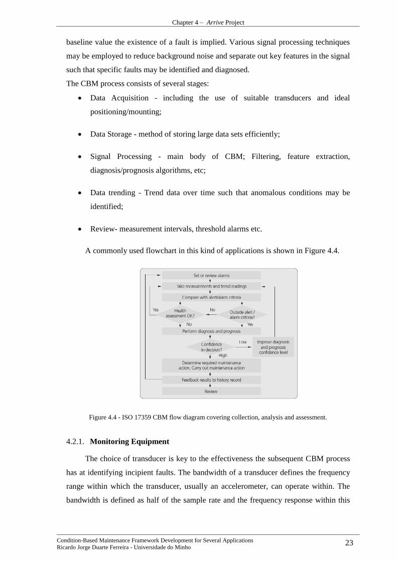
The CBM process consists of several stages:
Data Acquisition - including the use of suitable transducers and ideal
positioning/mounting;
Data Storage - method of storing large data sets efficiently;
Signal Processing - main body of CBM; Filtering, feature extraction,
diagnosis/prognosis algorithms, etc;
Data trending - Trend data over time such that anomalous conditions may be
identified;
Review- measurement intervals, threshold alarms etc.
A commonly used flowchart in this kind of applications is shown in Figure 4.4.
Figure 4.4 - ISO 17359 CBM flow diagram covering collection, analysis and assessment.
Monitoring Equipment 4.2.1.
The choice of transducer is key to the effectiveness the subsequent CBM process
has at identifying incipient faults. The bandwidth of a transducer defines the frequency
range within which the transducer, usually an accelerometer, can operate within. The
bandwidth is defined as half of the sample rate and the frequency response within this

Chapter 4 – Arrive Project
24 Condition-Based Maintenance Framework Development for Several Applications
Ricardo Jorge Duarte Ferreira - Universidade do Minho
range is usually defined as flat within +/-3dB, therefore a sample rate must be chosen
that is at least twice as large as the maximum frequency intended to be measured.
Attention must also be paid to the resonance frequency of the accelerometer as
this will cause a marked deviation from the +/-3dB flat response. Most accelerometers
are designed such that the resonant frequency is well above the maximum frequency to
be measured, though insufficient mounting methods may cause this resonance to lower
into the measurement range.
In the current project, two approaches were followed for the data acquisition. The
first approach was done using a presented in Figure 4.5 which is a Phidgets Spatial.
Figure 4.5 - Phidgets Spatial [11].
This is a relatively inexpensive accelerometer with a short bandwidth of 497Hz
and a maximum acceleration measurement of +/-2g. A good advantage of this system is
that it provides support for several programming languages with a simple search in the
Internet. Due to the short bandwidth and small measurement range limitations are made
on the type of fault which this accelerometer will be able to detect under given
circumstances. Figure 4.6 is a typical trouble shooting table for vibration condition
monitoring. As can be seen many faults occur within the first or second harmonics of
the shaft rotational speed hence the bandwidth of the Phidgets accelerometer is adequate
for those particular faults up to rotational speeds of approximately 15000 rpm such that
the second harmonic is captured. The assets of interest in this project, namely marine
craft rarely exceed rotational speeds of 2000RPM hence the Phidgets accelerometer has
a broad band width enough to capture the first 14 harmonics (at 2000RPM).
Trouble arises when attempting to extract features specific to gear or bearing
faults as they occur at frequencies many times above the rotational speed of the shaft.
For instance the gear meshing frequency about which side bands occur which are
indicative of the state of the gears occurs at a frequency equal to the number of gear
teeth multiplied by the RPM of the gear wheel. Hence depending on the number of teeth
on the gear wheel the meshing frequency could occur well outside the range of 500Hz,

Chapter 4 – Arrive Project
Condition-Based Maintenance Framework Development for Several Applications 25 Ricardo Jorge Duarte Ferreira - Universidade do Minho
making the identification of gear faults impossible. For more detail on usual vibration
faulty components see Figure 4.6.
Figure 4.6 - Typical vibration trouble shooting chart for CBM .
Another approach for acquiring vibration was also tested using a high spec data
acquisition system from Beran (Figure 4.7) that allows more focus on the signal
processing techniques.
Figure 4.7 - Beran 720 Auxiliary Plant Monitor [12].
This is a much more advance acquisition system and its main features are:
Specifications:
Dimensions (mm) 3 60 x 140 x 60
Measurement Inputs 16 channels of vibration or process inputs: accelerometer; velocity
transducer; eddy current
probe; process inputs, e.g. 4-20mA, 0-1V, 0-10V
Acquisition Vibration/process: 24-bit A/D converters with 20kHz bandwidth per
channel
Speed Inputs 4 channels including power output for transducers
Chapter 4 – Arrive Project
26 Condition-Based Maintenance Framework Development for Several Applications
Ricardo Jorge Duarte Ferreira - Universidade do Minho
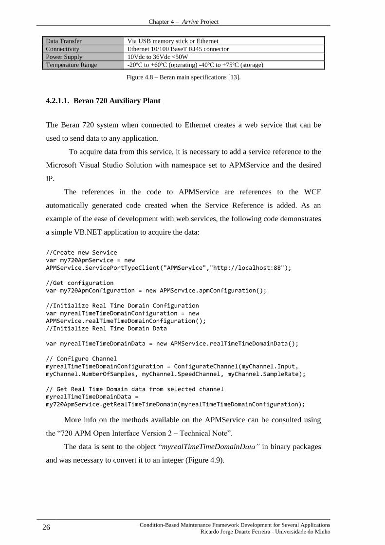
Data Transfer Via USB memory stick or Ethernet
Connectivity Ethernet 10/100 BaseT RJ45 connector
Power Supply 10Vdc to 36Vdc <50W
Temperature Range -20ºC to +60ºC (operating) -40ºC to +75ºC (storage)
Figure 4.8 – Beran main specifications [13].
4.2.1.1. Beran 720 Auxiliary Plant
The Beran 720 system when connected to Ethernet creates a web service that can be
used to send data to any application.
To acquire data from this service, it is necessary to add a service reference to the
Microsoft Visual Studio Solution with namespace set to APMService and the desired
IP.
The references in the code to APMService are references to the WCF
automatically generated code created when the Service Reference is added. As an
example of the ease of development with web services, the following code demonstrates
a simple VB.NET application to acquire the data:
//Create new Service var my720ApmService = new APMService.ServicePortTypeClient("APMService","http://localhost:88"); //Get configuration var my720ApmConfiguration = new APMService.apmConfiguration(); //Initialize Real Time Domain Configuration var myrealTimeTimeDomainConfiguration = new APMService.realTimeTimeDomainConfiguration(); //Initialize Real Time Domain Data var myrealTimeTimeDomainData = new APMService.realTimeTimeDomainData(); // Configure Channel myrealTimeTimeDomainConfiguration = ConfigurateChannel(myChannel.Input, myChannel.NumberOfSamples, myChannel.SpeedChannel, myChannel.SampleRate); // Get Real Time Domain data from selected channel myrealTimeTimeDomainData = my720ApmService.getRealTimeTimeDomain(myrealTimeTimeDomainConfiguration);
More info on the methods available on the APMService can be consulted using
the “720 APM Open Interface Version 2 – Technical Note”.
The data is sent to the object “myrealTimeTimeDomainData” in binary packages
and was necessary to convert it to an integer (Figure 4.9).

Chapter 4 – Arrive Project
Condition-Based Maintenance Framework Development for Several Applications 27 Ricardo Jorge Duarte Ferreira - Universidade do Minho
Figure 4.9 – Data Received from the APM Service.
Has the data is coming in pack of 3, first was necessary to combine all the packs
in binary string. This was done using the following lines of code:
// Shift the data to 24 bits int[] CurrentBinary = new int[3]; CurrentBinary[i] = 0; CurrentBinary[i] = myrealTimeTimeDomainData.data.Value[refField] << 8; CurrentBinary[i] = CurrentBinary[i] + myrealTimeTimeDomainData.data.Value[refField + 1] << 8;
CurrentBinary[i]=CurrentBinary[i]+
myrealTimeTimeDomainData.data.Value[refField + 2];
After having the full value in a string, was necessary to convert it to a 32 bit
binary string in order to use the method “Convert.ToInt32”. This was done using the
following lines:
//Convert 24 bits to 32 bits signed and convert to scaling units CurrentBinaryString[i] = Convert.ToString(CurrentBinary[i], 2).PadLeft(24, '0'); CurrentBinaryString[i] = CurrentBinaryString[i].PadLeft(32, CurrentBinaryString[i][0]);
Current[i]=Convert.ToInt32(CurrentBinaryString[i],2)
*myrealTimeTimeDomainData.sampleScalingFactor;
The corresponding Speed Channel is easily supplied using the simple method:
//Acquire Speed Value RPMSpeed = myrealTimeTimeDomainData.speedRpm;
To send then the values to the Database, is necessary to build
“OSACBMHealthHubDataService.Site”. An Example is shown below:

Chapter 4 – Arrive Project
28 Condition-Based Maintenance Framework Development for Several Applications
Ricardo Jorge Duarte Ferreira - Universidade do Minho
var elementSite = new OSACBMHealthHubDataService.Site() {
//example of site constrution from DAPort (section 5.1.2.1) category = OSACBMHealthHubDataService.SITE_CATEGORY.SITE_SPECIFIC, siteId = DatabaseId, userTag = "APMChannel”, regId = MIMOSA_REGID, systemUserTag = HEALTH_HUB_NAME
};
After build the site, is necessary to set send the data. As it’s intended to send two
different measures, the “OSACBMHealthHubDataService.DataEvent” is initialized like
the following:
//now set the measure data values var dataToSet = new OSACBMHealthHubDataService.DataEvent[2]; It is also necessary to define a timestamp for the data. This can be done using the “OSACBMHealthHubDataService.OsacbmTime()”: var measureTimestamp = new OSACBMHealthHubDataService.OsacbmTime() { time_type = OSACBMHealthHubDataService.OsacbmTimeType.OSACBM_TIME_MIMOSA, time = DateTime.UtcNow.ToString("O") };
After it is possible to send the values for Speed and Current measures:
//Send Speed Measure to Database SetDataEvent(ref dataToSet, ref pos, elementSite, measureTimestamp, ANM_ID_Speed, currentvalue.SpeedValue); // Send current Values to Database SetDataEvent(ref dataToSet, ref pos, elementSite, measureTimestamp, ANM_ID_Current, currentvalue.CurrentValue, currentvalue.Time); var measureDataSet = new OSACBMHealthHubDataService.DataEventSet() { site = elementSite, id = Convert.ToUInt32(elementId), time = measureTimestamp, dataEvents = dataToSet }; var setDataResultStatus = serviceDataProxy.serviceNotifyDataEventSet(measureDataSet); System.Console.WriteLine("Set measure data return: [\n{0}\n]", setDataResultStatus);
If the data was sent to the database successfully a message is displayed saying the
transaction was “OK”.
After sending all the values is necessary to inform the “Front End Interface” that
new data is available in order to trigger the processing of the algorithms.
This is done using the following lines:

Chapter 4 – Arrive Project
Condition-Based Maintenance Framework Development for Several Applications 29 Ricardo Jorge Duarte Ferreira - Universidade do Minho
//finish indication serviceProxy.epNotifyApp( new OSACBMConfigurationLibraryService.Parameter[4] { new OSACBMConfigurationLibraryService.GeneralParameter(){datatype=OSACBMConfigurationLibraryService.XmlDataType.@string, name="MEASURESETFINISH", value="ROOF"}, new OSACBMConfigurationLibraryService.GeneralParameter(){datatype=OSACBMConfigurationLibraryService.XmlDataType.@string, name="RFID", value=CurrentValues[0].Channel.ParentSiteId}, new OSACBMConfigurationLibraryService.GeneralParameter(){datatype=OSACBMConfigurationLibraryService.XmlDataType.@string, name="HEALTHHUB", value=HEALTH_HUB_NAME}, new OSACBMConfigurationLibraryService.GeneralParameter(){datatype=OSACBMConfigurationLibraryService.XmlDataType.dateTime,name="TIMESTAMP", value=measureTimestamp.time}, } );
This will insert in the table Dynamic_Jobs, a job indicating that new data was
received for the selected Data Acquisition System like showed in Figure 4.10.
Figure 4.10 - Dynamic Job Exemple.
It is possible to see the last two jobs were already processed by the Algorithms,
and the date that they were calculated is showed in
“DJB_LAST_UPDATE_TIMESTAMP”. The first job has the DJB_STATE = 0 and
was not processed yet. As soon as the Scheduling System is installed on the System and
his Started, we will try to connected to the Front End Application that there is a new job
every time a DJB_STATE = 0.
Fault Characteristics 4.2.2.
Within a complex machine such as a marine vessel engine, there are many sources
of malfunction.
Faults may be identified by changes in the vibratory characteristics specific to the
operation of the component in question under normal operation. For instance a shaft
imbalance will cause an increase in out-of-balance forces and therefore cause an
increase in the first harmonic of the shafts rotational speed. Some common faults can
be:
Shaft imbalance - manifests in the first harmonic of the shafts rotational speed.
Out of balance forces are defined as follows:

Chapter 4 – Arrive Project
30 Condition-Based Maintenance Framework Development for Several Applications
Ricardo Jorge Duarte Ferreira - Universidade do Minho
𝐹 = 𝑚𝑒𝜔2
Where m is the unbalanced mass, e is the radius of eccentricity and 𝜔 is the
angular velocity. Hence the out of balance force will increase proportional to the
angular velocity squared, this may be utilized when order tracking.
Misalignment - Commonly cited as a large twice running speed (2x) and/or
running speed (1x) vibration component, though there is much debate as to the
physical reason (Al-Hussain).
Mechanical Looseness - Second harmonic of shaft speed.
Gear faults - chipped/ cracked tooth, missing tooth, manifests as asymmetries in
the side bands about the gear meshing frequency. The gear meshing frequency
may be defined as follows:
𝑓𝐺𝑀 = 𝑁 x 𝑓𝑟
Where 𝑓𝐺𝑀 is the gear meshing frequency (Hz), N is the number of gear teeth and
𝑓𝑟 is the rotation speed of the gear (Hz). Side bands will then be spaced about the gear
meshing frequency at frequency intervals equal to the shaft rotational speed.
Bearing faults - many times the rotational speed of the shaft. Four generalized
faults may be identified; ball damage, inner race defect, outer race defect and
cage damage. Figure 4.11 shows a diagram of a typical rolling element bearing
with relevant dimensions and frequencies [14].
Figure 4.11 - Dimensions and fault frequencies of typical rolling element bearing [13].
The fault frequencies of interest are as follows:

Chapter 4 – Arrive Project
Condition-Based Maintenance Framework Development for Several Applications 31 Ricardo Jorge Duarte Ferreira - Universidade do Minho
𝐹𝐶𝐹 =1
2𝐹𝑅(1 −
𝐷𝐵
𝐷𝑃cos 𝜃)
𝐹𝑂𝑅𝐹 =𝑁𝐵
2𝐹𝑅(1 −
𝐷𝐵
𝐷𝑃cos 𝜃)
𝐹𝐼𝑅𝐹 =𝑁𝐵
2𝐹𝑅(1 +
𝐷𝐵
𝐷𝑃cos 𝜃)
𝐹𝐵𝐹 =𝐷𝑝
2𝐷𝐵𝐹𝑅(1 − [
𝐷𝐵
𝐷𝑃cos 𝜃]2)
Where 𝐹𝑅 is the shaft rotational speed (Hz), 𝐹𝐶𝐹is the cage fault frequency (Hz),
𝐹𝑂𝑅𝐹is the outer race fault frequency (Hz), 𝐹𝐼𝑅𝐹is the inner race fault frequency (HZ),
𝐹𝐵𝐹 is the ball fault frequency (Hz), 𝐷𝐵 is the ball diameter (m), 𝐷𝑃 is the pitch diameter
(m), 𝑁𝐵 is the number of rolling elements and 𝜃 is the ball contact angle.
For more information on bearings see reference to [15]. For information on gear
faults see references [16], [17], [18], [19], [20], [21].
Signal processing 4.3.
The raw data gathered from the transducer, once stored adequately, yields very
little information in terms of identification of key parameters indicative of the machines
condition. Signal processing techniques must be employed to de-noise the raw data and
extract key features specific to faults of interest.
Vibration signals are initially obtained as a series of digital values representing
proximity, velocity, or acceleration in the time domain. This section reviews recent
research on vibration techniques in the time domain for various types of rotating
machinery and categorizes these techniques into the following groups.
Time Domain 4.3.1.
Vibration signals are initially obtained as a series of digital values representing
proximity, velocity, or acceleration in the time domain. This section reviews recent
research on vibration techniques in the time domain for various types of rotating
machinery and categorizes these techniques into the following groups (Figure 4.12).
4.3.1.1. Statistical parameters
Various parameters exist which may be used as indicators of a machines
condition. The following whole vibration parameters are relatively simple to compute
requiring little computing power. These have the benefit that they may be computed in
real time and hence lend themselves well to on-line permanent fit CBM. The RMS
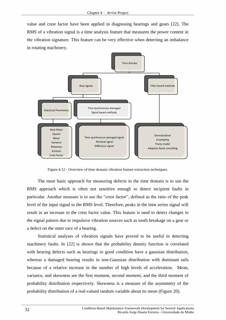
Chapter 4 – Arrive Project
32 Condition-Based Maintenance Framework Development for Several Applications
Ricardo Jorge Duarte Ferreira - Universidade do Minho
value and crest factor have been applied in diagnosing bearings and gears [22]. The
RMS of a vibration signal is a time analysis feature that measures the power content in
the vibration signature. This feature can be very effective when detecting an imbalance
in rotating machinery.
Figure 4.12 - Overview of time domain vibration feature extraction techniques.
The most basic approach for measuring defects in the time domain is to use the
RMS approach which is often not sensitive enough to detect incipient faults in
particular. Another measure is to use the “crest factor”, defined as the ratio of the peak
level of the input signal to the RMS level. Therefore, peaks in the time series signal will
result in an increase in the crest factor value. This feature is used to detect changes in
the signal pattern due to impulsive vibration sources such as tooth breakage on a gear or
a defect on the outer race of a bearing.
Statistical analyses of vibration signals have proved to be useful in detecting
machinery faults. In [22] is shown that the probability density function is correlated
with bearing defects such as bearings in good condition have a gaussian distribution,
whereas a damaged bearing results in non-Gaussian distribution with dominant tails
because of a relative increase in the number of high levels of acceleration. Mean,
variance, and skewness are the first moment, second moment, and the third moment of
probability distribution respectively. Skewness is a measure of the asymmetry of the
probability distribution of a real-valued random variable about its mean (Figure 20).
Time domain
Raw signals
Statistical Parameters
Root Mean Square Mean
Variance Skewness Kurtosis
Crest Factor
Time Synchronous Averaged Signal based methods
Time synchronous averaged signal Residual signal
Difference signal
Filter based methods
Demodulation Enveloping
Prony model
Adaptive Noise cancelling

Chapter 4 – Arrive Project
Condition-Based Maintenance Framework Development for Several Applications 33 Ricardo Jorge Duarte Ferreira - Universidade do Minho
Figure 4.13 - Demonstration of Skewness Coefficient [23].
Kurtosis is defined as the fourth moment of the distribution and measures the
relative flatness of a distribution as compared to a normal distribution. Kurtosis
provides a measure of the size of the tails of distribution and is used as an indicator of
major peaks in a set of data.
It is defined as the normalized fourth central moment of a distribution:
Using this definition the value of kurtosis for a normal distribution is 3. A second
definition maybe be that the value of kurtosis for the normal distribution is 0. This is
defined as the fourth cumulant of the distribution divided by the second cumulant:
As the kurtosis of a distribution is a measure of the distributions peakness it may
be used to identify impulsive components within a time signal. This applies particularly
well to bearing faults where a defect will cause periodic impulsive impacts once per
revolution. Hence kurtosis values of time series may be trended over time, where a
significant increase will indicate the presence of a fault.
This technique can often become unstuck when the signals are highly embedded
in noise as the kurtosis no longer captures the impulsive signature, causing a faulty
signal to have similar kurtosis values as a healthy signal. This problem can be
formulated as “detecting transient signals in strong additive noise”. Here kurtosis will
generate high values in the presence of a fault provided the impacts are sufficiently well
separated and the signal-to-noise ratio is sufficiently high [24]. As may be seen in
Figure 4.14 showing a typical vibration signature of a rolling element bearing fault the
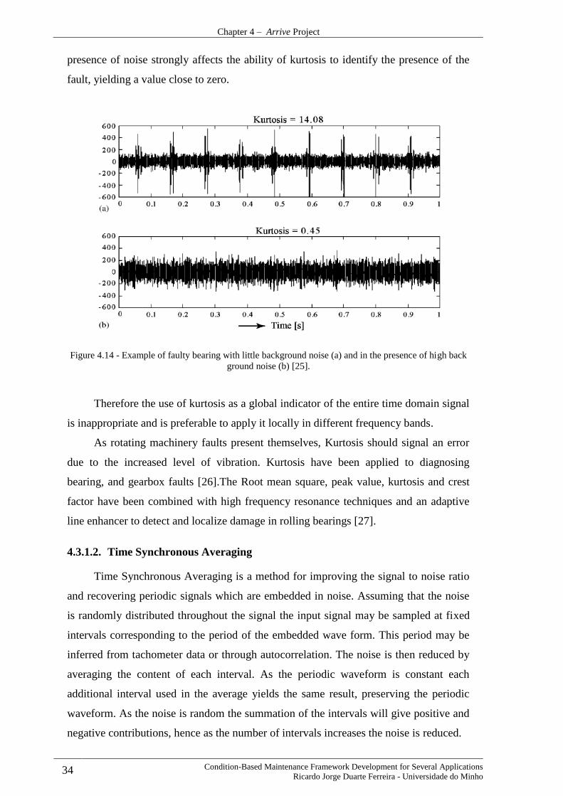
Chapter 4 – Arrive Project
34 Condition-Based Maintenance Framework Development for Several Applications
Ricardo Jorge Duarte Ferreira - Universidade do Minho
presence of noise strongly affects the ability of kurtosis to identify the presence of the
fault, yielding a value close to zero.
Figure 4.14 - Example of faulty bearing with little background noise (a) and in the presence of high back
ground noise (b) [25].
Therefore the use of kurtosis as a global indicator of the entire time domain signal
is inappropriate and is preferable to apply it locally in different frequency bands.
As rotating machinery faults present themselves, Kurtosis should signal an error
due to the increased level of vibration. Kurtosis have been applied to diagnosing
bearing, and gearbox faults [26].The Root mean square, peak value, kurtosis and crest
factor have been combined with high frequency resonance techniques and an adaptive
line enhancer to detect and localize damage in rolling bearings [27].
4.3.1.2. Time Synchronous Averaging
Time Synchronous Averaging is a method for improving the signal to noise ratio
and recovering periodic signals which are embedded in noise. Assuming that the noise
is randomly distributed throughout the signal the input signal may be sampled at fixed
intervals corresponding to the period of the embedded wave form. This period may be
inferred from tachometer data or through autocorrelation. The noise is then reduced by
averaging the content of each interval. As the periodic waveform is constant each
additional interval used in the average yields the same result, preserving the periodic
waveform. As the noise is random the summation of the intervals will give positive and
negative contributions, hence as the number of intervals increases the noise is reduced.

Chapter 4 – Arrive Project
Condition-Based Maintenance Framework Development for Several Applications 35 Ricardo Jorge Duarte Ferreira - Universidade do Minho
Let the input 𝑓(𝑡) be composed of a repetitive signal 𝑠(𝑡) and noise 𝑛(𝑡). Say the
kth repetition of 𝑠(𝑡)begins at time 𝑡𝑘 (where t1=0) and that the sample are taken every T
seconds. Then;
𝑓(𝑡) = 𝑠(𝑡) + 𝑛(𝑡)
This signal is then sampled, with sample values
𝑓(𝑡𝑘 + 𝑖𝑇) = 𝑠(𝑡𝑘 + 𝑖𝑇) + 𝑛(𝑡𝑘 + 𝑖𝑇)
= 𝑠(𝑖𝑇) + 𝑛(𝑡𝑘 + 𝑖𝑇)
It may be assumed that in a usual situation the average of the noise contributions
is zero, with a constant RMS value 𝜎. For the ith sample point the signal to noise ratio,
S/N, may therefore be calculated as:
𝑆
𝑁=
𝑠(𝑖𝑇)
𝜎
After m repetitions the value stored in the ith memory location is given by:
∑ 𝑓(𝑡𝑘 + 𝑖𝑇) = ∑ 𝑠(𝑖𝑇) + ∑ 𝑛(𝑡𝑘 + 𝑖𝑇)
𝑚
𝑘=1
𝑚
𝑘=1
𝑚
𝑘=1
= 𝑚𝑠(𝑖𝑇) + ∑ 𝑛(𝑡𝑘 + 𝑖𝑇)
𝑚
𝑘=1
Since the noise is random and the m samples are independent the mean RMS of
the sum of the m noise samples is m𝜎2, hence the RMS value is √𝑚𝜎. Therefore the
new signal to noise ratio is:
(𝑆
𝑁)𝑚 = √𝑚(
𝑆
𝑁)
The signal to noise ratio is improved by a factor of m1/2
[28].
In practice this principle is simple, usually consisting in placing the vibration
sensor on the machine to be diagnosed and use a remote optical sensor or stroboscope
with a trigger output to accurately determine the exact speed of the machine (Figure
4.15).
This external trigger will initialize the vibration data collector and with the use of
a high number of averages can eliminate “cross-talk” signals and improve signal-to-
noise ratio.
A simple example of the all process can be seen in Figure 4.16.
If this external trigger is unavailable a sync period may be found using several
techniques (Autocorrelation, Fourier Transform, etc). Using these techniques a suitable
period can be identified and can be used in the signal averaging technique.

Chapter 4 – Arrive Project
36 Condition-Based Maintenance Framework Development for Several Applications
Ricardo Jorge Duarte Ferreira - Universidade do Minho
Figure 4.15 - Common Set-up for synchronous time averaging.
Figure 4.16 – Schematic of “Time Synchronous Averaging” algorithm [29].
4.3.1.3. Filter based methods
Demodulation including phase and amplitude demodulation is an important signal
processing technique. The amplitude demodulation, also known as envelop, or
resonance demodulation, or high frequency resonance demodulation techniques
separates low-level, low-frequency signals from background noise, enabling them to be
easily measured. In the application of gear faults detection, the amplitude demodulation

Chapter 4 – Arrive Project
Condition-Based Maintenance Framework Development for Several Applications 37 Ricardo Jorge Duarte Ferreira - Universidade do Minho
focused on the fault-induced high-order modulation sidebands around the dominant gear
meshing harmonic.
Many faults such as bearing and gearbox faults cause a modulation in the
amplitude of the vibration signal. This is caused by impulsive strikes such as a missing
tooth on a gear set or cracks in the inner race of a bearing cage. This impulsive strike
will excite the natural resonance of the structure, but as the strike is of a very short
duration the energy will be spread across many harmonics and hence will have low
amplitude and the fault signal is always masked by noise and low frequency effects
[30].
Envelope analysis enables the transient fault signals to be separated from any
masking features such as background noise and frequency components due to other
oscillatory forces (shaft rotation etc.).
A relatively simple processing method for envelope analysis may be seen in
Figure 4.17 and may be described as follows. Firstly a high pass or band pass filter is
applied to the raw time data as the transient faults are generally of high frequency
corresponding, in the case of rolling element bearings. The filtered signal will be a
modulated time waveform which is then rectified such that all negative amplitudes are
made positive. The signal is then low pass filtered to output the enveloped signal which
may then be frequency analyzed, the spectral content of which will signify the severity
of the fault. For instance, a highly modulated signal once processed will produce large
spectral content corresponding to the fault frequency and harmonics. A healthy signal
will be minimally modulated producing little frequency content.
Figure 4.18 shows the enveloped vibration spectrum of a bearing in faulty and
healthy condition. As can be seen there is far more frequency content attributed to the
faulty bearing than there is to the healthy bearing. This may be used to indicate the
bearings health and thresholds on the spectrum may be set at specific fault frequencies
such that alarms may sound when the fault is sufficiently developed.

Chapter 4 – Arrive Project
38 Condition-Based Maintenance Framework Development for Several Applications
Ricardo Jorge Duarte Ferreira - Universidade do Minho
Figure 4.17 - Demodulation process [28].
Figure 4.18 - Comparison of enveloped vibration spectra for faulty and healthy bearings [31].
There are several methods for the estimation of the signals envelope, the above
being a more basic approach. Another method employs is the Empirical Mode
Decomposition (EMD) algorithm. The implementation of this technique can be resumed
in the following steps:
Identify local maxima and minima in the signal;
Deduce an upper and a lower envelope by interpolation (cubic splines);

Chapter 4 – Arrive Project
Condition-Based Maintenance Framework Development for Several Applications 39 Ricardo Jorge Duarte Ferreira - Universidade do Minho
o subtract the mean envelope from the signal
o iterate until extremes = zeroes +1
Subtract the so-obtained Intrinsic Mode Function (IMF) from the signal;
Iterate on the residual.
Figure 4.19 demonstrates an example of the iteration steps on the EMD algorithm
which is called “Shifting”. In the end of the process a signal decomposition is achieved
and is expected that the number of extreme will decrease as the procedure continues, so
that the signal is sequent decomposed into the highest frequency component “imf1” to
the lowest frequency component “imfn”, for some finite n and a residue signal r [32].
Finally, for the signal shown above the decomposition signals are shown in Figure
4.20.
Figure 4.19 - Empirical Mode Decomposition Iteration [33].

Chapter 4 – Arrive Project
40 Condition-Based Maintenance Framework Development for Several Applications
Ricardo Jorge Duarte Ferreira - Universidade do Minho
Figure 4.20 - Empirical Mode Decomposition Signals [33].
Frequency Domain and Time Frequency Domain Feature Extraction 4.3.2.
Techniques
Features regarding frequency information such as frequency domain features and
time frequency domain features are being widely investigated at present. These features
can generally indicate machinery faults better than time domain vibration features
because characteristic frequency components such as resonance frequency components
or defect frequency components can be relatively easily detected and matched to faults.
4.3.2.1. Fast Fourier Transform
The Fast Fourier Transform (FFT) is the most conventional diagnosis technique
and has been widely used to identify the frequency features of signals. These signals can
be raw signals or processed signals.
There are vast amounts of literature covering the technical details of the Fourier
transform and FFT, so technical details will be omitted here.
Mathematically, the process of Fourier analysis is represented by the Fourier
transform:
This means that FFT is the sum over all time of the signal 𝑓(𝑡) multiplied by a
complex exponential.
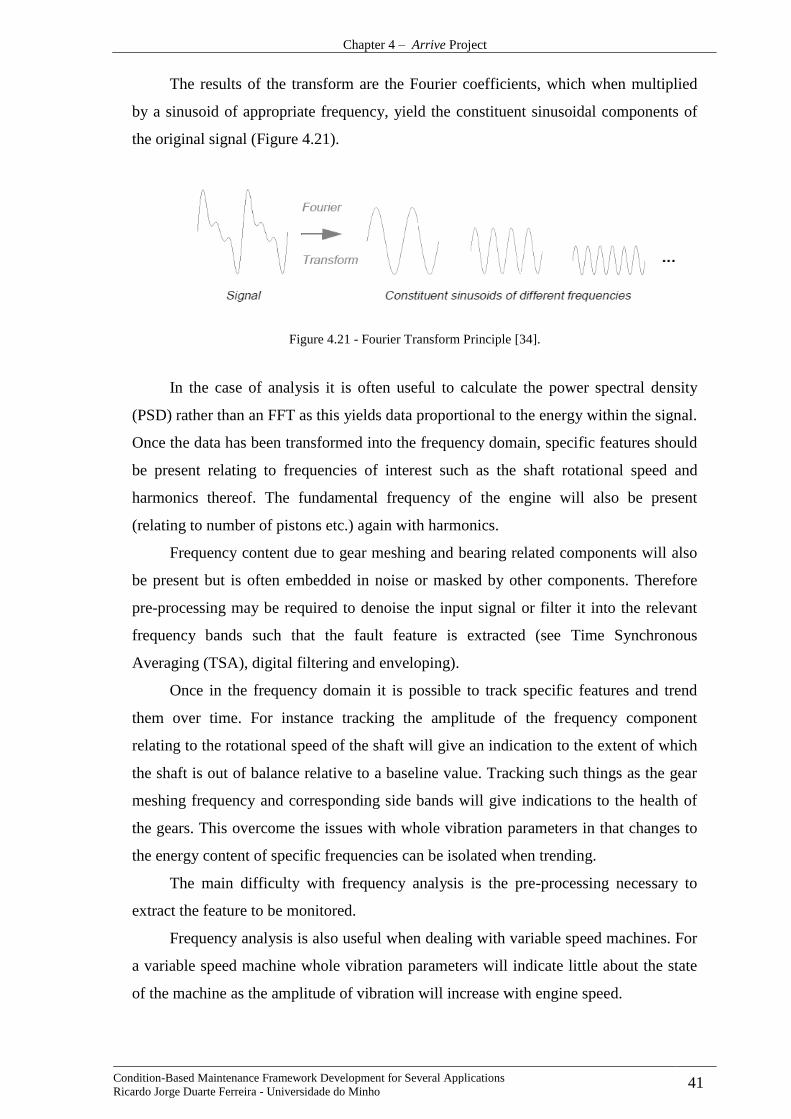
Chapter 4 – Arrive Project
Condition-Based Maintenance Framework Development for Several Applications 41 Ricardo Jorge Duarte Ferreira - Universidade do Minho
The results of the transform are the Fourier coefficients, which when multiplied
by a sinusoid of appropriate frequency, yield the constituent sinusoidal components of
the original signal (Figure 4.21).
Figure 4.21 - Fourier Transform Principle [34].
In the case of analysis it is often useful to calculate the power spectral density
(PSD) rather than an FFT as this yields data proportional to the energy within the signal.
Once the data has been transformed into the frequency domain, specific features should
be present relating to frequencies of interest such as the shaft rotational speed and
harmonics thereof. The fundamental frequency of the engine will also be present
(relating to number of pistons etc.) again with harmonics.
Frequency content due to gear meshing and bearing related components will also
be present but is often embedded in noise or masked by other components. Therefore
pre-processing may be required to denoise the input signal or filter it into the relevant
frequency bands such that the fault feature is extracted (see Time Synchronous
Averaging (TSA), digital filtering and enveloping).
Once in the frequency domain it is possible to track specific features and trend
them over time. For instance tracking the amplitude of the frequency component
relating to the rotational speed of the shaft will give an indication to the extent of which
the shaft is out of balance relative to a baseline value. Tracking such things as the gear
meshing frequency and corresponding side bands will give indications to the health of
the gears. This overcome the issues with whole vibration parameters in that changes to
the energy content of specific frequencies can be isolated when trending.
The main difficulty with frequency analysis is the pre-processing necessary to
extract the feature to be monitored.
Frequency analysis is also useful when dealing with variable speed machines. For
a variable speed machine whole vibration parameters will indicate little about the state
of the machine as the amplitude of vibration will increase with engine speed.

Chapter 4 – Arrive Project
42 Condition-Based Maintenance Framework Development for Several Applications
Ricardo Jorge Duarte Ferreira - Universidade do Minho
4.3.2.2. Wavelet Transform
Compare wavelets with sine waves, which are the basis of Fourier analysis.
Sinusoids do not have limited duration —they extend from minus to plus infinity. And
where sinusoids are smooth and predictable, wavelets tend to be irregular and
asymmetric (Figure 4.22).
Figure 4.22 - Comparison between a Sine Wave and a Wavelet [32].
Fourier analysis consists of breaking up a signal into sine waves of various
frequencies. Similarly, wavelet analysis is the breaking up of a signal into shifted and
scaled versions of the original (or mother) wavelet.
A wavelet is a waveform of effectively limited duration that has an average value
of zero.
Just looking at pictures of wavelets and sine waves, you can see intuitively that
signals with sharp changes might be better analyzed with an irregular wavelet than with
a smooth sinusoid. It also makes sense that local features can be described better with
wavelets, which have local extent.
Similarly to the FFT, the continuous wavelet transform (CWT) is defined as the
sum over all time of the signal multiplied by scaled, shifted versions of the
wavelet function Ψ:
The result of the CWT is many wavelet coefficients C, which are a function of
scale and position (Figure 4.23).

Chapter 4 – Arrive Project
Condition-Based Maintenance Framework Development for Several Applications 43 Ricardo Jorge Duarte Ferreira - Universidade do Minho
Figure 4.23 - Wavelet Transform Principle [32].
This process can be resumed in 5 steps described below:
1. Take a wavelet and compare it to a section at the start of the original signal.
2. Calculate a number, C, that represents how closely correlated the wavelet is
with this section of the signal. The higher C is, the more the similarity. Note
that the results will depend on the shape of the chosen wavelet (Figure 4.24).
Figure 4.24 – 2nd
step of Wavelet Transform Algorithm [32].
3. Shift the wavelet to the right and repeat steps 1 and 2 until covering the
whole signal (Figure 4.25).
Figure 4.25 – 3rd
step of Wavelet Transform Algorithm [32].
4. Scale (stretch) the wavelet and repeat steps 1 through 3 (Figure 4.26).

Chapter 4 – Arrive Project
44 Condition-Based Maintenance Framework Development for Several Applications
Ricardo Jorge Duarte Ferreira - Universidade do Minho
Figure 4.26 – 4th
step of Wavelet Transform Algorithm [32].
5. Repeat steps 1 through 4 for all desired scales.
As described, the continuous wavelet transform is the sum over all time of the
signal multiplied by scaled, shifted versions of the wavelet. This process produces
wavelet coefficients that are a function of scale and position.
In the end coefficients at different scales by different sections of the signal are
produced. The coefficients constitute the results of a regression of the original signal
performed on the wavelets. A common approach to make sense of this coefficients is to
plot them using x-axis representing position along the signal (time), the y-axis
representing scale, and the color at each x-y point represents the magnitude of the
wavelet coefficient C (Figure 4.27).
Figure 4.27 – 2d Plot of Continuous Wavelet Transform [32].
3d plots are also another option to visualize the Continuous Wavelet Transform
(Figure 4.28).
The continuous wavelet transform coefficient plots are precisely the time-scale
view of the signal processed. It is a different view of signal data than the time-frequency
Fourier view, but it is not unrelated.

Chapter 4 – Arrive Project
Condition-Based Maintenance Framework Development for Several Applications 45 Ricardo Jorge Duarte Ferreira - Universidade do Minho
Figure 4.28 –3d Surface Plot of Continuous Wavelet Transform [32].
4.3.2.2.1. Wavelet Transform
As seen in Figure 4.27, y-axis labels run from 1 to 31. Recall that the higher
scales correspond to the most “stretched” wavelets. The more stretched the wavelet, the
longer the portion of the signal with which it is being compared, and thus the coarser the
signal features being measured by the wavelet coefficients.
Thus, there is a correspondence between wavelet scales and frequency as revealed
by wavelet analysis:
Thus, there is a correspondence between wavelet scales and frequency as revealed by
wavelet analysis:
Low scale a Compressed wavelet
Rapidly changing details
High frequency ω.
High scale a Stretched wavelet
Slowly changing, coarse features
Low frequency ω.
The fact that wavelet analysis does not produce a time-frequency view of a signal
is the strength of the technique. Not only is time-scale a different way to view data, it is
a very natural way to view data deriving from a great number of natural phenomena.

Chapter 4 – Arrive Project
46 Condition-Based Maintenance Framework Development for Several Applications
Ricardo Jorge Duarte Ferreira - Universidade do Minho
4.3.2.2.2. One-Stage Filtering: Approximations and Details
For many signals, the low-frequency content is the most important part. It is what
gives the signal its identity. The high-frequency content, on the other hand, imparts the
details. Consider the human voice. If the high-frequency components are removed, the
voice sounds different, but is still possible to tell what’s being said. However, if enough
of the low-frequency components are removed, gibberish is heard. It is for this reason
that, in wavelet analysis, often refers to the terms of approximations and details.
The approximations are the high-scale, low-frequency components of the signal.
The details are the low-scale, high-frequency components. The filtering process, at its
most basic level is presented in Figure 4.29.
Figure 4.29 - One-Stage Filtering schematic [32].
The original signal, S, passes through two complementary filters and emerges as
two signals.
Unfortunately, when actually performing this operation on a real digital signal,
twice as much data as started is generated. Suppose, for instance, that the original signal
S consists of 1000 samples of data. Then the approximation and the detail will each
have 1000 samples, for a total of 2000 (Figure 4.30).
Figure 4.30 - One-Stage Wavelet Filtering schematic [32].

Chapter 4 – Arrive Project
Condition-Based Maintenance Framework Development for Several Applications 47 Ricardo Jorge Duarte Ferreira - Universidade do Minho
The process on the right, which includes down sampling, produces DWT
coefficients. To gain a better appreciation of this process, a one-stage discrete wavelet
transform of a signal will be presented. The used signal will be a pure sinusoid with
high-frequency noise added to it.
Using the following code on matlab:
s = sin(20.*linspace(0,pi,1000)) + 0.5.*rand(1,1000);
[cA,cD] = dwt(s,'db2');
The schematic of the process will be shown in Figure 4.31.
Figure 4.31 – One-Stage Wavelet Filtering example [32].
Notice that the detail coefficients cD consist mainly of the high-frequency noise,
while the approximation coefficients cA contain much less noise than does the original
signal.
It may observe that the actual lengths of the detail and approximation coefficient
vectors are slightly more than half the length of the original signal.
This has to do with the filtering process, which is implemented by convolving the
signal with a filter. The convolution “smears” the signal, introducing several extra
samples into the result.
4.3.2.2.3. Multi-Level Decomposition
The decomposition process can be iterated, with successive approximations being
decomposed in turn, so that one signal is broken down into many lower-resolution
components. This is called the wavelet decomposition tree (Figure 4.32).

Chapter 4 – Arrive Project
48 Condition-Based Maintenance Framework Development for Several Applications
Ricardo Jorge Duarte Ferreira - Universidade do Minho
Figure 4.32 - Multi-Level Decomposition Schematic [32].
4.3.2.2.4. Wavelet Reconstruction
It has been shown how the discrete wavelet transform can be used to analyze, or
decompose, signals and images. Another useful concept is how those components can
be assembled back into the original signal with no loss of information. This process is
called inverse discrete wavelet transforms (IDWT) (Figure 4.33).
Figure 4.33 – Inverse Discrete Wavelet Transform schematic [32].
Where wavelet analysis involves filtering and down-sampling, the wavelet
reconstruction process consists of up-sampling and filtering. Up-sampling is the process
of lengthening a signal component by inserting zeros between samples (Figure 4.34).
Figure 4.34 – Up-sampling step used on IDWT [32].

Chapter 4 – Arrive Project
Condition-Based Maintenance Framework Development for Several Applications 49 Ricardo Jorge Duarte Ferreira - Universidade do Minho
This process is mandatory in order to analyze the signal using FFT as will be
presented in the next chapter.

50 Condition-Based Maintenance Framework Development for Several Applications
Ricardo Jorge Duarte Ferreira - Universidade do Minho
CHAPTER 5
Implemented Algorithms and C# Libraries
Introduction 5.1.
All the following algorithms were developed in matlab and then compiled to C#
and deployed in a web service that performs the calculation of the algorithms every time
new data is available. The proposed algorithms were developed based in reviews of
recent research of vibration techniques for various types of rotating machinery stated by
literature. Also matlab was opted as main algorithms development based platform
because is the standard platform used for these applications, ease of use, and internal
knowledge that the company already have in this environment.
The method used for running the matlab code in a C# environment is the matlab
Compiler Runtime (MCR) which enables royalty-free deployment to users who do not
have matlab.
It is possible to package the MCR with the developed application or have your
users download it during installation.
To compile the matlab code to C#, though, it is necessary to have the matlab
Compiler that compiles the libraries and applications that then can be used in C#. A
detailed guide on how to compile matlab code to C# can be found in [35].
Signal Generator 5.2.
The performance of the implemented methods is demonstrated using a computer–
generated simulated signal [15]. The signal was built with a sampling frequency of 8
kHz. The major components include a 60/(Simulated Speed) Hz component considered
as slow shaft relative amplitude 1.0, 30/(Simulated Speed) Hz fast shaft (relative
amplitude 0.6), 34/(Simulated Speed) Hz gear meshing frequency relative amplitude
0.3, and a 10/(Simulated Speed) Hz characteristic frequency, carried on a modulated 2.0
kHz wave, with a random jitter (max. 3%), simulating for instance a rolling–element–
bearing outer race fault; the signal has initial amplitude of 0.1, decaying with a time
constant of 2 ms.
The referred signal is presented in Figure 5.1.

Chapter 5 – Implemented Algorithms and C# Libraries
51 Condition-Based Maintenance Framework Development for Several Applications
Ricardo Jorge Duarte Ferreira - Universidade do Minho
Also a signal considered as a good condition signal was used which consisted in
changing the Rolling Element component to only a 10/(Simulated Speed) Hz
characteristic frequency (Figure 5.2).
In the end summing all the compositions of the signal components shown in
Figure 5.1 the signal presented in Figure 5.3 is achieved.
Figure 5.1 - Simulated faulty signal using matlab for Input “(Simulated Speed)” = 1500 rpm.
Figure 5.2 -- Simulated good signal using matlab for Input “(Simulated Speed)” = 1500 rpm.

Chapter 5 – Implemented Algorithms and C# Libraries
52 Condition-Based Maintenance Framework Development for Several Applications
Ricardo Jorge Duarte Ferreira - Universidade do Minho
Figure 5.3 - Overall Signal with Faulty Bearing Components.
These simulated functions can be generated in matlab using the function:
[t,YGood, YFaulty, Fs]=Generate((Simulated Speed));
In which is the referred “(Simulated Speed)” is the value correspondent to the
desired Simulated Speed.
In C# by adding the reference “GenerateSignals.dll” to the project and adding the
following lines to the code:
// Initialize GenerateSignals
GenerateSignals.BearingFault SignalObj = new GenerateSignals.BearingFault(); //Generate Simulated Signals double Speed = 1500; //Speed of Motor SignalClass Signal = new SignalClass( SignalObj.Generate(4, Speed)); //Call Matlab Function to generate signals
Signal Class was created to help handling the values and consists in a simple
class:
public class SignalClass { public MWArray t; public MWArray YGood; public MWArray YFaulty; public MWArray Fs; public SignalClass(MWArray[] MWArray) { t = MWArray[0]; YGood = MWArray[1]; YFaulty = MWArray[2]; Fs = MWArray[3]; }

Chapter 5 – Implemented Algorithms and C# Libraries
Condition-Based Maintenance Framework Development for Several Applications 53 Ricardo Jorge Duarte Ferreira - Universidade do Minho
Indicators 5.3.
As shown in “Statistical parameters” section, there are several Time based
Indicators that can be used in Condition Monitoring. For the presented project some
indicators were implemented and the library for using those Indicators in a C# project
was generated.
On matlab environment following (assumed that the signal was simulated with the
previous function), the developed indicators can be calculated as shown:
%Calculate Mean of Signal Mean = mean(YSignal); %Calculate Crest Factor of Signal CrestFactor = crest(YSignal); %Calculate Kurtoisis of Signal Kurtosis = kurtosis(YSignal); %Calculate Standard Deviation of Signal Std = std(YSignal); %Calculate Variance of Signal Var = var(YSignal); %Calculate Mean and Standard Deviation of Peak 2 Peak frame = Speed/60; YFaulty.meanp2p = meanp2p(YSignal, frame, Fs); YFaulty.stdp2p = stdp2p(YSignal, frame, Fs);
A small description can be added on this last function “meanp2p” and “stdp2p”.
To calculate the value of the Mean Peak to Peak, as input is needed the desired frame of
the signal, which an example can be the Speed / 60 (which will give the Fundamental
Component Mean Peak to Peak) and the Signal Frequency. With this the Peak to Peak
value in the desired frame can be calculated and also the Standard Deviation of the
Peaks.
For the Simulated Signal at the Speed of 1500 rpm the detected peaks are shown
in Figure 5.4 and Figure 5.5.

Chapter 5 – Implemented Algorithms and C# Libraries
54 Condition-Based Maintenance Framework Development for Several Applications
Ricardo Jorge Duarte Ferreira - Universidade do Minho
Figure 5.4 - Graphic of Mean Peak to Peak Calculation.
Figure 5.5 - Histogram of Mean Peak to Peak Calculation.
Using this, the mean value of peak to peak and the standard deviation are
calculated.
In C# by adding the reference “Indicators.dll” to the project and adding the
following lines to the code, the algorithms can be calculated.
// Initialize Indicators IndicatorClass Indicators = new IndicatorClass();//Generate Simulated Signals var Mean = IndObj.mean(YSignal); var CrestFactor = IndObj.crest(YSignal); var Kurtosis = IndObj.kurtosis(YSignal); var Std = IndObj.std(YSignal); var Var = IndObj.var(YSignal); var Meanp2p = IndObj.meanp2p(YSignal, Speed/60, Fs); var Stdp2p = IndObj.stdp2p(YSignal, Speed/60, Fs);
Complex Functions 5.4.
Theory behind the implemented complex functions is presented in several
chapters of the section “Signal processing”.
Fast Fourier Transform and Peak Detection 5.5.
FFT function can be called from matlab using the following command:
[time, power, FFTMax, PowerMax]=FFT(YSignal, Fs);

Chapter 5 – Implemented Algorithms and C# Libraries
Condition-Based Maintenance Framework Development for Several Applications 55 Ricardo Jorge Duarte Ferreira - Universidade do Minho
FFT when used with “LocatePeaks” is a powerful tool. After using FFT, user can
use the “LocatePeaks” function in order to take information of the Peaks found in the
FFT.
As there is some noise within the FFT is necessary to use Thresholds in order to
minimize the information returned by the function “LocatePeaks”. These Thresholds
were manually chosen and may/should be changed when applied on a real application.
To use the function “LocatePeaks” the user is asked to use 3 parameters:
Threshold - Minimum height difference. Specify the threshold height
difference between a peak and its neighboring values as a positive real
number. “LocatePeaks” only returns peaks that exceed their neighbors by
at least the value of the Threshold.
MinPeakHeight - Minimum peak height. Specify the minimum peak
height as a real-valued scalar. “LocatePeaks” only returns peaks that
exceed the MinPeakHeight.
MinPeakDistance - Minimum peak separation. Specify the minimum
peak distance, or minimum separation between peaks as a positive integer.
User can use the MinPeakDistance option to specify that the algorithm
ignore small peaks that occur in the neighborhood of a larger peak. When
user specifies a value for MinPeakDistance, the algorithm initially
identifies all the peaks in the input data and sorts those peaks in
descending order. Beginning with the largest peak, the algorithm ignores
all identified peaks not separated by more than the value of
MinPeakDistance.
One example of implementation after previous using FFT can be:
%Defining the parameters Threshold = 0.00001; MinPeakHeight = FFTMax*0.0000001; MinPeakDistance = 10; %Find Peaks [Xpeaks, Ypeaks] = LocatePeaks(YSignal, Threshould, MinPeakHeight, MinPeakDistance);
For the implement simulated function using Speed = 1500 rpm, the output of this
function for the faulty signal and good signal is shown in Figure 5.6 respectively.

Chapter 5 – Implemented Algorithms and C# Libraries
56 Condition-Based Maintenance Framework Development for Several Applications
Ricardo Jorge Duarte Ferreira - Universidade do Minho
As expected the “Good Signal” don’t present the high frequency components that
are seen in the “Faulty Signal” and presents much less harmonics. This is due to the
complexity of the Bearing Faulty Simulated Signal.
Also adding the reference “ComplexFunctions.dll” to the project and adding the
following lines to the code, the algorithms can be calculated.
//Inicialize Complex Functions ComplexFunctions.ComplexFunctions CompFunctObj = new ComplexFunctions.ComplexFunctions(); //Calculate FFT var FFT = CompFunctObj.FFT(4, YSignal, Fs); //Find FFT Peaks MWArray Threshould = 0.000001; MWArray MinPeakHeight = FFT[2] * 0.0001; MWArray MinPeakDistance = 1; var FFTPeaks = CompFunctObj.LocatePeaks(2, FFT[0], FFT[1], Threshould, MinPeakHeight, MinPeakDistance);
Figure 5.6 - On top picture FFT of “Faulty Signal” is shown and on bottom picture FFT of “Good Signal”
is shown.

Chapter 5 – Implemented Algorithms and C# Libraries
Condition-Based Maintenance Framework Development for Several Applications 57 Ricardo Jorge Duarte Ferreira - Universidade do Minho
Filtering 5.6.
The implemented filter consists in a Butterworth Filter. This filter is implemented
in a two-step process using the following functions:
%Constructing the Filter [a,b]=butter(order,Wn,ftype); %Applying the filter to the signal Signal = filter(a,b,Signal);
Where:
order – Order of the filter;
Wn – Is the cut-off frequency of the filter which is a value if ftype is
“high” or “low” or a vector if ftype is “stop” or ”bandpass”.
Ftype – Is the type of filtering implemented and can be: “high”, “low”,
“stop” or “bandpass”.
The stop band and the band pass filters were used. One example of
implementation can be:
FreqBand = 200; %Window for the filter CutOffFrequency = 2000 %Wanted Cutt-Off Frequency WnS = ((CutOffFrequency+FreqBand)/(Fs/2)); %Lower Limit for the Filter WnI = ((CutOffFrequency-FreqBand)/(Fs/2)); %Upper Limit for the Filter %Construction of the Frequency Vector Wn =[WnI WnS] %Filter Band Signal [a,b]=butter(15,Wn,'bandpass'); PassBandSignal = filter(a,b,YFaulty); %High pass Filter [a,b]=butter(15,Wn,'stop'); StopBandSignal = filter(a,b,YFaulty);
For the implement simulated function using Speed = 1500, the output of this
function for the Faulty Signal using has input of the filter the Faulty Frequency of 2000
Hz (Figure 5.7).

Chapter 5 – Implemented Algorithms and C# Libraries
58 Condition-Based Maintenance Framework Development for Several Applications
Ricardo Jorge Duarte Ferreira - Universidade do Minho
Figure 5.7 – Output of Butterworth Filter applied to Faulty Signal using as input 2000 Hz Cut-Off
Frequency.
It is possible to see that the filtering can actually take valuable information about
the Faulty Frequency. If “FFT” is on filtered signals, the effectiveness of the
implemented filter can be seen and is shown in Figure 5.8.
Figure 5.8 – FFT on Filtered Signals.
Clearly is seen that filter Cut-Off slope is very high. That is due to the selected
order of the filter of 15. If a lower order filter was chosen the filter wasn’t so accurate.
Also in “ComplexFunctions.dll” library, the Filtering functionality can be used in
the project by adding the following lines to the code:

Chapter 5 – Implemented Algorithms and C# Libraries
Condition-Based Maintenance Framework Development for Several Applications 59 Ricardo Jorge Duarte Ferreira - Universidade do Minho
//BandPass Signal using Butterworth Filter with frequency 2000Hz
double[] aux = new double[2] { 2.00 * 2000 / Fs * 0.90, 2.00 * 2000 / Fs * 1.10 }; MWNumericArray Wn = new MWNumericArray(aux); MWArray FilterOrder = 15; //Order of the filter MWArray FilterType = "bandpass"; //Band pass type filter //Create Butterworth Filter MWArray[] Filter = CompFunctObj.butter(2, FilterOrder, Wn, FilterType); //Apply BandPass Filter to Signal MWArray PassFreqSignal = CompFunctObj.filter(Filter[0], Filter[1], YSignal); FilteredSignalPassComp = ConvertToDouble(HighFreqSignal); //Apply StopBand Filter to the Signal using same Filter FilterType = "stop"; //Band pass type filter //Apply Filter to Signal MWArray StopFreqSignal = CompFunctObj.filter(Filter[0], Filter[1], YSignal);
FilteredSignalStopComp = ConvertToDouble(StopFreqSignal);
Enveloping 5.7.
There are some techniques regarding Signal Enveloping. One of the easiest one
and implemented using the function “envelop” basically consisted in reutilizing some
parts of the code used for the calculation of the EMD imfs. It consists on a two-step
process:
Identify local maxima;
Deduce an upper interpolation (cubic splines);
The “envelop” function is called using the following command:
envelopSignal = envelop(Signal);
In comparison to this simple Enveloping technique, a more complex approach
described in the literature was also used, the “Hilbert Envelop” and can be called using
the function “hilbertenvelop”.
The “hilbertenvelop” function is called using the following command:
HilbertSignal = hilbertenvelop(PassBandSignal);
Using this simple enveloping in the Stop Band Filtered Signal is a good
application of this kind of enveloping and the result is shown in Figure 5.9.

Chapter 5 – Implemented Algorithms and C# Libraries
60 Condition-Based Maintenance Framework Development for Several Applications
Ricardo Jorge Duarte Ferreira - Universidade do Minho
Figure 5.9 – Simple Enveloping and Hilbert Enveloping applied to the Stop Band Filtered Signal.
Using the FFT on the Envelop Signals, some new unknown information about the
signal can be seen.
In Figure 5.10 the FFT of the Simple Enveloping and of the Hilbert Enveloping is
presented.
Both Enveloping techniques detect a peak at 195 Hz which clearly is a signature
of the Faulty Bearing Component. The Hilbert Enveloping also shows a peak at higher
frequency but possible this has another interpretation that was not studied in enough
detail to take conclusions.
Figure 5.10 – Signal eveloping using “envelop” function(Red) and using “hilbertenvelop” function
(Black).

Chapter 5 – Implemented Algorithms and C# Libraries
Condition-Based Maintenance Framework Development for Several Applications 61 Ricardo Jorge Duarte Ferreira - Universidade do Minho
Both this enveloping techniques are available in the “ComplexFunctions.dll”
library:
//Envelop Signal MWArray Envelop = CompFunctObj.envelop(YSignal); //Envelop Signal MWArray HilbertEnvelop = CompFunctObj.hilbertenvelop(YSignal);
Empiricial Mode Decomposition 5.8.
EMD can be considered a more complex Enveloping technique as described in the
“Technical Details” Section. The EMD generates on its outputs the called imfs that
contain information about several frequency components on a signal. The EMD
function can be used on matlab like the example shown:
%Calculate Signal Empirical Mode Decomposition imf = EMD(YSignal);
Using this EMD function all the imfs are calculated, and an example using the
Faulty Signal shown in Figure 5.11.
It is clearly seen that the Imfs shows valuable information about the signal. As
usual the EMD can then be combined with the FFT to examine the predominant
frequency component on each the Imf and will be obtained result will be shown on
Figure 5.12.

Chapter 5 – Implemented Algorithms and C# Libraries
62 Condition-Based Maintenance Framework Development for Several Applications
Ricardo Jorge Duarte Ferreira - Universidade do Minho
Figure 5.11 –Imfs(Blue) and Simple Enveloping(Red) on Faulty Signal.

Chapter 5 – Implemented Algorithms and C# Libraries
Condition-Based Maintenance Framework Development for Several Applications 63 Ricardo Jorge Duarte Ferreira - Universidade do Minho
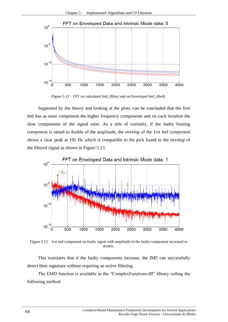
Chapter 5 – Implemented Algorithms and C# Libraries
64 Condition-Based Maintenance Framework Development for Several Applications
Ricardo Jorge Duarte Ferreira - Universidade do Minho
Figure 5.12 – FFT on calculated Imfs (Blue) and on Enveloped Imfs (Red).
Supported by the theory and looking at the plots, can be concluded that the first
Imf has as main component the higher frequency components and on each iteration the
slow components of the signal raise. As a title of curiosity, if the faulty bearing
component is raised to double of the amplitude, the envelop of the 1rst Imf component
shows a clear peak at 195 Hz which is compatible to the pick found in the envelop of
the filtered signal as shown in Figure 5.13.
Figure 5.13 – 1rst imf component on faulty signal with amplitude of the faulty component increased to
double.
This translates that if the faulty components increase, the IMF can successfully
detect their signature without requiring an active filtering.
The EMD function is available in the “ComplexFunctions.dll” library calling the
following method:

Chapter 5 – Implemented Algorithms and C# Libraries
Condition-Based Maintenance Framework Development for Several Applications 65 Ricardo Jorge Duarte Ferreira - Universidade do Minho
//Envelop Signal MWArray Imfs = CompFunctObj.EMD(YSignal);
Time Synchronous Averaging 5.9.
TSA is a technique that is very used and known throw the literature.
Unfortunately at the time of the creation of this report, only simulated data was used so
no trigger from a tachometer was provided. This means that another approach was used.
On matlab environment, when calling the function “TSA”, the user needs to use the
following function:
%Perfom time Syncronous Average base on Fundamental frequency input frame = Speed/60; [Time,SyncronousSignals]=tsa(YSignal, frame, Fs);
Basically this inputs consist in the same as the ones used for the calculation of the
Mean Peak to Peak. The output of this function is a vector of time and another with all
the detected synchronous signals. In the case of our faulty signal, the output of this
function can be seen on Figure 5.14.
Figure 5.14 – Detected Synchronous Signals using TSA function on Faulty Signal.
A common approach now would be calculating the mean signal of all the
synchronous signals. This is easily achieved with the simple command:
%Calculate mean of Syncronous Signals TSaSignal = mean(SyncronousSignals);
The result of this function can be seen on Figure 5.15.

Chapter 5 – Implemented Algorithms and C# Libraries
66 Condition-Based Maintenance Framework Development for Several Applications
Ricardo Jorge Duarte Ferreira - Universidade do Minho
Figure 5.15 – Time Synchronous Averaged Signal.
Again, the user can has now some options to use this signal. A common procedure
is to calculate the indicators on the Time Synchronous Averaged Signal and monitor
them over time. It is also possible to calculate the FFT and detect the peaks of this
Signal (Figure 5.16).
Figure 5.16 – FFT on Time Synchronous Averaged Signal.
Clearly this FFT has less noise that the raw Signal as expected.
Another approach can be applying the so called Short Time Fast Fourier
Transform using each of the Detected Synchronous signals. Using the vector of the
Synchronous Signals a simple code to calculate the Short Time Fast Fourier Transform.
This function output is shown in Figure 5.17.
%Calculate Short Time Fast Fourier [Timer,Power,Count]= STFFT(Time,SyncronousSignals, Fs);

Chapter 5 – Implemented Algorithms and C# Libraries
Condition-Based Maintenance Framework Development for Several Applications 67 Ricardo Jorge Duarte Ferreira - Universidade do Minho
%Plot the result plot3(Timer, Count, Power);
This is implemented and is possible for the user to use this function. Still more
study needs to be done in order to validate the possibility of the extraction of some
valuable indicators from output of this function.
All the referred functions are also implemented in the “ComplexFunctions.dll”
library as shown below:
//Calculate Time Synchronous Averaging
MWNumericArray frame = new MWNumericArray(Speed / 60);
MWArray[] TSA = CompFunctObj.tsa(2,Signal, frame, Fs);
//Mean value of TSA signal
Indicators.Indicators IndObj = new Indicators.Indicators();
MWArray TSASignal = IndObj.mean(TSA[1]);
//FFT of Tsa Signal
MWArray[] TSA_FFT = CompFunctObj.FFT(4, TSASignal, Fs);
//STFFT of Tsa Signal
MWArray[] TSA_STFFT =CompFunctObj.STFFT(3, TSA[0], TSA[1]);
Figure 5.17 – Short Time Fast Fourier on Detected Synchronous signals.
Wavelet Decomposition 5.10.
Wavelet Decomposition is a powerful algorithm vastly described in the literature.
One implemented function based on this concept is “WaveletDecomposition” and it can
be used like shown below:
%Define Wavelet wname ='db8'; DecompositionNumber =5;

Chapter 5 – Implemented Algorithms and C# Libraries
68 Condition-Based Maintenance Framework Development for Several Applications
Ricardo Jorge Duarte Ferreira - Universidade do Minho
%Define Wavelet Decomposition [Time,LowFreq, HighFreq, Fs]=WaveletDecomposition(Ysignal, Fs, wname, DecompositionNumber);
The output of this function can then be plotted and is show in Figure 5.18.
Figure 5.18 –Wavelet Decomposition on Faulty Signal (Blue) and Simple Enveloping Signal (Red).
Notice that in the plots shown above, the x-axis refer to sample number. Each
time a wavelet decomposition is made the number of samples decrease. This results in a

Chapter 5 – Implemented Algorithms and C# Libraries
Condition-Based Maintenance Framework Development for Several Applications 69 Ricardo Jorge Duarte Ferreira - Universidade do Minho
lower sample rate meaning that a correction needs to be done in the sampling rate in
order to calculate the FFT.
As expected each decomposition acts like a filter on the signal. FFT can then be
calculated to take some conclusions (Figure 5.19).
Figure 5.19 – FFT on Wavelet decomposition (Blue) and Simple Enveloping Signal (Red).
Using FFT on the Wavelet decomposition signals a very important conclusion
could be taken. Looking to the FFT on the High Frequency Decomposition 1, we can

Chapter 5 – Implemented Algorithms and C# Libraries
70 Condition-Based Maintenance Framework Development for Several Applications
Ricardo Jorge Duarte Ferreira - Universidade do Minho
see that the Higher Peak is the Peak close to the Faulty Bearing. Also the envelop peak
shows a similar signature to the Faulty Bearing.
Whoever, has the sampling rate was decrease by half when performing wavelet
decomposition (from 8000 Hz of the original signal to 4000 Hz), there was not enough
sampling rate to successfully detected the exact frequency of the faulty signal. To prove
this theory the sampling rate of the original signal was increased from 8000 Hz to 10
000 Hz and the results are presented on Figure 5.20:
Figure 5.20 - FFT on Wavelet decomposition (Blue) and Simple Enveloping Signal (Red).

Chapter 5 – Implemented Algorithms and C# Libraries
Condition-Based Maintenance Framework Development for Several Applications 71 Ricardo Jorge Duarte Ferreira - Universidade do Minho
With the increase of the original signal, it can be seen that High Frequency
Decomposition 1, successfully detected a Peak corresponding to the Faulty Bearing
proving also that a sample rate limitation was causing the frequency distortion. Also the
envelop peak keeps showing a similar signature to the Faulty Bearing.
In some applications increasing the Sampling Rate can have big drawbacks and
sometimes also mean buying an expensive Acquisitions Systems. Some research was
made around the possible solutions regarding this problem and it was discovered that
using Inverse Wavelet on the Decomposed Signals restored the Sampling rate on the
Signals. This was implemented using the function
“WaveletDecompositionWithReconstruction”.
%Define Wavelet wname ='db8'; DecompositionNumber =5;
%Define Wavelet Decomposition with Reconstruction [LowFreq, HighFreq]=WaveletDecompositionWithReconstruction(Ysignal, wname, DecompositionNumber);
The output of this function can be seen in Figure 5.21.

Chapter 5 – Implemented Algorithms and C# Libraries
72 Condition-Based Maintenance Framework Development for Several Applications
Ricardo Jorge Duarte Ferreira - Universidade do Minho
Figure 5.21 –Wavelet Decomposition on Faulty Signal (Blue) and Simple Enveloping Signal (Red).
As expected each decomposition acts like a filter on the signal. FFT can then be
calculated to take some conclusions (Figure 5.22).

Chapter 5 – Implemented Algorithms and C# Libraries
Condition-Based Maintenance Framework Development for Several Applications 73 Ricardo Jorge Duarte Ferreira - Universidade do Minho
Figure 5.22 – FFT on Wavelet decomposition (Blue) and Simple Enveloping Signal (Red).
Using FFT on the Wavelet Decomposition with Reconstruction signals, a very
important conclusion could be taken. Looking to the FFT on the High Frequency
Decomposition 1, we can see that the Higher Peak is the Peak characteristic of the
Faulty Bearing. Also the envelop peak shows a similar signature to the Faulty Bearing.
This means that this technique can be used for diagnosis which makes this functionality
very interesting.
Wavelet Decomposition with Reconstruction is also accessible using
“ComplexFunctions.dll” library as shown below:
//Wavelet Decomposition with Reconstruction MWArray wname = "db8"; MWArray DecompositionNumber = 5; MWArray[] WaveDec = CompFunctObj.WaveletDecompositionWithReconstruction(2, YSignal, wname, DecompositionNumber);
Continuous Wavelet Transform, referred in “Signal processing” of this report, was
also implemented during this work. It is a very complex function not a lot of interest
was given to it whoever for further studies /applications this technique can be useful
and is also worthy to talk about in this document. This function can be accessed on
matlab using the function “ContinuousWaveletTransform” like shown in the example
below:
%Calculate Continuos Wavelet Transform [wave, period, scale, coi, dj,paramout, k] = ContinuousWaveletTransform (YSignal, Fs);
After that the result can be plotted on 2d like the following example:

Chapter 5 – Implemented Algorithms and C# Libraries
74 Condition-Based Maintenance Framework Development for Several Applications
Ricardo Jorge Duarte Ferreira - Universidade do Minho
freq = 1./period; power = abs(wave).^2; contour(t,freq,log(power));
Figure 5.23 – Continuous Wavelet Transform on Faulty Signal.
Figure 5.24 – Continuous Wavelet Transform on Good Signal.
It can be seen that the Continuous Wavelet Transform on Faulty Signal (Figure
5.23) shows higher Power Spectrum on High Frequencies than the Continuous Wavelet
Transform on Good Signal (Figure 5.24). Whoever as this signals are continuous this
algorithm suits better to detect any discontinuity has referred.
Diagnoses Library 5.11.
The diagnoses library consists in a web service that can be deployed on a server
and remains waiting for receiving a OSA-CBM request that is sent using the scheduler
every time the a job is created in the database.

Chapter 5 – Implemented Algorithms and C# Libraries
Condition-Based Maintenance Framework Development for Several Applications 75 Ricardo Jorge Duarte Ferreira - Universidade do Minho
Basically this web service consist in calculate all the developed algorithms on the
triggered signal and send the obtained values to the database using OSA-CBM interface.
A basic flowchart of the implemented algorithm is shown in Figure 5.25.
Figure 5.25 – FlowChart of the diagnoses library.

76 Condition-Based Maintenance Framework Development for Several Applications
Ricardo Jorge Duarte Ferreira - Universidade do Minho
CHAPTER 6
Conclusions
In this work, several the work performed during the Internship in Critical
Software Technologies is presented. In a first approach was needed to understand the
problems that a CBM system tries to solve and it’s place in modern industry. That was
presented in Chapter 1 and developed in detail in Chapter 2 contextualizing with other
common approaches for maintenance.
In Chapter 3, is presented a system for train conditioning-based monitoring that
was improved during this internship and it’s features. Through the work in this project,
knowledge related to key components of a train and common measures on a system was
developed and a framework where is possible to test all the features of a conditioning
monitoring system is presented.
Chapter 4 presents the work done for Arrive project. This project is very recent
and aims to monitor rotational machines present health indicators regarding assets
condition. The developments on this project were done slowly because most of the
improvements were firstly done in Alstom and then adapted. Here firstly insights on
common faults were studied and common approaches suggested by the literature are
presented.
Chapter 5 finally presents the results obtained with the developed algorithms.
Although the code is not presented, it is intended for this chapter to be a starting point
for anyone who wants to develop algorithms for CBM systems.
The environment developed by Critical Software Technologies regarding
conditioning-based monitoring system is a very powerful framework. The overall
architecture is made in a way that is easily adaptable to other applications. At this points
more work needs to be done in order to build a truly adaptable structure that lower the
costs in terms of future developments to become more compatible in the field.
In order to prove the concept for both the framework and applicability in vibration
analysis, several algorithms were developed but much more work needs to be done in
order to validate obtained results.
Unfortunately the algorithms were only tested using a simulated signal and that is
a less strong point regarding this work.

Chapter 6 – Conclusions
Condition-Based Maintenance Framework Development for Several Applications 77 Ricardo Jorge Duarte Ferreira - Universidade do Minho
Alstom project is finishing and is now on acceptance tests by the client and was
the first project in the field done by Critical Software Technologies. Arrive Project at
the moment only back end developments were done which were developing an interface
to communicate with the data acquisition systems and develop the web service that
calculate the diagnostic algorithms.
Much more work need to be done by Critical in order to become a major player in
the conditioning monitoring market. Critical lacks expertise in technical domain and
this thesis is a solid starting point in order for Critical start developing it’s own library
of functions regarding this topic.
Further work with real signals of known faulty vessels and healthy vessels needs
to be done in order to evaluate what algorithms are useful and afterwards a machine
learning algorithms would be the next step in order to successfully evaluate the health
condition of the machines.
Developments regarding front end visualization of data and automatically
generated alarms need to be done also. As during this internship only simulated signals
were developed, more study needs to be done in order to test the system performance
for bigger and more vibration samples acquired at same time.
Prior to this internship, I had no knowledge and experience working with web
development and web applications. I also had no experience in vibration analysis. I had
a basic introductory course in C# and same thing for SQL. During my internship I
developed a lot of skills in C#, algorithm integration, user interface developing using
windows forms and making SQL queries. Technically I learn a lot about conditioning
monitoring systems and algorithm developing related to vibration analysis which was
very interesting. The internship was a huge challenge with all the lack of background,
but looking for what I have accomplished in the end I am really happy for everything I
did and learn.


79 Condition-Based Maintenance Framework Development for Several Applications
Ricardo Jorge Duarte Ferreira - Universidade do Minho
References
[1] L. R. Higgins, “Maintenance engineering handbook,” New York, USA, McGraw-Hill Book
Company, 1995, pp. 22 - 35.
[2] C.I.UGechi et all, “Condition-Based Diagnostic Approach for Predicting the Maintenance
Requirements of Machinery,” Engineering, Vols. %1 de %21, No.3, 2009.
[3] J.M.Moubray, “Maintenance managemente: A new paradigm, strategic technologies,” Aladon Ltd,
pp. 7-11, 2000.
[4] “Simafore,” [Online]. Available: http://www.simafore.com/blog/bid/204618/Why-predictive-
maintenance-is-more-relevant-today-than-ever-before. [Acedido em June 2014].
[5] M.J Neale et al, “A guide to the condition monitoring of machinery,” em Report TRD223 for the
British Department of Industry, 1978.
[6] M.R.Lebold, “Utilizing DCOM in an open system architecture framework for machinery
monitoring and diagnostics,” Proceedings of the IEEE Aerospace Conference., vol. 3, pp. 1227-
1236, 1227 – 1236.
[7] Mimosa. [Online]. Available: http://www.mimosa.org/?q=resources/specs/osa-cbm-330. [Acedido
em June 2014].
[8] Alstom. [Online]. Available: http://www.alstom.com/press-centre/2014/9/innotrans2014-alstom-
launches-healthhub-an-innovative-tool-for-predictive-maintenance-/. [Acedido em Novembro
2014].
[9] Alstom. [Online]. Available:
http://www.alstom.com/Global/Transport/Resources/Documents/brochure2014/Health%20Hub%20
-%20Product%20sheet%20-%20EN.pdf?epslanguage=en-GB. [Acedido em November 2014].
[10] “Microsoft,” October 2014. [Online]. Available: http://msdn.microsoft.com/pt-
BR/library/kx37x362.aspx.
[11] Phidgets. [Online]. Available:
http://www.phidgets.com/products.php?category=5&product_id=1043_0. [Acedido em June 2014].
[12] Beran. [Online]. Available:
http://www.beraninstruments.com/content/download/636/6421/version/2/file/BERAN+BROCHUR
E+A4+lowres+singles.pdf. [Acedido em November 2014].
[13] Beran. [Online]. Available:
http://www.beraninstruments.com/content/download/636/6421/version/2/file/BERAN+BROCHUR
E+A4+lowres+singles.pdf. [Acedido em November 2014].
[14] J. Stack, R. Harley e T. Habetler, “An amplitude modulation detector for fault diagnosis in rolling
element bearings.,” Industrial Electronics, IEEE Transactions , vol. 51, pp. 1097-1102, 2004.
[15] A. Klepka, “Wavelet Based Signal Demodulation Technique for Bearing Fault Detection,”
Mechanics and Mechanical Engineering, vol. 15, pp. 63-71, 2012.
[16] M. S. K. Amit Aherwar, “Vibration analysis for gearbox diagnostic: a review, international journal
of advanced engineering technology,” International Journal of Advanced Engineering Technology ,
vol. 3, pp. 04-12, 2012.
[17] Rusmir Bajrić et al, “Review of vibration signal processing techniques towards gear pairs damage
identification,” International Journal of Engineering & Technology, vol. 11, 2011.
[18] M. Lebold, K. McClintic, R. Campbell, C. Byington e K. Maynard, “Review of Vibration Analysis
Methods for Gearbox Diagnostics and Prognostics,” Proceedings of the 54th Meeting of the Society
for Machinery Failure Prevention Technology, pp. 623-634, 2000.
[19] A. A. Ghalib R. Ibrahim, “Gearbox Fault Features Extraction Using Vibration Measurements and
Novel Adaptive Filtering Scheme,” Advances in Acoustics and Vibration, 2012.
[20] L. G. e. al, “Gearbox fault diagnosis under different operating conditions based on time
synchronous average and ensemble empirical mode decomposition,” IEEE, pp. 383-388, 2009.
[21] S. Al-Arbi, “Gearbox fault diagnosis based on vibration signals measured remotely. Key
engineering materials.,” Key Engineering Materials , pp. 175-180, 2009.
[22] A. N.Tandon, “A review of vibration and acoustic measurement methods for the detection of
defects in rolling element bearings,” 1999.
[23] Develve, October 2014. [Online]. Available: http://develve.net/Skewness.html.

References
80 Condition-Based Maintenance Framework Development for Several Applications
Ricardo Jorge Duarte Ferreira - Universidade do Minho
[24] Civil Aviation Authority, Intelligent Management of Helicopter Vibration Health Monitoring Data,
2011.
[25] E. Bechhoefer, P. Menon e M. Kingsley, “Bearing envelope analysis window selection Using
spectral kurtosis techniques,” Prognostics and Health Management (PHM), IEEE Conference, pp.
1-6, 2011.
[26] A. J. a. M. J., “ High Frequency Transient Analysis for the Detection and Diagnosis of Faults in
Low speed Rolling Element Bearings,” Asia Pacific Vibration Conference, 1997.
[27] X. R. S. B. T. K. T. WILLIAMS, “Rolling element bearing diagnostics in run-to-failure lifetime
testing,” Mechanical Systems and Signal Processing, pp. 979-993, 2001.
[28] E. E. e. al, “Diagnostic Techniques for the Vibration Analysis of Bearings,” [Online]. Available:
http://by.genie.uottawa.ca/~liang/Facilities_files/Equipment/IMI%20bearing%20fault%20detector/P
eakVu%20and%20other%20IMI%20documents/Peakvue%20compare%20with%20HFR.pdf.
[Acedido em June 2014].
[29] N. I. Forum. [Online]. Available: https://forums.ni.com/t5/LabVIEW/vibration-time-Synchronous-
averaging/td-p/2106372. [Acedido em Novmber 2014].
[30] Al-Hussain et al, “Misalignment as a source of vibration in rotating shaft systems,” Misalignment as
a source of vibration in rotating shaft systems, http://sem-proceedings.com/19i/sem.org-IMAC-
XIX-190502-Misalignment-as-Source-Vibration-Rotating-Shaft-Systems.pdf.
[31] Y. Sarumaha, “vibanalysis,” [Online]. Available:
http://www.vibanalysis.co.uk/vibcases/vibch26/Bearing%20outer%20race%20and%20roller%20def
ect%20on%2010th%20dryer%20group.pdf. [Acedido em June 2014].
[32] H.-S. O. Donghoh Kim, “EMD: A Package for Empirical Mode Decomposition and Hilbert
Spectrum,” The R Journal , vol. 1, 2009.
[33] P. Flandrin, “The way EMD works,” [Online]. Available: http://perso.ens-
lyon.fr/patrick.flandrin/emd.html. [Acedido em Juy 2014].
[34] Y. M. G. O. J.-M. P. Michel Misiti, Wavelet Toolbox User’s Guide, The MathWorks, Inc., 2014.
[35] mathworks. [Online]. Available:
https://www.mathworks.com/matlabcentral/answers/uploaded_files/5510/MATLAB%20-
%20C%23%20interfacing.pdf. [Acedido em November 2014].

81 Condition-Based Maintenance Framework Development for Several Applications
Ricardo Jorge Duarte Ferreira - Universidade do Minho
Annex
Annex A - Test Log Report
The following chart presents in a general way the exchange of data between the
different modules that compose the system when a new train passes by a Health Hub.