Numerical Methods and Optimization

Éric Walter

A Consumer Guide

Numerical Methods and Optimization

Éric Walter

Numerical Methodsand Optimization

A Consumer Guide

123

Éric WalterLaboratoire des Signaux et SystèmesCNRS-SUPÉLEC-Université Paris-SudGif-sur-YvetteFrance

ISBN 978-3-319-07670-6 ISBN 978-3-319-07671-3 (eBook)DOI 10.1007/978-3-319-07671-3Springer Cham Heidelberg New York Dordrecht London

Library of Congress Control Number: 2014940746

� Springer International Publishing Switzerland 2014This work is subject to copyright. All rights are reserved by the Publisher, whether the whole or part ofthe material is concerned, specifically the rights of translation, reprinting, reuse of illustrations,recitation, broadcasting, reproduction on microfilms or in any other physical way, and transmission orinformation storage and retrieval, electronic adaptation, computer software, or by similar or dissimilarmethodology now known or hereafter developed. Exempted from this legal reservation are briefexcerpts in connection with reviews or scholarly analysis or material supplied specifically for thepurpose of being entered and executed on a computer system, for exclusive use by the purchaser of thework. Duplication of this publication or parts thereof is permitted only under the provisions ofthe Copyright Law of the Publisher’s location, in its current version, and permission for use mustalways be obtained from Springer. Permissions for use may be obtained through RightsLink at theCopyright Clearance Center. Violations are liable to prosecution under the respective Copyright Law.The use of general descriptive names, registered names, trademarks, service marks, etc. in thispublication does not imply, even in the absence of a specific statement, that such names are exemptfrom the relevant protective laws and regulations and therefore free for general use.While the advice and information in this book are believed to be true and accurate at the date ofpublication, neither the authors nor the editors nor the publisher can accept any legal responsibility forany errors or omissions that may be made. The publisher makes no warranty, express or implied, withrespect to the material contained herein.

Printed on acid-free paper

Springer is part of Springer Science+Business Media (www.springer.com)

À mes petits-enfants

Contents

1 From Calculus to Computation . . . . . . . . . . . . . . . . . . . . . . . . . . 11.1 Why Not Use Naive Mathematical Methods?. . . . . . . . . . . . . 3

1.1.1 Too Many Operations . . . . . . . . . . . . . . . . . . . . . . . 31.1.2 Too Sensitive to Numerical Errors . . . . . . . . . . . . . . 31.1.3 Unavailable . . . . . . . . . . . . . . . . . . . . . . . . . . . . . . 4

1.2 What to Do, Then? . . . . . . . . . . . . . . . . . . . . . . . . . . . . . . . 41.3 How Is This Book Organized? . . . . . . . . . . . . . . . . . . . . . . . 4References . . . . . . . . . . . . . . . . . . . . . . . . . . . . . . . . . . . . . . . . . 6

2 Notation and Norms . . . . . . . . . . . . . . . . . . . . . . . . . . . . . . . . . . 72.1 Introduction . . . . . . . . . . . . . . . . . . . . . . . . . . . . . . . . . . . . 72.2 Scalars, Vectors, and Matrices . . . . . . . . . . . . . . . . . . . . . . . 72.3 Derivatives . . . . . . . . . . . . . . . . . . . . . . . . . . . . . . . . . . . . 82.4 Little o and Big O . . . . . . . . . . . . . . . . . . . . . . . . . . . . . . . 112.5 Norms . . . . . . . . . . . . . . . . . . . . . . . . . . . . . . . . . . . . . . . . 12

2.5.1 Vector Norms . . . . . . . . . . . . . . . . . . . . . . . . . . . . 122.5.2 Matrix Norms . . . . . . . . . . . . . . . . . . . . . . . . . . . . 142.5.3 Convergence Speeds . . . . . . . . . . . . . . . . . . . . . . . . 15

Reference . . . . . . . . . . . . . . . . . . . . . . . . . . . . . . . . . . . . . . . . . . 16

3 Solving Systems of Linear Equations . . . . . . . . . . . . . . . . . . . . . . 173.1 Introduction . . . . . . . . . . . . . . . . . . . . . . . . . . . . . . . . . . . . 173.2 Examples. . . . . . . . . . . . . . . . . . . . . . . . . . . . . . . . . . . . . . 183.3 Condition Number(s) . . . . . . . . . . . . . . . . . . . . . . . . . . . . . 193.4 Approaches Best Avoided . . . . . . . . . . . . . . . . . . . . . . . . . . 223.5 Questions About A . . . . . . . . . . . . . . . . . . . . . . . . . . . . . . . 223.6 Direct Methods . . . . . . . . . . . . . . . . . . . . . . . . . . . . . . . . . 23

3.6.1 Backward or Forward Substitution . . . . . . . . . . . . . . 233.6.2 Gaussian Elimination . . . . . . . . . . . . . . . . . . . . . . . 253.6.3 LU Factorization . . . . . . . . . . . . . . . . . . . . . . . . . . 253.6.4 Iterative Improvement . . . . . . . . . . . . . . . . . . . . . . . 293.6.5 QR Factorization . . . . . . . . . . . . . . . . . . . . . . . . . . 293.6.6 Singular Value Decomposition . . . . . . . . . . . . . . . . . 33

vii

3.7 Iterative Methods . . . . . . . . . . . . . . . . . . . . . . . . . . . . . . . . 353.7.1 Classical Iterative Methods . . . . . . . . . . . . . . . . . . . 353.7.2 Krylov Subspace Iteration . . . . . . . . . . . . . . . . . . . . 38

3.8 Taking Advantage of the Structure of A . . . . . . . . . . . . . . . . 423.8.1 A Is Symmetric Positive Definite . . . . . . . . . . . . . . . 423.8.2 A Is Toeplitz . . . . . . . . . . . . . . . . . . . . . . . . . . . . . 433.8.3 A Is Vandermonde . . . . . . . . . . . . . . . . . . . . . . . . . 433.8.4 A Is Sparse . . . . . . . . . . . . . . . . . . . . . . . . . . . . . . 43

3.9 Complexity Issues . . . . . . . . . . . . . . . . . . . . . . . . . . . . . . . 443.9.1 Counting Flops. . . . . . . . . . . . . . . . . . . . . . . . . . . . 443.9.2 Getting the Job Done Quickly . . . . . . . . . . . . . . . . . 45

3.10 MATLAB Examples . . . . . . . . . . . . . . . . . . . . . . . . . . . . . . 473.10.1 A Is Dense . . . . . . . . . . . . . . . . . . . . . . . . . . . . . . 473.10.2 A Is Dense and Symmetric Positive Definite . . . . . . . 523.10.3 A Is Sparse . . . . . . . . . . . . . . . . . . . . . . . . . . . . . . 533.10.4 A Is Sparse and Symmetric Positive Definite . . . . . . . 54

3.11 In Summary . . . . . . . . . . . . . . . . . . . . . . . . . . . . . . . . . . . . 55References . . . . . . . . . . . . . . . . . . . . . . . . . . . . . . . . . . . . . . . . . 56

4 Solving Other Problems in Linear Algebra . . . . . . . . . . . . . . . . . 594.1 Inverting Matrices . . . . . . . . . . . . . . . . . . . . . . . . . . . . . . . 594.2 Computing Determinants . . . . . . . . . . . . . . . . . . . . . . . . . . . 604.3 Computing Eigenvalues and Eigenvectors . . . . . . . . . . . . . . . 61

4.3.1 Approach Best Avoided . . . . . . . . . . . . . . . . . . . . . 614.3.2 Examples of Applications . . . . . . . . . . . . . . . . . . . . 624.3.3 Power Iteration. . . . . . . . . . . . . . . . . . . . . . . . . . . . 644.3.4 Inverse Power Iteration . . . . . . . . . . . . . . . . . . . . . . 654.3.5 Shifted Inverse Power Iteration . . . . . . . . . . . . . . . . 664.3.6 QR Iteration. . . . . . . . . . . . . . . . . . . . . . . . . . . . . . 674.3.7 Shifted QR Iteration . . . . . . . . . . . . . . . . . . . . . . . . 69

4.4 MATLAB Examples . . . . . . . . . . . . . . . . . . . . . . . . . . . . . . 704.4.1 Inverting a Matrix . . . . . . . . . . . . . . . . . . . . . . . . . 704.4.2 Evaluating a Determinant . . . . . . . . . . . . . . . . . . . . 714.4.3 Computing Eigenvalues. . . . . . . . . . . . . . . . . . . . . . 724.4.4 Computing Eigenvalues and Eigenvectors . . . . . . . . . 74

4.5 In Summary . . . . . . . . . . . . . . . . . . . . . . . . . . . . . . . . . . . . 75References . . . . . . . . . . . . . . . . . . . . . . . . . . . . . . . . . . . . . . . . . 76

5 Interpolating and Extrapolating . . . . . . . . . . . . . . . . . . . . . . . . . 775.1 Introduction . . . . . . . . . . . . . . . . . . . . . . . . . . . . . . . . . . . . 775.2 Examples. . . . . . . . . . . . . . . . . . . . . . . . . . . . . . . . . . . . . . 78

viii Contents

5.3 Univariate Case . . . . . . . . . . . . . . . . . . . . . . . . . . . . . . . . . 795.3.1 Polynomial Interpolation . . . . . . . . . . . . . . . . . . . . . 805.3.2 Interpolation by Cubic Splines . . . . . . . . . . . . . . . . . 845.3.3 Rational Interpolation . . . . . . . . . . . . . . . . . . . . . . . 865.3.4 Richardson’s Extrapolation . . . . . . . . . . . . . . . . . . . 88

5.4 Multivariate Case . . . . . . . . . . . . . . . . . . . . . . . . . . . . . . . . 895.4.1 Polynomial Interpolation . . . . . . . . . . . . . . . . . . . . . 895.4.2 Spline Interpolation . . . . . . . . . . . . . . . . . . . . . . . . 905.4.3 Kriging . . . . . . . . . . . . . . . . . . . . . . . . . . . . . . . . . 90

5.5 MATLAB Examples . . . . . . . . . . . . . . . . . . . . . . . . . . . . . . 935.6 In Summary . . . . . . . . . . . . . . . . . . . . . . . . . . . . . . . . . . . . 95References . . . . . . . . . . . . . . . . . . . . . . . . . . . . . . . . . . . . . . . . . 97

6 Integrating and Differentiating Functions . . . . . . . . . . . . . . . . . . 996.1 Examples. . . . . . . . . . . . . . . . . . . . . . . . . . . . . . . . . . . . . . 1006.2 Integrating Univariate Functions. . . . . . . . . . . . . . . . . . . . . . 101

6.2.1 Newton–Cotes Methods. . . . . . . . . . . . . . . . . . . . . . 1026.2.2 Romberg’s Method . . . . . . . . . . . . . . . . . . . . . . . . . 1066.2.3 Gaussian Quadrature . . . . . . . . . . . . . . . . . . . . . . . . 1076.2.4 Integration via the Solution of an ODE . . . . . . . . . . . 109

6.3 Integrating Multivariate Functions . . . . . . . . . . . . . . . . . . . . 1096.3.1 Nested One-Dimensional Integrations . . . . . . . . . . . . 1106.3.2 Monte Carlo Integration . . . . . . . . . . . . . . . . . . . . . 111

6.4 Differentiating Univariate Functions . . . . . . . . . . . . . . . . . . . 1126.4.1 First-Order Derivatives . . . . . . . . . . . . . . . . . . . . . . 1136.4.2 Second-Order Derivatives . . . . . . . . . . . . . . . . . . . . 1166.4.3 Richardson’s Extrapolation . . . . . . . . . . . . . . . . . . . 117

6.5 Differentiating Multivariate Functions . . . . . . . . . . . . . . . . . . 1196.6 Automatic Differentiation . . . . . . . . . . . . . . . . . . . . . . . . . . 120

6.6.1 Drawbacks of Finite-Difference Evaluation . . . . . . . . 1206.6.2 Basic Idea of Automatic Differentiation . . . . . . . . . . 1216.6.3 Backward Evaluation . . . . . . . . . . . . . . . . . . . . . . . 1236.6.4 Forward Evaluation. . . . . . . . . . . . . . . . . . . . . . . . . 1276.6.5 Extension to the Computation of Hessians . . . . . . . . . 129

6.7 MATLAB Examples . . . . . . . . . . . . . . . . . . . . . . . . . . . . . . 1316.7.1 Integration . . . . . . . . . . . . . . . . . . . . . . . . . . . . . . . 1316.7.2 Differentiation . . . . . . . . . . . . . . . . . . . . . . . . . . . . 134

6.8 In Summary . . . . . . . . . . . . . . . . . . . . . . . . . . . . . . . . . . . . 137References . . . . . . . . . . . . . . . . . . . . . . . . . . . . . . . . . . . . . . . . . 138

7 Solving Systems of Nonlinear Equations . . . . . . . . . . . . . . . . . . . 1397.1 What Are the Differences with the Linear Case? . . . . . . . . . . 1397.2 Examples. . . . . . . . . . . . . . . . . . . . . . . . . . . . . . . . . . . . . . 140

Contents ix

7.3 One Equation in One Unknown . . . . . . . . . . . . . . . . . . . . . . 1417.3.1 Bisection Method . . . . . . . . . . . . . . . . . . . . . . . . . . 1427.3.2 Fixed-Point Iteration . . . . . . . . . . . . . . . . . . . . . . . . 1437.3.3 Secant Method . . . . . . . . . . . . . . . . . . . . . . . . . . . . 1447.3.4 Newton’s Method . . . . . . . . . . . . . . . . . . . . . . . . . . 144

7.4 Multivariate Systems. . . . . . . . . . . . . . . . . . . . . . . . . . . . . . 1487.4.1 Fixed-Point Iteration . . . . . . . . . . . . . . . . . . . . . . . . 1487.4.2 Newton’s Method . . . . . . . . . . . . . . . . . . . . . . . . . . 1497.4.3 Quasi–Newton Methods . . . . . . . . . . . . . . . . . . . . . 150

7.5 Where to Start From? . . . . . . . . . . . . . . . . . . . . . . . . . . . . . 1537.6 When to Stop? . . . . . . . . . . . . . . . . . . . . . . . . . . . . . . . . . . 1547.7 MATLAB Examples . . . . . . . . . . . . . . . . . . . . . . . . . . . . . . 155

7.7.1 One Equation in One Unknown . . . . . . . . . . . . . . . . 1557.7.2 Multivariate Systems. . . . . . . . . . . . . . . . . . . . . . . . 160

7.8 In Summary . . . . . . . . . . . . . . . . . . . . . . . . . . . . . . . . . . . . 164References . . . . . . . . . . . . . . . . . . . . . . . . . . . . . . . . . . . . . . . . . 165

8 Introduction to Optimization . . . . . . . . . . . . . . . . . . . . . . . . . . . 1678.1 A Word of Caution. . . . . . . . . . . . . . . . . . . . . . . . . . . . . . . 1678.2 Examples. . . . . . . . . . . . . . . . . . . . . . . . . . . . . . . . . . . . . . 1678.3 Taxonomy . . . . . . . . . . . . . . . . . . . . . . . . . . . . . . . . . . . . . 1688.4 How About a Free Lunch? . . . . . . . . . . . . . . . . . . . . . . . . . 172

8.4.1 There Is No Such Thing . . . . . . . . . . . . . . . . . . . . . 1738.4.2 You May Still Get a Pretty Inexpensive Meal . . . . . . 174

8.5 In Summary . . . . . . . . . . . . . . . . . . . . . . . . . . . . . . . . . . . . 174References . . . . . . . . . . . . . . . . . . . . . . . . . . . . . . . . . . . . . . . . . 175

9 Optimizing Without Constraint . . . . . . . . . . . . . . . . . . . . . . . . . . 1779.1 Theoretical Optimality Conditions . . . . . . . . . . . . . . . . . . . . 1779.2 Linear Least Squares. . . . . . . . . . . . . . . . . . . . . . . . . . . . . . 183

9.2.1 Quadratic Cost in the Error . . . . . . . . . . . . . . . . . . . 1839.2.2 Quadratic Cost in the Decision Variables . . . . . . . . . 1849.2.3 Linear Least Squares via QR Factorization . . . . . . . . 1889.2.4 Linear Least Squares via Singular Value

Decomposition . . . . . . . . . . . . . . . . . . . . . . . . . . . 1919.2.5 What to Do if FT F Is Not Invertible? . . . . . . . . . . . . 1949.2.6 Regularizing Ill-Conditioned Problems . . . . . . . . . . . 194

9.3 Iterative Methods . . . . . . . . . . . . . . . . . . . . . . . . . . . . . . . . 1959.3.1 Separable Least Squares . . . . . . . . . . . . . . . . . . . . . 1959.3.2 Line Search . . . . . . . . . . . . . . . . . . . . . . . . . . . . . . 1969.3.3 Combining Line Searches . . . . . . . . . . . . . . . . . . . . 200

x Contents

9.3.4 Methods Based on a Taylor Expansionof the Cost. . . . . . . . . . . . . . . . . . . . . . . . . . . . . . . 201

9.3.5 A Method That Can Deal with NondifferentiableCosts. . . . . . . . . . . . . . . . . . . . . . . . . . . . . . . . . . . 216

9.4 Additional Topics . . . . . . . . . . . . . . . . . . . . . . . . . . . . . . . . 2209.4.1 Robust Optimization . . . . . . . . . . . . . . . . . . . . . . . . 2209.4.2 Global Optimization . . . . . . . . . . . . . . . . . . . . . . . . 2229.4.3 Optimization on a Budget . . . . . . . . . . . . . . . . . . . . 2259.4.4 Multi-Objective Optimization. . . . . . . . . . . . . . . . . . 226

9.5 MATLAB Examples . . . . . . . . . . . . . . . . . . . . . . . . . . . . . . 2279.5.1 Least Squares on a Multivariate Polynomial

Model . . . . . . . . . . . . . . . . . . . . . . . . . . . . . . . . . . 2279.5.2 Nonlinear Estimation . . . . . . . . . . . . . . . . . . . . . . . 236

9.6 In Summary . . . . . . . . . . . . . . . . . . . . . . . . . . . . . . . . . . . . 241References . . . . . . . . . . . . . . . . . . . . . . . . . . . . . . . . . . . . . . . . . 243

10 Optimizing Under Constraints . . . . . . . . . . . . . . . . . . . . . . . . . . 24510.1 Introduction . . . . . . . . . . . . . . . . . . . . . . . . . . . . . . . . . . . . 245

10.1.1 Topographical Analogy . . . . . . . . . . . . . . . . . . . . . . 24510.1.2 Motivations . . . . . . . . . . . . . . . . . . . . . . . . . . . . . . 24510.1.3 Desirable Properties of the Feasible Set . . . . . . . . . . 24610.1.4 Getting Rid of Constraints . . . . . . . . . . . . . . . . . . . . 247

10.2 Theoretical Optimality Conditions . . . . . . . . . . . . . . . . . . . . 24810.2.1 Equality Constraints . . . . . . . . . . . . . . . . . . . . . . . . 24810.2.2 Inequality Constraints . . . . . . . . . . . . . . . . . . . . . . . 25210.2.3 General Case: The KKT Conditions . . . . . . . . . . . . . 256

10.3 Solving the KKT Equations with Newton’s Method . . . . . . . . 25610.4 Using Penalty or Barrier Functions . . . . . . . . . . . . . . . . . . . . 257

10.4.1 Penalty Functions . . . . . . . . . . . . . . . . . . . . . . . . . . 25710.4.2 Barrier Functions . . . . . . . . . . . . . . . . . . . . . . . . . . 25910.4.3 Augmented Lagrangians . . . . . . . . . . . . . . . . . . . . . 260

10.5 Sequential Quadratic Programming . . . . . . . . . . . . . . . . . . . . 26110.6 Linear Programming . . . . . . . . . . . . . . . . . . . . . . . . . . . . . . 261

10.6.1 Standard Form . . . . . . . . . . . . . . . . . . . . . . . . . . . . 26510.6.2 Principle of Dantzig’s Simplex Method. . . . . . . . . . . 26610.6.3 The Interior-Point Revolution. . . . . . . . . . . . . . . . . . 271

10.7 Convex Optimization . . . . . . . . . . . . . . . . . . . . . . . . . . . . . 27210.7.1 Convex Feasible Sets . . . . . . . . . . . . . . . . . . . . . . . 27310.7.2 Convex Cost Functions . . . . . . . . . . . . . . . . . . . . . . 27310.7.3 Theoretical Optimality Conditions . . . . . . . . . . . . . . 27510.7.4 Lagrangian Formulation . . . . . . . . . . . . . . . . . . . . . 27510.7.5 Interior-Point Methods . . . . . . . . . . . . . . . . . . . . . . 27710.7.6 Back to Linear Programming . . . . . . . . . . . . . . . . . . 278

10.8 Constrained Optimization on a Budget . . . . . . . . . . . . . . . . . 280

Contents xi

10.9 MATLAB Examples . . . . . . . . . . . . . . . . . . . . . . . . . . . . . . 28110.9.1 Linear Programming . . . . . . . . . . . . . . . . . . . . . . . . 28110.9.2 Nonlinear Programming . . . . . . . . . . . . . . . . . . . . . 282

10.10 In Summary . . . . . . . . . . . . . . . . . . . . . . . . . . . . . . . . . . . . 286References . . . . . . . . . . . . . . . . . . . . . . . . . . . . . . . . . . . . . . . . . 287

11 Combinatorial Optimization . . . . . . . . . . . . . . . . . . . . . . . . . . . . 28911.1 Introduction . . . . . . . . . . . . . . . . . . . . . . . . . . . . . . . . . . . . 28911.2 Simulated Annealing. . . . . . . . . . . . . . . . . . . . . . . . . . . . . . 29011.3 MATLAB Example . . . . . . . . . . . . . . . . . . . . . . . . . . . . . . 291References . . . . . . . . . . . . . . . . . . . . . . . . . . . . . . . . . . . . . . . . . 297

12 Solving Ordinary Differential Equations . . . . . . . . . . . . . . . . . . . 29912.1 Introduction . . . . . . . . . . . . . . . . . . . . . . . . . . . . . . . . . . . . 29912.2 Initial-Value Problems. . . . . . . . . . . . . . . . . . . . . . . . . . . . . 303

12.2.1 Linear Time-Invariant Case . . . . . . . . . . . . . . . . . . . 30412.2.2 General Case . . . . . . . . . . . . . . . . . . . . . . . . . . . . . 30512.2.3 Scaling . . . . . . . . . . . . . . . . . . . . . . . . . . . . . . . . . 31412.2.4 Choosing Step-Size. . . . . . . . . . . . . . . . . . . . . . . . . 31412.2.5 Stiff ODEs. . . . . . . . . . . . . . . . . . . . . . . . . . . . . . . 32512.2.6 Differential Algebraic Equations. . . . . . . . . . . . . . . . 326

12.3 Boundary-Value Problems . . . . . . . . . . . . . . . . . . . . . . . . . . 32812.3.1 A Tiny Battlefield Example . . . . . . . . . . . . . . . . . . . 32912.3.2 Shooting Methods. . . . . . . . . . . . . . . . . . . . . . . . . . 33012.3.3 Finite-Difference Method . . . . . . . . . . . . . . . . . . . . 33112.3.4 Projection Methods . . . . . . . . . . . . . . . . . . . . . . . . . 333

12.4 MATLAB Examples . . . . . . . . . . . . . . . . . . . . . . . . . . . . . . 33712.4.1 Absolute Stability Regions for Dahlquist’s Test . . . . . 33712.4.2 Influence of Stiffness . . . . . . . . . . . . . . . . . . . . . . . 34112.4.3 Simulation for Parameter Estimation. . . . . . . . . . . . . 34312.4.4 Boundary Value Problem. . . . . . . . . . . . . . . . . . . . . 346

12.5 In Summary . . . . . . . . . . . . . . . . . . . . . . . . . . . . . . . . . . . . 356References . . . . . . . . . . . . . . . . . . . . . . . . . . . . . . . . . . . . . . . . . 356

13 Solving Partial Differential Equations . . . . . . . . . . . . . . . . . . . . . 35913.1 Introduction . . . . . . . . . . . . . . . . . . . . . . . . . . . . . . . . . . . . 35913.2 Classification . . . . . . . . . . . . . . . . . . . . . . . . . . . . . . . . . . . 359

13.2.1 Linear and Nonlinear PDEs . . . . . . . . . . . . . . . . . . . 36013.2.2 Order of a PDE . . . . . . . . . . . . . . . . . . . . . . . . . . . 36013.2.3 Types of Boundary Conditions . . . . . . . . . . . . . . . . . 36113.2.4 Classification of Second-Order Linear PDEs . . . . . . . 361

13.3 Finite-Difference Method. . . . . . . . . . . . . . . . . . . . . . . . . . . 36413.3.1 Discretization of the PDE . . . . . . . . . . . . . . . . . . . . 36513.3.2 Explicit and Implicit Methods . . . . . . . . . . . . . . . . . 365

xii Contents

13.3.3 Illustration: The Crank–Nicolson Scheme . . . . . . . . . 36613.3.4 Main Drawback of the Finite-Difference

Method . . . . . . . . . . . . . . . . . . . . . . . . . . . . . . . . . 36813.4 A Few Words About the Finite-Element Method . . . . . . . . . . 368

13.4.1 FEM Building Blocks . . . . . . . . . . . . . . . . . . . . . . . 36813.4.2 Finite-Element Approximation of the Solution . . . . . . 37113.4.3 Taking the PDE into Account . . . . . . . . . . . . . . . . . 371

13.5 MATLAB Example . . . . . . . . . . . . . . . . . . . . . . . . . . . . . . 37313.6 In Summary . . . . . . . . . . . . . . . . . . . . . . . . . . . . . . . . . . . . 378References . . . . . . . . . . . . . . . . . . . . . . . . . . . . . . . . . . . . . . . . . 378

14 Assessing Numerical Errors . . . . . . . . . . . . . . . . . . . . . . . . . . . . 37914.1 Introduction . . . . . . . . . . . . . . . . . . . . . . . . . . . . . . . . . . . . 37914.2 Types of Numerical Algorithms . . . . . . . . . . . . . . . . . . . . . . 379

14.2.1 Verifiable Algorithms . . . . . . . . . . . . . . . . . . . . . . . 37914.2.2 Exact Finite Algorithms . . . . . . . . . . . . . . . . . . . . . 38014.2.3 Exact Iterative Algorithms . . . . . . . . . . . . . . . . . . . . 38014.2.4 Approximate Algorithms . . . . . . . . . . . . . . . . . . . . . 381

14.3 Rounding. . . . . . . . . . . . . . . . . . . . . . . . . . . . . . . . . . . . . . 38314.3.1 Real and Floating-Point Numbers . . . . . . . . . . . . . . . 38314.3.2 IEEE Standard 754 . . . . . . . . . . . . . . . . . . . . . . . . . 38414.3.3 Rounding Errors . . . . . . . . . . . . . . . . . . . . . . . . . . . 38514.3.4 Rounding Modes . . . . . . . . . . . . . . . . . . . . . . . . . . 38514.3.5 Rounding-Error Bounds. . . . . . . . . . . . . . . . . . . . . . 386

14.4 Cumulative Effect of Rounding Errors . . . . . . . . . . . . . . . . . 38614.4.1 Normalized Binary Representations . . . . . . . . . . . . . 38614.4.2 Addition (and Subtraction). . . . . . . . . . . . . . . . . . . . 38714.4.3 Multiplication (and Division) . . . . . . . . . . . . . . . . . . 38814.4.4 In Summary. . . . . . . . . . . . . . . . . . . . . . . . . . . . . . 38814.4.5 Loss of Precision Due to n Arithmetic Operations . . . 38814.4.6 Special Case of the Scalar Product . . . . . . . . . . . . . . 389

14.5 Classes of Methods for Assessing Numerical Errors . . . . . . . . 38914.5.1 Prior Mathematical Analysis . . . . . . . . . . . . . . . . . . 38914.5.2 Computer Analysis . . . . . . . . . . . . . . . . . . . . . . . . . 390

14.6 CESTAC/CADNA . . . . . . . . . . . . . . . . . . . . . . . . . . . . . . . 39714.6.1 Method . . . . . . . . . . . . . . . . . . . . . . . . . . . . . . . . . 39814.6.2 Validity Conditions. . . . . . . . . . . . . . . . . . . . . . . . . 400

14.7 MATLAB Examples . . . . . . . . . . . . . . . . . . . . . . . . . . . . . . 40214.7.1 Switching the Direction of Rounding . . . . . . . . . . . . 40314.7.2 Computing with Intervals . . . . . . . . . . . . . . . . . . . . 40414.7.3 Using CESTAC/CADNA. . . . . . . . . . . . . . . . . . . . . 404

14.8 In Summary . . . . . . . . . . . . . . . . . . . . . . . . . . . . . . . . . . . . 405References . . . . . . . . . . . . . . . . . . . . . . . . . . . . . . . . . . . . . . . . . 406

Contents xiii

15 WEB Resources to Go Further . . . . . . . . . . . . . . . . . . . . . . . . . . 40915.1 Search Engines. . . . . . . . . . . . . . . . . . . . . . . . . . . . . . . . . . 40915.2 Encyclopedias . . . . . . . . . . . . . . . . . . . . . . . . . . . . . . . . . . 40915.3 Repositories . . . . . . . . . . . . . . . . . . . . . . . . . . . . . . . . . . . . 41015.4 Software . . . . . . . . . . . . . . . . . . . . . . . . . . . . . . . . . . . . . . 411

15.4.1 High-Level Interpreted Languages . . . . . . . . . . . . . . 41115.4.2 Libraries for Compiled Languages . . . . . . . . . . . . . . 41315.4.3 Other Resources for Scientific Computing . . . . . . . . . 413

15.5 OpenCourseWare . . . . . . . . . . . . . . . . . . . . . . . . . . . . . . . . 413References . . . . . . . . . . . . . . . . . . . . . . . . . . . . . . . . . . . . . . . . . 414

16 Problems . . . . . . . . . . . . . . . . . . . . . . . . . . . . . . . . . . . . . . . . . . 41516.1 Ranking Web Pages . . . . . . . . . . . . . . . . . . . . . . . . . . . . . . 41516.2 Designing a Cooking Recipe . . . . . . . . . . . . . . . . . . . . . . . . 41616.3 Landing on the Moon . . . . . . . . . . . . . . . . . . . . . . . . . . . . . 41816.4 Characterizing Toxic Emissions by Paints . . . . . . . . . . . . . . . 41916.5 Maximizing the Income of a Scraggy Smuggler . . . . . . . . . . . 42116.6 Modeling the Growth of Trees . . . . . . . . . . . . . . . . . . . . . . . 423

16.6.1 Bypassing ODE Integration . . . . . . . . . . . . . . . . . . . 42316.6.2 Using ODE Integration . . . . . . . . . . . . . . . . . . . . . . 423

16.7 Detecting Defects in Hardwood Logs . . . . . . . . . . . . . . . . . . 42416.8 Modeling Black-Box Nonlinear Systems . . . . . . . . . . . . . . . . 426

16.8.1 Modeling a Static System by CombiningBasis Functions . . . . . . . . . . . . . . . . . . . . . . . . . . . 426

16.8.2 LOLIMOT for Static Systems . . . . . . . . . . . . . . . . . 42816.8.3 LOLIMOT for Dynamical Systems. . . . . . . . . . . . . . 429

16.9 Designing a Predictive Controller with l2 and l1 Norms . . . . . 42916.9.1 Estimating the Model Parameters . . . . . . . . . . . . . . . 43016.9.2 Computing the Input Sequence. . . . . . . . . . . . . . . . . 43116.9.3 From an l2 Norm to an l1 Norm . . . . . . . . . . . . . . . . 433

16.10 Discovering and Using Recursive Least Squares . . . . . . . . . . 43416.10.1 Batch Linear Least Squares . . . . . . . . . . . . . . . . . . . 43516.10.2 Recursive Linear Least Squares . . . . . . . . . . . . . . . . 43616.10.3 Process Control . . . . . . . . . . . . . . . . . . . . . . . . . . . 437

16.11 Building a Lotka–Volterra Model . . . . . . . . . . . . . . . . . . . . . 43816.12 Modeling Signals by Prony’s Method . . . . . . . . . . . . . . . . . . 44016.13 Maximizing Performance. . . . . . . . . . . . . . . . . . . . . . . . . . . 441

16.13.1 Modeling Performance . . . . . . . . . . . . . . . . . . . . . . 44116.13.2 Tuning the Design Factors. . . . . . . . . . . . . . . . . . . . 443

16.14 Modeling AIDS Infection . . . . . . . . . . . . . . . . . . . . . . . . . . 44316.14.1 Model Analysis and Simulation . . . . . . . . . . . . . . . . 44416.14.2 Parameter Estimation . . . . . . . . . . . . . . . . . . . . . . . 444

16.15 Looking for Causes. . . . . . . . . . . . . . . . . . . . . . . . . . . . . . . 44516.16 Maximizing Chemical Production. . . . . . . . . . . . . . . . . . . . . 446

xiv Contents

16.17 Discovering the Response-Surface Methodology . . . . . . . . . . 44816.18 Estimating Microparameters via Macroparameters . . . . . . . . . 45016.19 Solving Cauchy Problems for Linear ODEs . . . . . . . . . . . . . . 451

16.19.1 Using Generic Methods . . . . . . . . . . . . . . . . . . . . . . 45216.19.2 Computing Matrix Exponentials . . . . . . . . . . . . . . . . 452

16.20 Estimating Parameters Under Constraints . . . . . . . . . . . . . . . 45316.21 Estimating Parameters with lp Norms . . . . . . . . . . . . . . . . . . 45416.22 Dealing with an Ambiguous Compartmental Model . . . . . . . . 45616.23 Inertial Navigation . . . . . . . . . . . . . . . . . . . . . . . . . . . . . . . 45716.24 Modeling a District Heating Network . . . . . . . . . . . . . . . . . . 459

16.24.1 Schematic of the Network . . . . . . . . . . . . . . . . . . . . 45916.24.2 Economic Model . . . . . . . . . . . . . . . . . . . . . . . . . . 45916.24.3 Pump Model . . . . . . . . . . . . . . . . . . . . . . . . . . . . . 46016.24.4 Computing Flows and Pressures . . . . . . . . . . . . . . . . 46016.24.5 Energy Propagation in the Pipes. . . . . . . . . . . . . . . . 46116.24.6 Modeling the Heat Exchangers. . . . . . . . . . . . . . . . . 46116.24.7 Managing the Network . . . . . . . . . . . . . . . . . . . . . . 462

16.25 Optimizing Drug Administration . . . . . . . . . . . . . . . . . . . . . 46216.26 Shooting at a Tank . . . . . . . . . . . . . . . . . . . . . . . . . . . . . . . 46416.27 Sparse Estimation Based on POCS . . . . . . . . . . . . . . . . . . . . 465References . . . . . . . . . . . . . . . . . . . . . . . . . . . . . . . . . . . . . . . . . 467

Index . . . . . . . . . . . . . . . . . . . . . . . . . . . . . . . . . . . . . . . . . . . . . . . . 469

Contents xv

Chapter 1From Calculus to Computation

High-school education has led us to view problem solving in physics and chemistryas the process of elaborating explicit closed-form solutions in terms of unknownparameters, and then using these solutions in numerical applications for specificnumerical values of these parameters. As a result, we were only able to consider avery limited set of problems that were simple enough for us to find such closed-formsolutions.

Unfortunately, most real-life problems in pure and applied sciences are notamenable to such an explicit mathematical solution. One must then often move fromformal calculus to numerical computation. This is particularly obvious in engineer-ing, where computer-aided design based on numerical simulations is the rule.

This book is about numerical computation, and says next to nothing about formalcomputation as made possible by computer algebra, although they usefully comple-ment one another. Using floating-point approximations of real numbers means thatapproximate operations are carried out on approximate numbers. To protect oneselfagainst potential numerical disasters, one should then select methods that keep finalerrors as small as possible. It turns out that many of the methods learnt in high schoolor college to solve elementary mathematical problems are ill suited to floating-pointcomputation and should be replaced.

Shifting paradigm from calculus to computation, we will attempt to

• discover how to escape the dictatorship of those particular cases that are simpleenough to receive a closed-form solution, and thus gain the ability to solve complex,real-life problems,

• understand the principles behind recognized methods used in state-of-the-artnumerical software,

• stress the advantages and limitations of these methods, thus gaining the ability tochoose what pre-existing bricks to assemble for solving a given problem.

Presentation is at an introductory level, nowhere near the level of detail requiredfor implementing methods efficiently. Our main aim is to help the reader become

É. Walter, Numerical Methods and Optimization, 1DOI: 10.1007/978-3-319-07671-3_1,© Springer International Publishing Switzerland 2014

2 1 From Calculus to Computation

a better consumer of numerical methods, with some ability to choose among thoseavailable for a given task, some understanding of what they can and cannot do, andsome power to perform a critical appraisal of the validity of their results.

By the way, the desire to write down every line of the code one plans to use shouldbe resisted. So much time and effort have been spent polishing code that implementsstandard numerical methods that the probability one might do better seems remoteat best. Coding should be limited to what cannot be avoided or can be expected toimprove on the state of the art in easily available software (a tall order). One willthus save time to think about the big picture:

• what is the actual problem that I want to solve? (As Richard Hamming puts it [1]:Computing is, or at least should be, intimately bound up with both the source ofthe problem and the use that is going to be made of the answers—it is not a stepto be taken in isolation.)

• how can I put this problem in mathematical form without betraying its meaning?• how should I split the resulting mathematical problem into well-defined and numer-

ically achievable subtasks?• what are the advantages and limitations of the numerical methods readily available

for these subtasks?• should I choose among these methods or find an alternative route?• what is the most efficient use of my resources (time, computers, libraries of rou-

tines, etc.)?• how can I check the quality of my results?• what measures should I take, if it turns out that my choices have failed to yield a

satisfactory solution to the initial problem?

A deservedly popular series of books on numerical algorithms [2] includes Numer-ical Recipes in their titles. Carrying on with this culinary metaphor, one should geta much more sophisticated dinner by choosing and assembling proper dishes fromthe menu of easily available scientific routines than by making up the equivalentof a turkey sandwich with mayo in one’s numerical kitchen. To take another anal-ogy, electrical engineers tend to avoid building systems from elementary transis-tors, capacitors, resistors and inductors when they can take advantage of carefullydesigned, readily available integrated circuits.

Deciding not to code algorithms for which professional-grade routines are avail-able does not mean we have to treat them as magical black boxes, so the basicprinciples behind the main methods for solving a given class of problems will beexplained.

The level of mathematical proficiency required to read what follows is a basicunderstanding of linear algebra as taught in introductory college courses. It is hopedthat those who hate mathematics will find here reasons to reconsider their positionin view of how useful it turns out to be for the solution of real-life problems, and thatthose who love it will forgive me for daring simplifications and discover fascinating,practical aspects of mathematics in action.

The main ingredients will be classical Cuisine Bourgeoise, with a few words aboutrecipes best avoided, and a dash of Nouvelle Cuisine.

1.1 Why Not Use Naive Mathematical Methods? 3

1.1 Why Not Use Naive Mathematical Methods?

There are at least three reasons why naive methods learnt in high school or collegemay not be suitable.

1.1.1 Too Many Operations

Consider a (not-so-common) problem for which an algorithm is available that wouldgive an exact solution in a finite number of steps if all of the operations requiredwere carried out exactly. A first reason why such an exact finite algorithm may notbe suitable is when it requires an unnecessarily large number of operations.

Example 1.1 Evaluating determinantsEvaluating the determinant of a dense (n × n) matrix A by cofactor expansion

requires more than n! floating-points operations (or flops), whereas methods basedon a factorization of A do so in about n3 flops. For n = 100, for instance, n! is slightlyless than 10158, when the number of atoms in the observable universe is estimatedto be less than 1081, and n3 = 106. �

1.1.2 Too Sensitive to Numerical Errors

Because they were developed without taking the effect of rounding into account,classical methods for solving numerical problems may yield totally erroneous resultsin a context of floating-point computation.

Example 1.2 Evaluating the roots of a second-order polynomial equationThe solutions x1 and x2 of the equation

ax2 + bx + c = 0 (1.1)

are to be evaluated, with a, b, and c known floating-point numbers such that x1 andx2 are real numbers. We have learnt in high school that

x1 = −b + √b2 − 4ac

2aand x2 = −b − √

b2 − 4ac

2a. (1.2)

This is an example of a verifiable algorithm, as it suffices to check that the value ofthe polynomial at x1 or x2 is zero to ensure that x1 or x2 is a solution.

This algorithm is suitable as long as it does not involve computing the differencebetween two floating-point numbers that are close to one another, as would hap-pen if |4ac| were too small compared to b2. Such a difference may be numerically

4 1 From Calculus to Computation

disastrous, and should be avoided. To this end, one may use the following algorithm,which is also verifiable and takes benefit from the fact that x1x2 = c/a:

q = −b − sign(b)√

b2 − 4ac

2, (1.3)

x1 = q

a, x2 = c

q. (1.4)

Although these two algorithms are mathematically equivalent, the second one ismuch more robust to errors induced by floating-point operations than the first (seeSect. 14.7 for a numerical comparison). This does not, however, solve the problemthat appears when x1 and x2 tend toward one another, as b2 − 4ac then tends to zero.

�We will encounter many similar situations, where naive algorithms need to be

replaced by more robust or less costly variants.

1.1.3 Unavailable

Quite frequently, there is no mathematical method for finding the exact solution ofthe problem of interest. This will be the case, for instance, for most simulation oroptimization problems, as well as for most systems of nonlinear equations.

1.2 What to Do, Then?

Mathematics should not be abandoned along the way, as it plays a central role inderiving efficient numerical algorithms. Finding amazingly accurate approximatesolutions often becomes possible when the specificity of computing with floating-point numbers is taken into account.

1.3 How Is This Book Organized?

Simple problems are addressed first, before moving on to more ambitious ones,building on what has already been presented. The order of presentation is as follows:

• notation and basic notions,• algorithms for linear algebra (solving systems of linear equations, inverting matri-

ces, computing eigenvalues, eigenvectors, and determinants),• interpolating and extrapolating,• integrating and differentiating,

1.3 How Is This Book Organized? 5

• solving systems of nonlinear equations,• optimizing when there is no constraint,• optimizing under constraints,• solving ordinary differential equations,• solving partial differential equations,• assessing the precision of numerical results.

This classification is not tight. It may be a good idea to transform a given probleminto another one. Here are a few examples:

• to find the roots of a polynomial equation, one may look for the eigenvalues of amatrix, as in Example 4.3,

• to evaluate a definite integral, one may solve an ordinary differential equation, asin Sect. 6.2.4,

• to solve a system of equations, one may minimize a norm of the deviation betweenthe left- and right-hand sides, as in Example 9.8,

• to solve an unconstrained optimization problem, one may introduce new variablesand impose constraints, as in Example 10.7.

Most of the numerical methods selected for presentation are important ingredientsin professional-grade numerical code. Exceptions are

• methods based on ideas that easily come to mind but are actually so bad that theyneed to be denounced, as in Example 1.1,

• prototype methods that may help one understand more sophisticated approaches,as when one-dimensional problems are considered before the multivariate case,

• promising methods mostly available at present from academic research institu-tions, such as methods for guaranteed optimization and simulation.

MATLAB is used to demonstrate, through simple yet not necessarily trivial exam-ples typeset in typewriter, how easily classical methods can be put to work. Itwould be hazardous, however, to draw conclusions on the merits of these methods onthe sole basis of these particular examples. The reader is invited to consult the MAT-LAB documentation for more details about the functions available and their optionalarguments. Additional information, including illuminating examples, can be foundin [3], with ancillary material available on the WEB, and [4]. Although MATLAB isthe only programming language used in this book, it is not appropriate for solving allnumerical problems in all contexts. A number of potentially interesting alternativeswill be mentioned in Chap. 15.

This book concludes with a chapter about WEB resources that can be used togo further and a collection of problems. Most of these problems build on materialpertaining to several chapters and could easily be translated into computer-lab work.

6 1 From Calculus to Computation

This book was typeset with TeXmacs before exportation to LaTeX. Manythanks to Joris van der Hoeven and his coworkers for this awesome and trulyWYSIWYG piece of software, freely downloadable at http://www.texmacs.org/.

References

1. Hamming, R.: Numerical Methods for Scientists and Engineers. Dover, New York (1986)2. Press, W., Flannery, B., Teukolsky, S., Vetterling, W.: Numerical Recipes. Cambridge University

Press, Cambridge (1986)3. Moler C.: Numerical Computing with MATLAB, revised, reprinted edn. SIAM, Philadelphia

(2008)4. Ascher, U., Greif, C.: A First Course in Numerical Methods. SIAM, Philadelphia (2011)

Chapter 2Notation and Norms

2.1 Introduction

This chapter recalls the usual convention for distinguishing scalars, vectors, andmatrices. Vetter’s notation for matrix derivatives is then explained, as well as themeaning of the expressions little o and big O employed for comparing the localor asymptotic behaviors of functions. The most important vector and matrix normsare finally described. Norms find a first application in the definition of types ofconvergence speeds for iterative algorithms.

2.2 Scalars, Vectors, and Matrices

Unless stated otherwise, scalar variables are real valued, as are the entries of vectorsand matrices.

Italics are for scalar variables (v or V ), bold lower-case letters for column vectors(v), and bold upper-case letters for matrices (M). Transposition, the transformationof columns into rows in a vector or matrix, is denoted by the superscript T. It appliesto what is to its left, so vT is a row vector and, in ATB, A is transposed, not B.

The identity matrix is I, with In the (n ×n) identity matrix. The i th column vectorof I is the canonical vector ei .

The entry at the intersection of the i th row and j th column of M is mi, j . Theproduct of matrices

C = AB (2.1)

thus implies thatci, j =

∑

k

ai,kbk, j , (2.2)

É. Walter, Numerical Methods and Optimization, 7DOI: 10.1007/978-3-319-07671-3_2,© Springer International Publishing Switzerland 2014

8 2 Notation and Norms

and the number of columns in A must be equal to the number of rows in B. Recallthat the product of matrices (or vectors) is not commutative, in general. Thus, forinstance, when v and w are columns vectors with the same dimension, vTw is a scalarwhereas wvT is a (rank-one) square matrix.

Useful relations are(AB)T = BTAT, (2.3)

and, provided that A and B are invertible,

(AB)−1 = B−1A−1. (2.4)

If M is square and symmetric, then all of its eigenvalues are real. M √ 0 then meansthat each of these eigenvalues is strictly positive (M is positive definite), while M � 0allows some of them to be zero (M is non-negative definite).

2.3 Derivatives

Provided that f (·) is a sufficiently differentiable function from R to R,

f (x) = d f

dx(x), (2.5)

f (x) = d2 f

dx2 (x), (2.6)

f (k)(x) = dk f

dxk(x). (2.7)

Vetter’s notation [1] will be used for derivatives of matrices with respect to matri-ces. (A word of caution is in order: there are other, incompatible notations, and oneshould be cautious about mixing formulas from different sources.)

If A is (nA × mA) and B (nB × mB), then

M = ∂A∂B

(2.8)

is an (nAnB × mAmB) matrix, such that the (nA × mA) submatrix in position (i, j) is

Mi, j = ∂A∂bi, j

. (2.9)

Remark 2.1 A and B in (2.8) may be row or column vectors. �

2.3 Derivatives 9

Example 2.1 If v is a generic column vector of Rn , then

∂v∂vT = ∂vT

∂v= In . (2.10)

�

Example 2.2 If J (·) is a differentiable function from Rn to R, and x a vector of Rn ,

then

∂ J

∂x(x) =

⎡

⎢⎢⎢⎢⎣

∂ J∂x1∂ J∂x2...

∂ J∂xn

⎤

⎥⎥⎥⎥⎦(x) (2.11)

is a column vector, called the gradient of J (·) at x. �

Example 2.3 If J (·) is a twice differentiable function from Rn to R, and x a vector

of Rn , then

∂2 J

∂x∂xT (x) =

⎡

⎢⎢⎢⎢⎢⎢⎢⎣

∂2 J∂x2

1

∂2 J∂x1∂x2

· · · ∂2 J∂x1∂xn

∂2 J∂x2∂x1

∂2 J∂x2

2

...

.... . .

...

∂2 J∂xn∂x1

· · · · · · ∂2 J∂x2

n

⎤

⎥⎥⎥⎥⎥⎥⎥⎦

(x) (2.12)

is an (n × n) matrix, called the Hessian of J (·) at x. Schwarz’s theorem ensures that

∂2 J

∂xi∂x j(x) = ∂2 J

∂x j∂xi(x) , (2.13)

provided that both are continuous at x and x belongs to an open set in which both aredefined. Hessians are thus symmetric, except in pathological cases not consideredhere. �

Example 2.4 If f(·) is a differentiable function from Rn to R

p, and x a vector of Rn ,then

J(x) = ∂f∂xT (x) =

⎡

⎢⎢⎢⎢⎢⎢⎣

∂ f1∂x1

∂ f1∂x2

· · · ∂ f1∂xn

∂ f2∂x1

∂ f2∂x2

...

.... . .

...

∂ f p∂x1

· · · · · · ∂ f p∂xn

⎤

⎥⎥⎥⎥⎥⎥⎦(2.14)

is the (p × n) Jacobian matrix of f(·) at x. When p = n, the Jacobian matrix issquare and its determinant is the Jacobian. �

10 2 Notation and Norms

Remark 2.2 The last three examples show that the Hessian of J (·) at x is the Jacobianmatrix of its gradient function evaluated at x. �

Remark 2.3 Gradients and Hessians are frequently used in the context of optimiza-tion, and Jacobian matrices when solving systems of nonlinear equations. �

Remark 2.4 The Nabla operator ∇, a vector of partial derivatives with respect to allthe variables of the function on which it operates

∇ =⎞

∂

∂x1, . . . ,

∂

∂xn

⎠T

, (2.15)

is often used to make notation more concise, especially for partial differential equa-tions. Applying ∇ to a scalar function J and evaluating the result at x, one gets thegradient vector

∇ J (x) = ∂ J

∂x(x). (2.16)

If the scalar function is replaced by a vector function f , one gets the Jacobian matrix

∇f(x) = ∂f∂xT (x), (2.17)

where ∇f is interpreted as(∇fT

)T.

By applying ∇ twice to a scalar function J and evaluating the result at x, one getsthe Hessian matrix

∇2 J (x) = ∂2 J

∂x∂xT (x). (2.18)

(∇2 is sometimes taken to mean the Laplacian operator �, such that

� f (x) =n∑

i=1

∂2 f

∂x2i

(x) (2.19)

is a scalar. The context and dimensional considerations should make what is meantclear.) �

Example 2.5 If v, M, and Q do not depend on x and Q is symmetric, then

∂

∂x(vTx) = v, (2.20)

∂

∂xT (Mx) = M, (2.21)

∂

∂x(xTMx) = (M + MT)x (2.22)

2.3 Derivatives 11

and∂

∂x(xTQx) = 2Qx. (2.23)

These formulas will be used quite frequently. �

2.4 Little o and Big O

The function f (x) is o(g(x)) as x tends to x0 if

limx→x0

f (x)

g(x)= 0, (2.24)

so f (x) gets negligible compared to g(x) for x sufficiently close to x0. In whatfollows, x0 is always taken equal to zero, so this need not be specified, and we justwrite f (x) = o(g(x)).

The function f (x) is O(g(x)) as x tends to infinity if there exists real numbers x0and M such that

x > x0 ⇒ | f (x)| � M |g(x)|. (2.25)

The function f (x) is O(g(x)) as x tends to zero if there exists real numbers δ and Msuch that

|x | < δ ⇒ | f (x)| � M |g(x)|. (2.26)

The notation O(x) or O(n) will be used in two contexts:

• when dealing with Taylor expansions, x is a real number tending to zero,• when analyzing algorithmic complexity, n is a positive integer tending to infinity.

Example 2.6 The function

f (x) =m∑

i=2

ai xi ,

with m � 2, is such that

limx→0

f (x)

x= lim

x→0

(m∑

i=2

ai xi−1

)= 0,

so f (x) = o(x) when x tends to zero. Now, if |x | < 1, then

| f (x)|x2 <

m∑

i=2

|ai |,

12 2 Notation and Norms

so f (x) = O(x2) when x tends to zero. If, on the other hand, x is taken equal to the(large) positive integer n, then

f (n) =m∑

i=2

ai ni �

m∑

i=2

|ai ni |

�(

m∑

i=2

|ai |)

· nm,

so f (n) = O(nm) when n tends to infinity. �

2.5 Norms

A function f (·) from a vector space V to R is a norm if it satisfies the followingthree properties:

1. f (v) � 0 for all v ∈ V (positivity),2. f (αv) = |α| · f (v) for all α ∈ R and v ∈ V (positive scalability),3. f (v1 ± v2) � f (v1) + f (v2) for all v1 ∈ V and v2 ∈ V (triangle inequality).

These properties imply that f (v) = 0 ⇒ v = 0 (non-degeneracy). Another usefulrelation is

| f (v1) − f (v2)| � f (v1 ± v2). (2.27)

Norms are used to quantify distances between vectors. They play an essential role,for instance, in the characterization of the intrinsic difficulty of numerical problemsvia the notion of condition number (see Sect. 3.3) or in the definition of cost functionsfor optimization.

2.5.1 Vector Norms

The most commonly used norms in Rn are the l p norms

‖v‖p =(

n∑

i=1

|vi |p

) 1p

, (2.28)

with p � 1. They include

2.5 Norms 13

• the Euclidean norm (or l2 norm)

||v||2 =√√√√

n∑

i=1

v2i =

⊂vTv, (2.29)

• the taxicab norm (or Manhattan norm, or grid norm, or l1 norm)

||v||1 =n∑

i=1

|vi |, (2.30)

• the maximum norm (or l∞ norm, or Chebyshev norm, or uniform norm)

||v||∞ = max1�i�n

|vi |. (2.31)

They are such that||v||2 � ||v||1 � n||v||∞, (2.32)

andvTw � ‖v‖2 · ‖w‖2. (2.33)

The latter result is known as the Cauchy-Schwarz inequality.

Remark 2.5 If the entries of v were complex, norms would be defined differently.The Euclidean norm, for instance, would become

||v||2 =⊂

vHv, (2.34)

where vH is the transconjugate of v, i.e., the row vector obtained by transposing thecolumn vector v and replacing each of its entries by its complex conjugate. �

Example 2.7 For the complex vector

v =[

aai

],

where a is some nonzero real number and i is the imaginary unit (such that i2 = −1),vTv = 0. This proves that

⊂vTv is not a norm. The value of the Euclidean norm of

v is⊂

vHv = ⊂2|a|. �

Remark 2.6 The so-called l0 norm of a vector is the number of its nonzero entries.Used in the context of sparse estimation, where one is looking for an estimatedparameter vector with as few nonzero entries as possible, it is not a norm, as it doesnot satisfy the property of positive scalability. �

14 2 Notation and Norms

2.5.2 Matrix Norms

Each vector norm induces a matrix norm, defined as

||M|| = max||v||=1||Mv||, (2.35)

so‖Mv‖ � ‖M‖ · ‖v‖ (2.36)

for any M and v for which the product Mv makes sense. This matrix norm is sub-ordinate to the vector norm inducing it. The matrix and vector norms are then saidto be compatible, an important property for the study of products of matrices andvectors.

• The matrix norm induced by the vector norm l2 is the spectral norm, or 2-norm ,

||M||2 =√

ρ(MTM), (2.37)

where ρ(·) is the function that computes the spectral radius of its argument, i.e., themodulus of the eigenvalue(s) with the largest modulus. Since all the eigenvaluesof MTM are real and non-negative, ρ(MTM) is the largest of these eigenvalues.Its square root is the largest singular value of M, denoted by σmax(M). So

||M||2 = σmax(M). (2.38)

• The matrix norm induced by the vector norm l1 is the 1-norm

||M||1 = maxj

∑

i

|mi, j |, (2.39)

which amounts to summing the absolute values of the entries of each column inturn and keeping the largest result.

• The matrix norm induced by the vector norm l∞ is the infinity norm

||M||∞ = maxi

∑

j

|mi, j |, (2.40)

which amounts to summing the absolute values of the entries of each row in turnand keeping the largest result. Thus

||M||1 = ||MT||∞. (2.41)

2.5 Norms 15

Since each subordinate matrix norm is compatible with its inducing vector norm,

||v||1 is compatible with ||M||1, (2.42)

||v||2 is compatible with ||M||2, (2.43)

||v||∞ is compatible with ||M||∞. (2.44)

The Frobenius norm

||M||F =√∑

i, j

m2i, j =

√trace

(MTM

)(2.45)

deserves a special mention, as it is not induced by any vector norm yet

||v||2 is compatible with ||M||F. (2.46)

Remark 2.7 To evaluate a vector or matrix norm with MATLAB (or any other inter-preted language based on matrices), it is much more efficient to use the correspondingdedicated function than to access the entries of the vector or matrix individually toimplement the norm definition. Thus, norm(X,p) returns the p-norm of X, whichmay be a vector or a matrix, while norm(M,’fro’) returns the Frobenius normof the matrix M. �

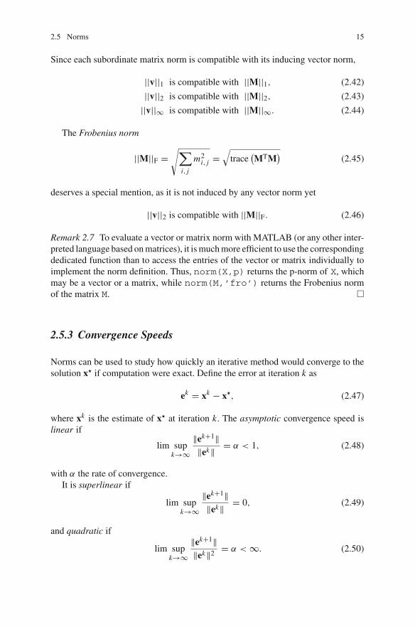
2.5.3 Convergence Speeds

Norms can be used to study how quickly an iterative method would converge to thesolution xν if computation were exact. Define the error at iteration k as

ek = xk − xν, (2.47)

where xk is the estimate of xν at iteration k. The asymptotic convergence speed islinear if

lim supk→∞

‖ek+1‖‖ek‖ = α < 1, (2.48)

with α the rate of convergence.It is superlinear if

lim supk→∞

‖ek+1‖‖ek‖ = 0, (2.49)

and quadratic if

lim supk→∞

‖ek+1‖‖ek‖2 = α < ∞. (2.50)

16 2 Notation and Norms

A method with quadratic convergence thus also has superlinear and linearconvergence. It is customary, however, to qualify a method with the best convergenceit achieves. Quadratic convergence is better that superlinear convergence, which isbetter than linear convergence.

Remember that these convergence speeds are asymptotic, valid when the errorhas become small enough, and that they do not take the effect of rounding intoaccount. They are meaningless if the initial vector x0 was too badly chosen for themethod to converge to xν. When the method does converge to xν, they may notdescribe accurately its initial behavior and will no longer be true when roundingerrors become predominant. They are nevertheless an interesting indication of whatcan be expected at best.

Reference

1. Vetter, W.: Derivative operations on matrices. IEEE Trans. Autom. Control 15, 241–244 (1970)

Chapter 3Solving Systems of Linear Equations

3.1 Introduction

Linear equations are first-order polynomial equations in their unknowns. A systemof linear equations can thus be written as

Ax = b, (3.1)

where the matrix A and the vector b are known and where x is a vector of unknowns.We assume in this chapter that

• all the entries of A, b and x are real numbers,• there are n scalar equations in n scalar unknowns (A is a square (n × n) matrix

and dim x = dim b = n),• these equations uniquely define x (A is invertible).

When A is invertible, the solution of (3.1) for x is unique, and given mathematicallyin closed form as x = A−1b. We are not interested here in this closed-form solution,and wish instead to compute x numerically from numerically known A and b. Thisproblem plays a central role in so many algorithms that it deserves a chapter ofits own. Systems of linear equations with more equations than unknowns will beconsidered in Sect. 9.2.

Remark 3.1 When A is square but singular (i.e., not invertible), its columns no longerform a basis of Rn , so the vector Ax cannot take all directions in R

n . The direction ofb will thus determine whether (3.1) admits infinitely many solutions for x or none.

When b can be expressed as a linear combination of columns of A, the equationsare linearly dependent and there is a continuum of solutions. The system x1 + x2 = 1and 2x1 + 2x2 = 2 corresponds to this situation.

When b cannot be expressed as a linear combination of columns of A, the equationsare incompatible and there is no solution. The system x1 + x2 = 1 and x1 + x2 = 2corresponds to this situation. �

É. Walter, Numerical Methods and Optimization, 17DOI: 10.1007/978-3-319-07671-3_3,© Springer International Publishing Switzerland 2014

18 3 Solving Systems of Linear Equations

Great books covering the topics of this chapter and Chap. 4 (as well as topicsrelevant to many others chapters) are [1–3].

3.2 Examples

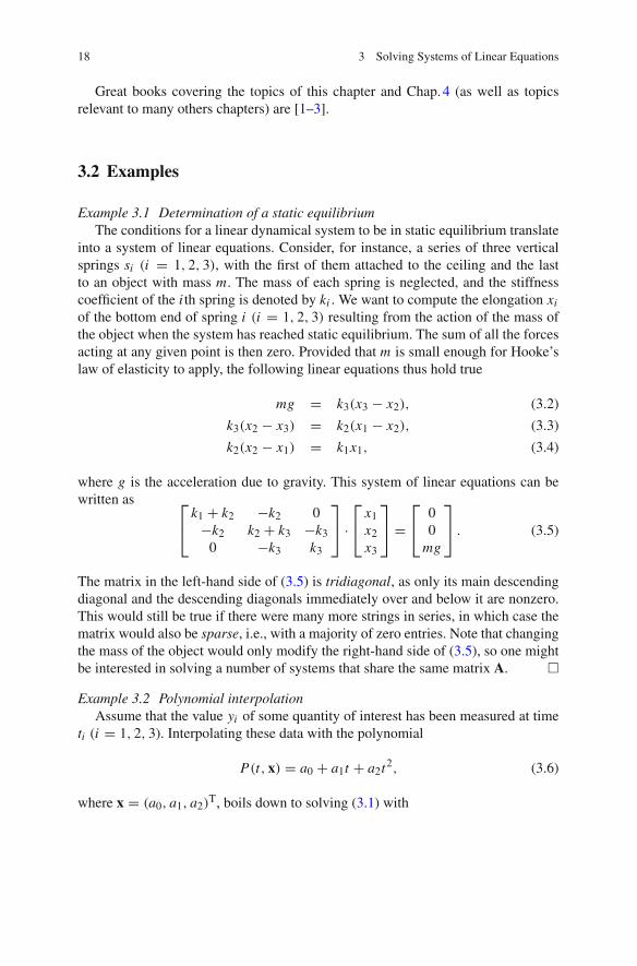
Example 3.1 Determination of a static equilibriumThe conditions for a linear dynamical system to be in static equilibrium translate

into a system of linear equations. Consider, for instance, a series of three verticalsprings si (i = 1, 2, 3), with the first of them attached to the ceiling and the lastto an object with mass m. The mass of each spring is neglected, and the stiffnesscoefficient of the i th spring is denoted by ki . We want to compute the elongation xi

of the bottom end of spring i (i = 1, 2, 3) resulting from the action of the mass ofthe object when the system has reached static equilibrium. The sum of all the forcesacting at any given point is then zero. Provided that m is small enough for Hooke’slaw of elasticity to apply, the following linear equations thus hold true

mg = k3(x3 − x2), (3.2)

k3(x2 − x3) = k2(x1 − x2), (3.3)

k2(x2 − x1) = k1x1, (3.4)

where g is the acceleration due to gravity. This system of linear equations can bewritten as

⎡k1 + k2 −k2 0

−k2 k2 + k3 −k30 −k3 k3

⎢

⎣ ·

⎡x1x2x3

⎢

⎣ =

⎡00

mg

⎢

⎣ . (3.5)

The matrix in the left-hand side of (3.5) is tridiagonal, as only its main descendingdiagonal and the descending diagonals immediately over and below it are nonzero.This would still be true if there were many more strings in series, in which case thematrix would also be sparse, i.e., with a majority of zero entries. Note that changingthe mass of the object would only modify the right-hand side of (3.5), so one mightbe interested in solving a number of systems that share the same matrix A. �

Example 3.2 Polynomial interpolationAssume that the value yi of some quantity of interest has been measured at time

ti (i = 1, 2, 3). Interpolating these data with the polynomial

P(t, x) = a0 + a1t + a2t2, (3.6)

where x = (a0, a1, a2)T, boils down to solving (3.1) with

3.2 Examples 19

A =

⎤⎡1 t1 t2

1

1 t2 t22

1 t3 t23

⎢

⎥⎣ and b =

⎡y1y2y3

⎢

⎣ . (3.7)

For more on interpolation, see Chap. 5. �

3.3 Condition Number(s)

The notion of condition number plays a central role in assessing the intrinsic difficultyof solving a given numerical problem independently of the algorithm to be employed[4, 5]. It can thus be used to detect problems about which one should be particularlycareful. We limit ourselves here to the problem of solving (3.1) for x. In general, A andb are imperfectly known, for at least two reasons. First, the mere fact of convertingreal numbers to their floating-point representation or of performing floating-pointcomputations almost always entails approximations. Moreover, the entries of A andb often result from imprecise measurements. It is thus important to quantify the effectthat perturbations on A and b may have on the solution x.

Substitute A + ∂A for A and b + ∂b for b, and define ⎦x as the solution of theperturbed system

(A + ∂A)⎦x = b + ∂b. (3.8)

The difference between the solutions of the perturbed system (3.8) and originalsystem (3.1) is

∂x =⎦x − x. (3.9)

It satisfies∂x = A−1 [∂b − (∂A)⎦x] . (3.10)

Provided that compatible norms are used, this implies that

||∂x|| � ||A−1|| · (||∂b|| + ||∂A|| · ||⎦x||) . (3.11)

Divide both sides of (3.11) by ||⎦x||, and multiply the right-hand side of the result by||A||/||A|| to get

||∂x||||⎦x|| � ||A−1|| · ||A||

⎞ ||∂b||||A|| · ||⎦x|| + ||∂A||

||A||⎠

. (3.12)

The multiplicative coefficient ||A−1|| · ||A|| appearing in the right-hand side of (3.12)is the condition number of A

cond A = ||A−1|| · ||A||. (3.13)

20 3 Solving Systems of Linear Equations

It quantifies the consequences of an error on A or b on the error on x. We wish it tobe as small as possible, so that the solution be as insensitive as possible to the errors∂A and ∂b.

Remark 3.2 When the errors on b are negligible, (3.12) becomes

||∂x||||⎦x|| � (cond A) ·

⎞ ||∂A||||A||

⎠. (3.14)

�

Remark 3.3 When the errors on A are negligible,

∂x = A−1∂b, (3.15)

so√∂x√ � √A−1√ · √∂b√. (3.16)

Now (3.1) implies that√b√ � √A√ · √x√, (3.17)

and (3.16) and (3.17) imply that

√∂x√ · √b√ � √A−1√ · √A√ · √∂b√ · √x√, (3.18)

so √∂x√√x√ � (cond A) ·

⎞ ||∂b||||b||

⎠. (3.19)

�

Since1 = ||I|| = ||A−1 · A|| � ||A−1|| · ||A||, (3.20)

the condition number of A satisfies

cond A � 1. (3.21)

Its value depends on the norm used. For the spectral norm,

||A||2 = σmax(A), (3.22)

where σmax(A) is the largest singular value of A. Since

||A−1||2 = σmax(A−1) = 1

σmin(A), (3.23)

3.3 Condition Number(s) 21

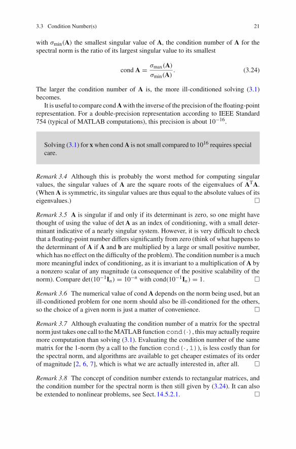
with σmin(A) the smallest singular value of A, the condition number of A for thespectral norm is the ratio of its largest singular value to its smallest

cond A = σmax(A)

σmin(A). (3.24)

The larger the condition number of A is, the more ill-conditioned solving (3.1)becomes.

It is useful to compare cond A with the inverse of the precision of the floating-pointrepresentation. For a double-precision representation according to IEEE Standard754 (typical of MATLAB computations), this precision is about 10−16.

Solving (3.1) for x when cond A is not small compared to 1016 requires specialcare.

Remark 3.4 Although this is probably the worst method for computing singularvalues, the singular values of A are the square roots of the eigenvalues of ATA.(When A is symmetric, its singular values are thus equal to the absolute values of itseigenvalues.) �

Remark 3.5 A is singular if and only if its determinant is zero, so one might havethought of using the value of det A as an index of conditioning, with a small deter-minant indicative of a nearly singular system. However, it is very difficult to checkthat a floating-point number differs significantly from zero (think of what happens tothe determinant of A if A and b are multiplied by a large or small positive number,which has no effect on the difficulty of the problem). The condition number is a muchmore meaningful index of conditioning, as it is invariant to a multiplication of A bya nonzero scalar of any magnitude (a consequence of the positive scalability of thenorm). Compare det(10−1In) = 10−n with cond(10−1In) = 1. �

Remark 3.6 The numerical value of cond A depends on the norm being used, but anill-conditioned problem for one norm should also be ill-conditioned for the others,so the choice of a given norm is just a matter of convenience. �

Remark 3.7 Although evaluating the condition number of a matrix for the spectralnorm just takes one call to the MATLAB function cond(·), this may actually requiremore computation than solving (3.1). Evaluating the condition number of the samematrix for the 1-norm (by a call to the function cond(·,1)), is less costly than forthe spectral norm, and algorithms are available to get cheaper estimates of its orderof magnitude [2, 6, 7], which is what we are actually interested in, after all. �

Remark 3.8 The concept of condition number extends to rectangular matrices, andthe condition number for the spectral norm is then still given by (3.24). It can alsobe extended to nonlinear problems, see Sect. 14.5.2.1. �

22 3 Solving Systems of Linear Equations

3.4 Approaches Best Avoided

For solving a system of linear equations numerically, matrix inversion shouldalmost always be avoided, as it requires useless computations.

Unless A has some specific structure that makes inversion particularly simple, oneshould thus think twice before inverting A to take advantage of the closed-formsolution

x = A−1b. (3.25)

Cramer’s rule for solving systems of linear equations, which requires the com-putation of ratios of determinants is the worst possible approach. Determinants arenotoriously difficult to compute accurately and computing these determinants isunnecessarily costly, even if much more economical methods than cofactor expan-sion are available.

3.5 Questions About A

A often has specific properties that may be taken advantage of and that may lead toselecting a specific method rather than systematically using some general-purposeworkhorse. It is thus important to address the following questions:

• Are A and b real (as assumed here)?• Is A square and invertible (as assumed here)?• Is A symmetric, i.e., such that AT = A?• Is A symmetric positive definite (denoted by A ∇ 0)? This means that A is sym-

metric and such that→v ⇒= 0, vTAv > 0, (3.26)

which implies that all of its eigenvalues are real and strictly positive.• If A is large, is it sparse, i.e., such that most of its entries are zeros?• Is A diagonally dominant, i.e., such that the absolute value of each of its diagonal

entries is strictly larger than the sum of the absolute values of all the other entriesin the same row?

• Is A tridiagonal, i.e., such that only its main descending diagonal and the diagonalsimmediately over and below are nonzero?

3.5 Questions About A 23

A =

⎤⎤⎤⎤⎤⎤⎤⎤⎤⎤⎤⎡

b1 c1 0 · · · · · · 0

a2 b2 c2 0...

0 a3. . .

. . .. . .

...

... 0. . .

. . .. . . 0

.... . .

. . . bn−1 cn−10 · · · · · · 0 an bn

⎢

⎥⎥⎥⎥⎥⎥⎥⎥⎥⎥⎥⎣

(3.27)

• Is A Toeplitz, i.e., such that all the entries on the same descending diagonal take the samevalue?

A =

⎤⎤⎤⎤⎤⎤⎡

h0 h−1 h−2 · · · h−n+1h1 h0 h−1 h−n+2...

. . .. . .

. . ....

.... . .

. . . h−1hn−1 hn−2 · · · h1 h0

⎢

⎥⎥⎥⎥⎥⎥⎣(3.28)

• Is A well-conditioned? (See Sect. 3.3.)

3.6 Direct Methods

Direct methods attempt to solve (3.1) for x in a finite number of steps. They requirea predictable amount of ressources and can be made quite robust, but scale poorlyon very large problems. This is in contrast with iterative methods, considered inSect. 3.7, which aim at generating a sequence of improving approximations of thesolution. Some iterative methods can deal with millions of unknowns, as encounteredfor instance when solving partial differential equations.

Remark 3.9 The distinction between direct and iterative method is not as clear cutas it may seem; results obtained by direct methods may be improved by iterativemethods (as in Sect. 3.6.4), and the most sophisticated iterative methods (presentedin Sect. 3.7.2) would find the exact solution in a finite number of steps if computationwere carried out exactly. �

3.6.1 Backward or Forward Substitution

Backward or forward substitution applies when A is triangular. This is less of a specialcase than it may seem, as several of the methods presented below and applicable togeneric linear systems involve solving triangular systems.

Backward substitution applies to the upper triangular system

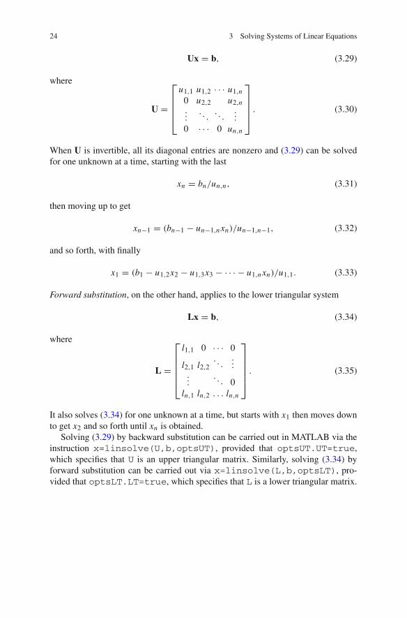
24 3 Solving Systems of Linear Equations

Ux = b, (3.29)

where

U =

⎤⎤⎤⎡

u1,1 u1,2 · · · u1,n

0 u2,2 u2,n...

. . .. . .

...

0 · · · 0 un,n

⎢

⎥⎥⎥⎣ . (3.30)

When U is invertible, all its diagonal entries are nonzero and (3.29) can be solvedfor one unknown at a time, starting with the last

xn = bn/un,n, (3.31)

then moving up to get

xn−1 = (bn−1 − un−1,n xn)/un−1,n−1, (3.32)

and so forth, with finally

x1 = (b1 − u1,2x2 − u1,3x3 − · · · − u1,n xn)/u1,1. (3.33)

Forward substitution, on the other hand, applies to the lower triangular system

Lx = b, (3.34)

where

L =

⎤⎤⎤⎤⎡

l1,1 0 · · · 0

l2,1 l2,2. . .

......

. . . 0ln,1 ln,2 . . . ln,n

⎢

⎥⎥⎥⎥⎣. (3.35)

It also solves (3.34) for one unknown at a time, but starts with x1 then moves downto get x2 and so forth until xn is obtained.

Solving (3.29) by backward substitution can be carried out in MATLAB via theinstruction x=linsolve(U,b,optsUT), provided that optsUT.UT=true,which specifies that U is an upper triangular matrix. Similarly, solving (3.34) byforward substitution can be carried out via x=linsolve(L,b,optsLT), pro-vided that optsLT.LT=true, which specifies that L is a lower triangular matrix.

3.6 Direct Methods 25

3.6.2 Gaussian Elimination

Gaussian elimination [8] transforms the original system (3.1) into an upper triangularsystem

Ux = v, (3.36)

by replacing each row of Ax and b by a suitable linear combination of such rows.This triangular system is then solved by backward substitution, one unknown at atime. All of this is carried out by the single MATLAB instruction x=A\b. Thisattractive one-liner actually hides the fact that A has been factored, and the resultingfactorization is thus not available for later use (for instance, to solve (3.1) with thesame A but another b).

When (3.1) must be solved for several right-hand sides bi (i = 1, . . . , m) allknown in advance, the system

Ax1 · · · xm = b1 · · · bm (3.37)

is similarly transformed by row combinations into

Ux1 · · · xm = v1 · · · vm . (3.38)

The solutions are then obtained by solving the triangular systems

Uxi = vi , i = 1, . . . , m. (3.39)

This classical approach for solving (3.1) has no advantage over LU factorizationpresented next. As it works simultaneously on A and b, Gaussian elimination for aright-hand side b not previously known cannot take advantage of past computationscarried out with other right-hand sides, even if A remains the same.

3.6.3 LU Factorization

LU factorization, a matrix reformulation of Gaussian elimination, is the basic work-horse to be used when A has no particular structure to be taken advantage of. Considerfirst its simplest version.

3.6.3.1 LU Factorization Without Pivoting

A is factored asA = LU, (3.40)

26 3 Solving Systems of Linear Equations

where L is lower triangular and U upper triangular. (It is also known asLR factorization, with L standing for left triangular and R for right triangular.)

When possible, this factorization is not unique, since L and U contain (n2 + n)

unknown entries whereas A has only n2 entries, which provide as many scalar rela-tions between L and U. It is therefore necessary to add n constraints to ensureuniqueness, so we set all the diagonal entries of L equal to one. Equation (3.40) thentranslates into

A =

⎤⎤⎤⎤⎤⎡

1 0 · · · 0

l2,1 1. . .

...

.... . .

. . . 0

ln,1 · · · ln,n−1 1

⎢

⎥⎥⎥⎥⎥⎣·

⎤⎤⎤⎤⎤⎡

u1,1 u1,2 · · · u1,n

0 u2,2 u2,n

.... . .

. . ....

0 · · · 0 un,n

⎢

⎥⎥⎥⎥⎥⎣. (3.41)

When (3.41) admits a solution for its unknowns li, j et ui, j , this solution can beobtained very simply by considering the equations in the proper order. Each unknownis then expressed as a function of entries of A and already computed entries of L andU. For the sake of notational simplicity, and because our purpose is not coding LUfactorization, we only illustrate this with a very small example.

Example 3.3 LU factorization without pivotingFor the system [

a1,1 a1,2a2,1 a2,2

]=

[1 0

l2,1 1

]·[

u1,1 u1,20 u2,2

], (3.42)

we get

u1,1 = a1,1, u1,2 = a1,2, l2,1u1,1 = a2,1 and l2,1u1,2 + u2,2 = a2,2. (3.43)

So, provided that a11 ⇒= 0,

l2,1 = a2,1

u1,1= a2,1

a1,1and u2,2 = a2,2 − l2,1u1,2 = a2,2 − a2,1

a1,1a1,2. (3.44)

�

Terms that appear in denominators, such as a1,1 in Example 3.3, are called pivots.LU factorization without pivoting fails whenever a pivot turns out to be zero.

After LU factorization, the system to be solved is

LUx = b. (3.45)

Its solution for x is obtained in two steps.First,

Ly = b (3.46)

3.6 Direct Methods 27

is solved for y. Since L is lower triangular, this is by forward substitution, eachequation providing the solution for a new unknown. As the diagonal entries of L areequal to one, this is particularly simple.

Second,Ux = y (3.47)

is solved for x. Since U is upper triangular, this is by backward substitution, eachequation again providing the solution for a new unknown.

Example 3.4 Failure of LU factorization without pivotingFor

A =[

0 11 0

],

the pivot a1,1 is equal to zero, so the algorithm fails unless pivoting is carried out, aspresented next. Note that it suffices here to permute the rows of A (as well as thoseof b) for the problem to disappear. �

Remark 3.10 When no pivot is zero but the magnitude of some of them is too small,pivoting plays a crucial role for improving the quality of LU factorization. �

3.6.3.2 Pivoting

Pivoting is a short name for reordering the equations (and possibly the variables) soas to avoid zero pivots. When only the equations are reordered, one speaks of partialpivoting, whereas total pivoting, not considered here, also involves reordering thevariables. (Total pivoting is seldom used, as it rarely provides better results thanpartial pivoting while being more expensive.)

Reordering the equations amounts to permuting the same rows in A and in b,which can be carried out by left-multiplying A and b by a suitable permutation matrix.The permutation matrix P that exchanges the i th and j th rows of A is obtained byexchanging the i th and j th rows of the identity matrix. Thus, for instance,

⎡0 0 11 0 00 1 0

⎢

⎣ ·

⎡b1b2b3

⎢

⎣ =

⎡b3b1b2

⎢

⎣ . (3.48)

Since det I = 1 and any exchange of two rows changes the sign of the determinant,we have

det P = ±1. (3.49)

P is an orthonormal matrix (also called unitary matrix), i.e., it is such that

PTP = I. (3.50)

28 3 Solving Systems of Linear Equations

The inverse of P is thus particularly easy to compute, as

P−1 = PT. (3.51)

Finally, the product of permutation matrices is a permutation matrix.

3.6.3.3 LU Factorization with Partial Pivoting

When computing the i th column of L, the rows i to n of A are reordered so asto ensure that the entry with the largest absolute value in the i th column gets onthe diagonal (if it is not already there). This guarantees that all the entries of L arebounded by one in absolute value. The resulting algorithm is described in [2].

Let P be the permutation matrix summarizing the requested row exchanges on Aand b. The system to be solved becomes

PAx = Pb, (3.52)

and LU factorization is carried out on PA, so

LUx = Pb. (3.53)

Solution for x is again in two steps. First,

Ly = Pb (3.54)

is solved for y, and thenUx = y (3.55)

is solved for x. Of course the (sparse) permutation matrix P need not be stored as an(n × n) matrix; it suffices to keep track of the corresponding row exchanges.

Remark 3.11 Algorithms solving systems of linear equations via LU factorizationwith partial or total pivoting are readily and freely available on the WEB with adetailed documentation (in LAPACK, for instance, see Chap. 15). The same remarkapplies to most of the methods presented in this book. In MATLAB, LU factorizationwith partial pivoting is achieved by the instruction [L,U,P]=lu(A). �

Remark 3.12 Although the pivoting strategy of LU factorization is not based onkeeping the condition number of the problem unchanged, the increase in this condi-tion number is mitigated, which makes LU with partial pivoting applicable even tosome very ill-conditioned problems. See Sect. 3.10.1 for an illustration. �

LU factorization is a first example of the decomposition approach to matrix com-putation [9], where a matrix is expressed as a product of factors. Other examplesare QR factorization (Sects. 3.6.5 and 9.2.3), SVD (Sects. 3.6.6 and 9.2.4), Cholesky

3.6 Direct Methods 29

factorization (Sect. 3.8.1), and Schur and spectral decompositions, both carried outby the QR algorithm (Sect. 4.3.6). By concentrating efforts on the development ofefficient, robust algorithms for a few important factorizations, numerical analystshave made it possible to produce highly effective packages for matrix computation,with surprisingly diverse applications. Huge savings can be achieved when a numberof problems share the same matrix, which then only needs to be factored once. OnceLU factorization has been carried out on a given matrix A, for instance, all the systems(3.1) that differ only by their vector b are easily solved with the same factorization,even if the values of b to be considered were not known when A was factored. Thisis a definite advantage over Gaussian elimination where the factorization of A ishidden in the solution of (3.1) for some pre-specified b.

3.6.4 Iterative Improvement

Let ⎦x be the numerical result obtained when solving (3.1) via LU factorization.The residual A⎦x − b should be small, but this does not guarantee that ⎦x is a goodapproximation of the mathematical solution x = A−1b. One may try to improve ⎦xby looking for the correction vector ∂x such that

A(⎦x + ∂x) = b, (3.56)

or equivalently thatA∂x = b − A⎦x. (3.57)

Remark 3.13 A is the same in (3.57) as in (3.1), so its LU factorization is alreadyavailable. �

Once ∂x has been obtained by solving (3.57), ⎦x is replaced by ⎦x + ∂x, and theprocedure may be iterated until convergence, with a stopping criterion on ||∂x||. It isadvisable to compute the residual b − A⎦x with extended precision, as it correspondsto the difference between hopefully similar floating-point quantities.

Spectacular improvements may be obtained for such a limited effort.

Remark 3.14 Iterative improvement is not limited to the solution of linear systemsof equations via LU factorization. �

3.6.5 QR Factorization

Any (n × n) invertible matrix A can be factored as

A = QR, (3.58)

30 3 Solving Systems of Linear Equations

where Q is an (n × n) orthonormal matrix, such that QTQ = In , and R is an (n × n)

invertible upper triangular matrix (which tradition persists in calling R instead ofU...). This QR factorization is unique if one imposes that the diagonal entries of Rare positive, which is not mandatory. It can be carried out in a finite number of steps.In MATLAB, this is achieved by the instruction [Q,R]=qr(A).

Multiply (3.1) on the left by QT while taking (3.58) into account, to get

Rx = QTb, (3.59)

which is easy to solve for x, as R is triangular.

For the spectral norm, the condition number of R is the same as that of A, since

ATA = (QR)T QR = RTQTQR = RTR. (3.60)

QR factorization therefore does not worsen conditioning. This is an advantageover LU factorization, which comes at the cost of more computation.

Remark 3.15 Contrary to LU factorization, QR factorization also applies to rectan-gular matrices, and will prove extremely useful in the solution of linear least-squaresproblems, see Sect. 9.2.3. �

At least in principle, Gram–Schmidt orthogonalization could be used to carry outQR factorization, but it suffers from numerical instability when the columns of A areclose to being linearly dependent. This is why the more robust approach presentedin the next section is usually preferred, although a modified Gram-Schmidt methodcould also be employed [10].

3.6.5.1 Householder Transformation

The basic tool for QR factorization is the Householder transformation, described bythe eponymous matrix

H(v) = I − 2vvT

vTv, (3.61)

where v is a vector to be chosen. The vector H(v)x is the symmetric of x with respectto the hyperplan passing through the origin O and orthogonal to v (Fig. 3.1).

The matrix H(v) is symmetric and orthonormal. Thus

H(v) = HT(v) and HT(v)H(v) = I, (3.62)

which implies thatH−1(v) = H(v). (3.63)

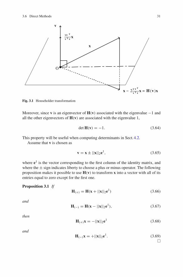
3.6 Direct Methods 31

x

O

v

vv T

v T vx

x − 2v v T

v T vx = H (v )x

Fig. 3.1 Householder transformation

Moreover, since v is an eigenvector of H(v) associated with the eigenvalue −1 andall the other eigenvectors of H(v) are associated with the eigenvalue 1,

det H(v) = −1. (3.64)

This property will be useful when computing determinants in Sect. 4.2.Assume that v is chosen as

v = x ± ||x||2e1, (3.65)

where e1 is the vector corresponding to the first column of the identity matrix, andwhere the ± sign indicates liberty to choose a plus or minus operator. The followingproposition makes it possible to use H(v) to transform x into a vector with all of itsentries equal to zero except for the first one.

Proposition 3.1 IfH(+) = H(x + ||x||2e1) (3.66)

andH(−) = H(x − ||x||2e1), (3.67)

thenH(+)x = −||x||2e1 (3.68)

andH(−)x = +||x||2e1. (3.69)

�

32 3 Solving Systems of Linear Equations

Proof If v = x ± ||x||2e1 then

vTv = xTx + √x√22(e

1)Te1 ± 2√x√2x1 = 2(√x√22 ± √x√2x1) = 2vTx. (3.70)

So

H(v)x = x − 2v⎞

vTxvTv

⎠= x − v = ∈||x||2e1. (3.71)

�

Among H(+) and H(−), one should choose

Hbest = H(x + sign (x1)||x||2e1), (3.72)

to protect oneself against the risk of having to compute the difference of floating-pointnumbers that are close to one another. In practice, the matrix H(v) is not formed.One computes instead the scalar

δ = 2vTxvTv

, (3.73)

and the vector

H(v)x = x − δv. (3.74)

3.6.5.2 Combining Householder Transformations

A is triangularized by submitting it to a series of Householder transformations, asfollows.

Start with A0 = A.Compute A1 = H1A0, where H1 is a Householder matrix that transforms the first

column of A0 into the first column of A1, all the entries of which are zeros exceptfor the first one. Based on Proposition 3.1, take

H1 = H(a1 + sign(a11)||a1||2e1), (3.75)

where a1 is the first column of A0.Iterate to get

Ak+1 = Hk+1Ak, k = 1, . . . , n − 2. (3.76)

Hk+1 is in charge of shaping the (k +1)-st column of Ak while leaving the k columnsto its left unchanged. Let ak+1 be the vector consisting of the last (n − k) entriesof the (k + 1)-st column of Ak . The Householder transformation must modify onlyak+1, so

3.6 Direct Methods 33

Hk+1 =[

Ik 00 H(ak+1 + sign(ak+1

1 )∥∥ak+1

∥∥2 e1)

]. (3.77)

In the next equation, for instance, the top and bottom entries of a3 are indicated bythe symbol ×:

A3 =

⎤⎤⎤⎤⎤⎤⎡

• • • · · · •0 • • · · · •... 0 × . . .

......

...... • •

0 0 × • •

⎢

⎥⎥⎥⎥⎥⎥⎣. (3.78)

In (3.77), e1 has the same dimension as ak+1 and all its entries are again zero, exceptfor the first one, which is equal to one.

At each iteration, the matrix H(+) or H(−) that leads to the more stable numericalcomputation is selected, see (3.72). Finally

R = Hn−1Hn−2 · · · H1A, (3.79)

or equivalently

A = (Hn−1Hn−2 · · · H1)−1R = H−1

1 H−12 · · · H−1

n−1R = QR. (3.80)

Take (3.63) into account to get

Q = H1H2 · · · Hn−1. (3.81)

Instead of using Householder transformations, one may implement QR factoriza-tion via Givens rotations [2], which are also robust, orthonormal transformations,but this makes computation more complex without improving performance.

3.6.6 Singular Value Decomposition

Singular value decomposition (SVD) [11] has turned out to be one of the most fruitfulideas in the theory of matrices [12]. Although it is mainly used on rectangular matrices(see Sect. 9.2.4, where the procedure is explained in more detail), it can also be appliedto any square matrix A, which it transforms into a product of three square matrices

A = U�VT. (3.82)

U and V are orthonormal, i.e.,

34 3 Solving Systems of Linear Equations

UTU = VTV = I, (3.83)

which makes their inversion particularly easy, as

U−1 = UT and V−1 = VT. (3.84)

� is a diagonal matrix, with diagonal entries equal to the singular values of A, socond A for the spectral norm is trivial to evaluate from the SVD. In this chapter, A isassumed to be invertible, which implies that no singular value is zero and � is invert-ible. In MATLAB, the SVD of A is achieved by the instruction [U,S,V]=svd(A).

Equation (3.1) translates into

U�VTx = b, (3.85)

sox = V�−1UTb, (3.86)

with �−1 trivial to evaluate as � is diagonal. As SVD is significantly more complexthan QR factorization, one may prefer the latter.

When cond A is too large, solving (3.1) becomes impossible using floating-pointnumbers, even via QR factorization. A better approximate solution may then beobtained by replacing (3.86) by

⎦x = V⎦�−1UTb, (3.87)

where ⎦�−1is a diagonal matrix such that

⎦�−1i,i =

{1/σi,i if σi,i > ∂

0 otherwise, (3.88)

with ∂ a positive threshold to be chosen by the user. This amounts to replacingany singular value of A that is smaller than ∂ by zero, thus pretending that (3.1)has infinitely many solutions, and then picking up the solution with the smallestEuclidean norm. See Sect. 9.2.6 for more details on this regularization approach inthe context of least squares. This approach should be used with a lot of caution here,however, as the quality of the approximate solution ⎦x provided by (3.87) dependsheavily on the value taken by b. Assume, for instance, that A is symmetric positivedefinite, and that b is an eigenvector of A associated with some very small eigenvalueαb, such that √b√2 = 1. The mathematical solution of (3.1)

x = 1

αbb (3.89)

then has a very large Euclidean norm, and should thus be completely different from⎦x, as the eigenvalue αb is also a (very small) singular value of A and 1/αb will be

3.6 Direct Methods 35

replaced by zero in the computation of⎦x. Examples of ill-posed problems for whichregularization via SVD gives interesting results are in [13].

3.7 Iterative Methods

In very large-scale problems such as those involved in the solution of partial dif-ferential equations, A is typically sparse, which should be taken advantage of. Thedirect methods in Sect. 3.6 become difficult to use, because sparsity is usually lostduring the factorization of A. One may then use sparse direct solvers (not presentedhere), which permute equations and unknowns in an attempt to minimize fill-in inthe factors. This is a complex optimization problem in itself, so iterative methods arean attractive alternative [2, 14].

3.7.1 Classical Iterative Methods

These methods are slow and now seldom used, but simple to understand. They serveas an introduction to the more modern Krylov subspace iteration of Sect. 3.7.2.

3.7.1.1 Principle

To solve (3.1) for x, decompose A into a sum of two matrices

A = A1 + A2, (3.90)

with A1 (easily) invertible, so as to ensure

x = −A−11 A2x + A−1

1 b. (3.91)

Define M = −A−11 A2 and v = A−1

1 b to get

x = Mx + v. (3.92)

The idea is to choose the decomposition (3.90) in such a way that the recursion

xk+1 = Mxk + v (3.93)

converges to the solution of (3.1) when k tends to infinity. This will be the case ifand only if all the eigenvalues of M are strictly inside the unit circle.

36 3 Solving Systems of Linear Equations

The methods considered below differ in how A is decomposed. We assume thatall diagonal entries of A are nonzero, and write

A = D + L + U, (3.94)

where D is a diagonal invertible matrix with the same diagonal entries as A, L isa lower triangular matrix with zero main descending diagonal, and U is an uppertriangular matrix also with zero main descending diagonal.

3.7.1.2 Jacobi Iteration

In the Jacobi iteration, A1 = D and A2 = L + U, so

M = −D−1(L + U) and v = D−1b. (3.95)

The scalar interpretation of this method is as follows. The j th row of (3.1) is

n∑

i=1

a j,i xi = b j . (3.96)

Since a j, j ⇒= 0 by hypothesis, it can be rewritten as

x j = b j − ∑i ⇒= j a j,i xi

a j, j, (3.97)

which expresses x j as a function of the other unknowns. A Jacobi iteration computes

xk+1j = b j − ∑

i ⇒= j a j,i xki

a j, j, j = 1, . . . , n. (3.98)

A sufficient condition for convergence to the solution xρ of (3.1) (whatever the initialvector x0) is that A be diagonally dominant. This condition is not necessary, andconvergence may take place under less restrictive conditions.

3.7.1.3 Gauss–Seidel Iteration

In the Gauss–Seidel iteration, A1 = D + L and A2 = U, so

M = −(D + L)−1U and v = (D + L)−1b. (3.99)

The scalar interpretation becomes

3.7 Iterative Methods 37

xk+1j = b j − ∑ j−1

i=1 a j,i xk+1i − ∑n

i= j+1 a j,i xki

a j, j, j = 1, . . . , n. (3.100)

Note the presence of xk+1i on the right-hand side of (3.100). The components of xk+1

that have already been evaluated are thus used in the computation of those that havenot. This speeds up convergence and makes it possible to save memory space.

Remark 3.16 The behavior of the Gauss–Seidel method depends on how the vari-ables are ordered in x, contrary to what happens with the Jacobi method. �

As with the Jacobi method, a sufficient condition for convergence to the solutionxρ of (3.1) (whatever the initial vector x0) is that A be diagonally dominant. Thiscondition is again not necessary, and convergence may take place under less restrictiveconditions.

3.7.1.4 Successive Over-Relaxation

The successive over-relaxation method (SOR) was developed in the context of solvingpartial differential equations [15]. It rewrites (3.1) as

(D + σL)x = σb − [σU + (σ − 1)D]x, (3.101)

where σ ⇒= 0 is the relaxation factor, and iterates solving

(D + σL)xk+1 = σb − [σU + (σ − 1)D]xk (3.102)

for xk+1. As D + σL is lower triangular, this is done by forward substitution, andequivalent to writing

xk+1j = (1 − σ)xk

j + σb j − ∑ j−1

i=1 a j,i xk+1i − ∑n

i= j+1 a j,i xki

a j, j, j = 1, . . . , n.

(3.103)As a result,

xk+1 = (1 − σ)xk + σxk+1GS , (3.104)

where xk+1GS is the approximation of the solution xρ suggested by the Gauss–Seidel

iteration.A necessary condition for convergence is σ ∈ [0, 2]. For σ = 1, the Gauss–

Seidel method is recovered. When σ < 1 the method is under-relaxed, whereas it isover-relaxed if σ > 1. The optimal value of σ depends on A, but over-relaxation isusually preferred, where the displacements suggested by the Gauss–Seidel methodare increased. The convergence of the Gauss–Seidel method may thus be acceleratedby extrapolating on iteration results. Methods are available to adapt σ based on past

38 3 Solving Systems of Linear Equations

behavior. They have largely lost their interest with the advent of Krylov subspaceiteration, however.

3.7.2 Krylov Subspace Iteration

Krylov subspace iteration [16, 17] has superseded classical iterative approaches,which may turn out to be very slow or even fail to converge. It was dubbed in [18]one of the ten algorithms with the greatest influence on the development and practiceof science and engineering in the twentieth century.

3.7.2.1 From Jacobi to Krylov

Jacobi iteration hasxk+1 = −D−1(L + U)xk + D−1b. (3.105)

Equation (3.94) implies that L + U = A − D, so

xk+1 = (I − D−1A)xk + D−1b. (3.106)

Since the true solution xρ = A−1b is unknown, the error

∂xk = xk − xρ (3.107)

cannot be computed, and the residual

rk = b − Axk = −A(xk − xρ) = −A∂xk (3.108)

is used instead to characterize the quality of the approximate solution obtained sofar. Normalize the system of equations to be solved to ensure that D = I. Then

xk+1 = (I − A)xk + b

= xk + rk . (3.109)

Subtract xρ from both sides of (3.109), and left multiply the result by −A to get

rk+1 = rk − Ark . (3.110)

The recursion (3.110) implies that

rk ∈ span{r0, Ar0, . . . , Akr0}, (3.111)

3.7 Iterative Methods 39

and (3.109) then implies that

xk − x0 =k−1∑

i=0

ri . (3.112)

Therefore,xk ∈ x0 + span{r0, Ar0, . . . , Ak−1r0}, (3.113)

where span{r0, Ar0, . . . , Ak−1r0} is the kth Krylov subspace generated by A fromr0, denoted by Kk(A, r0).

Remark 3.17 The definition of Krylov subspaces implies that

Kk−1(A, r0) ⊂ Kk(A, r0), (3.114)

and that each iteration increases the dimension of search space at most by one.Assume, for instance, that x0 = 0, which implies that r0 = b, and that b is aneigenvector of A such that

Ab = αb. (3.115)

Then→k � 1, span{r0, Ar0, . . . , Ak−1r0} = span{b}, (3.116)

This is appropriate, as the solution is x = α−1b. �

Remark 3.18 Let Pn(α) be the characteristic polynomial of A,

Pn(α) = det(A − αIn). (3.117)

The Cayley-Hamilton theorem states that Pn(A) is the zero (n × n) matrix. In otherwords, An is a linear combination of An−1, An−2, . . . , In , so

→k � n, Kk(A, r0) = Kn(A, r0), (3.118)

and the dimension of the space in which search takes place does not increase afterthe first n iterations. �

A crucial point, not proved here, is that there exists ν � n such that

xρ ∈ x0 + Kν(A, r0). (3.119)

In principle, one may thus hope to get the solution in no more than n = dim xiterations in Krylov subspaces, whereas for Jacobi, Gauss–Seidel or SOR iterationsno such bound is available. In practice, with floating-point computations, one maystill get better results by iterating until the solution is deemed satisfactory.

40 3 Solving Systems of Linear Equations

3.7.2.2 A Is Symmetric Positive Definite

When A ∇ 0, conjugate-gradient methods [19–21] are the iterative approach ofchoice to this day. The approximate solution is sought for by minimizing

J (x) = 1

2xTAx − bTx. (3.120)

Using theoretical optimality conditions presented in Sect. 9.1, it is easy to show thatthe unique minimizer of this cost function is indeed ⎦x = A−1b. Starting from xk ,the approximation of xρ at iteration k, xk+1 is computed by line search along somedirection dk as

xk+1(αk) = xk + αkdk . (3.121)

It is again easy to show that J (xk+1(αk)) is minimum if

αk = (dk)T(b − Axk)

(dk)TAdk. (3.122)

The search direction dk is taken so as to ensure that

(di )TAdk = 0, i = 0, . . . , k − 1, (3.123)

which means that it is conjugate with respect to A (or A-orthogonal) with all theprevious search directions. With exact computation, this would ensure convergenceto⎦x in at most n iterations. Because of the effect of rounding errors, it may be usefulto allow more than n iterations, although n may be so large that n iterations is actuallymore than can be achieved. (One often gets a useful approximation of the solutionin less than n iterations.)

After n iterations,

xn = x0 +n−1∑

i=0

αi di , (3.124)

soxn ∈ x0 + span{d0, . . . , dn−1}. (3.125)

A Krylov-space solver is obtained if the search directions are such that

span{d0, . . . , di } = Ki+1(A, r0), i = 0, 1, . . . (3.126)

This can be achieved with an amazingly simple algorithm [19, 21], summarized inTable 3.1. See also Sect. 9.3.4.6 and Example 9.8.

Remark 3.19 The notation := in Table 3.1 means that the variable on the left-handsign is assigned the value resulting of the evaluation of the expression on the

3.7 Iterative Methods 41

Table 3.1 Krylov-spacesolver

r0 := b − Ax0,

d0 := r0,

∂0 := √r0√22,

k := 0.

While ||rk ||2 > tol, compute∂∞

k := (dk)TAdk ,

αk := ∂k/∂∞k ,

xk+1 := xk + αkdk ,

rk+1 := rk − αkAdk ,

∂k+1 := √rk+1√22,

βk := ∂k+1/∂k ,

dk+1 := rk+1 + βkdk ,

k := k + 1.

right-hand side. It should not be confused with the equal sign, and one may writek := k + 1 whereas k = k + 1 would make no sense. In MATLAB and a number ofother programming languages, however, the sign = is used instead of :=. �

3.7.2.3 A Is Not Symmetric Positive Definite

This is a much more complicated and costly situation. Specific methods, not detailedhere, have been developed for symmetric matrices that are not positive definite [22],as well as for nonsymmetric matrices [23, 24].

3.7.2.4 Preconditioning

The convergence speed of Krylov iteration strongly depends on the condition numberof A. Spectacular acceleration may be achieved by replacing (3.1) by

MAx = Mb, (3.127)

where M is a suitably chosen preconditioning matrix, and a considerable amount ofresearch has been devoted to this topic [25, 26]. As a result, modern preconditionedKrylov methods converge must faster and for a much wider class of matrices thanthe classical iterative methods of Sect. 3.7.1.

One possible approach for choosing M is to look for a sparse approximation ofthe inverse of A by solving

⎦M = arg minM∈S

√In − AM√F, (3.128)

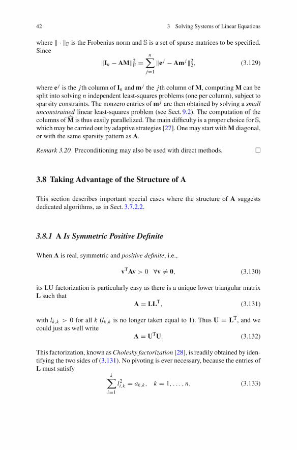
42 3 Solving Systems of Linear Equations

where √ · √F is the Frobenius norm and S is a set of sparse matrices to be specified.Since

√In − AM√2F =

n∑

j=1

√e j − Am j√22, (3.129)

where e j is the j th column of In and m j the j th column of M, computing M can besplit into solving n independent least-squares problems (one per column), subject tosparsity constraints. The nonzero entries of m j are then obtained by solving a smallunconstrained linear least-squares problem (see Sect. 9.2). The computation of thecolumns of ⎦M is thus easily parallelized. The main difficulty is a proper choice for S,which may be carried out by adaptive strategies [27]. One may start with M diagonal,or with the same sparsity pattern as A.

Remark 3.20 Preconditioning may also be used with direct methods. �

3.8 Taking Advantage of the Structure of A

This section describes important special cases where the structure of A suggestsdedicated algorithms, as in Sect. 3.7.2.2.

3.8.1 A Is Symmetric Positive Definite

When A is real, symmetric and positive definite, i.e.,

vTAv > 0 →v ⇒= 0, (3.130)

its LU factorization is particularly easy as there is a unique lower triangular matrixL such that

A = LLT, (3.131)

with lk,k > 0 for all k (lk,k is no longer taken equal to 1). Thus U = LT, and wecould just as well write

A = UTU. (3.132)

This factorization, known as Cholesky factorization [28], is readily obtained by iden-tifying the two sides of (3.131). No pivoting is ever necessary, because the entries ofL must satisfy

k∑

i=1

l2i,k = ak,k, k = 1, . . . , n, (3.133)

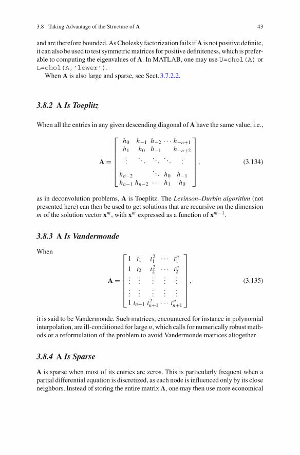
3.8 Taking Advantage of the Structure of A 43

and are therefore bounded. As Cholesky factorization fails if A is not positive definite,it can also be used to test symmetric matrices for positive definiteness, which is prefer-able to computing the eigenvalues of A. In MATLAB, one may use U=chol(A) orL=chol(A,’lower’).

When A is also large and sparse, see Sect. 3.7.2.2.

3.8.2 A Is Toeplitz

When all the entries in any given descending diagonal of A have the same value, i.e.,

A =

⎤⎤⎤⎤⎤⎤⎡

h0 h−1 h−2 · · · h−n+1h1 h0 h−1 h−n+2...

. . .. . .

. . ....

hn−2. . . h0 h−1

hn−1 hn−2 · · · h1 h0

⎢

⎥⎥⎥⎥⎥⎥⎣, (3.134)

as in deconvolution problems, A is Toeplitz. The Levinson–Durbin algorithm (notpresented here) can then be used to get solutions that are recursive on the dimensionm of the solution vector xm , with xm expressed as a function of xm−1.

3.8.3 A Is Vandermonde

When

A =

⎤⎤⎤⎤⎤⎤⎤⎡

1 t1 t21 · · · tn

1

1 t2 t22 · · · tn

2...

......

......

......

......

...

1 tn+1 t2n+1 · · · tn

n+1

⎢

⎥⎥⎥⎥⎥⎥⎥⎣

, (3.135)

it is said to be Vandermonde. Such matrices, encountered for instance in polynomialinterpolation, are ill-conditioned for large n, which calls for numerically robust meth-ods or a reformulation of the problem to avoid Vandermonde matrices altogether.

3.8.4 A Is Sparse

A is sparse when most of its entries are zeros. This is particularly frequent when apartial differential equation is discretized, as each node is influenced only by its closeneighbors. Instead of storing the entire matrix A, one may then use more economical

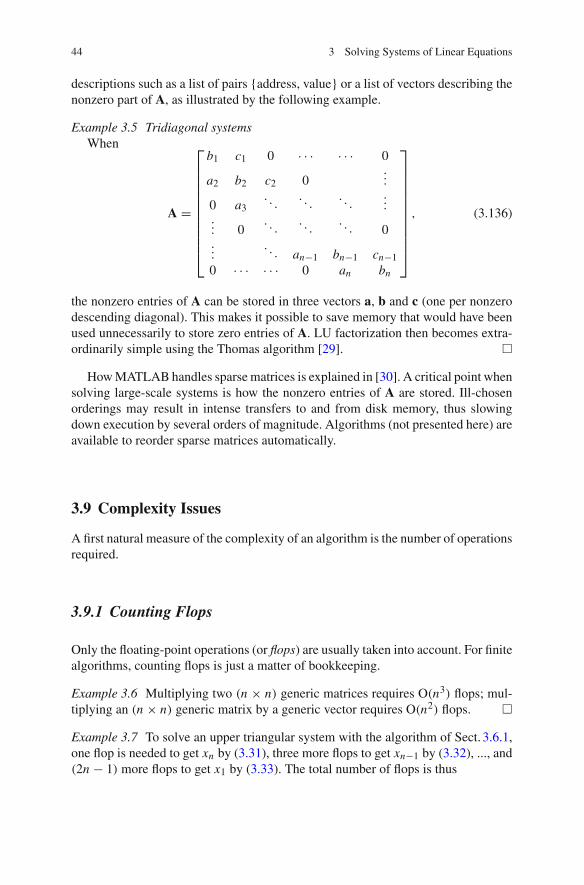
44 3 Solving Systems of Linear Equations

descriptions such as a list of pairs {address, value} or a list of vectors describing thenonzero part of A, as illustrated by the following example.

Example 3.5 Tridiagonal systemsWhen

A =

⎤⎤⎤⎤⎤⎤⎤⎤⎤⎤⎡

b1 c1 0 · · · · · · 0

a2 b2 c2 0...

0 a3. . .

. . .. . .

...... 0

. . .. . .

. . . 0...

. . . an−1 bn−1 cn−10 · · · · · · 0 an bn

⎢

⎥⎥⎥⎥⎥⎥⎥⎥⎥⎥⎣

, (3.136)

the nonzero entries of A can be stored in three vectors a, b and c (one per nonzerodescending diagonal). This makes it possible to save memory that would have beenused unnecessarily to store zero entries of A. LU factorization then becomes extra-ordinarily simple using the Thomas algorithm [29]. �

How MATLAB handles sparse matrices is explained in [30]. A critical point whensolving large-scale systems is how the nonzero entries of A are stored. Ill-chosenorderings may result in intense transfers to and from disk memory, thus slowingdown execution by several orders of magnitude. Algorithms (not presented here) areavailable to reorder sparse matrices automatically.

3.9 Complexity Issues

A first natural measure of the complexity of an algorithm is the number of operationsrequired.

3.9.1 Counting Flops

Only the floating-point operations (or flops) are usually taken into account. For finitealgorithms, counting flops is just a matter of bookkeeping.

Example 3.6 Multiplying two (n × n) generic matrices requires O(n3) flops; mul-tiplying an (n × n) generic matrix by a generic vector requires O(n2) flops. �

Example 3.7 To solve an upper triangular system with the algorithm of Sect. 3.6.1,one flop is needed to get xn by (3.31), three more flops to get xn−1 by (3.32), ..., and(2n − 1) more flops to get x1 by (3.33). The total number of flops is thus

3.9 Complexity Issues 45

1 + 3 + · · · + (2n − 1) = n2. (3.137)

�

Example 3.8 When A is tridiagonal, solving (3.1) with the Thomas algorithm(a specialization of LU factorization) can be done in (8n − 6) flops only [29]. �

For a generic (n × n) matrix A, the number of flops required to solve a linearsystem of equations turns out to be much higher than in Examples 3.7 and 3.8:

• LU factorization requires (2n3/3) flops. Solving each of the two resulting triangu-lar systems to get the solution for one right-hand side requires about n2 more flops,so the total number of flops for m right-hand sides is about

[(2n3/3) + m(2n2)

].

• QR factorization requires 2n3 flops, and the total number of flops for m right-handsides is 2n3 + 3mn2.

• A particularly efficient implementation of SVD [2] requires[(20n3/3) + O(n2)

]

flops.

Remark 3.21 For a generic (n × n) matrix A, LU, QR and SVD factorizations thusall require O(n3) flops. They can nevertheless be ranked, from the point of view ofthe number of flops required, as

LU < QR < SVD.

For small problems, each of these factorizations is obtained very quickly anyway, sothese issues become relevant only for large-scale problems or for problems that haveto be solved many times in an iterative algorithm. �

When A is symmetric positive definite, Cholesky factorization applies, whichrequires only n3/3 flops. The total number of flops for m right-hand sides thusbecomes

[(n3/3) + m(2n2)

].

The number of flops required by iterative methods depends on the degree ofsparsity of A, on the convergence speed of these methods (which itself depends onthe problem considered) and on the degree of approximation one is willing to toleratein the solution. For Krylov-space solvers, dim x is an upper bound of the numberiterations needed to get an exact solution in the absence of rounding errors. This isa considerable advantage over classical iterative methods.

3.9.2 Getting the Job Done Quickly

When dealing with a large-scale linear system, as often encountered in real-life appli-cations, the number of flops is just one ingredient in the determination of the timeneeded to get the solution, because it may take more time to move the relevant data inand out of the arithmetic unit(s) than to perform the flops. It is important to realize that

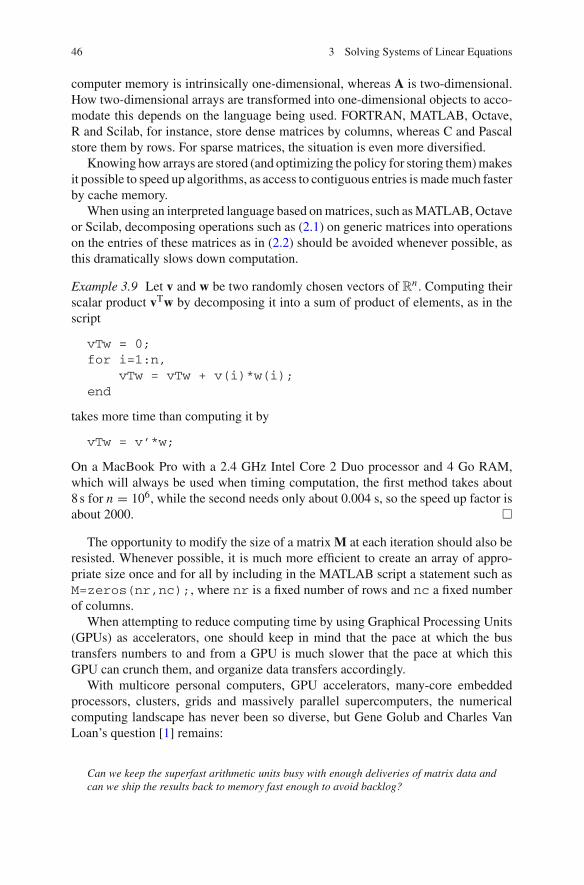
46 3 Solving Systems of Linear Equations

computer memory is intrinsically one-dimensional, whereas A is two-dimensional.How two-dimensional arrays are transformed into one-dimensional objects to acco-modate this depends on the language being used. FORTRAN, MATLAB, Octave,R and Scilab, for instance, store dense matrices by columns, whereas C and Pascalstore them by rows. For sparse matrices, the situation is even more diversified.

Knowing how arrays are stored (and optimizing the policy for storing them) makesit possible to speed up algorithms, as access to contiguous entries is made much fasterby cache memory.

When using an interpreted language based on matrices, such as MATLAB, Octaveor Scilab, decomposing operations such as (2.1) on generic matrices into operationson the entries of these matrices as in (2.2) should be avoided whenever possible, asthis dramatically slows down computation.

Example 3.9 Let v and w be two randomly chosen vectors of Rn . Computing theirscalar product vTw by decomposing it into a sum of product of elements, as in thescript

vTw = 0;for i=1:n,

vTw = vTw + v(i)*w(i);end

takes more time than computing it by

vTw = v’*w;

On a MacBook Pro with a 2.4 GHz Intel Core 2 Duo processor and 4 Go RAM,which will always be used when timing computation, the first method takes about8 s for n = 106, while the second needs only about 0.004 s, so the speed up factor isabout 2000. �

The opportunity to modify the size of a matrix M at each iteration should also beresisted. Whenever possible, it is much more efficient to create an array of appro-priate size once and for all by including in the MATLAB script a statement such asM=zeros(nr,nc);, where nr is a fixed number of rows and nc a fixed numberof columns.

When attempting to reduce computing time by using Graphical Processing Units(GPUs) as accelerators, one should keep in mind that the pace at which the bustransfers numbers to and from a GPU is much slower that the pace at which thisGPU can crunch them, and organize data transfers accordingly.

With multicore personal computers, GPU accelerators, many-core embeddedprocessors, clusters, grids and massively parallel supercomputers, the numericalcomputing landscape has never been so diverse, but Gene Golub and Charles VanLoan’s question [1] remains:

Can we keep the superfast arithmetic units busy with enough deliveries of matrix data andcan we ship the results back to memory fast enough to avoid backlog?

3.10 MATLAB Examples 47

3.10 MATLAB Examples

By means of short scripts and their results, this section demonstrates how easy itis to experiment with some of the methods described. Sections with the same titleand aim will follow in most chapters. They cannot serve as a substitute for a goodtutorial on MATLAB, of which there are many. The names given to the variables arehopefully self-explanatory. For instance, the variable A corresponds to the matrix A.

3.10.1 A Is Dense

MATLAB offers a number of options for solving (3.1). The simplest of them is touse Gaussian elimination

xGE = A\b;

No factorization of A is then available for later use, for instance for solving (3.1)with the same A and another b.

It may make more sense to choose a factorization and use it. For an LU factoriza-tion with partial pivoting, one may write

[L,U,P] = lu(A);% Same row exchange in b as in APb = P*b;

% Solve Ly = Pb, with L lower triangularopts_LT.LT = true;y = linsolve(L,Pb,opts_LT);

% Solve Ux = y, with U upper triangularopts_UT.UT = true;xLUP = linsolve(U,y,opts_UT);

which gives access to the factorization of A that has been carried out. A one-linerversion with the same result would be

xLUP = linsolve(A,b);

but L, U and P would then no longer be made available for further use.For a QR factorization, one may write

[Q,R] = qr(A);QTb = Q’*b;opts_UT.UT = true;x_QR = linsolve(R,QTb,opts_UT);

and for an SVD factorization

48 3 Solving Systems of Linear Equations

[U,S,V] = svd(A);xSVD = V*inv(S)*U’*b;

For an iterative solution via the Krylov method, one may use the function gmres,which does not require A to be positive definite [23], and write

xKRY = gmres(A,b);

Although the Krylov method is particularly interesting when A is large and sparse,nothing forbids using it on a small dense matrix, as here.

These five methods are used to solve (3.1) with

A =

⎤⎡1 2 3

4 5 6

7 8 9 + κ

⎢

⎥⎣ (3.138)

and

b =

⎡101112

⎢

⎣ , (3.139)

which translates into

A = [1, 2, 34, 5, 67, 8, 9 + alpha];

b = [10; 11; 12];

A is then singular for κ = 0, and its conditioning improves when κ increases. Forany κ > 0, it is easy to check that the exact solution is unique and given by

x =

⎡−28/329/3

0

⎢

⎣ ≈

⎡−9.33333333333333339.6666666666666667

0

⎢

⎣ . (3.140)

The fact that x3 = 0 explains why x is independent of the numerical value taken byκ. However, the difficulty of computing x accurately does depend on this value. Inall the results to be presented in the remainder of this chapter, the condition numberreferred to is for the spectral norm.

For κ = 10−13, cond A ≈ 1015 and

xGE =-9.297539149888147e+009.595078299776288e+003.579418344519016e-02

xLUP =-9.297539149888147e+00

3.10 MATLAB Examples 49

9.595078299776288e+003.579418344519016e-02

xQR =-9.553113553113528e+001.010622710622708e+01-2.197802197802198e-01

xSVD =-9.625000000000000e+001.025000000000000e+01-3.125000000000000e-01

gmres converged at iteration 2 to a solution withrelative residual 9.9e-15.xKRY =

-4.555555555555692e+001.111111111110619e-014.777777777777883e+00

LU factorization with partial pivoting turns out to have done a better job than QRfactorization or SVD on this ill-conditioned problem, for less computation. Thecondition numbers of the matrices involved are evaluated as follows

CondA = 1.033684444145846e+15

% LU factorizationCondL = 2.055595570492287e+00CondU = 6.920247514139799e+14

% QR factorization with partial pivotingCondP = 1CondQ = 1.000000000000000e+00CondR = 1.021209931367105e+15

% SVDCondU = 1.000000000000001e+00CondS = 1.033684444145846e+15CondV = 1.000000000000000e+00

For κ = 10−5, cond A ≈ 107 and

xGE =-9.333333332978063e+009.666666665956125e+003.552713679092771e-10

50 3 Solving Systems of Linear Equations

xLUP =-9.333333332978063e+009.666666665956125e+003.552713679092771e-10

xQR =-9.333333335508891e+009.666666671017813e+00-2.175583929062594e-09

xSVD =-9.333333335118368e+009.666666669771075e+00-1.396983861923218e-09

gmres converged at iteration 3 to a solutionwith relative residual 0.xKRY =

-9.333333333420251e+009.666666666840491e+00-8.690781427844740e-11

The condition numbers of the matrices involved are

CondA = 1.010884565427633e+07

% LU factorizationCondL = 2.055595570492287e+00CondU = 6.868613692978372e+06

% QR factorization with partial pivotingCondP = 1CondQ = 1.000000000000000e+00CondR = 1.010884565403081e+07

% SVDCondU = 1.000000000000000e+00CondS = 1.010884565427633e+07CondV = 1.000000000000000e+00

For κ = 1, cond A ≈ 88 and

xGE =-9.333333333333330e+009.666666666666661e+003.552713678800503e-15

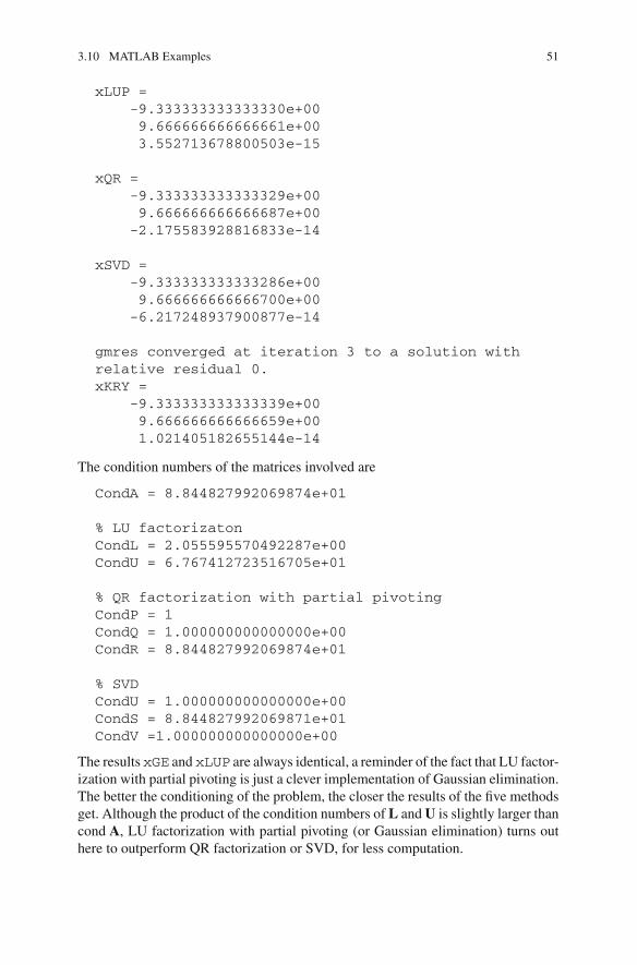
3.10 MATLAB Examples 51

xLUP =-9.333333333333330e+009.666666666666661e+003.552713678800503e-15

xQR =-9.333333333333329e+009.666666666666687e+00-2.175583928816833e-14

xSVD =-9.333333333333286e+009.666666666666700e+00-6.217248937900877e-14

gmres converged at iteration 3 to a solution withrelative residual 0.xKRY =

-9.333333333333339e+009.666666666666659e+001.021405182655144e-14

The condition numbers of the matrices involved are

CondA = 8.844827992069874e+01

% LU factorizatonCondL = 2.055595570492287e+00CondU = 6.767412723516705e+01

% QR factorization with partial pivotingCondP = 1CondQ = 1.000000000000000e+00CondR = 8.844827992069874e+01

% SVDCondU = 1.000000000000000e+00CondS = 8.844827992069871e+01CondV =1.000000000000000e+00

The results xGE and xLUP are always identical, a reminder of the fact that LU factor-ization with partial pivoting is just a clever implementation of Gaussian elimination.The better the conditioning of the problem, the closer the results of the five methodsget. Although the product of the condition numbers of L and U is slightly larger thancond A, LU factorization with partial pivoting (or Gaussian elimination) turns outhere to outperform QR factorization or SVD, for less computation.

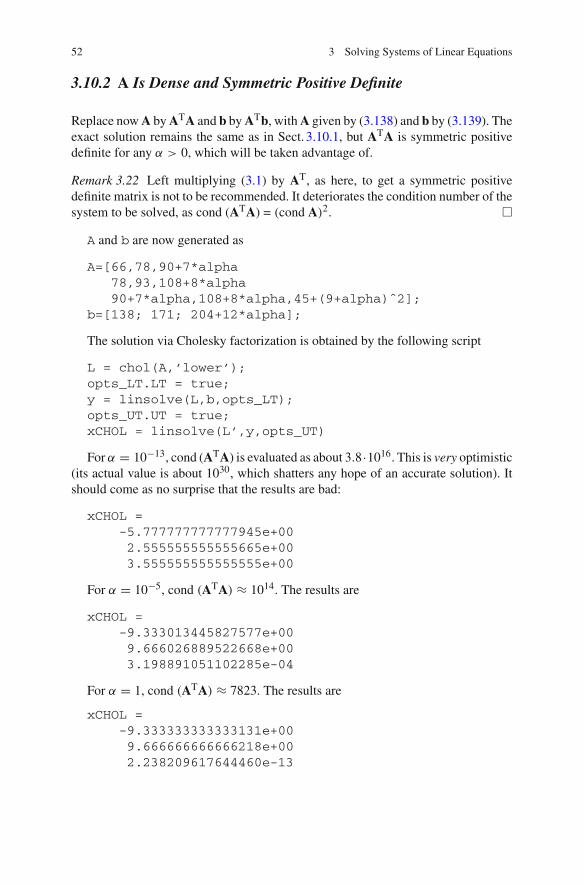
52 3 Solving Systems of Linear Equations

3.10.2 A Is Dense and Symmetric Positive Definite

Replace now A by ATA and b by ATb, with A given by (3.138) and b by (3.139). Theexact solution remains the same as in Sect. 3.10.1, but ATA is symmetric positivedefinite for any κ > 0, which will be taken advantage of.

Remark 3.22 Left multiplying (3.1) by AT, as here, to get a symmetric positivedefinite matrix is not to be recommended. It deteriorates the condition number of thesystem to be solved, as cond (ATA) = (cond A)2. �

A and b are now generated as

A=[66,78,90+7*alpha78,93,108+8*alpha90+7*alpha,108+8*alpha,45+(9+alpha)ˆ2];

b=[138; 171; 204+12*alpha];

The solution via Cholesky factorization is obtained by the following script

L = chol(A,’lower’);opts_LT.LT = true;y = linsolve(L,b,opts_LT);opts_UT.UT = true;xCHOL = linsolve(L’,y,opts_UT)

For κ = 10−13, cond (ATA) is evaluated as about 3.8·1016. This is very optimistic(its actual value is about 1030, which shatters any hope of an accurate solution). Itshould come as no surprise that the results are bad:

xCHOL =-5.777777777777945e+002.555555555555665e+003.555555555555555e+00

For κ = 10−5, cond (ATA) ≈ 1014. The results are

xCHOL =-9.333013445827577e+009.666026889522668e+003.198891051102285e-04

For κ = 1, cond (ATA) ≈ 7823. The results are

xCHOL =-9.333333333333131e+009.666666666666218e+002.238209617644460e-13

3.10 MATLAB Examples 53

3.10.3 A Is Sparse

A and sA, standing for the (asymmetric) sparse matrix A, are built by the script

n = 1.e3A = eye(n); % A is a 1000 by 1000 identity matrixA(1,n) = 1+alpha;A(n,1) = 1; % A now slightly modifiedsA = sparse(A);

Thus, dim x = 1000, and sA is a sparse representation of A where the zeros are notstored, whereas A is a dense representation of a sparse matrix, which comprises 106

entries, most of them being zeros. As in Sects. 3.10.1 and 3.10.2, A is singular forκ = 0, and its conditioning improves when κ increases.

All the entries of the vector b are taken equal to one, so b is built as

b = ones(n,1);

For any κ > 0, it is easy to check that the exact unique solution of (3.1) is then suchthat all its entries are equal to one, except for the last one, which is equal to zero. Thissystem has been solved with the same script as in the previous section for Gaussianelimination, LU factorization with partial pivoting, QR factorization and SVD, nottaking advantage of sparsity. For Krylov iteration, sA was used instead of A. Thefollowing script was employed to tune some optional parameters of gmres:

restart = 10;tol = 1e-12;maxit = 15;xKRY = gmres(sA,b,restart,tol,maxit);

(see the gmres documentation for details).For κ = 10−7, cond A ≈ 4 · 107 and the following results are obtained. The

time taken by each method is in s. As dim x = 1000, only the last two entries of thenumerical solution are provided. Recall that the first of them should be equal to oneand the last to zero.

TimeGE = 8.526009399999999e-02LastofxGE =

10

TimeLUP = 1.363140280000000e-01LastofxLUP =

10

54 3 Solving Systems of Linear Equations

TimeQR = 9.576683100000000e-02LastofxQR =

10

TimeSVD = 1.395477389000000e+00LastofxSVD =

10

gmres(10) converged at outer iteration 1(inner iteration 4)to a solution with relative residual 1.1e-21.TimeKRY = 9.034646100000000e-02LastofxKRY =

1.000000000000022e+001.551504706009954e-05

3.10.4 A Is Sparse and Symmetric Positive Definite

Consider the same example as in Sect. 3.10.3, but with n = 106, A replaced byATA and b replaced by ATb. sATA, standing for the sparse representation of the(symmetric positive definite) matrix ATA, may be built by

sATA = sparse(1:n,1:n,1); % sparse representation% of the (n,n) identity matrixsATA(1,1) = 2;sATA(1,n) = 2+alpha;sATA(n,1) = 2+alpha;sATA(n,n) = (1+alpha)ˆ2+1;

and ATb, standing for ATb, may be built by

ATb = ones(n,1);ATb(1) = 2;ATb(n) = 2+alpha;

(A dense representation of ATA would be unmanageable, with 1012 entries.)The (possibly preconditioned) conjugate gradient method is implemented in the

function pcg, which may be called as in

tol = 1e-15; % to be tunedxCG = pcg(sATA,ATb,tol);

3.10 MATLAB Examples 55

For κ = 10−3, cond (ATA) ≈ 1.6 · 107 and the following results are obtained. Asdim x = 106, only the last two entries of the numerical solution are provided. Recallthat the first of them should be equal to one and the last to zero.

pcg converged at iteration 6 to a solutionwith relative residual 2.2e-18.TimePCG = 5.922985430000000e-01LastofxPCG =

1-5.807653514112821e-09

3.11 In Summary

• Solving systems of linear equations plays a crucial role in almost all of themethods to be considered in what follows, and often takes up most of computingtime.

• Cramer’s method is not even an option.• Matrix inversion is uselessly costly, unless A has a very specific structure.• The larger the condition number of A is, the more difficult the problem becomes.• Solution via LU factorization is the basic workhorse to be used if A has no

particular structure to be taken advantage of. Pivoting makes it applicable forany nonsingular A. Although it increases the condition number of the problem,it does so with measure and may work just as well as QR factorization or SVDon ill-conditioned problems, for less computation.

• When the solution is not satisfactory, iterative correction may lead quickly to aspectacular improvement.

• Solution via QR factorization is more costly than via LU factorization but doesnot worsen conditioning. Orthonormal transformations play a central role in thisproperty.

• Solution via SVD, also based on orthonormal transformations, is even morecostly than via QR factorization. It has the advantage of providing the conditionnumber of A for the spectral norm as a by-product and of making it possible tofind approximate solutions to some hopelessly ill-conditioned problems throughregularization.

• Cholesky factorization is a special case of LU factorization, appropriate if A issymmetric and positive definite. It can also be used to test matrices for positivedefiniteness.

• When A is large and sparse, suitably preconditioned Krylov subspace iterationhas superseded classical iterative methods as it converges more quickly, moreoften.

56 3 Solving Systems of Linear Equations

• When A is large, sparse, symmetric and positive-definite, the conjugate-gradientapproach, a special case of Krylov subspace iteration, is the method of choice.

• When dealing with large, sparse matrices, a suitable reindexation of the nonzeroentries may speed up computation by several orders of magnitude.

References

1. Golub, G., Van Loan, C.: Matrix Computations, 3rd edn. The Johns Hopkins University Press,Baltimore (1996)

2. Demmel, J.: Applied Numerical Linear Algebra. SIAM, Philadelphia (1997)3. Ascher, U., Greif, C.: A First Course in Numerical Methods. SIAM, Philadelphia (2011)4. Rice, J.: A theory of condition. SIAM J. Numer. Anal. 3(2), 287–310 (1966)5. Demmel, J.: The probability that a numerical analysis problem is difficult. Math. Comput.

50(182), 449–480 (1988)6. Higham, N.: Fortran codes for estimating the one-norm of a real or complex matrix, with

applications to condition estimation (algorithm 674). ACM Trans. Math. Softw. 14(4), 381–396 (1988)

7. Higham, N., Tisseur, F.: A block algorihm for matrix 1-norm estimation, with an applicationto 1-norm pseudospectra. SIAM J. Matrix Anal. Appl. 21, 1185–1201 (2000)

8. Higham, N.: Gaussian elimination. Wiley Interdiscip. Rev. Comput. Stat. 3(3), 230–238 (2011)9. Stewart, G.: The decomposition approach to matrix computation. Comput. Sci. Eng. 2(1),

50–59 (2000)10. Björck, A.: Numerical Methods for Least Squares Problems. SIAM, Philadelphia (1996)11. Golub G, Kahan W.: Calculating the singular values and pseudo-inverse of a matrix. J. Soc.

Indust. Appl. Math. Ser. B Numer. Anal. 2(2), 205–224 (1965)12. Stewart, G.: On the early history of the singular value decomposition. SIAM Rev. 35(4), 551–

566 (1993)13. Varah, J.: On the numerical solution of ill-conditioned linear systems with applications to

ill-posed problems. SIAM J. Numer. Anal. 10(2), 257–267 (1973)14. Saad, Y.: Iterative Methods for Sparse Linear Systems, 2nd edn. SIAM, Philadelphia (2003)15. Young, D.: Iterative methods for solving partial difference equations of elliptic type. Ph.D.

thesis, Harvard University, Cambridge, MA (1950)16. Gutknecht, M.: A brief introduction to Krylov space methods for solving linear systems. In: Y.

Kaneda, H. Kawamura, M. Sasai (eds.) Proceedings of International Symposium on Frontiersof Computational Science 2005, pp. 53–62. Springer, Berlin (2007)

17. van der Vorst, H.: Krylov subspace iteration. Comput. Sci. Eng. 2(1), 32–37 (2000)18. Dongarra, J., Sullivan, F.: Guest editors’ introduction to the top 10 algorithms. Comput. Sci.

Eng. 2(1), 22–23 (2000)19. Hestenes, M., Stiefel, E.: Methods of conjugate gradients for solving linear systems. J. Res.

Natl. Bur. Stan 49(6), 409–436 (1952)20. Golub, G., O’Leary, D.: Some history of the conjugate gradient and Lanczos algorithms: 1948–

1976. SIAM Rev. 31(1), 50–102 (1989)21. Shewchuk, J.: An introduction to the conjugate gradient method without the agonizing pain.

Technical report, School of Computer Science. Carnegie Mellon University, Pittsburgh (1994)22. Paige, C., Saunders, M.: Solution of sparse indefinite systems of linear equations. SIAM J.

Numer. Anal. 12(4), 617–629 (1975)23. Saad, Y., Schultz, M.: GMRES: a generalized minimal residual algorithm for solving nonsym-

metric linear systems. SIAM J. Sci. Stat. Comput. 7(3), 856–869 (1986)24. van der Vorst, H.: Bi-CGSTAB: a fast and smoothly convergent variant of Bi-CG for the solution

of nonsymmetric linear systems. SIAM J. Sci. Stat. Comput. 13(2), 631–644 (1992)

References 57

25. Benzi, M.: Preconditioning techniques for large linear systems: a survey. J. Comput. Phys. 182,418–477 (2002)

26. Saad, Y.: Preconditioning techniques for nonsymmetric and indefinite linear systems. J. Com-put. Appl. Math. 24, 89–105 (1988)

27. Grote, M., Huckle, T.: Parallel preconditioning with sparse approximate inverses. SIAM J. Sci.Comput. 18(3), 838–853 (1997)

28. Higham, N.: Cholesky factorization. Wiley Interdiscip. Rev. Comput. Stat. 1(2), 251–254(2009)

29. Ciarlet, P.: Introduction to Numerical Linear Algebra and Optimization. Cambridge UniversityPress, Cambridge (1989)

30. Gilbert, J., Moler, C., Schreiber, R.: Sparse matrices in MATLAB: design and implementation.SIAM J. Matrix Anal. Appl. 13, 333–356 (1992)

Chapter 4Solving Other Problems in Linear Algebra

This chapter is about the evaluation of the inverse, determinant, eigenvalues, andeigenvectors of an (n × n) matrix A.

4.1 Inverting Matrices

Before evaluating the inverse of a matrix, check that the actual problem is notrather solving a system of linear equations (see Chap. 3).

Unless A has a very specific structure, such as being diagonal, it is usually invertedby solving

AA−1 = In (4.1)

for A−1. This is equivalent to solving the n linear systems

Axi = ei , i = 1, . . . , n, (4.2)

with xi the i th column of A−1 and ei the i th column of In .

Remark 4.1 Since the n systems (4.2) share the same matrix A, any LU or QRfactorization needs to be carried out only once. With LU factorization, for instance,inverting a dense (n ×n) matrix A requires about 8n3/3 flops, when solving Ax = bcosts only about

[⎡2n3/3

⎢ + 2n2⎣

flops. �

For LU factorization with partial pivoting, solving (4.2) means solving the trian-gular systems

Lyi = Pei , i = 1, . . . , n, (4.3)

É. Walter, Numerical Methods and Optimization, 59DOI: 10.1007/978-3-319-07671-3_4,© Springer International Publishing Switzerland 2014

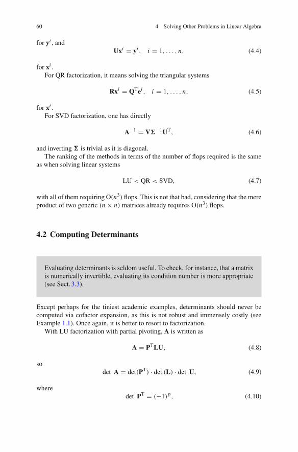
60 4 Solving Other Problems in Linear Algebra

for yi , andUxi = yi , i = 1, . . . , n, (4.4)

for xi .

For QR factorization, it means solving the triangular systems

Rxi = QTei , i = 1, . . . , n, (4.5)

for xi .

For SVD factorization, one has directly

A−1 = V�−1UT, (4.6)

and inverting � is trivial as it is diagonal.The ranking of the methods in terms of the number of flops required is the same

as when solving linear systems

LU < QR < SVD, (4.7)

with all of them requiring O(n3) flops. This is not that bad, considering that the mereproduct of two generic (n × n) matrices already requires O(n3) flops.

4.2 Computing Determinants

Evaluating determinants is seldom useful. To check, for instance, that a matrixis numerically invertible, evaluating its condition number is more appropriate(see Sect. 3.3).

Except perhaps for the tiniest academic examples, determinants should never becomputed via cofactor expansion, as this is not robust and immensely costly (seeExample 1.1). Once again, it is better to resort to factorization.

With LU factorization with partial pivoting, A is written as

A = PTLU, (4.8)

sodet A = det(PT) · det (L) · det U, (4.9)

wheredet PT = (−1)p, (4.10)

4.2 Computing Determinants 61

with p the number of row exchanges due to pivoting, where

det L = 1 (4.11)

and where det U is the product of the diagonal entries of U.With QR factorization, A is written as

A = QR, (4.12)

sodet A = det (Q) · det R. (4.13)

Equation (3.64) implies thatdet Q = (−1)q , (4.14)

where q is the number of Householder transformations, and det R is equal to theproduct of the diagonal entries of R.

With SVD, A is written asA = U�VT, (4.15)

sodet A = det(U) · det(�) · det VT. (4.16)

Now det U = ±1, det VT = ±1 and det � = ⎤ni=1 σi,i .

4.3 Computing Eigenvalues and Eigenvectors

4.3.1 Approach Best Avoided

The eigenvalues of the (square) matrix A are the solutions for λ of the characteristicequation

det (A − λI) = 0, (4.17)

and the eigenvector vi associated with the eigenvalue λi satisfies

Avi = λi vi , (4.18)

which defines it up to an arbitrary nonzero multiplicative constant.One may think of a three-stage procedure, where the coefficients of the polynomial

equation (4.17) would be evaluated from A, before using some general-purposealgorithm for solving (4.17) for λ and solving the linear system (4.18) for vi for eachof the λi ’s thus computed. Unless the problem is very small, this is a bad idea, if

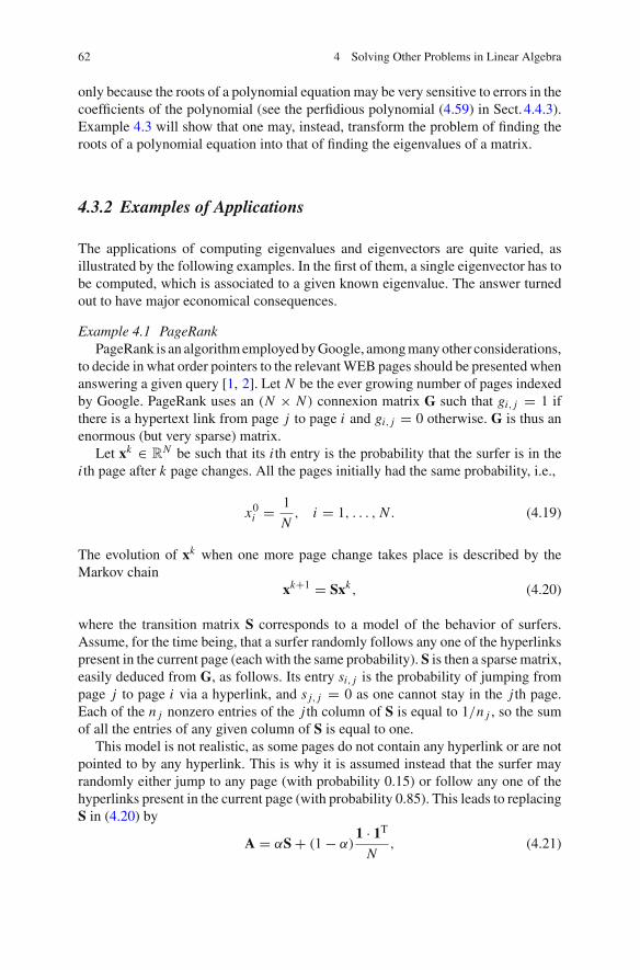
62 4 Solving Other Problems in Linear Algebra

only because the roots of a polynomial equation may be very sensitive to errors in thecoefficients of the polynomial (see the perfidious polynomial (4.59) in Sect. 4.4.3).Example 4.3 will show that one may, instead, transform the problem of finding theroots of a polynomial equation into that of finding the eigenvalues of a matrix.

4.3.2 Examples of Applications

The applications of computing eigenvalues and eigenvectors are quite varied, asillustrated by the following examples. In the first of them, a single eigenvector has tobe computed, which is associated to a given known eigenvalue. The answer turnedout to have major economical consequences.

Example 4.1 PageRankPageRank is an algorithm employed by Google, among many other considerations,

to decide in what order pointers to the relevant WEB pages should be presented whenanswering a given query [1, 2]. Let N be the ever growing number of pages indexedby Google. PageRank uses an (N × N ) connexion matrix G such that gi, j = 1 ifthere is a hypertext link from page j to page i and gi, j = 0 otherwise. G is thus anenormous (but very sparse) matrix.

Let xk √ RN be such that its i th entry is the probability that the surfer is in the

i th page after k page changes. All the pages initially had the same probability, i.e.,

x0i = 1

N, i = 1, . . . , N . (4.19)

The evolution of xk when one more page change takes place is described by theMarkov chain

xk+1 = Sxk, (4.20)

where the transition matrix S corresponds to a model of the behavior of surfers.Assume, for the time being, that a surfer randomly follows any one of the hyperlinkspresent in the current page (each with the same probability). S is then a sparse matrix,easily deduced from G, as follows. Its entry si, j is the probability of jumping frompage j to page i via a hyperlink, and s j, j = 0 as one cannot stay in the j th page.Each of the n j nonzero entries of the j th column of S is equal to 1/n j , so the sumof all the entries of any given column of S is equal to one.

This model is not realistic, as some pages do not contain any hyperlink or are notpointed to by any hyperlink. This is why it is assumed instead that the surfer mayrandomly either jump to any page (with probability 0.15) or follow any one of thehyperlinks present in the current page (with probability 0.85). This leads to replacingS in (4.20) by

A = αS + (1 − α)1 · 1T

N, (4.21)

4.3 Computing Eigenvalues and Eigenvectors 63

with α = 0.85 and 1 an N -dimensional column vector full of ones. With this model,the probability of staying at the same page is no longer zero, but this makes evaluatingAxk almost as simple as if A were sparse; see Sect. 16.1.

After an infinite number of clicks, the asymptotic distribution of probabilities x∇satisfies

Ax∇ = x∇, (4.22)

so x∇ is an eigenvector of A, associated with a unit eigenvalue. Eigenvectors aredefined up to a multiplicative constant, but the meaning of x∇ implies that

N⎥

i=1

x∇i = 1. (4.23)

Once x∇ has been evaluated, the relevant pages with the highest values of their entryin x∇ are presented first. The transition matrices of Markov chains are such that theireigenvalue with the largest magnitude is equal to one. Ranking WEB pages thus boilsdown to computing the eigenvector associated with the (known) eigenvalue with thelargest magnitude of a tremendously large (and almost sparse) matrix. �Example 4.2 Bridge oscillations

On the morning of November 7, 1940, the Tacoma Narrows bridge twisted vio-lently in the wind before collapsing into the cold waters of the Puget Sound. Thebridge had earned the nickname Galloping Gertie for its unusual behavior, and itis an extraordinary piece of luck that no thrill-seeker was killed in the disaster. Thevideo of the event, available on the WEB, is a stark reminder of the importance oftaking potential oscillations into account during bridge design.

A linear dynamical model of a bridge, valid for small displacements, is given bythe vector ordinary differential equation

Mx + Cx + Kx = u, (4.24)

with M a matrix of masses, C a matrix of damping coefficients, K a matrix ofstiffness coefficients, x a vector describing the displacements of the nodes of a meshwith respect to their equilibrium position in the absence of external forces and u avector of external forces. C is often negligible, which is one of the main reasonswhy oscillations are so dangerous. In the absence of external input, the autonomousequation is then

Mx + Kx = 0. (4.25)

All the solutions of this equation are linear combinations of proper modes xk , with

xk(t) = ρρρk exp[i(ωk t + ϕk)], (4.26)

where i is the imaginary unit, such that i2 = −1, ωk is a resonant angular frequencyand ρρρk is the associated mode shape. Plug (4.26) into (4.25) to get

64 4 Solving Other Problems in Linear Algebra

(K − ω2k M)ρρρk = 0. (4.27)

Computing ω2k and ρρρk is known as a generalized eigenvalue problem [3]. Usually,

M is invertible, so this equation can be transformed into

Aρρρk = λkρρρk, (4.28)

with λk = ω2k and A = M−1K. Computing the ωk’s and ρρρk’s thus boils down to

computing eigenvalues and eigenvectors, although solving the initial generalizedeigenvalue problem as such may actually be a better idea, as useful properties of Mand K may be lost when computing M−1K. �Example 4.3 Solving a polynomial equation

The roots of the polynomial equation

xn + an−1xn−1 + · · · + a1x + a0 = 0 (4.29)

are the eigenvalues of its companion matrix

A =

⎦

⎞⎞⎞⎞⎞⎞⎞⎞⎞⎞⎞⎞⎠

0 · · · · · · 0 −a0

1. . . 0

... −a1

0. . .

. . ....

...

.... . .

. . . 0...

0 · · · 0 1 −an−1

, (4.30)

and one of the most efficient methods for computing these roots is to look for theeigenvalues of A. �

4.3.3 Power Iteration

The power iteration method applies when the eigenvalue of A with the largest mag-nitude is real and simple. It then computes this eigenvalue and the correspondingeigenvector. Its main use is on large matrices that are sparse (or can be treated as ifthey were sparse, as in PageRank).

Assume, for the time being, that the eigenvalue λmax with the largest magni-tude is positive. Provided that v0 has a nonzero component in the direction of thecorresponding eigenvector vmax, iterating

vk+1 = Avk (4.31)

4.3 Computing Eigenvalues and Eigenvectors 65

will then decrease the angle between vk and vmax at each iteration. To ensure that∥∥vk+1∥∥

2 = 1, (4.31) is replaced by

vk+1 = 1∥∥Avk∥∥

2

Avk . (4.32)

Upon convergence,Av∇ = ∥∥Av∇∥∥

2 v∇, (4.33)

so λmax = ∥∥Av∇∥∥2 and vmax = v∇. Convergence may be slow if other eigenvalues

are close in magnitude to λmax.

Remark 4.2 When λmax is negative, the method becomes

vk+1 = − 1∥∥Avk∥∥

2

Avk, (4.34)

so that upon convergenceAv∇ = − ∥∥Av∇∥∥

2 v∇. (4.35)

�

Remark 4.3 If A is symmetric, then its eigenvectors are orthogonal and, providedthat →vmax→2 = 1, the matrix

A⇒ = A − λmaxvmaxvTmax (4.36)

has the same eigenvalues and eigenvectors as A, except for vmax, which is nowassociated with λ = 0. One may thus apply power iterations to find the eigenvaluewith the second largest magnitude and the corresponding eigenvector. This deflationprocedure should be iterated with caution, as errors cumulate. �

4.3.4 Inverse Power Iteration

When A is invertible and has a unique real eigenvalue λmin with smallest magnitude,the eigenvalue of A−1 with the largest magnitude is 1

λmin, so an inverse power iteration

vk+1 = 1∥∥A−1vk∥∥

2

A−1vk (4.37)

might be used to compute λmin and the corresponding eigenvector (provided thatλmin > 0). Inverting A is avoided by solving the system

66 4 Solving Other Problems in Linear Algebra

Avk+1 = vk (4.38)

for vk+1 and normalizing the result. If a factorization of A is used for this purpose,it needs to be carried out only once. A trivial modification of the algorithm makes itpossible to deal with the case λmin < 0.

4.3.5 Shifted Inverse Power Iteration

Shifted inverse power iteration aims at computing an eigenvector xi associated withsome approximately known isolated eigenvalue λi , which need not be the one withthe largest or smallest magnitude. It can be used on real or complex matrices, andis particularly efficient on normal matrices, i.e., matrices A that commute with theirtransconjugate AH:

AAH = AHA. (4.39)

For real matrices, this translates into

AAT = ATA, (4.40)

so symmetric real matrices are normal.Let ρ be an approximate value for λi , with ρ ∈= λi . Since

Axi = λi xi , (4.41)

we have(A − ρI)xi = (λi − ρ)xi . (4.42)

Multiply (4.42) on the left by (A − ρI)−1(λi − ρ)−1, to get

(A − ρI)−1xi = (λi − ρ)−1xi . (4.43)

The vector xi is thus also an eigenvector of (A−ρI)−1, associated with the eigenvalue(λi −ρ)−1. By choosing ρ close enough to λi , and provided that the other eigenvaluesof A are far enough, one can ensure that, for all j ∈= i ,

1

|λi − ρ| � 1

|λ j − ρ| . (4.44)

Shifted inverse power iteration

vk+1 = (A − ρI)−1vk, (4.45)

4.3 Computing Eigenvalues and Eigenvectors 67

combined with a normalization of vk+1 at each step, then converges to an eigenvectorof A associated with λi . In practice, of course, one rather solves

(A − ρI)vk+1 = vk (4.46)

for vk+1 (usually via an LU factorization with partial pivoting of (A − ρI), whichneeds to be carried out only once). When ρ gets close to λi , the matrix (A − ρI)becomes nearly singular, but the algorithm works nevertheless very well, at leastwhen A is normal. Its properties, including its behavior on non-normal matrices, areinvestigated in [4].

4.3.6 QR Iteration

QR iteration, based on QR factorization, makes it possible to compute all the eigen-values of a not too large and possibly dense matrix A with real coefficients. Theseeigenvalues may be real or complex-conjugate. It is only assumed that their mag-nitude differ (except, of course, for a pair of complex-conjugate eigenvalues). Aninteresting account of the history of this fascinating algorithm can be found in [5].Its convergence is studied in [6].

The basic method is as follows. Starting with A0 = A and i = 0, repeat untilconvergence

1. Factor Ai as Qi Ri .2. Invert the order of the resulting factors Qi and Ri to get Ai+1 = Ri Qi .3. Increment i by one and go to Step 1.

For reasons not trivial to explain, this transfers mass from the lower triangular partof Ai to the upper triangular part of Ai+1. The fact that Ri = Q−1

i Ai implies thatAi+1 = Q−1

i Ai Qi . The matrices Ai+1 and Ai therefore have the same eigenvalues.Upon convergence, A∇ is a block upper triangular matrix with the same eigenvaluesas A, in what is called a real Schur form. There are only (1×1) and (2 ×2) diagonalblocks in A∇. Each (1 × 1) block contains a real eigenvalue of A, whereas theeigenvalues of the (2 × 2) blocks are complex-conjugate eigenvalues of A. If Bis one such (2 × 2) block, then its eigenvalues are the roots of the second-orderpolynomial equation

λ2 − trace (B) λ + det B = 0. (4.47)

The resulting factorizationA = QA∇QT (4.48)

is called a (real) Schur decomposition. Since

Q =∏

i

Qi , (4.49)

68 4 Solving Other Problems in Linear Algebra

it is orthonormal, as the product of orthonormal matrices, and (4.48) implies that

A = QA∇Q−1. (4.50)

Remark 4.4 After pointing out that “good implementations [of the QR algorithm]have long been much more widely available than good explanations”, [7] shows thatthe QR algorithm is just a clever and numerically robust implementation of the poweriteration method of Sect. 4.3.3 applied to an entire basis of Rn rather than to a singlevector. �

Remark 4.5 Whenever A is not an upper Hessenberg matrix (i.e., an upper triangularmatrix completed with an additional nonzero descending diagonal just below themain descending diagonal), a trivial variant of the QR algorithm is used first to putit into this form. This speeds up QR iteration considerably, as the upper Hessenbergform is preserved by the iterations. Note that the companion matrix of Example 4.3is already in upper Hessenberg form. �

If A is symmetric, then all the eigenvalues λi (i = 1, . . . , n) of A are real, and thecorresponding eigenvectors vi are orthogonal. QR iteration then produces a series ofsymmetric matrices Ak that should converge to the diagonal matrix

� = Q−1AQ, (4.51)

with Q orthonormal and

� =

⎦

⎞⎞⎞⎞⎠

λ1 0 · · · 0

0 λ2. . .

......

. . .. . . 0

0 · · · 0 λn

. (4.52)

Equation (4.51) implies thatAQ = Q�, (4.53)

or, equivalently,Aqi = λi qi , i = 1, . . . , n, (4.54)

where qi is the i th column of Q. Thus, qi is the eigenvector associated with λi , andthe QR algorithm computes the spectral decomposition of A

A = Q�QT. (4.55)

When A is not symmetric, computing its eigenvectors from the Schur decompo-sition becomes significantly more complicated; see, e.g., [8].

4.3 Computing Eigenvalues and Eigenvectors 69

4.3.7 Shifted QR Iteration

The basic version of QR iteration fails if there are several real eigenvalues (or severalpairs of complex-conjugate eigenvalues) with the same magnitude, as illustrated bythe following example.

Example 4.4 Failure of QR iterationThe QR factorization of

A =[

0 11 0

],

is

A =[

0 11 0

]·

[1 00 1

],

soRQ = A

and the method is stuck. This is not surprising as the eigenvalues of A have the sameabsolute value (λ1 = 1 and λ2 = −1). �

To bypass this difficulty and speed up convergence, the basic shifted QR methodproceeds as follows. Starting with A0 = A and i = 0, it repeats until convergence

1. Choose a shift σi .2. Factor Ai − σi I as Qi Ri .3. Invert the order of the resulting factors Qi and Ri and compensate the shift, to

get Ai+1 = Ri Qi + σi I.

A possible strategy is as follows. First set σi to the value of the last diagonalentry of Ai , to speed up convergence of the last row, then set σi to the value of thepenultimate diagonal entry of Ai , to speed up convergence of the penultimate row,and so on.

Much work has been carried out on the theoretical properties and details of theimplementation of (shifted) QR iteration, and its surface has only been scratchedhere. QR iteration, which has been dubbed one of the most remarkable algorithmsin numerical mathematics ([9], quoted in [8]), turns out to converge in more generalsituations than those for which its convergence has been proven. It has, however,two main drawbacks. First, the eigenvalues with small magnitudes may be evaluatedwith insufficient precision, which may justify iterative improvement, for instance by(shifted) inverse power iteration. Second, the QR algorithm is not suited for verylarge, sparse matrices, as it destroys sparsity. On the numerical solution of largeeigenvalue problems, the reader may consult [3], and discover that Krylov subspacesonce again play a crucial role.

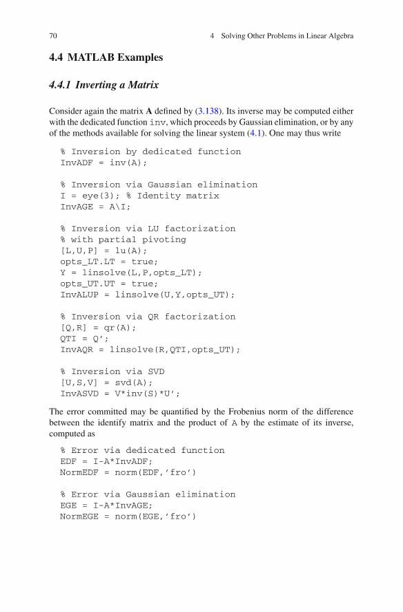
70 4 Solving Other Problems in Linear Algebra

4.4 MATLAB Examples

4.4.1 Inverting a Matrix

Consider again the matrix A defined by (3.138). Its inverse may be computed eitherwith the dedicated function inv, which proceeds by Gaussian elimination, or by anyof the methods available for solving the linear system (4.1). One may thus write

% Inversion by dedicated functionInvADF = inv(A);

% Inversion via Gaussian eliminationI = eye(3); % Identity matrixInvAGE = A\I;

% Inversion via LU factorization% with partial pivoting[L,U,P] = lu(A);opts_LT.LT = true;Y = linsolve(L,P,opts_LT);opts_UT.UT = true;InvALUP = linsolve(U,Y,opts_UT);

% Inversion via QR factorization[Q,R] = qr(A);QTI = Q’;InvAQR = linsolve(R,QTI,opts_UT);

% Inversion via SVD[U,S,V] = svd(A);InvASVD = V*inv(S)*U’;

The error committed may be quantified by the Frobenius norm of the differencebetween the identify matrix and the product of A by the estimate of its inverse,computed as

% Error via dedicated functionEDF = I-A*InvADF;NormEDF = norm(EDF,’fro’)

% Error via Gaussian eliminationEGE = I-A*InvAGE;NormEGE = norm(EGE,’fro’)

4.4 MATLAB Examples 71

% Error via LU factorization% with partial pivotingELUP = I-A*InvALUP;NormELUP = norm(ELUP,’fro’)

% Error via QR factorizationEQR = I-A*InvAQR;NormEQR = norm(EQR,’fro’)

% Error via SVDESVD = I-A*InvASVD;NormESVD = norm(ESVD,’fro’)

For α = 10−13,

NormEDF = 3.685148879709611e-02NormEGE = 1.353164693413185e-02NormELUP = 1.353164693413185e-02NormEQR = 3.601384553630034e-02NormESVD = 1.732896329126472e-01

For α = 10−5,

NormEDF = 4.973264728508383e-10NormEGE = 2.851581367178794e-10NormELUP = 2.851581367178794e-10NormEQR = 7.917097832969996e-10NormESVD = 1.074873453042201e-09

Once again, LU factorization with partial pivoting thus turns out to be a very goodchoice on this example, as it achieves the lowest error norm with the least numberof flops.

4.4.2 Evaluating a Determinant

We take advantage here of the fact that the determinant of the matrix A definedby (3.138) is equal to −3α. If detX is the numerical value of the determinant ascomputed by the method X, we compute the relative error of this method as

TrueDet = -3*alpha;REdetX = (detX-TrueDet)/TrueDet

The determinant of A may be computed either by the dedicated function det, as

detDF = det(A);

or by evaluating the product of the determinants of the matrices of an LUP, QR, orSVD factorization.

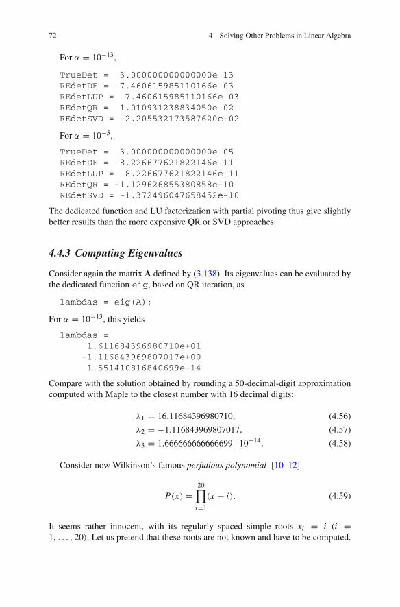
72 4 Solving Other Problems in Linear Algebra

For α = 10−13,

TrueDet = -3.000000000000000e-13REdetDF = -7.460615985110166e-03REdetLUP = -7.460615985110166e-03REdetQR = -1.010931238834050e-02REdetSVD = -2.205532173587620e-02

For α = 10−5,

TrueDet = -3.000000000000000e-05REdetDF = -8.226677621822146e-11REdetLUP = -8.226677621822146e-11REdetQR = -1.129626855380858e-10REdetSVD = -1.372496047658452e-10

The dedicated function and LU factorization with partial pivoting thus give slightlybetter results than the more expensive QR or SVD approaches.

4.4.3 Computing Eigenvalues

Consider again the matrix A defined by (3.138). Its eigenvalues can be evaluated bythe dedicated function eig, based on QR iteration, as

lambdas = eig(A);

For α = 10−13, this yields

lambdas =1.611684396980710e+01-1.116843969807017e+001.551410816840699e-14

Compare with the solution obtained by rounding a 50-decimal-digit approximationcomputed with Maple to the closest number with 16 decimal digits:

λ1 = 16.11684396980710, (4.56)

λ2 = −1.116843969807017, (4.57)

λ3 = 1.666666666666699 · 10−14. (4.58)

Consider now Wilkinson’s famous perfidious polynomial [10–12]

P(x) =20∏

i=1

(x − i). (4.59)

It seems rather innocent, with its regularly spaced simple roots xi = i (i =1, . . . , 20). Let us pretend that these roots are not known and have to be computed.

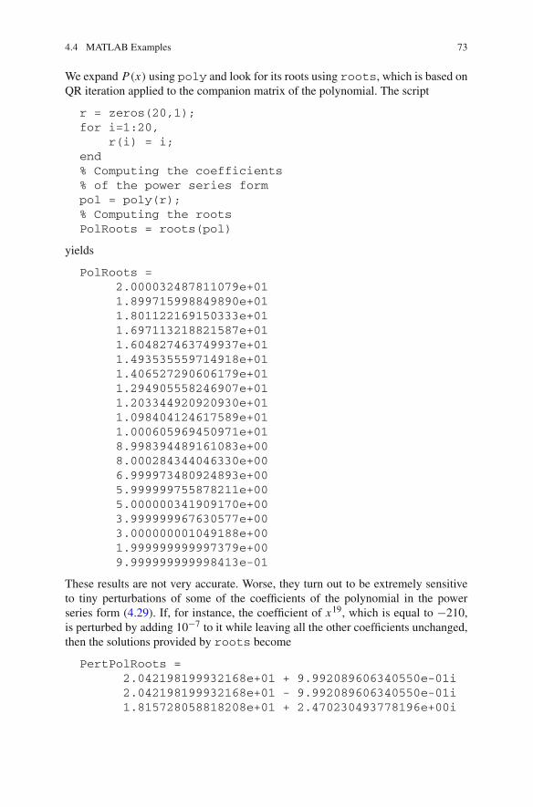
4.4 MATLAB Examples 73

We expand P(x) using poly and look for its roots using roots, which is based onQR iteration applied to the companion matrix of the polynomial. The script

r = zeros(20,1);for i=1:20,

r(i) = i;end% Computing the coefficients% of the power series formpol = poly(r);% Computing the rootsPolRoots = roots(pol)

yields

PolRoots =2.000032487811079e+011.899715998849890e+011.801122169150333e+011.697113218821587e+011.604827463749937e+011.493535559714918e+011.406527290606179e+011.294905558246907e+011.203344920920930e+011.098404124617589e+011.000605969450971e+018.998394489161083e+008.000284344046330e+006.999973480924893e+005.999999755878211e+005.000000341909170e+003.999999967630577e+003.000000001049188e+001.999999999997379e+009.999999999998413e-01

These results are not very accurate. Worse, they turn out to be extremely sensitiveto tiny perturbations of some of the coefficients of the polynomial in the powerseries form (4.29). If, for instance, the coefficient of x19, which is equal to −210,is perturbed by adding 10−7 to it while leaving all the other coefficients unchanged,then the solutions provided by roots become

PertPolRoots =2.042198199932168e+01 + 9.992089606340550e-01i2.042198199932168e+01 - 9.992089606340550e-01i1.815728058818208e+01 + 2.470230493778196e+00i

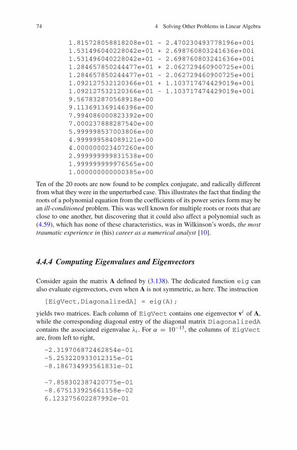
74 4 Solving Other Problems in Linear Algebra

1.815728058818208e+01 - 2.470230493778196e+00i1.531496040228042e+01 + 2.698760803241636e+00i1.531496040228042e+01 - 2.698760803241636e+00i1.284657850244477e+01 + 2.062729460900725e+00i1.284657850244477e+01 - 2.062729460900725e+00i1.092127532120366e+01 + 1.103717474429019e+00i1.092127532120366e+01 - 1.103717474429019e+00i9.567832870568918e+009.113691369146396e+007.994086000823392e+007.000237888287540e+005.999998537003806e+004.999999584089121e+004.000000023407260e+002.999999999831538e+001.999999999976565e+001.000000000000385e+00

Ten of the 20 roots are now found to be complex conjugate, and radically differentfrom what they were in the unperturbed case. This illustrates the fact that finding theroots of a polynomial equation from the coefficients of its power series form may bean ill-conditioned problem. This was well known for multiple roots or roots that areclose to one another, but discovering that it could also affect a polynomial such as(4.59), which has none of these characteristics, was in Wilkinson’s words, the mosttraumatic experience in (his) career as a numerical analyst [10].

4.4.4 Computing Eigenvalues and Eigenvectors

Consider again the matrix A defined by (3.138). The dedicated function eig canalso evaluate eigenvectors, even when A is not symmetric, as here. The instruction

[EigVect,DiagonalizedA] = eig(A);

yields two matrices. Each column of EigVect contains one eigenvector vi of A,while the corresponding diagonal entry of the diagonal matrix DiagonalizedAcontains the associated eigenvalue λi . For α = 10−13, the columns of EigVectare, from left to right,

-2.319706872462854e-01-5.253220933012315e-01-8.186734993561831e-01

-7.858302387420775e-01-8.675133925661158e-026.123275602287992e-01

4.4 MATLAB Examples 75

4.082482904638510e-01-8.164965809277283e-014.082482904638707e-01

The diagonal entries of DiagonalizedA are, in the same order,

1.611684396980710e+01-1.116843969807017e+001.551410816840699e-14

They are thus identical to the eigenvalues previously obtained with the instructioneig(A).

A (very partial) check of the quality of these results can be carried out with thescript

Residual = A*EigVect-EigVect*DiagonalizedA;NormResidual = norm(Residual,’fro’)

which yields

NormResidual = 1.155747735077462e-14

4.5 In Summary

• Think twice before inverting a matrix. You may just want to solve a system oflinear equations.

• When necessary, the inversion of an (n × n) matrix can be carried out by solvingn systems of n linear equations in n unknowns. If an LU or QR factorization of Ais used, then it needs to be performed only once.

• Think twice before evaluating a determinant. You may be more interested in acondition number.

• Computing the determinant of A is easy from an LU or QR factorization of A. Theresult based on QR factorization requires more computation but should be morerobust to ill conditioning.

• Power iteration can be used to compute the eigenvalue of A with the largest mag-nitude, provided that it is real and unique, and the corresponding eigenvector. Itis particularly interesting when A is large and sparse. Variants of power iterationcan be used to compute the eigenvalue of A with the smallest magnitude and thecorresponding eigenvector, or the eigenvector associated with any approximatelyknown isolated eigenvalue.

• (Shifted) QR iteration is the method of choice for computing all the eigenvalues ofA simultaneously. It can also be used to compute the corresponding eigenvectors,which is particularly easy if A is symmetric.

• (Shifted) QR iteration can also be used for simultaneously computing all theroots of a polynomial equation in a single indeterminate. The results may be verysensitive to the values of the coefficients of the polynomial in power series form.

76 4 Solving Other Problems in Linear Algebra

References

1. Langville, A., Meyer, C.: Google’s PageRank and Beyond. Princeton University Press, Prince-ton (2006)

2. Bryan, K., Leise, T.: The $25,000,000,000 eigenvector: the linear algebra behind Google. SIAMRev. 48(3), 569–581 (2006)

3. Saad, Y.: Numerical Methods for Large Eigenvalue Problems, 2nd edn. SIAM, Philadelphia(2011)

4. Ipsen, I.: Computing an eigenvector with inverse iteration. SIAM Rev. 39, 254–291 (1997)5. Parlett, B.: The QR algorithm. Comput. Sci. Eng. 2(1), 38–42 (2000)6. Wilkinson, J.: Convergence of the LR, QR, and related algorithms. Comput. J. 8, 77–84 (1965)7. Watkins, D.: Understanding the QR algorithm. SIAM Rev. 24(4), 427–440 (1982)8. Ciarlet, P.: Introduction to Numerical Linear Algebra and Optimization. Cambridge University

Press, Cambridge (1989)9. Strang, G.: Introduction to Applied Mathematics. Wellesley-Cambridge Press, Wellesley

(1986)10. Wilkinson, J.: The perfidious polynomial. In: Golub, G. (Ed.) Studies in Numerical Analysis,

Studies in Mathematics vol. 24, pp. 1–28. Mathematical Association of America, Washington,DC (1984)

11. Acton, F.: Numerical Methods That (Usually) Work, revised edn. Mathematical Associationof America, Washington, DC (1990)

12. Farouki, R.: The Bernstein polynomial basis: a centennial retrospective. Comput. Aided Geom.Des. 29, 379–419 (2012)

Chapter 5Interpolating and Extrapolating

5.1 Introduction

Consider a function f(·) such that

y = f(x), (5.1)

with x a vector of inputs and y a vector of outputs, and assume it is a black box, i.e., itcan only be evaluated numerically and nothing is known about its formal expression.Assume further that f(·) has been evaluated at N different numerical values xi of x,so the N corresponding numerical values of the output vector

yi = f(xi ), i = 1, . . . , N , (5.2)

are known. Let g(·) be another function, usually much simpler to evaluate than f(·),and such that

g(xi ) = f(xi ), i = 1, . . . , N . (5.3)

Computing g(x) is called interpolation if x is inside the convex hull of the xi ’s,i.e., the smallest convex polytope that contains all of them. Otherwise, one speaksof extrapolation (Fig. 5.1). A must read on interpolation (and approximation) withpolynomial and rational functions is [1]; see also the delicious [2].

Although the methods developed for interpolation can also be used for extrap-olation, the latter is much more dangerous. When at all possible, it shouldtherefore be avoided by enclosing the domain of interest in the convex hull ofthe xi ’s.

Remark 5.1 It is not always a good idea to interpolate, if only because the data yi

are often corrupted by noise. It is sometimes preferable to get a simpler model that

É. Walter, Numerical Methods and Optimization, 77DOI: 10.1007/978-3-319-07671-3_5,© Springer International Publishing Switzerland 2014

78 5 Interpolating and Extrapolating

Interpolation

Extrapolation

x4

x1

x2

x3

x5

Fig. 5.1 Extrapolation takes place outside the convex hull of the xi ’s

satisfiesg(xi ) √ f(xi ), i = 1, . . . , N . (5.4)

This model may deliver much better predictions of y at x ∇= xi than an interpolatingmodel. Its optimal construction will be considered in Chap. 9. �

5.2 Examples

Example 5.1 Computer experimentsActual experiments in the physical world are increasingly being replaced by

numerical computation. To design cars that meet safety norms during crashes, forinstance, manufacturers have partly replaced the long and costly actual crashing ofprototypes by numerical simulations, much quicker and much less expensive but stillcomputer intensive.

A numerical computer code may be viewed as a black box that evaluates thenumerical values of its output variables (stacked in y) for given numerical values ofits input variables (stacked in x). When the code is deterministic (i.e., involves nopseudorandom generator), it defines a function

y = f(x). (5.5)

Except in trivial cases, this function can only be studied through computer experi-ments, where potentially interesting numerical values of its input vector are used tocompute the corresponding numerical values of its output vector [3].

5.2 Examples 79

To limit the number of executions of complex code, one may wish to replace f(·)by a function g(·) much simpler to evaluate and such that

g(x) √ f(x) (5.6)

for any x in some domain of interestX. Requesting that the simple code implementingg(·) give the same outputs as the complex code implementing f(·) for all the inputvectors xi (i = 1, . . . , N ) at which f(·) has been evaluated is equivalent to requestingthat the interpolation Eq. (5.3) be satisfied. �

Example 5.2 PrototypingAssume now that a succession of prototypes are built for different values of a

vector x of design parameters, with the aim of getting a satisfactory product, asquantified by the value of a vector y of performance characteristics measured onthese prototypes. The available data are again in the form (5.2), and one may againwish to have at one’s disposal a numerical code evaluating a function g such that(5.3) be satisfied. This will help suggesting new promising values of x, for which newprototypes could be built. The very same tools that are used in computer experimentsmay therefore also be employed here. �

Example 5.3 Mining surveysBy drilling at latitude xi

1, longitude xi2, and depth xi

3 in a gold field, one gets asample with concentration yi in gold. Concentration depends on location, so yi =f (xi ), where xi = (xi

1, xi2, xi

3)T. From a set of measurements of concentrations in

such very costly samples, one wishes to deduce the most promising region, via theinterpolation of f (·). This motivated the development of Kriging, to be presented inSect. 5.4.3. Although Kriging finds its origins in geostatistics, it is increasingly usedin computer experiments as well as in prototyping. �

5.3 Univariate Case

Assume first that x and y are scalar, so (5.1) translates into

y = f (x). (5.7)

Figure 5.2 illustrates the obvious fact that the interpolating function is not unique. Itwill be searched for in a prespecified class of functions, for instance polynomials orrational functions (i.e., ratios of polynomials).

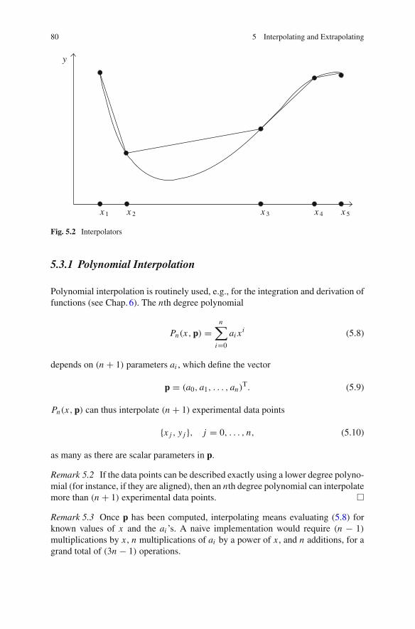
80 5 Interpolating and Extrapolating

y

x 1 x 2 x 3 x 4 x 5

Fig. 5.2 Interpolators

5.3.1 Polynomial Interpolation

Polynomial interpolation is routinely used, e.g., for the integration and derivation offunctions (see Chap. 6). The nth degree polynomial

Pn(x, p) =n∑

i=0

ai xi (5.8)

depends on (n + 1) parameters ai , which define the vector

p = (a0, a1, . . . , an)T. (5.9)

Pn(x, p) can thus interpolate (n + 1) experimental data points

{x j , y j }, j = 0, . . . , n, (5.10)

as many as there are scalar parameters in p.

Remark 5.2 If the data points can be described exactly using a lower degree polyno-mial (for instance, if they are aligned), then an nth degree polynomial can interpolatemore than (n + 1) experimental data points. �

Remark 5.3 Once p has been computed, interpolating means evaluating (5.8) forknown values of x and the ai ’s. A naive implementation would require (n − 1)

multiplications by x , n multiplications of ai by a power of x , and n additions, for agrand total of (3n − 1) operations.

5.3 Univariate Case 81

Compare with Horner’s algorithm:

⎡⎢

⎣

p0 = an

pi = pi−1x + an−i (i = 1, . . . , n)

P(x) = pn

, (5.11)

which requires only 2n operations.Note that (5.8) is not necessarily the most appropriate representation of a polyno-

mial, as the value of P(x) for any given value of x can be very sensitive to errors inthe values of the ai ’s [4]. See Remark 5.5. �

Consider polynomial interpolation for x in [−1, 1]. (Any nondegenerate interval[a, b] can be scaled to [−1, 1] by the affine transformation

xscaled = 1

b − a(2xinitial − a − b), (5.12)

so this is not restrictive.) A key point is how the x j ’s are distributed in [−1, 1]. Whenthey are regularly spaced, interpolation should only be considered practical for smallvalues of n. It may otherwise yield useless results, with spurious oscillations knownas Runge phenomenon. This can be avoided by using Chebyshev points [1, 2], forinstance Chebyshev points of the second kind, given by

x j = cosjπ

n, j → 0, 1, . . . , n. (5.13)

(Interpolation by splines (described in Sect. 5.3.2), or Kriging (described inSect. 5.4.3) could also be considered.)

Several techniques can be used to compute the interpolating polynomial. Sincethis polynomial is unique, they are mathematically equivalent (but their numericalproperties differ).

5.3.1.1 Interpolation via Lagrange’s Formula

Lagrange’s interpolation formula expresses Pn(x) as

Pn(x) =n∑

j=0

⎤

⎥⎦

k ∇= j

x − xk

x j − xk

⎞

⎠ y j . (5.14)

The evaluation of p from the data is thus bypassed. It is trivial to check that Pn(x j ) =y j since, for x = x j , all the products in (5.14) are equal to zero but the j th, whichis equal to 1. Despite its simplicity, (5.14) is seldom used in practice, because it isnumerically unstable.

A very useful reformulation is the barycentric Lagrange interpolation formula

82 5 Interpolating and Extrapolating

Pn(x) =∑n

j=0w j

x−x jy j

∑nj=0

w jx−x j

, (5.15)

where the barycentric weights satisfy

w j = 1∏k ∇= j (x j − xk)

, j → 0, 1, . . . , n. (5.16)

These weights thus depend only on the location of the evaluation points x j , not onthe values of the corresponding data y j . They can therefore be computed once andfor all for a given node configuration. The result is particularly simple for Chebyshevpoints of the second kind, as

w j = (−1) jδ j , j → 0, 1, . . . , n, (5.17)

with all δ j ’s equal to one, except for δ0 = δn = 1/2 [5].Barycentric Lagrange interpolation is so much more stable numerically than (5.14)

that it is considered as one of the best methods for polynomial interpolation [6].

5.3.1.2 Interpolation via Linear System Solving

When the interpolating polynomial is expressed as in (5.8), its parameter vector p isthe solution of the linear system

Ap = y, (5.18)

with

A =

1 x0 x20 · · · xn

0

1 x1 x21 · · · xn

1...

......

......

1 xn x2n · · · xn

n

(5.19)

and

y =

y0y1...

yn

. (5.20)

A is a Vandermonde matrix, notoriously ill-conditioned for large n.

Remark 5.4 The fact that a Vandermonde matrix is ill-conditioned does not meanthat the corresponding interpolation problem cannot be solved. With appropriatealternative formulations, it is possible to build interpolating polynomials of veryhigh degree. This is spectacularly illustrated in [2], where a sawtooth function is

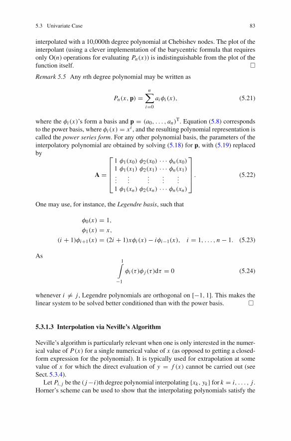
5.3 Univariate Case 83

interpolated with a 10,000th degree polynomial at Chebishev nodes. The plot of theinterpolant (using a clever implementation of the barycentric formula that requiresonly O(n) operations for evaluating Pn(x)) is indistinguishable from the plot of thefunction itself. �Remark 5.5 Any nth degree polynomial may be written as

Pn(x, p) =n∑

i=0

aiφi (x), (5.21)

where the φi (x)’s form a basis and p = (a0, . . . , an)T. Equation (5.8) correspondsto the power basis, where φi (x) = xi , and the resulting polynomial representation iscalled the power series form. For any other polynomial basis, the parameters of theinterpolatory polynomial are obtained by solving (5.18) for p, with (5.19) replacedby

A =

1 φ1(x0) φ2(x0) · · · φn(x0)

1 φ1(x1) φ2(x1) · · · φn(x1)...

......

......

1 φ1(xn) φ2(xn) · · · φn(xn)

. (5.22)

One may use, for instance, the Legendre basis, such that

φ0(x) = 1,

φ1(x) = x,

(i + 1)φi+1(x) = (2i + 1)xφi (x) − iφi−1(x), i = 1, . . . , n − 1. (5.23)

As1∫

−1

φi (τ )φ j (τ )dτ = 0 (5.24)

whenever i ∇= j , Legendre polynomials are orthogonal on [−1, 1]. This makes thelinear system to be solved better conditioned than with the power basis. �

5.3.1.3 Interpolation via Neville’s Algorithm

Neville’s algorithm is particularly relevant when one is only interested in the numer-ical value of P(x) for a single numerical value of x (as opposed to getting a closed-form expression for the polynomial). It is typically used for extrapolation at somevalue of x for which the direct evaluation of y = f (x) cannot be carried out (seeSect. 5.3.4).

Let Pi, j be the ( j −i)th degree polynomial interpolating {xk, yk} for k = i, . . . , j .Horner’s scheme can be used to show that the interpolating polynomials satisfy the

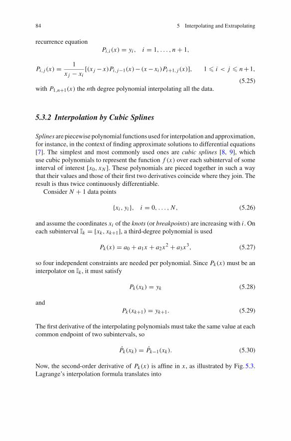
84 5 Interpolating and Extrapolating

recurrence equationPi,i (x) = yi , i = 1, . . . , n + 1,

Pi, j (x) = 1

x j − xi[(x j − x)Pi, j−1(x)− (x − xi )Pi+1, j (x)], 1 � i < j � n +1,

(5.25)with P1,n+1(x) the nth degree polynomial interpolating all the data.

5.3.2 Interpolation by Cubic Splines

Splines are piecewise polynomial functions used for interpolation and approximation,for instance, in the context of finding approximate solutions to differential equations[7]. The simplest and most commonly used ones are cubic splines [8, 9], whichuse cubic polynomials to represent the function f (x) over each subinterval of someinterval of interest [x0, xN ]. These polynomials are pieced together in such a waythat their values and those of their first two derivatives coincide where they join. Theresult is thus twice continuously differentiable.

Consider N + 1 data points

{xi , yi }, i = 0, . . . , N , (5.26)

and assume the coordinates xi of the knots (or breakpoints) are increasing with i . Oneach subinterval Ik = [xk, xk+1], a third-degree polynomial is used

Pk(x) = a0 + a1x + a2x2 + a3x3, (5.27)

so four independent constraints are needed per polynomial. Since Pk(x) must be aninterpolator on Ik , it must satisfy

Pk(xk) = yk (5.28)

andPk(xk+1) = yk+1. (5.29)

The first derivative of the interpolating polynomials must take the same value at eachcommon endpoint of two subintervals, so

Pk(xk) = Pk−1(xk). (5.30)

Now, the second-order derivative of Pk(x) is affine in x , as illustrated by Fig. 5.3.Lagrange’s interpolation formula translates into

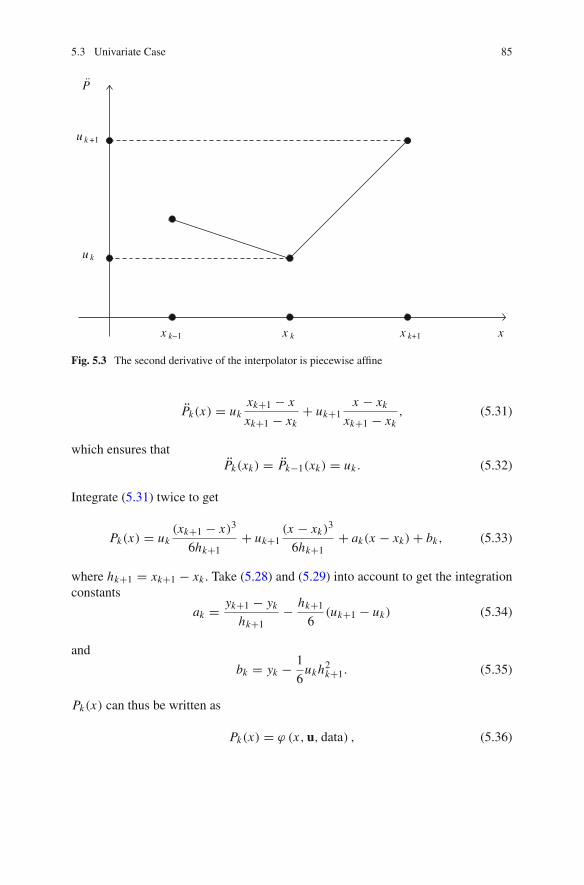
5.3 Univariate Case 85

u k +1

u k

P

xx k−1 x k x k+1

Fig. 5.3 The second derivative of the interpolator is piecewise affine

Pk(x) = ukxk+1 − x

xk+1 − xk+ uk+1

x − xk

xk+1 − xk, (5.31)

which ensures thatPk(xk) = Pk−1(xk) = uk . (5.32)

Integrate (5.31) twice to get

Pk(x) = uk(xk+1 − x)3

6hk+1+ uk+1

(x − xk)3

6hk+1+ ak(x − xk) + bk, (5.33)

where hk+1 = xk+1 − xk . Take (5.28) and (5.29) into account to get the integrationconstants

ak = yk+1 − yk

hk+1− hk+1

6(uk+1 − uk) (5.34)

and

bk = yk − 1

6ukh2

k+1. (5.35)

Pk(x) can thus be written as

Pk(x) = ϕ (x, u, data) , (5.36)

86 5 Interpolating and Extrapolating

where u is the vector comprising all the uk’s. This expression is cubic in x and affinein u.

There are (N + 1 = dim u) unknowns, and (N − 1) continuity conditions (5.30)(as there are N subintervals Ik), so two additional constraints are needed to make thesolution for u unique. In natural cubic splines, these constraints are u0 = uN = 0,which amounts to saying that the cubic spline is affine in (−⇒, x0] and [xN ,⇒).Other choices are possible; one may, for instance, fit the first derivative of f (·) at x0and xN or assume that f (·) is periodic and such that

f (x + xN − x0) ∈ f (x). (5.37)

The periodic cubic spline must then satisfy

P(r)0 (x0) = P(r)

N−1(xN ), r = 0, 1, 2. (5.38)

For any of these choices, the resulting set of linear equations can be written as

Tu = d, (5.39)

with u the vector of those ui ’s still to be estimated and T tridiagonal, which greatlyfacilitates solving (5.39) for u.

Let hmax be the largest of all the intervals hk between knots. When f (·) is suffi-ciently smooth, the interpolation error of a natural cubic spline is O(h4

max) for any xin a closed interval that tends to [x0, xN ] when hmax tends to zero [10].

5.3.3 Rational Interpolation

The rational interpolator takes the form

F(x, p) = P(x, p)

Q(x, p), (5.40)

where p is a vector of parameters to be chosen so as to enforce interpolation, andP(x, p) and Q(x, p) are polynomials.

If the power series representation of polynomials is used, then

F(x, p) =∑p

i=0 ai xi

∑qj=0 b j x j

, (5.41)

with p = (a0, . . . , ap, b0, . . . , bq)T. This implies that F(x, p) = F(x, αp) forany α ∇= 0. A constraint must therefore be put on p to make it unique for a giveninterpolator. One may impose b0 = 1, for instance. The same will hold true for anypolynomial basis in which P(x, p) and Q(x, p) may be expressed.

5.3 Univariate Case 87

The main advantage of rational interpolation over polynomial interpolation isincreased flexibility, as the class of polynomial functions is just a restricted class ofrational functions, with a constant polynomial at the denominator. Rational functionsare, for instance, much apter than polynomial functions at interpolating (or approxi-mating) functions with poles or other singularities near these singularities. Moreover,they can have horizontal or vertical asymptotes, contrary to polynomial functions.

Although there are as many equations as there are unknowns, a solution may notexist, however. Consider, for instance, the rational function

F(x, a0, a1, b1) = a0 + a1x

1 + b1x. (5.42)

It depends on three parameters and can thus, in principle, be used to interpolate f (x)

at three values of x . Assume that f (x0) = f (x1) ∇= f (x2). Then

a0 + a1x0

1 + b1x0= a0 + a1x1

1 + b1x1. (5.43)

This implies that a1 = a0b1 and the rational function simplifies into

F(x, a0, a1, b1) = a0 = f (x0) = f (x1). (5.44)

It is therefore unable to fit f (x2). This pole-zero cancellation can be eliminated bymaking f (x0) slightly different from f (x1), thus replacing interpolation by approx-imation, and cancellation by near cancellation. Near cancellation is rather commonwhen interpolating actual data with rational functions. It makes the problem ill-posed(the value of the coefficients of the interpolator become very sensitive to the data).

While the rational interpolator F(x, p) is linear in the parameters ai of its numer-ator, it is nonlinear in the parameters b j of its denominator. In general, the constraintsenforcing interpolation

F(xi , p) = f (xi ), i = 1, . . . , n, (5.45)

thus define a set of nonlinear equations in p, the solution of which seems to requiretools such as those described in Chap. 7. This system, however, can be transformedinto a linear one by multiplying the i th equation in (5.45) by Q(xi , p) (i = 1, . . . , n)

to get the mathematically equivalent system of equations

Q(xi , p) f (xi ) = P(xi , p), i = 1, . . . , n, (5.46)

which is linear in p. Recall that a constraint should be imposed on p to make thesolution generically unique, and that pole-zero cancellation or near cancellation mayhave to be taken care of, often by approximating the data rather than interpolatingthem.

88 5 Interpolating and Extrapolating

5.3.4 Richardson’s Extrapolation

Let R(h) be the approximate value provided by some numerical method for somemathematical result r , with h > 0 the step-size of this method. Assume that

r = limh→0

R(h), (5.47)

but that it is impossible in practice to make h tend to zero, as in the two followingexamples.

Example 5.4 Evaluation of derivativesOne possible finite-difference approximation of the first-order derivative of a

function f (·) is

f (x) √ 1

h[ f (x + h) − f (x)] (5.48)

(see Chap. 6). Mathematically, the smaller h is the better the approximation becomes,but making h too small is a recipe for disaster in floating-point computations, as itentails computing the difference of numbers that are too close to one another. �

Example 5.5 Evaluation of integralsThe rectangle method can be used to approximate the definite integral of a function

f (·) asb∫

a

f (τ )dτ √∑

i

h f (a + ih). (5.49)

Mathematically, the smaller h is the better the approximation becomes, but when his too small the approximation requires too much computer time to be evaluated. �

Because h cannot tend to zero, using R(h) instead of r introduces a method error,and extrapolation may be used to improve accuracy on the evaluation of r . Assumethat

r = R(h) + O(hn), (5.50)

where the order n of the method error is known. Richardson’s extrapolation principletakes advantage of this knowledge to increase accuracy by combining results obtainedat various step-sizes. Equation (5.50) can be rewritten as

r = R(h) + cnhn + cn+1hn+1 + · · · (5.51)

and, with a step-size divided by two,

r = R(h

2) + cn

(h

2

)n

+ cn+1

(h

2

)n+1

+ · · · (5.52)

5.3 Univariate Case 89

To eliminate the nth order term, subtract (5.51) from 2n times (5.52) to get

(2n − 1

)r = 2n R

(h

2

)− R(h) + O(hm), (5.53)

with m > n, or equivalently

r = 2n R( h

2

) − R(h)

2n − 1+ O(hm). (5.54)

Two evaluations of R have thus made it possible to gain at least one order of approx-imation. The idea can be pushed further by evaluating R(hi ) for several values ofhi obtained by successive divisions by two of some initial step-size h0. The value ath = 0 of the polynomial P(h) extrapolating the resulting data (hi , R(hi )) may thenbe computed with Neville’s algorithm (see Sect. 5.3.1.3). In the context of the evalua-tion of definite integrals, the result is Romberg’s method, see Sect. 6.2.2. Richardson’sextrapolation is also used, for instance, in numerical differentiation (see Sect. 6.4.3),as well as for the integration of ordinary differential equations (see the Bulirsch-Stoermethod in Sect. 12.2.4.6).

Instead of increasing accuracy, one may use similar ideas to adapt the step-size hin order to keep an estimate of the method error acceptable (see Sect. 12.2.4).

5.4 Multivariate Case

Assume now that there are several input variables (also called input factors), whichform a vector x, and several output variables, which form a vector y. The problemis then MIMO (for multi-input multi-output). To simplify presentation, we consideronly one output denoted by y, so the problem is MISO (for multi-input single output).MIMO problems can always be split into as many MISO problems as there areoutputs, although this is not necessarily a good idea.

5.4.1 Polynomial Interpolation

In multivariate polynomial interpolation, each input variable appears as an unknownof the polynomial. If, for instance, there are two input variables x1 and x2 and thetotal degree of the polynomial is two, then it can be written as

P(x, p) = a0 + a1x1 + a2x2 + a3x21 + a4x1x2 + a5x2

2 . (5.55)

This polynomial is still linear in the vector of its unknown coefficients

90 5 Interpolating and Extrapolating

p = (a0, a1, . . . , a5)T, (5.56)

and this holds true whatever the degree of the polynomial and the number of inputvariables. The values of these coefficients can therefore always be computed bysolving a set of linear equations enforcing interpolation, provided there are enoughof them. The choice of the structure of the polynomial (of which monomials toinclude) is far from trivial, however.

5.4.2 Spline Interpolation

The presentation of cubic splines in the univariate case suggests that multivariatesplines might be a complicated matter. Cubic splines can actually be recast as aspecial case of Kriging [11, 12], and the treatment of Kriging in the multivariatecase is rather simple, at least in principle.

5.4.3 Kriging

The name Kriging is a tribute to the seminal work of D.G. Krige on the Witwatersrandgold deposits in South Africa, circa 1950 [13]. The technique was developed andpopularized by G. Matheron, from the Centre de géostatistique of the École desmines de Paris, one of the founders of geostatistics where it plays a central role [12,14, 15]. Initially applied on two- and three-dimensional problems where the inputfactors corresponded to space variables (as in mining), it extends directly to problemswith a much larger number of input factors (as is common in industrial statistics).

We describe here, with no mathematical justification for the time being, how thesimplest version of Kriging can be used for multidimensional interpolation. Moreprecise statements, including a derivation of the equations, are in Example 9.2.

Let y(x) be the scalar output value to be predicted based on the value taken bythe input vector x. Assume that a series of experiments (which may be computerexperiments or actual measurements in the physical world) has provided the outputvalues

yi = f (xi ), i = 1, . . . , N , (5.57)

for N numerical values xi of the input vector, and denote the vector of these outputvalues by y. Note that the meaning of y here differs from that in (5.1). The Krigingprediction y(x) of the value taken by f (x) for x ∇→ {xi , i = 1, . . . , N } is linear in y,and the weights of the linear combination depend on the value of x. Thus,

y(x) = cT(x)y. (5.58)

5.4 Multivariate Case 91

It seems natural to assume that the closer x is to xi , the more f (x) resembles f (xi ).This leads to defining a correlation function r(x, xi ) between f (x) and f (xi ) suchthat

r(xi , xi ) = 1 (5.59)

and that r(x, xi ) decreases toward zero when the distance between x et xi increases.This correlation function often depends on a vector p of parameters to be tuned fromthe available data. It will then be denoted by r(x, xi , p).

Example 5.6 Correlation function for KrigingA frequently employed parametrized correlation function is

r(x, xi , p) =dim x⎦

j=1

exp(−p j |x j − xij |2). (5.60)

The range parameters p j > 0 specify how quickly the influence of the measurementyi decreases when the distance to xi increases. If p is too large, then the influence ofthe data quickly vanishes and y(x) tends to zero whenever x is not in the immediatevicinity of some xi . �

Assume, for the sake of simplicity, that the value of p has been chosen before-hand, so it no longer appears in the equations. (Statistical methods are available forestimating p from the data, see Remark 9.5.)

The Kriging prediction is Gaussian, and thus entirely characterized (for any givenvalue of the input vector x) by its mean y(x) and variance σ 2(x). The mean of theprediction is

y(x) = rT(x)R−1y, (5.61)

where

R =

r(x1, x1) r(x1, x2) · · · r(x1, xN )

r(x2, x1) r(x2, x2) · · · r(x2, xN )...

.... . .

...

r(xN , x1) r(xN , x2) · · · r(xN , xN )

(5.62)

andrT(x) = [

r(x, x1) r(x, x2) · · · r(x, xN )]. (5.63)

The variance of the prediction is

σ 2(x) = σ 2y

[1 − rT(x)R−1r(x)

], (5.64)

where σ 2y is a proportionality constant, which may also be estimated from the data,

see Remark 9.5.

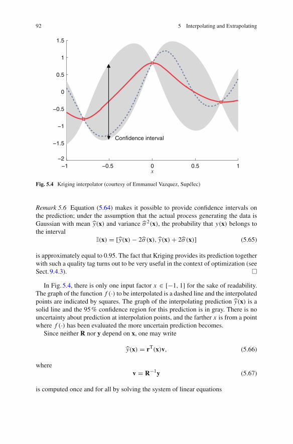
92 5 Interpolating and Extrapolating

−1 −0.5 0 0.5 1−2

−1.5

−1

−0.5

0

0.5

1

1.5

x

Confidence interval

Fig. 5.4 Kriging interpolator (courtesy of Emmanuel Vazquez, Supélec)

Remark 5.6 Equation (5.64) makes it possible to provide confidence intervals onthe prediction; under the assumption that the actual process generating the data isGaussian with mean y(x) and variance σ 2(x), the probability that y(x) belongs tothe interval

I(x) = [y(x) − 2σ (x), y(x) + 2σ (x)] (5.65)

is approximately equal to 0.95. The fact that Kriging provides its prediction togetherwith such a quality tag turns out to be very useful in the context of optimization (seeSect. 9.4.3). �

In Fig. 5.4, there is only one input factor x → [−1, 1] for the sake of readability.The graph of the function f (·) to be interpolated is a dashed line and the interpolatedpoints are indicated by squares. The graph of the interpolating prediction y(x) is asolid line and the 95 % confidence region for this prediction is in gray. There is nouncertainty about prediction at interpolation points, and the farther x is from a pointwhere f (·) has been evaluated the more uncertain prediction becomes.

Since neither R nor y depend on x, one may write

y(x) = rT(x)v, (5.66)

wherev = R−1y (5.67)

is computed once and for all by solving the system of linear equations

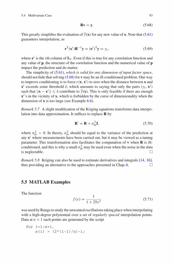
5.4 Multivariate Case 93

Rv = y. (5.68)

This greatly simplifies the evaluation of y(x) for any new value of x. Note that (5.61)guarantees interpolation, as

rT(xi )R−1y = (ei )Ty = yi , (5.69)

where ei is the i th column of IN . Even if this is true for any correlation function andany value of p, the structure of the correlation function and the numerical value of pimpact the prediction and do matter.

The simplicity of (5.61), which is valid for any dimension of input factor space,should not hide that solving (5.68) for v may be an ill-conditioned problem. One wayto improve conditioning is to force r(x, xi ) to zero when the distance between x andxi exceeds some threshold δ, which amounts to saying that only the pairs (yi , xi )

such that ||x − xi || � δ contribute to y(x). This is only feasible if there are enoughxi ’s in the vicinity of x, which is forbidden by the curse of dimensionality when thedimension of x is too large (see Example 8.6).

Remark 5.7 A slight modification of the Kriging equations transforms data interpo-lation into data approximation. It suffices to replace R by

R⊂ = R + σ 2mI, (5.70)

where σ 2m > 0. In theory, σ 2

m should be equal to the variance of the prediction atany xi where measurements have been carried out, but it may be viewed as a tuningparameter. This transformation also facilitates the computation of v when R is ill-conditioned, and this is why a small σ 2

m may be used even when the noise in the datais neglectable. �

Remark 5.8 Kriging can also be used to estimate derivatives and integrals [14, 16],thus providing an alternative to the approaches presented in Chap. 6. �

5.5 MATLAB Examples

The function

f (x) = 1

1 + 25x2 (5.71)

was used by Runge to study the unwanted oscillations taking place when interpolatingwith a high-degree polynomial over a set of regularly spaced interpolation points.Data at n + 1 such points are generated by the script

for i=1:n+1,x(i) = (2*(i-1)/n)-1;

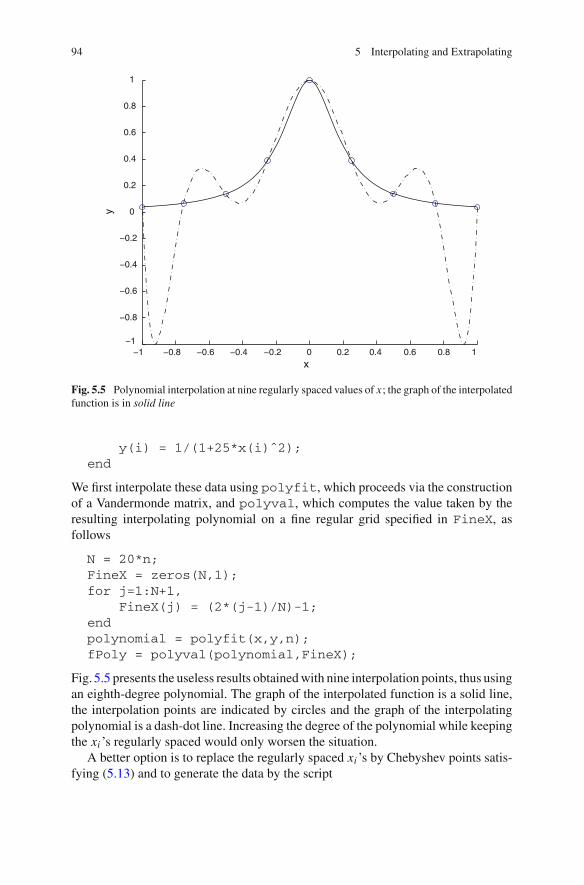
94 5 Interpolating and Extrapolating

−1 −0.8 −0.6 −0.4 −0.2 0 0.2 0.4 0.6 0.8 1−1

−0.8

−0.6

−0.4

−0.2

0

0.2

0.4

0.6

0.8

1

x

y

Fig. 5.5 Polynomial interpolation at nine regularly spaced values of x ; the graph of the interpolatedfunction is in solid line

y(i) = 1/(1+25*x(i)ˆ2);end

We first interpolate these data using polyfit, which proceeds via the constructionof a Vandermonde matrix, and polyval, which computes the value taken by theresulting interpolating polynomial on a fine regular grid specified in FineX, asfollows

N = 20*n;FineX = zeros(N,1);for j=1:N+1,

FineX(j) = (2*(j-1)/N)-1;endpolynomial = polyfit(x,y,n);fPoly = polyval(polynomial,FineX);

Fig. 5.5 presents the useless results obtained with nine interpolation points, thus usingan eighth-degree polynomial. The graph of the interpolated function is a solid line,the interpolation points are indicated by circles and the graph of the interpolatingpolynomial is a dash-dot line. Increasing the degree of the polynomial while keepingthe xi ’s regularly spaced would only worsen the situation.

A better option is to replace the regularly spaced xi ’s by Chebyshev points satis-fying (5.13) and to generate the data by the script

5.5 MATLAB Examples 95

−1 −0.8 −0.6 −0.4 −0.2 0 0.2 0.4 0.6 0.8 10

0.1

0.2

0.3

0.4

0.5

0.6

0.7

0.8

0.9

1

x

y

Fig. 5.6 Polynomial interpolation at 21 Chebyshev values of x ; the graph of the interpolatedfunction is in solid line

for i=1:n+1,x(i) = cos((i-1)*pi/n);y(i) = 1/(1+25*x(i)ˆ2);

end

The results with nine interpolation points still show some oscillations, but we cannow safely increase the order of the polynomial to improve the situation. With 21interpolation points, we get the results of Fig. 5.6.

An alternative option is to use cubic splines. This can be carried out by using thefunctions spline, which computes the piecewise polynomial, and ppval, whichevaluates this piecewise polynomial at points to be specified. One may thus write

PieceWisePol = spline(x,y);fCubicSpline = ppval(PieceWisePol,FineX);

With nine regularly spaced xi ’s, the results are then as presented in Fig. 5.7.

5.6 In Summary

• Prefer interpolation to extrapolation, whenever possible.• Interpolation may not be the right answer to an approximation problem; there is

no point in interpolating noisy or uncertain data.

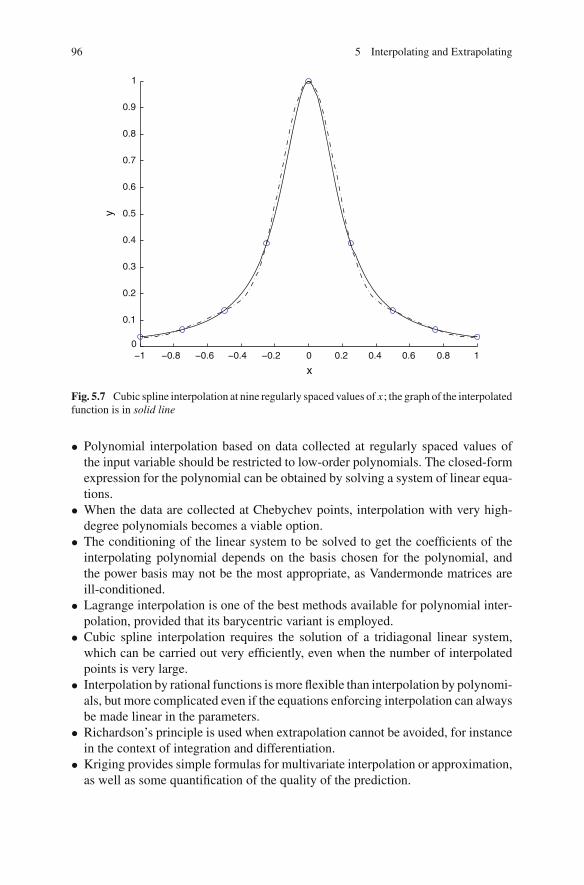
96 5 Interpolating and Extrapolating

−1 −0.8 −0.6 −0.4 −0.2 0 0.2 0.4 0.6 0.8 10

0.1

0.2

0.3

0.4

0.5

0.6

0.7

0.8

0.9

1

x

y

Fig. 5.7 Cubic spline interpolation at nine regularly spaced values of x ; the graph of the interpolatedfunction is in solid line

• Polynomial interpolation based on data collected at regularly spaced values ofthe input variable should be restricted to low-order polynomials. The closed-formexpression for the polynomial can be obtained by solving a system of linear equa-tions.

• When the data are collected at Chebychev points, interpolation with very high-degree polynomials becomes a viable option.

• The conditioning of the linear system to be solved to get the coefficients of theinterpolating polynomial depends on the basis chosen for the polynomial, andthe power basis may not be the most appropriate, as Vandermonde matrices areill-conditioned.

• Lagrange interpolation is one of the best methods available for polynomial inter-polation, provided that its barycentric variant is employed.

• Cubic spline interpolation requires the solution of a tridiagonal linear system,which can be carried out very efficiently, even when the number of interpolatedpoints is very large.

• Interpolation by rational functions is more flexible than interpolation by polynomi-als, but more complicated even if the equations enforcing interpolation can alwaysbe made linear in the parameters.

• Richardson’s principle is used when extrapolation cannot be avoided, for instancein the context of integration and differentiation.

• Kriging provides simple formulas for multivariate interpolation or approximation,as well as some quantification of the quality of the prediction.

References 97

References

1. Trefethen, L.: Approximation Theory and Approximation Practice. SIAM, Philadelphia (2013)2. Trefethen, L.: Six myths of polynomial interpolation and quadrature. Math. Today 47, 184–188

(2011)3. Sacks, J., Welch, W., Mitchell, T., Wynn, H.: Design and analysis of computer experiments

(with discussion). Stat. Sci. 4(4), 409–435 (1989)4. Farouki, R.: The Bernstein polynomial basis: a centennial retrospective. Comput. Aided Geom.

Des. 29, 379–419 (2012)5. Berrut, J.P., Trefethen, L.: Barycentric Lagrange interpolation. SIAM Rev. 46(3), 501–517

(2004)6. Higham, N.: The numerical stability of barycentric Lagrange interpolation. IMA J. Numer.

Anal. 24(4), 547–556 (2004)7. de Boor, C.: Package for calculating with B-splines. SIAM J. Numer. Anal. 14(3), 441–472

(1977)8. Stoer, J., Bulirsch, R.: Introduction to Numerical Analysis. Springer, New York (1980)9. de Boor, C.: A Practical Guide to Splines, revised edn. Springer, New York (2001)

10. Kershaw, D.: A note on the convergence of interpolatory cubic splines. SIAM J. Numer. Anal.8(1), 67–74 (1971)

11. Wahba, G.: Spline Models for Observational Data. SIAM, Philadelphia (1990)12. Cressie, N.: Statistics for Spatial Data. Wiley, New York (1993)13. Krige, D.: A statistical approach to some basic mine valuation problems on the Witwatersrand.

J. Chem. Metall. Min. Soc. 52, 119–139 (1951)14. Chilès, J.P., Delfiner, P.: Geostatistics. Wiley, New York (1999)15. Wackernagel, H.: Multivariate Geostatistics, 3rd edn. Springer, Berlin (2003)16. Vazquez, E., Walter, E.: Estimating derivatives and integrals with Kriging. In: Proceedings

of 44th IEEE Conference on Decision and Control (CDC) and European Control Conference(ECC), pp. 8156–8161. Seville, Spain (2005)

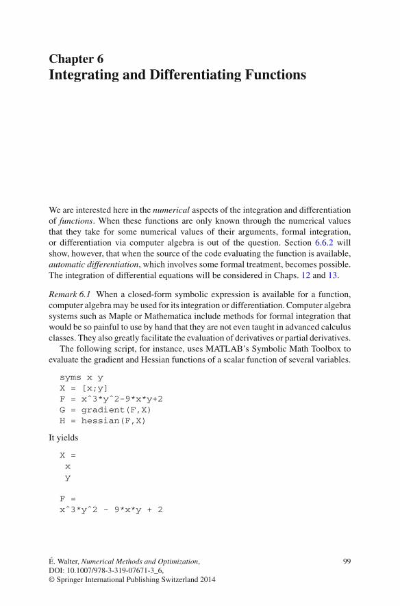
Chapter 6Integrating and Differentiating Functions

We are interested here in the numerical aspects of the integration and differentiationof functions. When these functions are only known through the numerical valuesthat they take for some numerical values of their arguments, formal integration,or differentiation via computer algebra is out of the question. Section 6.6.2 willshow, however, that when the source of the code evaluating the function is available,automatic differentiation, which involves some formal treatment, becomes possible.The integration of differential equations will be considered in Chaps. 12 and 13.

Remark 6.1 When a closed-form symbolic expression is available for a function,computer algebra may be used for its integration or differentiation. Computer algebrasystems such as Maple or Mathematica include methods for formal integration thatwould be so painful to use by hand that they are not even taught in advanced calculusclasses. They also greatly facilitate the evaluation of derivatives or partial derivatives.

The following script, for instance, uses MATLAB’s Symbolic Math Toolbox toevaluate the gradient and Hessian functions of a scalar function of several variables.

syms x yX = [x;y]F = xˆ3*yˆ2-9*x*y+2G = gradient(F,X)H = hessian(F,X)

It yields

X =xy

F =xˆ3*yˆ2 - 9*x*y + 2

É. Walter, Numerical Methods and Optimization, 99DOI: 10.1007/978-3-319-07671-3_6,© Springer International Publishing Switzerland 2014

100 6 Integrating and Differentiating Functions

G =3*xˆ2*yˆ2 - 9*y

2*y*xˆ3 - 9*x

H =[ 6*x*yˆ2, 6*y*xˆ2 - 9][ 6*y*xˆ2 - 9, 2*xˆ3]

For vector functions of several variables, Jacobian matrices may be similarly gener-ated, see Remark 7.10.

It is not assumed here that such closed-form expressions of the functions to beintegrated or differentiated are available. �

6.1 Examples

Example 6.1 Inertial navigationInertial navigation systems are used, e.g., in aircraft and submarines. They include

accelerometers that measure acceleration along three independent axes (say, longi-tude, latitude, and altitude). Integrating these accelerations once, one can evaluatethe three components of speed, and a second integration leads to the three compo-nents of position, provided the initial conditions are known. Cheap accelerometers,as made possible by micro electromechanical systems (MEMS), have found theirway into smartphones, videogame consoles and other personal electronic devices.See Sect. 16.23. �

Example 6.2 Power estimationThe power P consumed by an electrical appliance (in W) is

P = 1

T

T∫

0

u(τ )i(τ )dτ, (6.1)

where the electric tension u delivered to the appliance (in V) is sinusoidal with periodT , and where (possibly after some transient) the current i through the appliance (in A)is also periodic with period T , but not necessarily sinusoidal. To estimate the valueof P from measurements of u(tk) and i(tk) at some instants of time tk √ [0, T ],k = 1, . . . , N , one has to evaluate an integral. �

Example 6.3 Speed estimationComputing the speed of a mobile from measurements of its position boils down

to differentiating a signal, the value of which is only known at discrete instants oftime. (When a model of the dynamical behavior of the mobile is available, it may betaken into account via the use of a Kalman filter [1, 2], not considered here.) �

6.1 Examples 101

Example 6.4 Integration of differential equationsThe finite-difference method for integrating ordinary or partial differential

equations heavily relies on formulas for numerical differentiation. See Chaps. 12and 13. �

6.2 Integrating Univariate Functions

Consider the definite integral

I =b∫

a

f (x)dx, (6.2)

where the lower limit a and upper limit b have known numerical values and where theintegrand f (·), a real function assumed to be integrable, can be evaluated numericallyat any x in [a, b]. Evaluating I is often called quadrature, a reminder of the methodapproximating areas by unions of small squares.

Since, for any c √ [a, b], for instance its middle,

b∫

a

f (x)dx =c∫

a

f (x)dx +b∫

c

f (x)dx, (6.3)

the computation of I may recursively be split into subtasks whenever this is ex-pected to lead to better accuracy, in a divide-and-conquer approach. This is adaptivequadrature, which makes it possible to adapt to local properties of the integrand f (·)by putting more evaluations where f (·) varies quickly.

The decision about whether to bisect [a, b] is usually taken based on comparingthe numerical results I+ and I− of the evaluation of I by two numerical integrationmethods, with I+ expected to be more accurate than I−. If

|I+ − I−||I+| < δ, (6.4)

where δ is some prescribed relative error tolerance, then the result I+ provided bythe better method is kept, else [a, b] may be bisected and the same procedure appliedto the two resulting subintervals. To avoid endless bisections, a limit is set on thenumber of recursion levels and no bisection is carried out on subintervals such thattheir relative contribution to I is deemed too small. See [3] for a comparison ofstrategies for adaptive quadrature and evidence of the fact that none of them willgive accurate answers for all integrable functions.

The interval [a, b] considered in what follows may be one of the subintervalsresulting from such a divide-and-conquer approach.

102 6 Integrating and Differentiating Functions

6.2.1 Newton–Cotes Methods

In Newton-Cotes methods, f (·) is evaluated at (N + 1) regularly spaced points xi ,i = 0, . . . , N , such that x0 = a and xN = b, so

xi = a + ih, i = 0, . . . , N , (6.5)

with

h = b − a

N. (6.6)

The interval [a, b] is partitioned into subintervals with equal width kh, so k mustdivide N . Each subinterval contains (k+1) evaluation points, which makes it possibleto replace f (·) on this subinterval by a kth degree interpolating polynomial. Thevalue of the definite integral I is then approximated by the sum of the integrals ofthe interpolating polynomials over the subintervals on which they interpolate f (·).Remark 6.2 The initial problem has thus been replaced by an approximate one thatcan be solved exactly (at least from a mathematical point of view). �

Remark 6.3 Spacing the evaluation points regularly may not be such a good idea,see Sects. 6.2.3 and 6.2.4. �

The integral of the interpolating polynomial over the subinterval [x0, xk] can thenbe written as

ISI(k) = hk⎡

j=0

c j f (x j ), (6.7)

where the coefficients c j depend only on the order k of the polynomial, and the sameformula applies for any one of the other subintervals, after a suitable incrementationof the indices.

In what follows, NC(k) denotes the Newton-Cotes method based on an interpo-lating polynomial with order k, and f (x j ) is denoted by f j . Because the x j ’s areequispaced, the order k must be small. The local method error committed by NC(k)over [x0, xk] is

eNC(k) =xk∫

x0

f (x)dx − ISI(k), (6.8)

and the global method error over [a, b], denoted by ENC(k), is obtained by summingthe local method errors committed over all the subintervals.

6.2 Integrating Univariate Functions 103

Proofs of the results concerning the values of eNC(k) and ENC(k) presented belowcan be found in [4]. In these results, f (·) is of course assumed to be differentiableup to the order required.

6.2.1.1 NC(1): Trapezoidal Rule

A first-order interpolating polynomial requires two evaluation points per subinterval(one at each endpoint). Interpolation is then piecewise affine, and the integral of f (·)over [x0, x1] is given by the trapezoidal rule

ISI = h

2( f0 + f1) = b − a

2N( f0 + f1). (6.9)

All endpoints are used twice when evaluating I , except for x0 and xN , so

I ∇ b − a

N

⎢f0 + fN

2+

N−1⎡

i=1

fi

⎣. (6.10)

The local method error satisfies

eNC(1) = − 1

12f (η)h3, (6.11)

for some η √ [x0, x1], and the global method error is such that

ENC(1) = −b − a

12f (ζ )h2, (6.12)

for some ζ √ [a, b]. The global method error on I is thus O(h2). If f (·) is apolynomial of degree at most one, then f (·) → 0 and there is no method error,which should come as no surprise.

Remark 6.4 The trapezoidal rule can also be used with irregularly spaced xi ’s, as

I ∇ 1

2

N−1⎡

i=0

(xi+1 − xi ) · ( fi+1 + fi ). (6.13)

�

6.2.1.2 NC(2): Simpson’s 1/3 Rule

A second-order interpolating polynomial requires three evaluation points persubinterval. Interpolation is then piecewise parabolic, and

104 6 Integrating and Differentiating Functions

ISI = h

3( f0 + 4 f1 + f2). (6.14)

The name 1/3 comes from the leading coefficient in (6.14). It can be shown that

eNC(2) = − 1

90f (4)(η)h5, (6.15)

for some η √ [x0, x2], and

ENC(2) = −b − a

180f (4)(ζ )h4, (6.16)

for some ζ √ [a, b]. The global method error on I with NC(2) is thus O(h4), muchbetter than with NC(1). Because of a lucky cancelation, there is no method error iff (·) is a polynomial of degree at most three, and not just two as one might expect.

6.2.1.3 NC(3): Simpson’s 3/8 Rule

A third-order interpolating polynomial leads to

ISI = 3

8h( f0 + 3 f1 + 3 f2 + f3). (6.17)

The name 3/8 comes from the leading coefficient in (6.17). It can be shown that

eNC(3) = − 3

80f (4)(η)h5, (6.18)

for some η √ [x0, x3], and

ENC(3) = −b − a

80f (4)(ζ )h4, (6.19)

for some ζ √ [a, b]. The global method error on I with NC(3) is thus O(h4), justas with NC(2), and nothing seems to have been gained by increasing the order ofthe interpolating polynomial. As with NC(2), there is no method error if f (·) is apolynomial of degree at most three, but for NC(3) this is not surprising.

6.2.1.4 NC(4): Boole’s Rule

Boole’s rule is sometimes called Bode’s rule, apparently as the result of a typo in anearly reference. A fourth-order interpolating polynomial leads to

6.2 Integrating Univariate Functions 105

ISI = 2

45h(7 f0 + 32 f1 + 12 f2 + 32 f3 + 7 f4). (6.20)

It can be shown that

eNC(4) = − 8

945f (6)(η)h7, (6.21)

for some η √ [x0, x4], and

ENC(4) = −2(b − a)

945f (6)(ζ )h6, (6.22)

for some ζ √ [a, b]. The global method error on I with NC(4) is thus O(h6). Againbecause of a lucky cancelation, there is no method error if f (·) is a polynomial ofdegree at most five.

Remark 6.5 A cursory look at the previous formulas may suggest that

ENC(k) = b − a

kheNC(k), (6.23)

which seems natural since the number of subintervals is (b − a)/kh. Note, however,that ζ in the expression for ENC(k) is not the same as η in that for eNC(k). �

6.2.1.5 Tuning the Step-Size of an NC Method

The step-size h should be small enough for accuracy to be acceptable, yet not toosmall as this would unnecessarily increase the number of operations. The followingprocedure may be used to assess method error and keep it at an acceptable level bytuning the step-size.

Let ⎤I (h, m) be the value obtained for I when the step-size is h and the methoderror is O(hm). Then,

I = ⎤I (h, m) + O(hm). (6.24)

In other words,I = ⎤I (h, m) + c1hm + c2hm+1 + · · · (6.25)

When the step-size is halved,

I = ⎤I⎥

h

2, m

⎦+ c1

⎥h

2

⎦m

+ c2

⎥h

2

⎦m+1

+ · · · (6.26)

Instead of combining (6.25) and (6.26) to eliminate the first method-error term, asRichardson’s extrapolation would suggest, we use the difference between ⎤I

⎞ h2 , m

⎠

and ⎤I (h, m) to get a rough estimate of the global method error for the smaller step-size. Subtract (6.26) from (6.25) to get

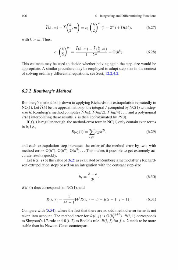
106 6 Integrating and Differentiating Functions

⎤I (h, m) − ⎤I⎥

h

2, m

⎦= c1

⎥h

2

⎦m

(1 − 2m) + O(hk), (6.27)

with k > m. Thus,

c1

⎥h

2

⎦m

=⎤I (h, m) − ⎤I

⎞ h2 , m

⎠

1 − 2m+ O(hk). (6.28)

This estimate may be used to decide whether halving again the step-size would beappropriate. A similar procedure may be employed to adapt step-size in the contextof solving ordinary differential equations, see Sect. 12.2.4.2.

6.2.2 Romberg’s Method

Romberg’s method boils down to applying Richardson’s extrapolation repeatedly toNC(1). Let ⎤I (h) be the approximation of the integral I computed by NC(1) with step-size h. Romberg’s method computes ⎤I (h0), ⎤I (h0/2), ⎤I (h0/4) . . . , and a polynomialP(h) interpolating these results. I is then approximated by P(0).

If f (·) is regular enough, the method-error term in NC(1) only contain even termsin h, i.e.,

ENC(1) =⎡

i�1

c2i h2i , (6.29)

and each extrapolation step increases the order of the method error by two, withmethod errors O(h4), O(h6), O(h8) . . . This makes it possible to get extremely ac-curate results quickly.

Let R(i, j)be the value of (6.2) as evaluated by Romberg’s method after j Richard-son extrapolation steps based on an integration with the constant step-size

hi = b − a

2i. (6.30)

R(i, 0) thus corresponds to NC(1), and

R(i, j) = 1

4 j − 1[4 j R(i, j − 1) − R(i − 1, j − 1)]. (6.31)

Compare with (5.54), where the fact that there are no odd method error terms is nottaken into account. The method error for R(i, j) is O(h2 j+2

i ). R(i, 1) correspondsto Simpson’s 1/3 rule and R(i, 2) to Boole’s rule. R(i, j) for j > 2 tends to be morestable than its Newton-Cotes counterpart.

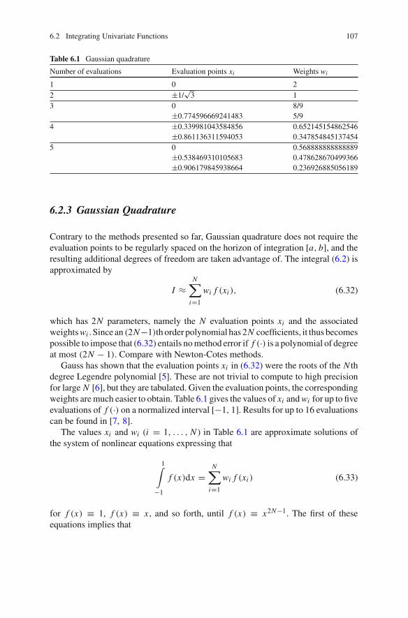
6.2 Integrating Univariate Functions 107

Table 6.1 Gaussian quadrature

Number of evaluations Evaluation points xi Weights wi

1 0 22 ±1/

⇒3 1

3 0 8/9±0.774596669241483 5/9

4 ±0.339981043584856 0.652145154862546±0.861136311594053 0.347854845137454

5 0 0.568888888888889±0.538469310105683 0.478628670499366±0.906179845938664 0.236926885056189

6.2.3 Gaussian Quadrature

Contrary to the methods presented so far, Gaussian quadrature does not require theevaluation points to be regularly spaced on the horizon of integration [a, b], and theresulting additional degrees of freedom are taken advantage of. The integral (6.2) isapproximated by

I ∇N⎡

i=1

wi f (xi ), (6.32)

which has 2N parameters, namely the N evaluation points xi and the associatedweights wi . Since an (2N−1)th order polynomial has 2N coefficients, it thus becomespossible to impose that (6.32) entails no method error if f (·) is a polynomial of degreeat most (2N − 1). Compare with Newton-Cotes methods.

Gauss has shown that the evaluation points xi in (6.32) were the roots of the N thdegree Legendre polynomial [5]. These are not trivial to compute to high precisionfor large N [6], but they are tabulated. Given the evaluation points, the correspondingweights are much easier to obtain. Table 6.1 gives the values of xi and wi for up to fiveevaluations of f (·) on a normalized interval [−1, 1]. Results for up to 16 evaluationscan be found in [7, 8].

The values xi and wi (i = 1, . . . , N ) in Table 6.1 are approximate solutions ofthe system of nonlinear equations expressing that

1∫

−1

f (x)dx =N⎡

i=1

wi f (xi ) (6.33)

for f (x) → 1, f (x) → x , and so forth, until f (x) → x2N−1. The first of theseequations implies that

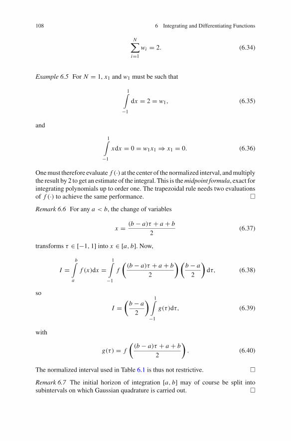
108 6 Integrating and Differentiating Functions

N⎡

i=1

wi = 2. (6.34)

Example 6.5 For N = 1, x1 and w1 must be such that

1∫

−1

dx = 2 = w1, (6.35)

and

1∫

−1

xdx = 0 = w1x1 ∈ x1 = 0. (6.36)

One must therefore evaluate f (·) at the center of the normalized interval, and multiplythe result by 2 to get an estimate of the integral. This is the midpoint formula, exact forintegrating polynomials up to order one. The trapezoidal rule needs two evaluationsof f (·) to achieve the same performance. �

Remark 6.6 For any a < b, the change of variables

x = (b − a)τ + a + b

2(6.37)

transforms τ √ [−1, 1] into x √ [a, b]. Now,

I =b∫

a

f (x)dx =1∫

−1

f

⎥(b − a)τ + a + b

2

⎦ ⎥b − a

2

⎦dτ, (6.38)

so

I =⎥

b − a

2

⎦ 1∫

−1

g(τ )dτ, (6.39)

with

g(τ ) = f

⎥(b − a)τ + a + b

2

⎦. (6.40)

The normalized interval used in Table 6.1 is thus not restrictive. �

Remark 6.7 The initial horizon of integration [a, b] may of course be split intosubintervals on which Gaussian quadrature is carried out. �

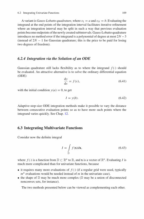
6.2 Integrating Univariate Functions 109

A variant is Gauss-Lobatto quadrature, where x1 = a and xN = b. Evaluating theintegrand at the end points of the integration interval facilitates iterative refinementwhere an integration interval may be split in such a way that previous evaluationpoints become endpoints of the newly created subintervals. Gauss-Lobatto quadratureintroduces no method error if the integrand is a polynomial of degree at most 2N −3(instead of 2N − 1 for Gaussian quadrature; this is the price to be paid for losingtwo degrees of freedom).

6.2.4 Integration via the Solution of an ODE

Gaussian quadrature still lacks flexibility as to where the integrand f (·) shouldbe evaluated. An attractive alternative is to solve the ordinary differential equation(ODE)

dy

dx= f (x), (6.41)

with the initial condition y(a) = 0, to get

I = y(b). (6.42)

Adaptive-step-size ODE integration methods make it possible to vary the distancebetween consecutive evaluation points so as to have more such points where theintegrand varies quickly. See Chap. 12.

6.3 Integrating Multivariate Functions

Consider now the definite integral

I =∫

D

f (x)dx, (6.43)

where f (·) is a function from D ⊂ Rn to R, and x is a vector of Rn . Evaluating I is

much more complicated than for univariate functions, because

• it requires many more evaluations of f (·) (if a regular grid were used, typicallymn evaluations would be needed instead of m in the univariate case),

• the shape of D may be much more complex (D may be a union of disconnectednonconvex sets, for instance).

The two methods presented below can be viewed as complementing each other.

110 6 Integrating and Differentiating Functions

integrationexternal

internal integration

y

x

Fig. 6.1 Nested 1D integrations

6.3.1 Nested One-Dimensional Integrations

Assume, for the sake of simplicity, that n = 2 and D is as indicated on Fig. 6.1. Thedefinite integral I can then be expressed as

I =y2∫

y1

x2(y)∫

x1(y)

f (x, y)dxdy, (6.44)

so one may perform one-dimensional inner integrations with respect to x at suffi-ciently many values of y and then perform a one-dimensional outer integration withrespect to y. As in the univariate case, there should be more numerical evaluationsof the integrand f (·, ·) in the regions where it varies quickly.

6.3.2 Monte Carlo Integration

Nested one-dimensional integrations are only viable if f (·) is sufficiently smooth andif the dimension n of x is small. Moreover, implementation is far from trivial. MonteCarlo integration, on the other hand, is much simpler to implement, also applies todiscontinuous functions, and is particularly efficient when the dimension of x is high.

6.3 Integrating Multivariate Functions 111

6.3.2.1 Domain Shape Is Simple

Assume first that the shape of D is so simple that it is easy to compute its volume VD

and to pick values xi (i = 1, . . . , N ) of x at random in D with a uniform distribution.(Generation of good pseudo-random numbers on a computer is actually a difficultand important problem [9, 10], not considered here. See Chap. 9 of [11] and thereferences therein for an account of how it was solved in past and present versionsof MATLAB.) Then

I ∇ VD< f >, (6.45)

where < f > is the empirical mean of f (·) at the N values of x at which it has beenevaluated

< f > = 1

N

N⎡

i=1

f (xi ). (6.46)

6.3.2.2 Domain Shape Is Complicated

When VD cannot be computed analytically, one may instead enclose D in a simple-shaped domain E with known volume VE, pick values xi of x at random in E with auniform distribution and evaluate VD as

VD ∇ (percentage of the xi ’s in D) · VE. (6.47)

The same equation can be used to evaluate < f > as previously, provided that onlythe xi ’s in D are kept and N is the number of these xi ’s.

6.3.2.3 How to Choose the Number of Samples?

When VD is known, and provided that f (·) is square-integrable on VD, the standarddeviation of I as evaluated by the Monte Carlo method can be estimated by

σI ∇ VD ·√

< f 2> − < f >2

N, (6.48)

where

< f 2> = 1

N

N⎡

i=1

f 2(xi ). (6.49)

The speed of convergence is thus O(1/⇒

N ) whatever the dimension of x, which isquite remarkable. To double the precision on I , one must multiply N by four, whichpoints out that many samples may be needed to reach a satisfactory precision. When

112 6 Integrating and Differentiating Functions

n is large, however, the situation would be much worse if the integrand had to beevaluated on a regular grid.

Variance-reduction methods may be used to increase the precision on < f >

obtained for a given N [12].

6.3.2.4 Quasi-Monte Carlo Integration

Realizations of a finite number of independent, uniformly distributed random vectorsturn out not to be distributed evenly in the region of interest, which suggests usinginstead quasi-random low-discrepancy sequences [13, 14], specifically designed toavoid this.

Remark 6.8 A regular grid is out of the question in high-dimensional spaces, for atleast two reasons: (i) as already mentioned, the number of points needed to get aregular grid with a given step-size is exponential in the dimension n of x and (ii) itis impossible to modify this grid incrementally, as the only viable option would beto divide the step-size of the grid for each of its dimensions by an integer. �

6.4 Differentiating Univariate Functions

Differentiating a noisy signal is a delicate matter, as differentiation amplifies high-frequency noise. We assume here that noise can be neglected, and are concerned withthe numerical evaluation of a mathematical derivative, with no noise prefiltering.As we did for integration, we assume for the time being that f (·) is only knownthrough numerical evaluation at some numerical values of its argument, so formaldifferentiation of a closed-form expression by means of computer algebra is not anoption. (Section 6.6 will show that a formal differentiation of the code evaluating afunction may actually be possible.)

We limit ourselves here to first- and second-order derivatives, but higher orderderivatives could be computed along the same lines, with the assumption of a negli-gible noise becoming ever more crucial when the order of derivation increases.

Let f (·) be a function with known numerical values at x0 < x1 < · · · < xn .To evaluate its derivative at x √ [x0, xn], we interpolate f (·) with an nth degreepolynomial Pn(x) and then evaluate the analytical derivative of Pn(x).

Remark 6.9 As when integrating in Sect. 6.2, we replace the problem at hand byan approximate one, which can then be solved exactly (at least from a mathematicalpoint of view). �

6.4 Differentiating Univariate Functions 113

6.4.1 First-Order Derivatives

Since the interpolating polynomial will be differentiated once, it must have at leastorder one. It is trivial to check that the first-order interpolating polynomial on [x0, x1]is

P1(x) = f0 + f1 − f0

x1 − x0(x − x0), (6.50)

where f (xi ) is again denoted by fi . This leads to approximating f (x) for x √ [x0, x1]by

P1(x) = f1 − f0

x1 − x0. (6.51)

This estimate of f (x) is thus the same for any x in [x0, x1]. With h = x1 − x0, it canbe expressed as the forward difference

f (x0) ∇ f (x0 + h) − f (x0)

h, (6.52)

or as the backward difference

f (x1) ∇ f (x1) − f (x1 − h)

h. (6.53)

The second-order Taylor expansion of f (·) around x0 is

f (x0 + h) = f (x0) + f (x0)h + f (x0)

2h2 + o(h2), (6.54)

which implies that

f (x0 + h) − f (x0)

h= f (x0) + f (x0)

2h + o(h). (6.55)

So

f (x0) = f (x0 + h) − f (x0)

h+ O(h), (6.56)

and the method error committed when using (6.52) is O(h). This is why (6.52) iscalled a first-order forward difference. Similarly,

f (x1) = f (x1) − f (x1 − h)

h+ O(h), (6.57)

and (6.53) is a first-order backward difference.

114 6 Integrating and Differentiating Functions

To allow a more precise evaluation of f (·), consider now a second-order interpo-lating polynomial P2(x), associated with the values taken by f (·) at three regularlyspaced points x0, x1 and x2, such that

x2 − x1 = x1 − x0 = h. (6.58)

Lagrange’s formula (5.14) translates into

P2(x) = (x − x0)(x − x1)

(x2 − x0)(x2 − x1)f2 + (x − x0)(x − x2)

(x1 − x0)(x1 − x2)f1 + (x − x1)(x − x2)

(x0 − x1)(x0 − x2)f0

= 1

2h2 [(x − x0)(x − x1) f2 − 2(x − x0)(x − x2) f1 + (x − x1)(x − x2) f0].

Differentiate P2(x) once to get

P2(x) = 1

2h2 [(x−x1+x−x0) f2−2(x−x2+x−x0) f1+(x−x2+x−x1) f0], (6.59)

such that

P2(x0) = − f (x0 + 2h) + 4 f (x0 + h) − 3 f (x0)

2h, (6.60)

P2(x1) = f (x1 + h) − f (x1 − h)

2h(6.61)

and

P2(x2) = 3 f (x2) − 4 f (x2 − h) + f (x2 − 2h)

2h. (6.62)

Now

f (x1 + h) = f (x1) + f (x1)h + f (x1)

2h2 + O(h3) (6.63)

and

f (x1 − h) = f (x1) − f (x1)h + f (x1)

2h2 + O(h3), (6.64)

sof (x1 + h) − f (x1 − h) = 2 f (x1)h + O(h3) (6.65)

andf (x1) = P2(x1) + O(h2). (6.66)

Approximating f (x1) by P2(x1) is thus a second-order centered difference. Thesame method can be used to show that

6.4 Differentiating Univariate Functions 115

f (x0) = P2(x0) + O(h2), (6.67)

f (x2) = P2(x2) + O(h2). (6.68)

Approximating f (x0) by P2(x0) is thus a second-order forward difference, whereasapproximating f (x2) by P2(x2) is a second-order backward difference.

Assume that h is small enough for the higher order terms to be negligible, butstill large enough to keep the rounding errors negligible. Halving h will then ap-proximately divide the error by two with a first-order difference, and by four with asecond-order difference.

Example 6.6 Take f (x) = x4, so f (x) = 4x3. The first-order forward differencesatisfies

f (x + h) − f (x)

h= 4x3 + 6hx2 + 4h2x + h3

= f (x) + O(h), (6.69)

the first-order backward difference

f (x) − f (x − h)

h= 4x3 − 6hx2 + 4h2x − h3

= f (x) + O(h), (6.70)

the second-order centered difference

f (x + h) − f (x − h)

2h= 4x3 + 4h2x

= f (x) + O(h2), (6.71)

the second-order forward difference

− f (x + 2h) + 4 f (x + h) − 3 f (x)

2h= 4x3 − 8h2x − 6h3

= f (x) + O(h2), (6.72)

and the second-order backward difference

3 f (x) − 4 f (x − h) + f (x − 2h)

2h= 4x3 − 8h2x + 6h3

= f (x) + O(h2). (6.73)

�

116 6 Integrating and Differentiating Functions

6.4.2 Second-Order Derivatives

Since the interpolating polynomial will be differentiated twice, it must have at leastorder two. Consider the second-order polynomial P2(x) interpolating the functionf (x) at regularly spaced points x0, x1 and x2 such that (6.58) is satisfied, and differ-entiate (6.59) once to get

P2(x) = f2 − 2 f1 + f0

h2 . (6.74)

The approximation of f (x) is thus the same for any x in [x0, x2]. Its centered differ-ence version is

f (x1) ∇ P2(x1) = f (x1 + h) − 2 f (x1) + f (x1 − h)

h2 . (6.75)

Since

f (x1 + h) =5⎡

i=0

f (i)(x1)

i ! hi + O(h6), (6.76)

f (x1 − h) =5⎡

i=0

f (i)(x1)

i ! (−h)i + O(h6), (6.77)

the odd terms disappear when summing (6.76) and (6.77). As a result,

f (x1 + h) − 2 f (x1) + f (x1 − h)

h2 = 1

h2

[f (x1)h

2 + f (4)(x1)

12h4 + O(h6)

],

(6.78)and

f (x1) = f (x1 + h) − 2 f (x1) + f (x1 − h)

h2 + O(h2). (6.79)

Similarly, one may write forward and backward differences. It turns out that

f (x0) = f (x0 + 2h) − 2 f (x0 + h) + f (x0)

h2 + O(h), (6.80)

f (x2) = f (x2) − 2 f (x2 − h) + f (x2 − 2h)

h2 + O(h). (6.81)

Remark 6.10 The method error of the centered difference is thus O(h2), whereasthe method errors of the forward and backward differences are only O(h). This iswhy the centered difference is used in the Crank-Nicolson scheme for solving somepartial differential equations, see Sect. 13.3.3. �

6.4 Differentiating Univariate Functions 117

Example 6.7 As in Example 6.6, take f (x) = x4, so f (x) = 12x2. The first-orderforward difference satisfies

f (x + 2h) − 2 f (x + h) + f (x)

h2 = 12x2 + 24hx + 14h2

= f (x) + O(h), (6.82)

the first-order backward difference

f (x) − 2 f (x − h) + f (x − 2h)

h2 = 12x2 − 24hx + 14h2

= f (x) + O(h), (6.83)

and the second-order centered difference

f (x + h) − 2 f (x) + f (x − h)

h2 = 12x2 + 2h2

= f (x) + O(h2). (6.84)

�

6.4.3 Richardson’s Extrapolation

Richardson’s extrapolation, presented in Sect. 5.3.4, also applies in the context ofdifferentiation, as illustrated by the following example.

Example 6.8 Approximate r = f (x) by the first-order forward difference

R1(h) = f (x + h) − f (x)

h, (6.85)

such thatf (x) = R1(h) + c1h + · · · (6.86)

For n = 1, (5.54) translates into

f (x) = 2R1

⎥h

2

⎦− R1(h) + O(hm), (6.87)

with m > 1. Set h⊂ = h/2 to get

2R1(h⊂) − R1(2h⊂) = − f (x + 2h⊂) + 4 f (x + h⊂) − 3 f (x)

2h⊂ , (6.88)

118 6 Integrating and Differentiating Functions

which is the second-order forward difference (6.60), so m = 2 and one order ofapproximation has been gained. Recall that evaluation is here via the left-hand sideof (6.88). �

Richardson extrapolation may benefit from lucky cancelation, as in the next ex-ample.

Example 6.9 Approximate now r = f (x) by a second-order centered difference

R2(h) = f (x + h) − f (x − h)

2h, (6.89)

so

f (x) = R2(h) + c2h2 + · · · (6.90)

For n = 2, (5.54) translates into

f (x) = 1

3

[4R2

⎥h

2

⎦− R2(h)

]+ O(hm), (6.91)

with m > 2. Take again h⊂ = h/2 to get

1

3[4R2(h

⊂) − R2(2h⊂)] = N (x)

12h⊂ , (6.92)

with

N (x) = − f (x + 2h⊂) + 8 f (x + h⊂) − 8 f (x − h⊂) + f (x − 2h⊂). (6.93)

A Taylor expansion of f (·) around x shows that the even terms in the expansion ofN (x) cancel out and that

N (x) = 12 f (x)h⊂ + 0 · f (3)(x)(h⊂)3 + O(h⊂5). (6.94)

Thus (6.92) implies that

1

3[4R2(h

⊂) − R2(2h⊂)] = f (x) + O(h⊂4), (6.95)

and extrapolation has made it possible to upgrade a second-order approximation intoa fourth-order one. �

6.5 Differentiating Multivariate Functions 119

6.5 Differentiating Multivariate Functions

Recall that

• the gradient of a differentiable function J (·) from Rn to R evaluated at x is the

n-dimensional column vector defined by (2.11),• the Hessian of a twice differentiable function J (·) from R

n to R evaluated at x isthe (n × n) square matrix defined by (2.12),

• the Jacobian matrix of a differentiable function f(·) from Rn to R

p evaluated at xis the (p × n) matrix defined by (2.14),

• the Laplacian of a function f (·) from Rn to R evaluated at x is the scalar defined

by (2.19).

Gradients and Hessians are often encountered in optimization, while Jacobian matri-ces are involved in the solution of systems of nonlinear equations and Laplacians arecommon in partial differential equations. In all of these examples, the entries to beevaluated are partial derivatives, which means that only one of the xi ’s is consideredas a variable, while the others are kept constant. As a result, the techniques used fordifferentiating univariate functions apply.

Example 6.10 Consider the evaluation of ∂2 f∂x∂y for f (x, y) = x3 y3 by finite differ-

ences. First approximate

g(x, y) = ∂ f

∂y(x, y) (6.96)

with a second-order centered difference

∂ f

∂y(x, y) ∇ x3

[(y + hy)

3 − (y − hy)3

2hy

],

x3

[(y + hy)

3 − (y − hy)3

2hy

]= x3(3y2 + h2

y)

= ∂ f

∂y(x, y) + O(h2

y). (6.97)

Then approximate ∂2 f∂x∂y = ∂g

∂x (x, y) by a second-order centered difference

∂2 f

∂x∂y∇

[(x + hx)

3 − (x − hx)3

2hx

](3y2 + h2

y),

[(x + hx)

3 − (x − hx)3

2hx

](3y2 + h2

y) = (3x2 + h2x)(3y2 + h2

y)

= 9x2 y2 + 3x2h2y + 3y2h2

x + h2xh2

y

= ∂2 f

∂x∂y+ O(h2

x) + O(h2y). (6.98)

120 6 Integrating and Differentiating Functions

Globally,

∂2 f

∂x∂y∇

[(x + hx)

3 − (x − hx)3

2hx

] [(y + hy)

3 − (y − hy)3

2hy

]. (6.99)

�

Gradient evaluation, at the core of some of the most efficient optimization methods,is considered in some more detail in the next section, in the important special casewhere the function to be differentiated is evaluated by a numerical code.

6.6 Automatic Differentiation

Assume that the numerical value of f (x0) is computed by some numerical code, theinput variables of which include the entries of x0. The first problem to be consideredin this section is the numerical evaluation of the gradient of f (·) at x0, that is of

∂ f

∂x(x0) =

∂ f∂x1

(x0)

∂ f∂x2

(x0)

...

∂ f∂xn

(x0)

, (6.100)

via the use of some numerical code deduced from the one evaluating f (x0).We start by a description of the problems encountered when using finite differ-

ences, before describing two approaches for implementing automatic differentiation[15–21]. Both of them make it possible to avoid any method error in the evaluationof gradients (which does not eliminate the effect of rounding errors, of course). Thefirst approach may lead to a drastic diminution of the volume of computation, whilethe second is simple to implement via operator overloading.

6.6.1 Drawbacks of Finite-Difference Evaluation

Replace the partial derivatives in (6.100) by finite differences, to get either

∂ f

∂xi(x0) ∇ f (x0 + eiδxi ) − f (x0)

δxi, i = 1, . . . , n, (6.101)

6.6 Automatic Differentiation 121

where ei is i th column of I, or

∂ f

∂xi(x0) ∇ f (x0 + eiδxi ) − f (x0 − eiδxi )

2δxi, i = 1, . . . , n. (6.102)

The method error is O(δx2i ) for (6.102) instead of O(δxi ) for (6.101), and (6.102)

does not introduce phase distorsion, contrary to (6.101) (think of the case where f (x)

is a trigonometric function). On the other hand, (6.102) requires more computationthan (6.101).

As already mentioned, it is impossible to make δxi tend to zero, because this wouldentail computing the difference of infinitesimally close real numbers, a disaster infloating-point computation. One is thus forced to strike a compromise between therounding and method errors by keeping the δxi ’s finite (and not necessarily equal). Agood tuning of each of the δxi ’s is difficult, and may require trial and error. Even if oneassumes that appropriate δxi ’s have already been found, an approximate evaluationof the gradient of f (·) at x0 requires (dim x + 1) evaluations of f (·) with (6.101)and (2 dim x) evaluations of f (·) with (6.102). This may turn out to be a challenge ifdim x is very large (as in image processing or shape optimization) or if many gradientevaluations have to be carried out (as in multistart optimization).

By contrast, automatic differentiation involves no method error and may reducethe computational burden dramatically.

6.6.2 Basic Idea of Automatic Differentiation

The function f (·) is evaluated by some computer program (the direct code). Weassume that f (x) as implemented in the direct code is differentiable with respect tox. The direct code can therefore not include an instruction such as

if (x ∞= 1) then f(x) := x, else f(x) := 1. (6.103)

This instruction makes little sense, but variants more difficult to detect may lurk inthe direct code. Two types of variables are distinguished:

• the independent variables (the inputs of the direct code), which include the entriesof x,

• the dependent variables (to be computed by the direct code), which include f (x).

All of these variables are stacked in a state vector v, a conceptual help not tobe stored as such in the computer. When x takes the numerical value x0, one of thedependent variables take the numerical value f (x0) upon completion of the executionof the direct code.

For the sake of simplicity, assume first that the direct code is a linear sequence ofN assignment statements, with no loop or conditional branching. The kth assignmentstatement modifies the μ(k)th entry of v as

vμ(k) := φk(v). (6.104)

122 6 Integrating and Differentiating Functions

In general, φk depends only on a few entries of v. Let Ik be the set of the indices ofthese entries and replace (6.104) by a more detailed version of it

vμ(k) := φk({vi | i √ Ik}). (6.105)

Example 6.11 If the 5th assignment statement is

v4 := v1+v2v3;

then μ(5) = 4, φ5(v) = v1 + v2v3 and Ik = {1, 2, 3}. �Globally, the kth assignment statement translates into

v := �k(v), (6.106)

where �k leaves all the entries of v unchanged, except for the μ(k)th that is modifiedaccording to (6.105).

Remark 6.11 The expression (6.106) should not be confused with an equation to besolved for v… �

Denote the state of the direct code after executing the kth assignment statementby vk . It satisfies

vk = �k(vk−1), k = 1, . . . , N . (6.107)

This is the state equation of a discrete-time dynamical system. State equations findmany applications in chemistry, mechanics, control and signal processing, for in-stance. (See Chap. 12 for examples of state equations in a continuous-time context.)The role of discrete time is taken here by the passage from one assignment state-ment to the next. The final state vN is obtained from the initial state v0 by functioncomposition, as

vN = �N ≈ �N−1 ≈ · · · ≈ �1(v0). (6.108)

Among other things, the initial state v0 contains the value x0 of x and the final statevN contains the value of f (x0).

The chain rule for differentiation applied to (6.107) and (6.108) yields

∂ f

∂x(x0) = ∂vT

0

∂x· ∂�T

1

∂v(v0) · . . . · ∂�T

N

∂v(vN−1) · ∂ f

∂vN(x0). (6.109)

As a mnemonic for (6.109), note that since �k(vk−1) = vk , the fact that

∂vT

∂v= I (6.110)

makes all the intermediary terms in the right-hand side of (6.109) disappear, leavingthe same expression as in the left-hand side.

6.6 Automatic Differentiation 123

With∂vT

0

∂x= C, (6.111)

∂�Tk

∂v(vk−1) = Ak (6.112)

and∂ f

∂vN(x0) = b, (6.113)

Equation (6.109) becomes

∂ f

∂x(x0) = CA1 · · · AN b, (6.114)

and evaluating the gradient of f (·) at x0 boils down to computing this product ofmatrices and vector. We choose, arbitrarily, to store the value of x0 in the first nentries of v0, so

C = [I 0

]. (6.115)

Just as arbitrarily, we store the value of f (x0) in the last entry of vN , so

f (x0) = bTvN , (6.116)

withb = [

0 · · · 0 1]T

. (6.117)

The evaluation of the matrices Ai and the ordering of the computations remain to beconsidered.

6.6.3 Backward Evaluation

Evaluating (6.114) backward, from the right to the left, is particularly economicalin flops, because each intermediary result is a vector with the same dimension as b(i.e., dim v), whereas an evaluation from the left to the right would have intermediaryresults with the same dimension as C (i.e., dim x × dim v) . The larger dim x is, themore economical backward evaluation becomes. Solving (6.114) backward involvescomputing

dk−1 = Akdk, k = N , . . . , 1, (6.118)

which moves backward in “time”, from the terminal condition

dN = b. (6.119)

124 6 Integrating and Differentiating Functions

The value of the gradient of f (·) at x0 is finally given by

∂ f

∂x(x0) = Cd0, (6.120)

which amounts to saying that the value of the gradient is in the first dim x entries ofd0. The vector dk has the same dimension as vk and is called its adjoint (or dual).The recurrence (6.118) is implemented in an adjoint code, obtained from the directcode by dualization in a systematic manner, as explained below. See Sect. 6.7.2 fora detailed example.

6.6.3.1 Dualizing an Assignment Statement

Let us consider

Ak = ∂�Tk

∂v(vk−1) (6.121)

in some more detail. Recall that

[�k (vk−1)

]μ(k)

= φk(vk−1), (6.122)

and [�k (vk−1)

]i = vi (k − 1), ∀i ∞= μ(k), (6.123)

where vi (k − 1) is the i th entry of vk−1. As a result, Ak is obtained by replacing theμ(k)th column of the identity matrix Idim v by the vector ∂φk

∂v (vk−1) to get

Ak =

1 0 · · · ∂φk∂v1

(vk−1) 0

0. . . 0

......

... 0 1...

......

... 0 ∂φk∂vμ(k)

(vk−1) 0

0 0 0... 1

. (6.124)

The structure of Ak as revealed by (6.124) has direct consequences on the assignmentstatements to be included in the adjoint code implementing (6.118).

The μ(k)th entry of the main descending diagonal of Ak is the only one for whicha unit entry of the identity matrix has disappeared, which explains why the μ(k)thentry of dk−1 needs a special treatment. Let di (k − 1) be the i th entry of dk−1.Because of (6.124), the recurrence (6.118) is equivalent to

6.6 Automatic Differentiation 125

di (k − 1) = di (k) + ∂φk

∂vi(vk−1)dμ(k)(k), ∀i ∞= μ(k), (6.125)

dμ(k)(k − 1) = ∂φk

∂vμ(k)

(vk−1)dμ(k)(k). (6.126)

Since we are only interested in d0, the successive values taken by the dual vectord need not be stored, and the “time” indexation of d can be avoided. The adjointinstructions for

vμ(k) := φk({vi | i √ Ik});

will then be, in this order

for all i √ Ik, i ∞= μ(k), do di := di + ∂φk∂vi

(vk−1)dμ(k);dμ(k) := ∂φk

∂vμ(k)(vk−1)dμ(k);

Remark 6.12 If φk depends nonlinearly on some variables of the direct code, thenthe adjoint code will involve the values taken by these variables, which will have tobe stored during the execution of the direct code before the adjoint code is executed.These storage requirements are a limitation of backward evaluation. �

Example 6.12 Assume that the direct code contains the assignment statement

cost := cost+(y-ym)2;

so φk = cost+(y-ym)2.Letdcost,dy anddym be the dual variables ofcost,y andym. The dualization

of this assignment statement yields the following (pseudo) instructions of the adjointcode

dy := dy+ ∂φk∂y dcost = dy+ 2(y-ym)dcost;

dym := dym + ∂φk∂ym

dcost = dym − 2(y-ym)dcost;

dcost := ∂φk∂costdcost = dcost; % useless

A single instruction of the direct code has thus resulted in several instructions of theadjoint code. �

6.6.3.2 Order of Dualization

Recall that the role of time is taken by the passage from one assignment statementto the next. Since the adjoint code is executed backward in time, the groups of dualinstructions associated with each of the assignment statements of the direct code willbe executed in the inverse order of the execution of the corresponding assignmentstatements in the direct code.

126 6 Integrating and Differentiating Functions

When there are loops in the direct code, reversing time amounts to reversing thedirection of variation of their iteration counters and the order of the instructions inthe loop. Regarding conditional branching, if the direct code contains

if (condition C) then (code A) else (code B);

then the adjoint code should contain

if (condition C) then (adjoint of A) else (adjoint of B);

and the value taken by condition C during the execution of the direct code should bestored for the adjoint code to know which branch it should follow.

6.6.3.3 Initializing Adjoint Code

The terminal condition (6.119) with b given by (6.117) means that all the dualvariables must be initialized to zero, except for the one associated with the value off (x0) upon completion of the execution of the direct code, which must be initializedto one.

Remark 6.13 v, d and Ak are not stored as such. Only the direct and dual variablesintervene. Using a systematic convention for denoting the dual variables, for instanceby adding a leading d to the name of the dualized variable as in Example 6.12,improves readability of the adjoint code. �

6.6.3.4 In Summary

The adjoint-code procedure is summarized by Fig. 6.2.The adjoint-code method avoids the method errors due to finite-difference ap-

proximation. The generation of the adjoint code from the source of the direct codeis systematic and can be automated.

The volume of computation needed for the evaluation of the function f (·) and itsgradient is typically no more than three times that required by the sole evaluationof the function whatever the dimension of x (compare with the finite-differenceapproach, where the evaluation of f (·) has to be repeated more than dim x times).The adjoint-code method is thus particularly appropriate when

• dim x is very large, as in some problems in image processing or shape optimization,• many gradient evaluations are needed, as is often the case in iterative optimization,• the evaluation of the function is time-consuming or costly.

On the other hand, this method can only be applied if the source of the direct codeis available and differentiable. Implementation by hand should be carried out withcare, as a single coding error may ruin the final result. (Verification techniques areavailable, based on the fact that the scalar product of the dual vector with the solution

6.6 Automatic Differentiation 127

f(x0)x0

d0 dN

One run of the direct code

One run of the adjoint code

(uses information provided by the direct code)

contained in d0

Gradient of f at x0

Fig. 6.2 Adjoint-code procedure for computing gradients

of a linearized state equation must stay constant along the state trajectory.) Finally,the execution of the adjoint code requires the knowledge of the values taken bysome variables during the execution of the direct code (those variables that intervenenonlinearly in assignment statements of the direct code). One must therefore storethese values, which may raise memory-size problems.

6.6.4 Forward Evaluation

Forward evaluation may be interpreted as the evaluation of (6.114) from the left tothe right.

6.6.4.1 Method

Let P be the set of ordered pairs V consisting of a real variable v and its gradientwith respect to the vector x of independent variables

V =⎥

v,∂v

∂x

⎦. (6.127)

If A and B belong to P, then

A + B =⎥

a + b,∂a

∂x+ ∂b

∂x

⎦, (6.128)

A − B =⎥

a − b,∂a

∂x− ∂b

∂x

⎦, (6.129)

128 6 Integrating and Differentiating Functions

A · B =⎥

a · b,∂a

∂x· b + a · ∂b

∂x

⎦, (6.130)

A

B=

⎢a

b,

∂a∂x · b − a · ∂b

∂x

b2

⎣. (6.131)

For the last expression, it is more efficient to write

A

B=

⎢c,

∂a∂x − c ∂b

∂x

b

⎣, (6.132)

with c = a/b.The ordered pair associated with any real constant d is D = (d, 0), and that

associated with the i th independent variable xi is Xi = (xi , ei ), where ei is as usualthe i th column of the identity matrix. The value g(v) taken by an elementary functiong(·) intervening in some instruction of the direct code is replaced by the pair

G(V) =⎥

g(v),∂vT

∂x· ∂g

∂v(v)

⎦, (6.133)

where V is a vector of pairs Vi = (vi ,∂vi∂x ), which contains all the entries of ∂vT/∂x

and where ∂g/∂v is easy to compute analytically.

Example 6.13 Consider the direct code of the example in Sect. 6.7.2. It suffices toexecute this direct code with each operation on reals replaced by the correspondingoperation on ordered pairs, after initializing the pairs as follows:

F = (0, 0), (6.134)

Y (k) = (y(k), 0), k = 1, . . . , nt. (6.135)

P1 =⎥

p1,

[10

]⎦, (6.136)

P2 =⎥

p2,

[01

]⎦. (6.137)

Upon completion of the execution of the direct code, one gets

F =⎥

f (x0),∂ f

∂x(x0)

⎦, (6.138)

where x0 = (p1, p2)T is the vector containing the numerical values of the parameters

at which the gradient must be evaluated. �

6.6 Automatic Differentiation 129

6.6.4.2 Comparison with Backward Evaluation

Contrary to the adjoint-code method, forward differentiation uses a single code for theevaluation of the function and its gradient. Implementation is much simpler, by takingadvantage of operator overloading, as allowed by languages such as C++, ADA,FORTRAN 90 or MATLAB. Operator overloading makes it possible to change themeaning attached to operators depending on the type of object on which they operate.Provided that the operations on the pairs in P have been defined, it thus becomespossible to use the direct code without any other modification than declaring that thevariables belong to the type “pair”. Computation then adapts automatically.

Another advantage of this approach is that it provides the gradient of each variableof the code. This means, for instance, that the first-order sensitivity of the modeloutput with respect to the parameters

s(k, x) = ∂ym(k, x)

∂x, k = 1, . . . , nt, (6.139)

is readily available, which makes it possible to use this information in a Gauss-Newton method (see Sect. 9.3.4.3).

On the other hand, the number of flops will be higher than with the adjoint-codemethod, very much so if the dimension of x is large.

6.6.5 Extension to the Computation of Hessians

If f (·) is twice differentiable with respect to x, one may wish to compute its Hessian

∂2 f

∂x∂xT (x) =

∂2 f∂x2

1(x)

∂2 f∂x1∂x2

(x) · · · ∂2 f∂x1∂xn

(x)

∂2 f∂x2∂x1

(x)∂2 f∂x2

2(x) · · · ∂2 f

∂x2∂xn(x)

......

. . ....

∂2 f∂xn∂x1

(x)∂2 f

∂xn∂x2(x) · · · ∂2 f

∂x2n(x)

, (6.140)

and automatic differentiation readily extends to this case.

6.6.5.1 Backward Evaluation

The Hessian is related to the gradient by

∂2 f

∂x∂xT = ∂

∂x

⎥∂ f

∂xT

⎦. (6.141)

130 6 Integrating and Differentiating Functions

If g(x) is the gradient of f (·) at x, then

∂2 f

∂x∂xT (x) = ∂gT

∂x(x). (6.142)

Section 6.6.3 has shown that g(x) can be evaluated very efficiently by combiningthe use of a direct code evaluating f (x) and of the corresponding adjoint code. Thiscombination can itself be viewed as a second direct code evaluating g(x). Assumethat the value of g(x) is in the last n entries of the state vector v of this second directcode at the end of its execution. A second adjoint code can now be associated to thissecond direct code to compute the Hessian. It will use a variant of (6.109), where theoutput of the second direct code is the vector g(x) instead of the scalar f (x):

∂gT

∂x(x) = ∂vT

0

∂x· ∂�T

1

∂v(v0) · . . . · ∂�T

N

∂v(vN−1) · ∂gT

∂vN(x). (6.143)

It suffices to replace (6.113) and (6.117) by

∂gT

∂vN(x) = B =

[0In

], (6.144)

and (6.114) by

∂2 f

∂x∂xT (x) = CA1 · · · AN B, (6.145)

for the computation of the Hessian to boil down to the evaluation of the product ofthese matrices. Everything else is formally unchanged, but the computational burdenincreases, as the vector b has been replaced by a matrix B with n columns.

6.6.5.2 Forward Evaluation

At least in its principle, extending forward differentiation to the evaluation of secondderivatives is again simpler than with the adjoint-code method, as it suffices to replacecomputing on ordered pairs by computing on ordered triplets

V =⎥

v,∂v

∂x,

∂2v

∂x∂xT

⎦. (6.146)

The fact that Hessians are symmetrical can be taken advantage of.

6.7 MATLAB Examples 131

6.7 MATLAB Examples

6.7.1 Integration

The probability density function of a Gaussian variable x with mean μ and standarddeviation σ is

f (x) = 1⇒2πσ

exp

[−1

2

⎥x − μ

σ

⎦2]

. (6.147)

The probability that x belongs to the interval [μ − 2σ,μ + 2σ ] is given by

I =μ+2σ∫

μ−2σ

f (x)dx . (6.148)

It is independent of the values taken by μ and σ , and equal to

erf(⇒

2) ∇ 0.9544997361036416. (6.149)

Let us evaluate it by numerical quadrature for μ = 0 and σ = 1. We thus have tocompute

I =2∫

−2

1⇒2π

exp

⎥− x2

2

⎦dx . (6.150)

One of the functions available for this purpose is quad [3], which combines ideas ofSimpson’s 1/3 rule and Romberg integration, and recursively bisects the integrationinterval when and where needed for the estimated method error to stay below someabsolute tolerance, set by default to 10−6. The script

f = @(x) exp(-x.ˆ2/2)/sqrt(2*pi);Integral = quad(f,-2,2)

produces

Integral = 9.544997948576686e-01

so the absolute error is indeed less than 10−6. Note the dot in the definition of theanonymous function f, needed because x is considered as a vector argument. Seethe MATLAB documentation for details.

I can also be evaluated with a Monte Carlo method, as in the script

f = @(x) exp(-x.ˆ2/2)/sqrt(2*pi);IntMC = zeros(20,1);N=1;for i=1:20,

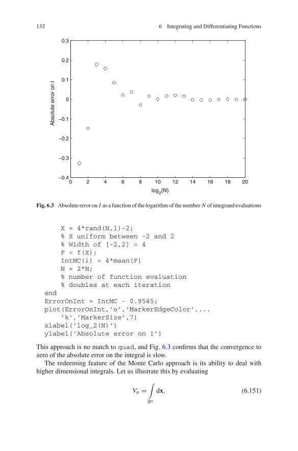
132 6 Integrating and Differentiating Functions

0 2 4 6 8 10 12 14 16 18 20−0.4

−0.3

−0.2

−0.1

0

0.1

0.2

0.3

log2(N)

Abs

olut

e er

ror

on I

Fig. 6.3 Absolute error on I as a function of the logarithm of the number N of integrand evaluations

X = 4*rand(N,1)-2;% X uniform between -2 and 2% Width of [-2,2] = 4F = f(X);IntMC(i) = 4*mean(F)N = 2*N;% number of function evaluation% doubles at each iteration

endErrorOnInt = IntMC - 0.9545;plot(ErrorOnInt,’o’,’MarkerEdgeColor’,...

’k’,’MarkerSize’,7)xlabel(’log_2(N)’)ylabel(’Absolute error on I’)

This approach is no match to quad, and Fig. 6.3 confirms that the convergence tozero of the absolute error on the integral is slow.

The redeeming feature of the Monte Carlo approach is its ability to deal withhigher dimensional integrals. Let us illustrate this by evaluating

Vn =∫

Bn

dx, (6.151)

6.7 MATLAB Examples 133

where Bn is the unit Euclidean ball in R

n ,

Bn = {x √ R

n such that ⊥x⊥2 � 1}. (6.152)

This can be carried out by the following script, where n is the dimension of theEuclidean space and V(i) the volume Vn as estimated from 2i pseudo random x’sin [−1, 1]×n .

clear allV = zeros(20,1);N = 1;%%%for i=1:20,

F = zeros(N,1);X = 2*rand(n,N)-1;% X uniform between -1 and 1for j=1:N,

x = X(:,j);if (norm(x,2)<=1)

F(j) = 1;end

endV(i) = mean(F)*2ˆn;N = 2*N;% Number of function evaluations% doubles at each iteration

end

Vn is the (hyper) volume of Bn , which can be computed exactly. The recurrence

Vn = 2π

nVn−2 (6.153)

can, for instance, be used to compute it for even n’s, starting from V2 = π . It impliesthat V6 = π3/6. Running our Monte Carlo script with n = 6; and adding

TrueV6 = (piˆ3)/6;RelErrOnV6 = 100*(V - TrueV6)/TrueV6;plot(RelErrOnV6,’o’,’MarkerEdgeColor’,...

’k’,’MarkerSize’,7)xlabel(’log_2(N)’)ylabel(’Relative error on V_6 (in %)’)

we get Fig. 6.4, which shows the evolution of the relative error on V6 as a functionof log2 N .

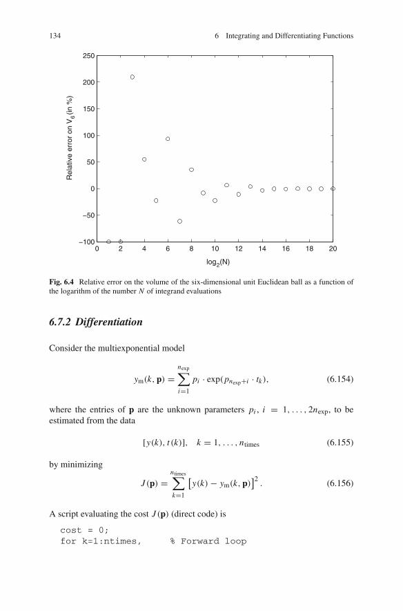
134 6 Integrating and Differentiating Functions

0 2 4 6 8 10 12 14 16 18 20−100

−50

0

50

100

150

200

250

log2(N)

Rel

ativ

e er

ror

on V

6 (in

%)

Fig. 6.4 Relative error on the volume of the six-dimensional unit Euclidean ball as a function ofthe logarithm of the number N of integrand evaluations

6.7.2 Differentiation

Consider the multiexponential model

ym(k, p) =nexp⎡

i=1

pi · exp(pnexp+i · tk), (6.154)

where the entries of p are the unknown parameters pi , i = 1, . . . , 2nexp, to beestimated from the data

[y(k), t (k)], k = 1, . . . , ntimes (6.155)

by minimizing

J (p) =ntimes⎡

k=1

[y(k) − ym(k, p)

]2. (6.156)

A script evaluating the cost J (p) (direct code) is

cost = 0;for k=1:ntimes, % Forward loop

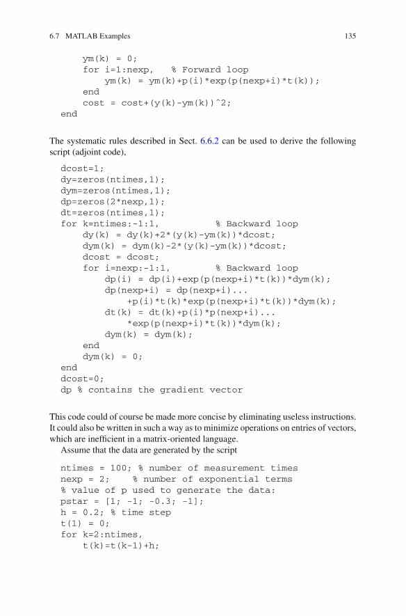
6.7 MATLAB Examples 135

ym(k) = 0;for i=1:nexp, % Forward loop

ym(k) = ym(k)+p(i)*exp(p(nexp+i)*t(k));endcost = cost+(y(k)-ym(k))ˆ2;

end

The systematic rules described in Sect. 6.6.2 can be used to derive the followingscript (adjoint code),

dcost=1;dy=zeros(ntimes,1);dym=zeros(ntimes,1);dp=zeros(2*nexp,1);dt=zeros(ntimes,1);for k=ntimes:-1:1, % Backward loop

dy(k) = dy(k)+2*(y(k)-ym(k))*dcost;dym(k) = dym(k)-2*(y(k)-ym(k))*dcost;dcost = dcost;for i=nexp:-1:1, % Backward loop

dp(i) = dp(i)+exp(p(nexp+i)*t(k))*dym(k);dp(nexp+i) = dp(nexp+i)...

+p(i)*t(k)*exp(p(nexp+i)*t(k))*dym(k);dt(k) = dt(k)+p(i)*p(nexp+i)...

*exp(p(nexp+i)*t(k))*dym(k);dym(k) = dym(k);

enddym(k) = 0;

enddcost=0;dp % contains the gradient vector

This code could of course be made more concise by eliminating useless instructions.It could also be written in such a way as to minimize operations on entries of vectors,which are inefficient in a matrix-oriented language.

Assume that the data are generated by the script

ntimes = 100; % number of measurement timesnexp = 2; % number of exponential terms% value of p used to generate the data:pstar = [1; -1; -0.3; -1];h = 0.2; % time stept(1) = 0;for k=2:ntimes,

t(k)=t(k-1)+h;

136 6 Integrating and Differentiating Functions

endfor k=1:ntimes,

y(k) = 0;for i=1:nexp,

y(k) = y(k)+pstar(i)*exp(pstar(nexp+i)*t(k));end

end

With these data, for p = (1.1,−0.9,−0.2,−0.9)T, the value of the gradient vectoras computed by the adjoint code is found to be

dp =7.847859612874749e+002.139461455801426e+003.086120784615719e+01-1.918927727244027e+00

In this simple example, the gradient of the cost is easy to compute analytically, as

∂ J

∂p= −2

ntimes⎡

k=1

[y(k) − ym(k, p)

] · ∂ym

∂p(k), (6.157)

with, for i = 1, . . . , nexp,

∂ym

∂pi(k, p) = exp(pnexp+i · tk), (6.158)

∂ym

∂pnexp+i(k, p) = tk · pi · exp(pnexp+i · tk). (6.159)

The results of the adjoint code can thus be checked by running the script

for i=1:nexp,for k=1:ntimes,

s(i,k) = exp(p(nexp+i)*t(k));s(nexp+i,k) = t(k)*p(i)*exp(p(nexp+i)*t(k));

endendfor i=1:2*nexp,

g(i) = 0;for k=1:ntimes,

g(i) = g(i)-2*(y(k)-ym(k))*s(i,k);end

endg % contains the gradient vector

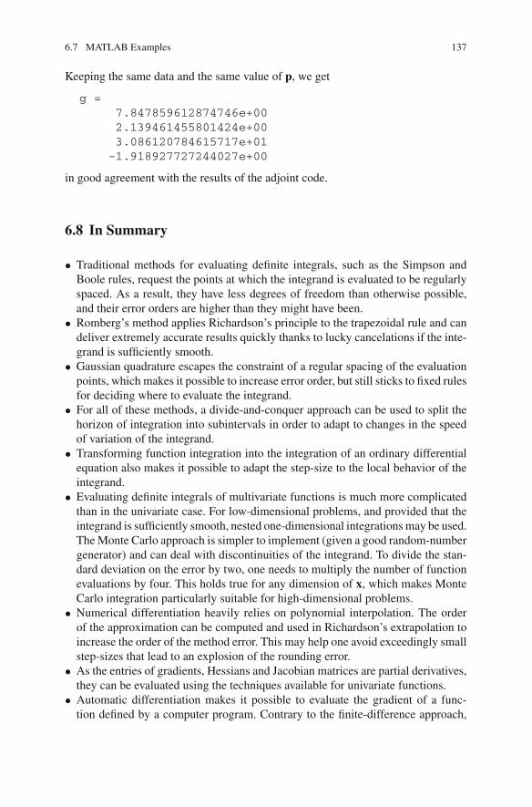
6.7 MATLAB Examples 137

Keeping the same data and the same value of p, we get

g =7.847859612874746e+002.139461455801424e+003.086120784615717e+01-1.918927727244027e+00

in good agreement with the results of the adjoint code.

6.8 In Summary

• Traditional methods for evaluating definite integrals, such as the Simpson andBoole rules, request the points at which the integrand is evaluated to be regularlyspaced. As a result, they have less degrees of freedom than otherwise possible,and their error orders are higher than they might have been.

• Romberg’s method applies Richardson’s principle to the trapezoidal rule and candeliver extremely accurate results quickly thanks to lucky cancelations if the inte-grand is sufficiently smooth.

• Gaussian quadrature escapes the constraint of a regular spacing of the evaluationpoints, which makes it possible to increase error order, but still sticks to fixed rulesfor deciding where to evaluate the integrand.

• For all of these methods, a divide-and-conquer approach can be used to split thehorizon of integration into subintervals in order to adapt to changes in the speedof variation of the integrand.

• Transforming function integration into the integration of an ordinary differentialequation also makes it possible to adapt the step-size to the local behavior of theintegrand.

• Evaluating definite integrals of multivariate functions is much more complicatedthan in the univariate case. For low-dimensional problems, and provided that theintegrand is sufficiently smooth, nested one-dimensional integrations may be used.The Monte Carlo approach is simpler to implement (given a good random-numbergenerator) and can deal with discontinuities of the integrand. To divide the stan-dard deviation on the error by two, one needs to multiply the number of functionevaluations by four. This holds true for any dimension of x, which makes MonteCarlo integration particularly suitable for high-dimensional problems.

• Numerical differentiation heavily relies on polynomial interpolation. The orderof the approximation can be computed and used in Richardson’s extrapolation toincrease the order of the method error. This may help one avoid exceedingly smallstep-sizes that lead to an explosion of the rounding error.

• As the entries of gradients, Hessians and Jacobian matrices are partial derivatives,they can be evaluated using the techniques available for univariate functions.

• Automatic differentiation makes it possible to evaluate the gradient of a func-tion defined by a computer program. Contrary to the finite-difference approach,

138 6 Integrating and Differentiating Functions

automatic differentiation introduces no method error. Backward differentiationrequires less flops that forward differentiation, especially if dim x is large, butis more complicated to implement and may require a large memory space. Bothtechniques extend to the numerical evaluation of higher order derivatives.

References

1. Jazwinski, A.: Stochastic Processes and Filtering Theory. Academic Press, New York (1970)2. Borrie, J.: Stochastic Systems for Engineers. Prentice-Hall, Hemel Hempstead (1992)3. Gander, W., Gautschi, W.: Adaptive quadrature—revisited. BIT 40(1), 84–101 (2000)4. Fortin, A.: Numerical Analysis for Engineers. Ecole Polytechnique de Montréal, Montréal

(2009)5. Stoer, J., Bulirsch, R.: Introduction to Numerical Analysis. Springer, New York (1980)6. Golub, G., Welsch, J.: Calculation of Gauss quadrature rules. Math. Comput. 23(106), 221–230

(1969)7. Lowan, A., Davids, N., Levenson, A.: Table of the zeros of the Legendre polynomials of order

1–16 and the weight coefficients for Gauss’ mechanical quadrature formula. Bull. Am. Math.Soc. 48(10), 739–743 (1942)

8. Lowan, A., Davids, N., Levenson, A.: Errata to “Table of the zeros of the Legendre polynomialsof order 1–16 and the weight coefficients for Gauss’ mechanical quadrature formula”. Bull.Am. Math. Soc. 49(12), 939–939 (1943)

9. Knuth, D.: The Art of Computer Programming: 2 Seminumerical Algorithms, 3rd edn. Addison-Wesley, Reading (1997)

10. Press, W., Flannery, B., Teukolsky, S., Vetterling, W.: Numerical Recipes. Cambridge Univer-sity Press, Cambridge (1986)

11. Moler, C.: Numerical Computing with MATLAB, revised, reprinted edn. SIAM, Philadelphia(2008)

12. Robert, C., Casella, G.: Monte Carlo Statistical Methods. Springer, New York (2004)13. Morokoff, W., Caflisch, R.: Quasi-Monte Carlo integration. J. Comput. Phys. 122, 218–230

(1995)14. Owen, A.: Monte Carlo variance of scrambled net quadratures. SIAM J. Numer. Anal. 34(5),

1884–1910 (1997)15. Gilbert, J., Vey, G.L., Masse, J.: La différentiation automatique de fonctions représentées par

des programmes. Technical Report 1557, INRIA (1991)16. Griewank, A., Corliss, G. (eds.): Automatic Differentiation of Algorithms: Theory Implemen-

tation and Applications. SIAM, Philadelphia (1991)17. Speelpening, B.: Compiling fast partial derivatives of functions given by algorithms. Ph.D.

thesis, Department of Computer Science, University of Illinois, Urbana Champaign (1980)18. Hammer, R., Hocks, M., Kulisch, U., Ratz, D.: C++ Toolbox for Verified Computing. Springer,

Berlin (1995)19. Rall, L., Corliss, G.: Introduction to automatic differentiation. In: Bertz, M., Bischof, C.,

Corliss, G., Griewank, A. (eds.) Computational Differentiation Techniques, Applications, andTools. SIAM, Philadelphia (1996)

20. Nocedal, J., Wright, S.: Numerical Optimization. Springer, New York (1999)21. Griewank, A., Walther, A.: Principles and Techniques of Algorithmic Differentiation, 2nd edn.

SIAM, Philadelphia (2008)

Chapter 7Solving Systems of Nonlinear Equations

7.1 What Are the Differences with the Linear Case?

As in Chap. 3, the number of scalar equations is assumed here to be equal to thenumber of scalar unknowns. Recall that in the linear case there are only three possi-bilities:

• there is no solution, because the equations are incompatible,• the solution is unique,• the solution set is a continuum, because at least one equation can be deduced from

the others by linear combination, so there are not enough independent equations.

For nonlinear equations, there are new possibilities:

• a single scalar equation in one unknown may have no solution (Fig. 7.1),• there may be several isolated solutions (Fig. 7.2).

We assume that there exists at least one solution and that the solution set is finite(it may be a singleton but we may not know about that).

The methods presented here try to find solutions in this finite set, without anyguarantee of success or exhaustivity. Guaranteed numerical methods based oninterval analysis that look for all the solutions are alluded to in Sect. 14.5.2.3.(See, e.g., [1, 2] for more details.)

É. Walter, Numerical Methods and Optimization, 139DOI: 10.1007/978-3-319-07671-3_7,© Springer International Publishing Switzerland 2014

140 7 Solving Systems of Nonlinear Equations

f(x)

x0

Fig. 7.1 A single nonlinear equation f (x) = 0, with no solution

x

f(x)

0

Fig. 7.2 A nonlinear equation f (x) = 0 with several isolated solutions

7.2 Examples

Example 7.1 Equilibrium points of nonlinear differential equationsThe chemical reactions taking place inside a constant-temperature continuous

stirred tank reactor (CSTR) can be described by a system of nonlinear ordinarydifferential equations

x = f(x), (7.1)

7.2 Examples 141

where x is a vector of concentrations. The equilibrium points of the reactor satisfy

f(x) = 0. (7.2)

�

Example 7.2 Stewart-Gough platformsIf you have seen a flight simulator used for training pilots of commercial or

military aircraft, then you have seen a Stewart-Gough platform. Amusement parksalso employ these structures. They consist of two rigid plates, connected by sixhydraulic jacks, the lengths of which can be controlled to change the position of oneplate relative to the other. In a flight simulator, the base plate stays on the groundwhile the seat of the pilot is fixed to the mobile plate. Steward-Gough platformsare examples of parallel robots, as the six jacks act in parallel to move the mobileplate whereas the effectors of humanoid arms act in series. Parallel robots are anattractive alternative to serial robots for tasks that require precision and power, buttheir control is more complex. We are concerned here with a very basic problem,namely the computation of the possible positions of the mobile plate relative to thebase knowing the geometry of the platform and the lengths of the jacks. These lengthsare assumed to be constant, so this is a static problem.

This problem translates into a system of six nonlinear equations in six unknowns(three Euler angles and the three coordinates of the position of a given point of themobile plate in the referential of the base plate). These equations involve sines andcosines, and one may prefer to consider a system of nine polynomial equations innine unknowns. The unknowns are then the sines and cosines of the Euler anglesand the three coordinates of the position of a given point of the mobile plate in thereferential of the base plate, while the additional equations are

sin2(∂i ) + cos2(∂i ) = 1, i = 1, 2, 3, (7.3)

with ∂i the i th Euler angle. Computing all the solutions of such a system of equa-tions is difficult, especially if one is interested only in the real solutions. That iswhy this problem has become a benchmark in computer algebra [3], which can alsobe solved numerically in an approximate but guaranteed way by interval analysis[4]. The methods described in this chapter try, more modestly, to find some of thesolutions. �

7.3 One Equation in One Unknown

Most methods for solving systems of nonlinear equations in several unknowns (ormultivariate systems) are extensions of methods for one equation in one unknown,so this section might serve as an introduction to the more general case considered inSect. 7.4.

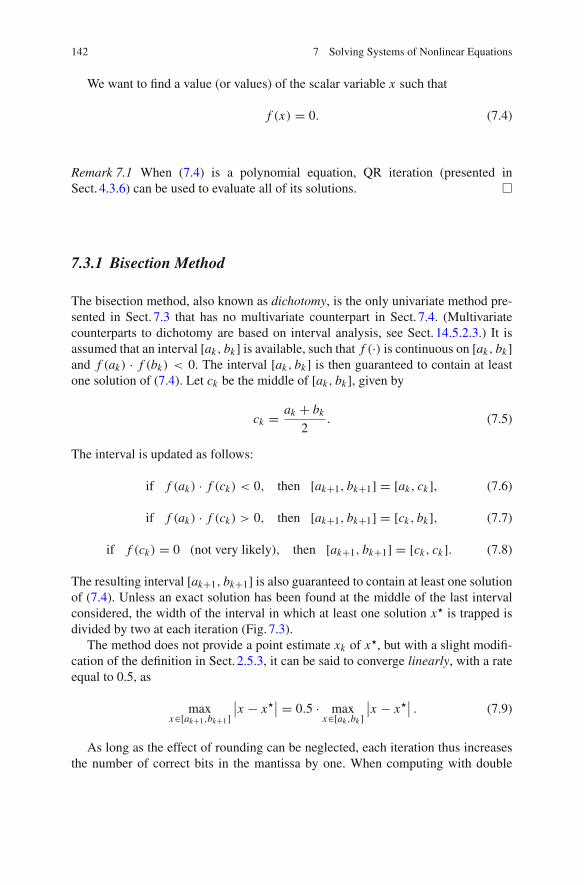
142 7 Solving Systems of Nonlinear Equations

We want to find a value (or values) of the scalar variable x such that

f (x) = 0. (7.4)

Remark 7.1 When (7.4) is a polynomial equation, QR iteration (presented inSect. 4.3.6) can be used to evaluate all of its solutions. �

7.3.1 Bisection Method

The bisection method, also known as dichotomy, is the only univariate method pre-sented in Sect. 7.3 that has no multivariate counterpart in Sect. 7.4. (Multivariatecounterparts to dichotomy are based on interval analysis, see Sect. 14.5.2.3.) It isassumed that an interval [ak, bk] is available, such that f (·) is continuous on [ak, bk]and f (ak) · f (bk) < 0. The interval [ak, bk] is then guaranteed to contain at leastone solution of (7.4). Let ck be the middle of [ak, bk], given by

ck = ak + bk

2. (7.5)

The interval is updated as follows:

if f (ak) · f (ck) < 0, then [ak+1, bk+1] = [ak, ck], (7.6)

if f (ak) · f (ck) > 0, then [ak+1, bk+1] = [ck, bk], (7.7)

if f (ck) = 0 (not very likely), then [ak+1, bk+1] = [ck, ck]. (7.8)

The resulting interval [ak+1, bk+1] is also guaranteed to contain at least one solutionof (7.4). Unless an exact solution has been found at the middle of the last intervalconsidered, the width of the interval in which at least one solution x� is trapped isdivided by two at each iteration (Fig. 7.3).

The method does not provide a point estimate xk of x�, but with a slight modifi-cation of the definition in Sect. 2.5.3, it can be said to converge linearly, with a rateequal to 0.5, as

maxx√[ak+1,bk+1]

∣∣x − x�∣∣ = 0.5 · max

x√[ak ,bk ]∣∣x − x�

∣∣ . (7.9)

As long as the effect of rounding can be neglected, each iteration thus increasesthe number of correct bits in the mantissa by one. When computing with double

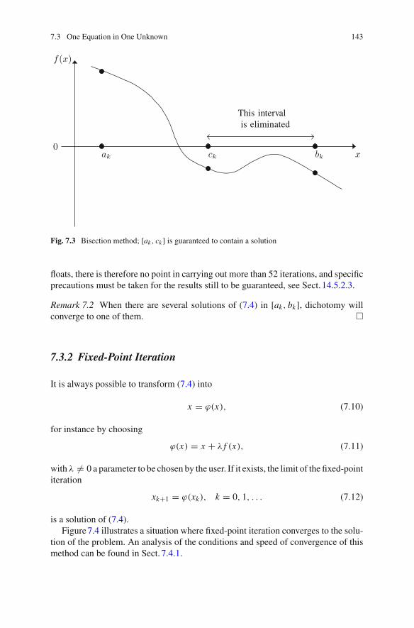
7.3 One Equation in One Unknown 143

f(x)

xak ck bk

This intervalis eliminated

0

Fig. 7.3 Bisection method; [ak , ck ] is guaranteed to contain a solution

floats, there is therefore no point in carrying out more than 52 iterations, and specificprecautions must be taken for the results still to be guaranteed, see Sect. 14.5.2.3.

Remark 7.2 When there are several solutions of (7.4) in [ak, bk], dichotomy willconverge to one of them. �

7.3.2 Fixed-Point Iteration

It is always possible to transform (7.4) into

x = δ(x), (7.10)

for instance by choosing

δ(x) = x + α f (x), (7.11)

with α ∇= 0 a parameter to be chosen by the user. If it exists, the limit of the fixed-pointiteration

xk+1 = δ(xk), k = 0, 1, . . . (7.12)

is a solution of (7.4).Figure 7.4 illustrates a situation where fixed-point iteration converges to the solu-

tion of the problem. An analysis of the conditions and speed of convergence of thismethod can be found in Sect. 7.4.1.

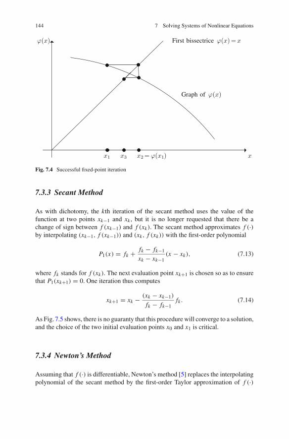
144 7 Solving Systems of Nonlinear Equations

x

ϕ(x) First bissectrice ϕ(x)= x

Graph of ϕ(x)

x1 x3 x2= ϕ(x1)

Fig. 7.4 Successful fixed-point iteration

7.3.3 Secant Method

As with dichotomy, the kth iteration of the secant method uses the value of thefunction at two points xk−1 and xk , but it is no longer requested that there be achange of sign between f (xk−1) and f (xk). The secant method approximates f (·)by interpolating (xk−1, f (xk−1)) and (xk, f (xk)) with the first-order polynomial

P1(x) = fk + fk − fk−1

xk − xk−1(x − xk), (7.13)

where fk stands for f (xk). The next evaluation point xk+1 is chosen so as to ensurethat P1(xk+1) = 0. One iteration thus computes

xk+1 = xk − (xk − xk−1)

fk − fk−1fk . (7.14)

As Fig. 7.5 shows, there is no guaranty that this procedure will converge to a solution,and the choice of the two initial evaluation points x0 and x1 is critical.

7.3.4 Newton’s Method

Assuming that f (·) is differentiable, Newton’s method [5] replaces the interpolatingpolynomial of the secant method by the first-order Taylor approximation of f (·)

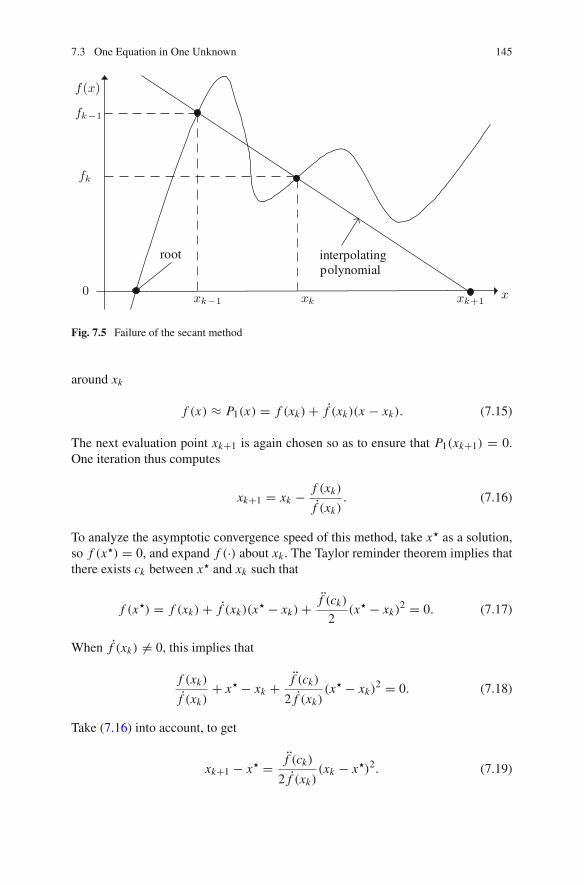
7.3 One Equation in One Unknown 145

xk xk+1xk−1x

f(x)

fk−1

fk

interpolatingpolynomial

root

0

Fig. 7.5 Failure of the secant method

around xk

f (x) → P1(x) = f (xk) + f (xk)(x − xk). (7.15)

The next evaluation point xk+1 is again chosen so as to ensure that P1(xk+1) = 0.One iteration thus computes

xk+1 = xk − f (xk)

f (xk). (7.16)

To analyze the asymptotic convergence speed of this method, take x� as a solution,so f (x�) = 0, and expand f (·) about xk . The Taylor reminder theorem implies thatthere exists ck between x� and xk such that

f (x�) = f (xk) + f (xk)(x� − xk) + f (ck)

2(x� − xk)

2 = 0. (7.17)

When f (xk) ∇= 0, this implies that

f (xk)

f (xk)+ x� − xk + f (ck)

2 f (xk)(x� − xk)

2 = 0. (7.18)

Take (7.16) into account, to get

xk+1 − x� = f (ck)

2 f (xk)(xk − x�)2. (7.19)

146 7 Solving Systems of Nonlinear Equations

0 x

1

2

3

f (x)

x1 x0 x2

Fig. 7.6 Failure of Newton’s method

When xk and x� are close enough,

∣∣xk+1 − x�∣∣ →

∣∣∣∣f (x�)

2 f (x�)

∣∣∣∣⎡xk − x�

⎢2, (7.20)

provided that f (·) has continuous, bounded first and second derivatives in the neigh-borhood of x� with f (x�) ∇= 0. Convergence of xk toward x� is then quadratic. Thenumber of correct digits in the solution should approximately double at each itera-tion until rounding error becomes predominant. This is much better than the linearconvergence of the bisection method, but there are drawbacks:

• there is no guarantee that Newton’s method will converge to a solution (seeFig. 7.6),

• f (xk) must be evaluated,• the choice of the initial evaluation point x0 is critical.

Rewrite (7.20) as∣∣xk+1 − x�

∣∣ → ρ⎡xk − x�

⎢2, (7.21)

with

ρ =∣∣∣∣

f (x�)

2 f (x�)

∣∣∣∣ . (7.22)

Equation (7.21) implies that

∣∣ρ(xk+1 − x�)∣∣ → [ρ ⎡

xk − x�⎢]2. (7.23)

7.3 One Equation in One Unknown 147

This suggests wishing that |ρ(x0 − x�)| < 1, i.e.,

∣∣x0 − x�∣∣ <

1

ρ=

∣∣∣∣2 f (x�)

f (x�)

∣∣∣∣ , (7.24)

although the method may still work when this condition is not satisfied.

Remark 7.3 Newton’s method runs into trouble when f (x�) = 0, which happenswhen the root x� is multiple, i.e., when

f (x) = (x − x�)m g(x), (7.25)

with g(x�) ∇= 0 and m > 1. Its (asymptotic) convergence speed is then only linear.When the degree of multiplicity m is known, quadratic convergence speed can berestored by replacing (7.16) by

xk+1 = xk − mf (xk)

f (xk). (7.26)

When m is not known, or when f (·) has several multiple roots, one may insteadreplace f (·) in (7.16) by h(·), with

h(x) = f (x)

f (x), (7.27)

as all the roots of h(·) are simple. �

One way to escape (some) convergence problems is to use a damped Newtonmethod

xk+1 = xk − αkf (xk)

f (xk), (7.28)

where the positive damping factor αk is normally equal to one, but decreases when theabsolute value of f (xk+1) turns out to be greater than that of f (xk), a sure indicationthat the displacement σx = xk+1 − xk was too large for the first-order Taylorexpansion to be a valid approximation of the function. In this case, of course, xk+1must be rejected to the benefit of xk . This ensures, at least mathematically, that | f (xk)|will decrease monotonically along the iterations, but it may still not converge to zero.

Remark 7.4 The secant step (7.14) can be viewed as a Newton step (7.16) wheref (xk) is approximated by a first-order backward finite difference. Under the samehypotheses as for Newton’s method, a more involved error analysis [6] shows that

∣∣xk+1 − x�∣∣ → ρ

⇒5−12

∣∣xk − x�∣∣ 1+⇒

52 . (7.29)

148 7 Solving Systems of Nonlinear Equations

The asymptotic convergence speed of the secant method to a simple root x� is thusnot quadratic, but still superlinear, as the golden number (1 + ⇒

5)/2 is such that

1 <1 + ⇒

5

2→ 1.618 < 2. (7.30)

Just as with Newton’s method, the asymptotic convergence speed becomes linear ifthe root x� is multiple [7].

Recall that the secant method does not requires the evaluation of f (xk), so eachiteration is less expensive than with Newton’s method. �

7.4 Multivariate Systems

Consider now a set of n scalar equations in n scalar unknowns, with n > 1. It canbe written more concisely as

f(x) = 0, (7.31)

where f(·) is a function from Rn to R

n . A number of interesting survey papers onthe solution of (7.31) are in the special issue [8]. A concise practical guide to thesolution of nonlinear equations by Newton’s method and its variants is [9].

7.4.1 Fixed-Point Iteration

As in the univariate case, (7.31) can always be transformed into

x = ϕϕϕ(x), (7.32)

for instance by posing

ϕϕϕ(x) = x + αf(x), (7.33)

with α ∇= 0 some scalar parameter to be chosen by the user. If it exists, the limit ofthe fixed-point iteration

xk+1 = ϕϕϕ(xk), k = 0, 1, . . . (7.34)

is a solution of (7.31).This method will converge to the solution x� if ϕϕϕ(·) is contracting, i.e., such that

∈ν < 1 : ∀ (x1, x2) , ||ϕϕϕ(x1) − ϕϕϕ(x2)|| < ν||x1 − x2||, (7.35)

and the smaller ν is, the better.

7.4 Multivariate Systems 149

For x1 = xk and x2 = x�, (7.35) becomes

⊂xk+1 − x�⊂ < ν⊂xk − x�⊂, (7.36)

so convergence is linear, with rate ν.

Remark 7.5 The iterative methods of Sect. 3.7.1 are fixed-point methods, thus slow.This is one more argument in favor of Krylov subspace methods, presented inSect. 3.7.2., which converge in at most dim x iterations when computation is car-ried out exactly. �

7.4.2 Newton’s Method

As in the univariate case, f(·) is approximated by its first-order Taylor expansionaround xk

f(x) → f(xk) + J(xk)(x − xk), (7.37)

where J(xk) is the (n × n) Jacobian matrix of f(·) evaluated at xk

J(xk) = βfβxT (xk), (7.38)

with entries

ji,l = β fi

βxl(xk). (7.39)

The next evaluation point xk+1 is chosen so as to make the right-hand side of (7.37)equal to zero. One iteration thus computes

xk+1 = xk − J−1(xk)f(xk). (7.40)

Of course, the Jacobian matrix is not inverted. Instead, the corrective term

σxk = xk+1 − xk (7.41)

is evaluated by solving the linear system

J(xk)σxk = −f(xk), (7.42)

and the next estimate of the solution vector is taken as

xk+1 = xk + σxk . (7.43)

150 7 Solving Systems of Nonlinear Equations

Remark 7.6 The condition number of J(xk) is indicative of the local difficulty ofthe problem, which depends on the value of xk . Even if the condition number of theJacobian matrix at an actual solution vector is not too large, it may take very largevalues for some values of xk along the trajectory of the algorithm. �

The properties of Newton’s method in the multivariate case are similar to thoseof the univariate case. Under the following hypotheses

• f(·) is continuously differentiable in an open convex domain D (H1),• there exists x� in D such that f(x�) = 0 and J(x�) is invertible (H2),• J(·) satisfies a Lipschitz condition at x�, i.e., there exists a constant κ such that

⊂J(x) − J(x�)⊂ � κ⊂x − x�⊂ (H3),

asymptotic convergence speed is quadratic provided that x0 is close enough to x�.In practice, the method may fail to converge to a solution and initialization remains

critical. Again, some divergence problems can be avoided by using a damped Newtonmethod,

xk+1 = xk + αkσxk, (7.44)

where the positive damping factor αk is initially set to one, unless⎣⎣f(xk+1)

⎣⎣ turnsout to be larger than

⎣⎣f(xk)⎣⎣, in which case xk+1 is rejected and αk reduced (typically

halved until⎣⎣f(xk+1)

⎣⎣ <⎣⎣f(xk)

⎣⎣).

Remark 7.7 In the special case of a system of linear equations Ax = b, with Ainvertible,

f(x) = Ax − b and J = A, so xk+1 = A−1b. (7.45)

Newton’s method thus evaluates the unique solution in a single step. �

Remark 7.8 Newton’s method also plays a key role in optimization, seeSect. 9.3.4.2. �

7.4.3 Quasi–Newton Methods

Newton’s method may be simplified by replacing the Jacobian matrix J(xk) in (7.42)by J(x0), which is then computed and factored only once. The resulting method,known as a chord method, may diverge where Newton’s method would converge.Quasi-Newton methods address this difficulty by updating an estimate of the Jacobianmatrix (or of its inverse) at each iteration [10]. They also play an important role inunconstrained optimization, see Sect. 9.3.4.5.

In the context of nonlinear equations, the most popular quasi-Newton method isBroyden’s [11]. It may be seen as a generalization of the secant method of Sect. 7.3.3

7.4 Multivariate Systems 151

where f (xk) was approximated by a finite difference (see Remark 7.4). The approx-imation

f (xk) → fk − fk−1

xk − xk−1, (7.46)

becomes

J(xk+1)σx → σf, (7.47)

where

σx = xk+1 − xk, (7.48)

σf = f(xk+1) − f(xk). (7.49)

The information provided by (7.47) is used to update an approximation Jk ofJ(xk+1) as

Jk+1 = Jk + C(σx,σf), (7.50)

where C(σx,σf) is a rank-one correction matrix (i.e., the product of a column vectorby a row vector on its right). For

C(σx,σf) = (σf − Jkσx)

σxTσxσxT, (7.51)

it is trivial to check that the update formula (7.50) ensures

Jk+1σx = σf, (7.52)

as suggested by (7.47). Equation (7.52) is so central to quasi-Newton methodsthat it has been dubbed the quasi-Newton equation. Moreover, for any w such thatσxTw = 0,

Jk+1w = Jkw, (7.53)

so the approximation is unchanged on the orthogonal complement of σx.Another way of arriving at the same rank-one correction matrix is to look for

the matrix Jk+1 that satisfies (7.52) while being the closest to Jk for the Frobeniusnorm [10].

It is more interesting, however, to update an approximation M = J−1 of theinverse of the Jacobian matrix, in order to avoid having to solve a system of linearequations at each iteration. Provided that Jk is invertible and 1 + vTJ−1

k u ∇= 0, theBartlett-Sherman-Morrison formula [12] states that

(Jk + uvT)−1 = J−1k − J−1

k uvTJ−1k

1 + vTJ−1k u

. (7.54)

152 7 Solving Systems of Nonlinear Equations

To update the estimate of J−1⎡xk+1

⎢according to

Mk+1 = Mk − C∞(σx,σf), (7.55)

it suffices to take

u = (σf − Jkσx)

⊂σx⊂2(7.56)

and

v = σx⊂σx⊂2

(7.57)

in (7.51). Since

J−1k u = Mkσf − σx

⊂σx⊂2, (7.58)

it is not necessary to know Jk to use (7.54), and

C∞(σx,σf) = J−1k uvTJ−1

k

1 + vTJ−1k u

,

=(Mkσf −σx)σxTMk

σxTσx

1 + σxT(Mkσf −σx)

σxTσx

,

= (Mkσf − σx)σxTMk

σxTMkσf. (7.59)

The correction term C∞(σx,σf) is thus also a rank-one matrix. As with Newton’smethod, a damping procedure is usually employed, such that

σx = αd, (7.60)

where the search direction d is taken as in Newton’s method, with J−1(xk) replacedby Mk , so

d = −Mkf(xk). (7.61)

The correction term then becomes

C∞(σx,σf) = (Mkσf − αd)dTMk

dTMkσf. (7.62)

In summary, starting from k = 0 and the pair (x0, M0), (M0 might be taken asJ−1(x0), or more simply as the identity matrix), the method proceeds as follows:

1. Compute fk = f⎡xk

⎢.

2. Compute d = −Mkfk .

7.4 Multivariate Systems 153

3. Find⎤α such that⊂f(xk +⎤αd)⊂ < ⊂fk⊂ (7.63)

and take

xk+1 = xk +⎤αd, (7.64)

fk+1 = f(xk+1).

4. Compute σf = fk+1 − fk .5. Compute

Mk+1 = Mk − (Mkσf −⎤αd)dTMk

dTMkσf. (7.65)

6. Increment k by one and repeat from Step 2.

Under the same hypotheses (H1) to (H3) under which Newton’s method con-verges quadratically, Broyden’s method converges superlinearly (provided that x0

is sufficiently close to x� and M0 sufficiently close to J−1(x�)) [10]. This does notnecessarily mean that Newton’s method requires less computation, as Broyden’siterations are often much simpler that Newton’s.

7.5 Where to Start From?

All the methods presented in this chapter for solving systems of nonlinear equationsare iterative. With the exception of the bisection method, which is based on intervalreasoning and guaranteed to improve the precision with which a solution is localized,they start from some initial evaluation point (or points for the secant method) tocompute new evaluation points that are hopefully closer to one of the solutions.Even if a good approximation of a solution is known a priori, and unless computingtime forbids it, it is then a good idea to try several initial points picked at random inthe domain of interest X. This strategy, known as multistart, is a particularly simpleattempt at finding solutions by random search. Although it may find all the solutions,there is no guarantee that it will do so.

Remark 7.9 Continuation methods, also called homotopy methods, are an interestingalternative to multistart. They slowly transform the known solutions of an easy systemof equations e(x) = 0 into those of (7.31). For this purpose, they solve

hα(x) = 0, (7.66)

wherehα(x) = αf(x) + (1 − α)e(x), (7.67)

154 7 Solving Systems of Nonlinear Equations

with α varying from zero to one. In practice, it is often necessary to allow α todecrease temporarily on the road from zero to one, and implementation is not trivial.See, e.g., [13] for an introduction. �

7.6 When to Stop?

Iterative algorithms cannot be allowed to run forever (especially in a context ofmultistart, where they might be executed many times). Stopping criteria must thusbe specified. Mathematically, one should stop when a solution has been reached,i.e., when f(x) = 0. From the point of view of numerical computation, this doesnot make sense and one may decide to stop instead when

⎣⎣f(xk)⎣⎣ < δ, where δ is

a positive threshold to be chosen by the user, or when⎣⎣f(xk) − f(xk−1)

⎣⎣ < δ. Thefirst of these stopping criteria may never be met if δ is too small or if x0 was badlychosen, which provides a rationale for using the second one.

With either of these strategies, the number of iterations will change drastically fora given threshold if the equations are arbitrarily multiplied by a very large or verysmall real number.

One may prefer a stopping criterion that does not present this property, such asstopping when ⎣⎣f(xk)

⎣⎣ < δ⎣⎣f(x0)

⎣⎣ (7.68)

(which may never happen) or when

⎣⎣f(xk) − f(xk−1)⎣⎣ < δ

⎣⎣f(xk) + f(xk−1)⎣⎣. (7.69)

One may also decide to stop when

⎣⎣xk − xk−1⎣⎣

⎣⎣xk⎣⎣ + realmin

� eps, (7.70)

or when ⎣⎣f⎡xk

⎢ − f⎡xk−1

⎢⎣⎣⎣⎣f

⎡xk

⎢⎣⎣ + realmin� eps, (7.71)

where eps is the relative precision of the floating-point representation employed(also called machine epsilon) and realmin is the smallest strictly positive normal-ized floating-point number, put in the denominators of the left-hand sides of (7.70)and (7.71) to protect against divisions by zero. When double floats are used, as inMATLAB, IEEE 754 compliant computers have

eps → 2.22 · 10−16 (7.72)

7.6 When to Stop? 155

andrealmin → 2.225 · 10−308. (7.73)

A last interesting idea is to stop when there is no longer any significant digit in theevaluation of f(xk), i.e., when one is no longer sure that a solution has not beenreached. This requires methods for assessing the precision of numerical results, suchas described in Chap. 14.

Several stopping criteria may be combined, and one should also specify a maxi-mum number of iterations, if only as a safety measure against badly designed othertests.

7.7 MATLAB Examples

7.7.1 One Equation in One Unknown

When f (x) = x2 − 3, the equation f (x) = 0 has two real solutions for x , namely

x = ±⇒3 → ±1.732050807568877. (7.74)

Let us solve it with the four methods presented in Sect. 7.3.

7.7.1.1 Using Newton’s Method

A very primitive script implementing (7.16) is

clear allKmax = 10;x = zeros(Kmax,1);x(1) = 1;f = @(x) x.ˆ2-3;fdot = @(x) 2*x;for k=1:Kmax,

x(k+1) = x(k)-f(x(k))/fdot(x(k));endx

It produces

x =1.000000000000000e+002.000000000000000e+001.750000000000000e+001.732142857142857e+00

156 7 Solving Systems of Nonlinear Equations

1.732050810014728e+001.732050807568877e+001.732050807568877e+001.732050807568877e+001.732050807568877e+001.732050807568877e+001.732050807568877e+00

Although an accurate solution is obtained very quickly, this script can be improvedin a number of ways.

First, there is no point in iterating when the solution has been reached (at least up tothe precision of the floating-point representation employed). A more sophisticatedstopping rule than just a maximum number of iterations must thus be specified. Onemay, for instance, use (7.70) and replace the loop in the previous script by

for k=1:Kmax,x(k+1) = x(k)-f(x(k))/fdot(x(k));if ((abs(x(k+1)-x(k)))/(abs(x(k+1)+realmin))<=eps)

breakend

end

The new loop terminates after only six iterations.A second improvement is to implement multistart, so as to look for other solutions.

One may write, for instance,

clear allSmax = 10; % number of startsKmax = 10; % max number of iterations per startInit = 2*rand(Smax,1)-1; % Between -1 and 1x = zeros(Kmax,1);Solutions = zeros(Smax,1);f = @(x) x.ˆ2-3;fdot = @(x) 2*x;for i=1:Smax,

x(1) = Init(i);for k=1:Kmax,

x(k+1) = x(k)-f(x(k))/fdot(x(k));if ((abs(x(k+1)-x(k)))/...

(abs(x(k+1)+realmin))<=eps)break

endendSolutions(i) = x(k+1);

endSolutions

7.7 MATLAB Examples 157

a typical run of which yields

Solutions =-1.732050807568877e+00-1.732050807568877e+00-1.732050807568877e+001.732050807568877e+001.732050807568877e+001.732050807568877e+001.732050807568877e+001.732050807568877e+00-1.732050807568877e+001.732050807568877e+00

The two solutions have thus been located (recall that there is no guarantee thatmultistart would succeed to do so on a more complicated problem). Damping wasnot necessary on this simple problem.

7.7.1.2 Using the Secant Method

It is a simple matter to transform the previous script into one implementing (7.14),such as

clear allSmax = 10; % number of startsKmax = 20; % max number of iterations per startInit = 2*rand(Smax,1)-1; % Between -1 and 1x = zeros(Kmax,1);Solutions = zeros(Smax,1);f = @(x) x.ˆ2-3;for i=1:Smax,

x(1) = Init(i);x(2) = x(1)+0.1; % Not very fancy...for k=2:Kmax,

x(k+1) = x(k) - (x(k)-x(k-1))...*f(x(k))/(f(x(k))-f(x(k-1)));

if ((abs(x(k+1)-x(k)))/...(abs(x(k+1)+realmin))<=eps)

breakend

endSolutions(i) = x(k+1);

endSolutions

158 7 Solving Systems of Nonlinear Equations

The inner loop typically breaks after 12 iterations, which confirms that the secantmethod is slower than Newton’s, and a typical run yields

Solutions =1.732050807568877e+001.732050807568877e+00-1.732050807568877e+00-1.732050807568877e+00-1.732050807568877e+001.732050807568877e+00-1.732050807568877e+001.732050807568877e+00-1.732050807568877e+001.732050807568877e+00

so the secant method with multstart is able to find both solutions with the sameaccuracy as Newton’s.

7.7.1.3 Using Fixed-Point Iteration

Let us tryxk+1 = xk + α(x2

k − 3), (7.75)

as implemented in the script

clear alllambda = 0.5 % tunableKmax = 50; % max number of iterationsf = @(x) x.ˆ2-3;x = zeros(Kmax+1,1);x(1) = 2*rand(1)-1; % Between -1 and 1for k=1:Kmax,

x(k+1) = x(k)+lambda*f(x(k));endSolution = x(Kmax+1)

It requires some fiddling to find a value of α that ensures convergence to an approx-imate solution. For α = 0.5, convergence is achieved toward an approximation of−⇒

3 whereas for α = −0.5 it is achieved toward an approximation of⇒

3. In bothcases, convergence is even slower than with the secant method. With α = 0.5, forinstance, 50 iterations of a typical run yielded

Solution = -1.732050852324972e+00

and 100 iterations

Solution = -1.732050807568868e+00

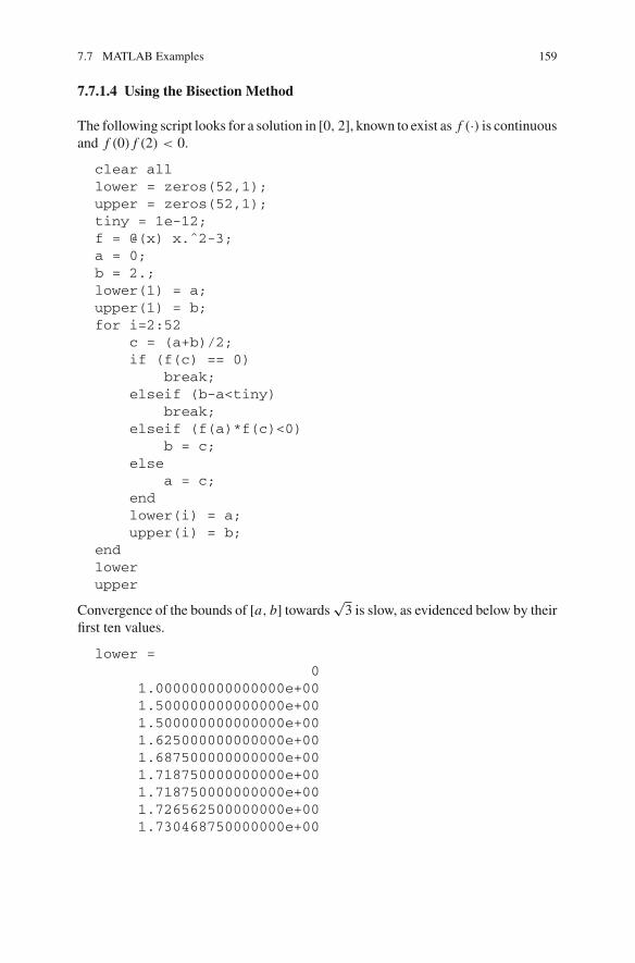
7.7 MATLAB Examples 159

7.7.1.4 Using the Bisection Method

The following script looks for a solution in [0, 2], known to exist as f (·) is continuousand f (0) f (2) < 0.

clear alllower = zeros(52,1);upper = zeros(52,1);tiny = 1e-12;f = @(x) x.ˆ2-3;a = 0;b = 2.;lower(1) = a;upper(1) = b;for i=2:52

c = (a+b)/2;if (f(c) == 0)

break;elseif (b-a<tiny)

break;elseif (f(a)*f(c)<0)

b = c;else

a = c;endlower(i) = a;upper(i) = b;

endlowerupper

Convergence of the bounds of [a, b] towards⇒

3 is slow, as evidenced below by theirfirst ten values.

lower =0

1.000000000000000e+001.500000000000000e+001.500000000000000e+001.625000000000000e+001.687500000000000e+001.718750000000000e+001.718750000000000e+001.726562500000000e+001.730468750000000e+00

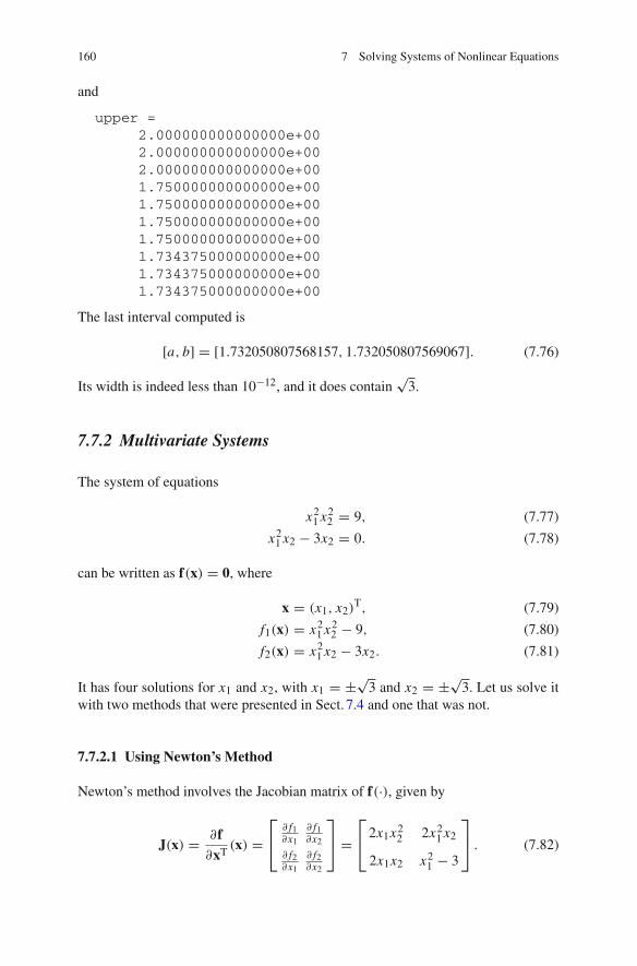
160 7 Solving Systems of Nonlinear Equations

and

upper =2.000000000000000e+002.000000000000000e+002.000000000000000e+001.750000000000000e+001.750000000000000e+001.750000000000000e+001.750000000000000e+001.734375000000000e+001.734375000000000e+001.734375000000000e+00

The last interval computed is

[a, b] = [1.732050807568157, 1.732050807569067]. (7.76)

Its width is indeed less than 10−12, and it does contain⇒

3.

7.7.2 Multivariate Systems

The system of equations

x21 x2

2 = 9, (7.77)

x21 x2 − 3x2 = 0. (7.78)

can be written as f(x) = 0, where

x = (x1, x2)T, (7.79)

f1(x) = x21 x2

2 − 9, (7.80)

f2(x) = x21 x2 − 3x2. (7.81)

It has four solutions for x1 and x2, with x1 = ±⇒3 and x2 = ±⇒

3. Let us solve itwith two methods that were presented in Sect. 7.4 and one that was not.

7.7.2.1 Using Newton’s Method

Newton’s method involves the Jacobian matrix of f(·), given by

J(x) = βfβxT (x) =

⎥

⎦β f1βx1

β f1βx2

β f2βx1

β f2βx2

⎞

⎠ =⎥

⎦ 2x1x22 2x2

1 x2

2x1x2 x21 − 3

⎞

⎠ . (7.82)

7.7 MATLAB Examples 161

The function f and its Jacobian matrix J are evaluated by the following function

function[F,J] = SysNonLin(x)% functionF = zeros(2,1);J = zeros(2,2);F(1) = x(1)ˆ2*x(2)ˆ2-9;F(2) = x(1)ˆ2*x(2)-3*x(2);% Jacobian MatrixJ(1,1) = 2*x(1)*x(2)ˆ2;J(1,2) = 2*x(1)ˆ2*x(2);J(2,1) = 2*x(1)*x(2);J(2,2) = x(1)ˆ2-3;end

The (undamped) Newton method with multistart is implemented by the script

clear allSmax = 10; % number of startsKmax = 20; % max number of iterations per startInit = 2*rand(2,Smax)-1; % entries between -1 and 1Solutions = zeros(Smax,2);X = zeros(2,1);Xplus = zeros(2,1);for i=1:Smax

X = Init(:,i);for k=1:Kmax

[F,J] = SysNonLin(X);DeltaX = -J\F;Xplus = X + DeltaX;[Fplus] = SysNonLin(Xplus);if (norm(Fplus-F)/(norm(F)+realmin)<=eps)

breakendX = Xplus

endSolutions(i,:) = Xplus;

endSolutions

A typical run of this script yields

Solutions =1.732050807568877e+00 1.732050807568877e+00-1.732050807568877e+00 1.732050807568877e+001.732050807568877e+00 -1.732050807568877e+001.732050807568877e+00 -1.732050807568877e+00

162 7 Solving Systems of Nonlinear Equations

1.732050807568877e+00 -1.732050807568877e+00-1.732050807568877e+00 -1.732050807568877e+00-1.732050807568877e+00 1.732050807568877e+00-1.732050807568877e+00 1.732050807568877e+00-1.732050807568877e+00 -1.732050807568877e+00-1.732050807568877e+00 1.732050807568877e+00

where each row corresponds to the solution as evaluated for one given initial valueof x. All four solutions have thus been evaluated accurately, and damping was againnot needed on this simple problem.

Remark 7.10 Computer algebra may be used to generate the formal expression of theJacobian matrix. The following script uses the Symbolic Math Toolbox for doing so.

syms x yX = [x;y]F = [xˆ2*yˆ2-9;xˆ2*y-3*y]J = jacobian(F,X)

It yields

X =xy

F =xˆ2*yˆ2 - 9y*xˆ2 - 3*y

J =[ 2*x*yˆ2, 2*xˆ2*y][ 2*x*y, xˆ2 - 3]

�

7.7.2.2 Using fsolve

The following script attempts to solve (7.77) with fsolve, provided in the Opti-mization Toolbox and based on the minimization of

J (x) =n∑

i=1

f 2i (x) (7.83)

by the Levenberg-Marquardt method, presented in Sect. 9.3.4.4, or some other robustvariant of Newton’s algorithm (see the fsolve documentation for more details).The function f and its Jacobian matrix J are evaluated by the same function as inSect. 7.7.2.1.

7.7 MATLAB Examples 163

clear allSmax = 10; % number of startsInit = 2*rand(Smax,2)-1; % between -1 and 1Solutions = zeros(Smax,2);options = optimset(’Jacobian’,’on’);for i=1:Smax

x0 = Init(i,:);Solutions(i,:) = fsolve(@SysNonLin,x0,options);

endSolutions

A typical result is

Solutions =-1.732050808042171e+00 -1.732050808135796e+001.732050807568913e+00 1.732050807568798e+00-1.732050807570181e+00 -1.732050807569244e+001.732050807120480e+00 1.732050808372865e+00-1.732050807568903e+00 1.732050807568869e+001.732050807569296e+00 1.732050807569322e+001.732050807630857e+00 -1.732050807642701e+001.732050807796109e+00 -1.732050808527067e+00-1.732050807966248e+00 -1.732050807938446e+00-1.732050807568886e+00 1.732050807568879e+00

where each row again corresponds to the solution as evaluated for one given initialvalue of x. All four solutions have thus been found, although less accurately thanwith Newton’s method.

7.7.2.3 Using Broyden’s Method

The m-file of Broyden’s root finder, provided by John Penny [14], is available fromthe MATLAB Central File Exchange facility. It is used in the following script underthe name of BroydenByPenny.

clear allSmax = 10; % number of startsInit = 2*rand(2,Smax)-1; % between -1 and 1Solutions = zeros(Smax,2);NumberOfIterations = zeros(Smax,1);n = 2;tol = 1.e-10;for i=1:Smax

x0 = Init(:,i);[Solutions(i,:), NumberOfIterations(i)]...

= BroydenByPenny(x0,@SysNonLin,n,tol);

164 7 Solving Systems of Nonlinear Equations

endSolutionsNumberOfIterations

A typical run of this script yields

Solutions =-1.732050807568899e+00 -1.732050807568949e+00-1.732050807568901e+00 1.732050807564629e+001.732050807568442e+00 -1.732050807570081e+00-1.732050807568877e+00 1.732050807568877e+001.732050807568591e+00 1.732050807567701e+001.732050807569304e+00 1.732050807576298e+001.732050807568429e+00 -1.732050807569200e+001.732050807568774e+00 1.732050807564450e+001.732050807568853e+00 -1.732050807568735e+00-1.732050807568868e+00 1.732050807568897e+00

The number of iterations for getting each one of these ten pairs of results rangesbetween 18 and 134 (although one of the pairs of results of another run was obtainedafter 291,503 iterations). Recall that Broyden’s method does not use the Jacobianmatrix of f , contrary to the other two methods presented.

If, pressing our luck, we attempt to get more accurate results by setting tol =1.e-15; then a typical run yields

Solutions =NaN NaNNaN NaNNaN NaNNaN NaN

1.732050807568877e+00 1.732050807568877e+001.732050807568877e+00 -1.732050807568877e+00

NaN NaNNaN NaN

1.732050807568877e+00 1.732050807568877e+001.732050807568877e+00 -1.732050807568877e+00

While some results do get more accurate, the method thus fails in a significant numberof cases, as indicated by NaN, which stands for Not a Number.

7.8 In Summary

• Solving sets of nonlinear equations is much more complex than with linear equa-tions. One may not know the number of solutions in advance, or even if a solutionexists at all.

7.8 In Summary 165

• The techniques presented in this chapter are iterative, and mostly aim at findingone of these solutions.

• The quality of a candidate solution xk can be assessed by computing f(xk).

• If the method fails, this does not prove that there is no solution.• Asymptotic convergence speed for isolated roots is typically linear for fixed-point

iteration, superlinear for the secant and Broyden’s methods and quadratic for New-ton’s method.

• Initialization plays a crucial role, and multistart is the simplest strategy availableto explore the domain of interest in the search for all the solutions that it contains.There is no guarantee that this strategy will succeed, however.

• For a given computational budget, stopping iteration as soon as possible makes itpossible to try other starting points.

References

1. Neumaier, A.: Interval Methods for Systems of Equations. Cambridge University Press, Cam-bridge (1990)

2. Jaulin, L., Kieffer, M., Didrit, O., Walter, E.: Applied Interval Analysis. Springer, London(2001)

3. Grabmeier, J., Kaltofen, E., Weispfenning, V. (eds.): Computer Algebra Handbook: Founda-tions, Applications, Systems. Springer, Berlin (2003)

4. Didrit, O., Petitot, M., Walter, E.: Guaranteed solution of direct kinematic problems for generalconfigurations of parallel manipulators. IEEE Trans. Robot. Autom. 14(2), 259–266 (1998)

5. Ypma, T.: Historical development of the Newton-Raphson method. SIAM Rev. 37(4), 531–551(1995)

6. Stewart, G.: Afternotes on Numerical Analysis. SIAM, Philadelphia (1996)7. Diez, P.: A note on the convergence of the secant method for simple and multiple roots. Appl.

Math. Lett. 16, 1211–1215 (2003)8. Watson L, Bartholomew-Biggs M, Ford, J. (eds.): Optimization and nonlinear equations. J.

Comput. Appl. Math. 124(1–2):1–373 (2000)9. Kelley, C.: Solving Nonlinear Equations with Newton’s Method. SIAM, Philadelphia (2003)

10. Dennis Jr, J.E., Moré, J.J.: Quasi-Newton methods, motivations and theory. SIAM Rev. 19(1),46–89 (1977)

11. Broyden, C.: A class of methods for solving nonlinear simultaneous equations. Math. Comput.19(92), 577–593 (1965)

12. Hager, W.: Updating the inverse of a matrix. SIAM Rev. 31(2), 221–239 (1989)13. Nocedal, J., Wright, S.: Numerical Optimization. Springer, New York (1999)14. Linfield, G., Penny, J.: Numerical Methods Using MATLAB, 3rd edn. Academic Press, Elsevier,

Amsterdam (2012)

Chapter 8Introduction to Optimization

8.1 A Word of Caution

Knowing how to optimize some performance index does not imply that doing sois a good idea. Minimizing, for instance, the number of transistors in an integratedcircuit or the number of lines of code in a computer program may lead to designsthat are complex to understand, correct, document, and update when needed. Beforeembarking on a given optimization, one should thus make sure that it is relevant forthe actual problem to be solved.

When optimization does make sense, the consequences of the choice of a specificperformance index should not be underestimated. Minimizing a sum of squares ora sum of absolute values, for instance, is best carried out by different methods andyields different optimal solutions.

The many excellent introductory books on various aspects of optimization include[1–9]. A number of interesting survey chapters are in [10]. The recent second edi-tion of the Encyclopedia of Optimization [11] contains no less than 4,626 pages ofexpository and survey-type articles.

8.2 Examples

Example 8.1 Parameter estimationTo estimate the parameters of a mathematical model from experimental data, a

classical approach is to look for the (hopefully unique) value of the parameter vectorx ∈ R

n that minimizes the quadratic cost function

J (x) = eT(x)e(x) =N∑

i=1

e2i (x), (8.1)

É. Walter, Numerical Methods and Optimization, 167DOI: 10.1007/978-3-319-07671-3_8,© Springer International Publishing Switzerland 2014

168 8 Introduction to Optimization

where the error vector e(x) ∈ RN is the difference between a vector y of experimental

data and a vector ym(x) of corresponding model outputs

e(x) = y − ym(x). (8.2)

Most often, no constraint is enforced on x, which may take any value in Rn , so this

is unconstrained optimization, to be considered in Chap. 9. �

Example 8.2 ManagementA company may wish to maximize benefit under constraints on production, to

minimize the cost of a product under constraints on performance, or to minimizetime-to-market under constraints on cost. This is constrained optimization, to beconsidered in Chap. 10. �

Example 8.3 LogisticsTraveling salespersons may wish to visit given sets of cities while minimizing the

total distance they have to cover. The optimal solutions are then ordered lists of cities,which are not necessarily coded numerically. This is combinatorial optimization, tobe considered in Chap. 11. �

8.3 Taxonomy

A synonym of optimization is programming, coined by mathematicians working onlogistics during World War II, before the advent of the ubiquitous computer. In thiscontext, a program is an optimization problem.

The objective function (or performance index) J (·) is a scalar-valued functionof n scalar decision variables xi , i = 1, . . . , n. These variables are stacked in adecision vector x, and the feasible set X is the set of all the values that x may take.When the objective function must be minimized, it is a cost function. When it mustbe maximized, it is a utility function. Transforming a utility function U (·) into a costfunction J (·) is trivial, for instance by taking

J (x) = −U (x). (8.3)

There is thus no loss of generality in considering only minimization problems. Thenotation

x = arg minx∈X

J (x) (8.4)

means that∀x ∈ X, J (x) � J (x). (8.5)

Any x that satisfies (8.5) is a global minimizer, and the corresponding cost J (x) isthe global minimum. Note that the global minimum is unique if it exists, whereas

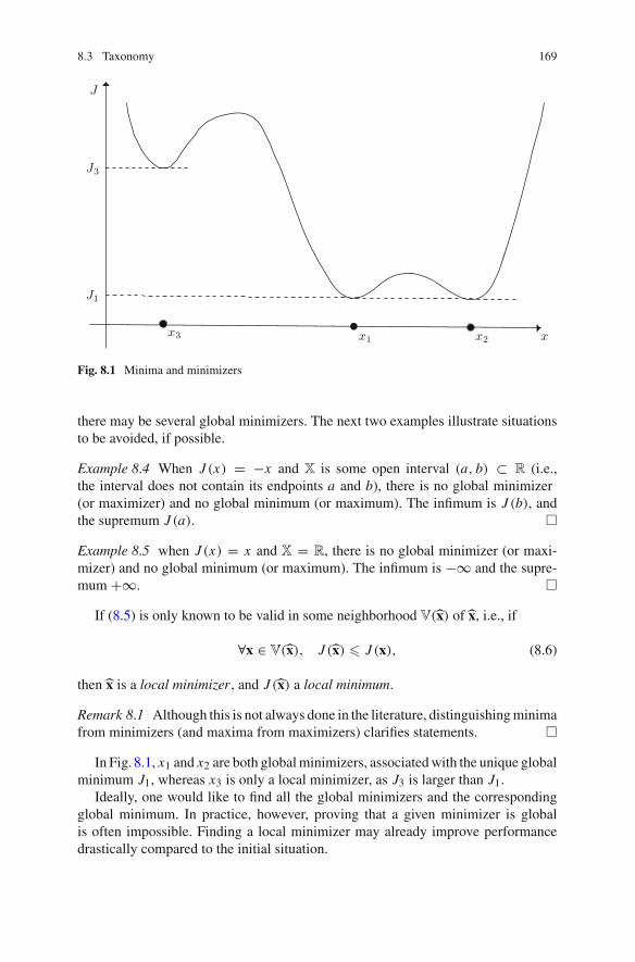
8.3 Taxonomy 169

x1 x2 xx3

J1

J3

J

Fig. 8.1 Minima and minimizers

there may be several global minimizers. The next two examples illustrate situationsto be avoided, if possible.

Example 8.4 When J (x) = −x and X is some open interval (a, b) ⊂ R (i.e.,the interval does not contain its endpoints a and b), there is no global minimizer(or maximizer) and no global minimum (or maximum). The infimum is J (b), andthe supremum J (a). �

Example 8.5 when J (x) = x and X = R, there is no global minimizer (or maxi-mizer) and no global minimum (or maximum). The infimum is −∞ and the supre-mum +∞. �

If (8.5) is only known to be valid in some neighborhood V(x) of x, i.e., if

∀x ∈ V(x), J (x) � J (x), (8.6)

then x is a local minimizer, and J (x) a local minimum.

Remark 8.1 Although this is not always done in the literature, distinguishing minimafrom minimizers (and maxima from maximizers) clarifies statements. �

In Fig. 8.1, x1 and x2 are both global minimizers, associated with the unique globalminimum J1, whereas x3 is only a local minimizer, as J3 is larger than J1.

Ideally, one would like to find all the global minimizers and the correspondingglobal minimum. In practice, however, proving that a given minimizer is globalis often impossible. Finding a local minimizer may already improve performancedrastically compared to the initial situation.

170 8 Introduction to Optimization

Optimization problems may be classified according to the type of their feasibledomain X:

• X = Rn corresponds to unconstrained continuous optimization (Chap. 9).

• X � Rn corresponds to constrained optimization (Chap. 10). The constraints

express that some values of the decision variables are not acceptable (for instance,some variables may have to be positive). We distinguish equality constraints

cej (x) = 0, j = 1, . . . , ne, (8.7)

and inequality constraints

cij (x) � 0, j = 1, . . . , ni. (8.8)

A more concise notation isce(x) = 0 (8.9)

andci(x) � 0, (8.10)

which should be understood as valid componentwise.• When X is finite and the decision variables are not quantitative, one speaks of

combinatorial optimization (Chap. 11).• When X is an infinite-dimensional function space, one speaks of functional opti-

mization, encountered, for instance, in optimal control theory [12] and not con-sidered in this book.

Remark 8.2 Nothing forbids the constraints defining X to involve numericalquantities computed via a model from the numerical values taken by the decisionvariables. In optimal control, for instance, one may require that the state of the dynam-ical system being controlled satisfies some inequality constraints at given instants oftime. �

Remark 8.3 Whenever possible, inequality constraints are written as cij (x) � 0

rather than as cij (x) < 0, to allow X to be a closed set (i.e., a set that contains its

boundary). When cij (x) = 0, the j th inequality constraint is said to be saturated (or

active). �

Remark 8.4 When X is such that some entries xi of the decision vector x can onlytake integer values and these values have some quantitative meaning, one may preferto speak of integer programming rather than of combinatorial programming, althoughthe two are sometimes used interchangeably. A problem of integer programming maybe converted into one of constrained continuous optimization. If, for instance, X issuch that xi ∈ {0, 1, 2, 3}, then one may enforce the constraint

8.3 Taxonomy 171

xi (1 − xi )(2 − xi )(3 − xi ) = 0. (8.11)

�

Remark 8.5 The number n = dim x of decision variables has a strong influence onthe complexity of the optimization problem and on the methods that can be used,because of what is known as the curse of dimensionality. A method that would beperfectly viable for n = 2 may fail hopelessly for n = 50, as illustrated by the nextexample. �

Example 8.6 Let X be an n-dimensional unit hypercube [0, 1]×· · ·×[0, 1]. Assumethat minimization is by random search, with xk (k = 1, . . . , N ) picked at random inX according to a uniform distribution and the decision vector xk achieving the lowestcost so far taken as an estimate of a global minimizer. The width of a hypercube H

that has a probability p of being hit is ∂ = p1/n , and this width increases veryquickly with n. For p = 10−3, for instance, ∂ = 10−3 if n = 1, ∂ ≈ 0.5 if n = 10and ∂ ≈ 0.87 if n = 50. When n increases, it thus soon becomes impossible toexplore any small region of decision space. To put it in another way, if 100 pointsare deemed appropriate for sampling the interval [0, 1], then 100n samples must bedrawn in X to achieve a similar density. Fortunately, the regions of actual interestin high-dimensional decision spaces often correspond to lower dimensional hypersurfaces than may still be explored efficiently provided that more sophisticated searchmethods are used. �

The type of the cost function also has a strong influence on the type of method tobe employed.

• When J (x) is linear in x, it can be written as

J (x) = cTx. (8.12)

One must then introduce constraints to avoid x tending to infinity in the direction−c, which would in general be meaningless. If the contraints are linear (or affine)in x, then the problem pertains to linear programming (see Sect. 10.6).

• If J (x) is quadratic in x and can be written as

J (x) = [Ax − b]TQ[Ax − b], (8.13)

where A is a known matrix such that ATA is invertible, Q is a known symmetricpositive definite weighting matrix and b is a known vector, and if X = R

n , thenlinear least squares can be used to evaluate the unique global minimizer of thecost (see Sect. 9.2).

• When J (x) is nonlinear in x (without being quadratic), two cases have to bedistinguished.

172 8 Introduction to Optimization

– If J (x) is differentiable, for instance when minimizing

J (x) =N∑

i=1

[ei (x)]2, (8.14)

with ei (x) differentiable, then one may employ Taylor expansions of the costfunction, which leads to the gradient and Newton methods and their variants(see Sect. 9.3.4).

– If J (x) is not differentiable, for instance when minimizing

J (x) =∑

i

|ei (x)|, (8.15)

orJ (x) = max

ve(x, v), (8.16)

then specific methods are necessary (see Sects. 9.3.5, 9.4.1.2 and 9.4.2.1). Evensuch an innocent-looking cost function as (8.15), which is differentiable almosteverywhere if the ei (x)’s are differentiable, cannot be minimized by an iterativeoptimization method based on a limited expansion of the cost, as this methodwill usually hurl itself onto a point where the cost is not differentiable to staystuck there.

• When J (x) is convex on X, the powerful methods of convex optimization can beemployed, provided that X is also convex. See Sect. 10.7.

Remark 8.6 The time needed for a single evaluation of J (x) also has consequenceson the types of methods that can be employed. When each evaluation takes a fractionof a second, random search and evolutionary algorithms may be viable options. Thisis no longer the case when each evaluation takes several hours, for instance because itinvolves the simulation of a complex knowledge-based model, as the computationalbudget is then severely restricted, see Sect. 9.4.3. �

8.4 How About a Free Lunch?

In the context of optimization, a free lunch would be a universal method, ableefficiently to treat any optimization problem, thus eliminating the need to adapt tothe specifics of the problem at hand. It could have been the Holy Grail of evolutionaryoptimization, had not Wolpert and Macready published their no free lunch (NFL)theorems.

8.4 How About a Free Lunch? 173

8.4.1 There Is No Such Thing

The NFL theorems in [13] (see also [14]) assume that

1. an oracle is available, which returns the numerical value of J (x) when given anynumerical value of x ∈ X,

2. the search space X is finite,3. the cost function J (·) can only take finitely many numerical values,4. nothing else is known about J (·) a priori,5. the competing algorithms Ai are deterministic,6. the (finitely many) minimization problems M j that can be generated under

Hypotheses 2 and 3 all have the same probability,7. the performance PN (Ai ,M j ) of the algorithm Ai on the minimization problem

M j for N distinct and time-ordered visited points xk ∈ X is only a function ofthe values taken by xk and J (xk), k = 1, . . . , N .

Hypotheses 2 and 3 are always met when computing with floating-point numbers.Assume, for instance, that 64-bit double floats are used. Then

• the number representing J (x) cannot take more than 264 values,• the representation of X cannot have more than (264)dim x elements, with dim x the

number of decision variables.

An upper bound of the number �M of minimization problems is thus (264)dim x+1.Hypothesis 4 makes it impossible to take advantage of any additional knowledge

about the minimization problem to be solved, which cannot be assumed to be convex,for instance.

Hypothesis 5 is met by all the usual black-box minimization methods such assimulated annealing or evolutionary algorithms, even if they seem to incorporaterandomness, as any pseudorandom number generator is deterministic for a givenseed.

The performance measure might be, e.g., the best value of the cost obtained so far

PN (Ai ,M j ) = Nmink=1

J (xk). (8.17)

Note that the time needed by a given algorithm to visit N distinct points in X cannotbe taken into account in the performance measure.

We only consider the first of the NFL theorems in [13], which can be summarizedas follows: for any pair of algorithms (A1,A2), the mean performance over allminimization problems is the same, i.e.,

1

�M

�M∑

j=1

PN (A1,M j ) = 1

�M

�M∑

j=1

PN (A2,M j ). (8.18)

174 8 Introduction to Optimization

In other words, if A1 performs better on average than A2 for a given class ofminimization problems, then A2 must perform better on average than A1 on all theothers...

Example 8.7 Let A1 be a hill-descending algorithm, which moves from xk to xk+1

by selecting, among its neighbors in X, one of those with the lowest cost. Let A2be a hill-ascending algorithm, which selects one of the neighbors with the highestcost instead, and let A3 pick xk at random in X. Measure performance by the lowestcost achieved after exploring N distinct points in X. The average performance ofthese three algorithms is the same. In other words, the algorithm does not matteron average, and showing that A1 performs better than A2 or A3 on a few test casescannot disprove this disturbing fact. �

8.4.2 You May Still Get a Pretty Inexpensive Meal

The NFL theorems tell us that no algorithm can claim to be better than the others interms of averaged performance over all types of problems. Worse, it can be provedvia complexity arguments that global optimization cannot be achieved in the mostgeneral case [7].

It should be noted, however, that most of the �M minimization problems on whichmean performance is computed by (8.18) have no interest from the point of viewof applications. We usually deal with specific classes of minimization problems, forwhich some algorithms are indeed superior to others. When the class of minimizationproblems to be considered is restricted, even slightly, some evolutionary algorithmsmay perform better than others, as demonstrated in [15] on a toy example. Furtherrestrictions, such as requesting that J (·) be convex, may be considered more costlybut allow much more powerful algorithms to be employed.

Unconstrained continuous optimization will be considered first, in Chap. 9.

8.5 In Summary

• Before attempting optimization, check that this does make sense for the actualproblem of interest.

• It is always possible to transform a maximization problem into a minimizationproblem, so considering only minimization is not restrictive.

• The distinction between minima and minimizers is useful to keep in mind.• Optimization problems can be classified according to the type of the feasible

domain X for their decision variables.• The type of the cost function has a strong influence on the classes of methods that

can be used. Non-differentiable cost functions cannot be minimized using methodsbased on a Taylor expansion of the cost.

8.5 In Summary 175

• The dimension of the decision vector is a key factor to be taken into account inthe choice of an algorithm, because of the curse of dimensionality.

• The time required to carry out a single evaluation of the cost function should alsobe taken into consideration.

• There is no free lunch.

References

1. Polyak, B.: Introduction to Optimization. Optimization Software, New York (1987)2. Minoux, M.: Mathematical Programming—Theory and Algorithms. Wiley, New York (1986)3. Gill, P., Murray, W., Wright, M.: Practical Optimization. Elsevier, London (1986)4. Kelley, C.: Iterative Methods for Optimization. SIAM, Philadelphia (1999)5. Nocedal, J., Wright, S.: Numerical Optimization. Springer, New York (1999)6. Bertsekas, D.: Nonlinear Programming. Athena Scientific, Belmont (1999)7. Nesterov, Y.: Introductory Lectures on Convex Optimization: A Basic Course. Kluwer, Boston

(2004)8. Bonnans, J., Gilbert, J.C., Lemaréchal, C., Sagastizabal, C.: Numerical Optimization—

Theoretical and Practical Aspects. Springer, Berlin (2006)9. Ben-Tal, A., El Ghaoui, L., Nemirovski, A.: Robust Optimization. Princeton University Press,

Princeton (2009)10. Watson, L., Bartholomew-Biggs, M., Ford, J. (eds.): Optimization and nonlinear equations.

J. Comput. Appl. Math. 124(1–2):1–373 (2000)11. Floudas, C., Pardalos, P. (eds.): Encyclopedia of Optimization, 2nd edn. Springer, New York

(2009)12. Dorato, P., Abdallah, C., Cerone, V.: Linear-Quadratic Control. An Introduction. Prentice-

Hall, Englewood Cliffs (1995)13. Wolpert, D., Macready, W.: No free lunch theorems for optimization. IEEE Trans. Evol.

Comput. 1(1), 67–82 (1997)14. Ho, Y.C., Pepyne, D.: Simple explanation of the no free lunch theorem of optimization. In:

Proceedings of 40th IEEE Conference on Decision and Control, pp. 4409–4414. Orlando(2001)

15. Droste, S., Jansen, T., Wegener, I.: Perhaps not a free lunch but at least a free appetizer. In:Proceedings of 1st Genetic and Evolutionary Computation Conference, pp. 833–839. Orlando(1999)

Chapter 9Optimizing Without Constraint

In this chapter, the decision vector x is just assumed to belong to Rn . There is no

equality constraint, and inequality constraints, if any, are assumed not to be saturatedat any minimizer, so they might as well not exist (except possibly to make sure thatthe decision vector does not wander temporarily into uncharted territories).

9.1 Theoretical Optimality Conditions

The optimality conditions presented here have inspired useful algorithms and stop-ping conditions. Assume that the cost function J (·) is differentiable, and write downits first-order Taylor expansion around a minimizer x

J (x + ∂x) = J (x) +n⎡

i=1

∂ J

∂xi(x)∂xi + o(||∂x||), (9.1)

or, more concisely,

J (x + ∂x) = J (x) + gT(x)∂x + o(||∂x||), (9.2)

with g(x) the gradient of the cost function evaluated at x

g(x) = ∂ J

∂x(x) =

⎢

⎣⎣⎣⎣⎣⎣⎣⎤

∂ J∂x1

∂ J∂x2...

∂ J∂xn

⎥

⎦⎦⎦⎦⎦⎦⎦⎞

(x). (9.3)

É. Walter, Numerical Methods and Optimization, 177DOI: 10.1007/978-3-319-07671-3_9,© Springer International Publishing Switzerland 2014

178 9 Optimizing Without Constraint

x

J(x)

x

Fig. 9.1 The stationary point x is a maximizer

Example 9.1 Topographical analogyIf J (x) is the altitude at x, with x1 the longitude and x2 the latitude, then g(x) is

the direction of steepest ascent, i.e., the direction along which altitude increases themost quickly when leaving x. �

For x to be a minimizer of J (·) (at least locally), the first-order term in ∂x shouldnever contribute to decreasing the cost, so it must satisfy

gT(x)∂x � 0 √∂x ∇ Rn . (9.4)

Since (9.4) must still be satisfied if ∂x is replaced by −∂x,

gT(x)∂x = 0 √∂x ∇ Rn . (9.5)

Because there is no constraint on ∂x, this is possible only if the gradient of the costat x is zero. A necessary first-order optimality condition is thus

g(x) = 0. (9.6)

This stationarity condition does not suffice to guarantee that x is a minimizer, evenlocally. It may just as well be a local maximizer (Fig. 9.1) or a saddle point, i.e., apoint from which the cost increases in some directions and decreases in others. If adifferentiable cost function has no stationary point, then the associated optimizationproblem is meaningless in the absence of constraint.

9.1 Theoretical Optimality Conditions 179

Consider now the second-order Taylor expansion of the cost function around x

J (x + ∂x) = J (x) + gT(x)∂x + 1

2

n⎡

i=1

n⎡

j=1

∂2 J

∂xi∂x j(x)∂xi∂x j + o(||∂x||2), (9.7)

or, more concisely,

J (x + ∂x) = J (x) + gT(x)∂x + 1

2∂xTH(x)∂x + o(||∂x||2). (9.8)

H(x) is the Hessian of the cost function evaluated at x

H(x) = ∂2 J

∂x∂xT (x). (9.9)

It is a symmetric matrix, such that its entry in position (i, j) satisfies

hi, j (x) = ∂2 J

∂xi∂x j(x). (9.10)

If the necessary first-order optimality condition (9.6) is satisfied, then

J (x + ∂x) = J (x) + 1

2∂xTH(x)∂x + o(||∂x||2), (9.11)

and the second-order term in ∂x should never contribute to decreasing the cost. Anecessary second-order optimality condition is therefore

∂xTH(x)∂x � 0 √∂x, (9.12)

so all the eigenvalues of H(x) must be positive or zero. This amounts to saying thatH(x) must be symmetric non-negative definite, which is denoted by

H(x) � 0. (9.13)

Together, (9.6) and (9.13) do not make a sufficient condition for optimality, evenlocally, as zero eigenvalues of H(x) are associated with eigenvectors along which itis possible to move away from x without increasing the contribution of the second-order term to the cost. It would then be necessary to consider higher order terms toreach a conclusion. To prove, for instance, that J (x) = x1000 has a local minimizerat x = 0 via a Taylor-series expansion, one would have to compute all the derivativesof this cost function up to order 1000, as all lower order derivatives take the valuezero at x .

180 9 Optimizing Without Constraint

The more restrictive condition

∂xTH(x)∂x > 0 √∂x, (9.14)

which forces all the eigenvalues of H(x) to be strictly positive, yields a sufficientsecond-order local optimality condition (provided that the necessary first-order opti-mality condition (9.6) is also satisfied). It is equivalent to saying that H(x) is sym-metric positive definite, which is denoted by

H(x) → 0. (9.15)

In summary, a necessary condition for the optimality of x is

g(x) = 0 and H(x) � 0, (9.16)

and a sufficient condition for the local optimality of x is

g(x) = 0 and H(x) → 0. (9.17)

Remark 9.1 There is, in general, no necessary and sufficient local optimality condi-tion. �

Remark 9.2 When nothing else is known about the cost function, satisfaction of(9.17) does not guarantee that x is a global minimizer. �

Remark 9.3 The conditions on the Hessian are valid only for a minimization. For amaximization, � should be replaced by �, and → by ⇒. �

Remark 9.4 As (9.6) suggests, methods for solving systems of equations seen inChaps. 3 (for linear systems) and 7 (for nonlinear systems) can also be used to lookfor minimizers. Advantage can then be taken of the specific properties of the Jacobianmatrix of the gradient (i.e., the Hessian), which (9.13) tells us should be symmetricnon-negative definite at any local or global minimizer. �

Example 9.2 Kriging revisitedEquations (5.61) and (5.64) of the Kriging predictor can be derived via the the-

oretical optimality conditions (9.6) and (9.15). Assume, as in Sect. 5.4.3, that Nmeasurements have taken place, to get

yi = f (xi ), i = 1, . . . , N . (9.18)

In its simplest version, Kriging interprets these results as realizations of a zero-meanGaussian process (GP) Y (x). Then

√x, E{Y (x)} = 0 (9.19)

9.1 Theoretical Optimality Conditions 181

and√xi ,√x j , E{Y (xi )Y (x j )} = σ2

yr(xi , x j ), (9.20)

with r(·, ·) a correlation function, such that r(x, x) = 1, and with σ2y the GP variance.

Let Y (x) be a linear combination of the Y (xi )’s, i.e.,

Y (x) = cT(x)Y, (9.21)

where Y is the random vector

Y = [Y (x1), Y (x2), . . . , Y (xN )]T (9.22)

and c(x) is a vector of weights. Y (x) is an unbiased predictor of Y (x), as for all x

E{Y (x) − Y (x)} = E{Y (x)} − E{Y (x)} = cT(x)E{Y} = 0. (9.23)

There is thus no systematic error for any vector of weights c(x). The best linearunbiased predictor (or BLUP) of Y (x) sets c(x) so as to minimize the variance ofthe prediction error at x. Now

[Y (x) − Y (x)]2 = cT(x)YYTc(x) + [Y (x)]2 − 2cT(x)YY (x). (9.24)

The variance of the prediction error is thus

E{[Y (x) − Y (x)]2} = cT(x)E⎠

YYT}

c(x) + σ2y − 2cT(x)E{YY (x)}

= σ2y

[cT(x)Rc(x) + 1 − 2cT(x)r(x)

], (9.25)

with R and r(x) defined by (5.62) and (5.63). Minimizing this variance with respectto c is thus equivalent to minimizing

J (c) = cTRc + 1 − 2cTr(x). (9.26)

The first-order condition for optimality (9.6) translates into

∂ J

∂c(c) = 2Rc − 2r(x) = 0. (9.27)

Provided that R is invertible, as it should, (9.27) implies that the optimal weightingvector is

c(x) = R−1r(x). (9.28)

182 9 Optimizing Without Constraint

Since R is symmetric, (9.21) and (9.28) imply that

Y (x) = rT(x)R−1Y. (9.29)

The predicted mean based on the data y is thus

y(x) = rT(x)R−1y, (9.30)

which is (5.61). Replace c(x) by its optimal value c(x) in (9.25) to get the (optimal)prediction variance

σ2(x) = σ2y

[rT(x)R−1RR−1r(x) + 1 − 2rT(x)R−1r(x)

]

= σ2y

[1 − rT(x)R−1r(x)

], (9.31)

which is (5.64).Condition (9.17) is satisfied, provided that

∂2 J

∂c∂cT (c) = 2R → 0. (9.32)

�

Remark 9.5 Example 9.2 neglects the fact that σ2y is unknown and that the correlation

function r(xi , x j ) often involves a vector p of parameters to be estimated from thedata, so R and r(x) should actually be written R(p) and r(x, p). The most commonapproach for estimating p and σ2

y is maximum likelihood. The probability density ofthe data vector y is then maximized under the hypothesis that it was generated bya model with parameters p and σ2

y . The maximum-likelihood estimates of p and σ2y

are thus obtained by solving yet another optimization problem, as

p = arg minp

[N ln

(yTR−1(p)y

N

)+ ln det R(p)

](9.33)

and

σ2y = yTR−1(p)y

N. (9.34)

Replacing R by R(p), r(x) by r(x, p) and σ2y by σ2

y in (5.61) and (5.64), one gets anempirical BLUP, or EBLUP [1]. �

9.2 Linear Least Squares 183

9.2 Linear Least Squares

Linear least squares [2, 3] are another direct application of the theoretical optimalityconditions (9.6) and (9.15) to an important special case where they yield a closed-form optimal solution. This is when the cost function is quadratic in the decisionvector x. (Example 9.2 already illustrated this special case, with c the decision vector.)The cost function is now assumed quadratic in an error that is affine in x.

9.2.1 Quadratic Cost in the Error

Let y be a vector of numerical data, and f(x) be the output of some model of thesedata, with x a vector of model parameters (the decision variables) to be estimated.In general, there are more data than parameters, so

N = dim y = dim f(x) > n = dim x. (9.35)

As a result, there is usually no solution for x of the system of equations

y = f(x). (9.36)

The interpolation of the data should then be replaced by their approximation. Definethe error as the vector of residuals

e(x) = y − f(x). (9.37)

The most commonly used strategy for estimating x from the data is to minimize acost function that is quadratic in e(x), such as

J (x) = eT(x)We(x), (9.38)

where W → 0 is some known weighting matrix, chosen by the user. The weightedleast squares estimate of x is then

x = arg minx∇Rn

[y − f(x)]TW[y − f(x)]. (9.39)

One can always compute, for instance with the Cholesky method of Sect. 3.8.1, amatrix M such that

W = MTM, (9.40)

sox = arg min

x∇Rn[My − Mf(x)]T[My − Mf(x)]. (9.41)

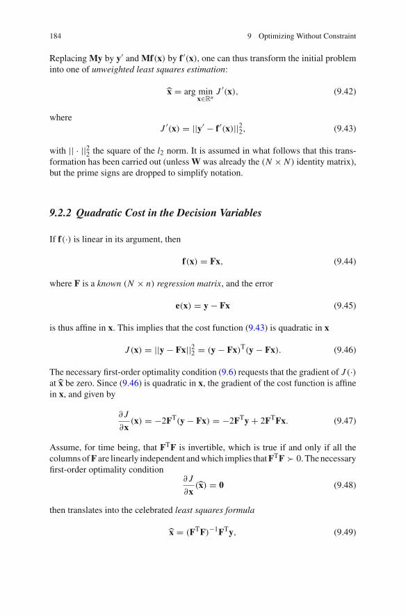
184 9 Optimizing Without Constraint

Replacing My by y∈ and Mf(x) by f ∈(x), one can thus transform the initial probleminto one of unweighted least squares estimation:

x = arg minx∇Rn

J ∈(x), (9.42)

whereJ ∈(x) = ||y∈ − f ∈(x)||22, (9.43)

with || · ||22 the square of the l2 norm. It is assumed in what follows that this trans-formation has been carried out (unless W was already the (N × N ) identity matrix),but the prime signs are dropped to simplify notation.

9.2.2 Quadratic Cost in the Decision Variables

If f(·) is linear in its argument, then

f(x) = Fx, (9.44)

where F is a known (N × n) regression matrix, and the error

e(x) = y − Fx (9.45)

is thus affine in x. This implies that the cost function (9.43) is quadratic in x

J (x) = ||y − Fx||22 = (y − Fx)T(y − Fx). (9.46)

The necessary first-order optimality condition (9.6) requests that the gradient of J (·)at x be zero. Since (9.46) is quadratic in x, the gradient of the cost function is affinein x, and given by

∂ J

∂x(x) = −2FT(y − Fx) = −2FTy + 2FTFx. (9.47)

Assume, for time being, that FTF is invertible, which is true if and only if all thecolumns of F are linearly independent and which implies that FTF → 0. The necessaryfirst-order optimality condition

∂ J

∂x(x) = 0 (9.48)

then translates into the celebrated least squares formula

x = (FTF)−1FTy, (9.49)

9.2 Linear Least Squares 185

which is a closed-form expression for the unique stationary point of the cost function.Moreover, since FTF → 0, the sufficient condition for local optimality (9.17) issatisfied and (9.49) is a closed-form expression for the unique global minimizer ofthe cost function. This is a considerable advantage over the general case where no suchclosed-form solution exists. See Sect. 16.8 for a beautiful example of a systematic andrepetitive use of linear least squares in the context of building nonlinear black-boxmodels.

Example 9.3 Polynomial regressionLet yi be the value measured for some quantity of interest at the known instant

of time ti (i = 1, . . . , N ). Assume that these data are to be approximated with a kthorder polynomial in the power series form

Pk(t, x) =k⎡

i=0

pi ti , (9.50)

wherex = (p0 p1 . . . pk)

T. (9.51)

Assume also that there are more data than parameters (N > n = k +1). To computethe estimate x of the parameter vector x, one may look for the value of x that minimizes

J (x) =N⎡

i=1

[yi − Pk(ti , x)]2 = ||y − Fx||22, (9.52)

withy = [y1 y2 . . . yN ]T (9.53)

and

F =

⎢

⎣⎣⎣⎣⎣⎣⎤

1 t1 t21 · · · tk

11 t2 t2

2 · · · tk2

......

......

......

......

1 tN t2N · · · tk

N

⎥

⎦⎦⎦⎦⎦⎦⎞. (9.54)

Mathematically, the optimal solution is then given by (9.49). �

Remark 9.6 The key point in Example 9.3 is that the model output Pk(t, x) is linearin x. Thus, for instance, the function

f (t, x) = x1e−t + x2t2 + x3

t(9.55)

could benefit from a similar treatment. �

186 9 Optimizing Without Constraint

Despite its elegant conciseness, (9.49) should seldom be used for computingleast squares estimates, for at least two reasons.

First, inverting FTF usually requires unnecessary computations and it is less workto solve the system of linear equations

FTFx = FTy, (9.56)

which are called the normal equations. Since FTF is assumed, for the time being, tobe positive definite, one may use Cholesky factorization for this purpose. This is themost economical approach, only applicable to well-conditioned problems.

Second, the condition number of FTF is almost always considerably worse thanthat of F, as will be explained in Sect. 9.2.4. This suggests the use of methods suchas those presented in the next two sections, which avoid computing FTF.

Sometimes, however, FTF takes a particularly simple diagonal form. This maybe due to experiment design, as in Example 9.4, or to a proper choice of the modelrepresentation, as in Example 9.5. Solving (9.56) then becomes trivial, and there isno reason for avoiding it.

Example 9.4 Factorial experiment design for a quadratic modelAssume that some quantity of interest y(u) is modeled as

ym(u, x) = p0 + p1u1 + p2u2 + p3u1u2, (9.57)

where u1 and u2 are input factors, the value of which can be chosen freely in thenormalized interval [−1, 1] and where

x = (p0, . . . , p3)T. (9.58)

The parameters p1 and p2 respectively quantify the effects of u1 and u2 alone, whilep3 quantifies the effect of their interaction. Note that there is no term in u2

1 or u22. The

parameter vector x is to be estimated from the experimental data y(ui ), i = 1, . . . , N ,by minimizing

J (x) =N⎡

i=1

[y(ui ) − ym(ui , x)

]2. (9.59)

A two-level full factorial design consists of collecting data at all possible combi-nations of the two extreme possible values {−1, 1} of the factors, as in Table 9.1,and this pattern may be repeated to decrease the influence of measurement noise.Assume it is repeated once, so N = 8. The entries of the resulting (8 × 4) regressionmatrix F are then those of Table 9.2, deprived of its first row and first column.

9.2 Linear Least Squares 187

Table 9.1 Two-level full factorial experiment design

Experiment number Value of u1 Value of u2

1 −1 −12 −1 13 1 −14 1 1

Table 9.2 Building F

Experiment number Constant Value of u1 Value of u2 Value of u1u2

1 1 −1 −1 12 1 −1 1 −13 1 1 −1 −14 1 1 1 15 1 −1 −1 16 1 −1 1 −17 1 1 −1 −18 1 1 1 1

It is trivial to check thatFTF = 8I4, (9.60)

so cond(FTF) = 1, and (9.56) implies that

x = 1

8FTy. (9.61)

This example generalizes to any number of input factors, provided that the quadraticpolynomial model contains no quadratic term in any of the input factors alone.Otherwise, the column of F associated with any such term would consist of ones andthus be identical to the column of F associated with the constant term. As a result,FTF would no longer be invertible. Three-level factorial designs may be used in thiscase. �

Example 9.5 Least squares approximation of a function over [−1, 1]We look for the polynomial (9.50) that best approximates a function f (·) over the

normalized interval [−1, 1] in the sense that

J (x) =1∫

−1

[ f (δ ) − Pk(δ, x)]2dδ (9.62)

is minimized. The optimal value x of the parameter vector x of the polynomialsatisfies a continuous counterpart of the normal equations

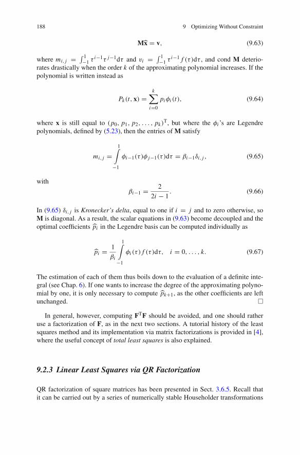
188 9 Optimizing Without Constraint

Mx = v, (9.63)

where mi, j = ∫ 1−1 δ i−1δ j−1dδ and vi = ∫ 1

−1 δ i−1 f (δ )dδ , and cond M deterio-rates drastically when the order k of the approximating polynomial increases. If thepolynomial is written instead as

Pk(t, x) =k⎡

i=0

piαi (t), (9.64)

where x is still equal to (p0, p1, p2, . . . , pk)T, but where the αi ’s are Legendre

polynomials, defined by (5.23), then the entries of M satisfy

mi, j =1∫

−1

αi−1(δ )α j−1(δ )dδ = ρi−1∂i, j , (9.65)

with

ρi−1 = 2

2i − 1. (9.66)

In (9.65) ∂i, j is Kronecker’s delta, equal to one if i = j and to zero otherwise, soM is diagonal. As a result, the scalar equations in (9.63) become decoupled and theoptimal coefficients pi in the Legendre basis can be computed individually as

pi = 1

ρi

1∫

−1

αi (δ ) f (δ )dδ, i = 0, . . . , k. (9.67)

The estimation of each of them thus boils down to the evaluation of a definite inte-gral (see Chap. 6). If one wants to increase the degree of the approximating polyno-mial by one, it is only necessary to compute pk+1, as the other coefficients are leftunchanged. �

In general, however, computing FTF should be avoided, and one should ratheruse a factorization of F, as in the next two sections. A tutorial history of the leastsquares method and its implementation via matrix factorizations is provided in [4],where the useful concept of total least squares is also explained.

9.2.3 Linear Least Squares via QR Factorization

QR factorization of square matrices has been presented in Sect. 3.6.5. Recall thatit can be carried out by a series of numerically stable Householder transformations

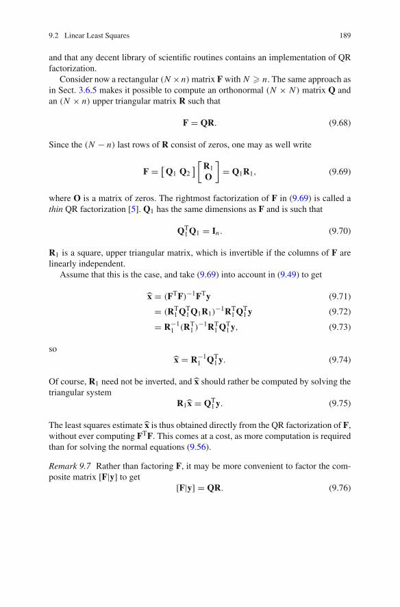
9.2 Linear Least Squares 189

and that any decent library of scientific routines contains an implementation of QRfactorization.

Consider now a rectangular (N ×n) matrix F with N � n. The same approach asin Sect. 3.6.5 makes it possible to compute an orthonormal (N × N ) matrix Q andan (N × n) upper triangular matrix R such that

F = QR. (9.68)

Since the (N − n) last rows of R consist of zeros, one may as well write

F = [Q1 Q2

] [R1O

]= Q1R1, (9.69)

where O is a matrix of zeros. The rightmost factorization of F in (9.69) is called athin QR factorization [5]. Q1 has the same dimensions as F and is such that

QT1 Q1 = In . (9.70)

R1 is a square, upper triangular matrix, which is invertible if the columns of F arelinearly independent.

Assume that this is the case, and take (9.69) into account in (9.49) to get

x = (FTF)−1FTy (9.71)

= (RT1 QT

1 Q1R1)−1RT

1 QT1 y (9.72)

= R−11 (RT

1 )−1RT1 QT

1 y, (9.73)

sox = R−1

1 QT1 y. (9.74)

Of course, R1 need not be inverted, and x should rather be computed by solving thetriangular system

R1x = QT1 y. (9.75)

The least squares estimate x is thus obtained directly from the QR factorization of F,without ever computing FTF. This comes at a cost, as more computation is requiredthan for solving the normal equations (9.56).

Remark 9.7 Rather than factoring F, it may be more convenient to factor the com-posite matrix [F|y] to get

[F|y] = QR. (9.76)

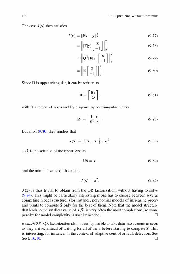
190 9 Optimizing Without Constraint

The cost J (x) then satisfies

J (x) = ‖Fx − y‖22 (9.77)

=∥∥∥∥[F|y]

[x

−1

]∥∥∥∥2

2(9.78)

=∥∥∥∥QT[F|y]

[x

−1

]∥∥∥∥2

2(9.79)

=∥∥∥∥R

[x

−1

]∥∥∥∥2

2. (9.80)

Since R is upper triangular, it can be written as

R =[

R1O

], (9.81)

with O a matrix of zeros and R1 a square, upper triangular matrix

R1 =[

U v0T σ

]. (9.82)

Equation (9.80) then implies that

J (x) = ‖Ux − v‖22 + σ2, (9.83)

so x is the solution of the linear system

Ux = v, (9.84)

and the minimal value of the cost is

J (x) = σ2. (9.85)

J (x) is thus trivial to obtain from the QR factorization, without having to solve(9.84). This might be particularly interesting if one has to choose between severalcompeting model structures (for instance, polynomial models of increasing order)and wants to compute x only for the best of them. Note that the model structurethat leads to the smallest value of J (x) is very often the most complex one, so somepenalty for model complexity is usually needed. �

Remark 9.8 QR factorization also makes it possible to take data into account as soonas they arrive, instead of waiting for all of them before starting to compute x. Thisis interesting, for instance, in the context of adaptive control or fault detection. SeeSect. 16.10. �

9.2 Linear Least Squares 191

9.2.4 Linear Least Squares via Singular Value Decomposition

Singular value decomposition (or SVD) requires even more computation than QRfactorization but may facilitate the treatment of problems where the columns of Fare linearly dependent or nearly linearly dependent, see Sects. 9.2.5 and 9.2.6.

Any (N × n) matrix F with N � n can be factored as

F = UλVT, (9.86)

where

• U has the same dimensions as F, and is such that

UTU = In, (9.87)

• λ is a diagonal (n × n) matrix, the diagonal entries σi of which are the singularvalues of F, with σi � 0,

• V is an (n × n) matrix such that

VTV = In . (9.88)

Equation (9.86) implies that

FV = Uλ, (9.89)

FTU = Vλ. (9.90)

In other words,

Fvi = σi ui , (9.91)

FTui = σi vi , (9.92)

where vi is the i th column of V and ui the i th column of U. This is why vi and ui

are called right and left singular vectors, respectively.

Remark 9.9 While (9.88) implies that

V−1 = VT, (9.93)

(9.87) gives no magic trick for inverting U, which is not square! �

The computation of the SVD (9.86) is classically carried out in two steps [6],[7]. During the first of them, orthonormal matrices P1 and Q1 are computed so as toensure that

B = PT1 FQ1 (9.94)

192 9 Optimizing Without Constraint

is bidiagonal (i.e., it has nonzero entries only in its main descending diagonal and thedescending diagonal immediately above), and that its last (N − n) rows consist ofzeros. Left- or right-multiplication of a matrix by an orthonormal matrix preservesits singular values, so the singular values of B are the same as those of F. The compu-tation of P1 and Q1 is achieved through two series of Householder transformations.The dimensions of B are the same as those of F, but since the last (N − n) rows ofB consist of zeros, the (N × n) matrix P1 with the first n columns of P1 is formed toget a more economical representation

B = PT1 FQ1, (9.95)

where B is square, bidiagonal and consists of the first n rows of B.During the second step, orthonormal matrices P2 and Q2 are computed so as to

ensure thatλ = PT

2 BQ2 (9.96)

is a diagonal matrix. This is achieved by a variant of the QR algorithm presented inSect. 4.3.6. Globally,

λ = PT2 PT

1 FQ1Q2, (9.97)

and (9.86) is satisfied, with U = P1P2 and VT = QT2 QT

1 .The reader is invited to consult [8] for more detail about modern methods to com-

pute SVDs, and [9] to get an idea of how much effort has been devoted to improvingefficiency and robustness. Routines for computing SVDs are widely available, andone should carefully refrain from any do-it-yourself attempt.

Remark 9.10 SVD has many applications besides the evaluation of linear leastsquares estimates in a numerically robust way. A few of its important propertiesare as follows:

• the column rank of F and the rank of FTF are equal to the number of nonzerosingular values of F, so FTF is invertible if and only if all the singular values of Fdiffer from zero;

• the singular values of F are the square roots of the eigenvalues of FTF (this is nothow they are computed in practice, however);

• if the singular values of F are indexed in decreasing order and if σk > 0, then therank-k matrix that is the closest to F in the sense of the spectral norm is

Fk =k⎡

i=1

σi ui vTi , (9.98)

and||F − Fk ||2 = σk+1. (9.99)

�

9.2 Linear Least Squares 193

Still assuming, for the time being, that FTF is invertible, replace F in (9.49) byUλVT to get

x = (VλUTUλVT)−1VλUTy (9.100)

= (Vλ2VT)−1VλUTy (9.101)

= (VT)−1λ−2V−1VλUTy. (9.102)

Since(VT)−1 = V, (9.103)

this is equivalent to writingx = Vλ−1UTy. (9.104)

As with QR factorization, the optimal solution x is thus evaluated without evercomputing FTF. Inverting λ is trivial, as it is diagonal.

Remark 9.11 All of the methods for obtaining x that have just been described aremathematically equivalent, but their numerical properties differ. �

We have seen in Sect. 3.3 that the condition number of a square matrix for thespectral norm is the ratio of its largest singular value to its smallest, and the sameholds true for rectangular matrices such as F. Now

FTF = VλTUTUλVT = Vλ2VT, (9.105)

which is an SVD of FTF. Each singular value of FTF is thus equal to the square ofthe corresponding singular value of F. For the spectral norm, this implies that

cond (FTF) = (cond F)2. (9.106)

Using the normal equations may thus lead to a drastic degradation of the conditionnumber. If, for instance, cond F = 1010, then cond

(FTF

) = 1020 and there is littlehope of obtaining accurate results when solving the normal equations with doublefloats.

Remark 9.12 Evaluating cond F for the spectral norm requires about as much effortas performing an SVD of F, so one may use the value of another condition number todecide whether an SVD is worth computing when in doubt. The MATLAB functioncondest provides a (random) approximate value of the condition number for the1-norm. �

The approaches based on QR factorization and on SVD are both designed notto worsen the condition number of the linear system to be solved. QR factorizationachieves this for less computation than SVD and should thus be the standard work-horse for solving linear least squares problems. We will see on a few examples that

194 9 Optimizing Without Constraint

the solution obtained via QR factorization may actually be slightly more accuratethan the one obtained via SVD. SVD may be preferred when the problem is extremelyill-conditioned, for reasons detailed in the next two sections.

9.2.5 What to Do if FTF Is Not Invertible?

When FTF is not invertible, some columns of F are linearly dependent. As a result,the least squares solution is no longer unique. This should not happen in principle,if the model has been well chosen (after all, it suffices to discard suitable columnsof F and the corresponding parameters to ensure that the remaining columns ofF are linearly independent). This pathological case is nevertheless interesting, asa chemically pure version of a much more common issue, namely the near lineardependency of columns of F, to be considered in Sect. 9.2.6.

Among the nondenumerable infinity of least squares estimates in this degeneratecase, the one with the smallest Euclidean norm is given by

x = Vλ−1UTy, (9.107)

where λ−1 is a diagonal matrix, the i th diagonal entry of which is equal to 1/ σi ifσi ⊂= 0 and to zero otherwise.

Remark 9.13 Contrary to what this notation suggests, λ−1 is singular, of course. �

9.2.6 Regularizing Ill-Conditioned Problems

It frequently happens that the ratio of the extreme singular values of F is very large,which indicates that some columns of F are almost linearly dependent. The conditionnumber of F is then also very large, and that of FTF even worse. As a result, althoughFTF remains mathematically invertible, the least squares estimate x becomes verysensitive to small variations in the data, which makes estimation an ill-conditionedproblem. Among the many regularization approaches available to address this dif-ficulty, a particularly simple one is to force to zero any singular value of F that issmaller than some threshold ∂ to be tuned by the user. This amounts to approximatingF by a matrix with a lower column rank, to which the procedure of Sect. 9.2.5 canthen be applied. The regularized solution is still given by

x = Vλ−1UTy, (9.108)

but the i th diagonal entry of the diagonal matrix λ−1 is now equal to 1/ σi if σi > ∂

and to zero otherwise.

9.2 Linear Least Squares 195

Remark 9.14 When some prior information is available on the possible values of x,a Bayesian approach to regularization might be preferable [10]. If, for instance, theprior distribution of x is assumed to be Gaussian, with known mean x0 and knownvariance �, then the maximum a posteriori estimate xmap of x satisfies the linearsystem

(FTF + �−1)xmap = FTy + �−1x0, (9.109)

and this system should be much better conditioned than the normal equations. �

9.3 Iterative Methods

When the cost function J (·) is not quadratic in its argument, the linear least squaresmethod of Sect. 9.2 does not apply, and one is often led to using iterative methods ofnonlinear optimization, also known as nonlinear programming. Starting from someestimate xk of a minimizer at iteration k, these methods compute xk+1 such that

J (xk+1) � J (xk). (9.110)

Provided that J (x) is bounded from below (as is the case if J (x) is a norm), thisensures that the sequence {J (xk)}∞k=0 converges. Unless the algorithm gets stuck atx0, performance as measured by the cost function will thus have improved.

This raises two important questions that we will leave aside until Sect. 9.3.4.8:

• where to start from (how to choose x0)?• when to stop?

Before quitting linear least squares completely, let us consider a case where they canbe used to decrease the dimension of search space.

9.3.1 Separable Least Squares

Assume that the cost function is still quadratic in the error

J (x) = ‖y − f(x)‖22, (9.111)

and that the decision vector x can be split into p and θθθ, in such a way that

f(x) = F(θθθ)p. (9.112)

The error vectory − F(θθθ)p (9.113)

196 9 Optimizing Without Constraint

is then affine in p. For any given value of θθθ, the corresponding optimal value p(θθθ)

of p can thus be computed by linear least squares, so as to confine nonlinear searchto θθθ space.

Example 9.6 Fitting data with a sum of exponentialsIf the i th data point yi is modeled as

fi (p, θθθ) =m⎡

j=1

p j e−ν j ti , (9.114)

where the measurement time ti is known, then the residual yi − fi (p, θθθ) is affine inp and nonlinear in θθθ. The dimension of search space can thus be halved by usinglinear least squares to compute p(θθθ), a considerable simplification. �

9.3.2 Line Search

Many iterative methods for multivariate optimization define directions along whichline searches are carried out. Because many such line searches may have to takeplace, their aim is modest: they should achieve significant cost decrease with as littlecomputation as possible. Methods for doing so are more sophisticated recipes thanhard science; those briefly presented below are the results of a natural selection thathas left few others.

Remark 9.15 An alternative to first choosing a search direction and then performinga line search along this direction is known as the trust-region method [11]. In thismethod, a quadratic model deemed to be an adequate approximation of the objectivefunction on some trust region is used to choose the direction and size of the displace-ment of the decision vector simultaneously. The trust region is adapted based on thepast performance of the algorithm. �

9.3.2.1 Parabolic Interpolation

Let β be the scalar parameter associated with the search direction d. Its value may bechosen via parabolic interpolation, where a second-order polynomial P2(β) is usedto interpolate

f (β) = J (xk + βd) (9.115)

at βi , i = 1, 2, 3, with β1 < β2 < β3. Lagrange interpolation formula (5.14)translates into

9.3 Iterative Methods 197

P2(β) = (β − β2)(β − β3)

(β1 − β2)(β1 − β3)f (β1)

+ (β − β1)(β − β3)

(β2 − β1)(β2 − β3)f (β2)

+ (β − β1)(β − β2)

(β3 − β1)(β3 − β2)f (β3). (9.116)

Provided that P2(β) is convex and that the points (βi , f (βi )) (i = 1, 2, 3) are notcollinear, P2(β) is minimal at

β = β2 − 1

2

(β2 − β1)2[ f (β2) − f (β3)] − (β2 − β3)

2[ f (β2) − f (β1)](β2 − β1)[ f (β2) − f (β3)] − (β2 − β3)[ f (β2) − f (β1)] , (9.117)

which is then used to compute

xk+1 = xk + βd. (9.118)

Trouble arises when the points (βi , f (βi )) are collinear, as the denominator in (9.117)is then equal to zero, or when P2(β) turns out to be concave, as P2(β) is then maximalat β. This is why more sophisticated line searches are used in practice, such as Brent’smethod.

9.3.2.2 Brent’s Method

Brent’s method [12] is a strategy for safeguarded parabolic interpolation, describedin great detail in [13]. Contrary to Wolfe’s method of Sect. 9.3.2.3, it does not requirethe evaluation of the gradient of the cost and is thus interesting when this gradient iseither unavailable or evaluated by finite differences and thus costly.

The first step is to bracket a (local) minimizer β in some interval [βmin, βmax] bystepping downhill until f (β) starts increasing again. Line search is then restrictedto this interval. When the function f (β) defined by (9.115) is deemed sufficientlycooperative, which means, among other things, that the interpolating polynomialfunction P2(β) is convex and that its minimizer is in [βmin, βmax], (9.117) and (9.118)are used to compute β and then xk+1. In case of trouble, Brent’s method switches toa slower but more robust approach. If the gradient of the cost were available, f (β)

would be easy to compute and one might employ the bisection method of Sect. 7.3.1for solving f (β) = 0. Instead, f (β) is evaluated at two points βk,1 and βk,2, to getsome slope information. These points are located in such a way that, at iteration k,βk,1 and βk,2 are within a fraction σ of the extremities of the current search interval[βk

min, βkmax], where

σ =≈

5 − 1

2≈ 0.618. (9.119)

198 9 Optimizing Without Constraint

Thus

βk,1 = βkmin + (1 − σ)(βk

max − βkmin), (9.120)

βk,2 = βkmin + σ(βk

max − βkmin). (9.121)

If f (βk,1) < f (βk,2), then the subinterval (βk,2, βkmax] is eliminated, which leaves

[βk+1min , βk+1

max] = [βkmin, βk,2], (9.122)

else the subinterval [βkmin, βk,1) is eliminated, which leaves

[βk+1min , βk+1

max] = [βk,1, βkmax]. (9.123)

In both cases, one of the two evaluation points of iteration k remains in the updatedsearch interval, and turns out to be conveniently located within a fraction σ of oneof its extremities. Each iteration but the first thus requires only one additional eval-uation of the cost function, because the other point is one of the two used duringthe previous iteration. This method is called golden-section search, because of therelation between σ and the golden number.

Even if golden-section search makes a thrifty use of cost evaluations, it is muchslower than parabolic interpolation on a good day, and Brent’s algorithm switchesback to (9.117) and (9.118) as soon as the conditions become favorable.

Remark 9.16 When the time needed for evaluating the gradient of the cost function isabout the same as for the cost function itself, one may use, instead of Brent’s method,a safeguarded cubic interpolation where a third-degree polynomial is requested tointerpolate f (β) and to have the same slope at two trial points [14]. Golden sectionsearch can then be replaced by bisection to search for β such that f (β) = 0 whenthe results of cubic interpolation become unacceptable. �

9.3.2.3 Wolfe’s Method

Wolfe’s method [11, 15, 16] carries out an inexact line search, which means thatit only looks for a reasonable value of β instead of an optimal one. Just as inRemark 9.16, Wolfe’s method assumes that the gradient function g(·) can be evalu-ated. It is usually employed for line search in quasi-Newton and conjugate-gradientalgorithms, presented in Sects. 9.3.4.5 and 9.3.4.6.

Two inequalities are used to specify what properties β should satisfy. The first ofthem, known as Armijo condition, states that β should ensure a sufficient decreaseof the cost when moving from xk along the search direction d. It translates into

J (xk+1(β)) � J (xk) + σ1βgT(xk)d, (9.124)

9.3 Iterative Methods 199

where

xk+1(β) = xk + βd (9.125)

and the cost is considered as a function of β. If this function is denoted by f (·), with

f (β) = J (xk + βd), (9.126)

then

f (0) = ∂ J (xk + βd)

∂β(β = 0) = ∂ J

∂xT (xk) · ∂xk+1

∂β= gT(xk)d. (9.127)

So gT(xk)d in (9.124) is the initial slope of the cost function viewed as a function of β.The Armijo condition provides an upper bound on the desirable value of J (xk+1(β)),which is affine in β. Since d is a descent direction, gT(xk)d < 0 and β > 0. Condition(9.124) states that the larger β is, the smaller the cost must become. The internalparameter σ1 should be such that 0 < σ1 < 1, and is usually taken quite small (atypical value is σ1 = 10−4).

The Armijo condition is satisfied for any sufficiently small β, so a bolder strat-egy must be induced. This is the role of the second inequality, known as curvaturecondition, which requests that β also satisfies

f (β) � σ2 f (0), (9.128)

where σ2 ∇ (σ1, 1) (a typical value is σ2 = 0.5). Equation (9.128) translates into

gT(xk + βd)d � σ2gT(xk)d. (9.129)

Since f (0) < 0, any β such that f (β) > 0 will satisfy (9.128). To avoid this, strongWolfe conditions replace the curvature condition (9.129) by

|gT(xk + βd)d| � |σ2gT(xk)d|, (9.130)

while keeping the Armijo condition (9.124) unchanged. With (9.130), f (β) is stillallowed to become positive, but can no longer get too large.

Provided that the cost function J (·) is smooth and bounded below, the existenceof β’s satisfying the Wolfe and strong Wolfe conditions is guaranteed. The principlesof a line search guaranteed to find such a β for strong Wolfe conditions are in [11].Several good software implementations are in the public domain.

200 9 Optimizing Without Constraint

Valley

x1

x2

1

2

3

5

4

6

Fig. 9.2 Bad idea for combining line searches

9.3.3 Combining Line Searches

Once a line-search algorithm is available, it is tempting to deal with multidimensionalsearch by cyclically performing approximate line searches on each component of xin turn. This is a bad idea, however, as search is then confined to displacementsalong the axes of decision space, when other directions might be much more appro-priate. Figure 9.2 shows a situation where altitude is to be minimized with respectto longitude x1 and latitude x2 near some river. The size of the moves soon becomeshopelessly small because no move is allowed along the valley.

A much better approach is Powell’s algorithm, as follows:

1. starting from xk , perform n = dim x successive line searches along linearlyindependent directions di , i = 1, . . . , n, to get xk+ (for the first iteration, thesedirections may correspond to the axes of parameter space, as in cyclic search);

2. perform an additional line search along the average direction of the n previousmoves

d = xk+ − xk (9.131)

to get xk+1;3. replace the best of the di ’s in terms of cost reduction by d, increment k by one

and go to Step 1.

This procedure is shown in Fig. 9.3. While the elimination of the best performerat Step 3 may hurt the reader’s sense of justice, it contributes to maintaining linearindependence among the search directions of Step 1, thereby allowing changes of

9.3 Iterative Methods 201

Valleyx2

x1

xk

xk+d

Fig. 9.3 Powell’s algorithm for combining line searches

direction that may turn out to be needed after a long sequence of nearly collineardisplacements.

9.3.4 Methods Based on a Taylor Expansion of the Cost

Assume now that the cost function is sufficiently differentiable at xk for its first- orsecond-order Taylor expansion around xk to exist. Such an expansion can then beused to decide the next direction along which a line search should be carried out.

Remark 9.17 To establish theoretical optimality conditions in Sect. 9.1, we expandedJ (·) around x, whereas here expansion is around xk . �

9.3.4.1 Gradient Method

The first-order expansion of the cost function around xk satisfies

J (xk + ∂x) = J (xk) + gT(xk)∂x + o(‖∂x‖), (9.132)

so the variation κJ of the cost resulting from the displacement ∂x is such that

κJ = gT(xk)∂x + o(‖∂x‖). (9.133)

202 9 Optimizing Without Constraint

When ∂x is small enough for higher order terms to be negligible, (9.133) suggeststaking ∂x collinear with the gradient at xk and in the opposite direction

∂x = −βkg(xk), with βk > 0. (9.134)

This yields the gradient method

xk+1 = xk − βkg(xk), with βk > 0. (9.135)

If J (x) were an altitude, then the gradient would point in the direction of steepestascent. This explains why the gradient method is sometimes called the steepestdescent method.

Three strategies are available for the choice of βk :

1. keep βk to a constant value β; this is usually a bad idea, as suitable values mayvary by several orders of magnitude along the path followed by the algorithm;when β is too small, the algorithm is uselessly slow, whereas when β is too large,it may become unstable because of the contribution of higher order terms;

2. adapt βk based on the past behavior of the algorithm; if J (xk+1) � J (xk) thenmake βk+1 larger than βk , in an attempt to accelerate convergence, else restartfrom xk with a smaller βk ;

3. choose βk by line search to minimize J (xk − βkg(xk)).

When βk is optimal, successive search directions of the gradient algorithm shouldbe orthogonal

g(xk+1) ⊥ g(xk), (9.136)

and this is easy to check.

Remark 9.18 More generally, for any iterative optimization algorithm based on asuccession of line searches, it is informative to plot the (unoriented) angle ν(k)

between successive search directions dk and dk+1,

ν(k) = arccos

[(dk+1)Tdk

‖dk+1‖2 · ‖dk‖2

], (9.137)

as a function of the value of the iteration counter k, which is simple enough forany dimension of x. If ν(k) is repeatedly obtuse, then the algorithm may oscillatepainfully in a crablike displacement along some mean direction that may be worthexploring, in an idea similar to that of Powell’s algorithm. A repeatedly acute angle,on the other hand, suggests coherence in the directions of the displacements. �

The gradient method has a number of advantages:

• it is very simple to implement (provided one knows how to compute gradients, seeSect. 6.6),

9.3 Iterative Methods 203

• it is robust to errors in the evaluation of g(xk) (with an efficient line search, con-vergence to a local minimizer is guaranteed provided that the absolute error in thedirection of the gradient is less than π/2),

• its domain of convergence to a given minimizer is as large as it can be for such alocal method.

Unless the cost function has some special properties such as convexity (see Sect. 10.7),convergence to a global minimizer is not guaranteed, but this limitation is shared byall local iterative methods. A more specific disadvantage is that a very large numberof iterations may be needed to get a good approximation of a local minimizer. Aftera quick start, the gradient method usually gets slower and slower, which makes itappropriate only for the initial part of search.

9.3.4.2 Newton’s Method

Consider now the second-order expansion of the cost function around xk

J (xk + ∂x) = J (xk) + gT(xk)∂x + 1

2∂xTH(xk)∂x + o(‖∂x‖2). (9.138)

The variation κJ of the cost resulting from the displacement ∂x is such that

κJ = gT(xk)∂x + 1

2∂xTH(xk)∂x + o(‖∂x‖2). (9.139)

As there is no constraint on ∂x, the first-order necessary condition for optimality(9.6) translates into

∂κJ

∂∂x(∂x) = 0. (9.140)

When ∂x is small enough for higher order terms to be negligible, (9.138) implies that

∂κJ

∂∂x(∂x) ≈ H(xk)∂x + g(xk). (9.141)

This suggests taking the displacement ∂x as the solution of the system of linearequations

H(xk)∂x = −g(xk). (9.142)

This is Newton’s method, which can be summarized as

xk+1 = xk − H−1(xk)g(xk), (9.143)

provided one remembers that inverting H(xk) would be uselessly complicated.

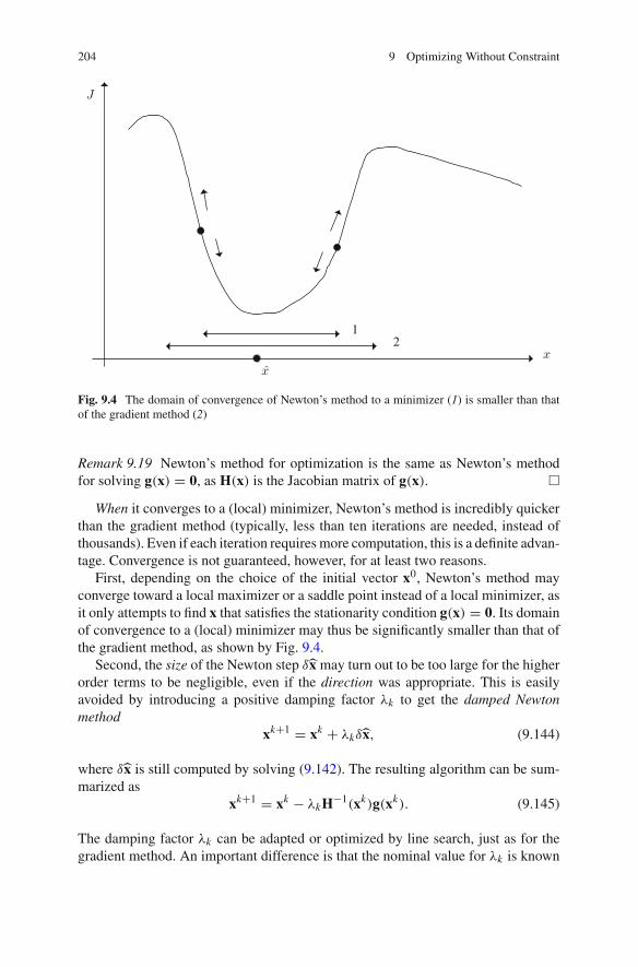
204 9 Optimizing Without Constraint

21

J

x

x

Fig. 9.4 The domain of convergence of Newton’s method to a minimizer (1) is smaller than thatof the gradient method (2)

Remark 9.19 Newton’s method for optimization is the same as Newton’s methodfor solving g(x) = 0, as H(x) is the Jacobian matrix of g(x). �

When it converges to a (local) minimizer, Newton’s method is incredibly quickerthan the gradient method (typically, less than ten iterations are needed, instead ofthousands). Even if each iteration requires more computation, this is a definite advan-tage. Convergence is not guaranteed, however, for at least two reasons.

First, depending on the choice of the initial vector x0, Newton’s method mayconverge toward a local maximizer or a saddle point instead of a local minimizer, asit only attempts to find x that satisfies the stationarity condition g(x) = 0. Its domainof convergence to a (local) minimizer may thus be significantly smaller than that ofthe gradient method, as shown by Fig. 9.4.

Second, the size of the Newton step ∂x may turn out to be too large for the higherorder terms to be negligible, even if the direction was appropriate. This is easilyavoided by introducing a positive damping factor βk to get the damped Newtonmethod

xk+1 = xk + βk ∂x, (9.144)

where ∂x is still computed by solving (9.142). The resulting algorithm can be sum-marized as

xk+1 = xk − βkH−1(xk)g(xk). (9.145)

The damping factor βk can be adapted or optimized by line search, just as for thegradient method. An important difference is that the nominal value for βk is known

9.3 Iterative Methods 205

here to be one, whereas there is no such nominal value in the case of the gradientmethod.

Newton’s method is particularly well suited to the final part of local search, whenthe gradient method has become too slow to be useful. Combining an initial behaviorsimilar to that of the gradient method and a final behavior similar to that of Newton’smethod thus makes sense. Before describing attempts at doing so, we consider animportant special case where Newton’s method can be usefully simplified.

9.3.4.3 Gauss-Newton Method

The Gauss-Newton method applies when the cost function can be expressed as a sumof N � dim x scalar terms that are quadratic in some error

J (x) =N⎡

l=1

wle2l (x), (9.146)

where the wl ’s are known positive weights. The error el (also called residual) may,for instance, be the difference between some measurement yl and the correspondingmodel output ym(l, x). The gradient of the cost function is then

g(x) = ∂ J

∂x(x) = 2

N⎡

l=1

wlel(x)∂el

∂x(x), (9.147)

where ∂el∂x (x) is the first-order sensitivity of the error with respect to x. The Hessian

of the cost can then be computed as

H(x) = ∂g∂xT (x) = 2

N⎡

l=1

wl

[∂el

∂x(x)

] [∂el

∂x(x)

]T

+ 2N⎡

l=1

wlel(x)∂2el

∂x∂xT (x),

(9.148)

where ∂2el∂x∂xT (x) is the second-order sensitivity of the error with respect to x. The

damped Gauss-Newton method is obtained by replacing H(x) in the damped Newtonmethod by the approximation

Ha(x) = 2N⎡

l=1

wl

[∂el

∂x(x)

] [∂el

∂x(x)

]T

. (9.149)

206 9 Optimizing Without Constraint

The damped Gauss-Newton step is thus

xk+1 = xk + βkdk, (9.150)

where dk is the solution of the linear system

Ha(xk)dk = −g(xk). (9.151)

Replacing H(xk) by Ha(xk) has two advantages. The first one, obvious, is that (atleast when dim x is small) the computation of the approximate Hessian Ha(x) requiresbarely more computation than that of the gradient g(x), as the difficult evaluation ofsecond-order sensitivities is avoided. The second one, more unexpected, is that thedamped Gauss-Newton method has the same domain of convergence to a given localminimizer as the gradient method, contrary to Newton’s method. This is due to thefact that Ha(x) → 0 (except in pathological cases), so H−1

a (x) → 0. As a result, theangle between the search direction −g(xk) of the gradient method and the searchdirection −H−1

a (xk)g(xk) of the Gauss-Newton method is less than π2 in absolute

value.When the magnitude of the residuals el(x) is small, the Gauss-Newton method

is much more efficient than the gradient method, at a limited additional computingcost per iteration. Performance tends to deteriorate, however, when this magnitudeincreases, because the neglected part of the Hessian gets too significant to be ignored[11]. This is especially true if el(x) is highly nonlinear in x, as the second-ordersensitivity of the error is then large. In such a situation, one may prefer a quasi-Newton method, see Sect. 9.3.4.5.

Remark 9.20 Sensitivity functions may be evaluated via forward automatic differ-entiation, see Sect. 6.6.4. �

Remark 9.21 When el = yl − ym(l, x), the first-order sensitivity of the error satisfies

∂

∂xel(x) = − ∂

∂xym(l, x). (9.152)

If ym(l, x) is obtained by solving ordinary or partial differential equations, then thefirst-order sensitivity of the model output ym with respect to xi can be computedby taking the first-order partial derivative of the model equations (including theirboundary conditions) with respect to xi and solving the resulting system of differen-tial equations. See Example 9.7. In general, computing the entire vector of first-ordersensitivities in addition to the model output thus requires solving (dim x+1) systemsof differential equations. For models described by ordinary differential equations,when the outputs of the model are linear with respect to its inputs and the initialconditions are zero, this number can be very significantly reduced by application ofthe superposition principle [10]. �

9.3 Iterative Methods 207

Example 9.7 Consider the differential model

q1 = −(x1 + x3)q1 + x2q2,

q2 = x1q1 − x2q2,

ym(t, x) = q2(t, x). (9.153)

with the initial conditionsq1(0) = 1, q2(0) = 0. (9.154)

Assume that the vector x of its parameters is to be estimated by minimizing

J (x) =N⎡

i=1

[y(ti ) − ym(ti , x)]2, (9.155)

where the numerical values of ti and y(ti ), (i = 1, . . . , N ) are known as the resultof experimentation on the system being modeled. The gradient and approximateHessian of the cost function (9.155) can be computed from the first-order sensitivityof ym with respect to the parameters. If s j,k is the first-order sensitivity of q j withrespect to xk ,

s j,k(ti , x) = ∂q j

∂xk(ti , x), (9.156)

then the gradient of the cost function is given by

g(x) =⎢

⎤−2

∑Ni=1[y(ti ) − q2(ti , x)]s2,1(ti , x)

−2∑N

i=1[y(ti ) − q2(ti , x)]s2,2(ti , x)

−2∑N

i=1[y(ti ) − q2(ti , x)]s2,3(ti , x)

⎥

⎞ ,

and the approximate Hessian by

Ha(x) = 2N⎡

i=1

⎢

⎣⎣⎣⎤

s22,1(ti , x) s2,1(ti , x)s2,2(ti , x) s2,1(ti , x)s2,3(ti , x)

s2,2(ti , x)s2,1(ti , x) s22,2(ti , x) s2,2(ti , x)s2,3(ti , x)

s2,3(ti , x)s2,1(ti , x) s2,3(ti , x)s2,2(ti , x) s22,3(ti , x)

⎥

⎦⎦⎦⎞ .

Differentiate (9.153) with respect to x1, x2 and x3 successively, to get

208 9 Optimizing Without Constraint

s1,1 = −(x1 + x3)s1,1 + x2s2,1 − q1,

s2,1 = x1s1,1 − x2s2,1 + q1,

s1,2 = −(x1 + x3)s1,2 + x2s2,2 + q2,

s2,2 = x1s1,2 − x2s2,2 − q2,

s1,3 = −(x1 + x3)s1,3 + x2s2,3 − q1,

s2,3 = x1s1,3 − x2s2,3. (9.157)

Since q(0) does not depend on x, the initial condition of each of the first-ordersensitivities is equal to zero

s1,1(0) = s2,1(0) = s1,2(0) = s2,2(0) = s1,3(0) = s2,3(0) = 0. (9.158)

The numerical solution of the system of eight first-order ordinary differential equa-tions (9.153, 9.157) for the initial conditions (9.154, 9.158) can be obtained bymethods described in Chap. 12. One may solve instead three systems of four first-order ordinary differential equations, each of them computing x1, x2 and the twosensitivity functions for one of the parameters. �

Remark 9.22 Define the error vector as

e(x) = [e1(x), e2(x), . . . , eN (x)]T, (9.159)

and assume that the wl ’s have been set to one by the method described in Sect. 9.2.1.Equation (9.151) can then be rewritten as

JT(xk)J(xk)dk = −JT(xk)e(xk), (9.160)

where J(x) is the Jacobian matrix of the error vector

J(x) = ∂e∂xT (x). (9.161)

Equation (9.160) is the normal equation for the linear least squares problem

dk = arg mind

‖J(xk)dk + e(xk)‖22, (9.162)

and a better solution for dk may be obtained by using one of the methods recom-mended in Sect. 9.2, for instance via a QR factorization of J(xk). An SVD of J(xk) ismore complicated but makes it trivial to monitor the conditioning of the local prob-lem to be solved. When the situation becomes desperate, it also allows regularizationto be carried out. �

9.3 Iterative Methods 209

9.3.4.4 Levenberg-Marquardt Method

Levenberg’s method [17] is a first attempt at combining the better properties of thegradient and Gauss-Newton methods in the context of minimizing a sum of squares.The displacement ∂x at iteration k is taken as the solution of the system of linearequations [

Ha(xk) + μkI]∂x = −g(xk), (9.163)

where the value given to the real scalar μk > 0 can be chosen by one-dimensionalminimization of J (xk + ∂x), seen as a function of μk .

When μk tends to zero, this method behaves as a (non-damped) Gauss-Newtonmethod, whereas when μk tends to infinity, it behaves as a gradient method with astep-size tending to zero.

To improve conditioning, Marquardt suggested in [18] to apply the same idea toa scaled version of (9.163):

[Hs

a + μkI]δs = −gs, (9.164)

with

hsi, j = hi, j√

hi,i√

h j, j, gs

i = gi√hi,i

and ∂si = ∂ xi√

hi,i, (9.165)

where hi, j is the entry of Ha(xk) in position (i, j), gi is the i th entry of g(xk) and∂ xi is the i th entry of ∂x. Since hi,i > 0, such a scaling is always possible. The i throw of (9.164) can then be written as

n⎡

j=1

(hs

i, j + μk∂i, j

)∂s

j = −gsi , (9.166)

where ∂i, j = 1 if i = j and ∂i, j = 0 otherwise. In terms of the original variables,(9.166) translates into

n⎡

j=1

(hi, j + μk∂i, j hi,i

)∂ x j = −gi . (9.167)

In other words, [Ha(xk) + μk · diag Ha(xk)

]∂x = −g(xk), (9.168)

where diag Ha is a diagonal matrix with the same diagonal entries as Ha. This is theLevenberg-Marquardt method, routinely used in software for nonlinear parameterestimation.

One disadvantage of this method is that a new system of linear equations has tobe solved whenever the value of μk is changed, which makes the optimization of μk

210 9 Optimizing Without Constraint

significantly more costly than with usual line searches. This is why some adaptivestrategy for tuning μk based on past behavior is usually employed. See [18] for moredetails.

The Levenberg-Marquardt method is one of those implemented in lsqnonlin,which is part of the MATLAB Optimization Toolbox.

9.3.4.5 Quasi-Newton Methods

Quasi-Newton methods [19] approximate the cost function J (x) after the kth iterationby a quadratic function of the decision vector x

Jq(x) = J (xk) + gTq (xk)(x − xk) + 1

2(x − xk)THq(x − xk), (9.169)

where

gq(xk) = ∂ Jq

∂x(xk) (9.170)

and

Hq = ∂2 Jq

∂x∂xT . (9.171)

Since the approximation is quadratic, its Hessian Hq does not depend on x, whichallows H−1

q to be estimated from the behavior of the algorithm along a series ofiterations.

Remark 9.23 Of course, J (x) is not exactly quadratic in x (otherwise, using the lin-ear least squares method of Sect. 9.2 would be a much better idea), but a quadraticapproximation usually becomes satisfactory when xk gets close enough to a mini-mizer. �

The updating of the estimate of x is directly inspired from the damped Newtonmethod (9.145), with H−1 replaced by the estimate Mk of H−1

q at iteration k:

xk+1 = xk − βkMkg(xk), (9.172)

where βk is again obtained by line search.Differentiate Jq(x) as given by (9.169) once with respect to x and evaluate the

result at xk+1 to get

gq(xk+1) = gq(xk) + Hq(xk+1 − xk), (9.173)

soHqκx = κgq, (9.174)

9.3 Iterative Methods 211

whereκgq = gq(xk+1) − gq(xk) (9.175)

andκx = xk+1 − xk . (9.176)

Equation (9.174) suggests the quasi-Newton equation

Hk+1κx = κg, (9.177)

with Hk+1 the approximation of the Hessian at iteration k + 1 and κg the variationof the gradient of the actual cost function between iterations k and k + 1. Thiscorresponds to (7.52), where the role of the function f(·) is taken by the gradientfunction g(·).

With Mk+1 = H−1k+1, (9.177) can be rewritten as

Mk+1κg = κx, (9.178)

which is used to update Mk as

Mk+1 = Mk + Ck . (9.179)

The correction term Ck must therefore satisfy

Ckκg = κx − Mkκg. (9.180)

Since H−1 is symmetric, its initial estimate M0 and the Ck’s are taken symmetric.This is an important difference with Broyden’s method of Sect. 7.4.3, as the Jacobianmatrix of a generic vector function is not symmetric.

Quasi-Newton methods differ by their expressions for Ck . The only possiblesymmetric rank-one correction is that of [20]:

Ck = (κx − Mkκg)(κx − Mkκg)T

(κx − Mkκg)Tκg, (9.181)

where it is assumed that (κx − Mkκg)Tκg ⊂= 0. It is trivial to check that it satisfies(9.180), but the matrices Mk generated by this scheme are not always positive definite.

Most quasi-Newton methods belong to a family defined in [20] and would givethe same results if computation were carried out exactly [21]. They differ, however,in their robustness to errors in the evaluation of gradients. The most popular of themis BFGS (an acronym for Broyden, Fletcher, Golfarb and Shanno, who published itindependently). BFGS uses the correction

Ck = C1 + C2, (9.182)

212 9 Optimizing Without Constraint

where

C1 =(

1 + κgTMkκgκxTκg

)κxκxT

κxTκg(9.183)

and

C2 = −κxκgTMk + MkκgκxT

κxTκg. (9.184)

It is easy to check that this update satisfies (9.180) and may also be written as

Mk+1 =(

I − κxκgT

κxTκg

)Mk

(I − κgκxT

κxTκg

)+ κxκxT

κxTκg. (9.185)

It is also easy to check that

κgTMk+1κg = κgTκx, (9.186)

so the line search for βk must ensure that

κgTκx > 0 (9.187)

for Mk+1 to be positive definite. This is the case when strong Wolf conditions areenforced during the computation of βk [22]. Other options include

• freezing M whenever κgTκx � 0 (by setting Mk+1 = Mk),• periodic restart, which forces Mk to the identity matrix every dim x iterations.

(If the actual cost function were quadratic in x and computation were carried outexactly, convergence would take place in at most dim x iterations.)

The initial value for the approximation of H−1 is taken as

M0 = I, (9.188)

so the method starts as a gradient method.Compared to Newton’s method, the resulting quasi-Newton methods have several

advantages:

• there is no need to compute the Hessian H of the actual cost function,• there is no need to solve a system of linear equations at each iteration, as an

approximation of H−1 is computed,• the domain of convergence to a minimizer is the same as for the gradient method

(provided that measures are taken to ensure that Mk → 0,√k � 0),• the estimate of the inverse of the Hessian can be used to study the local condition

number of the problem and to assess the precision with which the minimizer xhas been evaluated. This is important when estimating physical parameters fromexperimental data [10].

9.3 Iterative Methods 213

One should be aware, however, of the following drawbacks:

• quasi-Newton methods are rather sensitive to errors in the computation of thegradient, as they use differences of gradient values to update the estimate of H−1;they are more sensitive to such errors than the Gauss-Newton method, for instance;

• updating the (dim x × dim x) matrix Mk at each iteration may not be realistic ifdim x is very large as, e.g., in image processing.

The last of these drawbacks is one of the main reasons for considering insteadconjugate-gradient methods.

Quasi-Newton methods are widely used, and readily available in scientific routinelibraries. BFGS is one of those implemented in fminunc, which is part of theMATLAB Optimization Toolbox.

9.3.4.6 Conjugate-Gradient Methods

As the quasi-Newton methods, the conjugate-gradient methods [23, 24], approximatethe cost function by a quadratic function of the decision vector given by (9.169).Contrary to the quasi-Newton methods, however, they do not attempt to estimate Hqor its inverse, which makes them particularly suitable when dim x is very large.

The estimate of the minimizer is updated by line search along a direction dk ,according to

xk+1 = xk + βkdk . (9.189)

If dk were computed by Newton’s method, then it would satisfy,

dk = −H−1(xk)g(xk), (9.190)

and the optimization of βk should imply that

gT(xk+1)dk = 0. (9.191)

Since H(xk) is symmetric, (9.190) implies that

gT(xk+1) = −(dk+1)TH(xk+1), (9.192)

so (9.191) translates into(dk+1)TH(xk+1)dk = 0. (9.193)

Successive search directions of the optimally damped Newton method are thus con-jugate with respect to the Hessian. Conjugate-gradient methods will aim at achievingthe same property with respect to an approximation Hq of this Hessian. As the searchdirections under consideration are not gradients, talking of “conjugate-gradient” ismisleading, but imposed by tradition.

A famous member of the conjugate-gradient family is the Polack-Ribière method[16, 25], which takes

214 9 Optimizing Without Constraint

dk+1 = −g(xk+1) + ρPRk dk, (9.194)

where

ρPRk = [g(xk+1) − g(xk)]Tg(xk+1)

gT(xk)g(xk). (9.195)

If the cost function were actually given by (9.169), then this strategy would ensurethat dk+1 and dk are conjugate with respect to Hq, although Hq is neither knownnor estimated, a considerable advantage for large-scale problems. The method isinitialized by taking

d0 = −g(x0), (9.196)

so its starts like a gradient method. Just as with quasi-Newton methods, a periodicrestart strategy may be employed, with dk taken equal to −g(xk) every dim x itera-tions.

Satisfaction of strong Wolfe conditions during line search does not guarantee,however that dk+1 as computed with the Polack-Ribière method is always a descentcondition [11]. To fix this, it suffices to replace ρPR

k in (9.194) by

ρPR+k = max{ρPR, 0}. (9.197)

The main drawback of conjugate gradients compared to quasi-Newton is that theinverse of the Hessian is not estimated. One may thus prefer quasi-Newton if dim xis small enough and one is interested in evaluating the local condition number of theoptimization problem or in characterizing the uncertainty on x.

Example 9.8 A killer applicationAs already mentioned in Sect. 3.7.2.2, conjugate gradients are used for solving

large systems of linear equationsAx = b, (9.198)

with A symmetric and positive definite. Such systems may, for instance, correspondto the normal equations of least squares. Solving (9.198) is equivalent to minimizingthe square of a suitably weighted quadratic norm

J (x) = ||Ax − b||2A−1 = (Ax − b)TA−1(Ax − b) (9.199)

= bTA−1b − 2bTx + xTAx, (9.200)

which is in turn equivalent to minimizing

J (x) = xTAx − 2bTx. (9.201)

The cost function (9.201) is exactly quadratic, so its Hessian does not depend on x,and using the conjugate-gradient method entails no approximation. The gradient ofthe cost function, needed by the method, is easy to compute as

9.3 Iterative Methods 215

g(x) = 2(Ax − b). (9.202)

A good approximation of the solution is often obtained with this approach in muchless than the dim x iterations theoretically needed. �

9.3.4.7 Convergence Speeds and Complexity Issues

When xk gets close enough to a minimizer x (which may be local or global), itbecomes possible to study the (asymptotic) convergence speed of the main iterativeoptimization methods considered so far [11, 19, 26]. We assume here that J (·) istwice continuously differentiable and that H(x) is symmetric positive definite, so allof its eigenvalues are real and strictly positive.

A gradient method with optimization of the step-size has a linear convergencespeed, as

lim supk→∞

‖xk+1 − x‖‖xk − x‖ = σ, with σ < 1. (9.203)

Its convergence rate σ satisfies

σ �(

βmax − βmin

βmax + βmin

)2

, (9.204)

with βmax and βmin the largest and smallest eigenvalues of H(x), which are also itslargest and smallest singular values. The most favorable situation is when all theeigenvalues of H(x) are equal, so βmax = βmin, cond H(x) = 1 and σ = 0. Whenβmax � βmin, cond H(x) � 1 and σ is close to one so convergence becomes veryslow.

Newton’s method has a quadratic convergence speed, provided that H(·) satisfiesa Lipschitz condition at x, i.e., there exists κ such that

√x, ‖H(x) − H(x)‖ � κ‖x − x‖. (9.205)

This is much better than a linear convergence speed. As long as the effect of roundingcan be neglected, the number of correct decimal digits in xk is approximately doubledat each iteration.

The convergence speed of the Gauss-Newton or Levenberg-Marquardt methodlies somewhere between linear and quadratic, depending on the quality of the approx-imation of the Hessian, which itself depends on the magnitude of the residuals. Whenthis magnitude is small enough convergence is quadratic, but for large enough resid-uals it becomes linear.

Quasi-Newton methods have a superlinear convergence speed, so

216 9 Optimizing Without Constraint

lim supk→∞

‖xk+1 − x‖‖xk − x‖ = 0. (9.206)

Conjugate-gradient methods also have a superlinear convergence speed, but on dim xiterations. They thus require approximately (dim x) times as many iterations as quasi-Newton methods to achieve the same asymptotic behavior. With periodic restart everyn = dim x iteration, conjugate gradient methods can even achieve n-step quadraticconvergence, that is

lim supk→∞

‖xk+n − x‖‖xk − x‖2 = σ < ∞. (9.207)

(In practice, restart may never take place if n is large enough.)

Remark 9.24 Of course, rounding limits the accuracy with which x can be evaluatedwith any of these methods. �

Remark 9.25 These results say nothing about non-asymptotic behavior. A gradientmethod may still be much more efficient in the initial phase of search than Newton’smethod. �

Complexity must also be taken into consideration in the choice of a method. Ifthe effort needed for evaluating the cost function and its gradient (plus its Hessianfor the Newton method) can be neglected, a Newton iteration requires O(n3) flops,to be compared with O(n2) flops for a quasi-Newton iteration and O(n) flops for aconjugate-gradient iteration. On a large-scale problem, a conjugate-gradient iterationthus requires much less computation and memory than a quasi-Newton iteration,which itself requires much less computation than a Newton iteration.

9.3.4.8 Where to Start From and When to Stop?

Most of what has been said in Sects. 7.5 and 7.6 remains valid. When the cost functionis convex and differentiable, there is a single local minimizer, which is also global,and the methods described so far should converge to this minimizer from any initialpoint x0. Otherwise, it is still advisable to use multistart, unless one can afford onlyone local minimization (having a good enough initial point then becomes critical).In principle, local search should stop when all the components of the gradient of thecost function are zero, so the stopping criteria are similar to those used when solvingsystems of nonlinear equations.

9.3.5 A Method That Can Deal with Nondifferentiable Costs

None of the methods based on a Taylor expansion works if the cost function J (·) isnot differentiable. Even when J (·) is differentiable almost everywhere, e.g., when it

9.3 Iterative Methods 217

is a sum of absolute values of differentiable errors as in (8.15), these methods willgenerally rush to points where they are no longer valid.

A number of sophisticated approaches have been designed for minimizing nondif-ferentiable cost functions, based, for instance, on the notion of sub-gradient [27–29],but they are out of the scope of this book. This section presents only one methodthat can be used when the cost function is not differentiable, the celebrated Nelderand Mead simplex method [30], not to be confused with Dantzig’s simplex methodfor linear programming, to be considered in Sect. 10.6. Alternative approaches arein Sect. 9.4.2.1 and Chap. 11.

Remark 9.26 The Nelder and Mead method does not require the cost function tobe differentiable, but can of course also be used on differentiable functions. It turnsout to be a remarkably useful (and enormously popular) general-purpose workhorse,although surprisingly little is known about its theoretical properties [31, 32]. It isimplemented in MATLAB as fminsearch. �

A simplex in Rn is a convex polytope with (n + 1) vertices (a triangle when

n = 2, a tetrahedron when n = 3, and so on). The basic idea of the Nelder and Meadmethod is to evaluate the cost function at each vertex of a simplex in search space,and to deduce from the resulting values of the cost how to transform this simplexfor the next iteration so as to crawl toward a (local) minimizer. A two-dimensionalsearch space will be used here for illustration, but the method may be used in higherdimensional spaces.

Three vertices of the current simplex will be singled out by specific names:

• b is the best vertex (in terms of cost),• w is the worst vertex (we want to move away from it; it will always be rejected in

the next simplex, and its nickname is wastebasket vertex),• s is the next-to-the-worst vertex.

Thus,J (b) � J (s) � J (w). (9.208)

A few more points play special roles:

• c is such that its coordinates are the arithmetic means of the coordinates of the nbest vertices, i.e., all the vertices except w,

• tref, texp, tin and tout are trial points.

An iteration of the algorithm starts by a reflection (Fig. 9.5), during which thetrial point is chosen as the symmetric of the worst current vertex with respect to thecenter of gravity c of the face opposed to it

tref = c + (c − w) = 2c − w. (9.209)

If J (b) � J (tref) � J (s), then w is replaced by tref. If the reflection has been moresuccessful and J (tref) < J (b), then the algorithm tries to go further in the samedirection. This is expansion (Fig. 9.6), where the trial point becomes

218 9 Optimizing Without Constraint

Fig. 9.5 Reflection (potentialnew simplex is in grey)

w

b

s

c

tref

Fig. 9.6 Expansion (potentialnew simplex is in grey)

texp

w s

c

b

texp = c + 2(c − w). (9.210)

If the expansion is a success, i.e., if J (texp) < J (tref), then w is replaced by texp,else it is still replaced by tref.

Remark 9.27 Some the vertices kept from one iteration to the next must be renamed.For instance, after a successful expansion, the trial point texp becomes the best ver-tex b. �

When reflection is more of a failure, i.e., when J (tref) > J (s), two types ofcontractions are considered (Fig. 9.7). If J (tref) < J (w), then a contraction on thereflexion side (or outside contraction) is attempted, with the trial point

tout = c + 1

2(c − w) = 1

2(c + tref), (9.211)

whereas if J (tref) � J (w) a contraction on the worst side (or inside contraction) isattempted, with the trial point

9.3 Iterative Methods 219

w

tin

b

s

c

tout

Fig. 9.7 Contractions (potential new simplices are in grey)b

sw

Fig. 9.8 Shrinkage (new simplex is in grey)

tin = c − 1

2(c − w) = 1

2(c + w). (9.212)

Let t be the best out of tref and tin (or tref and tout). If J (t) < J (w), then the worstvertex w is replaced by t.

Else, a shrinkage is performed (Fig. 9.8), during which each other vertex is movedin the direction of the best vertex by halving its distance to b, before starting a newiteration of the algorithm, by a reflection.

Iterations are stopped when the volume of the current simplex dwindles belowsome threshold.

220 9 Optimizing Without Constraint

9.4 Additional Topics

This section briefly mentions extensions of unconstrained optimization methods thatare aimed at

• taking into account the effect of perturbations on the value of the performanceindex,

• avoiding being trapped at local minimizers that are not global,• decreasing the number of evaluations of the cost function to comply with budget

limitations,• dealing with situations where conflicting objectives have to be taken into account.

9.4.1 Robust Optimization

Performance often depends not only on some decision vector x but also on the effectof perturbations. It is assumed here that these perturbations can be characterized by avector p on which some prior information is available, and that a performance indexJ (x, p) can be computed. The prior information on p may take either of two forms:

• a known probability distribution π(p) for p (for instance, one may assume that pis a Gaussian random vector, and that its mean is 0 and its covariance matrix σ2 I,with σ2 known),

• a known feasible set P to which p belongs (defined, for instance, by lower andupper bounds for each of the components of p).

In both cases, one wants to choose x optimally while taking into account the effectof p. This is robust optimization, to which considerable attention is being devoted[33, 34]. The next two sections present two methods that can be used in this context,one for each type of prior information on p.

9.4.1.1 Average-Case Optimization

When a probability distribution π(p) for the perturbation vector p is available, onemay average p out by looking for

x = arg minx

Ep{J (x, p)}, (9.213)

where Ep{·} is the mathematical-expectation operator with respect to p. The gradientmethod for computing iteratively an approximation of x would then be

xk+1 = xk − βkg(xk), (9.214)

with

9.4 Additional Topics 221

g(x) = ∂

∂x[Ep{J (x, p)}]. (9.215)

Each iteration would thus require the evaluation of the gradient of a mathematicalexpectation, which might be extremely costly as it might involve numerical evalua-tions of multidimensional integrals.

The stochastic gradient method, a particularly simple example of a stochasticapproximation technique, computes instead

xk+1 = xk − βkg∈(xk), (9.216)

with

g∈(x) = ∂

∂x[J (x, pk)], (9.217)

where pk is picked at random according to π(p) and βk should satisfy the threefollowing conditions:

• βk > 0 (for the steps to be in the right direction),• ∑∞

k=0 βk = ∞ (for all possible values of x to be reachable),• ∑∞

k=0 β2k < ∞ (for xk to converge toward a constant vector when k tends to

infinity).

One may use, for instance

βk = β0

k + 1,

with β0 > 0 to be chosen by the user. More sophisticated options are available; see,e.g., [10]. The stochastic gradient method makes it possible to minimize a mathe-matical expectation without ever evaluating it or its gradient. As this is still a localmethod, convergence to a global minimizer of Ep{J (x, p)} is not guaranteed andmultistart remains advisable.

An interesting special case is when p can only take the values pi , i = 1, . . . , N ,with N finite (but possibly very large), and each pi has the same probability 1/N .Average-case optimization then boils down to computing

x = arg minx

J ∈(x), (9.218)

with

J ∈(x) = 1

N

N⎡

i=1

Ji (x), (9.219)

where

Ji (x) = J (x, pi ). (9.220)

222 9 Optimizing Without Constraint

Provided that each function Ji (·) is smooth and J ∈(·) is strongly convex (as is oftenthe case in machine learning), the stochastic average gradient algorithm presentedin [35] can dramatically outperform a conventional stochastic gradient algorithm interms of convergence speed.

9.4.1.2 Worst-Case Optimization

When a feasible set P for the perturbation vector p is available, one may look for thedesign vector x that is best under the worst circumstances, i.e.,

x = arg minx

[maxp∇P

J (x, p)]. (9.221)

This is minimax optimization [36], commonly encountered in Game Theory wherex and p characterize the decisions taken by two players. The fact that P is here acontinuous set makes the problem particularly difficult to solve. The naive approcheknown as best replay, which alternates minimization of J with respect to x for thecurrent value of p and maximization of J with respect to p for the current value of x,may cycle hopelessly. Brute force, on the other hand, where two nested optimizationsare carried out, is usually too complicated to be useful, unless P is approximated bya finite set P with sufficiently few elements to allow maximization with respect top by exhaustive search. The relaxation method [37] builds P iteratively, as follows:

1. Take P = {p1}, where p1 is picked at random in P, and k = 1.2. Find xk = arg minx[maxp∇P J (x, p)].3. Find pk+1 = arg maxp∇P J (xk, p).4. If J (xk, pk+1) � maxp∇P J (xk, p) + ∂, where ∂ > 0 is a user-chosen tolerance

parameter, then accept xk as an approximation of x. Else, take P := P∪{pk+1},increment k by one and go to Step 2.

This method leaves open the choice of the optimization routines to be employedat Steps 2 and 3. Under reasonable technical conditions, it stops after a finite numberof iterations.

9.4.2 Global Optimization

Global optimization looks for the global optimum of the cost function, and the asso-ciate value(s) of the global optimizer(s). It thus bypasses the initialization problemsraised by local methods. Two complementary approaches are available, which differby the type of search carried out. Random search is easy to implement and can beused on large classes of problems but does not guarantee success, whereas deter-ministic search [38] is more complicated and less generally applicable but makes itpossible to make guaranteed statements about the global optimizer(s) and optimum.

9.4 Additional Topics 223

The next two sections briefly describe examples of the two strategies. In both cases,search is assumed to take place in a possibly very large domain X taking the form ofan axis-aligned hyper-rectangle, or box. As no global optimizer is expected to belongto the boundary of X, this is still unconstrained optimization.

Remark 9.28 When a vector x of model parameters must be estimated from experi-mental data by minimizing the l p-norm of an error vector (p = 1, 2,∞), appropriateexperimental conditions may eliminate all suboptimal local minimizers, thus allow-ing local methods to be used to get a global minimizer [39]. �

9.4.2.1 Random Search

Multistart is a particularly simple example of random search. A number of moresophisticated strategies have been inspired by biology (with genetic algorithms [40,41] and differential evolution [42]), behavioral sciences (with ant-colony algorithms[43] and particle-swarm optimization [44]) and metallurgy (with simulated anneal-ing, see Sect. 11.2). Most random-search algorithms have internal parameters thatmust be tuned and have significant impact on their behavior, and one should not forgetthe time spent tuning these parameters when assessing performance on a given appli-cation. Adaptive Random Search (ARS) [45] has shown in [46] its ability to solvevarious test-cases and real-life problems while using the same tuning of its internalparameters. The description of ARS presented here corresponds to typical choices,to which there are perfectly valid alternatives. (One may, for instance, use uniformdistributions instead of Gaussian distributions to generate random displacements.)

Five versions of the following basic algorithm are made to compete:

1. Choose x0, set k = 0.2. Pick a trial point xk+ = xk + δk , with δk random.3. If J (xk+) < J (xk) then xk+1 = xk+, else xk+1 = xk .4. Increment k by one and go to Step 2.

In the j th version of this algorithm ( j = 1, . . . , 5), a Gaussian distributionN (0,λ( jσ)) is used to generate δk , with a diagonal covariance matrix

λ( jσ) = diag⎠

jσ2i , i = 1, . . . , dim x

}, (9.222)

and truncation is carried out to ensure that xk+ stays in X. The distributions differby the value given to j σ, j = 1, . . . , 5. One may take, for instance,

1σi = xmaxi − xmin

i , i = 1, . . . , dim x, (9.223)

to promote large displacements in X, and

j σ = j−1 σ /10, j = 2, . . . , 5. (9.224)

224 9 Optimizing Without Constraint

to favor finer and finer explorations.A variance-selection phase and a variance-exploitation phase are alternated. In the

variance-selection phase, the five competing basic algorithms are run from the sameinitial point (the best x available at the start of the phase). Each algorithm is given100/ i iterations, to give more trials to larger variances. The one with the best results(in terms of the final value of the cost) is selected for the next variance-exploitationphase, during which it is initialized at the best x available and used for 100 iterationsbefore resuming a variance-selection phase.

One may optionally switch to a local optimization routine whenever 5 σ is selected,as it corresponds to very small displacements. Search is stopped when the budgetfor the evaluation of the cost function is exhausted or when 5 σ has been selected agiven number of times consecutively.

This algorithm is extremely simple to implement, and does not require the costfunction to be differentiable. It is so flexible to use that it encourages creativity intailoring cost functions. It may escape parasitic local minimizers, but no guaranteecan be provided as to its ability to find a global minimizer in a finite number ofiterations.

9.4.2.2 Guaranteed Optimization

A key concept allowing the proof of statements about the global minimizers ofnonconvex cost functions is that of branch and bound. Branching partitions the initialfeasible set X into subsets, while bounding computes bounds on the values taken byquantities of interest over each of the resulting subsets. This makes it possible toprove that some subsets contain no global minimizer of the cost function over X andthus to eliminate them from subsequent search. Two examples of such proofs are asfollows:

• if a lower bound of the value of the cost function over Xi ⊂ X is larger than anupper bound of the minimum of the cost function over X j ⊂ X, then X

i containsno global minimizer,

• if at least one component of the gradient of the cost function is such that its upperbound over Xi ⊂ X is strictly negative (or its lower bound strictly positive), thenthe necessary condition for optimality (9.6) is nowhere satisfied on X

i , whichtherefore contains no (unconstrained) local or global minimizer.

Any subset of X that cannot be eliminated may contain a global minimizer of thecost function over X. Branching may then be used to split it into smaller subsets onwhich bounding is carried out. It is sometimes possible to locate all global minimizersvery accurately with this type of approach.

Interval analysis (see Sect. 14.5.2.3 and [47–50]) is a good provider of boundson the values taken by the cost function and its derivatives over subsets of X, andtypical interval-based algorithms for global optimization can be found in [51–53].

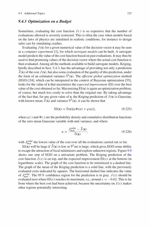
9.4 Additional Topics 225

9.4.3 Optimization on a Budget

Sometimes, evaluating the cost function J (·) is so expensive that the number ofevaluations allowed is severely restricted. This is often the case when models basedon the laws of physics are simulated in realistic conditions, for instance to designsafer cars by simulating crashes.

Evaluating J (x) for a given numerical value of the decision vector x may be seenas a computer experiment [1], for which surrogate models can be built. A surrogatemodel predicts the value of the cost function based on past evaluations. It may thus beused to find promising values of the decision vector where the actual cost function isthen evaluated. Among all the methods available to build surrogate models, Kriging,briefly described in Sect. 5.4.3, has the advantage of providing not only a predictionJ (x) of the cost J (x), but also some evaluation of the quality of this prediction, underthe form of an estimated variance σ2(x). The efficient global optimization method(EGO) [54], which can be interpreted in the context of Bayesian optimization [55],looks for the value of x that maximizes the expected improvement (EI) over the bestvalue of the cost obtained so far. Maximizing EI(x) is again an optimization problem,of course, but much less costly to solve than the original one. By taking advantageof the fact that, for any given value of x, the Kriging prediction of J (x) is Gaussian,with known mean J (x) and variance σ2(x), it can be shown that

EI(x) = σ(x)[u (u) + ϕ(u)], (9.225)

where ϕ(·) and (·) are the probability density and cumulative distribution functionsof the zero-mean Gaussian variable with unit variance, and where

u = J sofarbest − J (x)

σ(x), (9.226)

with J sofarbest the lowest value of the cost over all the evaluations carried out so far.

EI(x) will be large if J (x) is low or σ2(x) is large, which gives EGO some abilityto escape the attraction of local minimizers and explore unknown regions. Figure 9.9shows one step of EGO on a univariate problem. The Kriging prediction of thecost function J (x) is on top, and the expected improvement EI(x) at the bottom (inlogarithmic scale). The graph of the cost function to be minimized is a dashed line.The graph of the mean of the Kriging prediction is a solid line, with the previouslyevaluated costs indicated by squares. The horizontal dashed line indicates the valueof J sofar

best . The 95 % confidence region for the prediction is in grey. J (x) should beevaluated next where EI(x) reaches its maximum, i.e., around x = −0.62. This is farfrom where the best cost had been achieved, because the uncertainty on J (x) makesother regions potentially interesting.

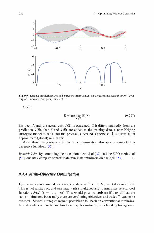
226 9 Optimizing Without Constraint

x

EI(x)

–6

–4

–2

–2

–1

–1

–1

–0.5

–0.5

0

0

0

0

0.5

0.5

1

1

1

2

Fig. 9.9 Kriging prediction (top) and expected improvement on a logarithmic scale (bottom) (cour-tesy of Emmanuel Vazquez, Supélec)

Once

x = arg maxx∇X

EI(x) (9.227)

has been found, the actual cost J (x) is evaluated. If it differs markedly from theprediction J (x), then x and J (x) are added to the training data, a new Krigingsurrogate model is built and the process is iterated. Otherwise, x is taken as anapproximate (global) minimizer.

As all those using response surfaces for optimization, this approach may fail ondeceptive functions [56].

Remark 9.29 By combining the relaxation method of [37] and the EGO method of[54], one may compute approximate minimax optimizers on a budget [57]. �

9.4.4 Multi-Objective Optimization

Up to now, it was assumed that a single scalar cost function J (·) had to be minimized.This is not always so, and one may wish simultaneously to minimize several costfunctions Ji (x) (i = 1, . . . , nJ). This would pose no problem if they all had thesame minimizers, but usually there are conflicting objectives and tradeoffs cannot beavoided. Several strategies make it possible to fall back on conventional minimiza-tion. A scalar composite cost function may, for instance, be defined by taking some

9.4 Additional Topics 227

linear combination of the individual cost functions

J (x) =nJ⎡

i=1

wi Ji (x), (9.228)

with positive weights wi to be chosen by the user. One may also give priority to oneof the cost functions and minimize it under constraints on the values allowed to theothers (see Chap. 10).

These two strategies restrict choice, however, and one may prefer to look for thePareto front, i.e., the set of all x ∇ X such that any local move that decreases agiven cost Ji increases at least one of the other costs. The Pareto front is thus a setof tradeoff solutions. Computing a Pareto front is of course much more complicatedthat minimizing a single cost function [58]. A single decision x has usually to betaken at a later stage anyway, which corresponds to minimizing (9.228) for a specificchoice of the weights wi . An examination of the shape of the Pareto front may helpthe user choose the most appropriate tradeoff.

9.5 MATLAB Examples

These examples deal with the estimation of the parameters of a model from experi-mental data. In both of them, these data have been generated by simulating the modelfor some known true value of the parameter vector, but this knowledge cannot beused in the estimation procedure, of course. No simulated measurement noise hasbeen added. Although rounding errors are unavoidable, the value of the norm of theerror between the data and best model output should thus be close to zero, and theoptimal parameters should be close to their true values.

9.5.1 Least Squares on a Multivariate Polynomial Model

The parameter vector p of the four-input one-output polynomial model

ym(x, p) = p1 + p2x1 + p3x2 + p4x3 + p5x4 + p6x1x2 + p7x1x3

+ p8x1x4 + p9x2x3 + p10x2x4 + p11x3x4 (9.229)

is to be estimated from the data (yi , xi ), i = 1, . . . , N . For any given value xi of theinput vector, the corresponding datum is computed as

yi = ym(xi , p�), (9.230)

where p� is the true value of the parameter vector, arbitrarily chosen as

228 9 Optimizing Without Constraint

p� = (10,−9, 8,−7, 6,−5, 4,−3, 2,−1, 0)T. (9.231)

The estimate p is computed as

p = arg minp∇R11

J (p), (9.232)

where

J (p) =N⎡

i=1

[yi − ym(xi , p)]2. (9.233)

Since ym(xi , p) is linear in p, linear least squares apply. The feasible domain X forthe input vector xi is defined as the Cartesian product of the feasible ranges for eachof the input factors. The j th input factor can take any value in [min(j), max(j)],with

min(1) = 0; max(1) = 0.05;min(2) = 50; max(2) = 100;min(3) = -1; max(3) = 7;min(4) = 0; max(4) = 1.e5;

The feasible ranges for the four input factors are thus quite different, which tends tomake the problem ill-conditioned.

Two designs for data collection are considered. In Design D1, each xi is inde-pendently picked at random in X, whereas Design D2 is a two-level full factorialdesign, in which the data are collected at all the possible combinations of the boundsof the ranges of the input factors. Design D2 thus has 24 = 16 different experimentalconditions xi . In what follows, the number N of pairs (yi , xi ) of data points in D1 istaken equal to 32, so D2 is repeated twice to get the same number of data points asin D1.

The output data are in Y for D1 and in Yfd for D2, while the corresponding valuesof the factors are in X for D1 and in Xfd, for D2. The following function is usedfor estimating the parameters P from the output data Y and corresponding regressionmatrix F

function[P,Cond] = LSforExample(F,Y,option)% F is (nExp,nPar), contains the regression matrix.% Y is (nExp,1), contains the measured outputs.% option specifies how the LS estimate is computed;% it is equal to 1 for NE, 2 for QR and 3 for SVD.% P is (nPar,1), contains the parameter estimate.% Cond is the condition number of the system solved% by the approach selected (for the spectral norm).[nExp,nPar] = size(F);

9.5 MATLAB Examples 229

if (option == 1)% Computing P by solving the normal equationsP = (F’*F)\F’*Y;% here, \ is by Gaussian eliminationCond = cond(F’*F);

end

if (option == 2)% Computing P by QR factorization[Q,R] = qr(F);QTY = Q’*Y;opts_UT.UT = true;P = linsolve(R,QTY,opts_UT);Cond = cond(R);

end

if (option == 3)% Computing P by SVD[U,S,V] = svd(F,’econ’);P = V*inv(S)*U’*Y;Cond = cond(S);

endend

9.5.1.1 Using Randomly Generated Experiments

Let us first process the data collected according to D1, with the script

% Filing the regression matrixF = zeros(nExp,nPar);for i=1:nExp,

F(i,1) = 1;F(i,2) = X(i,1);F(i,3) = X(i,2);F(i,4) = X(i,3);F(i,5) = X(i,4);F(i,6) = X(i,1)*X(i,2);F(i,7) = X(i,1)*X(i,3);F(i,8) = X(i,1)*X(i,4);F(i,9) = X(i,2)*X(i,3);F(i,10) = X(i,2)*X(i,4);F(i,11) = X(i,3)*X(i,4);

end% Condition number of initial problem

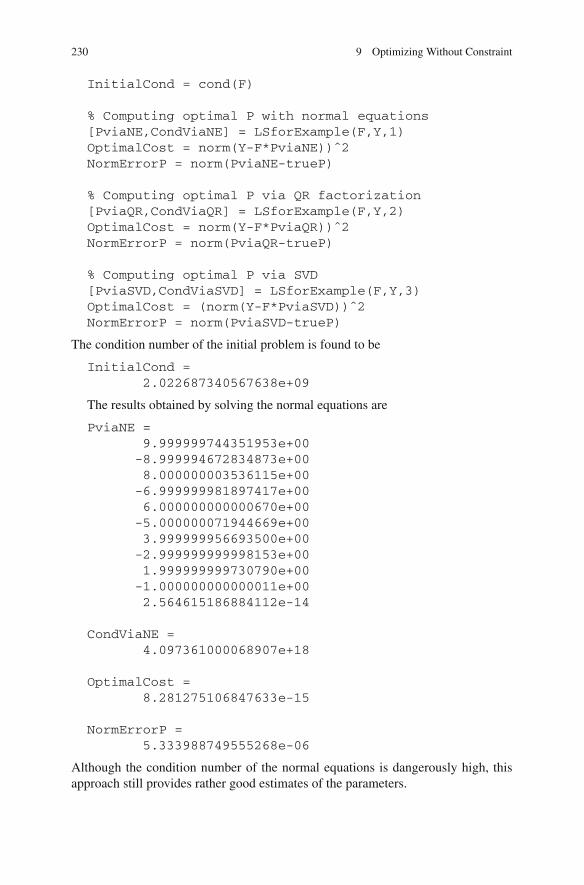
230 9 Optimizing Without Constraint

InitialCond = cond(F)

% Computing optimal P with normal equations[PviaNE,CondViaNE] = LSforExample(F,Y,1)OptimalCost = norm(Y-F*PviaNE))ˆ2NormErrorP = norm(PviaNE-trueP)

% Computing optimal P via QR factorization[PviaQR,CondViaQR] = LSforExample(F,Y,2)OptimalCost = norm(Y-F*PviaQR))ˆ2NormErrorP = norm(PviaQR-trueP)

% Computing optimal P via SVD[PviaSVD,CondViaSVD] = LSforExample(F,Y,3)OptimalCost = (norm(Y-F*PviaSVD))ˆ2NormErrorP = norm(PviaSVD-trueP)

The condition number of the initial problem is found to be

InitialCond =2.022687340567638e+09

The results obtained by solving the normal equations are

PviaNE =9.999999744351953e+00-8.999994672834873e+008.000000003536115e+00-6.999999981897417e+006.000000000000670e+00-5.000000071944669e+003.999999956693500e+00-2.999999999998153e+001.999999999730790e+00-1.000000000000011e+002.564615186884112e-14

CondViaNE =4.097361000068907e+18

OptimalCost =8.281275106847633e-15

NormErrorP =5.333988749555268e-06

Although the condition number of the normal equations is dangerously high, thisapproach still provides rather good estimates of the parameters.

9.5 MATLAB Examples 231

The results obtained via a QR factorization of the regression matrix are

PviaQR =9.999999994414727e+00-8.999999912908700e+008.000000000067203e+00-6.999999999297954e+006.000000000000007e+00-5.000000001454850e+003.999999998642462e+00-2.999999999999567e+001.999999999988517e+00-1.000000000000000e+003.038548268619260e-15

CondViaQR =2.022687340567638e+09

OptimalCost =4.155967155703225e-17

NormErrorP =8.729574294487699e-08

The condition number of the initial problem is recovered, and the parameter estimatesare more accurate than when solving the normal equations.

The results obtained via an SVD of the regression matrix are

PviaSVD =9.999999993015081e+00-9.000000089406967e+008.000000000036380e+00-7.000000000407454e+006.000000000000076e+00-5.000000000232831e+004.000000002793968e+00-2.999999999999460e+002.000000000003638e+00-1.000000000000000e+00-4.674038933671909e-14

CondViaSVD =2.022687340567731e+09

OptimalCost =5.498236550294591e-15

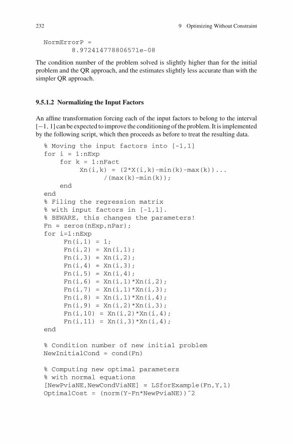
232 9 Optimizing Without Constraint

NormErrorP =8.972414778806571e-08

The condition number of the problem solved is slightly higher than for the initialproblem and the QR approach, and the estimates slightly less accurate than with thesimpler QR approach.

9.5.1.2 Normalizing the Input Factors

An affine transformation forcing each of the input factors to belong to the interval[−1, 1] can be expected to improve the conditioning of the problem. It is implementedby the following script, which then proceeds as before to treat the resulting data.

% Moving the input factors into [-1,1]for i = 1:nExp

for k = 1:nFactXn(i,k) = (2*X(i,k)-min(k)-max(k))...

/(max(k)-min(k));end

end% Filing the regression matrix% with input factors in [-1,1].% BEWARE, this changes the parameters!Fn = zeros(nExp,nPar);for i=1:nExp

Fn(i,1) = 1;Fn(i,2) = Xn(i,1);Fn(i,3) = Xn(i,2);Fn(i,4) = Xn(i,3);Fn(i,5) = Xn(i,4);Fn(i,6) = Xn(i,1)*Xn(i,2);Fn(i,7) = Xn(i,1)*Xn(i,3);Fn(i,8) = Xn(i,1)*Xn(i,4);Fn(i,9) = Xn(i,2)*Xn(i,3);Fn(i,10) = Xn(i,2)*Xn(i,4);Fn(i,11) = Xn(i,3)*Xn(i,4);

end

% Condition number of new initial problemNewInitialCond = cond(Fn)

% Computing new optimal parameters% with normal equations[NewPviaNE,NewCondViaNE] = LSforExample(Fn,Y,1)OptimalCost = (norm(Y-Fn*NewPviaNE))ˆ2

9.5 MATLAB Examples 233

% Computing new optimal parameters% via QR factorization[NewPviaQR,NewCondViaQR] = LSforExample(Fn,Y,2)OptimalCost = (norm(Y-Fn*NewPviaQR))ˆ2

% Computing new optimal parameters via SVD[NewPviaSVD,NewCondViaSVD] = LSforExample(Fn,Y,3)OptimalCost = (norm(Y-Fn*NewPviaSVD))ˆ2

The condition number of the transformed problem is found to be

NewInitialCond =5.633128746769874e+00

It is thus much better than for the initial problem.The results obtained by solving the normal equations are

NewPviaNE =-3.452720300000000e+06-3.759299999999603e+03-1.249653125000001e+065.723999999996740e+02-3.453750000000000e+06-3.124999999708962e+003.999999997322448e-01-3.750000000000291e+032.000000000006985e+02-1.250000000000002e+067.858034223318100e-10

NewCondViaNE =3.173213947768512e+01

OptimalCost =3.218047573208537e-17

The results obtained via a QR factorization of the regression matrix are

NewPviaQR =-3.452720300000001e+06-3.759299999999284e+03-1.249653125000001e+065.724000000002399e+02-3.453750000000001e+06-3.125000000827364e+003.999999993921934e-01-3.750000000000560e+03

234 9 Optimizing Without Constraint

2.000000000012406e+02-1.250000000000000e+062.126983788033481e-09

NewCondViaQR =5.633128746769874e+00

OptimalCost =7.951945308823372e-17

Although the condition number of the transformed initial problem is recovered, thesolution is actually slightly less accurate than when solving the normal equations.

The results obtained via an SVD of the regression matrix are

NewPviaSVD =-3.452720300000001e+06-3.759299999998882e+03-1.249653125000000e+065.724000000012747e+02-3.453749999999998e+06-3.125000001688022e+003.999999996158294e-01-3.750000000000931e+032.000000000023283e+02-1.250000000000001e+061.280568540096283e-09

NewCondViaSVD =5.633128746769864e+00

OptimalCost =1.847488972244773e-16

Once again, the solution obtained via SVD is slightly less accurate than the oneobtained via QR factorization. So the approach solving the normal equations is aclear winner on this version of the problem, as it is the less expensive and the mostaccurate.

9.5.1.3 Using a Two-Level Full Factorial Design

Let us finally process the data collected according to D2, defined as follows.

% Two-level full factorial design% for the special case nFact = 4FD = [-1, -1, -1, -1;

-1, -1, -1, +1;-1, -1, +1, -1;

9.5 MATLAB Examples 235

-1, -1, +1, +1;-1, +1, -1, -1;-1, +1, -1, +1;-1, +1, +1, -1;-1, +1, +1, +1;+1, -1, -1, -1;+1, -1, -1, +1;+1, -1, +1, -1;+1, -1, +1, +1;+1, +1, -1, -1;+1, +1, -1, +1;+1, +1, +1, -1;+1, +1, +1, +1];

The ranges of the factors are still normalized to [−1, 1], but each of the factorsis now always equal to ±1. Solving the normal equations is particularly easy, as theresulting regression matrix Ffd is now such that Ffd’*Ffd is a multiple of theidentity matrix. We can thus use the script

% Filling the regression matrixFfd = zeros(nExp,nPar);nRep = 2;for j=1:nRep,

for i=1:16,Ffd(16*(j-1)+i,1) = 1;Ffd(16*(j-1)+i,2) = FD(i,1);Ffd(16*(j-1)+i,3) = FD(i,2);Ffd(16*(j-1)+i,4) = FD(i,3);Ffd(16*(j-1)+i,5) = FD(i,4);Ffd(16*(j-1)+i,6) = FD(i,1)*FD(i,2);Ffd(16*(j-1)+i,7) = FD(i,1)*FD(i,3);Ffd(16*(j-1)+i,8) = FD(i,1)*FD(i,4);Ffd(16*(j-1)+i,9) = FD(i,2)*FD(i,3);Ffd(16*(j-1)+i,10) = FD(i,2)*FD(i,4);Ffd(16*(j-1)+i,11) = FD(i,3)*FD(i,4);

endend

% Solving the (now trivial) normal equationsNewPviaNEandFD = Ffd’*Yfd/(16*nRep)NewCondviaNEandFD = cond(Ffd)OptimalCost = (norm(Yfd-Ffd*NewPviaNEandFD))ˆ2

This yields

NewPviaNEandFD =-3.452720300000000e+06

236 9 Optimizing Without Constraint

-3.759299999999965e+03-1.249653125000000e+065.723999999999535e+02-3.453750000000000e+06-3.125000000058222e+003.999999999534225e-01-3.749999999999965e+032.000000000000000e+02-1.250000000000000e+06-4.661160346586257e-11

NewCondviaNEandFD =1.000000000000000e+00

OptimalCost =1.134469775459169e-17

These results are the most accurate ones, and they were obtained with the leastamount of computation.

For the same problem, a normalization of the range of the input factors combinedwith the use of an appropriate factorial design has thus reduced the condition numberof the normal equations from about 4.1 · 1018 to one.

9.5.2 Nonlinear Estimation

We want to estimate the three parameters of the model

ym(ti , p) = p1[exp(−p2ti ) − exp(−p3ti )], (9.234)

implemented by the function

function [y] = ExpMod(p,t)ntimes = length(t);y = zeros(ntimes,1);for i=1:ntimes,

y(i) = p(1)*(exp(-p(2)*t(i))-exp(-p(3)*t(i)));endend

Noise-free data are generated for p� = (2, 0.1, 0.3)T by

truep = [2.;0.1;0.3];t = [0;1;2;3;4;5;7;10;15;20;25;30;40;50;75;100];data = ExpMod(truep,t);plot(t,data,’o’,’MarkerEdgeColor’,’k’,...

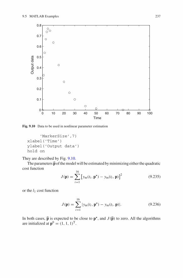
9.5 MATLAB Examples 237

0 10 20 30 40 50 60 70 80 90 1000

0.1

0.2

0.3

0.4

0.5

0.6

0.7

0.8

Time

Out

put d

ata

Fig. 9.10 Data to be used in nonlinear parameter estimation

’MarkerSize’,7)xlabel(’Time’)ylabel(’Output data’)hold on

They are described by Fig. 9.10.The parameters p of the model will be estimated by minimizing either the quadratic

cost function

J (p) =16⎡

i=1

[ym(ti , p�) − ym(ti , p)

]2 (9.235)

or the l1 cost function

J (p) =16⎡

i=1

|ym(ti , p�) − ym(ti , p)|. (9.236)

In both cases, p is expected to be close to p�, and J (p) to zero. All the algorithmsare initialized at p0 = (1, 1, 1)T.

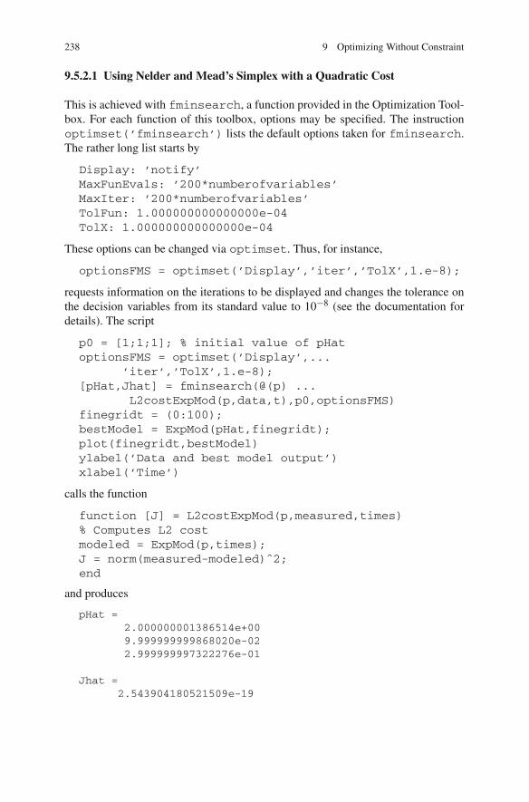
238 9 Optimizing Without Constraint

9.5.2.1 Using Nelder and Mead’s Simplex with a Quadratic Cost

This is achieved with fminsearch, a function provided in the Optimization Tool-box. For each function of this toolbox, options may be specified. The instructionoptimset(’fminsearch’) lists the default options taken for fminsearch.The rather long list starts by

Display: ’notify’MaxFunEvals: ’200*numberofvariables’MaxIter: ’200*numberofvariables’TolFun: 1.000000000000000e-04TolX: 1.000000000000000e-04

These options can be changed via optimset. Thus, for instance,

optionsFMS = optimset(’Display’,’iter’,’TolX’,1.e-8);

requests information on the iterations to be displayed and changes the tolerance onthe decision variables from its standard value to 10−8 (see the documentation fordetails). The script

p0 = [1;1;1]; % initial value of pHatoptionsFMS = optimset(’Display’,...

’iter’,’TolX’,1.e-8);[pHat,Jhat] = fminsearch(@(p) ...

L2costExpMod(p,data,t),p0,optionsFMS)finegridt = (0:100);bestModel = ExpMod(pHat,finegridt);plot(finegridt,bestModel)ylabel(’Data and best model output’)xlabel(’Time’)

calls the function

function [J] = L2costExpMod(p,measured,times)% Computes L2 costmodeled = ExpMod(p,times);J = norm(measured-modeled)ˆ2;end

and produces

pHat =2.000000001386514e+009.999999999868020e-022.999999997322276e-01

Jhat =2.543904180521509e-19

9.5 MATLAB Examples 239

0 10 20 30 40 50 60 70 80 90 1000

0.1

0.2

0.3

0.4

0.5

0.6

0.7

0.8

Time

Dat

a an

d be

st m

odel

out

put

Fig. 9.11 Least-square fit of the data in Fig. 9.10, obtained by Nelder and Mead’s simplex

after 393 evaluations of the cost function and every type of move Nelder and Mead’ssimplex algorithm can carry out.

The results of the simulation of the best model are on Fig. 9.11, together with thedata. As expected, the fit is visually perfect. Since it turns out be so with all the othermethods used to process the same data, no other such figure will be displayed.

9.5.2.2 Using Nelder and Mead’s Simplex with an l1 Cost

Nelder and Mead’s simplex can also handle nondifferentiable cost functions. Tochange the cost from l2 to l1, it suffices to replace the call to the functionL2costExpMod by a call to

function [J] = L1costExpMod(p,measured,times)% Computes L1 costmodeled = ExpMod(p,times);J = norm(measured-modeled,1)end

The optimization turns out to be a bit more difficult, though. After modifying theoptions of fminsearch according to

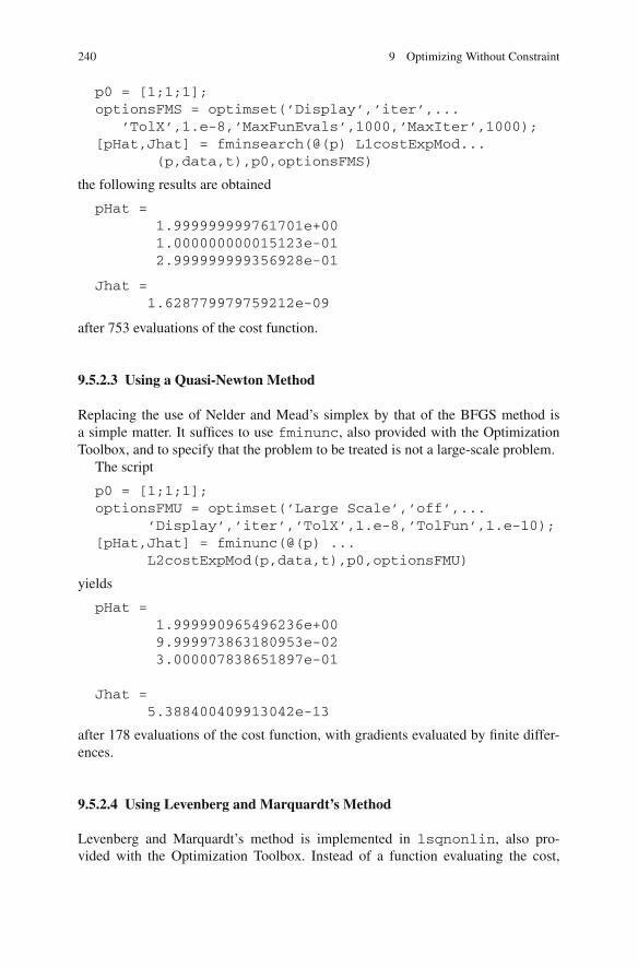
240 9 Optimizing Without Constraint

p0 = [1;1;1];optionsFMS = optimset(’Display’,’iter’,...

’TolX’,1.e-8,’MaxFunEvals’,1000,’MaxIter’,1000);[pHat,Jhat] = fminsearch(@(p) L1costExpMod...

(p,data,t),p0,optionsFMS)

the following results are obtained

pHat =1.999999999761701e+001.000000000015123e-012.999999999356928e-01

Jhat =1.628779979759212e-09

after 753 evaluations of the cost function.

9.5.2.3 Using a Quasi-Newton Method

Replacing the use of Nelder and Mead’s simplex by that of the BFGS method isa simple matter. It suffices to use fminunc, also provided with the OptimizationToolbox, and to specify that the problem to be treated is not a large-scale problem.

The script

p0 = [1;1;1];optionsFMU = optimset(’Large Scale’,’off’,...

’Display’,’iter’,’TolX’,1.e-8,’TolFun’,1.e-10);[pHat,Jhat] = fminunc(@(p) ...

L2costExpMod(p,data,t),p0,optionsFMU)

yields

pHat =1.999990965496236e+009.999973863180953e-023.000007838651897e-01

Jhat =5.388400409913042e-13

after 178 evaluations of the cost function, with gradients evaluated by finite differ-ences.

9.5.2.4 Using Levenberg and Marquardt’s Method

Levenberg and Marquardt’s method is implemented in lsqnonlin, also pro-vided with the Optimization Toolbox. Instead of a function evaluating the cost,

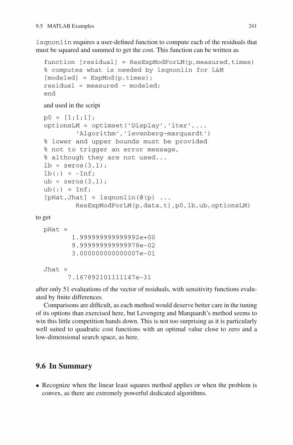
9.5 MATLAB Examples 241

lsqnonlin requires a user-defined function to compute each of the residuals thatmust be squared and summed to get the cost. This function can be written as

function [residual] = ResExpModForLM(p,measured,times)% computes what is needed by lsqnonlin for L&M[modeled] = ExpMod(p,times);residual = measured - modeled;end

and used in the script

p0 = [1;1;1];optionsLM = optimset(’Display’,’iter’,...

’Algorithm’,’levenberg-marquardt’)% lower and upper bounds must be provided% not to trigger an error message,% although they are not used...lb = zeros(3,1);lb(:) = -Inf;ub = zeros(3,1);ub(:) = Inf;[pHat,Jhat] = lsqnonlin(@(p) ...

ResExpModForLM(p,data,t),p0,lb,ub,optionsLM)

to get

pHat =1.999999999999992e+009.999999999999978e-023.000000000000007e-01

Jhat =7.167892101111147e-31

after only 51 evaluations of the vector of residuals, with sensitivity functions evalu-ated by finite differences.

Comparisons are difficult, as each method would deserve better care in the tuningof its options than exercised here, but Levengerg and Marquardt’s method seems towin this little competition hands down. This is not too surprising as it is particularlywell suited to quadratic cost functions with an optimal value close to zero and alow-dimensional search space, as here.

9.6 In Summary

• Recognize when the linear least squares method applies or when the problem isconvex, as there are extremely powerful dedicated algorithms.

242 9 Optimizing Without Constraint

• When the linear least squares method applies, avoid solving the normal equations,which may be numerically disastrous because of the computation of FTF, unlesssome very specific conditions are met. Prefer, in general, the approach based on aQR factorization or SVD of F. SVD provides the value of the condition numberof the problem for the spectral norm as a byproduct and allows ill-conditionedproblems to be regularized, but is more complex than QR factorization and doesnot necessarily give more accurate results.

• When the linear least-squares method does not apply, most of the methods pre-sented are iterative and local. They converge at best to a local minimizer, withno guarantee that it is global and unique (unless additional properties of the costfunction are known, such as convexity). When the time needed for a single localoptimization allows, multistart may be used in an attempt to escape the possibleattraction of parasitic local minimizers. This a first and particularly simple exampleof global optimization by random search, with no guarantee of success either.

• Combining line searches should be done carefully, as limiting the search directionsto fixed subspaces may forbid convergence to a minimizer.

• All the iterative methods based on Taylor expansion are not equal. The best onesstart as gradient methods and finish as Newton methods. This is the case of thequasi-Newton and conjugate-gradient methods.

• When the cost function is quadratic in some error, the Gauss-Newton method hassignificant advantages over the Newton method. It is particularly efficient whenthe minimum of the cost function is close to zero.

• Conjugate-gradient methods may be preferred over quasi-Newton methods whenthere are many decision variables. The price to be paid for this choice is that noestimate of the inverse of the Hessian at the minimizer will be provided.

• Unless the cost function is differentiable everywhere, all the local methods basedon a Taylor expansion are bound to fail. The Nelder and Mead method, whichrelies only on evaluations of the cost function is thus particularly interesting fornondifferentiable problems such as the minimization of a sum of absolute errors.

• Robust optimization makes it possible to protect oneself against the effect of factorsthat are not under control.

• Branch-and-bound methods allow statements to be proven about the global mini-mum and global minimizers.

• When the budget for evaluating the cost function is severely limited, one maytry Efficient Global Optimization (EGO), based on the use of a surrogate modelobtained by Kriging.

• The shape of the Pareto front may help one select the most appropriate tradeoffwhen objectives are conflicting.

References 243

References

1. Santner, T., Williams, B., Notz, W.: The Design and Analysis of Computer Experiments.Springer, New York (2003)

2. Lawson, C., Hanson, R.: Solving Least Squares Problems. Classics in Applied Mathematics.SIAM, Philadelphia (1995)

3. Björck, A.: Numerical Methods for Least Squares Problems. SIAM, Philadelphia (1996)4. Nievergelt, Y.: A tutorial history of least squares with applications to astronomy and geodesy.

J. Comput. Appl. Math. 121, 37–72 (2000)5. Golub, G., Van Loan, C.: Matrix Computations, 3rd edn. The Johns Hopkins University Press,

Baltimore (1996)6. Golub, G., Kahan, W.: Calculating the singular values and pseudo-inverse of a matrix. J. Soc.

Indust. Appl. Math. B. Numer. Anal. 2(2), 205–224 (1965)7. Golub, G., Reinsch, C.: Singular value decomposition and least squares solution. Numer. Math.

14, 403–420 (1970)8. Demmel, J.: Applied Numerical Linear Algebra. SIAM, Philadelphia (1997)9. Demmel, J., Kahan, W.: Accurate singular values of bidiagonal matrices. SIAM J. Sci. Stat.

Comput. 11(5), 873–912 (1990)10. Walter, E., Pronzato, L.: Identification of Parametric Models. Springer, London (1997)11. Nocedal, J., Wright, S.: Numerical Optimization. Springer, New York (1999)12. Brent, R.: Algorithms for Minimization Without Derivatives. Prentice-Hall, Englewood Cliffs

(1973)13. Press, W., Flannery, B., Teukolsky, S., Vetterling, W.: Numerical Recipes. Cambridge Univer-

sity Press, Cambridge (1986)14. Gill, P., Murray, W., Wright, M.: Practical Optimization. Elsevier, London (1986)15. Bonnans, J., Gilbert, J.C., Lemaréchal, C., Sagastizabal, C.: Numerical Optimization—

Theoretical and Practical Aspects. Springer, Berlin (2006)16. Polak, E.: Optimization—Algorithms and Consistent Approximations. Springer, New York

(1997)17. Levenberg, K.: A method for the solution of certain non-linear problems in least squares. Quart.

Appl. Math. 2, 164–168 (1944)18. Marquardt, D.: An algorithm for least-squares estimation of nonlinear parameters. J. Soc.

Indust. Appl. Math. 11(2), 431–441 (1963)19. Dennis Jr, J., Moré, J.: Quasi-Newton methods, motivations and theory. SIAM Rev. 19(1),

46–89 (1977)20. Broyden, C.: Quasi-Newton methods and their application to function minimization. Math.

Comput. 21(99), 368–381 (1967)21. Dixon, L.: Quasi Newton techniques generate identical points II: the proofs of four new theo-

rems. Math. Program. 3, 345–358 (1972)22. Gertz, E.: A quasi-Newton trust-region method. Math. Program. 100(3), 447–470 (2004)23. Shewchuk, J.: An introduction to the conjugate gradient method without the agonizing pain.

School of Computer Science, Carnegie Mellon University, Pittsburgh, Technical report (1994)24. Hager, W., Zhang, H.: A survey of nonlinear conjugate gradient methods. Pacific J. Optim.

2(1), 35–58 (2006)25. Polak, E.: Computational Methods in Optimization. Academic Press, New York (1971)26. Minoux, M.: Mathematical Programming—Theory and Algorithms. Wiley, New York (1986)27. Shor, N.: Minimization Methods for Non-differentiable Functions. Springer, Berlin (1985)28. Bertsekas, D.: Nonlinear Programming. Athena Scientific, Belmont (1999)29. Nesterov, Y.: Primal-dual subgradient methods for convex problems. Math. Program. B 120,

221–259 (2009)30. Walters, F., Parker, L., Morgan, S., Deming, S.: Sequential Simplex Optimization. CRC Press,

Boca Raton (1991)31. Lagarias, J., Reeds, J., Wright, M., Wright, P.: Convergence properties of the Nelder-Mead

simplex method in low dimensions. SIAM J. Optim. 9(1), 112–147 (1998)

244 9 Optimizing Without Constraint

32. Lagarias, J., Poonen, B., Wright, M.: Convergence of the restricted Nelder-Mead algorithm intwo dimensions. SIAM J. Optim. 22(2), 501–532 (2012)

33. Ben-Tal, A., El Ghaoui, L., Nemirovski, A.: Robust Optimization. Princeton University Press,Princeton (2009)

34. Bertsimas, D., Brown, D., Caramanis, C.: Theory and applications of robust optimization.SIAM Rev. 53(3), 464–501 (2011)

35. Le Roux, N., Schmidt, M., Bach, F.: A stochastic gradient method with an exponential con-vegence rate for strongly-convex optimization with finite training sets. In: Neural InformationProcessing Systems (NIPS 2012). Lake Tahoe (2012)

36. Rustem, B., Howe, M.: Algorithms for Worst-Case Design and Applications to Risk Manage-ment. Princeton University Press, Princeton (2002)

37. Shimizu, K., Aiyoshi, E.: Necessary conditions for min-max problems and algorithms by arelaxation procedure. IEEE Trans. Autom. Control AC-25(1), 62–66 (1980)

38. Horst, R., Tuy, H.: Global Optimization. Springer, Berlin (1990)39. Pronzato, L., Walter, E.: Eliminating suboptimal local minimizers in nonlinear parameter esti-

mation. Technometrics 43(4), 434–442 (2001)40. Whitley, L. (ed.): Foundations of Genetic Algorithms 2. Morgan Kaufmann, San Mateo (1993)41. Goldberg, D.: Genetic Algorithms in Search. Optimization and Machine Learning. Addison-

Wesley, Reading (1989)42. Storn, R., Price, K.: Differential evolution—a simple and efficient heuristic for global opti-

mization over continuous spaces. J. Global Optim. 11, 341–359 (1997)43. Dorigo, M., Stützle, T.: Ant Colony Optimization. MIT Press, Cambridge (2004)44. Kennedy, J., Eberhart, R., Shi, Y.: Swarm Intelligence. Morgan Kaufmann, San Francisco

(2001)45. Bekey, G., Masri, S.: Random search techniques for optimization of nonlinear systems with

many parameters. Math. Comput. Simul. 25, 210–213 (1983)46. Pronzato, L., Walter, E., Venot, A., Lebruchec, J.F.: A general purpose global optimizer: imple-

mentation and applications. Math. Comput. Simul. 26, 412–422 (1984)47. Jaulin, L., Kieffer, M., Didrit, O., Walter, E.: Applied Interval Analysis. Springer, London

(2001)48. Neumaier, A.: Interval Methods for Systems of Equations. Cambridge University Press,

Cambridge (1990)49. Rump, S.: INTLAB—INTerval LABoratory. In: T. Csendes (ed.) Developments in Reliable

Computing, pp. 77–104. Kluwer Academic Publishers, Dordrecht (1999)50. Rump, S.: Verification methods: rigorous results using floating-point arithmetic. Acta Numer-

ica, 287–449 (2010)51. Hansen, E.: Global Optimization Using Interval Analysis. Marcel Dekker, New York (1992)52. Kearfott, R.: Globsol user guide. Optim. Methods Softw. 24(4–5), 687–708 (2009)53. Ratschek, H., Rokne, J.: New Computer Methods for Global Optimization. Ellis Horwood,

Chichester (1988)54. Jones, D., Schonlau, M., Welch, W.: Efficient global optimization of expensive black-box

functions. J. Global Optim. 13(4), 455–492 (1998)55. Mockus, J.: Bayesian Approach to Global Optimization. Kluwer, Dordrecht (1989)56. Jones, D.: A taxonomy of global optimization methods based on response surfaces. J. Global

Optim. 21, 345–383 (2001)57. Marzat, J., Walter, E., Piet-Lahanier, H.: Worst-case global optimization of black-box functions

through Kriging and relaxation. J. Global Optim. 55(4), 707–727 (2013)58. Collette, Y., Siarry, P.: Multiobjective Optimization. Springer, Berlin (2003)

Chapter 10Optimizing Under Constraints

10.1 Introduction

Many optimization problems become meaningless unless constraints are taken intoaccount. This chapter presents techniques that can be used for this purpose. Moreinformation can be found in monographs such as [1–3]. The interior-point revolutionprovides a unifying point of view, nicely documented in [4].

10.1.1 Topographical Analogy

Assume one wants to minimize one’s altitude J (x), where x specifies one’s longitudex1 and latitude x2. Walking on a given zero-width path translates into the equalityconstraint

ce(x) = 0, (10.1)

whereas staying on a given patch of land translates into a set of inequality constraints

ci(x) � 0. (10.2)

In both cases, the neighborhood of the location with minimum altitude may not behorizontal, i.e., the gradient of J (·) may not be zero at any local or global minimizer.The optimality conditions and resulting optimization methods thus differ from thoseof the unconstrained case.

10.1.2 Motivations

A first motivation for introducing constraints on the decision vector x is forbiddingunrealistic values of decision variables. If, for instance, the i th parameter of a modelto be estimated from experimental data is the mass of a human being, one may take

É. Walter, Numerical Methods and Optimization, 245DOI: 10.1007/978-3-319-07671-3_10,© Springer International Publishing Switzerland 2014

246 10 Optimizing Under Constraints

0 � xi � 300 Kg. (10.3)

Here, the minimizer of the cost function should not be on the boundary of the feasibledomain, so none of these two inequality constraints should be active, except may betemporarily during search. They thus play no fundamental role, and are mainly usedto check a posteriori that the estimates found for the parameters are not absurd. Ifxi obtained by unconstrained minimization turns out not to belong to [0, 300] Kg,then forcing it to belong to this interval may result into xi = 0 Kg or xi = 300 Kg,neither of which might be considered satisfactory.

A second motivation is the necessity of taking into account specifications, whichusually consist of constraints, for instance in the computer-aided design of industrialproducts or in process control. Some inequality constraints are often saturated at theoptimum and would be violated unless explicitly taken into account. The constraintsmay be on quantities that depend on x, so checking that a given x belongs to X mayrequire the simulation of a numerical model.

A third motivation is dealing with conflicting objectives, by optimizing one ofthem under constraints on the others. One may, for instance, minimize the cost ofa space launcher under constraints on its payload, or maximize its payload underconstraints on its cost.

Remark 10.1 In the context of design, constraints are so crucial that the role of thecost function may even become secondary, as a way to choose a point solution xin X as defined by the constraints. One may, for instance, maximize the Euclideandistance between x in X and the closest point of the boundary ∂X of X. This ensuressome robustness to fluctuation in mass production of characteristics of componentsof the system being designed. �

Remark 10.2 Even if an unconstrained minimizer is strictly inside X, it may not beoptimal for the constrained problem, as shown by Fig. 10.1. �

10.1.3 Desirable Properties of the Feasible Set

The feasible set X defined by the constraints should of course contain several ele-ments for optimization to be possible. While checking this is easy on small academicexamples, it becomes a difficult challenge in large-scale industrial problems, whereX may turn out to be empty and one may have to relax constraints.

X is assumed here to be compact, i.e., closed and bounded. It is closed if itcontains its boundary, which forbids strict inequality constraints; it is bounded if itis impossible to make the norm of a vector x √ X tend to infinity. If the cost functionJ (·) is continuous on X and X is compact, then Weierstrass’ Theorem guarantees theexistence of a global minimizer of J (·) on X. Figure 10.2 shows a situation wherethe lack of compactness results in the absence of a minimizer.

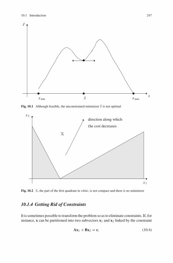
10.1 Introduction 247

J

xmin x xmaxx

Fig. 10.1 Although feasible, the unconstrained minimizer x is not optimal

direction along which

the cost decreases

x 2

x 1

Fig. 10.2 X, the part of the first quadrant in white, is not compact and there is no minimizer

10.1.4 Getting Rid of Constraints

It is sometimes possible to transform the problem so as to eliminate constraints. If, forinstance, x can be partitioned into two subvectors x1 and x2 linked by the constraint

Ax1 + Bx2 = c, (10.4)

248 10 Optimizing Under Constraints

with A invertible, then one may express x1 as a function of x2

x1 = A−1(c − Bx2). (10.5)

This decreases the dimension of search space and eliminates the need to take theconstraint (10.4) into consideration. It may, however, have negative consequenceson the structure of some of the equations to be solved by making them less sparse.

A change of variable may make it possible to eliminate inequality constraints. Toenforce the constraint xi > 0, for instance, it suffices to replace xi by exp qi , and theconstraints a < xi < b can be enforced by taking

xi = a + b

2+ b − a

2tanh qi . (10.6)

When such transformations are either impossible or undesirable, the algorithms andtheoretical optimality conditions must take the constraints into account.

Remark 10.3 When there is a mixture of linear and nonlinear constraints, it is often agood idea to treat the linear constraints separately, to take advantage of linear algebra;see Chap. 5 of [5]. �

10.2 Theoretical Optimality Conditions

Just as with unconstrained optimization, theoretical optimality conditions are usedto derive optimization methods and stopping criteria. The following difference isimportant to recall.

Contrary to what holds true in unconstrained optimization, the gradient of thecost function may not be equal to the zero vector at a minimizer. Specificoptimality conditions have thus to be derived.

10.2.1 Equality Constraints

Assume first thatX = ⎡

x : ce(x) = 0⎢, (10.7)

where the number of scalar equality constraints is ne = dim ce(x). It is important tonote that the equality constraints should be written in the standard form prescribedby (10.7) for the results to be derived to hold true. The constraint

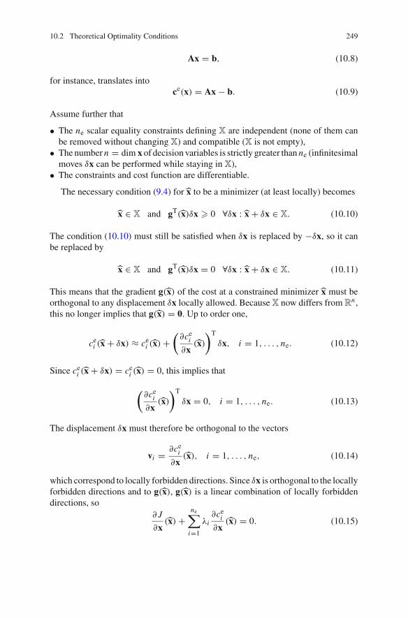
10.2 Theoretical Optimality Conditions 249

Ax = b, (10.8)

for instance, translates intoce(x) = Ax − b. (10.9)

Assume further that

• The ne scalar equality constraints defining X are independent (none of them canbe removed without changing X) and compatible (X is not empty),

• The number n = dim x of decision variables is strictly greater than ne (infinitesimalmoves δx can be performed while staying in X),

• The constraints and cost function are differentiable.

The necessary condition (9.4) for x to be a minimizer (at least locally) becomes

x √ X and gT(x)δx � 0 ∇δx : x + δx √ X. (10.10)

The condition (10.10) must still be satisfied when δx is replaced by −δx, so it canbe replaced by

x √ X and gT(x)δx = 0 ∇δx : x + δx √ X. (10.11)

This means that the gradient g(x) of the cost at a constrained minimizer x must beorthogonal to any displacement δx locally allowed. Because X now differs from R

n ,this no longer implies that g(x) = 0. Up to order one,

cei (x + δx) → ce

i (x) +⎣

∂cei

∂x(x)

⎤T

δx, i = 1, . . . , ne. (10.12)

Since cei (x + δx) = ce

i (x) = 0, this implies that

⎣∂ce

i

∂x(x)

⎤T

δx = 0, i = 1, . . . , ne. (10.13)

The displacement δx must therefore be orthogonal to the vectors

vi = ∂cei

∂x(x), i = 1, . . . , ne, (10.14)

which correspond to locally forbidden directions. Since δx is orthogonal to the locallyforbidden directions and to g(x), g(x) is a linear combination of locally forbiddendirections, so

∂ J

∂x(x) +

ne⎥

i=1

λi∂ce

i

∂x(x) = 0. (10.15)

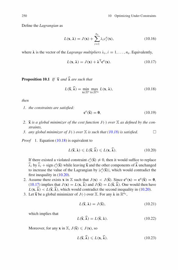
250 10 Optimizing Under Constraints

Define the Lagrangian as

L(x,λ) = J (x) +ne⎥

i=1

λi cei (x), (10.16)

where λ is the vector of the Lagrange multipliers λi , i = 1, . . . , ne. Equivalently,

L(x,λ) = J (x) + λTce(x). (10.17)

Proposition 10.1 If x and λ are such that

L (x, λ) = minx√Rn

maxλ√Rne

L(x,λ), (10.18)

then

1. the constraints are satisfied:ce (x) = 0, (10.19)

2. x is a global minimizer of the cost function J (·) over X as defined by the con-straints,

3. any global minimizer of J (·) over X is such that (10.18) is satisfied. �

Proof 1. Equation (10.18) is equivalent to

L (x,λ) � L (x, λ) � L(x, λ). (10.20)

If there existed a violated constraint cei (x) ⇒= 0, then it would suffice to replace

λi by λi + sign cei (x) while leaving x and the other components of λ unchanged

to increase the value of the Lagrangian by |cei (x)|, which would contradict the

first inequality in (10.20).2. Assume there exists x in X such that J (x) < J (x). Since ce(x) = ce(x) = 0,

(10.17) implies that J (x) = L(x, λ) and J (x) = L (x, λ). One would then haveL(x, λ) < L (x, λ), which would contradict the second inequality in (10.20).

3. Let x be a global minimizer of J (·) over X. For any λ in Rne ,

L (x,λ) = J (x), (10.21)

which implies thatL (x, λ) = L (x,λ). (10.22)

Moreover, for any x in X, J (x) � J (x), so

L (x, λ) � L(x, λ). (10.23)

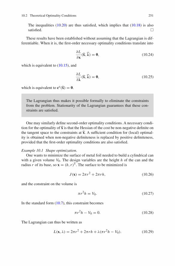
10.2 Theoretical Optimality Conditions 251

The inequalities (10.20) are thus satisfied, which implies that (10.18) is alsosatisfied. �

These results have been established without assuming that the Lagrangian is dif-ferentiable. When it is, the first-order necessary optimality conditions translate into

∂L

∂x(x, λ) = 0, (10.24)

which is equivalent to (10.15), and

∂L

∂λ(x, λ) = 0, (10.25)

which is equivalent to ce(x) = 0.

The Lagrangian thus makes it possible formally to eliminate the constraintsfrom the problem. Stationarity of the Lagrangian guarantees that these con-straints are satisfied.

One may similarly define second-order optimality conditions. A necessary condi-tion for the optimality of x is that the Hessian of the cost be non-negative definite onthe tangent space to the constraints at x. A sufficient condition for (local) optimal-ity is obtained when non-negative definiteness is replaced by positive definiteness,provided that the first-order optimality conditions are also satisfied.

Example 10.1 Shape optimization.One wants to minimize the surface of metal foil needed to build a cylindrical can

with a given volume V0. The design variables are the height h of the can and theradius r of its base, so x = (h, r)T. The surface to be minimized is

J (x) = 2πr2 + 2πrh, (10.26)

and the constraint on the volume is

πr2h = V0. (10.27)

In the standard form (10.7), this constraint becomes

πr2h − V0 = 0. (10.28)

The Lagrangian can thus be written as

L(x, λ) = 2πr2 + 2πrh + λ(πr2h − V0). (10.29)

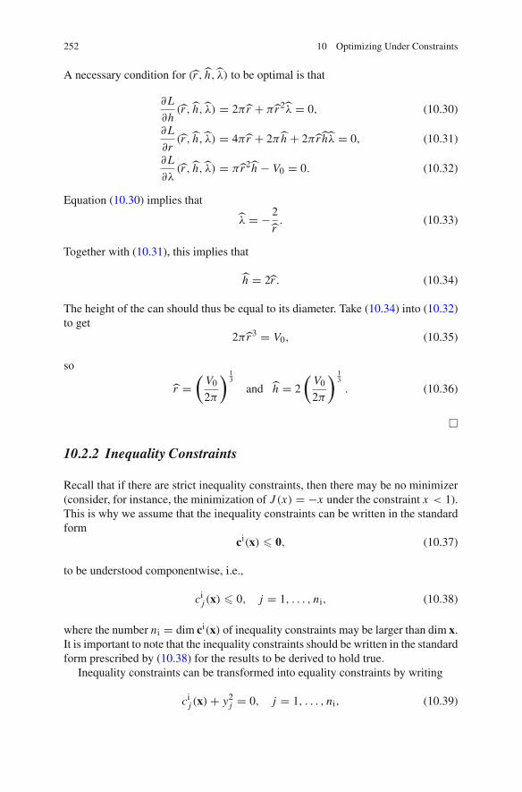
252 10 Optimizing Under Constraints

A necessary condition for (r , h, λ) to be optimal is that

∂L

∂h(r , h, λ) = 2π r + π r 2λ = 0, (10.30)

∂L

∂r(r , h, λ) = 4π r + 2π h + 2π r hλ = 0, (10.31)

∂L

∂λ(r , h, λ) = π r2h − V0 = 0. (10.32)

Equation (10.30) implies that

λ = −2

r. (10.33)

Together with (10.31), this implies that

h = 2r . (10.34)

The height of the can should thus be equal to its diameter. Take (10.34) into (10.32)to get

2π r3 = V0, (10.35)

so

r =⎣

V0

2π

⎤ 13

and h = 2

⎣V0

2π

⎤ 13

. (10.36)

�

10.2.2 Inequality Constraints

Recall that if there are strict inequality constraints, then there may be no minimizer(consider, for instance, the minimization of J (x) = −x under the constraint x < 1).This is why we assume that the inequality constraints can be written in the standardform

ci(x) � 0, (10.37)

to be understood componentwise, i.e.,

cij (x) � 0, j = 1, . . . , ni, (10.38)

where the number ni = dim ci(x) of inequality constraints may be larger than dim x.It is important to note that the inequality constraints should be written in the standardform prescribed by (10.38) for the results to be derived to hold true.

Inequality constraints can be transformed into equality constraints by writing

cij (x) + y2

j = 0, j = 1, . . . , ni, (10.39)

10.2 Theoretical Optimality Conditions 253

where y j is a slack variable, which takes the value zero when the j th scalar inequalityconstraint is active (i.e., acts as an equality constraint). When ci

j (x) = 0 , one also

says then that the j th inequality constraint is saturated or binding. (When cij (x) > 0,

the j th inequality constraint is said to be violated.)The Lagrangian associated with the equality constraints (10.39) is

L(x,μ, y) = J (x) +ni⎥

j=1

μ j

⎦ci

j (x) + y2j

⎞. (10.40)

When dealing with inequality constraints such as (10.38), the Lagrange multipliersμ j obtained in this manner are often called Kuhn and Tucker coefficients. If theconstraints and cost function are differentiable, then the first-order conditions for thestationarity of the Lagrangian are

∂L

∂x(x, μ, y) = ∂ J

∂x(x) +

ni⎥

j=1

μ j∂ci

j

∂x(x) = 0, (10.41)

∂L

∂µ j(x, μ, y) = ci

j (x) + y2j = 0, j = 1, . . . , ni, (10.42)

∂L

∂y j(x, μ, y) = 2μ j y j = 0, j = 1, . . . , ni. (10.43)

When the j th inequality constraint is inactive, y j ⇒= 0 and (10.43) implies that theassociated optimal value of the Lagrange multiplier μ j is zero. It is thus as thoughthe constraint did not exist. Condition (10.41) treats active constraints as if they wereequality constraints. As for Condition (10.42), it merely enforces the constraints.

One may also obtain second-order optimality conditions involving the Hessian ofthe Lagrangian. This Hessian is block diagonal. The block corresponding to displace-ments in the space of the slack variables is itself diagonal, with diagonal elementsgiven by

∂2L

∂y2j

= 2μ j , j = 1, . . . , ni. (10.44)

Provided J (·) is to be minimized, as assumed here, a necessary condition for opti-mality is that the Hessian be non-negative definite in the subspace authorized by theconstraints, which implies that

μ j � 0, j = 1, . . . , ni. (10.45)

Remark 10.4 Compare with equality constraints, for which there is no constraint onthe sign of the Lagrange multipliers. �

254 10 Optimizing Under Constraints

Remark 10.5 Conditions (10.45) correspond to a minimization with constraintswritten as ci(x) � 0. For a maximization or if some constraints were written asci

j (x) � 0, the conditions would differ. �

Remark 10.6 One may write the Lagrangian without introducing the slack variablesy j , provided one remembers that (10.45) should be satisfied and that μ j ci

j (x) = 0,j = 1, . . . , ni. �

All possible combinations of saturated inequality constraints must be considered,from the case where none is saturated to those where all the constraints that can besaturated at the same time are active.

Example 10.2 To minimize altitude within a square pasture X defined by fourinequality constraints, one should consider nine cases, namely

• None of these constraints is active (the minimizer may be inside the pasture),• Any one of the four constraints is active (the minimizer may be on one of the

pasture edges),• Any one of the four pairs of compatible constraints is active (the minimizer may

be at one of the pasture vertices).

All candidate minimizers thus detected should finally be compared in terms of val-ues of the objective function, after checking that they belong to X. The global min-imizer(s) may be strictly inside the pasture, but the existence of a single minimizerstrictly inside the pasture would not imply that this minimizer is globally optimal. �

Example 10.3 The cost function J (x) = x21 + x2

2 is to be minimized under theconstraint x2

1 + x22 + x1x2 � 1. The Lagrangian of the problem is thus

L(x, μ) = x21 + x2

2 + μ(1 − x21 − x2

2 − x1x2). (10.46)

Necessary conditions for optimality are μ � 0 and

∂L

∂x(x, μ) = 0. (10.47)

The condition (10.47) can be written as

A(μ)x = 0, (10.48)

with

A(μ) =⎠

2(1 − μ) −μ

−μ 2(1 − μ)

]. (10.49)

The trivial solution x = 0 violates the constraint, so μ is such that det A(μ) = 0,which implies that either μ = 2 or μ = 2/3. As both possible values of the Kuhn

10.2 Theoretical Optimality Conditions 255

and Tucker coefficient are strictly positive, the inequality constraint is saturated andcan be treated as an equality constraint

x21 + x2

2 + x1x2 = 1. (10.50)

If μ = 2, then (10.48) implies that x1 = −x2 and the two solutions of (10.50) arex1 = (1,−1)T and x2 = (−1, 1)T, with J (x1) = J (x2) = 2. If μ = 2/3,then (10.48) implies that x1 = x2 and the two solutions of (10.50) are x3 =(1/

∈3, 1/

∈3)T and x4 = (−1/

∈3,−1/

∈3)T, with J (x3) = J (x4) = 2/3. There

are thus two global minimizers, x3 and x4. �

Example 10.4 Projection onto a slabWe want to project some numerically known vector p √ R

n onto the set

S = {v √ Rn : −b � y − fTv � b}, (10.51)

where y √ R, b √ R+ and f √ R

n are known numerically. S is the slab between thehyperplanes H+ and H

− in Rn described by the equations

H+ = {v : y − fTv = b}, (10.52)

H− = {v : y − fTv = −b}. (10.53)

(H+ and H− are both orthogonal to f , so they are parallel.) This operation is at the

core of the approach for sparse estimation described in Sect. 16.27, see also [6].The result x of the projection onto S can be computed as

x = arg minx√S

‖x − p‖22. (10.54)

The Lagrangian of the problem is thus

L(x,μ) = (x − p)T(x − p) + μ1(y − fTx − b) + μ2(−y + fTx − b). (10.55)

When p is inside S, the optimal solution is of course x = p, and both Kuhn andTucker coefficients are equal to zero. When p does not belong to S, only one of theinequality constraints is violated and the projection will make this constraint active.Assume, for instance, that the constraint

y − fTp � b (10.56)

is violated. The Lagrangian then simplifies into

L(x, μ1) = (x − p)T(x − p) + μ1(y − fTx − b). (10.57)

The first-order conditions for its stationarity are

256 10 Optimizing Under Constraints

∂L

∂x(x, μ1) = 0 = 2(x − p) − μ1f, (10.58)

∂L

∂μ1(x, μ1) = 0 = y − fTx − b. (10.59)

The unique solution for μ1 and x of this system of linear equations is

μ1 = 2

⎣y − fTp − b

fTf

⎤, (10.60)

x = p + ffTf

(y − fTp − b), (10.61)

and μ1 is positive, as it should. �

10.2.3 General Case: The KKT Conditions

Assume now that J (x) must be minimized under ce(x) = 0 and ci(x) � 0. TheLagrangian can then be written as

L(x,λ,μ) = J (x) + λTce(x) + μTci(x), (10.62)

and each optimal Kuhn and Tucker coefficient μ j must satisfy μ j cij (x) = 0 and

μ j � 0. Necessary optimality conditions can be summarized in what is known asthe Karush, Kuhn, and Tucker conditions (KKT):

∂L

∂x(x, λ, μ) = ∂ J

∂x(x) +

ne⎥

i=1

λi∂ce

j

∂x(x) +

ni⎥

j=1

μ j∂ci

j

∂x(x) = 0, (10.63)

ce(x) = 0, ci(x) � 0, (10.64)

μ � 0, μ j cij (x) = 0, j = 1, . . . , ni. (10.65)

No more than dim x independent constraints can be active for any given valueof x. (The active constraints are the equality constraints and saturated inequalityconstraints.)

10.3 Solving the KKT Equations with Newton’s Method

An exhaustive formal search for all the points in decision space that satisfy the KKTconditions is only possible for relatively simple, academic problems, so numericalcomputation is usually employed instead. For each possible combination of active

10.3 Solving the KKT Equations with Newton’s Method 257

constraints, the KKT conditions boil down to a set of nonlinear equations, which maybe solved using the (damped) Newton method before checking whether the solutionthus computed belongs to X and whether the sign conditions on the Kuhn and Tuckercoefficients are satisfied. Recall, however, that

• satisfaction of the KKT conditions does not guarantee that a minimizer has beenreached,

• even if a minimizer has been found, search has only been local, so multistart mayremain in order.

10.4 Using Penalty or Barrier Functions

The simplest approach for dealing with constraints, at least conceptually, is viapenalty or barrier functions.

Penalty functions modify the cost function J (·) so as to translate constraint vio-lation into cost increase. It is then possible to fall back on classical methods forunconstrained minimization. The initial cost function may, for instance, be replacedby

Jα(x) = J (x) + αp(x), (10.66)

whereα is some positive coefficient (to be chosen by the user) and the penalty functionp(x) increases with the severity of constraint violation. One may also employ severalpenalty functions with different multiplicative coefficients. Although Jα(x) bearssome similarity with a Lagrangian, α is not optimized here.

Barrier functions also use (10.66), or a variant of it, but with p(x) increasedas soon as x approaches the boundary ∂X of X from the inside, i.e., before anyconstraint violation (barrier functions can deal with inequality constraints, providedthat the interior of X is not empty, but not with equality constraints).

10.4.1 Penalty Functions

With penalty functions, p(x) is zero as long as x belongs to X but increases withconstraint violation. For ne equality constraints, one may take, for instance, an l2penalty function

p1(x) =ne⎥

i=1

[cei (x)]2, (10.67)

or an l1 penalty function

p2(x) =ne⎥

i=1

|cei (x)|. (10.68)

258 10 Optimizing Under Constraints

For ni inequality constraints, these penalty functions would become

p3(x) =ni⎥

j=1

[max{0, cij (x)}]2, (10.69)

and

p4(x) =ni⎥

i=1

max{0, cij (x)}. (10.70)

A penalty function may be viewed as a wall around X. The greater α is in (10.66),the steeper the wall becomes, which discourages large constraint violation.

A typical strategy is to perform a series of unconstrained minimizations

xk = arg minx

Jαk (x), k = 1, 2, . . . , (10.71)

with increasing positive values of αk in order to approach ∂X from the outside. Thefinal estimate of the constrained minimizer obtained during the last minimizationserves as an initial point (or warm start) for the next.

Remark 10.7 The external iteration counter k in (10.71) should not be confusedwith the internal iteration counter of the iterative algorithm carrying out each of theminimizations. �

Under reasonable technical conditions [7, 8], there exists a finite α such that p2(·)and p4(·) yield a solution xk √ X as soon as αk > α. One then speaks of exactpenalization [1]. With p1(·) and p3(·), αk must tend to infinity to get the same result,which raises obvious numerical problems. The price to be paid for exact penalizationis that p2(·) and p4(·) are not differentiable, which complicates the minimization ofJαk (x).

Example 10.5 Consider the minimization of J (x) = x2 under the constraint x � 1.Using the penalty function p3(·), one is led to solving the unconstrained minimizationproblem

x = arg minx

Jα(x) = x2 + α[max{0, (1 − x)}]2, (10.72)

for a fixed α > 0.Since x must be positive for the constraint to be satisfied, it suffices to consider

two cases. If x > 1, then max{0, (1 − x)} = 0 and Jα(x) = x2, so the minimizer xof Jα(x) is x = 0, which is impossible. If 0 � x � 1, then max{0, (1 − x)} = 1 − xand

Jα(x) = x2 + α(1 − x)2. (10.73)

The necessary first-order optimality condition (9.6) then implies that

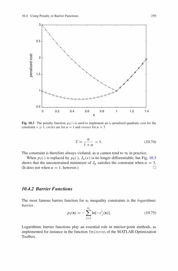
10.4 Using Penalty or Barrier Functions 259

0 0.2 0.4 0.6 0.8 1 1.2 1.4

0.5

1

1.5

2

2.5

3

x

pena

lized

cos

t

Fig. 10.3 The penalty function p4(·) is used to implement an l1-penalized quadratic cost for theconstraint x � 1; circles are for α = 1 and crosses for α = 3

x = α

1 + α< 1. (10.74)

The constraint is therefore always violated, as α cannot tend to ⊂ in practice.When p3(·) is replaced by p4(·), Jα(x) is no longer differentiable, but Fig. 10.3

shows that the unconstrained minimizer of Jα satisfies the constraint when α = 3.(It does not when α = 1, however.) �

10.4.2 Barrier Functions

The most famous barrier function for ni inequality constraints is the logarithmicbarrier.

p5(x) = −ni⎥

j=1

ln[−cij (x)]. (10.75)

Logarithmic barrier functions play an essential role in interior-point methods, asimplemented for instance in the function fmincon of the MATLAB OptimizationToolbox.

260 10 Optimizing Under Constraints

Another example of barrier function is

p6(x) = −ni⎥

j=1

1

cij (x)

. (10.76)

Since cij (x) < 0 in the interior of X, these barrier functions are well defined.

A typical strategy is to perform a series of unconstrained minimizations (10.71),with decreasing positive values of αk in order to approach ∂X from the inside. Theestimate of the constrained minimizer obtained during the last minimization againserves as an initial point for the next. This approach provides suboptimal but feasiblesolutions.

Remark 10.8 Knowledge-based models often have a limited validity domain. As aresult, the evaluation of cost functions based on such models may not make senseunless some inequality constraints are satisfied. Barrier functions are then much moreuseful for dealing with these constraints than penalty functions. �

10.4.3 Augmented Lagrangians

To avoid numerical problems resulting from too large values of α while using dif-ferentiable penalty funtions, one may add the penalty function to the Lagrangian

L(x,λ,μ) = J (x) + λTce(x) + μTci(x) (10.77)

to get the augmented Lagrangian

Lα(x,λ,μ) = L(x,λ,μ) + αp(x). (10.78)

The penalty function may be

p(x) =ne⎥

i=1

[cei (x)]2 +

ni⎥

j=1

[max{0, cij (x)]2. (10.79)

Several strategies are available for tuning x, λ and μ for a given α > 0. One of them[9] alternates

1. minimizing the augmented Lagrangian with respect to x for fixed λ and μ, bysome unconstrained optimization method,

2. performing one iteration of a gradient algorithm with step-size α for maximizingthe augmented Lagrangian with respect to λ and μ for fixed x,

10.4 Using Penalty or Barrier Functions 261

λk+1

μk+1

=

λk

μk

+ α

∂Lα

∂λ(xk,λk,μk)

∂Lα

∂μ(xk,λk,μk)

=

λk

μk

+ α

ce(xk)

ci(xk)

.

(10.80)

It is no longer necessary to make α tend to infinity to force the constraints to besatisfied exactly. Inequality constraints require special care, as only the active onesshould be taken into consideration. This corresponds to active-set strategies [3].

10.5 Sequential Quadratic Programming

In sequential quadratic programming (SQP) [10–12], the Lagrangian is approximatedby its second-order Taylor expansion in x at (xk,λk,μk), while the constraints areapproximated by their first-order Taylor expansions at xk . The KKT equations of theresulting quadratic optimization problem are then solved to get (xk+1,λk+1,μk+1),which can be done efficiently. Ideas similar to those used in the quasi-Newton meth-ods can be employed to compute approximations of the Hessian of the Laplacianbased on successive values of its gradient.

Implementing SQP, one of the most powerful approaches for nonlinear constrainedoptimization, is a complex matter best left to the specialist as SQP is availablein a number of packages. In MATLAB, one may use sqp, one of the algorithmsimplemented in the function fmincon of the MATLAB Optimization Toolbox,which is based on [13].

10.6 Linear Programming

A program (or optimization problem) is linear if the objective function and constraintsare linear (or affine) in the decision variables. Although this is a very special case, itis extremely common in practice (in economy or logistics, for instance), just as linearleast squares in the context of unconstrained optimization. Very powerful dedicatedalgorithms are available, so it is important to recognize linear programs on sight. Apedagogical introduction to linear programming is [14].

Example 10.6 Value maximizationThis is a toy example, with no pretension to economic relevance. A company

manufactures x1 metric tons of a chemical product P1 and x2 metric tons of a chemicalproduct P2. The value of a given mass of P1 is twice that of the same mass of P2and the volume of a given mass of P1 is three times that of the same mass of P2.How should the company choose x1 and x2 to maximize the value of the stock in

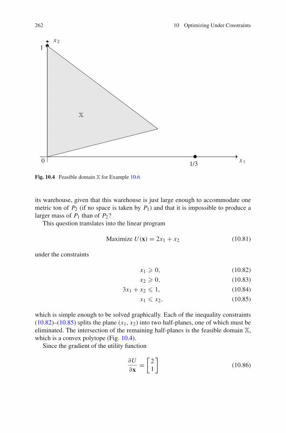
262 10 Optimizing Under Constraints

x 1

1

1/30

x 2

Fig. 10.4 Feasible domain X for Example 10.6

its warehouse, given that this warehouse is just large enough to accommodate onemetric ton of P2 (if no space is taken by P1) and that it is impossible to produce alarger mass of P1 than of P2?

This question translates into the linear program

Maximize U (x) = 2x1 + x2 (10.81)

under the constraints

x1 � 0, (10.82)

x2 � 0, (10.83)

3x1 + x2 � 1, (10.84)

x1 � x2, (10.85)

which is simple enough to be solved graphically. Each of the inequality constraints(10.82)–(10.85) splits the plane (x1, x2) into two half-planes, one of which must beeliminated. The intersection of the remaining half-planes is the feasible domain X,which is a convex polytope (Fig. 10.4).

Since the gradient of the utility function

∂U

∂x=

⎠21

](10.86)

10.6 Linear Programming 263

is never zero, there is no stationary point, and any maximizer of U (·) must belong to∂X. Now, the straight line

2x1 + x2 = a (10.87)

corresponds to all the x’s associated with the same value a of the utility function U (x).The constrained maximizer of the utility function is thus the vertex of X located onthe straight line (10.87) associated with the largest value of a, i.e.,

x = [0 1]T . (10.88)

The company should thus produce P2 only. The resulting utility is U (x) = 1. �

Example 10.7 lp-estimation for p = 1 or p = ⊂The least-squares (or l2) estimator of Sect. 9.2 is

xLS = arg minx

‖e(x)‖22, (10.89)

where the error e(x) is the N -dimensional vector of the residuals between the dataand model outputs

e(x) = y − Fx. (10.90)

When some of the data points yi are widely off the mark, for instance as a result ofsensor failure, these data points (called outliers) may affect the numerical value ofthe estimate xLS so much that it becomes useless. Robust estimators are designed tobe less sensitive to outliers. One of them is the least-modulus (or l1) estimator

xLM = arg minx

‖e(x)‖1. (10.91)

Because the components of the error vector are not squared as in the l2 estimator,the impact of a few outliers is much less drastic. The least-modulus estimator can becomputed [15, 16] as

xLM = arg minx

N⎥

i=1

(ui + vi ) (10.92)

under the constraints

ui − vi = yi − fTi x,

ui � 0, (10.93)

vi � 0.

for i = 1, . . . , N , with fTi the i th row of F. Computing xLM has thus been translated

into a linear program, where the (n + 2N ) decision variables are the n entries of x,and ui and vi (i = 1, . . . , N ). One could alternatively compute

264 10 Optimizing Under Constraints

xLM = arg minx

N⎥

i=1

1Ts, (10.94)

where 1 is a column vector with all its entries equal to one, under the constraints

y − Fx � s, (10.95)

−(y − Fx) � s, (10.96)

where the inequalities are to be understood componentwise, as usual. ComputingxLM is then again a linear program, with only (n + N ) decision variables, namelythe entries of x and s.

Similarly [15], the evaluation of a minimax (or l⊂) estimator

xMM = arg minx

‖e(x)‖⊂ (10.97)

translates into the linear program

xMM = arg minx

d⊂, (10.98)

under the constraints

y − Fx � 1d⊂, (10.99)

−(y − Fx) � 1d⊂, (10.100)

with (n + 1) decision variables, namely the entries of x and d⊂.The minimax estimator is even less robust to outliers than the l2 estimator, as

it minimizes the largest absolute deviation between a datum and the correspondingmodel output over all the data. Minimax optimization is mainly used in the contextof choosing design variables so as to protect oneself against the effect of uncertainenvironmental variables; see Sect. 9.4.1.2.

Many estimation and control problems usually treated via linear least squaresusing l2 norms can also be treated via linear programming using l1 norms; seeSect. 16.9. �Remark 10.9 In Example 10.7, unconstrained optimization problems are treated vialinear programming as constrained optimization problems. �Remark 10.10 Problems where decision variables can only take integer values mayalso be considered by combining linear programming with a branch-and-boundapproach. See Sect. 16.5. �

Real-life problems may contain many decision variables (it is now possible todeal with problems with millions of variables), so computing the value of the costfunction at each vertex of X is unthinkable and a systematic method of explorationis needed.

10.6 Linear Programming 265

Dantzig’s simplex method, not to be confused with the Nelder and Mead simplexof Sect. 9.3.5, explores ∂X by moving along edges of X from one vertex to the nextwhile improving the value of the objective function. It is considered first. Interior-point methods, which are sometimes more efficient, will be presented in Sect. 10.6.3.

10.6.1 Standard Form

To avoid having to consider a number of subcases depending on whether the objec-tive function is to be minimized or maximized and on whether there are inequalityconstraints or equality constraints or both, it is convenient to put the program in thefollowing standard form:

• J (·) is a cost function, to be minimized,• All the decision variables xi are non-negative, i.e., xi � 0,• All the constraints are equality constraints.

Achieving this is simple, at least conceptually. When a utility function U (·) is tobe maximized, it suffices to take J (x) = −U (x). When the sign of some decisionvariable xi is not known, xi can be replaced by the difference between two non-negative decision variables

xi = x+i − x−

i , with x+i � 0 and x−

i � 0. (10.101)

Any inequality constraint can be transformed into an equality constraint by intro-ducing an additional nonnegative decision variable. For instance,

3x1 + x2 � 1 (10.102)

translates into

3x1 + x2 + x3 = 1, (10.103)

x3 � 0, (10.104)

where x3 is a slack variable, and

3x1 + x2 � 1 (10.105)

translates into

3x1 + x2 − x3 = 1, (10.106)

x3 � 0, (10.107)

where x3 is a surplus variable.

266 10 Optimizing Under Constraints

The standard problem can thus be written, possibly after introducing additionalentries in the decision vector x, as that of finding

x = arg minx

J (x), (10.108)

where the cost function in (10.108) is a linear combination of the decision variables:

J (x) = cTx, (10.109)

under the constraints

Ax = b, (10.110)

x � 0. (10.111)

Equation (10.110) expresses m affine equality constraints between the n decisionvariables

n⎥

k=1

a j,k xk = bk, j = 1, . . . , m. (10.112)

The matrix A has thus m rows (as many as there are constraints) and n columns (asmany as there are variables).

Let us stress, once more, that the gradient of the cost is never zero, as

∂ J

∂x= c. (10.113)

Minimizing a linear cost in the absence of any constraint would thus not make sense,as one could make J (x) tend to −⊂ by making ||x|| tend to infinity in the direction−c. The situation is thus quite different from that with quadratic cost functions.

10.6.2 Principle of Dantzig’s Simplex Method

We assume that

• the constraints are compatible (so X is not empty),• rank A = m (so no constraint can be eliminated as redundant),• the number n of variables is larger than the number m of equality constraints (so

there is room for choice),• X as defined by (10.110) and (10.111) is bounded (it is a convex polytope).

These assumptions imply that the global minimum of the cost is reached at a vertexof X. There may be several global minimizers, but the simplex algorithm just looksfor one of them.

10.6 Linear Programming 267

The following proposition plays a key role [17].

Proposition 10.2 If x √ Rn is a vertex of a convex polytope X defined by m lin-

early independent equality constraints Ax = b, then x has at least (n − m) zeroentries. �

Proof A is m × n. If ai √ Rm is the i th column of A, then

Ax = b ∞≈n⎥

i=1

ai xi = b. (10.114)

Index the columns of A so that the nonzero entries of x are indexed from 1 to r . Then

r⎥

i=1

ai xi = b. (10.115)

Let us prove that the first r vectors ai are linearly independent. The proof is bycontradiction. If they were linearly dependent, then one could find a nonzero vectorα √ R

n such that αi = 0 for any i > r and

r⎥

i=1

ai (xi + εαi ) = b ∞≈ A(x + εα) = b, (10.116)

with ε = ±θ . Let θ be a real number, small enough to ensure that x + εα � 0. Onewould then have

x1 = x + θα √ X and x2 = x − θα √ X, (10.117)

so

x = x1 + x2

2(10.118)

could not be a vertex, as it would be strictly inside an edge. The first r vectors ai

are thus linearly independent. Now, since ai √ Rm , there are at most m linearly

independent ai ’s, so r � m and x √ Rn has at least (n − m) zero entries. �

A basic feasible solution is any xb √ X with at least (n − m) zero entries. Weassume in the description of the simplex method that one such xb has already beenfound.

Remark 10.11 When no basic feasible solution is available, one may be generated (atthe cost of increasing the dimension of search space) by the following procedure [17]:

1. add a different artificial variable to the left-hand side of each constraint thatcontains no slack variable (even if it contains a surplus variable),

2. solve the resulting set of constraints for the m artificial and slack variables, withall the initial and surplus variables set to zero. This is trivial: the artificial or slack

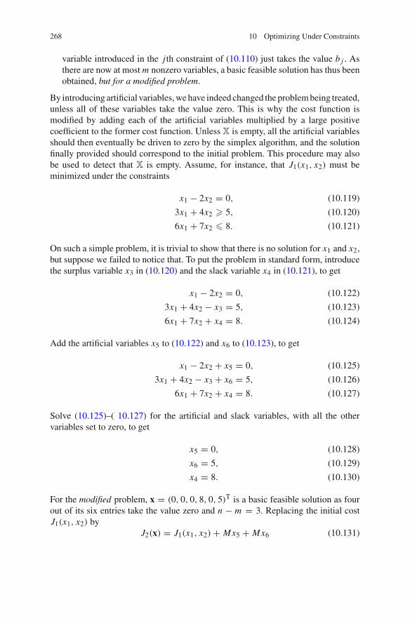
268 10 Optimizing Under Constraints

variable introduced in the j th constraint of (10.110) just takes the value b j . Asthere are now at most m nonzero variables, a basic feasible solution has thus beenobtained, but for a modified problem.

By introducing artificial variables, we have indeed changed the problem being treated,unless all of these variables take the value zero. This is why the cost function ismodified by adding each of the artificial variables multiplied by a large positivecoefficient to the former cost function. Unless X is empty, all the artificial variablesshould then eventually be driven to zero by the simplex algorithm, and the solutionfinally provided should correspond to the initial problem. This procedure may alsobe used to detect that X is empty. Assume, for instance, that J1(x1, x2) must beminimized under the constraints

x1 − 2x2 = 0, (10.119)

3x1 + 4x2 � 5, (10.120)

6x1 + 7x2 � 8. (10.121)

On such a simple problem, it is trivial to show that there is no solution for x1 and x2,but suppose we failed to notice that. To put the problem in standard form, introducethe surplus variable x3 in (10.120) and the slack variable x4 in (10.121), to get

x1 − 2x2 = 0, (10.122)

3x1 + 4x2 − x3 = 5, (10.123)

6x1 + 7x2 + x4 = 8. (10.124)

Add the artificial variables x5 to (10.122) and x6 to (10.123), to get

x1 − 2x2 + x5 = 0, (10.125)

3x1 + 4x2 − x3 + x6 = 5, (10.126)

6x1 + 7x2 + x4 = 8. (10.127)

Solve (10.125)–( 10.127) for the artificial and slack variables, with all the othervariables set to zero, to get

x5 = 0, (10.128)

x6 = 5, (10.129)

x4 = 8. (10.130)

For the modified problem, x = (0, 0, 0, 8, 0, 5)T is a basic feasible solution as fourout of its six entries take the value zero and n − m = 3. Replacing the initial costJ1(x1, x2) by

J2(x) = J1(x1, x2) + Mx5 + Mx6 (10.131)

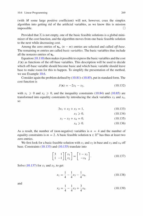
10.6 Linear Programming 269

(with M some large positive coefficient) will not, however, coax the simplexalgorithm into getting rid of the artificial variables, as we know this is missionimpossible. �

Provided that X is not empty, one of the basic feasible solutions is a global mini-mizer of the cost function, and the algorithm moves from one basic feasible solutionto the next while decreasing cost.

Among the zero entries of xb, (n − m) entries are selected and called off-base.The remaining m entries are called basic variables. The basic variables thus includeall the nonzero entries of xb.

Equation (10.110) then makes it possible to express the basic variables and the costJ (x) as functions of the off-base variables. This description will be used to decidewhich off-base variable should become basic and which basic variable should leavebase to make room for this to happen. To simplify the presentation of the method,we use Example 10.6.

Consider again the problem defined by (10.81)–(10.85), put in standard form. Thecost function is

J (x) = −2x1 − x2, (10.132)

with x1 � 0 and x2 � 0, and the inequality constraints (10.84) and (10.85) aretransformed into equality constraints by introducing the slack variables x3 and x4,so

3x1 + x2 + x3 = 1, (10.133)

x3 � 0, (10.134)

x1 − x2 + x4 = 0, (10.135)

x4 � 0. (10.136)

As a result, the number of (non-negative) variables is n = 4 and the number ofequality constraints is m = 2. A basic feasible solution x √ R

4 has thus at least twozero entries.

We first look for a basic feasible solution with x1 and x2 in base and x3 and x4 offbase. Constraints (10.133) and (10.135) translate into

⎠3 11 −1

] ⎠x1x2

]=

⎠1 − x3−x4

]. (10.137)

Solve (10.137) for x1 and x2, to get

x1 = 1

4− 1

4x3 − 1

4x4, (10.138)

and

x2 = 1

4− 1

4x3 + 3

4x4. (10.139)

270 10 Optimizing Under Constraints

Table 10.1 Initial situationin Example 10.6

Constant coefficient Coefficient of x3 Coefficient of x4

J −3/4 3/4 −1/4x1 1/4 −1/4 −1/4x2 1/4 −1/4 3/4

It is trivial to check that the vector x obtained by setting x3 and x4 to zero andchoosing x1 and x2 so as to satisfy (10.138) and (10.139), i.e.,

x =⎠

1

4

1

40 0

]T

, (10.140)

satisfies all the constraints while having an appropriate number of zero entries, andis thus a basic feasible solution.

The cost can also be expressed as a function of the off-base variables, as (10.132),(10.138) and (10.139) imply that

J (x) = −3

4+ 3

4x3 − 1

4x4. (10.141)

The situation is summarized in Table 10.1.The last two rows of the first column of Table 10.1 list the basic variables, while

the last two columns of the first row list the off-base variables. The simplex algo-rithm modifies this table iteratively, by exchanging basic and off-base variables. Themodification to be carried out during a given iteration is decided in three steps.

The first step selects, among the off-base variables, one such that the associatedentry in the cost row is

• negative (to allow the cost to decrease),• with the largest absolute value (to make this happen quickly).

In our example, only x4 is associated with a negative coefficient, so it is selected tobecome a basic variable. When there are several equally promising off-base variables(negative coefficient with maximum absolute value), an unlikely event, one may pickup one of them at random. If no off-base variable has a negative coefficient, then thecurrent basic feasible solution is globally optimal and the algorithm stops.

The second step increases the off-base variable xi selected during the first step tojoin base (in our example, i = 4), until one of the basic variables becomes equal tozero and thus leaves base to make room for xi . To discover which of the previousbasic variables will be ousted, the signs of the coefficients located at the intersectionsbetween the column associated to the new basic variable xi and the rows associated tothe previous basic variables must be considered. When these coefficient are positive,increasing xi also increases the corresponding variables, which thus stay in base.The variable due to leave base therefore has a negative coefficient. The first formerbasic variable with a negative coefficient to reach zero when xi is increased will be

10.6 Linear Programming 271

Table 10.2 Final situation inExample 10.6

Constant coefficient Coefficient of x1 Coefficient of x3

J −1 1 1x2 1 −3 −1x4 1 −4 −1

the one leaving base. In our example, there is only one negative coefficient, whichis equal to −1/4 and associated with x1. The variable x1 becomes equal to zero andleaves base when the new basic variable x4 reaches 1.

The third step updates the table. In our example, the basic variables are now x2and x4 and the off-base variables x1 and x3. It is thus necessary to express x2, x4 andJ as functions of x1 and x3. From (10.133) and (10.135), we get

x2 = 1 − 3x1 − x3, (10.142)

−x2 + x4 = −x1, (10.143)

or equivalently

x2 = 1 − 3x1 − x3, (10.144)

x4 = 1 − 4x1 − x3. (10.145)

As for the cost, (10.132) and (10.144) imply that

J (x) = −1 + x1 + x3. (10.146)

Table 10.1 thus becomes Table 10.2.All the off-base variables have now positive coefficients in the cost row. It is

therefore no longer possible to improve the current basic feasible solution

x = [0 1 0 1]T, (10.147)

which is thus (globally) optimal and associated with the lowest possible cost

J (x) = −1. (10.148)

This corresponds to an optimal utility equal to 1, consistent with the results obtainedgraphically.

10.6.3 The Interior-Point Revolution

Until 1984, Dantzig’s simplex enjoyed a near monopoly in the context of linear pro-gramming, which was seen as having little connection with nonlinear programming.

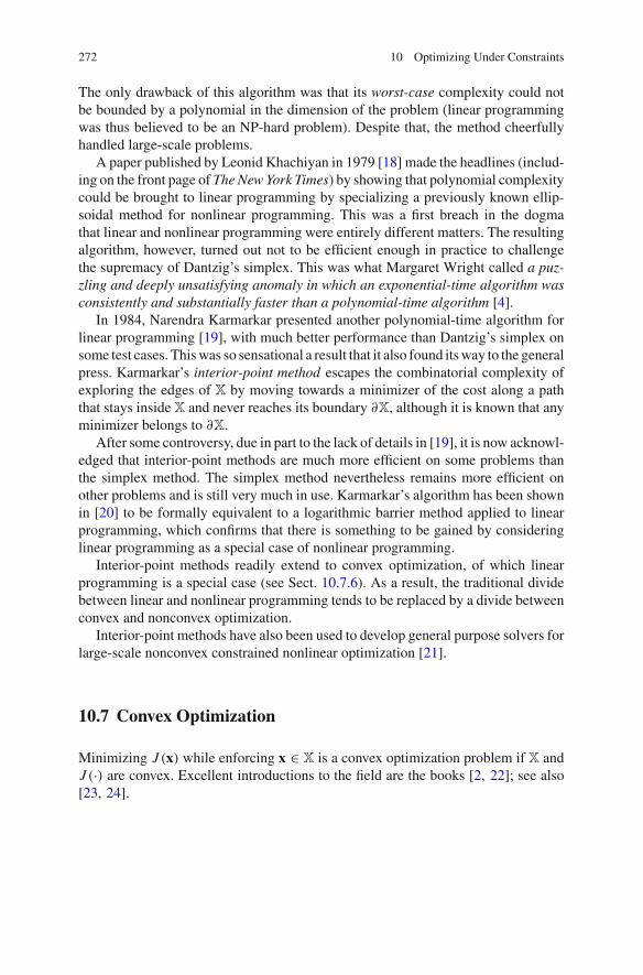
272 10 Optimizing Under Constraints

The only drawback of this algorithm was that its worst-case complexity could notbe bounded by a polynomial in the dimension of the problem (linear programmingwas thus believed to be an NP-hard problem). Despite that, the method cheerfullyhandled large-scale problems.

A paper published by Leonid Khachiyan in 1979 [18] made the headlines (includ-ing on the front page of The New York Times) by showing that polynomial complexitycould be brought to linear programming by specializing a previously known ellip-soidal method for nonlinear programming. This was a first breach in the dogmathat linear and nonlinear programming were entirely different matters. The resultingalgorithm, however, turned out not to be efficient enough in practice to challengethe supremacy of Dantzig’s simplex. This was what Margaret Wright called a puz-zling and deeply unsatisfying anomaly in which an exponential-time algorithm wasconsistently and substantially faster than a polynomial-time algorithm [4].

In 1984, Narendra Karmarkar presented another polynomial-time algorithm forlinear programming [19], with much better performance than Dantzig’s simplex onsome test cases. This was so sensational a result that it also found its way to the generalpress. Karmarkar’s interior-point method escapes the combinatorial complexity ofexploring the edges of X by moving towards a minimizer of the cost along a paththat stays inside X and never reaches its boundary ∂X, although it is known that anyminimizer belongs to ∂X.

After some controversy, due in part to the lack of details in [19], it is now acknowl-edged that interior-point methods are much more efficient on some problems thanthe simplex method. The simplex method nevertheless remains more efficient onother problems and is still very much in use. Karmarkar’s algorithm has been shownin [20] to be formally equivalent to a logarithmic barrier method applied to linearprogramming, which confirms that there is something to be gained by consideringlinear programming as a special case of nonlinear programming.

Interior-point methods readily extend to convex optimization, of which linearprogramming is a special case (see Sect. 10.7.6). As a result, the traditional dividebetween linear and nonlinear programming tends to be replaced by a divide betweenconvex and nonconvex optimization.

Interior-point methods have also been used to develop general purpose solvers forlarge-scale nonconvex constrained nonlinear optimization [21].

10.7 Convex Optimization

Minimizing J (x) while enforcing x √ X is a convex optimization problem if X andJ (·) are convex. Excellent introductions to the field are the books [2, 22]; see also[23, 24].

10.7 Convex Optimization 273

Fig. 10.5 The set on the left is convex; the one on the right is not, as the line segment joining thetwo dots is not included in the set

10.7.1 Convex Feasible Sets

The setX is convex if, for any pair (x1, x2) of points inX, the line segment connectingthese points is included in X:

∇λ √ [0, 1], λx1 + (1 − λ)x2 √ X; (10.149)

see Fig. 10.5.

Example 10.8 Rn , hyperplanes, half-spaces, ellipsoids, and unit balls for any norm

are convex, and the intersection of convex sets is convex. The feasible sets of linearprograms are thus convex. �

10.7.2 Convex Cost Functions

The function J (·) is convex on X if J (x) is defined for any x in X and if, for any pair(x1, x2) of points in X, the following inequality holds:

∇λ √ [0, 1] J (λx1 + (1 − λ)x2) � λJ (x1) + (1 − λ)J (x2); (10.150)

see Fig. 10.6.

Example 10.9 The function

J (x) = xTAx + bTx + c (10.151)

is convex, provided that A is symmetric non-negative definite. �

274 10 Optimizing Under Constraints

J1 J 2

x x

Fig. 10.6 The function on the left is convex; the one on the right is not

Example 10.10 The functionJ (x) = cTx (10.152)

is convex. Linear-programming cost functions are thus convex. �

Example 10.11 The function

J (x) =⎥

i

wi Ji (x) (10.153)

is convex if each of the functions Ji (x) is convex and each weight wi is positive. �

Example 10.12 The function

J (x) = maxi

Ji (x) (10.154)

is convex if each of the functions Ji (x) is convex. �

If a function is convex on X, then it is continuous on any open set included inX. A necessary and sufficient condition for a once-differentiable function J (·) to beconvex is that

∇x1 √ X,∇x2 √ X, J (x2) � J (x1) + gT(x1)(x2 − x1), (10.155)

10.7 Convex Optimization 275

where g(·) is the gradient function of J (·). This provides a global lower bound forthe function from the knowledge of the value of its gradient at any given point x1.

10.7.3 Theoretical Optimality Conditions

Convexity transforms the necessary first-order conditions for optimality of Sects. 9.1and 10.2 into necessary and sufficient conditions for global optimality. If J (·) isconvex and once differentiable, then a necessary and sufficient condition for x to bea global minimizer in the absence of constraint is

g(x) = 0. (10.156)

When constraints define a feasible set X, this condition becomes

gT(x)(x2 − x) � 0 ∇x2 √ X, (10.157)

a direct consequence of (10.155).

10.7.4 Lagrangian Formulation

Consider again the Lagrangian formulation of Sect. 10.2, while taking advantage ofconvexity. The Lagrangian for the minimization of the cost function J (x) under theinequality constraints ci(x) � 0 is

L(x,μ) = J (x) + μTci(x), (10.158)

where the vector μ of Lagrange (or Kuhn and Tucker) multipliers is also called thedual vector. The dual function D(μ) is the infimum of the Lagrangian over x

D(μ) = infx

L(x,μ). (10.159)

Since J (x) and all the constraints cij (x) are assumed to be convex, L(x,μ) is a convex

function of x as long as μ � 0, which must be true for inequality constraints anyway.So the evaluation of D(μ) is an unconstrained convex minimization problem, whichcan be solved with a local method such as Newton or quasi-Newton. If the infimumof L(x,μ) with respect to x is reached at xμ, then

D(μ) = J (xμ) + μTci(xμ). (10.160)

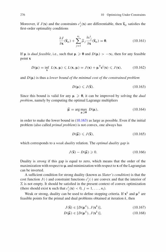
276 10 Optimizing Under Constraints

Moreover, if J (x) and the constraints cij (x) are differentiable, then xμ satisfies the

first-order optimality conditions

∂ J

∂x(xμ) +

ni⎥

j=1

μ j∂ci

j

∂x(xμ) = 0. (10.161)

If μ is dual feasible, i.e., such that μ � 0 and D(μ) > −⊂, then for any feasiblepoint x

D(μ) = infx

L(x,μ) � L(x,μ) = J (x) + μTci(x) � J (x), (10.162)

and D(μ) is thus a lower bound of the minimal cost of the constrained problem

D(μ) � J (x). (10.163)

Since this bound is valid for any μ � 0, it can be improved by solving the dualproblem, namely by computing the optimal Lagrange multipliers

μ = arg maxμ�0

D(μ), (10.164)

in order to make the lower bound in (10.163) as large as possible. Even if the initialproblem (also called primal problem) is not convex, one always has

D(μ) � J (x), (10.165)

which corresponds to a weak duality relation. The optimal duality gap is

J (x) − D(μ) � 0. (10.166)

Duality is strong if this gap is equal to zero, which means that the order of themaximization with respect to μ and minimization with respect to x of the Lagrangiancan be inverted.

A sufficient condition for strong duality (known as Slater’s condition) is that thecost function J (·) and constraint functions ci

j (·) are convex and that the interior ofX is not empty. It should be satisfied in the present context of convex optimization(there should exist x such that ci

j (x) < 0, j = 1, . . . , ni).

Weak or strong, duality can be used to define stopping criteria. If xk and μk arefeasible points for the primal and dual problems obtained at iteration k, then

J (x) √ [D(μk), J (xk)], (10.167)

D(μ) √ [D(μk), J (xk)], (10.168)

10.7 Convex Optimization 277

with the duality gap given by the width of the interval [D(μk), J (xk)]. One may stopas soon as the duality gap is deemed acceptable (in absolute or relative terms).

10.7.5 Interior-Point Methods

By solving a succession of unconstrained optimization problems, interior-point meth-ods generate sequences of pairs (xk,μk) such that

• xk is strictly inside X,• μk is strictly feasible for the dual problem (each Lagrange multiplier is strictly

positive),• the width of the interval [D(μk), J (xk)] decreases when k increases.

Under the condition of strong duality, (xk,μk) converges to the optimal solution(x, μ) when k tends to infinity, and this is true even when x belongs to ∂X.

To get a starting point x0, one may compute

(w, x0) = arg minw,x

w (10.169)

under the constraintsci

j (x) � w, j = 1, . . . , ni. (10.170)

If w < 0, then x0 is strictly inside X. If w = 0 then x0 belongs to ∂X and cannot beused for an interior-point method. If w > 0, then the initial problem has no solution.

To remain strictly insideX, one may use a barrier function, usually the logarithmicbarrier defined by (10.75), or more precisely by

plog(x) ={−∑ni

j=1 ln[−cij (x)] if ci(x) < 0,

+⊂ otherwise.(10.171)

This barrier is differentiable and convex inside X; it tends to infinity when x tends to∂X from within. One then solves the unconstrained convex minimization problem

xα = arg minx

[J (x) + αplog(x)], (10.172)

where α is a positive real coefficient to be chosen. The locus of the xα’s for α > 0 iscalled the central path, and each xα is a central point. Taking αk = 1/βk , where βk

is some increasing function of k, one can compute a sequence of central points bysolving a succession of unconstrained convex minimization problems for k = 1, 2, . . .

The central point xk is given by

xk = arg minx

[J (x) + αk plog(x)] = arg minx

[βk J (x) + plog(x)]. (10.173)

278 10 Optimizing Under Constraints

This can be done very efficiently by a Newton-type method, with a warm start atxk−1 of the search for xk . The larger βk becomes, the more xk approaches ∂X, as therelative weight of the cost with respect to the barrier increases. If J (x) and ci(x) areboth differentiable, then xk should satisfy the first-order optimality condition

βk∂ J

∂x(xk) + ∂plog

∂x(xk) = 0, (10.174)

which is necessary and sufficient as the problem is convex. An important result [2]is that

• every central point xk is feasible for the primal problem,• a feasible point for the dual problem is

μkj = − 1

βkcij (x

k)j = 1, . . . , ni, (10.175)

• and the duality gap is

J (xk) − D(μk) = ni

βk, (10.176)

with ni the number of inequality constraints.

Remark 10.12 Since xk is strictly inside X, cij (x

k) < 0 and μkj as given by (10.175)

is strictly positive. �

The duality gap thus tends to zero as βk tends to infinity, which ensures (at leastmathematically), that xk tends to an optimal solution of the primal problem when ktends to infinity.

One may take, for instance,βk = γβk−1, (10.177)

with γ > 1 and β0 > 0 to be chosen. Two types of problems may arise:

• when β0 and especially γ are too small, one will lose time crawling along thecentral path,

• when they are too large, the search for xk may be badly initialized by the warmstart and Newton’s method may lose time multiplying iterations.

10.7.6 Back to Linear Programming

MinimizingJ (x) = cTx (10.178)

under the inequality constraints

10.7 Convex Optimization 279

Ax � b (10.179)

is a convex problem, since the cost function and the feasible domain are convex. TheLagrangian is

L(x,μ) = cTx + μT(Ax − b) = −bTμ + (ATμ + c)Tx. (10.180)

The dual function is such that

D(μ) = infx

L(x,μ). (10.181)

Since the Lagrangian is affine in x, the infimum is −⊂ unless ∂L/∂x is identicallyzero, so

D(μ) ={−bTμ if ATμ + c = 0

−⊂ otherwise

and μ is dual feasible if μ � 0 and ATμ + c = 0.The use of a logarithmic barrier leads to computing the central points

xk = arg minx

Jk(x), (10.182)

where

Jk(x) = βkcTx −ni⎥

j=1

ln(b j − aTj x), (10.183)

with aTj the j th row of A. This is unconstrained convex minimization, and thus easy.

A necessary and sufficient condition for xk to be a solution of (10.182) is that

gk(xk) = 0, (10.184)

with gk(·) the gradient of Jk(·), trivial to compute as

gk(x) = ∂ Jk

∂x(x) = βkc +

ni⎥

j=1

1

b j − aTj x

a j . (10.185)

To search for xk with a (damped) Newton method, one also needs the Hessian ofJk(·), given by

Hk(x) = ∂2 Jk

∂x∂xT (x) =ni⎥

j=1

1

(b j − aTj x)2

a j aTj . (10.186)

280 10 Optimizing Under Constraints

Hk is obviously symmetrical. Provided that there are dim x linearly independentvectors a j , it is also positive definite so a damped Newton method should convergeto the unique global minimizer of (10.178) under (10.179). One may alternativelyemploy a quasi-Newton or conjugate-gradient method that only uses evaluations ofthe gradient.

Remark 10.13 The internal Newton, quasi-Newton, or conjugate-gradient methodwill have its own iteration counter, not to be confused with that of the externaliteration, denoted here by k. �

Equation (10.175) suggests taking as the dual vector associated with xk the vectorμk with entries

μkj = − 1

βkcij (x

k), j = 1, . . . , ni, (10.187)

i.e.,

μkj = 1

βk(b j − aTj xk)

, j = 1, . . . , ni. (10.188)

The duality gap

J (xk) − D(μk) = ni

βk(10.189)

may serve to decide when to stop.

10.8 Constrained Optimization on a Budget

The philosophy behind efficient global optimization (EGO) can be extended to dealwith constrained optimization where evaluating the cost function and/or the con-straints is so expensive that the number of evaluations allowed is severely limited[25, 26].

Penalty functions may be used to transform the constrained optimization probleminto an unconstrained one, to which EGO can then be applied. When constraintevaluation is expensive, this approach has the advantage of building a surrogatemodel that takes the original cost and the constraints into account. The tuning ofthe multiplicative coefficients applied to the penalty functions is not trivial in thiscontext, however.

An alternative approach is to carry out a constrained maximization of the expectedimprovement of the original cost. This is particularly interesting when the evalua-tion of the constraints is much less expensive than that of the original cost, as theconstrained maximization of the expected improvement will then be relatively inex-pensive, even if penalty functions have to be tuned.

10.9 MATLAB Examples 281

10.9 MATLAB Examples

10.9.1 Linear Programming

Three main methods for linear programming are implemented in linprog, a func-tion provided in the Optimization Toolbox:

• a primal-dual interior-point method for large-scale problems,• an active-set method (a variant of sequential quadratic programming) for medium-

scale problems,• Dantzig’s simplex for medium-scale problems.

The instruction optimset(’linprog’) lists the default options. They include

Display: ’final’Diagnostics: ’off’LargeScale: ’on’

Simplex: ’off’

Let us employ Dantzig’s simplex on Example 10.6. The function linprog assumesthat

• a linear cost is to be minimized, so we use the cost function (10.109), with

c = (−2,−1)T; (10.190)

• the inequality constraints are not transformed into equality constraints, but writtenas

Ax � b, (10.191)

so we take

A =⎠

3 11 −1

]and b =

⎠10

]; (10.192)

• any lower or upper bound on a decision variable is given explicitly, so we mustmention that the lower bound for each of the two decision variables is zero.

This is implemented in the script

clear allc = [-2;

-1];A = [3 1;

1 -1];b = [1;

0];LowerBound = zeros(2,1);% Forcing the use of Simplex

282 10 Optimizing Under Constraints

optionSIMPLEX = ...optimset(’LargeScale’,’off’,’Simplex’,’on’)

[OptimalX, OptimalCost] = ...linprog(c,A,b,[],[],LowerBound,...[],[],optionSIMPLEX)

The brackets [] in the list of input arguments of linprog correspond to argumentsnot used here, such as upper bounds on the decision variables. See the documentationof the toolbox for more details. This script yields

Optimization terminated.

OptimalX =01

OptimalCost =-1

which should come as no surprise.

10.9.2 Nonlinear Programming

The function patternsearch of the Global Optimization Toolbox makes it possi-ble to deal with a mixture of linear and nonlinear, equality and inequality constraintsusing an Augmented Lagrangian Pattern Search algorithm (ALPS) [27–29]. Linearconstraints are treated separately from the nonlinear ones.

Consider again Example 10.5. The inequality constraint is so simple that it can beimplemented by putting a lower bound on the decision variable, as in the followingscript, where all the unused arguments of patternsearch that must be providedbefore the lower bound are replaced by []

x0 = 0;Cost = @(x) x.ˆ2;LowerBound = 1;[xOpt,CostOpt] = patternsearch(Cost,x0,[],[],...

[],[], LowerBound)

The solution is found to be

xOpt = 1CostOpt = 1

as expected.

10.9 MATLAB Examples 283

Consider now Example 10.3, where the cost function J (x) = x21 + x2

2 must beminimized under the nonlinear inequality constraint x2

1 + x22 + x1x2 � 1. We know

that there are two global minimizers

x3 = (1/∈

3, 1/∈

3)T, (10.193)

x4 = (−1/∈

3,−1/∈

3)T, (10.194)

where 1/∈

3 → 0.57735026919, and that J (x3) = J (x4) = 2/3 → 0.66666666667.The cost function is implemented by the function

function Cost = L2cost(x)Cost = norm(x)ˆ2;end

The nonlinear inequality constraint is written as c(x) � 0, and implemented by thefunction

function [c,ceq] = NLConst(x)c = 1 - x(1)ˆ2 - x(2)ˆ2 - x(1)*x(2);ceq = [];end

Since there is no nonlinear equality constraint, ceq is left empty but must be present.Finally, patternsearch is called with the script

clear allx0 = [0;0];x = zeros(2,1);[xOpt,CostOpt] = patternsearch(@(x) ...

L2cost(x),x0,[],[],...[],[],[],[], @(x) NLconst(x))

which yields, after 4000 evaluations of the cost function,

Optimization terminated: mesh size lessthan options.TolMesh and constraint violationis less than options.TolCon.

xOpt =-5.672302246093750e-01-5.882263183593750e-01

CostOpt =6.677603293210268e-01

The accuracy of this solution can be slightly improved (at the cost of a major increasein computing time) by changing the options of patternsearch, as in the follow-ing script

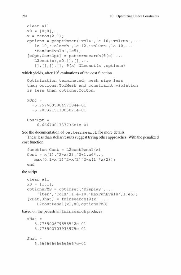
284 10 Optimizing Under Constraints

clear allx0 = [0;0];x = zeros(2,1);options = psoptimset(’TolX’,1e-10,’TolFun’,...

1e-10,’TolMesh’,1e-12,’TolCon’,1e-10,...’MaxFunEvals’,1e5);

[xOpt,CostOpt] = patternsearch(@(x) ...L2cost(x),x0,[],[],...[],[],[],[], @(x) NLconst(x),options)

which yields, after 105 evaluations of the cost function

Optimization terminated: mesh size lessthan options.TolMesh and constraint violationis less than options.TolCon.

xOpt =-5.757669508457184e-01-5.789321511983871e-01

CostOpt =6.666700173773681e-01

See the documentation of patternsearch for more details.These less than stellar results suggest trying other approaches. With the penalized

cost function

function Cost = L2costPenal(x)Cost = x(1).ˆ2+x(2).ˆ2+1.e6*...

max(0,1-x(1)ˆ2-x(2)ˆ2-x(1)*x(2));end

the script

clear allx0 = [1;1];optionsFMS = optimset(’Display’,...

’iter’,’TolX’,1.e-10,’MaxFunEvals’,1.e5);[xHat,Jhat] = fminsearch(@(x) ...

L2costPenal(x),x0,optionsFMS)

based on the pedestrian fminsearch produces

xHat =5.773502679858542e-015.773502703933975e-01

Jhat =6.666666666666667e-01

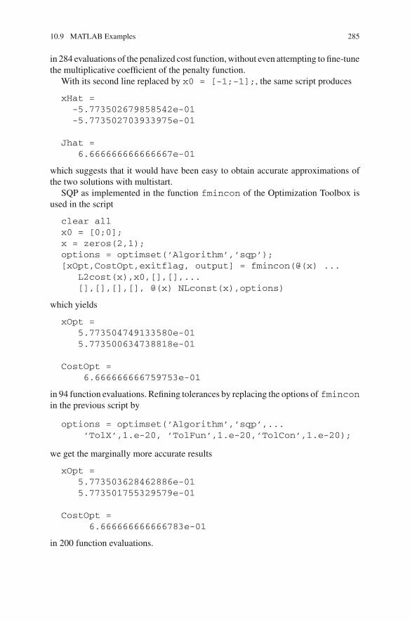
10.9 MATLAB Examples 285

in 284 evaluations of the penalized cost function, without even attempting to fine-tunethe multiplicative coefficient of the penalty function.

With its second line replaced by x0 = [-1;-1];, the same script produces

xHat =-5.773502679858542e-01-5.773502703933975e-01

Jhat =6.666666666666667e-01

which suggests that it would have been easy to obtain accurate approximations ofthe two solutions with multistart.

SQP as implemented in the function fmincon of the Optimization Toolbox isused in the script

clear allx0 = [0;0];x = zeros(2,1);options = optimset(’Algorithm’,’sqp’);[xOpt,CostOpt,exitflag, output] = fmincon(@(x) ...

L2cost(x),x0,[],[],...[],[],[],[], @(x) NLconst(x),options)

which yields

xOpt =5.773504749133580e-015.773500634738818e-01

CostOpt =6.666666666759753e-01

in 94 function evaluations. Refining tolerances by replacing the options of fminconin the previous script by

options = optimset(’Algorithm’,’sqp’,...’TolX’,1.e-20, ’TolFun’,1.e-20,’TolCon’,1.e-20);

we get the marginally more accurate results

xOpt =5.773503628462886e-015.773501755329579e-01

CostOpt =6.666666666666783e-01

in 200 function evaluations.

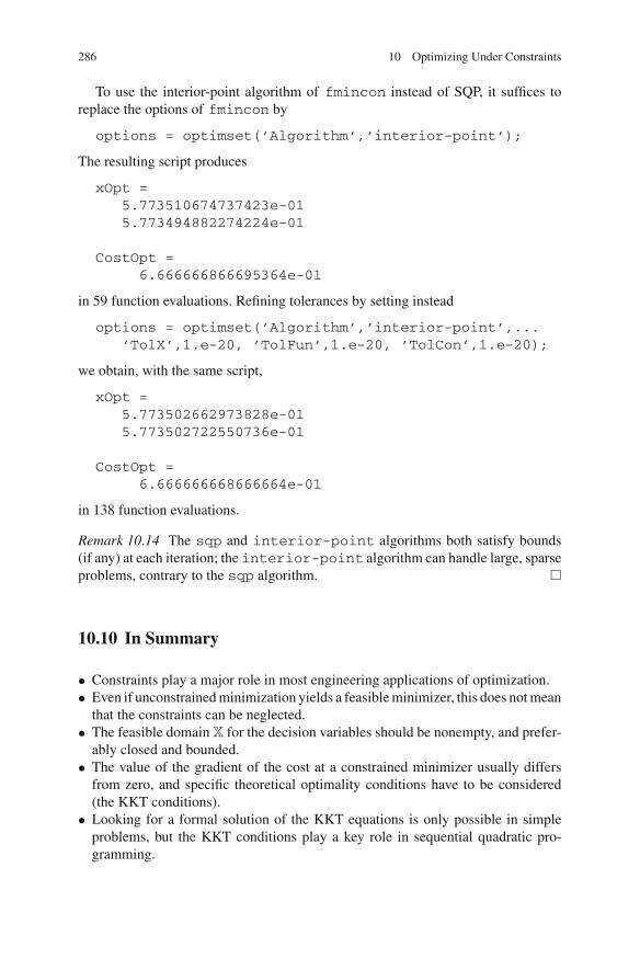
286 10 Optimizing Under Constraints

To use the interior-point algorithm of fmincon instead of SQP, it suffices toreplace the options of fmincon by

options = optimset(’Algorithm’,’interior-point’);

The resulting script produces

xOpt =5.773510674737423e-015.773494882274224e-01

CostOpt =6.666666866695364e-01

in 59 function evaluations. Refining tolerances by setting instead

options = optimset(’Algorithm’,’interior-point’,...’TolX’,1.e-20, ’TolFun’,1.e-20, ’TolCon’,1.e-20);

we obtain, with the same script,

xOpt =5.773502662973828e-015.773502722550736e-01

CostOpt =6.666666668666664e-01

in 138 function evaluations.

Remark 10.14 The sqp and interior-point algorithms both satisfy bounds(if any) at each iteration; the interior-point algorithm can handle large, sparseproblems, contrary to the sqp algorithm. �

10.10 In Summary

• Constraints play a major role in most engineering applications of optimization.• Even if unconstrained minimization yields a feasible minimizer, this does not mean

that the constraints can be neglected.• The feasible domain X for the decision variables should be nonempty, and prefer-

ably closed and bounded.• The value of the gradient of the cost at a constrained minimizer usually differs

from zero, and specific theoretical optimality conditions have to be considered(the KKT conditions).

• Looking for a formal solution of the KKT equations is only possible in simpleproblems, but the KKT conditions play a key role in sequential quadratic pro-gramming.

10.9 In Summary 287

• Introducing penalty or barrier functions is the simplest approach (at least conceptu-ally) for constrained optimization, as it makes it possible to use methods designedfor unconstrained optimization. Numerical difficulties should not be underesti-mated, however.

• The augmented-Lagrangian approach facilitates the practical use of penalty func-tions.

• It is important to recognize a linear program on sight, as specific and very powerfuloptimization algorithms are available, such as Dantzig’s simplex.

• The same can be said of convex optimization, of which linear programming is aspecial case.

• Interior-point methods can deal with large-scale convex and nonconvex problems.

References

1. Bertsekas, D.: Constrained Optimization and Lagrange Multiplier Methods. Athena Scientific,Belmont (1996)

2. Boyd, S., Vandenberghe, L.: Convex Optimization. Cambridge University Press, Cambridge(2004)

3. Papalambros, P., Wilde, D.: Principles of Optimal Design. Cambridge University Press,Cambridge (1988)

4. Wright, M.: The interior-point revolution in optimization: history, recent developments, andlasting consequences. Bull. Am. Math. Soc. 42(1), 39–56 (2004)

5. Gill, P., Murray, W., Wright, M.: Practical Optimization. Elsevier, London (1986)6. Theodoridis, S., Slavakis, K., Yamada, I.: Adaptive learning in a world of projections. IEEE

Sig. Process. Mag. 28(1), 97–123 (2011)7. Han, S.P., Mangasarian, O.: Exact penalty functions in nonlinear programming. Math. Program.

17, 251–269 (1979)8. Zaslavski, A.: A sufficient condition for exact penalty in constrained optimization. SIAM J.

Optim. 16, 250–262 (2005)9. Polyak, B.: Introduction to Optimization. Optimization Software, New York (1987)

10. Bonnans, J., Gilbert, J.C., Lemaréchal, C., Sagastizabal, C.: Numerical Optimization: Theo-retical and Practical Aspects. Springer, Berlin (2006)

11. Boggs, P., Tolle, J.: Sequential quadratic programming. Acta Numer. 4, 1–51 (1995)12. Boggs, P., Tolle, J.: Sequential quadratic programming for large-scale nonlinear optimization.

J. Comput. Appl. Math. 124, 123–137 (2000)13. Nocedal, J., Wright, S.: Numerical Optimization. Springer, New York (1999)14. Matousek, J., Gärtner, B.: Understanding and Using Linear Programming. Springer, Berlin

(2007)15. Gonin, R., Money, A.: Nonlinear L p-Norm Estimation. Marcel Dekker, New York (1989)16. Kiountouzis, E.: Linear programming techniques in regression analysis. J. R. Stat. Soc. Ser. C

(Appl. Stat.) 22(1), 69–73 (1973)17. Bronson, R.: Operations Research. Schaum’s Outline Series. McGraw-Hill, New York (1982)18. Khachiyan, L.: A polynomial algorithm in linear programming. Sov. Math. Dokl. 20, 191–194

(1979)19. Karmarkar, N.: A new polynomial-time algorithm for linear programming. Combinatorica 4(4),

373–395 (1984)20. Gill, P., Murray, W., Saunders, M., Tomlin, J., Wright, M.: On projected Newton barrier methods

for linear programming and an equivalence to Karmarkar’s projective method. Math. Prog. 36,183–209 (1986)

288 10 Optimizing Under Constraints

21. Byrd, R., Hribar, M., Nocedal, J.: An interior point algorithm for large-scale nonlinearprogramming. SIAM J. Optim. 9(4), 877–900 (1999)

22. Nesterov, Y.: Introductory Lectures on Convex Optimization: A Basic Course. Kluwer, Boston(2004)

23. Hiriart-Urruty, J.B., Lemaréchal, C.: Convex Analysis and Minimization Algorithms: Funda-mentals. Springer, Berlin (1993)

24. Hiriart-Urruty, J.B., Lemaréchal, C.: Convex Analysis and Minimization Algorithms:Advanced Theory and Bundle Methods. Springer, Berlin (1993)

25. Sasena, M., Papalambros, P., Goovaerts, P.: Exploration of metamodeling sampling criteria forconstrained global optimization. Eng. Optim. 34(3), 263–278 (2002)

26. Sasena, M.: Flexibility and efficiency enhancements for constrained global design optimizationwith kriging approximations. Ph.D. thesis, University of Michigan (2002)

27. Conn, A., Gould, N., Toint, P.: A globally convergent augmented Lagrangian algorithm foroptimization with general constraints and simple bounds. SIAM J. Numer. Anal. 28(2), 545–572 (1991)

28. Conn, A., Gould, N., Toint, P.: A globally convergent augmented Lagrangian barrier algorithmfor optimization with general constraints and simple bounds. Technical Report 92/07 (2ndrevision), IBM T.J. Watson Research Center, Yorktown Heights (1995)

29. Lewis, R., Torczon, V.: A globally convergent augmented Lagrangian pattern algorithm foroptimization with general constraints and simple bounds. Technical Report 98–31, NASA–ICASE, NASA Langley Research Center, Hampton (1998)

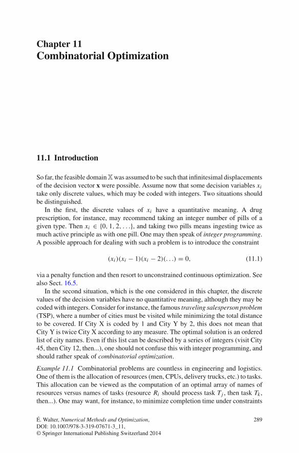
Chapter 11Combinatorial Optimization

11.1 Introduction

So far, the feasible domainXwas assumed to be such that infinitesimal displacementsof the decision vector x were possible. Assume now that some decision variables xi

take only discrete values, which may be coded with integers. Two situations shouldbe distinguished.

In the first, the discrete values of xi have a quantitative meaning. A drugprescription, for instance, may recommend taking an integer number of pills of agiven type. Then xi ∈ {0, 1, 2, . . .}, and taking two pills means ingesting twice asmuch active principle as with one pill. One may then speak of integer programming.A possible approach for dealing with such a problem is to introduce the constraint

(xi )(xi − 1)(xi − 2)(. . .) = 0, (11.1)

via a penalty function and then resort to unconstrained continuous optimization. Seealso Sect. 16.5.

In the second situation, which is the one considered in this chapter, the discretevalues of the decision variables have no quantitative meaning, although they may becoded with integers. Consider for instance, the famous traveling salesperson problem(TSP), where a number of cities must be visited while minimizing the total distanceto be covered. If City X is coded by 1 and City Y by 2, this does not mean thatCity Y is twice City X according to any measure. The optimal solution is an orderedlist of city names. Even if this list can be described by a series of integers (visit City45, then City 12, then...), one should not confuse this with integer programming, andshould rather speak of combinatorial optimization.

Example 11.1 Combinatorial problems are countless in engineering and logistics.One of them is the allocation of resources (men, CPUs, delivery trucks, etc.) to tasks.This allocation can be viewed as the computation of an optimal array of names ofresources versus names of tasks (resource Ri should process task Tj , then task Tk ,then...). One may want, for instance, to minimize completion time under constraints

É. Walter, Numerical Methods and Optimization, 289DOI: 10.1007/978-3-319-07671-3_11,© Springer International Publishing Switzerland 2014

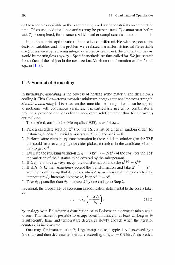
290 11 Combinatorial Optimization

on the resources available or the resources required under constraints on completiontime. Of course, additional constraints may be present (task Ti cannot start beforetask Tj is completed, for instance), which further complicate the matter. �

In combinatorial optimization, the cost is not differentiable with respect to thedecision variables, and if the problem were relaxed to transform it into a differentiableone (for instance by replacing integer variables by real ones), the gradient of the costwould be meaningless anyway... Specific methods are thus called for. We just scratchthe surface of the subject in the next section. Much more information can be found,e.g., in [1–3].

11.2 Simulated Annealing

In metallurgy, annealing is the process of heating some material and then slowlycooling it. This allows atoms to reach a minimum-energy state and improves strength.Simulated annealing [4] is based on the same idea. Although it can also be appliedto problems with continuous variables, it is particularly useful for combinatorialproblems, provided one looks for an acceptable solution rather than for a provablyoptimal one.

The method, attributed to Metropolis (1953), is as follows.

1. Pick a candidate solution x0 (for the TSP, a list of cities in random order, forinstance), choose an initial temperature ∂0 > 0 and set k = 0.

2. Perform some elementary transformation in the candidate solution (for the TSP,this could mean exchanging two cities picked at random in the candidate solutionlist) to get xk+.

3. Evaluate the resulting variation �Jk = J (xk+) − J (xk) of the cost (for the TSP,the variation of the distance to be covered by the salesperson).

4. If �Jk < 0, then always accept the transformation and take xk+1 = xk+5. If �Jk � 0, then sometimes accept the transformation and take xk+1 = xk+,

with a probability δk that decreases when �Jk increases but increases when thetemperature ∂k increases; otherwise, keep xk+1 = xk .

6. Take ∂k+1 smaller than ∂k , increase k by one and go to Step 2.

In general, the probability of accepting a modification detrimental to the cost is takenas

δk = exp

(−�Jk

∂k

), (11.2)

by analogy with Boltzmann’s distribution, with Boltzmann’s constant taken equalto one. This makes it possible to escape local minimizers, at least as long as ∂0is sufficiently large and temperature decreases slowly enough when the iterationcounter k is incremented.

One may, for instance, take ∂0 large compared to a typical �J assessed by afew trials and then decrease temperature according to ∂k+1 = 0.99∂k . A theoretical

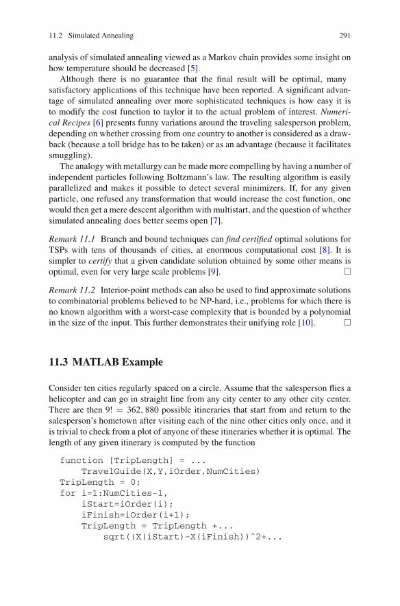
11.2 Simulated Annealing 291

analysis of simulated annealing viewed as a Markov chain provides some insight onhow temperature should be decreased [5].

Although there is no guarantee that the final result will be optimal, manysatisfactory applications of this technique have been reported. A significant advan-tage of simulated annealing over more sophisticated techniques is how easy it isto modify the cost function to taylor it to the actual problem of interest. Numeri-cal Recipes [6] presents funny variations around the traveling salesperson problem,depending on whether crossing from one country to another is considered as a draw-back (because a toll bridge has to be taken) or as an advantage (because it facilitatessmuggling).

The analogy with metallurgy can be made more compelling by having a number ofindependent particles following Boltzmann’s law. The resulting algorithm is easilyparallelized and makes it possible to detect several minimizers. If, for any givenparticle, one refused any transformation that would increase the cost function, onewould then get a mere descent algorithm with multistart, and the question of whethersimulated annealing does better seems open [7].

Remark 11.1 Branch and bound techniques can find certified optimal solutions forTSPs with tens of thousands of cities, at enormous computational cost [8]. It issimpler to certify that a given candidate solution obtained by some other means isoptimal, even for very large scale problems [9]. �

Remark 11.2 Interior-point methods can also be used to find approximate solutionsto combinatorial problems believed to be NP-hard, i.e., problems for which there isno known algorithm with a worst-case complexity that is bounded by a polynomialin the size of the input. This further demonstrates their unifying role [10]. �

11.3 MATLAB Example

Consider ten cities regularly spaced on a circle. Assume that the salesperson flies ahelicopter and can go in straight line from any city center to any other city center.There are then 9! = 362, 880 possible itineraries that start from and return to thesalesperson’s hometown after visiting each of the nine other cities only once, and itis trivial to check from a plot of anyone of these itineraries whether it is optimal. Thelength of any given itinerary is computed by the function

function [TripLength] = ...TravelGuide(X,Y,iOrder,NumCities)

TripLength = 0;for i=1:NumCities-1,

iStart=iOrder(i);iFinish=iOrder(i+1);TripLength = TripLength +...

sqrt((X(iStart)-X(iFinish))ˆ2+...

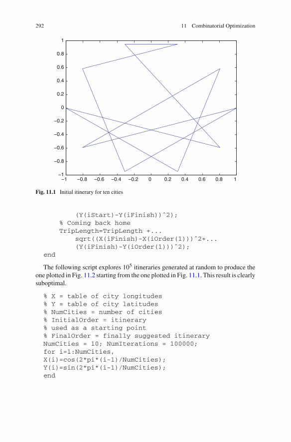
292 11 Combinatorial Optimization

−1 −0.8 −0.6 −0.4 −0.2 0 0.2 0.4 0.6 0.8 1−1

−0.8

−0.6

−0.4

−0.2

0

0.2

0.4

0.6

0.8

1

Fig. 11.1 Initial itinerary for ten cities

(Y(iStart)-Y(iFinish))ˆ2);% Coming back homeTripLength=TripLength +...

sqrt((X(iFinish)-X(iOrder(1)))ˆ2+...(Y(iFinish)-Y(iOrder(1)))ˆ2);

end

The following script explores 105 itineraries generated at random to produce theone plotted in Fig. 11.2 starting from the one plotted in Fig. 11.1. This result is clearlysuboptimal.

% X = table of city longitudes% Y = table of city latitudes% NumCities = number of cities% InitialOrder = itinerary% used as a starting point% FinalOrder = finally suggested itineraryNumCities = 10; NumIterations = 100000;for i=1:NumCities,X(i)=cos(2*pi*(i-1)/NumCities);Y(i)=sin(2*pi*(i-1)/NumCities);end

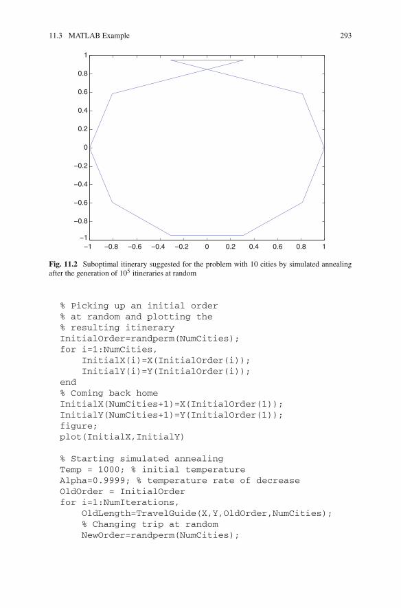
11.3 MATLAB Example 293

−1 −0.8 −0.6 −0.4 −0.2 0 0.2 0.4 0.6 0.8 1−1

−0.8

−0.6

−0.4

−0.2

0

0.2

0.4

0.6

0.8

1

Fig. 11.2 Suboptimal itinerary suggested for the problem with 10 cities by simulated annealingafter the generation of 105 itineraries at random

% Picking up an initial order% at random and plotting the% resulting itineraryInitialOrder=randperm(NumCities);for i=1:NumCities,

InitialX(i)=X(InitialOrder(i));InitialY(i)=Y(InitialOrder(i));

end% Coming back homeInitialX(NumCities+1)=X(InitialOrder(1));InitialY(NumCities+1)=Y(InitialOrder(1));figure;plot(InitialX,InitialY)

% Starting simulated annealingTemp = 1000; % initial temperatureAlpha=0.9999; % temperature rate of decreaseOldOrder = InitialOrderfor i=1:NumIterations,

OldLength=TravelGuide(X,Y,OldOrder,NumCities);% Changing trip at randomNewOrder=randperm(NumCities);

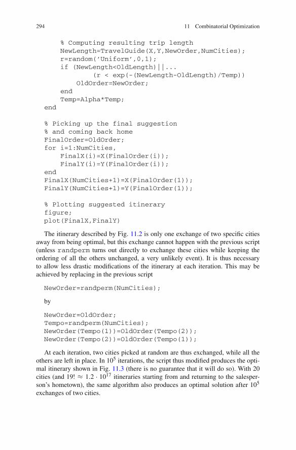
294 11 Combinatorial Optimization

% Computing resulting trip lengthNewLength=TravelGuide(X,Y,NewOrder,NumCities);r=random(’Uniform’,0,1);if (NewLength<OldLength)||...

(r < exp(-(NewLength-OldLength)/Temp))OldOrder=NewOrder;

endTemp=Alpha*Temp;

end

% Picking up the final suggestion% and coming back homeFinalOrder=OldOrder;for i=1:NumCities,

FinalX(i)=X(FinalOrder(i));FinalY(i)=Y(FinalOrder(i));

endFinalX(NumCities+1)=X(FinalOrder(1));FinalY(NumCities+1)=Y(FinalOrder(1));

% Plotting suggested itineraryfigure;plot(FinalX,FinalY)

The itinerary described by Fig. 11.2 is only one exchange of two specific citiesaway from being optimal, but this exchange cannot happen with the previous script(unless randperm turns out directly to exchange these cities while keeping theordering of all the others unchanged, a very unlikely event). It is thus necessaryto allow less drastic modifications of the itinerary at each iteration. This may beachieved by replacing in the previous script

NewOrder=randperm(NumCities);

by

NewOrder=OldOrder;Tempo=randperm(NumCities);NewOrder(Tempo(1))=OldOrder(Tempo(2));NewOrder(Tempo(2))=OldOrder(Tempo(1));

At each iteration, two cities picked at random are thus exchanged, while all theothers are left in place. In 105 iterations, the script thus modified produces the opti-mal itinerary shown in Fig. 11.3 (there is no guarantee that it will do so). With 20cities (and 19! ≈ 1.2 · 1017 itineraries starting from and returning to the salesper-son’s hometown), the same algorithm also produces an optimal solution after 105

exchanges of two cities.

11.3 MATLAB Example 295

−1 −0.8 −0.6 −0.4 −0.2 0 0.2 0.4 0.6 0.8 1−1

−0.8

−0.6

−0.4

−0.2

0

0.2

0.4

0.6

0.8

1

Fig. 11.3 Optimal itinerary suggested for the problem with ten cities by simulated annealing afterthe generation of 105 exchanges of two cities picked at random

It is not clear whether decreasing temperature plays any useful role in thisparticular example. The following script refuses any modification of the itinerarythat would increase the distance to be covered, and yet also produces the optimalitinerary of Fig. 11.5 from the itinerary of Fig. 11.4 for a problem with 20 cities.

NumCities = 20;NumIterations = 100000;for i=1:NumCities,X(i)=cos(2*pi*(i-1)/NumCities);Y(i)=sin(2*pi*(i-1)/NumCities);endInitialOrder=randperm(NumCities);for i=1:NumCities,

InitialX(i)=X(InitialOrder(i));InitialY(i)=Y(InitialOrder(i));

endInitialX(NumCities+1)=X(InitialOrder(1));InitialY(NumCities+1)=Y(InitialOrder(1));

% Plotting initial itineraryfigure;plot(InitialX,InitialY)

296 11 Combinatorial Optimization

−1 −0.8 −0.6 −0.4 −0.2 0 0.2 0.4 0.6 0.8 1−1

−0.8

−0.6

−0.4

−0.2

0

0.2

0.4

0.6

0.8

1

Fig. 11.4 Initial itinerary for 20 cities

−1 −0.8 −0.6 −0.4 −0.2 0 0.2 0.4 0.6 0.8 1

−1

−0.8

−0.6

−0.4

−0.2

0

0.2

0.4

0.6

0.8

1

Fig. 11.5 Optimal itinerary for the problem with 20 cities, obtained after the generation of 105

exchanges of two cities picked at random; no increase in the length of the TSP’s trip has beenaccepted

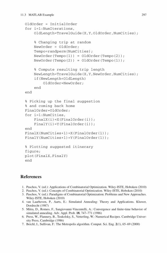
11.3 MATLAB Example 297

OldOrder = InitialOrderfor i=1:NumIterations,

OldLength=TravelGuide(X,Y,OldOrder,NumCities);

% Changing trip at randomNewOrder = OldOrder;Tempo=randperm(NumCities);NewOrder(Tempo(1)) = OldOrder(Tempo(2));NewOrder(Tempo(2)) = OldOrder(Tempo(1));

% Compute resulting trip lengthNewLength=TravelGuide(X,Y,NewOrder,NumCities);if(NewLength<OldLength)

OldOrder=NewOrder;end

end

% Picking up the final suggestion% and coming back homeFinalOrder=OldOrder;for i=1:NumCities,

FinalX(i)=X(FinalOrder(i));FinalY(i)=Y(FinalOrder(i));

endFinalX(NumCities+1)=X(FinalOrder(1));FinalY(NumCities+1)=Y(FinalOrder(1));

% Plotting suggested itineraryfigure;plot(FinalX,FinalY)end

References

1. Paschos, V. (ed.): Applications of Combinatorial Optimization. Wiley-ISTE, Hoboken (2010)2. Paschos, V. (ed.): Concepts of Combinatorial Optimization. Wiley-ISTE, Hoboken (2010)3. Paschos, V. (ed.): Paradigms of Combinatorial Optimization: Problems and New Approaches.

Wiley-ISTE, Hoboken (2010)4. van Laarhoven, P., Aarts, E.: Simulated Annealing: Theory and Applications. Kluwer,

Dordrecht (1987)5. Mitra, D., Romeo, F., Sangiovanni-Vincentelli, A.: Convergence and finite-time behavior of

simulated annealing. Adv. Appl. Prob. 18, 747–771 (1986)6. Press, W., Flannery, B., Teukolsky, S., Vetterling, W.: Numerical Recipes. Cambridge Univer-

sity Press, Cambridge (1986)7. Beichl, I., Sullivan, F.: The Metropolis algorithm. Comput. Sci. Eng. 2(1), 65–69 (2000)

298 11 Combinatorial Optimization

8. Applegate, D., Bixby, R., Chvátal, V., Cook, W.: The Traveling Salesman Problem: A Compu-tational Study. Princeton University Press, Princeton (2006)

9. Applegate, D., Bixby, R., Chvátal, V., Cook, W., Espinoza, D., Goycoolea, M., Helsgaun, K.:Certification of an optimal TSP tour through 85,900 cities. Oper. Res. Lett. 37, 11–15 (2009)

10. Wright, M.: The interior-point revolution in optimization: history, recent developments, andlasting consequences. Bull. Am. Math. Soc. 42(1), 39–56 (2004)

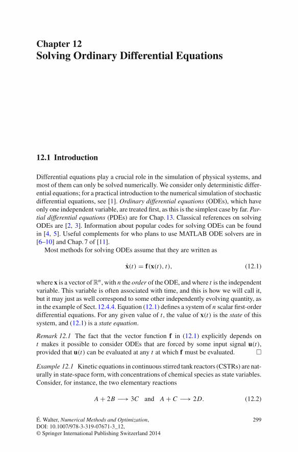
Chapter 12Solving Ordinary Differential Equations

12.1 Introduction

Differential equations play a crucial role in the simulation of physical systems, andmost of them can only be solved numerically. We consider only deterministic differ-ential equations; for a practical introduction to the numerical simulation of stochasticdifferential equations, see [1]. Ordinary differential equations (ODEs), which haveonly one independent variable, are treated first, as this is the simplest case by far. Par-tial differential equations (PDEs) are for Chap. 13. Classical references on solvingODEs are [2, 3]. Information about popular codes for solving ODEs can be foundin [4, 5]. Useful complements for who plans to use MATLAB ODE solvers are in[6–10] and Chap. 7 of [11].

Most methods for solving ODEs assume that they are written as

x(t) = f(x(t), t), (12.1)

where x is a vector ofRn , with n the order of the ODE, and where t is the independentvariable. This variable is often associated with time, and this is how we will call it,but it may just as well correspond to some other independently evolving quantity, asin the example of Sect. 12.4.4. Equation (12.1) defines a system of n scalar first-orderdifferential equations. For any given value of t , the value of x(t) is the state of thissystem, and (12.1) is a state equation.

Remark 12.1 The fact that the vector function f in (12.1) explicitly depends ont makes it possible to consider ODEs that are forced by some input signal u(t),provided that u(t) can be evaluated at any t at which f must be evaluated. �

Example 12.1 Kinetic equations in continuous stirred tank reactors (CSTRs) are nat-urally in state-space form, with concentrations of chemical species as state variables.Consider, for instance, the two elementary reactions

A + 2B −√ 3C and A + C −√ 2D. (12.2)

É. Walter, Numerical Methods and Optimization, 299DOI: 10.1007/978-3-319-07671-3_12,© Springer International Publishing Switzerland 2014

300 12 Solving Ordinary Differential Equations

21u

d0, 1

d1, 2

d2, 1

Fig. 12.1 Example of compartmental model

The corresponding kinetic equations are

[ A] = −k1[A][B]2 − k2[A][C],[B] = −2k1[A][B]2,

[C] = 3k1[A][B]2 − k2[A][C],[D] = 2k2[A][C], (12.3)

where [X ] denotes the concentration of species X . (The rate constants k1 and k2 ofthe two elementary reactions are actually functions of temperature, which may bekept constant or otherwise controlled.) �

Example 12.2 Compartmental models [12], widely used in biology and pharma-cokinetics, consist of tanks (represented by disks) exchanging material as indicatedby arrows (Fig. 12.1). Their state equation is obtained by material balance. The two-compartment model of Fig. 12.1 corresponds to

x1 = −(d0,1 + d2,1) + d1,2 + u,

x2 = d2,1 − d1,2, (12.4)

with u an input flow of material, xi the quantity of material in Compartment i anddi, j the material flow from Compartment j to Compartment i , which is a functionof the state vector x. (The exterior is considered as a special additional compartmentindexed by 0.) If, as often assumed, each material flow is proportional to the quantityof material in the donor compartment:

di, j = ∂i, j x j , (12.5)

then the state equation becomes

x = Ax + Bu, (12.6)

12.1 Introduction 301

which is linear in the input-flow vector u, with A a function of the ∂i, j ’s. For themodel of Fig. 12.1,

A =[−(∂0,1 + ∂2,1) ∂1,2

∂2,1 −∂1,2

⎡(12.7)

and B becomes

b =[

10

⎡, (12.8)

because there is a single scalar input. �

Remark 12.2 Although (12.6) is linear with respect to its input, its solution is stronglynonlinear in A. This has consequences if the unknown parameters ∂i, j are to beestimated from measurements

y(ti ) = Cx(ti ), i = 1, . . . , N , (12.9)

by minimizing some cost function. Even if this cost function is quadratic in the error,the linear least-squares method will not apply because the cost function will not bequadratic in the parameters. �

Remark 12.3 When the vector function f in (12.1) depends not only on x(t) butalso on t , it is possible formally to get rid of the dependency in t by considering theextended state vector

xe(t) =[

xt

⎡. (12.10)

This vector satisfies the extended state equation

xe(t) =[

x(t)1

⎡=

[f(x, t)

1

⎡= fe ⎢

xe(t)⎣, (12.11)

where the vector function fe depends only on the extended state. �

Sometimes, putting ODEs in state-space form requires some work, as in the fol-lowing example, which corresponds to a large class of ODEs.

Example 12.3 Any nth order scalar ODE that can be written as

y(n) = f (y, y, . . . , y(n−1), t) (12.12)

may be put under the form (12.1) by taking

x =

⎤

⎥⎥⎥⎦

yy...

y(n−1)

⎞

⎠⎠⎠ . (12.13)

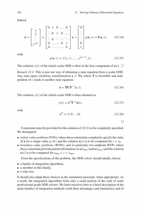
302 12 Solving Ordinary Differential Equations

Indeed,

x =

⎤

⎥⎥⎥⎦

yy...

y(n)

⎞

⎠⎠⎠ =

⎤

⎥⎥⎥⎥⎥⎥⎦

0 1 0 . . . 0... 0 1 0 . . .... 0

. . .. . .

. . .

0 . . . . . . 0 10 . . . . . . . . . 0

⎞

⎠⎠⎠⎠⎠⎠x +

⎤

⎥⎥⎥⎥⎥⎥⎦

0......

01

⎞

⎠⎠⎠⎠⎠⎠g(x, t) = f(x, t), (12.14)

withg(x, t) = f (y, y, . . . , y(n−1), t). (12.15)

The solution y(t) of the initial scalar ODE is then in the first component of x(t). �

Remark 12.4 This is just one way of obtaining a state equation from a scalar ODE.Any state-space similarity transformation z = Tx, where T is invertible and inde-pendent of t , leads to another state equation.

z = Tf(T−1z, t), (12.16)

The solution y(t) of the initial scalar ODE is then obtained as

y(t) = cTT−1z(t), (12.17)

withcT = (1 0 . . . 0). (12.18)

�

Constraints must be provided for the solution of (12.1) to be completely specified.We distinguish

• initial-value problems (IVPs), where these constraints completely specify the valueof x for a single value t0 of t and the solution x(t) is to be computed for t � t0,

• boundary-value problems (BVPs), and in particular two-endpoint BVPs wherethese constraints provide partial information on x(tmin) and x(tmax) and the solutionx(t) is to be computed for tmin � t � tmax.

From the specifications of the problem, the ODE solver should ideally choose

• a family of integration algorithms,• a member in this family,• a step-size.

It should also adapt these choices as the simulation proceeds, when appropriate. Asa result, the integration algorithms form only a small portion of the code of someprofessional-grade ODE solvers. We limit ourselves here to a brief description of themain families of integration methods (with their advantages and limitations) and of

12.1 Introduction 303

how automatic step-size control may be carried out. We start in Sect. 12.2 by IVPs,which are simpler than the BVPs treated in Sect. 12.3.

12.2 Initial-Value Problems

The type of problem considered in this section is the numerical computation, fort � t0, of the solution x(t) of the system

x = f(x, t), (12.19)

with the initial conditionx(t0) = x0, (12.20)

where x0 is numerically known. Equation (12.20) is a Cauchy condition, and this isa Cauchy problem.

Is is assumed that the solution of (12.19) for the initial condition (12.20) exists andis unique. When f(·, ·) is defined on an open set U ∇ R

n ×R, a sufficient conditionfor this assumption to hold true in U is that f be Lipschitz with respect to x, uniformlyrelatively to t . This means that there exists a constant L → R such that

⇒(x, y, t) : (x, t) → U and (y, t) → U, ||f(x, t) − f(y, t)|| � L · ||x − y||. (12.21)

Remark 12.5 Strange phenomena may take place when this Lipschitz condition isnot satisfied, as with the Cauchy problems

x = −px2, x(0) = 1, (12.22)

andx = −x + x2, x(0) = p. (12.23)

It is easy to check that (12.22) admits the solution

x(t) = 1

1 + pt. (12.24)

When p > 0, this solution is valid for any t � 0, but when p < 0, it has a finite escapetime: it tends to infinity when t tends to −1/p and is only valid for t → [0,−1/p).

The nature of the solution of (12.23) depends on the magnitude of p. When |p|is small enough, the effect of the quadratic term is negligible and the solution isapproximately equal to p exp(−t), whereas when |p| is large enough, the quadraticterm dominates and the solution has a finite escape time. �

304 12 Solving Ordinary Differential Equations

Remark 12.6 The final time tf of the computation may not be known in advance,and may be defined as the first time such that

h (x (tf) , tf) = 0, (12.25)

where h (x, t) is some problem-dependent event function. A typical instance iswhen simulating a hybrid system that switches between continuous-time behaviorsdescribed by ODEs, where the ODE changes when the state crosses some boundary.A new Cauchy problem with another ODE and initial time tf has then to be consid-ered. A ball falling on the ground before bouncing up is a very simple example ofsuch a hybrid system, where the ODE to be used once the ball has started hitting theground differs from the one used during free fall. A number of solvers can locateevents and restart integration so as to deal with changes in the ODE [13, 14]. �

12.2.1 Linear Time-Invariant Case

An important special case is when f(x, t) is linear in x and does not depend explicitlyon t , so it can be written as

f(x, t) ∈ Ax(t), (12.26)

where A is a constant, numerically known square matrix. The solution of the Cauchyproblem is then

x(t) = exp[A(t − t0)] · x(t0), (12.27)

where exp[A(t − t0)] is a matrix exponential, which can be computed in manyways [15].

Provided that the norm of M = A(t −t0) is small enough, one may use a truncatedTaylor series expansion

exp M ≈ I + M + 1

2M2 + · · · + 1

q!Mq , (12.28)

or a (p, p) Padé approximation

exp M ≈ [Dp(M)]−1 Np(M), (12.29)

where Np(M) and Dp(M) are pth order polynomials in M. The coefficients of thepolynomials in the Padé approximation are chosen in such a way that its Taylorexpansion is the same as that of exp M up to order q = 2p. Thus

Np(M) =p∑

j=0

c j M j (12.30)

12.2 Initial-Value Problems 305

and

Dp(M) =p∑

j=0

c j (−M) j , (12.31)

with

c j = (2p − j)! p!(2p)! j ! (p − j)! . (12.32)

When A can be diagonalized by a state-space similarity transformation T, suchthat

� = T−1AT, (12.33)

the diagonal entries of � are the eigenvalues λi of A (i = 1, . . . , n), and

exp[A(t − t0)] = T · exp[�(t − t0)] · T−1, (12.34)

where the i th diagonal entry of the diagonal matrix exp[�(t − t0)] is exp[λi (t − t0)].This diagonalization approach makes it easy to evaluate x(ti ) at arbitrary values of ti .

The scaling and squaring method [15–17], based on the relation

exp M =[

exp

(Mm

)⎡m

, (12.35)

is one of the most popular approaches for computing matrix exponentials. It is imple-mented in MATLAB as the function expm. During scaling, m is taken as the smallestpower of two such that ⊂M/m⊂ < 1. A Taylor or Padé approximation is then usedto evaluate exp(M/m), before evaluating exp M by repeated squaring.

Another option is to use one of the general-purpose methods presented next. Seealso Sect. 16.19.

12.2.2 General Case

All of the methods presented in this section involve a positive step-size h on theindependent variable t , assumed constant for the time being. To simplify notation,we write

xl = x(tl) = x(t0 + lh) (12.36)

andfl = f(x(tl), tl). (12.37)

The simplest methods for solving initial-value problems are Euler’s methods.

306 12 Solving Ordinary Differential Equations

12.2.2.1 Euler’s Methods

Starting from xl , the explicit Euler method evaluates xl+1 via a first-order Taylorexpansion of x(t) around t = tl

x(tl + h) = x(tl) + hx(tl) + o(h). (12.38)

It thus takesxl+1 = xl + hfl . (12.39)

It is a single-step method, as the evaluation of x(tl+1) is based on the value of xat a single value tl of t . The method error for one step (or local method error) isgenerically O(h2) (unless x(tl) = 0).

Equation (12.39) boils down to replacing x in (12.1) by the forward finite-difference approximation

x(tl) ≈ xl+1 − xl

h. (12.40)

As the evaluation of xl+1 by (12.39) uses only the past value xl of x, the explicitEuler method is a prediction method.

One may instead replace x in (12.1) by the backward finite-difference approxi-mation

x(tl+1) ≈ xl+1 − xl

h, (12.41)

to getxl+1 = xl + hfl+1. (12.42)

Since fl+1 depends on xl+1, xl+1 is now obtained by solving an implicit equation,and this is the implicit Euler method. It has better stability properties than its explicitcounterpart, as illustrated by the following example.

Example 12.4 Consider the scalar first-order differential equation (n = 1)

x = λx, (12.43)

with λ some negative real constant, so (12.43) is asymptotically stable, i.e., x(t) tendsto zero when t tends to infinity. The explicit Euler method computes

xl+1 = xl + h(λxl) = (1 + λh)xl , (12.44)

which is asymptotically stable if and only if |1 + λh| < 1, i.e., if 0 < −λh < 2.Compare with the implicit Euler method, which computes

xl+1 = xl + h(λxl+1). (12.45)

12.2 Initial-Value Problems 307

The implicit equation (12.45) can be made explicit as

xl+1 = 1

1 − λhxl , (12.46)

which is asymptotically stable for any step-size h since λ < 0 and 0 < 11−λh < 1. �

Except when (12.42) can be made explicit (as in Example 12.4), the implicit Eulermethod is more complicated to implement than the explicit one, and this is true forall the other implicit methods to be presented, see Sect. 12.2.2.4.

12.2.2.2 Runge-Kutta Methods

A natural idea is to build on Euler’s methods by using a higher order Taylor expansionof x(t) around tl

xl+1 = xl + hx(tl) + · · · + hk

k! x(k)(tl) + o(hk). (12.47)

Computation becomes more complicated when k increases, however, since higherorder derivatives of x with respect to t need to be evaluated. This was used as anargument in favor of the much more commonly used Runge-Kutta methods [18]. Theequations of a kth order Runge-Kutta method RK(k) are chosen so as to ensure thatthe coefficients of a Taylor expansion of xl+1 as computed with RK(k) are identicalto those of (12.47) up to order k.

Remark 12.7 The order k of a numerical method for solving ODEs refers to themethod error, and should not be confused with the order n of the ODE. �

The solution of (12.1) between tl and tl+1 = tl + h satisfies

x(tl+1) = x(tl) +tl+1∫

tl

f(x(δ ), δ )dδ. (12.48)

This suggests using numerical quadrature, as in Chap. 6, and writing

xl+1 = xl + hq∑

i=1

bi f(x(tl,i ), tl,i ), (12.49)

where xl is an approximation of x(tl) assumed available, and where

tl,i = tl + δi h, (12.50)

308 12 Solving Ordinary Differential Equations

with 0 � δi � 1. The problem is more difficult than in Chap. 6, however, becausethe value of x(tl,i ) needed in (12.49) is unknown. It is replaced by xl,i , also obtainedby numerical quadrature as

xl,i = xl + hq∑

j=1

ai, j f(xl, j , tl, j ). (12.51)

The q(q + 2) coefficients ai, j , bi and δi of a q-stage Runge-Kutta method must bechosen so as to ensure stability and the highest possible order of accuracy. This leadsto what is called in [19] a nonlinear algebraic jungle, to which civilization and orderwere brought in the pioneering work of J.C. Butcher.

Several sets of Runge-Kutta equations can be obtained for a given order. Theclassical formulas RK(k) are explicit, with ai, j = 0 for i � j , which makes solving(12.51) trivial. For q = 1 and δ1 = 0, one gets RK(1), which is the explicit Eulermethod. One possible choice for RK(2) is

k1 = hf(xl , tl), (12.52)

k2 = hf(xl + k1

2, tl + h

2), (12.53)

xl+1 = xl + k2, (12.54)

tl+1 = tl + h, (12.55)

with a local method error o(h2), generically O(h3). Figure 12.2 illustrates the pro-cedure, assuming a scalar state x .

Although computations are carried out at midpoint tl + h/2, this is a single-stepmethod, as xl+1 is computed as a function of xl .

The most commonly used Runge-Kutta method is RK(4), which may be writtenas

k1 = hf(xl , tl), (12.56)

k2 = hf(xl + k1

2, tl + h

2), (12.57)

k3 = hf(xl + k2

2, tl + h

2), (12.58)

k4 = hf(xl + k3, tl + h), (12.59)

xl+1 = xl + k1

6+ k2

3+ k3

3+ k4

6, (12.60)

tl+1 = tl + h, (12.61)

with a local method error o(h4), generically O(h5). The first derivative of the statewith respect to t is now evaluated once at tl , once at tl+1 and twice at tl +h/2. RK(4)is nevertheless still a single-step method.

12.2 Initial-Value Problems 309

t

x l

t l + h2

t l + 1t l

x l + k 1

2

x l + k1

fl

k1

k2

x l + 1

h

Fig. 12.2 One step of RK(2)

Remark 12.8 Just as the other explicit Runge-Kutta methods, RK(4) is self starting.Provided with the initial condition x0, it computes x1, which is the initial conditionfor computing x2, and so forth. The price to be paid for this nice property is thatnone of the four numerical evaluations of f carried out to compute xl+1 can bereused in the computation of xl+2. This may be a major drawback compared to themultistep methods of Sect. 12.2.2.3, if computational efficiency is important. On theother hand, it is much easier to adapt step-size (see Sect. 12.2.4), and Runge-Kuttamethods are more robust when the solution presents near-discontinuities. They maybe viewed as ocean-going tugboats, which can get large cruise liners out of crowdedharbors and come to their rescue when the sea gets rough. �

Implicit Runge-Kutta methods [19, 20] have also been derived. They are the onlyRunge-Kutta methods that can be used with stiff ODEs, see Sect. 12.2.5. Each of theirsteps requires the solution of an implicit set of equations and is thus more complexfor a given order. Based on [21, 22], MATLAB has implemented its own version ofan implicit Runge-Kutta method in ode23s, where the computation of xl+1 is viathe solution of a system of linear equations [6].

Remark 12.9 It was actually shown in [23], and further discussed in [24], that recur-sion relations often make it possible to use Taylor expansion with less computationthan with a Runge-Kutta method of the same order. The Taylor series approach isindeed used (with quite large values of k) in the context of guaranteed integration,where sets containing the mathematical solutions of the ODEs are computed numer-ically [25–27]. �

310 12 Solving Ordinary Differential Equations

12.2.2.3 Linear Multistep Methods

Linear multistep methods express xl+1 as a linear combination of values of x and x,under the general form

xl+1 =na−1∑

i=0

ai xl−i + hnb+ j0−1∑

j= j0

b j fl− j . (12.62)

They differ by the values given to the number na of ai coefficients, the number nb ofb j coefficients and the initial value j0 of the index in the second sum of (12.62). Assoon as na > 1 or nb > 1 − j0, (12.62) corresponds to a multistep method, becausexl+1 is computed from several past values of x (or of x, which is also computed fromthe value of x).

Remark 12.10 Equation (12.62) only uses evaluations carried out with the constantstep-size h = ti+1 − ti . The evaluations of f used to compute xl+1 can thus be reusedto compute xl+2, which is a considerable advantage over Runge-Kutta methods.There are drawbacks, however:

• adapting step-size gets significantly more complicated than with Runge-Kuttamethods;

• multistep methods are not self-starting; provided with the initial condition x0,they are unable to compute x1, and must receive the help of single-step methodsto compute enough values of x and x to allow the recurrence (12.62) to proceed.

If Runge-Kutta methods are tugboats, then multistep methods are cruise liners, whichcannot leave the harbor of the initial conditions by themselves. Multistep methodsmay also fail later on, if the functions involved are not smooth enough, and Runge-Kutta methods (or other single-step methods) may then have to be called to theirrescue. �

We consider three families of linear multistep methods, namely Adams-Bashforth,Adams-Moulton, and Gear. The kth order member of any of these families has a localmethod error o(hk), generically O(hk+1).

Adams-Bashforth methods are explicit. In the kth order method AB(k), na = 1,a0 = 1, j0 = 0 and nb = k, so

xl+1 = xl + hk−1∑

j=0

b j fl− j . (12.63)

When k = 1, there is a single coefficient b0 = 1 and AB(1) is the explicit Eulermethod

xl+1 = xl + hfl . (12.64)

It is thus a single-step method. AB(2) satisfies

12.2 Initial-Value Problems 311

xl+1 = xl + h

2(3fl − fl−1). (12.65)

It is thus a multistep method, which cannot start by itself, just as AB(3), where

xl+1 = xl + h

12(23fl − 16fl−1 + 5fl−2), (12.66)

and AB(4), where

xl+1 = xl + h

24(55fl − 59fl−1 + 37fl−2 − 9fl−3). (12.67)

In the kth order Adams-Moulton method AM(k), na = 1, a0 = 1, j0 = −1 andnb = k, so

xl+1 = xl + hk−2∑

j=−1

b j fl− j . (12.68)

Since j takes the value −1, all of the Adams-Moulton methods are implicit. Whenk = 1, there is a single coefficient b−1 = 1 and AM(1) is the implicit Euler method

xl+1 = xl + hfl+1. (12.69)

AM(2) is a trapezoidal method (see NC(1) in Sect. 6.2.1.1)

xl+1 = xl + h

2(fl+1 + fl) . (12.70)

AM(3) satisfies

xl+1 = xl + h

12(5fl+1 + 8fl − fl−1) , (12.71)

and is a multistep method, just as AM(4), which is such that

xl+1 = xl + h

24(9fl+1 + 19fl − 5fl−1 + fl−2) . (12.72)

Finally, in the kth order Gear method G(k), na = k, nb = 1 and j0 = −1, so allof the Gear methods are implicit and

xl+1 =k−1∑

i=0

ai xl−i + hbfl+1. (12.73)

The Gear methods are also called BDF methods, because backward-differentiationformulas can be employed to compute their coefficients. G(k) = BDF(k) is such that

312 12 Solving Ordinary Differential Equations

k∑

m=1

1

mαmxl+1 − hfl+1 = 0, (12.74)

with

αxl+1 = xl+1 − xl , (12.75)

α2xl+1 = α(αxl+1) = xl+1 − 2xl + xl−1, (12.76)

and so forth. G(1) is the implicit Euler method

xl+1 = xl + hfl+1. (12.77)

G(2) satisfies

xl+1 = 1

3(4xl − xl−1 + 2hfl+1). (12.78)

G(3) is such that

xl+1 = 1

11(18xl − 9xl−1 + 2xl−2 + 6hfl+1), (12.79)

and G(4) such that

xl+1 = 1

25(48xl − 36xl−1 + 16xl−2 − 3xl−3 + 12hfl+1). (12.80)

A variant of (12.74),

k∑

m=1

1

mαmxl+1 − hfl+1 − ρ

k∑

j=1

1

j(xl+1 − x0

l+1) = 0, (12.81)

was studied in [28] under the name of numerical differentiation formulas (NDF),with the aim of improving on the stability properties of high-order BDF methods.In (12.81), ρ is a scalar parameter and x0

l+1 a (rough) prediction of xl+1 used as aninitial value to solve (12.81) for xl+1 by a simplified Newton (chord) method. Basedon NDFs, MATLAB has implemented its own methodology in ode15s [6, 8], withorder varying from k = 1 to k = 5.

Remark 12.11 Changing the order k of a multistep method when needed is trivial, asit boils down to computing another linear combination of already computed vectorsxl−i or fl−i . This can be taken advantage of to make Adams-Bashforth self-startingby using AB(1) to compute x1 from x0, AB(2) to compute x2 from x1 and x0, andso forth until the desired order has been reached. �

12.2 Initial-Value Problems 313

12.2.2.4 Practical Issues with Implicit Methods

With implicit methods, xl+1 is the solution of a system of equations that can bewritten as

g(xl+1) = 0. (12.82)

This system is nonlinear in general, but becomes linear when (12.26) is satisfied.When possible, as in Example 12.4, it is good practice to put (12.82) in an explicitform where xl+1 is expressed as a function of quantities previously computed. Whenthis cannot be done, one often uses Newton’s method of Sect. 7.4.2 (or a simplifiedversion of it such as the chord method), which requires the numerical or formalevaluation of the Jacobian matrix of g(·). When g(x) is linear in x, its Jacobianmatrix does not depend on x and can be computed once and for all, a considerablesimplification. In MATLAB’s ode15s, Jacobian matrices are evaluated as seldomas possible.

To avoid the repeated and potentially costly numerical solution of (12.82) at eachstep, one may instead alternate

• prediction, where some explicit method (Adams-Bashforth, for instance) is usedto get a first approximation x1

l+1 of xl+1, and• correction, where some implicit method (Adams-Moulton, for instance), is used

to get a second approximation x2l+1 of xl+1, with xl+1 replaced by x1

l+1 whenevaluating fl+1.

The resulting prediction-correction method is explicit, however, so some of the advan-tages of implicit methods are lost.

Example 12.5 Prediction may be carried out with AB(2)

x1l+1 = xl + h

2(3fl − fl−1), (12.83)

and correction with AM(2), where xl+1 on the right-hand side is replaced by x1l+1

x2l+1 = xl + h

2

[f(x1

l+1, tl+1) + fl

], (12.84)

to get an ABM(2) prediction-correction method. �

Remark 12.12 The influence of prediction on the final local method error is lessthan that of correction, so one may use a (k − 1)th order predictor with a kth ordercorrector. When prediction is carried out by AB(1) (i.e., the explicit Euler method)

x1l+1 = xl + hfl , (12.85)

and correction by AM(2) (i.e., the implicit trapezoidal method)

314 12 Solving Ordinary Differential Equations

xl+1 = xl + h

2

[f(x1

l+1, tl+1) + fl

], (12.86)

the result is Heun’s method, a second-order explicit Runge-Kutta method just asRK(2) presented in Sect. 12.2.2.2. �

Adams-Bashforth-Moulton is used in MATLAB’s ode113, from k = 1 tok = 13; advantage is taken of the fact that changing the order of a multistep methodis easy.

12.2.3 Scaling

Provided that upper bounds xi can be obtained on the absolute values of the statevariables xi (i = 1, . . . , n), one may transform the initial state equation (12.1) into

q(t) = g(q(t), t), (12.87)

withqi = xi

xi, i = 1, . . . , n. (12.88)

This was more or less mandatory when analog computers were used, to avoid sat-urating operational amplifiers. The much larger range of magnitudes offered byfloating-point numbers has made this practice less crucial, but it may still turn out tobe very useful.

12.2.4 Choosing Step-Size

When the step-size h is increased, the computational burden decreases, but themethod error increases. Some tradeoff is therefore called for [29]. We consider theinfluence of h on stability before addressing error assessment and step-size tuning.

12.2.4.1 Influence of Step-Size on Stability

Consider a linear time-invariant state equation

x = Ax, (12.89)

and assume that there exists an invertible matrix T such that

A = T�T−1, (12.90)

12.2 Initial-Value Problems 315

where � is a diagonal matrix with the eigenvalues λi (i = 1, . . . , n) of A on itsdiagonal. Assume further that (12.89) is asymptotically stable, so these (possiblycomplex) eigenvalues have strictly negative real parts. Perform the change of coor-dinates q = T−1x to get the new state-space representation

q = T−1ATq = �q. (12.91)

The i th component of the new state vector q satisfies

qi = λi qi . (12.92)

This motivates the study of the stability of numerical methods for solving IVPs onDahlquist’s test problem [30]

x = λx, x(0) = 1, (12.93)

where λ is a complex constant with strictly negative real part rather than the realconstant considered in Example 12.4. The step-size h must be such that the numericalintegration scheme is stable for each of the test equations obtained by replacing λ byone of the eigenvalues of A.

The methodology for conducting this stability study, particularly clearly describedin [31], is now explained; this part may be skipped by the reader interested only inits results.

Single-step methods

When applied to the test problem (12.93), single-step methods compute

xl+1 = R(z)xl , (12.94)

where z = hλ is a complex argument.

Remark 12.13 The exact solution of this test problem satisfies

xl+1 = ehλxl = ez xl , (12.95)

so R(z) is an approximation of ez . Since z is dimensionless, the unit in which t isexpressed has no consequence on the stability results to be obtained, provided thatit is the same for h and λ−1. �

For the explicit Euler method,

xl+1 = xl + hλxl ,

= (1 + z)xl , (12.96)

316 12 Solving Ordinary Differential Equations

so R(z) = 1 + z. For the kth order Taylor method,

xl+1 = xl + hλxl + · · · + 1

k! (hλ)k xl , (12.97)

so R(z) is the polynomial

R(z) = 1 + z + · · · + 1

k! zk . (12.98)

The same holds true for any kth order explicit Runge-Kutta method, as it has beendesigned to achieve this.

Example 12.6 When Heun’s method is applied to the test problem, (12.85) becomes

x1l+1 = xl + hλxl

= (1 + z)xl , (12.99)

and (12.86) translates into

xl+1 = xl + h

2(λx1

l+1 + λxl)

= xl + z

2(1 + z)xl + z

2xl

=(

1 + z + 1

2z2

)xl . (12.100)

This should come as no surprise, as Heun’s method is a second-order explicit Runge-Kutta method. �

For implicit single-step methods, R(z) will be a rational function. For AM(1), theimplicit Euler method,

xl+1 = xl + hλxl+1

= 1

1 − zxl (12.101)

For AM(2), the trapezoidal method,

xl+1 = xl + h

2(λxl+1 + λxl)

= 1 + z2

1 − z2

xl . (12.102)

For each of these methods, the solution of Dahlquist’s test problem will be (absolutely)stable if and only if z is such that |R(z)| � 1 [31].

12.2 Initial-Value Problems 317

Real part of z

Imag

inar

y pa

rt o

f z

−3 −2 −1 0 1−4

−2

0

2

4

Real part of z

Imag

inar

y pa

rt o

f z

−3 −2 −1 0 1−4

−2

0

2

4

Real part of z

Imag

inar

y pa

rt o

f z

−3 −2 −1 0 1−4

−2

0

2

4

Real part of z

Imag

inar

y pa

rt o

f z

−3 −2 −1 0 1−4

−2

0

2

4

Real part of z

Imag

inar

y pa

rt o

f z

−3 −2 −1 0 1−4

−2

0

2

4

Real part of z

Imag

inar

y pa

rt o

f z

−3 −2 −1 0 1−4

−2

0

2

4

Fig. 12.3 Contour plots of the absolute stability regions of explicit Runge-Kutta methods onDahlquist’s test problem, from RK(1) (top left) to RK(6) (bottom right); the region in black isunstable

For the explicit Euler method, this means that hλ should be inside the disk withunit radius centered at −1, whereas for the implicit Euler method, hλ should beoutside the disk with unit radius centered at +1. Since h is always real and positiveand λ is assumed here to have a negative real part, this means that the implicit Eulermethod is always stable on the test problem. The intersection of the stability disk ofthe explicit Euler method with the real axis is the interval [−2, 0], consistent withthe results of Example 12.4.

AM(2) turns out to be absolutely stable for any z with negative real part (i.e., forany λ such that the test problem is stable) and unstable for any other z.

Figure 12.3 presents contour plots of the regions where z = hλ must lie for theexplicit Runge-Kutta methods of order k = 1 to 6 to be absolutely stable. The surface

318 12 Solving Ordinary Differential Equations

of the absolute stability region is found to increase when the order of the method isincreased. See Sect. 12.4.1 for the MATLAB script employed to draw the contourplot for RK(4).

Linear multistep methods

For the test problem (12.93), the vector nonlinear recurrence equation (12.62) thatcontains all linear multistep methods as special cases becomes scalar and linear. Itcan be rewritten as

r∑

j=0

σ j xl+ j = hr∑

j=0

ν jλxl+ j , (12.103)

orr∑

j=0

(σ j − zν j )xl+ j = 0, (12.104)

where r is the number of steps of the method.This linear recurrence equation is absolutely stable if and only if the r roots of its

characteristic polynomial

Pz(β ) =r∑

j=0

(σ j − zν j )βj (12.105)

all belong to the complex disk with unit radius centered on the origin. (More precisely,the simple roots must belong to the closed disk and the multiple roots to the opendisk.)

Example 12.7 Although AB(1), AM(1) and AM(2) are single-step methods, theycan be studied with the characteristic-polynomial approach, with the same results aspreviously. The characteristic polynomial of AB(1) is

Pz(β ) = β − (1 + z), (12.106)

and its single root is βab1 = 1 + z, so the absolute stability region is

S = {z : |1 + z| � 1} . (12.107)

The characteristic polynomial of AM(1) is

Pz(β ) = (1 + z)β − 1, (12.108)

and its single root is βam1 = 1/(1 + z), so the absolute stability region is

12.2 Initial-Value Problems 319

S ={

z :∣∣∣∣

1

1 + z

∣∣∣∣ � 1

}= {z : |1 − z| � 1} . (12.109)

The characteristic polynomial of AM(2) is

Pz(β ) =(

1 − 1

2z

)β −

(1 + 1

2z

), (12.110)

its single root is

βam2 = 1 + 12 z

1 − 12 z

, (12.111)

and |βam2| � 1 ∞ Re(z) � 0. �

When the degree r of the characteristic polynomial is greater than one, the situationbecomes more complicated, as Pz(β ) now has several roots. If z is on the boundaryof the stability region, then at least one root β1 of Pz(β ) must have a modulus equalto one. It thus satisfies

β1 = ei∂ , (12.112)

for some ∂ → [0, 2κ ].Since z acts affinely in (12.105), Pz(β ) can be rewritten as

Pz(β ) = ρ(β ) − z σ(β ). (12.113)

Pz(β1) = 0 then translates into

ρ(ei∂ ) − z σ(ei∂ ) = 0, (12.114)

so

z(∂) = ρ(ei∂ )

σ(ei∂ ). (12.115)

By plotting z(∂) for ∂ → [0, 2κ ], one gets all the values of hλ that may be onthe boundary of the absolute stability region, and this plot is called the boundarylocus. For the explicit Euler method, for instance, ρ(β ) = β − 1 and σ(β ) = 1,so z(∂) = ei∂ − 1 and the boundary locus corresponds to a circle with unit radiuscentered at −1, as it should. When the boundary locus does not cross itself, it separatesthe absolute stability region from the rest of the complex plane and it is a simplematter to decide which is which, by picking up any point z in one of the two regionsand evaluating the roots of Pz(β ) there. When the boundary locus crosses itself, itdefines more than two regions in the complex plane, and each of these regions shouldbe sampled, usually to find that absolute stability is achieved in at most one of them.

In a given family of linear multistep methods, the absolute stability domain tendsto shrink when order is increased, in contrast with what was observed for the explicit

320 12 Solving Ordinary Differential Equations

Runge-Kutta methods. The absolute stability domain of G(6) is so small that it isseldom used, and there is no z such that G(k) is stable for k > 6 [32]. Deteriorationof the absolute stability domain is quicker with Adams-Bashforth methods than withAdams-Moulton methods. For an example of how these regions may be visualized,see the MATLAB script used to draw the absolute stability regions for AB(1) andAB(2) in Sect. 12.4.1.

12.2.4.2 Assessing Local Method Error by Varying Step-Size

When x moves slowly, a larger step-size h may be taken than when it varies quickly,so a constant h may not be appropriate. To avoid useless (or even detrimental) com-putations, a layer is thus added to the code of the ODE solver, in charge of assessinglocal method error in order to adapt h when needed. We start by the simpler case ofsingle-step methods and the older method that proceeds via step-size variation.

Consider RK(4), for instance. Let h1 be the current step-size and xl be the ini-tial state of the current simulation step. Since the local method error of RK(4) isgenerically O(h5), the state after two steps satisfies

x(tl + 2h1) = r1 + h51c1 + h5

1c2 + O(h6), (12.116)

where r1 is the result provided by RK(4), and where

c1 = x(5)(tl)

5! (12.117)

and

c2 = x(5)(tl + h1)

5! . (12.118)

Compute now x(tl + 2h1) starting from the same initial state xl but in a single stepwith size h2 = 2h1, to get

x(tl + h2) = r2 + h52c1 + O(h6), (12.119)

where r2 is the result provided by RK(4).With the approximation c1 = c2 = c (which would be true if the solution were a

polynomial of order at most five), and neglecting all the terms with an order largerthan five, we get

r2 − r1 ≈ (2h51 − h5

2)c = −30h51c. (12.120)

An estimate of the local method error for the step-size h1 is thus

2h51c ≈ r1 − r2

15, (12.121)

12.2 Initial-Value Problems 321

and an estimate of the local method error for h2 is

h52c = (2h1)

5c = 32h51c ≈ 32

30(r1 − r2). (12.122)

As expected, the local method error thus increases considerably when the step-size isdoubled. Since an estimate of this error is now available, one might subtract it fromr1 to improve the quality of the result, but the estimate of the local method errorwould then be lost.

12.2.4.3 Assessing Local Method Error by Varying Order

Instead of varying their step-size to assess their local method error, modern methodstend to vary their order, in such a way that less computation is required. This isthe idea behind embedded Runge-Kutta methods such as the Runge-Kutta-Fehlbergmethods [3]. In RKF45, for instance [33], an RK(5) method is used, such that

x5l+1 = xl +

6∑

i=1

c5,i ki + O(h6). (12.123)

The coefficients of this method are chosen to ensure that an RK(4) method is embed-ded, such that

x4l+1 = xl +

6∑

i=1

c4,i ki + O(h5). (12.124)

The local method error estimate is then taken as ⊂x5l+1 − x4

l+1⊂.MATLAB provides two embedded explicit Runge-Kutta methods, namelyode23,

based on a (2, 3) pair of formulas by Bogacki and Shampine [34] and ode45, basedon a (4, 5) pair of formulas by Dormand and Prince [35]. Dormand and Prince pro-posed a number of other embedded Runge-Kutta methods [35–37], up to a (7, 8) pair.Shampine developed a MATLAB solver based on another Runge-Kutta (7, 8) pairwith strong error control (available from his website), and compared its performancewith that of ode45 in [7].

The local method error of multistep methods can similarly be assessed by com-paring results at different orders. This is easy, as no new evaluation of f is required.

12.2.4.4 Adapting Step-Size

The ODE solver tries to select a step-size that is as large as possible given theprecision requested. It should also take into account the stability constraints of themethod being used (a rule of thumb for nonlinear ODEs is that z = hλ should be inthe absolute-stability region for each eigenvalue λ of the Jacobian matrix of f at thelinearization point).

322 12 Solving Ordinary Differential Equations

If the estimate of local method error on xl+1 turns out to be larger than someuser-specified tolerance, then xl+1 is rejected and knowledge of the method orderis used to assess a reduction in step-size that should make the local method erroracceptable. One should, however, remain realistic in one’s requests for precision, fortwo reasons:

• increasing precision entails reducing step-sizes and thus increasing the computa-tional effort,

• when step-sizes become too small, rounding errors take precedence over methoderrors and the quality of the results degrades.

Remark 12.14 Step-size control based on such crude error estimates as describedin Sects. 12.2.4.2 and 12.2.4.3 may be unreliable. An example is given in [38] forwhich a production-grade code increased the actual error when the error tolerancewas decreased. A class of very simple problems for which the MATLAB solverode45 with default options gives fundamentally incorrect results because its step-size often lies outside the stability region is presented in [39]. �

While changing step-size with a single-step method is easy, it becomes much morecomplicated with a multistep method, as several past values of x must be updatedwhen h is modified. Let Z(h) be the matrix obtained by placing side by side all thepast values of the state vector on which the computation of xl+1 is based

Z(h) = [xl , xl−1, . . . , xl−k]. (12.125)

To replace the step-size hold by hnew, one needs in principle to replace Z(hold) byZ(hnew), which seems to require the knowledge of unknown past values of the state.

Finite-difference approximations such as

x(tl) ≈ xl − xl−1

h(12.126)

and

x(tl) ≈ xl − 2xl−1 + xl−2

h2 (12.127)

make it possible to evaluate numerically

X = [x(tl), x(tl), . . . , x(k)(tl)], (12.128)

and to define a bijective linear transformation T(h) such that

X ≈ Z(h)T(h). (12.129)

For k = 2, and (12.126) and (12.127), one gets, for instance,

12.2 Initial-Value Problems 323

T(h) =

⎤

⎥⎥⎥⎦

1 1h

1h2

0 − 1h − 2

h2

0 0 1h2

⎞

⎠⎠⎠ . (12.130)

Since the mathematical value of X does not depend on h, we have

Z(hnew) ≈ Z(hold)T(hold)T−1(hnew), (12.131)

which allows step-size adaptation without the need for a new start-up via a single-stepmethod.

SinceT(h) = ND(h), (12.132)

with N a constant, invertible matrix and

D(h) = diag(1,1

h,

1

h2 , . . . ), (12.133)

the computation of Z(hnew) by (12.131) can be simplified into that of

Z(hnew) ≈ Z(hold) · N · diag(1, σ, σ2, . . . , σk) · N−1, (12.134)

where σ = hnew/hold. Further simplification is made possible by using the Nordsieckvector, which contains the coefficients of the Taylor expansion of x around tl up toorder k

n(tl , h) =[

x(tl), hx(tl), . . . ,hk

k! x (k)(tl)

⎡T

, (12.135)

with x any given component of x. It can be shown that

n(tl , h) ≈ Mv(tl , h), (12.136)

where M is a known, constant, invertible matrix and

v(tl , h) = [x(tl), x(tl − h), . . . , x(tl − kh)]T. (12.137)

Sincen(tl , hnew) = diag(1, σ, σ2, . . . , σk) · n(tl , hold), (12.138)

it is easy to get an approximate value of v(tl , hnew) as M−1n(tl , hnew), with the orderof approximation unchanged.

324 12 Solving Ordinary Differential Equations

12.2.4.5 Assessing Global Method Error

What is evaluated in Sects. 12.2.4.2 and 12.2.4.3 is the local method error on onestep, and not the global method error at the end of a simulation that may involvemany such steps. The total number of steps is approximately

N = tf − t0h

, (12.139)

with h the average step-size. If the global error of a method with order k was equalto N times its local error, it would be NO(hk+1) = O(hk). The situation is actuallymore complicated, as the global method error crucially depends on how stable theODE is. Let s(tN , x0, t0) be the true value of a solution x(tN ) at the end of a simulationstarted from x0 at t0 and let xN be the estimate of this solution as provided by theintegration method. For any v → R

n , the norm of the global error satisfies

⊂s(tN , x0, t0) − xN ⊂ = ⊂s(tN , x0, t0) − xN + v − v⊂� ⊂v − xN ⊂ + ⊂s(tN , x0, t0) − v⊂. (12.140)

Take v = s(tN , xN−1, tN−1). The first term on the right-hand side of (12.140) is thenthe norm of the last local error, while the second one is the norm of the differencebetween exact solutions evaluated at the same time but starting from different initialconditions. When the ODE is unstable, unavoidable errors in the initial conditions getamplified until the numerical solution becomes useless. On the other hand, when theODE is so stable that the effect of errors in its initial conditions disappears quickly,the global error may be much less than could have been feared.

A simple, rough way to assess the global method error for a given IVP is to solveit a second time with a reduced tolerance and to estimate the error on the first seriesof results by comparing them with those of the second series [29]. One should atleast check that the results of an entire simulation do not vary drastically when theuser-specified tolerance is reduced. While this might help one detect unacceptableerrors, it cannot prove that the results are correct, however.

One might wish instead to characterize global error by providing numerical inter-val vectors [xmin(t), xmax(t)] to which the mathematical solution x(t) belongs atany given t of interest, with all the sources of errors taken into account (includingrounding errors). This is achieved in the context of guaranteed integration [25–27].The challenge is in containing the growth of the uncertainty intervals, which maybecome uselessly pessimistic when t increases.

12.2.4.6 Bulirsch-Stoer Method

The Bulirsch-Stoer method [3] is yet another application of Richardson’s extrapo-lation. A modified midpoint integration method is used to compute x(tl + H) fromx(tl) by a series of N substeps of size h, as follows:

12.2 Initial-Value Problems 325

z0 = x(tl),

z1 = z0 + hf(z0, tl),

zi+1 = zi−1 + 2hf(zi , tl + ih), i = 1, . . . , N − 1,

x(tl + H) = x(tl + Nh) ≈ 1

2[zN + zN−1 + hf(zN , tl + Nh)].

A crucial advantage of this choice is that the method-error term in the computationof x(tl + H) is strictly even (it is a function of h2 rather than of h). The order ofthe method error is thus increased by two with each Richardson extrapolation step,just as with Romberg integration (see Sect. 6.2.2). Extremely accurate results are thusobtained quickly, provided that the solution of the ODE is smooth enough. This makesthe Bulirsch-Stoer method particularly appropriate when a high precision is requiredor when the evaluation of f(x, t) is expensive. Although rational extrapolation wasinitially used, polynomial extrapolation now tends to be favored.

12.2.5 Stiff ODEs

Consider the linear time-invariant state-space model

x = Ax, (12.141)

and assume it is asymptotically stable, i.e., all its eigenvalues have strictly negativereal parts. This model is stiff if the absolute values of these real parts are such thatthe ratio of the largest to the smallest is very large. Similarly, the nonlinear model

x = f(x) (12.142)

is stiff if its dynamics comprises very slow and very fast components. This oftenhappens in chemical reactions, for instance, where rate constants may differ byseveral orders of magnitude.

Stiff ODEs are particularly difficult to solve accurately, as the fast componentsrequire a small step-size, whereas the slow components require a long horizon ofintegration. Even when the fast components become negligible in the solution andone could dream of increasing step-size, explicit integration methods will continueto demand a small step-size to ensure stability. As a result, solving a stiff ODE with amethod for non-stiff problems, such as MATLAB’s ode23 or ode45 may be muchtoo slow to be practical. Implicit methods, including implicit Runge-Kutta methodssuch as ode23s and Gear methods and their variants such as ode15s, may thensave the day [40]. Prediction-correction methods such as ode113 do not qualify asimplicit and should be avoided in the context of stiff ODEs.

326 12 Solving Ordinary Differential Equations

12.2.6 Differential Algebraic Equations

Differential algebraic equations (or DAEs) can be written as

r(q(t), q(t), t) = 0. (12.143)

An important special case is when they can be expressed as an ODE in state-spaceform coupled with algebraic constraints

x = f(x, z, t), (12.144)

0 = g(x, z, t). (12.145)

Singular perturbations are a great provider of such systems.

12.2.6.1 Singular Perturbations

Assume that the state of a system can be split into a slow part x and a fast part z,such that

x = f(x, z, t, ε), (12.146)

x(t0) = x0(ε), (12.147)

εz = g(x, z, t, ε), (12.148)

z(t0) = z0(ε), (12.149)

with ε a positive parameter treated as a small perturbation term. The smaller ε is,the stiffer the system of ODEs becomes. In the limit, when ε is taken equal to zero,(12.148) becomes an algebraic equation

g(x, z, t, 0) = 0, (12.150)

and a DAE is obtained. The perturbation is called singular because the dimension ofthe state space changes when ε becomes equal to zero.

It is sometimes possible, as in the next example, to solve (12.150) for z explicitlyas a function of x and t , and to plug the resulting formal expression in (12.146) to geta reduced-order ODE in state-space form, with the initial condition x(t0) = x0(0).

Example 12.8 Enzyme-substrate reactionConsider the biochemical reaction

E + S � C √ E + P, (12.151)

where E , S, C and P are the enzyme, substrate, enzyme-substrate complex andproduct, respectively. This reaction is usually assumed to follow the equations

12.2 Initial-Value Problems 327

[E] = −k1[E][S] + k−1[C] + k2[C], (12.152)

[S] = −k1[E][S] + k−1[C], (12.153)

[C] = k1[E][S] − k−1[C] − k2[C], (12.154)

[P] = k2[C], (12.155)

with the initial conditions

[E](t0) = E0, (12.156)

[S](t0) = S0, (12.157)

[C](t0) = 0, (12.158)

[P](t0) = 0. (12.159)

Sum (12.152) and (12.154) to prove that [E] + [C] ∈ 0, and eliminate (12.152) bysubstituting E0 − [C] for [E] in (12.153) and (12.154) to get the reduced model

[S] = −k1(E0 − [C])[S] + k−1[C], (12.160)

[C] = k1(E0 − [C])[S] − (k−1 + k2)[C], (12.161)

[S](t0) = S0, (12.162)

[C](t0) = 0. (12.163)

The quasi-steady-state approach [41] then assumes that, after some short transientand before [S] is depleted, the rate with which P is produced is approximatelyconstant. Equation (12.155) then implies that [C] is approximately constant too,which transforms the ODE into a DAE

[S] = −k1(E0 − [C])[S] + k−1[C], (12.164)

0 = k1(E0 − [C])[S] − (k−1 + k2)[C]. (12.165)

The situation is simple enough here to make it possible to get a closed-form expressionof [C] as a function of [S] and the kinetic constants

p = (k1, k−1, k2)T, (12.166)

namely

[C] = E0[S]Km + [S] , (12.167)

with

Km = k−1 + k2

k1. (12.168)

[C] can then be replaced in (12.164) by its closed-form expression (12.167) to getan ODE where [S] is expressed as a function of [S], E0 and p. �

328 12 Solving Ordinary Differential Equations

Extensions of the quasi-steady-state approach to more general models are pre-sented in [42, 43]. When an explicit solution of the algebraic equation is not avail-able, repeated differentiation may be used to transform a DAE into an ODE, seeSect. 12.2.6.2. Another option is to try a finite-difference approach, see Sect. 12.3.3.

12.2.6.2 Repeated Differentiation

By formally differentiating (12.145) with respect to t as many times as needed andreplacing any xi thus created by its expression taken from (12.144), one can obtainan ODE, as illustrated by the following example:

Example 12.9 Consider again Example 12.8 and the DAE (12.164, 12.165), butassume now that no closed-form solution of (12.165) for [C] is available. Differentiate(12.165) with respect to t , to get

k1(E0 − [C])[S] − k1[S][C] − (k−1 + k2)[C] = 0, (12.169)

and thus

[C] = k1(E0 − [C])k−1 + k2 + k1[S] [S], (12.170)

where [S] is given by (12.164) and the denominator cannot vanish. The DAE hasthus been transformed into the ODE

[S] = −k1(E0 − [C])[S] + k−1[C], (12.171)

[C] = k1(E0 − [C])k−1 + k2 + k1[S] {−k1(E0 − [C])[S] + k−1[C]}, (12.172)

and the initial conditions should be chosen so as to satisfy (12.165). �

The differential index of a DAE is the number of differentiations needed to trans-form it into an ODE. In Example 12.9, this index is equal to one.

A useful reminder of difficulties that may be encountered when solving a DAEwith tools intended for ODEs is [44].

12.3 Boundary-Value Problems

What is known about the initial conditions does not always specify them uniquely.Additional boundary conditions must then be provided. When some of the boundaryconditions are not relative to the initial state, a boundary-value problem (or BVP)is obtained. In the present context of ODEs, an important special case is the two-endpoint BVP, where the initial and terminal states are partly specified. BVPs turnout to be more complicated to solve than IVPs.

12.3 Boundary-Value Problems 329

y

xx target

θ

O cannon

Fig. 12.4 A 2D battlefield

Remark 12.15 Many methods for solving BVPs for ODEs also apply mutatis mutan-dis to PDEs, so this part may serve as an introduction to the next chapter. �

12.3.1 A Tiny Battlefield Example

Consider the two-dimensional battlefield illustrated in Fig. 12.4.The cannon at the origin O (x = y = 0) must shoot a motionless target located

at (x = xtarget, y = 0). The modulus v0 of the shell initial velocity is fixed, and thegunner can only choose the aiming angle ∂ in the open interval

⎢0, κ

2

⎣. When drag

is neglected, the shell altitude before impact satisfies

yshell(t) = (v0 sin ∂)(t − t0) − g

2(t − t0)

2, (12.173)

with g the acceleration due to gravity and t0 the instant of time at which the cannonwas fired. The horizontal distance covered by the shell before impact is such that

xshell(t) = (v0 cos ∂)(t − t0). (12.174)

The gunner must thus find ∂ such that there exists t > t0 at which xshell(t) = xtargetand yshell(t) = 0, or equivalently

330 12 Solving Ordinary Differential Equations

(v0 cos ∂)(t − t0) = xtarget, (12.175)

and(v0 sin ∂)(t − t0) = g

2(t − t0)

2. (12.176)

This is a two-endpoint BVP, as we have partial information on the initial and finalstates of the shell. For any feasible numerical value of ∂ , computing the shell trajectoryis an IVP with a unique solution, but this does not imply that the solution of the BVPis unique or even exists.

This example is so simple that the number of solutions is easy to find analytically.Solve (12.176) for (t − t0) and plug the result in (12.175) to get

xtarget = 2 sin(∂) cos(∂)v2

0

g= sin(2∂)

v20

g. (12.177)

For ∂ to exist, xtarget must thus not exceed the maximal range v20/g of the gun. For any

attainable xtarget, there are generically two values ∂1 and ∂2 of ∂ for which (12.177)is satisfied, as any pétanque player knows. These values are symmetric with respectto ∂ = κ/4, and the maximal range is reached when ∂1 = ∂2 = κ/4. Depending onthe conditions imposed on the final state, the number of solutions of this BVP maythus be zero, one, or two.

Not knowing a priori whether a solution exists is a typical difficulty with BVPs.We assume in what follows that the BVP has at least one solution.

12.3.2 Shooting Methods

In shooting methods, thus called by analogy with artillery and the example ofSect. 12.3.1, a vector x0(p) satisfying what is known about the initial conditionsis used, with p a vector of parameters embodying the remaining degrees of freedomin the initial conditions. For any given numerical value of p, x0(p) is numericallyknown so computing the state trajectory becomes an IVP, for which the methods ofSect. 12.2 can be used. The vector p must then be tuned so as to satisfy the otherboundary conditions. One may, for instance, minimize

J (p) = ⊂σ − σ(x0(p))⊂22, (12.178)

where σ is a vector of desired boundary conditions (for instance, terminal conditions),and σ(x0(p)) is a vector of achieved boundary conditions. See Chap. 9 for methodsthat may be used in this context.

12.3 Boundary-Value Problems 331

Alternatively, one may solveσ(x0(p)) = σ, (12.179)

for p, see Chaps. 3 and 7 for methods for doing so.

Remark 12.16 Minimizing (12.178) or solving (12.179) may involve solving a num-ber of IVPs if the state equation is nonlinear. �

Remark 12.17 Shooting methods are a viable option only when the ODEs are stableenough for their numerical solution not to blow up before the end of the integrationinterval required for the solution of the associated IVPs. �

12.3.3 Finite-Difference Method

We assume here that the ODE is written as

g(t, y, y, . . . , y(n)) = 0, (12.180)

and that it is not possible (or not desirable) to put it in state-space form. The principleof the finite-difference method (FDM) is then as follows:

• Discretize the interval of interest for the independent variable t , using regularlyspaced points tl . If the approximate solution is to be computed at tl , l = 1, . . . , N ,make sure that the grid also contains any additional points needed to take intoaccount the information provided by the boundary conditions.

• Substitute finite-difference approximations for the derivatives y( j) in (12.180), forinstance using the centered-difference approximations

yl ≈ Yl+1 − Yl−1

2h(12.181)

and

yl ≈ Yl+1 − 2Yl + Yl−1

h2 , (12.182)

where Yl denotes the approximate solution of (12.180) at the discretization pointindexed by l and

h = tl − tl−1. (12.183)

• Write down the resulting equations at l = 1, . . . , N , taking into account theinformation provided by the boundary conditions where needed, to get a systemof N scalar equations in N unknowns Yl .

• Solve this system, which will be linear if the ODE is linear (see Chap. 3). Whenthe ODE is nonlinear, solution will most often be iterative (see Chap. 7) and basedon linearization, so solving systems of linear equations plays a key role in both

332 12 Solving Ordinary Differential Equations

cases. Because the finite-difference approximations are local (they involve only afew grid points close to those at which the derivative is approximated), the linearsystems to be solved are sparse, and often diagonally dominant.

Example 12.10 Assume that the time-varying linear ODE

y(t) + a1(t)y(t) + a2(t)y(t) = u(t) (12.184)

must satisfy the boundary conditions y(t0) = y0 and y (tf) = yf, with t0, tf, y0 and yfknown (such conditions on the value of the solution at the boundary of the domainare called Dirichlet conditions). Assume also that the coefficients a1(t), a2(t) andthe input u(t) are known for any t in [t0, tf].

Rather than using a shooting method to find the appropriate value for y(t0), takethe grid

tl = t0 + lh, l = 0, . . . , N + 1, with h = tf − t0N + 1

, (12.185)

which has N interior points (not counting the boundary points t0 and tf). Denote byYl the approximate value of y(tl) to be computed (l = 1, . . . , N ), with Y0 = y0 andYN+1 = yf. Plug (12.181) and (12.182) into (12.184) to get

Yl+1 − 2Yl + Yl−1

h2 + a1(tl)Yl+1 − Yl−1

2h+ a2(tl)Y (tl) = u(tl). (12.186)

Rearrange (12.186) as

alYl−1 + blYl + clYl+1 = h2ul , (12.187)

with

al = 1 − h

2a1(tl),

bl = h2a2(tl) − 2,

cl = 1 + h

2a1(tl),

ul = u(tl). (12.188)

Write (12.187) at l = 1, 2, . . . , N , to get

Ax = b, (12.189)

with

12.3 Boundary-Value Problems 333

A =

⎤

⎥⎥⎥⎥⎥⎥⎥⎥⎥⎥⎦

b1 c1 0 . . . . . . 0

a2 b2 c2 0...

0 a3. . .

. . .. . .

...... 0

. . .. . .

. . . 0...

. . . aN−1 bN−1 cN−10 . . . . . . 0 aN bN

⎞

⎠⎠⎠⎠⎠⎠⎠⎠⎠⎠

, (12.190)

x =

⎤

⎥⎥⎥⎥⎥⎦

Y1Y2...

YN−1YN

⎞

⎠⎠⎠⎠⎠and b =

⎤

⎥⎥⎥⎥⎥⎦

h2u1 − a1 y0

h2u2...

h2uN−1

h2uN − cN yf

⎞

⎠⎠⎠⎠⎠. (12.191)

Since A is tridiagonal, solving (12.189) for x has very low complexity and can beachieved quickly, even for large N . Moreover, the method can be used for unstableODEs, contrary to shooting. �

Remark 12.18 The finite-difference approach may also be used to solve IVPs orDAEs. �

12.3.4 Projection Methods

Projection methods for BVPs include the collocation, Ritz-Galerkin and least-squaresapproaches [45]. Splines play a prominent role in these methods [46]. Let α be apartition of the interval I = [t0, tf] into n subintervals [ti−1, ti ], i = 1, . . . , n, suchthat

t0 < t1 < · · · < tn = tf. (12.192)

Splines are elements of the set S(r, k,α) of all piecewise polynomial functions thatare k times continuously differentiable on [t0, tf] and take the same value as somepolynomial of degree at most r on [ti−1, ti ], i = 1, . . . , n. The dimension N ofS(r, k,α) is equal to the number of scalar parameters (and thus to the number ofequations) needed to specify a given spline function in S(r, k,α). The cubic splinesof Sect. 5.3.2 belong to S(3, 2,α), but many other choices are possible. Bernsteinpolynomials, at the core of the computer-aided design of shapes [47], are an attractivealternative considered in [48].

Example 12.10 will be used to illustrate the collocation, Ritz-Galerkin and least-squares approaches as simply as possible.

334 12 Solving Ordinary Differential Equations

12.3.4.1 Collocation

For Example 12.10, collocation methods determine an approximate solution yN →S(r, k,α) such that the N following equations are satisfied:

yN (xi ) + a1(xi )yN (xi ) + a2(xi )yN (xi ) = u(xi ), i = 1, . . . , N − 2, (12.193)

yN (t0) = y0 and yN (tf) = yf. (12.194)

The xi ’s at which yN must satisfy the ODE are the collocation points. Evaluatingthe derivatives of yN that appear in (12.193) is easy, as yN (·) is polynomial in anygiven subinterval. For S(3, 2,α), there is no need to introduce additional equationsbecause of the differentiability constraints, so xi = ti and N = n + 1.

More information on the collocation approach to solving BVPs, including theconsideration of nonlinear problems, is in [49]. Information on the MATLAB solverbvp4c can be found in [9, 50].

12.3.4.2 Ritz-Galerkin Methods

The fascinating history of the Ritz-Galerkin family of methods is recounted in [51].The approach was developed by Ritz in a theoretical setting, and applied by Galerkin(who did attribute it to Ritz) on a number of engineering problems. Figures in Euler’swork suggest that he used the idea without even bothering about explaining it.

Consider the ODELt (y) = u(t), (12.195)

where L(·) is a linear differential operator, Lt (y) is the value taken by L(y) at t , andu is a known input function. Assume that the boundary conditions are

y(t j ) = y j , j = 1, . . . , m, (12.196)

with the y j ’s known. To take (12.196) into account, approximate y(t) by a linearcombination yN (t) of known basis functions (for instance splines)

yN (t) =N∑

j=1

x jφ j (t) + φ0(t), (12.197)

with φ0(·) such thatφ0(ti ) = yi , i = 1, . . . , m, (12.198)

and the other basis functions φ j (·), j = 1, . . . , N , such that

φ j (ti ) = 0, i = 1, . . . , m. (12.199)

12.3 Boundary-Value Problems 335

The approximate solution is thus

yN (t) = �T(t)x + φ0(t), (12.200)

with�(t) = [φ1(t), . . . , φN (t)]T (12.201)

a vector of known basis functions, and

x = (x1, . . . , xN )T (12.202)

a vector of constant coefficients to be determined. As a result, the approximatesolution yN lives in a finite-dimensional space.

Ritz-Galerkin methods then look for x such that

< L(yN − φ0), ϕi >=< u − L(φ0), ϕi >, i = 1, . . . , N , (12.203)

where < ·, · > is the inner product in the function space and the ϕi ’s are known testfunctions. We choose basis and test functions that are square integrable on I, and take

< f1, f2 >=∫

I

f1(δ ) f2(δ )dδ. (12.204)

Since< L(yn − φ0), ϕi >=< L(�Tx), ϕi >, (12.205)

which is linear in x, (12.203) translates into a system of linear equations

Ax = b. (12.206)

The Ritz-Galerkin methods usually take identical basis and test functions, such that

φi → S(r, k,α), ϕi = φi , i = 1, . . . , N , (12.207)

but there is no obligation to do so. Collocation corresponds to taking ϕi (t) = δ(t−ti ),where δ(t − ti ) is the Dirac measure with a unit mass at t = ti , as

< f, ϕi >=∫

I

f (δ )δ(δ − ti )dδ = f (ti ) (12.208)

for any ti in I.

Example 12.11 Consider again Example 12.10, where

Lt (y) = y(t) + a1(t)y(t) + a2(t)y(t). (12.209)

336 12 Solving Ordinary Differential Equations

Take φ0(·) such thatφ0(t0) = y0 and φ0 (tf) = yf. (12.210)

For instanceφ0(t) = yf − y0

tf − t0(t − t0) + y0. (12.211)

Equation (12.206) is satisfied, with

ai, j =∫

I

[φ j (δ ) + a1(δ )φ j (δ ) + a2(δ )φ j (δ )]φi (δ )dδ (12.212)

and

bi =∫

I

[u(δ ) − φ0(δ ) − a1(δ )φ0(δ ) − a2(δ )φ0(δ )]φi (δ )dδ, (12.213)

for i = 1, . . . , N and j = 1, . . . , N .

Integration by parts may be used to decrease the number of derivations needed in(12.212) and (12.213). Since (12.199) translates into

φi (t0) = φi (tf) = 0, i = 1, . . . , N , (12.214)

we have∫

I

φ j (δ )φi (δ )dδ = −∫

I

φ j (δ )φi (δ )dδ, (12.215)

−∫

I

φ0(δ )φi (δ )dδ =∫

I

φ0(δ )φi (δ )dδ. (12.216)

�

The definite integrals involved are often evaluated by Gaussian quadrature on eachof the subintervals generated by α. If the total number of quadrature points wereequal to the dimension of x, Ritz-Galerkin would amount to collocation at thesequadrature points, but more quadrature points are used in general [45].

The Ritz-Galerkin methodology can be extended to nonlinear problems.

12.3.4.3 Least Squares

While the approximate solution obtained by the Ritz-Galerkin approach satisfies theboundary conditions by construction, it does not, in general, satisfy the differentialequation (12.195), so the function

12.3 Boundary-Value Problems 337

ex(t) = Lt (yN ) − u(t) = Lt (�Tx) + Lt (φ0) − u(t) (12.217)

will not be identically zero on I. One may thus attempt to minimize

J (x) =∫

I

e2x(δ )dδ. (12.218)

Since ex(δ ) is affine in x, J (x) is quadratic in x and the continuous-time versionof linear least-squares can be employed. The optimal value x of x thus satisfies thenormal equation

Ax = b, (12.219)

with

A =∫

I

[Lδ (�)][Lδ (�)]Tdδ (12.220)

and

b =∫

I

[Lδ (�)][u(δ ) − Lδ (φ0)]dδ. (12.221)

See [52] for more details (including a more general type of boundary conditionand the treatment of systems of ODEs) and a comparison with the results obtainedwith the Ritz-Galerkin method on numerical examples. A comparison of the threeprojection approaches of Sect. 12.3.4 can be found in [53, 54].

12.4 MATLAB Examples

12.4.1 Absolute Stability Regions for Dahlquist’s Test

Brute-force gridding is used for characterizing the absolute stability region of RK(4)before exploiting characteristic equations to plot the boundaries of the absolute sta-bility regions of AB(1) and AB(2).

12.4.1.1 RK(4)

We take advantage of (12.98), which implies for RK(4) that

R(z) = 1 + z + 1

2z2 + 1

6z3 + 1

24z4. (12.222)

338 12 Solving Ordinary Differential Equations

The region of absolute stability is the set of all z’s such that |R(z)| � 1. The script

clear all[X,Y] = meshgrid(-3:0.05:1,-3:0.05:3);Z = X + i*Y;modR=abs(1+Z+Z.ˆ2/2+Z.ˆ3/6+Z.ˆ4/24);GoodR = ((1-modR)+abs(1-modR))/2;

% 3D surface plotfigure;surf(X,Y,GoodR);colormap(gray)xlabel(’Real part of z’)ylabel(’Imaginary part of z’)zlabel(’Margin of stability’)

% Filled 2D contour plotfigure;contourf(X,Y,GoodR,15);colormap(gray)xlabel(’Real part of z’)ylabel(’Imaginary part of z’)

yields Figs. 12.5 and 12.6.

12.4.1.2 AB(1) and AB(2)

Any point on the boundary of the region of absolute stability of AB(1) must be suchthat the modulus of the root of (12.106) is equal to one. This implies that there existssome ∂ such that exp(i∂) = 1 + z, so

z = exp(i∂) − 1. (12.223)

AB(2) satisfies the recurrence equation (12.65), the characteristic polynomial ofwhich is

Pz(β ) = β 2 −(

1 + 3

2z

)β + z

2. (12.224)

For β = exp(i∂) to be a root of this characteristic equation, z must be such that

exp(2i∂) −(

1 + 3

2z

)exp(i∂) + z

2= 0, (12.225)

which implies that

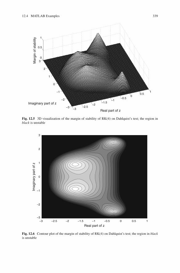
12.4 MATLAB Examples 339

−3−2.5

−2−1.5

−1−0.5

00.5

1

−3

−2

−1

0

1

2

30

0.5

1

Real part of z

Imaginary part of z

Mar

gin

of s

tabi

lity

Fig. 12.5 3D visualization of the margin of stability of RK(4) on Dahlquist’s test; the region inblack is unstable

Real part of z

Imag

inar

y pa

rt o

f z

−3 −2.5 −2 −1.5 −1 −0.5 0 0.5 1−3

−2

−1

0

1

2

3

Fig. 12.6 Contour plot of the margin of stability of RK(4) on Dahlquist’s test; the region in blackis unstable

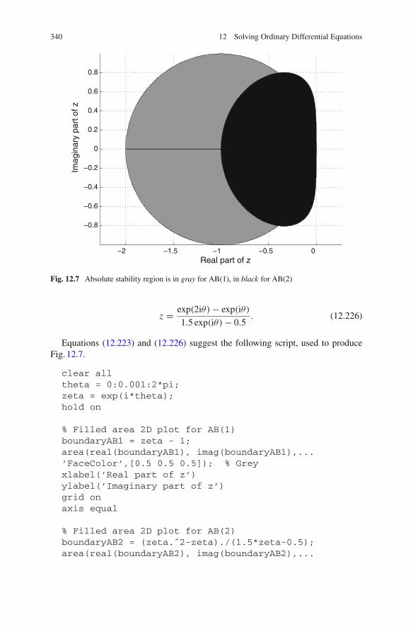
340 12 Solving Ordinary Differential Equations

−2 −1.5 −1 −0.5 0

−0.8

−0.6

−0.4

−0.2

0

0.2

0.4

0.6

0.8

Real part of z

Imag

inar

y pa

rt o

f z

Fig. 12.7 Absolute stability region is in gray for AB(1), in black for AB(2)

z = exp(2i∂) − exp(i∂)

1.5 exp(i∂) − 0.5. (12.226)

Equations (12.223) and (12.226) suggest the following script, used to produceFig. 12.7.

clear alltheta = 0:0.001:2*pi;zeta = exp(i*theta);hold on

% Filled area 2D plot for AB(1)boundaryAB1 = zeta - 1;area(real(boundaryAB1), imag(boundaryAB1),...’FaceColor’,[0.5 0.5 0.5]); % Greyxlabel(’Real part of z’)ylabel(’Imaginary part of z’)grid onaxis equal

% Filled area 2D plot for AB(2)boundaryAB2 = (zeta.ˆ2-zeta)./(1.5*zeta-0.5);area(real(boundaryAB2), imag(boundaryAB2),...

12.4 MATLAB Examples 341

’FaceColor’,[0 0 0]); % Black

12.4.2 Influence of Stiffness

A simple model of the propagation of a ball of flame is

y = y2 − y3, y(0) = y0, (12.227)

where y(t) is the ball diameter at time t . This diameter increases monotonically fromits initial value y0 < 1 to its asymptotic value y = 1. For this asymptotic value, therate of oxygen consumption inside the ball (proportional to y3) balances the rate ofoxygen delivery through the surface of the ball (proportional to y2) and y = 0. Thesmaller y0 is, the stiffer the solution becomes, which makes this example particularlysuitable for illustrating the influence of stiffness on the performance of ODE solvers[11]. All the solutions will be computed for times ranging from 0 to 2/y0.

The following script calls ode45, a solver for non-stiff ODEs, with y0 = 0.1 anda relative tolerance set to 10−4.

clear ally0 = 0.1;f = @(t,y) yˆ2 - yˆ3’;option = odeset(’RelTol’,1.e-4);ode45(f,[0 2/y0],y0,option);xlabel(’Time’)ylabel(’Diameter’)

It yields Fig. 12.8 in about 1.2 s. The solution is plotted as it unfolds.Replacing the second line of this script by y0 = 0.0001; to make the system

stiffer, we get Fig. 12.9 in about 84.8 s. The progression after the jump becomes veryslow.

Instead of ode45, the next script calls ode23s, a solver for stiff ODEs, againwith y0 = 0.0001 and with the same relative tolerance.

clear ally0 = 0.0001;f = @(t,y) yˆ2 - yˆ3’;option = odeset(’RelTol’,1.e-4);ode23s(f,[0 2/y0],y0,option);xlabel(’Time’)ylabel(’Diameter’)

It yields Fig. 12.10 in about 2.8 s. While ode45 crawled painfully after the jump tokeep the local method error under control, ode23s achieved the same result withfar less evaluations of y.

342 12 Solving Ordinary Differential Equations

0 2 4 6 8 10 12 14 16 18 200.1

0.2

0.3

0.4

0.5

0.6

0.7

0.8

0.9

1

Time

Dia

met

er

Fig. 12.8 ode45 on flame propagation with y0 = 0.1

0 0.2 0.4 0.6 0.8 1 1.2 1.4 1.6 1.8 2

x 104

0

0.2

0.4

0.6

0.8

1

1.2

1.4

Time

Dia

met

er

Fig. 12.9 ode45 on flame propagation with y0 = 0.0001

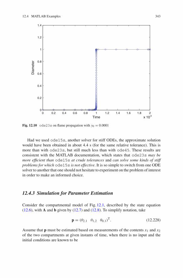
12.4 MATLAB Examples 343

0 0.2 0.4 0.6 0.8 1 1.2 1.4 1.6 1.8 2

x 104

0

0.2

0.4

0.6

0.8

1

1.2

1.4

Time

Dia

met

er

Fig. 12.10 ode23s on flame propagation with y0 = 0.0001

Had we used ode15s, another solver for stiff ODEs, the approximate solutionwould have been obtained in about 4.4 s (for the same relative tolerance). This ismore than with ode23s, but still much less than with ode45. These results areconsistent with the MATLAB documentation, which states that ode23s may bemore efficient than ode15s at crude tolerances and can solve some kinds of stiffproblems for which ode15s is not effective. It is so simple to switch from one ODEsolver to another that one should not hesitate to experiment on the problem of interestin order to make an informed choice.

12.4.3 Simulation for Parameter Estimation

Consider the compartmental model of Fig. 12.1, described by the state equation(12.6), with A and b given by (12.7) and (12.8). To simplify notation, take

p = (∂2,1 ∂1,2 ∂0,1)T. (12.228)

Assume that p must be estimated based on measurements of the contents x1 and x2of the two compartments at given instants of time, when there is no input and theinitial conditions are known to be

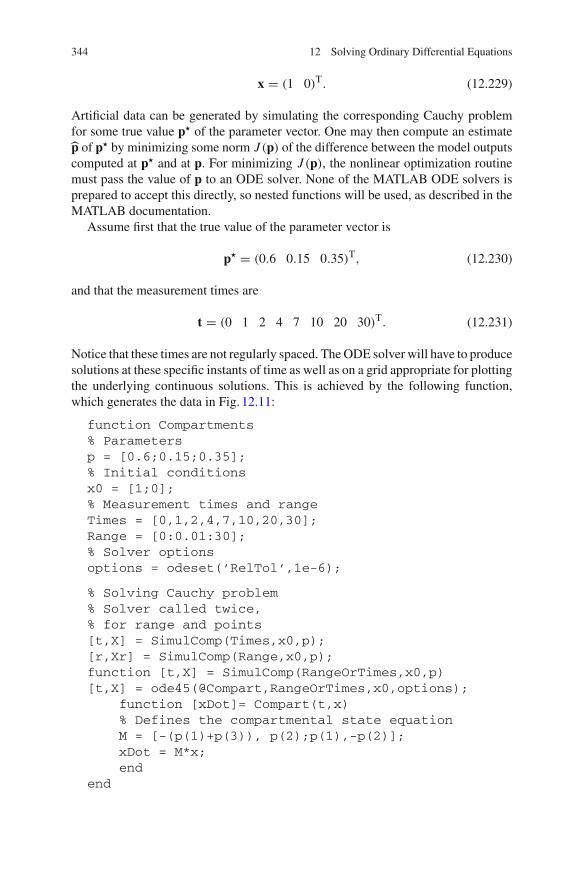
344 12 Solving Ordinary Differential Equations

x = (1 0)T. (12.229)

Artificial data can be generated by simulating the corresponding Cauchy problemfor some true value p� of the parameter vector. One may then compute an estimatep of p� by minimizing some norm J (p) of the difference between the model outputscomputed at p� and at p. For minimizing J (p), the nonlinear optimization routinemust pass the value of p to an ODE solver. None of the MATLAB ODE solvers isprepared to accept this directly, so nested functions will be used, as described in theMATLAB documentation.

Assume first that the true value of the parameter vector is

p� = (0.6 0.15 0.35)T, (12.230)

and that the measurement times are

t = (0 1 2 4 7 10 20 30)T. (12.231)

Notice that these times are not regularly spaced. The ODE solver will have to producesolutions at these specific instants of time as well as on a grid appropriate for plottingthe underlying continuous solutions. This is achieved by the following function,which generates the data in Fig. 12.11:

function Compartments% Parametersp = [0.6;0.15;0.35];% Initial conditionsx0 = [1;0];% Measurement times and rangeTimes = [0,1,2,4,7,10,20,30];Range = [0:0.01:30];% Solver optionsoptions = odeset(’RelTol’,1e-6);

% Solving Cauchy problem% Solver called twice,% for range and points[t,X] = SimulComp(Times,x0,p);[r,Xr] = SimulComp(Range,x0,p);function [t,X] = SimulComp(RangeOrTimes,x0,p)[t,X] = ode45(@Compart,RangeOrTimes,x0,options);

function [xDot]= Compart(t,x)% Defines the compartmental state equationM = [-(p(1)+p(3)), p(2);p(1),-p(2)];xDot = M*x;end

end

12.4 MATLAB Examples 345

0 5 10 15 20 25 300

0.1

0.2

0.3

0.4

0.5

0.6

0.7

0.8

0.9

1

Time

Sta

te

x1x2

Fig. 12.11 Data generated for the compartmental model of Fig. 12.1 by ode45 for x(0) = (1, 0)T

and p� = (0.6, 0.15, 0.35)T

% Plotting resultsfigure;hold onplot(t,X(:,1),’ks’);plot(t,X(:,2),’ko’);plot(r,Xr(:,1));plot(r,Xr(:,2));legend(’x_1’,’x_2’);ylabel(’State’);xlabel(’Time’)end

Assume now that the true value of the parameter vector is

p� = (0.6 0.35 0.15)T, (12.232)

which corresponds to exchanging the values of p�2 and p�

3. Compartments nowproduces the data described by Fig. 12.12.

While the solutions for x1 are quite different in Figs. 12.11 and 12.12, the solutionsfor x2 are extremely similar, as confirmed by Fig. 12.13 with corresponds to theirdifference.

This is actually not surprising, because an identifiability analysis [55] would showthat the parameters of this model cannot be estimated uniquely from measurementscarried out on x2 alone, as exchanging the role of p2 and p3 always leaves the solutionfor x2 unchanged. See also Sect. 16.22. Had we tried to estimate p with any of the

346 12 Solving Ordinary Differential Equations

0 5 10 15 20 25 300

0.1

0.2

0.3

0.4

0.5

0.6

0.7

0.8

0.9

1

Time

Sta

te

x1x2

Fig. 12.12 Data generated for the compartmental model of Fig. 12.1 by ode45 for x(0) = (1, 0)T

and p� = (0.6, 0.35, 0.15)T

methods for nonlinear optimization presented in Chap. 9 from artificial noise-freedata on x2 alone, we would have converged to an approximation of p� as given by(12.230) or (12.232) depending on our initialization. Multistart should have made itpossible to detect that there are two global minimizers, both associated with a verysmall value of the minimum.

12.4.4 Boundary Value Problem

A high-temperature pressurized fluid circulates in a long, thick, straight pipe. Weconsider a cross-section of this pipe, located far from its ends. Rotational symmetrymakes it possible to study the stationary distribution of temperatures along a radiusof this cross-section. The inner radius of the pipe is rin = 1 cm, and the outer radiusrout = 2 cm. The temperature (in ≈C) at radius r (in cm), denoted by T (r), is assumedto satisfy

d2T

dr2 = −1

r

dT

dr, (12.233)

and the boundary conditions are

12.4 MATLAB Examples 347

0 5 10 15 20 25 30−2

−1.5

−1

−0.5

0

0.5

1

1.5

2x 10

−7

Diff

eren

ce o

n x 2

Time

Fig. 12.13 Difference between the solutions for x2 when p� = (0.6, 0.15, 0.35)T and when p� =(0.6, 0.35, 0.15)T, as computed by ode45

T (1) = 100 and T (2) = 20. (12.234)

Equation (12.233) can be put in the state-space form

dxdr

= f(x, r), (12.235)

T (r) = g(x(r)), (12.236)

with x(r) = (T (r), T (r))T,

f(x, r) =[

0 10 − 1

r

⎡x(r) (12.237)

andg(x(r)) = (1 0)x(r), (12.238)

and the boundary conditions become

x1(1) = 100 and x1(2) = 20. (12.239)

348 12 Solving Ordinary Differential Equations

This BVP can be solved analytically, which provides the reference solution to whichthe solutions obtained by numerical methods will be compared.

12.4.4.1 Computing the Analytical Solution

It is easy to show thatT (r) = p1 ln(r) + p2, (12.240)

with p1 and p2 specified by the boundary conditions and obtained by solving thelinear system [

ln(rin) 1ln(rout) 1

⎡ [p1p2

⎡=

[T (rin)

T (rout)

⎡. (12.241)

The following script evaluates and plots the analytical solution on a regular grid fromr = 1 to r = 2 as

Radius = (1:0.01:2);A = [log(1),1;log(2),1];b = [100;20];p = A\b;MathSol = p(1)*log(Radius)+p(2);figure;plot(Radius,MathSol)xlabel(’Radius’)ylabel(’Temperature’)

It yields Fig. 12.14. The numerical methods used in Sects. 12.4.4.2–12.4.4.4 for solv-ing this BVP produce plots that are visually indistinguishable from Fig. 12.14, so theerrors between the numerical and analytical solutions will be plotted instead.

12.4.4.2 Using a Shooting Method

To compute the distribution of temperatures between rin and rout by a shootingmethod, we parametrize the second entry of the state at rin as p. For any given valueof p, computing the distribution of temperatures in the pipe is a Cauchy problem.The following script looks for pHat, the value of p that minimizes the square of thedeviation between the known temperature at rout and the one computed by ode45,and compares the resulting temperature profile to the analytical one obtained inSect. 12.4.4.1. It produces Fig. 12.15.

% Solving pipe problem by shootingclear allp0 = -50; % Initial guess for x_2(1)pHat = fminsearch(@PipeCost,p0)

12.4 MATLAB Examples 349

1 1.1 1.2 1.3 1.4 1.5 1.6 1.7 1.8 1.9 220

30

40

50

60

70

80

90

100

Radius

Tem

pera

ture

Fig. 12.14 Distribution of temperatures in the pipe, as computed analytically

% Comparing with mathematical solutionX1 = [100;pHat];[Radius, SolByShoot] = ...

ode45(@PipeODE,[1,2],X1);A = [log(1),1;log(2),1];b = [100;20];p = A\b;MathSol = p(1)*log(Radius)+p(2);Error = MathSol-SolByShoot(:,1);

% Plotting errorfigure;plot(Radius,Error)xlabel(’Radius’)ylabel(’Error on temperature of the shooting method’)

The ODE (12.235) is implemented in the function

function [xDot] = PipeODE(r,x)xDot = [x(2); -x(2)/r];end

The function

350 12 Solving Ordinary Differential Equations

1 1.1 1.2 1.3 1.4 1.5 1.6 1.7 1.8 1.9 2−2.5

−2

−1.5

−1

−0.5

0

0.5x 10

−5

Radius

Err

or o

n te

mpe

ratu

re o

f the

sho

otin

g m

etho

d

Fig. 12.15 Error on the distribution of temperatures in the pipe, as computed by the shootingmethod

function [r,X] = SimulPipe(p)X1 = [100;p];[r,X] = ode45(@PipeODE,[1,2],X1);end

is used to solve the Cauchy problem once the value of x2(1) = T (rin) has been setto p and the function

function [Cost] = PipeCost(p)[Radius,X] = SimulPipe(p);Cost = (20 - X(length(X),1))ˆ2;end

evaluates the cost to be minimized by fminsearch.

12.4.4.3 Using Finite Differences

To compute the distribution of temperatures between rin and rout with a finite-difference method, it suffices to specialize (12.184) into (12.233), which meanstaking

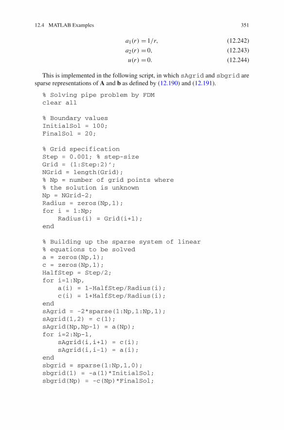
12.4 MATLAB Examples 351

a1(r) = 1/r, (12.242)

a2(r) = 0, (12.243)

u(r) = 0. (12.244)

This is implemented in the following script, in which sAgrid and sbgrid aresparse representations of A and b as defined by (12.190) and (12.191).

% Solving pipe problem by FDMclear all

% Boundary valuesInitialSol = 100;FinalSol = 20;

% Grid specificationStep = 0.001; % step-sizeGrid = (1:Step:2)’;NGrid = length(Grid);% Np = number of grid points where% the solution is unknownNp = NGrid-2;Radius = zeros(Np,1);for i = 1:Np;

Radius(i) = Grid(i+1);end

% Building up the sparse system of linear% equations to be solveda = zeros(Np,1);c = zeros(Np,1);HalfStep = Step/2;for i=1:Np,

a(i) = 1-HalfStep/Radius(i);c(i) = 1+HalfStep/Radius(i);

endsAgrid = -2*sparse(1:Np,1:Np,1);sAgrid(1,2) = c(1);sAgrid(Np,Np-1) = a(Np);for i=2:Np-1,

sAgrid(i,i+1) = c(i);sAgrid(i,i-1) = a(i);

endsbgrid = sparse(1:Np,1,0);sbgrid(1) = -a(1)*InitialSol;sbgrid(Np) = -c(Np)*FinalSol;

352 12 Solving Ordinary Differential Equations

% Solving the sparse system of linear equationspgrid = sAgrid\sbgrid;SolByFD = zeros(NGrid,1);SolByFD(1) = InitialSol;SolByFD(NGrid) = FinalSol;for i = 1:Np,

SolByFD(i+1) = pgrid(i);end

% Comparing with mathematical solutionA = [log(1),1;log(2),1];b = [100;20];p = A\b;MathSol = p(1)*log(Grid)+p(2);Error = MathSol-SolByFD;

% Plotting errorfigure;plot(Grid,Error)xlabel(’Radius’)ylabel(’Error on temperature of the FDM’)

This script yields Fig. 12.16.

Remark 12.19 We took advantage of the sparsity of A, but not from the fact that itis tridiagonal. With a step-size equal to 10−3 as in this script, a dense representationof A would have 106 entries. �

12.4.4.4 Using Collocation

Details on the principles and examples of use of the collocation solver bvp4c can befound in [9, 50]. The ODE (12.235) is still described by the function PipeODE, andthe errors on the satisfaction of the initial and final boundary conditions are evaluatedby the function

function [ResidualsOnBounds] = ...PipeBounds(xa,xb)

ResidualsOnBounds = [xa(1) - 100xb(1) - 20];

end

An initial guess for the solution must be provided to the solver. The following scriptguesses that the solution is identically zero on [1, 2]. The helper function bvpinitis then in charge of building a structure corresponding to this daring hypothesis before

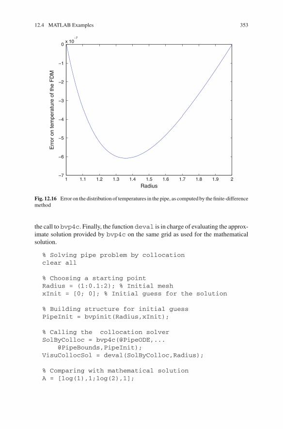
12.4 MATLAB Examples 353

1 1.1 1.2 1.3 1.4 1.5 1.6 1.7 1.8 1.9 2−7

−6

−5

−4

−3

−2

−1

0x 10

−7

Radius

Err

or o

n te

mpe

ratu

re o

f the

FD

M

Fig. 12.16 Error on the distribution of temperatures in the pipe, as computed by the finite-differencemethod

the call to bvp4c. Finally, the function deval is in charge of evaluating the approx-imate solution provided by bvp4c on the same grid as used for the mathematicalsolution.

% Solving pipe problem by collocationclear all

% Choosing a starting pointRadius = (1:0.1:2); % Initial meshxInit = [0; 0]; % Initial guess for the solution

% Building structure for initial guessPipeInit = bvpinit(Radius,xInit);

% Calling the collocation solverSolByColloc = bvp4c(@PipeODE,...

@PipeBounds,PipeInit);VisuCollocSol = deval(SolByColloc,Radius);

% Comparing with mathematical solutionA = [log(1),1;log(2),1];

354 12 Solving Ordinary Differential Equations

1 1.1 1.2 1.3 1.4 1.5 1.6 1.7 1.8 1.9 20

1

2

3

4

5

6x 10

−4

Radius

Err

or o

n te

mpe

ratu

re o

f the

col

loca

tion

met

hod

Fig. 12.17 Error on the distribution of temperatures in the pipe, computed by the collocationmethod as implemented in bvp4c with RelTol = 10−3

b = [100;20];p = A\b;MathSol = p(1)*log(Radius)+p(2);Error = MathSol-VisuCollocSol(1,:);

% Plotting errorfigure;plot(Radius,Error)xlabel(’Radius’)ylabel(’Error on temperature of the collocationmethod’)

The results are in Fig. 12.17. A more accurate solution can be obtained by decreasingthe relative tolerance from its default value of 10−3 (one could also make a moreeducated guess to be passed to bvp4c by bvpinit). By just replacing the call tobvp4c in the previous script by

optionbvp = bvpset(’RelTol’,1e-6)SolByColloc = bvp4c(@PipeODE,...

@PipeBounds,PipeInit,optionbvp);

we get the results in Fig. 12.18.

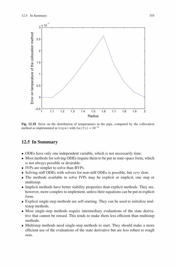
12.5 In Summary 355

1 1.1 1.2 1.3 1.4 1.5 1.6 1.7 1.8 1.9 2−0.5

0

0.5

1

1.5

2

2.5

3x 10

−7

Radius

Err

or o

n te

mpe

ratu

re o

f the

col

loca

tion

met

hod

Fig. 12.18 Error on the distribution of temperatures in the pipe, computed by the collocationmethod as implemented in bvp4c with RelTol = 10−6

12.5 In Summary

• ODEs have only one independent variable, which is not necessarily time.• Most methods for solving ODEs require them to be put in state-space form, which

is not always possible or desirable.• IVPs are simpler to solve than BVPs.• Solving stiff ODEs with solvers for non-stiff ODEs is possible, but very slow.• The methods available to solve IVPs may be explicit or implicit, one step or

multistep.• Implicit methods have better stability properties than explicit methods. They are,

however, more complex to implement, unless their equations can be put in explicitform.

• Explicit single-step methods are self-starting. They can be used to initialize mul-tistep methods.

• Most single-step methods require intermediary evaluations of the state deriva-tive that cannot be reused. This tends to make them less efficient than multistepmethods.

• Multistep methods need single-step methods to start. They should make a moreefficient use of the evaluations of the state derivative but are less robust to roughseas.

356 12 Solving Ordinary Differential Equations

• It is often useful to adapt step-size along the state trajectory, which is easy withsingle-step methods.

• It is often useful to adapt method order along the state trajectory, which is easywith multistep methods.

• The solution of BVPs may be via shooting methods and the minimization of anorm of the deviation of the solution from the boundary conditions, provided thatthe ODE is stable.

• Finite-difference methods do not require the ODEs to be put in state-space form.They can be used to solve IVPs and BVPs. An important ingredient is the solutionof (large, sparse) systems of linear equations.

• The projection approaches are based on finite-dimensional approximations of theODE. The free parameters of these approximations are evaluated by solving asystem of equations (collocation and Ritz-Galerkin approaches) or by minimizinga quadratic cost function (least-squares approach).

• Understanding finite-difference and projection approaches for ODEs should facil-itate the study of the same techniques for PDEs.

References

1. Higham, D.: An algorithmic introduction to numerical simulation of stochastic differentialequations. SIAM Rev. 43(3), 525–546 (2001)

2. Gear, C.: Numerical Initial Value Problems in Ordinary Differential Equations. Prentice-Hall,Englewood Cliffs (1971)

3. Stoer, J., Bulirsch, R.: Introduction to Numerical Analysis. Springer, New York (1980)4. Gupta, G., Sacks-Davis, R., Tischer, P.: A review of recent developments in solving ODEs.

ACM Comput. Surv. 17(1), 5–47 (1985)5. Shampine, L.: Numerical Solution of Ordinary Differential Equations. Chappman & Hall, New

York (1994)6. Shampine, L., Reichelt, M.: The MATLAB ODE suite. SIAM J. Sci. Comput. 18(1), 1–22

(1997)7. Shampine, L.: Vectorized solution of ODEs in MATLAB. Scalable Comput. Pract. Exper.

10(4), 337–345 (2009)8. Ashino, R., Nagase, M., Vaillancourt, R.: Behind and beyond the Matlab ODE suite. Comput.

Math. Appl. 40, 491–512 (2000)9. Shampine, L., Kierzenka, J., Reichelt, M.: Solving boundary value problems for ordinary

differential equations in MATLAB with bvp4c. http://www.mathworks.com/ (2000)10. Shampine, L., Gladwell, I., Thompson, S.: Solving ODEs in MATLAB. Cambridge University

Press, Cambridge (2003)11. Moler, C.: Numerical Computing with MATLAB, revised reprinted edn. SIAM, Philadelphia

(2008)12. Jacquez, J.: Compartmental Analysis in Biology and Medicine. BioMedware, Ann Arbor (1996)13. Gladwell, I., Shampine, L., Brankin, R.: Locating special events when solving ODEs. Appl.

Math. Lett. 1(2), 153–156 (1988)14. Shampine, L., Thompson, S.: Event location for ordinary differential equations. Comput. Math.

Appl. 39, 43–54 (2000)15. Moler, C., Van Loan, C.: Nineteen dubious ways to compute the exponential of a matrix,

twenty-five years later. SIAM Rev. 45(1), 3–49 (2003)

References 357

16. Al-Mohy, A., Higham, N.: A new scaling and squaring algorithm for the matrix exponential.SIAM J. Matrix Anal. Appl. 31(3), 970–989 (2009)

17. Higham, N.: The scaling and squaring method for the matrix exponential revisited. SIAM Rev.51(4), 747–764 (2009)

18. Butcher, J., Wanner, G.: Runge-Kutta methods: some historical notes. Appl. Numer. Math. 22,113–151 (1996)

19. Alexander, R.: Diagonally implicit Runge-Kutta methods for stiff O.D.E’.s. SIAM J. Numer.Anal. 14(6), 1006–1021 (1977)

20. Butcher, J.: Implicit Runge-Kutta processes. Math. Comput. 18(85), 50–64 (1964)21. Steihaug T, Wolfbrandt A.: An attempt to avoid exact Jacobian and nonlinear equations in the

numerical solution of stiff differential equations. Math. Comput. 33(146):521–534 (1979)22. Zedan, H.: Modified Rosenbrock-Wanner methods for solving systems of stiff ordinary differ-

ential equations. Ph.D. thesis, University of Bristol, Bristol, UK (1982)23. Moore, R.: Mathematical Elements of Scientific Computing. Holt, Rinehart and Winston, New

York (1975)24. Moore, R.: Methods and Applications of Interval Analysis. SIAM, Philadelphia (1979)25. Bertz, M., Makino, K.: Verified integration of ODEs and flows using differential algebraic

methods on high-order Taylor models. Reliable Comput. 4, 361–369 (1998)26. Makino, K., Bertz, M.: Suppression of the wrapping effect by Taylor model-based verified

integrators: long-term stabilization by preconditioning. Int. J. Differ. Equ. Appl. 10(4), 353–384 (2005)

27. Makino, K., Bertz, M.: Suppression of the wrapping effect by Taylor model-based verifiedintegrators: the single step. Int. J. Pure Appl. Math. 36(2), 175–196 (2007)

28. Klopfenstein, R.: Numerical differentiation formulas for stiff systems of ordinary differentialequations. RCA Rev. 32, 447–462 (1971)

29. Shampine, L.: Error estimation and control for ODEs. J. Sci. Comput. 25(1/2), 3–16 (2005)30. Dahlquist, G.: A special stability problem for linear multistep methods. BIT Numer. Math.

3(1), 27–43 (1963)31. LeVeque, R.: Finite Difference Methods for Ordinary and Partial Differential Equations. SIAM,

Philadelphia (2007)32. Hairer, E., Wanner, G.: On the instability of the BDF formulas. SIAM J. Numer. Anal. 20(6),

1206–1209 (1983)33. Mathews, J., Fink, K.: Numerical Methods Using MATLAB, 4th edn. Prentice-Hall, Upper

Saddle River (2004)34. Bogacki, P., Shampine, L.: A 3(2) pair of Runge-Kutta formulas. Appl. Math. Lett. 2(4), 321–

325 (1989)35. Dormand, J., Prince, P.: A family of embedded Runge-Kutta formulae. J. Comput. Appl. Math.

6(1), 19–26 (1980)36. Prince, P., Dormand, J.: High order embedded Runge-Kutta formulae. J. Comput. Appl. Math.

7(1), 67–75 (1981)37. Dormand, J., Prince, P.: A reconsideration of some embedded Runge-Kutta formulae. J. Com-

put. Appl. Math. 15, 203–211 (1986)38. Shampine, L.: What everyone solving differential equations numerically should know. In:

Gladwell, I., Sayers, D. (eds.): Computational Techniques for Ordinary Differential Equations.Academic Press, London (1980)

39. Skufca, J.: Analysis still matters: A surprising instance of failure of Runge-Kutta-Felberg ODEsolvers. SIAM Rev. 46(4), 729–737 (2004)

40. Shampine, L., Gear, C.: A user’s view of solving stiff ordinary differential equations. SIAMRev. 21(1), 1–17 (1979)

41. Segel, L., Slemrod, M.: The quasi-steady-state assumption: A case study in perturbation. SIAMRev. 31(3), 446–477 (1989)

42. Duchêne, P., Rouchon, P.: Kinetic sheme reduction, attractive invariant manifold and slow/fastdynamical systems. Chem. Eng. Sci. 53, 4661–4672 (1996)

358 12 Solving Ordinary Differential Equations

43. Boulier, F., Lefranc, M., Lemaire, F., Morant, P.E.: Model reduction of chemical reactionsystems using elimination. Math. Comput. Sci. 5, 289–301 (2011)

44. Petzold, L.: Differential/algebraic equations are not ODE’s. SIAM J. Sci. Stat. Comput. 3(3),367–384 (1982)

45. Reddien, G.: Projection methods for two-point boundary value problems. SIAM Rev. 22(2),156–171 (1980)

46. de Boor, C.: Package for calculating with B-splines. SIAM J. Numer. Anal. 14(3), 441–472(1977)

47. Farouki, R.: The Bernstein polynomial basis: a centennial retrospective. Comput. Aided Geom.Des. 29, 379–419 (2012)

48. Bhatti, M., Bracken, P.: Solution of differential equations in a Bernstein polynomial basis. J.Comput. Appl. Math. 205, 272–280 (2007)

49. Russel, R., Shampine, L.: A collocation method for boundary value problems. Numer. Math.19, 1–28 (1972)

50. Kierzenka, J., Shampine, L.: A BVP solver based on residual control and the MATLAB PSE.ACM Trans. Math. Softw. 27(3), 299–316 (2001)

51. Gander, M., Wanner, G.: From Euler, Ritz, and Galerkin to modern computing. SIAM Rev.54(4), 627–666 (2012)

52. Lotkin, M.: The treatment of boundary problems by matrix methods. Am. Math. Mon. 60(1),11–19 (1953)

53. Russell, R., Varah, J.: A comparison of global methods for linear two-point boundary valueproblems. Math. Comput. 29(132), 1007–1019 (1975)

54. de Boor, C., Swartz, B.: Comments on the comparison of global methods for linear two-pointboudary value problems. Math. Comput. 31(140):916–921 (1977)

55. Walter, E.: Identifiability of State Space Models. Springer, Berlin (1982)

Chapter 13Solving Partial Differential Equations

13.1 Introduction

Contrary to the ordinary differential equations (or ODEs) considered in Chap. 12,partial differential equations (or PDEs) involve more than one independent variable.Knowledge-based models of physical systems typically involve PDEs (Maxwell’sin electromagnetism, Schrödinger’s in quantum mechanics, Navier–Stokes’ in fluiddynamics, Fokker–Planck’s in statistical mechanics, etc.). It is only in very specialsituations that PDEs simplify into ODEs. In chemical engineering, for example,concentrations of chemical species generally obey PDEs. It is only in continuousstirred tank reactors (CSTRs) that they can be considered as position-independentand that time becomes the only independent variable.

The study of the mathematical properties of PDEs is considerably more involvedthan for ODEs. Proving, for instance, the existence and smoothness of Navier–Stokessolutions on R

3 (or giving a counterexample) would be one of the achievements forwhich the Clay Mathematics Institute is ready, since May 2000, to attribute one ofits seven one-million-dollar Millennium Prizes.

This chapter will just scratch the surface of PDE simulation. Good starting pointsto go further are [1], which addresses the modeling of real-life problems, the analysisof the resulting PDE models and their numerical simulation via a finite-differenceapproach, [2], which develops many finite-difference schemes with applications incomputational fluid dynamics and [3], where finite-difference and finite-elementmethods are both considered. Each of these books treats many examples in detail.

13.2 Classification

The methods for solving PDEs depend, among other things, on whether they are linearor not, on their order, and on the type of boundary conditions being considered.

É. Walter, Numerical Methods and Optimization, 359DOI: 10.1007/978-3-319-07671-3_13,© Springer International Publishing Switzerland 2014

360 13 Solving Partial Differential Equations

13.2.1 Linear and Nonlinear PDEs

As with ODEs, an important special case is when the dependent variables and theirpartial derivatives with respect to the independent variables enter the PDE linearly.The scalar wave equation in two space dimensions

∂2 y

∂t2 = c2

(∂2 y

∂x21

+ ∂2 y

∂x22

⎡, (13.1)

where y(t, x) specifies a displacement at time t and point x = (x1, x2)T in a 2D

space and where c is the propagation speed, is thus a linear PDE. Its independentvariables are t, x1 and x2, and its dependent variable is y. The superposition principleapplies to linear PDEs, so the sum of two solutions is a solution. The coefficients inlinear PDEs may be functions of the independent variables, but not of the dependentvariables.

The viscous Burgers equation of fluid mechanics

∂y

∂t+ y

∂y

∂x= ν

∂2 y

∂x2 , (13.2)

where y(t, x) is the fluid velocity and ν its viscosity, is nonlinear, as the second termin its left-hand side involves the product of y by its partial derivative with respectto x .

13.2.2 Order of a PDE

The order of a single scalar PDE is that of the highest-order derivative of the dependentvariable with respect to the independent variables. Thus, (13.2) is a second-order PDEexcept when ν = 0, which corresponds to the first-order inviscid Burgers equation

∂y

∂t+ y

∂y

∂x= 0. (13.3)

As with ODEs, a scalar PDE may be decomposed in a system of first-order PDEs.The order of this system is then that of the single scalar PDE obtained by combiningall of them.

13.2 Classification 361

Example 13.1 The system of three first-order PDEs

∂u

∂x1+ ∂v

∂x2= ∂u

∂t,

u = ∂y

∂x1,

v = ∂y

∂x2(13.4)

is equivalent to∂2 y

∂x21

+ ∂2 y

∂x22

= ∂2 y

∂t∂x1. (13.5)

Its order is thus two. �

13.2.3 Types of Boundary Conditions

As with ODEs, boundary conditions are required to specify the solutions(s) of interestof the PDE, and we assume that these boundary conditions are such that there is atleast one such solution.

• Dirichlet conditions specify values of the solution y on the boundary ∂D of thedomain D under study. This may correspond, e.g., to a potential at the surface ofan electrode, a temperature at one end of a rod or the position of a fixed end of avibrating string.

• Neumann conditions specify values of the flux ∂y∂n of the solution through ∂D, with

n a vector normal to ∂D. This may correspond, e.g., to the injection of an electriccurrent into a system.

• Robin conditions are linear combinations of Dirichlet and Neumann conditions.• Mixed boundary conditions are such that a Dirichlet condition applies to some part

of ∂D and a Neumann condition to another part of ∂D.

13.2.4 Classification of Second-Order Linear PDEs

Second-order linear PDEs are important enough to receive a classification of theirown. We assume here, for the sake of simplicity, that there are only two independentvariables t and x and that the solution y(t, x) is scalar. The first of these indepen-dent variables may be associated with time and the second with space, but otherinterpretations are of course possible.

Remark 13.1 Often, x becomes a vector x, which may specify position in some2D or 3D space, and the solution y also becomes a vector y(t, x), because one is

362 13 Solving Partial Differential Equations

interested, for instance, in the temperature and chemical composition at time t andspace coordinates specified by x in a plug-flow reactor. Such problems, which involveseveral domains of physics and chemistry (here, fluid mechanics, thermodynamics,and chemical kinetics), pertain to what is called multiphysics. �

To simplify notation, we write

yx ≡ ∂y

∂x, yxx ≡ ∂2 y

∂x2 , yxt ≡ ∂2 y

∂x∂t, (13.6)

and so forth. The Laplacian operator, for instance, is then such that

δy = ytt + yxx . (13.7)

All the PDEs considered here can be written as

aytt + 2bytx + cyxx = g(t, x, y, yt , yx ). (13.8)

Since the solutions should also satisfy

dyt = ytt dt + ytx dx, (13.9)

dyx = yxt dt + yxx dx, (13.10)

where yxt = ytx , the following system of linear equations must hold true

M

⎢

⎣ytt

ytx

yxx

⎤

⎥ =⎢

⎣g(t, x, y, yt , yx )

dyt

dyx

⎤

⎥ , (13.11)

where

M =⎢

⎣a 2b cdt dx 00 dt dx

⎤

⎥ . (13.12)

The solution y(t, x) is assumed to be once continuously differentiable with respectto t and x . Discontinuities may appear in the second derivatives when det M = 0,i.e., when

a(dx)2 − 2b(dx)(dt) + c(dt)2 = 0. (13.13)

Divide (13.13) by (dt)2 to get

a

⎦dx

dt

⎞2

− 2b

⎦dx

dt

⎞+ c = 0. (13.14)

The solutions of this equation are such that

13.2 Classification 363

dx

dt= b ± √

b2 − ac

a. (13.15)

They define the characteristic curves of the PDE. The number of real solutionsdepends on the sign of the discriminant b2 − ac.

• When b2 − ac < 0, there is no real characteristic curve and the PDE is elliptic,• When b2 − ac = 0, there is a single real characteristic curve and the PDE is

parabolic,• When b2 − ac > 0, there are two real characteristic curves and the PDE is hyper-

bolic.

This classification depends only on the coefficients of the highest-order derivativesin the PDE. The qualifiers of these three types of PDEs have been chosen becausethe quadratic equation

a(dx)2 − 2b(dx)(dt) + c(dt)2 = constant (13.16)

defines an ellipse in (dx, dt) space if b2 − ac < 0, a parabola if b2 − ac = 0 and ahyperbola if b2 − ac > 0.

Example 13.2 Laplace’s equation in electrostatics

ytt + yxx = 0, (13.17)

with y a potential, is elliptic. The heat equation

cyxx = yt , (13.18)

with y a temperature, is parabolic. The vibrating-string equation

aytt = yxx , (13.19)

with y a displacement, is hyperbolic. The equation

ytt + (t2 + x2 − 1)yxx = 0 (13.20)

is elliptic outside the unit circle centered at (0, 0), and hyperbolic inside. �

Example 13.3 Aircraft flying at Mach 0.7 will be heard by ground observerseverywhere around, and the PDE describing sound propagation during such a sub-sonic flight is elliptic. When speed is increased to Mach 1, a front develops ahead ofwhich the noise is no longer heard; this front corresponds to a single real characteris-tic curve, and the PDE describing sound propagation during sonic flight is parabolic.When speed is increased further, the noise is only heard within Mach lines, whichform a pair of real characteristic curves, and the PDE describing sound propagation

364 13 Solving Partial Differential Equations

Space

Time

ht

hx

Fig. 13.1 Regular grid

during supersonic flight is hyperbolic. The real characteristic curves, if any, thuspatch radically different solutions. �

13.3 Finite-Difference Method

As with ODEs, the basic idea of the finite-difference method (FDM) is to replace theinitial PDE by an approximate equation linking the values taken by the approximatesolution at the nodes of a grid. The analytical and numerical aspects of the finite-difference approach to elliptic, parabolic, and hyperbolic problems are treated in [1],which devotes considerable attention to modeling issues and presents a number ofpractical applications. See also [2, 3].

We assume here that the grid on which the solution will be approximated is regular,and such that

tl = t1 + (l − 1)ht , (13.21)

xm = x1 + (m − 1)hx , (13.22)

as illustrated by Fig. 13.1. (This assumption could be relaxed.)

13.3 Finite-Difference Method 365

13.3.1 Discretization of the PDE

The procedure, similar to that used for ODEs in Sect. 12.3.3, is as follows:

1. Replace the partial derivatives in the PDE by finite-difference approximations,for instance,

yt (tl , xm) ≈ Yl,m − Yl−1,m

ht, (13.23)

yxx (tl , xm) ≈ Yl,m+1 − 2Yl,m + Yl,m−1

h2x

, (13.24)

with Yl,m the approximate value of y(tl , xm) to be computed.2. Write down the resulting discrete equations at all the grid points where this is

possible, taking into account the information provided by the boundary conditionswherever needed.

3. Solve the resulting system of equations for the Yl,m’s.

There are, of course, degrees of freedom in the choice of the finite-difference approx-imations of the partial derivatives. For instance, one may choose

yt (tl , xm) ≈ Yl,m − Yl−1,m

ht, (13.25)

yt (tl , xm) ≈ Yl+1,m − Yl,m

ht(13.26)

or

yt (tl , xm) ≈ Yl+1,m − Yl−1,m

2ht. (13.27)

These degrees of freedom can be taken advantage of to facilitate the propagation ofboundary information and mitigate the effect of method errors.

13.3.2 Explicit and Implicit Methods

Sometimes, computation can be ordered in such a way that the approximate solutionfor Yl,m at grid points where it is still unknown is a function of the known boundaryconditions and of values Yi, j already computed. It is then possible to obtain theapproximate solution at all the grid points by an explicit method, through a recurrenceequation. This is in contrast with implicit methods, where all the equations linkingall the Yl,m’s are considered simultaneously.

Explicit methods have two serious drawbacks. First, they impose constraints onthe step-sizes to ensure the stability of the recurrence equation. Second, the errors

366 13 Solving Partial Differential Equations

committed during the past steps of the recurrence impact the future steps. This iswhy one may avoid these methods even when they are feasible, and prefer implicitmethods.

For linear PDEs, implicit methods require the solution of large systems of linearequations

Ay = b, (13.28)

with y = vect(Yl,m). The difficulty is mitigated by the fact that A is sparse and oftendiagonally dominant, so iterative methods are particularly well suited, see Sect. 3.7.Because the size of A may be enormous, care should be exercised in its storage andin the indexation of the grid points, to avoid slowing down computation by accessesto disk memory that could have been avoided.

13.3.3 Illustration: The Crank–Nicolson Scheme

Consider the heat equation with a single space variable x .

∂y(t, x)

∂t= α 2 ∂2 y(t, x)

∂x2 . (13.29)

With the simplified notation, this parabolic equation becomes

cyxx = yt , (13.30)

where c = α 2.Take a first-order forward approximation of yt (tl , xm)

yt (tl , xm) ≈ Yl+1,m − Yl,m

ht. (13.31)

At the midpoint of the edge between the grid points indexed by (l, m) and (l +1, m),it becomes a second-order centered approximation

yt

⎦tl + ht

2, xm

⎞≈ Yl+1,m − Yl,m

ht. (13.32)

To take advantage of this increase in the order of method error, the Crank–Nicolsonscheme approximates (13.29) at such off-grid points (Fig. 13.2). The value of yxx atthe off-grid point indexed by (l + 1/2, m) is then approximated by the arithmeticmean of its values at the two adjacent grid points

yxx

⎦tl + ht

2, xm

⎞≈ 1

2

⎠yxx (tl+1, xm) + yxx (tl , xm)

], (13.33)

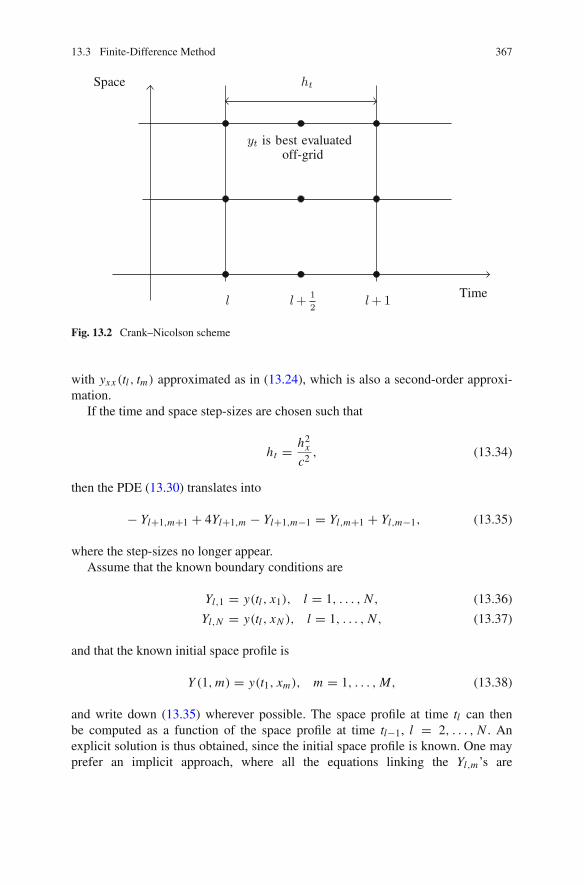
13.3 Finite-Difference Method 367

Space

Time

ht

off-gridyt is best evaluated

l+ 12

l+1l

Fig. 13.2 Crank–Nicolson scheme

with yxx (tl , tm) approximated as in (13.24), which is also a second-order approxi-mation.

If the time and space step-sizes are chosen such that

ht = h2x

c2 , (13.34)

then the PDE (13.30) translates into

− Yl+1,m+1 + 4Yl+1,m − Yl+1,m−1 = Yl,m+1 + Yl,m−1, (13.35)

where the step-sizes no longer appear.Assume that the known boundary conditions are

Yl,1 = y(tl , x1), l = 1, . . . , N , (13.36)

Yl,N = y(tl , xN ), l = 1, . . . , N , (13.37)

and that the known initial space profile is

Y (1, m) = y(t1, xm), m = 1, . . . , M, (13.38)

and write down (13.35) wherever possible. The space profile at time tl can thenbe computed as a function of the space profile at time tl−1, l = 2, . . . , N . Anexplicit solution is thus obtained, since the initial space profile is known. One mayprefer an implicit approach, where all the equations linking the Yl,m’s are

368 13 Solving Partial Differential Equations

considered simultaneously. The resulting system can be put in the form (13.28),with A tridiagonal, which simplifies solution considerably.

13.3.4 Main Drawback of the Finite-Difference Method

The main drawback of the FDM, which is also a strong argument in favor of theFEM presented next, is that a regular grid is often not flexible enough to adapt to thecomplexity of the boundary conditions encountered in some industrial applicationsas well as to the need to vary step-sizes when and where needed to get sufficientlyaccurate approximations. Research on grid generation has made the situation lessclear cut, however [2, 4].

13.4 A Few Words About the Finite-Element Method

The finite-element method (FEM) [5] is the main workhorse for the solution of PDEswith complicated boundary conditions as arise in actual engineering applications,e.g., in the aerospace industry. A detailed presentation of this method is out of thescope of this book, but the main similarities and differences with the FDM will bepointed out.

Because developing professional-grade, multiphysics finite-element software isparticularly complex, it is even more important than for simpler matters to know whatsoftware is already available, with its strengths and limitations. Many of the com-ponents of finite-element solvers should look familiar to the reader of the previouschapters.

13.4.1 FEM Building Blocks

13.4.1.1 Meshes

The domain of interest in the space of independent variables is partitioned into simplegeometric objects, for instance triangles in a 2D space or tetrahedrons in a 3D space.Computing this partition is called mesh generation, or meshing. In what follows,triangular meshes are used for illustration.

Meshes may be quite irregular, for at least two reasons:

1. it may be necessary to increase mesh density near the boundary of the domainof interest, in order to describe it more accurately,

2. increasing mesh density wherever the norm of the gradient of the solution isexpected to be large facilitates the obtention of more accurate solutions, just asadapting step-size makes sense when solving ODEs.

13.4 A Few Words About the Finite-Element Method 369

−1.5 −1 −0.5 0 0.5 1 1.5−1

−0.8

−0.6

−0.4

−0.2

0

0.2

0.4

0.6

0.8

1

Fig. 13.3 Mesh created by pdetool

Software is available to automate meshing for complex geometrical domains such asthose generated by computer-aided design, and meshing by hand is quite out of thequestion, even if one may have to modify some of the meshes generated automatically.

Figure 13.3 presents a mesh created in one click over an ellipsoidal domain usingthe graphical user interface pdetool of the MATLAB PDE Toolbox. A secondclick produces the refined mesh of Fig. 13.4. It is often more economical to let thePDE solver refine the mesh only where needed to get an accurate solution.

Remark 13.2 In shape optimization, automated mesh generation may have to beperformed at each iteration of the optimization algorithm, as the boundary of thedomain of interest changes. �

Remark 13.3 Real-life problems may involve billions of mesh vertices, and a properindexing of these vertices is crucial to avoid slowing down computation. �

13.4.1.2 Finite Elements

With each elementary geometric object of the mesh is associated a finite element,which approximates the solution on this object and is identically zero outside.(Splines, described in Sect. 5.3.2, may be viewed as finite elements on a mesh thatconsists of intervals. Each of these elements is polynomial on one interval and iden-tically zero on all the others.)

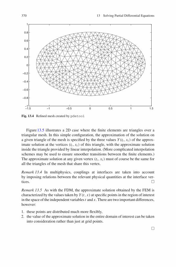
370 13 Solving Partial Differential Equations

−1.5 −1 −0.5 0 0.5 1 1.5−1

−0.8

−0.6

−0.4

−0.2

0

0.2

0.4

0.6

0.8

1

Fig. 13.4 Refined mesh created by pdetool

Figure 13.5 illustrates a 2D case where the finite elements are triangles over atriangular mesh. In this simple configuration, the approximation of the solution ona given triangle of the mesh is specified by the three values Y (ti , xi ) of the approx-imate solution at the vertices (ti , xi ) of this triangle, with the approximate solutioninside the triangle provided by linear interpolation. (More complicated interpolationschemes may be used to ensure smoother transitions between the finite elements.)The approximate solution at any given vertex (ti , xi ) must of course be the same forall the triangles of the mesh that share this vertex.

Remark 13.4 In multiphysics, couplings at interfaces are taken into accountby imposing relations between the relevant physical quantities at the interface ver-tices. �

Remark 13.5 As with the FDM, the approximate solution obtained by the FEM ischaracterized by the values taken by Y (t, x) at specific points in the region of interestin the space of the independent variables t and x . There are two important differences,however:

1. these points are distributed much more flexibly,2. the value of the approximate solution in the entire domain of interest can be taken

into consideration rather than just at grid points.

�

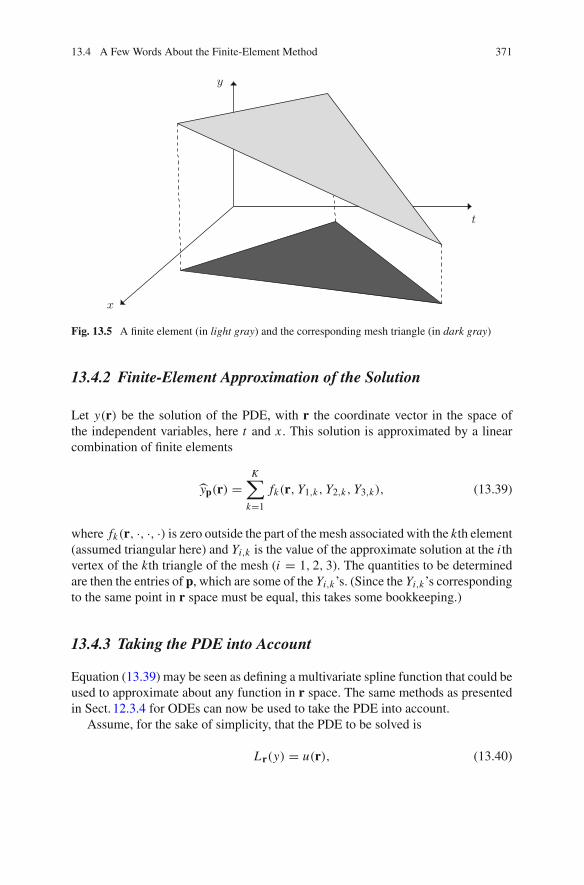
13.4 A Few Words About the Finite-Element Method 371

x

t

y

Fig. 13.5 A finite element (in light gray) and the corresponding mesh triangle (in dark gray)

13.4.2 Finite-Element Approximation of the Solution

Let y(r) be the solution of the PDE, with r the coordinate vector in the space ofthe independent variables, here t and x . This solution is approximated by a linearcombination of finite elements

yp(r) =K∑

k=1

fk(r, Y1,k, Y2,k, Y3,k), (13.39)

where fk(r, ·, ·, ·) is zero outside the part of the mesh associated with the kth element(assumed triangular here) and Yi,k is the value of the approximate solution at the i thvertex of the kth triangle of the mesh (i = 1, 2, 3). The quantities to be determinedare then the entries of p, which are some of the Yi,k’s. (Since the Yi,k’s correspondingto the same point in r space must be equal, this takes some bookkeeping.)

13.4.3 Taking the PDE into Account

Equation (13.39) may be seen as defining a multivariate spline function that could beused to approximate about any function in r space. The same methods as presentedin Sect. 12.3.4 for ODEs can now be used to take the PDE into account.

Assume, for the sake of simplicity, that the PDE to be solved is

Lr(y) = u(r), (13.40)

372 13 Solving Partial Differential Equations

where L(·) is a linear differential operator, Lr(y) is the value taken by L(y) at r, andu(r) is a known input function. Assume also that the solution y(r) is to be computedfor known Dirichlet boundary conditions on ∂D, with D some domain in r space.

To take these boundary conditions into account, rewrite (13.39) as

yp(r) = �T(r)p + ρ0(r), (13.41)

where ρ0(·) satisfies the boundary conditions, where

�(r) = 0, ∀r ∈ ∂D, (13.42)

and where p now corresponds to the parameters needed to specify the solution oncethe boundary conditions have been accounted for by ρ0(·).

Plug the approximate solution (13.41) in (13.40) to define the residual

ep(r) = Lr(yp

) − u(r), (13.43)

which is affine in p. The same projection methods as in Sect. 12.3.4 may be used totune p so as to make the residuals small.

13.4.3.1 Collocation

Collocation is the simplest of these approaches. As in Sect. 12.3.4.1, it imposes that

ep(ri ) = 0, i = 1, . . . , dim p, (13.44)

where the ri ’s are the collocation points. This yields a system of linear equations tobe solved for p.

13.4.3.2 Ritz–Galerkin Methods

With the Ritz–Galerkin methods, as in Sect. 12.3.4.2, p is obtained as the solution ofthe linear system

∫

D

ep(r)σi (r) dr = 0, i = 1, . . . , dim p, (13.45)

where σi (r) is a test function, which may be the i th entry of �(r). Collocation isobtained if σi (r) in (13.45) is replaced by ν(r − ri ), with ν(·) the Dirac measure.

13.4 A Few Words About the Finite-Element Method 373

13.4.3.3 Least Squares

As in Sect. 12.3.4.3, one may also minimize a quadratic cost function and choose

p = arg minp

∫

D

e2p(r) dr. (13.46)

Since ep(r) is affine in p, linear least squares may once again be used. The first-ordernecessary conditions for optimality then translate into a system of linear equationsthat p must satisfy.

Remark 13.6 For linear PDEs, each of the three approaches of Sect. 13.4.3yields a system of linear equations to be solved for p. This system will be sparseas each entry of p relates to a very small number of elements, but nonzero entriesmay turn out to be quite far from the main descending diagonal. Again, reindexingmay have to be carried out to avoid a potentially severe slowing down of thecomputation.

When the PDE is nonlinear, the collocation and Ritz–Galerkin methods requiresolving a system of nonlinear equations, whereas the least-squares solution isobtained by nonlinear programming. �

13.5 MATLAB Example

A stiffness-free vibrating string with length L satisfies

βytt = T yxx , (13.47)

where

• y(x, t) is the string elongation at location x and time t ,• β is the string linear density,• T is the string tension.

The string is attached at its two ends, so

y(0, t) ≡ y(L , t) ≡ 0. (13.48)

At t = 0, the string has the shape

y(x, 0) = sin(κx) ∀x ∈ [0, L], (13.49)

374 13 Solving Partial Differential Equations

and it is not moving, so

yt (x, 0) = 0 ∀x ∈ [0, L]. (13.50)

We define a regular grid on [0, tmax] × [0, L], such that (13.21) and (13.22) aresatisfied, and denote by Ym,l the approximation of y(xm, tl). Using the second-ordercentered difference ( 6.75), we take

ytt (xi , tn) ≈ Y (i, n + 1) − 2Y (i, n) + Y (i, n − 1)

h2t

(13.51)

and

yxx (xi , tn) ≈ Y (i + 1, n) − 2Y (i, n) + Y (i − 1, n)

h2x

, (13.52)

and replace (13.47) by the recurrence

Y (i, n + 1) − 2Y (i, n) + Y (i, n − 1)

h2t

= T

β

Y (i + 1, n) − 2Y (i, n) + Y (i − 1, n)

h2x

.

(13.53)With

R = T h2t

βh2x, (13.54)

this recurrence becomes

Y (i, n+1)+Y (i, n−1)−RY (i+1, n)−2(1−R)Y (i, n)−RY (i−1, n) = 0. (13.55)

Equation (13.49) translates into

Y (i, 1) = sin(κ(i − 1)hx ), (13.56)

and (13.50) intoY (i, 2) = Y (i, 1). (13.57)

The values of the approximate solution for y at all the grid points are stackedin a vector z that satisfies a linear system Az = b, where the contents of A and bare specified by (13.55) and the boundary conditions. After evaluating z, one mustunstack it to visualize the solution. This is achieved in the following script, whichproduces Figs. 13.6 and 13.7. A rough (and random) estimate of the condition numberof A for the 1-norm is provided by condest, and found to be approximately equalto 5,000, so this is not an ill-conditioned problem.

13.5 MATLAB Example 375

0 0.1 0.2 0.3 0.4 0.5 0.6 0.7 0.8 0.9 1−1

−0.8

−0.6

−0.4

−0.2

0

0.2

0.4

0.6

0.8

1

Location

Elo

ngat

ion

Fig. 13.6 2D visualization of the FDM solution for the string example

00.2

0.40.6

0.81

0

0.2

0.4

0.6

0.8

1−1

−0.5

0

0.5

1

TimeLocation

Elo

ngat

ion

Fig. 13.7 3D visualization of the FDM solution for the string example

376 13 Solving Partial Differential Equations

clear all

% String parametersL = 1; % LengthT = 4; % TensionRho = 1; % Linear density

% Discretization parametersTimeMax = 1; % Time horizonNx = 50; % Number of space stepsNt = 100; % Number of time stepshx = L/Nx; % Space step-sizeht = TimeMax/Nt; % Time step-size

% Creating sparse matrix A and vector b% full of zerosSizeA = (Nx+1)*(Nt+1);A = sparse(1:SizeA,1:SizeA,0);b = sparse(1:SizeA,1,0);

% Filling A and b (MATLAB indices cannot be zero)R = (T/Rho)*(ht/hx)ˆ2;Row = 0;for i=0:Nx,

Column=i+1;Row=Row+1;A(Row,Column)=1;b(Row)=sin(pi*i*hx/L);

endfor i=0:Nx,

DeltaCol=i+1;Row=Row+1;A(Row,(Nx+1)+DeltaCol)=1;b(Row)=sin(pi*i*hx/L);

endfor n=1:Nt-1,

DeltaCol=1;Row = Row+1;A(Row,(n+1)*(Nx+1)+DeltaCol)=1;for i=1:Nx-1

DeltaCol=i+1;Row = Row+1;A(Row,n*(Nx+1)+DeltaCol)=-2*(1-R);

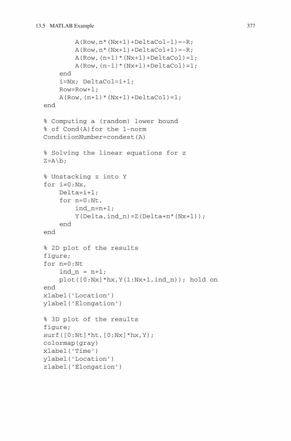
13.5 MATLAB Example 377

A(Row,n*(Nx+1)+DeltaCol-1)=-R;A(Row,n*(Nx+1)+DeltaCol+1)=-R;A(Row,(n+1)*(Nx+1)+DeltaCol)=1;A(Row,(n-1)*(Nx+1)+DeltaCol)=1;

endi=Nx; DeltaCol=i+1;Row=Row+1;A(Row,(n+1)*(Nx+1)+DeltaCol)=1;

end

% Computing a (random) lower bound% of Cond(A)for the 1-normConditionNumber=condest(A)

% Solving the linear equations for zZ=A\b;

% Unstacking z into Yfor i=0:Nx,

Delta=i+1;for n=0:Nt,

ind_n=n+1;Y(Delta,ind_n)=Z(Delta+n*(Nx+1));

endend

% 2D plot of the resultsfigure;for n=0:Nt

ind_n = n+1;plot([0:Nx]*hx,Y(1:Nx+1,ind_n)); hold on

endxlabel(’Location’)ylabel(’Elongation’)

% 3D plot of the resultsfigure;surf([0:Nt]*ht,[0:Nx]*hx,Y);colormap(gray)xlabel(’Time’)ylabel(’Location’)zlabel(’Elongation’)

378 13 Solving Partial Differential Equations

13.6 In Summary

• Contrary to ODEs, PDEs have several independent variables.• Solving PDEs is much more complex than solving ODEs.• As with ODEs, boundary conditions are needed to specify the solutions of PDEs.• The FDM for PDEs is based on the same principles as for ODEs.• The explicit FDM computes the solutions of PDEs by recurrence from profiles

specified by the boundary conditions. It is not always applicable, and the errorscommitted on past steps of the recurrence impact the future steps.

• The implicit FDM involves solving (large, sparse) systems of linear equations. Itavoids the cumulative errors of the explicit FDM.

• The FEM is more flexible than the FDM as regards boundary conditions. It involves(automated) meshing and a finite-dimensional approximation of the solution.

• The basic principles of the collocation, Ritz–Galerkin and least-squares approachesfor solving PDEs and ODEs are similar.

References

1. Mattheij, R., Rienstra, S., ten Thije Boonkkamp, J.: Partial Differential Equations—Modeling,Analysis, Computation. SIAM, Philadelphia (2005)

2. Hoffmann, K., Chiang, S.: Computational Fluid Dynamics, vol. 1, 4th edn. Engineering Educa-tion System, Wichita (2000)

3. Lapidus, L., Pinder, G.: Numerical Solution of Partial Differential Equations in Science andEngineering. Wiley, New York (1999)

4. Gustafsson, B.: Fundamentals of Scientific Computing. Springer, Berlin (2011)5. Chandrupatla, T., Belegundu, A.: Introduction to Finite Elements in Engineering, 3rd edn.

Prentice-Hall, Upper Saddle River (2002)

Chapter 14Assessing Numerical Errors

14.1 Introduction

This chapter is mainly concerned with methods based on the use of the computer itselffor assessing the effect of its rounding errors on the precision of numerical resultsobtained through floating-point computation. It marginally deals with the assessmentof the effect of method errors. (See also Sects. 6.2.1.5, 12.2.4.2 and 12.2.4.3 forthe quantification of method error based on varying step-size or method order.)Section 14.2 distinguishes the types of algorithms to be considered. Section 14.3describes the floating-point representation of real numbers and the rounding modesavailable according to IEEE standard 754, with which most of today’s computerscomply. The cumulative effect of rounding errors is investigated in Sect. 14.4. Themain classes of methods available for quantifying numerical errors are described inSect. 14.5. Section 14.5.2.2 deserves a special mention, as it describes a particularlysimple yet potentially very useful approach. Section 14.6 describes in some moredetail a method for evaluating the number of significant decimal digits in a floating-point result. This method may be seen as a refinement of that of Sect. 14.5.2.2,although it was proposed earlier.

14.2 Types of Numerical Algorithms

Three types of numerical algorithms may be distinguished [1], namely exact finite,exact iterative, and approximate algorithms. Each of them requires a specific erroranalysis, see Sect. 14.6. When the algorithm is verifiable, this also plays an importantrole.

14.2.1 Verifiable Algorithms

Algorithms are verifiable if tests are available for the validity of the solutions thatthey provide. If, for instance, one is looking for the solution for x of some linear

É. Walter, Numerical Methods and Optimization, 379DOI: 10.1007/978-3-319-07671-3_14,© Springer International Publishing Switzerland 2014

380 14 Assessing Numerical Errors

system of equations Ax = b and if x is the solution proposed by the algorithm, thenone may check whether Ax − b = 0.

Sometimes, verification may be partial. Assume, for example, that xk is theestimate at iteration k of an unconstrained minimizer of a differentiable cost functionJ (·). It is then possible to take advantage of the necessary condition g(x) = 0 for xto be a minimizer, where g(x) is the gradient of J (·) evaluated at x (see Sect. 9.1).One may thus evaluate how close g(xk) is to 0. Recall that g(x) = 0 does not warrantthat x is a minimizer, let alone a global minimizer, unless the cost function has someother property (such as convexity).

14.2.2 Exact Finite Algorithms

The mathematical version of an exact finite algorithm produces an exact result in afinite number of operations. Linear algebra is an important purveyor of such algo-rithms. The sole source of numerical errors is then the passage from real numbers tofloating-point numbers. When several exact finite algorithms are available for solvingthe same problem, they yield, by definition, the same mathematical solution. Thisis no longer true when these algorithms are implemented using floating-point num-bers, and the cumulative impact of rounding errors on the numerical solution maydepend heavily on the algorithm being implemented. A case in point is algorithmsthat contain conditional branchings, as errors on the conditions of these branchingsmay have catastrophic consequences.

14.2.3 Exact Iterative Algorithms

The mathematical version of an exact iterative algorithm produces an exact result x asthe limit of an infinite sequence computing xk+1 = f(xk). Some exact iterative algo-rithms are not verifiable. A floating-point implementation of an iterative algorithmevaluating a series is unable, for example, to check that this series converges.

Since performing an infinite sequence of computation is impractical, some methoderror is introduced by stopping after a finite number of iterations. This method errorshould be kept under control by suitable stopping rules (see Sects. 7.6 and 9.3.4.8).One may, for instance, use the absolute condition

||xk − xk−1|| < ∂ (14.1)

or the relative condition||xk − xk−1|| < ∂||xk−1||. (14.2)

None of these conditions is without defect, as illustrated by the following example.

14.2 Types of Numerical Algorithms 381

Example 14.1 If an absolute condition such as (14.1) is used to evaluate the limitwhen k tends to infinity of xk computed by the recurrence

xk+1 = xk + 1

k + 1, x1 = 1, (14.3)

then a finite result will be returned, although the series diverges.If a relative condition such as (14.2) is used to evaluate xN = N , as computed by

the recurrencexk+1 = xk + 1, k = 1, . . . , N − 1, (14.4)

started from x1 = 1, then summation will be stopped too early for N largeenough. �

For verifiable algorithms, additional stopping conditions are available. If, forinstance, g(·) is the gradient function associated with some cost function J (·), thenone may use the stopping condition

||g(xk)|| < ∂ or ||g(xk)|| < ∂||g(x0)|| (14.5)

for the unconstrained minimization of J (x).In each of these stopping conditions, ∂ > 0 is a threshold to be chosen by the user,

and the value given to ∂ is critical. Too small, it induces useless iterations, whichmay even be detrimental if rounding forces the approximation to drift away from thesolution. Too large, it leads to a worse approximation than would have been possible.Sections 14.5.2.2 and 14.6 will provide tools that make it possible to stop when anestimate of the precision with which √g(xk)√ is evaluated becomes too low.

Remark 14.1 For many iterative algorithms, the choice of some initial approximationx0 for the solution is also critical. �

14.2.4 Approximate Algorithms

An approximate algorithm introduces a method error. The existence of such an errordoes not mean, of course, that the algorithm should not be used. The effect of thiserror must however be taken into account as well as that of the rounding errors.Discretization and the truncation of Taylor series are important purveyors of methoderrors, for instance when derivatives are approximated by finite differences. A step-size must then be chosen. Typically, method error decreases when this step-size isdecreased whereas rounding errors increase, so some compromise must be struck.

Example 14.2 Consider the evaluation of the first derivative of f (x) = x3 at x = 2by a first-order forward difference. The global error resulting from the combinationof method and rounding errors is easy to evaluate as the true result is f (x) = 3x2,and we can study its evolution as a function of the value of the step-size h. The script

382 14 Assessing Numerical Errors

10−20

10−15

10−10

10−5

100

10−20

10−15

10−10

10−5

100

105

Step−size h (in log scale)

Abs

olut

e er

rors

(in

log

scal

e)

Fig. 14.1 Need for a compromise; solid curve global error, dash–dot line method error

x = 2;F = xˆ3;TrueDotF = 3*xˆ2;i = -20:0;h = 10.ˆi;% first-order forward differenceNumDotF = ((x+h).ˆ3-F)./h;AbsErr = abs(TrueDotF - NumDotF);MethodErr = 3*x*h;loglog(h,AbsErr,’k-s’);hold onloglog(h,MethodErr,’k-.’);xlabel(’Step-size h (in log scale)’)ylabel(’Absolute errors (in log scale)’)

produces Fig. 14.1, which illustrates this need for a compromise. The solid curveinterpolates the absolute values taken by the global error for various values of h.The dash–dot line corresponds to the sole effect of method error, as estimated fromthe first neglected term in (6.55), which is equal to f (x)h/2 = 3xh. When h is toosmall, the rounding error dominates, whereas when h is too large it is the methoderror. �

14.2 Types of Numerical Algorithms 383

Ideally, one should choose h so as to minimize some measure of the global erroron the final result. This is difficult, however, as method error cannot be assessedprecisely. (Otherwise, one would rather subtract it from the numerical result to getan exact algorithm.) Rough estimates of method errors may nevertheless be obtained,for instance by carrying out the same computation with several step-sizes or methodorders, see Sects. 6.2.1.5, 12.2.4 and 12.2.4.3. Hard bounds on method errors maybe computed using interval analysis, see Remark 14.6.

14.3 Rounding

14.3.1 Real and Floating-Point Numbers

Any real number x can be written as

x = s · m · be, (14.6)

where b is the base (which belongs to the set N of all positive integers), e is theexponent (which belongs to the set Z of all relative integers), s ∇ {−1,+1} is thesign and m is the mantissa

m =→∑

i=0

ai b−i , with ai ∇ {0, 1, . . . , b − 1}. (14.7)

Any nonzero real number has a normalized representation where m ∇ [1, b], suchthat the triplet {s, m, e} is unique.

Such a representation cannot be used on a finite-memory computer, and afloating-point representation using a finite (and fixed) number of bits is usuallyemployed instead [2].

Remark 14.2 Floating-point numbers are not necessarily the best substitutes to realnumbers. If the range of all the real numbers intervening in a given computation issufficiently restricted (for instance because some scaling has been carried out), thenone may be better off computing with integers or ratios of integers. Computer algebrasystems such as MAPLE also use ratios of integers for infinite-precision numericalcomputation, with integers represented exactly by variable-length binary words. �

Substituting floating-point numbers for real numbers has consequences on theresults of numerical computations, and these consequences should be minimized. Inwhat follows, lower case italics are used for real numbers and upper case italics fortheir floating-point representations.

Let F be the set of all floating-point numbers in the representation considered.One is led to replacing x ∇ R by X ∇ F, with

384 14 Assessing Numerical Errors

X = fl(x) = S · M · bE . (14.8)

If a normalized representation is used for x and X , provided that the base b is thesame, one should have S = s and E = e, but previous computations may have goneso wrong that E differs from e, or even S from s.

Results are usually presented using a decimal representation (b = 10), but therepresentation of the floating-points numbers inside the computer is binary (b = 2),so

M =p∑

i=0

Ai · 2−i , (14.9)

where Ai ∇ {0, 1}, i = 0, . . . , p, and where p is a finite positive integer. E isusually coded using (q + 1) binary digits Bi , with a bias that ensures that positiveand negative exponents are all coded as positive integers.

14.3.2 IEEE Standard 754

Most of today’s computers use a normalized binary floating-point representation ofreal numbers as specified by IEEE Standard 754, updated in 2008 [3]. Normalizationimplies that the leftmost bit A0 of M is always equal to 1 (except for zero). It isthen useless to store this bit (called the hidden bit), provided that zero is treated as aspecial case. Two main formats are available:

• single-precision floating-point numbers (or floats), coded over 32 bits, consist of1 sign bit, 8 bits for the exponent (q = 7) and 23 bits for the mantissa (plus thehidden bit, so p = 23); this now seldom-used format approximately correspondsto 7 significant decimal digits and numbers with an absolute value between 10−38

and 1038;• double-precision floating-point numbers (or double floats, or doubles), coded over

64 bits, consist of 1 sign bit, 11 bits for the exponent (q = 10) and 52 bits for themantissa (plus the hidden bit, so p = 52); this much more commonly used formatapproximately corresponds to 16 significant decimal digits and numbers with anabsolute value between 10−308 and 10308. It is the default option in MATLAB.

The sign S is coded on one bit, which takes the value zero if S = +1 and one ifS = −1.

Some numbers receive a special treatment. Zero has two floating-pointrepresentations +0 and −0, with all the bits in the exponent and mantissa equalto zero. When the magnitude of x gets so small that it would round to zero if anormalized representation were used, subnormal numbers are used as a supportfor gradual underflow. When the magnitude of x gets so large that an overflowoccurs, X is taken equal to +→ or −→. When an invalid operation is carried out, itsresult is NaN (Not a Number). This makes it possible to continue computation while

14.3 Rounding 385

indicating that a problem has been encountered. Note that the statement NaN = NaNis false, whereas the statement +0 = −0 is true.

Remark 14.3 The floating-point numbers thus created are not regularly spaced, asit is the relative distance between two consecutive doubles of the same sign that isconstant. The distance between zero and the smallest positive double turns out to bemuch larger than the distance between this double and the one immediately above,which is one of the reasons for the introduction of subnormal numbers. �

14.3.3 Rounding Errors

Replacing x by X almost always entails rounding errors, since F ⇒= R. Amongthe consequences of this substitution are the loss of the notion of continuity (F is adiscrete set) and of the associativity and commutativity of some operations.

Example 14.3 With IEEE-754 doubles, if x = 1025 then

(−X + X) + 1 = 1 ⇒= −X + (X + 1) = 0. (14.10)

Similarly, if x = 1025 and y = 10−25, then

(X + Y ) − X

Y= 0 ⇒= (X − X) + Y

Y= 1. (14.11)

�

Results may thus depend on the order in which the computations are carried out.Worse, some compilers eliminate parentheses that they deem superfluous, so onemay not even know what this order will be.

14.3.4 Rounding Modes

IEEE 754 defines four directed rounding modes, namely

• toward 0,• toward the closest float or double,• toward +→,• toward −→.

These modes specify the direction to be followed to replace x by the first Xencountered. They can be used to assess the effect of rounding on the results ofnumerical computations, see Sect. 14.5.2.2.

386 14 Assessing Numerical Errors

14.3.5 Rounding-Error Bounds

Whatever the rounding mode, an upper bound on the relative error due to roundinga real to an IEEE-754 compliant double is eps = 2−52 ∈ 2.22 · 10−16, often calledthe machine epsilon.

Provided that rounding is toward the closest double, as usual, the maximum rel-ative error is u = eps/2 ∈ 1.11 · 10−16, called the unit roundoff . For the basicarithmetic operations op ∇ {+,−, �, /}, compliance with IEEE 754 then impliesthat

fl(Xop Y ) = (Xop Y )(1 + ∂), with |∂| � u. (14.12)

This is the standard model of arithmetic operations [4], which may also take theform

fl(Xop Y ) = Xop Y

1 + ∂with |∂| � u. (14.13)

The situation is much more complex for transcendental functions, and the revisedIEEE 754 standard only recommends that they be correctly rounded, without requir-ing it [5].

Equation (14.13) implies that

|fl(Xop Y ) − (Xop Y )| � u|fl(Xop Y )|. (14.14)

A bound on the rounding error on Xop Y is thus easily computed, since the unitroundoff u is known and fl(Xop Y ) is the floating point number provided by thecomputer as the result of evaluating Xop Y . Equations (14.13) and (14.14) are at thecore of running error analysis (see Sect. 14.5.2.4).

14.4 Cumulative Effect of Rounding Errors

This section is based on the probabilistic approach presented in [1, 6, 7]. Besidesplaying a key role in the analysis of the CESTAC/CADNA method described inSect. 14.6, the results summarized here point out dangerous operations that shouldbe avoided whenever possible.

14.4.1 Normalized Binary Representations

Any nonzero real number x can be written according to the normalized binary rep-resentation

x = s · m · 2e. (14.15)

14.4 Cumulative Effect of Rounding Errors 387

Recall that when x is not representable exactly by a floating-point number, it isrounded to X ∇ F, with

X = fl(x) = s · M · 2e, (14.16)

where

M =p∑

i=1

Ai 2−i , Ai ∇ {0, 1}. (14.17)

We assume here that the floating-point representation is also normalized, so theexponent e is the same for x and X . The resulting error then satisfies

X − x = s · 2e−p · δ, (14.18)

with p the number of bits for the mantissa M , and δ ∇ [−0.5, 0.5] when roundingis to the nearest and δ ∇ [−1, 1] when rounding is toward ±→ [8]. The relativerounding error |X − x |/|x | is thus equal to 2−p at most.

14.4.2 Addition (and Subtraction)

Let X3 = s3 · M3 · 2e3 be the floating-point result obtained when addingX1 = s1 · M1 · 2e1 and X2 = s2 · M2 · 2e2 to approximate x3 = x1 + x2. Com-puting X3 usually entails three rounding errors (rounding xi to get Xi , i = 1, 2, androunding the result of the addition). Thus

|X3 − x3| = |s1 · 2e1−p · δ1 + s2 · 2e2−p · δ2 + s3 · 2e3−p · δ3|. (14.19)

Whenever e1 differs from e2, X1 or X2 has to be de-normalized (to make X1 andX2 share their exponent) before re-normalizing the result X3. Two cases should bedistinguished:

1. If s1 ·s2 > 0, which means that X1 and X2 have the same sign, then the exponentof X3 satisfies

e3 = max{e1, e2} + ∂, (14.20)

with ∂ = 0 or 1.2. If s1 · s2 < 0 (as when two positive numbers are subtracted), then

e3 = max{e1, e2} − k, (14.21)

with k a positive integer. The closer |X1| is to |X2|, the larger k becomes. This is apotentially catastrophic situation; the absolute error (14.19) is O(2max{e1,e2}−p)and the relative error O(2max{e1,e2}−p−e3) = O(2k−p). Thus, k significant digitshave been lost.

388 14 Assessing Numerical Errors

14.4.3 Multiplication (and Division)

When x3 = x1 � x2, the same type of analysis leads to

e3 = e1 + e2 + ∂. (14.22)

When x3 = x1/x2, with x2 ⇒= 0, it leads to

e3 = e1 − e2 − ∂. (14.23)

In both cases, ∂ = 0 or 1.

14.4.4 In Summary

Equations (14.20), (14.22) and (14.23) suggest that adding doubles that have thesame sign, multiplying doubles or dividing a double by a nonzero double should notlead to a catastrophic loss of significant digits. Subtracting numbers that are close toone another, on the other hand, has the potential for disaster.

One can sometimes reformulate the problems to be solved in such a way that a riskof deadly subtraction is eliminated; see, for instance, Example 1.2 and Sect. 14.4.6.This is not always possible, however. A case in point is when evaluating a derivativeby a finite-difference approximation, for instance

d f

dx(x0) ∈ f (x0 + h) − f (x0)

h, (14.24)

since the mathematical definition of a derivative requests that h should tend towardzero. To avoid an explosion of rounding error, one must take a nonzero h, therebyintroducing method error.

14.4.5 Loss of Precision Due to n Arithmetic Operations

Let r be some mathematical result obtained after n arithmetic operations, and R bethe corresponding normalized floating-point result. Provided that the exponents andsigns of the intermediary results are not affected by the rounding errors, one canshow [6, 8] that

R = r +n∑

i=1

gi · 2−p · δi + O(2−2p), (14.25)

where the gi ’s only depend on the data and algorithm and where δi ∇ [−0.5, 0.5] ifrounding is to the nearest and δi ∇ [−1, 1] if rounding is toward ±→. The numbernb of significant binary digits in R then satisfies

14.4 Cumulative Effect of Rounding Errors 389

nb ∈ − log2

∣∣∣∣R − r

r

∣∣∣∣ = p − log2

∣∣∣∣∣

n∑

i=1

gi · δi

r

∣∣∣∣∣ . (14.26)

The term

log2

∣∣∣∣∣

n∑

i=1

gi · δi

r

∣∣∣∣∣ , (14.27)

which approximates the loss in precision due to computation, does not depend onthe number p of bits in the mantissa. The remaining precision does depend on p, ofcourse.

14.4.6 Special Case of the Scalar Product

The scalar productvTw =

∑

i

vi wi (14.28)

deserves a special attention as this type of operation is extremely frequent in matrixcomputations and may imply differences of terms that are close to one another. Thishas led to the development of various tools to ensure that the error committed duringthe evaluation of a scalar product remains under control. These tools include theKulisch accumulator [9], the Kahan summation algorithm and other compensated-summation algorithms [4]. The hardware or software price to be paid to implementthem is significant, however, and these tools are not always practical or even available.

14.5 Classes of Methods for Assessing Numerical Errors

Two broad families of methods may be distinguished. The first one is based on aprior mathematical analysis while the second uses the computer to assess the impactof its errors on its results when dealing with specific numerical data.

14.5.1 Prior Mathematical Analysis

A key reference on the analysis of the accuracy of numerical algorithms is [4].Forward analysis computes an upper bound of the norm of the error between themathematical result and its computer representation. Backward analysis [10, 11]aims instead at computing the smallest perturbation of the input data that would makethe mathematical result equal to that provided by the computer for the initial inputdata. It thus becomes possible, mainly for problems in linear algebra, to analyze

390 14 Assessing Numerical Errors

rounding errors in a theoretical way and to compare the numerical robustness ofcompeting algorithms.

Prior mathematical analysis has two drawbacks, however. First, each newalgorithm must be subjected to a specific study, which requires sophisticated skills.Second, actual rounding errors depend on the numerical values taken by the inputdata of the specific problem being solved, which are not taken into account.

14.5.2 Computer Analysis

All of the five approaches considered in this section can be viewed as posteriorvariants of forward analysis, where the numerical values of the data being processedare taken into account.

The first approach extends the notion of condition number to more generalcomputations than considered in Sect. 3.3. We will see that it only partially answersour preoccupations.

The second one, based on a suggestion by William Kahan [12], is by far thesimplest to implement. As the approach detailed in Sect. 14.6, it is somewhat similarto casting out the nines to check hand calculations: although very helpful in practice,it may fail to detect some serious errors.

The third one, based on interval analysis, computes intervals that are guaranteed tocontain the actual mathematical results, so rounding and method errors are accountedfor. The price to be paid is conservativeness, as the resulting uncertainty intervalsmay get too large to be of any use. Techniques are available to mitigate the growth ofthese intervals, but they require an adaptation of the algorithms and are not alwaysapplicable.

The fourth approach can be seen as a simplification of the third, where approximateerror bounds are computed by propagating the effect of rounding errors.

The fifth one is based on random perturbations of the data and intermediarycomputations. Under hypotheses that can partly be checked by the method itself, itgives a more sophisticated way of evaluating the number of significant decimal digitsin the results than the second approach.

14.5.2.1 Evaluating Condition Numbers

The notion of conditioning, introduced in Sect. 3.3 in the context of solving systems oflinear equations, can be extended to nonlinear problems. Let f (·) be a differentiablefunction from R

n to R. Its vector argument x ∇ Rn may correspond to the inputs of a

program, and the value taken by f (x) may correspond to some mathematical resultthat this program is in charge of evaluating. To assess the consequences on f (x) ofa relative error α on each entry xi of x, which amounts to replacing xi by xi (1 + α),expand f (·) around x to get

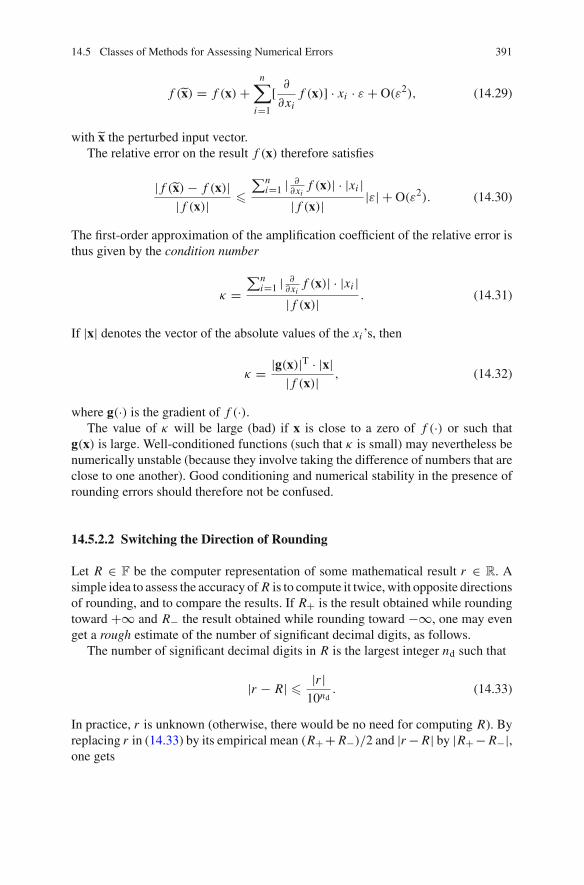
14.5 Classes of Methods for Assessing Numerical Errors 391

f (x) = f (x) +n∑

i=1

[ ρ

ρxif (x)] · xi · α + O(α2), (14.29)

with x the perturbed input vector.The relative error on the result f (x) therefore satisfies

| f (x) − f (x)|| f (x)| �

∑ni=1 | ρ

ρxif (x)| · |xi |

| f (x)| |α| + O(α2). (14.30)

The first-order approximation of the amplification coefficient of the relative error isthus given by the condition number

σ =∑n

i=1 | ρρxi

f (x)| · |xi || f (x)| . (14.31)

If |x| denotes the vector of the absolute values of the xi ’s, then

σ = |g(x)|T · |x|| f (x)| , (14.32)

where g(·) is the gradient of f (·).The value of σ will be large (bad) if x is close to a zero of f (·) or such that

g(x) is large. Well-conditioned functions (such that σ is small) may nevertheless benumerically unstable (because they involve taking the difference of numbers that areclose to one another). Good conditioning and numerical stability in the presence ofrounding errors should therefore not be confused.

14.5.2.2 Switching the Direction of Rounding

Let R ∇ F be the computer representation of some mathematical result r ∇ R. Asimple idea to assess the accuracy of R is to compute it twice, with opposite directionsof rounding, and to compare the results. If R+ is the result obtained while roundingtoward +→ and R− the result obtained while rounding toward −→, one may evenget a rough estimate of the number of significant decimal digits, as follows.

The number of significant decimal digits in R is the largest integer nd such that

|r − R| � |r |10nd

. (14.33)

In practice, r is unknown (otherwise, there would be no need for computing R). Byreplacing r in (14.33) by its empirical mean (R+ + R−)/2 and |r − R| by |R+ − R−|,one gets

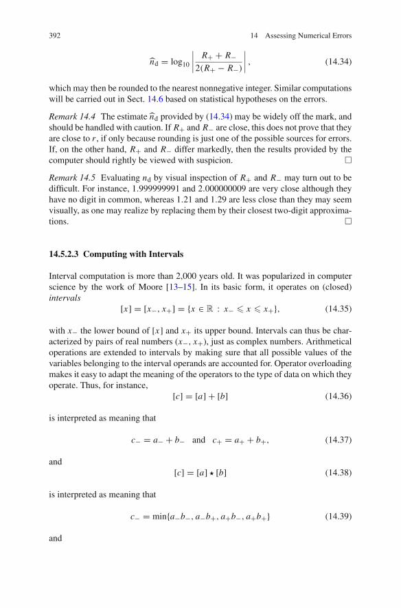
392 14 Assessing Numerical Errors

nd = log10

∣∣∣∣R+ + R−

2(R+ − R−)

∣∣∣∣ , (14.34)

which may then be rounded to the nearest nonnegative integer. Similar computationswill be carried out in Sect. 14.6 based on statistical hypotheses on the errors.

Remark 14.4 The estimate nd provided by (14.34) may be widely off the mark, andshould be handled with caution. If R+ and R− are close, this does not prove that theyare close to r , if only because rounding is just one of the possible sources for errors.If, on the other hand, R+ and R− differ markedly, then the results provided by thecomputer should rightly be viewed with suspicion. �

Remark 14.5 Evaluating nd by visual inspection of R+ and R− may turn out to bedifficult. For instance, 1.999999991 and 2.000000009 are very close although theyhave no digit in common, whereas 1.21 and 1.29 are less close than they may seemvisually, as one may realize by replacing them by their closest two-digit approxima-tions. �

14.5.2.3 Computing with Intervals

Interval computation is more than 2,000 years old. It was popularized in computerscience by the work of Moore [13–15]. In its basic form, it operates on (closed)intervals

[x] = [x−, x+] = {x ∇ R : x− � x � x+}, (14.35)

with x− the lower bound of [x] and x+ its upper bound. Intervals can thus be char-acterized by pairs of real numbers (x−, x+), just as complex numbers. Arithmeticaloperations are extended to intervals by making sure that all possible values of thevariables belonging to the interval operands are accounted for. Operator overloadingmakes it easy to adapt the meaning of the operators to the type of data on which theyoperate. Thus, for instance,

[c] = [a] + [b] (14.36)

is interpreted as meaning that

c− = a− + b− and c+ = a+ + b+, (14.37)

and[c] = [a] � [b] (14.38)

is interpreted as meaning that

c− = min{a−b−, a−b+, a+b−, a+b+} (14.39)

and

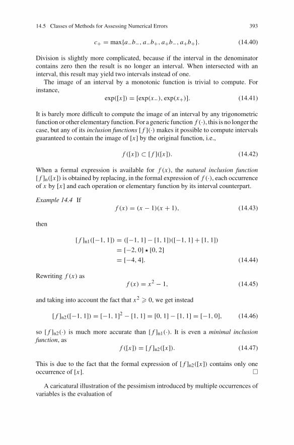
14.5 Classes of Methods for Assessing Numerical Errors 393

c+ = max{a−b−, a−b+, a+b−, a+b+}. (14.40)

Division is slightly more complicated, because if the interval in the denominatorcontains zero then the result is no longer an interval. When intersected with aninterval, this result may yield two intervals instead of one.

The image of an interval by a monotonic function is trivial to compute. Forinstance,

exp([x]) = [exp(x−), exp(x+)]. (14.41)

It is barely more difficult to compute the image of an interval by any trigonometricfunction or other elementary function. For a generic function f (·), this is no longer thecase, but any of its inclusion functions [ f ](·) makes it possible to compute intervalsguaranteed to contain the image of [x] by the original function, i.e.,

f ([x]) ⊂ [ f ]([x]). (14.42)

When a formal expression is available for f (x), the natural inclusion function[ f ]n([x]) is obtained by replacing, in the formal expression of f (·), each occurrenceof x by [x] and each operation or elementary function by its interval counterpart.

Example 14.4 Iff (x) = (x − 1)(x + 1), (14.43)

then

[ f ]n1([−1, 1]) = ([−1, 1] − [1, 1])([−1, 1] + [1, 1])= [−2, 0] � [0, 2]= [−4, 4]. (14.44)

Rewriting f (x) asf (x) = x2 − 1, (14.45)

and taking into account the fact that x2 � 0, we get instead

[ f ]n2([−1, 1]) = [−1, 1]2 − [1, 1] = [0, 1] − [1, 1] = [−1, 0], (14.46)

so [ f ]n2(·) is much more accurate than [ f ]n1(·). It is even a minimal inclusionfunction, as

f ([x]) = [ f ]n2([x]). (14.47)

This is due to the fact that the formal expression of [ f ]n2([x]) contains only oneoccurrence of [x]. �

A caricatural illustration of the pessimism introduced by multiple occurrences ofvariables is the evaluation of

394 14 Assessing Numerical Errors

f (x) = x − x (14.48)

on the interval [−1, 1] using a natural inclusion function. Because the two occur-rences of x in (14.48) are treated as if they were independent,

[ f ]n([−1, 1]) = [−2, 2]. (14.49)

It is thus a good idea to look for formal expressions that minimize the numberof occurrences of the variables. Many other techniques are available to reduce thepessimism of inclusion functions.

Interval computation easily extends to interval vectors and matrices. An intervalvector (or box) [x] is a Cartesian product of intervals, and [f]([x]) is an inclusionfunction for the multivariate vector function f(x) if it computes an interval vector[f]([x]) that contains the image of [x] by f(·), i.e.,

f([x]) ⊂ [f]([x]). (14.50)

In the floating-point implementation of intervals, the real interval [x] is replacedby a machine-representable interval [X ] obtained by outward rounding, i.e., X− isobtained by rounding x− toward −→, and X+ by rounding x+ toward +→. One canthen replace computing on real numbers by computing on machine-representableintervals, thus providing intervals guaranteed to contain the results that would beobtained by computing on real numbers. This conceptually attractive approach isabout as old as computers.

It soon became apparent, however, that its evaluation of the impact of errors couldbe so pessimistic as to become useless. This does not mean that interval analysis can-not be employed, but rather that the problem to be solved must be adequately formu-lated and that specific algorithms must be used. Key ingredients of these algorithmsare

• the elimination of boxes by proving that they contain no solution,• the bisection of boxes over which no conclusion could be reached, in a divide-

and-conquer approach,• and the contraction of boxes that may contain solutions without losing any of these

solutions.

Example 14.5 EliminationAssume that g(x) is the gradient of some cost function to be minimized without

constraint and that [g](·) is an inclusion function for g(·). If

0 /∇ [g]([x]), (14.51)

then (14.50) implies that0 /∇ g([x]). (14.52)

14.5 Classes of Methods for Assessing Numerical Errors 395

The first-order optimality condition (9.6) is thus satisfied nowhere in the box [x],so [x] can be eliminated from further search as it cannot contain any unconstrainedminimizer. �

Example 14.6 BisectionConsider again Example 14.5, but assume now that

0 ∇ [g]([x]), (14.53)

which does not allow [x] to be eliminated. One may then split [x] into [x1] and [x2]and attempt to eliminate these smaller boxes. This is made easier by the fact that inclu-sion functions usually get less pessimistic when the size of their interval argumentsdecreases (until the effect of outward rounding becomes predominant). The curseof dimensionality is of course lurking behind bisection. Contraction, which makesit possible to reduce the size of [x] without losing any solution, is thus particularlyimportant when dealing with high-dimensional problems. �

Example 14.7 ContractionLet f (·) be a scalar univariate function, with a continuous first derivative on [x],

and let x� and x0 be two points in [x], with f (x�) = 0. The mean-value theoremimplies that there exits c ∇ [x] such that

f (c) = f (x�) − f (x0)

x� − x0. (14.54)

In other words,

x� = x0 − f (x0)

f (c). (14.55)

If an inclusion function [ f ](·) is available for f (·), then

x� ∇ x0 − f (x0)

[ f ]([x]) . (14.56)

Now x� also belongs to [x], so

x� ∇ [x] ⊂(

x0 − f (x0)

[ f ]([x]))

, (14.57)

which may be much smaller than [x]. This suggests iterating

[xk+1] = [xk] ⊂(

xk − f (xk)

[ f ]([xk]))

, (14.58)

with xk some point in [xk], for instance its center. Any solution belonging to [xk]belongs also to [xk+1], which may be much smaller.

396 14 Assessing Numerical Errors

The resulting interval Newton method is more complicated than it seems, as theinterval denominator [ f ]([xk]) may contain zero, so [xk+1] may consist of two inter-vals, each of which will have to be processed at the next iteration. The interval Newtonmethod can be extended to finding approximation by boxes of all the solutions ofsystems of nonlinear equations in several unknowns [16]. �

Remark 14.6 Interval computations may similarly be used to get bounds on theremainder of Taylor expansions, thus making it possible to bound method errors.Consider, for instance, the kth order Taylor expansion of a scalar univariate functionf (·) around xc

f (x) = f (xc) +k∑

i=1

1

i ! f (i) (xc) · (x − xc)i + r (x, xc, ν) , (14.59)

where

r (x, xc, ν) = 1

(k + 1)! f (k+1)(ν) · (x − xc)k+1 (14.60)

is the Taylor remainder. Equation (14.59) holds true for some unknown ν in [x, xc].An inclusion function [ f ](·) for f (·) is thus

[ f ]([x]) = f (xc) +k∑

i=1

1

i ! f (i) (xc) · ([x] − xc)i + [r ] ([x], xc, [x]) , (14.61)

with [r ](·, ·, ·) an inclusion function for r(·, ·, ·) and xc any point in [x], for instanceits center. �

With the help of these concepts, approximate but guaranteed solutions can befound to problems such as

• finding all the solutions of a system of nonlinear equations [16],• characterizing a set defined by nonlinear inequalities [17],• finding all the global minimizers of a non-convex cost function [18, 19],• solving a Cauchy problem for a nonlinear ODE for which no closed-form solution

is known [20–22].

Applications to engineering are presented in [17].Interval analysis assumes that the error committed at each step of the computation

may be as damaging as it can get. Fortunately, the situation is usually not that bad,as some errors partly compensate others. This motivates replacing such a worst-caseanalysis by a probabilistic analysis of the results obtained when the same computa-tions are carried out several times with different realizations of the rounding errors,as in Sect. 14.6.

14.5 Classes of Methods for Assessing Numerical Errors 397

14.5.2.4 Running Error Analysis

Running error analysis [4, 23, 24] propagates an evaluation of the effect of roundingerrors alongside the floating-point computations. Let αx be a bound on the absoluteerror on x , such that

|X − x | � αx . (14.62)

When rounding is toward the closest double, as usual, approximate bounds on theresults of arithmetic operations are computed as follows:

z = x + y ∞ αz = u|fl(X + Y )| + αx + αy, (14.63)

z = x − y ∞ αz = u|fl(X − Y )| + αx + αy, (14.64)

z = x � y ∞ αz = u|fl(X � Y )| + αx |Y | + αy |X |, (14.65)

z = x/y ∞ αz = u|fl(X/Y )| + αx |Y | + αy |X |Y 2 . (14.66)

The first term on the right-hand side of (14.63)–(14.66) is deduced from (14.14).The following terms propagate input errors to the output while neglecting productsof error terms. The method is much simpler to implement than the interval approachof Sect. 14.5.2.3, but the resulting bounds on the effect of rounding errors are approx-imate and method errors are not taken into account.

14.5.2.5 Randomly Perturbing Computation

This method finds its origin in the work of La Porte and Vignes [1, 25–28]. Itwas initially known under the French acronym CESTAC (for Contrôle et Estima-tion STochastique des Arrondis de Calcul) and is now implemented in the soft-ware CADNA (for Control of Accuracy and Debugging for Numerical Applications),freely available at http://www-pequan.lip6.fr/cadna/. CESTAC/CADNA, describedin more detail in the following section, may be viewed as a Monte Carlo method.The same computation is performed several times while picking the rounding errorat random, and statistical characteristics of the population of results thus obtainedare evaluated. If the results provided by the computer vary widely because of suchtiny perturbations, this is a clear indication of their lack of credibility. More quanti-tatively, these results will be provided with estimates of their numbers of significantdecimal digits.

14.6 CESTAC/CADNA

The presentation of the method is followed by a discussion of its validity conditions,which can partly be checked by the method itself.

398 14 Assessing Numerical Errors

14.6.1 Method

Let r ∇ R be some real quantity to be evaluated by a program and Ri ∇ F bethe corresponding floating-point result, as provided by the i th run of this program(i = 1, . . . , N ). During each run, the result of each operation is randomly roundedeither toward +→ or toward −→, with the same probability. Each Ri may thusbe seen as an approximation of r . The fundamental hypothesis on which CES-TAC/CADNA is based is that these Ri ’s are independently and identically distributedaccording to a Gaussian law, with mean r .

Let μ be the arithmetic mean of the results provided by the computer in N runs

μ = 1

N

N∑

i=1

Ri . (14.67)

Since N is finite, μ is not equal to r , but it is in general closer to r than any of theRi ’s (μ is the maximum-likelihood estimate of r under the fundamental hypothesis).Let β be the empirical standard deviation of the Ri ’s

β =√√√√ 1

N − 1

N∑

i=1

(Ri − μ)2, (14.68)

which characterizes the dispersion of the Ri ’s around their mean. Student’s t testmakes it possible to compute an interval centered at μ and having a given probabilityκ of containing r

Prob

[|μ − r | � τβ≈

N

]= κ. (14.69)

In (14.69), the value of τ depends on the value of κ (to be chosen by the user) andon the number of degrees of freedom, which is equal to N − 1 since there are N datapoints Ri linked to μ by the equality constraint (14.67). Typical values are κ = 0.95,which amounts to accepting to be wrong in 5% of the cases, and N = 2 or 3, to keepthe volume of computation manageable. From (14.33), the number nd of significantdecimal digits in μ satisfies

10nd � |r ||μ − r | . (14.70)

Replace |μ − r | by τβ/≈

N and r by μ to get an estimate of nd as the nonnegativeinteger that is the closest to

nd = log10|μ|τβ≈

N

= log10|μ|β

− log10τ≈N

. (14.71)

For κ = 0.95,

14.6 CESTAC/CADNA 399

nd ∈ log10|μ|β

− 0.953 if N = 2, (14.72)

and

nd ∈ log10|μ|β

− 0.395 if N = 3. (14.73)

Remark 14.7 Assume N = 2 and denote the results of the two runs by R+ and R−.Then

log10|μ|β

= log10|R+ + R−||R+ − R−| − log10

≈2, (14.74)

so

nd ∈ log10|R+ + R−||R+ − R−| − 1.1. (14.75)

Compare with (14.34), which is such that

nd ∈ log10|R+ + R−||R+ − R−| − 0.3. (14.76)

�

Based on this analysis, one may now present each result in a format that onlyshows the decimal digits that are deemed significant. A particularly spectacular caseis when the estimated number of significant digits becomes zero (nd < 0.5), whichamounts to saying that nothing is known of the result, not even its sign. This led tothe concept of computational zero (CZ): the result of a numerical computation is aCZ if its value is zero or if it contains no significant digit. A very large floating-pointnumber may turn out to be a CZ while another with a very small magnitude may notbe a CZ.

The application of this approach depends on the type of algorithm beingconsidered, as defined in Sect. 14.2.

For exact finite algorithms, CESTAC/CADNA can provide each result with anestimate of its number of significant decimal digits. When the algorithm involvesconditional branching, one should be cautious about the CESTAC/CADNA assess-ment of the accuracy of the results, as the perturbed runs may not all follow the samebranch of the code, which would make the hypothesis of a Gaussian distribution ofthe results particularly questionable. This suggests analysing not only the precisionof the end results but also that of all floating-point intermediary results (at least thoseinvolved in conditions). This may be achieved by running two or three executionsof the algorithm in parallel. Operator overloading makes it possible to avoid hav-ing to modify heavily the code to be tested. One just has to declare the variablesto be monitored as stochastic. For more details, see http://www-anp.lip6.fr/english/cadna/. As soon as a CZ is detected, the results of all subsequent computations shouldbe subjected to serious scrutiny. One may even decide to stop computation there and

400 14 Assessing Numerical Errors

look for an alternative formulation of the problem, thus using CESTAC/CADNA asa numerical debugger.

For exact iterative algorithms, CESTAC/CADNA also provides rational stoppingrules. Many such algorithms are verifiable (at least partly) and should mathematicallybe stopped when some (possibly vector) quantity takes the value zero. When lookingfor a root of the system of nonlinear equations f(x) = 0, for instance, this quantitymight be f(xk). When looking for some unconstrained minimizer of a differentiablecost function, it might be g(xk), with g(·) the gradient function of this cost function.One may thus decide to stop when the floating-point representations of all the entriesof f(xk) or g(xk) have become CZs, i.e., are either zero or no longer contain significantdecimal digits. This amounts to saying that it has become impossible to prove that thesolution has not been reached given the precision with which computation has beencarried out. The delicate choice of threshold parameters in the stopping tests is thenbypassed. The price to be paid to assess the precision of the results is a multiplicationby two or three of the volume of computation. This seems all the more reasonablethat iterative algorithms often turn out to be stopped much earlier than with moretraditional stopping rules, so the total volume of computation may even decrease.When the algorithm is not verifiable, it may still be possible to define a rationalstopping rule. If, for instance, one wants to compute

S = limn→→ Sn =

n∑

i=1

fi , (14.77)

then one may stop when|Sn − Sn−1| = CZ, (14.78)

which means the iterative increment is no longer significant. (The usual transcenden-tal functions are not computed via such an evaluation of series, and the proceduresactually used are quite sophisticated [29].)

For approximate algorithms, one should minimize the global error resulting fromthe combination of the method and rounding errors. CESTAC/CADNA may helpfinding a good tradeoff by contributing to the assessment of the effects of the latter,provided that the effects of the former are assessed by some other method.

14.6.2 Validity Conditions

A detailed study of the conditions under which this approach provides reliable resultsis presented in [6, 8]; see also [1]. Key ingredients are (14.25), which results from afirst-order forward error analysis, and the central-limit theorem. In its simplest form,this theorem states that the averaged sum of n independent random variables xi

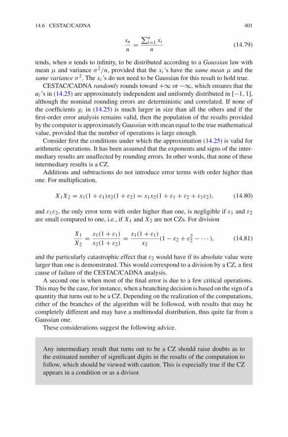
14.6 CESTAC/CADNA 401

sn

n=

∑ni=1 xi

n(14.79)

tends, when n tends to infinity, to be distributed according to a Gaussian law withmean μ and variance β 2/n, provided that the xi ’s have the same mean μ and thesame variance β 2. The xi ’s do not need to be Gaussian for this result to hold true.

CESTAC/CADNA randomly rounds toward +→ or −→, which ensures that theδi ’s in (14.25) are approximately independent and uniformly distributed in [−1, 1],although the nominal rounding errors are deterministic and correlated. If none ofthe coefficients gi in (14.25) is much larger in size than all the others and if thefirst-order error analysis remains valid, then the population of the results providedby the computer is approximately Gaussian with mean equal to the true mathematicalvalue, provided that the number of operations is large enough.

Consider first the conditions under which the approximation (14.25) is valid forarithmetic operations. It has been assumed that the exponents and signs of the inter-mediary results are unaffected by rounding errors. In other words, that none of theseintermediary results is a CZ.

Additions and subtractions do not introduce error terms with order higher thanone. For multiplication,

X1 X2 = x1(1 + α1)x2(1 + α2) = x1x2(1 + α1 + α2 + α1α2), (14.80)

and α1α2, the only error term with order higher than one, is negligible if α1 and α2are small compared to one, i.e., if X1 and X2 are not CZs. For division

X1

X2= x1(1 + α1)

x2(1 + α2)= x1(1 + α1)

x2(1 − α2 + α2

2 − · · · ), (14.81)

and the particularly catastrophic effect that α2 would have if its absolute value werelarger than one is demonstrated. This would correspond to a division by a CZ, a firstcause of failure of the CESTAC/CADNA analysis.

A second one is when most of the final error is due to a few critical operations.This may be the case, for instance, when a branching decision is based on the sign of aquantity that turns out to be a CZ. Depending on the realization of the computations,either of the branches of the algorithm will be followed, with results that may becompletely different and may have a multimodal distribution, thus quite far from aGaussian one.

These considerations suggest the following advice.

Any intermediary result that turns out to be a CZ should raise doubts as tothe estimated number of significant digits in the results of the computation tofollow, which should be viewed with caution. This is especially true if the CZappears in a condition or as a divisor.

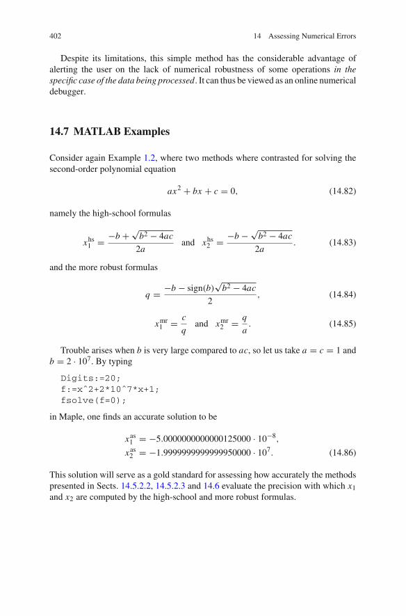
402 14 Assessing Numerical Errors

Despite its limitations, this simple method has the considerable advantage ofalerting the user on the lack of numerical robustness of some operations in thespecific case of the data being processed. It can thus be viewed as an online numericaldebugger.

14.7 MATLAB Examples

Consider again Example 1.2, where two methods where contrasted for solving thesecond-order polynomial equation

ax2 + bx + c = 0, (14.82)

namely the high-school formulas

xhs1 = −b + ≈

b2 − 4ac

2aand xhs

2 = −b − ≈b2 − 4ac

2a. (14.83)

and the more robust formulas

q = −b − sign(b)≈

b2 − 4ac

2, (14.84)

xmr1 = c

qand xmr

2 = q

a. (14.85)

Trouble arises when b is very large compared to ac, so let us take a = c = 1 andb = 2 · 107. By typing

Digits:=20;f:=xˆ2+2*10ˆ7*x+1;fsolve(f=0);

in Maple, one finds an accurate solution to be

xas1 = −5.0000000000000125000 · 10−8,

xas2 = −1.9999999999999950000 · 107. (14.86)

This solution will serve as a gold standard for assessing how accurately the methodspresented in Sects. 14.5.2.2, 14.5.2.3 and 14.6 evaluate the precision with which x1and x2 are computed by the high-school and more robust formulas.

14.7 MATLAB Examples 403

14.7.1 Switching the Direction of Rounding

Implementing the switching method presented in Sect. 14.5.2.2, requirescontrolling rounding modes. Unfortunately, MATLAB does not allow one to dothis directly, but it is possible via the INTLAB toolbox [30]. Once this toolbox hasbeen installed and started by the MATLAB command startintlab, the commandsetround(-1) switches the rounding mode to toward −→, while the commandsetround(1) switches it to toward +→ and setround(0) restores it to towardthe nearest. Note that MATLAB’s sqrt, which is not IEEE-754 compliant, must bereplaced by INTLAB’s sqrt_rnd for the computation of square roots needed inthe example.

When rounding toward minus infinity, the results are

xhs−1 = −5.029141902923584 · 10−8,

xhs−2 = −1.999999999999995 · 107,

xmr−1 = −5.000000000000013 · 10−8,

xmr−2 = −1.999999999999995 · 107. (14.87)

When rounding toward plus infinity, they become

xhs+1 = −4.842877388000488 · 10−8,

xhs+2 = −1.999999999999995 · 107,

xmr+1 = −5.000000000000012 · 10−8,

xmr+2 = −1.999999999999995 · 107. (14.88)

Applying (14.34), we then get

nd(xhs1 ) ∈ 1.42,

nd(xhs2 ) ∈ 15.72,

nd(xmr1 ) ∈ 15.57,

nd(xmr2 ) ∈ 15.72. (14.89)

Rounding these estimates to the closest nonnegative integer, we can write only thedecimal digits that are deemed significant in the results. Thus

xhs1 = −5 · 10−8,

xhs2 = −1.999999999999995 · 107,

xmr1 = −5.000000000000013 · 10−8,

xmr2 = −1.999999999999995 · 107. (14.90)

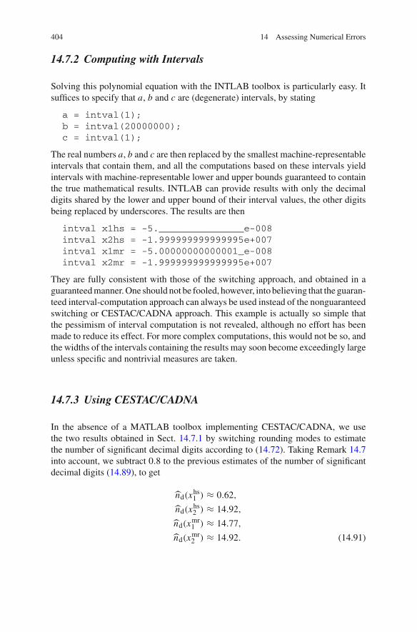
404 14 Assessing Numerical Errors

14.7.2 Computing with Intervals

Solving this polynomial equation with the INTLAB toolbox is particularly easy. Itsuffices to specify that a, b and c are (degenerate) intervals, by stating

a = intval(1);b = intval(20000000);c = intval(1);

The real numbers a, b and c are then replaced by the smallest machine-representableintervals that contain them, and all the computations based on these intervals yieldintervals with machine-representable lower and upper bounds guaranteed to containthe true mathematical results. INTLAB can provide results with only the decimaldigits shared by the lower and upper bound of their interval values, the other digitsbeing replaced by underscores. The results are then

intval x1hs = -5._______________e-008intval x2hs = -1.999999999999995e+007intval x1mr = -5.00000000000001_e-008intval x2mr = -1.999999999999995e+007

They are fully consistent with those of the switching approach, and obtained in aguaranteed manner. One should not be fooled, however, into believing that the guaran-teed interval-computation approach can always be used instead of the nonguaranteedswitching or CESTAC/CADNA approach. This example is actually so simple thatthe pessimism of interval computation is not revealed, although no effort has beenmade to reduce its effect. For more complex computations, this would not be so, andthe widths of the intervals containing the results may soon become exceedingly largeunless specific and nontrivial measures are taken.

14.7.3 Using CESTAC/CADNA

In the absence of a MATLAB toolbox implementing CESTAC/CADNA, we usethe two results obtained in Sect. 14.7.1 by switching rounding modes to estimatethe number of significant decimal digits according to (14.72). Taking Remark 14.7into account, we subtract 0.8 to the previous estimates of the number of significantdecimal digits (14.89), to get

nd(xhs1 ) ∈ 0.62,

nd(xhs2 ) ∈ 14.92,

nd(xmr1 ) ∈ 14.77,

nd(xmr2 ) ∈ 14.92. (14.91)

14.7 MATLAB Examples 405

Rounding these estimates to the closest nonnegative integer, and keeping only thedecimal digits that are deemed significant, we get the slightly modified results

xhs1 = −5 · 10−8,

xhs2 = −1.99999999999999 · 107,

xmr1 = −5.00000000000001 · 10−8,

xmr2 = −1.99999999999999 · 107. (14.92)

The CESTAC/CADNA approach thus suggests discarding digits that the switchingapproach deemed valid. On this specific example, the gold standard (14.86) revealsthat the more optimistic switching approach is right, as these digits are indeed correct.Both approaches, as well as interval computations, clearly evidence a problem withx1 as computed with the high-school method.

14.8 In Summary

• Moving from analytic calculus to numerical computation with floating-point num-bers translates into unavoidable rounding errors, the consequences of which mustbe analyzed and minimized.

• Potentially the most dangerous operations are subtracting numbers that are closeto one another, dividing by a CZ, and branching based on the value or sign of aCZ.

• Among the methods available in the literature to assess the effect of roundingerrors, those using the computer to evaluate the consequences of its own errorshave two advantages: they are applicable to broad classes of algorithms, and theytake the specifics of the data being processed into account.

• A mere switching of the direction of rounding may suffice to reveal a large uncer-tainty in numerical results.

• Interval analysis produces guaranteed results with error estimates that may be verypessimistic unless dedicated algorithms are used. This limits its applicability, butbeing able to provide bounds on method errors is a considerable advantage.

• Running error analysis loses this advantage and only provides approximate boundson the effect of the propagation of rounding errors, but is much simpler to imple-ment in an ad hoc manner.

• The random-perturbation approach CESTAC/CADNA does not suffer from thepessimism of interval analysis. It should nevertheless be used with caution as avariant of casting out the nines, which cannot guarantee that the numerical resultsprovided by the computer are correct but may detect that they are not. It cancontribute to checking whether its conditions of validity are satisfied.

406 14 Assessing Numerical Errors

References

1. Pichat, M., Vignes, J.: Ingénierie du contrôle de la précision des calculs sur ordinateur. EditionsTechnip, Paris (1993)

2. Goldberg, D.: What every computer scientist should know about floating-point arithmetic.ACM Comput. Surv. 23(1), 5–48 (1991)

3. IEEE: IEEE standard for floating-point arithmetic. Technical Report IEEE Standard 754–2008, IEEE Computer Society (2008)

4. Higham, N.: Accuracy and Stability of Numerical Algorithms, 2nd edn. SIAM, Philadelphia(2002)

5. Muller, J.M., Brisebarre, N., de Dinechin, F., Jeannerod, C.P., Lefèvre, V., Melquiond, G.,Revol, N., Stehlé, D., Torres, S.: Handbook of Floating-Point Arithmetic. Birkhäuser, Boston(2010)

6. Chesneaux, J.M.: Etude théorique et implémentation en ADA de la méthode CESTAC. Ph.D.thesis, Université Pierre et Marie Curie (1988)

7. Chesneaux, J.M.: Study of the computing accuracy by using probabilistic approach. In: Ull-rich, C. (ed.) Contribution to Computer Arithmetic and Self-Validating Methods, pp. 19–30.J.C. Baltzer AG, Amsterdam (1990)

8. Chesneaux, J.M.: L’arithmétique stochastique et le logiciel CADNA. Université Pierre etMarie Curie, Habilitation à diriger des recherches (1995)

9. Kulisch, U.: Very fast and exact accumulation of products. Computing 91, 397–405 (2011)10. Wilkinson, J.: Rounding Errors in Algebraic Processes, reprinted edn. Dover, New York (1994)11. Wilkinson, J.: Modern error analysis. SIAM Rev. 13(4), 548–568 (1971)12. Kahan, W.: How futile are mindless assessments of roundoff in floating-point computation?

www.cs.berkeley.edu/~wkahan/Mindless.pdf (2006) (work in progress)13. Moore, R.: Automatic error analysis in digital computation. Technical Report LMSD-48421,

Lockheed Missiles and Space Co, Palo Alto, CA (1959)14. Moore, R.: Interval Analysis. Prentice-Hall, Englewood Cliffs (1966)15. Moore, R.: Methods and Applications of Interval Analysis. SIAM, Philadelphia (1979)16. Neumaier, A.: Interval Methods for Systems of Equations. Cambridge University Press, Cam-

bridge (1990)17. Jaulin, L., Kieffer, M., Didrit, O., Walter, E.: Applied Interval Analysis. Springer, London

(2001)18. Ratschek, H., Rokne, J.: New Computer Methods for Global Optimization. Ellis Horwood,

Chichester (1988)19. Hansen, E.: Global Optimization Using Interval Analysis. Marcel Dekker, New York (1992)20. Bertz, M., Makino, K.: Verified integration of ODEs and flows using differential algebraic

methods on high-order Taylor models. Reliab. Comput. 4, 361–369 (1998)21. Nedialkov, N., Jackson, K., Corliss, G.: Validated solutions of initial value problems for

ordinary differential equations. Appl. Math. Comput. 105(1), 21–68 (1999)22. Nedialkov, N.: VNODE-LP, a validated solver for initial value problems in ordinary differ-

ential equations. Technical Report CAS-06-06-NN, Department of Computing and Software,McMaster University, Hamilton (2006)

23. Wilkinson, J.: Error analysis revisited. IMA Bull. 22(11/12), 192–200 (1986)24. Zahradnicky, T., Lorencz, R.: FPU-supported running error analysis. Acta Polytechnica 50(2),

30–36 (2010)25. La Porte, M., Vignes, J.: Algorithmes numériques, analyse et mise en œuvre, 1: Arithmétique

des ordinateurs. Systèmes linéaires. Technip, Paris (1974)26. Vignes, J.: New methods for evaluating the validity of the results of mathematical computa-

tions. Math. Comput. Simul. 20(4), 227–249 (1978)27. Vignes, J., Alt, R., Pichat, M.: Algorithmes numériques, analyse et mise en œuvre, 2: équations

et systèmes non linéaires. Technip, Paris (1980)28. Vignes, J.: A stochastic arithmetic for reliable scientific computation. Math. Comput. Simul.

35, 233–261 (1993)

References 407

29. Muller, J.M.: Elementary Functions, Algorithms and Implementation, 2nd edn. Birkhäuser,Boston (2006)

30. Rump, S.: INTLAB - INTerval LABoratory. In: Csendes, T. (ed.) Developments in ReliableComputing, pp. 77–104. Kluwer Academic Publishers, Dordrecht (1999)

Chapter 15WEB Resources to Go Further

This chapter suggests web sites that give access to numerical software as well asto additional information on concepts and methods presented in the other chapters.Most of the resources described can be used at no cost. Classification is not tight, asthe same URL may point to various types of facilities.

15.1 Search Engines

Among their countless applications, general-purpose search engines can be usedto find the home pages of important contributors to numerical analysis. It is notuncommon for downloadable lecture slides, electronic versions of papers, or evenbooks to be freely on offer via these pages.

Google Scholar (http://scholar.google.com/) is a more specialized search engineaimed at the academic literature. It can be used to find who quoted a specific authoror paper, thereby making it possible to see what has been the fate of an interestingidea. By creating a public scholar profile, one may even get suggestions of potentiallyinteresting papers.

Publish or Perish (http://www.harzing.com/) retrieves and analyzes academiccitations based on Google Scholar. It can be used to assess the impact of a method,an author, or a journal in the scientific community.

YouTube (http://www.youtube.com) gives access to many pedagogical videos ontopics covered by this book.

15.2 Encyclopedias

For just about any concept or numerical method mentioned in this book, additionalinformation may be found in Wikipedia (http://en.wikipedia.org/), which now con-tains more than four million articles.

É. Walter, Numerical Methods and Optimization, 409DOI: 10.1007/978-3-319-07671-3_15,© Springer International Publishing Switzerland 2014

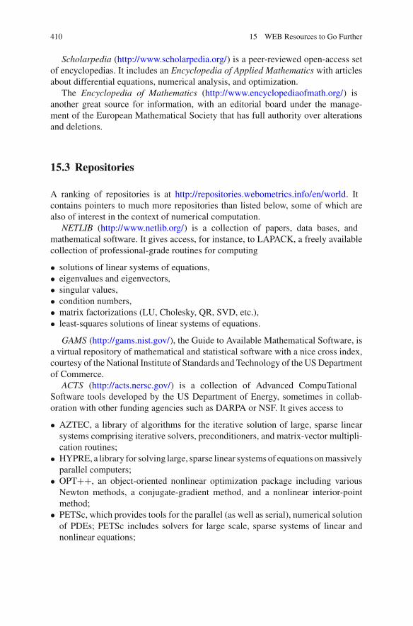
410 15 WEB Resources to Go Further

Scholarpedia (http://www.scholarpedia.org/) is a peer-reviewed open-access setof encyclopedias. It includes an Encyclopedia of Applied Mathematics with articlesabout differential equations, numerical analysis, and optimization.

The Encyclopedia of Mathematics (http://www.encyclopediaofmath.org/) isanother great source for information, with an editorial board under the manage-ment of the European Mathematical Society that has full authority over alterationsand deletions.

15.3 Repositories

A ranking of repositories is at http://repositories.webometrics.info/en/world. Itcontains pointers to much more repositories than listed below, some of which arealso of interest in the context of numerical computation.

NETLIB (http://www.netlib.org/) is a collection of papers, data bases, andmathematical software. It gives access, for instance, to LAPACK, a freely availablecollection of professional-grade routines for computing

• solutions of linear systems of equations,• eigenvalues and eigenvectors,• singular values,• condition numbers,• matrix factorizations (LU, Cholesky, QR, SVD, etc.),• least-squares solutions of linear systems of equations.

GAMS (http://gams.nist.gov/), the Guide to Available Mathematical Software, isa virtual repository of mathematical and statistical software with a nice cross index,courtesy of the National Institute of Standards and Technology of the US Departmentof Commerce.

ACTS (http://acts.nersc.gov/) is a collection of Advanced CompuTationalSoftware tools developed by the US Department of Energy, sometimes in collab-oration with other funding agencies such as DARPA or NSF. It gives access to

• AZTEC, a library of algorithms for the iterative solution of large, sparse linearsystems comprising iterative solvers, preconditioners, and matrix-vector multipli-cation routines;

• HYPRE, a library for solving large, sparse linear systems of equations on massivelyparallel computers;

• OPT++, an object-oriented nonlinear optimization package including variousNewton methods, a conjugate-gradient method, and a nonlinear interior-pointmethod;

• PETSc, which provides tools for the parallel (as well as serial), numerical solutionof PDEs; PETSc includes solvers for large scale, sparse systems of linear andnonlinear equations;

15.3 Repositories 411

• ScaLAPACK, a library of high-performance linear algebra routines for distributed-memory computers and networks of workstations; ScaLAPACK is a continuationof the LAPACK project;

• SLEPc, a package for the solution of large, sparse eigenproblems on parallel com-puters, as well as related problems such as singular value decomposition;

• SUNDIALS [1], a family of closely related solvers: CVODE, for systems of ordi-nary differential equations, CVODES, a variant of CVODE for sensitivity analysis,KINSOL, for systems of nonlinear algebraic equations, and IDA, for systems ofdifferential-algebraic equations; these solvers can deal with extremely large sys-tems, in serial or parallel environments;

• SuperLU, a general purpose library for the direct solution of large, sparse, non-symmetric systems of linear equations via LU factorization;

• TAO, a large-scale optimization software, including nonlinear least squares, uncon-strained minimization, bound-constrained optimization, and general nonlinearoptimization, with strong emphasis on the reuse of external tools where appro-priate; TAO can be used in serial or parallel environments.

Pointers to a number of other interesting packages are also provided in the pagesdedicated to each of these products.

CiteSeerX (http://citeseerx.ist.psu.edu) focuses primarily on the literature incomputer and information science. It can be used to find papers that quote someother papers of interest and often provide a free access to electronic versions of thesepapers.

The Collection of Computer Science Bibliographies hosts more than three millionreferences, mostly to journal articles, conference papers, and technical reports. Aboutone million of them contains a URL for an online version of the paper (http://liinwww.ira.uka.de/bibliography).

The Arxiv Computing Research Repository (http://arxiv.org/) allows researchersto search for and download papers through its online repository, at no charge.

HAL (http://hal.archives-ouvertes.fr/) is another multidisciplinary open accessarchive for the deposit and dissemination of scientific research papers and PhDdissertations.

Interval Computation (http://www.cs.utep.edu/interval-comp/) is a rich source ofinformation about guaranteed computation based on interval analysis.

15.4 Software

15.4.1 High-Level Interpreted Languages

High-level interpreted languages are mainly used for prototyping and teaching, aswell as for designing convenient interfaces with compiled code offering faster exe-cution.

412 15 WEB Resources to Go Further

MATLAB (http://www.mathworks.com/products/matlab/) is the main reference inthis context. Interesting material on numerical computing with MATLAB by CleveMoler, chairman and chief scientist at The MathWorks, can be downloaded at http://www.mathworks.com/moler/.

Despite being deservedly popular, MATLAB has several drawbacks:

• it is expensive (especially for industrial users who do not benefit of educationalprices),

• the MATLAB source code developed cannot be used by others (unless they alsohave access to MATLAB),

• parts of the source code cannot be accessed.

For these reasons, or if one does not feel comfortable with a single provider, the twofollowing alternatives are worth considering:

GNU Octave (http://www.gnu.org/software/octave/) was built with MATLABcompatibility in mind; it gives free access to all of its source code and is freelyredistributable under the terms of the GNU General Public License (GPL); (GNU isthe recursive acronym of GNU is Not Unix, a private joke for specialists of operatingsystems;)

Scilab (http://www.scilab.org/en), initially developed by Inria, also gives accessto all of its source code. It is distributed under the CeCILL license (GPL compatible).

While some of the MATLAB toolboxes are commercial products, others arefreely available, at least for a nonprofit use. An interesting case in point was INT-LAB (http://www.ti3.tu-harburg.de/rump/intlab/) a toolbox for guaranteed numeri-cal computation based on interval analysis that features, among many other things,automatic differentiation, and rounding-mode control. INTLAB is now availablefor a nominal fee. Chebfun, an open-source software system that can be used,among many other things, for high-precision high-order polynomial interpolationbased on the use of the barycentric Lagrange formula and Chebyshev points, canbe obtained at http://www2.maths.ox.ac.uk/chebfun/. Free toolboxes implement-ing Kriging are DACE (for Design and Analysis of Computer Experiments, http://www2.imm.dtu.dk/~hbn/dace/) and STK (for Small Toolbox for Kriging, http://sourceforge.net/projects/kriging/). SuperEGO, a MATLAB package for constrainedoptimization based on Kriging, can be obtained (for academic use only) by request toP.Y. Papalambros by email at pyp@umich.edu. Other free resources can be obtainedat http://www.mathworks.com/matlabcentral/fileexchange/.

Another language deserving mention is R (http://www.r-project.org/), mainlyused by statisticians but not limited to statistics. R is another GNU project. Pointersto R packages for Kriging and efficient global optimization (EGO) are available athttp://ls11-www.cs.uni-dortmund.de/rudolph/kriging/dicerpackage.

Many resources for scientific computing in Python (including SciPy) are listed at(http://www.scipy.org/Topical_Software). The Python implementation is under anopen source license that makes it freely usable and distributable, even for commer-cial use.

15.4 Software 413

15.4.2 Libraries for Compiled Languages

GSL is the GNU Scientific Library (http://www.gnu.org/software/gsl/), for C andC++ programmers. Free software under the GNU GPL, GSL provides over 1,000functions with a detailed documentation [2], an updated version of which can bedownloaded freely. An extensive test suite is also provided. Most of the main topicsof this book are covered.

Numerical Recipes (http://www.nr.com/) releases the code presented in theeponymous books at a modest cost, but with a license that does not allow redis-tribution.

Classical commercial products are IMSL and NAG.

15.4.3 Other Resources for Scientific Computing

The NEOS server (http://www.neos-server.org/neos/) can be used to solve possiblylarge-scale optimization problems without having to buy and manage the requiredsoftware. The users may thus concentrate on the definition of their optimizationproblems. NEOS stands for network-enabled optimization software. Information onoptimization is also provided at http://neos-guide.org.

BARON (http://archimedes.cheme.cmu.edu/baron/baron.html) is a system forsolving nonconvex optimization problems. Although commercial versions are avail-able, it can also be accessed freely via the NEOS server.

FreeFEM++ (http://www.freefem.org/) is a finite-element solver for PDEs. Ithas already been used on problems with more than 109 unknowns.

FADBAD++ (http://www.fadbad.com/fadbad.html) implements automaticdifferentiation in forward and backward modes using templates and operator over-loading in C++.

VNODE, for Validated Numerical ODE, is a C++package for computing rigorousbounds on the solutions of initial-value problems for ODEs. It is available at http://www.cas.mcmaster.ca/~nedialk/Software/VNODE/VNODE.shtml.

COMSOL Multiphysics (http://www.comsol.com/) is a commercial finite-elementenvironment for the simulation of PDE models with complicated boundary condi-tions. Problems involving, for instance, chemistry and heat transfer and fluid mechan-ics can be handled.

15.5 OpenCourseWare

OpenCourseWare, or OCW, consists of course material created by universities andshared freely via the Internet. Material may include videos, lecture notes, slides,exams and solutions, etc. Among the institutions offering courses in applied mathe-matics and computer science are

414 15 WEB Resources to Go Further

• the MIT (http://ocw.mit.edu/),• Harvard (http://www.extension.harvard.edu/open-learning-initiative),• Stanford (http://see.stanford.edu/), with, for instance, two series of lectures about

linear systems and convex optimization by Stephen Boyd,• Berkeley (http://webcast.berkeley.edu/),• the University of South Florida (http://mathforcollege.com/nm/).

The OCW finder (http://www.opencontent.org/ocwfinder/) can be used to searchfor courses across universities. Also of interest is Wolfram’s Demonstrations Project(http://demonstrations.wolfram.com/), with topics about computation and numericalanalysis.

Massive Open Online Courses, or MOOCs, are made available in real time viathe Internet to potentially thousands of students, with various levels of interactivity.MOOC providers include edX, Coursera, and Udacity.

References

1. Hindmarsh, A., Brown, P., Grant, K., Lee, S., Serban, R., Shumaker, D., Woodward, C.:SUNDIALS: suite of nonlinear and differential/algebraic equation solvers. ACM Trans. Math.Softw. 31(3), 363–396 (2005)

2. Galassi et al.: M.: GNU Scientific Library Reference Manual, 3rd edn. Network Theory Ltd,Bristol (2009)

Chapter 16Problems

This chapter consists of problems given over the last 10 years to students as partof their final exam. Some of these problems present theoretically interesting andpractically useful numerical techniques not covered in the previous chapters. Manyof them translate easily into computer-lab work. Most of them build on materialpertaining to several chapters, and this is why they have been collected here.

16.1 Ranking Web Pages

The goal of this problem is to study a simplified version of the famous PageRankalgorithm, used by Google for choosing in which order the pages of potential interestshould be presented when answering a query [1]. Let N be the total number of pagesindexed by Google. (In 2012, N was around a staggering 5 · 1010.) After indexingthese pages from 1 to N , an (N × N ) matrice M is created, such that mi, j is equal toone if there exists a hyperlink in page j pointing toward page i and to zero otherwise(Given the size of M, it is fortunate that it is very sparse...). Denote by xk an N -dimensional vector whose i th entry contains the probability of being in page i after kpage changes if all the pages initially had the same probability, i.e., if x0 was suchthat

x0i = 1

N, i = 1, . . . , N . (16.1)

1. To compute xk , one needs a probabilistic model of the behavior of the WEB surfer.The simplest possible model is to assume that the surfer always moves from onepage to the next by clicking on a button and that all the buttons of a given pagehave the same probability of being selected. One thus obtains the equation of ahuge Markov chain

xk+1 = Sxk, (16.2)

É. Walter, Numerical Methods and Optimization, 415DOI: 10.1007/978-3-319-07671-3_16,© Springer International Publishing Switzerland 2014

416 16 Problems

where S has the same dimensions as M. Explain how S is deduced from M. Whatare the constraints that S must satisfy to express that (i) if one is in any given pagethen one must leave it and (i i) all the ways of doing so have the same probability?What are the constraints satisfied by the entries of xk+1?

2. Assume, for the time being, that each page can be reached from any other pageafter a finite (although potentially very large) number of clicks (this is HypothesisH1). The Markov chain then converges toward a unique stationary state x√, suchthat

x√ = Sx√, (16.3)

and the i th entry of x√ is the probability that the surfer is in page i . The higher thisprobability is the more this page is visible from the others. PageRank basicallyorders the pages answering a given query by decreasing values of the correspond-ing entries of x√. If H1 is satisfied, the eigenvalue of S with the largest modulusis unique, and equal to 1. Deduce from this fact an algorithm to evaluate x√.Assuming that ten pages point in average toward a given page, show that thenumber of arithmetical operations needed to compute xk+1 from xk is O(N ).

3. Unfortunately, H1 is not realistic. Some pages, for instance, do not point towardany other page, which translates into columns of zeros in M. Even when there arebuttons on which to click, the surfer may decide to jump to a page toward whichthe present page does not point. This is why S is replaced in (16.2) by

A = (1 − ∂)S + ∂

N1 · 1T, (16.4)

with ∂ = 0.15 and 1 a column vector with all of its entries equal to one. Towhat hypothesis on the behavior of the surfer does this correspond? What is theconsequence of replacing S by A as regards the number of arithmetical operationsrequired to compute xk+1 from xk?

16.2 Designing a Cooking Recipe

One wants to make the best possible brioches by tuning the values of four factorsthat make up a vector x of decision variables:

• x1 is the speed with which the egg whites are incorporated in the pastry, to bechosen in the interval [100, 200] g/min,

• x2 is the time in the oven, to be chosen in the interval [40, 50] min,• x3 is the oven temperature, to be chosen in the interval [150, 200] ∇C,• x4 is the proportion of yeast, to be chosen in the interval [15, 20] g/kg.

The quality of the resulting brioches is measured by their heights y(x), in cm, to bemaximized.

16.2 Designing a Cooking Recipe 417

Table 16.1 Experiments to be carried out

Experiment x1 x2 x3 x4

1 −1 −1 −1 −12 −1 −1 +1 +13 −1 +1 −1 +14 −1 +1 +1 −15 +1 −1 −1 +16 +1 −1 +1 −17 +1 +1 −1 −18 +1 +1 +1 +1

Table 16.2 Results of the experiments of Table 16.1

Experiment 1 2 3 4 5 6 7 8

Brioche height (cm) 12 15.5 14.5 12 9.5 9 10.5 11

1. Give affine transformations that replace the feasible intervals for the decision vari-ables by the normalized interval [−1, 1]. In what follows, it will be assumed thatthese transformations have been carried out, so xi → [−1, 1], for i = 1, 2, 3, 4,which defines the feasible domain X for the normalized decision vector x.

2. To study the influence of the value taken by x on the height of the brioche,a statistician recommends carrying out the eight experiments summarized byTable 16.1. (Because each decision variable (or factor) only takes two values, thisis called a two-level factorial design in the literature on experiment design. Notall possible combinations of extreme values of the factors are considered, so thisis not a full factorial design.) Tell the cook what he or she should do.

3. The cook comes back with the results described by Table 16.2.The height of a brioche is modeled by the polynomial

ym(x, θ) = p0 + p1x1 + p2x2 + p3x3 + p4x4 + p5x2x3, (16.5)

where θ is the vector comprising the unknown model parameters

θ = (p0 p1 p2 p3 p4 p5)T. (16.6)

Explain in detail how you would use a computer to evaluate the value of θ thatminimizes

J (θ) =8∑

j=1

⎡y(x j ) − ym(x j , θ)

⎢2, (16.7)

where x j is the value taken by the normalized decision vector during the j th exper-iment and y(x j ) is the height of the resulting brioche. (Do not take advantage, at

418 16 Problems

this stage, of the very specific values taken by the normalized decision variables;the method proposed should remain applicable if the values of each of the normal-ized decision variables were picked at random in [−1, 1].) If several approachesare possible, state their pros and cons and explain which one you would chooseand why.

4. Take now advantage of the specific values taken by the normalized decisionvariables to compute, by hand,

⎣θ = arg minθ

J (θ). (16.8)

What is the condition number of the problem for the spectral norm? What doyou deduce from the numerical value of⎣θ as to the influence of the four factors?Formulate your conclusions so as to make them understandable by the cook.

5. Based on the resulting polynomial model, one now wishes to design a recipe thatmaximizes the height of the brioche while maintaining each of the normalizeddecision variables in its feasible interval [−1, 1]. Explain how you would compute

⎣x = arg maxx→X

ym(x,⎣θ). (16.9)

6. How can one compute⎣x based on theoretical optimality conditions?7. Suggest a method that could be used to compute⎣x if the interaction between the

oven temperature and time in the oven could be neglected (p5 ⇒ 0).

16.3 Landing on the Moon

A spatial module with mass M is to land on the Moon after a vertical descent. Itsaltitude at time t is denoted by z(t), with z = 0 when landing is achieved. The moduleis subjected to the force due to lunar gravity gM, assumed to be constant, and to abraking force resulting from the expulsion of burnt fuel at high velocity (the dragdue to the Moon atmosphere is neglected). If the control input u(t) is the mass flowof gas leaving the module at time t , then

u(t) = −M(t), (16.10)

and

M(t)z(t) = −M(t)gM + cu(t), (16.11)

where the value of c is assumed known. In what follows, the control input u(t) for t →[tk, tk+1] is obtained by linear interpolation between uk = u(tk) and uk+1 = u(tk+1),and the problem to be solved is the computation of the sequence uk (k = 0, 1, . . . , N ).The instants of time tk are regularly spaced, so

16.3 Landing on the Moon 419

tk+1 − tk = h, k = 0, 1, . . . , N , (16.12)

with h a known step-size. No attempt will be made at adapting h.

1. Write the state equation satisfied by

x(t) =⎤

⎥z(t)z(t)M(t)

⎦

⎞ . (16.13)

2. Show how this state equation can be integrated numerically with the explicit Eulermethod when all the uk’s and the initial condition x(0) are known.

3. Same question with the implicit Euler method. Show how it can be made explicit.4. Same question with Gear’s method of order 2; do not forget to address its initial-

ization.5. Show how to compute u0, u1, . . . , uN ensuring a safe landing, i.e.,

⎠z(tN ) = 0,

z(tN ) = 0.(16.14)

Assume that N > Nmin, where Nmin is the smallest value of N that makes itpossible to satisfy (16.14), so there are infinitely many solutions. Which methodwould you use to select one of them?

6. Show how the constraint

0 � uk � umax, k = 0, 1, . . . , N (16.15)

can be taken into account, with umax known.7. Show how the constraint

M(tk) � ME, k = 0, 1, . . . , N (16.16)

can be taken into account, with ME the (known) mass of the module when thefuel tank is empty.

16.4 Characterizing Toxic Emissions by Paints

Some latex paints incorporate organic compounds that free important quantities offormaldehyde during drying. As formaldehyde is an irritant of the respiratory system,probably carcinogenic, it is important to study the evolution of its release so as todecide when newly painted spaces can be inhabited again. This led to the followingexperiment [2]. A gypsum board was loaded with the paint to be tested, and placedat t = 0 inside a fume chamber. This chamber was fed with clean air at a controlled

420 16 Problems

rate, while the partial pressure y(ti ) of formaldehyde in the air leaving the chamberat ti > 0 was measured by chromatography (i = 1, . . . , N ). The instants ti were notregularly spaced.

The partial pressure y(t) of formaldehyde, initially very high, turned out todecrease monotonically, very quickly during the initial phase and then consider-ably more slowly. This led to postulating a model in which the paint is organized intwo layers. The top layer releases formaldehyde directly into the atmosphere withwhich it is in contact, while the formaldehyde in the bottom layer must pass throughthe top layer to be released. The resulting model is described by the following set ofdifferential equations

x1 = −p1x1x2 = p1x1 − p2x2x3 = −cx3 + p3x2

, (16.17)

where x1 is the formaldehyde concentration in the bottom layer, x2 is the formalde-hyde concentration in the top layer and x3 is the formaldehyde partial pressure in theair leaving the chamber. The constant c is known numerically whereas the parametersp1, p2, and p3 and the initial conditions x1(0), x2(0), and x3(0) are unknown anddefine a vector p → R

6 of parameters to be estimated from the experimental data.Each y(ti ) corresponds to a measurement of x3(ti ) corrupted by noise.

1. For a given numerical value of p, show how the evolution of the state

x(t, p) = [x1(t, p), x2(t, p), x3(t, p)]T (16.18)

can be evaluated via the explicit and implicit Euler methods. Recall the advantagesand limitations of these methods. (Although (16.17) is simple enough to have aclosed-form solution, you are not asked to compute this solution.)

2. Same question for a second-order prediction-correction method.3. Propose at least one procedure for evaluating⎣p that minimizes

J (p) =N∑

i=1

[y(ti ) − x3(ti , p)]2, (16.19)

and explain its advantages and limitations.4. It is easy to show that, for t > 0, x3(t, p) can also be written as

x ∈3(t, q) = a1e−p1t + a2e−p2t + a3e−ct , (16.20)

where

q = (a1, p1, a2, p2, a3)T (16.21)

16.4 Characterizing Toxic Emissions by Paints 421

is a new parameter vector. The initial formaldehyde partial pressure in the airleaving the chamber is then estimated as

x ∈3(0, q) = a1 + a2 + a3. (16.22)

Assuming that

c � p2 � p1 > 0, (16.23)

show how a simple transformation makes it possible to use linear least squaresfor finding a first value of a1 and p1 based on the last data points. Use for thispurpose the fact that, for t sufficiently large,

x ∈3(t, q) ⇒ a1e−p1t . (16.24)

5. Deduce from the previous question a method for estimating a2 and p2, again withlinear least squares.

6. For the numerical values of p1 and p2 thus obtained, suggest a method for findingthe values of a1, a2, and a3 that minimize the cost

J ∈(q) =N∑

i=1

[y(ti ) − x ∈3(ti , q)]2, (16.25)

7. Show how to evaluate

⎣q = arg minq→R5

J ∈(q) (16.26)

with the BFGS method; where do you suggest to start from?8. Assuming that x ∈

3(0,⎣q) > yOK, where yOK is the known largest value of formalde-hyde partial pressure that is deemed acceptable, propose a method for determiningnumerically the earliest instant of time after which the formaldehyde partial pres-sure in the air leaving the chamber might be considered as acceptable.

16.5 Maximizing the Income of a Scraggy Smuggler

A smuggler sells three types of objects that he carries over the border in his backpack.He gains 100 Euros on each Type 1 object, 70 Euros on each Type 2 object, and10 Euros on each Type 3 object. He wants to maximize his profit at each bordercrossing, but is not very sturdy and must limit the net weight of his backpack to100 N. Now, a Type 1 object weighs 17 N, a Type 2 object 13 N, and a Type 3 object3 N.

422 16 Problems

1. Let xi be the number of Type i objects that the smuggler puts in his backpack(i = 1, 2, 3). Compute the integer xmax

i that corresponds to the largest numberof Type i objects that the smuggler can take with him (if he only carries objectsof Type i). Compute the corresponding income (for i = 1, 2, 3). Deduce a lowerbound for the achievable income from your results.

2. Since the xi ’s should be integers, maximizing the smuggler’s income under aconstraint on the weight of his backpack is a problem of integer programming.Neglect this for the time being, and assume just that

0 � xi � xmaxi , i = 1, 2, 3. (16.27)

Express then income maximization as a standard linear program, where all thedecision variables are non-negative and all the other constraints are equality con-straints. What is the dimension of the resulting decision vector x? What is thenumber of scalar equality constraints?

3. Detail one iteration of the simplex algorithm (start from a basic feasible solutionwith x1 = 5, x2 = 0, x3 = 5, which seems reasonable to the smuggler as hisbackpack is then as heavy as he can stand).

4. Show that the result obtained after this iteration is optimal. What can be said ofthe income at this point compared with the income at a feasible point where thexi ’s are integers?

5. One of the techniques available for integer programming is Branch and Bound,which is based in the present context on solving a series of linear programs.Whenever one of these problems leads to an optimal value ⎣xi that is not aninteger when it should be, this problem is split (this is branching) into two newlinear programs. In one of them

xi � ⊂⎣xi∞, (16.28)

while in the other

xi � ≈⎣xi�, (16.29)

where ⊂⎣xi∞ is the largest integer that is smaller than ⎣xi and where ≈⎣xi� is thesmallest integer that is larger. Write the resulting two problems in standard form(without attempting to find their solutions).

6. This branching process continues until one of the linear programs generated leadsto a solution where all the variables that should be integers are so. The associatedincome is then a lower bound of the optimal feasible income (why?). How canthis information be taken advantage of to eliminate some of the linear programsthat have been created? What should be done with the surviving linear programs?

7. Explain the principle of Branch and Bound for integer programming in the generalcase. Can the optimal feasible solution escape? What are the limitations of thisapproach?

16.6 Modeling the Growth of Trees 423

16.6 Modeling the Growth of Trees

The averaged diameter x1 of trees at some normalized height is described by themodel

x1 = p1x p21 x p3

2 , (16.30)

where p = (p1, p2, p3)T is a vector of real parameters to be estimated and x2 is the

number of trees per hectare (the closer the trees are from one another, the slowertheir growth is).

Four pieces of land have been planted with x2 = 1000, 2000, 4000, and 8000 treesper hectare, respectively. Let y(i, x2) be the value of x1 for i-year old trees in thepiece of land with x2 trees per hectare. On each of these pieces of land, y(i, x2) hasbeen measured yearly between 1 and 25 years of age. The goal of this problem is toexplore two approaches for estimating p from the available 100 values of y.

16.6.1 Bypassing ODE Integration

The first approach avoids integrating (16.30) via the numerical evaluation of deriv-atives.

1. Suggest a method for evaluating x1 at each point where y is known.2. Show how to obtain a coarse value of p via linear least squares after a logarithmic

transformation.3. Show how to organize the resulting computations, assuming that routines are

available to compute QR or SVD factorizations. What are the pros and cons ofeach of these factorizations?

16.6.2 Using ODE Integration

The second approach requires integrating (16.30). To avoid giving too much weightto the measure of y(1, x2), a fourth parameter p4 is included in p, which correspondsto the averaged diameter at the normalized height of the one-year-old trees (i = 1).This averaged diameter is taken equal in all of the four pieces of land.

1. Detail how to compute x1(i, x2, p) by integrating (16.30) with a second-orderRunge–Kutta method, for i varying from 2 to 25 and for constant and numericallyknown values of x2 and p.

2. Same question for a second-order Gear method.3. Assuming that a step-size h of one year is appropriate, compare the number of

evaluations of the right-hand side of (16.30) needed with the two integrationmethods employed in the two previous questions.

424 16 Problems

4. One now wants to estimate⎣p that minimizes

J (p) =∑

x2

∑

i

[y(i, x2) − x1(i, x2, p)

]2. (16.31)

How can one compute the gradient of this cost function? How could then oneimplement a quasi-Newton method? Do not forget to address initialization andstopping.

16.7 Detecting Defects in Hardwood Logs

The location, type, and severity of external defects of hardwood logs are primaryindicators of log quality and value, and defect data can be used by sawyers to processlogs in such a way that higher valued lumber is generated [3]. To identify suchdefects from external measurements, a scanning system with four laser units is usedto generate high-resolution images of the log surface. A line of data then correspondsto N measurements of the log surface at a given cross-section. (Typically, N = 1000.)

Each of these points is characterized by the vector xi of its Cartesian coordinates

xi =⎤

⎥ xi1

xi2

⎦

⎞ , i = 1, . . . , N . (16.32)

This problem concentrates on a given cross-section of the log, but the same operationscan be repeated on each of the cross-sections for which data are available.

To detect deviations from an (ideal) circular cross-section, we want to estimatethe parameter vector p = (p1, p2, p3)

T of the circle equation

(xi1 − p1)

2 + (xi2 − p2)

2 = p23 (16.33)

that would best fit the log data.We start by looking for

⎣p1 = arg minp

J1(p), (16.34)

where

J1(p) = 1

2

N∑

i=1

e2i (p), (16.35)

with the residuals given by

16.7 Detecting Defects in Hardwood Logs 425

ei (p) = (xi1 − p1)

2 + (xi2 − p2)

2 − p23 . (16.36)

1. Explain why linear least squares do not apply.2. Suggest a simple method to find a rough estimate of the location of the center and

radius of the circle, thus providing an initial value p0 for iterative search.3. Detail the computations required to implement a gradient algorithm to improve

on p0 in the sense of J1(·). Provide, among other things, a closed-form expressionfor the gradient of the cost. What can be expected of such an algorithm?

4. Detail the computations required to implement a Gauss–Newton algorithm. Pro-vide, among other things, a closed-form expression for the approximate Hessian.What can be expected of such an algorithm?

5. How do you suggest stopping the iterative algorithms previously defined?6. The results provided by these algorithms are actually disappointing. The log

defects translate into very large deviations between some data points and anyreasonable model circle (these atypical data points are called outliers). Since theerrors ei (p) are squared in J1(p), the errors due to the defects play a dominantrole. As a result, the circle with parameter vector ⎣p1 turns out to be useless inthe detection of the outliers that was the motivation for estimating p in the firstplace. To mitigate the influence of outliers, one may resort to robust estimation.The robust estimator to be used here is

⎣p2 = arg minp

J2(p), (16.37)

where

J2(p) =N∑

i=1

ρ

(ei (p)

s(p)

). (16.38)

The function ρ(·) in (16.38) is defined by

ρ(v) =

12 v2 if |v| � δ

δ|v| − 12δ2 if |v| > δ

, (16.39)

with δ = 3/2. The quantity s(p) in (16.38) is a robust estimate of the errordispersion based on the median of the absolute values of the residuals

s(p) = 1.4826 medi=1,...,N |ei (p)|. (16.40)

(The value 1.4826 was chosen to ensure that if the residuals ei (p) were indepen-dently and identically distributed according to a zero-mean Gaussian law withvariance α 2 then s would tend to the standard deviation α when N tends to infin-ity.) In practice, an iterative procedure is used to take the dependency of s on pinto account, and pk+1 is computed using

426 16 Problems

sk = 1.4826 medi=1,...,N |ei (pk)| (16.41)

instead of s(p).

a. Plot the graph of the function ρ(·), and explain why⎣p2 can be expected tobe a better estimate of p than⎣p1.

b. Detail the computations required to implement a gradient algorithm toimprove on p0 in the sense of J2(·). Provide, among other things, a closed-form expression for the gradient of the cost.

c. Detail the computations required to implement a Gauss–Newton algorithm.Provide, among other things, a closed-form expression for the approximateHessian.

d. After convergence of the optimization procedure, one may eliminate the datapoints (xi

1, xi2) associated with the largest values of |ei (⎣p2)| from the sum

in (16.38) before launching another minimization of J2, and this proceduremay be iterated. What is your opinion about this strategy? What are the prosand cons of the following two options:• removing a single data point before each new minimization,• simultaneously removing the n > 1 data points that are associated with

the largest values of |ei (⎣p2)| before each new minimization?

16.8 Modeling Black-Box Nonlinear Systems

This problem is about approximating the behavior of a nonlinear system with a suit-able combination of the behaviors of local linear models. This is black-box modeling,as it does not rely on any specific knowledge of the laws of physics, chemistry, biol-ogy, etc., that are applicable to this system. Static systems are considered first, beforeextending the methodology to dynamical systems.

16.8.1 Modeling a Static System by CombiningBasis Functions

A system is static if its outputs are instantaneous functions of its inputs (the outputvector for a given constant input vector is not a function of time). We consider here amulti-input single-output (MISO) static system, and assume that the numerical valueof its output y has been measured for N known numerical values ui of its inputvector. The resulting data

yi = y(ui ), i = 1, . . . , N , (16.42)

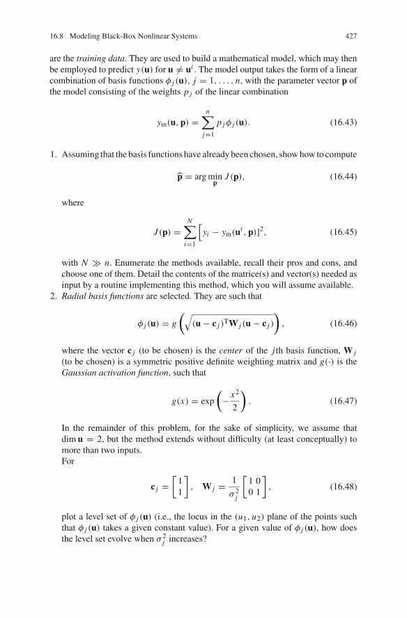
16.8 Modeling Black-Box Nonlinear Systems 427

are the training data. They are used to build a mathematical model, which may thenbe employed to predict y(u) for u ⊥= ui . The model output takes the form of a linearcombination of basis functions ρ j (u), j = 1, . . . , n, with the parameter vector p ofthe model consisting of the weights p j of the linear combination

ym(u, p) =n∑

j=1

p jρ j (u). (16.43)

1. Assuming that the basis functions have already been chosen, show how to compute

⎣p = arg minp

J (p), (16.44)

where

J (p) =N∑

i=1

⎡yi − ym(ui , p)]2, (16.45)

with N � n. Enumerate the methods available, recall their pros and cons, andchoose one of them. Detail the contents of the matrice(s) and vector(s) needed asinput by a routine implementing this method, which you will assume available.

2. Radial basis functions are selected. They are such that

ρ j (u) = g

(√(u − c j )TW j (u − c j )

), (16.46)

where the vector c j (to be chosen) is the center of the j th basis function, W j

(to be chosen) is a symmetric positive definite weighting matrix and g(·) is theGaussian activation function, such that

g(x) = exp

(− x2

2

). (16.47)

In the remainder of this problem, for the sake of simplicity, we assume thatdim u = 2, but the method extends without difficulty (at least conceptually) tomore than two inputs.For

c j =[

11

], W j = 1

α 2j

[1 00 1

], (16.48)

plot a level set of ρ j (u) (i.e., the locus in the (u1, u2) plane of the points suchthat ρ j (u) takes a given constant value). For a given value of ρ j (u), how doesthe level set evolve when α 2

j increases?

428 16 Problems

3. This very simple model may be refined, for instance by replacing p j by the j thlocal model

p j,0 + p j,1u1 + p j,2u2, (16.49)

which is linear in its parameters p j,0, p j,1, and p j,2. This leads to

ym(u, p) =n∑

j=1

(p j,0 + p j,1u1 + p j,2u2)ρ j (u), (16.50)

where the weighting function ρ j (u) specifies how much the j th local modelshould contribute to the output of the global model. This is why ρ j (·) is called anactivation function. It is still assumed that ρ j (u) is given by (16.46), with now

W j =⎤

⎥

1α 2

1, j0

0 1α 2

2, j

⎦

⎞ . (16.51)

Each of the activation functions ρ j (·) is thus specified by four parameters,namely the entries c1, j and c2, j of c j , and α 2

1, j and α 22, j , which specify W j .

The vector p now contains p j,0, p j,1 and p j,2 for j = 1, . . . , n. Assuming thatc1, j , c2, j , α

21, j , α

22, j ( j = 1, . . . , n) have been chosen a priori, show how to com-

pute⎣p that is optimal in the sense of (16.45).

16.8.2 LOLIMOT for Static Systems

The LOLIMOT method (where LOLIMOT stands for LOcal LInear MOdel Tree)provides a heuristic technique for building the activation functions ρ j (·) defined byc1, j , c2, j , α 2

1, j , α 22, j ( j = 1, . . . , n), progressively and automatically [4]. In some

initial axis-aligned rectangle of interest in parameter space, it puts a single activationfunction ( j = 1), with its center at the center of the rectangle and its parameter αi, j

(analogous to a standard deviation) equal to one-third of the length of the interval ofvariation of the input ui on this rectangle (i = 1, 2). LOLIMOT then proceeds bysuccessive bisections of rectangles of input space into subrectangles of equal surface.Each of the resulting rectangles receives its own activation function, built with thesame rules as for the initial rectangle. A binary tree is thus created, the nodes ofwhich correspond to rectangles in input space. Each bisection creates two nodes outof a parent node.

1. Assuming that the method has already created a tree with several nodes, drawthis tree and the corresponding subrectangles of the initial rectangle of interest ininput space.

16.8 Modeling Black-Box Nonlinear Systems 429

2. What criterion would you suggest for choosing the rectangle to be split?3. To avoid a combinatorial explosion of the number of rectangles, all possible bisec-

tions are considered and compared before selecting a single one of them. Whatcriterion would you suggest for comparing the performances of the candidatebisections?

4. Summarize the algorithm for an arbitrary number of inputs, and point out its prosand cons.

5. How would you deal with a system with several scalar outputs?6. Why is the method called LOLIMOT?7. Compare this approach with Kriging.

16.8.3 LOLIMOT for Dynamical Systems

1. Consider now a discrete-time single-input single-output (SISO) dynamical sys-tem, and assume that its output yk at the instant of time indexed by k can beapproximated by some (unknown) function f (·) of the n most recent past outputsand inputs, i.e.,

yk ⇒ f (vpast(k)), (16.52)

with

vpast(k) = (yk−1, . . . , yk−n, uk−1, . . . , uk−n)T. (16.53)

How can the method developed in Sect. 16.8.2 be adapted to deal with this newsituation?

2. How could it be adapted to deal with MISO dynamical systems?3. How could it be adapted to deal with MIMO dynamical systems?

16.9 Designing a Predictive Controller with l2 and l1 Norms

The scalar output y of a dynamical process is to be controlled by choosing thesuccessive values taken by its scalar input u. The input–output relationship is modeledby the discrete-time equation

ym(k, p, uk−1) =n∑

i=1

hi uk−i , (16.54)

where k is the index of the kth instant of time,

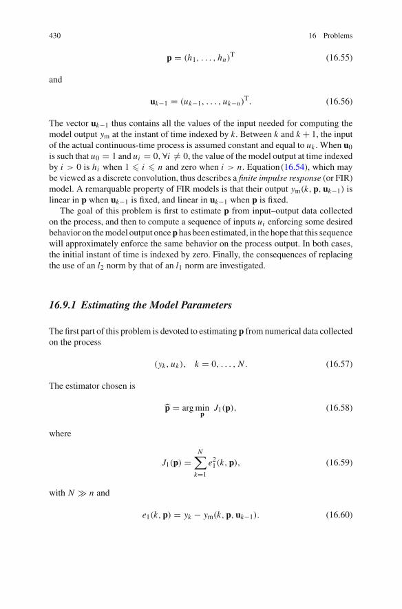
430 16 Problems

p = (h1, . . . , hn)T (16.55)

and

uk−1 = (uk−1, . . . , uk−n)T. (16.56)

The vector uk−1 thus contains all the values of the input needed for computing themodel output ym at the instant of time indexed by k. Between k and k + 1, the inputof the actual continuous-time process is assumed constant and equal to uk . When u0is such that u0 = 1 and ui = 0,∀i ⊥= 0, the value of the model output at time indexedby i > 0 is hi when 1 � i � n and zero when i > n. Equation (16.54), which maybe viewed as a discrete convolution, thus describes a finite impulse response (or FIR)model. A remarquable property of FIR models is that their output ym(k, p, uk−1) islinear in p when uk−1 is fixed, and linear in uk−1 when p is fixed.

The goal of this problem is first to estimate p from input–output data collectedon the process, and then to compute a sequence of inputs ui enforcing some desiredbehavior on the model output once p has been estimated, in the hope that this sequencewill approximately enforce the same behavior on the process output. In both cases,the initial instant of time is indexed by zero. Finally, the consequences of replacingthe use of an l2 norm by that of an l1 norm are investigated.

16.9.1 Estimating the Model Parameters

The first part of this problem is devoted to estimating p from numerical data collectedon the process

(yk, uk), k = 0, . . . , N . (16.57)

The estimator chosen is

⎣p = arg minp

J1(p), (16.58)

where

J1(p) =N∑

k=1

e21(k, p), (16.59)

with N � n and

e1(k, p) = yk − ym(k, p, uk−1). (16.60)

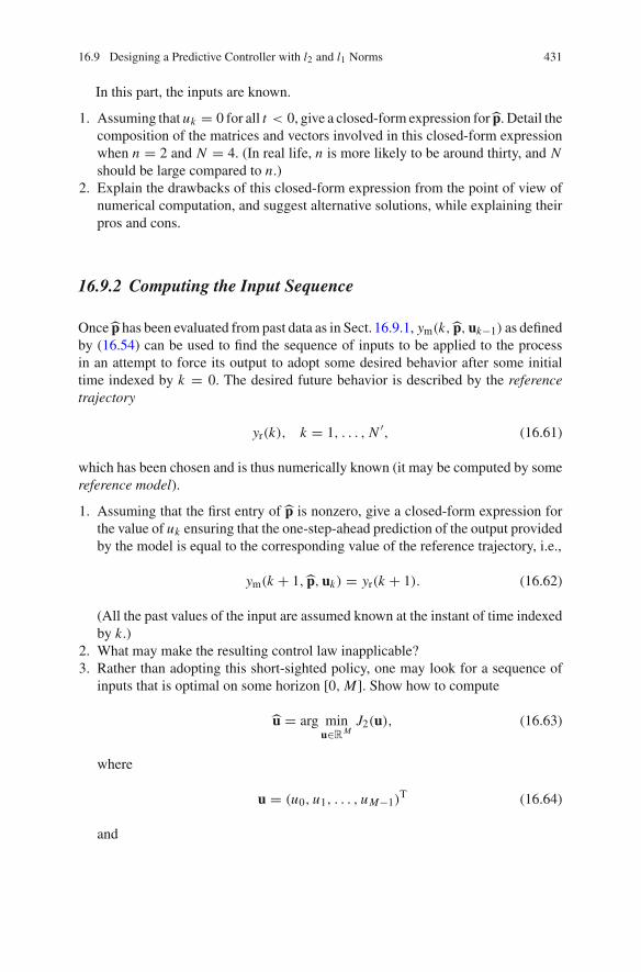
16.9 Designing a Predictive Controller with l2 and l1 Norms 431

In this part, the inputs are known.

1. Assuming that uk = 0 for all t < 0, give a closed-form expression for⎣p. Detail thecomposition of the matrices and vectors involved in this closed-form expressionwhen n = 2 and N = 4. (In real life, n is more likely to be around thirty, and Nshould be large compared to n.)

2. Explain the drawbacks of this closed-form expression from the point of view ofnumerical computation, and suggest alternative solutions, while explaining theirpros and cons.

16.9.2 Computing the Input Sequence

Once⎣p has been evaluated from past data as in Sect. 16.9.1, ym(k,⎣p, uk−1) as definedby (16.54) can be used to find the sequence of inputs to be applied to the processin an attempt to force its output to adopt some desired behavior after some initialtime indexed by k = 0. The desired future behavior is described by the referencetrajectory

yr(k), k = 1, . . . , N ∈, (16.61)

which has been chosen and is thus numerically known (it may be computed by somereference model).

1. Assuming that the first entry of⎣p is nonzero, give a closed-form expression forthe value of uk ensuring that the one-step-ahead prediction of the output providedby the model is equal to the corresponding value of the reference trajectory, i.e.,

ym(k + 1,⎣p, uk) = yr(k + 1). (16.62)

(All the past values of the input are assumed known at the instant of time indexedby k.)

2. What may make the resulting control law inapplicable?3. Rather than adopting this short-sighted policy, one may look for a sequence of

inputs that is optimal on some horizon [0, M]. Show how to compute

⎣u = arg minu→RM

J2(u), (16.63)

where

u = (u0, u1, . . . , uM−1)T (16.64)

and

432 16 Problems

J2(u) =M∑

i=1

e22(i, ui−1), (16.65)

with

e2(i, ui−1) = yr(i) − ym(i,⎣p, ui−1). (16.66)

(In (16.66) the dependency of the error e2 on⎣p is hidden, in the same way as thedependency of the error e1 on u was hidden in (16.60)). Recommend an algorithmfor computing ⎣u (and explain your choice). Detail the matrices to be providedwhen n = 2 and M = 4.

4. In practice, there are always constraints on the magnitude of the inputs that canbe applied to the process (due to the limited capabilities of the actuators as wellas for safety reasons). We assume in what follows that

|uk | � 1 ∀k. (16.67)

To avoid unfeasible inputs (and save energy), one of the possible approaches isto use a penalty function and minimize

J3(u) = J2(u) + σuTu, (16.68)

with σ > 0 chosen by the user and known numerically. Show that (16.68) can berewritten as

J3(u) = (Au − b)T (Au − b) + σuTu, (16.69)

and detail the matrice A and the vector b when n = 2 and M = 4.5. Employ the first-order optimality condition to find a closed-form expression for

⎣u = arg minu→RM

J3(u) (16.70)

for a given value of σ. How should ⎣u be computed in practice? If this strategyis viewed as a penalization, what is the corresponding constraint and what is thetype of the penalty function? What should you do if it turns out that⎣u does notcomply with (16.67)? What is the consequence of such an action on the valuetaken by J2(⎣u)?

6. Suggest an alternative approach for enforcing (16.67), and explain its pros andcons compared to the previous approach.

7. Predictive control [5], also known as Generalized Predictive Control (or GPC[6]), boils down to applying (16.70) on a receding horizon of M discrete instantsof time [7]. At time k, a sequence of optimal inputs is computed as

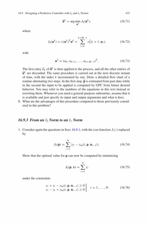
16.9 Designing a Predictive Controller with l2 and l1 Norms 433

⎣uk = arg minuk

J4(uk), (16.71)

where

J4(uk) = σ(uk)Tuk +k+M−1∑

i=k

e22(i + 1, ui ), (16.72)

with

uk = (uk, uk+1, . . . , uk+M−1)T. (16.73)

The first entry⎣uk of⎣uk is then applied to the process, and all the other entries of⎣uk are discarded. The same procedure is carried out at the next discrete instantof time, with the index k incremented by one. Draw a detailed flow chart of aroutine alternating two steps. In the first step,⎣p is estimated from past data whilein the second the input to be applied is computed by GPC from future desiredbehavior. You may refer to the numbers of the equations in this text instead orrewriting them. Whenever you need a general-purpose subroutine, assume that itis available and just specify its input and output arguments and what it does.

8. What are the advantages of this procedure compared to those previously consid-ered in this problem?

16.9.3 From an l2 Norm to an l1 Norm

1. Consider again the questions in Sect. 16.9.1, with the cost function J1(·) replacedby

J5(p) =N∑

i=1

|yi − ym(i, p, ui−1)| . (16.74)

Show that the optimal value for p can now be computed by minimizing

J6(p, x) =N∑

i=1

xi (16.75)

under the constraints

xi + yi − ym(i, p, ui−1) � 0xi − yi + ym(i, p, ui−1) � 0

}i = 1, . . . , N . (16.76)

434 16 Problems

2. What approach do you suggest for this computation? Put the problem in standardform when n = 2 and N = 4.

3. Starting from⎣p obtained by the method just described, how would you computethe sequence of inputs that minimizes

J7(u) =N∑

i=1

|yr(i) − ym(i,⎣p, ui−1)| (16.77)

under the constraints

− 1 � u(i) � 1, i = 0, . . . , N − 1, (16.78)

u(i) = 0 ∀i < 0. (16.79)

Put the problem in standard form when n = 2 and N = 4.4. What are the pros and cons of replacing the use of an l2 norm by that of an l1

norm?

16.10 Discovering and Using Recursive Least Squares

The main purpose of this problem is to study a method to take data into account assoon as they arrive in the context of linear least squares while keeping some numericalrobustness as offered by QR factorization [8]. Numerically robust real-time parameterestimation may be useful in fault detection (to detect as soon as possible that someparameters have changed) or in adaptive control (to tune the parameters of a simplemodel and the corresponding control law when the operating mode of a complexsystem changes).

The following discrete-time model is used to describe the behavior of a single-input single-output (or SISO) process

yk =n∑

i=1

ai yk−i +n∑

j=1

b j uk− j + νk . (16.80)

In (16.80), the integer n � 1 is assumed fixed beforehand. Although the general caseis considered in what follows, you may take n = 2 for the purpose of illustration,and simplify (16.80) into

yk = a1 yk−1 + a2 yk−2 + b1uk−1 + b2uk−2 + νk . (16.81)

In (16.80) and (16.81), uk is the input and yk the output, both measured on theprocess at the instant of time indexed by the integer k. The νk’s are random variables

16.10 Discovering and Using Recursive Least Squares 435

accounting for the imperfect nature of the model. They are assumed independentlyand identically distributed according to a zero-mean Gaussian law with variance α 2.Such a model is then called AutoRegressive with eXogeneous variables (or ARX).The unknown vector of parameters

p = (a1, . . . , an, b1, . . . , bn)T (16.82)

is to be estimated from the data

(yi , ui ), i = 1, . . . , N , (16.83)

where N � dim p = 2n. The estimate of p is taken as

⎣pN = arg minp→R2n

JN (p), (16.84)

where

JN (p) =N∑

i=1

[yi − ym(i, p)]2, (16.85)

with

ym(k, p) =n∑

i=1

ai yk−i +n∑

j=1

b j uk− j . (16.86)

(For the sake of simplicity, all the past values of y and u required for computingym(1, p) are assumed to be known.)

This problem consists of three parts. The first of them studies the evaluation of⎣pN from all the data (16.83) considered simultaneously. This corresponds to a batchalgorithm. The second part addresses the recursive treatment of the data, which makesit possible to take each datum into account as soon as it becomes available, withoutwaiting for data collection to be completed. The third part applies the resultingalgorithms to process control.

16.10.1 Batch Linear Least Squares

1. Show that (16.86) can be written as

ym(k, p) = fTk p, (16.87)

with fk a vector to be specified.

436 16 Problems

2. Show that (16.85) can be written as

JN (p) = ∥∥FN p − yN

∥∥22 = (FN p − yN )T(FN p − yN ), (16.88)

for a matrix FN and a vector yN to be specified. You will assume in what followsthat the columns of FN are linearly independent.

3. Let QN and RN be the matrices resulting from a QR factorization of the compositematrix

[FN |yN

]:

[FN |yN

] = QN RN . (16.89)

QN is square and orthonormal, and

RN =[

MN

O

], (16.90)

where O is a matrix of zeros. Since MN is upper triangular, it can be written as

MN =[

UN vN

0T ∂N

], (16.91)

where UN is a (2n × 2n) upper triangular matrix and 0T is a row vector of zeros.Show that

⎣pN = arg minp→R2n

∥∥∥∥MN

[p

−1

]∥∥∥∥2

2(16.92)

4. Deduce from (16.92) the linear system of equations to be solved for computing⎣pN . How do you recommend to solve it in practice?

5. How is the value of J(⎣pN ) connected to ∂N ?

16.10.2 Recursive Linear Least Squares

The information collected at the instant of time indexed by N + 1 (i.e., yN+1 anduN+1) will now be used to compute⎣pN+1 while building on the computations alreadycarried out to compute⎣pN .

1. To avoid having to increase the size of the composite matrix[FN |yN

]when N is

incremented by one, note that the first 2n rows of MN contain all the informationneeded to compute⎣pN . Append the row vector [fT

N+1 yN+1] at the end of these2n rows to form the matrix

M∈N+1 =

[UN vN

fTN+1 yN+1

]. (16.93)

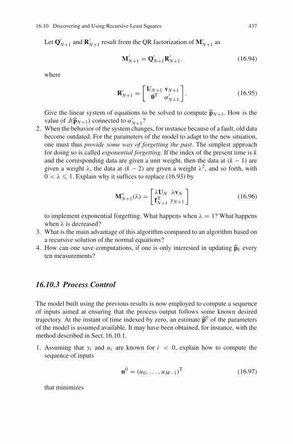
16.10 Discovering and Using Recursive Least Squares 437

Let Q∈N+1 and R∈

N+1 result from the QR factorization of M∈N+1 as

M∈N+1 = Q∈

N+1R∈N+1. (16.94)

where

R∈N+1 =

[UN+1 vN+1

0T ∂∈N+1

]. (16.95)

Give the linear system of equations to be solved to compute ⎣pN+1. How is thevalue of J(⎣pN+1) connected to ∂∈

N+1?2. When the behavior of the system changes, for instance because of a fault, old data

become outdated. For the parameters of the model to adapt to the new situation,one must thus provide some way of forgetting the past. The simplest approachfor doing so is called exponential forgetting. If the index of the present time is kand the corresponding data are given a unit weight, then the data at (k − 1) aregiven a weight σ, the data at (k − 2) are given a weight σ2, and so forth, with0 < σ � 1. Explain why it suffices to replace (16.93) by

M∈∈N+1(σ) =

[σUN σvN

fTN+1 yN+1

](16.96)

to implement exponential forgetting. What happens when σ = 1? What happenswhen σ is decreased?

3. What is the main advantage of this algorithm compared to an algorithm based ona recursive solution of the normal equations?

4. How can one save computations, if one is only interested in updating ⎣pk everyten measurements?

16.10.3 Process Control

The model built using the previous results is now employed to compute a sequenceof inputs aimed at ensuring that the process output follows some known desiredtrajectory. At the instant of time indexed by zero, an estimate⎣p0 of the parametersof the model is assumed available. It may have been obtained, for instance, with themethod described in Sect. 16.10.1.

1. Assuming that yi and ui are known for i < 0, explain how to compute thesequence of inputs

u0 = (u0, . . . , uM−1)T (16.97)

that minimizes

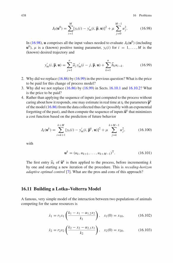
438 16 Problems

J0(u0) =M∑

i=1

[yr(i) − y∈m(i,⎣p, u)]2 + μ

M−1∑

j=0

u2j . (16.98)

In (16.98), u comprises all the input values needed to evaluate J0(u0) (includingu0), μ is a (known) positive tuning parameter, yr(i) for i = 1, . . . , M is the(known) desired trajectory and

y∈m(i,⎣p, u) =

n∑

j=1

⎣a j y∈m(i − j,⎣p, u) +

n∑

k=1

⎣bkui−k . (16.99)

2. Why did we replace (16.86) by (16.99) in the previous question? What is the priceto be paid for this change of process model?

3. Why did we not replace (16.86) by (16.99) in Sects. 16.10.1 and 16.10.2? Whatis the price to be paid?

4. Rather than applying the sequence of inputs just computed to the process withoutcaring about how it responds, one may estimate in real time at tk the parameters⎣pk

of the model (16.86) from the data collected thus far (possibly with an exponentialforgetting of the past), and then compute the sequence of inputs⎣uk that minimizesa cost function based on the prediction of future behavior

Jk(uk) =k+M∑

i=k+1

[yr(i) − y∈m(i,⎣pk, u)]2 + μ

k+M−1∑

j=k

u2j , (16.100)

with

uk = (uk, uk+1, . . . , uk+M−1)T. (16.101)

The first entry ⎣uk of ⎣uk is then applied to the process, before incrementing kby one and starting a new iteration of the procedure. This is receding-horizonadaptive optimal control [7]. What are the pros and cons of this approach?

16.11 Building a Lotka–Volterra Model

A famous, very simple model of the interaction between two populations of animalscompeting for the same resources is

x1 = r1x1

(k1 − x1 − ∂1,2x2

k1

), x1(0) = x10, (16.102)

x2 = r2x2

(k2 − x2 − ∂2,1x1

k2

), x2(0) = x20, (16.103)

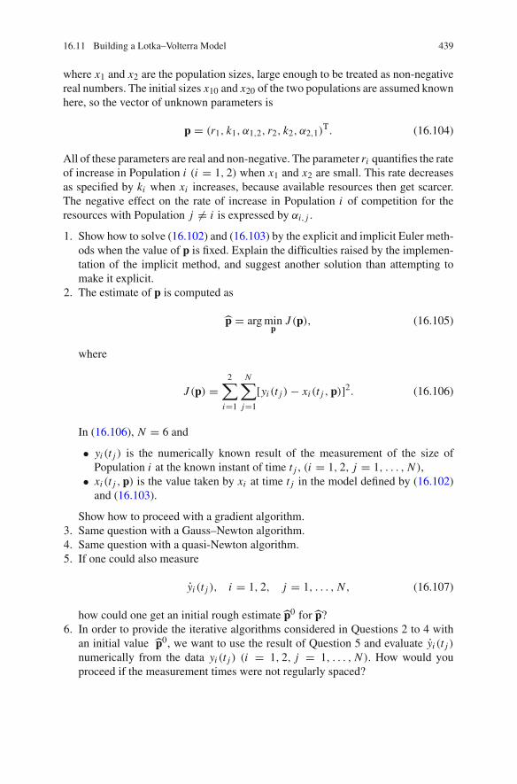
16.11 Building a Lotka–Volterra Model 439

where x1 and x2 are the population sizes, large enough to be treated as non-negativereal numbers. The initial sizes x10 and x20 of the two populations are assumed knownhere, so the vector of unknown parameters is

p = (r1, k1, ∂1,2, r2, k2, ∂2,1)T. (16.104)

All of these parameters are real and non-negative. The parameter ri quantifies the rateof increase in Population i (i = 1, 2) when x1 and x2 are small. This rate decreasesas specified by ki when xi increases, because available resources then get scarcer.The negative effect on the rate of increase in Population i of competition for theresources with Population j ⊥= i is expressed by ∂i, j .

1. Show how to solve (16.102) and (16.103) by the explicit and implicit Euler meth-ods when the value of p is fixed. Explain the difficulties raised by the implemen-tation of the implicit method, and suggest another solution than attempting tomake it explicit.

2. The estimate of p is computed as

⎣p = arg minp

J (p), (16.105)

where

J (p) =2∑

i=1

N∑

j=1

[yi (t j ) − xi (t j , p)]2. (16.106)

In (16.106), N = 6 and

• yi (t j ) is the numerically known result of the measurement of the size ofPopulation i at the known instant of time t j , (i = 1, 2, j = 1, . . . , N ),

• xi (t j , p) is the value taken by xi at time t j in the model defined by (16.102)and (16.103).

Show how to proceed with a gradient algorithm.3. Same question with a Gauss–Newton algorithm.4. Same question with a quasi-Newton algorithm.5. If one could also measure

yi (t j ), i = 1, 2, j = 1, . . . , N , (16.107)

how could one get an initial rough estimate⎣p0 for⎣p?6. In order to provide the iterative algorithms considered in Questions 2 to 4 with

an initial value ⎣p0, we want to use the result of Question 5 and evaluate yi (t j )

numerically from the data yi (t j ) (i = 1, 2, j = 1, . . . , N ). How would youproceed if the measurement times were not regularly spaced?

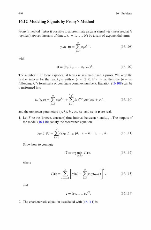
440 16 Problems

16.12 Modeling Signals by Prony’s Method

Prony’s method makes it possible to approximate a scalar signal y(t) measured at Nregularly spaced instants of time ti (i = 1, . . . , N ) by a sum of exponential terms

ym(t, θ) =n∑

j=1

a j eσ j t , (16.108)

with

θ = (a1, σ1, . . . , an, σn)T. (16.109)

The number n of these exponential terms is assumed fixed a priori. We keep thefirst m indices for the real σ j ’s, with n � m � 0. If n > m, then the (n − m)following σk’s form pairs of conjugate complex numbers. Equation (16.108) can betransformed into

ym(t, p) =m∑

j=1

a j eσ j t +

n−m2∑

k=1

bke∂k t cos(βk t + κk), (16.110)

and the unknown parameters a j , σ j , bk , ∂k , βk , and κk in p are real.

1. Let T be the (known, constant) time interval between ti and ti+1. The outputs ofthe model (16.110) satisfy the recurrence equation

ym(ti , p) =n∑

k=1

ck ym(ti−k, p), i = n + 1, . . . , N . (16.111)

Show how to compute

⎣c = arg minc→Rn

J (c), (16.112)

where

J (c) =N∑

i=n+1

[y(ti ) −

n∑

k=1

ck y(ti−k)

]2

, (16.113)

and

c = (c1, . . . , cn)T. (16.114)

2. The characteristic equation associated with (16.111) is

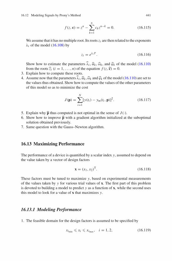
16.12 Modeling Signals by Prony’s Method 441

f (z, c) = zn −n∑

k=1

ck zn−k = 0. (16.115)

We assume that it has no multiple root. Its roots zi are then related to the exponentsσi of the model (16.108) by

zi = eσi T . (16.116)

Show how to estimate the parameters⎣σi , ⎣∂k , ⎣βk , and ⎣κk of the model (16.110)from the roots⎣zi (i = 1, . . . , n) of the equation f (z,⎣c) = 0.

3. Explain how to compute these roots.4. Assume now that the parameters⎣σi ,⎣∂k ,⎣βk and⎣κk of the model (16.110) are set to

the values thus obtained. Show how to compute the values of the other parametersof this model so as to minimize the cost

J (p) =N∑

i=1

[y(ti ) − ym(ti , p)]2. (16.117)

5. Explain why⎣p thus computed is not optimal in the sense of J (·).6. Show how to improve ⎣p with a gradient algorithm initialized at the suboptimal

solution obtained previously.7. Same question with the Gauss–Newton algorithm.

16.13 Maximizing Performance

The performance of a device is quantified by a scalar index y, assumed to depend onthe value taken by a vector of design factors

x = (x1, x2)T. (16.118)

These factors must be tuned to maximize y, based on experimental measurementsof the values taken by y for various trial values of x. The first part of this problemis devoted to building a model to predict y as a function of x, while the second usesthis model to look for a value of x that maximizes y.

16.13.1 Modeling Performance

1. The feasible domain for the design factors is assumed to be specified by

ximin � xi � ximax , i = 1, 2, (16.119)

442 16 Problems

with ximin and ximax known. Give a change of variables x∈ = f(x) that puts theconstraints under the form

− 1 � x ∈i � 1, i = 1, 2. (16.120)

In what follows, unless the initial design factors already satisfy (16.120), it isassumed that this change of variables has been performed. To simplify notation,the normalized design factors satisfying (16.120) are still called xi (i = 1, 2).

2. The four elementary experiments that can be obtained with x1 → {−1, 1} andx2 → {−1, 1} are carried out. (This is known as a two-level full factorial design.)Let y be the vector consisting of the resulting measured values of the performanceindex

yi = y(xi ), i = 1, . . . , 4. (16.121)

Show how to compute

⎣p = arg minp

J (p), (16.122)

where

J (p) =4∑

i=1

⎡y(xi ) − ym(xi , p)

⎢2, (16.123)

for the two following model structures:

ym(x, p) = p1 + p2x1 + p3x2 + p4x1x2, (16.124)

and

ym(x, p) = p1x1 + p2x2. (16.125)

In both cases, give the condition number (for the spectral norm) of the system oflinear equations associated with the normal equations. Do you recommend usinga QR or SVD factorization? Why? How would you suggest to choose betweenthese two model structures?

3. Due to the presence of measurement noise, it is deemed prudent to repeat N timeseach of the four elementary experiments of the two-level full factorial design.The dimension of y is thus now equal to 4N . What are the consequences of thisrepetition of experiments on the normal equations and on their condition number?

4. If the model structure became

ym(x, p) = p1 + p2x1 + p3x2 + p4x21 , (16.126)

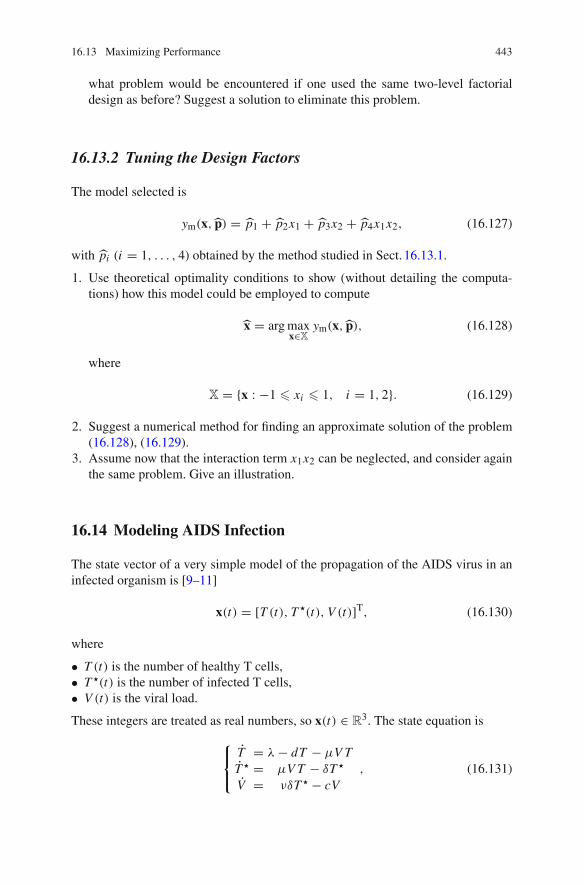
16.13 Maximizing Performance 443

what problem would be encountered if one used the same two-level factorialdesign as before? Suggest a solution to eliminate this problem.

16.13.2 Tuning the Design Factors

The model selected is

ym(x,⎣p) = ⎣p1 + ⎣p2x1 + ⎣p3x2 + ⎣p4x1x2, (16.127)

with ⎣pi (i = 1, . . . , 4) obtained by the method studied in Sect. 16.13.1.

1. Use theoretical optimality conditions to show (without detailing the computa-tions) how this model could be employed to compute

⎣x = arg maxx→X

ym(x,⎣p), (16.128)

where

X = {x : −1 � xi � 1, i = 1, 2}. (16.129)

2. Suggest a numerical method for finding an approximate solution of the problem(16.128), (16.129).

3. Assume now that the interaction term x1x2 can be neglected, and consider againthe same problem. Give an illustration.

16.14 Modeling AIDS Infection

The state vector of a very simple model of the propagation of the AIDS virus in aninfected organism is [9–11]

x(t) = [T (t), T �(t), V (t)]T, (16.130)

where

• T (t) is the number of healthy T cells,• T �(t) is the number of infected T cells,• V (t) is the viral load.

These integers are treated as real numbers, so x(t) → R3. The state equation is

T = σ − dT − μV TT � = μV T − δT �

V = νδT � − cV, (16.131)

444 16 Problems

and the initial conditions x(0) are assumed known. The vector of unknownparameters is

p = [σ, d, μ, δ, ν, c]T, (16.132)

where

• d, δ, and c are death rates,• σ is the rate of appearance of new healthy T cells,• μ is linked to the probability that a healthy T cell encountering a virus becomes

infected,• ν links virus proliferation to the death of infected T cells,• all of these parameters are real and positive.

16.14.1 Model Analysis and Simulation

1. Explain this model to someone who may not understand (16.131), in no morethan 15 lines.

2. Assuming that the value of p is known, suggest a numerical method for computingthe equilibrium solution(s). State its limitations and detail its implementation.

3. Assuming that the values of p and x(0) are known, detail the numerical integrationof the state equation by the explicit and implicit Euler methods.

4. Same question with an order-two prediction-correction method.

16.14.2 Parameter Estimation

This section is devoted to the estimation (also known as identification) of p frommeasurements carried out on a patient of the viral load V (ti ) and of the number ofhealthy T cells T (ti ) at the known instants of time ti (i = 1, . . . , N ).

1. Write down the observation equation

y(ti ) = Cx(ti ), (16.133)

where y(ti ) is the vector of the outputs measured at time ti on the patient.2. The parameter vector is to be estimated by minimizing

J (p) =N∑

i=1

[y(ti ) − Cxm(ti , p)]T[y(ti ) − Cxm(ti , p)], (16.134)

where xm(ti , p) is the result at time ti of simulating the model (16.131) for thevalue p of its parameter vector. Expand J (p) to show the state variables that are

16.14 Modeling AIDS Infection 445

measured on the patient (T (ti ), V (ti )) and those resulting from the simulation ofthe model (Tm(ti , p), Vm(ti , p)).

3. To evaluate the first-order sensitivity of the state variables of the model withrespect to the j th parameter ( j = 1, . . . , N ), it suffices to differentiate the stateequation (16.131) (and its initial conditions) with respect to this parameter. Onethus obtains another state equation (with its initial conditions), the solution ofwhich is the first-order sensitivity vector

sp j (t, p) = ∂

∂p jxm(t, p). (16.135)

Write down the state equation satisfied by the first-order sensitivity sμ(t, p) ofxm with respect to the parameter μ. What is its initial condition?

4. Assume that the first-order sensitivities of all the state variables of the modelwith respect to all the parameters have been computed with the method describedin Question 3. What method do you suggest to use to minimize J (p)? Detail itsimplementation and its pros and cons compared to other methods you might thinkof.

5. Local optimization methods based on second-order Taylor expansion encounterdifficulties when the Hessian or its approximation becomes too ill-conditioned,and this is to be feared here. How would you overcome this difficulty?

16.15 Looking for Causes

Shortly before the launch of the MESSENGER space probe from Cape Canaveral in2004, an important increase in the resistance of resistors in mission-critical circuitboards was noticed while the probe was already mounted on its launching rocketand on the launch pad [12]. Emergency experiments had to be designed to find anexplanation and decide whether the launch had to be delayed. Three factors weresuspected of having contributed to the defect:

• solder temperature (370 ∇C instead of the recommended 260 ∇C),• resistor batch,• humidity level during testing (close to 100 %).

This led to measuring resistance at 100 % humidity level (x3 = +1) and at normalhumidity level (x3 = −1), on resistors from old batches (x2 = −1) and new batches(x2 = +1), soldered at 260 ∇C (x1 = −1) or 370 ∇C (x1 = +1). Table 16.3 presentsthe resulting deviations y between the nominal and measured resistances.

1. It was decided to model y(x) by the polynomial

f (x, p) = p0 +3∑

i=1

pi xi + p4x1x2 + p5x1x3 + p6x2x3 + p7x1x2x3. (16.136)

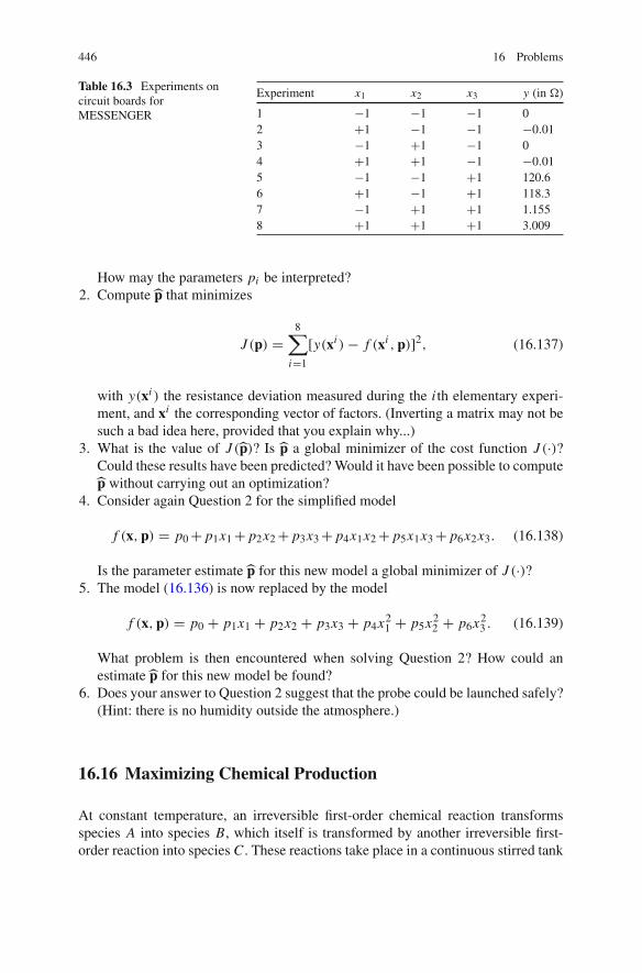
446 16 Problems

Table 16.3 Experiments oncircuit boards forMESSENGER

Experiment x1 x2 x3 y (in �)

1 −1 −1 −1 02 +1 −1 −1 −0.013 −1 +1 −1 04 +1 +1 −1 −0.015 −1 −1 +1 120.66 +1 −1 +1 118.37 −1 +1 +1 1.1558 +1 +1 +1 3.009

How may the parameters pi be interpreted?2. Compute⎣p that minimizes

J (p) =8∑

i=1

[y(xi ) − f (xi , p)]2, (16.137)

with y(xi ) the resistance deviation measured during the i th elementary experi-ment, and xi the corresponding vector of factors. (Inverting a matrix may not besuch a bad idea here, provided that you explain why...)

3. What is the value of J (⎣p)? Is ⎣p a global minimizer of the cost function J (·)?Could these results have been predicted? Would it have been possible to compute⎣p without carrying out an optimization?

4. Consider again Question 2 for the simplified model

f (x, p) = p0 + p1x1 + p2x2 + p3x3 + p4x1x2 + p5x1x3 + p6x2x3. (16.138)

Is the parameter estimate⎣p for this new model a global minimizer of J (·)?5. The model (16.136) is now replaced by the model

f (x, p) = p0 + p1x1 + p2x2 + p3x3 + p4x21 + p5x2

2 + p6x23 . (16.139)

What problem is then encountered when solving Question 2? How could anestimate⎣p for this new model be found?

6. Does your answer to Question 2 suggest that the probe could be launched safely?(Hint: there is no humidity outside the atmosphere.)

16.16 Maximizing Chemical Production

At constant temperature, an irreversible first-order chemical reaction transformsspecies A into species B, which itself is transformed by another irreversible first-order reaction into species C . These reactions take place in a continuous stirred tank

16.16 Maximizing Chemical Production 447

reactor, and the concentration of each species at any given instant of time is assumedto be the same anywhere in the reactor. The evolution of the concentrations of thequantities of interest is then described by the state equation

[ A] = −p1[A][B] = p1[A] − p2[B][C] = p2[B]

, (16.140)

where [X ] is the concentration of species X , X = A, B, C , and where p1 and p2 arepositive parameters with p1 ⊥= p2. For the initial concentrations

[A](0) = 1, [B](0) = 0, [C](0) = 0, (16.141)

it is easy to show that, for all t � 0,

[B](t, p) = p1

p1 − p2[exp(−p2t) − exp(−p1t)], (16.142)

where p =(p1, p2)T.

1. Assuming that p is numerically known, and pretending to ignore that (16.142) isavailable, show how to solve (16.140) with the initial conditions (16.141) by theexplicit and implicit Euler methods. Recall the pros and cons of the two methods.

2. One wishes to stop the reactions when [B] is maximal. Assuming again thatthe value of p is known, compute the optimal stopping time using (16.142) andtheoretical optimality conditions.

3. Assume that p must be estimated from the experimental data

y(ti ), i = 1, 2, . . . , 10, (16.143)

where y(ti ) is the result of measuring [B] in the reactor at time ti . Explain indetail how to evaluate

⎣p = arg minp

J (p), (16.144)

where

J (p) =10∑

i=1

{y(ti ) − [B](ti , p)}2, (16.145)

with [B](ti , p) the model output computed by (16.142), using the gradient, Gauss–Newton and BFGS methods, successively. State the pros and cons of each of thesemethods.

4. Replace the closed-form solution (16.142) by that provided by a numerical ODEsolver for the Cauchy problem (16.140, 16.141) and consider again the same

448 16 Problems

question with the Gauss–Newton method. (To compute the first-order sensitivitiesof [A], [B], and [C] with respect to the parameter p j

α Xj (t, p) = ∂

∂p j[X ](t, p), j = 1, 2, X = A, B, C, (16.146)

one may simulate the ODEs obtained by differentiating (16.140) with respect top j , from initial conditions obtained by differentiating (16.141) with respect top j .) Assume that a suitable ODE solver is available, without having to give detailson the matter.

5. We now wish to replace (16.145) by

J (p) =10∑

i=1

|y(ti ) − [B](ti , p)| . (16.147)

What algorithm would you recommend to evaluate⎣p, and why?

16.17 Discovering the Response-Surface Methodology

The specification sheet of a system to be designed defines the setX of all feasible val-ues for a vector x of design variables as the intersection of the half-spaces authorizedby the inequalities

aTi x � bi , i = 1, . . . , m, (16.148)

where the vectors ai and scalars bi are known numerically. An optimal value for thedesign vector is defined as

⎣x = arg minx→X

c(x). (16.149)

No closed-form expression for the cost function c(·) is available, but the numericalvalue of c(x) can be obtained for any numerical value of x by running some availablenumerical code with x as its input. The response-surface methodology [13, 14] canbe used to look for⎣x based on this information, as illustrated in this problem.

Each design variable xi belongs to the normalized interval [−1, 1], soX is a hyper-cube of width 2 centered on the origin. It is also assumed that a feasible numericalvalue⎣x0 for the design vector has already been chosen. The procedure for finding abetter numerical value of the design vector is iterative. Starting from⎣xk , it computes⎣xk+1 as suggested in the questions below.

1. For small displacements δx around⎣xk , one may use the approximation

c(⎣xk + δx) ⇒ c(⎣xk) + (δx)Tpk . (16.150)

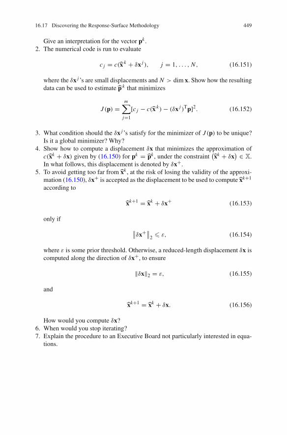
16.17 Discovering the Response-Surface Methodology 449

Give an interpretation for the vector pk .2. The numerical code is run to evaluate

c j = c(⎣x k + δx j ), j = 1, . . . , N , (16.151)

where the δx j ’s are small displacements and N > dim x. Show how the resultingdata can be used to estimate⎣p k that minimizes

J (p) =m∑

j=1

[c j − c(⎣x k) − (δx j )Tp]2. (16.152)

3. What condition should the δx j ’s satisfy for the minimizer of J (p) to be unique?Is it a global minimizer? Why?

4. Show how to compute a displacement δx that minimizes the approximation ofc(⎣xk + δx) given by (16.150) for pk = ⎣pk , under the constraint

(⎣xk + δx

) → X.In what follows, this displacement is denoted by δx+.

5. To avoid getting too far from⎣xk , at the risk of losing the validity of the approxi-mation (16.150), δx+ is accepted as the displacement to be used to compute⎣xk+1

according to

⎣xk+1 =⎣xk + δx+ (16.153)

only if

∥∥δx+∥∥2 � ν, (16.154)

where ν is some prior threshold. Otherwise, a reduced-length displacement δx iscomputed along the direction of δx+, to ensure

‖δx‖2 = ν, (16.155)

and

⎣xk+1 =⎣xk + δx. (16.156)

How would you compute δx?6. When would you stop iterating?7. Explain the procedure to an Executive Board not particularly interested in equa-

tions.

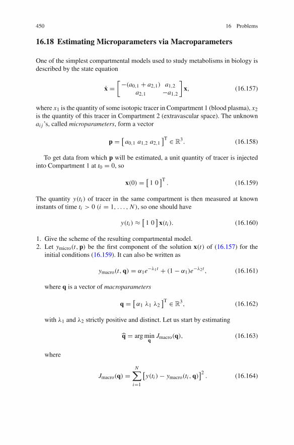
450 16 Problems

16.18 Estimating Microparameters via Macroparameters

One of the simplest compartmental models used to study metabolisms in biology isdescribed by the state equation

x =[−(a0,1 + a2,1) a1,2

a2,1 −a1,2

]x, (16.157)

where x1 is the quantity of some isotopic tracer in Compartment 1 (blood plasma), x2is the quantity of this tracer in Compartment 2 (extravascular space). The unknownai j ’s, called microparameters, form a vector

p = [a0,1 a1,2 a2,1

]T → R3. (16.158)

To get data from which p will be estimated, a unit quantity of tracer is injectedinto Compartment 1 at t0 = 0, so

x(0) = [1 0

]T. (16.159)

The quantity y(ti ) of tracer in the same compartment is then measured at knowninstants of time ti > 0 (i = 1, . . . , N ), so one should have

y(ti ) ⇒ [1 0

]x(ti ). (16.160)

1. Give the scheme of the resulting compartmental model.2. Let ymicro(t, p) be the first component of the solution x(t) of (16.157) for the

initial conditions (16.159). It can also be written as

ymacro(t, q) = ∂1e−σ1t + (1 − ∂1)e−σ2t , (16.161)

where q is a vector of macroparameters

q = [∂1 σ1 σ2

]T → R3, (16.162)

with σ1 and σ2 strictly positive and distinct. Let us start by estimating

⎣q = arg minq

Jmacro(q), (16.163)

where

Jmacro(q) =N∑

i=1

[y(ti ) − ymacro(ti , q)

]2. (16.164)

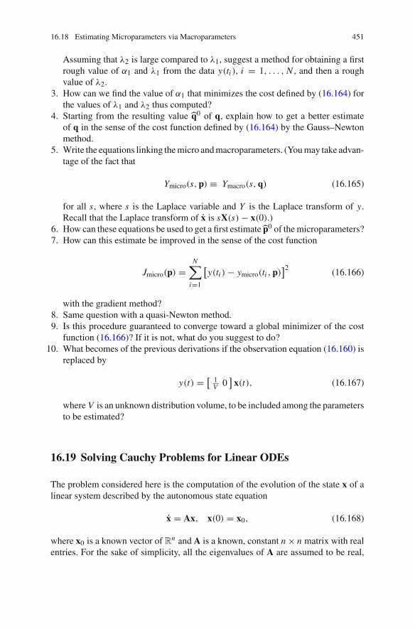
16.18 Estimating Microparameters via Macroparameters 451

Assuming that σ2 is large compared to σ1, suggest a method for obtaining a firstrough value of ∂1 and σ1 from the data y(ti ), i = 1, . . . , N , and then a roughvalue of σ2.

3. How can we find the value of ∂1 that minimizes the cost defined by (16.164) forthe values of σ1 and σ2 thus computed?

4. Starting from the resulting value ⎣q0 of q, explain how to get a better estimateof q in the sense of the cost function defined by (16.164) by the Gauss–Newtonmethod.

5. Write the equations linking the micro and macroparameters. (You may take advan-tage of the fact that

Ymicro(s, p) ∪ Ymacro(s, q) (16.165)

for all s, where s is the Laplace variable and Y is the Laplace transform of y.Recall that the Laplace transform of x is sX(s) − x(0).)

6. How can these equations be used to get a first estimate⎣p0 of the microparameters?7. How can this estimate be improved in the sense of the cost function

Jmicro(p) =N∑

i=1

[y(ti ) − ymicro(ti , p)

]2 (16.166)

with the gradient method?8. Same question with a quasi-Newton method.9. Is this procedure guaranteed to converge toward a global minimizer of the cost

function (16.166)? If it is not, what do you suggest to do?10. What becomes of the previous derivations if the observation equation (16.160) is

replaced by

y(t) = [ 1V 0

]x(t), (16.167)

where V is an unknown distribution volume, to be included among the parametersto be estimated?

16.19 Solving Cauchy Problems for Linear ODEs

The problem considered here is the computation of the evolution of the state x of alinear system described by the autonomous state equation

x = Ax, x(0) = x0, (16.168)

where x0 is a known vector of Rn and A is a known, constant n × n matrix with realentries. For the sake of simplicity, all the eigenvalues of A are assumed to be real,

452 16 Problems

negative and distinct. Mathematically, the solution is given by

x(t) = exp (At) x0, (16.169)

where the matrix exponential exp(At) is defined by the convergent series

exp(At) =√∑

i=0

1

i ! (At)i . (16.170)

Many numerical methods are available for solving (16.168). This problem is anopportunity for exploring a few of them.

16.19.1 Using Generic Methods

A first possible approach is to specialize generic methods to the linear case consideredhere.

1. Specialize the explicit Euler method. What condition should the step-size h satisfyfor the method to be stable?

2. Specialize the implicit Euler method. What condition should the step-size h satisfyfor the method to be stable?

3. Specialize a second-order Runge–Kutta method, and show that it is strictly equiv-alent to a Taylor expansion, the order of which you will specify. How can onetune the step-size h?

4. Specialize a second-order prediction-correction method combining Adams-Bashforth and Adams-Moulton.

5. Specialize a second-order Gear method.6. Suggest a simple method for estimating x(t) between ti and ti + h.

16.19.2 Computing Matrix Exponentials

An alternative approach is via the computation of matrix exponentials

1. Propose a method for computing the eigenvalues of A.2. Assuming that these eigenvalues are distinct and that you also known how to

compute the eigenvectors of A, give a similarity transformation q = Tx (with Ta constant, invertible matrix) that transforms A into

� = TAT−1, (16.171)

with � a diagonal matrix, and (16.168) into

16.19 Solving Cauchy Problems for Linear ODEs 453

q = �q, q(0) = Tx0. (16.172)

3. How can one use this result to compute x(t) for t > 0? Why is the conditionnumber of T important?

4. What are the advantages of this approach compared with the use of generic meth-ods?

5. Assume now that A is not known, and that the state is regularly measured everyh s., so x(ih) is approximately known, for i = 0, . . . , N . How can exp(Ah) beestimated? How can an estimate of A be deduced from this result?

16.20 Estimating Parameters Under Constraints

The parameter vector p = [p1, p2]T of the model

ym(tk, p) = p1 + p2tk (16.173)

is to be estimated from the experimental data y(ti ), i = 1, . . . , N , where ti and y(ti )are known numerically, by minimizing

J (p) =N∑

i=1

[y(ti ) − ym(ti , p)]2. (16.174)

1. Explain how you would proceed in the absence of any additional constraint.2. For some (admittedly rather mysterious) reasons, the model must comply with

the constraint

p21 + p2

2 = 1, (16.175)

i.e., its parameters must belong to a circle with unit radius centered at the origin.The purpose of the rest of this problem is to consider various ways of enforcing(16.175) on the estimate⎣p of p.

a. Reparametrization approach. Find a transformation p = f(θ), where θ is ascalar unknown parameter, such that (16.175) is satisfied for any real valueof θ . Suggest a numerical method for estimating θ from the data.

b. Lagrangian approach. Write down the Lagrangian of the constrained prob-lem using a vector formulation where the sum in (16.174) is replaced by anexpression involving the vector

y = [y(t1), y(t2), . . . , y(tN )]T, (16.176)

and where the constraint (16.175) is expressed as a function of p. Usingtheoretical optimality conditions show that the optimal solution⎣p for p can

454 16 Problems

be expressed as a function of the Lagrange parameter σ. Suggest at least onemethod for solving for σ the equation expressing that⎣p(σ) satisfies (16.175).

c. Penalization approach. Two strategies are being considered. The first oneemploys the penalty function

κ1(p) = |pTp − 1|, (16.177)

and the second the penalty function

κ2(p) = (pTp − 1)2. (16.178)

Describe in some detail how you would implement these strategies. What isthe difference with the Lagrangian approach? What are the pros and cons ofκ1(·) and κ2(·)? Which of the optimization methods described in this bookcan be used with κ1(·)?

d. Projection approach. In this approach, two steps are alternated. The firststep uses some unconstrained iterative method to compute an estimate⎣pk+of the solution at iteration k + 1 from the constrained estimate ⎣pk of thesolution at iteration k, while the second computes ⎣pk+1 by projecting ⎣pk+orthogonally onto the curve defined by (16.175). Explain how you wouldimplement this option in practice. Why should one avoid using the linearleast-square approach for the first step?

e. Any other idea? What are the pros and cons of these approaches?

16.21 Estimating Parameters with lp Norms

Assume that a vector of data y → RN has been collected on a system of interest.

These experimental data are modeled as

ym(x) = Fx, (16.179)

where x → Rn is a vector of unknown parameters (n < N ), and where F is an N × n

matrix with known real entries. Define the error vector as

e(x) = y − ym(x). (16.180)

This problem addresses the computation of

⎣x = arg minx

‖e(x)‖p , (16.181)

where ‖ · ‖p is the l p norm, for p = 1, 2 and +√. Recall that

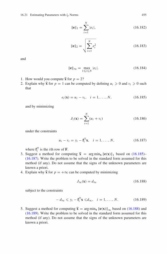
16.21 Estimating Parameters with lp Norms 455

‖e‖1 =N∑

i=1

|ei |, (16.182)

‖e‖2 =√√√√

N∑

i=1

e2i (16.183)

and

‖e‖√ = max1�i�N

|ei |. (16.184)

1. How would you compute⎣x for p = 2?2. Explain why⎣x for p = 1 can be computed by defining ui � 0 and vi � 0 such

that

ei (x) = ui − vi , i = 1, . . . , N , (16.185)

and by minimizing

J1(x) =N∑

i=1

(ui + vi ) (16.186)

under the constraints

ui − vi = yi − fTi x, i = 1, . . . , N , (16.187)

where fTi is the i th row of F.

3. Suggest a method for computing ⎣x = arg minx ‖e(x)‖1 based on (16.185)–(16.187). Write the problem to be solved in the standard form assumed for thismethod (if any). Do not assume that the signs of the unknown parameters areknown a priori.

4. Explain why⎣x for p = +√ can be computed by minimizing

J√(x) = d√ (16.188)

subject to the constraints

− d√ � yi − fTi x �d√, i = 1, . . . , N . (16.189)

5. Suggest a method for computing⎣x = arg minx ‖e(x)‖√ based on (16.188) and(16.189). Write the problem to be solved in the standard form assumed for thismethod (if any). Do not assume that the signs of the unknown parameters areknown a priori.

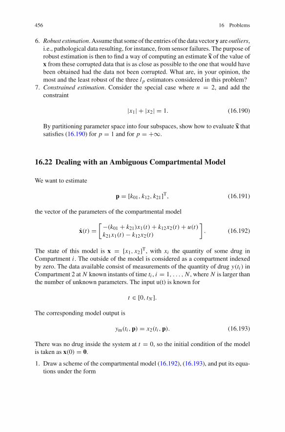
456 16 Problems

6. Robust estimation. Assume that some of the entries of the data vector y are outliers,i.e., pathological data resulting, for instance, from sensor failures. The purpose ofrobust estimation is then to find a way of computing an estimate⎣x of the value ofx from these corrupted data that is as close as possible to the one that would havebeen obtained had the data not been corrupted. What are, in your opinion, themost and the least robust of the three l p estimators considered in this problem?

7. Constrained estimation. Consider the special case where n = 2, and add theconstraint

|x1| + |x2| = 1. (16.190)

By partitioning parameter space into four subspaces, show how to evaluate⎣x thatsatisfies (16.190) for p = 1 and for p = +√.

16.22 Dealing with an Ambiguous Compartmental Model

We want to estimate

p = [k01, k12, k21]T, (16.191)

the vector of the parameters of the compartmental model

x(t) =[−(k01 + k21)x1(t) + k12x2(t) + u(t)

k21x1(t) − k12x2(t)

]. (16.192)

The state of this model is x = [x1, x2]T, with xi the quantity of some drug inCompartment i . The outside of the model is considered as a compartment indexedby zero. The data available consist of measurements of the quantity of drug y(ti ) inCompartment 2 at N known instants of time ti , i = 1, . . . , N , where N is larger thanthe number of unknown parameters. The input u(t) is known for

t → [0, tN ].

The corresponding model output is

ym(ti , p) = x2(ti , p). (16.193)

There was no drug inside the system at t = 0, so the initial condition of the modelis taken as x(0) = 0.

1. Draw a scheme of the compartmental model (16.192), (16.193), and put its equa-tions under the form

16.22 Dealing with an Ambiguous Compartmental Model 457

x = A(p)x + bu, (16.194)

ym(t, p) = cTx(t). (16.195)

2. Assuming, for the time being, that the numerical value of p is known, describetwo strategies for evaluating ym(ti , p) for i = 1, . . . , N . Without going into toomuch detail, indicate the problems to be solved for implementing these strategies,point out their pros and cons, and explain what your choice would be, and why.

3. To take measurement noise into account, p is estimated by minimizing

J (p) =N∑

i=1

[y(ti ) − ym(ti , p)]2. (16.196)

Describe two strategies for searching for the optimal value ⎣p of p, indicate theproblems to be solved for implementing them, point out their pros and cons, andexplain what your choice would be, and why.

4. The transfer function of the model (16.194,16.195) is given by

H(s, p) = cT[sI − A(p)]−1b, (16.197)

where s is the Laplace variable and I the identity matrix of appropriate dimension.For any given numerical value of p, the Laplace transform Ym(s, p) of the modeloutput ym(t, p) is obtained from the Laplace transform U (s) of the input u(t) as

Ym(s, p) = H(s, p)U (s), (16.198)

so H(s, p) characterizes the input–output behavior of the model. Show that foralmost any value p� of the vector of the model parameters, there exists anothervalue p∈ such that

∀s, H(s, p∈) = H(s, p�). (16.199)

What is the consequence of this on the number of global minimizers of thecost function J (·)? What can be expected when a local optimization methodis employed to minimize J (p)?

16.23 Inertial Navigation

An inertial measurement unit (or IMU) is used to locate a moving body in whichit is embedded. An IMU may be used in conjunction with a GPS or may replace itentirely when a GPS cannot be used (as in deep-diving submarines). IMUs comein two flavors. In the first one, a gimbal suspension is used to keep the orientationof the unit constant in an inertial (or Galilean) frame. In the second one, the unit

458 16 Problems

is strapped down on the moving body and thus fixed in the reference frame of thisbody. Strapdown IMUs tends to replace gimballed ones, as they are more robust andless expensive. Computations are then needed to compensate for the rotations of thestrapdown IMU due to motion.

1. Assume first that a vehicle has to be located during a mission on the plane (2Dversion), using a gimballed IMU that is stabilized in a local navigation frame(considered as inertial). In this IMU, two sensors measure forces and convertthem into accelerations aN (ti ) and aE (ti ) in the North and East directions, atknown instants of time ti (i = 1, . . . , N ). It is assumed that ti+1 − ti = �twhere �t is known and constant. Suggest a numerical method to evaluate theposition x(ti ) = (xN (ti ), xE (ti ))T and speed v(ti ) = (vN (ti ), vE (ti ))T of thevehicle (i = 1, . . . , N ) in the inertial frame. You will assume that the initialconditions x(t0) = (xN (t0), xE (t0))T and v(t0) = (vN (t0), vE (t0))T have beenmeasured at the start of the mission and are available. Explain your choice.

2. The IMU is now strapped down on the vehicle (still moving on a plane), andmeasures its axial and lateral accelerations ax (ti ) and ay(ti ). Let ψ(ti ) be theangle at time ti between the axis of the vehicle and the North direction (assumedto be measured by a compass, for the time being). How can one evaluate theposition x(ti ) = (xN (ti ), xE (ti ))T and speed v(ti ) = (vN (ti ), vE (ti ))T of thevehicle (i = 1, . . . , N ) in the inertial frame? The rotation matrix

R(ti ) =[

cos ψ(ti ) − sin ψ(ti )sin ψ(ti ) cos ψ(ti )

](16.200)

can be used to transform the vehicle frame into a local navigation frame, whichwill be considered as inertial.

3. Consider the previous question again, assuming now that instead of measuringψ(ti ) with a compass, one measures the angular speed of the vehicle

β(ti ) = dψ

dt(ti ). (16.201)

with a gyrometer.4. Consider the same problem with a 3D strapdown IMU to be used for a mission in

space. This IMU employs three gyrometers to measure the first derivatives withrespect to time of the roll θ , pitch ψ and yaw ρ of the vehicle. You will no longerneglect the fact that the local navigation frame is not an inertial frame. Instead, youwill assume that the formal expressions of the rotation matrix R1(θ, ψ, ρ) thattransforms the vehicle frame into an inertial frame and of the matrix R2(x, y)

that transforms the local navigation frame of interest (longitude x , latitude y,altitude z) into the inertial frame are available. What are the consequences on thecomputations of the fact that R1(θ, ψ, ρ) and R2(x, y) are orthonormal matrices?

5. Draw a block diagram of the resulting system.

16.24 Modeling a District Heating Network 459

Table 16.4 Heat-production cost

Q p 5 8 11 14 17 20 23 26

cprod 5 9 19 21 30 42 48 63

16.24 Modeling a District Heating Network

This problem is devoted to the modeling of a few aspects of a (tiny) district heatingnetwork, with

• two nodes: A to the West and B to the East,• a central branch, with a mass flow of water m0 from A to B,• a northern branch, with a mass flow of water m1 from B to A,• a southern branch, with a mass flow of water m2 from B to A.

All mass flows are in kg·s−1. The network description is considerably simplified, andthe use of such a model for the optimization of operating conditions is not considered(see [15] and [16] for more details).

The central branch includes a pump and the secondary circuit of a heat exchanger,the primary circuit of which is connected to an energy supplier. The northern branchcontains a valve to modulate m1 and the primary circuit of another heat exchanger,the secondary circuit of which is connected to a first energy consumer. The southernbranch contains only the primary circuit of a third heat exchanger, the secondarycircuit of which is connected to a second energy consumer.

16.24.1 Schematic of the Network

Draw a block diagram of the network based on the previous description and incor-porating the energy supplier, the pump, the valve, the two consumers, and the threeheat exchangers.

16.24.2 Economic Model

Measurements of production costs have produced Table 16.4, where cprod is the cost(in currency units per hour) of heat production and Qp is the produced power (inMW, a control input):

The following model is postulated for describing these data:

cprod(Qp) = a2(Qp)2 + a1 Qp + a0. (16.202)

460 16 Problems

Suggest a numerical method for estimating its parameters a0, a1, and a2. (Do notcarry out the computations, but give the numerical values of the matrices and vectorsthat will serve as inputs for this method.)

16.24.3 Pump Model

The increase in pressure �Hpump due to the pump (in m) is assumed to satisfy

�Hpump = g2

(m0β0

β

)2 + g1

(m0β0

β

)+ g0, (16.203)

where β is the actual pump angular speed (a control input at the disposal of thenetwork manager, in rad·s−1) and β0 is the pump (known) nominal angular speed.Assuming that you can choose β and measure m0 and the resulting �Hpump, suggestan experimental procedure and a numerical method for estimating the parametersg0, g1, and g2.

16.24.4 Computing Flows and Pressures

The pressure loss between A and B can be expressed in three ways. In the centralbranch

HB − HA = �Hpump − Z0m20, (16.204)

where Z0 is the (known) hydraulic resistance of the branch (due to friction, inm·kg−2·s2) and �Hpump is given by (16.203). In the northern branch

HB − HA = Z1

dm2

1, (16.205)

where Z1 is the (known) hydraulic resistance of the branch and d is the openingdegree of the valve (0 < d � 1). (This opening degree is another control input at thedisposal of the network manager.) Finally, in the southern branch

HB − HA = Z2m22, (16.206)

where Z2 is the (known) hydraulic resistance of the branch. The mass flows in thenetwork must satisfy

m0 = m1 + m2. (16.207)

16.24 Modeling a District Heating Network 461

Suggest a method for computing HB − HA, m0, m1, and m2 from the knowledge ofβ and d. Detail its numerical implementation.

16.24.5 Energy Propagation in the Pipes

Neglecting thermal diffusion, one can write for branch b (b = 0, 1, 2)

∂T

∂t(xb, t) + ∂bmb(t)

∂T

∂xb(xb, t) + βb(T (xb, t) − T0) = 0, (16.208)

where T (xb, t) is the temperature (in K) at the location xb in pipe b at time t , andwhere T0, ∂b, and βb are assumed known and constant. Discretizing this propagationequation (with xb = Lbi/N (i = 0, . . . , N ), where Lb is the pipe length and N thenumber of steps), show that one can get the following approximation

dxdt

(t) = A(t)x(t) + b(t)u(t) + b0T0, (16.209)

where u(t) = T (0, t) and x consists of the temperatures at the discretization pointsindexed by i (i = 1, . . . , N ). Suggest a method for solving this ODE numerically.

When thermal diffusion is no longer neglected, (16.208) becomes

∂T

∂t(xb, t) + ∂bmb(t)

∂T

∂xb(xb, t) + βb(T (xb, t) − T0) = ∂2T

∂x2 (xb, t). (16.210)

What does this change as regards (16.209)?

16.24.6 Modeling the Heat Exchangers

The power transmitted by a (counter-flow) heat exchanger can be written as

Qc = kS(T in

p − T outs ) − (T out

p − T ins )

ln(T inp − T out

s ) − ln(T outp − T in

s ), (16.211)

where the indices p and s correspond to the primary and secondary networks (withthe secondary network associated with the consumer), and the exponents in andout correspond to the inputs and outputs of the exchanger. The efficiency k of theexchanger and its exchange surface S are assumed known. Provided that the thermalpower losses between the primary and the secondary circuits are neglected, one canalso write

462 16 Problems

Qc = cmp(Tinp − T out

p ) (16.212)

at the primary network, with mp the primary mass flow and c the (known) specificheat of water (in J·kg−1·K−1), and

Qc = cms(Touts − T in

s ) (16.213)

at the secondary network, with ms the secondary mass flow. Assuming that mp, ms,T in

p , and T outs are known, show that the computation of Qc, T out

p , and T ins boils down

to solving a linear system of three equations in three unknowns. It may be useful tointroduce the (known) parameter

γ = exp

[kS

c

(1

mp− 1

ms

)]. (16.214)

What method do you recommend for solving this system?

16.24.7 Managing the Network

What additional information should be incorporated in the model of the network toallow a cost-efficient management?

16.25 Optimizing Drug Administration

The following state equation is one of the simplest models describing the fate of adrug administered intravenously into the human body

⎠x1 = −p1x1 + p2x2 + ux2 = p1x1 − (p2 + p3)x2

. (16.215)

In (16.215), the scalars p1, p2, and p3 are unkown, positive, and real parameters.The quantity of drug in Compartment i is denoted by xi (i = 1, 2), in mg, and u(t)is the drug flow into Compartment 1 at time t due to intravenous administration (inmg/min). The initial condition is x(0) = 0. The drug concentration (in mg/L) can bemeasured in Compartment 1 at N known instants of time ti (in min) (i = 1, . . . , N ).The model of the observations is thus

ym(ti , p) = 1

p4x1(ti , p), (16.216)

16.25 Optimizing Drug Administration 463

where

p = (p1, p2, p3, p4)T, (16.217)

with p4 the volume of distribution of the drug in Compartment 1, an additionalunkown, positive, real parameter (in L).

Let y(ti ) be the measured drug concentration in Compartment 1 at ti . It is assumedto satisfy

y(ti ) = ym(ti , p�) + ν(ti ), i = 1, . . . , N , (16.218)

where p� is the unknown “true” value of p and ν(ti ) combines the consequences ofthe measurement error and the approximate nature of the model.

The first part of this problem is about estimating p� for a specific patient basedon experimental data collected for a known input function u(·); the second is aboutusing the resulting model to design an input function that satisfies the requirementsof the treatment of this patient.

1. In which units should the first three parameters be expressed?2. The data to be employed for estimating the model parameters have been col-

lected using the following input. During the first minute, u(t) was maintainedconstant at 100 mg/min. During the following hour, u(t) was maintained con-stant at 20 mg/min. Although the response of the model to this input could becomputed analytically, this is not the approach to be taken here. For a step-sizeh = 0.1 min, explain in some detail how you would simulate the model and com-pute its state x(ti , p) for this specific input and for any given feasible numericalvalue of p. (For the sake of simplicity, you will assume that the measurementtimes are such that ti = ni h, with ni a positive integer.) State the pros and consof your approach, explain what simple measures you could take to check that thesimulation is reasonably accurate and state what you would do if it turned out notto be the case.

3. The estimate⎣p of p� must be computed by minimizing

J (p) =N∑

i=1

[y(ti ) − 1

p4x1(ti , p)

]2

, (16.219)

where N = 10. The instants of time ti at which the data have been collectedare known, as well as the corresponding values of y(ti ). The value of x1(ti , p)

is computed by the method that you have chosen in your answer to Question 2.Explain in some detail how you would proceed to compute⎣p. State the pros andcons of the method chosen, explain what simple measures you could take to checkwhether the optimization has been carried out satisfactorily and state what youwould do if it turned out not to be the case.

4. From now on, p is taken equal to ⎣p, the vector of numerical values obtained atQuestion 3, and the problem is to choose a therapeutically appropriate one-hour

464 16 Problems

intravenous administration profile. This hour is partitioned into 60 one-minuteintervals, and the input flow is maintained constant during any given one of thesetime intervals. Thus

u(τ ) = ui ∀τ → [(i − 1), i] min, i = 1, . . . , 60, (16.220)

and the input is uniquely specified by u → R60. Let x j (u1) be the model state

at time jh ( j = 1, . . . , 600), computed with a fixed step-size h = 0.1 minfrom x(0) = 0 for the input u1 such that u1

1 = 1 and u1i = 0, i = 2, . . . , 60.

Taking advantage of the fact that the output of the model described by (16.215)is linear in its inputs and time-invariant, express the state x j (u) of the model attime jh for a generic input u as a linear combination of suitably delayed xk(u1)’s(k = 1, . . . , 600).

5. The input u should be such that

• ui � 0, i = 1, . . . , 60 (why?),• x j

i � Mi , j = 1, . . . , 600, where Mi is a known toxicity bound (i = 1, 2),

• x j2 → [m−, m+], j = 60, . . . , 600, where m− and m+ are the known bounds

of the therapeutic range for the patient under treatment (with m+ < M2),• the total quantity of drug ingested during the hour is minimal.

Explain in some detail how to proceed and how the problem could be expressed instandard form. Under which conditions is the method that you suggest guaranteedto provide a solution (at least from a mathematical point of view)? If a solution⎣uis found, will it be a local or a global minimizer?

16.26 Shooting at a Tank

The action takes place in a two-dimensional battlefield, where position is indicatedby the value of x and altitude by that of y. On a flat, horizontal piece of land, a cannonhas been installed at (x = 0, y = 0) and its gunner has received the order to shootat an enemy tank. The modulus v0 of the shell initial velocity is fixed and known,and the gunner must only choose the aiming angle θ in the open interval

(0, π

2

). In

the first part of the problem, the tank stands still at (x = xtank > 0, y = 0), and thegunner knows the value of xtank, provided to him by a radar.

1. Neglecting drag, and assuming that the cannon is small enough for the initialposition of the shell to be taken as (x = 0, y = 0), show that the shell altitudebefore impact satisfies (for t � t0)

yshell(t) = v0 sin(θ)(t − t0) − g

2(t − t0)

2, (16.221)

with g the gravitational acceleration and t0 the instant of time at which the cannonwas fired. Show also that the horizontal distance covered by the shell before impactis

16.26 Shooting at a Tank 465

xshell(t) = v0 cos(θ)(t − t0). (16.222)

2. Explain why choosing θ to hit the tank can be viewed as a two endpoint boundary-value problem, and suggest a numerical method for computing θ . Explain whythe number of solutions may be 0, 1, or 2, depending on the position of the tank.

3. From now on, the tank may be moving. The radar indicates its position xtank(ti ),i = 1, . . . , N , at a rate of one measurement per second. Suggest a numeri-cal method for evaluating the tank instantaneous speed xtank(t) and accelerationxtank(t) based on these measurements. State the pros and cons of this method.

4. Suggest a numerical method based on the estimates obtained in Question 3 forchoosing θ and t0 in such a way that the shell hits the ground where the tank isexpected to be at the instant of impact.

16.27 Sparse Estimation Based on POCS

A vector y of experimental data

yi → R, i = 1, . . . , N , (16.223)

with N large, is to be approximated by a vector ym(p) of model outputs ym(i, p),where

ym(i, p) = fTi p, (16.224)

with fi → Rn a known regression vector and p → R

n a vector of unknown parametersto be estimated. It is assumed that

yi = ym(i, p�) + vi , (16.225)

where p� is the (unknown) “true” value of the parameter vector and vi is the mea-surement noise. The dimension n of p is very large. It may even be so large thatn > N . Estimating p� from the data then seems hopeless, but can still be carried outif some hypotheses restrict the choice. We assume in this problem that the model issparse, in the sense that the number of nonzero entries in p� is very small comparedto the dimension of p. This is relevant for many situations in signal processing.

A classical method for looking for a sparse estimate of p� is to compute

⎣p = arg minp

⎡‖y − ym(p)‖2

2 + σ‖p‖1

⎢, (16.226)

with σ a positive hyperparameter (hyperparameters are parameters of the algorithm,to be tuned by the user). The penalty function ‖p‖1 is known to promote sparsity.Computing ⎣p is not trivial, however, as the l1 norm is not differentiable and thedimension of p is very large.

466 16 Problems

The purpose of this problem is to explore an alternative approach [17] for buildinga sparsity-promoting algorithm. This approach is based on projections onto convexsets (or POCS). Let C be a convex set in R

n . For each p → Rn , there is a unique

p∇ → Rn such that

p∇ = arg minq→C

‖p − q‖22. (16.227)

This vector is the result of the projection of p onto C, denoted by

p∇ = PC(p). (16.228)

1. Illustrate the projection (16.228) for n = 2, assuming that C is rectangular.Distinguish when p belongs to C from when it does not.

2. Assume that a bound b is available for the acceptable absolute error between thei th datum yi and the corresponding model output ym(i, p), which amounts toassuming that the measurement noise is such that |vi | � b. The value of b maybe known or considered as a hyperparameter. The pair (yi , fi ) is then associatedwith a feasible slab in parameter space, defined as

Si ={

p → Rn : −b � yi − fT

i p � b}

. (16.229)

Illustrate this for n = 2 (you may try n = 3 if you feel gifted for drawings...).Show that Si is a convex set.

3. Given the data (yi , fi ), i = 1, . . . , N , and the bound b, the set S of all acceptablevalues of p is the intersection of all these feasible slabs

S =N⋂

i=1

Si . (16.230)

Instead of looking for ⎣p that minimizes some cost function, as in (16.226), welook for the estimate pk+1 of p� by projecting pk onto Sk+1, k = 0, . . . , N − 1.Thus, from some initial value p0 assumed to be available, we compute

p1 = PS1(p0),

p2 = PS2(p1) = PS2(PS1(p

0)), (16.231)

and so forth. (A more efficient procedure is based on convex combinations ofpast projections; it will not be considered here.) Using the stationarity of theLagrangian of the cost

J (p) = ‖p − pk‖22 (16.232)

with the constraints

16.27 Sparse Estimation Based on POCS 467

− b � yk+1 − fTk+1p � b, (16.233)

show how to compute pk+1 as a function of pk, yk+1, fk+1, and b, and illustratethe procedure for n = 2.

4. Sparsity still needs to be promoted. A natural approach for doing so would be toreplace pk+1 at each iteration by its projection onto the set

B0(c) = {p → R

n : ‖p‖0 � c}, (16.234)

where c is a hyperparameter and ‖p‖0 is the “l0 norm” of p, defined as the numberof its nonzero entries. Explain why l0 is not a norm.

5. Draw the set B0(c) for n = 2 and c = 1, assuming that |p j | � 1, j = 1, . . . , n.Is this set convex?

6. Draw the sets

B1(c) = {p → R

n : ‖p‖1 � c},B2(c) = {

p → Rn : ‖p‖2 � c},

B√(c) = {p → R

n : ‖p‖√ � c}, (16.235)

for n = 2 and c = 1. Are they convex? Which of the l p norms gives the closestresult to that of Question 5?

7. To promote sparsity, pk+1 is replaced at each iteration by its projection ontoB1(c),with c a hyperparameter. Explain how this projection can be carried out with aLagrangian approach and illustrate the procedure when n = 2.

8. Summarize an algorithm based on POCS for estimating p� while promoting spar-sity.

9. Is there any point in recirculating the data in this algorithm?

References

1. Langville, A., Meyer, C.: Google’s PageRank and Beyond. Princeton University Press, Prince-ton (2006)

2. Chang, J., Guo, Z., Fortmann, R., Lao, H.: Characterization and reduction of formaldehydeemissions from a low-VOC latex paint. Indoor Air 12(1), 10–16 (2002)

3. Thomas, L., Mili, L., Shaffer, C., Thomas, E.: Defect detection on hardwood logs using highresolution three-dimensional laser scan data. In: IEEE International Conference on ImageProcessing, vol. 1, pp. 243–246. Singapore (2004)

4. Nelles, O.: Nonlinear System Identification. Springer, Berlin (2001)5. Richalet, J., Rault, A., Testud, J., Papon, J.: Model predictive heuristic control: applications to

industrial processes. Automatica 14, 413–428 (1978)6. Clarke, D., Mohtadi, C., Tuffs, P.: Generalized predictive control—part I. The basic algorithm.

Automatica 23(2), 137–148 (1987)7. Bitmead, R., Gevers, M., Wertz, V.: Adaptive Optimal Control, the Thinking Man’s GPC.

Prentice-Hall, Englewood Cliffs (1990)

468 16 Problems

8. Lawson, C., Hanson, R.: Solving Least Squares Problems. Classics in Applied Mathematics.SIAM, Philadelphia (1995)

9. Perelson, A.: Modelling viral and immune system dynamics. Nature 2, 28–36 (2002)10. Adams, B., Banks, H., Davidian, M., Kwon, H., Tran, H., Wynne, S., Rosenberg, E.: HIV

dynamics: modeling, data analysis, and optimal treatment protocols. J. Comput. Appl. Math.184, 10–49 (2005)

11. Wu, H., Zhu, H., Miao, H., Perelson, A.: Parameter identifiability and estimation of HIV/AIDSdynamic models. Bull. Math. Biol. 70, 785–799 (2008)

12. Spall, J.: Factorial design for efficient experimentation. IEEE Control Syst. Mag. 30(5), 38–53(2010)

13. del Castillo, E.: Process Optimization: A Statistical Approach. Springer, New York (2007)14. Myers, R., Montgomery, D., Anderson-Cook, C.: Response Surface Methodology: Process and

Product Optimization Using Designed Experiments, 3rd edn. Wiley, Hoboken (2009)15. Sandou, G., Font, S., Tebbani, S., Hiret, A., Mondon, C.: District heating: a global approach to

achieve high global efficiencies. In: IFAC Workshop on Energy Saving Control in Plants andBuidings. Bansko, Bulgaria (2006)

16. Sandou, G., Font, S., Tebbani, S., Hiret, A., Mondon, C.: Optimisation and control of supplytemperatures in district heating networks. In: 13rd IFAC Workshop on Control Applications ofOptimisation. Cachan, France (2006)

17. Theodoridis, S., Slavakis, K., Yamada, I.: Adaptive learning in a world of projections. IEEESignal Process. Mag. 28(1), 97–123 (2011)

Index

AAbsolute stability, 316Active constraint, 170, 253Adams-Bashforth methods, 310Adams-Moulton methods, 311Adapting step-size

multistep methods, 322one-step methods, 320

Adaptive quadrature, 101Adaptive random search, 223Adjoint code, 124, 129Angle between search directions, 202Ant-colony algorithms, 223Approximate algorithm, 381, 400Armijo condition, 198Artificial variable, 267Asymptotic stability, 306Augmented Lagrangian, 260Automatic differentiation, 120

BBackward error analysis, 389Backward substitution, 23Barrier functions, 257, 259, 277Barycentric Lagrange interpolation, 81Base, 383Basic feasible solution, 267Basic variable, 269Basis functions, 83, 334BDF methods, 311Bernstein polynomials, 333Best linear unbiased predictor (BLUP), 181Best replay, 222BFGS, 211

Big O, 11Binding constraint, 253Bisection method, 142Bisection of boxes, 394Black-box modeling, 426Boole’s rule, 104Boundary locus method, 319Boundary-value problem (BVP), 302, 328Bounded set, 246Box, 394Branch and bound, 224, 422Brent’s method, 197Broyden’s method, 150Bulirsch-Stoer method, 324Burgers equation, 360

CCasting out the nines, 390Cauchy condition, 303Cauchy-Schwarz inequality, 13Central path, 277Central-limit theorem, 400CESTAC/CADNA, 397

validity conditions, 400Chain rule for differentiation, 122Characteristic curves, 363Characteristic equation, 61Chebyshev norm, 13Chebyshev points, 81Cholesky factorization, 42, 183, 186

flops, 45Chord method, 150, 313Closed set, 246Collocation, 334, 335, 372

É. Walter, Numerical Methods and Optimization, 469DOI: 10.1007/978-3-319-07671-3,© Springer International Publishing Switzerland 2014

470 Index

Combinatorial optimization, 170, 289Compact set, 246Compartmental model, 300Complexity, 44, 272Computational zero, 399Computer experiment, 78, 225Condition number, 19, 28, 150, 186, 193

for the spectral norm, 20nonlinear case, 391preserving the, 30

Conditioning, 194, 215, 390Conjugate directions, 40Conjugate-gradient methods, 40, 213, 216Constrained optimization, 170, 245Constraints

active, 253binding, 253equality, 248getting rid of, 247inequality, 252saturated, 253violated, 253

Continuation methods, 153Contraction

of a simplex, 218of boxes, 394

Convergence speed, 15, 215linear, 215of fixed-point iteration, 149of Newton’s method, 145, 150of optimization methods, 215of the secant method, 148quadratic, 215superlinear, 215

Convex optimization, 272Cost function, 168

convex, 273non-differentiable, 216

Coupling at interfaces, 370Cramer’s rule, 22Crank–Nicolson scheme, 366Curse of dimensionality, 171Cyclic optimization, 200CZ, 399, 401

DDAE, 326Dahlquist’s test problem, 315Damped Newton method, 204Dantzig’s simplex algorithm, 266Dealing with conflicting objectives, 226, 246Decision variable, 168

Deflation procedure, 65Dependent variables, 121Derivatives

first-order, 113second-order, 116

Design specifications, 246Determinant evaluation

bad idea, 3useful?, 60via LU factorization, 60via QR factorization, 61via SVD, 61

Diagonally dominant matrix, 22, 36, 37, 366Dichotomy, 142Difference

backward, 113, 116centered, 114, 116first-order, 113forward, 113, 116second-order, 114

Differentiable cost, 172Differential algebraic equations, 326Differential evolution, 223Differential index, 328Differentiating

multivariate functions, 119univariate functions, 112

Differentiationbackward, 123, 129forward, 127, 130

Direct code, 121Directed rounding, 385

switched, 391Dirichlet conditions, 332, 361Divide and conquer, 224, 394, 422Double, 384Double float, 384Double precision, 384Dual problem, 276Dual vector, 124, 275Duality gap, 276Dualization, 124

order of, 125

EEBLUP, 182Efficient global optimization (EGO), 225, 280Eigenvalue, 61, 62

computation via QR iteration, 67Eigenvector, 61, 62

computation via QR iteration, 68Elimination of boxes, 394

Index 471

Elliptic PDE, 363Empirical BLUP, 182Encyclopedias, 409eps, 154, 386Equality constraints, 170Equilibrium points, 141Euclidean norm, 13Event function, 304Exact finite algorithm, 3, 380, 399Exact iterative algorithm, 380, 400Existence and uniqueness condition, 303Expansion of a simplex, 217Expected improvement, 225, 280Explicit Euler method, 306Explicit methods

for ODEs, 306, 308, 310for PDEs, 365

Explicitation, 307an alternative to, 313

Exponent, 383Extended state, 301Extrapolation, 77

Richardson’s, 88

FFactorial design, 186, 228, 417, 442Feasible set, 168

convex, 273desirable properties of, 246

Finite difference, 306, 331Finite difference method (FDM)

for ODEs, 331for PDEs, 364

Finite element, 369Finite escape time, 303Finite impulse response model, 430Finite-element method (FEM), 368FIR, 430Fixed-point iteration, 143, 148Float, 384Floating-point number, 383Flop, 44Forward error analysis, 389Forward substitution, 24Frobenius norm, 15, 42Functional optimization, 170

GGalerkin methods, 334Gauss-Lobatto quadrature, 109Gauss-Newton method, 205, 215

Gauss-Seidel method, 36Gaussian activation function, 427Gaussian elimination, 25Gaussian quadrature, 107Gear methods, 311, 325General-purpose ODE integrators, 305Generalized eigenvalue problem, 64Generalized predictive control (GPC), 432Genetic algorithms, 223Givens rotations, 33Global error, 324, 383Global minimizer, 168Global minimum, 168Global optimization, 222GNU, 412Golden number, 148Golden-section search, 198GPL, 412GPU, 46Gradient, 9, 119, 177

evaluation by automatic differentiation, 120evaluation via finite differences, 120evaluation via sensitivity functions, 205

Gradient algorithm, 202, 215stochastic, 221

Gram-Schmidt orthogonalization, 30Grid norm, 13Guaranteed

integration of ODEs, 309, 324optimization, 224

HHeat equation, 363, 366Hessian, 9, 119, 179

computation of, 129Heun’s method, 314, 316Hidden bit, 384Homotopy methods, 153Horner’s algorithm, 81Householder transformation, 30Hybrid systems, 304Hyperbolic PDE, 363

IIEEE 754, 154, 384Ill-conditioned problems, 194Implicit Euler method, 306Implicit methods

for ODEs, 306, 311, 313for PDEs, 365

Inclusion function, 393

472 Index

Independent variables, 121Inequality constraints, 170Inexact line search, 198Infimum, 169Infinite-precision computation, 383Infinity norm, 14Initial-value problem, 302, 303Initialization, 153, 216Input factor, 89Integer programming, 170, 289, 422Integrating functions

multivariate case, 109univariate case, 101via the solution of an ODE, 109

Interior-point methods, 271, 277, 291Interpolation, 77

by cubic splines, 84by Kriging, 90by Lagrange’s formula, 81by Neville’s algorithm, 83multivariate case, 89polynomial, 18, 80, 89rational, 86univariate case, 79

Interval, 392computation, 392Newton method, 396vector, 394

Inverse power iteration, 65Inverting a matrix

flops, 60useful?, 59via LU factorization, 59via QR factorization, 60via SVD, 60

Iterativeimprovement, 29optimization, 195solution of linear systems, 35solution of nonlinear systems, 148

IVP, 302, 303

JJacobi iteration, 36Jacobian, 9Jacobian matrix, 9, 119

KKarush, Kuhn and Tucker conditions, 256Kriging, 79, 81, 90, 180, 225

confidence intervals, 92

correlation function, 91data approximation, 93mean of the prediction, 91variance of the prediction, 91

Kronecker delta, 188Krylov subspace, 39Krylov subspace iteration, 38Kuhn and Tucker coefficients, 253

Ll1 norm, 13, 263, 433l2 norm, 13, 184l p norm, 12, 454l∞ norm, 13, 264Lagrange multipliers, 250, 253Lagrangian, 250, 253, 256, 275

augmented, 260LAPACK, 28Laplace’s equation, 363Laplacian, 10, 119Least modulus, 263Least squares, 171, 183

for BVPs, 337formula, 184recursive, 434regularized, 194unweighted, 184via QR factorization, 188via SVD, 191weighted, 183when the solution is not unique, 194

Legendre basis, 83, 188Legendre polynomials, 83, 107Levenberg’s algorithm, 209Levenberg-Marquardt algorithm, 209, 215Levinson-Durbin algorithm, 43Line search, 196

combining line searches, 200Linear convergence, 142, 215Linear cost, 171Linear equations, 139

solving large systems of, 214system of, 17

Linear ODE, 304Linear PDE, 366Linear programming, 171, 261, 278Lipschitz condition, 215, 303Little o, 11Local method error

estimate of, 320for multistep methods, 310of Runge-Kutta methods, 308

Index 473

Local minimizer, 169Local minimum, 169Logarithmic barrier, 259, 272, 277, 279LOLIMOT, 428Low-discrepancy sequences, 112LU factorization, 25

flops, 45for tridiagonal systems, 44

Lucky cancelation, 104, 105, 118

MMachine epsilon, 154, 386Manhattan norm, 13Mantissa, 383Markov chain, 62, 415Matrix

derivatives, 8diagonally dominant, 22, 36, 332exponential, 304, 452inverse, 8inversion, 22, 59non-negative definite, 8normal, 66norms, 14orthonormal, 27permutation, 27positive definite, 8, 22, 42product, 7singular, 17sparse, 18, 43, 332square, 17symmetric, 22, 65Toeplitz, 23, 43triangular, 23tridiagonal, 18, 22, 86, 368unitary, 27upper Hessenberg, 68Vandermonde, 43, 82

Maximum likelihood, 182Maximum norm, 13Mean-value theorem, 395Mesh, 368Meshing, 368Method error, 88, 379, 381

bounding, 396local, 306

MIMO, 89Minimax estimator, 264Minimax optimization, 222

on a budget, 226Minimizer, 168Minimizing an expectation, 221

Minimum, 168MISO, 89Mixed boundary conditions, 361Modified midpoint integration method, 324Monte Carlo integration, 110Monte Carlo method, 397MOOCs, 414Multi-objective optimization, 226Multiphysics, 362Multistart, 153, 216, 223Multistep methods for ODEs, 310Multivariate systems, 141

N1-norm, 142-norm, 14Nabla operator, 10NaN, 384Necessary optimality condition, 251, 253Nelder and Mead algorithm, 217Nested integrations, 110Neumann conditions, 361Newton contractor, 395Newton’s method, 144, 149, 203, 215, 257,

278, 280damped, 147, 280for multiple roots, 147

Newton-Cotes methods, 102No free lunch theorems, 172Nonlinear cost, 171Nonlinear equations, 139

multivariate case, 148univariate case, 141

Nordsieck vector, 323Normal equations, 186, 337Normalized representation, 383Norms, 12

compatible, 14, 15for complex vectors, 13for matrices, 14for vectors, 12induced, 14subordinate, 14

Notation, 7NP-hard problems, 272, 291Number of significant digits, 391, 398Numerical debugger, 402

OObjective function, 168ODE, 299

scalar, 301

474 Index

Off-base variable, 269OpenCourseWare, 413Operations on intervals, 392Operator overloading, 129, 392, 399Optimality condition

necessary, 178, 179necessary and sufficient, 275, 278sufficient local, 180

Optimization, 168combinatorial, 289in the worst case, 222integer, 289linear, 261minimax, 222nonlinear, 195of a non-differentiable cost, 224on a budget, 225on average, 220

Orderof a method error, 88, 106of a numerical method, 307of an ODE, 299

Ordinary differential equation, 299Outliers, 263, 425Outward rounding, 394Overflow, 384

PPageRank, 62, 415Parabolic interpolation, 196Parabolic PDE, 363Pareto front, 227Partial derivative, 119Partial differential equation, 359Particle-swarm optimization, 223PDE, 359Penalty functions, 257, 280Perfidious polynomial, 72Performance index, 168Periodic restart, 212, 214Perturbing computation, 397Pivoting, 27Polack-Ribière algorithm, 213Polynomial equation

nth order, 64companion matrix, 64second-order, 3

Polynomial regression, 185Powell’s algorithm, 200Power iteration algorithm, 64Preconditioning, 41Prediction method, 306

Prediction-correction methods, 313Predictive controller, 429Primal problem, 276Problems, 415Program, 261Programming, 168

combinatorial, 289integer, 289linear, 261nonlinear, 195sequential quadratic, 261

Prototyping, 79

QQR factorization, 29, 188

flops, 45QR iteration, 67

shifted, 69Quadratic convergence, 146, 215Quadratic cost, 171

in the decision vector, 184in the error, 183

Quadrature, 101Quasi steady state, 327Quasi-Monte Carlo integration, 112Quasi-Newton equation, 151, 211Quasi-Newton methods

for equations, 150for optimization, 210, 215

RRadial basis functions, 427Random search, 223Rank-one correction, 151, 152Rank-one matrix, 8realmin, 154Reflection of a simplex, 217Regression matrix, 184Regularization, 34, 194, 208Relaxation method, 222Repositories, 410Response-surface methodology, 448Richardson’s extrapolation, 88, 106, 117, 324Ritz-Galerkin methods, 334, 372Robin conditions, 361Robust estimation, 263, 425Robust optimization, 220Romberg’s method, 106Rounding, 383

modes, 385Rounding errors, 379, 385

Index 475

cumulative effect of, 386Runge phenomenon, 93Runge-Kutta methods, 308

embedded, 321Runge-Kutta-Fehlberg method, 321Running error analysis, 397

SSaddle point, 178Saturated constraint, 170, 253Scalar product, 389Scaling, 314, 383Schur decomposition, 67Schwarz’s theorem, 9Search engines, 409Secant method, 144, 148Second-order linear PDE, 361Self-starting methods, 309Sensitivity functions, 205

evaluation of, 206for ODEs, 207

Sequential quadratic programming (SQP), 261Shifted inverse power iteration, 66Shooting methods, 330Shrinkage of a simplex, 219Simplex, 217Simplex algorithm

Dantzig’s, 265Nelder and Mead’s, 217

Simpson’s 1/3 rule, 103Simpson’s 3/8 rule, 104Simulated annealing, 223, 290Single precision, 384Single-step methods for ODEs, 306, 307Singular perturbations, 326Singular value decomposition (SVD), 33, 191

flops, 45Singular values, 14, 21, 191Singular vectors, 191Slack variable, 253, 265Slater’s condition, 276Software, 411Sparse matrix, 18, 43, 53, 54, 366, 373Spectral decomposition, 68Spectral norm, 14Spectral radius, 14Splines, 84, 333, 369Stability of ODEs

influence on global error, 324Standard form

for equality constraints, 248for inequality constraints, 252

for linear programs, 265State, 122, 299State equation, 122, 299Stationarity condition, 178Steepest descent algorithm, 202Step-size

influence on stability, 314tuning, 105, 320, 322

Stewart-Gough platform, 141Stiff ODEs, 325Stochastic gradient algorithm, 221Stopping criteria, 154, 216, 400Storage of arrays, 46Strong duality, 276Strong Wolfe conditions, 199Student’s test, 398Subgradient, 217Successive over-relaxation (SOR), 37Sufficient local optimality condition, 251Superlinear convergence, 148, 215Supremum, 169Surplus variable, 265Surrogate model, 225

TTaxicab norm, 13Taylor expansion, 307

of the cost, 177, 179, 201Taylor remainder, 396Termination, 154, 216Test for positive definiteness, 43Test function, 335TeXmacs, 6Theoretical optimality conditions

constrained case, 248convex case, 275unconstrained case, 177

Time dependencygetting rid of, 301

Training data, 427Transcendental functions, 386Transconjugate, 13Transposition, 7Trapezoidal rule, 103, 311Traveling salesperson problem (TSP), 289Trust-region method, 196Two-endpoint boudary-value problems, 328Types of numerical algorithms, 379

UUnbiased predictor, 181

476 Index

Unconstrained optimization, 170, 177Underflow, 384Uniform norm, 13Unit roundoff, 386Unweighted least squares, 184Utility function, 168

VVerifiable algorithm, 3, 379, 400Vetter’s notation, 8Vibrating-string equation, 363

Violated constraint, 253

WWarm start, 258, 278Wave equation, 360Weak duality, 276WEB resources, 409Weighted least squares, 183Wolfe’s method, 198Worst operations, 405Worst-case optimization, 222