State of Rhode Island

Department of Environmental Management Office of Air Resources

Rhode Island Air Dispersion Modeling

Guidelines for Stationary Sources

March 2013 Revision

2

TABLE OF CONTENTS

Glossary of Acronyms and Symbols..........................................................................4 Definitions..................................................................................................................7 1.0 INTRODUCTION .........................................................................................11 2.0 CRITERIA POLLUTANT OVERVIEW......................................................11

2.1 Who Must Conduct Criteria Pollutant Air Dispersion Modeling? ............12 2.2 Preliminary Modeling Analysis for Criteria Pollutants - Overview ..........13 2.3 Refined Modeling Analysis for Criteria Pollutants - Overview ................14 2.4 PSD Increments - Overview.......................................................................17

3.0 AIR TOXICS MODELING OVERVIEW ....................................................18 4.0 COMPLIANCE DEMONSTRATION OVERVIEW– CRITERIA POLLUTANTS AND AIR TOXICS.......................................................................18 5.0 REQUIREMENTS FOR AIR QUALITY ANALYSIS - OVERVIEW .......19

5.1 Modeling Protocol......................................................................................20 5.2 Facility Data ...............................................................................................21 5.3 GEP Analysis .............................................................................................23 5.4 Requirements for Cavity Analysis .............................................................24 5.5 Screening Modeling Overview - Wake Region .........................................25 5.6 Refined Modeling Overview - Wake Region ............................................25 5.7 Multisource Modeling Analysis.................................................................26 5.8 Modeling to Determine Maximum Allowable Emissions for Air Toxics .26 5.9 Land Use Considerations ...........................................................................27

6.0 BUILDING CAVITY MODELING TECHNIQUES ...................................30 7.0 SCREENING MODELING TECHNIQUES– WAKE REGION .................32

7.1 Time Scaling Factors..................................................................................32 7.2 Receptor Locations – Screening Modeling................................................32 7.3 Screening Modeling Techniques for Point Sources...................................34 7.4 Screening Modeling Techniques for Flare Sources ...................................36 7.5 Screening Modeling Techniques for Volume Sources ..............................36 7.6 Screening Modeling Techniques for Area Sources....................................37 7.7 Screening Modeling Techniques for Facilities with Combinations of Point, Area, and Volume Sources...................................................................................37 7.8 Complex Terrain Modeling – Screening Techniques ................................38

8.0 REFINED MODELING TECHNIQUES......................................................38 8.1 Receptor Locations – Refined Modeling ...................................................39 8.2 Complex Terrain Refined Modeling Techniques.......................................40

3

8.3 Refined Modeling Techniques for Point Sources ......................................41 8.4 Refined Modeling Techniques for Volume Sources..................................41 8.5 Refined Modeling Techniques for Area Sources.......................................42

9.0 MODELING RESULTS PRESENTATION.................................................42 REFERENCES.........................................................................................................49 APPENDIX A Table A-1 National Ambient Air Quality Standards ...............52 APPENDIX B ..........................................................................................................53 Air Dispersion Modeling Protocol Checklist......................................................54

4

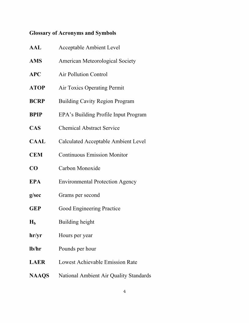
Glossary of Acronyms and Symbols AAL Acceptable Ambient Level AMS American Meteorological Society APC Air Pollution Control ATOP Air Toxics Operating Permit BCRP Building Cavity Region Program BPIP EPA’s Building Profile Input Program CAS Chemical Abstract Service CAAL Calculated Acceptable Ambient Level CEM Continuous Emission Monitor CO Carbon Monoxide EPA Environmental Protection Agency g/sec Grams per second GEP Good Engineering Practice Hb Building height hr/yr Hours per year lb/hr Pounds per hour LAER Lowest Achievable Emission Rate NAAQS National Ambient Air Quality Standards

5

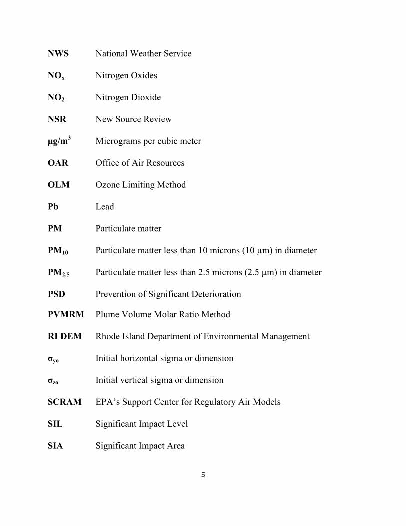
NWS National Weather Service NOx Nitrogen Oxides NO2 Nitrogen Dioxide NSR New Source Review μg/m3 Micrograms per cubic meter OAR Office of Air Resources OLM Ozone Limiting Method Pb Lead PM Particulate matter PM10 Particulate matter less than 10 microns (10 µm) in diameter PM2.5 Particulate matter less than 2.5 microns (2.5 µm) in diameter PSD Prevention of Significant Deterioration PVMRM Plume Volume Molar Ratio Method RI DEM Rhode Island Department of Environmental Management σyo Initial horizontal sigma or dimension σzo Initial vertical sigma or dimension SCRAM EPA’s Support Center for Regulatory Air Models SIL Significant Impact Level SIA Significant Impact Area

6

SO2 Sulfur Dioxide tpy tons per year USGS United States Geological Survey VOC Volatile Organic Compounds

7

Definitions Air contaminant: Soot, cinders, ashes, any dust, fumes, gas, mist, smoke, vapor, odor, toxic or radioactive material, particulate matter, or any combination of these. Albedo: The fraction of total incident solar radiation reflected by the surface back to space without absorption. Ambient air: The portion of the atmosphere to which the general public has access. Attainment or unclassifiable area: For any air pollutant, an area which is not designated as a nonattainment area. Background: Air contaminant concentrations present in the ambient air that are not attributed to the source(s) or facility(ies) being evaluated. Bowen ratio: An indicator of surface moisture, the ratio of sensible heat flux to latent heat flux. Together with albedo and other meteorological observations, this ratio is used for determining planetary boundary layer parameters for convective conditions driven by the surface sensible heat flux Criteria pollutant: A pollutant for which a national ambient air quality standard (NAAQS) has been defined. Digital Elevation Model (DEM): An array of elevations, usually at regularly spaced intervals, for a number of ground positions. Exceedance: In excess of a pre-established comparison level. Emission point: Point of constituent emissions release into the air. Facility or stationary source: All pollutant-emitting activities which belong to the same industrial grouping, are located on one or more contiguous or adjacent properties, and are under the control of the same person (or persons under common control). Pollutant-emitting activities shall be considered as part of the same industrial grouping if they belong to the same "major group" (i.e. which have the

8

same two-digit code) as described in the Standard Industrial Classification Manual, 1987. A facility or stationary source may consist of one or more emissions units. A facility or stationary source does not include emissions resulting directly from an internal combustion engine for transportation purposes, emissions from a nonroad engine or the activities of any vessel.

Isopleth: A line drawn on a map through all points having the same numerical value.

Model: A quantitative mathematical representation or simulation that uses building, stack, emissions and meteorological information to predict the impact of air contaminants emitted by one or more sources on ambient air.

National Ambient Air Quality Standards (NAAQS): Air quality standards set by the United States Environmental Protection Agency (EPA) to protect the public health and welfare. [40 CFR Part 50] National Elevation Dataset (NED): A seamless dataset with the best available raster elevation data of the conterminous United States, Alaska, Hawaii, and territorial islands. NED is the primary elevation data product of the USGS and is designed to provide National elevation data in a seamless form with a consistent datum, elevation unit, and projection. Data corrections were made in the NED assembly process to minimize artifacts, perform edge matching, and fill sliver areas of missing data. Nonattainment area: For any air pollutant, an area which is shown by monitored data or is calculated by air quality modeling based on monitored data to exceed any National Ambient Air Quality Standard for such pollutant and which has been designated as such in the Federal Register. North American Datum of 1927 (NAD27): Horizontal control datum for the United States defined with an initial point at Meads Ranch, Kansas, and by the parameters of the Clarke 1866 ellipsoid. The locations of features on USGS topographic maps, including the definition of 7.5-minute quadrangle corners, are referenced to the NAD27. North American Datum of 1983 (NAD83): An Earth-centered datum that uses the Geodetic Reference System 1980 (GRS 80) ellipsoid, unlike NAD27, which is based on an initial point (Meads Ranch, Kansas). Using recent measurements with

9

modern geodetic, gravimetric, astrodynamic, and astronomic instruments, the GRS 80 ellipsoid has been defined as a best fit to the worldwide geoid. Because the NAD83 surface deviates from the NAD27 surface, the position of a point based on the two reference datums will be different. Property: All land under common control or ownership coupled with all improvements on such land, and all fixed or movable objects on such land, or any vessel on the waters of this state. Receptor: A location where a person could be exposed to an air contaminant in the ambient air. Refined model: A model that provides a detailed treatment of physical and chemical atmospheric processes and requires detailed and precise input data. The outputs are more accurate than those obtained from conservative screening techniques. Screening technique: A conservative analysis technique to determine whether a given source is likely to pose a threat to air quality. Source: A point of origin of air contaminants, whether privately or publicly owned or operated. When used in the context of modeling, the term “source” refers to the emission point. Surface roughness length: A measure of the height of obstacles to the wind flow. This length is not equal to the physical dimensions of the obstacles, but is generally proportional to them. Universal Transverse Mercator projection (UTM): A widely used map projection that employs a series of identical projections around the world in the mid-latitude areas, each spanning six degrees of longitude and oriented to a meridian. This projection preserves angular relationships and scale and a rectangular grid can easily be superimposed on it. Many worldwide topographic and planimetric maps to scales ranging between 1:24,000 and 1:250,000 use this projection. World Geodetic System 1972 (WGS 72): The definition of Defense Mapping Agency (DMA) DEMs, as presently stored in the USGS database, references the

10

WGS 72 datum. WGS 72 is an Earth-centered datum. The WGS 72 was the result of an extensive effort extending over approximately three years to collect selected satellite, surface gravity, and astrogeodetic data available throughout 1972. These data were combined using a unified WGS solution (a large-scale least squares adjustment). World Geodetic System 1984 (WGS 84): The WGS 84 datum was developed as a replacement for WGS 72 by the military mapping community as a result of new and more accurate instrumentation and a more comprehensive control network of ground stations. The newly developed satellite radar altimeter was used to deduce geoid heights from oceanic regions between 70 degrees north and south latitude. Geoid heights were also deduced from ground-based Doppler and ground-based laser satellite-tracking data, as well as surface gravity data. This system is described in “World Geodetic System 1984,” DOD DMA TR8350.2 September 1987. New and more extensive data sets and improved software were used in the development.

11

1.0 INTRODUCTION The purpose of this guideline is to standardize the procedures used to conduct air dispersion modeling analyses submitted to the Rhode Island Department of Environmental Management (RI DEM) Office of Air Resources (OAR) to determine compliance with Rhode Island Air Pollution Control Regulation (RIAPCR) No. 22 Acceptable Ambient Levels (AALs) and with the National Ambient Air Quality Standards (NAAQS). A modeling protocol consistent with this guidance must be submitted to and be approved by the OAR prior to the submission of any modeling analysis unless the OAR agrees, in writing, that a modeling protocol is not necessary. Modeling protocols must include specific input data descriptions and include all of the information specified in Section 5.1 and Appendix B.

2.0 CRITERIA POLLUTANT OVERVIEW The US Environmental Protection Agency (EPA) has established NAAQS for a set of air contaminants commonly referred to as “criteria pollutants.” The criteria pollutants are: carbon monoxide (CO), sulfur dioxide (SO2), particulate matter (PM10 and PM2.5), nitrogen dioxide (NO2), ozone and lead. The NAAQS specify allowable ambient air concentrations for each criteria pollutant. Depending on the pollutant, standards are set for short-term (24-hours and less) and/or long-term (annual) exposure periods. Rhode Island implements these federal standards. The NAAQS for the criteria pollutants are available on the EPA website at (http://www.epa.gov/air/criteria.html) and are listed in Table A-1 of Appendix A. Modeling to demonstrate compliance with the NAAQS for CO, SO2, PM10, PM2.5, NO2, and lead is required in preconstruction permit applications, as specified in Section 2.1 below. In addition, EPA’s Prevention of Significant Deterioration (PSD) regulations, adopted in Section 9.5 of Rhode Island Air Pollution Control Regulation (RI APCR) No. 9, include additional criteria designed to limit degradation of air quality in areas that are currently in attainment of the NAAQS. Rhode Island is currently classified as an attainment or attainment/unclassifiable area for all criteria pollutants, although the designation for ozone may change in coming years, due to monitored violations of that NAAQS. Rhode Island is one of the northeast states in the Ozone Transport Region. As a result, nonattainment new

12

source review (Section 9.4 of RI APCR No. 9) applies to new major stationary sources or major modifications of VOC or NOx. Modeling of criteria pollutant emissions in conjunction with modifications to Rhode Island’s State Implementation Plan or in conjunction with preconstruction permit applications must be consistent with the procedures specified in the EPA Guideline on Air Quality Models (40 CFR 51, Appendix W). Note that, due to the complex nature of ozone formation, source-specific air dispersion modeling historically has not been required for that criteria pollutant. However, the EPA is currently reevaluating this issue and may modify Appendix W in the future to include methodology for source-specific ozone modeling.

2.1 Who Must Conduct Criteria Pollutant Air Dispersion Modeling? Applications for preconstruction permits for Rhode Island sources that meet any of the following criteria must include criteria pollutant air dispersion modeling analyses: 1. New major stationary sources, as defined in RI APCR No. 9, Subsection

9.5.1(f). These sources are subject to PSD air quality impact analysis requirements, as specified in Section 9.5 of that regulation.

2. New major stationary sources, as defined in RI APCR No. 9, Subsection

9.4.1(a) that are subject to the requirements of subsections 9.4.2(f) or (g). 3. Existing major stationary sources applying for a permit for a modification that

would increase potential emissions for one or more pollutant by an amount that exceeds the significant emissions rate thresholds listed in Table I below must conduct an air dispersion analysis for each pollutant that exceeds those thresholds. Such modifications are considered major modifications and are subject to the requirements specified in RI APCR No. 9, Sections 9.4 or 9.5, as applicable.

4. Applicants for minor source permits for new sources that have the potential to

emit one or more criteria pollutant in an amount that exceeds the significant emissions rate thresholds listed in Table I below must conduct an air dispersion analysis for each pollutant that exceeds those thresholds.

13

5. Applicants for minor source permits for existing sources if the modification results in an increased emission rate of any criteria pollutant that exceeds the significant emissions rate thresholds listed in Table I below must conduct an air dispersion analysis for each pollutant that exceeds those thresholds.

6. The OAR may request criteria pollutant modeling for other new or modified

sources if the OAR believes that emissions from such sources may cause or contribute to a violation of a NAAQS or a PSD increment or may pose a threat to public health or welfare. If a proposed increase in the hourly emission rate of a criteria pollutant is of sufficient magnitude that it may cause or contribute to a violation of a short-term ambient air quality standard or a PSD increment, modeling may be required even if the annual emissions increase does not exceed the significant emissions rate thresholds in Table I.

Table I - Significant Emissions Rate Thresholds

Air Contaminant Significant Emission Rate (tons/yr)Carbon monoxide (CO) 100 Nitrogen oxides (NOx) 25 Sulfur dioxide (SO2) 40

Particulate matter <10 µ (PM10) 15 Particulate matter <2.5 µ (PM2.5) 10

Lead (Pb) 0.6

2.2 Preliminary Modeling Analysis for Criteria Pollutants - Overview As a first step, sources may conduct a preliminary modeling analysis that evaluates only the emissions from the proposed new source or the net emissions increase associated with the proposed modification. Further modeling may not be required if the highest modeled concentration predicted by the preliminary analysis for each pollutant and averaging time is less than the corresponding significant impact level (SIL) listed in Table II. If the preliminary analysis predicts an exceedance of one or more SILs or if the OAR determines that the impacts associated with emissions from the source, in conjunction with impacts from other sources and background

14

concentrations, may result in an exceedances of a NAAQS, a refined multisource modeling analysis may be required, as discussed in Section 2.3.

Table II Significant Impact Levels (SILs)

Pollutant Significant Impact Levels

μg/m3 Particulate Matter (PM10) 24-hour 5 Particulate Matter (PM2.5) 24-hour 1.2 Annual 0.3 Sulfur Dioxide (SO2) 1-hour 7.8 24-hour 5 Annual 1 Carbon Monoxide (CO) 1-hour 2,000 8-hour 500 Nitrogen Dioxide (NO2) 1-hour 7.5 Annual 1

2.3 Refined Modeling Analysis for Criteria Pollutants - Overview If a preliminary analysis predicts an impact for one or more pollutant and averaging time that is above the corresponding SIL (a significant ambient impact), the project’s Significant Impact Area (SIA) must be calculated. The SIA is generally a circular area with a radius extending from the source to the most distant point where a significant ambient impact will occur, as predicted by the preliminary modeling or another approved dispersion modeling analysis. The SIA should be determined for each pollutant and averaging period for which a SIL is exceeded. Non-circular SIAs may be allowed on a case-by-case basis with prior approval from the OAR. If a preliminary analysis shows an exceedance of one or more SILs or if the OAR determines that the impacts associated with emissions from a subject source, in conjunction with impacts from interacting sources and background concentrations, may result in an exceedance of a NAAQS, a multisource modeling analysis, as specified in Section 5.7, may be required. Applicants preparing a criteria pollutant

15

modeling analysis should contact RI DEM to determine which interacting sources, if any, should be modeled in conjunction with the subject source. In determining whether multisource modeling is required, RI DEM will consider such factors as: the type and size of the subject source and potentially interacting sources, the SIA (calculated as discussed above), the distance between the subject source and a potentially interacting source, the concentration gradient in the vicinity of the subject source, monitored background concentrations and the likelihood of modeled violations of air quality standards. Multisource modeling also may be required for increment analyses. To determine whether a new or modified source causes or contributes to a violation of a NAAQS, monitored background concentrations are added to the following values, as determined by refined modeling that includes all sources of that pollutant associated with the subject facility as well as any interacting sources specified by the OAR:

• For the 1-hour and 8-hour CO NAAQS and the 3-hour and 24-hour SO2 NAAQS, the highest, second high modeled concentration for those averaging times for each of the 5 years modeled;

• For the annual average NO2 and SO2 NAAQS, the highest predicted annual

average concentration; • For the one-hour average NO2 NAAQS, the highest average of the 98th

percentile (8th highest) daily maximum one-hour concentrations at each receptor for each of the five years modeled;

• For the one-hour average SO2 NAAQS, the highest average of the 99th

percentile (4th highest) daily maximum one-hour concentrations at each receptor for each of the five years modeled.;

• For the 24-hour PM10

NAAQS, the 6th highest predicted concentration for the five years modeled (and, in general, when n years are modeled, the (n+1)th highest concentration over the n-year period));

• For the annual average PM2.5 NAAQS, the highest average of the modeled

annual averages at each receptor for the five modeled years;

16

• For the 24-hour average PM2.5 NAAQS, the highest average of the maximum modeled 24-hour averages at each receptor across the five modeled years; and

• For the lead NAAQS, the maximum 3-month rolling average in the five

year period at each receptor. As discussed above, a modeling analysis showing compliance with the ozone NAAQS is generally not required in conjunction with permit applications. Background ambient concentrations for facilities conducting air dispersion modeling to demonstrate compliance with NAAQS requirements are posted on the RI DEM website at www.dem.ri.gov/programs/benviron/air/pdf/dispdata.pdf. EPA guidance1 presents a three-tiered approach for demonstrating compliance with the 1-hour NO2 NAAQS. Tier 1 assumes that all NO emitted from a source is converted to NO2. Tier 2 uses the Ambient Ratio Method (ARM) to calculate the portion of NO that is converted to NO2. As recommended in a 2011 EPA guidance memo2, the OAR allows the use of a default ambient ratio of 0.80 without further justification. Tier 3 uses the Ozone Limiting Method (OLM) or Plume Volume Molar Ratio Method (PVMRM) to predict NO to NO2 conversion. Tier 3 methodology must be approved by the OAR prior to deployment. Hourly ambient ozone data, for use in conjunction with Tier 3 procedures, are posted on the RI DEM website at www.dem.ri.gov/programs/benviron/air/pdf/ozdata.xls. Note that the above techniques assume that the model is run with five years of off-site meteorological data. Alternatively, facilities may collect and utilize one year of on-site data. Applicants who plan to collect on-site meteorological data for use in modeling should meet with OAR prior to beginning data collection to discuss siting criteria, parameter selection, instrumentation, data processing, quality control measures and other factors relevant to collecting data that will be appropriate for modeling purposes.

1 USEPA, Memo from Stephen D. Page, Director, Office of Air Quality Planning and Standards, to Regional Air Division Directions, “Guidance Concerning the Implementation of the 1-hour NO2 NAAQS for the Prevention of Significant Deterioration Program, June 29, 2010. 2 USEPA, Memo from Tyler Fox, Air Quality Modeling Group to Regional Air Division Directions, “Additional Clarification Regarding Application of Appendix W Modeling Guidance for the 1-hour NO2 National Air Quality Standard, Mar. 1, 2011.

17

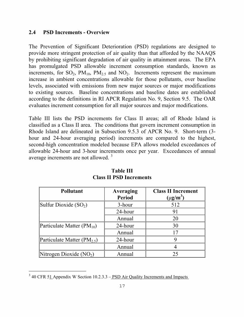
2.4 PSD Increments - Overview The Prevention of Significant Deterioration (PSD) regulations are designed to provide more stringent protection of air quality than that afforded by the NAAQS by prohibiting significant degradation of air quality in attainment areas. The EPA has promulgated PSD allowable increment consumption standards, known as increments, for SO2, PM10, PM2.5 and NO2. Increments represent the maximum increase in ambient concentrations allowable for those pollutants, over baseline levels, associated with emissions from new major sources or major modifications to existing sources. Baseline concentrations and baseline dates are established according to the definitions in RI APCR Regulation No. 9, Section 9.5. The OAR evaluates increment consumption for all major sources and major modifications. Table III lists the PSD increments for Class II areas; all of Rhode Island is classified as a Class II area. The conditions that govern increment consumption in Rhode Island are delineated in Subsection 9.5.3 of APCR No. 9. Short-term (3-hour and 24-hour averaging period) increments are compared to the highest, second-high concentration modeled because EPA allows modeled exceedances of allowable 24-hour and 3-hour increments once per year. Exceedances of annual average increments are not allowed. 3

Table III

Class II PSD Increments

Pollutant Averaging Period

Class II Increment (μg/m3)

Sulfur Dioxide (SO2) 3-hour 512 24-hour 91 Annual 20 Particulate Matter (PM10) 24-hour 30 Annual 17 Particulate Matter (PM2.5) 24-hour 9 Annual 4 Nitrogen Dioxide (NO2) Annual 25

3 40 CFR 51 Appendix W Section 10.2.3.3 – PSD Air Quality Increments and Impacts

18

3.0 AIR TOXICS MODELING OVERVIEW For a facility to obtain an air toxics operating permit (ATOP), Subsection 22.5.3 of RI APCR No. 22 requires a demonstration that emissions from the facility do not cause ground-level impacts of any toxic air contaminant in exceedance of the Acceptable Ambient Levels (AALs) listed in that regulation. New sources must make a similar demonstration for both listed and non-listed air toxics in order to obtain a preconstruction permit. The OAR develops Calculated Acceptable Ambient Levels (CAALs) for evaluating impacts of non-listed air toxics from new sources in conjunction with preconstruction permit applications, as needed. Since the AALs and CAALs refer to the increase in concentration of a pollutant associated with emissions from a local facility, background concentrations of the pollutant are not considered when evaluating compliance with those standards.

4.0 COMPLIANCE DEMONSTRATION OVERVIEW– CRITERIA POLLUTANTS AND AIR TOXICS Dispersion modeling for comparison to SILs, NAAQS, PSD increments, AALs and CAALs must use the AERSCREEN and/or AERMOD air dispersion models. Information about emissions; stacks; building orientation and dimensions; topographic coordinate locations; meteorology; background concentrations; and surface characteristics such as Bowen ratio, Albedo, and surface roughness are input into these models, which then mathematically simulate the dispersion of the pollutant and estimate the ambient concentration of that pollutant which would occur as a result of those emissions at various distances from the source. This guideline specifies allowable modeling procedures for both air toxics and criteria pollutants, but cannot anticipate every potential situation. Screening level modeling for air toxics operating permits may be performed by OAR staff using the AERSCREEN model. In lieu of accepting emissions limits based on screening modeling results, a facility may choose to perform or to hire a contractor to perform a refined modeling analysis using AERMOD. Modeling required for permits for new or modified sources must be submitted with the preconstruction permits for those projects.

19

When modeling is to be performed by a facility or its contractor, the applicant must submit a modeling protocol to the Office of Air Resources before undertaking the modeling analysis unless the OAR agrees, in writing, that a modeling protocol is not necessary. General guidance on dispersion modeling is found in 40 CFR 51, Appendix W (EPA’s Guideline on Air Quality Models) and the models discussed in this document, along with the accompanying User’s Guides, are available on the EPA’s Support Center for Regulatory Air Models (SCRAM) website, http://www.epa.gov/scram001. This guideline presents an approach to air modeling which begins with the collection of basic source information. The modeler then calculates Good Engineering Practice (GEP) stack height, performs a building cavity analysis, and uses a screening model to predict downwind impacts. Screening models, like AERSCREEN, are designed to produce conservative (i.e. biased high) ambient concentration estimates by using worst case meteorology. In many cases, a screening analysis provides an adequate demonstration of compliance with applicable standards. If such a demonstration cannot be made using screening modeling procedures, then a refined analysis using actual hourly meteorological data is necessary. The 2013 revisions to this guideline are effective immediately. Screening modeling in connection with any permit application or air toxics operating permit renewal application submitted or due to be submitted on or after 15 June 2011 must use the AERSCREEN model. Refined modeling in connection with any application submitted or due to be submitted on or after 1 January 2006 must use AERMOD, as specified in Section 5.0.

5.0 REQUIREMENTS FOR AIR QUALITY ANALYSIS - OVERVIEW Section 5 provides an overview of the components of a modeling study. Details regarding modeling techniques are discussed in the sections that follow. On November 9, 2005 the EPA published a Federal Register notice revising its Guideline on Air Quality Models (40 CFR 51, Appendix W) to recommend the use of the AERMOD pollution dispersion model as the primary tool for refined modeling to predict air quality impacts for permitting purposes. On March 3, 2011, EPA released a non-beta version of AERSCREEN, which replaced

20

SCREEN3 and is now required in Rhode Island for all screening level air dispersion analyses.

5.1 Modeling Protocol As discussed above, a modeling protocol must be submitted to and approved by the OAR prior to the submission of modeling to demonstrate compliance with Rhode Island and Federal standards, unless the OAR agrees, in writing, that a modeling protocol is not necessary. The protocol must document in detail how the applicant proposes to conduct the modeling analysis and how the results will be presented. Those procedures must be consistent with the specifications in this document. In general, a modeling protocol should contain the following information: • Project description, including a project overview, facility plot plan, and

emissions and stack parameters;

• Proposed project parameters, including a land use analysis, description of the local topography, a Good Engineering Practice (GEP) stack height analysis, local anemometer height and the meteorological data proposed for use in the modeling analysis;

• A list of the Federal and Rhode Island air standards that apply to the proposed

project; • Proposed air quality analysis techniques, including model selection, screening

analysis methods, and proposed methods for refined modeling. • Special modeling considerations, including the approach for addressing effects

of coastal fumigation, health risk assessment, fugitive emissions, deposition and odor modeling, if necessary;

Background air quality monitoring data to be used in criteria pollutant impact analyses. Note that background criteria pollutant levels are available on the RI DEM website at: www.dem.ri.gov/programs/benviron/air/pdf/dispdata.pdf.

21

• If multisource modeling is required, as specified in Section 5.7, the methods used to determine the significant impact area (SIA) and to generate the list of sources to be modeled and relevant information about those sources;

• An identification of the meteorological data that will be used in the modeling

analysis. Note that the most recent five years of preprocessed meteorological data for the NWS surface station ID No. 14765 (TF Green Airport) and NWS upper air station ID No. 14684 (Chatham, MA), including 1-minute ASOS wind .DAT data files and .SFC and .PFL data files, are available from the OAR or on the RI DEM website at www.dem.ri.gov/programs/benviron/air/pdf/metdata.zip. Onsite or other alternative meteorological data sets will be accepted if they are technically justified. Descriptions of alternative data must include the location of meteorological towers and specific information about the wind and temperature data, as well as how the surface characteristics were obtained; and

• The form of presentation of air quality modeling results, including the way that

significant impact areas and compliance demonstrations will be presented. Appendix B of this document contains a summary checklist that can be used to aid in assessing the completeness of an air quality modeling protocol and analysis. It is strongly recommended that this checklist be reviewed by the applicant before any documents are submitted to the OAR. Modeling protocols and analyses should be sent to: RI Department of Environmental Management Office of Air Resources 235 Promenade Street Providence, RI 02908-5767

5.2 Facility Data The use of accurate and complete facility data is essential for obtaining accurate modeling results. The following information is required for most air dispersion modeling demonstrations:

22

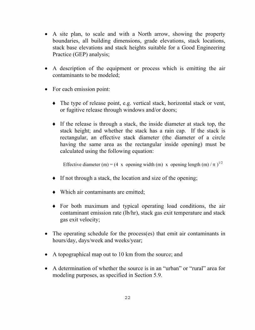
• A site plan, to scale and with a North arrow, showing the property boundaries, all building dimensions, grade elevations, stack locations, stack base elevations and stack heights suitable for a Good Engineering Practice (GEP) analysis;

• A description of the equipment or process which is emitting the air

contaminants to be modeled;

• For each emission point:

♦ The type of release point, e.g. vertical stack, horizontal stack or vent, or fugitive release through windows and/or doors;

♦ If the release is through a stack, the inside diameter at stack top, the

stack height; and whether the stack has a rain cap. If the stack is rectangular, an effective stack diameter (the diameter of a circle having the same area as the rectangular inside opening) must be calculated using the following equation:

Effective diameter (m) = (4 x opening width (m) x opening length (m) / π )1/2

♦ If not through a stack, the location and size of the opening;

♦ Which air contaminants are emitted;

♦ For both maximum and typical operating load conditions, the air

contaminant emission rate (lb/hr), stack gas exit temperature and stack gas exit velocity;

• The operating schedule for the process(es) that emit air contaminants in

hours/day, days/week and weeks/year;

• A topographical map out to 10 km from the source; and

• A determination of whether the source is in an “urban” or “rural” area for modeling purposes, as specified in Section 5.9.

23

All emission points under review should be modeled at both maximum and typical operating load conditions. If compliance with regulatory limits can be demonstrated at typical operating load conditions but not at maximum load conditions, load restrictions may be stipulated in permits.

5.3 GEP Analysis A GEP stack height analysis must be conducted in accordance with the EPA stack height regulation (40 CFR 51.118) and the Guideline for Determination of Good Engineering Practice Stack Height (USEPA, 1985). The formula for the GEP stack height, as defined by the EPA guidelines, is as follows:

HGEP

= Hb + 1.5 L

where: H

GEP is formula GEP stack height,

Hb is the height of adjacent or nearby building,

L is the lesser of the height and the maximum projected width of adjacent or nearby building, i.e., the critical dimension.

A stack is considered close enough to a building to be affected by downwash if it is located within the lesser of 0.8 kilometer or 5L of the building in any wind direction. For sources that are near more than one building or buildings with multiple roof heights, the building with the greatest GEP height is said to be the “controlling building” or “controlling tier” and is the one used in screening modeling. For refined modeling, a more detailed GEP analysis is required in which the controlling building (its height and width perpendicular to the wind) are identified for 36 different wind directions, starting with North and spaced 10o azimuth around the compass The GEP stack height analysis must identify all buildings on and off-site with the potential to cause aerodynamic downwash of emissions from the stack. This analysis need only consider buildings within the lesser of 0.8 kilometer or 5 L of the stack. For each stack, a table shall be provided with the following data for each building (or tier):

24

a. Building height (relative to stack base elevation); b. Maximum projected building width; c. Distance from the stack; d. 5L distance; and e. Formula GEP stack height, calculated as specified above. The table should identify the building associated with the greatest formula GEP stack height. In addition to the GEP stack height table, a table must be provided that lists coordinates for all stacks and for each corner of any structure (or structure tiers) that are within 5L of the stack. The EPA's Building Profile Input Program with the Plume Rise Model Enhancements (BPIPPRM) is used to derive the parameters necessary to simulate directional dependent aerodynamic downwash in the model and should be run for all sources that will be modeled with AERMOD. The output from BPIPPRM is used by AERMOD to calculate downwash from all stacks. A paper copy of the output from this program can be used as a substitute for the table listing coordinates of stacks and corners of structures discussed above. Input/output files from the BPIPPRM program should be submitted to the OAR in electronic format with the protocol. The analysis of proposed or modified sources may not employ dispersion techniques (as defined in 40 CFR 51.100(hh)) or seek to increase the height of an existing stack unless the provisions in 40 CFR 51.100(kk)2 are met. If the height of the stack is above both the calculated formula GEP height and the de minimus GEP height of 65 meters, the higher of either the calculated GEP height or 65 meters (not the actual stack height ) must be used in the modeling to demonstrate compliance with standards.

5.4 Requirements for Cavity Analysis AERSCREEN and AERMOD incorporate the Plume Rise Model Enhancements (PRIME) (Schulman et al. 2000) algorithms for estimating enhanced plume growth and restricted plume rise for plumes affected by building wakes (US EPA 1995). PRIME partitions plume mass between a cavity recirculation region and a dispersion enhanced wake region based upon the fraction of plume mass that is calculated to intercept the cavity boundaries, regardless of GEP stack height. Concentrations in cavities can be relatively high, due to the limited air volume into which air contaminants are mixed The objectives of a cavity analysis are: (1) to

25

determine if the cavity extends beyond a facility's property line with any wind direction, and, if so, then (2) to determine if the maximum concentrations in the cavity exceed any standard for all applicable averaging periods. Guidance on cavity modeling techniques is given in Section 6. Compliance with applicable standards in the cavity analysis does not eliminate the need to do dispersion modeling for areas outside of the downwash cavity.

5.5 Screening Modeling Overview - Wake Region Screening modeling is a procedure used to conservatively calculate air contaminant concentrations outside cavity regions (in the wake region) at receptors on and beyond a facility's property line. If predicted concentrations are less than the applicable standards for those air contaminants, no further analysis is required. Note that, for criteria pollutant modeling, background concentrations must be added to predicted maximum predicted impacts for each applicable pollutant and averaging time for comparison with the NAAQS. Since the AALs for air toxics in RI APCR No. 22 do not consider background concentrations, modeled impacts for those pollutants are compared directly with the AALs. In addition, note that criteria pollutant modeling for comparison to SILs does not include the consideration of background concentrations. If predicted impacts exceed an applicable standard by a factor of less than 10, refined modeling techniques, which generally reduce estimated impacts, may be used. If the impacts predicted by screening modeling exceed an applicable standard by a factor of 10 or more, it is very unlikely that refined modeling would demonstrate compliance, and the facility may wish to investigate techniques for reducing emissions or improving dispersion characteristics before additional modeling is undertaken. Screening modeling must consider receptors in both simple and complex terrain, the latter being elevations above stack top. Guidance on screening modeling techniques for wake regions is given in Section 7 of this document.

5.6 Refined Modeling Overview - Wake Region A refined model provides a detailed analysis of the process of transport and dispersion of emissions from one or multiple sources and predicts impacts from

26

those emissions at a large numbers of receptor points downwind. Refined modeling requires either one year of hourly meteorological data collected on-site or the latest five full years of hourly data from a representative National Weather Service (NWS) site. If there is a violation of an applicable standard the source will need to reduce predicted impacts, e.g. by reducing emissions through process modifications or by changing stack parameters before a permit is issued. Refined modeling must consider receptors in both simple and complex terrain. Guidance on refined modeling techniques is given in Section 8.

5.7 Multisource Modeling Analysis As discussed in Section 2.3, applicants preparing a criteria pollutant modeling analysis should contact RI DEM to determine which interacting sources, if any, need to be modeled in conjunction with the subject source. Multisource modeling also may be required for increment analyses. Modeling input data for interacting sources will be provided to the applicant by RI DEM if available. Applicants should submit an inventory to RI DEM prior to conducting multisource modeling which lists the sources that will be included in the analysis and the critical parameters needed to model those sources, including the emission units, emission rates, and stack parameters for each source that will be included in the modeling analysis. Building parameters must also be included if downwash effects are important for accurately predicting a source’s contribution to the multisource impact. For a proposed source or modification with a SIA that approaches or extends into an adjacent state, a similar type of inventory must be obtained from that state as well. In cases where a large number of nearby sources have been identified, the applicant may propose screening techniques to limit the number of sources that are explicitly modeled. The modeling protocol should discuss the screening methodology used to eliminate sources and the results of this analysis. The applicant should obtain the OAR’s agreement on the methodology selected to include and remove sources from the inventory before submittal of the multisource inventory.

5.8 Modeling to Determine Maximum Allowable Emissions for Air Toxics

27

In addition to determining compliance with applicable standards, modeling can be used to calculate the maximum emissions rate of an air contaminant allowed for a facility. For air toxics, if the air contaminant is emitted from only one source at the facility, the maximum allowable emissions rates are calculated according to the following formulas: Max Allowable Emissions (lb/hr) = [1-hr AAL (μg/m3) / Max Modeled 1- hr Impact

(μg/m3)] * Modeled Emissions Rate (g/sec) * 7.94 lb/hr / g/sec

Max Allowable Emissions. (lb/dy) = [24-hr AAL (μg/m3) / Max Modeled 24- hr

Impact (μg/m3)] * Modeled Emissions Rate (g/sec) * 7.94 lb/hr / g/sec * 24 hr/dy

Max Allowable Emissions (lb/yr) = [annual AAL (μg/m3) / Max Modeled Annual

Impact (μg/m3)] * Modeled Emissions Rate (g/sec) * 7.94 lb/hr / g/sec * 8760 hr/yr

If more than one source at the facility emits the air contaminant, the dispersion characteristics of the sources may not be equivalent, and this fact must be considered when calculating maximum allowable emissions rates. Since the determination of compliance with NAAQS generally requires the addition of background concentrations to predicted impacts, the above equations do not apply to those determinations. To calculate the most accurate maximum emissions rate, refined modeling, rather than screening modeling, should be used for the non-cavity region. However, refined modeling is not necessary when the maximum ground-level concentration in the cavity region is greater than the value predicted in the non-cavity region using screening modeling or if the facility is willing to limit its emissions to the maximum allowable emission rate calculated using the screening modeling results.

5.9 Land Use Considerations Section 7.2.3 of the Guideline on Air Quality Models (EPA, 2005) provides the basis for determining the urban/rural status of a source. For most applications the

28

Land Use Procedure described in Section 7.2.3(c) is sufficient for determining the urban/rural status. That Guideline recommends that this determination be based on either land use or population density within a 3 km radius of the source. However, since the maximum impacts for many air emissions sources occur relatively close to the sources, a review of the area immediately surrounding a facility is most important. To perform the land use procedure: (1) classify the land use within the total area circumscribed by a 3 km radius circle about the source using the meteorological land use typing scheme shown in Table IV (Auer, 1978) (2) if land use Types I1, I2, C1, R2, and R3 account for 50 percent or more of the total area, use urban dispersion coefficients; otherwise, use appropriate rural dispersion coefficients. Major roadways and clover leafs should be identified as urban land use areas. Unless the source is located in an area that is distinctly urban or rural, the land use analysis should provide the percentage of each land use type from the Auer scheme and the total percentages for urban versus rural. The latest available United States Geological Survey (USGS) topographic quadrangle maps in the vicinity of the facility should be used in this analysis. Internet-based virtual globe maps and geographical information programs may also be used. In some circumstances, such as in an area undergoing rapid development, county or local planning board maps may need to be used.

Table IV Identification and Classification of Land Use

Type Use and Structures Vegetation

I1 Heavy Industrial: Major chemical, steel and fabrication industries; generally 3-5 story buildings, flat roofs

Grass and tree growth extremely rare; < 5% vegetation

I2 Light-moderate industrial: Rail yards, truck depots, warehouses, industrial parks, minor fabrications; generally 1-3 story buildings, flat roofs

Very limited grass, trees almost total absent; <5% vegetation

C1 Commercial: Office and apartment buildings, hotels; > 10 story heights, flat roofs

Limited grass and trees; < 15% vegetation

29

Type Use and Structures Vegetation R1 Common residential:

Single family dwelling with normal easements; generally one story, pitched roof structures; frequent driveways

Abundant grass lawns and light-moderately wooded; > 70% vegetation

R2 Compact residential: Single, some multiple, family dwelling with close spacing; generally < 2 story, pitched roof structures; garages (via alley), no driveways

Limited lawn sizes and shade trees; < 30% vegetation

R3 Compact residential: Old multi-family dwellings with close (<2 m) lateral separation; generally 2 story, flat roof structures; garages (via alley) and ash pits, no driveways

Limited lawn sizes, old established shade trees: < 35% vegetation

R4 Estate residential: Expansive family dwelling on multi-acre tracts

Abundant grass lawns and lightly wooded; > 95% vegetation

A1 Metropolitan natural: Major municipal, state, or federal parks, golf courses, cemeteries, campuses, occasional single story structures

Nearly total grass and lightly wooded; > 95% vegetation

A2 Agricultural rural Local crops (e.g., corn, soybean); > 95% vegetation

A3 Undeveloped: Uncultivated; wasteland

Mostly wild grasses and weeds, lightly wooded; > 90% vegetation

A4 Undeveloped rural Heavily wooded; > 95% vegetation

A5 Water surfaces: Rivers, lakes

RI APCR No. 22 allows the OAR to exempt impacts in areas that are not accessible to the public from consideration when determining compliance with AALs and CAALs. In addition, the OAR may, at its discretion, adjust annual or

30

24-hour AALs used to evaluate the impacts in areas where, due to land-use considerations, public exposure potential is limited. For example, exposures in industrially zoned areas are generally limited to 40 hours per week, as compared to the potential for continuous exposures in residential areas. A facility that wishes to exclude an area from a modeling analysis or to apply a less stringent AAL to an area where exposure opportunities are limited should supply documentation to the OAR that demonstrates land use restrictions in those areas.

6.0 BUILDING CAVITY MODELING TECHNIQUES AERSCREEN and AERMOD contain the PRIME downwash algorithm and therefore can calculate impacts in the cavity and near-wake regions of structures. A receptor spacing of no more than 10 meters is recommended in the immediate vicinity of the stacks and nearby buildings. A grid spacing of 25 meters is recommended for distances out to approximately 1 km in all directions from the source. Short stacks and vents on the sides and roofs of buildings can cause relatively high concentrations in the recirculation cavity behind a building. The length of this cavity is measured from the lee side of the building. As a first cut, the “include downwash” option in the latest version of EPA’s AERSCREEN model should be used to evaluate air contaminant impacts in the cavity region. AERSCREEN is available for download on the EPA’s SCRAM website. The first task is to identify which, if any, of the building cavities extend beyond a facility's property line and which, if any, stacks contribute to air contaminant concentrations in these cavities. Emissions from a stack should be assumed to be caught in a building’s cavity region if the stack is attached to the building under evaluation or is less than 2 Lb upwind of the building (where Lb is the smaller of the building height and width), 1/2 Lb from the sides of the building, or within LR (the recirculation cavity length) downwind. LR is calculated by the “include downwash” option of AERSCREEN. Emissions from horizontal stacks, vents that are essentially flush with the roof or sides of a building, doors and windows and other fugitive sources should always be assumed to be captured in the building cavity. Estimating the cavity lengths for four wind directions, each normal to one of the building faces, is generally sufficient for determining if any cavity regions extend

31

off-site. However, off-axis cavity regions may also have to be considered, depending on the shape of the property. Direction-specific building dimensions must be used to determine the extent of off-axis cavity regions. The Office of Air Resources has developed a computer program called BCRP (Building Cavity Region Program) that performs this task. This program displays building cavity regions and their relationship to facility property boundaries for thirty-six wind directions and can be used to determine if a cavity analysis is necessary. The BCRP program and user's guide can be obtained free of charge from the OAR. Building cavity models assume a simple block-like building. For buildings that are not square, a four-sided footprint of the building should be used for the cavity analysis. Emissions from a non-vertical stack, a vent or another fugitive source can be modeled with the AERSCREEN model as a point source with an exit velocity of 0.001 m/s with the flow rate held constant. This procedure eliminates plume rise from momentum. When there are multiple buildings or building tiers or multiple sources, the modeler must identify all sources that add air contaminant mass to the cavity region of each building or tier. In the case of a multi-tiered building, one approach is to use a simple block structure that simulates the general shape of the building complex. Another approach is to model each building tier separately and determine which tier causes the greatest impact. Modelers using that approach should be aware that modeling a single tall narrow tier without considering short wider tiers could produce unreasonable concentration results. In general, the impacts from individual building cavities should be modeled separately and the greatest predicted impact used to determine compliance. If cavity impacts for different sources of the same air contaminant at a facility overlap, then the predicted concentrations of that contaminant should be summed to determine impacts in the overlapping regions. For the case of multiple stacks in the same building cavity emitting the same air contaminant, each stack should be modeled separately and the results summed to obtain a total cavity concentration. Predicted concentrations in cavity regions that extend beyond the facility’s property line should be compared to applicable standards. Since AERSCREEN predicts one-hour, 3-hour, 8-hour, 24-hour, and annual impacts, no time-scaling adjustment of predicted impacts is necessary for comparison of impacts to standards with various averaging times. To simplify the analysis for situations

32

which involve more than one stack or building, the maximum AERSCREEN model impact output for a particular averaging period for an air contaminant in all applicable cavity regions can be summed and the sum compared to the applicable standard. Note that, for criteria air pollutants, the background concentration must be added to the predicted impacts before comparison with the NAAQS. If a facility cannot demonstrate compliance with the applicable standards in the cavity regions using AERSCREEN, refined cavity modeling can be conducted using the AERMOD refined dispersion model. This model is discussed further in Section 8 of this document. This option may also be chosen initially instead of AERSCEEN, particularly if refined modeling is necessary for the wake region or if multiple sources and/or buildings are involved in the analysis.

7.0 SCREENING MODELING TECHNIQUES– WAKE REGION The EPA’s AERSCREEN model should be used for screening level modeling of point (vertical uncapped stack), capped stack, horizontal stack, rectangular area, circular area, flare, and volume sources to calculate impact concentrations at receptors in simple terrain (elevations below stack top) and complex terrain. AERSCREEN data can be found on the RIDEM website: www.dem.ri.gov/programs/benviron/air/pdf/aerscreen.zip.

7.1 Time Scaling Factors AERSCREEN automatically scales one-hour impact predictions to provide 3-hour, 8-hour, 24-hour, and annual average time periods. Scaling factors currently utilized in AERSCREEN are as follows:

Averaging period Scaling Factors in AERSCREEN 3 hours 1.0 8 hours 0.9 24 hours 0.6 Annual 0.1

7.2 Receptor Locations – Screening Modeling

33

The receptor network must capture and adequately define the area of maximum impact. Discrete receptors and either a polar or Cartesian receptor grid network should be used. Polar grids generally contain 36 radii spaced at 10-degree intervals. A set of receptors should also be placed along the facility’s property line or fence line with a maximum interval of 10 to 20 meters. Where appropriate, receptors should be placed at sensitive locations such as schools, playgrounds, hospitals, and senior housing developments to insure that standards are not exceeded at these locations. A discrete receptor should be placed at the point on the property boundary that is closest to the source. AERSCREEN creates an automated distance receptor network grid including the minimum ambient distance, automatically calculating distances and any discrete receptor distances as described below:

• Spacing of 25 m from zero to 5 km • From 5 km to the final probe distance, the spacing is the greater of 25 m or a

spacing calculated by: (probe distance – 5,000 m)/100 where 100 represents 100 receptors

Once a maximum impact is found, additional receptors at 10 meter spacing around this point should be analyzed. The terrain height for each receptor is obtained from Digital Elevation Model (DEM) or National Elevation Dataset (NED) data files. A set of concentric circles should be drawn on the maps corresponding to the receptor distances from the source. The single terrain height for each receptor should be selected as the highest terrain that occurs anywhere in the annulus defined by:

• The circle in which the receptor is located and the next larger concentric circle and

• The two radii connecting the center of the concentric circles with the points

halfway between the receptor and the receptors on both sides of the receptor. By this method, every point on the map is examined in assigning maximum terrain heights to the receptors. If the initial screening runs show an exceedance of an AAL, CAAL, or, when added to the background concentration, a NAAQS, the

34

model can be run again with a more refined grid using actual receptor elevations in the vicinity of the point where the exceedance occurred. AERSCREEN provides the option for incorporating terrain impacts into the screening analysis. The user must create a file called demlist.txt. The first line of this file describes the type of terrain file being used. The file type must be DEM or NED. AERSCREEN interfaces with AERMAP (U.S. EPA, 2004b) to automate the processing of terrain information for simple elevated terrain and interfaces with AERMOD to perform the modeling runs. AERMAP requires either DEM or NED data in order to process the terrain. Simple terrain is land that is above stack base elevation but not higher than stack top. In AERSCREEN, flat and elevated (simple) terrain can be modeled at the same time. For simple terrain, AERSCREEN prompts the user to choose whether to include terrain processing (yes=include terrain, no=do not include terrain effects) as well as for source coordinates. If flat terrain is being processed for any source type, the user is not prompted to enter any terrain information and the function for AERMAP source elevation determination is not interfaced.

7.3 Screening Modeling Techniques for Point Sources AERSCREEN can be used for a single point, capped stack, or horizontal stack. Although the AERSCREEN model is only designed for single sources, the impacts from two or more point sources can be conservatively estimated by modeling each singly and then adding the maximum concentrations together, regardless of the associated downwind distances. This is a useful approach when individual impacts are small and compliance with regulatory standards can be easily demonstrated without using a refined model. The emissions from multiple stacks which are located within 100 meters of each other and which have volumetric flow rates that differ by no more than 20% can also be merged using the following procedure (EPA, Screening Procedures for Estimating the Air Quality Impact of Stationary Sources-Revised, EPA-450/R-92-019):

35

Step 1 Compute the parameter M for each stack to be merged where: M = (hs*V*Ts)/Q Where, M = merged stack parameter hs = stack height above ground (m) V = volumetric flow rate (π/4) ds

2 vs, (m3/s) ds = effective stack exit inside diameter, (m) vs = stack gas exit velocity, (m/s) Ts = stack gas exit temperature, (oK) Q = air contaminant emission rate, (g/s) Step 2. Determine which of the stacks has the lowest value of M. This is the representative stack. Step 3. Sum the emissions rates (Q) for the stacks that are being merged. This summed emission rate, along with the stack parameters for the representative stack. should be used in modeling the merged stacks. When modeling horizontal stacks or vertical stacks with rain caps, the exit velocity should be set to 0.001 m/s to eliminate plume rise from momentum and the flow rate should be held constant. In order to maintain a constant flow rate for vertical rain-capped stacks, the modeled stack diameter must be different from the actual stack diameter. The modeled stack diameter for vertical rain-capped stacks should be calculated using the following equation:

dm = da (Va/Vm)1/2

where: dm = modeled stack diameter; da = actual stack diameter; Vm = modeled stack exit velocity, i.e., 0.001 m/s; and Va = actual stack exit velocity.

If building downwash is to be considered, no stack tip downwash correction is made by the model. When building downwash is not to be considered, however, the model does make a stack tip downwash correction and the modeled stack diameter should be set equal to the actual stack diameter in order to avoid unrealistically small modeled stack heights. For horizontal stacks, the modeled stack diameter should be set equal to 1.0 meters.

36

7.4 Screening Modeling Techniques for Flare Sources Flares, such as those used to burn landfill gas, are modeled as flare sources in AERSCREEN. The technique to calculate buoyancy flux for flares generally follows the technique described in the AERSCREEN Model User’s Guide, which is available on the SCRAM website. The following parameters should be used when modeling flares:

• Emission rate (g/s) • Flare stack height (m) • Total heat release rate (cal/s) • Receptor height above ground (m) • Urban/rural option (U = urban, R = rural)

AERSCREEN processes flares as point sources. AERSCREEN defaults the exit velocity to 20 m/s and the exit temperature to 1,273o K.

7.5 Screening Modeling Techniques for Volume Sources The AERSCREEN model should also be used for the screening analysis of the non-cavity impacts of emissions from vents, along the faces and roofs of buildings, through doors and windows and in similar situations. These releases are best represented by a volume source having the dimensions of the building from which the emissions originate. Very short vertical stacks on buildings, those for which the stack height to building height ratio is below 1.2, can also be modeled as volume sources for receptors beyond the cavity region. Volume sources must have a square base, but need not be a cube. For a square, or nearly square, source the actual building dimensions (height and width) should be used for the screening analysis. For non-square sources, the width of the source should be set equal to the minimum building length. A volume source is defined by its release height (HS) and initial lateral and vertical dimensions, σyo and σzo respectively. The release height is the center of the volume

37

source and so it should be set equal to one-half the average building height. The initial lateral dimension for a volume source should be set equal to its width divided by 4.3. The initial vertical dimension for a volume source should be set equal to the average building height divided by 2.15. The location and elevation of receptors should be determined for volume sources in the same manner as for point sources. The downwind distance used in the model is measured from the center of volume source, not its edge. The modeler should be careful in measuring the distance to the first receptor.

7.6 Screening Modeling Techniques for Area Sources The AERSCREEN model should be used for a screening analysis of the impact of emissions from area sources such as landfills, surface impoundments, wastewater lagoons, tank farms, and other chemical storage areas. The release height should be set to zero, except in the case of tank farms and storage areas, where the release height should be set to the average height of the chemical release. AERSCREEN automatically calculates the emission rate per unit area to input into AERMOD. The downwind distance used in the model is measured from the center of the area source, not its edge. The modeler should be careful to measure the correct distance from the center of the area source to the nearest property line in setting the first receptor distance. Generally the receptor distance should not be less than the length of one side of the area source.

7.7 Screening Modeling Techniques for Facilities with Combinations of Point, Area, and Volume Sources The AERSCREEN model should be used for the screening analysis of the impact of emissions from facilities having combinations of point, area, and volume sources. All sources should be collocated and the impacts at each receptor due to each source should be summed. The modeler should remember that receptor distances are measured from the center of volume and area sources, not from the edge. If sources would not be realistically collocated, refined modeling may be more appropriate.

38

7.8 Complex Terrain Modeling – Screening Techniques AERSCREEN predicts impacts for a single source in both simple and complex terrain. AERSCREEN interfaces with AERMAP (U.S. EPA, 2004b) and BPIPPRM (Schulman et al. 2000; U.S. EPA, 2004d) to automate the processing of simple elevated, flat, complex terrain, and building information.

8.0 REFINED MODELING TECHNIQUES The AMS/EPA Regulatory model with the PRIME downwash algorithm (AERMOD) must be used for refined modeling of air toxics and criteria pollutant releases from any combination of point, area, and volume sources. AERMOD is required as the primary method for determining compliance with SILs, NAAQS, Class II PSD Increments and RI AALs and CAALs. Either one year of on-site meteorological data or the most recent five years of meteorological data from a representative NWS site must be used in the model. Facilities that plan to collect on-site meteorological data for use in a modeling study should meet with OAR prior to beginning data collection to discuss siting criteria, parameter selection, instrumentation, data processing, quality control measures and other factors relevant to collecting data that will be appropriate for modeling purposes. On-site meteorological data must be submitted with the modeling report in a current electronic format, along with a description of the procedures used to collect and process those data (e.g. monitor location, instrumentation, quality control, data processing). If on-site data are not used, the applicant should use the most recent five years of data available for NWS surface station ID No. 14765 (TF Green Airport) and NWS upper air station ID No. 14684 (Chatham, MA). Those data are available from the OAR free of charge. Use of alternative meteorological data sets is allowed only with prior OAR approval. Applicants must submit the 5-year meteorological datasets generated by AERMINUTE and AERMET with the modeling report. Refined modeling should be attempted only by people who are well trained in dispersion modeling techniques and are familiar with AERMOD and its extensive data requirements. The selection of model options for refined modeling should follow specific guidance found in EPA’s 40 CFR 51, Appendix W (EPA Guideline

39

on Air Quality Models). Both the model and a user’s manual are available on the SCRAM website.

8.1 Receptor Locations – Refined Modeling Receptor networks are of two common types - polar and Cartesian. The polar grid is the easiest to use and generally is required by RI DEM for refined modeling. In a polar network, concentric rings and radials spaced every 10o extend out from a center point (the emissions source). Receptors are located where the rings and radials intersect; a minimum of 360 receptors (10 rings) should be used. Discrete receptors should be placed along property boundaries at 10-meters intervals. Where appropriate, receptors should be placed at sensitive locations such as schools, playgrounds, hospitals, and senior housing developments to insure that standards are not exceeded at these locations. Beyond the property line, receptors should be placed at 25-meter intervals out to 1000 meters, 100-meter intervals out to 2,000 meters, and 200-meter intervals out to 2,000 meters. The terrain height for each receptor is obtained from Digital Elevation Model (DEM) or National Elevation Dataset (NED) data files. A set of concentric circles should be drawn on the maps corresponding to the receptor distances from the source. The single terrain height for each receptor should be selected as the highest terrain that occurs anywhere in the annulus defined by:

• The circle in which the receptor is located and the next larger concentric circle and

• The two radii connecting the center of the concentric circles with the points

halfway between the receptor and the receptors on both sides of the receptor.

40

By this method, every point on the map is examined in assigning maximum terrain heights to the receptors. Refined modeling should always include at least two runs; the first to identify the general area of the maximum concentration, and the second with a finer scale grid (10 m spacing) to pinpoint the highest concentration. For most air toxics sources, maximum impacts are predicted very close to the source and, therefore, receptors placed along the property line may experience the highest concentrations. Since an excessive number of receptors will lead to an unreasonably long run time on the computer, it is best to select receptor distances for refined modeling by first running the AERSCREEN model. Receptors should be spaced farther apart as distance increases, since the highest concentrations usually occur close to a source. In summary, select ring distances considering the following factors:

• Distances where 1-hour maxima occur for each stability class. • Distances where concentrations close to the maxima occur for the

most frequently occurring stability class (D). • Distances where the highest terrain features occur.

• The closest fence line or property line inside of which public access is

restricted.

8.2 Complex Terrain Refined Modeling Techniques The simplest approach for refined modeling of complex terrain is to use AERMOD with the AERSCREEN meteorological data set to predict impacts at all receptors in all terrain combinations. AERSCREEN meteorological data can be obtained from the OAR. The wind profile exponents for stable conditions in AERMOD should be disabled so that the lowest wind speed class is used for these stability classes. AERMOD has been formulated to produce valid design concentrations in both simple and intermediate/complex terrains when used in the regulatory default mode.

41

8.3 Refined Modeling Techniques for Point Sources Vertical stacks that are greater than 1.2 times the height of the building to which they are attached should be treated as point sources. The results of the GEP analysis, conducted as specified in Section 5.3, are needed to specify the actual projected building width and height for the controlling tier corresponding to thirty-six different wind directions. Refined modeling uses a slightly different approach to model horizontal stacks and vertical stacks with rain caps than in screening modeling. As is the case in screening modeling, the exit velocity of such a stack is set to 0.001 m/s while the flow rate is kept constant by adjusting the modeled diameter (see Section 7.3). When modeling this scenario, the stack tip downwash option in AERMOD should be turned off and the stack height of vertical stacks only should be reduced by three times the actual stack diameter in order to account for stack tip downwash (with the minimum value equal to ground level). This approach may not be valid for large diameter stacks, i.e., several meters. For horizontal stacks, the modeled diameter should be set equal to 1.0 m. However, stack tip downwash is not appropriate when modeling horizontal stacks and no correction should be made to the stack height. Refined modeling for open flares should use the parameters presented in Section 7.4.

8.4 Refined Modeling Techniques for Volume Sources Refined modeling analyses of non-cavity impacts of volume sources such as emissions from vents, along the faces and roofs of buildings, through doors and windows and in similar situations should also use AERMOD. With that model, it is possible to use multiple volume sources to more accurately represent the geometry of a building complex. The general approach is to sub-divide the building’s footprint into a number of smaller elements, each of which is essentially square. For square or nearly square footprints, a single volume source should be used. Volume sources must have a square base and, for simplicity, the multiple squares used to approximate a complex building’s footprint should all have the same

42

dimension. For rectangular buildings, the side of the square should be roughly equal to the minimum footprint dimension. A good rule of thumb is that the total area of the volume sources should be less than or equal to the area of the building's actual footprint. This will ensure that the initial dilution volume is not over-estimated (and concentrations under-estimated). The selection of the number and size of volume sources is left to the good judgment of the modeler following this guidance. The volume sources should be placed to best represent the features of the actual building. Total building source emissions should be divided equally among the number of volume sources, unless the applicant demonstrates that another assumption is more appropriate. Calculation of the initial lateral and vertical dimensions and the source release height should follow the guidance in Section 7.5.

8.5 Refined Modeling Techniques for Area Sources The refined analysis of impacts of emissions from area sources such as landfills, surface impoundments, wastewater lagoons, tank farms, and other chemical storage areas should also use AERMOD. The release height should be set to zero, except for tank farms and storage areas where the release height should be set to the average height of the chemical release. The refined modeling of area sources is similar to that of volume sources, except that the release height is either at or near ground level. Therefore the modeling guidance described in Section 8.4 should be followed for area sources also.

9.0 MODELING RESULTS PRESENTATION Air quality dispersion modeling analysis results must clearly show that emissions of toxics and criteria pollutants from the proposed project will not cause or, for criteria air pollutants, significantly contribute to a violation of any applicable air standard. Two copies of the original results of an ambient air quality impact analysis must be submitted to the OAR for review and approval. The information submitted must be in report format and include sufficient information for the OAR to duplicate the results. All input information must be independently verifiable by the OAR and all assumptions made in the establishing of input parameters must be listed and supported. Modeling reports submitted to the OAR must contain the following information:

43

A. Project Overview

The report must include a description of the proposed project or, for air toxics operating permits, of the facility modeled, and list applicable toxic air contaminant and criteria pollutant standards, including the averaging times for those standards.

B. Model Selection

The report must identify the number version of AERSCREEN, AERMINUTE, AERSURFACE, AERMOD, AERMAP, and AERMET used. The modeler may not deviate from the selection of the required models in this guidance without specific prior approval from the OAR.

C. Input Parameters

1. Emission Rates

A table or list must be provided in the modeling report listing worst-case and typical load emission rates for each air contaminant and averaging period for each emissions point modeled. Any existing or proposed permit restrictions used to establish the emission rates used in the modeling must be identified and explained. Any emission factors used to calculate emissions rates must be listed and the source of those factors must be identified. Source-specific emissions data, such as stack sampling or CEM data, used to establish emission rates must be documented. Procedures and reference methodologies must be listed.

44

2. Stack Parameters

For each stack modeled, the base elevation (above Mean Sea Level), the stack height (above ground level), exit diameter, exit velocity and exit temperature must be listed. Where calculations are necessary to establish these parameters, such calculations must be shown. If this information is obtained from a source other than the OAR, the contact person and telephone number should be included. If a representative stack is used in screening modeling, calculations of merged stack parameters, using the equation in Section 7.3, must be included. Applicable parameters for any capped stacks, horizontal stacks, area sources, flares, and volume sources must be identified. 3. Source Locations A site plan showing the UTM coordinates of modeled source(s) and the fence line or property line of the facility and information on areas where public access is restricted, if applicable, must be provided. A topographic map must be supplied to confirm the base elevations of modeled source(s). If multisource modeling is required, as specified in Section 5.7, the boundary of the predominant Significant Impact Area (SIA) and the location of major and significant non-major sources in and near that area must be noted on the map and listed in an attached table, with an indication of which of those sources were included in the multisource modeling. Applicable modeling parameters must also be supplied for the modeled interacting sources.

4. Building Parameters

Building parameters, including the height, width, length and projected width of every structure influencing each stack modeled, must be listed. Calculations of projected widths must be shown. When computer programs are used to determine building dimensions, the software manufacturer, software name and version number and the input and output file listings must be provided. Drawings for each building must be included and must be sufficient to verify the parameters used in modeling. Documentation of initial lateral and vertical dimensions for volume sources and initial lateral dimensions for area sources must be confirmed.

45

5. Meteorological Conditions

Screening meteorological conditions used in modeling must be listed in the submitted report. If meteorological data collected on-site are used for refined modeling, those data must be submitted in a current electronic format, along with a description of the collection and processing of those data (e.g. monitor location, instrumentation, quality control, data processing). If on-site data are not used, the applicant must either verify that the most recent five years of data available for NWS surface station ID No. 14765 (TF Green Airport) and NWS upper air station ID No. 14684 (Chatham, MA), as supplied by the OAR, were utilized or supply documentation of alternative data used in the analysis. Note that use of alternative and on-site datasets must be approved by the OAR prior to the conduct of the analysis. Applicants must include the 5-year meteorological datasets generated by AERMINUTE and AERMET in the report.

6. Receptor Grid

The receptor grid used in each of the different terrain regimes must be clearly explained. Any unique feature of the grid should be pointed out and explained. USGS 15’ or 7.5’ series topographical maps should be used to establish source locations and elevations and should be submitted with the report. Locations should be reported in UTM coordinates. Receptor terrain heights used in the analysis should be listed, if applicable. 7. Urban/Rural Classification

The urban/rural classification process, as specified in Section 5.9, must be clearly documented. Documentation supporting the land use classification, such as topographical and land use maps and population data (total and density) for the area within 3 km of the source in question must be provided with the report.

46

D. Results

1. Good Engineering Practice Stack Height

All calculations for GEP stack height, as specified in Section 5.1, must be shown. This includes calculations for each tier of every building near the stack. Drawings to scale or other documentation of actual structure parameters must be included. 2. Cavity Analysis

Information used to perform the cavity analysis must be shown, including data on all appropriate structures and tiers.

3. Simple Terrain Modeling

All results of simple terrain modeling for the downwash cavity and wake effects must be presented. 4. Complex Terrain Modeling

The results of complex terrain modeling results must be presented 5. Other Results Requirements

• isopleths and the location and magnitude of maximum predicted

impacts for each modeled criteria pollutant and toxic air contaminant for each applicable averaging time;

• a table comparing the maximum predicted impact for the highest

impact year modeled of each toxic air contaminant for each applicable averaging time with corresponding AALs (Tables A-I and A-II) and CAALs (supplied by OAR);

• a table comparing maximum predicted criteria pollutant impacts from

the new or modified source with corresponding SILs (Table II) for each applicable criteria pollutant and averaging time;

47

• for any proposed major source or major modification with a predicted significant impact (maximum impact that exceeds a SIL), a table comparing the maximum predicted impacts for that source or modification for all applicable criteria pollutants and averaging times with available PSD increments;

• for any proposed source with a predicted significant impact, isopleths

showing the modeled concentrations specified in Section 2.3, as predicted by multisource modeling, and the location and magnitude of the highest modeled levels, as specified in Section 2.3, for each significant criteria pollutant and each applicable averaging time

• for any proposed source with a predicted significant impact, a table

showing modeled impacts associated with multisource modeling, as specified in Section 2.3; background levels (supplied by OAR); total impact levels (sum of Section 2.3 modeled impacts and background levels) and corresponding NAAQS for each applicable criteria pollutant and averaging time; and

• the results of any additional analyses performed such as the

identification of areas where exposure times are limited due to land-use considerations, if the applicant is requesting an AAL adjustment in such areas.

E. Documentation

Copies of example model input and output files must be provided with the modeling submittals. Minor and major revisions to protocols and modeling analyses require triplicate resubmission of the entire document.

Applicants are reminded that all impact assessments are public information except process information marked confidential and that major permit applications frequently undergo extra examination during public hearing/comment processes. Acronyms and abbreviations should be defined, tables and figures should be clearly labeled, and excess technical jargon should be avoided.

48

In addition to the documentation requirements already presented, modeling input and output files must be appended to the report and submitted on CD, DVD, memory stick or other current viewable media formats. Copies of all runs must be included, not only those for which worst case results are presented. Each set of output must be identified (e.g. simple or complex terrain, single or multiple emissions sources, air contaminants, etc.). Maps showing the receptor grid used must also be included.

49

REFERENCES 1. Auer, A. H. 1978. Correlation of Land Use and Cover with Meteorological

Anomalies, Journal of Applied Meteorology, 17:636-643. 2 Gesch, D., Evans, G., Mauck, J., Hutchinson, J., Carswell Jr., W.J., 2009,

The National Map—Elevation: U.S. Geological Survey Fact Sheet 2009-3053, 4 p.

3. Iowa Department of Natural Resources Environmental Services Division Air

Quality Bureau Air Dispersion Modeling Guidelines For Non-PSD, Pre-Construction Permit, Version 11-9-09

4. Massachusetts Department of Environmental Protection Modeling Guidance

for Significant Stationary Sources of Air Pollution, Mass. DEP BWP (05/01/10)

5. New Hampshire Department of Environmental Services, Air Resources

Division Guidance for Performing Air Quality Impact Modeling (July 2006) 6. New Jersey Department of Environmental Protection Division of Air Quality

Bureau of Technical Services, Technical Manual 1002, Guideline on Air Quality Impact Modeling Analysis (November 2009)

7. New York State Department of Environmental Conservation Guidelines on

Dispersion Modeling Procedures for Air Quality Impact Analysis (May 9, 2006).

8. Schulman, L.L., D.G. Strimaitis, and J.S. Scire, 2000: Development and

Evaluation of the PRIME Plume Rise and Building Downwash Model. Journal of the Air & Waste Management Association, Vol. 50, pp 378-390.

9. Oklahoma Department of Environmental Quality Air Quality Division, Air

Dispersion Modeling Guidelines (December, 2006) 10. U.S. EPA, Guideline On Air Quality Models (Revised), EPA-450/2-78-

027R including Supplements A, B, and C, Research Triangle Park, NC, August 1995.

50

11. U.S. EPA, Guideline for Determination of Good Engineering Practice Stack

Height (Revised), EPA-450/4-80-023R, Research Triangle Park, NC, June 1985.

12. U.S. EPA, “Stack Height Regulations; Final Rule”, 50 Federal Register

27892, July 8, 1985, 40 CFR 51. 13. U.S. EPA, 2004d: User's Guide to the Building Profile Input Program. EPA-

454/R-93-038. U.S. Environmental Protection Agency, Research Triangle Park, North Carolina 27711.

14. U.S. EPA, Screening Procedures for Estimating the Air Quality Impact of

Stationary Sources-Revised, EPA-450/R-92-019, Research Triangle Park, NC, October 1992.

15. U.S. EPA, “Proposal for Calculating Plume Rise for Stacks with Horizontal

Releases or Rain Caps for Lookson Pigment, Newark, NJ.” Memo from Joseph Tikvart, Chief, Source Receptor Analysis Branch to EPA Region II, Research Triangle Park, NC, July 9, 1993.

16. U.S. EPA, 1995: SCREEN3 Model User’s Guide. EPA-454/B-95-004. U.S.

Environmental Protection Agency, Research Triangle Park, NC 27711. 17. U.S. EPA, 2004a: User's Guide for the AMS/EPA Regulatory Model –

AERMOD. EPA-454/B- 03-001. U.S. Environmental Protection Agency, Research Triangle Park, NC 27711.

18. U.S. EPA, 2004b: User's Guide for the AERMOD Terrain Preprocessor

(AERMAP). EPA-454/B-03-003. U.S. Environmental Protection Agency, Research Triangle Park, North Carolina 27711.

19. U.S. EPA, 2004c: User's Guide for the AERMOD Meteorological

Preprocessor (AERMET). EPA-454/B-03-002. U.S. Environmental Protection Agency, Research Triangle Park, North Carolina 27711.

20. EPA, 2010c: Applicability of Appendix W Modeling Guidance for the 1-

hour SO2 National Ambient Air Quality Standard. Tyler Fox Memorandum,

51

dated August 23, 2010. U.S. Environmental Protection Agency, Research Triangle Park, North Carolina 27711.

21. EPA, 2011: Additional Clarification Regarding Application of Appendix W

Modeling Guidance for the 1-hour NO2 National Ambient Air Quality Standard. Tyler Fox Memorandum, dated March 1, 2011. U.S. Environmental Protection Agency, Research Triangle Park, North Carolina 27711.

22. U.S. EPA, 2005. Guideline on Air Quality Models. 40 CFR Part 51

Appendix W. 23. U.S. EPA, 2008: AERSURFACE User’s Guide. EPA-454/B-08-001. U.S.

Environmental Protection Agency, Research Triangle Park, North Carolina 27711.

24. U.S. EPA, Workbook of Screening Techniques for Assessing Impacts of

Toxic Air Pollutants-Revised, EPA-454/R-92-024, Research Triangle Park, NC, December 1992.

25. U.S. EPA, 2009: AERMOD Implementation Guide. U.S. Environmental

Protection Agency, Research Triangle Park, North Carolina 27711.

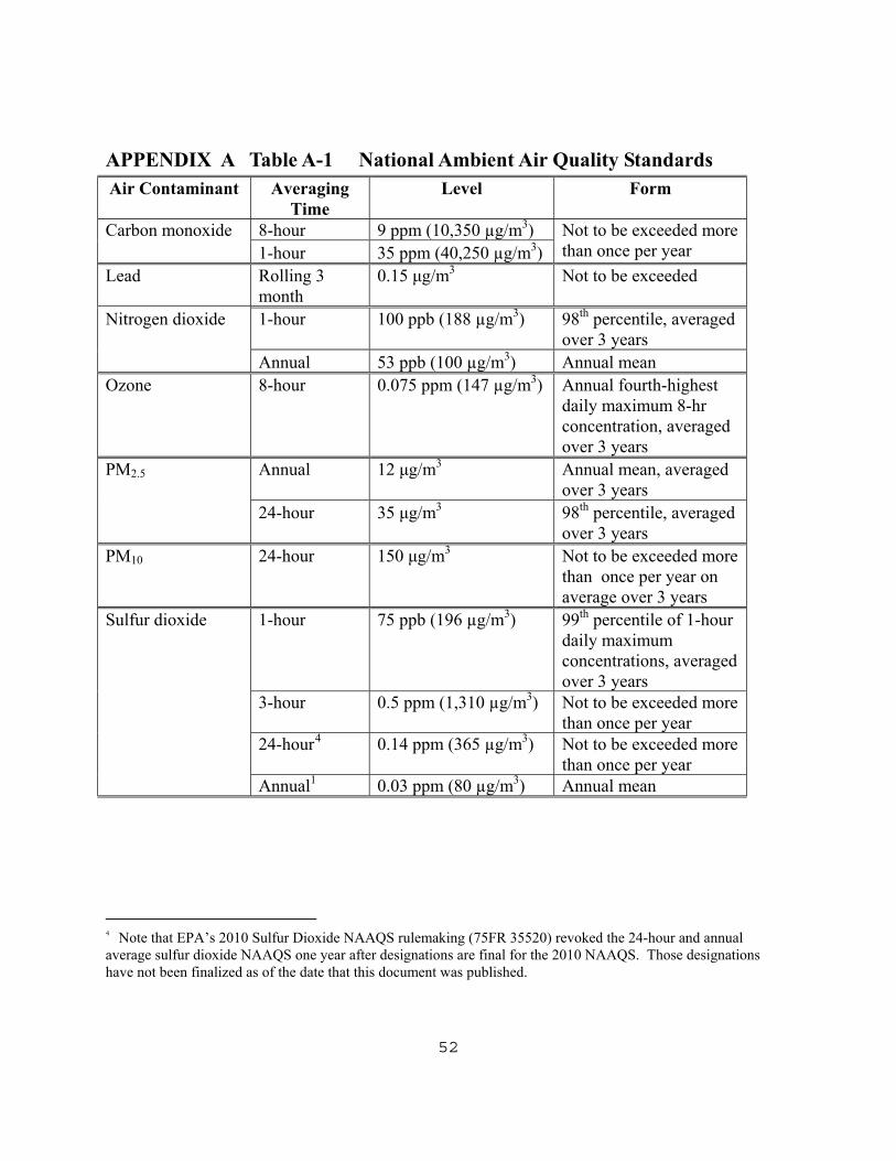
52

APPENDIX A Table A-1 National Ambient Air Quality Standards Air Contaminant Averaging

Time Level Form

8-hour 9 ppm (10,350 µg/m3) Carbon monoxide 1-hour 35 ppm (40,250 µg/m3)

Not to be exceeded more than once per year

Lead Rolling 3 month

0.15 μg/m3 Not to be exceeded

1-hour 100 ppb (188 µg/m3) 98th percentile, averaged over 3 years

Nitrogen dioxide

Annual 53 ppb (100 µg/m3) Annual mean Ozone 8-hour 0.075 ppm (147 µg/m3) Annual fourth-highest

daily maximum 8-hr concentration, averaged over 3 years

Annual 12 μg/m3 Annual mean, averaged over 3 years

PM2.5

24-hour 35 μg/m3 98th percentile, averaged over 3 years

PM10 24-hour 150 μg/m3 Not to be exceeded more than once per year on average over 3 years

1-hour 75 ppb (196 µg/m3) 99th percentile of 1-hour daily maximum concentrations, averaged over 3 years

3-hour 0.5 ppm (1,310 µg/m3) Not to be exceeded more than once per year

24-hour4 0.14 ppm (365 µg/m3) Not to be exceeded more than once per year

Sulfur dioxide

Annual1 0.03 ppm (80 µg/m3) Annual mean

4 Note that EPA’s 2010 Sulfur Dioxide NAAQS rulemaking (75FR 35520) revoked the 24-hour and annual average sulfur dioxide NAAQS one year after designations are final for the 2010 NAAQS. Those designations have not been finalized as of the date that this document was published.

53

APPENDIX B AIR DISPERSION MODELING PROTOCOL CHECKLIST

Air Dispersion Modeling Protocol Checklist (Please refer to Section 5.1 of this guidance) 1) Project description Yes No Project parameters Yes No Regulatory requirements Yes No Air quality analysis Yes No Modeling results Yes No Special Modeling Considerations Yes No 2) Air Dispersion Model

AERMOD AERSCREEN 3) Land Use Designation Urban Rural 4) Years and Location of Meteorological Data Used.

AERSCREEN Default Data Yes No 5 Years TF Green/Chatham Data from OAR Yes No Facility On-Site Meteorological Data Yes No

5) Anemometer height: (TF Green anemometer is 10 m) 6) Background Air Quality Data

Must contact the OAR to obtain the latest background concentrations for use in Rhode Island.

7) Receptor Spacing

Discrete receptors should be placed along property boundaries at 10-meters intervals. Beyond the property line, receptors should be placed at 25-meter intervals out to 1000 meters, 100-meter intervals out to 2,000 meters, and 200-meter intervals out to 2,000 meters

8) Terrain Elevation Data to be Used

USGS DEM/NED (datum year: ______) Survey Data Other: __________ 54

North American Datum: 1927 1983 9) Stack Orientation

Are all stacks vertical and unobstructed? Yes No If no, refer to Section 7.3 of this guidance

10) Interacting Sources for Criteria Pollutant Analyses

Will interacting sources be modeled? Yes No If yes, please provide an approximate Significant Impact Area: Radius of (m)____________around the subject source

11) Information included in electronic media

An electronic copy of input files and output files associated with the highest impacted met year must be included with your modeling submission.

55