rhessys: regional hydro-ecologic simulation … current version of rhessys continues to follow the...

Copyright � 2004, Paper 0-019; 14,552 words, 5 Figures, 0 Animations, 2 Tables.

http://EarthInteractions.org

RHESSys: Regional Hydro-EcologicSimulation System—An Object-Oriented Approach to SpatiallyDistributed Modeling of Carbon,Water, and Nutrient Cycling

C.L. Tague*Department of Geography, San Diego State University, San Diego, California

L.E. BandDepartment of Geography, University of North Carolina at Chapel Hill, Chapel Hill,

North Carolina

Received 29 October 2003; accepted 3 February 2004

ABSTRACT: Process-based models that can represent multiple andinteracting processes provide a framework for combining field-based measure-ments with evolving science-based models of specific hydroecologicalprocesses. Use of these models, however, requires that the representation ofprocesses and key assumptions involved be understood by the user community.This paper provides a full description of process implementation in the mostrecent version of the Regional Hydro-Ecological Simulation System(RHESSys), a model that has been applied in a wide variety of research

* Corresponding author address: C.L. Tague, Department of Geography, San Diego State

University, 5500 Campanile Drive, San Diego, CA 92182-4493.

E-mail address: [email protected]

Earth Interactions � Volume 8 (2004) � Paper No. 19 �

settings. An overview of the underlying (Geographic Information System) GIS-based model framework is given followed by a description of the mathematicalmodels used to represent various biogeochemical cycling and hydrologicprocesses including vertical and lateral hydrologic fluxes, microclimatevariability, canopy radiation transfer, vegetation and soil microbial carbonand nitrogen cycling. An example application of RHESSys for a small forestedwatershed as part of the Baltimore Long-Term Ecological Research site isincluded to illustrate use of the model in exploring spatial-temporal dynamicsand the coupling between hydrology and biogeochemical cycling.

KEYWORDS: Hydrology, Modeling, Ecosystems

1. Introduction

The Regional Hydro-Ecological Simulation System (RHESSys) is a hydro-ecological model designed to simulate integrated water, carbon, and nutrientcycling and transport over spatially variable terrain at small (first-order streams) tomedium (fourth- and fifth-order streams) scales. The model is structured as aspatially nested hierarchical representation of the landscape with a range ofhydrological, microclimate, and ecosystem processes associated with specificlandscape objects at different levels of the hierarchy. This approach is designed tofacilitate environmental analysis that requires an understanding of within-watershed processes as well as aggregate fluxes of water, carbon, and nitrogen.

As a hydrologic model, RHESSys is intermediate in terms of complexity. Unlikelumped parameter hydrologic models such as the Identification of unit Hydro-graphs and Component flows from Rainfall, Evaporation, and Streamflow data(IHACRES; Evans and Jakeman 1998) or empirical curve number approaches,RHESSys explicitly models connectivity and lateral hydrologic fluxes betweenlandscape units within a watershed. The representation of the vertical soil profile,however, is based on a fairly simple two-layer model with a single unsaturated andsaturated zone. Additional hydrologic stores include a litter layer, surface detentionstore, multiple canopy interception layers, and a snowpack. Process-basedhydrologic models such as MIKE-SHE (Refsgaard and Storm 1995) are at themore complex end of the continuum and provide a 1D Richard’s equation solutionto drainage through multiple soil layers down to the saturated zone. In addition tohydrology, RHESSys is able to model feedbacks between hydrology andecosystem carbon and nutrient cycling, including the growth of vegetation. Otherprocess-based eco-hydrologic models such as Macaque (Watson et al. 1999) andTopog (Vertessy et al. 1993) also provide this capability. In each of these models,representation of specific processes may differ but these models are relativelysimilar in terms of overall complexity.

The version of RHESSys described in this paper has evolved from theintegration of stand-level ecosystem models with methods to compute thedistribution and flux of soil water at the landscape level. These earlier versionsof RHESSys were designed to explicitly couple the Forest Biogeochemical Cycles(FOREST-BGC) canopy model (Running and Coughlan 1988) with landscape-level patterns of critical meteorological forcing (Running et al. 1987) and later withhydrologic processes using the TOPMODEL (Beven and Kirkby 1979) hydrologicmodel. The first approach to distribute ecosystem processes at the landscape level


involved gridding the ‘‘topclimatic’’ logic of Mountain Climate Simulator (MTN-CLIM) with FOREST-BGC for a 1200 km2 watershed in western Montana(Running et al. 1987). Later versions of RHESSys followed a generalization ofFOREST-BGC to multiple biomes as Biome biogeochemical cycles Model(BIOME-BGC) (Running and Hunt 1993). Hydrologic modeling studies usingRHESSys have included analysis of model sensitivity to landscape representation(Band 1993; Band et al. 1993) and using the model to explore the sensitivity ofhydrologic response to climate change (Baron et al. 1998).

This current version of RHESSys continues to follow the basic BIOME-BGCframework. As discussed in this paper, however, many submodels used for specificprocesses have been altered and/or extended, largely to improve the soilbiogeochemical process representation and expand canopy representation to considerboth understory and overstory layers. Representation of soil organic matter decom-position in both RHESSys and BIOME-BGC is based largely on the CENTURYmodel. RHESSys also uses the CENTURYNGAS (Parton et al. 1996) approach tomodel (nitrogen) N-cycling processes such as nitrification and denitrification.

The current version of RHESSys has extended these hydrologic studies throughthe incorporation of an explicit hydrologic routing model in place of TOPMODEL.This current version has been used to explore the combined impact of roads andforest harvesting for several catchments in the Pacific Northwest (Tague and Band2001; Krezek 2001), as well as in the Canadian boreal plain (Creed et al. 2000).

Coupled hydrologic-ecosystem and biogeochemical cycling studies usingRHESSys include Mackay and Band (Mackay and Band 1997) who applied anearlier version of RHESSys to estimate carbon cycling in a small forestedwatershed. Mitchell and Csillag (Mitchell and Csillag 2000) are using the currentversion of RHESSys to explore spatially varying soil moisture controls ongrassland productivity. Creed and Band (Creed and Band 1998) illustrate the use ofsimilarity indices, derived using an earlier version of RHESSys, to compute anitrate-flushing index based on saturation and a source index based on nitrateavailability and dynamics in the saturation zone for a set of forested catchments inOntario, Canada. By using these similarity indices, Creed and Band (Creed andBand 1998) were able to explain a significant amount of the variation in nitrateexport between catchments and over time within the region. These indices,however, did not explicitly model N cycling and transport dynamics. Explicitmodeling of N cycling and transport dynamics is included in the current version ofRHESSys and has been tested for a small forested watershed as part of theBaltimore Ecosystem Study (BES; Band et al. 2001). The current version is alsobeing used to explore spatial variation in N cycling in the Rocky Mountains(Laundrum et al. 2002), N saturation in the Smokey Mountains (Webster et al.2001), and to examine the alteration of N sources and sinks along hydrologicflowpaths along a gradient of urbanization as part of the BES (Tague et al. 2000).

2. Implementation and model structure

One of the unique features of RHESSys is its hierarchical landscape representation.This approach allows different processes to be modeled at different scales andallows basic modeling units to be of arbitrary shape rather than strictly grid based.


RHESSys is also structured using an object-based design approach to facilitatealgorithmic substitution. Additional details on model hierarchical structure andcoding implementation can be found in Band et al. (Band et al. 2000).

RHESSys partitions the landscape such that each level of the spatial hierarchyfully covers the spatial extent of the landscape. Spatial levels define a containmenthierarchy with progressively finer units. Each spatial level is associated withdifferent processes modeled by RHESSys and with a particular scale. At the finestscale, patches are typically defined on the order of meters squared, while basins(km2) define the largest scale.

Within RHESSys, a given spatial level is defined as a particular object type witha set of state (storage) and flux variables, process representations (equation sets),and an associated set of model parameters. For example, the estimation ofatmospheric flux variables such as radiation occurs at the zone level. Thus, inderiving the set of spatial objects for a given simulation, zones are chosen torepresent areas of similar climate or atmospheric-forcing conditions. The advantageof this hierarchical approach is that it allows different processes, that is, climateversus canopy processes, to be modeled at different spatial and temporal scales. Italso allows modeling to occur on ecologically meaningful units as opposed toarbitrarily defined grid cells.

The definition of modeling units is done by the user prior to running thesimulation. Although the user is given considerable flexibility in choosing apartitioning strategy for the different levels, partitioning should be tailored to takeadvantage of the patterns of relevant variability within the landscape and, in the caseof patches, to maintain a coherent and solvable flow network. This permits efficientparameterization and reduces the error associated with landscape partitioning. Bandet al. (Band et al. 1991), Lammers et al. (Lammers et al. 1997), and Tague et al.(Tague et al. 2000) provide further justification for and discussion of partitioningstrategies, although this is an area requiring additional development.

2.1. Basins

Basins are defined as hydrologically closed drainage areas and encompass a singlestream network. Basins typically serve as aggregating units to determine net fluxesof carbon, water, and nitrogen over the entire study area.

At present, RHESSys accounts for routing (storage and flux) of water withinhillslopes to the stream. Once water reaches the stream, however, it is assumed toexit the basin within a single (daily) time step. For larger basins or shorter timesteps, in-stream channel processes can be important. Future versions of RHESSyswill likely use basins to organize the combination of hillslopes and stream reachesas separate object types and include a channel-routing model for stream reacheswithin the basin stream network.

2.2. Hillslopes

Hillslopes define areas that drain into one side of a single stream reach. Explicitrouting between patches is organized at the hillslope level to produce streamflow.Hillslopes will usually be derived based upon drainage patterns using (GeographicInformation System) GIS-based terrain-partitioning algorithms such as r.watershed


in GRASS (Geographic Resources Analysis Support System) GIS environmentand as described in Lammers and Band (Lammers and Band 1990). Like basins,hillslopes can also be used to aggregate sublevel processes. The spatialredistribution of patch soil moisture is organized at the hillslope level and, forsimulations that use TOPMODEL for lateral flow distribution, a hillslope-levelbase flow is defined.

2.3. Zones

Zones denote areas of similar climate. Zone objects contain meteorologicalvariables and use topclimate extrapolation methods necessary to characterize spatialvariation in these variables. Each zone is linked to a particular set of climate inputfiles. Thus, a given landscape may use data from multiple meteorological stations oratmospheric model grid cells if this information is available. Data from a particularstation are modified based on zone elevation, slope, and aspect relative to the inputclimate station. Zone processing also estimates additional climate variables thatmay not be available from base climate station information such as vapor pressuredeficit. Numerous strategies exist to partition areas of similar climate. Elevationbands in a mountainous area, for example, are likely to denote areas of similarclimate and exposure as discussed in Lammers et al. (Lammers et al. 1997). Thedistribution of climate stations can also be used to define zone partitioning, whereeach zone defines the area associated with a particular climate station.

2.4. Patches

Patches represent the smallest-resolution spatial unit and define areas of similar soilmoisture and land-cover characteristics. Vertical soil moisture processing and soilbiogeochemistry are modeled at the patch level. Patch variables include fluxes suchas infiltration, saturation zone recharge, and soil nutrient cycling. Patches are oftenderived using an overlay of several different maps, such as a wetness index,vegetation cover, and stream and road network layers. Patch definition, however,must also be designed to maintain the underlying topographic controls on drainagepatterns in the watershed. Patches can be defined that contain a stream channel andparameterized to regulate land-channel drainage flux. In landscapes modified byhumans, patches may also be defined to contain a stream channel, road segments,or storm sewers that provide specific drainage conditions. Human sources of waterand nutrients including irrigation, fertilization, and septic system input are alsodefined at this level.

2.5. Canopy strata

Canopy strata are a separate object type but they define vertical, abovegroundlayers rather than horizontal spatial layers. The spatial resolution of the canopystratum is defined by the patch partitioning. Processes such as photosynthesis andtranspiration are modeled at the canopy stratum level. Each stratum corresponds toa different layer such as overstory or understory in the canopy structure. The userdefines the number of vertical layers. A height state variable is associated with eachlayer and defines its processing relative to the other layers. Incoming radiation,


precipitation throughfall, and wind are extinguished through the multiple layersaccording to the height and vegetation characteristics of each layer. RHESSys alsopermits multiple strata at the same height. This allows mixed vegetation typeswithin the same spatial area to be represented. Finally, a litter layer is defined at thepatch level and receives input from the overlying canopy layers. This litter layeracts as the interface between each patch and its associated canopy strata layers. Fornonvegetated patches, a dummy litter layer (with no attenuation or processing ofhydrologic, energy and carbon/nutrient fluxes) is used.

2.6. Interface

Parameterization and management of RHESSys is complex due to the multiplelevels of spatial partitioning and the associated parameter sets. Most of theseparameters are derived from topographic, land-cover, and soil map layers.Associated with RHESSys are a number of interface programs, which organizeinput data into the format required by the simulation model. These include standardGIS-based terrain-partitioning programs and RHESSys-specific programs thatderive landscape representation from GIS images and establish connectivitybetween spatial units. These various programs can be run in stand-alone mode or aspart of an integrated RHESSys interface, RAINMENT. Additional details about theRHESSys interface can be found in Band et al. (Band et al. 2000).

Key inputs into RHESSys include (see Figure 1) the following.

1. A description (worldfile) of the landscape representation and initial-statevariables associated with each component of the spatial hierarchy (i.e.,basins, hillslopes, zones, etc.) Because of the length and spatial complexityincorporated in this description, GRASS and ARCVIEW GIS-basedprograms (GRASS2WORLD, ARCVIEW2WORLD) were developed togenerate this file.

2. The flow table describes connectivity between patches within a hillslopewhen the explicit routing approach is used to model distributed hydrology.The flow table is also generated automatically prior to running the mainRHESSys simulation using a software program (CREATE-FLOWPATHS).

3. The temporal event control (TEC) file describes the timing and nature oftemporal events that will occur during the course of the simulation, that is,disturbances such as forest harvesting, fire, or road construction. Temporalevents refer to events that initiate a change in landscape-state variables orparameterization or new processes in the simulation sequence. A spinupperiod is typically run prior to output to remove transient behavior due toinitialization.The TECfile is also used to control data assimilation for output.

4. Time series inputs include a range of climate variables as discussed insection 3, along with descriptions of the station at which this informationwas collected. Each zone in the spatial hierarchy is associated with aparticular climate station. Note that base station coverage can be defined atany level of the hierarchy and need not be spatially contained by hillslopes,zones, or patches. Input stations can also be assigned at the patch level toorganize fertilizer and irrigation inputs.

5. Parameter files are associated with each level of the spatial hierarchy. A


library of commonly used parameter files assigned to specific soil andvegetation types is available. The current library of parameter files includestandard parameters for conifer, deciduous, grass, chaparral, tundra, as wellas a number of more refined files for specific species groups such maple,pine, spruce, oak, aspen, or douglas fir. The current library of parameterfiles include all major soil textures, such as clay, sandy loam, etc.

2.7. Implementation and future development

This current version of RHESSys is implemented in the C programming languageusing an object-based approach to facilitate the substitution of different processalgorithms. All of the processes as well as input/output routines are contained inseparate procedures with appropriate names. This allows for relatively easymodification of specific process algorithms. Data structures are similarly definedand named to maintain clarity about the level of the spatial hierarchy associatedwith a specific algorithm.

The object-based approach and hierarchical landscape representation are alsodesigned to facilitate future RHESSys development. Structures exist to allow forthe development of subdaily time step models for certain processes such asinfiltration. Object-based landscape representation also facilitates the implementa-tion of different land covers such as those found in urban areas. Hillslope-levelorganization of drainage and particularly the implementation of roads asmechanisms by which flow can be redirected serve as a foundation forimplementation of other man-made controls on flowpaths such as sewers.

3. Atmospheric and environmental forcing

Atmospheric variables or external forcing variables drive RHESSys hydrology andbiogeochemical cycling. These include climate variables such as daily temperature

Figure 1. RHESSys model structure: Inputs, output, and preprocessing.


and precipitation as well as material inputs such as atmospheric nitrogendeposition. Climate input and processing in RHESSys is done at the zone level.Each zone is assigned a particular base station that manages external time seriesinputs to the model. Multiple zone objects can be assigned to the same base station;however, each zone must have a unique base station associated with it. Theappendix lists current atmospheric variables that are used internally in the model.For most of these variables, the user has the option of providing a daily time seriesas input (associated with its base station) or allowing RHESSys to estimate thedaily value from user parameters. Daily temperature and precipitation, however,must be input by the user. Input time series may be derived from field observationor from coupling with external models. Internal estimation of most meteorologicalvariables, including incoming radiation, is based on algorithms from the MTN-CLIM model (Running et al. 1987).

Currently, nitrogen and precipitation are the only material inputs into the model.Atmospheric nitrogen deposition as nitrate and as ammonium are input as separatetime series in RHESSys. Wet and dry deposition, however, are not distinguished inthe current model. If a time series of nitrogen deposition is not provided, a constantdaily value for nitrate based on a zone parameter will be used. In this case,deposition as ammonium is assumed to be zero.

3.1. Temperature

Daily minimum and maximum temperature time series must be included in thebase station assigned to each zone object. Note that these time series may bederived from field observations or from an external mesoscale atmospheric modelsuch as the Regional Atmospheric Modeling System (RAMS; Walko et al. 2000)or external climate interpolation schemes such as the Parameter-ElevationRegressions on Independent Slopes Model (PRISM; Daly et al. 1994) or Daymet(Thornton et al. 1997). For each zone, the base station temperatures are scaled by alapse rate with elevation (included as a zone parameter).

Dewpoint temperature, if it is included with base station data, is similarlyadjusted by a dewpoint lapse rate. If it is not input as a time series, it is assumed tobe the minimum temperature value, after the elevation adjustment. Rooting zonesoil temperature is computed as a running average of average air temperaturesimilar to Zheng et al. (Zheng et al. 1993):

TsoilðtÞ ¼ 0:9 Tsoilðt�1Þ� �

þ 0:1ðTavgÞ; ð1Þwhere Tsoil is rooting zone soil temperature and Tavg is average daily temperature.The buffering effect of snow cover is not taken into account.

3.2. Precipitation

A daily precipitation time series must also be included in each base station and can beadjusted using an isohyetal multiplier assigned to each zone. Orographic patterns inprecipitation can be modeled using this isohyetal multiplier. Rainfall durationdefaults to the entire day, unless a rainfall duration time series is included as a basestation input. The user also has the option of providing hourly, rather than daily,rainfall input and running the hydrologic portion of the model in an hourly mode.


The user may input a snowfall time series directly. If a snowfall time series is notincluded, precipitation is partitioned into rain and snow by assuming a lineartransition from snow to rain across a temperature range defined by Tminrain andTmaxsnow , which are zone parameters indicating the minimum temperature at whichrain can occur and the maximum temperature at which snow can occur,respectively.

3.3. Vapor pressure deficit

Saturation vapor pressure and relative humidity can be input directly. If theseobservations are not available from the base station climate file, saturation vaporpressure and vapor pressure deficit are estimated from standard air temperature–vapor pressure relationships (Jones 1992).

3.4. Incoming radiation

Canopy radiation interception (see section 5.2.) depends upon top of canopyinputs of both diffuse (Kdiffuse0) and direct (Kdirect0) solar radiation as well aslongwave radiation. These radiation streams can be input by the user as part ofthe climate base station or can be estimated internally in the model. WithinRHESSys, a solar geometric-based estimate of atmospheric radiation is computedbased on site latitude, zone slope, aspect, and east–west horizon values. Incomingradiation is then adjusted to account for atmospheric transmissivity, estimatedbased on daily temperature variation and precipitation. These equations are notdescribed here since they directly follow the MTN-CLIM approach (Running etal. 1987).

3.5. Atmospheric CO2

In the current version of RHESSys, atmospheric CO2 concentration is heldconstant at 370 ppm. (Note: CO2 concentration is used in estimates of stomatalconductance.) It is included as a state variable, however, such that it can be readilymodified in future versions.

4. Soil hydrologic processes and transport mechanisms

Vertical and lateral soil moisture and associated nutrient fluxes are modeled foreach patch object. Patch topology (i.e., connectivity between patches) is organizedby basin objects.

To model vertical soil moisture processes, a simple three-layer model is used,which includes a surface detention store, an unsaturated store, and a saturated store.Snowpack and litter stores are also included.

Water can also be stored in the vegetation and litter layers above each patch asinterception storage (see section 5.5.). The soil column consists of two variabledepth layers: an unsaturated zone and a saturated zone. The boundary between thesaturated and unsaturated zone is defined by the saturation deficit (s as a waterequivalent deficit and z as an actual depth to saturation). Vertical fluxes betweeneach soil compartment are modeled to preserve mass balances such that, for eachtime step


�s ¼ �qdrain þ qcap þ ETsat ð2Þ�sunsat ¼ qinfil � qdrain þ qcap � ETunsat ð3Þ�detS ¼ TFþ qmelt � qinfil � E; ð4Þ

where qdrain, qcap, and qinfil are drainage from the unsaturated zone, capilliary rise,and infiltration, respectively; ETsat and ETunsat are evapotranspiration from thesaturated and unsaturated zone, respectively; sunsat is the soil moisture content of theunsatured zone and detS is the surface detention storage; TF is the net throughfallfrom canopy layers; E is the surface storage evaporation; and qmelt is snowmelt. Allstores are maintained as meters of water and fluxes as meters per day.

4.1. Detention storage and infiltration

At each time step, net throughfall from canopy layers and snowmelt are added tocurrent surface detention storage and allowed to infiltrate into the soil followingPhillip’s infiltration equation (Phillip 1957):

qinfil ¼ Itp þ Spffiffiffiffiffiffiffiffiffiffiffiffiffitd � tp

pþ Ksatsðtd � tpÞ for td > tp;

qinfil ¼ Itd for td , tp; ð5Þwhere qinfil is infiltration; I and td are input intensity and duration; and Ksats issaturated hydraulic conductivity at the wetting front, defined by the saturationdepth z. [Equation (8) is used to compute Ksats at depth z.] Estimation of sorptivitySp is based on Manley (Manley 1977):

Sp ¼ffiffiffi2

pKsats0:76uae; ð6Þ

where uae is air entry pressure, which is set as a soil specific input parameter.Time to ponding is denoted as tp, which is computed using the Green and Ampt

approximations (Green and Ampt 1911) as follows:

tp ¼ Ksats0:76uae

ð/� h0ÞIðI � KsatsÞ

; ð7Þ

where / is porosity and h0 is initial soil moisture content.If a daily time step is used, it is assumed that all inputs (precipitation and

snowmelt) are distributed evenly throughout the day. In regions characterized byhigh-intensity, short-duration rainfall, this approach will overestimate infiltrationrates. In these cases, the user may choose to input a rainfall duration time series,which will override the assumption of a daily duration.

Ponded water that is not infiltrated within the daily time step becomes detentionstorage. Detention storage beyond a surface detention storage capacity parameterwill become overland flow.

4.2. Hydraulic conductivity and porosity profiles

The vertical hydraulic conductivity profile controls both vertical and lateral soilmoisture fluxes in RHESSys. In the current implementation an exponential profile isthe default; although alternative profiles may be substituted for specific field siteswhere the soil conductivity profile does not fit this exponential mode (e.g.,


Ambroise et al. 1996). Thus, saturated hydraulic conductivity, Ksat(z) is computed as

KsatðzÞ ¼ Ksat0 expð� z

mÞ; ð8Þwhere Ksat0 is hydraulic conductivity at the surface and m describes the decay rate ofconductivity with depth. Both are set as soil-type-specific input parameters.Hydraulic conductivity profiles are difficult to measure and may vary widely for agiven soil texture/type. Further, field evidence suggests that at scales greater thancentimeters, conductivity controls on hydrologic fluxes must consider both theproperties of the soil matrix and macropore/preferential flowpath distributions(McDonnell 1990). To account for both uncertainty in conductivity profiles andpreferential flow, both m and Ksat0 are typically calibrated against observedstreamflow values in RHESSys (see section 7).

Porosity is also permitted to vary with depth such that

/ðzÞ ¼ /0 exp�zp; ð9Þ

where /0 and p are soil specific parameters defining surface porosity and the decayof porosity with depth, respectively. Setting a large value of p (e.g., p . 1000.0)allows a constant porosity to be assumed. Saturated soil moisture storage for a givenprofile section must be calculated by integrating porosity over the associated depth.

4.3. Vertical unsaturated zone drainage

As noted above, RHESSys maintains both an unsaturated and saturated zone.Drainage from the unsaturated zone to the saturated zone, qdrain, is limited by fieldcapacity hfc of the unsaturated zone (computed by integrading a pressure gradientof �1 over the unsaturated profile), and by the vertical unsaturated hydraulicconductivity at the boundary [KunsatðzÞ] between the unsaturated and saturated zonesuch that

qdrain ¼ min½KunsatðzsÞdT; hunsat � hfc�; ð10Þwhere dT is the time step.

Here KunsatðzÞ can be estimated using either vanGenuchten and Nielsen(vanGenuchten and Nielsen 1984) or Clapp and Hornberger (Clapp andHornberger 1978) models of soil characteristics.

In the Clapp and Hornberger (Clapp and Hornberger 1978) approach:

KunsatðzÞ ¼ KsatðzÞSð2bþ3Þ; ð11Þwhere b is the pore size index, a soil-specific parameter; Ksat0ðzÞ is calculated usingEquation (8), and S is relative saturation.

If the vanGenuchten approach is used:

KunsatðzÞ ¼ Ksat0ðzÞS0:5½1� ð1� S1cÞc�2; ð12Þ

where c is a soil-specific parameter.To compute a depth of unsaturated zone soil moisture at field capacity [hfc in

Equation (10)], the relative saturation at field capacity is integrated over theporosity profile from the surface to the water table depth (zs).

Relative saturation at field capacity Sfc is derived again based on either the Clapp


and Hornberger (Clapp and Hornberger 1978) or vanGenuchten and Nielsen(vanGenuchten and Nielsen 1984) assumptions such that, respectively,

SfcðzÞ ¼uae

ðzs � zÞ

� �b; ð13Þ

SfcðzÞ ¼ 1� ðzs � zÞucae

�b" #

: ð14Þ

Note that b and c are the soil-specific parameters used in Equations (11)–(12)above, uae is the air entry pressure, again assigned based on soil type.

4.4. Soil evaporation

Soil evaporation is limited both by energy and atmospheric drivers and by amaximum exfiltration rate as a function of soil properties at a given soil moisture.

Soil moisture limits on soil evaporation are accounted for using a potentialexfiltration rate, potqexfil , based on a modification of Eagleson (Eagleson 1978) byWigmosta et al. (Wigmosta et al. 1994) such that

potqexfil ¼ S12b

ffiffiffiffiffiffiffiffiffiffiffiffiffiffiffiffiffiffiffiffiffiffiffiffiffiffiffiffiffiffiffiffiffiffiffiffi8 �/�Ksatuae

3ð1þ 3bÞð1þ 4bÞ

s" #; ð15Þ

where b is the pore size index. Porosity ( �/) and saturated hydraulic conductivity(�Ksat) are averaged over depth to saturation (zs) using Equations (9) and (8),respectively, and S is the relative soil moisture content computed as (unsat/s) withan added restriction of a maximum active soil depth over which the exfiltrationprocess applies. Thus, if the saturation deficit is greater than an active soil depth,the relative soil moisture S is computed as unsat/sactive.soil.depth. Active soil depth isincluded as a soil-specific parameter.

Energy and atmospheric drivers of soil evaporation are accounted for using thePenman–Monteith equation (see section 5.6.). Surface conductance for soil isbased on empirical relationships between rooting zone soil water content h anddiffusive resistance Csurf, as observed by Kelliher et al. (Kelliher et al. 1986) in adouglas fir forest:

Csurf ¼ 0:001 429 for h > 0:185;

Csurf ¼1

�83 000hþ 16 100for 0, h, ¼ 0:185; and

Csurf ¼ 9 999 999 for h ¼ 0: ð16ÞClearly, generalization of this empirical model to other sites may requireadjustment. In arid or sparsely vegetated environments where soil evaporationcan be a significant component of the water balance, substitution of local empiricalrelationships may be necessary.

Final soil evaporation is a minimum of rates based on the Penman potentialevaporation and soil exfiltration rates.


4.5. Capillary rise

Potential capillary rise is based upon the approach used by Eagleson (1978) such that

qcap ¼ Ksatzs1þ 1:5

ð1þ 3bÞuae

ðzs � uaeÞ

� �ð2þ3bÞ; ð17Þ

whereKsatzs is the hydraulic conductivity at thewater table depth (zs) [computed usingEquation (8)]; b and uae are pore size index and air entry pressure, respectively, andare set based on soil type.

Capillary rise is limited to filling unsaturated zone to field capacity. To correctfor subdaily plant responses, one-half of the potential capillary rise, computedusing Equation (17) is allocated to the unsaturated zone at the start of the day. Theremaining potential is available later in the day to satisfy plant transpirationdemands (see section 5.6.).

4.6. Snow accumulation and melt

Snow accumlation is based on incoming precipitation and is assumed to fall evenlyover each climate zone. Modeling case studies using previous versions ofRHESSys, however, have shown that in snow-dominated environments, theredistribution of snow by wind, can have a significant impact on hydrology(Hartman et al. 1999). In the current model, we do not account for this effect;however, an adaptation of a more sophisticated snow accumulation and meltapproach will likely be included in future versions.

Snowmelt, qmelt, is computed using a quasi–energy budget approach that takesinto account radiation (Mrad), a combination of melt due to sensible and latent heatflux (MT), and advective (MV) (from rain on snow) controls on snowmelt such that,at the daily time step

qmelt ¼ Mrad þMT þMV : ð18ÞMelt from temperature and advection occur only when the snowpack is ripe.Snowpack temperature is approximated using an air temperature accumulation of asnowpack energy deficit (SED):

SEDt ¼ max SEDðt�1Þ þ Tair; SEDmax

� �; ð19Þ

where SED(t� 1) is the previous day’s energy deficit, Tair is mean daily temperature,and SEDmax is a maximum energy deficit that is set as a climate-region-specificinput parameter. Melt due to radiation can occur as sublimation when the energydeficit SED is less than 0.

Radiation melt is computed as

Mrad ¼ðKdirect þ Kdiffuse þ LÞ

kfqwaterfor ðSED >¼ 0Þ;

Mrad ¼ðKdirect þ Kdiffuse þ LÞ

ðkf þ kvÞqwaterfor ðSED, 0Þ; ð20Þ

where kv and kf are the latent heat of vaporization and and fusion, respectively;qwater is the density of water; Kdirect and Kdiffuse are direct and diffuse shortwave


radiation absorbed by the snowpack; and L is longwave radiation. Direct anddiffuse shortwave radiation absorption by the snowpack is computed based on aBeer’s law extinction model of available radiative fluxes (Kdirect0 and Kdiffuse0) andaccounts for albedo-driven reflectance at the level of the snowpack. This approachis used to maintain consistency with radiation attenuation through vertical canopylayers as described in section 5.2. Thus,

Kdirect ¼ ð1� aÞKdirect0ð1� exp�ksnowÞ: ð21ÞThe extinction coefficient ksnow is input as a climate-specific default. Setting k to anarbitrary large value will ensure that all nonreflected radiation will be absorbed bythe snowpack. Snowpack reflectance or albedo a is estimated based upon asnowpack surface age following Laramie and Schaake (Laramie and Schaake1972):

a ¼ 0:85 0:82Age0:46

� �for ðSED >¼ 0Þ;

a ¼ 0:85 0:94Age0:58

� �for ðSED, 0Þ; ð22Þ

where ‘‘Age’’ is the number of days since last snowfall. A similar approach is usedto account for diffuse radiation fluxes.

Longwave radiation into the snowpack is estimated from air temperaturefollowing Croley (Croley 1989):

L ¼ 41:868 essatmr ðTair þ 272Þ4� 663h i

for ðSED >¼ 0Þ and ðTair >¼ 0Þ;

L ¼ 41:868 ðessatm � 1Þr ðTair þ 272Þ4� 663h i

for ðSED, 0Þ and ðTair , 0Þ; ð23Þ

where r is the Stefan–Boltzmann constant. Atmospheric emissivity essatm isadjusted for overstory canopy (Dingman 1994) and cloud fraction (CF; Croley1989):

essatm ¼ ð1� FÞ 0:53þ 0:065ea

0:5

100ð1þ 4:0CFÞ þ F

� �; ð24Þ

where F is the fractional canopy cover over the snowpack and ea is the atmosphericvapor pressure. If cloud fraction data are not available, the cloud fraction isassumed to be 1.0 for days with precipitation and 0.0 for dry days.

Melt due to latent and sensible heat flux is based on an empirical relationshipwith air temperature (Coughlan and Running 1997) that is adjusted for the effectsof variation in wind speed due to the fractional forest cover F over a snowpack(Dunne and Leopold 1979)

MT ¼ bMTTairð1� 0:8FÞ; ð25Þwhere bMT is an empirical temperature melt coefficient that is input as a climate-region-specific parameter.

Advection melt contributions due to warming by incoming precipitation arecomputed as

MV ¼ qwaterTairTFcpwaterð Þ=kf ; ð26Þ


where TF is net throughfall entering the snowpack, and cpwater and qwater are theheat capacity and density of water, respectively.

4.7. Lateral redistribution

Soil moisture redistribution through saturated throughflow and associated runoffproduction can be modeled using either a quasi-spatially distributed model,TOPMODEL (Beven and Kirkby 1979) or via an explicit routing model, which is amodification of the Distributed Hydrology Soil Vegetation Model (DHSVM;Wigmosta et al. 1994).

TOPMODEL is applied at the hillslope level. DHSVM is applied at the basinlevel, since it can include some limited streamflow routing. Both approaches areexecuted at the end of the day, following vertical soil moisture updates.

4.7.1. TOPMODEL

TOPMODEL is a statistically based approach that redistributes saturation zonewater based on an index of hydrologic similarity. As a statistically based approach,TOPMODEL represents a simplified approach that has been applied and tested innumerous catchments. TOPMODEL relationships are based on the assumption thatsaturated hydraulic conductivity varies exponentially with depth, that water tablegradients can be approximated by local topographic slope, and that steady-stateflux is achieved within the modeling time step. TOPMODEL distributes a meansoil moisture deficit, �s based on a local wetness index wi:

wi ¼ lnarTe

To tanb; ð27Þ

where Te and To are the mean and local hillslope saturated transmissivity,respectively, tanb is the local slope, and ar is the upslope contributing area.

Local saturation deficit si for each patch, is computed as

si ¼ �sþ msð�w� wiÞ; ð28Þwhere �w is mean hillslope wetness index value, �s is the mean hillslope saturationdeficit, and ms describes a decay rate of hydraulic conductivity with saturationdeficit. Transmissivity TR is computed as

Tr ¼Z zsat

�‘

Ksat0 exp� smsdz; ð29Þ

where Ksat0 is saturated hydraulic conductivity at surface.Alternatively, a constant or user-defined profile of hydraulic conductivity can

replace the assumption of an exponential decay.Saturation overland flow (return flow) is produced for patches if ðsi, 0Þ.

Baseflow qbase for the hillslope is calculated as

qbase ¼ expð��wÞexpð��s0Þ; ð30Þ

where �s0 is the areally weighted mean of the saturation deficit of all hillslopepatches adjusted to include a portion of the capillary fringe as follows:


��s0 ¼Xni¼1

si � 0:5ðuaeiÞai=sumn

i¼1ai/0a

� �; ð31Þ

where uae is the air entry pressure, /0 is the porosity at the surface, si is thesaturation deficit, and ai is the area for patch i.

4.7.2. Explicit routing

Alternatively, the explicit routing model is based on the DHSVM (Wigmosta et al.1994) routing approach that has been modified to account for nongrid-basedpatches and nonexponential transmissivity profiles. Similar to TOPMODEL,DHSVM assumes that hydraulic gradients follow surface topography. Flowtopology is generated by a GIS-based preprocessing routine, CREATE-FLOWPATHS. Multiple flow directions, from any given patch, are permitted.

In the explicit routing approach, three distinct patch types are considered:streams, roads, and land surface. In the current implementation, stream patchesinclude the riparian area adjacent to the stream. Thus vertical processes such asinfiltration are modeled using the same algorithms applied for land surface patches.Lateral flow from the stream patch, however, is assumed be channelized. In thecurrent implementation, all channelized flow is assumed to exit the basin in a singletime step. Future implementation, however, will include an in-stream routingmodel between stream patches. Unique characteristics of lateral flow from roadpatches are discussed below.

Within the model time step, explicit routing is computed for a user-specifiedtime step to achieve stability. This can be useful to maintain a Couret number lessthan 1 and reduce errors due to over/underestimation of downslope flood wavepropagation. All vertical fluxes and storage adjustments including rainfallinfiltration are done before the routing of lateral subsurface throughflow. If,however, hourly precipitation data are available, the vertical hydrologic fluxportion of the model can be run at a corresponding hourly time step.

The DHVSM routing scheme assumes that saturated throughflow qðtÞa;b frompatch a to patch b can be estimated as

qðtÞa;b ¼ TrðtÞa;b tanba;bxa;b; ð32Þwhere xa;b is the flow width between patches a and b, tanb is local slope, and Tr istransmissivity as defined in Equation (29).

For grids, flow widths are assumed to be 0.5 times the grid size for cardinaldirections and 0.354 times the grid size for diagonal directions after Quinn et al.(Quinn et al. 1991). For irregular elements, flow widths are summed along theshared boundary between patches a and b.

Surface flow (i.e., saturation overland flow or Hortonian overland flow)produced is routed following the same patch topology used from routing saturatedsubsurface throughflow. All surface flow produced by a patch is assumed to exitfrom the patch within a single time step. If the receiving patch is not saturated,surface flow is allowed to infiltrate based on Equation (5) and is added tounsaturated soil moisture storage. Patch routing is sequenced to occur from theuppermost patches first.


Within the explicit routing model, patches that contain roads are treated asspecial cases.

4.7.3. Road patches

Roads have been shown to alter the routing of both overland and subsurfacethroughflow (Wemple et al. 1996; Luce and Cundy 1994). Road culverts producechannelized flow that in some cases can connect directly to the stream andeffectively extend the stream drainage network. Flow in road culverts is producedfrom two sources: 1) runoff from the road surface and 2) interception of subsurfacerouting by the road cut bank. At present, patches can be parameterized using anareally weighted conductivity. If resolution is such that the road covers asignificant portion of patch surface, then the infiltration capacity parameterassigned to that patch should reflect low infiltration capacities associated withroads.

The amount of saturated subsurface flow intercepted by the road is a function ofthe road cut depth and the current saturation deficit. If the road cut bank depth isless than depth to saturation, none of the saturated throughflow is intercepted bythe road. If road cut depth is greater than depth to saturation, all subsurfacethroughflow produced above the road cut depth is captured by the road culvert.

Use of an alternative receiving patch allows flow intercepted by a road to berouted either to an adjacent patch or to a stream/storm network. The formerrepresents the situation in which culverts serve to concentrate flow but allow thisflow to be redistributed and reinfiltrated in down-slope patches. The latter modelsthe case in which culverts form part of an extended drainage network. The locationof patches to receive flow intercepted by culverts are specified as part of the routingtopology in the CREATE-FLOWPATHS preprocessing routine prior to RHESSysexecution. A new routing topology can be read in during execution, however, sothat disturbances can be modeled.

4.7.4. Vertical and lateral redistribution of nitrate

In the current model, nitrate enters the soil from infiltrated rain or surface detentionstorage, using a mean concentration such that

soilNO3t ¼ soilNO3t�1þ qinfil

Sdet þ PsurfNO3; ð33Þ

where soilNO3t�1and soilNO3t are total soil nitrate at the previous and current time

step, respectively; qinfil is infiltration; Sdet is surface detention storage; P isprecipitation; and surfNO3 is the total mass of nitrate in surface detention storageand precipitation.

Vertical drainage of soluble nitrogen downward through the soil profile is notexplicitly modeled in RHESSys. A simplified vertical redistribution is assumedbased on a specified nitrate profile with depth. The current implementation assumesan exponential distribution such that

soilNO3 ¼Z zsoil

z0

NO3surface exp�Ndecayz; ð34Þ


soilNO3 is total mass of nitrate N in the soil profile, which is maintained as a statevariable throughout the simulation. Here Ndecay is a soil-specific parameter thatdefines the rate of decay of nitrate with depth and zsoil is soil depth. Equation (35)can be rearranged to determine Nsurface and used to compute available nitrate N atany soil depth as

soilNO3z ¼ NO3surface exp�Ndecayz: ð35Þ

Available nitrate N from Equation (35) is coupled with estimates of lateralsaturated subsurface throughflow, Equation (32), to determine the total export ofnitrate N from a given patch as

NO3out ¼Z zszsoil

�‘

qzSzsoilNO3zNO3mobile; ð36Þ

where Sz is soil moisture (in meters of water) at depth z; zs is saturation zone depth;qz is net lateral transport of water from the patch at depth z; and NO3mobile is theportion of nitrate that is mobile (set as a soil-type parameter).

This approach to modeling nitrate export follows the flushing hypothesis. Use ofan exponential profile distribution of nitrate, results in greater supplies of mobile Nas saturation throughflow levels rise in the soil, and begin tapping more nutrient-rich near-surface soils. Field investigation of N-transport mechanisms (e.g.,McDonnell 1990; Peters et al. 1995) suggests that this may be a reasonableassumption in areas, such as humid forests, where much of the infiltrating waterrapidly moves through the unsaturated layer through preferential flowpaths,without significant matric contact. Further model development will investigate themarginal gains made by adopting a more rigorous vertical transport representation.

When using the TOPMODEL approach for soil moisture redistribution, thespatial variation in nitrate export is ignored. For model applications that focus onnutrient export in spatially heterogeneous terrain, the explicit routing option istherefore recommended. When TOPMODEL is used, a basin-scale-lumpedapproach is used to estimate mobile N transport. A mean hillslope soil nitratestorage is computed and used to determine a hillslope-scale nitrate export based ona mean basin saturation deficit following Equation (36) above. To account forlosses due to lateral N export, all patches are assigned the updated mean basin soilnitrate value.

5. Canopy radiative and moisture fluxes

RHESSys models surface radiation and rainfall attenuation through a series ofcanopy layers.

In vegetated catchments, these layers correspond to overstory and understoryvegetation. In urbanizing catchments, nonphotosynthesizing layers, such asbuildings, can be represented to model the evaporation of intercepted water. Forvegetated canopy, absorbed radiation also controls carbon/nitrogen cycling throughphotosynthesis and respiration. Carbon and nitrogen cycling are discussed insection 6.

Canopy layers are processed sequentially according to height. Radiation, wind,and rain or snow throughfall are attenuated as they are absorbed/intercepted by


each successive layer. Layers at equal height share the same environment. Canopylayers at the same height must have combined fractional coverage less than orequal to 1.

5.1. Leaf area and plant area index

Canopy layer leaf area index (LAI) reflects current leaf carbon storage cs.leaf,scaled by LAIsp, specific leaf area index that varies with vegetation type.

Field evidence has shown that sunlit and shaded leaves respond differently interms of photosynthetic efficiency, leaf nitrogen content, and specific leaf area(Thornton 1998). To account for this, we partition the canopy into sunlit andshaded components, following Chen et al. (Chen et al. 1999) such that

LAIprojsunlit ¼ 2:0 cosð�noonÞ 1:0� exp�0:5ð1�GFÞLAIproj=cosð�noonÞh i

;

LAIprojshade ¼ LAIproj � LAIprojsunlit ; ð37Þwhere �noon is the solar angle at noon and GF is the gap fraction. In addition toLAI, a total plant area index PAI is also required to account for the role played bystem wood in interception:

PAI ¼ LAIproj þ ðcs:live:stemþ cs:dead:stemÞswa; ð38Þ

where cs.live.stem and cs.dead.stem are sapwood and heartwood stem carbonstores, respectively, and swa is a vegetation-specific parameter that defines stemwood equivalent area per unit of carbon. For grasses, PAI ¼ LAI.

5.2. Radiation attenuation

Incoming direct and diffuse radiation at the top of the canopy is input directly orestimated as described in section 3.4. Canopy radiation attenuation and absorptionby each canopy layer is modeled separately for diffuse, direct, and photosyntheti-cally active radiation (PAR) radiative fluxes.

5.2.1. Direct radiation

Direct radiation interception is based on a modification of Beer’s law with acorrection for the effect of low sun angles in sparse canopies (Chen et al. 1997)such that

Kdirect ¼ ð1� adirectÞKdirect0ð1� exp�extcoefÞ; ð39Þwhere adirect is the vegetation-specific reflectance (albedo); Kdirect is the absorbeddirect radiation by the entire vegetation layer, including both leaves and stemwood; and Kdirect0 is the incoming direct radiation at the top of that canopy layer.The extinction coefficient extcoef is computed as

extcoef ¼ 1:1kð1� GFÞPAIcosð�noonÞ

; ð40Þ

where k is the vegetation-specific Beer’s law extinction coefficient. For low valuesof the extinction coefficient a correction factor (Chen et al. 1997) is applied to


account for the effect of low sun angles in sparse canopies such that

Kdirect ¼ ð1� adirectÞKdirect0ð1� corr exp�extcoefÞ;

corr ¼ ð1� abackgroundÞð�noon � �

2Þ sinð�noonÞ þ cosð�noonÞ

ð�2��noonÞ 1� sinð�noonÞ½ �

; ð41Þ

where abackground is background (litter) reflectance and currently assumed to beequal to canopy reflectance.

5.2.2. Diffuse radiation

Total diffuse radiation absorption is computed based on the approach developed byNorman (1981) such that:

Kdiffuse ¼ ð1� adiffuseÞKdiffuse0f1� exp� ð1�GFÞPAI½ �0:7 þ Scg; ð42Þwhere adiffuse is the vegetation-specific reflectance (albedo); GF is the gapfraction; Kdiffuse is the direct radiation absorbed by the entire vegetation layer,including both leaves and stem wood; and Kdiffuse0 is the incoming diffuseradiation at the top of that canopy layer. The scattering coefficient Sc is com-puted as

Sc ¼ 0:07Kdirect0

Kdiffuse01:1� 0:1ð1� GFÞPAI½ � exp�cosð�noonÞ: ð43Þ

5.2.3. PAR radiation

Absorbed PAR (APARdirect; APARdiffuse) are calculated using Equations (41) and(42) above where reflectance coefficients, a and direct radiation extinctioncoefficients k are replaced by PAR-specific coefficients and LAI replaces PAI.

Radiation inputs per LAI, which are used to drive leaf conductance andphotosynthesis submodels, are computed separately for sunlit (ppdfsunlit) andshaded leaves (ppfdshade).

5.3. Aerodynamic resistance

Aerodynamic resistance is computed separately for the top (overstory) canopy andunderstory layers following the model developed by Heddeland and Lettenmaier(Heddeland and Lettenmaier 1995). This model assumes a logarithmic wind speeddecay profile to the top of the canopy and an exponential decay profile within thecanopy. A patch-level stability correction is included based upon Oke (Oke 1987).

Overstory resistance rao is computed as

rao ¼log

ðzsc�d0Þzo0

h i=0:41

2

u�; ð44Þ

where zsc is the screen height; d0 is the zero plane displacement of the overstoryestimated as 0:7zo, where zo is the overstory canopy height and zo0 is the roughnesslength estimated as 0:1zo and u� is the friction velocity. To compute resistance of


understory layers, the wind speed profile must be estimated. Friction velocity iscomputed as

uo ¼ u�logðzo�d0

zo0Þ

logðzs�d0zo0

Þ; ð45Þ

and then allowed to decay exponentially through canopy layers, until within0.1zo0, after which a logarithmic profile is assumed. Resulting estimates ofunderstory resistance becomes

rau ¼ rao þ logðzs � d0Þ

zo0zo exp�cn ðexp

�1 cnð ÞðduþzouÞzo

h i� exp

�1 cnð Þðd0þzo0Þzo

h iÞ

u�0:412cnðzo � d0Þfor zu.0:1zo; ð46Þ

where cn is a vegetation-specific wind attenuation coefficient and du is the zeroplane displacement of the understory. For understory layers less than 0:1zo, anadditional term is added to Equation (46) so that

rau0 ¼ rau þlog

ð0:1zoÞzou

2

0:412u�: ð47Þ

For additional understory layers, Equation (46) is repeated using successive valuesof canopy-layer heights for overstory and understory height (zo and zu) and windspeed, u� following Equation (45).

5.4. Canopy conductance

Canopy conductance is computed separately for vascular and nonvascular layers.Vascular stratum conductance represents the inverse of additional resistanceprovided by stomatal control. Vascular stratum conductance is based upon theJarvis multiplicative model of stratum conductance (Jarvis 1976) where maximum(plant specific) conductance is scaled by the environmental factors. To account fordifferences in radiative forcing, stomatal conductance is computed separately forsunlit (gssunlit) and shaded leaves (gsshade):

gssunlit ¼ f ðppfdsunlitÞf ðCO2Þf ðLWPÞf ðvpdÞgsmax LAIprojsunlit�

;

gsshade ¼ f ðppfdshadeÞf ðCO2Þf ðLWPÞf ðvpdÞgsmax LAIprojshade�

; ð48Þwhere gsmax is the vegetation-type-specific maximum conductance. Functionalrelationships for environmental controls on stomatal conductance can be readilysubstituted in RHESSys. Current implementation of a 0–1 multipliers to reflect theinfluence of each environmental control—light [f(ppfd)], CO2 [f (CO2)], leaf waterpotential [f(LWP)], and vapor pressure deficit [f(vpd)]—are based on relationshipsdeveloped by Running and Coughlan (Running and Coughlan 1988) for BIOME-BGC and are not shown here (with the exception of [f(LWP)]), which has beenmodified to reflect RHESSys approach to computing soil moisture conditions.

Leaf water potential is assumed to be a direct function of soil water tension �,which is estimated based on soil moisture using either the Clapp and Hornberger


(Clapp and Hornberger 1978) approach where

LWPpredawn ¼ min LWPmin:spring;�0:01uaeðS�bÞ� �

ð49Þor the vanGenuchten and Nielsen (vanGenuchten and Nielsen 1984) approach where

LWPpredawn ¼ min LWPmin:spring;�0:01uae

S

1

1�1b � 1

!1b

264

375: ð50Þ

Air entry pressure uae and pore size index b are parameters associated with a specificsoil type. Here LWPmin.spring is a vegetation-specific parameter, giving the leaf waterpotential when stomata are fully open. Here S is the rooting zone percent saturation.Leaf water potential control on stomatal conductance follows the approach used inBIOME-BGC.

Finally, the effect of CO2 augmentation on stomatal conductance has not yetbeen implemented. Many field experiements have shown that increasingatmospheric CO2 concentration may improve plant water use efficiency byreducing stomatal conductance (Medlyn et al. 2001). These relationships will beincluded in RHESSys in a subsequent version.

Nonvascular conductance

Nonvascular stratum conductance represents the inverse of additional resistance tosurface vapor flux beyond aerodynamic conductance provided by a nonvascularlayer. Note that this refers to nonvascular layers, such as mosses, rather thanconductance from surface soil, which is discussed in section 4.4. The nonvascularconductance term is also used in the calculation of evaporation of intercepted wateras discussed in section 5.6. below. Following Williams and Flanagan (1997)nonvascular conductance is based on an empirical linear relationship with waterstorage for boreal forest mosses:

gsnonvas ¼ maxðagsurf�I0 þ bgsurf ; 0:0Þ: ð51ÞTypical values for empirical parameters, agsurf and bgsurf , for mosses can be found inWilliams and Flanagan (Williams and Flanagan 1997). Here �I0 is the relativeinterception storage by the layer, adjusted for potential evaporative losses duringthe day as follows:

�I0 ¼ max 0;ð2�I � 0:001Þ

2�Imax

� �; ð52Þ

where �I is the current time step interception storage, and �Imaxis a specific rain

capacity scaled by PAI.

5.5. Interception

Canopy interception is a function of the water-holding capacity of the vegetationsuch that canopy interception CI is computed as

CI ¼ max 0:0;min ð1� GFÞRT; PAIcprain ��I½ �f g; ð53Þ


where �I is the current time step interception storage; GF is the gap fraction; andcprain is the specific rain capacity (based on vegetation type). Here RT is rainthroughfall from preceding canopy layers or incoming rainfall for the highestcanopy layer. Snow interception is also computed using Equation (53) bysubstituting a specific snow interception capacity cpsnow and snow throughfall ST.

5.6. Evapotranspiration

Total evaporative fluxes from each canopy layer may include the evaporation ofwater intercepted by the canopy, sublimation of intercepted snow, and transpirationby vascular layers. Both evaporation and transpiration rates are computed using thestandard Penman–Monteith equation (Monteith 1965).

For transpiration from sunlit and shaded portions of the canopy, canopyconductance gs is computed using Equation (48). For evaporation of surface waterand nonvascular strata, such as mosses, gsnonvas is computed using Equation (51).Here Rnet is net radiation computed as

Rnet ¼ Kdirect þ Kdiffuse þ L; ð54Þwhere Kdirect andKdiffuse are computed for each layer using Equations (41) and (42),respectively; and L is the net longwave radiation. Note that transpiration for sunlitand shaded components of the canopy are computed separately, and Rnet is adjustedto account for radiation intercepted by sunlit and shaded LAI.

Evapotranspiration rates are computed for rainy and dry periods of each day andthe vapor pressure deficit is adjusted accordingly. Thus, if rainfall durations foreach day are input into the model, total daily evaporation is computed as

E ¼ min �I;Epotðvpd ¼ 0; gs ¼ gsnonvasÞðDrainÞþ�

Epotðvpd ¼ vpd; gs ¼ gsnonvasÞðDday � DrainÞ�; ð55Þwhere �I is the current time step interception storage; Drain is the daytime rainduration; Dday is the day length; and vpd is the daily average vapor pressure deficit.

Total transpiration Trp is computed as

Trp ¼ Epotðvpd ¼ 0; gs ¼ gssunlitÞ þ Epotðvpd ¼ 0; gs ¼ gsshadeÞ3 ðDrainÞ þ Epotðvpd ¼ vpd; gs ¼ gssunlitÞþ Epotðvpd ¼ vpd; gs ¼ gsshadeÞðDday � DrainÞ: ð56Þ

5.7. Litter interception and evaporation

Litter interception of net canopy rain throughfall RT is limited by a per-PAImaximum litter interception capacity (litterraincap). The amount of interception perstorm event can also be limited by a litter gap fraction GF in sparse canopies wherelitter does not cover the ground surface. Interception is computed as

CIlitter ¼ min RTð1:0� GFÞ; PAI litterraincap � Slitter� � � �

; ð57Þwhere Slitter is the current water content in litter.


In the current version, litter PAI is set to 1.0 if litter carbon storage is greaterthan 0 and 0 otherwise.

Evaporation from the litter is computed based on radiation available followingattenuation through canopy layers. Evaporation is computed using the Penmanapproach, where gs is set to an arbitrarily large value (10 000) and ga is based on areduction of wind speed through the canopy to the litter layer as discussed insection 5.3.

Note that in cases where detention storage capacity is greater than 0, water inexcess of litter interception capacity may be collected at the surface andevaporated.

6. Carbon and nitrogen cycling

The main structure of carbon cycling in RHESSys is based on BIOME-BGC(Thornton 1998) although many of the specific algorithms have been extended and/or modified.

Carbon and nitrogen cycling associated with live vegetation (e.g., photosyn-thesis, respiration) is included in canopy strata object routines. Carbon and nitrogencycling associated with litter and soil layers (e.g., decomposition) occurs withinpatch objects. Thus, all vegetation strata associated with a particular patchcontribute and extract material (carbon, water, and nitrogen) to and from the samewell-mixed soil and litter pools.

RHESSys carbon and nitrogen stores are partitioned into leaves, roots, stems,and coarse roots. Stem and coarse-root stores also include both live and dead woodcomponents to account for differences in respiration and C:N ratios. For grasses,stores are restricted to leaves and fine roots and include an additional store used toaccount for dead biomass that remains standing. Vegetation nitrogen stores followcarbon stores based on stoichiometric relationships discussed in more detail below.

6.1. Vegetation: Carbon cycling

6.1.1. Photosynthesis

Carbon enters the system through photosynthesis. The Farquhar model (Farquharand vonCaemmerer 1982) calculates photosynthesis based on limitations due toenzymes (i.e., nitrogen), electron transport (i.e., light), and stomatal conductance(i.e., light and water) such that the net assimilation rate per unit LAI, A is

A ¼ f ðlnc; irad; gs; pa;CO2; TdayÞ; ð58Þwhere gs is the stomatal conductance, pa is the atmospheric pressure, CO2 is theatmospheric carbon dioxide concentration, Tday is the daytime average airtemperature, and lnc is leaf nitrogen concentration computed. Here irad is the netincoming radiation per unit LAI, which is computed as

irad ¼ ðAPARdirect þ APARdiffuseÞ=LAIproj=time step; ð59ÞNote that the Farquhar model computes an assimilation rate per unit LAI. For thedaily time step, to determine total daily canopy photosynthesis, gpsn, the mean


absorbed PAR, mean stomatal conductance, and daytime temperature are used tocompute a mean assimilation rate that is then scaled by day length and LAI to yieldtotal gross daily canopy photosynthesis. To account for nonlinearities in theresponses of sunlit and shaded leaves, assimilation rates are computed separately sothat total gross daily canopy photosynthesis, gpsn, for the strata becomes

gpsn ¼ ðAsunlitLAIsunlit þ AshadedLAIshadedÞdayl: ð60ÞSunlit and shaded proportion of LAI are computed using (37). A summary of thespecific equations used in the Farquhar model can be found in Waring and Running(Waring and Running 1998).

Finally, the Farquhar model takes into account the control exerted by the leafnitrogen content. Photosynthesis is also constrained by the amount of nitrogen inthe soil that is available for uptake by the plant. As computed, gpsn is a potentialphotosynthesis subject to the availability of nitrogen. The amount of nitrogenrequired, however, depends upon the allocation strategy used by the plant sincedifferent plant components (i.e., leaves versus stems) have different C:N ratios.The allocation strategy is discussed in section 6.1.4. below. Total nitrogen requiredfrom the soil, potential.plant.N.uptake, is determined based on gpsn and theallocation strategy. If sufficient mineralized nitrogen is available, gpsn is used forplant allocation. If, however, nitrogen is limiting, gpsn is reduced until the nitrogenrequirements can be met. Section 6.3.1. discusses how soil nitrogen availability isdetermined.

6.1.2. Respiration

As in BIOME-BGC total maintenance respiration totalmr integrates respiration foreach live carbon store including leaves, roots, and stems. Respiration for eachcomponent is computed as a function of nitrogen concentration and the current airtemperature using the model developed by Ryan (Ryan 1991).

Growth respiration is also computed and subtracted from the carbon allocated toeach vegetation component. Growth respiration is computed as a fixed percentagegrperc of new carbon allocation, where grperc is a strata-specific (i.e., vegetationtype) parameter. Ryan (Ryan 1991) suggests a growth respiration rate grperc of 25%for trees.

6.1.3. Phenology

In RHESSys, as in BIOME-BGC, net photosynthesis can be allocated on a daily orannual basis. Each day, netpsn is partitioned to the various tissues (leaves, roots,and stems). Partitioning between these various tissues is discussed below. Thevegetation-type parameter alloc.prop.day.growth sets the percentage of newlyassimilated carbon, which is expressed on a daily basis. The remaining carbon isstored and expressed during an annual leaf-out period. For deciduous trees andgrasses, alloc.prop.day.growth must be substantially less than 1 to ensure enoughstored carbon for spring leaf out. The timing and length of the annual leaf outperiod is also set in the vegetation-type parameter file, using parameters day.leaf.on


and ndays.expand, respectively. Note that although this period is referred to as leafout, it also controls the assimilate allocated annually to roots. Carbon stored forannual allocation from the previous year is expressed during the leaf-out period.For each day during the leaf-out period, stored carbon is transferred to leaf and fineroot pools such that amounts transferred to each component decreases linearly overeach day of the leaf-out period.

In addition to annual leaf-out periods, leaf and fine root turnover periods aredefined, again using a fixed timing set by stratum-specific parameters (day.leaf.offand ndays.litfal). The amount of leaf and fine root carbon transferred to the litterpool during this period is a fixed percentage (leaf.turnover and froot.turnover,respectively) of current leaf and fine root carbon pools. Parameters are set in astratum parameter file. For deciduous trees, however, the entire leaf carbon pool istransferred to the litter pool. For grasses, the leaf carbon pool is first transferred to astanding dead leaf carbon pool, which acts as an intermediate store. Transfer fromstanding dead leaf carbon to the litter pool occurs at the rate defined bydeadleafturnover (percentage of dead leaf turnover per year). For all vegetation types,the amounts of leaf and fine root turnover during the fall turnover period follows alinearly decreasing daily transfer schedule similar to that used for leaf out duringthe spring.

Future versions of RHESSys will incorporate a variable phenology model (i.e.,White et al. 1997) to account for environmental (i.e., temperature, radiation, etc.)controls on the timing of spring leaf out and fall leaf drop. This will also allow themodel to account for plant responses to environmental stress through increases inleaf fall.

Different vegetation types show different sensitivities to daily versus annualallocation and the timing of phenology. Conifers, because they lose only a portionof their leaves, are less sensitive. For deciduous trees and grasses, some portion ofphotosynthesis must be reserved for annual allocation (i.e., alloc.prop.day.growthmust be less than 1) to restart photosynthesis during the spring and these vegetationtypes are typically more sensitive to phenology timing.

For trees, the sapwood components of stem and coarse root pools must also betransferred to heartwood stem and coarse root pools. The rate of sapwood toheartwood turnover is also based on a fixed percentage (livewoodturnover) of theassociated sapwood pools. Loss of carbon from heartwood pools can only occurdue to whole tree mortality (discussed below).

6.1.4. Allocation

New net photosynthesis must be partitioned between roots, stems, and leaves or inthe case of grasses, between roots and leaves. BIOME-BGC (Thornton 1998)maintains a fixed partitioning strategy such that the ratio of carbon allocated toeach store is constant and set by species-specific parameters.

In RHESSys, a variable partitioning strategy based on Landsberg and Waring(Landsberg and Waring 1997) has been included to reflect the impact of soilmoisture and nutrient stress on plant leaf to root allocation ratios. The fraction ofthe new assimilate that is allocated to roots depends on the ratio of actual topotential photosynthesis such that more carbon is allocated to roots when water or


nutrient limitations reduce actual photosynthesis. The fraction allocated to rootsfroot, is computed as

froot ¼ 0:8= 1þ 2:5 ðpsnpot=psnactualÞh in o

; ð61Þ

where psnpot and psnactual are computed using Equation (58) such that for psnpot,stomatal conductance and leaf nitrogen concentration values are set to themaximum given by species-specific parameters. For psnactual, actual stomatalconductance [see Equation (48)] and the actual lnc are used.

Once the fraction allocated to roots has been determined, the remaining assimilateis allocated to leaves and, in the case of trees, stem wood based on a fixed ratio(allocstemc.leafc). For trees, carbon allocated to stem wood is further partitioned intocoarse-root and stem components and further into live and dead wood componentsbased on fixed ratios (alloccrootc.stemc and alloclivewood.woodc, respectively).

Finally once fractions to be allocated to each plant component have beendetermined, the total amount of carbon allocated to leaves is then given as

cpool:to:leafc ¼ nlc plant:callocð Þfleaf ð62Þand

cpool:to:leafc:store ¼ ð1:0� nlcÞ plant:callocð Þfleaf ; ð63Þwhere plant.calloc is the total carbon available for allocation, nlc is the percentage tobe allocated daily, cpool.to.leafc is carbon allocated to leaves on that day, andcpool.to.leafcstore is additional carbon to be allocated to leaves during the next leaf-out period.

Allocations to fine and coarse roots and stems follow a similar approach.

6.1.5. Alternative allocation strategy

Finally, there is considerable uncertainty in current models of plant carbonallocation strategies. To explore the implications of uncertainty, we have includedan alternative approach to carbon allocation, which can be substituted by the user.Dickenson et al. (Dickenson et al. 1998) developed an allocation approach thatreflects changes in allocation strategy in response to changing average canopy lightlevels as vegetation develops. This approach computes the fraction of assimilateallocated to leaves as follows:

fleaf ¼ expð�2:5LAIÞ: ð64ÞFor trees, partitioning between roots and wood (coarse root and stem) is calculatedsuch that the ratio of root to wood carbon (Croot/Cwood) approaches a constant:

froot ¼ 1=b expð�rwbCroot=CwoodÞ; ð65Þwhere rw and b are species-specific empirical constants.

Once these initial allocation fractions are computed, the impact of soil nitrogenlimitations and finally allocation amounts are computed using the same approachdescribed above.


6.1.6. Mortality

An annual plant mortality rate as a fixed percentage of current biomass is set in thestratum parameter file (mortality). Total carbon and nitrogen to be lost due to plantmortality is set each year. The same percentage is taken from each of the availabletissue stores (i.e., leaves, roots, stem). Carbon that is lost from leaves and fine rootsis transferred to the litter pool. Coarse stem and root material is transferred to acoarse wood debris pool that decays at a species-specific fragmentation rate beforeit is transferred to litter carbon and nitrogen pools. Fragmentation does not alterwood C:N ratios.

Material transfers due to mortality occur on a daily basis such that the annualplant mortality rate is maintained. The annual rate is reset each year (at the start ofleaf out) to respond to changes in available stores. Future versions of RHESSysmay incorporate a variable mortality rate as a function of environmental stressorsthat increase susceptibility to disease, blow down, etc. In the current version,episodic changes in vegetation such as forest harvesting or fire can be implementedthrough a dynamic redefinition of the stratum-level carbon- and nitrogen-statevariables. An independent disturbance model can be used to determine size andfrequency of these events.

6.2. Vegetation: Nitrogen cycling

In general, the cycling of nitrogen within the vegetation is tied stoichiometrically tothat of carbon. In RHESSys, the C:N ratios of the various plant biomasscomponents are fixed based on species-specific input parameters. A number ofstudies have shown that plants may vary biomass C:N ratios, particularly of leaves,in response to environmental stress (Aber and Melillo 1991). Thornton (Thornton1998), on the other hand, summarizes studies that suggest that plants respond tonitrogen limitations through variations in total leaf area and leaf area per unit ofnitrogen. At present, we follow the BIOME-BGC approach and hold leaf and otherC:N ratios constant. Within the simulation, however, carbon and nitrogen storesand fluxes are maintained separately to facilitate future implementation ofalgorithms to account for differences in C:N ratios in response to stress.

One exception to the above implementation occurs during leaf fall. Retrans-location of leaf nitrogen as leaves fall results in increased C:N ratios in litter falland excess nitrogen stored within the plant. This retranslocated stored nitrogen isthen available for plant use during subsequent growth (i.e., in addition to nitrogenavailable through uptake from the soil). Separate parameters are therefore requiredto set leaf litter and leaf C:N ratios.

6.3. Soil

6.3.1. Decomposition

Daily soil and litter decomposition models are based on an approach developed byThornton (Thornton 1998) for use in BIOME-BGC, which is similar to theapproach used by CENTURY (Parton et al. 1996). Decomposition is based on aset of litter and soil pools, each of which includes both organic material andmicrobial biomass. Each pool is associated with a specific C:N ratio and a


potential decay rate. This decay rate includes both carbon lost due to microbialrespiration and carbon transferred to the next soil/litter pool. Respiration iscomputed as a percentage of decomposition rates and are specific to each soil/litterpool (based on Thornton 1998).

The potential decay rate associated with each soil or litter pool may be reducedas a function of soil moisture, temperature, and nitrogen limitations. Scalarmultipliers for temperature and moisture effects (wscalar and tscalar, respectively) arecomputed as follows:

tscalar ¼ exp308:56

171:02�

1ðTsoilþ273:15�227:13Þ

h ifor Tsoil > �10;

tscalar ¼ 0:0 for Tsoil � �10: ð66ÞThe equation used for soil moisture effects differs from that used in BIOME-BGCin order to account for the reduction of decomposition rates in saturated soils.While Thornton’s (Thornton 1998) approach assumed a well-drained soilenvironment, RHESSys adjusts decomposition rates following the modifier usedby Parton et al. (Parton et al. 1996) to model soil moisture controls on nitrification:

wscalar ¼ðh� bÞða� bÞ

dðb�aÞða�cÞ

h iðh� cÞða� cÞ

d

; ð67Þ

where a, b, c, d are soil parameters and h is soil moisture.Availability of mineralized nitrogen may also impact decay rates. Once the

potential decomposition rates have been adjusted for each soil and litter pool, totalimmobilization and mineralization fluxes (i.e., from all pools) are computed basedon relative C:N ratios associated with soil/litter pool transfers. If net immobiliza-tion flux (i.e., total immobilization � mineralization) is greater than currentlyavailable mineralized nitrogen store, immobilizing decomposition fluxes areproportionally reduced. Note that potential competition with plant nitrogen uptakemust also be taken into account here. Thus, in the case of nitrogen limitation, plantuptake and immobilizing decomposition rates are reduced proportionally such that

sum:N:demand ¼ potential:plant:N:uptakeþ potential:soilN:immobilized;

actual:plant:N:uptake ¼ potential:plant:N:uptake

sum:N:demandsoil:N:availð Þ;

actual:soilN:immobilized ¼ potential:soilN:immobilized

sum:N:demandsoil:N:availð Þ: ð68Þ

Note that soil.N.avail includes both mineralized N from soil decomposition andany additional soil.NH4 or soil.NO3 from fertilization, nitrogen deposition, or Nfixation.

6.3.2. Nitrification

Mineralized nitrogen soil.sminn that is made available through organic matterdecomposition is assumed to be ammonia, soil.NH4. Nitrification may transformsoil.NH4 into soil.NO3. Potential nitrification rates are based on the approachdeveloped and tested by Parton et al. (Parton et al. 1996) as part of the


CENTURYNGAS model. The nitrification rate Nnitrif, is a function of soil moisture(fH2O

), carbon substrate availability (soil.sminn), soil temperature (fT), andavailable soil.NH4 such that

Nnitrif ¼ fH2OfTfNH4soil:sminn; ð69Þ

where fH2Ois computed following the same approached used to calculate wscalar in

Equation (67) and temperature control fT is computed as

fT ¼ 0:06þ 0:13 exp0:07Tsoil ; ð70Þwhere Tsoil is the soil temperature.

Concentration of ammonium controls the rate of nitrification such that

fNH4¼ 1:0� exp �0:0105 NH4concð Þ½ �; ð71Þ

where NH4conc is soil ammonium concentration in the organic soil layer.Only mineralized soil nitrogen (i.e., from the decomposition of soil organic

material; soil.sminn or fertilizer) is used for nitrification. This ensures the availabilityof soil carbon for the microbial nitrification processes (Gold et al. 2001).

6.3.3. Denitrification

Nitrate can be lost from the soil through flushing and/or denitrification. Flushing ofnitrate through lateral subsurface throughflow is discussed in section 4.7.4.Denitrification is also modeled using the approach used in the CENTURYNGAS

model (Parton et al. 1996). Denitrification Ndenitrif is a function of a maximumdenitrification rate (RNO3

) based on available soil nitrate. This maximum rate isthen modified by soil moisture and soil respiration such that

Ndenitrif ¼ fH2OfhrCO2RNO3: ð72Þ

Maximum denitrification RNO3is computed as

RNO3¼ 0:0011þ

arctan½�0:002ðNO3:soilÞNsoilþCsoil

� 180��

; ð73Þ

where (NO3.soil) is available nitrate in the soil and Nsoil and Csoil are soil nitrogenand carbon masses, respectively.

Soil moisture limitation fH2O is computed as

fH2O ¼ a

bcbdh

; ð74Þ

where a, b, c, d are set as a function of soil texture as described in Parton et al.(Parton et al. 1996).

The soil (heterotrophic) respiration rate (hrCO2) is used as an index of carbon

availability, which has been shown to limit microbial denitrification:

fhrCO2 ¼0:0024

1þ 200

exp0:35hrCO2

� 0:0001; ð75Þ

where hr is total soil respiration rate, which is calculated as discussed in section6.3.1.


7. Application: Hydrologic controls on N cycling for a smallforested catchment

Specific applications of RHESSys highlight different components of model structureand function. Hydrologic applications of this model focus on predictions of stream-flow and spatial patterns of soil moisture under a variety of land-cover and climateforcing conditions. Biogeochemical applications have used the model to examine themechanisms that control the cycling and transport of both carbon and nitrogen withina watershed. As an example, a brief overview of a current RHESSys application ispresented here. Additional detail on this study can be found in Band et al. (Band et al.2001).

Pond Branch is a 34-ha catchment used as the control forested catchment as partof the Baltimore Long-Term Ecological Research program. As part of this project,continuous streamflow and weekly stream chemistry have been monitored sincefall 1998. Watershed topography is characterized by a gently sloping upland areawith steep side slopes draining to a broad riparian area. Upland soils are silt loamsoil with underlying deep saprolite. Side slopes contain very shallow soils, whilethe bottomland is characterized by a substantial organic soil layer. Vegetation isdominated by a mature oak–hickory forest.

Because this is a relatively small watershed, patches were based on 5-m pixels.Hillslope delineation is shown in Figure 2. Soil parameters appropriate for sandyloam and vegetation parameters for an oak–hickory forest were used. WhenRHESSys is run in dynamic mode (i.e., soil and vegetation are not prescribed butare computed by the model), the model must be run for a period of spinup togenerate carbon and nitrogen pools. In this case, the model was spun up for 200

Figure 2. Hillslope delineation and 30-m DEM for Pond Branch.


years, at which point both canopy cover and soil carbon pools had stabilized (i.e.,reached equilibrium values). Once stable carbon and nitrogen pools were achieved,United States Geological Survey (USGS) stream gauge records were used tocalibrate the model by varying Ksat0, hydraulic conductivity at the surface and m,the decay of hydraulic conductivity with depth. Calibration used a Monte Carlo–

Figure 3. RHESSys and measured stream nitrate concentrations (mgN L�1) forPond Branch during Jan 1999–Dec 2000.

Figure 4. RHESSys and measured streamflow (normalized by drainage area) forPond Branch.


based approach to run the model over a range of values for m and K. The set ofvalues producing the optimal correspondence between observed and modeledstreamflow as measured by the highest Nash–Sutcliffe efficiency (Nash andSutcliffe 1970) were selected for future runs.

Correspondence between modeled and observed streamflow as well as modeledand observed stream nitrate concentration illustrate both the strengths and weaknessof RHESSys application in this particular watershed (see Figures 3 and 4). Asdiscussed in an earlier paper (Band et al. 2001), RHESSys tends to overpredict nitrateconcentration in this watershed, although it captures the temporal pattern of nitrateexport. RHESSys does not model in-stream processes, thus overprediction of thenitrate exportmay suggest that in thiswatershed in-stream losses are significant. Fielddata collected as part of this project support this conclusion. One of the surprisingpatterns in both field and modeled nitrate export is the increase in N concentrationduring the summer when biologic activity and hence biologic uptake of nitrogen istypically high. RHESSys output was used to help explain this pattern. Examiningspatial outputs show that this increase in nitrification occurs primarily in the riparianregion as it dries out during the summer period. The location of these processeswithinthe riparian zones, whichmaintain connectivity to the stream throughout the summer,is important. Examining RHESSys spatial patterns of soil moisture illustratestemporal and spatial variation in surface saturated areas in which riparian zoneprocesses occur (Figure 5). Modeled spatial patterns of soil moisture suggest that inaddition to the classically defined riparian zone, topographic hollows, which draininto the riparian area, are also areas of significant saturation during parts of the year.These spatial patterns suggest that these topographic hollows may play a role similarto the riparian area in terms of both overall control on hydrology and nitrogen cycling,at least during the wetter periods. These results further suggest areas where additional

Figure 5. RHESSys saturation deficit (mm of water) for Pond Branch in Aug 2000.


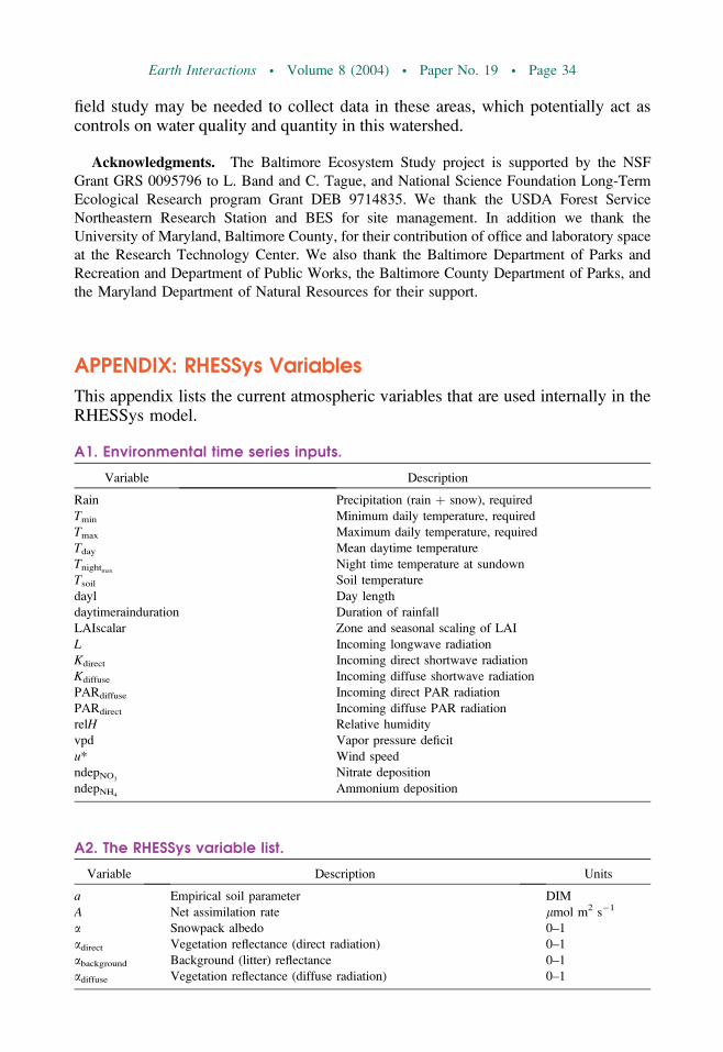
field study may be needed to collect data in these areas, which potentially act ascontrols on water quality and quantity in this watershed.

Acknowledgments. The Baltimore Ecosystem Study project is supported by the NSF

Grant GRS 0095796 to L. Band and C. Tague, and National Science Foundation Long-Term

Ecological Research program Grant DEB 9714835. We thank the USDA Forest Service

Northeastern Research Station and BES for site management. In addition we thank the

University of Maryland, Baltimore County, for their contribution of office and laboratory space

at the Research Technology Center. We also thank the Baltimore Department of Parks and

Recreation and Department of Public Works, the Baltimore County Department of Parks, and

the Maryland Department of Natural Resources for their support.

APPENDIX: RHESSys Variables

This appendix lists the current atmospheric variables that are used internally in theRHESSys model.

A1. Environmental time series inputs.

Variable Description

Rain Precipitation (rain þ snow), required

Tmin Minimum daily temperature, required

Tmax Maximum daily temperature, required

Tday Mean daytime temperature

TnightmaxNight time temperature at sundown

Tsoil Soil temperature

dayl Day length

daytimerainduration Duration of rainfall

LAIscalar Zone and seasonal scaling of LAI

L Incoming longwave radiation

Kdirect Incoming direct shortwave radiation

Kdiffuse Incoming diffuse shortwave radiation

PARdiffuse Incoming direct PAR radiation

PARdirect Incoming diffuse PAR radiation

relH Relative humidity

vpd Vapor pressure deficit

u* Wind speed

ndepNO3Nitrate deposition

ndepNH4Ammonium deposition

A2. The RHESSys variable list.

Variable Description Units

a Empirical soil parameter DIM

A Net assimilation rate lmol m2 s�1

a Snowpack albedo 0–1

adirect Vegetation reflectance (direct radiation) 0–1

abackground Background (litter) reflectance 0–1

adiffuse Vegetation reflectance (diffuse radiation) 0–1


A2. (Continued)


Asunlit Sunlit assimilation rate lmol m2 s�1

Ashaded Shaded assimilation rate lmol m2 s�1

agsurf Empirical moss parameter DIM

ai Area for patch m2

Age Age of snowpack surface Days

alloccrootc.stemc Ratio of carbon allocated to coarse root and stem Ratio

alloclivewood.woodc Ratio of carbon allocated to live and dead wood Ratio

APARdirect Absorbed photosynthetically active direct radiation lmol m2 day�1

APARdiffuse Absorbed photosynthetically active diffuse radiation lmol m2 day�1

ar Upslope contributing area m2

b Pore size index DIM

b Empirical soil parameter DIM

bMT Empirical temperature melt coefficient DIM

b Species specific empirical constant DIM

c Pore disconnectedness index DIM

c Empirical soil parameter DIM

Csoil Soil carbon mass kgC m�2

cpool:to:leafc Total amount of carbon allocated to leaves kg m2 day�1

cpool:to:leafcstore Carbon to be allocated to leaves during the next leaf out period kg m2

Csurf Surface conductance for soil m day�1

CF Cloud fraction %

CI Canopy interception m

CIlitter Litter interception m

cn Vegetation specific wind attenuation coefficient 0 � 1

CO2 Atmospheric carbon dioxide concentration ppm

cprain Specific rain interception capacity m

cpsnow Specific snow interception capacity m

cpwater Heat capacity of water kJ kg K�1

cs.dead.stem Heartwood stem carbon store kg m2

cs.live.stem Sapwood stem carbon store kg m2

d Empirical soil parameter DIM

d0 Zero plane displacement m

Dday Day length s

Drain Daytime rain duration s

du Understory zero plane displacement m

dayl Daylength s

daytimerainduration Duration of rainfall s

detS Surface detention storage m

E Total daily evaporation m day�1

E Evaporation m day�1

ea Atmospheric vapor pressure Pa

essatm Atmospheric emissivity Pa

ETsat Evapotranspiration from the saturated zone m day�1

ETunsat Evapotranspiration from the unsaturated zone m day�1

extcoef Canopy radiation extinction coefficient 0 � 1

F Fractional canopy cover over the snowpack %

fleaf Fraction of assimilate allocated to leaves %

froot Fraction of assimilate allocated to roots %

gpsn Gross daily canopy photosynthesis kgC m2 day�1

GF Gap fraction 0 � 1

grperc Percentage of NPP to growth respiration %

gs Canopy conductance m s�1


A2. (Continued)


gsmax Vegetation type specific maximum conductance m s�1

gsnonvas Nonvascular conductance m s�1

gssunlit Sunlit stomatal conductance m s�1

gsshade Shaded stomatal conductance m s�1

hrCO2Soil (heterotrophic) respiration rate kgC m2 day�1

I Rainfall intensity m day�1

irad Net incoming radiation lmol m2 s�1

k Vegetation-specific Beer’s law extinction coefficient 0 � 1

Kdiffuse Absorbed diffuse shortwave radiation kJ m2 day�1

Kdiffuse0 Incoming diffuse shortwave radiation kJ m2 day�1

Kdirect Absorbed direct shortwave radiation kJ m2 day�1

Kdirect0 Incoming direct shortwave radiation kJ m2 day�1

Ksat0 Saturated hydraulic conductivity at the surface m day�1

Ksats Saturated hydraulic conductivity m day�1

Ksnow Snowpack radiation extinction coeff 0 � 1

Kunsat Vertical unsaturated hydraulic conductivity m day�1

L Longwave radiation kJ m2 day�1

kv Latent heat of vaporization kJ kg�1

kf Latent heat of fusion kJ kg�1

LAIprojshade Shaded projected leaf area index DIM

LAIprojsunlit Sunlit projected leaf area index DIM

litterraincap Maximum litter interception capacity m

livewoodturnover Rate of sapwood to heartwood turnover %

lnc Leaf nitrogen concentration kg(Nleaf/m2)

LWP Leaf water potential MPa

LWPmin.spring Fully open stomata leaf water potential MPa

LWPpredawn Predawn leaf water potential MPa

m Decay rate of hydraulic conductivity with depth DIM

Mrad Radiation melt m day�1

MT Latent and sensible heat melt m day�1

MV Advective melt m day�1

mortality Annual plant mortality rate % yr�1

Ndentrif Denitrification rate kgN m�2 day�1

Nnitrif Nitrification rate kgN m�2 day�1

Nsoil Soil nitrogen mass kgN m2

ndepNO3Atm NO3 deposition kgN m�2 day�1

ndepNH4Atm NH4 deposition kgN m�2 day�1

netpsn Net daily photosynthesis kgN m�2 day�1

nlc Percentage of NPP to be allocated daily %

NH4conc Soil ammonium concentration kgN m�3

NO3decay Parameter: vertical distribution of N in rooting zone DIM

NO3out Total export of nitrate N from patch kgN m�2 day�1

NO3mobile Proportion of soil nitrate that is mobile %

NO3surface Nitrate at top of soil profile kg m�2

NO3.soil Available nitrate in the soil kgN m�2

xa,b Flow width between patch a and b m

p Decay of porosity with depth DIM

P Precipitation m day�1

/ Porosity %

/0 Surface porosity %

pa Atmospheric pressure Pa

PAI Plant area index DIM


A2. (Continued)


PARdirect0 Incoming direct PAR radiation kJ m�2 day�1

PARdiffuse0 Incoming diffuse PAR radiation kJ m�2 day�1

potqexfil Potential exfiltration rate m day�1

ppfdshade Shaded leaf photon flux density lmol m�2 s�1

ppfdsunlit Sunlit leaf photon flux density lmol m�2 s�1

psnactual Photosynthesis (with water, N limitation) kgC m�2 day�1

psnpot Photosynthesis (no water, N limitation) kgC m�2 day�1

qbase Baseflow for the hillslope m day�1

qcap Capillary rise m day�1

qdrain Unsaturated zone drainage m day�1

qinfil Infiltration m day�1

qmelt Snowmelt m day�1

qz Net lateral transport of water from the patch m day�1

q(t)a,b Saturated throughflow m day�1

Rnet Net radiation kJ m�2 day�1

RNO3Maximum denitrification rate kgN m�2 day�1

qwater Density of water kg m�3

rw Species specific empirical constant DIM

rao Overstory resistance s m�1

rau Understory resistance s m�1

rain Incoming precipitation m

RT Rain throughfall m

s Saturation deficit (water) m(water)

S Relative soil moisture content %

S Rooting zone soil wetness %

�s Hillslope mean saturation deficit m

sactive.soil.depth Soil hydrologic depth m

Sc Scattering coefficient 0 � 1

Sfc(z) Relative saturation at field capacity %

Slitter Current water content m

Sp Sorptivity m=ffiffiffiffiffiffiffiday

p

sunsat Soil moisture content of the unsaturation zone m

SED Snowpack energy deficit 8C

SEDmax Maximum energy deficit 8C

�s0 Hillslope mean saturation deficit, w capillary fringe m

r Stefan–Boltzmann constant cal cm�2 day�1 K4

soil.N.avail Total mineral soil N kgN m�2

soil.NH4 Soil ammonia kgN m�2

soil.NO3 Soil nitrate kgN m�2

soil.sminn Mineralized soil nitrogen kgN m�2

surfNO3 Nitrate in surface detention store kg m�2

swa Stem wood equivalent area DIM

Trp Total transpiration m day�1

Tair Mean daily temperature 8C

Tavg Average daily temperature 8C

td Precipitation duration days

Tday Mean daytime temperature 8C

Te Mean hillslope transmissivity m day�1

Tmax Maximum daily temperature 8C

Tmaxsnow Maximum temperature at which snow can occur 8C

Tmin Minimum daily temperature 8C


References

Aber, J. D., and J. M. Melillo, 1991: Terrestrial Ecosystems. Saunders College Publishing,

429 pp.

Ambroise, B., K. J. Beven, and J. Freer, 1996: Towards a generalisation of the topmodel con-

cepts: Topographic indices of hydrological similarity.Water Resour. Res., 32, 2135–2145.Band, L., 1993: Effect of land surface representation on forest water and carbon budgets. J.

Hydrol., 150, 749–772.——, D. Peterson, S. Running, J. Coughlan, R. Lammers, J. Dungan, and R. Nemani, 1991:

Forest ecosystem processes at the watershed scale: Basis for distributed simulation. Ecol.

Modell., 56, 171–196.——, J. Patterson, R. Nemani, and S. Running, 1993: Forest ecosystem processes at the

watershed scale: Incorporating hillslope hydrology. Agric. For. Meteor., 63, 93–126.

A2. (Continued)


Tminrain Minimum temperature at which rain can occur 8C

TnightmaxNight time temperature at sundown 8C

To Local transmissivity m day�1

tp Time to ponding days

Tsoil Soil temperature 8C

tscale Temperature scalar multiplier 0�1

TF Net throughfall from canopy layers m day�1

h Soil moisture %

h0 Initial soil moisture content %

hfc Field capacity %

�I Current interception storage m

�ImaxSpecific rain capacity m

�I0 Relative interception storage m

�noon Solar angle at noon deg

hunsat Unsaturated soil moisture %

totalmr Total canopy maintenance respiration kgC m�2 day�1

Tr Transmissivity m day�1

u* Wind speed m s�1

u* Friction velocity m s�1

uo Wind-speed at top of canopy m s�1

uae Air entry pressure m

�w Mean hillslope wetness index DIM

wi Local wetness index DIM

wscale Soil moisture scalar multiplier 0�1

z Saturation depth m

zo Overstory canopy height m

zsc Screen height m

zsoil Soil depth m

zu Understory canopy height m

zzone Zone elevation m

zo0 Roughness length m

zoo Understory zero plane displacement m

zou Understory roughness length m


——, C. Tague, S. Brun, D. Tenenbaum, and R. Fernandes, 2000: Modelling watersheds as

spatial object hierarchies: Structure and dynamics. Trans. Geogr. Info. Syst., 4, 181–196.——, ——, and P. Groffman, 2001: Forest ecosystem processes at the watershed scale:

Hydrological and ecological controls of nitrogen export. Hydrol. Processes, 15, 2013–2028.

Baron, J. S., M. D. Hartman, T. G. F. Kittel, L. E. Band, D. S. Ojima, and R. B. Lammers,

1998: Effects of land cover, water redistribution, and temperature on ecosystem processes

in the South Platte basin. Ecol. Appl., 8, 1037–1051.Beven, K., and M. Kirkby, 1979: A physically-based variable contributing area model of basin

hydrology. Hydrol. Sci. Bull., 24, 43–69.Chen, J., P. M. Rich, S. Gower, J. Norman, and S. Plummer, 1997: Leaf area index of boreal

forests: Theory, techniques, and measurements. J. Geophys. Res., 102, 29 429–29 444.

——, J. Liu, J. Cihlar, and M. Goulden, 1999: Daily canopy photosynthesis model through

temporal and spatial scaling for remote sensing applications. Ecol. Modell., 124, 99–119.Clapp, R., and G. Hornberger, 1978: Empirical equations for some soil hydraulic properties.

Water. Resour. Res., 14, 601–604.Coughlan, J., and S. Running, 1997: Regional ecosystem simulation: A general model for

simulating snow accumulation and melt in mountainous terrain. Landscape Ecol., 12,119–136.

Creed, I., and L. Band, 1998: Exploring functional similarity in the export of nitrate-n from

forested catchments: A mechanistic modeling approach. Water Resour. Res., 34, 3079–3093.

——, C. Tague, R. Swanson, and R. L. Rothwell, 2000: The potential impacts of harvesting on

the hydrologic dynamics of boreal watersheds. Proc. American Geophysical Union 2000Spring Meeting, Washington, D. C., Amer. Geophys. Union.

Croley, T., 1989: Veritable evaporation modeling on the Laurentian Great Lakes. WaterResour. Res., 25, 781–792.

Daly, C., R. Neilson, and D. Phillips, 1994: A statistical–topographic model for mapping

climatological precipitation over mountainous terrain. J. Appl. Meteor., 33, 140–157.Dickenson, R., M. Shaikh, R. Bryant, and L. Graumlich, 1998: Interactive canopies for a

climate model. J. Climate, 11, 2823–2836.Dingman, S., 1994: Physical Hydrology. Prentice Hall, 646 pp.

Dunne, T., and L. Leopold, 1979: Water in Environmental Planning. W. H. Freeman and

Company, 818 pp.

Eagleson, P., 1978: Climate, soil and vegetation. 3. A simplified model of soil moisture

movement in the liquid phase. Water Resour. Res., 14, 722–730.Evans, J., and A. Jakeman, 1998: Development of a simple, catchment-scale, rainfall–

evapotranspiration–runoff model. Environ. Modell. Software, 13, 385–393.Farquhar, G., and S. vonCaemmerer, 1982: Modeling photosynthetic response to environ-

mental conditions. Encyclopedia of Plant Physiology, O. Lange et al., Eds., New Series,

Vol. 12B, Springer-Verlag, 549–587.

Gold, A., P. Groffman, K. Addy, D. Kellog, M. Stolt, and A. Rosenblatt, 2001: Landscape

attributes as controls on groundwater nitrate removal capacity of riparian zones. J. Amer.Water Resour. Assoc., 37, 1457–1464.

Green, W., and G. Ampt, 1911: Studies on soil physics. 1: The flow of air and water through

soils. J. Agric. Sci., 4, 1–24.Hartman, M., J. Baron, R. Lammers, B. Cline, and L. T. Band, 1999: Simulations of snow

distribution and hydrology in a mountain basin. Water Resour. Res., 35, 1587–1603.Heddeland, I., and D. Lettenmaier, 1995: Hydrological Modeling of Boreal Forest Ecosystems.


Water Resource Series, Vol. 14, Dept. of Civil Engineering, University of Washington,

38 pp.

Jarvis, P., 1976: The interpretations of the variations in leaf water potential and stomatal

conductance found in canopies in the field. Philos. Trans. Roy. Soc. London, B273, 593–610.

Jones, H., 1992: Plants and Microclimate: A Quantitative Approach to Plant Physiology.Cambridge University Press, 452 pp.

Kelliher, F., T. Black, and D. Price, 1986: Estimating the effects of understory removal from a

douglas fir forest using a two-layer canopy evapotranspiration model. Water Resour.Res., 22, 1891–1899.

Krezek, C., 2001: Climatic regulation of peak flows and their contributing source areas under

natural and disturbed conditions in the carnation creek watershed, Vancouver Island, BC,

Canada. M.S. thesis, University Western Ontario, Plant Science and Environmental

Studies, 255 pp.

Lammers, R., and L. Band, 1990: Automating object descriptions of drainage basins. Comput.Geosci., 16, 787–810.

——, ——, and C. Tague, 1997: Scaling behaviour of watershed processes. Scaling-Up: FromCell to Landscape, P. van Gardingen, G. Foody, and P. Curran, Eds., Cambridge

University Press, 295–317.

Landsberg, J., and R. Waring, 1997: A generalized model of forest productivity using

simplified concepts of radiation-use efficiency, carbon balance and partitioning. For.Ecol. Manage., 95, 209–228.

Laramie, R., and J. Schaake Jr., 1972: Simulation of the continuous snowmelt process. Tech.

Rep. 143, Ralph M. Parsons Laboratory, Massachusetts Institute of Technology,

Cambridge, MA.

Laundrum, L., C. L. Tague, and J. Baron, 2002: Modeling hydrologic and biogeochemical

processes in Loch Vale watershed using the regional hydroecological simulation system

(rhessys). Proc. 36th Annual Geological Society of America, South-Central SectionMeeting, Alpine, TX, Geological Society of America, South-Central Section.

Luce, C., and T. Cundy, 1994: Parameter identification for a runoff model for forest roads.

Water Resour. Res., 30, 1057–1069.Mackay, D., and L. Band, 1997: Forest ecosystem processes at the watershed scale: Dynamic

coupling of distributed hydrology and canopy growth. Hydrol. Proc., 11, 1197–1217.Manley, R., 1977: The soil moisture component of mathematical catchment simulation models.

J. Hydrol., 35, 341–356.McDonnell, J., 1990: A rationale for old water discharge through macropores in a steep humid

catchment. Water Resour. Res., 26, 2821–2832.Medlyn, B. E., and Coauthors, 2001: Stomatal conductance of forest species after long-term

exposure to elevated CO2 concentration: A synthesis. New Phytologist, 149, 247–264.Mitchell, S. W., and F. Csillag, 2000: Does pattern matter? Handling bias, uncertainty, and

stability of predicted vegetation growth in Grasslands National Park, Saskatchewan.

Proc. Fourth Int. Conf. on Integrating GIS and Environmental Modeling (GIS/EM4):Problems, Prospects and Research Needs, Banff, Canada.

Monteith, J., 1965: Evaporation and the environment. Proceedings of the 19th Symposium ofthe Society for Experimental Biology, Cambridge University Press, 205–233.

Nash, I., and I. Sutcliffe, 1970: Streamflow forecasting through conceptual models. J. Hydrol.,10, 282–290.

Norman, J., 1981: Simulation of microclimates. Biometeorology in Integrated Pest Manage-ment, J. Hatfield and I. J. Thomson, Eds., Academic Press, 65–99.


Oke, T., 1987: Boundary Layer Climates. 2d ed. University Press, 450 pp.

Parton, W., A. Mosier, D. Ojima, D. Valentine, D. Schimel, K. Weier, and A. Kulmala, 1996:

Generalized model for N2 and N2O production from nitrification and denitrification.

Global Biogeochem. Cycles, 10, 401–412.Peters, D., J. Buttle, C. Taylor, and B. LaZerte, 1995: Runoff production in a forested, shallow

soil Canadian shield basin. Water Resour. Res., 31, 1291–1304.Phillip, J., 1957: The theory of infiltration: 4. Sorptivity and algebraic infiltration equation.

Soil Sci., 84, 257–264.Quinn, P., K. Beven, P. Chevallier, and O. Planchon, 1991: The prediction of hillslope flow paths

for distributed hydrological modeling using digital terrain models.Hydrol. Proc., 5, 59–79.Refsgaard, J., and B. Storm, 1995: MIKE SHE. Computer Models of Watershed Hydrology, V.

Singh, Ed., Water Resources Publications, 809–846.

Running, S., and J. Coughlan, 1988: A general model of forest ecosystem processes for

regional applications: Hydrologic balance, canopy gas exchange and primary production

processes. Ecol. Modell., 42, 125–154.——, and E. Hunt, 1993: Generalization of a forest ecosystem process model for other biomes,

BIOME-BGC and an application for global-scale models. Scaling PhysiologicalProcesses: Leaf to Globe, J. R. Ehleringer and C. Field, Eds., Academic Press, 141–158.

——, R. Nemani, and R. Hungerfored, 1987: Extrapolation of synoptic meteorological data in

mountainous terrain and its use for simulating forest evapotranspiration and photosyn-

thesis. Can. J. For. Res., 17, 472–483.——, ——, D. L. Peterson, L. E. Band, D. F. Potts, L. L. Pierce, and M. A. Spanner, 1989:

Mapping regional forest evapotranspiration and photosynthesis by coupling satellite data

with ecosystem simulation. Ecology, 70, 1090–1101.Ryan, M. G., 1991: Effects of climate change on plant respiration. Ecol. Appl., 1, 157–167.Tague, C., and L. Band, 2001: Simulating the impact of road construction and forest

harvesting on hydrologic response using rhessys. Earth Surface Processes Landforms,26, 135–151.

——, ——, P. Groffman, and K. Belt, 2000: Spatially distributed modeling of the hydro-

geologic and ecologic controls on nitrogen cycling and nitrate export for a small forested

watersheds. Proc. American Geophysical Union 2000 Spring Meeting,Washington, D. C.,

Amer. Geophys. Union.

Thornton, P., 1998: Regional ecosystem simulation: Combining surface and satellite based

observations to study linkages between terrestrial energy and mass budgets. Ph.D. thesis,

School of Forestry, University of Montana, Missoula, 200 pp.

——, S. Running, and M. White, 1997: Generating surfaces of daily meteorological variables

over large regions of complex terrain. J. Hydrol., 190, 214–251.vanGenuchten, M., and D. Nielsen, 1984: On describing and predicting the hydraulic

properties of unsaturated soils. Ann. Geophys., 3, 615–628.Vertessy, R., T. Hatton, P. O’Shaughnessy, and M. Jayasuriya, 1993: Predicting water yield

from a mountain ash forest catchment using a terrain analysis based catchment model. J.Hydrol., 150, 665–700.

Walko, R., and Coauthors, 2000: Coupled atmosphere–biophysics–hydrology models for

environmental modeling. J. Appl. Meteor., 39, 931–944.Waring, R., and S. Running, 1998: Forest Ecosystems: Analysis at Multiple Scales. Academic

Press, 370 pp.

Watson, F., R. Vertessy, and R. Grayson, 1999: Large scale modelling of forest hydrological

processes and their long term effect on water yield. Hydrol. Processes, 13, 689–700.Webster, K., I. Creed, and C. Tague, 2001: Modeling n export from the Noland Divide


watershed: The importance of climate on nitrate-n production and transport. GordonResearch Conference on Forested Catchments: Hydrological, Geochemical, andBiological Processes, Andover, NH.

Wemple, B. C., J. Jones, and G. Grant, 1996: Channel network extension by logging roads in

two basins, Western Cascades, Oregon. Water Resour. Bull., 32, 1195–1207.White, M., P. Thornton, and S. Running, 1997: A continental phenology model for monitoring

vegetation responses to interannual climatic variability. Global Biogeochem. Cycles, 11,217–234.

Wigmosta, M., L. Vail, and D. Lettenmaier, 1994: Distributed hydrology–vegetation model for

complex terrain. Water Resour. Res., 30, 1665–1679.Williams, T., and L. Flanagan, 1997: Effect of changes in water content on photosynthesis,

transpiration and discrimination agains 13CO2 and C18O16O in pleurozium and

sphagnum. Oecologica, 108, 34–46.Zheng, D., E. Hunt, and S. Running, 1993: A daily soil temperature model based on air

temperature and precipitation for continental applications. Climate Res., 2, 183–191.

Earth Interactions is published jointly by the American Meteorological Society, the American Geophysical

Union, and the Association of American Geographers. Permission to use figures, tables, and brief excerpts

from this journal in scientific and educational works it hereby granted provided that the source is

acknowledged. Any use of material in this journal that is determined to be ‘‘fair use’’ under Section 107 or that

satisfies the conditions specified in Section 108 of the U.S. Copyright Law (17 USC, as revised by P.IL. 94-

553) does not require the publishers’ permission. For permission for any other form of copying, contact one of

the copublishing societies.


rhessys: regional hydro-ecologic simulation … current version of rhessys continues to follow the...

Documents