rheology of solid polymers igor emri · rheology of solid polymers igor emri ... university of...
TRANSCRIPT

I. Emri, Rheology Reviews 2005, pp 49 - 100.
© The British Society of Rheology, 2005 (http://www.bsr.org.uk) 49
RHEOLOGY OF SOLID POLYMERS
Igor Emri
Center for Experimental Mechanics, Faculty of Mechanical Engineering
University of Ljubljana, 1125 Ljubljana (SLOVENIA)
ABSTRACT
The mechanical properties of solid polymeric materials quite generally depend
on time, i.e., on whether they are deformed rapidly or slowly. The time dependence is
often remarkably large. The complete description of the mechanical properties of a
polymeric material commonly requires that they be traced through 10, 15, or even 20
decades of time. The class of polymeric materials referred to as thermo-rheologically
and/or piezo-rheologically simple materials allows use of the superposition of the
effects of time and temperature and/or time and pressure in such materials as a
convenient means for extending the experimental time scale.
This paper presents a critical review of models proposed to describe the effect
of temperature and/or pressure on time-dependent thermo-rheologically and/or piezo-
rheologically simple polymeric materials. The emphasis here is on the theoretical
aspects, although experimental results are used as illustrations wherever appropriate.
KEYWORDS: Excess enthalpy, excess entropy, FMT model, free volume, glass
transitions, pressure effects, rate processes, shift functions, temperature effects, time-
temperature-pressure superposition, WLF model
1. INTRODUCTION
Polymeric materials exhibit time-dependent mechanical properties that can
profoundly affect the performance of polymer products. The degree of change in the
mechanical properties of polymeric materials over time depends on many factors.
These are primarily the temperature, pressure, humidity, and stress conditions to which
the material is subjected during its manufacture and during its application. Therefore,
processing parameters, like pressure and temperature, play an important role in
determining the quality of parts made by injection moulding, compression moulding,
extrusion, etc. Unsuitable processing conditions may cause parts to warp or crack.
These phenomena can occur in manufactured articles even in the absence of any
mechanical loading, in particular, in the presence of high-modulus fillers. Explosions
(detonations) represent special cases entailing extremely high temperatures and
pressures.

I. Emri, Rheology Reviews 2005, pp 49 - 100.
© The British Society of Rheology, 2005 (http://www.bsr.org.uk) 50
The mechanical behaviour of polymeric materials is generally characterized in
terms of their time-dependent properties in shear or in simple tension. The time
dependence of their bulk properties is almost universally neglected (see, e.g., Kralj et
al., [1]). The effect of temperature on the shear and tensile properties of polymeric
materials has been fairly well understood since about the forties of the last century. By
contrast, little effort went into the determination of their time-dependent bulk
properties and – after initial years of activity – research on the effect of pressure lay
effectively dormant. This was probably due mainly to the difficulty of making precise
measurements at rather small volume deformations. The materials used in current
applications simply did not appear to require a deeper understanding of the time
dependence of their bulk properties and of the effect of pressure on their time-
dependent shear properties to warrant exerting the exacting effort required. This
situation has now changed. The demand for sustainable development1 requires
optimization of the functional and mechanical properties of new multi-component
systems such as composite and hybrid materials, structural elements, and entire
structures. Optimization of material use requires a much deeper understanding of the
effect that temperature and pressure exert on the time dependence of the bulk as well
as the shear properties of the constituents of these materials than is currently available.
Our primary focus in this paper is the effect of pressure. However, we also
review the effect of temperature, essentially as necessary background. In particular, we
examine whether and in what manner the effects of time and temperature, respectively,
those of time and pressure, may be assumed to superpose. In what follows we shall
therefore pay attention largely to time-temperature and/or time-pressure relations.
Measurements of a linear viscoelastic response function are, however, quite often
reported as a function of frequency. This may be either the cycles/second frequency,
f , or the radian frequency, 2 fω π= . Because ln lnt f≈ − , time and frequency are,
mutatis mutandis, equivalent in considerations of the effects of temperature and/or
pressure.
1.1 Thermo- and piezo-rheological simplicity – shift functions.
For a special class of polymeric materials, primarily single-phase, single-
transition amorphous homopolymers and random copolymers, it is possible to
establish temperature and/or pressure shift functions that ‘collapse’, as it were, the
two-dimensional contour plots into a simple graph of the chosen response function as a
function of the logarithmic time, usually shown as log t , or the logarithmic frequency,
shown as logω or log f , recorded at a reference temperature, 0T , or pressure, 0P .
Such materials are referred to as thermo-rheologically and/or piezo-rheologically
simple materials.
1 Sustainable development aims at preserving, for the benefit of future generations, the
environment and the natural resources culled from it without lowering currently excepted
standards of living.

I. Emri, Rheology Reviews 2005, pp 49 - 100.
© The British Society of Rheology, 2005 (http://www.bsr.org.uk) 51
Thermo-rheological simplicity requires that all response times (i.e., all
relaxation or retardation times, see Tschoegl [2], p. 86), depend equally on
temperature. This is expressed by the temperature shift function:
0
0
( )( )
( )
iT
i
Ta T
T
τ
τ= , 1, 2,....i = ………. (1)
An analogous requirement applies to piezo-rheological simplicity. This
demands that all that all response times depend equally on pressure and is expressed
by the pressure shift function:
0
0
( )( )
( )
iP
i
Pa T
P
τ
τ= , 1, 2,....i = ………. (2)
Thermo-rheologically simple materials allow, by definition, time-temperature
superposition, Gross [3, 4], i.e., the shifting of isothermal segments into superposition
to generate a master curve, thereby extending the time scale beyond the range that
could normally be covered in a single experiment. Figure 1a shows a schematic
illustrating this procedure.
Fillers and Tschoegl [5], and Moonan and Tschoegl [6] showed that piezo-
rheologically simple materials permit analogous, time-pressure superposition, i.e., the
shifting of isobaric segments in a similar manner. Because of the equivalence of time
and frequency, shifting of isothermal (or isobaric) segments along the logarithmic
frequency axis applies just as it applies to shifting along the logarithmic time axis.
Figure 1: (a) Shifting isothermal segments into a master curve; (b) two
master curves at different temperatures.
(a)
log t/aT
log aT
T > T0
T T0
log t/aT
T1
T2
T3
(b)
aT1
aT3 aT2
T0 <T1 <T2 <T3
T0
log
(
)G
t
I. Emri, Rheology Reviews 2005, pp 49 - 100.
© The British Society of Rheology, 2005 (http://www.bsr.org.uk) 52
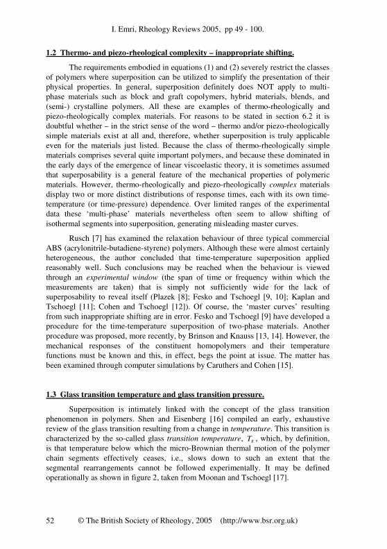
1.2 Thermo- and piezo-rheological complexity – inappropriate shifting.
The requirements embodied in equations (1) and (2) severely restrict the classes
of polymers where superposition can be utilized to simplify the presentation of their
physical properties. In general, superposition definitely does NOT apply to multi-
phase materials such as block and graft copolymers, hybrid materials, blends, and
(semi-) crystalline polymers. All these are examples of thermo-rheologically and
piezo-rheologically complex materials. For reasons to be stated in section 6.2 it is
doubtful whether – in the strict sense of the word – thermo and/or piezo-rheologically
simple materials exist at all and, therefore, whether superposition is truly applicable
even for the materials just listed. Because the class of thermo-rheologically simple
materials comprises several quite important polymers, and because these dominated in
the early days of the emergence of linear viscoelastic theory, it is sometimes assumed
that superposability is a general feature of the mechanical properties of polymeric
materials. However, thermo-rheologically and piezo-rheologically complex materials
display two or more distinct distributions of response times, each with its own time-
temperature (or time-pressure) dependence. Over limited ranges of the experimental
data these ‘multi-phase’ materials nevertheless often seem to allow shifting of
isothermal segments into superposition, generating misleading master curves.
Rusch [7] has examined the relaxation behaviour of three typical commercial
ABS (acrylonitrile-butadiene-styrene) polymers. Although these were almost certainly
heterogeneous, the author concluded that time-temperature superposition applied
reasonably well. Such conclusions may be reached when the behaviour is viewed
through an experimental window (the span of time or frequency within which the
measurements are taken) that is simply not sufficiently wide for the lack of
superposability to reveal itself (Plazek [8]; Fesko and Tschoegl [9, 10]; Kaplan and
Tschoegl [11]; Cohen and Tschoegl [12]). Of course, the ‘master curves’ resulting
from such inappropriate shifting are in error. Fesko and Tschoegl [9] have developed a
procedure for the time-temperature superposition of two-phase materials. Another
procedure was proposed, more recently, by Brinson and Knauss [13, 14]. However, the
mechanical responses of the constituent homopolymers and their temperature
functions must be known and this, in effect, begs the point at issue. The matter has
been examined through computer simulations by Caruthers and Cohen [15].
1.3 Glass transition temperature and glass transition pressure.
Superposition is intimately linked with the concept of the glass transition
phenomenon in polymers. Shen and Eisenberg [16] compiled an early, exhaustive
review of the glass transition resulting from a change in temperature. This transition is
characterized by the so-called glass transition temperature, gT , which, by definition,
is that temperature below which the micro-Brownian thermal motion of the polymer
chain segments effectively ceases, i.e., slows down to such an extent that the
segmental rearrangements cannot be followed experimentally. It may be defined
operationally as shown in figure 2, taken from Moonan and Tschoegl [17].

I. Emri, Rheology Reviews 2005, pp 49 - 100.
© The British Society of Rheology, 2005 (http://www.bsr.org.uk) 53
The figure shows gT obtained from the intersection of a plot of the specific
volume against the temperature, here for two rubbers having the same gT . As
determined experimentally, the glass transition temperature is a kinetic phenomenon
that, however, shows many of the formal aspects of a second-order thermodynamic
phase transition.
Below gT the polymer is not in equilibrium, metastable or otherwise. A certain
amount of entropy is ‘frozen in’ as a consequence of the tremendous loss of chain
mobility that prevents the detection of segmental rearrangements on any finite
experimental time scale. Thus, Nernst’s heat theorem (see, e.g., Tschoegl [18], p. 47),
which requires the entropy to vanish at the absolute zero of temperature, is not obeyed.
DiMarzio and Gibbs [18, 21, 22] have shown that it is possible to postulate the
existence in polymers of a second-order thermodynamic transition temperature, 2T ,
that could, however, be reached only by an infinitely slow cooling process. For
reasons to be stated in section 2.7 we shall designate this temperature as the
‘threshold’ temperature and assign the symbol LT to it. The glass transition
temperature depends on pressure, and this has been noted by several authors (see, e.g.,
Paterson [26], Bianchi [27]).
In analogy to the glass transition temperature, ( )gT P , there exists also a glass
transition pressure, ( )gP T , above which the micro-Brownian motion of the polymer
chain segments ceases. Above gP a polymer is again not in thermodynamic
equilibrium for the same reason that is not in equilibrium below gT . One may
postulate that in polymers there exists also a second-order thermodynamic phase
transition pressure, 2P (or LP ), but nothing seems to be known about it at this time,
except its existence. Temperature would presumably affect the glass transition
Figure 2: Operational definition of Tg
0.54
0.53
0.52
0.51
0.50
0.49
Sp
ec
ific
Vo
lum
e [
mk
g x
10
]3
-13
Temperature [ C] º
-80 -40 -22 40 80
Hypalon 40
Viton B
0.5 C/min.º
0.89
0.87
0.85
0.83
0.81
I. Emri, Rheology Reviews 2005, pp 49 - 100.
© The British Society of Rheology, 2005 (http://www.bsr.org.uk) 54
pressure but data on this phenomenon also appear to be lacking. Being kinetic rather
than thermodynamic phenomena, the glass transitions depend on the time rate at which
they are determined. They are actually narrow ranges rather then specific temperatures
or pressures. Superposition requires that the material be in thermal and mechanical
equilibrium. In order to reach the equilibrium in a relatively short period of time,
material must therefore be above the glass transition temperature, gT , and/or below the
glass transition pressure, gP .
1.4 Purpose and scope of the article.
Despite the reservations expressed in the previous sections, superposition has
been and is being used widely. The literature on the effect of temperature on the
mechanical properties of polymeric materials is extensive. That on the effect of
pressure is less so. This article presents a review of what has been done to date in
modelling temperature and/or pressure shift functions for polymeric materials in
equilibrium with respect to temperature and pressure. Two papers concerned solely
with the effect of pressure on the viscosity of non-polymeric liquids, e.g., Matheson
[28], have not been reviewed.
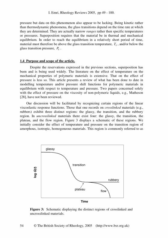
Our discussion will be facilitated by recognizing certain regions of the linear
viscoelastic response functions. Those that one records on crosslinked materials (e.g.,
rubbers) exhibit three distinct regions: the glassy, the transition, and the rubbery
region. In uncrosslinked materials there exist four: the glassy, the transition, the
plateau, and the flow region. Figure 3 displays a schematic of these regions. We
initially consider the effect of temperature and pressure on the transition region of
amorphous, isotropic, homogeneous materials. This region is commonly referred to as
Figure 3: Schematic displaying the distinct regions of crosslinked and
uncrosslinked materials.
glassy
transition
rubbery
Time
log
()
Gt
plateauflow

I. Emri, Rheology Reviews 2005, pp 49 - 100.
© The British Society of Rheology, 2005 (http://www.bsr.org.uk) 55
the ‘main’ transition region to distinguish it from possible other transitions (see section
6.2. The scope will be widened in sections 6, 7, and 8 to include the other regions of
the linear viscoelastic response. We shall consider primarily deformation in shear.
Brief reference will be made to other types of deformation in section 9, and to
anisotropic materials in section 10. In sections 2, 3, and 4 we will introduce various
models describing the effect of temperature and pressure on the mechanical properties
of thermo- and/or piezo-rheologically simple polymeric materials. Each section will
contain a critique of these models. These critiques will be deferred, however, until the
models in each section have all been introduced. We shall further attempt also to point
out – to the best of our understanding – areas where information on the effect of
temperature or pressure on the mechanical properties of thermo- and/or piezo-
rheologically simple materials is currently lacking.
2. MODELLING THE EFFECT OF TEMPERATURE
The effect of temperature on the time-dependent mechanical properties of
polymers is relatively well understood although a number of problems remain open.
Above gT it is generally modeled by the well-known WLF equation, named after its
originators, Williams, Landel, and Ferry. We review the derivation and properties of
this equation as necessary background to our discussion of the effect of pressure. The
WLF equation is concerned with the relaxation or retardation behaviour arising from
the micro-Brownian (or segmental, or backbone) motion of the polymer chains. It has
been derived from consideration of the fractional free volume. However, equations of
the same form have been proposed also by considering the relaxation or retardation
process as the physical counterpart of a chemical reaction, or by considering changes
in the excess (configurational) entropy2, or in the excess enthalpy. While all these
approaches lead to equations of the same form, the empirically obtained parameters of
the equation are interpreted differently.
2.1 The Doolittle equation.
Many theories for modelling the effect of thermodynamic parameters such as
temperature or pressure on the time-dependent behaviour of polymers are based on the
free-volume concept. Doolittle and Doolittle [29] introduced this concept in their work
on the viscosity of liquids. They assumed that the change in viscosity depends on the
distribution of molecule-size holes in the fluid. The sum of these holes represents the
free-volume, which directly affects the mobility of the liquid molecules. Doolittle and
Doolittle [29] expressed this in their semi-empirical expression for the viscosity,η , of
liquids:
2 The excess (configurational) entropy may be defined as the difference between the
(configurational) entropy of the polymer above the glass transition temperature and that of the
glass in a hypothetical reference state from which, even in principle, no more of the property
can be lost due to relaxational processes, Chang et al. [35].

I. Emri, Rheology Reviews 2005, pp 49 - 100.
© The British Society of Rheology, 2005 (http://www.bsr.org.uk) 56
1exp exp exp 1
f
f f
V VVA B A B A B
V V f
φη−
= = = −
. ………. (3)
Here, A and B are empirical material constants, Vφ is the occupied volume (i.e., the
volume occupied by the molecules of the liquid), and fV is the free volume. This is the
unoccupied intermolecular space available for molecular motion. It can also be viewed
as the ‘excess’ volume, i.e., the volume that exceeds the occupied volume. Hence, the
total macroscopic volume is fV V Vφ= + , and /ff V V= called the fractional free
volume. Figure 4 illustrates these concepts schematically. Although these concepts
cannot be formulated rigorously, they make intuitive sense. Temperature affects the
free volume. In equation (3), η and f represent the viscosity and the fractional free
volume at a given temperature, T. Letting 0η , and 0f be the same quantities at a
conveniently chosen reference temperature, 0T , leads to the viscosity ratio:
0 0
1 1exp B
f f
η
η
= −
. ………. (4)
The Doolittle equation originally referred to liquids consisting of small
molecules. Williams et al. [30] adapted it for use with polymers by modifying the
Rouse theory of the behaviour of polymers in infinitely dilute solution to the behaviour
of polymers in bulk, Ferry [31], p. 225. On the basis of this approach they let:
0 0
( ) ( )
( ) ( )
f i
f i
T T
T T
η τ
η τ= or
0 0
f i
f i
η τ
η τ= , ………. (5)
where fη is the steady-state viscosity and iτ is any relaxation time at the same
Figure 4: Volume-temperature diagram of an amorphous polymer.

I. Emri, Rheology Reviews 2005, pp 49 - 100.
© The British Society of Rheology, 2005 (http://www.bsr.org.uk) 57
temperature, T . Further, 0fη and i0τ are the same quantities at the reference
temperature, 0T . Making use of this proportionality, one may define a temperature
shift factor, Ta , as an abbreviation for the temperature shift function, 0( )Ta T , to yield:
0 0
1 1exp
Ta B
f f
τ
τ
= = −
. ……….(6)
If another temperature, say, the glass transition temperature, gT , is chosen as
the reference temperature, we have:
1 1exp
T
g g
a Bf f
τ
τ
= = −
, ……….(7)
where gf is the fractional free volume at gT .
In logarithmic form equation (6) becomes:
0 0
1 1 1 1log
2.303 ( ) ( ) 2.303T
B Ba
f T f T f f
= − = −
, ………. (8)
where log Ta is the distance required to bring (shift) data recorded at the temperature,
T , into superposition with data recorded at the reference temperature, 0T , along the
logarithmic time axis (cf. figure 1). Equation (8) is the starting point for the
temperature shift functions that are based on the free volume concept. In sections 3
and 4 we will show that equations of the same form can serve to model the effect of
pressure, and that of both pressure and temperature.
2.2 The Williams-Landel-Ferry (WLF) model.
Williams et al. [30] modelled the effect of temperature on the mechanical
properties of amorphous homopolymers or random copolymers by considering that the
fractional free volume of such polymers increases linearly with temperature. They thus
let:
0 0( )ff f T Tα= + − , ………. (9)
where fα is the expansivity (i.e., the isobaric cubic thermal expansion coefficient) of
the fractional free volume (cf. figure 4). Substitution of equation (9) into equation (8)
leads to:
0 0
0 0
( / 2.303 )( )log
/T
f
B f T Ta
f T Tα
−= −
+ − . ……….(10)
This is usually used in the form:
0
1 0
0
2 0
( )log
T
c T Ta
c T T
−= −
+ −, ………. (11)

I. Emri, Rheology Reviews 2005, pp 49 - 100.
© The British Society of Rheology, 2005 (http://www.bsr.org.uk) 58
where:
0
1 0/ 2.303c B f= ………. (12)
and
0
2 0 /f
c f α= . ………. (13)
Equation (11) is the WLF equation. The superscript 0 refers the parameters of the
equation to the reference temperature, 0T . If a different reference temperature, say, rT ,
is chosen, the constants must be changed using the symmetric relations:
0
2 2 0
r
rc c T T= + − , ………. (14)
and
0 0
1 2 1 2
r rc c c c= . ………. (15)
The product, 1 2c c , is independent of the reference temperature and may
therefore be written without superscripts. Referred to the glass transition temperature,
the WLF equation becomes:
1
2
( )log
g
g
T g
g
c T Ta
c T T
−= −
+ −, ………. (16)
where now, however:
1 / 2.303g
gc B f= ………. (17)
and
2 /g
g fc f α= , ………. (18)
with gf as the fractional free volume at the glass transition temperature.
The constants, 1c and 2c , are found experimentally by shifting isothermal
segments of the response function into superposition along the logarithmic abscissa to
yield a ‘master curve’ as illustrated in figure 1a. Figure 1b shows master curves at the
reference temperature, 0T , and at the experimental temperature, T . The constants are
found from the slope and the intercept of a straight line through a plot of log TT a∆
vs. T∆ , Ferry [31], p. 274. The numerical procedure for calculating the constants is
presented in the Appendix A.
Williams et al. [30] also proposed a ‘universal’ form of the WLF equation
having a single adjustable parameter, ST . This form:
8.86( )log
101.6
g
T
g
T Ta
T T
−= −
+ −, ………. (19)

I. Emri, Rheology Reviews 2005, pp 49 - 100.
© The British Society of Rheology, 2005 (http://www.bsr.org.uk) 59
has been found not to be truly ‘universal’ even though it applies reasonably well to
many polymeric materials, see, e.g., Schwarzl and Zahradnik [32]. It should therefore
be used only as a last resort when the constants, 1c and 2c , are not available.
It is of interest to obtain the molecular parameters contained in equations (12)
and (13). However, there are only two known empirical parameters, the shift
constants, 1c and 2c , available for the determination of the three unknown parameters,
B , 0f , and fα . The most common way to deal with this problem has been to assume
that the proportionality factor B is unity, Ferry [31], p. 287. In section 4.3 we adduce
evidence that this assumption cannot be upheld and show how B can be determined
experimentally.
2.3 Bueche’s temperature (BT) model.
Bueche [33] proposed a ‘hole’ theory of the free volume that he considered to
be a modified form of the WLF equation. He derived:
[ ]1 2
2
1log 1
1 ( )T
l
a bb T T
= −
+ −
, ………. (20)
where
2
1
9( * / )
2.303
fLv v
bπ
= , ………. (21)
and
2P
fL
mb
v
α
ρ= . ………. (22)
In these equations, *v is the critical hole volume for molecular rearrangements, fLv is
the free volume per molecular segment at LT , the threshold temperature (see sections
2.5 and 2.7), Pα is the thermal expansion coefficient, m is the molecular weight of
the segment, and ρ is the density. Some of these parameters are not easily
determined.
On the strength of the scanty data available to him then, Bueche concluded that
his equation provided a better approximation at low temperatures while the WLF
equation gave better agreement at higher temperatures. The equation does not seem to
have found many users.
2.4 The Bestul-Chang (BC) model.
Bestul and Chang [34], and Chang et al. [35], modelled the effect of
temperature by considering the (excess) configurational entropy rather than the free
volume. Their logarithmic shift factor takes the form:

I. Emri, Rheology Reviews 2005, pp 49 - 100.
© The British Society of Rheology, 2005 (http://www.bsr.org.uk) 60
1 1log
2.303 ( ) ( )
BC
T
c c g
Ba
S T S T
= −
, ………. (23)
[cf. equation (8)], where ( )cS T and ( )c gS T are the excess entropy of the polymer
above the glass transition temperature, and that of the glass, respectively. Inserting:
( ) ( ) ln ( ) ln( )
g
T
c c g P c g P g
T
S T S T C d T S T C T T= + ∆ = + ∆∫ , ………. (24)
where PC∆ is the difference in the specific heats of the polymer in the rubbery or
plateau region, and the glassy region, respectively, yields:
[ 2.303 ( )]ln( )log
( ) ln( )
BC c g g
T
c g P g
B S T T Ta
S T C T T= −
∆ +. ………. (25)
Since for values near unity ln 1x x −� , the authors let ln( ) ( )g g gT T T T T= − . This
leads to an equation of the form of the WLF equation, where now, however,
12.303 ( )
g BC
c g
Bc
S T= , ………. (26)
and
2
( ).
g c gg
P
T S Tc
C=
∆ ………. (27)
When the experimental temperature, T , is significantly larger than gT , the
approximation used to obtain an equation of the form of the WLF equation may not be
adequate. In that case, however, the logarithm may be expanded to any degree desired,
using:
2 31 1ln ( 1) ( 1) ( 1) , 0 2
2 3x x x x x= − − − + − − < ≤L , ………. (28)
as long as 2g
T T ≤ .
2.5 The Goldstein (GS) model.
Goldstein [36] considered excess enthalpy instead of excess entropy. His model
may be derived in analogy to the BC model by letting the logarithmic shift factor be
given by:
1 1log
2.303 ( ) ( )
GS
T
g
Ba
H T H T
= −
, ………. (29)
where ( )H T and ( )gH T are the excess enthalpy of the polymer above the glass
transition temperature, and that of the glass, respectively. This again leads to a model
of the temperature shift factor that is identical in form with that of the WLF model
except that now:

I. Emri, Rheology Reviews 2005, pp 49 - 100.
© The British Society of Rheology, 2005 (http://www.bsr.org.uk) 61
12.303 ( )
g GS
g
Bc
H T= , ………. (30)
and
2
( ).
gg
P
H Tc
C=
∆ ………. (31)
2.6 The Adam-Gibbs (AG) model.
Goldstein [36] objected to the use of the entropy alone (as in the BC model)
instead of its product with temperature as the principle variable governing glass
formation. The model of Adam and Gibbs [37] is free of this objection. They let:
1 1log
2.303 ( ) ( )
AG
T
c r c r
Ba
TS T T S T
= − −
, ………. (32)
where
( ) ( ) lnc c r P r
S T S T C T T= + ∆ , ………. (33)
is the configurational entropy at the temperature, T , and rT is the reference
temperature [cf. equations (24) and (8)]. PC∆ is the difference in specific heat
between the equilibrium melt and the glass that is considered to be independent of the
temperature. According to DiMarzio and Gibbs [18, 21, 22], although at higher
temperatures the polymer chains are able to assume a large number of configurations,
at their second-order thermodynamic transition temperature, 2T , there is only one (or
at most a very few) configurations available to the backbone. 2T is thus the threshold
temperature below which the relaxation or retardation processes cannot be activated
thermally. We therefore assign to it the symbol LT , taking the subscript L from the
Latin limen, a threshold. The configurational entropy of the glass is thus deemed to
vanish at L
T T= . Setting ( ) 0c L
S T = , equation (33) yields:
( ) lnc r P r L
S T C T T= ∆ . ……….(34)
Substituting this into equation (33) gives ( ) lnc P LS T C T T∆= and equation
(32) thus again leads to an equation of the form of the WLF equation, with:
12.303 ln( )
r AG
P r r L
Bc
C T T T=
∆, ………. (35)
and
[ ]2
ln( )
ln( ) 1 ( ) ln( )
r r r L
r L r r r L
T T Tc
T T T T T T T=
+ + −. ………. (36)

I. Emri, Rheology Reviews 2005, pp 49 - 100.
© The British Society of Rheology, 2005 (http://www.bsr.org.uk) 62
The second parameter is a weak function of the temperature, T , involving the
reference temperature, rT , as well as the threshold temperature, LT . With good
approximation:
[ ]1 ( ) ln( ) 1r r r L
T T T T T+ − � , ………. (37)
and thus:
2
ln( )
1 ln( )
r r r L
r L
r L
T T Tc T T
T T−
+� � . ………. (38)
The second of these equations again follows upon letting ln 1x x −� .
2.7 The rate process (RP) model.
A temperature shift factor identical in form with Ta of the WLF equation may
be derived also from a modification of the Arrhenius equation well known from the
theory of chemical reaction rates. Relaxation (or retardation) may be regarded as a
physical process in which the material is carried from state A into state B. The
response time (relaxation or retardation time) is the time constant for this process. An
increase in temperature shortens the response time because it causes the stress to relax,
or the strain to reach its ultimate value, faster than at a lower temperature.
Consequently, the response time is the reciprocal of the rate at which the physical
change takes place, and is thus akin to the reciprocal of a chemical reaction rate.
Provided that the conventional theory of reaction rates, Kauzmann [38], is applicable
to relaxation and retardation phenomena, one would expect the temperature
dependence of these processes, in analogy to that of a chemical reaction, to be given
by the equation:
exp agA
Tτ
∆=
R, ………. (39)
where ag∆ is the change in the (molar) free enthalpy3 of activation for the process per
degree of temperature, and R is the universal gas constant. The pre-exponential factor
A is considered to be a constant since it is at most a weak function of temperature.
Equation (39) is the physical equivalent of the Arrhenius equation. According
to this equation the relaxation time becomes infinite at the absolute temperature 0T = .
However, an infinite relaxation time implies that the material does not relax. For
polymers, relaxation or retardation behaviour can become effectively impossible well
above 0T = . The backbone motion, i.e., the main chain segmental motion that gives
rise to the response time distribution, ceases below the glass transition temperature,
3 The free enthalpy (cf. Tschoegl [18], p. 56) is also called the Gibbs free energy or Gibbs
potential.

I. Emri, Rheology Reviews 2005, pp 49 - 100.
© The British Society of Rheology, 2005 (http://www.bsr.org.uk) 63
gT . When this is measured at the usual experimental cooling rate of 5 to 15°C/min, it
is about 50°C above 2T . We may therefore set:
50g LT T +� . ………. (40)
Subtracting LT from T modifies equation (39) to allow the response time to become
infinite when LT T= . We then have:
exp( )
a
L
gA
T Tτ
∆=
−R. ………. (41)
Model 1
gc 2
gc
WLF 1 2.303g
gc B f= 2
g
g fc f α=
Bestul-Chang 1 2.303 ( )g
BC c gc B S T= 2 ( )g
g c g Pc T S T C= ∆
Goldstein 1 2.303 ( )g
GS gc B H T= 2 ( )g
g Pc H T C= ∆
Adams-Gibbs 1 2.303 ln( )g
AG P g g Lc B C T T T= ∆ 2
g
g Lc T T= −
Rate Process 1 22.303g g
ac g c= ∆ R 2
g
g Lc T T= −
Table 1: Comparison of the parameters of the temperature
superposition models.
Writing equation (41) for 0τ , dividing it into equation (40), and taking
logarithms leads to:
0
1 1log
2.303
a
T
L L
ga
T T T T
∆= −
− − R. ………. (42)
This may be rearranged to yield equation (11) where now, however,
0
1 0
22.303
agc
c
∆=
R, ………. (43)
and
0
2 0 Lc T T= − . ………. (44)
The former yields an estimate of the apparent molar free enthalpy of activation, while
the latter yields one of LT . Moreover, a plot of log Ta vs. 02 0( )1 c T T+ − yields a
straight line with constant slope:

I. Emri, Rheology Reviews 2005, pp 49 - 100.
© The British Society of Rheology, 2005 (http://www.bsr.org.uk) 64
1 22.303ag c c∆ = R , ………. (45)
as long as these interpretations of the constants 0
1c and 0
2c are accepted.
2.8 Critique of the time-temperature superposition models.
Except for Bueche’s Temperature (BT) model, all other time-temperature
superposition models have the form of the WLF equation or can be reduced to it. They
differ only in the interpretation of the parameters of the equation. The Williams-
Landel-Ferry (WLF), the Bestul-Chang (BC), the Adam-Gibbs (AG), and the
Goldstein (GS) models form a group in that all four consider ‘excess’ quantities. The
rate process (RP) model is, strictly speaking, not based on an excess property although
one might consider LT T− [cf. equation (41)] as the excess of the experimental
temperature, T , over the hypothetical reference temperature, LT .
The BC and AG models are concerned with changes in the configurational
entropy. The coincidence between the WLF and BC and AG models becomes
understandable if one considers that changes in the configurational entropy arisefrom
cooperatively rearranging regions that require free volume in which to move. At
constant pressure the change in enthalpy is given by dH dU PdV= + , where U is the
internal energy. Thus a change in volume underlies also the GS model. Excess (free)
volume, excess entropy, and excess enthalpy are fundamentally related, Eisenberg and
Saito [39], Shen and Eisenberg [16], and Hutchinson and Kovacs [40]. Theoretically,
the excess entropy is an appealing concept. However, volume is much more easily
measured experimentally than entropy or enthalpy, and is plausibly related to
molecular mobility in a simple manner, Ferry [31], p. 285. We note that the WLF
model is the only one that depends on three unknown ‘molecular’ parameters. Since
PC∆ can be determined calorimetrically, all others sport only two.
It would clearly be of interest to decide which of the models is the ‘correct’
one. To do this, one would need to determine separately the molecular parameters in
terms of which the models interpret the constants, 1c and 2c (see table 1).
Unfortunately, only some of those parameters are accessible independently. To see,
nevertheless, how one might distinguish between the models based on the free volume,
the excess entropy, and the excess enthalpy concepts, we first recall that:
f e q gφα α α α α α= − − = ∆� , ………. (46)
and that:
f e q gφκ κ κ κ κ κ= − − = ∆� , ………. (47)
where the subscripts f, e, q, and g refer to the expansivities and the compressibilities of
the free, entire (total), (pseudo-)equilibrium, and glassy volumes, respectively (cf.
figure 4). In the second of these equations we have substituted the (pseudo)-
equilibrium values for those of the entire volume, and the glassy values for those of
the occupied volume. For a justification of the latter, see Moonan and Tschoegl [41].
The change of the free (excess) volume as a function of both temperature and

I. Emri, Rheology Reviews 2005, pp 49 - 100.
© The British Society of Rheology, 2005 (http://www.bsr.org.uk) 65
pressure is given by:
ex ex
ex
V VdV dT dP V dT V dP
T Pα κ
∂ ∂= + = ∆ − ∆
∂ ∂. ………. (48)
Assuming, following Goldstein [36], to whom this treatment is due, that – in
the absence of pressure changes – the free volume is constant, i.e., exdV 0= at and
below the glass transition temperature, we have:
gdT
dP
κ
α
∆=
∆, ………. (49)
if exV determines gT .
For the excess entropy change we have:
2
ex ex P
ex
S S CdS dT dP dT
T P T
α
κ
∂ ∂ ∆ ∆= + = −
∂ ∂ ∆ , ………. (50)
because:
ex PS C
dT dTT T
∂ ∆=
∂, ………. (51)
and
exS
dP VdPP
α∂
= −∆∂
. ………. (52)
But, if we further assume with Goldstein [36] that exdV 0= implies exdS 0= , then:
g
P
dT TV
dP C
α∆=
∆, ………. (53)
if it is exS that determines gT . Goldstein then shows on the basis of a slightly more
involved derivation, that consideration of exH as the determining factor of gT also
leads to equation (53).
Thus, measurements of gdT dP , the change of the glass transition temperature
with pressure, combined with determinations of α∆ , κ∆ , and PC∆ should allow one
to decide whether it is the free volume on the one hand, or the excess entropy or
excess enthalpy on the other hand, that are ‘frozen in’ at and below the glass transition
temperature. So far, measurements have not been made with sufficient accuracy on the
same material in the same laboratory to decide the issue unambiguously. Should a
valid comparison of equations (49) and (53) have decided against the volume as the
governing factor, the question whether it is the excess entropy or the excess enthalpy
that determines the glass transition temperature would still appear to be moot. We
remark that the hypothetical reference temperature of an excess property is property
LT , not gT . The Adam–Gibbs (AG) and the Rate Process (RP) models correctly refer
to LT .

I. Emri, Rheology Reviews 2005, pp 49 - 100.
© The British Society of Rheology, 2005 (http://www.bsr.org.uk) 66
2.9 Measurements as functions of temperature.
Hitherto we have considered isothermal measurements as a function of time, or
of frequency. Measurements are, however, frequently made isochronically, i.e., at
fixed times or at fixed frequencies. Determinations with the forced-oscillation torsion
pendulum are a point in case. The time required to make the measurements must be
short compared with the rate at which the temperature is changed. In practice it is
changed incrementally and the measurements are taken when thermal and mechanical
equilibrium has been reached after each increment. Figure 5 shows a schematic plot of
log ( )G T as function of T.
The temperature at the inflection point, i.e., the inflection temperature, inflT ,
is sometimes considered to be a rough indication of the glass transition temperature,
gT . A plot of, for instance, the shear modulus, as a function of temperature shows
qualitatively the same features as a plot of the same modulus as a function of the
logarithmic time. Yet measurements as a function of temperature at a fixed time or
frequency cannot be brought into superposition by shifting along the T-axis. While the
time shift factor, Ta , and hence also its logarithm, is independent of time or frequency
[cf. equation (11)], the temperature shift factor, T T T ′∆ = − , is evidently a function of
the temperature.
A typical set of ( )G T vs. T curves, for NR (natural rubber), at four isochronal
times 1 2 3 4t t t t< < < is shown in figure 6, taken from Prodan [42].
The shorter the time (or the higher the frequency), the slower is the rate of
response to an increase in temperature. The slope of the log ( )G T vs. T curve
therefore depends both on the steepness of ( )G T and the steepness of Ta at the
particular isochronal time, in accordance with:
Figure 5: A schematic plot of log G(T ) vs. T .
log
(
)G
T
Tinfl
Temperature
t t= 0

I. Emri, Rheology Reviews 2005, pp 49 - 100.
© The British Society of Rheology, 2005 (http://www.bsr.org.uk) 67
loglog ( ) log ( )
log
T
t T tT
t aG T G T
T t a T
∂∂ ∂ = ∂ ∂ ∂
. ………. (54)
Thus, when the temperature response at a fixed time, t, or at a fixed frequency,
ω is given, and Ta is known for any reference temperature rT , the temperature
response at any other fixed time 0t , or fixed frequency, 0ω , can be constructed, but
this must be done point by point. To do this, we must find the temperature, T ′ , to
which the measurement at temperature T must be shifted for a given value of 0t t or
0ω ω .
All this can be understood by the following consideration. Let the parameters of
the WLF equation be known for the polymer under investigation. The shift along the
T-axis is then given by the relations:
2 0 2 0
1 0 1 0
log log
log log
c t t cT
c t t c
ω ω
ω ω
′ ′∆ = =
′ ′− −, ………. (55)
which are obtained from equation (11) by letting 0Ta t t= , or 0ω ω , 0T T T∆− = ,
and then solving for T∆ . A modulus measured at the temperature, T, and at the fixed
time, t (or the fixed frequency, ω) is therefore equivalent to a modulus measured at the
temperature, T T+ ∆ , and at the fixed time, 0t (or fixed frequency, 0ω ). Thus
( ; ) ( ; )G T t G T T tω ω= + ∆ . For each value of the modulus there exists, therefore, a
translation along the temperature axis. However, the amount of the translation is not
constant but varies with T. Equation (55) allows the construction of master curves of
the temperature dependence of a given viscoelastic response function when
measurements at a given fixed time or frequency do not cover the entire desired range.
Figure 6: ( )G T vs. T for four isochronal times, i
t [42].
1
1.5
2
2.5
3
3.5
-30 -25 -20 -15 -10 -5 0 5Temperature [
oC]
log
G(T
) [M
Pa
]
t = 0.16 s
t = 0.40 s
t = 1.00 s
t = 2.51 s
t 1
t 2
t 3
t 4

I. Emri, Rheology Reviews 2005, pp 49 - 100.
© The British Society of Rheology, 2005 (http://www.bsr.org.uk) 68
3. MODELLING THE EFFECT OF PRESSURE
Contrary to the case of the effect of temperature, very little has been reported
on the effect of pressure. Due to the time-dependent nature of polymers, pressure
related material properties, such as the bulk modulus, K, are also functions of time and
are not constant as is often assumed. Furthermore, while K is the reciprocal of the bulk
compliance, B, the time-dependent bulk relaxation modulus, ( )K t , is not the
reciprocal of the time-dependent bulk creep compliance, ( )B t . The two are linked
through the convolution integral:
( ) ( ) lnt
K t u B u d u t−∞
− =∫ , ………. (56)
and are said to be time reciprocal.
Research on the mechanical properties of materials under isotropic pressure
began in the early nineteen forties. P. W. Bridgman4 investigated pressure-induced
changes in the compressibility, viscosity, and thermal conductivity of metals and
nonmetals [43]. First papers on pressure dependence of the glass transition
temperature, gT , appeared in the sixties [27, 33, 44, 46, 47 ].
The effect of pressure on the relaxation behavior of piezo-rheologically simple
polymers is analogous to the effect of temperature on that of thermo-rheologically
simple ones, taking into account that high temperature corresponds to low pressure and
vice versa. In contrast to the effect of temperature, data on the effect of pressure on the
time-dependent properties of polymeric materials are relatively scant because they are
difficult to determine experimentally.
To model the effect of pressure one thus establishes a pressure shift function,
0 ( )Pa P , in analogy to the temperature shift function, ( )0Ta T . Experimentally, ( )0Pa P
is found by shifting isobaric segments of a given response function into superposition.
The feasibility of time-pressure superposition is demonstrated by the experimental
data shown in figure 7, taken from Moonan and Tschoegl [6]. The figure – actually an
instant of time-temperature-pressure superposition to be discussed in section 4.3 –
displays three shear relaxation master curves at different pressures. The curves are
similar in shape and can be shifted into superposition along the logarithmic time axis.
Thus, knowing only one relaxation curve, say, the one at the reference pressure, e.g.,
atmospheric pressure, 0 0.1MPaP = , the other two curves can be predicted if the
pressure shift factor, Pa , is known.
We now turn to the discussion of models for the superposition of the effects of
time (or frequency) and pressure. With the exception of the BP model (see section 3.2)
they can be shown to be based on the equation:
4 P. W. Bridgman: “General survey of certain results in the field of high-pressure
physics”, Nobel Lecture, December 11, (1946)

I. Emri, Rheology Reviews 2005, pp 49 - 100.
© The British Society of Rheology, 2005 (http://www.bsr.org.uk) 69
0 0
1 1 1 1log
2.303 ( ) ( ) 2.303P
B Ba
f P f P f f
= − = −
, ………. (57)
the pressure analogue of equation (8).
3.1 The Ferry-Stratton (FS) model.
The model proposed by Ferry and Stratton [46] (see also McKinney and
Belcher [47], Tribone et al. [48], and Freeman et al. [49]) assumes that the fractional
free volume decreases linearly with pressure. Thus:
0 0( ) ( )f
f P f P Pκ= − − , ………. (58)
where fκ is the isothermal compressibility of the fractional free volume, and P is the
test pressure while 0P is the reference pressure at which 0 0( )f f P= is known.
Introducing equation (58) into equation (57) we obtain the Ferry–Stratton equation as:
0
0 0 0
log2.303 / ( )
P
f
P PBa
f f P Pκ
−=
− − , ………. (59)
or
0
1 0
0
2 0
( )log
P
s P Pa
s P P
−=
+ −, ………. (60)
where:
Figure 7: The effect of pressure on the shear modulus, ( )G t [6].
-0.5
0
0.5
1
1.5
2
2.5
3
3.5
-15 -10 -5 0 5 10 15
0,1 MPa
200 MPa
340 MPa
log
G( t
/a )
[M
Pa ]
log t/ a [s]P
P

I. Emri, Rheology Reviews 2005, pp 49 - 100.
© The British Society of Rheology, 2005 (http://www.bsr.org.uk) 70
0
1
02.303
Bs
f= , ………. (61)
and
0 0
2
f
fs
κ= . ………. (62)
Equations (60) to (62) are the pressure analogues of the corresponding
temperature relations, equations (11) to (13). The equations assume that the
temperature is constant and that fκ does not depend on either T or P.
Equation (60) may be referred to the glass transition pressure, gP by setting:
1
2
( )log
g
g
P g
g
s P Pa
s P P
−=
+ −, ………. (63)
where:
12.303
g
g
Bs
f= , ………. (64)
and
2
gg
f
fs
κ= . ………. (65)
These equations were obtained using:
0
2 0 2
g
gs P s P+ = + , ………. (66)
and
0 0
1 2 1 2
g gs s s s= , ………. (67)
the pressure analogues of equations (14) and (15).
3.2 Bueche’s pressure (BP) model.
Bueche [33] proposed a time-pressure superposition model also. His model is
not based on equation (57). It gives the logarithmic pressure shift factor as:
*
log2.303
P
P va
kT= , ………. (68)
where *v is again the critical hole volume [cf. section 2.3], and k is Boltzmann’s
constant. Bueche considered his model to be no more than a useful approximation.
I. Emri, Rheology Reviews 2005, pp 49 - 100.
© The British Society of Rheology, 2005 (http://www.bsr.org.uk) 71
3.3 The O’Reilly (OR) model.
O’Reilly [50] derived his model from the observation (Ferry [31], p. 293,
Tribone et al. [48], Freeman et al. [49]) that the pressure dependence of the shift
factor, Pa , can be described by the simple exponential relation:
0exp ( )Pa P Pθ= − , ………. (69)
where 01 fθ Π= , and Π is a material-dependent empirical parameter that is
considered to be independent of the pressure. The model is also referred to as the
‘exponential model’. Its logarithmic form becomes:
( )0
0
log2.303
P
Ba P P
f= −
Π, ………. (70)
Equating this with equation (57) gives:
0
0 0
1 1 P PB
f f f
−− =
Π , ………. (71)
and solving for the fractional free volume, f , yields:
0
0
ff
P P
Π=
Π + −, ………. (72)
upon setting B equal to 1.
The model supplies the compressibility of the fractional free volume as:
0
2
0 0( )f
T
ff f
P P P P Pκ
Π∂= − = =
∂ Π + − Π + −. ………. (73)
In the O’Reilly model, therefore, the fractional free volume, f , depends inversely on
the pressure while its compressibility, fκ , depends inversely on the square of the
pressure.
3.4 The Kovacs-Tait (KT) model.
Kovacs and his associates Ramos et al. [52] (see also Tribone et al. [48], and
Freeman et al. [49]) proposed a model derived from the compressibility of the Tait
equation [53] (see also Fillers and Tschoegl [5]),
*
0
1 1KT
T KT KT
V
V P K k Pκ
∂ = − =
∂ + . ………. (74)
In thermodynamic equilibrium the compressibility is the reciprocal of the bulk
modulus. The subscript ‘KT’ on the parameters above identifies them as being
parameters of the Tait equation. The asterisk signifies that:
* ( ) ( )0
KT KTP P
K T K T=
= .

I. Emri, Rheology Reviews 2005, pp 49 - 100.
© The British Society of Rheology, 2005 (http://www.bsr.org.uk) 72
Equation (74) assumes that the pressure dependence of * ( )KTK T can be accounted for
adequately by the first term of a polynomial expansion in the pressure. Integration
between the limits 0V , V , and 0P , P, where the subscript 0 denotes the reference state,
then leads to:
1/*
0
*
0 0
( )ln
( )
KTk
KT KT
KT KT
V V K T k P
V K T k P
− − +
= +
. ………. (75)
The left-hand side of this equation can be expanded to read:
0 00
0 0 0
f f
f
V V V VV V
V V V
φ φ
φ
+ − −−=
+. ………. (76)
where Vφ , fV are the occupied and free volumes, respectively [cf. section 2.1], and
0V φ , 0fV are the same in the reference state. If we now consider that 0V Vφ φ� , i.e.,
that the occupied volume is sensibly the same in the experiment and in the reference
conditions, we find that:
00
0 0 0
f fV VV V
V V V
−−� . ………. (77)
One may now argue that 0f fV V V V f=� and that 0 0 0fV V f= . The latter appears
to be a satisfactory assumption. If the former is accepted also, equation (75) becomes:
1/*
0 *
0
( )ln
( )
KTk
KT KT
KT KT
K T k Pf f
K T k P
− +
− = +
. ………. (78)
or, equivalently,
1/*
0
*
0
( )ln
( )
KTfk
KT KT
KT KT
f f K T k P
f K T k P
− +=
+ . ………. (79)
Equation (78) shows that the fractional free volume of the KT model, just as its
compressibility, KTκ , depends inversely on the pressure. Combining equation (57):
0
0
ln P
f fBa
f f
− =
, ………. (80)
and equation (79) leads to:
1/*
*
0 0
1 / ( )log ln
2.303 1 / ( )
KTfk
KT KT KT
P
KT KT
B k P K Ta
f k P K T
+=
+ . ………. (81)
Alternatively,
0log log 1
C
P
KT
P Pa
C
θ −
= +
, ………. (82)

I. Emri, Rheology Reviews 2005, pp 49 - 100.
© The British Society of Rheology, 2005 (http://www.bsr.org.uk) 73
where 0C KT KTB k f fθ = , and *0( )KT KT KTC K T k P= + is a material-dependent
parameter that is a function of the fixed experimental temperature, T, but is
independent of the pressure.
When P∆ is small, we may expand the logarithm according to equation (28) to
obtain:
00log log 1 ( )
2.303 2.303
C C
P
KT
P Pa P P
C
θ θ −= + ≅ −
, ………. (83)
and the Kovacs–Tait model reduces thus to that of O’Reilly in form.
3.5 Critique of the time-pressure superposition models.
Table 2 lists the assumptions made by the Ferry–Stratton (FS), the O’Reilly
(OR), and the Kovacs–Tait (KT) models for the compressibility of the fractional free
volume, fκ , and for the fractional free volume, f , itself.
We have shown that, leaving Bueche’s Pressure (BP) model aside, the
timepressure superposition can all be related to equation (57), the pressure analogue of
the logarithmic temperature shift factor, equation (8) – and thus to the free volume
concept – regardless of the starting point of their derivation. There is, nevertheless, a
fundamental difference between time-temperature and time-pressure superposition.
While the expansivity of the fractional free volume, does not depend on the
temperature above gT , the compressibility of the fractional free volume, fκ , must be
considered to depend on the pressure below gP . The differences between the models
listed in table 2 thus reside in the assumptions they make about fκ .
The Ferry–Stratton (FS) model does not make any assumption concerning it. It
requires fκ to be found from equations (61) and (62) just as fα is to be found from
equations (12) and (13). In both cases, however, either parameter can be determined
correctly only if B is known.
Model log Pa fκ f
Ferry-
Stratton
fκ
O’Reilly
Kovacs-
Tait
n/a
Table 2: Comparison of models for the time-pressure shift factor,
Pa .
0
0 0 0
log2.303 / ( )
P
f
B P Pa
f f P Pκ
−=
− −
( )0
0
log2.303
P
Ba P P
fΠ= −
0
f
f
P Pκ
Π=
+ −0
0
ff
P P
Π
Π=
+ −
( )0 f 0f f P Pκ= − −
0log log 1
C
P
KT
P Pa
C
θ −
= +
*
1KT
KT KTK k Pκ =
+

I. Emri, Rheology Reviews 2005, pp 49 - 100.
© The British Society of Rheology, 2005 (http://www.bsr.org.uk) 74
Superposition models can be applied successfully only within their range of
validity. The pressures encountered in the manufacture of polymeric materials easily
exceed 100 MPa (Boldizar et al. [54]). A given time-pressure superposition model
should therefore yield valid results for pressures at least up to 100 MPa� .
The Ferry–Stratton (FS) model achieves satisfactory superposition only for
small pressures, usually up to 10 MPa . The model is not successful at higher pressures
because it does not take into account the pressure dependence of the compressibility.
The O’Reilly (OR) and the Kovacs–Tait (KT) models attempt to take this into account.
Both models incorporate an inverse dependence of the compressibility on the pressure,
albeit in different manner. The OR model predicts a linear dependence of log Pa on P
which is not born out by experiment. The assumption that 0/ /f fV V V V� , inherent in
the derivation of the KT model, imposes the restriction that 0V not be very different
from V. Thus, the KT model would seem to be valid only at small pressures. We do
not know whether the predictions of the model have ever been tested.
A different approach has been taken by Tschoegl and co-workers [cf. equation
(111)]. Their time-temperature-pressure superposition model, called the FMT model
for short, will be the subject of section 4.3.
3.6 Measurements as function of pressure.
Measurements can, of course, also be made as function of pressure at a fixed
time or frequency, just as they can be made as functions of temperature (cf. figure 6).
Again, care must be taken that the material be in thermal and mechanical equilibrium
after each pressure increment before the load is applied. A typical set of ( )G P vs. P
curves, for NR (natural rubber), at four fixed times 1 2 3 4t t t t< < < is shown in figure 8
(taken from Prodan [42]). The curves do not extend much (if at all) beyond the
transition regions. It should nevertheless be clear that superposition along the P-axis
would not be possible. A point-by-point shifting procedure analogous to that discussed
in section 2.9 can, however, be devised again. The shorter the time (or the higher the
frequency), the slower is the rate of response to an increase in pressure. The slope of
the log ( )G P vs. P curve therefore depends both on the steepness of ( )G P and the
steepness of Pa at the particular isochronal time, in accordance with:
loglog ( ) log ( )
log
P
t P tP
t aG P G P
P t a P
∂∂ ∂ = ∂ ∂ ∂
. ………. (84)
Thus, when the pressure response at a fixed time, t (or at a fixed frequency, ω), is
given, and Pa is known for any reference pressure rP , the pressure response at any
other fixed time, 0t , or fixed frequency, 0ω , can be constructed, but this must be done
point by point. To do this, we must find the pressure, P′ , to which the measurement at
the pressure, P, must be shifted for a given value of 0/t t or 0 /ω ω .
In analogy to what has been said about infT , the inflection temperature, in a plot
of ( )G P against P the pressure at the inflection point, i.e., the inflection pressure,
inf lP , see Paterson [26], may point to the glass transition pressure, gP .

I. Emri, Rheology Reviews 2005, pp 49 - 100.
© The British Society of Rheology, 2005 (http://www.bsr.org.uk) 75
4. MODELLING THE EFFECT OF TEMPERATURE AND PRESSURE
The preceding section was concerned with time-pressure superposition models.
We now turn to time-temperature-pressure superposition models. These are concerned
with establishing shift factors , , ( , )0 0T P T Pa a T P= that accommodate simultaneously
both temperature and pressure changes, and are thus applicable to materials that are
both thermo-rheologically and piezo-rheologically simple.
4.1 The Simha-Somcynsky (SS) model.
Somcynsky and Simha [55, 56, 57] proposed a hole theory of the liquid state
that defines the state in terms of occupied and vacant molecular lattice sites. There are
two simultaneous equations to be obeyed. These are:
11/ 6 1/ 3
2 2
/ 1 2 ( )
(2 / )( ) 1,011( ) 1,2045
PV T y yV
y T yV yV
−− −
− −
= −
+ −
% % % %
% % % , ………. (85)
and
1 2 2
1/ 6 1/ 3 1/ 6 1/ 3 1
ln(1 ) ( / 6 )( ) [2.409 3033( ) ]
[2 ( ) 1/ 3][1 2 ( ) ]y
y y y T yV yV
yV y yV
− − −
− − − − −
− = −
+ − −
% % %
% % , ………. (86)
where /P P P⊗=% , / /V V V v v⊗ ⊗= =% , and /T T T ⊗=% are reduced variables defined
in terms of the characteristic values labelled with the superscript ⊗ . In these equations
Figure 8: ( )G P vs. P for four isochronal times, it [6].
0.5
1
1.5
2
2.5
3
0 50 100 150 200 250 300 350 400Pressure [MPa]
log
G(P
) [M
Pa]
= 0.16 s
= 0.40 s
= 1.00 s
= 2.51 s
t 1
t 2
t 3
t 4

I. Emri, Rheology Reviews 2005, pp 49 - 100.
© The British Society of Rheology, 2005 (http://www.bsr.org.uk) 76
y denotes the fraction of occupied lattice sites. If we identify the fraction of empty
lattice sites with the fractional free volume, f , we may set, Curro et al. [58]
1f y= − . ………. (87)
Equations (8) and (59) then give:
,
0
1 1log
2.303 1 1
SST P
Ba
y y
= −
− − , ………. (88)
where 0y is the fraction of unoccupied sites under reference conditions. Equation (88)
may be called the Simha–Somcynsky (SS) model.
Moonan and Tschoegl [6] modified this equation in light of suggestions by
Utracki [59, 60]. The reader is referred to the original papers for details.
4.2 The Havlìček-Ilvalský-Hrouz (HIH) model.
Havlìček et al. [45] extended the Adam–Gibbs theory to account for the effect
of pressure. The HIH model expresses ,ln T Pa as:
,
1 1log
2.303 ( , ) ( , )
HIHT P
c g c g g
Ba
TS T P T S T P
= − −
, ………. (89)
where
2
0( , ) ln( / ) ( / 2)c P L
S T P T C T T V P Pα ϑ = ∆ − ∆ − , ………. (90)
is the (excess) configurational entropy at the temperature, T , and the pressure, P . rT
and rP are the reference temperature and pressure, respectively. PC∆ is again the
difference in specific heats between the equilibrium melt and the glass at gT and gP ,
the latter being taken at 0.1 0MPa MPa� . Its temperature dependence is neglected.
α∆ is the change in the coefficient of thermal expansion at atmospheric pressure, and
ϑ is a proportionality constant. The pressure dependence of the volume, V , is
considered negligible. We could now obtain the prediction of the HIH model for
,log T Pa by substituting equation (90) into equation (89) while letting ( , ) 0c g gS T P = ,
since the entropy of the glass is deemed to vanish. The resulting expression must again
undergo certain simplifications to reduce it to the form of the WLF equation. The
authors have not done so, probably because the expressions for 1c and 2c are rather
cumbersome. For 0P = the equations reduce to those of the Adam and Gibbs (AG)
model. The equations for dealing with pressure dependence at constant temperature
may be found in the paper by Moonan and Tschoegl [6] who also found that the
authors had used an inappropriate assumption concerning the pressure dependence of
the expansivity, and offered a better form of the temperature dependence.

I. Emri, Rheology Reviews 2005, pp 49 - 100.
© The British Society of Rheology, 2005 (http://www.bsr.org.uk) 77
4.3 The Fillers-Moonan-Tschoegl (FMT) model.
The FMT model (Fillers and Tschoegl [5], Moonan and Tschoegl [6]) can be
viewed as an extension of the WLF equation to account for the effect of pressure in
addition to that of temperature. Fillers and Tschoegl (see the Appendix for errors in the
original publication) take the fractional free volume to depend on both temperature
and pressure, and therefore write it as:
00 ( ) ( )P Tf f f T f P= + − . ………. (91)
An alternative derivation may be based on:
00 ( ) ( )P T
f f f T f P= + − . ………. (92)
Although there is no difference in principle between the two approaches, the former is
slightly preferable since it requires knowledge of the pressure dependence of the
expansivity while the latter requires knowledge of the temperature dependence of the
compressibility, Fillers and Tschoegl [5], that is more difficult to determine.
Substitution of equation (91) into equation (8) yields:
0
0
,
0 0
( ) ( )log
2.303 ( ) ( )
P T
T P
P T
f T f PBa
f f f T f P
−= −
+ − , ………. (93)
as the equation for the time-temperature-pressure superposition shift factor, Fillers and
Tschoegl [5, 6]. Now,
0( ) ( )[ ],P f
f T P T Tα= − ………. (94)
because the expansivity must be considered to depend on the pressure but its
temperature dependence may be neglected as is, indeed, done in deriving the WLF
equation. Introducing equation (94) into equation (93) then yields:
0
,
0 0 0
( )log
2.303 / ( ) ( )T P
f
T T PBa
f f P T T P
θ
α θ
− −= −
+ − − , ………. (95)
where 0( ) ( ) / ( )T fP f P Pθ α= . It remains to find an expression for
0 ( )Tf P . If, in
analogy to the temperature independence of ( )f Pα , we assume that the
compressibility of the fractional free volume is independent of pressure, we may set:
0 0( ) ( )T f
f P P Pκ= − , ………. (96)
and, letting 0T T= , we regain the Ferry–Stratton model, equation (58). If, on the other
hand, we assume that ( )0Tf P is inversely proportional to the pressure, we regain the
model of O’Reilly (72), by setting:
0
0
0
( )T
ff P
P P
Π=
Π + −. ………. (97)
Fillers and Tschoegl [5] also considered the compressibility to depend inversely on the
pressure, but their approach differs from that used in the OR and the KT models.

I. Emri, Rheology Reviews 2005, pp 49 - 100.
© The British Society of Rheology, 2005 (http://www.bsr.org.uk) 78
Letting f e φκ κ κ= − , where eκ is the compressibility of the entire, and φκ is that of
the occupied volume, they obtained:
00 0
0 0( ) ( ) ( )P P
T TP P
f P T dP T dPφκ κ= −∫ ∫ . ………. (98)
For the first integral they used the compressibility as defined by:
*
1 1
( )e
T e e
V
V P K T k Pκ
∂ = − =
∂ + , ………. (99)
where, as in section 3.3 [cf. equation (74)]:
*
0( ) ( )e e
PK T K T
== ,
is the bulk modulus at zero pressure, and ek is a proportionality constant deemed
independent of either pressure or temperature. In the derivation of the FMT equation
its authors further assumed that the pressure dependence of the compressibility of the
occupied volume, φκ , obeys an analogue of equation (99). The integration:
00 0
* *
0 0
1 1( )
( ) ( )
P P
TP P
e e
f P dP dPK T k P K T k Pφ φ
= −+ +∫ ∫ , ………. (100)
then yields:
00
1 0, 00
2 0
[ ( )]log
( ) ( )T P
c T T Pa
c P T T P
θ
θ
− −= −
+ − −, ………. (101)
where
00
0 0 64
3 50 0
4 0 6 0
11( ) ( ) ln ( ) ln
1 1
c Pc PP c P c P
c P c Pθ
++= −
+ + , ………. (102)
and the c’s follow as:
001 0/ 2.303c B f= , ………. (103)
00
2 0 / ( )f
c f Pα= , ………. (104)
03 ( ) / ( )e fc P 1 k Pα= , ………. (105)
0 *4 /e ec k K= , ………. (106)
05 ( ) 1/ ( )fc P k Pφα= , ………. (107)
0 *6c k Kφ φ= . ………. (108)
The 00
superscript indicates that the parameter is referred to the reference temperature
0T (first place) and to the reference pressure 0P (second place). A single 0 superscript

I. Emri, Rheology Reviews 2005, pp 49 - 100.
© The British Society of Rheology, 2005 (http://www.bsr.org.uk) 79
refers to the reference temperature only. The * superscript refers to zero (in practice,
atmospheric) pressure.
Equation (101) is the Fillers–Moonan–Tschoegl or FMT equation. *Kφ and ek ,
and thus 04c , can be determined from separate volume-pressure measurements through
a fit to the equation:
*
*
0 0
( )1ln ln
( )
e e
e e e
K T k PV
V k K T k P
+= −
+ , ………. (109)
by a non-linear least-squares procedure. Equation (109) is known in the form:
1/*
0 *
0
( )
( )
ek
e e
e e
K T k PV V
K T k P
− +
= +
, ………. (110)
as the equation of Murnaghan5 [61]. The latter is obtained by integrating equation (99)
at constant temperature between the limits 0V ,
0P , and V, P.
In conjunction with 04c the five equations for 0
1c , 02c , 0
3c , 04c , 0
5c , and 06c are
clearly sufficient to uniquely determine B, 0f , fα , *Kφ and kφ . This strongly suggests
that the temperature and/or pressure dependence of polymers be characterized always
by carrying out both isothermal and isobaric measurements. The measurements by
Fillers and Tschoegl [5], Moonan and Tschoegl [6], Simha and Wilson [56], and the
recent ones by Kralj et al. [1], Prodan [42], and Emri at al. [62] indicate that for most
polymers B is not equal to 1, as has been assumed for many years. This leads to the
conclusion, that many data on 0f and fα available today for several polymers may
not represent the best estimates.
We note that setting ( ) 0Pθ = (i.e., performing the experiments at the reference
pressure), the FMT equation reduces to the WLF equation. On the other hand,
executing the experiments at the reference temperature, i.e., setting 0T T= , leads to:
00
1
00
0 0 2
( )( )log
2.303 / ( ) ( ) ( ) ( )P
f
c PB Pa
f f P P c P P
θθ
α θ θ
= =
− − . ………. (111)
Equation (111) becomes the Ferry–Stratton equation (60), upon the substitutions
0( ) ( )P P Pθ → − , 00 01 1c s→ , and 00 0
2 2( )c P s→ . Within its domain of validity the FMT
model can therefore handle time-temperature, time-pressure, and time-temperature-
pressure superposition equally well.
5 The difference between the Tait and the Murnaghan compressibilities, Equations (74)
and (99), is rather similar to that between the ‘engineering’ or ‘nominal’ stress, 0/F Aσ = , and
the ‘true’ stress, /F Aσ = , where F is the force, and A is the area upon which the former acts. In
both relations the subscript 0 denotes the initial, i.e., undeformed quantity.

I. Emri, Rheology Reviews 2005, pp 49 - 100.
© The British Society of Rheology, 2005 (http://www.bsr.org.uk) 80
4.4 Critique of the time-temperature-pressure superposition models.
Table 3 lists the logarithmic shift factors, ,log T Pa , of the Simha–Somcynsky
(SS), the Havlìček-Ilvalský-Hrouz (HIH), and the Fillers–Moonan–Tschoegl (FMT)
models along with the approach on which each model is based.
Model Approach
Simha-Somcynsky Hole
theory
Havlìček-Ilvalský-
Hrouz
Excess
entropy
Fillers-Moonan-
Tschoegl
Free
volume
Table 3. Comparison of models for the time-temperature-pressure
shift factor, ,T Pa .
Figure 9: Comparison of 0 ,log T Pa , obtained from the HIH, SS, and
FMT models.
0
2
4
6
8
0 100 200 300 400
FMT
SS
HIH
measured
Pressure [MPa]
log
aT
o,P
Hypalon 40
,
0
1 1log
2.303 1 1
SST P
Ba
y y
= −
− −
,logT P
a
,
1 1log
2.303 ( , ) ( , )
HIHT P
c g c g g
Ba
TS T P T S T P
= − −
0,
0 0 0
( )log
2.303 / ( ) ( )T P
f
B T T Pa
f f P T T P
θ
α θ
− −= −
+ − −
I. Emri, Rheology Reviews 2005, pp 49 - 100.
© The British Society of Rheology, 2005 (http://www.bsr.org.uk) 81
The three models differ considerably in their approach and in their usefulness. Moonan
and Tschoegl [6] discussed all three in depth. Figure 9, which reproduces part of figure
21 of the paper by Moonan and Tschoegl [6], compares the logarithmic shift factors,
0 ,logT P
a , for Hypalon 40 rubber, that were obtained using the three models.
Clearly, the HIH model is not in agreement with the experimental values while
the SS and the FMT models both describe the data about equally well. Moonan and
Tschoegl [6] stated that the improved form of the HIH model fits the data as well as
the FMT equation, but is certainly not more convenient to use. Furthermore, it is
perhaps flawed since it requires knowledge of the change in the heat capacity, PC∆ ,
and when this is determined from a fit to the shift data, it does not agree with
calorimetric data.
All this, paired with the capability of the FMT model to describe all three types
of superposition, appears to make it the model of choice.
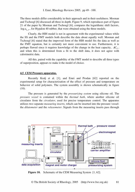
4.5 CEM Pressure apparatus.
Recently Kralj et al. [1], and Emri and Prodan [62] reported on the
experimental setup for characterization of the effect of pressure and temperature on
behavior of solid polymers. The system assembly is shown schematically in figure
(10).
The pressure is generated by the pressurizing system using silicone oil. The
pressure vessel is contained within the thermal bath, where another silicone oil
circulates from the circulator, used for precise temperature control. The apparatus
utilizes two separate measuring inserts, which can be inserted into the pressure vessel:
the dilatometer and the relaxometer. Signals from the measuring inserts pass through
Figure 10. Schematic of the CEM Measuring System [1, 62].
data acquisition
circulator
measuring inserts
thermal bath
pressurizing system
pressure vessel
carrier amplifier
electromagnet
magnet and motor charger

I. Emri, Rheology Reviews 2005, pp 49 - 100.
© The British Society of Rheology, 2005 (http://www.bsr.org.uk) 82
the carrier amplifier prior to being collected in digital format by the data acquisition
system.
The magnet and motor charger supplies current to the electromagnet, which
activates the measurement. The same charger also supplies current to the electric
motor of the relaxometer, shown in figure 10, which pre-loads the spring that then
applies the desired torsional deformation (angular displacement), to the specimen.
Specimens can be simultaneously subjected to pressures of up to 500 MPa with a
precision of 0.1MPa± , and to temperatures ranging from –50°C to +120°C with a
precision of ±0.01°C.
The dilatometer measures bulk properties such as the: bulk creep compliance,
( , , )B t T P ; equilibrium bulk creep compliance, ( , ) ( , , )B T P B t T P= → ∞ ; equilibrium
bulk modulus; ( , ) ( , , ) 1/ ( , )K T P K t T P B T P= → ∞ = ; specific volume
( , ) ( , , )v T P v t T P= → ∞ , and thermal (equilibrium) expansion coefficient,
( , ) ( , , )T P t T Pβ β= → ∞ . The measurements are performed by monitoring the
volume change of the specimen, which results from the imposed changes in pressure
and/or temperature, by measuring the change in length of the specimen, ( , , )L t T P ,
with the aid of a built-in Linear Variable Differential Transformer (LVDT). The
volume estimate can be considered accurate if the change in volume is small (up to a
few percent) and the material is isotropic. Specimens for the dilatometer can be up to
16 mm in diameter and from 40 to 60 mm in length. The absolute volume
measurement error is about 0.1%, while the relative error is 0.05%.
The relaxometer measures the shear relaxation modulus by applying a constant
torsional strain to a cylindrical specimen, in which the induced moment is monitored
over time. The two main parts of the insert are the loading device and the load cell.
The loading device applies a constant torsional strain by twisting the specimen for a
few degrees in less than 0.01 seconds. The deformation of the specimen occurs by first
pre-loading an Archimedes spring with the electric motor. Once twisted, the spring is
kept in its pre-loaded position by a pawl-rack mechanism. Then, the electric magnet,
mounted outside the pressure vessel, pulls the pawl out of the rack, and the energy of
the spring deforms the specimen to a pre-determined angle, which can range from 1°
to 15°. The induced moment is then measured by the load cell, which is attached to the
slider mechanism to compensate for specimen's length changes, resulting from various
temperature and pressure conditions. After the shear relaxation measurement is
complete, the electric motor brings the specimen to its original undeformed state,
while maintaining the pressure vessel fully pressurized. Specimen’s diameter can
range from 2.5 mm to 12 mm while its length from 50 mm to 58 mm. The relaxometer
can measure shear moduli ranging from 0.01MPa to 10.000 MPa , with accuracy
within 5%± of the initial specimen’s modulus value.
The measuring capabilities of the system are summarized in table 4. In the upper
part are listed physical quantities that are measurable “directly”. These are the shear
moment, ( , , )M t T P , and the specimen length, ( , , )L t T P , measured as functions of
time at selected temperatures and pressures. In the second part of table 4 are listed
quantities that may be calculated from “simple definitions”. The third part lists
quantities that need to be extracted from the WLF and/or FMT model.

I. Emri, Rheology Reviews 2005, pp 49 - 100.
© The British Society of Rheology, 2005 (http://www.bsr.org.uk) 83
Physical Properties Symbols
Measured Shear moment. ( ), ( ), ( )M t M T M P or ( , , )M t T P
Specimen length. ( ), ( ), ( )L t L T L P or ( , , )L t T P
Calculated
from
definitions
Shear relaxation modulus. ( ), ( ), ( )G t G T G P or ( , , )G t T P
Specific volume. ( ), ( ), ( )v t v T v P or ( , , )v t T P
Linear thermal expansion
coefficient. ( ), ( )T Pα α or ( , )T Pα
Volumetric thermal
expansion coefficient. ( ), ( ), , ,g e fT Pβ β β β β or , , ( , )g e f T Pβ
Bulk creep compliance. ( ), ( ), ( )B t B T B P or ( , , )B t T P
Bulk modulus. ( ), ( )K T K P or ( , )K T P
Calculated
from models
WLF constants. 1 2, c c
WLF material parameters. 0,
ffα
FMT constants. 1 2 3 4 5 6, , , , , c c c c c c
FMT material parameters. *
0( ), ( ), , , , , f e e
P f P B K k K kα Φ Φ
Table 4: Measuring capabilities of the CEM apparatus.
All together, the system measures five physical quantities: temperature, ( )T t ;
pressure, ( )P t ; torsional deformation (angular displacement) per unit length, 0ϑ ,
applied to the specimen at 0t = ; specimen length ( , , )L t T P ; and the decaying torque,
( , , )M t T P , resulting from the initial torsional deformation, 0ϕ . Using these physical
quantities, measured at constant or varying temperature and pressure, we can obtain
the material properties listed in table 4.
5. SUPERPOSITION IN THE TRANSITION REGION.
There are two features that require comment. The first is the effect of rigid
particulate or fibrillar fillers, and – in crosslinked materials – the effect of the crosslink
density on time-temperature superposition. There is currently no information on the
effect of fillers and of crosslink density on time-pressure superposition. The second is
the effect of temperature and pressure not on the time dependence of the mechanical
behavior but on the response functions themselves. The effect of temperature may be
accounted for by applying vertical shifts. No vertical shifts have been suggested as yet
for time-pressure superposition.

I. Emri, Rheology Reviews 2005, pp 49 - 100.
© The British Society of Rheology, 2005 (http://www.bsr.org.uk) 84
5.1 Fillers and crosslinks.
Polymeric materials may be filled to varying degrees with a rigid filler that
itself shows no appreciable time-temperature-pressure dependence. If the filler itself
shows time dependence, the material is a two-phase material and is not thermo-
rheologically simple. If the volume fraction, ψ , of a rigid filler is not too large, the
filled material generally obeys the WLF equation governing the behavior of the
matrix. The parameters of the equation may change, however, if ψ is large enough to
affect the mobility of the chains of the matrix polymer. They may also change if the
matrix polymer adheres to the filler. In a filled elastomer one distinguishes reinforcing
fillers, the addition of which enhances rupture strength (e.g., certain types of carbon
black,) and non-reinforcing fillers (e.g., salts or glass beads). Stacer and Husband [63]
found that in systems in which the polymer is weakly adsorbed to a non-reinforcing
filler an interface may form that introduces a secondary transition. Application of the
WLF equation is then affected by the existence of this secondary transition. If the
polymer chains are strongly adsorbed to the particles of a reinforcing filler (as is the
case, e.g., with certain types of carbon black) the filler particles can act as (physical)
cross links. Duperray and Leblanc [64] found that in elastomers highly filled with
carbon black ( )E ω′ and ( )E ω′′ did not superpose with the same parameters of the
WLF equation. They also found that in their highly filled systems the distribution of
relaxation times did not conform to equation (1).
Elastomers form a three-dimensional network of covalently (chemically)
cross-linked polymer chains. In chemically crosslinked systems the density of
cross-linking can influence superposability. A high degree of cross linking as is
present in, e.g., the phenolics and melamines, may drastically lower chain mobility,
and therefore the threshold temperature, turning WLF into something resembling an
RP behavior (see section 2.7).
5.2 Vertical shifts.
Successful application of the superposition principles may require certain
adjustments (vertical shifts) to the linear viscoelastic responses such as the moduli,
compliances, viscosities and fluidities, Ferry [31], chapter 11). The vertical shifts take
the form exemplified by:
0 0( ) ( )p
TG t G t
T
ρ
ρ= , ………. (112)
and/or
0 0
( ) ( )p
TJ t J t
T
ρ
ρ= , ………. (113)
where the subscript p refers to the vertically shifted response function, and ρ and
0ρ are the density of the polymer at T and 0T , respectively. The ratio 0 0/T Tρ ρ its
reciprocal are referred to as the vertical shift factors. The density ratio is often omitted

I. Emri, Rheology Reviews 2005, pp 49 - 100.
© The British Society of Rheology, 2005 (http://www.bsr.org.uk) 85
because – particularly when plotting the response function in logarithmic coordinates –
it is deemed negligible.
The blanket application of the vertical shift factors does not appear to be
incontrovertible in all cases. The various components of the response functions
generally require different adjustments. We first consider the stress-response functions
exemplified by the (shear) creep compliance:
[ ] { }( ) ( ) 1 exp( / ) lng f
J t J L t d tτ τ τ φ∞
−∞
= + − +∫ . ………. (114)
Here gJ , the glass compliance, represents the purely elastic, the integral over the
retardation spectrum, ( )L τ represents the viscoelastic, and f tφ represents the purely
viscous contribution. In the latter 1/f fφ η= is the steady-state fluidity, the reciprocal
of the steady-state viscosity. The braces around the last term signify that this term is
absent if the material is arrheodictic (i.e., does not show steady-state flow; see
Tschoegl [2], p. 93).
The vertical shift factor 0 0/T Tρ ρ , being suggested by the flexible chain theory
(Ferry 31, chapter 11), is really not applicable to the glass compliance, gJ . Excluding
gJ from the vertical shift leads to:
0 0
( ) ( )p g g
TJ t J J t J
T
ρ
ρ = + − , ………. (115)
and this equation has indeed found application.
McCrum [65] defined three vertical shift factors, Tb , Tc , and Td , which he
applied to the creep compliance. We follow here McCrum’s notation to indicate the
temperature dependence of the compliances as superscripts. The coefficient Tb is the
ratio of the difference, TeJ and T
gJ , between the equilibrium and the glassy shear
compliance at the temperature, T, to the same difference, 0TeJ and 0T
gJ , at the reference
temperature, 0T . Thus:
0 0
T T
e g
T T T
e g
J Jb
J J
−=
−. ………. (116)
The coefficient Tc is given by:
0
T
g
T T
g
Jc
J= , ………. (117)
and the factor Td by:
0
T
e
T T
e
Jd
J= . ………. (118)

I. Emri, Rheology Reviews 2005, pp 49 - 100.
© The British Society of Rheology, 2005 (http://www.bsr.org.uk) 86
McCrum used these vertical shift factors to obtain ( )TPJ t in a procedure that is too
involved to be reproduced here in detail. The reader is referred to the original
references (McCrum and Morris [65], McCrum et al. [66], and McCrum [67]).
In the strain-response functions exemplified by the (shear) modulus the
viscoelastic and the viscous contributions are not separated from one another. The
(shear) relaxation modulus is given by:
{ }
[ ]
( ) ( ) exp( / ) ln
( ) 1 exp( / ) ln ,
e
g
G t G H t d
G H t d
τ τ τ
τ τ τ
∞
−∞
∞
−∞
= +
= + −
∫
∫
………. (119)
where the viscoelastic and the viscous component are combined into a single
expression, eG being the equilibrium, and gG the glassy modulus, while ( )H τ is the
relaxation spectrum. The braces around eG signify that eG is absent if the material is
rheodictic. On the basis of the second of equations (119) we may argue that the glassy
component, gG , may be separated out from the viscoelastic-viscous component and
that we may hence write:
0 0( ) ( )p g g
TG t G G t G
T
ρ
ρ = + − , ………. (120)
in analogy with the case of ( )J t . We note that [2]:
{ } { }0 01
e eG J = , 1
g eG G = , and 1
f fη φ = , ………. (121)
and their relation to the relaxation, ( )H τ and the retardation, ( )L τ , spectra:
{ } ( ) lng e
G G H dτ τ∞
−∞
− = ∫ , ………. (122)
{ }0( ) ln
e gJ J L dτ τ
∞
−∞
− = ∫ , ………. (123)
and
( ) lnf
H dη τ τ τ∞
−∞
= ∫ . ………. (124)
A different vertical shift procedure was advocated by Rusch [68, 69] who proposed to
use / eT T where eT is the ‘effective’ temperature (see section 6.1) for the vertical shift
factor but admitted that this suggestion lacks theoretical (physical) foundation.
Although no use of vertical shift factors has hitherto been reported in dealing
with time-pressure superposition, the change in density, 0( ) ( )P Pρ ρ might evidently
be considered.
I. Emri, Rheology Reviews 2005, pp 49 - 100.
© The British Society of Rheology, 2005 (http://www.bsr.org.uk) 87
6. SUPERPOSITION IN THE GLASSY REGION
We have discussed the effect of temperature on the mechanical properties of
polymeric materials in the (main) transition region (cf. figure 3), i.e., in the region
between the glassy and the rubbery or the plateau region, in which the response times
arise from segmental motions of the backbone chains. Special considerations apply
outside this region. In the glassy region, i.e., below g
T , or above g
P , segmental
rearrangements of the backbones cannot be detected on the time scale of any
experiment executed in an affordable time frame. The material is, however, not in
thermodynamic equilibrium and generally undergoes structural changes commonly
referred to as physical aging. In the presence of physical aging any possible shift
function becomes a function of time. Because of the absence of equilibrium these
changes are outside the scope of this paper (cf., however, Emri et al. [70]).
Nevertheless, two topics concerning time-temperature superposition in the glassy
region do need to be mentioned here.
6.1. Applicability of the WLF equation in the glassy region.
In the glassy region any attempt to shift isothermal segments into superposition
cannot follow an equation of the WLF type as discussed in section 2.2. All equations
of the WLF type predict that log Ta diverges when 2
g
gT T c= − . Thus T must be larger
than 2
g
gT c+ . Indeed, it is found that values of log Ta , determined experimentally by
shifting, depart from the prediction of the WLF equation and begin to ‘bend over’
below the glass transition temperature. This is shown in figure 11 adapted from
Schwarzl and Zahradnik [32].
Rusch [68] suggested that time-temperature superposition below gT at constant
pressure be effected using a modified WLF equation that makes use of the ‘effective’
temperature of Tool [71]. The reader is referred to Rusch’s original article for details.
In the glassy state polymers are, in principle, always in a non-equilibrium state. The
properties of the material depend on the path along which material has entered the
glassy state. If materials are far below the glass transition then their properties are
time-independent for all practical purposes. However, in the vicinity of the glass
transition materials exhibit significant time-dependent changing of all physical
properties, known as physical aging. Kovacs [72] was among the first who studied
these phenomena. We will refrain from reviewing the phenomena of physical aging
because this subject requires a paper on its own.
6.2 Higher-order transitions.
In virtually all polymers there exist below the glass transition temperature so-
called secondary, tertiary, etc., transitions. These β-, γ-, etc., transitions are distinct
from the α-, or main, transition. While the latter results from the motion of chain
segments, the higher-order transitions arise not from main chain segmental motion but,
typically, from motion of side chains attached to the main chain, or from crankshaft
and kink motions, or other molecular rearrangements (Ferry [31], pp. 450-451). Often

I. Emri, Rheology Reviews 2005, pp 49 - 100.
© The British Society of Rheology, 2005 (http://www.bsr.org.uk) 88
a secondary transition appears to be characterized by a single response time. More
generally it, also, exhibits a distribution of response times just as a main transition
does, although a secondary transition is usually less broad.
It is sometimes claimed that time-temperature superposition of secondary and
higher-order transitions can be effected using the physical equivalent of the Arrhenius
equation (38). This assumes the threshold temperature, LT , for one of these transitions
to be the absolute zero of temperature. The applicability of equation (38) to secondary
transitions is, however, questionable on theoretical grounds. It is unlikely that these
motions should ‘freeze in’, as it were, at 0T = . The molecular motions giving rise to
higher transitions also require free volume in which to move. It is more likely,
therefore, that these transitions should also obey a relation of the form of equation (40)
albeit with a rather low threshold temperature of possibly only a few degrees Kelvin.
Equation (40) with such a low LT would be difficult to distinguish from equation (38).
Be that as it may, however, we may expect that advances in the accuracy of
determining and reporting linear viscoelastic responses will force a more fundamental
look at the presence of secondary transitions in the future. Ferry [31] (page 310), has
carefully investigated time-temperature superposition in the β-transition of poly(n-
butyl methacrylate). Knauss and Zhu [73] have more recently investigated the β-
transition of polycarbonate.
Since superposition does not apply in the presence of more than one
viscoelastic mechanism [cf. equation (1)], the question arises whether thermo-
rheologically simple materials exist at all. Strictly speaking, neither the WLF nor the
FMT equation is valid in cases where the material exhibits higher-order transitions.
Figure 11: The logarithmic shift factor, log Ta , above and below gT .
-20 -10 2010
-2
-4
2
T-T Csº
c1s
c2s
log (T, T ) PSa s
experimental shift
WLF approximation

I. Emri, Rheology Reviews 2005, pp 49 - 100.
© The British Society of Rheology, 2005 (http://www.bsr.org.uk) 89
However, since the α-transition generally overwhelms the behaviour resulting from the
presence of secondary and also higher-order transitions, the influences of the latter
have commonly been neglected. This practice is bolstered by the fact that linearly
viscoelastic responses are generally reported in logarithmic coordinates that normally
mask the relatively small effect of the higher transitions. Also, the presence of
secondary transitions may not unduly affect the location or breadth of the α-transition.
Certainly, when a polymer may be deemed thermo-rheologically simple, time-
temperature superposition affords a welcome means of extending the experimental
time scale.
7. SUPERPOSITION IN THE RUBBERY AND PLATEAU REGIONS
Completely different problems may arise in the rubbery and plateau regions and
in the terminal or flow region. We only briefly refer here to material characteristics
that would influence any superposition scheme in their presence, even though no such
schemes have as yet been proposed and their development may, in fact, be illusory.
Again, contour plots may furnish the only workable data representation in the presence
of some of these characteristics.
7.1 Crystallinity and crosslinking.
If the structure of a polymer chain is sufficiently regular, or if it contains long
enough sequences that have a regular structure, the regions of regular structure will
‘close-pack’, i.e., they will form crystallites, dendrites, or spherulites, structures of
increasing complexity [74-79]. The presence of crystalline structures raises the
modulus in the plateau region, as illustrated in figure 12.
An increase in the degree of crystallinity, ξ, broadens the plateau region and
moves it to shorter times. The dotted line represents the hypothetical case of 100%
crystallinity. As observed by Prodan [42] on polyamide (PA6), this effect of
crystallinity may appear at lower values of ξ and at shorter times, in creep than in
relaxation.
Crystalline regions may interconnect to form superstructures [80]. A
superstructure is a network of crystalline regions interconnected by chains that leave
and enter several of them in sequence. The formation of superstructures is generally
enhanced by orientation brought about by, for instance, drawing or rolling.
Superstructure increases the value of ξ as revealed most clearly by small angle x-ray,
and NMR analysis [81].
A crystalline polymer does not exhibit a well-defined melting point but a
melting region whose extend depends primarily on the degree of crystallinity, and the
molecular mass (weight) distribution of the crystalline regions. Furthermore, the
breadth of the melting regions depends on the rate of heating or cooling applied. In the
construction of contour plots for crystalline polymers the thermal history must
therefore be carefully stated.
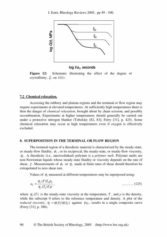
I. Emri, Rheology Reviews 2005, pp 49 - 100.
© The British Society of Rheology, 2005 (http://www.bsr.org.uk) 90
7.2 Chemical relaxation.
Accessing the rubbery and plateau regions and the terminal or flow region may
require experiments at elevated temperatures. At sufficiently high temperatures there is
then the danger of chemical relaxation, brought about by chain scission, and possibly
recombination. Experiments at higher temperatures should generally be carried out
under a protective nitrogen blanket (Tobolsky [82, 83]; Ferry [31], p. 425). Some
chemical relaxation may occur at high temperatures even if oxygen is effectively
excluded.
8. SUPERPOSITION IN THE TERMINAL OR FLOW REGION
The terminal region of a rheodictic material is characterized by the steady-state,
or steady-flow fluidity, fφ , or its reciprocal, the steady-state, or steady-flow viscosity,
fη . A rheodictic (i.e., uncrosslinked) polymer is a polymer melt. Polymer melts are
non-Newtonian liquids whose steady-state fluidity or viscosity depends on the rate of
shear, γ& . Measurements of fφ or fη made at finite rates of shear should therefore be
extrapolated to zero shear rate.
Values of fη measured at different temperatures may be superposed using:
0 0
0
( )
( )
f
T
f
T Ta
T T
η ρ
η ρ= , ………. (125)
where ( )f Tη is the steady-state viscosity at the temperature, T , and ρ is the density,
while the subscript 0 refers to the reference temperature and density. A plot of the
reduced viscosity, 0( ) ( )rη η γ η γ= & & against Taγ& , results in a single composite curve
(Ferry [31], p. 380).
Figure 12: Schematic illustrating the effect of the degree of
crystallinity, ξ , on ( )G t .
log t/aT, seconds
log G
(t),
MP
a
ξ1
ξ2
ξ3
log t/aT, seconds
log G
(t),
MP
a
ξ1
ξ2
ξ3

I. Emri, Rheology Reviews 2005, pp 49 - 100.
© The British Society of Rheology, 2005 (http://www.bsr.org.uk) 91
Superstructures (cf. section 7.1) can persist in the flow region and can interfere
with superposability. Careful measurements by Plazek [8, 84] have shown that shift
factors in the transition and in the terminal zone may be somewhat different. Other
observations of this kind are discussed by Ferry 31, pp. 305ff.
Prodan [42] shifted creep and relaxation data on polyamide (PA6), and
constructed master curves for both, applying the same pair of WLF constants.
However, when the two response curves were interconverted (using the
interconversion algorithm described by Tschoegl and Emri [85, 86]), they differed in
their behaviour in the flow region. He tentatively ascribed this to interaction of the
long-chain components of the molecular mass distribution with the crystalline
superstructure.
9. SUPERPOSITION IN DEFORMATIONS OTHER THAN SHEAR.
In small deformation, time- or frequency-dependent changes in shape (shear)
and changes in size (bulk) are neatly separated. The former are expressed by the shear
relaxation and the shear storage and loss modulus, as well as the shear creep and
shear storage and loss compliance, while the latter are described by the bulk
relaxation and bulk storage and loss modulus, as well as the bulk creep and bulk
storage and loss compliance. In this sense the shear and the bulk properties are
fundamental properties. Response functions that describe simultaneously changes in
shape and in size, such as the tensile relaxation modulus and creep compliance, and
the longitudinal bulk relaxation modulus and longitudinal bulk creep compliance, as
well as the corresponding storage and loss functions, are, in this sense, derived
functions.
The superposition models described in this paper treated superposition in terms
of the shear properties. There is compelling evidence for superposability in the tensile
properties also. Evidence for the same in the bulk properties has been claimed by
McKinney and Belcher [47]. Recent measurements of Deng and Knauss [87] and Sane
and Knauss [88] in shear and in bulk on two different specimens of the same PVAc
(poly(vinyl acetate)) sample appear to support this contention. A definite proof would
require measurements in shear and in bulk that were carried out in accordance with the
Standard Protocol proposed by Tschoegl et al. [89].
10. SUPERPOSITION IN ANISOTROPIC MATERIALS.
Linear isotropic materials require two linear viscoelastic functions for a
complete representation of all their time- or frequency-dependent mechanical
properties. Anisotropic materials require more, Tschoegl [2]. Axisymmetric or
transversely isotropic materials require five, and orthotropic or orthorhombic
materials need nine functions. Many industrially important materials exhibit one or the
other form of anisotropy. Drawn fibers are axisymmetric. Films produced by drawing,
or by rolling, in a single direction are orthotropic. Two of the axisymmetric functions
and three of the orthotropic ones describe bulk properties. The full linear viscoelastic

I. Emri, Rheology Reviews 2005, pp 49 - 100.
© The British Society of Rheology, 2005 (http://www.bsr.org.uk) 92
characterization of anisotropic materials is thus a daunting task and relatively little
information on their time-dependent behaviour is available. Ward [90] includes a
chapter on Anisotropic Mechanical Behaviour with a number of useful references. We
conjecture that the effects of time and/or pressure on the manifold response functions
of anisotropic materials may also be described by the WLF or the FMT models,
provided that the functions are linearly viscoelastic. However, there is no satisfactory
evidence on this issue one way or another.
11. CONCLUDING REMARKS AND RECOMMENDATIONS.
In the following, we summarize the salient points of this review and point out
some areas in which work is currently lacking.
• We attempted to critically review models that deal with the superposition of the
effect of time, temperature, and pressure in thermo- and/or piezo-rheologically
simple polymeric materials. Our primary interest is the effect of pressure.
However, we also reviewed the effect of temperature as necessary background.
Pressure has an analogous, but opposite effect to that of temperature. Thus, the
behavior under high pressure is roughly equivalent phenomenologically to the
behavior at low temperature, and vice versa.
• The FMT model appears to predict most satisfactorily and most simply the
combined effect of pressure and of temperature on single-transition polymers in
thermodynamic equilibrium, i.e., on thermo- and piezo-rheologically simple
materials. The FMT model reduces to the WLF model at the reference (usually the
atmospheric) pressure. The former therefore comprises the latter as a special case.
At the reference temperature the FMT model becomes formally analogous to the
FS model. This model therefore handles time-temperature, time-pressure, and
time-temperature-pressure superposition equally well. Being based on the free
volume concept, the semi-empirical molecular parameters of the FMT model are
the fractional free volume in the reference state, f0, the expansion coefficient of
the fractional free volume, ( )f Pα at the pressure P, and the proportionality
factor, B, of the Doolittle equation. At pressures other than atmospheric, the
parameters of the occupied volume, *Kφ and kφ , are also required. Performing
experiments based on temperature variation alone is not sufficient to calculate
correct values of 0f and fα , since the value for B must be pre-assumed. When
the measurements are executed as function of pressure as well as temperature, the
value of B, 0f and fα as well as *Kφ and kφ , become uniquely determined.
• Time-temperature-pressure superposition is intrinsically unavailable for multi-
phase and multi-transition materials. It may therefore not be strictly applicable to
any polymeric material since secondary transitions are always present. Therefore,
renewed efforts must be made to extend the experimental window through which
materials are viewed, as well as the accuracy with which the measurements are
performed.
• The traditional way of extending the experimental window is the combination of
measurements made as functions of the time and of the frequency. Such
I. Emri, Rheology Reviews 2005, pp 49 - 100.
© The British Society of Rheology, 2005 (http://www.bsr.org.uk) 93
measurements must be converted into one another using an interconversion
algorithm. See, for instance, Baumgaertel and Winter [91] on converting dynamic
data, or Tschoegl and Emri [85, 86] and Emri and Tschoegl [92, 93, 94] on a
rather more general method.
• Combining measurements made in the frequency as well as in the time domain is
often unsatisfactory because of small variations in specimen properties and/or
initial and boundary conditions (such as temperature, pressure, and/or humidity) if
the measurements are not made on the same specimen and under the same
experimental conditions. Tschoegl et al. [89] have proposed a Standard Protocol
to be followed in such measurements. This is particularly important with any of
the time-dependent bulk properties. These are critically dependent on highly
accurate measurements because of their weak dependence on time or frequency.
• To extend the width of the experimental window there is a very definite need for
the development of novel apparatus in which measurements may be performed in
the frequency as well as in the time domain on the same sample and under
identical experimental conditions by simply throwing a switch, as it were. The
development of such an apparatus is within the capability of present day
technology and should be undertaken forthwith.
• The effect of temperature and/or pressure on the mechanical properties of
polymeric materials in the general case requires the construction of contour plots.
Such plots will, however, be truly useful only if the data can span a sufficiently
wide swath of the time and/or the frequency scale. The computer program
employed for the construction of a contour plot should allow the user to recover at
will the effect of temperature or pressure at a selected time or frequency, or the
effect of time or frequency at a selected temperature or pressure. Programs of this
kind are now available.
• We recommend the compilation of the parameters of the FMT equation on a
number of the more important polymeric materials. Since this work will entail a
determination of the pre-exponential factor, B, it will at the same time allow re-
examination of the parameters of the WLF equation for the same materials. This
work has now been initiated by Kralj et al. [1] and Emri and Prodan [62].
• The problem whether the superposition of the bulk properties follows the same
rules (the WLF and/or the FMT equation) as do the shear properties should be
resolved unambiguously. It is now almost universally accepted that the
superposition of tensile properties follows the same rules as does that of the shear
properties. If bulk behavior follows different rules, the tensile behaviour must be
re-examined.
• Another unresolved problem is that of the time-pressure superposition of the
mechanical properties of polymers in the glassy region, i.e., above gP [42].
• Finally, the emerging technology of multi-component injection molding requires
knowledge of the effects of temperature and pressure variation on each
component upon cooling. This affects the mechanical, optical, electrical, and
possibly other physical properties of the assembly.
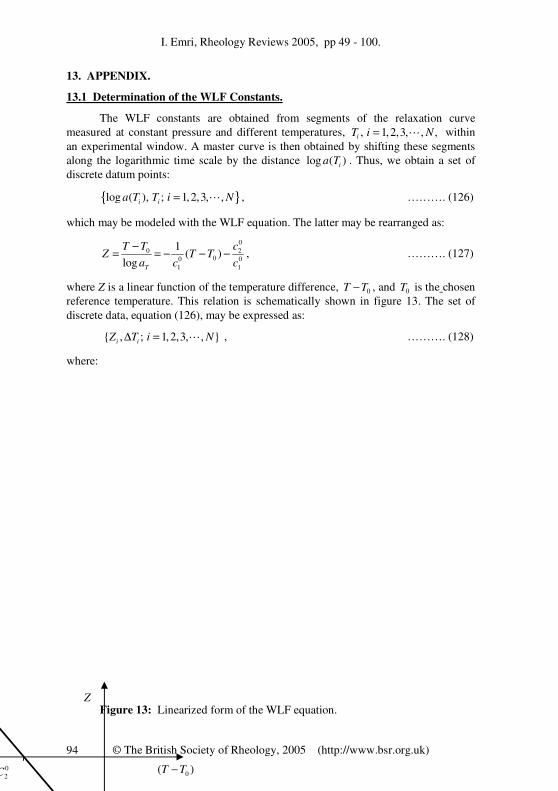
I. Emri, Rheology Reviews 2005, pp 49 - 100.
© The British Society of Rheology, 2005 (http://www.bsr.org.uk) 94
13. APPENDIX.
13.1 Determination of the WLF Constants.
The WLF constants are obtained from segments of the relaxation curve
measured at constant pressure and different temperatures, , 1,2,3, , ,iT i N= L within
an experimental window. A master curve is then obtained by shifting these segments
along the logarithmic time scale by the distance log ( )i
a T . Thus, we obtain a set of
discrete datum points:
{ }log ( ), ; 1,2,3, ,i i
a T T i N= L , ………. (126)
which may be modeled with the WLF equation. The latter may be rearranged as:
0
0 200 0
1 1
1( )
logT
T T cZ T T
a c c
−= = − − − , ………. (127)
where Z is a linear function of the temperature difference, 0T T− , and 0T is the chosen
reference temperature. This relation is schematically shown in figure 13. The set of
discrete data, equation (126), may be expressed as:
{ , ; 1,2,3, , }i i
Z T i N∆ = L , ………. (128)
where:
Figure 13: Linearized form of the WLF equation.
0( )T T−
Z
0
2C−

I. Emri, Rheology Reviews 2005, pp 49 - 100.
© The British Society of Rheology, 2005 (http://www.bsr.org.uk) 95
0
log ( ) log ( )
i i
i
i i
T T TZ
a T a T
− ∆= = . ………. (129)
Each discrete value iZ may be modeled with the WLF equation, equation (11), as:
0
2
0 0
1 1
1( )
i i i i i
cZ Z T T
c cδ δ= ∆ + = − ∆ − + , ………. (130)
where iδ is the approximation error of modeling the iZ with the WLF equation.
Introducing the notation 011/a c= − and 0 0
2 1/b c c= − we can re-write equation (130)
as:
( )i i i i i
Z Z T a T bδ δ= ∆ + = ∆ + + , ………. (131)
from which we find the approximation error for each iZ as:
( )i i iZ a T bδ ∆= − + . ………. (132)
Furthermore, we may write:
2 2
1 1
[ ( )]N N
i i i
i i
Z a T bΛ δ ∆= =
= = − +∑ ∑ . ………. (133)
Minimizing the sum of the squares with respect to a and b we obtain:
1
2 [ ( )] 0N
i i i
i
Z a T b Ta =
∂Λ= − − ∆ + ∆ =
∂∑ . ………. (134)
After some rearrangement we get:
2
1 1 1
1 1
N N N
i i i i
i i i
N N
i i
i i
aT T Z T
T N Zb
∆ ∆ ∆
∆
= = =
= =
=
∑ ∑ ∑
∑ ∑. ………. (135)
The solution of this matrix equation is given by:
aDa
D= , and bD
bD
= , ………. (136)
where:
2
1 1
1
N N
i i
i i
N
i
i
T T
D
T N
= =
=
∆ ∆
=
∆
∑ ∑
∑, ………. (137)

I. Emri, Rheology Reviews 2005, pp 49 - 100.
© The British Society of Rheology, 2005 (http://www.bsr.org.uk) 96
1 1
1
N N
i i i
i i
a N
i
i
Z T T
D
Z N
∆ ∆= =
=
=
∑ ∑
∑, ………. (138)
and
2
1 1
1 1
ZN N
i i i
i i
b N N
i i
i i
T T
D
T Z
∆ ∆
∆
= =
= =
=
∑ ∑
∑ ∑. ………. (139)
Solving the above determinants we find the constants 0
1c and 0
2c to be given as:
2
2
1 101
1 1 1
1
N N
i i
i i
N N N
i i i
i i i
T N T
ca
N Z T Z T
∆ ∆
∆ ∆
= =
= = =
−
= − =
−
∑ ∑
∑ ∑ ∑, ………. (140)
and
2
1 1 1 102
1 1 1
N N N N
i i i i i
i i i i
N N N
i i i
i i i
T Z Z T Tb
ca
N Z T Z T
∆ ∆ ∆
∆ ∆
= = = =
= = =
−
= =
−
∑ ∑ ∑ ∑
∑ ∑ ∑. ………. (141)
ACKNOWLEDGEMENTS
This work was supported by the Ministry of Science, Education and Sports of the
Republic of Slovenia.
The author gratefully acknowledges the cooperation of Aleš Kralj and Ted
Prodan of the Center of Experimental Mechanics at the University of Ljubljana in
assembling and excerpting references. Special thanks are due to Ted Prodan for
preparing several of the figures.
REFERENCES
1. Kralj, A, Prodan, T and Emri, I, J. Rheol., 45 (2001) 929-943.
2. Tschoegl, N W, “The Phenomenological Theory of Linear Viscoelastic
Behavior”, Springer-Verlag, Berlin, (1989).
3. Gross, B, “Mathematical Structure of the Theories of Viscoelasticity”,
Hermann et Cie., Paris, (1968).

I. Emri, Rheology Reviews 2005, pp 49 - 100.
© The British Society of Rheology, 2005 (http://www.bsr.org.uk) 97
4. Gross, B, J. Appl. Phys., 40 (1969) 3397.
5. Fillers, R W and Tschoegl, N W, Trans. Soc. Rheol., 21 (1977) 51-100.
6. Moonan, W K and Tschoegl, N W, J. Polym. Sci., Polym. Phys. Ed., 23 (1985)
623-651.
7. Rusch, K C, J. Macromol. Sci.-Phys., B2 (1968) 421-447.
8. Plazek, D J, J. Polym. Sci., A2(6) (1968) 621-638
9. Fesko, D G and Tschoegl, N W, J. Polym. Sci., Part C, Symposia, 35 (1971)
51-69.
10. Fesko, D G and Tschoegl, N W, Internat. J. Polym. Mater., 3 (1974) 51-79.
11. Kaplan, D and Tschoegl, N W, Polym. Engrg. Sci., 14 (1974) 43-49.
12. Cohen, R E and Tschoegl, N W, Trans. Soc. Rheol., 20 (1976) 153-169
13. Brinson, L C and Knauss,W G, J. Mech. Phys. Solids, 39 (1991) 859-880.
14. Brinson, L C and Knauss, W G, J. Appl. Mech., 59 (1992) 730-737.
15. Caruthers, J M and Cohen, R E, Rheol. Acta, 19 (1980) 606-613.
16. Shen, M C and Eisenberg, A, Prog. Solid State Chem., 3 (1966) 407-481.
17. Moonan, W K and Tschoegl, N W, Macromolecules, 16 (1983) 55-59.
18. Tschoegl, N W, “Fundamentals of Equilibrium and Steady-State
thermodynamics”, Elsevier, Amsterdam, (2000).
19. Gibbs, J A and DiMarzio, E A, J. Chem. Phys., 28 (1958) 373-383.
20. DiMarzio, E A and Gibbs, J H, J. Chem. Phys., 28 (1958) 807-813.
21. DiMarzio, E A. and Gibbs, J H, J. Polym. Sci., 40 (1959) 121-131.
22. DiMarzio, E A and Gibbs, J H, J. Polym. Sci. A1 (1963) 1417-1428.
23. DiMarzio, E A and Gibbs, J H, J. Res. Nat. Bur. Stand, A68 (1964) 611-617.
24. DiMarzio, E A, Gibbs, J H, Fleming III, P D and Sanchez, I C,
Macromolecules, 9 (1976) 763-771.
25. Gibbs, J A, “Modern Aspects of the Vitreous State”, Butterworths, London,
(1960).
26. Paterson, M S, J. Appl. Phys., 35 (1964) 176-179.
27. Bianchi, U, J. Phys. Chem., 69 (1965) 1497-1504.
28. Matheson, A J, J. Chem. Phys., 44 (1966) 695-699.
29. Doolittle, A K and Doolittle, D B, J. Appl. Phys., 28 (1957) 901-905.
30. Williams, M L, Landel, R F and Ferry, J D, J. Amer. Chem. Soc., 77 (1955)
3701-3707.

I. Emri, Rheology Reviews 2005, pp 49 - 100.
© The British Society of Rheology, 2005 (http://www.bsr.org.uk) 98
31. Ferry, J D, “Viscoelastic Properties of Polymers”, 3rd Ed., Wiley and Sons,
New York, (1980).
32. Schwarzl, F R and Zahradnik, F, Rheol. Acta, 19 (1980) 137-152.
33. Bueche, F, J. Chem. Phys., 36 (1962) 2940-2946.
34. Bestul, A B and Chang, S S, J. Chem. Phys., 40 (1964) 3731-3733.
35. Chang, S S, Bestul, A B and Horman, J A, in Proceedings of the VII
International Congress on Glass, Brussels, (1965).
36. Goldstein, M, J. Chem. Phys., 39 (1963) 3369-3374.
37. Adam, G and Gibbs, J H, J. Chem. Phys., 43 (1965) 139-146.
38. Kauzmann, W, Rev. Mod. Phys., 14 (1942) 12–44.
39. Eisenberg, A and Saito, S, J. Chem. Phys., 45 (1966) 1673-1678.
40. Hutchinson, J M and Kovacs, A J, J. Polym. Sci.: Polym. Phys. Ed., 14 (1976)
1575-1590.
41. Moonan, W K and Tschoegl, N W, Internat. Polym. Mater., 10 (1984) 199-211.
42. Prodan, T, ‘The effect of pressure and temperature on the shear relaxation
behaviour of time-dependent materials’, Ph.D. Thesis, Department of
Mechanical Engineering, University of Ljubljana, Slovenia, (2002).
43. Bridgman, P W, “The Physics of High Pressure”, G. Bell and Sons, London,
(1949).
44. Gee, G, Polymer, 7 (1966) 177-191.
45. Havliček, I, Ilavsky, M and Hrouz, J, J. Macromol. Sci. Phys, B21 (1982) 425-
441.
46. Ferry, J D and Stratton, R A, Kolloid-Z., 171 (1960) 107-111.
47. McKinney, J E and Belcher, H V, J. Res. Nat. Bur. Stand., 67A (1963) 43-53.
48. Tribone, J J, O’Reilly, J M and Greener, J, J. Polym. Sci.: Part B: Polym.
Phys., 27 (1989) 837-857.
49. Freeman, B D, Bokobza, L and Monnerie, L, Polymer, 31 (1990) 1045-1050.
50. O’Reilly, J M, J. Polym. Sci., 57 (1962) 429-444.
51. O’Reilly, J M, Tribone, J J and Greener, J, Polym. Sci., Polym. Phys. Ed., 26
(1988) 501-513.
52. Ramos, A R, Kovacs, A J, O’Reilly, J M, Tribone, J J and Greener, J, J. Polym.
Sci., Polym. Phys. Ed., 26 (1988) 501-513.
53. Tait, P, “Physics and Chemistry of the Voyage of H.M. Ship Challenger”, Vol.
II, Cambridge University Press, Cambridge, (1900).
54. Boldizar, A, Kubát, J and Rigdahl, M, J. Appl. Polym. Sci., 39 (1990) 63-71.

I. Emri, Rheology Reviews 2005, pp 49 - 100.
© The British Society of Rheology, 2005 (http://www.bsr.org.uk) 99
55. Simha, R and Somcynsky, T, Macromolecules, 2 (1969) 342-350.
56. Simha, R and Wilson, P S, Macromolecules, 6 (1973) 902-913.
57. Somcynsky, T and Simha, R, J. Appl. Phys., 42 (1971) 4545-4548.
58. Curro, J G, Lagasse, R R and Simha, R, J. Appl. Phys., 52 (1981) 5892.
59. Utracki, L A, Polym. Engrg. Sci., 23 (1983) 446-451.
60. Utracki, L A, Polym. Prep., Amer. Chem. Soc., 24 (1983) 113.
61. Murnaghan, F D, “Finite Deformation of Elastic Solids”, Wiley, New York,
(1951).
62. Emri, I, Prodan, T, Submitted to Experimental Mechanics, (2004)
63. Stacer, R G and Husband, D M, Rheol. Acta, 29 (1990) 152-162.
64. Duperray, B and Leblanc, J L, Kautschuck + Gummi · Kunststoffe, 35 (1982)
298-307.
65. McCrum, N G, Polymer, 25 (1984) 309-317.
66. McCrum, N G and Morris, E L, Proc. Roy. Soc., A281 (1964) 258-273.
67. McCrum, N G, Read, B E and Williams, G, “Anelastic and Dielectric Effects in
Polymeric Solids”, Wiley and Sons, New York, (1967).
68. Rusch, K C, J. Macromol. Sci.-Phys., B2 (1968) 179-204.
69. Rusch, K C, J. Macromol. Sci.-Phys., B2 (1968) 421-447.
70. Emri, I, Knauss, W G and Tschoegl, N W, ‘Non-equilibrium time-dependent
behaviour of polymeric materials’, (2005), in preparation.
71. Tool, A Q, J. Amer. Ceram. Soc., 29 (1946) 240-253.
72. Kovacs, A J, Adv. Polym. Sci., 3 (1964) 394-507.
73. Knauss, W G and Zhu, W D, Mech. Time-Dependent Mater., (2002), to appear.
74. Wunderlich, B, “Macromolecular Physics, Volume I, Crystal Structure,
Morphology, and Defects”, Academic Press, New York, (1973).
75. Aharoni, S M, “n-Nylons: Their Synthesis, Structure and Properties”, J. Wiley
& Sons, Inc. New York, (1997), and references therein.
76. Eder, G, Janeschitz-Kriegl, H and Liedauer, S, Progr. Polym. Sci. 15(1990),
629-714.
77. Eder, G and Janeschitz-Kriegl, H, ”Structure Development During Processing:
Crystallization”, In H.Meijer (ed.), Materials Science and Technology, Volume
18, Verlag Chemie, (1997).
78. Hearle, J W S, “Fiber formation and the science of complexity; In: Salem,
D.R., Structure Formation in Polymer Fibers”, Carl Hanser Verlag, (2001).

I. Emri, Rheology Reviews 2005, pp 49 - 100.
© The British Society of Rheology, 2005 (http://www.bsr.org.uk) 100
79. Swartjes, F H M, “Flow induced crystallization in elongation flow”, Ph.D.
thesis, Eindhoven Univeristy of Technology, (2001), downloadable from:
www.mate.tue.nl.
80. Emri, I, and von Bernstrorff, B S, Submitted to J. Appl. Mech., (2004).
81. Cevc, P, Arčon, D, Blinc, R, and Emri, I, “Electron Paramagnetic Resonance of
Stressed Fiber Nylon 6: Annealing Effects”, In preparation, (2005).
82. Tobolsky, A V, “Properties and Structure of Polymers”, Wiley and Sons, New
York, (1960).
83. McLaughlin, J R and Tobolsky, A, J.Colloid Sci, 7 (1952) 555-568.
84. Plazek, D J, J. Phys. Chem., 69 (1965) 3480-3487.
85. Tschoegl, N W and Emri, I, Internat. J. Polym. Mater., 18 (1992) 117-127.
86. Tschoegl, N W and Emri, I, Rheol. Acta, 32 (1993) 322-327.
87. Deng, T H and Knauss, W G, Mech. Time-Dependent. Mater., 1 (1997) 33-49.
88. Sane, S and Knauss, W G, Mech.Time-Dependent Mater., 5 (2001) 293-324.
89. Tschoegl, N W, Knauss, W G and Emri, I, Mech. Time-Dependent. Mater., 6
(2002) 3-51.
90. Ward, I M, “Mechanical Properties of Solid Polymers”, Wiley-Interscience,
London, (1971).
91. Baumgaertel, M and Winter, H H, Rheol. Acta, 28 (1989) 511-519.
92. Emri, I and Tschoegl, N W, Rheol. Acta, 32 (1993) 311-321.
93. Emri, I and Tschoegl, N W, Rheol. Acta, 33 (1994) 60-70.
94. Emri, I and Tschoegl, N W, Internat. J. Polym. Mater., 40 (1998) 55-79.