rg000166 1. - pik-potsdam.de
TRANSCRIPT

ON THE DRIVING PROCESSES OF THE ATLANTIC
MERIDIONAL OVERTURNING CIRCULATION
T. Kuhlbrodt,1 A. Griesel,2 M. Montoya,3 A. Levermann,1 M. Hofmann,1 and S. Rahmstorf1
Received 3 December 2004; revised 10 August 2006; accepted 26 October 2006; published 24 April 2007.
[1] Because of its relevance for the global climate theAtlantic meridional overturning circulation (AMOC) hasbeen a major research focus for many years. Yet thequestion of which physical mechanisms ultimately drive theAMOC, in the sense of providing its energy supply, remainsa matter of controversy. Here we review both observationaldata and model results concerning the two main candidates:vertical mixing processes in the ocean’s interior and wind-induced Ekman upwelling in the Southern Ocean. Indistinction to the energy source we also discuss the role
of surface heat and freshwater fluxes, which influence thevolume transport of the meridional overturning circulationand shape its spatial circulation pattern without actuallysupplying energy to the overturning itself in steady state.We conclude that both wind-driven upwelling and verticalmixing are likely contributing to driving the observedcirculation. To quantify their respective contributions, futureresearch needs to address some open questions, which weoutline.
Citation: Kuhlbrodt, T., A. Griesel, M. Montoya, A. Levermann, M. Hofmann, and S. Rahmstorf (2007), On the driving processes of
the Atlantic meridional overturning circulation, Rev. Geophys., 45, RG2001, doi:10.1029/2004RG000166.
1. INTRODUCTION
[2] The deep Atlantic meridional overturning circulation
(AMOC) consists of four main branches: upwelling pro-
cesses that transport volume from depth to near the ocean
surface, surface currents that transport relatively light water
toward high latitudes, deepwater formation regions where
waters become denser and sink, and deep currents closing
the loop. These four branches span the entire Atlantic on
both hemispheres, forming a circulation system that consists
of two overturning cells, a deep one with North Atlantic
Deep Water (NADW) and an abyssal one with Antarctic
Bottom Water (AABW). A highly simplified, illustrative
sketch of this circulation is given in Figure 1. The AMOC
exerts a strong control on the stratification and distribution
of water masses, the amount of heat that is transported by
the ocean, and the cycling and storage of chemical species
such as carbon dioxide in the deep sea. Thus the AMOC is a
key player in the Earth’s climate. In the North Atlantic its
maximum northward heat transport is about 1 PW (1015 W)
[Hall and Bryden, 1982; Ganachaud and Wunsch, 2000;
Trenberth and Caron, 2001], contributing to the mild
climate predominant in northwestern Europe. A reduction
in AMOC is likely to have strong implications for the
El Nino–Southern Oscillation phenomenon [Timmermann
et al., 2005], the position of the Intertropical Convergence
Zone [Vellinga and Wood, 2002], the marine ecosystem in
the Atlantic [Schmittner, 2005], and the sea level in the
North Atlantic [Levermann et al., 2005]. Evidence from the
geological past [Bond et al., 1992; McManus et al., 2004]
suggests that reorganizations of the AMOC were involved
in climatic temperature changes of several degrees in a few
decades (see also the reviews by Clark et al. [2002] and
Rahmstorf [2002]). In the future, there is a risk that
substantial changes in ocean circulation could occur as a
result of global warming [Manabe and Stouffer, 1994;
Rahmstorf and Ganopolski, 1999; Wood et al., 1999;
Schaeffer et al., 2002; Zickfeld et al., 2007].
[3] Ultimately, the influence of Sun and Moon is respon-
sible for oceanic and atmospheric circulations on Earth. The
surface fluxes of heat, fresh water, and momentum as well
as gravity and tides set the ocean waters in motion, either
directly or via intermediate processes such as waves. The
main aim of this paper is to discuss the physical mecha-
nisms that drive the AMOC in the sense that they provide an
energy input into the ocean that is capable of sustaining a
steady state deep overturning circulation.
[4] Presently, two distinct mechanisms for driving the
meridional overturning circulation (MOC) are discussed.
The first one is the traditional thermohaline driving mech-
anism proposed by Sandstrom [1916] and Jeffreys [1925].
In this view the driver is mixing that transports heat from
the surface to the deepwater masses, downward across
ClickHere
for
FullArticle
1Potsdam Institute for Climate Impact Research, Potsdam, Germany.2Scripps Institution of Oceanography, La Jolla, California, USA.3Departamento Astrofisica y Ciencias de la Atmosfera, Facultad de
Ciencias Fısicas, Universidad Complutense de Madrid, Madrid, Spain.
Copyright 2007 by the American Geophysical Union.
8755-1209/07/2004RG000166$15.00
Reviews of Geophysics, 45, RG2001 / 2004
1 of 32
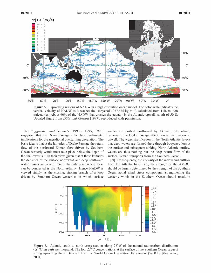
Paper number 2004RG000166
RG2001

surfaces of equal density (diapycnal mixing). Munk and
Wunsch [1998] described this mechanism in detail. The
action of winds and tides generates internal waves in the
oceans. These waves dissipate into small-scale motion that
causes turbulent mixing. This mixing of heat lightens water
masses in the deep ocean and causes them to rise in low
latitudes. Resulting surface and intermediate waters are then
advected poleward into the North Atlantic where they are
transformed into dense waters by atmospheric cooling and
salt rejection during sea ice growth. These waters sink to
depth and spread, setting up the deepwater mass of the
ocean. Thereby a meridional density gradient between high
and low latitudes is established. A sketch of the involved
processes and their locations is given in Figure 2.
[5] The second candidate is wind-driven upwelling, as
put forward by Toggweiler and Samuels [1993b, 1995,
1998]. On the basis of observational radiocarbon constraints
they concluded that the actual amount of upwelling of
abyssal water caused by diapycnal mixing is insufficient
to sustain an estimated overturning of about 15 Sv (1 Sv = 1
Sverdrup = 106 m3 s�1) in the Atlantic Ocean. As an
alternative they suggested that most of the oceanic upwell-
ing is wind-driven and occurs in the Southern Ocean. The
strong westerly circumpolar winds induce a vigorous north-
ward transport of waters, called Ekman transport, near the
ocean surface. Since there is a horizontal divergence of the
Ekman transport, an upwelling from depth is induced that is
associated with the so-called Drake Passage effect (see
Figure 2). In this view it is the strength of Southern Ocean
winds rather than the oceanic diapycnal mixing that governs
the strength of the AMOC. Note that in this theory the
winds induce large-scale motion of the water masses in
the Southern Ocean, which enter the Atlantic and flow to
the northern deepwater formation sites. Wind-driven mix-
ing, i.e., small-scale turbulent motion that is induced by
surface wind stress, is part of the mixing processes and is
not considered as a direct wind-driven upwelling.
[6] Determining which of these two processes is the main
driving mechanism of the MOC is of great interest, even
beyond the mere aim of physical understanding. The two
could imply different sensitivities to variations in external
forcing [Schmittner and Weaver, 2001; Prange et al., 2003]
and thus a different evolution of the MOC under continued
global climate change. In the present paper we review work
on theory, modeling, and observations that argue for either
or both of the possible driving mechanisms.
[7] We wish to emphasize that the driving processes do
not fully determine the AMOC’s spatial extent and strength.
The amount of water that actually sinks in the North
Atlantic is controlled by a variety of processes including
the horizontal gyre circulation, atmospheric cooling, pre-
cipitation, evaporation, and ice melting. These processes
Figure 1. Strongly simplified sketch of the global overturning circulation system. In the Atlantic, warmand saline waters flow northward all the way from the Southern Ocean into the Labrador and NordicSeas. By contrast, there is no deepwater formation in the North Pacific, and its surface waters are fresher.Deep waters formed in the Southern Ocean become denser and thus spread in deeper levels than thosefrom the North Atlantic. Note the small, localized deepwater formation areas in comparison with thewidespread zones of mixing-driven upwelling. Wind-driven upwelling occurs along the AntarcticCircumpolar Current (ACC). After Rahmstorf [2002].
RG2001 Kuhlbrodt et al.: DRIVERS OF THE AMOC
2 of 32
RG2001

can change the AMOC’s spatial pattern drastically, and they
can temporarily reduce or increase the amount of deep water
formed, with a strong impact on climate. However, our
focus here is on the AMOC as a large-scale coherent
circulation system and on longer timescales, that is, on
which mechanism provides the ocean with the energy
necessary to sustain a steady state deep overturning circu-
lation.
[8] The terms ‘‘meridional overturning circulation’’ and
‘‘thermohaline circulation’’ (THC) have sometimes been
used almost like synonyms, but they have very different
meanings. ‘‘MOC’’ is merely a descriptive, geographic
term: It is simply a circulation in the meridional-vertical
plane, as depicted by an overturning stream function as in
Figure 3. The term ‘‘MOC’’ thus does not refer to any
particular driving mechanism.
[9] The term ‘‘THC,’’ by contrast, is a definition of flow
by driving mechanism. There are three qualitatively differ-
ent physical mechanisms to drive oceanic flows: (1) direct
momentum transfer by surface winds, (2) acceleration of
water by tidal forces, and (3) thermohaline forcing. This
classification has been found in oceanography textbooks
since the early 20th century [e.g., Defant, 1929; Neumann
and Pierson, 1966]. A simple, archetypal example of the
latter would be the regional thermohaline (or, in this case,
thermal) circulation caused by ‘‘hot spots’’ of geothermal
heating at the ocean bottom near mid-ocean ridges [Joyce
and Speer, 1987; Thompson and Johnson, 1996]. Another
example is the flow driven by strong surface cooling of a
previously warmer body of water, as occurs, for example,
when a polynya opens up in sea ice [Buffoni et al., 2002]. In
these examples, thermohaline fluxes at the ocean boundary
(surface or bottom) cause density changes that drive a flow
by setting up pressure gradients.
[10] A complication arises when considering the large-
scale thermohaline circulation in steady state, as this steady
Figure 2. Idealized meridional section representing a zonally averaged picture of the Atlantic Ocean.Straight arrows sketch the MOC. The color shading depicts a zonally averaged density profile derivedfrom observational data [Levitus, 1982]. The thermocline, the region where the temperature gradient islarge, separates the light and warm upper waters from the denser and cooler deep waters. The two mainupwelling mechanisms, wind-driven and mixing-driven, are displayed. Wind-driven upwelling is aconsequence of a northward flow of the surface waters in the Southern Ocean, the Ekman transport, thatis driven by strong westerly winds (see section 4). Since the Ekman transport is divergent, waters upwellfrom depth. Mixing along the density gradient, called diapycnal mixing, causes mixing-driven upwelling;this is partly due to internal waves triggered at the ocean’s boundaries (see section 3). Deepwaterformation (DWF) occurs in the high northern and southern latitudes, creating North Atlantic Deep Water(NADW) and Antarctic Bottom Water (AABW), respectively. The locations of DWF are tightly linkedwith the distribution of surface fluxes of heat and fresh water; since these influence the buoyancy of thewater, they are subsumed as buoyancy fluxes. The freshly formed NADW has to flow over the shallowsill between Greenland, Iceland, and Scotland. Close to the zone of wind-driven upwelling in theSouthern Ocean is the Deacon cell recirculation, visible in the zonally integrated meridional velocity inocean models. Its relevance is discussed in section 4. Note that in the real ocean the ratio of themeridional extent to the typical depth is about 5000 to 1.
RG2001 Kuhlbrodt et al.: DRIVERS OF THE AMOC
3 of 32
RG2001

state cannot be maintained by surface buoyancy fluxes
alone. As discussed in detail in section 2, a mechanical
energy input is required to sustain the turbulence necessary
to mix down heat in order to maintain the pressure gradients
in addition to the surface fluxes. To account for this fact, the
large-scale thermohaline circulation has been defined as
‘‘currents driven by fluxes of heat and fresh water across
the sea surface and subsequent interior mixing of heat and
salt’’ [Rahmstorf, 2002, p. 208, 2003]. The same fact is
addressed by the definition of Huang [2004, p. 497]: [The
THC is] ‘‘an overturning flow in the ocean driven by
mechanical stirring/mixing, which transports mass, heat,
fresh water, and other properties. In addition, the surface
heat and freshwater fluxes are necessary for setting up the
flow.’’ However, mechanical stirring is only necessary for
sustaining a steady state large-scale MOC not for the
examples of transient or regional thermohaline flows men-
tioned above. Being aware that the word ‘‘driver’’ is used
with different meanings in the literature, we use it for the
remainder of this paper with the meaning ‘‘the physical
process that provides the necessary energy input to sustain a
steady state deep MOC.’’
[11] Since we discuss both a mechanism to drive the
large-scale MOC directly by winds (section 4) and the
traditional driving mechanism including turbulent mixing
and thermohaline forcing (section 3) in this paper, we will
generally use the driver-neutral terms ‘‘MOC’’ or
‘‘AMOC.’’ We restrict our discussion to the deep MOC,
excluding the shallow Ekman cells of the MOC that are
usually confined to the upper few hundred meters.
[12] The paper is organized as follows. Section 2 deals
with ‘‘Sandstrom’s theorem.’’ On the basis of experiments
and theory it implies that the steady state MOC cannot be
driven by surface buoyancy fluxes alone. We present the
critical discussion that has followed the early statement of
this theorem. A focus is put on the energy budget of the
general circulation. Subsequently, the two possible driving
mechanisms are presented. Diapycnal mixing as a driver is
discussed in section 3, centered around the budget of
turbulent diapycnal mixing energy and its sources, which
are basically winds and tides. In addition, we treat the
fundamental difficulties of representing turbulent mixing
in ocean general circulation models. Surface wind forcing as
a driver is addressed in section 4. This includes tracer
evidence for wind-driven upwelling in the Southern Ocean
and a specific dynamical constraint favoring this upwelling.
Section 4 ends with a revisit to the budget of turbulent
diapycnal mixing energy. We find that likely both mixing
and wind-driven upwelling drive the AMOC. Next, in
section 5 we study the role of the surface buoyancy fluxes
in setting the strength and the shape of the AMOC; today’s
AMOC is characterized by deepwater formation in the
northern North Atlantic and the Southern Ocean. A question
of strong interest is the stability of the AMOC, to which we
devote section 6. Specific issues are the AMOC’s instabil-
ities in past climates and various sources of bistability, like
freshwater fluxes or the different driving mechanisms. A
reason for concern in the near future are transient changes of
the AMOC along with their consequences. In section 7 we
Figure 3. Stream function of the zonally integrated meridional overturning circulation in the Atlan-tic Ocean, as simulated by a coupled ocean-atmosphere model (for a full description of the model seeMontoya et al. [2005]). Contour interval is a fixed volume flux of 3 Sv = 3 � 106 m3 s�1. Solid (dashed)lines indicate a clockwise (a counterclockwise) circulation. While the maximum overturning of the modelNADW (at about 40�N and 1000 m depth) is 15.5 Sv, the outflow at 30�S is only 9.8 Sv. The modelAABW enters the Atlantic with a volume flux of about 3 Sv.
RG2001 Kuhlbrodt et al.: DRIVERS OF THE AMOC
4 of 32
RG2001

summarize the central results and outline the main open
questions.
2. ENERGY BUDGET AND SANDSTROM’STHEOREM
[13] As we will see in sections 3 and 4, the question of
which mechanisms drive the AMOC is intimately linked to
where and how the upwelling of deep water takes place. The
ocean’s mechanical energy is continuously dissipated
through friction. To maintain a steady state circulation, an
energy source is required to overcome friction. Identifying
such a process, its role in the energy budget of the ocean,
and the energy pathways has been the subject of substantial
research in the past decade [e.g., Munk and Wunsch, 1998;
Toggweiler and Samuels, 1998; Huang, 1999; Gade and
Gustafsson, 2004; Huang, 2004; Wunsch and Ferrari,
2004; Gnanadesikan et al., 2005]. Our intention herein is
to review the current understanding.
2.1. Sandstrom’s Theorem
[14] The starting point of discussions on energetics of the
ocean and the drivers of the ocean’s overturning circulation
is often what is commonly known as Sandstrom’s theorem
[e.g., Defant, 1961; Dutton, 1986; Houghton, 1986; Colin
de Verdiere, 1993; Munk and Wunsch, 1998; Huang, 1999;
Gade and Gustafsson, 2004; Huang, 2004; Wunsch and
Ferrari, 2004; Gnanadesikan et al., 2005; Hughes and
Griffiths, 2006]. Sandstrom [1908] performed a series of
tank experiments in which he analyzed under which con-
ditions buoyancy forcing alone, applied at different depths,
could lead to a deep overturning circulation in a water tank.
A heating and a cooling source were placed at opposite
extremes in the tank. In one of the experiments the heating
source was situated above the cooling source; in another
one it was below. Sandstrom [1908] concluded that a
thermally driven, closed, steady circulation in the ocean
can only be established if the heating source is situated at a
lower level than the cooling source.
[15] Sandstrom’s theorem was later put on a more theo-
retical foundation by Sandstrom [1916] and Bjerknes
[1916]. Neglecting the Earth’s rotation, the forces acting
upon a fluid parcel are pressure gradient forces, gravity, and
friction. The circulation equation along a closed streamline
S thus gives [Defant, 1961]:
dC
dt¼ d
dt
IS
u � dr ¼IS
du
dt� dr
¼ �IS
a dpþIS
F � drþIS
g � dr; ð1Þ
where t is time, u is the velocity, a is the specific volume (a =
r�1, where r is the density), p is the pressure, F is the friction
force per unit mass, and dr is a distance element along the
streamline. Because g =� #
f, the last term of the right-hand
side vanishes. The two remaining terms on the right-hand
side represent the work done by pressure gradient forces and
the dissipation of energy through friction, respectively. In
steady state,
dC
dt¼ �
IS
a dpþIS
F � dr ¼ 0; ð2Þ
that is, pressure gradient forces must do work against friction
in order to balance frictional energy dissipation. Any extra
positive work by pressure gradient forces will contribute to
accelerate the fluid.
[16] Sandstrom [1916] (see also the discussions by
Defant [1961] and Huang [1999]) considered a Carnot
cycle, consisting of two isobars (dp = 0) and two adiabatic
curves operating between a heating and a cooling source
(Figure 4). In the first case the heating source is located at a
lower pressure than the cooling source, and the cycle takes
place clockwise. The system is heated from 1 to 2 and
expands at constant pressure p1. At 2 the heating source is
removed, and the system is adiabatically compressed from 2
to 3. From 3 to 4 a cooling source is applied, and the system
Figure 4. Idealized Carnot cycle for the ocean, as proposed by Sandstrom [1916] [after Defant, 1961]:(a) heating source at lower pressure (smaller depth) than cooling source and (b) heating source at higherpressure (larger depth) than cooling source. Here p is pressure; a is specific volume.
RG2001 Kuhlbrodt et al.: DRIVERS OF THE AMOC
5 of 32
RG2001

is compressed at a pressure p2. At 4 the cooling source is
removed, and the system expands adiabatically back to 1.
Thus the first term of the right-hand side in equation (2) is
�IS
adp ¼ �Z p2
p1
a2!3 � a4!1ð Þ dp < 0; ð3Þ
that is, pressure forces cannot do any work. In the second
case the heat source is located at a higher pressure than the
cold source, and the cycle takes place counterclockwise. In
this case,
�IS
adp ¼ �Z p2
p1
a4!1 � a2!3ð Þ dp > 0: ð4Þ
Thus work by the pressure forces against frictional forces
will be produced only if heating (expansion) takes place at a
larger pressure (i.e., depth) than cooling (compression), as
concluded by Sandstrom [1908, 1916]. This implies that
heat flowing into the system is converted into work; that is,
the system behaves as a heat engine. The same conclusion
was drawn from studying Sandstrom’s theorem in the
framework of a thermohaline loop model [Wunsch, 2005].
[17] To explain the MOC in the ocean, we need to
identify heat sources at depth (if other external forcings,
like winds, are absent). The ocean is heated at the tropics
and cooled at high latitudes at the surface, with the tropical
sea surface about 1 m higher, and thus at lower pressure,
than the high-latitude sea surface. This corresponds to the
first case above: With this distribution of the surface heat
fluxes the ocean is not a heat engine. The next possible
source is solar radiation. It penetrates some 100 m into the
ocean’s interior, depending on the radiation frequency and
the sea state, including some of the biological indices [e.g.,
Morel and Antoine, 1994], but the associated energy source
is of only about 0.01 TW (1 TW = 1012 W) [Huang and
Wang, 2003]. Hence, according to Sandstrom’s theorem one
should expect at most a shallow circulation, confined
between the sea surface and the depth of penetration of
solar radiation [Wunsch and Ferrari, 2004]. Moreover, the
associated conversion rate to mechanical energy is only
0.0015 TW [Wang and Huang, 2005] (see also Table 1).
Another source of heat at depth is geothermal heating. Yet
the implied energy source, about 0.05 TW, is too weak to
have a significant impact in the ocean’s circulation [Huang,
1999] (Table 1). Obviously, there must be other heat sources
at depth. This conclusion was already drawn by Sandstrom
himself. He proposed turbulent mixing of heat at low
latitudes to transport heat downward. However, his idea
that salinity-driven convection could power the required
low-latitude mixing is not feasible. Jeffreys [1925] pointed
out that in Sandstrom’s experiments the only means to
redistribute heat is conduction and that Sandstrom’s theo-
rem does not take into account turbulent diffusion. Jeffreys
[1925] showed that when turbulent diffusion is included any
horizontal density gradient induces a circulation, even if the
heating source is at a higher level than the cooling source.
Thus he questioned the validity of Sandstrom’s theorem for
the atmospheric circulation, in which turbulence is always
present, but recognized its possible relevance for the ocean
circulation, for which, he assumed, turbulence is confined to
the surface neighborhood. As pointed out by Munk and
Wunsch [1998], neither Sandstrom nor Jeffreys knew of the
existence of vigorous convective motions in the ocean. The
same applies to turbulent mixing in the ocean interior, in
particular diapycnal mixing, which, because the ocean
stratification is almost everywhere vertical, allows for the
penetration of heat into the deep ocean.
[18] Using a loop model, Huang [1999] showed that
when turbulent mixing is taken into account and the heat
source is located at a higher level than the cooling source,
the strength of the circulation is controlled by the energy
available for mixing. As explained by Huang [1999] (see
section 3), in a stratified ocean, diapycnal mixing raises the
center of mass of the system and thereby its gravitational
potential energy (GPE). Thus an external mechanical source
of energy is required to sustain mixing.
[19] While in laboratory experiments a deep flow may
be driven by surface heat fluxes and molecular mixing,
such that external energy sources are not necessary (see
section 2.3), for the oceanic MOC we conclude that the
surface buoyancy fluxes do not drive the flow. The ocean is
indeed heated and cooled at the surface, with the heating
and cooling sources roughly at the same depth, but heating
and cooling are not the sole forcing. The ocean is forced at
its surface by atmospheric winds and through its volume by
tides. Winds and tides result in turbulent mixing capable of
driving the flow [Colin de Verdiere, 1993; Munk and
Wunsch, 1998; Huang, 1999]. In addition, the wind forcing
directly contributes to the large-scale kinetic energy of the
ocean. Winds and tides hence ultimately need to be consid-
ered as the driver of the AMOC.
TABLE 1. Energy Sourcesa
Energy Source TermEstimate,
TW Reference
Geothermal heating 0.05 Huang [1999]Surface heat fluxesb 0.0015 Wang and
Huang [2005]Windsc t � uo,g 1 Wunsch [1998]
t � uo,a 3 Wang andHuang [2004a]
t0 � u0o + p0w0
o 60 Wang andHuang [2004b]
Tides 3.5 Munk andWunsch [1998]
aFrom all sources together, about 2 TWare available for turbulent mixingat depth. Most of these 2 TW are, however, dissipated by viscous friction.Only 0.4 TW, an uncertain estimate, is actually available for diapycnalmixing.
bOnly part of the total surface heat fluxes is converted into mechanicalenergy.
cHere t � uo,g represents the work by the wind stress on the large-scalegeostrophic flow, and t � uo,a is the work by the wind stress on the large-
scale ageostrophic flow; t0 � u0o + p0w0
o is the work by the winds on the
surface waves.
RG2001 Kuhlbrodt et al.: DRIVERS OF THE AMOC
6 of 32
RG2001

2.2. Energy Budget
[20] Let us place Sandstrom’s theorem in a broader
framework by considering all possible energy sources.
The following is based on the work of Gill [1982], Oort
et al. [1994], and Wunsch and Ferrari [2004]. The total
energy of a fluid parcel is given by its internal, GPE, and
kinetic energy. We will now consider the balances of each of
these terms separately.
[21] The internal energy (I) balance per unit mass is
@ rIð Þ@t
þ #� rIuþ Frad½ �
þ #� �rcpkT
#
T � @hE@S
rkS
#
S
� �¼ �p
#� uþ r�; ð5Þ
where r is the in situ density, u is the velocity, T and S are
the temperature and salinity, respectively, Frad represents the
radiative flux, cp is the specific heat of seawater at constant
pressure, kT and kS are the heat and salt diffusivities,
respectively, hE = I + p/r is the enthalpy, and � is the viscousdissipation rate,
� ¼ n@u
@x
� �2
þ @u
@y
� �2
þ @u
@z
� �2( )
; ð6Þ
where n is the molecular kinematic viscosity (n = m/r,m being the molecular dynamic viscosity). Here rcpkT
#
T
represents the diffusion of heat, and @hE@S rkS
#
S is the
generation of internal energy due to different enthalpies of
salt and water; p
#� u represents the work done by
expansion at the expense of internal energy, and r� is the
heat produced by viscous dissipation of kinetic energy.
[22] The GPE balance for a fluid parcel is
@ rfð Þ@t
þ #� rfuð Þ ¼ ru � #
fþ r@ftides
@t; ð7Þ
where f is the gravitational potential, which includes both
the Earth’s geopotential and a time-dependent tidal potential
[f = gz + ftides(x, y, z, t), with the gravitational acceleration
g]. The term ru � #
f represents the conversion of kinetic
energy to GPE (see below).
[23] Finally, the balance of kinetic energy for a fluid
parcel is
@
@t
1
2rjuj2
� �þ #� 1
2rujuj2
� �¼ #� m
#1
2rjuj2
� �� �� u � #
p
� ru � #
f� r�:
ð8Þ
The first term on the right-hand side represents the diffusion
of kinetic energy due to viscous processes. The second term
represents the work done by pressure forces, which can be
written as �u � #
p = � #� (pu) + p
#� u, where p #� u is
the compressive term appearing with opposite sign in (5).
The third term appears with opposite signs in equations (7)
and (8) and represents the work done by gravity and tidal
forces (i.e., the GPE to kinetic energy conversion). The
fourth term appears with opposite signs in equations (5) and
(8) and represents the dissipation of kinetic energy produced
by viscous dissipation (friction). Replacing f = gz + ftides,
we have
@
@t
1
2rjuj2
� �þ #� 1
2rujuj2
� �¼ #� m
#1
2rjuj2
� �� �� u � #
p
� rwg � ru � #
ftides � r�
ð9Þ
where w is upwelling velocity. We now consider the steady
state volume integral of (9). In the steady state the first term
on the left-hand side vanishes. As explained as well by
Wunsch and Ferrari [2004], the second term on the left-
hand side represents the advection of kinetic energy through
the boundaries. Since advection through the lateral
boundaries or the bottom is not possible, this term is
reduced to the advection of kinetic energy through the
surface. Faller [1968] estimated the kinetic energy input
through the surface associated with precipitation at less than
4 � 10�4 PW. Although not negligible, most of this energy
is expended in small-scale turbulence close to the surface.
[24] Thus, neglecting this term,
ZS
m
#1
2rjuj2
� �� �� n ds
þZV
�u � #
p� rwg � ru � #
ftides � r�½ � dv ¼ 0; ð10Þ
where n is an outward unit vector normal to the boundaries
of the ocean at each point and dv is a volume element. This
implies that in the steady state the energy input by the winds
(the first term on the left-hand side) plus the work done by
pressure gradients, the work done by gravity, and the energy
input though tidal forcing must balance the dissipation of
kinetic energy by friction.
[25] The work done by pressure gradients can be
expressed in terms of the net vertical buoyancy flux and
the nonhydrostatic pressure work. We decompose the pres-
sure p into its hydrostatic, horizontally averaged component
po and its nonhydrostatic component p0, p = po + p0. By
definition,
dpo
dz¼ �rog; ð11Þ
where ro is the horizontally averaged density. Thus
�u � #
p ¼� u � #
po þ p0ð Þ¼rowg � u � #
p0
¼rowbþ rwg � u � #
p0; ð12Þ
where
b ¼ gro � rro
ð13Þ
is the buoyancy. Inserting (12) into (10), the rwg term that
appears with opposite signs in these expressions cancels
RG2001 Kuhlbrodt et al.: DRIVERS OF THE AMOC
7 of 32
RG2001

out. Another way of seeing this is integrating over the ocean
volume and taking into account that in a steady state there is
no net vertical mass flux across any horizontal surface [e.g.,
Wunsch and Ferrari, 2004], i.e.,RVrwg dv = 0; we haveZ
V
�u � #
p dv ¼ZV
rowb dv�ZV
u � #
p0 dv; ð14Þ
that is, the pressure work appears as that of the buoyancy
forces plus that of the nonhydrostatic pressure [Colin de
Verdiere, 1993; Wunsch and Ferrari, 2004]. Inserting (12)
or (14) into (10) and integrating by parts the second term on
the right-hand side of (14), we obtain
ZS
m
#1
2rjuj2
� �� �� n ds
þZV
�ru � #
ftides þ p0
#� uþ rowb� r�½ � dv ¼ 0: ð15Þ
This implies that in steady state the energy input by the
surface winds, the tides, compression, and buoyancy forces
must balance the dissipation of kinetic energy. Taking into
account the continuity equation, the compressive term can
be written as
p0
#� u ¼� p0
rDrDt
¼� p01
rc2s
Dp
Dtþ b
Ds
Dt� a
DqDt
�; ð16Þ
where D/Dt is the material derivative, s is salinity, q is
potential temperature, and a and b are the corresponding
expansion coefficients. Since water is nearly incompressi-
ble, the first term on the right-hand side can be safely
neglected. In addition, because diffusive fluxes are
important only close to the surface because of heat and
freshwater fluxes, in the ocean interior the second and third
terms on the right-hand side can be neglected. Thus the
compressive work term is small, and we neglect it
hereinafter. We now analyze the implications of this balance
in the case of buoyancy forcing alone.
2.3. Convective and Nonconvective Systems
[26] Let us consider now the case in which there is no
wind or tidal forcing but only buoyancy forcing, which in
the general case can be located anywhere in the ocean.
Equation (15) then reads
ZV
rowb� r�½ � dv ¼ 0; ð17Þ
that is, in the absence of any other energy source besides
heating or cooling leading to buoyancy forcing, a steady
state circulation requires the work done by buoyancy forces
to balance the dissipation of kinetic energy through friction.
Since the latter implies a sink of kinetic energy, it must be
positive. This implies
ZV
wb dv > 0; ð18Þ
that is, the net vertical buoyancy flux must be positive. Thus
upwelling must be positively correlated with positive
buoyancy, i.e., lighter water, and downwelling must be
positively correlated with negative buoyancy, i.e., denser
water. Equation (18) expresses the condition required for a
system to be a convective system [e.g., Gnanadesikan et al.,
2005]. That is, in a convective system, buoyancy forces do
net work against friction to maintain the circulation. Thus
buoyancy forcing drives the circulation. This is equivalent
to the condition for a heat engine (equation (2)).
[27] Let us consider the buoyancy conservation equation
@b
@tþ #� u bð Þ ¼ Qb; ð19Þ
where Qb is a buoyancy source term. In the steady state and
integrating horizontally over x and y and vertically from the
bottom of the ocean (z = �H) to some depth level z0 below
the surface, we have
wb�
jzo�H ¼Z zo
�H
Qb
� dz; ð20Þ
where the angle brackets indicate horizontally integrated
and the overbar indicates steady state quantities.
[28] Hence, in order to have a positive buoyancy flux
whatever the value of zo as required from the dissipation in
the kinetic energy balance, buoyancy sources must be
located at a larger depth than buoyancy sinks.
[29] Paparella and Young [2002] and Gnanadesikan et
al. [2005] have shown that when the sole forcing on a fluid
is surface buoyancy flux (horizontal convection), the net
steady state vertical buoyancy flux across every surface z =
constant vanishes, i.e.,
wb�
ZS
wb ds ¼ 0; ð21Þ
where the surface integral is calculated at a constant depth.
In particular, for the total volume integrated, time-averaged
vertical buoyancy flux we have
ZV
wb dv ¼ 0: ð22Þ
This is approximately the case of the ocean, where the
buoyancy forcing is practically limited to the surface. Thus
the net work done by buoyancy forces is zero in a steady
state, and buoyancy forcing can in this sense not be
considered as the driver of the flow. This is equivalent to
Sandstrom’s theorem.
[30] As pointed out by Paparella and Young [2002] and
Gnanadesikan et al. [2005], this does not necessarily imply
that the flow is zero. To see this, the total vertical velocity
and buoyancy are decomposed into their large-scale, long-
term and small-scale, short-term components w, b and w0, b0,
respectively, i.e., w = w + w0 and b = b + b0. Thus equation (21)
would be
wb�
¼ wb�
þ w0b0�
¼ 0; ð23Þ
RG2001 Kuhlbrodt et al.: DRIVERS OF THE AMOC
8 of 32
RG2001

if hw0b0i 6¼ 0, this implies that there must be a compensation
of the work done by buoyancy forces on the large-scale,
long-term and the small-scale, short-term components.
Thus, even if for the total flow the net vertical buoyancy
flux vanishes, for the large-scale flow it does not. The
corresponding pertinent kinetic energy balance would be the
large-scale version of (17), i.e.,
ZV
wb� �� �
dv ¼ 0; ð24Þ
where the Boussinesq approximation has been taken into
account. Note that here
� ¼ A@u
@x
� �2
þ @u
@y
� �2
þ @u
@z
� �2( )
ð25Þ
is the turbulent viscous dissipation rate of large-scale kinetic
energy, and A includes the eddy and molecular kinematic
viscosities.
[31] Thus (23) represents a balance between two equal
and opposite terms, the first of which compensates the
large-scale kinetic energy dissipation.
[32] If the term hw0b0i is parameterized as vertical diffu-
sion with a vertical diffusivity coefficient k, we have
wb�
� k bz�
¼ 0: ð26Þ
As shown by Paparella and Young [2002], integrating (26)
over the ocean depth, the following is obtained for the total
large-scale buoyancy flux in the steady state:
ZV
wb dv ¼Z 0
�H
wb�
dz
¼k b 0ð Þ�
� b �Hð Þ� � �
¼ZV
� dv; ð27Þ
where hb(0)i and hb(�H)i are the horizontally integrated
large-scale, long-term buoyancies on the surface and at
depth, respectively. In the limit k! 0 the dissipation �! 0,
instead of reaching a finite limit independent of viscosity, as
is the case for a turbulent fluid. In other words, a horizontal
convective system cannot exhibit the observed small-scale
turbulence observed in the ocean. Hence the whole flow
must also be zero.
[33] However, horizontal convection is able to drive a
flow in which no energy is dissipated by turbulent mixing.
This is seen in experiments [Stommel, 1962; Rossby, 1965]
and numerical studies [Beardsley and Festa, 1972; Rossby,
1998]. In these cases the heat is transported from the
boundary into the fluid by molecular diffusion and conduc-
tion. Coman et al. [2006] repeated Sandstrom’s [1908,
1916] experiments in the original setup. They observed an
overturning circulation and conclude that Sandstrom failed
to detect this. Sandstrom [1908, 1916] was not aware of
diffusion, as Jeffreys [1925] pointed out. Yet, as already
noted [Bjerknes, 1916], the idea behind Sandstrom’s theorem
is still valid: The heat fluxes through the ocean surface must
continue into the ocean itself, penetrating it, in order to set
up a deep circulation. The heat flux penetrating the fluid can
be caused by molecular or turbulent mixing.
[34] Is molecular diffusion sufficient to drive a flow as
vigorous as observed in the ocean? Siggers et al. [2004]
show a theoretical possibility for the observed horizontal
heat transport to be achieved in this way. Mullarney et al.
[2004], in a tank experiment, even see a horizontal convec-
tive flow with an eddying surface layer similar to the
observed one. The occurrence of a flow of this kind depends
on the parameters of the experiment, like length scales and
applied temperature differences. However, an estimate of
the energy from surface thermal forcing available to the
ocean yields an amount at least 10,000 times smaller than
the mechanical energy from wind and tidal dissipation
[Wang and Huang, 2005] (see Table 1). Therefore it appears
that turbulent mixing driven by winds and tides is necessary
to sustain the upwelling of deep water across the stratifica-
tion, as it is observed in the ocean. This implies that surface
buoyancy fluxes do not drive the MOC but are rather a
passive result of the latter [Munk and Wunsch, 1998;
Huang, 2004]. Once an external energy source, capable of
sustaining turbulence, is introduced, a MOC can be driven.
[35] Turbulent mixing as a driver of the global MOC,
along with the required sources of external energy, is
discussed in section 3. Another possible driver is the direct
input of large-scale kinetic energy through the winds. This
driver does not involve diapycnal mixing but rather wind-
driven, isopycnal upwelling (see section 4).
3. DIAPYCNAL MIXING AS A DRIVER FOR THEOVERTURNING CIRCULATION
[36] In this section we discuss the hypothesis that dia-
pycnal mixing is the main driver of the AMOC by contrib-
uting most of the potential energy needed for the deepwater
masses formed in the North Atlantic to return back to the
surface. The most important process that gives rise to
mixing is the breaking of internal waves [Garrett and St.
Laurent, 2002; St. Laurent and Garrett, 2002; Wunsch and
Ferrari, 2004] generated by (1) the wind at the surface,
(2) the interaction of abyssal tidal flow with topography, and
(3) the interaction of the eddy field with bottom topography.
[37] The term ‘‘diapycnal’’ refers to turbulent mixing
across surfaces of equal density, as compared to ‘‘isopyc-
nal’’ mixing, which occurs along those surfaces. The
zonally averaged density profile in Figure 2 shows that
vertical mixing is diapycnal in most parts of the ocean.
There are, however, exceptions where vertical mixing has a
strong isopycnal component because of sloping isopycnals.
This happens in the high latitudes, where the isopycnals
outcrop at the surface, in frontal regions such as the
Antarctic Circumpolar Current, and in western boundary
currents. Mixing along isopycnal surfaces is much more
pronounced since it occurs with the least expenditure of
energy. Hence, although essential as a potential driver of the
RG2001 Kuhlbrodt et al.: DRIVERS OF THE AMOC
9 of 32
RG2001

MOC, the diapycnal mixing coefficient is typically several
orders of magnitude smaller than the isopycnal one. Note
that by mixing we mean small-scale turbulent motions in the
ocean that occur on centimeter scales up to mesoscale
eddies, whose spatial scales are on the order of 1–50 km.
3.1. Mixing Coefficients
[38] Because of the lack of data, and to simplify matters,
the diapycnal mixing coefficient was initially assumed to be
uniform throughout the ocean interior, implying a uniformly
distributed, slow upwelling over large regions of the oceans
[Stommel and Arons, 1960]. Assuming that vertical advec-
tion w and turbulent mixing are the dominant terms in the
transport equation of a conservative tracer C leads to a
vertical advection-diffusion balance
w@zC ¼ @z k@zCð Þ; ð28Þ
with a vertical turbulent diffusion coefficient k. Here tur-
bulent mixing has been parameterized as turbulent diffu-
sion, analogous to molecular diffusion. Munk [1966]
assumed a constant k and estimated a value of k = 1 �10�4 m2 s�1 for the diapycnal turbulent diffusivity by fitting
this balance pointwise to tracer data from the central Pacific
Ocean. Since then, k = 1 � 10�4 m2 s�1 was widely
regarded as the proper diapycnal mixing coefficient needed
to return the deep waters back to the surface.
[39] However, in recent years, direct and indirect meas-
urements of mixing coefficients have revealed that diapyc-
nal mixing is highly variable in space. Interior mixing rates
away from topographic features and boundaries indicate
values of the order of only k = 0.1 � 10�4 m2 s�1 [Moum
and Osborn, 1986; Ledwell et al., 1993; Oakey et al., 1994]
and even lower values close to the equator [Gregg et al.,
2003]. Strong mixing with turbulent diffusion coefficients
up to k = 100 � 10�4 m2 s�1, on the other hand, can be
found near highly variable bottom topography [Polzin et al.,
1997; Ledwell et al., 2000; Garabato et al., 2004b] or along
continental slopes [Moum et al., 2002].
[40] Taking into account that mixing is highly variable in
space, Munk and Wunsch [1998] reestimated the basin
average diapycnal turbulent diffusivity by applying the
vertical advection-diffusion balance to zonally averaged
densities. They interpreted the resulting turbulent diffusivity
as a surrogate for a small number of concentrated mixing
regions from which the mixed water masses are exported to
the ocean interior. Their analysis was based on the assump-
tion that all of the estimated 30 Sv of deep water that is
formed at both northern and southern high latitudes (see
section 5) upwells at low latitudes between depths of 1000 m
and 4000 m. This approach resulted in the same globally
averaged value of k = 1 � 10�4 m2 s�1. Munk and Wunsch
[1998] hypothesized that the power required to mix waters
with a uniform coefficient of k = 1 � 10�4 m2 s�1 is the
same as if concentrated mixing occurred with much higher
coefficients in only about 1% of the ocean, thus reaffirmingk = 1 � 10�4 m2 s�1 as the average diapycnal mixing
coefficient required to return the deep waters back to the
surface.
3.2. Mixing Energy Requirements
[41] We reconsider here the energy balance for a non-
convective system like the ocean (equation (23)) in which
the net buoyancy transport is zero,
wb�
¼ wb�
þ w0 b0�
¼ 0; ð29Þ
where the overbar again denotes large-scale long-term
averages. We assume the mechanical energy source for
sustaining the flow is from diapycnal mixing, supplied
through w0b0. We remind the reader that the angle brackets
denote the horizontal integral, so equation (29) holds for
every depth level below the surface. The direct wind input
into the large-scale kinetic energy balance is neglected here,
and from the volume-integrated kinetic energy balance
(equation (17)):
ZV
r0wbdv ¼ �ZV
r0w0 b0dv ¼ZV
r�dv ð30Þ
the energy required to sustain the flow can be estimated.
Since the dissipation term on the right-hand side is positive,
the large-scale potential to kinetic energy conversion termwb is positive, and potential energy supplied by diapycnal
mixing is converted into large-scale kinetic energy and
drives the flow.
[42] Munk and Wunsch [1998] used the closure from
equation (28) for the turbulent mixing term in equation (30)
r0w0b0 r0k(z)@zb(W m�3) and estimated the amount of
energy production Emix(z) required to maintain the abyssal
stratification against an upwelling velocity w(z):
Emix zð Þ ¼ k zð Þr0@zb ¼ �k zð Þg@zr zð Þ; ð31Þ
where k is the depth-dependent turbulent diffusivity as
computed from the density distribution and the assumed
upwelling of 30 Sv in the low-latitude oceans and r is the
density. By integrating equation (31) over the global abyssal
ocean volume, they obtained that a total of 0.4 TW of
energy input is required.
[43] Alternatively, Wunsch and Ferrari [2004] also esti-
mated the energy requirement from the term on the left-hand
side of equation (30), by considering the density difference
between the denser downwelling and less dense upwelling
waters. Again, inserting vertical velocities consistent with a
total of about 30 Sv volume transport that needs to upwell
across stratification and density profiles consistent with
observations, one obtains the same result of 0.4 TW.
[44] The question remains whether the required energy
production is available in reality. This depends crucially on
how and where the turbulent kinetic energy provided by the
winds and tides is made available for mixing. This energy is
supplied at large scales (up to 1000 km) and then transferred
across the internal wave spectrum to small dissipation
scales (centimeters to millimeters); however, dissipation
mechanisms are poorly known and quantified [Kantha
and Clayson, 2000]. In the ocean interior the energy
distribution of the internal wavefields is well described by
RG2001 Kuhlbrodt et al.: DRIVERS OF THE AMOC
10 of 32
RG2001

the Garrett-Munk wave number/frequency spectrum
[Garrett and Munk, 1972, 1975; Munk, 1981]. Generally,
the energy content of the Garrett-Munk spectrum seems to
be able to explain the measured values of diapycnal diffu-
sivity in the order of 0.1 � 10�4 m2 s�1 in the ocean interior
[Kantha and Clayson, 2000]. The interaction of abyssal
tidal flow with bottom topography is probably responsible
for most of the localized elevated mixing rates near the
bottom of the ocean. How much of the tidal energy is
locally dissipated near their generation site or radiated away
is, however, still unclear [St. Laurent and Garrett, 2002;
Garrett and St. Laurent, 2002].
[45] Therefore estimates of the amount of energy avail-
able for mixing in the real ocean rely on estimates of energy
production rates and energy pathways and are highly
uncertain. Faller [1968] and Holland [1975] were the first
to estimate the terms of the energy budget of the general
circulation. The following discussion of these estimates is
summarized in Table 1. The total amount of mechanical
energy input by the winds can be partitioned as in the work
of Wang and Huang [2004a] into
Wwind ¼ t � uo þ t 0 � u0o þ p0 w0o; ð32Þ
where t and uo are the long-term large-scale surface wind
stress and velocity, respectively, t 0 and u0o are the respective
high-frequency perturbations associated with surface waves,
and p0 and w0o are perturbations of the surface pressure and
vertical velocity, respectively. In equation (32) we have
dropped, for simplicity, the overbar in all quantities that
refer to large-scale long-term averages. Splitting the
horizontal surface velocity into its geostrophic and
ageostrophic components, we have
Wwind ¼ t � uo;g þ t � uo;a þ t 0 � u0o þ p0 w0o: ð33Þ
[46] The first term represents the work done by the
surface winds on the geostrophic flow, estimated by Wunsch
[1998] to be 1 TW. Most of this large-scale energy enters
through the Southern Ocean and is the subject of section 4.
Here we are interested in how much is eventually available
for mixing, and Wunsch and Ferrari [2004] argue that this
potential energy is mainly lost through baroclinic instability
resulting in mixing. The second wind input term is the work
on the ageostrophic flow, estimated to be about 3 TW
[Wang and Huang, 2004a; Watanabe and Hibiya, 2002;
Alford, 2003]. The third and fourth terms are the work of the
wind stress on surface waves. They represent by far the
largest contribution, estimated by Wang and Huang [2004b]
to be 60 TW, most of which is shown to enter the ocean
through the Antarctic Circumpolar Current. However, as
pointed out by Wang and Huang [2004b], this does not
mean that the latter term is the dominant energy input to the
large-scale oceanic energy balance, since a large fraction is
bound to be dissipated in the surface layer. All of the wind
energy input terms also contribute indirectly to mixing
through generation of internal waves, which probably
constitute the bulk of background mixing. In total, a rough
estimate is that about 1 TW of wind energy input is
available for turbulent mixing.
[47] The energy input by tides in the ocean is estimated to
be about 3.5 TW, most of which is thought to be dissipated
on the continental shelves, but around 1 TW would be
available for abyssal mixing through the generation of
internal waves and turbulence [Munk and Wunsch, 1998;
Egbert and Ray, 2000]. It needs to be stressed that energy
pathways are not known well enough and the above
represents a very brief summary of the current under-
standing of the mechanical energy balance of the ocean that
is discussed in more detail by Wunsch and Ferrari [2004].
Overall, a crude estimate is that winds and tides provide
mixing energy with a rate of about 2 TW.
[48] The largest part of this mixing energy is directly
dissipated through viscous friction. Only a fraction of this
turbulent kinetic energy production, determined by the
mixing efficiency g, is converted to potential energy and
hence mixing. Osborn [1980] estimated the mixing
efficiency to be g = 0.2, pointing out that this value may
depend strongly on the mechanism causing the turbulence.
This value results in a very rough estimate of 0.4 TW
directly available for diapycnal mixing from winds and
tides.
[49] The above discussion implies that if the ocean’s deep
overturning circulation is to be driven mainly by mixing, the
amount of energy required for mixing, as estimated by
Munk and Wunsch [1998] (see equation (31)), is just about
that which is available. However, such estimates and this
conclusion rely on assumptions that need to be critically
assessed. Munk and Wunsch’s [1998] numbers for the
energies and diffusivities are based on the assumption that
all estimated 30 Sv of the globally formed deep water (see
section 5) upwell in low latitudes across stratification. All
0.4 TW of tidal and wind energy would need to be
converted to a kind of mixing that allows deep waters to rise
up to the surface. This implies that the energy supply has to
act where stratification is high and not in an already mixed
water column. Evaluating the driving forces for the AMOC
requires assessing how much NADW actually upwells
across stratification or, alternatively, at a density similar to
that at which it was formed (see section 4).
[50] A further underlying assumption in the estimates of
Munk and Wunsch [1998] is that although mixing is locally
enhanced at the ocean boundaries, there exists a horizontal
homogenization of water masses, meaning the mixed water
masses have to be exported to the ocean interior [see, e.g.,
Garrett et al., 1993]. This horizontal homogenization is a
prerequisite to applying the vertical advection-diffusion
balance to zonally averaged quantities [Caldwell and
Moum, 1995]. The question of whether boundary mixing
is vigorous enough and can work such that it explains basin-
averaged diffusivities remains unresolved.
[51] Gade and Gustafsson [2004] have analyzed the
oceanic circulation’s energy requirements as well as the
implied mass transport by assuming the ocean circulation
operates in closed cycles in pressure-volume diagrams.
RG2001 Kuhlbrodt et al.: DRIVERS OF THE AMOC
11 of 32
RG2001

These, they show, can be estimated from the density
distribution, considering geothermal heating and diapycnal
mixing. Four types of circulation patterns emerge, with
different deepwater formation in the North Atlantic. The
implied energy requirements depend on the details of the
circulation pattern. With the estimate of 2 TW available
[Munk and Wunsch, 1998], Gade and Gustafsson [2004]
estimate a very weak implied flow of about 3 Sv. However,
as Gade and Gustafsson [2004] recognize, the circulation
patterns considered were relatively simplified, and more
realistic flow patterns with more than one deepwater
formation source should be considered.
[52] There is an effect that considerably reduces the
required amount of mixing. Hughes and Griffiths [2006]
studied the effect of entrainment in a conceptual model.
Dense waters formed at the surface flow down the
continental slopes. On their way down they entrain the
surrounding waters with them. Consequently, these
entrained waters need not upwell to the surface but only
to intermediate depths, and the amount of mixing to sustain
an AMOC is much less than the 2 TW estimated by Munk
and Wunsch [1998].
[53] Another issue is the highly uncertain value for the
mixing efficiency g = 0.2. Studies from the main
thermocline indicate a much lower value of g = 0.05
[Caldwell and Moum, 1995]. Recent estimates from a large
observational database give g = 0.12 [Arneborg, 2002],
which would imply that an energy input of about 3.5 TW,
instead of the 2 TW estimated above, is required to balance
the upwelling. Peltier and Caulfield [2003] recently point
out that the mixing efficiency varies widely depending on
the fluid environment. Given this large uncertainty, it seems
that with today’s knowledge we cannot reliably determine
the turbulent mixing energy budget.
3.3. Diapycnal Mixing in Ocean Models
[54] Model studies are helpful to gain insight into how
the spatial distribution of vertical mixing in the ocean
influences the AMOC. Most ocean models show that the
deep overturning circulation and heat transport are very
sensitive to the employed diapycnal diffusivity coefficient
[Bryan, 1987; Zhang et al., 1999; Mignot et al., 2006].
Given the lack of theories on how to parameterize small-
scale scale mixing in terms of large-scale quantities, mixing
coefficients in ocean models are often used as tuning
parameters to achieve the most realistic simulation regard-
ing large-scale observable quantities (surface currents, tracer
concentrations and transports, etc.). However, it has to be
kept in mind that the employed mixing might partly correct
for model deficiencies, many of which arise from the coarse
horizontal and vertical resolution (e.g., representation of
western boundary currents and deepwater formation
processes). Moreover, mixing is not allowed to evolve with
the ocean circulation in a changing climate.
[55] Commonly, uniform mixing coefficients or an arc-
tangent vertical profile with interior mixing values of 0.3 �10�4 m2 s�1 increasing to 1.3 � 10�4 m2 s�1 at the ocean
bottom [Bryan and Lewis, 1979] is employed. Attempts to
express mixing coefficients in terms of model parameters
include vertical diffusivity dependent on stratification
[Cummins et al., 1990] or related to the Richardson number
[Large et al., 1994].
[56] The influence of mixing location on meridional
overturning in ocean models was examined by Marotzke
[1997], who imposed mixing only at the boundaries, and by
Scott and Marotzke [2002], who concentrated mixing
entirely at high or low latitudes in or below the thermocline
or at the boundaries. Both studies concluded that boundary
mixing is more efficient in driving a MOC than mixing in
the interior. They relate the meridional density difference in
their one-hemisphere model to the east-west density
difference in the western boundary current that determines
the volume transport and conclude that interior upwelling
hinders the processes leading to these east-west density
differences. Scott and Marotzke [2002] found that mixing at
depths below the thermocline until close to the bottom is not
required to generate a deep flow and has little effect on the
strength of the circulation through the thermocline. Both
studies employ a one-hemisphere model without wind
forcing and without bottom topography, which poses a
limitation to the validity of the results for more realistic
global ocean models.
[57] The effects of topographically enhanced mixing
were investigated by Hasumi and Suginohara [1999]. In a
global ocean model with realistic topography and wind
forcing they increased the diffusivity where subgrid-scale
bottom roughness exceeded a certain threshold. Their
simulations show that upwelling and circulation of the
bottom to deepwater masses is affected by localized deep
mixing but that the maximum of the AMOC is insensitive to
these changes. In fact, a vigorous AMOC can exist even
with a very low background mixing coefficient of only
0.1 � 10�4 m2 s�1 [Montoya et al., 2005; Saenko and
Merryfield, 2005; Mignot et al., 2006; Hofmann and
Morales-Maqueda, 2006].
[58] Modeling studies which employ fixed mixing coef-
ficients disregard the amount of mechanical energy required
for the mixing. Huang [1999] considered fixed energy
profiles from which diffusivities are calculated in an
idealized ocean basin with only thermal forcing. He
observes a different sensitivity of meridional mass and heat
transport to the meridional temperature difference with
prescribed energies or prescribed mixing coefficients.
However, his parameterization is not conservative: A heat
source is introduced where stratification vanishes, which
makes it difficult to interpret the results. In his temperature
balance equation the diapycnal mixing term appears as
@tTmixing = @z[e(z)/ga], with e(z) being the fixed external
energy source profile for mixing. If stratification goes to
zero, so should e.
[59] Similarly, Nilsson and Walin [2001], Nilsson et al.
[2003], and Mohammad and Nilsson [2004] analyze the
behavior of the AMOC that follows from a diffusivity
parameterization kv / N�q, representing the dependence of
diffusivity on the local buoyancy frequency N =ffiffiffiffiffiffiffiffiffiffiffiffiffiffiffiffiffiffiffiffiffiffiffiffi�g @zr=r0ð Þ
p. They conclude that the AMOC may
RG2001 Kuhlbrodt et al.: DRIVERS OF THE AMOC
12 of 32
RG2001

intensify rather than decrease with increased freshwater
forcing in the North Atlantic. The main deficiency of
these simulations is the fact that they were performed
with a one-hemisphere model such that the entire
overturning circulation had to be driven by mixing (see
also section 6.3).
[60] Simmons et al. [2004] used output from a global
barotropic tidal model to constrain vertical mixing in an
ocean general circulation model (OGCM), representing that
part of tidal energy that leads to local topographically
enhanced mixing. They added a constant weak background
diffusivity of 0.1 � 10�4 m2 s�1 to the predicted
diffusivities in order to account for other nonlocal sources
of mixing. This bottom-enhanced mixing improved the
representation of deepwater mass properties. The strength of
the AMOC was reduced by 50% compared to a simulation
with uniform mixing with a coefficient equal to the average
of the nonuniform one. Their decrease in AMOC maximum
can be attributed to the low value of k = 0.1 � 10�4 m2 s�1
at thermocline depth compared to 0.9 � 10�4 m2 s�1 for the
uniform mixing case. Montoya et al. [2005] found a
realistically represented AMOC in a climate model of
intermediate complexity that contains an OGCM, using the
same low background diffusivity and topographically
enhanced mixing (see Figure 3). Saenko and Merryfield
[2005] used the same parameterization for vertical diffu-
sivity and specifically addressed the role of the topogra-
phically enhanced mixing as compared to a simulation with
only a background mixing of 0.1 � 10�4 m2 s�1. Their
simulations reveal a stagnant abyssal North Pacific Ocean in
the latter case, whereas the deep stratification and circula-
tion were more realistic with bottom-enhanced mixing even
though the inflow of abyssal waters into the Pacific was still
far below observational estimates. Interestingly, the AMOC
was already realistically modeled in the low background
mixing case. These studies indicate that it is important to
use nonuniform diffusion coefficients based on energy
considerations instead of fixed constant diffusivities in order
to represent the driving mechanisms of the AMOC in a
more realistic way and consistent with the available energy.
[61] Although in the past decades, spurious diapycnal
mixing, that may arise in numerical models [e.g., Veronis,
1975] has been reduced through the incorporation of
isopycnal mixing schemes [Redi, 1982; Gent and
McWilliams, 1990], possibly the majority of the current
ocean models still overestimate the contribution of
diapycnal mixing as a driver of the AMOC. Models
mostly employ coefficients in the interior ocean much
larger than the observed 0.1 � 10�4 m2 s�1, resulting in
deficient heat transport because the temperature contrast
between cold southward and warm northward flows is too
weak. The coefficient is sometimes increased to obtain a
more realistic present-day model AMOC. Yet a model with
an overturning circulation that is too weak is not
necessarily caused by diapycnal mixing that is too weak;
it can be the result of erroneous surface fluxes, insufficient
representation of deepwater formation processes, etc.
[62] Ocean models make use of computational tracer
advection schemes with implicit numerical diffusion. This
additional diffusion is rarely considered. Yet it can be of the
same order as the explicitly applied diffusivity [Gerdes et
al., 1991; Griffies et al., 2000; Hofmann and Morales-
Maqueda, 2006], and it limits the ability to test the model’s
behavior in the limit of very low diapycnal mixing
[Toggweiler and Samuels, 1998].
[63] A further potentially important mechanism for mix-
ing is double diffusion. On the molecular level the diffu-
sivities of heat and salt differ by an order of magnitude,
driving convective motions even in a stable stratification.
There is evidence that these processes play a significant role
in turbulent mixing [Schmitt, 1994], which led a number of
authors to apply different ratios of vertical turbulent
diffusivities in ocean models [Zhang et al., 1999, and
references therein]. The overall implications for the large-
scale ocean circulation are still unclear; however, double
diffusion generally leads to a reduction of the AMOC
because of the implied upgradient flux of buoyancy.
[64] How important is mixing for the abyssal stratifica-
tion of the water masses? Vallis [1999] points out that the
source of stratification below the thermocline is not the
downward diffusion of heat together with upward advection
but, rather, the presence of different water masses in the
abyss. In a model without a circumpolar channel and
starting from an ocean with uniform density, low values of
the vertical diffusivity resulted in a deep ocean with very
weak stratification. As soon as an Antarctic circumpolar
channel, partially blocked by meridional topography, was
added, the deep waters formed there spread equatorward
and produced stratification. It is the basin-scale advection
that plays the dominant role in setting up the stratification.
In fact, the structure and depth of the main thermocline can
also be quite well explained with ideal fluid thermocline
theory, without directly invoking vertical mixing [Luyten et
al., 1983; Jenkins, 1980; Radko and Marshall, 2004].
[65] The study by Vallis [1999] highlights the importance
of the model geometry when investigating the role of
mixing. Many of the studies mentioned above employed
one-hemisphere models with North Atlantic Deep Water
formation and without an Antarctic circumpolar channel,
with all upwelling necessarily taking place within the
Atlantic ocean. As will be discussed in section 4, the wind-
driven Antarctic Circumpolar Current (ACC) is another,
dynamically rather different, potential driver of the AMOC.
In a one-hemisphere model without wind forcing the only
driving mechanism is diapycnal diffusion, and hence the
sensitivity of the AMOC might be inadequately represented.
From our current understanding the low observed interior
mixing coefficients are consistent with the fact that no
significant upwelling of deepwater masses up to the surface
has been observed so far at low latitudes (see section 4).
Furthermore, another observational constraint is derived
from the Sverdrup balance:
@zw ¼ bfv; ð34Þ
RG2001 Kuhlbrodt et al.: DRIVERS OF THE AMOC
13 of 32
RG2001

where w and v are vertical and meridional velocities,
respectively, f is the Coriolis parameter, and b = @y f is itsmeridional derivative. The Sverdrup balance implies that
vertical divergence of vertical motion (left-hand side) will
be associated with a meridional velocity (right-hand side). It
also means that there can be no meridional flow in the ocean
interior in the absence of a vertical velocity w, which must
cross the horizontal isopycnals. However, apart from
western boundary currents a number of observations
indicate predominantly zonal flows, which are consistent
with locally enhanced mixing at depth [Hogg et al., 1996;
Hogg and Owens, 1999; Webb and Suginohara, 2001b] but
not with strong interior mixing.
[66] In summary, neither the observations of mixing and
upwelling nor the incorporation of mixing into models has
been adequately understood to date. The estimates of the
individual terms in the energy budget are fraught with large
uncertainties. For these reasons it is still difficult to quantify
to what extent diapycnal mixing drives the AMOC.
4. WIND-DRIVEN UPWELLING IN THESOUTHERN OCEAN
[67] The alternative hypothesis to upwelling of deepwater
masses driven by diapycnal mixing is wind-driven deep
upwelling in the Southern Ocean. If this mechanism dom-
inates, the strength of the AMOC is controlled by winds
acting on the surface of the Southern Ocean. We now
discuss this alternative view and its implications in terms
of the energy requirements to drive the MOC.
4.1. Where Does Deep Upwelling Take Place?
[68] Several lines of evidence question that deep upwell-
ing occurs in a broad, diffuse manner [Doos and Coward,
1997; Webb and Suginohara, 2001b; Toggweiler and
Samuels, 1993b]. Rather, there is evidence for substantial
upwelling of deepwater masses occurring in the Southern
Ocean. These findings basically stem from the distribution
of prebomb radiocarbon [Toggweiler and Samuels, 1993b],
rates of biogenic silica production [Gnanadesikan and
Toggweiler, 1999], and transect studies of other tracers
[Wunsch et al., 1983; Robbins and Toole, 1997].
[69] Prebomb radiocarbon data in the tropical Pacific
Ocean reveal an asymmetric distribution of the surface
D14C with respect to the equator [Toggweiler and Samuels,
1993b], indicating that surface water masses in the Northern
Hemisphere must be younger than those in the Southern
Hemisphere. Toggweiler and Samuels [1993b] conclude
that in the case of a strong abyssal upwelling along the
equatorial Pacific the D14C age distribution of sea surface
water masses would be symmetric.
[70] Although the relatively high biogenic silica export
flux occurring in the eastern equatorial Pacific (7–10 Tmol
yr�1 [Gnanadesikan and Toggweiler, 1999]) could indicate
a strong upwelling of nutrient-rich water masses in that
region, Toggweiler et al. [1991] argue that these water
masses need not necessarily originate from an abyssal
source, since lower layers of the equatorial undercurrent
could feed the eastern equatorial Pacific upwelling
system.
[71] The few available high-resolution simulations indi-
cate substantial upwelling of deepwater masses in the
Southern Ocean south of the ACC in the latitude band of
Drake Passage [Doos and Coward, 1997] (see Figure 5).
Observational evidence supporting this conclusion comes
again from prebomb radiocarbon data. Newly formed
NADW in the Nordic and Labrador seas has D14C values
of about �70% [Broecker and Peng, 1982]. On its way
toward the south, D14C decreases continuously because of
radioactive decay of 14C atoms and reaches values of about
�160% when it enters the ACC (see Figure 6 for details).
Sparse prebomb D14C samples from the sea surface in the
Weddell and Ross seas reveal similarly low values of about
�150% [Toggweiler and Samuels, 1993b], indicating a
strong upwelling of deepwater masses.
4.2. Drake Passage Effect
[72] In contrast to the rest of the ocean, where wind-
driven upwelling is confined to the upper ocean, surface
winds in the Southern Ocean apparently drive upwelling of
deep water [Rintoul et al., 2001; Gnanadesikan and
Hallberg, 2002]. What is special about this region of the
globe?
[73] The latitude band of Drake Passage, between South
America and Antarctica, exhibits topographic characteristics
unique on Earth. Except for the Arctic Ocean it is the only
oceanic band that circles the Earth without encountering
meridional topographic barriers down to a depth of about
2500 m. Below this depth the shallowest topographic
features found are the Kerguelen Plateau, in the Indian
Ocean part of the Southern Ocean, and the Scotia Arc in the
vicinity of the Drake Passage. The profile of this ‘‘Drake
passage band’’ is marked as a dashed line in Figure 2. This
feature results in a particular dynamic constraint, the so-called
Drake Passage effect [Toggweiler and Samuels, 1995]:
Because of the lack of meridional topographic barriers the
zonally averaged zonal pressure gradient must be zero in
this latitude band down to the depths of the shallowest sills.
Hence no net meridional geostrophic flow can be sustained
at these latitudes and depths, and the zonally integrated
geostrophic velocity has to vanish, i.e.,Ifvgdx ¼
1
r
Ipxdx ¼ 0; ð35Þ
where the line integral represents any closed contour within
the latitudes of the Drake Passage (about 56�–63�S) and
between the ocean’s surface and the shallowest point at each
latitude. Thus only ageostrophic meridional flows can be
sustained. Such flows may be directly forced by the wind.
Surface winds over the Southern Ocean are mainly westerly,
driving a northward Ekman transport in the ocean’s surface
layers of about 30 Sv. The maximum zonal westerly wind
stress occurs roughly at 50�S. Hence south of this area
surface divergence leads to upwelling (the Ekman velocity
being wE = (
#� tf)/r0 > 0, with the wind stress t), while
north of it there is surface convergence.
RG2001 Kuhlbrodt et al.: DRIVERS OF THE AMOC
14 of 32
RG2001
[74] Toggweiler and Samuels [1993b, 1995, 1998]
suggested that the Drake Passage effect has fundamental
implications for the meridional overturning circulation. The
basic idea is that at the latitudes of Drake Passage the return
flow of the northward Ekman flow driven by Southern
Ocean westerly winds must take place below the depth of
the shallowest sill. In their view, given that at these latitudes
the densities of the surface northward and deep southward
water masses are very different, the only place where these
can be connected is the North Atlantic. Hence NADW is
viewed simply as the closing, sinking branch of a loop
driven by Southern Ocean westerlies in which surface
waters are pushed northward by Ekman drift, which,
because of the Drake Passage effect, forces deep waters to
upwell. The weak stratification in the North Atlantic favors
that deep waters are formed there through buoyancy loss at
the surface and subsequent sinking. North Atlantic outflow
waters are thus nothing but the deep return flow of the
surface Ekman transports from the Southern Ocean.
[75] Consequently, the intensity of the inflow and outflow
from the Atlantic basin, i.e., the strength of the AMOC,
should be largely determined by the strength of the Southern
Ocean zonal wind stress component. Strengthening the
westerly winds in the Southern Ocean should result in
Figure 5. Upwelling regions of NADW in a high-resolution ocean model. The color scale indicates thevertical velocity of NADW as it reaches the isopycnal 1027.625 kg m�3, calculated from 1.58 milliontrajectories. About 60% of the NADW that crosses the equator in the Atlantic upwells south of 50�S.Updated figure from Doos and Coward [1997], reproduced with permission.
Figure 6. Atlantic south to north cross section along 28�W of the natural radiocarbon distribution(D14C) in parts per thousand. The low D14C concentrations at the surface of the Southern Ocean suggeststrong upwelling there. Data are from the World Ocean Circulation Experiment (WOCE) [Key et al.,2004].
RG2001 Kuhlbrodt et al.: DRIVERS OF THE AMOC
15 of 32
RG2001

enhanced Atlantic overturning circulation via enhanced
northward Ekman transport. This hypothesis has been tested
with an OGCM, which shows, indeed, a large sensitivity of
NADW and its outflow at 30�S to the zonal component of
the wind stress in the Southern Ocean [Toggweiler and
Samuels, 1993a, 1995]. Nevertheless, this finding has been
questioned on the basis that the large sensitivity results from
using restoring surface boundary conditions that impede
North Atlantic temperatures to respond to ocean circulation
changes: A model that took into account, albeit in a
simplified way, the negative temperature feedback of the
AMOC shows much smaller sensitivity of the NADW
outflow to changes in the Southern Ocean winds [Rahmstorf
and England, 1997].
[76] Moreover, according to Toggweiler and Samuels
[1993b, 1995], because of the Drake Passage effect, the
northward Ekman flow must return south via the North
Atlantic and below the depth of the shallowest sills.
However, observations [Schmitz, 1995, 1996] indicate that
the northward flow at about 40�S is, in fact, much smaller
than the Ekman transport, which implies that a substantial
part of the return flow takes place at shallow depths, i.e.,
above topography. In accordance with this, inverse model
results [Sloyan and Rintoul, 2001b] and high-resolution
ocean models [Killworth and Nanneh, 1994; Hallberg and
Gnanadesikan, 2007] indicate considerable poleward trans-
port at layers above topography. Rintoul et al. [2001] and
Gnanadesikan and Hallberg [2002] describe how this can
be achieved. As portrayed by the meridional overturning
stream function (Figure 7), in ocean models a substantial
amount of the southward Ekman return flow takes place
within the Southern Ocean in the so-called Deacon cell. A
very important property of this cell, as indicated by results
from high-resolution models, is that it is associated with
very little density changes [Doos and Webb, 1994]. This
implies that if plotted in neutral (density) coordinates, the
Deacon cell vanishes, while showing up in height
coordinates. If the southward return flow occurs above
topography at the same density as the Ekman flow (Rintoul
et al.’s [2001] case I), there will be no overturning cell in
density coordinates. The density layers below will also
contain similar flows; water particles would describe cells in
a given isopycnal layer such that flows in opposite sense of
Figure 7. Global stream function of the zonally integrated meridional overturning circulation for thesame simulation as in Figure 3. A total of about 38 Sv of deep water is formed. The deepwater formationrates in the North Atlantic (see Figure 3) and in the Southern Ocean are almost equal. The overturningcell in the upper waters of the Southern Ocean is called the Deacon cell as described in section 4.2.
Figure 8. Schema showing how the Deacon cell vanishes.Thin lines represent constant density surfaces, calledisopycnals; thick lines represent the trajectories of waterparticles on the isopycnals. If a zonal average is taken on theisopycnals, the circulation vanishes on each isopycnal, andno net meridional circulation remains. If the zonal averageis taken on levels, then all meridional circulation cancels outtoo, except on the topmost and the lowest horizontalsurfaces. Thus in this zonally averaged picture a spurioustop-to-bottom overturning cell remains.
RG2001 Kuhlbrodt et al.: DRIVERS OF THE AMOC
16 of 32
RG2001

two adjacent density layers cancel (Figure 8). In height
coordinates the net flow at all intermediate depths cancels
except at the very surface and below topography. It can be
shown that this case is associated with the existence of
eddies, either stationary or transient [Rintoul et al., 2001].
Thus a substantial amount of the northward Ekman
transport recirculates back southward, and the upwelling
can take place above topography because of the presence of
eddies.
[77] Hallberg and Gnanadesikan [2007] have recently
shown that the structure of the overturning cells in the
Southern Ocean varies considerably with the model’s
resolution. Basically, the surface poleward transport
increases considerably, and extends farther southward, with
higher resolution. Furthermore, they have also shown that
the sensitivity of the AMOC to wind stress changes
markedly with the ocean model resolution. In coarse-
resolution models, changes in the Ekman transport produce
comparable changes in the overturning, with a large fraction
of the enhanced Ekman transport supplied by deep
upwelling. The eddy kinetic energy responds linearly to
changes in the wind stress, so that for higher resolutions a
large fraction of the Ekman transport changes are
compensated by the eddy-induced transport, drawing from
lighter waters than does the mean overturning. These
results, together with those pointed out in the previous
paragraph, thus suggest that the sensitivity to the Southern
Ocean winds might depend on the model employed, in
particular, its resolution, background climate, and feedback
strength, and that, even in the case in which most of the
upwelling of NADW takes place in the Southern Ocean, the
Drake Passage effect might not necessarily result in such a
strong link between Southern Ocean westerly winds and
NADW.
[78] Finally, as long as the surface westerly winds over
the Southern Ocean are present in a similar way to today’s,
there will indeed be a northward Ekman transport of 30 Sv.
However, even in the extreme case in which all this flow
were associated with deep upwelling and a net return flow
originating from below the depth of about 2000 m (Rintoul
et al. [2001]’s case II), this does not necessarily imply the
existence of an AMOC such as the present one, with
deepwater formation in the North Atlantic. Climate models
suggest the existence of two stable equilibria of the AMOC
through the positive salinity advection feedback (see
section 6.2 and Manabe and Stouffer [1988], Rahmstorf
[1996], and Rahmstorf et al. [2005]), one with strong
downwelling in the North Atlantic and one without. It is
thus the possibility of having localized downwelling in the
North Atlantic that determines the specific shape of the
overturning cell (section 5). Although from Sandstrom’s
theorem (section 2) it is clear that surface buoyancy fluxes
do not drive the deep overturning circulation; through their
influence on deepwater formation they play a central role in
the amount of volume transported by the overturning
circulation as well as its shape. Thus they should be
considered as necessary for the existence of a deep AMOC
[Huang, 2004].
4.3. Winds: Energy Requirements, Sources, andPathways
[79] The scenario in which most of the deep waters
upwell through wind-driven upwelling in the Southern
Ocean implies that the dominant energy input driving the
AMOC is the direct large-scale kinetic energy input through
the winds to the large-scale circulation. As mentioned in
section 3, one of the first estimates of mechanical energy
input by the surface winds to the ocean circulation was that
by Lueck and Reid [1984], who estimated 7–36 TW. It has
been assumed that most of this energy probably remains in
the surface, leading to turbulent mixing and surface gravity
waves, and that only a very small fraction goes to the large-
scale ocean circulation [Wunsch and Ferrari, 2004, and
references therein]. Wang and Huang [2004a] have recently
considered the work done by the large-scale, quasi-steady
surface currents. As described in section 3, splitting the
horizontal surface velocity into its geostrophic and
ageostrophic components, we have (see section 3.2)
Wlswind ¼ t � uo;g þ t � uo;a; ð36Þ
where for simplicity we have dropped the overbar in all
quantities that refer to large-scale long-term averages. The
first term on the right-hand side represents the work done by
the surface winds on the geostrophic flow. Fofonoff [1981]
and Oort et al. [1994] estimated this contribution to be
about 2 TW;Wunsch [1998], however, estimated only 1 TW
and showed that the largest inputs take place in the Southern
Ocean and northern western boundary current regions (Gulf
Stream, North Atlantic, and Kuroshio currents). The second
term is the work on the ageostrophic flow, estimated as
about 3 TW, resulting from about 2.4 TW from subinertial
periods [Wang and Huang, 2004a] and 0.5–0.7 TW from
inertial periods [Watanabe and Hibiya, 2002; Alford, 2003].
The largest inputs are found in the Southern Ocean as well.
Wang and Huang [2004a] indicate that part of the energy
from subinertial periods contributes to sustain mixing and
turbulence below the Ekman layer but most is likely to
contribute to mixing and turbulence within the Ekman layer,
maintaining the stratification of the upper ocean.
[80] The input of mechanical energy by the winds on the
general circulation is thus essentially the work done by the
wind stress on the geostrophic flow, i.e., the first term of
the right-hand side in equation (36), which actually forces
the interior circulation indirectly through the Ekman layer
[Fofonoff, 1981; Wang and Huang, 2004a]. This can be
seen by considering the kinetic energy balance for the
Ekman layer [Wang and Huang, 2004a]:
Et ¼ Wls;ewind � P � D; ð37Þ
where Et is the total kinetic energy of the Ekman layer,
Wwindls,e is the rate of wind energy input in the Ekman layer,
given by
Wls;ewind ¼ t � uo;g þ t � uo;e; ð38Þ
RG2001 Kuhlbrodt et al.: DRIVERS OF THE AMOC
17 of 32
RG2001
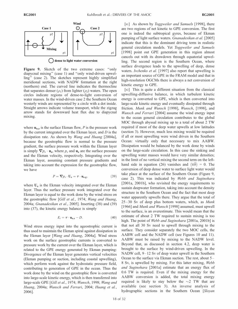
where uo,e is the surface Ekman flow, P is the pressure work
by the current integrated over the Ekman layer, and D is the
dissipation rate. As shown by Wang and Huang [2004a],
because the geostrophic flow is normal to the pressure
gradient, the surface pressure work within the Ekman layer
is simply
#
ps � ue, where ps and ue are the surface pressure
and the Ekman velocity, respectively. Integrating over the
Ekman layer, assuming constant pressure gradients and
taking into account the expression for the geostrophic flow,
we have
P ¼ #
ps � Ue ¼ t � uo;g; ð39Þ
where Ue is the Ekman velocity integrated over the Ekman
layer. Thus the surface pressure work integrated over the
Ekman layer is equal to the work done by the wind stress on
the geostrophic flow [Gill et al., 1974; Wang and Huang,
2004a; Gnanadesikan et al., 2005]. Inserting (38) and (39)
into (37), the kinetic energy balance is simply
Et ¼ t � uo;e � D: ð40Þ
Wind stress energy input into the ageostrophic current is
thus used to maintain the Ekman spiral against dissipation in
the Ekman layer [Wang and Huang, 2004a]. Wind stress
work on the surface geostrophic currents is converted to
pressure work by the current over the Ekman layer, which is
related to the GPE energy generated by Ekman pumping:
Divergence of the Ekman layer generates vertical velocities
(Ekman pumping or suction, including coastal upwelling),
which perform work against the hydrostatic pressure field,
contributing to generation of GPE in the ocean. Thus the
work done by the wind on the geostrophic flow is converted
into large-scale kinetic energy, which is then transferred into
large-scale GPE [Gill et al., 1974; Wunsch, 1998; Wang and
Huang, 2004a; Wunsch and Ferrari, 2004; Huang et al.,
2006].
[81] As shown by Toggweiler and Samuels [1998], there
are two regions of net kinetic to GPE conversion. The first
one is indeed the subtropical gyres, because of Ekman
pumping of light surface waters. Gnanadesikan et al. [2005]
indicate that this is the dominant driving term in realistic
general circulation models. Yet Toggweiler and Samuels
[1998] point out GPE generation in this region almost
cancels out with its drawdown through equatorial upwel-
ling. The second region is the Southern Ocean, where
surface divergence leads to the upwelling of deep, dense
waters. Ivchenko et al. [1997] also report that upwelling is
an important source of GPE in the FRAM model and that in
high-resolution OGCMs there is always a net conversion of
kinetic energy to GPE.
[82] This is quite a different situation from the classical
upwelling-diffusive balance, in which turbulent kinetic
energy is converted to GPE, which is then converted into
large-scale kinetic energy and eventually dissipated through
friction. Munk and Wunsch [1998], Wunsch, [1998], and
Wunsch and Ferrari [2004] assume the wind energy input
to the ocean general circulation contributes to the global
MOC through abyssal mixing up to a total of about 2 TW
required if most of the deep water upwells at low latitudes
(section 3). However, much less mixing would be required
if all or most upwelling were wind driven in the Southern
Ocean: virtually only that necessary to mix AABW.
Dissipation would be balanced by the work done by winds
on the large-scale circulation. In this case the sinking and
upwelling water masses would have very similar densities;
in the limit of no vertical mixing the second term on the left-
hand side in equation (26) vanishes and hwbi = 0. The
conversion of deep dense water to surface light water would
take place at the surface of the Southern Ocean (Figure 9,
case 2). This was indicated by Webb and Suginohara
[2001a, 2001b], who revisited the energy requirements to
sustain deepwater formation, taking into account the density
structure in the Southern Ocean and the fact that most deep
water apparently upwells there. They argue that the total of
25–30 Sv of deep plus bottom waters, which, as Munk
[1966] and Munk and Wunsch [1998] assumed, must upwell
to the surface, is an overestimate. This would mean that the
estimate of about 2 TW required to sustain mixing is too
high. The point of Webb and Suginohara [2001a, 2001b] is
that not all 30 Sv need to upwell through mixing to the
surface. They consider separately the two MOC cells, the
AABW cell and the NADW cell (see Figures 10 and 11).
AABW must be raised by mixing to the NADW level.
Beyond that, as discussed in section 4.2, deep water is
brought to the surface by wind-driven upwelling. In the
NADW cell, 9–12 Sv of deep water upwell in the Southern
Ocean to the surface via Ekman suction. The rest, about 5–
8 Sv, is upwelled by mixing. For this latter mixing, Webb
and Suginohara [2001a] estimate that an energy flux of
0.6 TW is required. Even if the mixing energy for the
AABW conversion is added, the total mixing energy
required is likely to stay below the �2 TW that are
available (see section 3). An inverse analysis of
hydrographic sections in the Southern Ocean [Sloyan
Figure 9. Sketch of the two extreme cases: ‘‘onlydiapycnal mixing’’ (case 1) and ‘‘only wind-driven upwel-ling’’ (case 2). The sketches represent highly simplifiedmeridional sections, with NADW formation at the right(northern) end. The curved line indicates the thermoclinethat separates denser (r1) from lighter (r2) waters. The opencircles indicate regions of dense-to-light conversion ofwater masses. In the wind-driven case 2 the Southern Oceanwesterly winds are represented by a circle with a dot inside.Straight arrows indicate volume transport, while the zigzagarrow stands for downward heat flux due to diapycnalmixing.
RG2001 Kuhlbrodt et al.: DRIVERS OF THE AMOC
18 of 32
RG2001

and Rintoul, 2001a] as well as an analysis of the surface
fluxes [Speer et al., 2000] leads to the same conclusion
that both diapycnal mixing and wind-driven upwelling are
driving the AMOC. The energy budget is closed by
including the required energy input for wind-driven
upwelling.
5. THE ROLE OF DEEP WATER FORMATION
[83] At its surface the ocean exchanges heat, fresh water,
and momentum with the atmosphere. Having discussed the
role of energy and momentum fluxes for the large-scale
circulation in sections 3 and 4, we now concentrate on the
heat (latent, sensible, and radiative) and freshwater (evap-
oration, precipitation, runoff, sea ice, and glacier meltwater)
fluxes that are subsumed as buoyancy fluxes. From Sand-
strom’s theorem (section 2) it is evident that surface buoy-
ancy fluxes cannot provide the energy that is necessary to
drive the AMOC. However, they are essential for deepwater
formation, i.e., the conversion of surface water masses to
deep waters by raising their density through cooling and/or
increasing salinity. The dense deep and bottom water
masses in the oceans are formed in the regions of very high
surface density. In other words, the surface buoyancy fluxes
contribute to setting the properties of the deepwater masses.
While the driving processes set the rate of upwelling of a
steady state MOC, this does not have to result in an inter-
hemispheric overturning circulation in the sense discussed so
far in this review. It is the deepwater formation (DWF)
processes that set the interhemispheric shape and the strength
of the overturning cell. As mentioned in section 4.2, surface
buoyancy fluxes should be considered as necessary for the
existence of a deep MOC in the Atlantic [Huang, 2004].
Figure 10. Schema of the AMOC. The two cells, AABWand NADW, are driven by both diapycnal mixing and wind-driven upwelling. Above the levels of NADWare the lighterIntermediate Waters (IW). Lines indicate isopycnal surfaces;numbers indicate the respective neutral densities. Theneutral density differs only slightly from the potentialdensity but represents isopycnal motions more precisely.See Figure 11 for the observed position of the isopycnals.Other symbols are the same as in Figure 9. For the AABWcell the dense-to-light conversion occurs at depth throughdiapycnal mixing only. For the NADW cell the dense-to-light conversion happens at depth as well as at the surface.For both cells the light-to-dense conversion is due tobuoyancy fluxes and entrainment at high latitudes. Thechoice of the isopycnals is the same as Figure 13 of Sloyanand Rintoul [2001a].
Figure 11. Atlantic south to north cross section of neutral density gn from WOCE data [Schlitzer,2000]. The inset shows the geographical position of the section. Wind-driven upwelling in the SouthernOcean occurs for waters of 27.4 < gn < 28.0 (see Figure 10). AABW, the densest water mass, is found atgn > 28.2. NADW typically has 27.7 < gn < 28.0. In the interior ocean, diapycnal mixing leads to anupwelling of AABW to NADW levels and of part of the NADW to thermocline depth (gn � 27.4). Sincein most cases the underlying data were not observed during the DWF season, the outcropping of therespective isopycnals is not seen here. However, the overflow from Denmark Strait forms a boundarycurrent on the shelf of Greenland at about 1000 m depth, just below the gn = 27.8 isopycnal in thissection.
RG2001 Kuhlbrodt et al.: DRIVERS OF THE AMOC
19 of 32
RG2001

Thus they also strongly determine changes in the NADW
cell of the AMOC, e.g., during the last glacial period
(section 6.1) or, possibly, in the next decades and centuries
(section 6.4).
5.1. Deepwater Formation in the North Atlantic
[84] In the North Atlantic, there are several processes that
lead to DWF. Open ocean deep convection and other
turbulent vertical mixing processes go along with the actual
heat loss to the atmosphere. Salt input occurs when sea ice
freezes because strongly saline water (brine) is released
during this process. Sill overflows, entrainment, and sinking
in the boundary currents are associated with the actual
downward motion.
[85] Open ocean deep convection is observed in the
Labrador Sea and less frequently in the Greenland Sea
[Marshall and Schott, 1999]. It can reach depths of
2000 m in the Labrador Sea and 3000 m in the Greenland
Sea. A deep convection event starts with preconditioning.
Cyclonic wind forcing pushes the surface waters away from
the central Labrador Sea toward the coasts, and this happens
in a comparable way in the Greenland Sea. This surface
divergence leads to upwelling of denser deep waters, which
can be seen in transects as a doming of the isopycnals [Lilly
et al., 1999]. Together with buoyancy loss to the atmo-
sphere, this weakens the vertical density gradient. The
actual convection event is initiated when an individual
weather system results in a strong local heat loss and
removes the remaining weak density stratification in the
ocean. The consequence is a vigorous vertical mixing, with
cold surface waters sinking and warmer deep waters rising.
Such an open ocean convection event occupies and area of
about 50 km diameter and lasts for only a few days. In the
Greenland Sea, brine rejection from sea ice formation
additionally increases the surface layer density. Open ocean
convection also occurs in the Irminger Sea. Yet it is not
established so far whether this plays a role for the AMOC
[Bacon et al., 2003; Pickart et al., 2003].
[86] The net downward motion of waters during a con-
vective event is negligible. After convection, eddies mix the
cold and dense waters in the center of the convection area
with waters in the boundary currents. It is still an open
question where exactly the postconvection sinking occurs.
Recent modeling studies [Spall, 2004; Straneo, 2006]
suggest that the sinking mainly occurs at the lateral
boundaries of the Labrador and Greenland seas. Other
studies suggest that there is an eddy-induced overturning
with sinking in the convection region [Khatiwala et al.,
2002].
[87] While deep convection down to about 2000 m is
necessary for deepwater formation in the Labrador Sea, the
situation in the Nordic Seas is different. Any deepwater
mass circulating from the Nordic Seas into the North Atlantic
has to flow over one of the two sills of the Greenland-Iceland-
Scotland ridge (roughly sketched in Figure 2). Their depths
are 630 m in the Denmark Strait and 840 m in the Faroe
Bank Channel. Hence deepwater formation down to these
depths is sufficient for the necessary buoyancy loss to create
the overflow waters that are involved in the AMOC
[Meincke et al., 1997]. It is observed that these intermediate
depths are ventilated regularly by widespread, wintertime
mixed layer deepening [Watson et al., 1999]. Experiments
indicate that year-round turbulent mixing in the upper
�1000 m is rather strong [Garabato et al., 2004a]. These
processes are associated with strong heat loss of middepth
Atlantic waters. Other relevant processes for DWF are
horizontal eddy mixing, which dilutes the Atlantic Water on
its way north, and shelf convection initiated by brine
release. The freshwater budget of the Nordic Seas is
determined by exchanges with the Arctic Ocean [see, e.g.,
Weaver et al., 1999; Furevik et al., 2007].
[88] Assessing the rates of deep and bottom water for-
mation is a challenging task. Because the very slow vertical
motion of water masses associated with the AMOC eludes
detection even when using modern current meters, there is
no direct way to quantify the amount of water downwelling
at high latitudes. Data on transient tracers such as tritium
(3H), chlorofluorocarbons (CFCs), and others from world-
wide ocean surveys (e.g., Geochemical Ocean Sections
Study, Transient Tracers in the Ocean, and World Ocean
Circulation Experiment) allow an indirect estimate of
NADW formation rate of about 15 ± 2 Sv [Broecker and
Peng, 1982; Ganachaud and Wunsch, 2000]; Talley et al.
[2003] estimate 18 ± 5 Sv from hydrographic data.
[89] The contributions of the different DWF sites to the
total amount of NADW formation are comparable. Esti-
mates of the formation rates are based on direct measure-
ment of the overflow currents [Dickson and Brown, 1994]
and on inference from tracer distributions [Lab Sea Group,
1998; Smethie and Fine, 2001; Khatiwala et al., 2002], with
an error of about 30%: (1) overflow over the Greenland-
Iceland sill in Denmark Strait, 2.4–2.9 Sv; (2) overflow
over the Iceland-Scotland sill, 2.4–2.7 Sv; and (3) DWF in
the Labrador Sea, 2–4 Sv.
[90] To obtain the 15–18 Sv of southward NADW
volume transport, additional processes have to be taken into
account. Notably, entrainment of waters along the currents’
paths adds considerable volume to the sill overflows.
5.2. Deepwater Formation in the Southern Ocean
[91] In contradistinction to the strong convection sites in
the open northern Atlantic the deep water in the Southern
Ocean is formed mainly along the continental slope of
Antarctica. During the winter in the Southern Hemisphere,
large amounts of sea ice are formed around Antarctica.
Because of the rejection of brine they leave behind dense
water masses near the surface. Large ice-free patches in the
sea ice cover, called polynyas, play a central role in this
process also because of strong heat loss [Maqueda et al.,
2004]. The buoyancy loss makes the waters sink to the
bottom of the continental shelf. If the amount is large
enough, it reaches the shelf break and flows down the
continental slope. During this process its volume is
increased significantly by entrainment of less dense waters,
and bottom water is formed [Baines and Condie, 1998].
Specific details of the bottom topography with small spatial
RG2001 Kuhlbrodt et al.: DRIVERS OF THE AMOC
20 of 32
RG2001

structures (on the order of 10 km), such as submarine
canyons, are central to these processes, because they
determine the degree of entrainment of water masses that
is possible because of the roughness of the topography.
Therefore quantitative estimates of the amount of deep
water formed in the Southern Ocean are difficult to obtain.
However, they are crucial for global budgets of the vertical
mass transport, which lead to global estimates of the
required energy that sustains the global overturning
circulation. Interactions between AABW and NADW are
addressed in section 6.3.
[92] Assessments of the AABW formation rate based on
the distribution of D14C and PO*4 give values comparable
with those in the Northern Hemisphere. PO*4 concentrations,
lowest in the North Atlantic (about 0.75 mmol L�1) and
highest in the Southern Ocean (about 1.95 mmol L�1), show
a relatively uniform distribution within the deep Pacific and
Indian oceans with values of about 1.3 mmol L�1. Assuming
northern and southern water masses to be equally well
mixed in these ocean basins, Broecker and Peng [1982]
found a formation rate of southern deep and bottom water of
about 15 Sv. More recent CFC data analyses, however,
contradict these results. Orsi et al. [1999] found that only
about 5 Sv of AABW forms all along Antarctica. To
reconcile these different assessments, Broecker et al. [1999]
assumed the AABW formation rate to be highly variable
during the last 1000 years. They speculate that AABW
formation could have been much higher during the Little Ice
Age (about 16th to 19th century) than today. Orsi et al.
[1999] and Ganachaud and Wunsch [2000] argue that
values derived from CFC and PO*4 are not conflicting
because they refer to different density classes of water
masses. Whereas the PO*4-based value of 15 Sv is
associated with the formation of water masses crossing
the gn = 28.11 isoline below 1500 m, the value of 5 Sv,
derived from CFC data, is associated with production of
waters recently exposed to the atmosphere. Entrainment of
NADW into the relatively freshly formed Antarctic deep
and bottom water coming from the sea surface could explain
the steady increase in the formation rate toward greater
depth. As a consequence they argue that there is no
necessity for the entire amount of 15 Sv of AABW to
upwell to the sea surface. This finding is in line with new
assessments of the global amount of upwelling deepwater
masses. Earlier studies [Munk and Wunsch, 1998] assumed
30 Sv of global deepwater formation, about 15 Sv each from
the northern North Atlantic and the Southern Ocean. More
recently, Webb and Suginohara [2001b] proposed a
maximum amount of 20 Sv that have to reach the sea
surface, as discussed in section 4.
6. STABILITY OF THE AMOC
6.1. Past AMOC Shifts
[93] Analysis of sediment cores and corals provides a
wealth of information on past ocean circulation and shows
that it has undergone major changes during the past
120,000 years (reviewed by Rahmstorf [2002]). Time slice
compilations suggest that at different times, three distinct
circulation modes have prevailed in the Atlantic [Sarnthein
et al., 1994]. These have been labeled the stadial mode,
interstadial mode, and Heinrich mode, based on their
occurrence during stadial (cold) and interstadial (warm)
phases of glacial climate and during Heinrich events (see
below). In the interstadial mode, North Atlantic Deep Water
formed in the Nordic Seas; in the stadial mode it formed in
the subpolar open North Atlantic (i.e., south of Iceland); and
in the Heinrich mode, NADW formation all but ceased, and
waters of Antarctic origin filled the deep Atlantic basin.
This grouping of the data into three distinct modes is a
somewhat subjective interpretation; the data, however,
strongly suggest that latitude shifts of convection (between
the Nordic Seas and the region south of Iceland) have
occurred [e.g., Alley and Clark, 1999] and that at certain
times NADW formation was interrupted [Keigwin et al.,
1994]. There is also solid evidence now for a link between
these ocean circulation changes and abrupt changes in
surface climate [see Clark et al., 2002].
[94] The most dramatic abrupt climate changes are the
Dansgaard-Oeschger (DO) warm events, with a warming
that can exceed 10�C within a decade or so [Severinghaus et
al., 2003]. Proxy data show that the South Atlantic cooled
when the North Atlantic warmed [Voelker et al., 2002],
which is indicative of an ocean heat transport change, and
that salinity in the Irminger Sea increased strongly [van
Kreveld et al., 2000], indicative of saline Atlantic waters
advancing northward.
[95] Another type of abrupt change is the Heinrich
events; sediment data indicate a large discharge of icebergs
into the northern Atlantic [Heinrich, 1988] and a shutdown
of NADW formation [Keigwin et al., 1994]. These events
are thought to have been caused by ice sheet instability; the
iceberg discharge would then have provided a large
freshwater forcing to the Atlantic (of the order of 0.1 Sv
[Hemming, 2004]). This is an important difference to the
DO events, for which no large forcing of the ocean is
known.
[96] At the end of the last glacial period, as the climate
warmed and ice sheets melted, the ocean circulation went
through a number of oscillations that may be explained by
meltwater input, i.e., the Younger Dryas and the 8.2 kyr
cold event.
[97] Many aspects of these abrupt events found in proxy
data have been reproduced in model simulations. Large
freshwater input, such as that associated with Heinrich
events, has been shown in many models to shut down
NADW formation [e.g., Schiller et al., 1997]. While the
earlier attempts to simulate abrupt events were based on
present-day climate states in models, more recently, glacial
climate states have become available as a basis for
simulations of abrupt ocean circulation change [Ganopolski
and Rahmstorf, 2001b]. Latitude shifts in convection can be
triggered by small forcing if the ocean circulation is close to
a threshold; the resulting climate change patterns resemble
DO events [Ganopolski and Rahmstorf, 2001a]. Such
convection shifts could be timed by solar variability [Braun
RG2001 Kuhlbrodt et al.: DRIVERS OF THE AMOC
21 of 32
RG2001

et al., 2005]. The climate response to freshwater input of the
8.2 kyr event has also been simulated with encouraging
results in a number of models [e.g., Bauer et al., 2004].
[98] The variability of the thermohaline ocean circulation
during the Holocene after the 8.2 k event is discussed by
Keigwin and Boyle [2000]. Variations are clearly much
smaller than during glacial times, and the evidence for them
is still controversial and not very strong. An important
question here is whether cooling during the ‘‘Little Ice
Age’’ (�1500–1900 A.D.) is related to THC changes, but
this question remains unresolved.
6.2. Freshwater Fluxes and Bistability
[99] The surface fluxes of fresh water give rise to two
thermohaline feedbacks. The first one is the ‘‘positive salt
advection feedback’’: The AMOC’s NADW cell transports
salt northward, which maintains the waters’ relatively high
salinity in the DWF regions in spite of the freshwater input
in the northern midlatitudes. Because of the higher density
this fosters sinking. Thus there is a positive advective
feedback: An ongoing circulation keeps up the deepwater
formation, and conversely, with a halted NADW formation,
there is no northward salt transport, and hence DWF is
suppressed. This advective feedback was described first by
Stommel [1961] in a simple two-box model. It gives rise to a
parabola-shaped stability diagram that shows a bistability of
the overturning with respect to the atmospheric freshwater
transport (see Figure 12): For a fixed freshwater flux, there
is one stable state with and one stable state without an
overturning circulation. A great number of studies have
followed Stommel’s pioneer work; we mention here, in an
exemplary manner, some studying this or similar box
models [Rooth, 1982; Lohmann and Schneider, 1999;
Monahan, 2002] and some applying it to three-dimensional
ocean and climate models [Bryan, 1986; Marotzke and
Willebrand, 1991; Tziperman et al., 1994; Rahmstorf,
1995a, 1996]. Overviews of this vast field are given by
Weaver and Hughes [1992] and Rahmstorf et al. [1999].
[100] While the basin-size density gradients (see
section 6.3) determine the advective feedback, a second,
‘‘convective’’ feedback concerns one specific deepwater
formation site. There is a net freshwater input at the DWF
sites in the North Atlantic. As long as convection happens
regularly, the inflowing fresh water becomes denser by
mixing with the deep saline waters. This keeps the surface
density high and thus fosters convection to occur in the
following winter. However, once convection has not oc-
curred for a couple of years, because of, e.g., variability in
the surface fluxes, then the fresh water accumulates at the
convection site. This decreases the surface density and
inhibits further convection events. In this way, convection
sites may be switched off. The positive convective feedback
was described in a two-box model by Welander [1982];
many studies since have used it for the analysis of three-
dimensional ocean models [Lenderink and Haarsma, 1994,
1996; Rahmstorf, 1994, 1995b; Pierce et al., 1995] as well
of observed data [Kuhlbrodt et al., 2001].
[101] Both the advective and the convective feedback
imply a possible bistability: Under constant boundary con-
ditions, there can be an ‘‘on’’ and an ‘‘off’’ state. Stommel’s
model for the large-scale MOC assumes that the boxes in
his model are always well mixed, so surface buoyancy
fluxes directly affect the deep flow. We need to reconsider
Stommel’s bistability if wind-driven upwelling (section 4)
plays a major role in driving the MOC.
6.3. Role of the Drivers for the Stability of the AMOC
[102] How do the stability properties of the AMOC
change in dependence on the driving mechanism? How
independent of the driving mechanism is the role of deep-
water formation? We consider here the insight provided by
simple conceptual models based on an equation system that
is analytically solvable and yet is thought to capture the
main physics of the real system. Most of those models
consider a volume flux Y of the AMOC’s NADW cell:
Y / DDr; ð41Þ
where Dr is a meridional density difference and D is the
pycnocline depth or scale of the vertical flow. One of the
first of such conceptual models is the one devised by
Stommel [1961], consisting of a high- and a low-latitude
Figure 12. Schematic stability diagram for the volumeflux of the NADW cell of the AMOC from a modifiedversion of the Stommel [1961] box model. Solid black linesindicate stable equilibrium states, and dotted black linesindicate unstable states. Changing the freshwater flux intothe North Atlantic shifts the position on the branches andmay trigger transitions. These transitions are indicated bylabeled arrows: a, NADW cell spin down due to advectivefeedback; b, shutdown due to the convective feedback;c, transition between different deepwater formation sitesinduced by the convective feedback; and d, restart of theNADW cell. ‘‘S’’ marks the Stommel bifurcation pointbeyond which no North Atlantic Deep Water formation canbe sustained. Adapted from Rahmstorf [2000, Figure 2]with kind permission of Springer Science and BusinessMedia.
RG2001 Kuhlbrodt et al.: DRIVERS OF THE AMOC
22 of 32
RG2001

box whose density difference determines the volume flux of
the NADW cell. This model does not consider the
energetics of the flow. Rather, the AMOC is simply
assumed to be proportional to the meridional density
difference between the boxes, which is determined by the
surface heat and freshwater fluxes and the flow itself.
[103] By contrast, following theories for the structure of
the thermocline, Bryan and Cox [1967] derived a scaling for
the meridional circulation based on geostrophy and on
advective-diffusive heat balance leading to a nonlinear
scaling with the meridional density difference. Their
derivation implies that the vertical scale for the meridional
flow, the depth of the pycnocline, is not fixed as in the
Stommel [1961] framework and that the driving of the
AMOC in the form of diapycnal mixing is explicitly
specified. An equation for the zonal velocity u follows from
thermal wind balance:
f @zu ¼ g
r0@yr: ð42Þ
Inserting typical scales for the pycnocline depth D and the
meridional extent Ly of the flow and with Dr being
the imposed meridional density difference, one obtains for
the zonal flows
U ¼ g
f r0
DrLy
D: ð43Þ
[104] At the base of the thermocline the advection-diffu-
sion balance equation (28) is assumed to hold for the
density. The assumption behind the pycnocline scaling
without wind is that changes in vertical diffusivity only
change the depth of the pycnocline but not the density
difference [Robinson and Stommel, 1959]. Inserting typical
scales into equation 28 provides
D ¼ kv
W: ð44Þ
The relation between meridional and vertical flow is
governed by vorticity dynamics, expressed through the
Sverdrup balance:
bv ¼ f @zw V ¼ f
bW
D: ð45Þ
It is assumed that the zonal flow scales like the meridional
flow, such that ULyD = VLxD. Combining equations (43),
(44), and (45) gives an expression for the meridional
overturning:
Y ¼ VLxD ¼ g f L2x
r0b2
� �1=3
k2=3Dr1=3: ð46Þ
The meridional volume transport is proportional to Dr1/3,and it scales like kv
2/3. Hence this derivation is different from
the scaling in the Stommel box model with a constant
pycnocline depth.
[105] It is important to note that the scaling Y / Dr is the
result of multiple assumptions. One main assumption is that
the pycnocline depth D is determined from advective-
diffusive balance and is also the scale for the volume
transport. However, in the presence of wind forcing, Ekman
pumping creates a ‘‘bowl-shaped’’ structure of the pycno-
cline as consistent with the theories of the ventilated
thermocline and not of vertical mixing. Recently, Marshall
et al. [2002] and Radko and Marshall [2004] suggested that
lateral eddy fluxes rather than the small-scale mixing at the
base of the thermocline are key to maintaining the structure
of the pycnocline and balance the downward transport of
heat through Ekman pumping.
[106] Apart from that, Rahmstorf [1996] noted that
D being independent of the NADW flow rate would be
consistent with NADW not upwelling within the Atlantic.
He obtains a linear relation of the Atlantic overturning with
an interhemispheric meridional density difference in a
global OGCM. Also, his hysteresis curves from the OGCM
follow closely that of an interhemispheric box model related
to the Stommel box model, using a linear scaling with the
density difference. In this model it does not matter by what
mechanism the water upwells (this being outside the model
domain), and the hysteresis behavior is hence independent
of the driving mechanism.
[107] The scaling of equation (46) has been extensively
tested mostly in single-hemisphere models without wind
forcing [Colin de Verdiere, 1988; Marotzke, 1997; Zhang et
al., 1999], as has been reviewed by Park and Bryan [2000].
For the scaling with diffusivity, power laws with exponents
different from 2/3 have been found. Park and Bryan [2000]
attributed discrepancies to a significant amount of spurious
recirculation in the North Atlantic when the overturning is
diagnosed in z coordinates. Park [1999] included the
nonlinear mass transport law into Stommel’s box model
and concluded that this model has different stability
properties.
[108] Another assumption of the scaling equation (46) as
well as for the Stommel-type box models is that since the
meridional density gradient explains only a zonal flow with
geostrophy, it scales like the meridional flow. One common
illustration to underline this assumption is that as the zonal
flow is bounded by continental barriers, it will lead to a
secondary meridional flow: The north-south density differ-
ence leads to an eastward flow, which piles up water that
downwells on the eastern wall. This resulting east-west
gradient in the surface elevation then leads to a northward
flow [Wright et al., 1995].
[109] Marotzke [1997] analytically derived an expression
for the east-west pressure difference and therefore the
meridional flow in relation to the north-south surface
density difference for a one-hemisphere model without wind
forcing and with the assumption that convection takes place
in the eastern boundary. A linear relation between some
measure of the interhemispheric meridional pressure
gradient and the volume flux of the AMOC has been found
diagnostically in global OGCMs. Hughes and Weaver
[1994] used a measure of the depth-integrated baroclinic
RG2001 Kuhlbrodt et al.: DRIVERS OF THE AMOC
23 of 32
RG2001

pressure, defined as the vertical integral of density between
the ocean surface and bottom; Thorpe et al. [2001] took the
density integrated between the surface and 3000 m.
[110] Gnanadesikan [1999] assumed the north-south
pressure difference produces a frictional flow in the western
boundary and through that directly related the meridional
pressure difference to the meridional flow. He extended the
scaling from equation (46) and included two more processes
into the conceptual model that would influence the
pycnocline depth: Southern Ocean winds through the Drake
Passage effect and Southern Ocean eddies. In his frame-
work, northern sinking is balanced by a diffusively driven
upwelling in low latitudes and a wind-driven upwelling in
the Southern Ocean minus an eddy return flow. Hence he
includes the two driving mechanisms explicitly but does not
include the salt advection feedback that could lead to
nonlinear behavior. His model has been under intense
investigation as a possible paradigm for the global MOC
[Saenko and Weaver, 2003; Klinger et al., 2003;
Kamenkovich and Sarachik, 2004]. However, Levermann
and Griesel [2004] discussed that the model does not lead to
a linear scaling with the pressure difference DrD, whichseems contradictory to the diagnostic outcome of OGCMs.
Griesel and Maqueda [2006] showed that a three-
dimensional global OGCM is not consistent with
Gnanadesikan’s [1999] theories, ultimately because the
meridional density difference is not independent of the
driving processes and the pycnocline depth is less variable.
[111] Griesel and Maqueda [2006] show that there is a
linear relation of meridional pressure differences with the
Atlantic overturning for simulations with a global OGCM
for a variety of values of mixing parameters and surface
freshwater forcings. The model behavior is closer to the
Stommel model with linear scaling and an Atlantic
pycnocline that is constant. This is supported by Mignot
et al. [2006], who show that the pycnocline depth is
independent of vertical diffusivity.
[112] The question of how a vertical diffusion coefficient
depending on the stratification influences the AMOC was
addressed by Nilsson and Walin [2001], Nilsson et al.
[2003], and Mohammad and Nilsson [2004]. If the total rate
of mixing energy supply is kept constant, then there is less
vertical mixing in a strongly stratified ocean. In their
conceptual and single-hemisphere models this allows for an
overturning that increases with a decreasing north-south
density gradient in opposition to the Stommel feedback.
This intriguing effect, however, could not be reproduced in
a coupled climate model [Marzeion et al., 2007].
[113] To our knowledge, no conceptual model exists that
would include both driving mechanisms (mixing and winds)
as well as potential processes that lead to nonlinear behavior
in deepwater formation in a realistic way. Keeling [2002] set
up conceptual models of a wind-driven overturning
circulation in the limit of very low diapycnal mixing. In
this framework, there is a bistability for two circulation
states: one with and one without a NADW cell but both with
an AABW cell in the abyssal Atlantic. Yet this bistability
exists only for a narrow parameter range away from the
current climate. Hence these models suggest a stable
AMOC. A very demonstrative analytical model was
constructed by Samelson [2004]. He sees the overturning
circulation as a pump-and-valve system, where the wind-
driven upwelling is the pump and deepwater formation in
high latitudes is the valve. In the case where the buoyancy
fluxes inhibit deepwater formation, then there is a regional
recirculation of the waters pulled up in the Southern Ocean.
While vertical mixing is very weak in both models, they,
nevertheless, clearly demonstrate the difference between the
energy source and the role of the surface buoyancy fluxes.
[114] How does the Stommel bistability depend on the
magnitude of the vertical mixing? In zonally averaged
models [Schmittner and Weaver, 2001; Ganopolski et al.,
2001] the hysteresis loop shrinks with increasing vertical
diffusion. By contrast, Prange et al. [2003] show, in a three-
dimensional ocean model with fixed climatological forcing,
that the Stommel hysteresis increases with vertical mixing
and, conversely, disappears in the limit of no vertical
mixing. It seems that processes like freshwater transports by
the horizontal gyres, while not captured by zonally averaged
models, must be taken into account for determining the
stability.
[115] The wind-driven upwelling mechanism presented
by Toggweiler and Samuels [1993a] has received further
theoretical attention in a series of works [Nof, 2000, 2003;
DeBoer and Nof, 2004a, 2004b]. By taking integrals of the
vertically integrated momentum balance around closed
loops, the vertically integrated pressure gradient terms are
eliminated and the net northward volume inflow into the
North Atlantic is related solely to the Southern Ocean wind
stress. This aspect seems particularly important considering
the consequences for stability of the AMOC. In an ocean
where the overturning circulation would be mainly
determined by Southern Ocean westerlies, deepwater
formation in the North Atlantic would play a more passive
role. If, on the other hand, pressure gradients within the
outflow region in the Southern Ocean can vary over a broad
range independently of the Southern Ocean wind stress,
deepwater formation in the North Atlantic is allowed to vary
more independently, and also a stable off-state can exist.
Indeed, Griesel and Maqueda [2006] show that zonal
pressure gradients in western and eastern boundary currents
in the region of the South Atlantic inflow do play an active
role, independent of Southern Ocean wind stress and
influenced by deepwater formation.
[116] Concerning the relative formation rates of NADW
and AABW, it appears that they are anticorrelated in model
experiments with variations in the buoyancy fluxes [Klinger
and Marotzke, 1999]. In experiments with changes in the
wind stress forcing in the Southern Ocean, however,
NADW strength and AABW strength vary together [Brix
and Gerdes, 2003], although they respond on different
timescales. This latter behavior was corroborated by
Timmermann and Goosse [2004], who, in an experiment
with a coupled ocean-atmosphere model, reduced the global
wind stress to zero and found the ocean to have no global
MOC. The role of wind-driven upwelling for maintaining
RG2001 Kuhlbrodt et al.: DRIVERS OF THE AMOC
24 of 32
RG2001
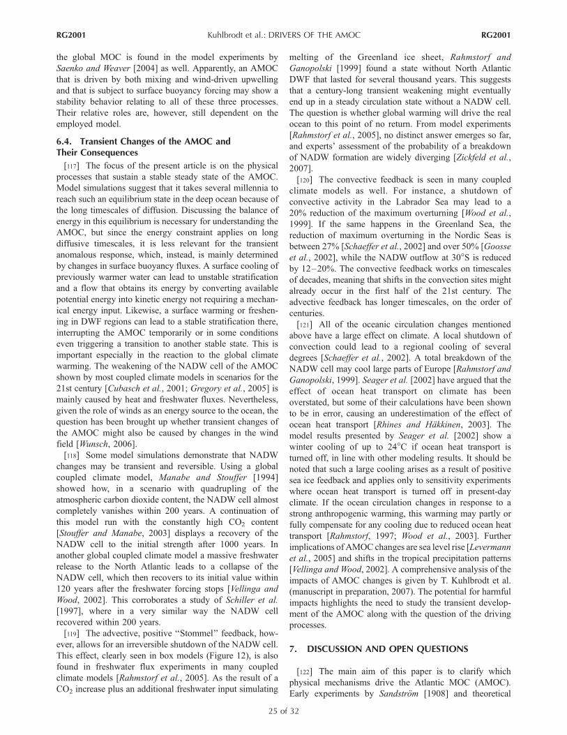
the global MOC is found in the model experiments by
Saenko and Weaver [2004] as well. Apparently, an AMOC
that is driven by both mixing and wind-driven upwelling
and that is subject to surface buoyancy forcing may show a
stability behavior relating to all of these three processes.
Their relative roles are, however, still dependent on the
employed model.
6.4. Transient Changes of the AMOC andTheir Consequences
[117] The focus of the present article is on the physical
processes that sustain a stable steady state of the AMOC.
Model simulations suggest that it takes several millennia to
reach such an equilibrium state in the deep ocean because of
the long timescales of diffusion. Discussing the balance of
energy in this equilibrium is necessary for understanding the
AMOC, but since the energy constraint applies on long
diffusive timescales, it is less relevant for the transient
anomalous response, which, instead, is mainly determined
by changes in surface buoyancy fluxes. A surface cooling of
previously warmer water can lead to unstable stratification
and a flow that obtains its energy by converting available
potential energy into kinetic energy not requiring a mechan-
ical energy input. Likewise, a surface warming or freshen-
ing in DWF regions can lead to a stable stratification there,
interrupting the AMOC temporarily or in some conditions
even triggering a transition to another stable state. This is
important especially in the reaction to the global climate
warming. The weakening of the NADW cell of the AMOC
shown by most coupled climate models in scenarios for the
21st century [Cubasch et al., 2001; Gregory et al., 2005] is
mainly caused by heat and freshwater fluxes. Nevertheless,
given the role of winds as an energy source to the ocean, the
question has been brought up whether transient changes of
the AMOC might also be caused by changes in the wind
field [Wunsch, 2006].
[118] Some model simulations demonstrate that NADW
changes may be transient and reversible. Using a global
coupled climate model, Manabe and Stouffer [1994]
showed how, in a scenario with quadrupling of the
atmospheric carbon dioxide content, the NADW cell almost
completely vanishes within 200 years. A continuation of
this model run with the constantly high CO2 content
[Stouffer and Manabe, 2003] displays a recovery of the
NADW cell to the initial strength after 1000 years. In
another global coupled climate model a massive freshwater
release to the North Atlantic leads to a collapse of the
NADW cell, which then recovers to its initial value within
120 years after the freshwater forcing stops [Vellinga and
Wood, 2002]. This corroborates a study of Schiller et al.
[1997], where in a very similar way the NADW cell
recovered within 200 years.
[119] The advective, positive ‘‘Stommel’’ feedback, how-
ever, allows for an irreversible shutdown of the NADW cell.
This effect, clearly seen in box models (Figure 12), is also
found in freshwater flux experiments in many coupled
climate models [Rahmstorf et al., 2005]. As the result of a
CO2 increase plus an additional freshwater input simulating
melting of the Greenland ice sheet, Rahmstorf and
Ganopolski [1999] found a state without North Atlantic
DWF that lasted for several thousand years. This suggests
that a century-long transient weakening might eventually
end up in a steady circulation state without a NADW cell.
The question is whether global warming will drive the real
ocean to this point of no return. From model experiments
[Rahmstorf et al., 2005], no distinct answer emerges so far,
and experts’ assessment of the probability of a breakdown
of NADW formation are widely diverging [Zickfeld et al.,
2007].
[120] The convective feedback is seen in many coupled
climate models as well. For instance, a shutdown of
convective activity in the Labrador Sea may lead to a
20% reduction of the maximum overturning [Wood et al.,
1999]. If the same happens in the Greenland Sea, the
reduction of maximum overturning in the Nordic Seas is
between 27% [Schaeffer et al., 2002] and over 50% [Goosse
et al., 2002], while the NADW outflow at 30�S is reduced
by 12–20%. The convective feedback works on timescales
of decades, meaning that shifts in the convection sites might
already occur in the first half of the 21st century. The
advective feedback has longer timescales, on the order of
centuries.
[121] All of the oceanic circulation changes mentioned
above have a large effect on climate. A local shutdown of
convection could lead to a regional cooling of several
degrees [Schaeffer et al., 2002]. A total breakdown of the
NADW cell may cool large parts of Europe [Rahmstorf and
Ganopolski, 1999]. Seager et al. [2002] have argued that the
effect of ocean heat transport on climate has been
overstated, but some of their calculations have been shown
to be in error, causing an underestimation of the effect of
ocean heat transport [Rhines and Hakkinen, 2003]. The
model results presented by Seager et al. [2002] show a
winter cooling of up to 24�C if ocean heat transport is
turned off, in line with other modeling results. It should be
noted that such a large cooling arises as a result of positive
sea ice feedback and applies only to sensitivity experiments
where ocean heat transport is turned off in present-day
climate. If the ocean circulation changes in response to a
strong anthropogenic warming, this warming may partly or
fully compensate for any cooling due to reduced ocean heat
transport [Rahmstorf, 1997; Wood et al., 2003]. Further
implications of AMOC changes are sea level rise [Levermann
et al., 2005] and shifts in the tropical precipitation patterns
[Vellinga and Wood, 2002]. A comprehensive analysis of the
impacts of AMOC changes is given by T. Kuhlbrodt et al.
(manuscript in preparation, 2007). The potential for harmful
impacts highlights the need to study the transient develop-
ment of the AMOC along with the question of the driving
processes.
7. DISCUSSION AND OPEN QUESTIONS
[122] The main aim of this paper is to clarify which
physical mechanisms drive the Atlantic MOC (AMOC).
Early experiments by Sandstrom [1908] and theoretical
RG2001 Kuhlbrodt et al.: DRIVERS OF THE AMOC
25 of 32
RG2001

work by Sandstrom [1916] and Bjerknes [1916] suggested
that heating and cooling at the surface alone cannot drive a
deep overturning circulation; rather, a deep heat source is
required for that if other external forcing mechanisms, such
as winds, are absent. Sandstrom was later [e.g., Jeffreys,
1925; Wang and Huang, 2005; Hughes and Griffiths, 2006]
repeatedly challenged on the basis that because of down-
ward mixing of heat (by molecular or turbulent diffusion) a
deep flow can still be sustained even if heating and cooling
occur only at the surface. In our view, however, this
argument still leaves Sandstrom’s fundamental insight
intact. For the large-scale circulation the downward mixing
of heat can be considered as the deep heat source that
Sandstrom’s theorem calls for, and Sandstrom’s insight has
inspired much further work to identify this deep heat (or
buoyancy) source. This is indeed how Sandstrom [1908]
himself saw it when he proposed that downward penetration
of heat in the tropics by mixing could drive the deep flow.
He was incorrect, however, in suggesting that salinity
differences could drive this mixing.
[123] Jeffreys’ [1925] suggestion that turbulent mixing
drives the AMOC was established in detail by Munk and
Wunsch [1998] and Huang [1999]: Turbulent diapycnal
mixing, in balance with slow upwelling, transports heat
downward and thus raises the gravitational potential energy
of the water masses. Molecular diffusion is very likely not
sufficient to obtain a MOC as turbulent and vigorous as
observed [Wang and Huang, 2005]. Paparella and Young
[2002] established that a fluid that is heated and cooled at
the surface only cannot exhibit the kind of turbulence
needed to drive a deep flow if there is no other mechanical
energy source such as winds and tides. Their definition of
turbulence is quite strict; flows could still no longer be
stable and laminar in the regime of an extremely high
Rayleigh number (e.g., for a strong temperature gradient
[Mullarney et al., 2004]). Nevertheless, as pointed out by
Wang and Huang [2005], the amount of mechanical energy
that would be available from surface thermal forcing is only
about 1.5 GW, not enough to explain the circulation
observed in the ocean. A different possible way of raising
the waters from depth is direct wind-driven upwelling
[Toggweiler and Samuels, 1993b, 1995, 1998]. Here heat
fluxes are not directly involved.
[124] Understanding the mechanism that drives the steady
state Atlantic MOC requires understanding its energy
source. There are two main candidates for the driving
mechanisms: (1) mixing, i.e., energy input to small-scale
motion through winds and tides (section 3), and (2) winds,
i.e., direct energy input to the large-scale motion (section 4).
[125] We summarize the past sections by considering the
two extreme cases sketched in Figure 9. If we assume that
large-scale upwelling induced by the surface wind stress is
absent, then upwelling must be in balance with diapycnal
mixing (case 1). The energy source for the turbulent mixing
is internal waves in the ocean that break and dissipate. The
internal waves are triggered by (1) surface winds, (2) inter-
action of tidal waves with the ocean bottom, and (3) the
interaction of eddies with the ocean bottom. These inter-
actions are especially strong where the bottom topography
is rough (underwater ridges, trenches, etc.). However,
considering turbulent mixing as the only driver brings up
a number of questions. The assumption of uniform upwell-
ing leads to estimates of k � 1 � 10�4 m2 s�1 for the
diapycnal mixing coefficient, given the observed present-
day stratification. Yet such large values are not measured
uniformly in the ocean’s interior. In response to these
observations, Munk and Wunsch [1998] reinterpreted their
value of k = 1 � 10�4 m2 s�1 as a basin-wide spatial
average, with values 1 order of magnitude lower in the
ocean interior and much higher values near rough
topography or continental slopes. They estimate that 2
TW mixing energy are necessary to upwell the 30 Sv of
deep waters that are globally formed (section 5). A detailed
energy balance [Munk and Wunsch, 1998; Wunsch and
Ferrari, 2004] (see section 3.2 and Table 1) reveals that the
amount of mixing energy available from the three energy
sources is just 2 TW. There are, however, large uncertainties
in these estimates; thus it is not known whether the energy
budget is really closed.
[126] In the alternative idealized case without diapycnal
mixing (Figure 9, case 2), kinetic energy input is provided
by the winds and is then converted into gravitational poten-
tial energy [Toggweiler and Samuels, 1998; Gnanadesikan et
al., 2005]. In this theory the deep southward flow of North
Atlantic Deep Water is nothing but the return flow of the
surface waters in the Ekman layers in the Southern Ocean
that are pushed northward into the Atlantic [Toggweiler and
Samuels, 1993b, 1995, 1998]. The divergence of the Ekman
transports together with the Drake Passage effect, that
permits no net meridional geostrophic flow in the Southern
Ocean above sill depth, enforces upwelling from depth.
Indeed, the analysis of observed tracer distributions
indicates strong upwelling of water masses in the Southern
Ocean. As can be computed from the curl of the Southern
Ocean wind stress [Doos and Webb, 1994], there are
potentially around 30 Sv of upwelling and subsequent
northward Ekman transport south of 50�S, which can be
regarded as setting a theoretical upper bound to the strength
of the AMOC in the purely wind-driven case. (These 30 Sv
should not be confused with the 30 Sv of global DWF that
Munk and Wunsch [1998] were assuming (section 5).)
However, first, these 30 Sv are partitioned between the
Atlantic and Indo-Pacific oceans; second, the larger part of
the surface volume transport does not reach the North
Atlantic but returns locally at around 40�S; and, third, notall of the upwelling at Drake Passage latitudes originates
from the depth of the NADW outflow. The strength of
Southern Ocean eddies determines how much of the water
returns southward within the Southern Ocean and upwells at
depths shallower than the shallowest sill [Rintoul et al.,
2001]. Thus it is not simply the magnitude of the curl of the
wind stress that determines the amount of Southern Ocean
meridional volume transport that reaches the Atlantic basin.
This volume transport also depends strongly on the density
structure of the Southern Ocean, which is influenced by
eddies and surface heat and freshwater fluxes.
RG2001 Kuhlbrodt et al.: DRIVERS OF THE AMOC
26 of 32
RG2001

[127] The picture that emerges is that of an AMOC driven
by both mixing and wind-driven upwelling [Webb and
Suginohara, 2001a, 2001b; Sloyan and Rintoul, 2001a]. If
we consider the two cells of the AMOC (sketched in
Figures 10 and 11), then AABW is first brought up to the
levels of NADW by mixing and is upwelled from there to
the surface by the wind. By contrast, in the NADW cell, part
of the volume flux is upwelled by the wind, and the rest is
upwelled by diapycnal mixing. Quantitative estimates of the
partition between mixing-driven upwelling and wind-driven
upwelling are still rather rough [Webb and Suginohara,
2001a, 2001b], but the main point here is that, through the
input of large-scale kinetic energy to the large-scale
circulation, less mixing energy is required. Hughes and
Griffiths [2006] argue that the waters that are entrained
downward close to the DWF sites need not upwell to the
surface before and hence can be subtracted from the
mentioned 30 Sv of Munk and Wunsch [1998], and
Gnanadesikan et al. [2005] found that the main source for
gravitational potential energy is the Ekman forcing. In both
cases the required amount of mixing energy is further
reduced.
[128] While this picture seems plausible, there are a
number of issues that need further clarification. In order
to determine the terms in the mixing energy budget more
precisely, from observations, a better understanding of
turbulent mixing in the ocean is needed. The value for the
mixing efficiency g (section 3.2), i.e., the part of the total
turbulent kinetic energy that is available for diapycnal
mixing, is still uncertain. Furthermore, the effectiveness of
this mixing to enhance the potential energy of the system
depends on its location. Mixing drives the overturning as
long as it effectively transports heat (buoyancy) into the
deep ocean. Models suggest that only the mixing in the
thermocline drives a deep overturning (section 3) and that
mixing at the boundaries is more efficient than in the ocean
interior. It still needs to be verified whether locally strong
mixing in regions where the thermocline is close to the
bottom or the slopes (e.g., at the continental shelves) can
account for the required k = 1 � 10�4 m2 s�1 averaged over
the whole ocean volume.
[129] In model simulations the role of diapycnal mixing
should be critically examined with a special focus on the
effective mixing taking place, i.e., including numerical
diffusion. While some models show a realistic AMOC with
a low vertical diffusivity of k = 0.1 � 10�4 m2 s�1, many
ocean models tend to operate on relatively high levels of
vertical diffusivity, since the numerical diffusivity of
advection schemes often is of the same order of magnitude
as the explicitly set one. Moreover, mixing is often used as a
tuning parameter: For example, strong mixing is applied to
strengthen the AMOC and to compensate for deficiencies in
the tracer distribution. As discussed above, this can lead to
an unrealistic balance between the driving mechanisms of
the AMOC and, consequently, to a possibly false represen-
tation of the climatic feedbacks.
[130] If the AMOC is largely wind driven, then this
should imply a strong sensitivity of the AMOC to Southern
Ocean wind forcing. This is, however, not found in all
models [Rahmstorf and England, 1997], and this sensitivity
decreases with increasing model resolution [Hallberg and
Gnanadesikan, 2007], because the regional, eddy-driven
Deacon cell recirculation strengthens.
[131] We have emphasized that surface buoyancy forcing
per se cannot sustain a steady state deep overturning
circulation. However, as discussed in section 6, the distri-
bution of surface heat and freshwater fluxes is linked with
the location of deepwater formation and therefore substan-
tially influences the transient behavior of the overturning.
Evidence from the past as well as model simulations shows
that changes in the surface fluxes can strongly affect the
AMOC, including a general weakening or a reorganization
of the associated current systems, with potentially drastic
climatic impacts (section 6.4). However, the formation
processes of NADW and especially of AABW are not
represented in a satisfying way in most current coupled
climate models. This results in diverging scenarios for
future regional changes of the AMOC. Hence a more
detailed implementation of DWF in models is required.
[132] The stability of the AMOC as portrayed by the
Stommel [1961] bifurcation is still valid for the mixing-
driven part of the AMOC. This includes the sensitivity of
the AMOC to surface buoyancy fluxes. The Stommel
hysteresis loop is reproduced by coupled climate models
[Rahmstorf et al., 2005], and many three-dimensional ocean
models show the linear scaling of the overturning with the
north-south density difference implied by the Stommel
model. Yet, if spurious large mixing coefficients in OGCMs
are reduced, the Stommel hysteresis loop seems to shrink.
For the wind-driven part of the AMOC the role of the
surface fluxes is portrayed by the pump-and-valve concept
of Samelson [2004], where the wind-driven upwelling is the
pump and the surface buoyancy fluxes are the valve.
Shutting the valve in the northern North Atlantic suppresses
DWF there, but the DWF will have to happen elsewhere. If
we assume that the AMOC is driven by diapycnal mixing as
well as by wind-driven upwelling and is subject to surface
buoyancy fluxes, then its stability behavior is determined by
all these processes.
[133] In conclusion, we find that further research about
both the driving processes and the deepwater formation
processes is necessary to understand the AMOC and to
represent it adequately in ocean and climate models.
Beyond the scientific challenge itself these research efforts
are indispensable to reliably assess how the ocean circula-
tion will change in the future and what consequences this
may have for the global climate.
[134] ACKNOWLEDGMENTS. We are grateful to Miguel
A. M. Maqueda for contributing many relevant ideas and for many
discussions from which the paper has gained strongly. We are as
well indebted to Andrey Ganopolski for many useful comments and
suggestions that have improved this manuscript. The paper was
considerably improved by the remarks of Wilbert Weijer and two
anonymous reviewers. The authors appreciate the support of several
funding agencies (T.K., German Federal Ministry for Education,
Science and Research through the project ‘‘Integration’’; A.G. and
RG2001 Kuhlbrodt et al.: DRIVERS OF THE AMOC
27 of 32
RG2001

M.H., McDonnell Foundation; M.M., Spanish Ministry for Science
and Education through the Ramon y Cajal Program and project
CGL2005-06097/CLI; and A.L., Gary Comer Foundation).[135] The Editor responsible for this paper was Henk Dijkstra.
He thanks technical reviewer Wilbert Weijer and two anonymous
reviewers.
REFERENCES
Alford, M. H. (2003), Improved global maps and 54-year historyof wind work on ocean inertial motions, Geophys. Res. Lett.,30(8), 1424, doi:10.1029/2002GL016614.
Alley, R., and P. Clark (1999), The deglaciation of the NorthernHemisphere: A global perspective, Annu. Rev. Earth Planet. Sci.,27, 149–182.
Arneborg, L. (2002), Mixing efficiencies in patchy turbulence,J. Phys. Oceanogr., 32, 1496–1506.
Bacon, S., W. J. Gould, and Y. Jia (2003), Open-ocean convectionin the Irminger Sea, Geophys. Res. Lett., 30(5), 1246,doi:10.1029/2002GL016271.
Baines, P., and S. Condie (1998), Observations and modelling ofAntarctic downslope flows: A review, in Ocean, Ice, and Atmo-sphere: Interactions at the Antarctic Continental Margin,Antarct. Res. Ser., vol. 75, edited by S. S. Jacobs and R. F.Weiss, pp. 29–49, AGU, Washington, D. C.
Bauer, E., A. Ganopolski, and M. Montoya (2004), Simulation ofthe cold climate event 8200 years ago by meltwater outburstfrom Lake Agassiz, Paleoceanography, 19, PA3014,doi:10.1029/2004PA001030.
Beardsley, R. C., and J. F. Festa (1972), A numerical model ofconvection driven by a surface stress and non-uniform horizontalheating, J. Phys. Oceanogr., 2, 444–455.
Bjerknes, V. (1916), Uber thermodynamische Maschinen, die unterMitwirkung der Schwerkraft arbeiten, Abh. Akad. Wissensch.Leipzig, 35(1), 1–33.
Bond, G., et al. (1992), Evidence for massive discharge of icebergsinto the North Atlantic ocean during the last glacial, Nature, 360,245–249.
Braun, H., M. Christl, S. Rahmstorf, A. Ganopolski, A. Mangini,C. Kubatzki, K. Roth, and B. Kromer (2005), Solar forcing ofabrupt glacial climate change in a coupled climate system model,Nature, 438, 208–211.
Brix, H., and R. Gerdes (2003), North Atlantic Deep Water andAntarctic Bottom Water: Their interaction and influence on thevariability of the global ocean circulation, J. Geophys. Res.,108(C2), 3022, doi:10.1029/2002JC001335.
Broecker, W., and T.-H. Peng (1982), Tracers in the Sea, Lamont-Doherty Earth Obs., Palisades, N. Y.
Broecker, W., S. Sutherland, and T. Peng (1999), A possible 20thcentury slowdown of Southern Ocean deep water formation,Science, 286, 1132–1135.
Bryan, F. (1986), High-latitude salinity effects and interhemi-spheric thermohaline circulations, Nature, 323, 301–304.
Bryan, F. (1987), On the parameter sensitivity of primitive equa-tion ocean general circulation models, J. Phys. Oceanogr., 17,970–985.
Bryan, K., and M. Cox (1967), A numerical investigation of theoceanic general circulation, Tellus, 19, 54–80.
Bryan, K., and L. Lewis (1979), A water mass model of the worldocean, J. Geophys. Res., 84, 2503–2518.
Buffoni, G., A. Cappelletti, and P. Picco (2002), An investigationof thermohaline circulation in Terra Nova Bay polynya, Antarct.Sci., 14(1), 83–92.
Caldwell, D., and J. Moum (1995), Turbulence and mixing in theocean, U.S. Natl. Rep. Int. Union Geod. Geophys. 1991–1994,Rev. Geophys., 33, 1385–1394.
Clark, P. U., N. G. Pisias, T. F. Stocker, and A. J. Weaver (2002),The role of the thermohaline circulation in abrupt climatechange, Nature, 415, 863–869.
Colin de Verdiere, A. (1988), Buoyancy driven planetary flows,J. Mar. Res., 46, 215–265.
Colin de Verdiere, A. (1993), On the oceanic thermohaline circula-tion, inModelling Climate-Ocean Interactions, NATO ASI Ser., Ser.I, vol. 12, edited by J. Willebrand and D. Anderson, pp. 151–183, Springer, New York.
Coman, M. A., R. W. Griffiths, and G. O. Hughes (2006), Sand-strom’s experiments revisited, J. Mar. Res., 64, 783–796.
Cubasch, U., et al. (2001), Projections of future climate change, inClimate Change 2001: The Scientific Basis: Contribution ofWorking Group I to the Third Assessment Report of the IPCC,edited by J. T. Houghton et al., chap. 9, pp. 525–582, CambridgeUniv. Press, New York.
Cummins, P., G. Holloway, and A. Gargett (1990), Sensitivity ofthe GFDL ocean general circulation model to a parameterizationof vertical diffusion, J. Phys. Oceanogr., 20, 817–830.
DeBoer, A., and D. Nof (2004a), The Bering Strait’s grip on the North-ern Hemisphere climate, Deep Sea Res., Part I, 51, 1347–1366.
DeBoer, A., and D. Nof (2004b), The exhaust valve of the NorthAtlantic, J. Clim., 17, 417–422.
Defant, A. (1929), Dynamische Ozeanographie, 222 pp., Springer,New York.
Defant, A. (1961), Physical Oceanography, vol. 1, 729 pp.,Elsevier, New York.
Dickson, R. R., and J. Brown (1994), The production of NorthAtlantic Deep Water: Sources, rates and pathways, J. Geophys.Res., 99, 12,319–12,341.
Doos, K., and A. Coward (1997), The Southern Ocean as the majorupwelling zone of North Atlantic Deep Water, Int. WOCENewsl., 27, 3–4.
Doos, K., and D. J. Webb (1994), The Deacon cell and the othermeridional cells of the Southern Ocean, J. Phys. Oceanogr., 24,429–442.
Dutton, J. A. (1986), The Ceaseless Wind: An Introduction to theTheory of Atmospheric Motion, 617 pp., Dover, Mineola, N. Y.
Egbert, G., and R. Ray (2000), Significant dissipation of tidalenergy in the deep ocean inferred from satellite altimeter data,Nature, 405, 775–778.
Faller, A. J. (1968), Sources of energy for the ocean circulation anda theory of the mixed layer, in Proceedings of the Fifth UnitedStates Congress of Applied Mechanics, American Society of Me-chanical Engineers, pp. 651–672, U. of Minn., Minneapolis.
Fofonoff, N. P. (1981), The gulf stream system, in Evolution ofPhysical Oceanography, edited by B. A. Warren and C. Wunsch,pp. 112–139, MIT Press, Cambridge, Mass.
Furevik, T., C. Mauritzen, and R. Ingvaldsen (2007), The flow ofAtlantic Water to the Nordic Seas and Arctic Ocean, in ArcticAlpine Ecosystems and People in a Changing Environment,edited by J. B. Ørbæk et al., Springer, New York.
Gade, H. G., and K. E. Gustafsson (2004), Application of classicalthermodynamical principles to the study of the oceanic overturn-ing circulation, Tellus, Ser. A, 56, 371–386.
Ganachaud, A., and C. Wunsch (2000), Improved estimates ofglobal ocean circulation, heat transport and mixing from hydro-graphic data, Nature, 408, 453–456.
Ganopolski, A., and S. Rahmstorf (2001a), Rapid changes of glacialclimate simulated in a coupled climatemodel,Nature, 409, 153–158.
Ganopolski, A., and S. Rahmstorf (2001b), Stability and variabilityof the thermohaline circulation in the past and future: A studywith a coupled model of intermediate complexity, in TheOceans and Rapid Climate Change: Past, Present, and Future,Geophys. Monogr. Ser., vol. 126, edited by D. Seidov, B. J.Haupt, and M. Maslin, pp. 261–275, AGU, Washington, D. C.
Ganopolski, A., V. Petoukhov, S. Rahmstorf, V. Brovkin,M. Claussen, A. Eliseev, and C. Kubatzki (2001), CLIMBER-2: A climate system model of intermediate complexity. part II:Model sensitivity, Clim. Dyn., 17, 735–751.
Garabato, A. C. N., K. I. C. Oliver, A. J. Watson, and M.-J.Messias (2004a), Turbulent diapycnal mixing in the Nordic Seas,J. Geophys. Res., 109, C12010, doi:10.1029/2004JC002411.
RG2001 Kuhlbrodt et al.: DRIVERS OF THE AMOC
28 of 32
RG2001

Garabato, A. C. N., K. L. Polzin, B. A. King, K. J. Heywood, andM. Visbeck (2004b), Widespread intense turbulent mixing in theSouthern Ocean, Science, 303, 210–213.
Garrett, C., and W. Munk (1972), Space-time scales of internalwaves, Geophys. Astrophys. Fluid Dyn., 2, 225–264.
Garrett, C., and W. Munk (1975), Space-time scales of internalwaves: A progress report, J. Geophys. Res., 80, 291–297.
Garrett, C., and L. St. Laurent (2002), Aspects of deep oceanmixing, J. Phys. Oceanogr., 58, 11–24.
Garrett, C., P. MacCready, and P. Rhines (1993), Boundary mixingand arrested Ekman layers: Rotating stratified flow near a slopingboundary, Annu. Rev. Fluid Mech., 25, 291–323.
Gent, P., and J. McWilliams (1990), Isopycnal mixing in oceancirculation models, J. Phys. Oceanogr., 20, 150–155.
Gerdes, R., C. Koberle, and J. Willebrand (1991), The influence ofnumerical advection schemes on the results of ocean generalcirculation models, Clim. Dyn., 5, 211–226.
Gill, A., S. Green, and A. Simmons (1974), Energy partition in thelarge-scale ocean circulation and the production of mid-oceaneddies, Deep Sea Res. Oceanogr. Abstr., 21, 499–528.
Gill, A. E. (1982), Atmosphere-Ocean Dynamics, 662 pp, Elsevier,New York.
Gnanadesikan, A. (1999), A simple predictive model for the struc-ture of the oceanic pycnocline, Science, 283, 2077–2079.
Gnanadesikan, A., and R. W. Hallberg (2002), Physical oceano-graphy: Thermal structure and general circulation, Encycl. Phys.Sci. Technol., 12, 189–210.
Gnanadesikan, A., and R. J. Toggweiler (1999), Constraints bysilicon cycling on vertical exchange in general circulation mod-els, Geophys. Res. Lett., 26, 1865–1868.
Gnanadesikan, A., R. Slater, P. S. Swath, and G. K. Vallis (2005),The energetics of ocean heat transport, J. Clim., 18, 2604–2616.
Goosse, H., H. Renssen, F. M. Selten, R. J. Haarsma, and J. D.Opsteegh (2002), Potential causes of abrupt climate events: Anumerical study with a three-dimensional climate model, Geo-phys. Res. Lett., 29(18), 1860, doi:10.1029/2002GL014993.
Gregg, M., T. Sanford, and D. Winkel (2003), Reduced mixingfrom the breaking of internal waves in equatorial waters, Nature,422, 513–515.
Gregory, J. M., et al. (2005), A model intercomparison of changesin the Atlantic thermohaline circulation in response to increasingatmospheric CO2 concentration, Geophys. Res. Lett., 32,L12703, doi:10.1029/2005GL023209.
Griesel, A., and M. M. Maqueda (2006), The relation of meridionalpressure gradients to North Atlantic Deep Water volume trans-port in an ocean general circulation model, Clim. Dyn., 26, 781–799.
Griffies, S., R. Pacanowski, and R. Hallberg (2000), Spuriousdiapycnal mixing associated with advection in a z-coordinateocean model, Mon. Weather Rev., 128, 538–564.
Hall, M., and H. Bryden (1982), Direct estimates and mechan-isms of ocean heat transport, Deep Sea Res., Part A, 29, 339–359.
Hallberg, R., and A. Gnanadesikan (2007), The role of eddies indetermining the structure and response of the wind-driven South-ern Hemisphere overturning: Results from the modeling eddiesin the Southern Ocean project, J. Phys. Oceanogr., 36, 2232–2252.
Hasumi, H., and N. Suginohara (1999), Effects of locally enhancedvertical diffusivity over rough bathymetry on the world oceancirculation, J. Geophys. Res., 104(23), 23,367–23,374.
Heinrich, H. (1988), Origin and consequences of cyclic ice raftingin the northeast Atlantic Ocean during the past 130,000 years,Quat. Res., 29, 143–152.
Hemming, S. (2004), Heinrich events: Massive late Pleistocenedetritus layers of the North Atlantic and their global climateimprint, Rev. Geophys., 42, RG1005, doi:10.1029/2003RG000128.
Hofmann, M., and M. Morales-Maqueda (2006), Performance of asecond-order moments advection scheme in an ocean general
circulation model, J. Geophys. Res., 111, C05006,doi:10.1029/2005JC003279.
Hogg, N., and W. Owens (1999), Direct measurement of the deepcirculation within the Brazil Basin, Deep Sea Res., Part II, 46,335–353.
Hogg, N., W. Owens, G. Siedler, and W. Zenk (1996), Circulationin the deep Brazil Basin, in The South Atlantic: Present and PastCirculation, edited by G. Wefer et al., pp. 249–260, Springer,New York.
Holland, W. R. (1975), Energetics of baroclinic oceans, in Numer-ical Models of Ocean Circulation, pp. 168–177, Natl. Acad.Press, Washington, D. C.
Houghton, J. T. (1986), The Physics of Atmospheres, 2nd ed.,Cambridge Univ. Press, New York.
Huang, R. X. (1999), Mixing and energetics of the oceanic thermo-haline circulation, J. Phys. Oceanogr., 29, 727–746. (Corrigen-dum, J. Phys. Oceanogr., 32, 1593, 2002)
Huang, R. X. (2004), Ocean, energy flows, in Encyclopedia ofEnergy, vol. 4, edited by C. J. Cleveland, pp. 497–509, Elsevier,New York.
Huang, R. X., and W. Wang (2003), Gravitational potential energysinks in the oceans, in Near-Boundary Processes and TheirParameterization, Proceedings, ‘Aha Huliko’a Hawaii WinterWorkshop, University of Hawaii at Manoa, January 21–24,2003, edited by P. Muller and D. Henderson, pp. 239–247,Univ. of Hawaii, Manoa.
Huang, R. X., W. Wang, and L. L. Liu (2006), Decadal variabilityof wind energy input into the world ocean, Deep Sea Res., PartII, 53, 31–41.
Hughes, G. O., and R. W. Griffiths (2006), A simple convectivemodel of the global overturning circulation, including effects ofentrainment into sinking regions, Ocean Modell., 12, 46–79.
Hughes, T., and A. Weaver (1994), Multiple equilibria of an asym-metric two-basin model, J. Phys. Oceanogr., 24, 619–637.
Ivchenko, V., A. Treguier, and S. Best (1997), A kinetic energybudget and internal instabilities of the Fine Resolution AntarcticModel, J. Phys. Oceanogr., 27, 5–22.
Jeffreys, H. (1925), On fluid motions produced by differences oftemperature and humidity, Q.J.R. Meteorol. Soc., 51, 347–356.
Jenkins, W. (1980), Tritium and 3He in the Sargasso Sea, J. Mar.Res., 38, 533–569.
Joyce, T. M., and K. G. Speer (1987), Modeling the large-scaleinfluence of geothermal source on abyssal flow, J. Geophys. Res.,92, 2843–2850.
Kamenkovich, I., and E. Sarachik (2004), Mechanisms controllingthe sensitivity of the Atlantic thermohaline circulation to theparameterization of eddy transports in ocean GCMs, J. Phys.Oceanogr., 34, 1628–1647.
Kantha, L., and C. Clayson (2000), Small Scale Processes in Geo-physical Fluid Flows, Int. Geophys. Ser., vol. 67, 888 pp.,Elsevier, New York.
Keeling, R. (2002), On the freshwater forcing of the thermohalinecirculation in the limit of low diapycnal mixing, J. Geophys.Res., 107(C7), 3077, doi:10.1029/2000JC000685.
Keigwin, L., and E. Boyle (2000), Detecting Holocene changes inthermohaline circulation, Proc. Natl. Acad. Sci. U.S.A., 97,1343–1346.
Keigwin, L., W. Curry, S. Lehman, and S. Johnsen (1994), The roleof the deep ocean in North Atlantic climate change between 70and 130 kyr ago, Nature, 371, 323–326.
Key, R., et al. (2004), A global ocean carbon climatology: Resultsfrom the Global Data Analysis Project (GLODAP), Global Bio-geochem. Cycles, 18, GB4031, doi:10.1029/2004GB002247.
Khatiwala, S., P. Schlosser, and M. Visbeck (2002), Rates andmechanisms of water mass transformations in the Labrador Seaas inferred from tracer observations, J. Phys. Oceanogr., 32,666–686.
Killworth, P. D., and M. M. Nanneh (1994), Isopycnic momentumbudget of the Antarctic Circumpolar Current in the Fine Resolu-tion Antarctic Model, J. Phys. Oceanogr., 24, 1201–1223.
RG2001 Kuhlbrodt et al.: DRIVERS OF THE AMOC
29 of 32
RG2001

Klinger, B., S. Drijfhout, J. Marotzke, and J. Scott (2003), Sensi-tivity of basin-wide meridional overturning to diapycnal diffu-sion and remote wind forcing in an idealized Atlantic–SouthernOcean geometry, J. Phys. Oceanogr., 33, 249–266.
Klinger, B. A., and J. Marotzke (1999), Behaviour of double-hemi-sphere thermohaline flows in a single basin, J. Phys. Oceanogr.,29, 382–399.
Kuhlbrodt, T., S. Titz, U. Feudel, and S. Rahmstorf (2001), Asimple model of seasonal open ocean convection. part II: Labra-dor Sea stability and stochastic forcing, Ocean Dyn., 52, 36–49.
Lab Sea Group (1998), The Labrador Sea deep convection experi-ment, Bull. Am. Meteorol. Soc., 79, 2033–2058.
Large, W., J. McWilliams, and S. Doney (1994), Oceanic verticalmixing: A review and a model with a nonlocal boundary layerparameterization, Rev. Geophys., 32(4), 363–403.
Ledwell, J., A. Watson, and C. Law (1993), Evidence for slowmixing across the pycnocline from an open-ocean tracer releaseexperiment, Nature, 364, 701–703.
Ledwell, J., E. Montgomery, K. Polzin, L. St. Laurent, R. Schmitt,and J. Toole (2000), Evidence for enhanced mixing over roughtopography in the abyssal ocean, Nature, 403, 179–182.
Lenderink, G., and R. J. Haarsma (1994), Variability and multipleequilibria of the thermohaline circulation associated with deep-water formation, J. Phys. Oceanogr., 24, 1480–1493.
Lenderink, G., andR. J. Haarsma (1996),Modeling convective transi-tions in the presence of sea ice, J. Phys.Oceanogr., 36, 1448–1467.
Levermann, A., and A. Griesel (2004), Solution of a model for theoceanic pycnocline depth: Scaling of overturning strength andmeridional pressure difference, Geophys. Res. Lett., 31, L17302,doi:10.1029/2004GL020678.
Levermann, A., A. Griesel, M. Hofmann, M. Montoya, andS. Rahmstorf (2005), Dynamic sea level changes following changesin the thermohaline circulation, Clim. Dyn., 24, 347–354.
Levitus, S. (1982), Climatological atlas of the world ocean, Prof.Pap. 13, 173 pp., NOAA, Silver Spring, Md.
Lilly, J. M., P. B. Rhines, M. Visbeck, R. Davis, J. R. N. Lazier,F. Schott, and D. Farmer (1999), Observing deep convection in theLabrador Sea during winter 1994–1995, J. Phys. Oceanogr., 29,2065–2098.
Lohmann, G., and J. Schneider (1999), Dynamics and predictabil-ity of Stommel’s box model: A phase-space perspective withimplications for decadal climate variability, Tellus, Ser. A, 51,326–336.
Lueck, R., and R. Reid (1984), On the production and dissipationof mechanical energy in the ocean, J. Geophys. Res., 89, 3439–3445.
Luyten, J., J. Pedlosky, and H. Stommel (1983), The ventilatedthermocline, J. Phys. Oceanogr., 13, 292–309.
Manabe, S., and R. J. Stouffer (1988), Two stable equilibria of acoupled ocean-atmosphere model, J. Clim., 1, 841–866.
Manabe, S., and R. J. Stouffer (1994), Multiple-century responseof a coupled ocean-atmosphere model to an increase of atmo-spheric carbon dioxide, J. Clim., 7, 5–23.
Maqueda, M., A. Willmott, and N. Biggs (2004), Polynya dy-namics: A review of observations and modeling, Rev. Geophys.,42, RG1004, doi:10.1029/2002RG000116.
Marotzke, J. (1997), Boundary mixing and the dynamics of thethree-dimensional thermohaline circulation, J. Phys. Oceanogr.,27, 1713–1728.
Marotzke, J., and J. Willebrand (1991), Multiple equilibria of theglobal thermohaline circulation, J. Phys. Oceanogr., 21, 1372–1385.
Marshall, J., and F. Schott (1999), Open-ocean convection: Obser-vations, theory, and models, Rev. Geophys., 37(1), 1–64.
Marshall, J., H. Jones, R. Karsten, and R. Wardle (2002), Caneddies set ocean stratification?, J. Phys. Oceanogr., 32, 26–38.
Marzeion, B., A. Levermann, and J. Mignot (2007), The role ofstratification-dependent mixing for the stability of the Atlanticoverturning in a global climate model, J. Phys. Oceanogr., inpress.
McManus, J., R. Francois, J.-M. Gherardi, L. Keigwin, andS. Brown-Leger (2004), Collapse and rapid resumption ofAtlantic meridional circulation linked to deglacial climatechanges, Nature, 428, 834–837.
Meincke, J., B. Rudels, and H. J. Friedrich (1997), The ArcticOcean Nordic Seas thermohaline system, J. Mar. Sci., 54(3),283–299.
Mignot, J., A. Levermann, and A. Griesel (2006), A decompositionof the Atlantic meridional overturning circulation into physicalcomponents using its sensitivity to vertical mixing, J. Phys.Oceanogr., 36, 636–650.
Mohammad, R., and J. Nilsson (2004), The role of diapycnal mix-ing for the equilibrium response of the thermohaline circulation,Ocean Dyn., 54, 54–65.
Monahan, A. H. (2002), Stabilisation by noise of climate regimesin a simple model: Implications for stability of the thermohalinecirculation, J. Phys. Oceanogr., 32, 2072–2085.
Montoya, M., A. Griesel, A. Levermann, J. Mignot, M. Hofmann,A. Ganopolski, and S. Rahmstorf (2005), The Earth systemmodel of intermediate complexity CLIMBER-3a. part I:Description and performance for present day conditions, Clim.Dyn., 25, 237–263.
Morel, A., and D. Antoine (1994), Heating rate within the upperocean in relation to its bio-optical state, J. Phys. Oceanogr., 24,1652–1665.
Moum, J., and T. Osborn (1986), Mixing in the main thermocline,J. Phys. Oceanogr., 16, 1250–1259.
Moum, J., D. Caldwell, J. Nash, and G. Gunderson (2002),Observations of boundary mixing over the continental slope,J. Phys. Oceanogr., 32, 2113–2130.
Mullarney, J. C., R. W. Griffiths, and G. O. Hughes (2004), Con-vection driven by differential heating at a horizontal boundary,J. Fluid Mech., 516, 181–209.
Munk, W. (1966), Abyssal recipes I, Deep Sea Res. Oceanogr.Abstr., 13, 707–730.
Munk, W. (1981), Internal waves and small-scale processes, inEvolution of Physical Oceanography, edited by B. Warren andC. Wunsch, pp. 264–291, MIT Press, Cambridge, Mass.
Munk, W., and C. Wunsch (1998), Abyssal recipes II: Energeticsof tidal and wind mixing, Deep Sea Res., Part I, 45, 1977–2010.
Neumann, G., andW. Pierson (1966), Principles of Physical Ocean-ography, 545 pp., Prentice-Hall, Upper Saddle River, N. J.
Nilsson, J., and G. Walin (2001), Freshwater forcing as a booster ofthe thermohaline circulation, Tellus, Ser. A, 53, 629–641.
Nilsson, J., G. Brostroem, and G. Walin (2003), The thermohalinecirculation and vertical mixing: Does weaker density stratifica-tion give stronger overturning?, J. Phys. Oceanogr., 33, 2781–2795.
Nof, D. (2000), Does the wind control the import and export of theSouth Atlantic?, J. Phys. Oceanogr., 30, 2650–2667.
Nof, D. (2003), The Southern Ocean’s grip on the northward mer-idional flow, Prog. Oceanogr., 56, 223–247.
Oakey, N., B. Ruddick, D. Walsh, and J. Burke (1994), Turbulenceand microstructure measurements during North Atlantic TracerRelease Program, Eos Trans. AGU, 75(3), Ocean Sci. Meet.Suppl., 130.
Oort, A., L. Anderson, and J. Peixoto (1994), Estimates of theenergy cycle of the oceans, J. Geophys. Res., 99, 7665–7688.
Orsi, A., G. Johnson, and J. Bullister (1999), Circulation, mixing,and production of Antarctic Bottom Water, Prog. Oceanogr., 43,55–109.
Osborn, T. (1980), Estimates of the local rate of vertical diffu-sion from dissipation measurements, J. Phys. Oceanogr., 10,83–89.
Paparella, F., and W. R. Young (2002), Horizontal convection isnon-turbulent, J. Fluid Mech., 466, 205–214.
Park, Y.-G. (1999), The stability of thermohaline circulation in atwo-box model, J. Phys. Oceanogr., 29, 3101–3110.
Park, Y.-G., and K. Bryan (2000), Comparison of thermally drivencirculations from a depth-coordinate model and an isopycnal-
RG2001 Kuhlbrodt et al.: DRIVERS OF THE AMOC
30 of 32
RG2001

layer model. part I: Scaling-law sensitivity to vertical diffusivity,J. Phys. Oceanogr., 30, 590–605.
Peltier, W., and C. Caulfield (2003), Mixing efficiency in stratifiedshear flows, Annu. Rev. Fluid Mech., 35, 135–167.
Pickart, R. S., M. A. Spall, M. H. Ribergaard, G. W. K. Moore, andR. F. Milliff (2003), Deep convection in the Irminger Sea forcedby the Greenland tip jet, Nature, 424, 152–156.
Pierce, D. W., T. P. Barnett, and U. Mikolajewicz (1995), Compet-ing roles of heat and freshwater flux in forcing thermohalineoscillations, J. Phys. Oceanogr., 25, 2046–2064.
Polzin, K., J. Toole, J. Ledwell, and R. Schmitt (1997), Spatialvariability of turbulent mixing in the abyssal ocean, Science,276, 93–96.
Prange, M., G. Lohmann, and A. Paul (2003), Influence of verticalmixing on the hysteresis: Analysis of an OGCM, J. Phys. Ocean-ogr., 33, 1707–1721.
Radko, T., and J. Marshall (2004), Eddy-induced diapycnal fluxesand their role in the maintenance of the thermocline, J. Phys.Oceanogr., 34, 372–383.
Rahmstorf, S. (1994), Rapid climate transitions in a coupled ocean-atmosphere model, Nature, 372, 82–85.
Rahmstorf, S. (1995a), Bifurcations of the Atlantic thermohalinecirculation in response to changes in the hydrological cycle,Nature, 378, 145–149.
Rahmstorf, S. (1995b), Multiple convection patterns and thermoha-line flow in an idealized OGCM, J. Clim., 8, 3028–3039.
Rahmstorf, S. (1996), On the freshwater forcing and transport ofthe Atlantic thermohaline circulation, Clim. Dyn., 12, 799–811.
Rahmstorf, S. (1997), Risk of sea-change in the Atlantic, Nature,388, 825–826.
Rahmstorf, S. (2000), The thermohaline ocean circulation: Asystem with dangerous thresholds?, Clim. Change, 46, 247–256.
Rahmstorf, S. (2002), Ocean circulation and climate during thepast 120,000 years, Nature, 419, 207–214.
Rahmstorf, S. (2003), Thermohaline circulation: The current cli-mate, Nature, 421, 699.
Rahmstorf, S., and M. England (1997), Influence of SouthernHemisphere winds on North Atlantic Deep Water flow, J. Phys.Oceanogr., 27, 2040–2054.
Rahmstorf, S., and A. Ganopolski (1999), Long-term global warm-ing scenarios computed with an efficient coupled climate model,Clim. Change, 43, 353–367.
Rahmstorf, S., J. Marotzke, and J. Willebrand (1999), Stability ofthe thermohaline circulation, in The Warm Water Sphere of theNorth Atlantic Ocean, edited by W. Krauss, pp. 129–158,Gebruder Borntraeger, Stuttgart, Germany.
Rahmstorf, S., et al. (2005), Thermohaline circulation hysteresis: Amodel intercomparison, Geophys. Res. Lett., 32, L23605,doi:10.1029/2005GL023655.
Redi, M. (1982), Oceanic isopycnal mixing by coordinate rotation,J. Phys. Oceanogr., 12, 1154–1158.
Rhines, P. B., and S. Hakkinen (2003), Is the oceanic heat transportin the North Atlantic irrelevant to the climate in Europe?, Arct.Subarct. Ocean Fluxes Newsl., 1, 13–17.
Rintoul, S. R., C. W. Hughes, and D. Olbers (2001), The AntarcticCircumpolar Current system, in Ocean Circulation and Climate,edited by G. Siedler, pp. 271–301, Elsevier, New York.
Robbins, P. E., and J. M. Toole (1997), The dissolved silica budgetas a constraint on the meridional overturning circulation of theIndian Ocean, Deep Sea Res., Part I, 44, 879–906.
Robinson, A., and H. Stommel (1959), The oceanic thermoclineand the associated thermohaline circulation, Tellus, 3, 295–308.
Rooth, C. (1982), Hydrology and ocean circulation, Prog. Ocea-nogr., 11, 131–149.
Rossby, H. T. (1965), On thermal convection driven by non-uni-form heating from below, Deep Sea Res. Oceanogr. Abstr., 12,9–16.
Rossby, T. (1998), Numerical experiments with a fluid heated non-uniformly from below, Tellus, Ser. A, 50, 242–257.
Saenko, O., and W. Merryfield (2005), On the effect of topogra-phically enhanced mixing on the global ocean circulation,J. Phys. Oceanogr., 35, 826–834.
Saenko, O., and A. Weaver (2003), Southern Ocean upwelling andeddies: Sensitivity of the global overturning to the surface den-sity range, Tellus, Ser. A, 55, 106–111.
Saenko, O. A., and A. J. Weaver (2004), What drives heat transportin the Atlantic Ocean?, Geophys. Res. Lett., 31, L20305,doi:10.1029/2004GL020671.
Samelson, R. (2004), Simple mechanistic models of middepth mer-idional overturning, J. Phys. Oceanogr., 34, 2096–2103.
Sandstrom, J. W. (1908), Dynamische Versuche mit Meerwasser,Ann. Hydrogr. Mar. Meteorol., 36, 6–23.
Sandstrom, J. W. (1916), Meteorologische Studien im Schwe-dischen Hochgebirge, Goteborgs K. Vetensk. VitterhetssamhalletsHandkl., 27, 48 pp.
Sarnthein, M., K. Winn, S. J. A. Jung, J.-C. Duplessy, L. Labeyrie,H. Erlenkeuser, and G. Ganssen (1994), Changes in east Atlanticdeepwater circulation over the last 30,000 years: Eight time slicereconstructions, Paleoceanography, 9, 209–267.
Schaeffer, M., F. M. Selten, J. D. Opsteegh, and H. Goosse (2002),Intrinsic limits to predictability of abrupt regional climate changein IPCC SRES scenarios, Geophys. Res. Lett., 29(16), 1767,doi:10.1029/2002GL015254.
Schiller, A., U. Mikolajewicz, and R. Voss (1997), The stability ofthe North Atlantic thermohaline circulation in a coupled ocean-atmosphere general circulation model, Clim. Dyn., 13, 325–347.
Schlitzer, R. (2000), Electronic atlas of WOCE hydrographic andtracer data now available, Eos Trans. AGU, 81(5), 45.
Schmitt, R. W. (1994), Double diffusion in oceanography, Annu.Rev. Fluid Mech., 26, 255–285.
Schmittner, A. (2005), Decline of the marine ecosystem caused bya reduction in the Atlantic overturning circulation, Nature, 434,628–633.
Schmittner, A., and A. Weaver (2001), Dependence of multipleclimate states on ocean mixing parameters, Geophys. Res. Lett.,28, 1027–1030.
Schmitz, W. J. (1995), On the interbasin-scale thermohaline circu-lation, Rev. Geophys., 33(2), 151–174.
Schmitz, W. J. (1996), On the world ocean circulation, vol. II: ThePacific and Indian Oceans: A global update, Tech. Rep., WHOI-96-08, 237 pp., Woods Hole Oceanogr. Inst., Woods Hole, Mass.
Scott, J. R., and J. Marotzke (2002), The location of diapycnalmixing and the meridional overturning circulation, J. Phys.Oceanogr., 32, 3578–3595.
Seager, R., D. S. Battisti, J. Yin, N. Gordon, N. Naik, A. C.Clement, and M. A. Cane (2002), Is the Gulf Stream respon-sible for Europe’s mild winters?, Q. J. R. Meteorol. Soc., 128,1–24.
Severinghaus, J. P., et al. (2003), A method for precise measure-ment of argon 40/36 and krypton/argon ratios in trapped air inpolar ice with applications to past firn thickness and abrupt cli-mate change in Greenland and at Siple Dome, Antarctica, Geo-chim. Cosmochim. Acta, 67, 325–343.
Siggers, J. H., R. R. Kershwell, and N. J. Balmforth (2004),Bounds on horizontal convection, J. Fluid Mech., 517, 55–70.
Simmons, H., S. Jayne, L. St. Laurent, and A. Weaver (2004),Tidally driven mixing in a numerical model of the ocean generalcirculation, Ocean Modell., 6, 245–263.
Sloyan, B. M., and S. R. Rintoul (2001a), The Southern Oceanlimb of the global deep overturning circulation, J. Phys. Ocea-nogr., 31, 143–173.
Sloyan, B. M., and S. R. Rintoul (2001b), Circulation, renewal andmodification of Antarctic mode and intermediate water, J. Phys.Oceanogr., 31, 1005–1030.
Smethie, W. M., Jr., and R. A. Fine (2001), Rates of North AtlanticDeep Water formation calculated from chlorofluorocarbon inven-tories, Deep Sea Res., Part I, 48, 189–215.
Spall, M. J. (2004), Boundary currents and watermass transforma-tion in marginal seas, J. Phys. Oceanogr., 34, 1197–1213.
RG2001 Kuhlbrodt et al.: DRIVERS OF THE AMOC
31 of 32
RG2001
Speer, K., S. Rintoul, and B. Sloyan (2000), The diabatic Deaconcell, J. Phys. Oceanogr., 30, 3212–3222.
St. Laurent, L., and C. Garrett (2002), The role of internal tides inmixing the deep ocean, J. Phys. Oceanogr., 32, 2882–2899.
Stommel, H. (1961), Thermohaline convection with two stableregimes of flow, Tellus, 13, 224–230.
Stommel, H. (1962), On the smallness of sinking regions in theocean, Proc. Natl. Acad. Sci. U.S.A., 48, 766–772.
Stommel, H., and A. B. Arons (1960), On the abyssal circulation ofthe world ocean - I. Stationary planetary flow patterns on asphere, Deep Sea Res., 6, 140–154.
Stouffer, R. J., and S. Manabe (2003), Equilibrium response ofthermohaline circulation to large changes in atmospheric CO2,Clim. Dyn., 20, 759–773, doi:10.1007/s00382-002-0302-4.
Straneo, F. (2006), On the connection between dense water forma-tion, overturning and poleward heat transport in a convectivebasin, J. Phys. Oceanogr., 36, 1822–1840.
Talley, L., J. Reid, and P. Robbins (2003), Data-basedmeridional over-turning streamfunctions for the global ocean, J. Clim., 16, 3213–3224.
Thompson, L., and G. Johnson (1996), Abyssal currents generatedby diffusion and geothermal heating over rises, Deep Sea Res.,Part I, 43, 193–211.
Thorpe, R., J. Gregory, T. Johns, R. Wood, and J. Mitchell (2001),Mechanisms determining the Atlantic thermohaline circulationresponse to greenhouse gas forcing in a non-flux-adjustedcoupled climate model, J. Clim., 14, 3102–3116.
Timmermann, A., and H. Goosse (2004), Is the wind stress forcingessential for the meridional overturning circulation?, Geophys.Res. Lett., 31, L04303, doi:10.1029/2003GL018777.
Timmermann, A., S.-I. An, U. Krebs, and H. Goosse (2005),ENSO suppression due to weakening of the North Atlantic ther-mohaline circulation, J. Clim., 18, 2842–2859.
Toggweiler, J. R., and B. Samuels (1993a), Is the magnitude of thedeep outflow from the Atlantic Ocean actually governed bySouthern Hemisphere winds?, in The Global Carbon Cycle,NATO ASI Ser., Ser. I, edited by M. Heimann, pp. 333–366,Springer, New York.
Toggweiler, J. R., and B. Samuels (1993b), New radiocarbonconstraints on the upwelling of abyssal water to the ocean’ssurface, in The Global Carbon Cycle., NATO ASI Ser., Ser. I,edited by M. Heimann, pp. 303–331, Springer, New York.
Toggweiler, J. R., and B. Samuels (1995), Effect of Drake Passageon the global thermohaline circulation, Deep Sea Res., Part I, 42,477–500.
Toggweiler, J. R., and B. Samuels (1998), On the ocean’s largescale circulation in the limit of no vertical mixing, J. Phys.Oceanogr., 28, 1832–1852.
Toggweiler, J. R., K. Dixon, and W. S. Broecker (1991), The Peruupwelling and the ventilation of the South Pacific thermocline,J. Geophys. Res., 96, 20,467–20,497.
Trenberth, K. E., and J. M. Caron (2001), Estimates of meridionalatmosphere and ocean heat transports, J. Clim., 14, 3433–3443.
Tziperman, E., J. R. Toggweiler, Y. Feliks, and K. Bryan (1994),Instability of the thermohaline circulation with respect to mixedboundary conditions: Is it really a problem for realistic models?,J. Phys. Oceanogr., 24, 217–232.
Vallis, G. (1999), Large-scale circulation and production of strati-fication: Effects of wind, geometry and diffusion, J. Phys. Ocea-nogr., 30, 933–954.
van Kreveld, S., M. Sarnthein, H. Erlenkeuser, P. Grootes, S. Jung,M. J. Nadeau, U. Pflaumann, and A. Voelker (2000), Potentiallinks between surging ice sheets, circulation changes, and theDansgaard-Oeschger cycles in the Irminger Sea, 60–18 kyr,Paleoceanography, 15, 425–442.
Vellinga, M., and R. A. Wood (2002), Global climatic impacts of acollapse of the Atlantic thermohaline circulation, Clim. Change,54, 251–267.
Veronis, G. (1975), The role of models in tracer studies, in Numer-ical Models of Ocean Circulation, pp. 133–146, Natl. Acad. ofSci., Washington, D. C.
Voelker, A., et al. (2002), Global distribution of centennial-scalerecords for marine isotope stage (MIS) 3: A database, Quat. Sci.Rev., 21, 1185–1214.
Wang, W., and R. X. Huang (2004a), Wind energy input into theEkman layer, J. Phys. Oceanogr., 34, 1267–1275.
Wang, W., and R. X. Huang (2004b), Wind energy input into thesurface waves, J. Phys. Oceanogr., 34, 1276–1280.
Wang, W., and R. X. Huang (2005), An experimental study onthermal circulation driven by horizontal differential heating,J. Fluid Mech., 540, 49–73.
Watanabe, M., and T. Hibiya (2002), Global estimates of the wind-induced energy flux to inertial motions in the surface mixedlayer, Geophys. Res. Lett., 29(8), 1239, doi:10.1029/2001GL014422.
Watson, A. J., et al. (1999), Mixing and convection in the Green-land Sea from a tracer-release experiment, Nature, 401, 902–904.
Weaver, A. J., and T. M. C. Hughes (1992), Stability and varia-bility of the thermohaline circulation and its link to climate, inTrends in Physical Oceanography, pp. 15–70, Counc. of Sci.Res. Integr., Trivandrum, India.
Weaver, A. J., C. M. Bitz, A. F. Fanning, and M. M. Holland(1999), Thermohaline circulation: High-latitude phenomena andthe difference between the Pacific and Atlantic, Annu. Rev. EarthPlanet. Sci., 27, 231–285.
Webb, D. J., and N. Suginohara (2001a), Vertical mixing in theocean, Nature, 409, 37.
Webb, D. J., and N. Suginohara (2001b), The interior circulation ofthe ocean, inOcean Circulation and Climate, edited by G. Siedler,pp. 205–214, Elsevier, New York.
Welander, P. (1982), A simple heat-salt oscillator, Dyn. Atmos.Oceans, 6, 233–242.
Wood, R. A., A. B. Keen, J. F. B. Mitchell, and J. M. Gregory(1999), Changing spatial structure of the thermohaline circulationin response to atmospheric CO2 forcing in a climate model,Nature, 399, 572–575.
Wood, R. A., M. Vellinga, and R. Thorpe (2003), Global warm-ing and thermohaline circulation stability, Philos. Trans. R. Soc.London, Ser. A, 361, 1961–1975.
Wright, D., C. Vreugdenhil, and T. Hughes (1995), Vorticitydynamics and zonally averaged ocean circulation models,J. Phys. Oceanogr., 25, 2141–2154.
Wunsch, C. (1998), The work done by the wind on the oceanicgeneral circulation, J. Phys. Oceanogr., 28, 2332–2340.
Wunsch, C. (2005), Thermohaline loops, Stommel box models,and the Sandstrom theorem, Tellus, Ser. A, 57, 84–99.
Wunsch, C. (2006), Abrupt climate change: An alternative view,Quat. Res., 65, 191–203.
Wunsch, C., and R. Ferrari (2004), Vertical mixing, energy and thegeneral circulation of the oceans, Annu. Rev. Fluid Mech., 36,281–314.
Wunsch, C., D. Hu, and B. Grant (1983), Mass, heat, salt andnutrient fluxes in the South Pacific Ocean, J. Phys. Oceanogr.,13, 725–753.
Zhang, J., R. Schmitt, and R. Huang (1999), The relative influenceof diapycnal mixing and hydrologic forcing on the stability of thethermohaline circulation, J. Phys. Oceanogr., 29, 1096–1108.
Zickfeld, K., A. Levermann, M. Granger Morgan, T. Kuhlbrodt,S. Rahmstorf, and D. Keith (2007), Expert judgements on theresponse of the Atlantic meridional overturning circulation toclimate change, Clim. Change, in press.
�������������������������A. Griesel, Scripps Institution of Oceanography, La Jolla, CA, USA.M. Hofmann, T. Kuhlbrodt, A. Levermann, and S. Rahmstorf,
Climate System Department, Potsdam Institute for Climate ImpactResearch, P.O. Box 601203, D-14412 Potsdam, Germany. ([email protected])M. Montoya, Departamento Astrofisica y Ciencias de la Atmosfera,
Facultad de Ciencias Fısicas, Universidad Complutense de Madrid,28040 Madrid, Spain.
RG2001 Kuhlbrodt et al.: DRIVERS OF THE AMOC
32 of 32
RG2001