QEDQueen’s Economics Department Working Paper No. 1315

Reworking Wild Bootstrap Based Inference for ClusteredErrors

Matthew D. WebbUniversity of Calgary

Department of EconomicsQueen’s University

94 University AvenueKingston, Ontario, Canada

K7L 3N6

11-2014

Reworking Wild Bootstrap Based Inference for

Clustered Errors

Matthew D. Webb∗

November 13, 2014

Abstract

Many empirical projects involve estimation with clustered data. While esti-

mation is straightforward, reliable inference can be challenging. Past research

has suggested a number of bootstrap procedures when there are few clusters. I

demonstrate, using Monte Carlo experiments, that these bootstrap procedures

perform poorly with fewer than eleven clusters. With few clusters, the wild

cluster bootstrap results in p-values that are not point identi�ed. I suggest

two alternative wild bootstrap procedures. Monte Carlo simulations provide

evidence that a 6-point bootstrap weight distribution improves the reliability of

inference. A brief empirical example concerning education tax credits highlights

the implications of these �ndings.

JEL:C15, C21, C23Keywords:CRVE, grouped data, clustered data, panel data, wild cluster bootstrap

∗Department of Economics, University of Calgary, Calgary, Alberta, Canada, T2N 1N4. Email:mwebb@ucalgary.ca. I thank my supervisors, James MacKinnon and Steven Lehrer, for their con-tinued support. I am grateful to Michele Campolieti, Marco Cozzi, Allan Gregory, and anonymousreferees for thoughtful evaluations on a prior draft. I would also like to thank Russell Davidson,Jonah Gelbach, Emmanuel Flachaire, Maximilien Ka�o Melou, and Arthur Sweetman for helpfulcomments and suggestions. I am grateful to participants at the 47th Canadian Economics Associa-tion Conference, the 8th CIREQ Ph.D. Student Conference, the 29th Canadian Econometric StudyGroup Annual Meeting, and seminar participants at the University of Calgary, Université du Québecà Montréal, Wilfrid Laurier University, and Ryerson University.

1

1 Introduction

Research often involves controlling for dependence within clusters. Clusters can be

regarded as a natural grouping of observations. Common examples of clusters are

students within classrooms, �rms within industries, and individuals within states.

When the data are clustered OLS or `robust' means of inference are quite unreliable.

This problem occurs whenever there is strong correlation of independent variables

or error terms within a cluster or group. It is most severe whenever an independent

variable is invariant within a cluster, as discussed in Moulton (1990). A very thorough

survey is provided by Cameron and Miller (2014).

Issues of within cluster dependence have been of concern to applied researchers for

quite sometime, and packages such as Stata's `cluster' command are now common-

place within statistical analysis packages.1 These packages implement Cluster Robust

Variance Estimator (CRVE) routines and often work very well. However, problems

can occur when the data under analysis fail to meet the asymptotic requirements of

the CRVE. This frequently occurs when there are a small number of clusters in the

dataset, a result known since Bertrand, Du�o and Mullainathan (2004) (BDM) and

Donald and Lang (2007). With few clusters, the CRVE can result in p-values that

are, on average, too small resulting in type I errors occurring too frequently.

A common correction for the small clusters problem is to use a wild cluster boot-

strap, due to Cameron, Gelbach and Miller (2008) (CGM).2 This technique works

very well with an intermediate number of clusters; however, this paper demonstrates

that with few clusters the procedure results in p-values that are not point identi�ed.

The appropriateness of the conventional wild cluster bootstrap increases with the

number of clusters. Yet, there are many real world problems where data sets contain

few clusters. For example, policy analysts in Australia and Canada often exploit vari-

ation across eight or ten regions, while others exploit variation between and within

regions in the United States. Alternatively, following Thompson (2011) clustering is

often accounted for in the time dimension, and many panel data sets have few time

periods.

This paper suggests two procedures when working with few clusters, considering

1Rogers (1994) implemented cluster robust inference within Stata and has over 1980 citationsaccording to Google Scholar as of September, 2014.

2Cameron, Gelbach and Miller (2008) has over 670 citations according to Google Scholar as ofSeptember, 2014.

2

both enumerating the bootstrap samples and alternative bootstrap weight distribu-

tions. Enumeration involves systematically calculating all of the possible bootstrap

samples, and their associated t-statistics. Expanding the 2-point wild cluster boot-

strap to a 6-point distribution appears to perform well, even in settings with �ve

clusters.

Section 2 of this paper discusses the limitations of the 2-point wild cluster boot-

strap. Alternative bootstrap methods to account for the few clusters problem are

considered in section 3. Section 4 addresses the design and results of Monte Carlo

simulations which expose the limitations of existing techniques when properly calcu-

lated, and favor a new 6-point distribution. A brief empirical example applies these

procedures to an analysis of education related tax credits in section 5 and section 6

concludes.

2 Background onMethods to Deal WithWithin Clus-

ter Correlation

A data set can be considered clustered when there is a natural grouping of the obser-

vations. A common correction for clustered errors is to estimate standard errors using

a Cluster Robust Variance Estimator (CRVE).3 General results in White (1984) on

covariance matrix estimation imply the consistency of this estimator based on three

assumptions:

A1. The number of clusters, G, goes to in�nity.

A2. The degree of within-cluster correlation is constant across clusters.

A3. Each cluster contains an equal number of observations.

Several authors have previously studied the performance of the CRVE when G is

small. Simulation results from Bertrand, Du�o and Mullainathan (2004) and others

show that with 6 clusters CRVE rejection rates can be several times the desired size.4

BDM propose a block bootstrap procedure as a means of improving test sizes, and

3Kloek (1981) identi�ed the problem of constant regressors within grouped data, though it waspopularized by Liang and Zeger (1986), Moulton (1990), and Rogers (1994). The problem wasconsidered in the Di�erence-in-Di�erences context by Bertrand, Du�o and Mullainathan (2004) andDonald and Lang (2007). Recent work has been done by Ibragimov and Muller (2010), Imbensand Kolesar (2012) and Brewer, Crossley and Joyce (2013). For a detailed survey on cluster robustinference see Cameron and Miller (2014).

4Carter, Schnepel and Steigerwald (2013) relax assumptions A2 and A3 and derive a new asymp-totic distribution for the test statistic. Imbens and Kolesar (2012) also deal with violations of A3.MacKinnon and Webb (2014) study the �nite sample properties when A3 is violated.

3

CGM suggest that with fewer than 30 clusters, the block bootstrap rejection rate is

too large. CGM propose the wild cluster bootstrap, a variant of the wild bootstrap

due to Wu (1986).5 The wild cluster bootstrap has many desirable features: each and

every observation in the original dataset is in each bootstrap sample exactly once,

and the structure of the error correlation within clusters is preserved. The procedure

for the wild cluster bootstrap is as follows. First consider the OLS regression model:

Yig = β0 + β1Xig + uig. (1)

Imagine we are interested in calculating a wild cluster bootstrap-t p-value for β1 in

equation (1). We can construct the p-value by �rst estimating the t-statistic, t, in

the original sample using cluster-robust standard errors. We then re-estimate the

equation by imposing the null hypothesis, to obtain the restricted estimates β0, β1,

uig. Then B iterations, or bootstraps, are performed. In each iteration a bootstrap

sample is generated from the bootstrap data generating process

y∗ig = β0 + β1Xig + uigvg, (2)

where the ith residual in group g, uig, is multiplied by the bootstrap weight vg. In

general the bootstrap DGP should impose the null hypothesis, which in this case

would mean setting β1 = 0.

The di�erence between the wild cluster bootstrap and the conventional wild boot-

strap is that under the former the same vg is applied to all observations within the

same cluster, while the conventional wild bootstrap applies a vig to each observation.

The bootstrap weight can take many forms. In each iteration, a bootstrap t-statistic

t∗j is generated using cluster-robust standard errors. After B iterations the bootstrap

p-value is then calculated by:

p∗(t) = 2 min

(1

B

B∑j=1

I(t∗j ≤ t

),1

B

B∑j=1

I(t∗j > t

)), (3)

where I(.) is the standard indicator function.6

5MacKinnon and Webb (2014) propose using the wild cluster bootstrap for clusters of unequalsize. Hagemann (2014) proposes a wild cluster bootstrap for quantile regression.

6These p-values are equal tail p-values, while the enumeration p-values are symmetric p-valuescalculated by (1/B)

∑Bj=1 I(|t∗j | >= |t|).

4

Simplifying, the DGP generates unique bootstrap samples solely as a function

of the transformed residuals. This procedure is based on the assumption that B

bootstrap samples, are drawn from an extremely large pool of potential bootstrap

samples. Inference on β depends on where t falls in the sorted vector of bootstrap

t-statistics, t∗ = t∗1, ..., t∗B. If our estimated t-statistic falls between the 90th and 91st

bootstrap t-statistic, then the p-value of this t-statistic is 0.180. When there is a large

number of potential samples, the generated set of bootstrap samples will contain few,

if any, repeated samples. Accordingly, the location of t can be precisely identi�ed,

and the resulting p-value is point identi�ed.

CGM present evidence that the wild cluster bootstrap-t method is preferable to

several alternative bootstrap methods, and allows for reliable inference with as few

as �ve clusters. However, when the number of clusters is small, so is the number of

unique bootstrap samples for the method advocated by CGM. As I now show, this

makes reliable inference di�cult. With few clusters, the number of unique potential

bootstrap samples is rather small, as bootstrap samples depend on the choice of a

bootstrap weight distribution. Two well-known distributions are the Rademacher and

the Mammen, both of which contain only two points. With these distributions, vg

from equation (2) is set to one of two values with a given probability, p.7

Cameron, Gelbach and Miller (2008) recommend the Rademacher weights, as do

Davidson, Monticini and Peel (2007) and Davidson and Flachaire (2008). Accordingly,

there are only 2G possible bootstrap samples, where G is the number of groups. The

number of unique absolute value t-statistics is only 2G−1, see Appendix A for a proof

of this result. When G is large, this is not a problem as the vector will contain mostly

unique t-statistics. When G is small problems arise since t and the various other

unique values of t∗j will be found multiple times in the vector. For example, when G

= 5 there are only 32 unique bootstrap samples; if B = 999 one will be drawing 999

samples from a set of only 32 unique samples.

The CGM procedure incorrectly treats the B t-statistics as B unique values.

Having many repeated t-statistics leaves open the possibility that t = t∗ multiple

times. When 2G is small we cannot perform conventional inference. This limitation

comes as a result of the inability to point-identify where t falls within the sorted

vector of bootstrap t-statistics. When using the Rademacher distribution, one of the

possible bootstrap t-statistics, t∗j , is equal to the t-statistic, t. When 2G is small, this

7The Rademacher distribution is de�ned as: vg = ±1 with probability 0.5.

5

will be observed within the vector of t∗, almost surely. If t is found multiple times

within the vector, then the p-value would not be a point but would instead be an

interval from the �rst occurrence of t to the last occurrence of t. For example, if

B = 999 and in 31 replications t∗ = t then t would appear in the sorted vector 31

times, such as t = t∗70, ..., t∗100. In this case, the p-value would be the interval from

0.140�0.200. Figure 1 plots the observed spread between the �rst occurrence p-value

and the last occurrence p-value for di�erent numbers of clusters from Monte Carlo

simulations. The �gure shows that the p-values occupy a wide interval when there

are few clusters, with the width shrinking as the number of clusters increases. This

wide interval makes it quite di�cult to assess signi�cance at conventional levels.

The 2G−1 unique t-statistics map into 2G−1 unique p-values. With few clusters

these p-values will be intervals. An appropriate inference procedure should result in

2G−1 unique p-values across Monte Carlo simulations. CGM instead chose to estimate

the p-value as being point identi�ed at the midpoints of these intervals. In simulations

discussed later in this paper, the CGM procedure with G = 5 resulted in 199 p-values

across 50,000 replications rather than the 16 unique p-values.

When using a bootstrap method where the empirical distribution of t∗ has few

elements, one can calculate these elements systematically, or enumerate them, rather

than trying to estimate the distribution through resampling.8 However, inference

using only 2G−1 t-statistics will be limited. The enumeration procedure for estimating

a p-value is quite similar to the wild cluster bootstrap procedure discussed above.

While the wild bootstrap picks vg at random from a distribution, enumeration selects

vg methodically. A bene�t when 2G is small is that it is feasible to calculate all

possible t-statistics. After G is su�ciently large, say 12, the computational burdens

make full enumeration unattractive. Similarly, with very small values of G one could

enumerate all the p-values resulting from the 6-point distribution proposed in section

3. This is considered in the empirical application in section 5.

The p-value from this procedure is di�erent than a conventional p-value. These

p-values are drawn from a discrete, as opposed to a continuous, distribution where

the p-value belongs to the set {1/2G−1, 2/2G−1 . . . , (2G−1 − 1)/2G−1, 2G−1/2G−1}. Forexample, if |t| = |t∗2|, with G = 5 the p-value is 2/6, but not 0.125, since it could have

alternatively been 1/16 or 3/16. The discrete nature of these p-values makes conven-

8This procedure was alluded to in Efron's seminal bootstrap paper in 1979 and mentioned inDavidson and Flachaire (2008) speci�cally in the context of the (non-cluster) wild bootstrap.

6

tional signi�cance levels less meaningful. The p-value of 2/6 spans from 0.0625−0.125and so straddles the 10% level. With enumeration, inference is based on the data and

the properties of the bootstrap weight distribution, and not on resampling noise.

Enumeration will generate unique t-statistics; however, the limitation of having only

2G−1 t-statistics from which to conduct inference leaves much to be desired.

3 Alternative Bootstrap Methods

It is possible to �nd an alternative bootstrap weight distribution which expands the

number of points. I propose a 6-point distribution, which mimics features of the

Rademacher distribution.9 The �rst four moments of the `ideal' distribution are

0,1,1,1. It is not possible to satisfy all of these moment conditions.10 The Rademacher

distribution has the �rst four moments of 0,1,0,1 and the Mammen has the �rst four

moments of 0,1,1,2. The candidate distribution will be symmetric, have the �rst three

moments of 0,1,0, and a fourth moment not much larger than 1.11 The candidate 6-

point distribution I consider is:

vg = −√

3

2,−√

2

2,−√

1

2,

√1

2,

√2

2,

√3

2w.p.

1

6. (4)

The fourth moment of this distribution is 7/6.

There exists the temptation to add additional points to the distribution to increase

the potential number of bootstrap samples, but there are two concerns about doing

so. The weights will ideally be distinct from one another, as weights of 0.99 and

1.01 will result in very similar bootstrap samples and t-statistics. Given this desire,

and restrictions on the �rst two moments, the inclusion of additional points will

often increase the fourth moment. As a limiting case, I consider using the Normal

distribution where vg ∼ N(0, 1). Drawing from the Normal allows for in�nite possible

9Previous simulations, not included in this paper, have shown the Rademacher distribution to bepreferable to the Mammen distribution.

10I thank Professor James MacKinnon and Professor Russell Davidson for bringing this to myattention.

11It is not possible to match the �rst four moments of the Rademacher distribution, if we imposea restriction that two of the points are 1 and −1. The candidate distribution will then have 6-points of the form −A,−1,−B,B, 1, A each selected with equal probability. The imposition ofsymmetry means that the �rst and third moments will be 0. It is then a matter of trying to satisfythe second and fourth moment conditions. Rearranging these moment conditions results in thefollowing equation: A2+B2+12 = A4+B4+14. This is only satis�ed when A and B are 0, 1, or−1,which does not result in a 6-point distribution.

7

bootstrap samples.12

The main bene�t of adding additional points to the bootstrap weight distribution

is that the number of potential bootstrap samples increases exponentially. For in-

stance, in moving from a 2-point distribution to a 6-point distribution the number of

bootstrap samples increases from 2G to 6G, or from 32 to 7776 when G = 5. The sym-

metry of the distribution results in the number of unique absolute value t-statistics

being (6G)/2. Monte Carlo simulations using this method with G = 5 resulted in 200

unique p-values across 50,000 replications. In contrast to the 2-point results, these

p-values are a result of unique t-statistics.

4 Monte Carlo Evidence

4.1 Description of Simulations

To enhance comparability with previous results, I follow the simulation procedure in

section IV.A of Cameron, Gelbach and Miller (2008). Data are generated using

yig = β0 + β1xig + uig

or

yig = β0 + β1(zg + zig) + (εg + εig),

(5)

with zg, zig, εg, εig each an independent draw from N(0, 1). We can think of zg as a

group speci�c component of xig and εg as the group level error. The presence of εg

introduces correlation amongst the error terms. Alternatively, zig is the idiosyncratic

component of xig, while εig is the idiosyncratic component of the error term.

The number of observations per group, Ng, is set to 30 for all simulations. I

perform 50,000 replications, and each of the bootstrap exercises uses 399 bootstraps.

In generating yig, I set β1 = 1 and test the hypothesis that β1 = 1.13

12Mammen (1993) considered two continuous distributions that are not considered in this papersince simulation results in MacKinnon (2014) show them to be inferior to the Normal distribution.Liu (1988) proposes two continuous distributions, one using draws from a gamma distribution andthe other using a mixture of normals. These were both chosen to satisfy the third moment restriction,thus the fourth moment must ≥ 2, see MacKinnon (2014). For this reason these distributions arenot considered in this paper.

13I base my simulations o� code provided by Douglas Miller, which is available at: http://www.econ.ucdavis.edu/faculty/dlmiller/statafiles/bs_example.do

8

The rejection rates are estimated across replications as

α =1

R

R∑j=1

I(p∗j ≤ 0.05),

where R is the number of replications, and p∗j is the bootstrap p-value from the jth

replication. α is then compared to the true size of the test, α = 0.05.

In total, seven di�erent rejection rates are compared across a variety of asymp-

totic and bootstrap procedures. Table 1 describes the simulations. Designs 1-3 use

asymptotic procedures and designs 4-7 use bootstrap procedures. Design 1 uses t-

statistics calculated with OLS standard errors, while design 2 uses CRVE standard

errors. Both assume the t-statistics are distributed normally. Design 3 uses CRVE

standard errors, but the t-statistics are assumed to follow a t-distribution with G-1

degrees of freedom.14 Design 4 generates p-values using the wild cluster bootstrap

with vg drawn from the 2-point Rademacher distribution, the test recommended by

CGM.15 Design 5 generates p-values with vg drawn from N(0, 1). Design 6 uses vg

drawn from the 6-point distribution proposed in equation (4). Finally, design 7 gener-

ates p-values by enumerating the Rademacher wild bootstrap t-statistics, for G ≤ 10.

The results of the Monte Carlo experiments are discussed below.

4.2 Simulation Results

Table 2 presents results for G = 5 to G = 10 in the top panel and results for

G = 15 to G = 30 in the bottom panel.16 The panels show the severe problem

of ignoring the clustered nature of the data. Tests using OLS standard errors give

rejection rates of nearly 50%. Calculating CRVE standard errors and using tests 2

and 3 performs much better. Assuming that the t-statistics are normally distributed

results in severe overrejection when there are very few clusters. The assumption that

the t-statistics follow a t-distribution with G − 1 degrees of freedom substantially

improves the size of the test, but overrejection still occurs with very few clusters.

For G = 5 to 10 the rejection rates for the wild cluster bootstrap-t with Rademacher

14This distribution is both recommended by Donald and Lang (2007) and Bester, Conley andHansen (2011), and is the default within the Stata `cluster' command.

15CGM use the average value for which t = t∗, while I use the max value. The di�erence isnegligible when G is large, but signi�cant when G is small, see �gure 1.

16The simulation standard errors, which range from 0.0008 to 0.0022, are not shown to save space.

9

weights appear deceivingly reliable. The empirical application in section 5 shows that

the CGM procedure can result in a p-value that is quite di�erent than the underlying

enumerated p-value. The results for G ≥ 15 do not su�er from this problem.

The top panel of Table 2 shows the results of simulations in which the number

of clusters is small. The wild bootstrap with Normal weights performs fairly well,

though it is outperformed in most cases by the 6-point wild bootstrap. The 6-point

distribution works well. Even when G = 5, it is only moderately oversized with a

rejection rate of 0.070, versus 0.097 for CRVE with the T (4) distribution.

As mentioned previously, the enumerated p-values are interval rather than point

identi�ed. Two rejection frequencies are calculated for these p-values, one using the

lower bound, and one using the upper bound. The wide di�erences in these two

rejection frequencies are to be expected, as illustrated in �gure 1. When G = 5 the

upper bound never rejects at the 5% level since 1/16 is above that threshold. The

lower bound rejects far too often. The upper and lower bound rejection frequencies

converge as G increases. Even with 10 clusters the lower bound enumeration rejection

frequencies are higher than those from the 6-point distribution.

The bottom panel of table 2 shows the results when the number of clusters ranges

from 15 to 30. In general, the various bootstrap methods work better than the analytic

methods. The wild bootstrap with Normal weights is outperformed by both the 2-

point and 6-point wild bootstrap. The wild bootstrap with the 6-point distribution

dominates the wild bootstrap with the 2-point distribution in most cases.

5 Empirical Application

This section evaluates the e�ectiveness of a set of public �nance experiments, known

as graduate retention programs, to illustrate the practical application of the methods

developed. Beginning in approximately 2006, these policies o�ered generous tax cred-

its to new graduates with post-secondary degrees. The credits were conditional on

residency within a given province. This section analyses the impact of these programs

within the Atlantic Provinces of Canada.17

Although the programs were designed solely to retain graduates, I instead study

the e�ects of the programs on a number of educational outcomes. The availability

of such credits could a�ect the decision to enroll in post-secondary education, the

17 Four provinces have introduced these programs: Nova Scotia, New Brunswick, Manitoba, andSaskatchewan. A more detailed analysis of these programs can be found in Webb (2013).

10

decision to drop out of post-secondary education, and the residency decision. The

impact of these programs on these decisions is investigated using a linear di�erence-

in-di�erences estimator within the Atlantic Provinces. These provinces are ideally

suited for analysis as there are two treated provinces and two control provinces. The

analysis is conducted using public use data from Statistics Canada's Labour Force

Survey (LFS).18

The analyzed outcomes are University Graduate, College Graduate, University or

College Graduate, University or College Dropout, University Student, College Stu-

dent, and University or College Student.19 The sample contains observations from

individuals living in the Atlantic provinces for the years 2000-2012. For the gradu-

ation and dropout outcomes, the sample is restricted to those aged 22-29, while the

sample is extended to those 17-29 for the student outcomes. The means of these vari-

ables for the various pre and post, treatment and comparison groups can be found in

Table (3).

The estimation is conducted using a linear di�erence-in-di�erences equation, of

the following form:

Yistm = c+ βGRP ∗ I[ProvGRPistm ∗ YearGRPistm]

+ PROVs +YEARt +MONTHm +AGEistm + εistm.(6)

The data varies along four dimensions, as the outcome variable Yistm contains an

observation for individual i, in province s, in year t, in month m. In the equation

there is a set of province dummy variables PROV, a set of year dummy variables

YEAR, a set of month dummy variables MONTH, and a set of age dummies AGE.

The coe�cient of interest is βGRP which will capture the marginal impact for those

individuals living in a province o�ering a credit, in a year in which a retention credit

was available. This variable will be equal to one for individuals in Nova Scotia in

2006-2012 and individuals in New Brunswick in 2005-2012, and zero otherwise.

18The LFS is a monthly survey of over 50,000 Canadian households, on labour market and eco-nomic outcomes. Respondents are surveyed in waves, with each wave lasting for six months. Obser-vations from a given month have responses from individuals in six overlapping waves.

19All of these outcomes are binary, and equal to one if the individual has obtained that level ofeducation or is of that educational status. For example, University Graduate is set equal to one if theindividual has graduated from university, and is set equal to zero otherwise. Similarly, UniversityStudent is set equal to one for individuals currently enrolled in a university program, and is set equalto zero otherwise. For the analysis, all variables are multiplied by 1000 to make the coe�cients morecomparable.

11

The estimates of equation (6) can be found in Table (4). The implication of these

estimates depend on what procedure is used for inference. The table presents the

estimated coe�cients along with both asymptotic and bootstrap based p-values. The

asymptotic p-values are based on procedures 1, 2, and 3 from the Monte Carlo simu-

lations. The bootstrap p-values are based on procedures 4, 6, and 7 from the Monte

Carlo simulations. Additionally, for both the Rademacher and 6-point distributions,

both bootstrap p-values and enumerated p-values are calculated.20

If one were to use OLS standard errors, then one would infer that four out of the

seven coe�cients were statistically signi�cant at the 5% level. Conversely, if one were

to use the CRVE standard errors, one would infer that two were statistically signi�-

cant using a Normal distribution, and only one was signi�cant using a t-distribution.

Finally, if one were to rely on the wild cluster bootstrap, only one coe�cient is sta-

tistically signi�cant at the 10% level.

The table also highlights the di�erence between the 2-point and the 6-point distri-

butions. The table shows three p-values each for both the Rademacher distribution

and the 6-point distribution, namely the bootstrap p-value (with B = 999) and the

upper and lower bound of the enumerated p-value.21 The Rademacher p-values show

that with only four clusters the width of the intervals for the enumerated p-values

are quite large. Conversely, with the 6-point distribution the width of the p-value

intervals are quite small. With the 6-point distribution all of the bootstrap p-values

are within one or two percentage points of the enumerated intervals. However, with

the Rademacher distribution, in some cases the bootstrap p-value can be greater than

seven percentage points away from the enumerated intervals. With few clusters the

bootstrap approximates the empirical distribution quite well when using the 6-point

distribution, but it fails to do so when using the Rademacher distribution.

The p-values for the University Graduate coe�cient are particularly illuminating.

If one were to rely on the Rademacher bootstrap p-value, then one would infer that

this coe�cient is not statistically signi�cant at the 5% level. Conversely, if one were

to rely on the 6-point bootstrap p-value, then one would infer that the coe�cient is

statistically signi�cant at the 5% level. When using either the Rademacher or the

6-point distribution, both the bootstrap p-value and the enumerated p-value result

20As there are only four clusters in this example, it is sensible to enumerate the 6-point distribution.21The number of bootstraps was chosen to be in line with what an empirical researcher might

normally choose.

12

in the same inference. The enumerated Rademacher p-value spans the interval from

0%-12.5% and thus is not signi�cant at the 5% level, while the enumerated 6-point

p-value spans the interval from 4.2%-4.3% and thus is signi�cant at the 5% level. The

magnitude of the coe�cient suggests that the share of university graduates declined

by 11.229/1000, while the goal of the programs was to increase the share of graduates.

6 Conclusion

When data are grouped or clustered, reliable inference is a challenge. With a small

number of clusters, rejection rates using cluster robust standard errors can be far too

large. The wild cluster bootstrap technique works well when there are few clusters.

When there are very few clusters, the 2-point Rademacher bootstrap weight distribu-

tion results in bootstrap p-values which are not point identi�ed. With �ve clusters,

the p-values are intervals with a width of 0.0625. I propose a new 6-point distribu-

tion which allows for improved inference with few clusters. Monte Carlo evidence

suggests that this distribution works well with any number of clusters. An empir-

ical application shows that with very few clusters the wild cluster bootstrap using

the Rademacher distribution fails to approximate the empirical distribution, but the

bootstrap approximates it quite well using the 6-point distribution.

13

References

Bertrand, Marianne, Esther Du�o, and Sendhil Mullainathan (2004) `How much

should we trust di�erences-in-di�erences estimates?' Quarterly Journal of Eco-

nomics 119(1), 249�275

Bester, C. Alan, Timothy G. Conley, and Christian B. Hansen (2011) `Inference

with dependent data using cluster covariance estimators.' Journal of Econometrics

165(2), 137�151

Brewer, Mike, Thomas F. Crossley, and Robert Joyce (2013) `Inference with

di�erence-in-di�erences revisted.' Technical Report, Institute for Fiscal Studies

Cameron, A. Colin, Jonah B. Gelbach, and Douglas L. Miller (2008) `Bootstrap-

based improvements for inference with clustered errors.' Review of Economics and

Statistics 90(3), 414�427

Cameron, A.C., and D.L. Miller (2014) `A practitoner's guide to cluster robust infer-

ence.' Journal of Human Resources. forthcoming

Carter, Andrew V., Kevin T. Schnepel, and Douglas G. Steigerwald (2013) `Asymp-

totic behavior of a t test robust to cluster heterogeneity.' Technical Report, Uni-

versity of California, Santa Barbara

Davidson, James, Andrea Monticini, and David Peel (2007) `Implementing the wild

bootstrap using a two-point distribution.' Economics Letters 96(3), 309�315

Davidson, Russell, and Emmanuel Flachaire (2008) `The wild bootstrap, tamed at

last.' Journal of Econometrics 146(1), 162�169

Donald, Stephen G, and Kevin Lang (2007) `Inference with di�erence-in-di�erences

and other panel data.' Review of Economics and Statistics 89(2), 221�233

Efron, B. (1979) `Bootstrap methods: Another look at the jackknife.' The Annals of

Statistics 7(1), 1�26

Hagemann, Andreas (2014) `Cluster-robust bootstrap inference in quantile regression

models.' arXiv preprint arXiv:1407.7166

14

Ibragimov, Rustam, and Ulrich K. Muller (2010) `t-statistic based correlation and het-

erogeneity robust inference.' Journal of Business & Economic Statistics 28(4), 453�

468

Imbens, Guido W., and Michal Kolesar (2012) `Robust standard errors in small sam-

ples: Some practical advice.' Working Paper 18478, National Bureau of Economic

Research

Kloek, T. (1981) `OLS estimation in a model where a microvariable is explained by

aggregates and contemporaneous disturbances are equicorrelated.' Econometrica

49(1), 205�207

Liang, Kung-Yee, and Scott L. Zeger (1986) `Longitudinal data analysis using gener-

alized linear models.' Biometrika 73(1), 13�22

Liu, Regina Y. (1988) `Bootstrap procedures under some non-i.i.d. models.' Annals

of Statistics 16(4), 1696�1708

MacKinnon, James G. (2014) `Wild cluster bootstrap con�dence intervals.' Working

Paper 1329, Queen's University, Department of Economics

MacKinnon, James G., and Matthew D. Webb (2014) `Wild bootstrap inference for

wildly di�erent cluster sizes.' Working Paper 1314, Queen's University, Department

of Economics

Mammen, Enno (1993) `Bootstrap and wild bootstrap for high dimensional linear

models.' Annals of Statistics 21(1), 255�285

Moulton, Brent R. (1990) `An illustration of a pitfall in estimating the e�ects of

aggregate variables on micro units.' Review of Economics & Statistics 72(2), 334�

338

Rogers, William (1994) `Regression standard errors in clustered samples.' Stata Tech-

nical Bulletin

Thompson, Samuel B. (2011) `Simple formulas for standard errors that cluster by

both �rm and time.' Journal of Financial Economics 99(1), 1�10

Webb, Matthew D. (2013) `Econometric analysis of labour market interventions.' PhD

dissertation, Queen's University

15

White, Halbert (1984) Asymptotic theory for econometricians (Orlando: Academic

Press)

Wu, C. F. J. (1986) `Jackknife, bootstrap and other resampling methods in regression

analysis.' Annals of Statistics 14(4), 1261�1295

16

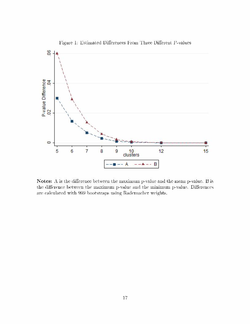
Figure 1: Estimated Di�erences From Three Di�erent P-values

Notes: A is the di�erence between the maximum p-value and the mean p-value. B isthe di�erence between the maximum p-value and the minimum p-value. Di�erencesare calculated with 999 bootstraps using Rademacher weights.

17

Table 1: Design of Monte Carlo SimulationsDesign Standard t-statistic Bootstrap

# Description Error distributed as Weights

1 OLS OLS N(0,1) -

2 Cluster ∼ N CRVE N(0,1) -

3 Cluster ∼ T CRVE T(G-1) -

4 Wild Cluster - Rademacher CRVE - Rademacher

5 Wild Cluster - Normal CRVE - ∼ N(0, 1)6 Wild Cluster - 6-point CRVE - 6-point equation (4)

7 Enumeration - Rademacher CRVE - Rademacher

Table 2: Results from Monte Carlo Study with Di�erent Numbers of ClustersNumber of Groups (G)

5 6 7 8 9 101 OLS ∼ N(0, 1) 0.471 0.478 0.483 0.485 0.488 0.4882 CRVE ∼ N(0, 1) 0.210 0.185 0.168 0.154 0.143 0.1343 CRVE ∼ T (G− 1) 0.097 0.098 0.096 0.094 0.092 0.0894 Wild 2pt Boot *0.037 *0.053 *0.056 *0.056 *0.055 *0.0545 Wild N(0, 1) Boot 0.072 0.070 0.072 0.072 0.071 0.0696 Wild 6pt Boot 0.070 0.067 0.063 0.061 0.057 0.0567 Enum. Lower Bound 0.118 0.095 0.084 0.068 0.062 0.0607 Enum. Upper Bound 0.000 0.059 0.067 0.061 0.058 0.058

Number of Groups (G)15 20 25 30

1 OLS ∼ N(0, 1) 0.489 0.495 0.490 0.4962 CRVE ∼ N(0, 1) 0.105 0.093 0.083 0.0813 CRVE ∼ t(G− 1) 0.080 0.075 0.069 0.0704 Wild 2pt Boot 0.050 0.050 0.047 0.0485 Wild N(0, 1) Boot 0.065 0.063 0.059 0.0596 Wild 6pt Boot 0.052 0.052 0.049 0.049

Notes: Rejection frequencies estimated with 50,000 replications and 399 bootstraps(Boot). * - estimate is not accurately calculated.

18

Table 3: Variable Means from Labour Force SurveyProvinces Provinces

without GRP with GRP

Pre Post Pre Post Sample

LFS

University Graduate 15.9% 20.2% 20.0% 22.7% 22-29

College Graduate 40.7% 39.0% 37.6% 35.0% 22-29

University or College Graduate 57.4% 59.5% 58.2% 58.1% 22-29

University or College Dropout 10.2% 10.0% 9.9% 10.4% 22-29

University Student 14.7% 15.7% 13.5% 14.7% 17-29

College Student 6.9% 7.8% 5.1% 5.6% 17-29

University or College Student 21.6% 23.5% 18.5% 20.3% 17-29

Sample: LFS data from years 2000-2013, ages 17-29, unless otherwise noted.

19

Table 4: Coe�cient Estimates and P-values from Various ProceduresAsymptotic p-values

OLS CRVE CRVE

coe� N(0, 1) N(0, 1) t(G− 1)University Graduate −11.229 0.002 0.000 0.028College Graduate −5.494 0.207 0.724 0.747University or College Graduate −15.708 0.000 0.231 0.317University or College Dropout 9.088 0.001 0.034 0.124University Student −0.188 0.935 0.973 0.975College Student 2.998 0.059 0.385 0.449University or College Student 2.810 0.284 0.596 0.633

Rademacher p-values

coe� boot enum�L enum�U

University Graduate −11.229 0.059 0.000 0.125College Graduate −5.494 0.677 0.625 0.750University or College Graduate −15.708 0.574 0.375 0.500University or College Dropout 9.088 0.441 0.375 0.500University Student −0.188 0.936 0.875 1.000College Student 2.998 0.532 0.375 0.500University or College Student 2.810 0.828 0.625 0.750

6-point p-values

coe� boot enum�L enum�U

University Graduate −11.229 0.039 0.042 0.043College Graduate −5.494 0.726 0.728 0.730University or College Graduate −15.708 0.524 0.523 0.525University or College Dropout 9.088 0.401 0.421 0.423University Student −0.188 0.980 0.971 0.972College Student 2.998 0.576 0.583 0.585University or College Student 2.810 0.726 0.719 0.721

20

A Proof of 2G−1 Unique Absolute Value t-statistics

Recall that a bootstrap sample is generated by:

y∗i = Xβ + u∗i , (7)

where u∗i is the Hadamard product u◦vi, and vi is the vector of draws of the bootstrapweights. The Rademacher weights are −1 and +1, so every possible vi is equal to

−1 ◦ vj for some i 6= j. These two bootstrap weight draws will generate the following

bootstrap samples: y∗i = Xβ+ u ◦ vi and y∗j = Xβ+ u ◦ vj. Since vj = −1 ◦ vi we canrewrite y∗j as y

∗j = Xβ − u ◦ vi.

We then test the null hypothesis β∗i , β∗j = βo and calculate t-statistics of the form:

(X ′X)−1X ′yi − βo(u′iui

X′X(n−k)

)1/2 . (8)

The denominator in equation (8) is constant for either i or j, as X and n − k are

invariant and u′iui = u′juj because uj = −1 ◦ ui.Let us consider the numerator in equation (8), where we have an expression in

terms of β∗i and βo. If we start with the expression:

(X ′X)−1X ′yi − βo,

using the identity that yi = Xβ + u ◦ vi we get the following,

(X ′X)−1X ′(Xβ + u ◦ vi)− βo.

With a little algebra we get:

(X ′X)−1X ′(Xβ + u ◦ vi)− βo=(X ′X)−1X ′Xβ + (X ′X)−1X ′(u ◦ vi)− βo=β − βo + (X ′X)−1X ′(u ◦ vi).

Because the bootstrap samples impose the null hypothesis, β = βo. The numerator

then simpli�es to:

(X ′X)−1X ′(u ◦ vi).

21

Since vi = −1 ◦ vj, the numerator for the t-statistic of β∗j will be the negative of

the numerator for the t-statistic of β∗i . The t-statistics are equal in absolute value,

because the denominators are also the same. If we reverse the sign on the weight

vector vi we reverse the sign of the t-statistic, but preserve the magnitude. Thus the

2G unique bootstrap samples will only result in 2G−1 unique t-statistics in absolute

value.

22