revista mexicana de vol. 11, no. 1 (2012) 177-192 ... · revista mexicana de ingeniería q uímica...

Revista Mexicana de Ingeniería Química

CONTENIDO

Volumen 8, número 3, 2009 / Volume 8, number 3, 2009

213 Derivation and application of the Stefan-Maxwell equations

(Desarrollo y aplicación de las ecuaciones de Stefan-Maxwell)

Stephen Whitaker

Biotecnología / Biotechnology

245 Modelado de la biodegradación en biorreactores de lodos de hidrocarburos totales del petróleo

intemperizados en suelos y sedimentos

(Biodegradation modeling of sludge bioreactors of total petroleum hydrocarbons weathering in soil

and sediments)

S.A. Medina-Moreno, S. Huerta-Ochoa, C.A. Lucho-Constantino, L. Aguilera-Vázquez, A. Jiménez-

González y M. Gutiérrez-Rojas

259 Crecimiento, sobrevivencia y adaptación de Bifidobacterium infantis a condiciones ácidas

(Growth, survival and adaptation of Bifidobacterium infantis to acidic conditions)

L. Mayorga-Reyes, P. Bustamante-Camilo, A. Gutiérrez-Nava, E. Barranco-Florido y A. Azaola-

Espinosa

265 Statistical approach to optimization of ethanol fermentation by Saccharomyces cerevisiae in the

presence of Valfor® zeolite NaA

(Optimización estadística de la fermentación etanólica de Saccharomyces cerevisiae en presencia de

zeolita Valfor® zeolite NaA)

G. Inei-Shizukawa, H. A. Velasco-Bedrán, G. F. Gutiérrez-López and H. Hernández-Sánchez

Ingeniería de procesos / Process engineering

271 Localización de una planta industrial: Revisión crítica y adecuación de los criterios empleados en

esta decisión

(Plant site selection: Critical review and adequation criteria used in this decision)

J.R. Medina, R.L. Romero y G.A. Pérez

Revista Mexicanade Ingenierıa Quımica

1

Academia Mexicana de Investigacion y Docencia en Ingenierıa Quımica, A.C.

Volumen 11, Numero 1, Abril 2012

ISSN 1665-2738

1Vol. 11, No. 1 (2012) 177-192

MODEL FOR THE DEVELOPMENT OF A LOW COST THERMAL MASS FLOWMETER

MODELO MATEMATICO PARA EL DESARROLLO DE UN MEDIDOR TERMICODE FLUJO MASICO DE BAJO COSTO

C. Garcıa-Arellano1∗ and O. Garcıa-Valladares2

1Posgrado en Ingenierıa, Energıa, Universidad Nacional Autonoma de Mexico (UNAM), Privada Xochicalco S/N,Temixco, 62580 Morelos, Mexico.

2Centro de Investigacion en Energıa (CIE), Universidad Nacional Autonoma de Mexico (UNAM), PrivadaXochicalco S/N, Temixco, 62580 Morelos, Mexico.

Received 05 of February 2009; Accepted 25 of September 2011

AbstractThis paper presents the mathematical model for the development of a water mass flow meter. Its operation principleis based on a relation between a constant input power (heat flow) provided to the system and the increase oftemperature in the test section. A numerical model of the thermal and fluid dynamic behavior of the thermal massflow meter is carried out; the governing equations (continuity, momentum and energy) inside the tube together withthe energy equation in the tube wall and insulation are solved iteratively in a segregated manner. The parametricstudy developed with the numerical model includes the tube diameter, tube length, and the power supply to thesystem, with the numerical results obtained and taking into account some restrictions on the system, the final designof the system has been obtained and constructed. A test procedure was carried out to show the technical feasibility ofthis system and an error of mass flow rate of ± 0.55 % was obtained. In relation to the cost, the errors of experimentalmeasurement are acceptable if they are compared with some of the more common available commercial systems withmuch higher cost.

Keywords: design, thermal mass flow meter, heat transfer, numerical model.

ResumenSe presenta el modelo matematico para el desarrollo de un medidor de flujo masico. Su principio de operacion estabasado en una relacion entre el flujo de calor suministrado a la seccion de prueba y la diferencia de temperaturasentre la entrada y la salida. Un modelo numerico del comportamiento termico y fluido-dinamico del medidortermico de flujo masico es desarrollado; las ecuaciones gobernantes dentro del tubo (continuidad, momentum yenergıa) junto con la ecuacion de la energıa en la pared del tubo y el aislante han sido resueltas iterativamente yde una forma segregada. El estudio parametrico desarrollado con el modelo numerico incluye el diametro, longituddel tubo ası como la potencia suministrada al sistema; con los resultados numericos obtenidos y tomando en cuentaalgunas restricciones sobre el sistema, el diseno final se obtuvo y se construyo. Se llevo a cabo un procedimiento depruebas para mostrar la factibilidad tecnica del sistema y se encontro un error en la medicion de flujo de ±0.55%. Enrelacion con el costo de construccion, los errores de las mediciones experimentales son aceptables si se comparancon algunos de los medidores comerciales mas comunmente usados de mayor precio.

Palabras clave: diseno, medidor termico de flujo masico, transferencia de calor, modelo numerico.

∗Corresponding author. E-mail: [email protected]. (52)(777)3250046 ext. 29746

Publicado por la Academia Mexicana de Investigacion y Docencia en Ingenierıa Quımica A.C. 177

Garcıa and Garcıa/ Revista Mexicana de Ingenierıa Quımica Vol. 11, No. 1 (2012) 177-192

1 IntroductionThe measurement and control of mass flow rateis critical in many industrial and experimentalapplications. Flux is defined as: the amount of massflow through an area per unit time. Currently thereare a wide variety of commercial flow meters, whichcan be constructed and designed for different operatingconditions. Its classification is based on their operationprinciple, as shown in (Table 1). Particularly, the costis an important factor to be considered in instrumentselection.

There are two methods to measure flow: direct andindirect. The second method was applied frequentlyby a simultaneous combination of volumetric flowand density meters, both depend on pressure andtemperature. Nevertheless, this is not accuratesince errors exist in the measurement instruments.Therefore, direct measurement methods are preferablein industrial processes (Zhang et al., 2006). Thermalmass flow meters are widely used in industry in orderto measure small flows.

Two techniques are commonly employed: thefirst is to provide a constant input power to asection of tubing and measure the temperature of thetube on both sides of the heated section, the flowskews the temperature distribution of the tube suchthat the downstream temperature is larger than theupstream value. This measured difference is linearlydependent upon mass flow rate. The second technique,heats the tube by maintaining a constant temperatureindependent of flow, in this way the amount of powerrequired to maintain the constant tube temperature isthen proportional to the mass flow rate in the tube. Forthis work the first technique is used.

To understand the operation principle of thermalmass flow meters, the term heat capacity must beconsidered; this is defined as the quantity of heatrequired to raise the temperature a specific numbers ofdegrees. In previous years several evaluations of thistype of systems have been developed. For example,experimental results for thermal mass flow metersworking under different conditions and using differenttypes of heaters arrangements have been reported by(Hawk and Baker, 1968; Komiya et al., 1988; Hinkleand Mariano, 1991; Tison, 1996; Toda et al., 1998;Rudent et al., 1998; Kim and Jang, 2001; Viswanathanet al., 2002; Viswanathan et al., 2002; Kim et al.,2007; Han et al., 2005); some authors have developednumerical models of the system in order to representthe phenomenology of it, for example: (Kim and Jang,2001; Kim et al., 2007; and Han et al., 2005).

The objective of this work is to present thedevelopment of a water mass Flow Meter (FM) oflow cost. For this purpose, a numerical simulationmodel of the thermal and fluid dynamic behavior ofthe thermal mass flow meter has been carried out.

In this paper, the operating principle will beexplained first; then the numerical model andnumerical algorithm are explained and a numericalparametric study has been carried out in order todesign the system; finally, the experimental set up andcomparisons of numerical solution and polynomialfunction (developed in order to obtain the mass flowrate) with experimental data are shown.

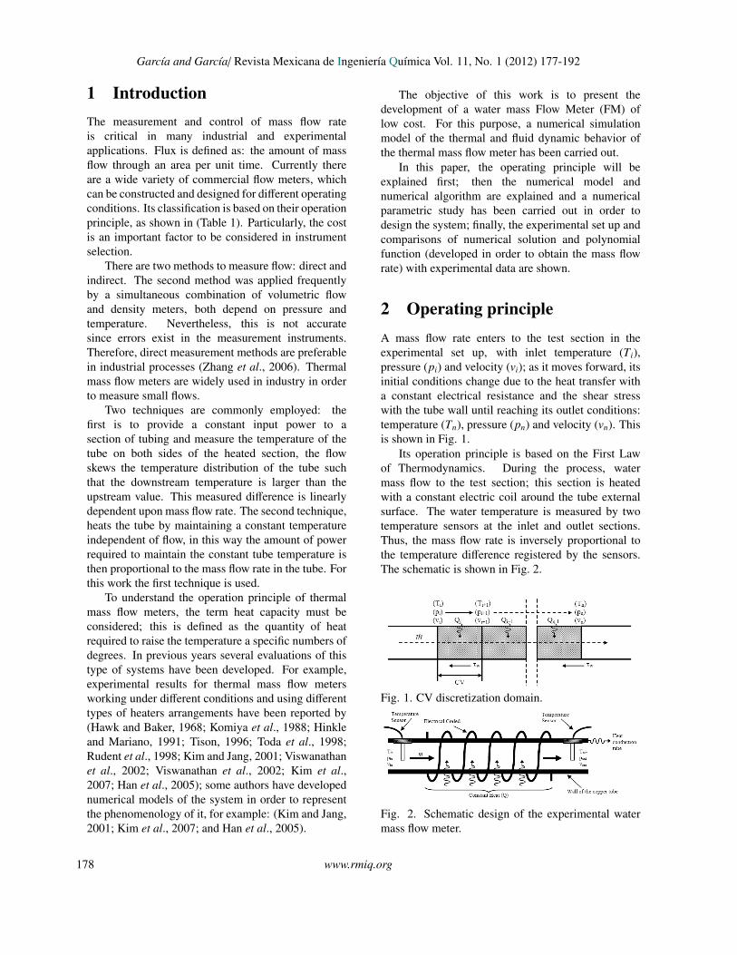
2 Operating principleA mass flow rate enters to the test section in theexperimental set up, with inlet temperature (Ti),pressure (pi) and velocity (vi); as it moves forward, itsinitial conditions change due to the heat transfer witha constant electrical resistance and the shear stresswith the tube wall until reaching its outlet conditions:temperature (Tn), pressure (pn) and velocity (vn). Thisis shown in Fig. 1.

Its operation principle is based on the First Lawof Thermodynamics. During the process, watermass flow to the test section; this section is heatedwith a constant electric coil around the tube externalsurface. The water temperature is measured by twotemperature sensors at the inlet and outlet sections.Thus, the mass flow rate is inversely proportional tothe temperature difference registered by the sensors.The schematic is shown in Fig. 2.

1

Fig. 1. CV discretization domain.

Fig. 2. Schematic design of the experimental water mass flow meter.


1


Fig. 2. Schematic design of the experimental water mass flow meter.

Fig. 2. Schematic design of the experimental watermass flow meter.

178 www.rmiq.org


Table 1. Flow meters classification (www.omega.com/techref.html)

Flow meter element Recommended service Typical accuracy % Cost

Orifice Clean, dirty liquids; ±2 to ±4% of full scale Lowsome slurries

Wedge Slurries and viscous ±0.5 to ±2% of full scale Highliquids

Venturi tube Clean, dirty and viscous ±1% of full scale Mediumliquids; some slurries

Flow nozzle Clean and dirty liquids ±1 to ±2% of full scale MediumPitot tube Clean liquids ±3 to ±5% of full scale LowElbow meter Clean, dirty liquids; ±5 to ±10% of full scale Low

some slurriesTarget meter Clean, dirty viscous ±1 to ±5% of full scale Medium

liquids; some slurriesVariable area Clean, dirty viscous ±1 to ±10% of full scale Low

liquidsPositive Clean, viscous liquids ±0.5% of flow rate MediumDisplacementTurbine Clean, viscous liquids ±0.25% of flow rate HighVortex Clean, dirty liquids ±1% of flow rate HighElectromagnetic Clean, dirty viscous ±0.5% of flow rate High

conductive liquids and slurriesUltrasonic (Doppler) Dirty, viscous liquids and ±5% of full scale High

slurriesUltrasonic Clean, viscous liquids ±1 to ±5% of full scale HighMass (Coriolis) Clean, dirty viscous liquids;

some slurries±0.1% of flow rate High

Mass (Thermal) Clean, dirty viscous liquids;some slurries

±1% of full scale High

Weir (V-notch) Clean, dirty liquids ±2 to ±5% of full scale MediumFlume (Parshall) Clean, dirty liquids ±2 to ±5% of full scale Medium

1

A continuación se enlistan las correcciones encontradas al archivo PDF pruebas de galera: Página 1 línea 37: eliminar palabra “aunque”. Página 2 línea 69: modificar , this way the amount of power por , in this way the amount of power Página 3 Fig. 3. Eliminar Fig. 3 y sustituirla por la siguiente figura:

a) Fluid flow inside the tube b) Tube wall c) Insulation d) Electrical coil between tube wall and insulation

Fig. 3. Node distribution along the thermal mass flow meter.

Página 4 línea 150: modificar r=(D4-D3)/2 for j=1 and r=(D5-D4)/(2(nr-1)) por r=(D2-D1)/2 for j=1 and r=(D3-D2)/(2(nr-1)) Página 5 línea 201: modificar following to obtain most of the results here presented (eliminar most of) Página 5 línea 226: sustituir en las 2 veces que aparece la variable ϕ por la variable φ Página 5 línea 253: modificar REPFPROP por REFPROP Página 5 línea 267: quitar un espacio entre Tin. _ From temperature Página 6 línea 316: sustituir flow por flow, (agregar una coma) Página 6 líneas 337, 338 y 339: eliminar el siguiente párrafo “Equation 10 can also be applied over the annular CVs in the insulation (see Fig. 3).” Página 7 línea 402: sustituir domain; por domain. Página 9 línea 493: sustituir 1.75 /m por 1.75 /m Página 9 línea 542: sustituir completely por fully Página 9 línea 566: acomodar número de la ecuación (14) como en el caso de la ecuación (13)

Fig. 3. Node distribution along the thermal mass flow meter.

www.rmiq.org 179


2

a) Fluid flow inside the internal tube b) External tube wall c) Internal tube wall d) Insulation e) Fluid flow inside the annulus (parallel or counter

flow) f) Electrical coil between external tube wall and

insulation Fig. 3. Node distribution along the thermal mass flow meter.

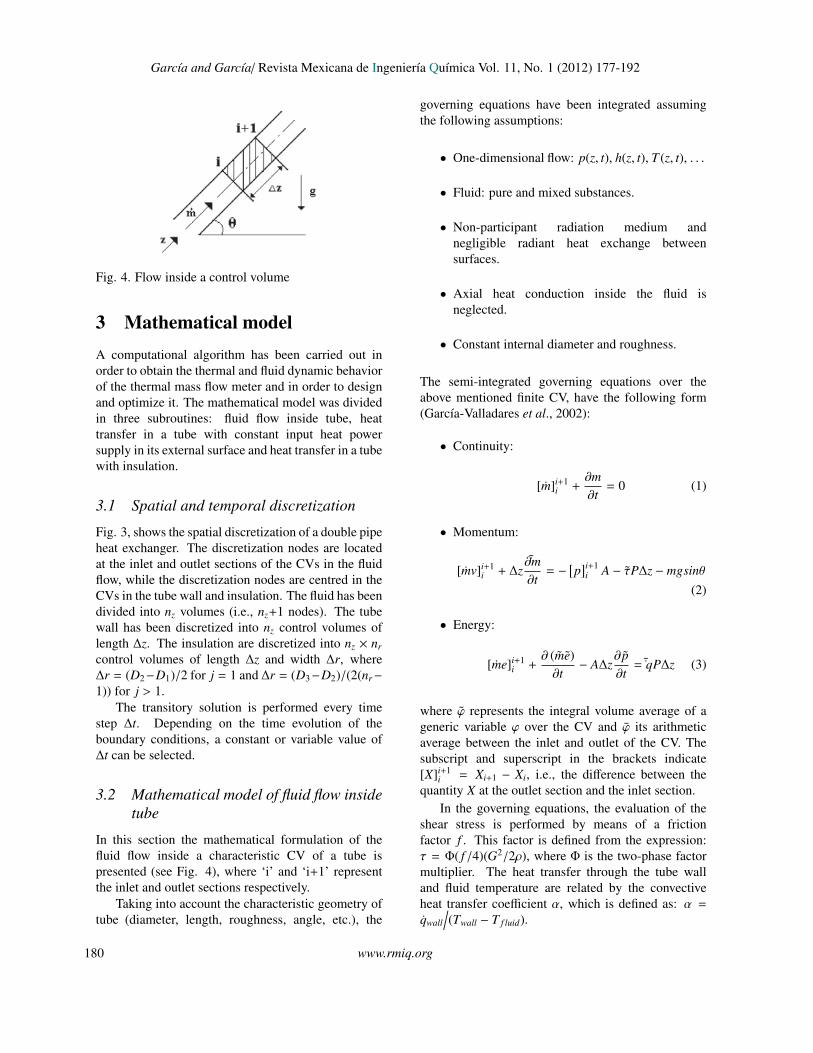
Fig. 4. Flow inside a control volume

Fig. 4. Flow inside a control volume

3 Mathematical modelA computational algorithm has been carried out inorder to obtain the thermal and fluid dynamic behaviorof the thermal mass flow meter and in order to designand optimize it. The mathematical model was dividedin three subroutines: fluid flow inside tube, heattransfer in a tube with constant input heat powersupply in its external surface and heat transfer in a tubewith insulation.

3.1 Spatial and temporal discretization

Fig. 3, shows the spatial discretization of a double pipeheat exchanger. The discretization nodes are locatedat the inlet and outlet sections of the CVs in the fluidflow, while the discretization nodes are centred in theCVs in the tube wall and insulation. The fluid has beendivided into nz volumes (i.e., nz+1 nodes). The tubewall has been discretized into nz control volumes oflength ∆z. The insulation are discretized into nz × nr

control volumes of length ∆z and width ∆r, where∆r = (D2−D1)/2 for j = 1 and ∆r = (D3−D2)/(2(nr−

1)) for j > 1.The transitory solution is performed every time

step ∆t. Depending on the time evolution of theboundary conditions, a constant or variable value of∆t can be selected.

3.2 Mathematical model of fluid flow insidetube

In this section the mathematical formulation of thefluid flow inside a characteristic CV of a tube ispresented (see Fig. 4), where ‘i’ and ‘i+1’ representthe inlet and outlet sections respectively.

Taking into account the characteristic geometry oftube (diameter, length, roughness, angle, etc.), the

governing equations have been integrated assumingthe following assumptions:

• One-dimensional flow: p(z, t), h(z, t), T (z, t), . . .

• Fluid: pure and mixed substances.

• Non-participant radiation medium andnegligible radiant heat exchange betweensurfaces.

• Axial heat conduction inside the fluid isneglected.

• Constant internal diameter and roughness.

The semi-integrated governing equations over theabove mentioned finite CV, have the following form(Garcıa-Valladares et al., 2002):

• Continuity:

[m]i+1i +

∂m∂t

= 0 (1)

• Momentum:

[mv]i+1i + ∆z

∂m∂t

= −[p]i+1i A − τP∆z − mgsinθ

(2)

• Energy:

[me]i+1i +

∂ (me)∂t

− A∆z∂p∂t

= ˜qP∆z (3)

where ϕ represents the integral volume average of ageneric variable ϕ over the CV and ϕ its arithmeticaverage between the inlet and outlet of the CV. Thesubscript and superscript in the brackets indicate[X]i+1

i = Xi+1 − Xi, i.e., the difference between thequantity X at the outlet section and the inlet section.

In the governing equations, the evaluation of theshear stress is performed by means of a frictionfactor f . This factor is defined from the expression:τ = Φ( f /4)(G2/2ρ), where Φ is the two-phase factormultiplier. The heat transfer through the tube walland fluid temperature are related by the convectiveheat transfer coefficient α, which is defined as: α =

qwall

/(Twall − T f luid).

180 www.rmiq.org


3.2.1 Evaluation of empirical coefficients

The mathematical model requires local informationabout friction factor f and the convective heat transfercoefficient α. This information is generally obtainedfrom empirical or semi-empirical correlations. Aftercomparing different empirical correlations presentedin the technical literature, we have selected thefollowing to obtain the results here presented: theconvective heat transfer coefficient is calculated usingthe Nusselt and the Gnieliski equations (Gnielinski,1976), for laminar and turbulent regimes respectively;and the friction factor is evaluated from theexpressions proposed by Churchill (1977).

3.2.2 Discretization equations of flow inside tubes

The discretized equations have been coupled usinga fully implicit step by step method in the flowdirection. From the known values at the inlet sectionand guessed values of the wall boundary conditions,the variable values at the outlet of each CV areiteratively obtained from the discretized governingequations. This solution (outlet values) is the inletvalues for the next CV. The procedure is carried outuntil the end of the tube is reached.

For each CV, a set of equations is obtained by adiscretization of the governing equations (1)-(3). Inthe section mathematical formulation, the governingequations have been directly presented on the basisof the spatial integration over finite CVs. Thus, onlytheir temporal integration is required. The transientterms of the governing equations are discretized usingthe following approximation: ∂ϕ/∂T (ϕ − ϕo)/∆t,where ϕ represents a generic dependent variable (ϕ =

h, p,T, ρ, ...); superscript “o” indicates the value of theprevious instant.

The averages of the different variables have beenestimated by the arithmetic mean between their valuesat the inlet and outlet sections, that is: ϕi ϕi ≡

(ϕi + ϕi+1)/2.Based on the numerical approaches indicated

above, the governing equations (1)-(3) can bediscretized to obtain the value of the dependentvariables (mass flow rate, pressure and enthalpy) atthe outlet section of each CV. The final form of thegoverning equations is given below.

The mass flow rate is obtained from the discretizedcontinuity equation,

mi+1 = mi −A∆z∆t

(ρ − ρo) (4)

The discretized momentum equation is solved forthe outlet pressure,

pi+1 = pi−∆zA

Φ f4

¯m2

2ρA2 P + ρAgsinθ +¯m − ¯mo

∆t+

[mv]i+1i

∆z

(5)

From the energy equation (3) and the continuityequation (1), the following equation is obtained for theoutlet enthalpy:

hi+1 =2qwall − ami+1 + bmi + cA∆z/∆t

mi+1 + mi + ρoAz/∆t(6)

wherea = v2

i+1 + gsinθ∆z − hi

b = v2i − gsinθ∆z + hi

c = 2(pi − po

i)− ρo

(hi − 2ho

i

)−

(ρv2

i − ρovo2

i

)Temperature and thermophysical properties are

evaluated using matrix functions of the pressure andenthalpy, refilled with the refrigerants propertiesevaluated using the REFPROP v.8.0 program(REFPROP, 2007):

T = f (p, h); ρ = f (p, h); ... (7)

The above mentioned conservation equations ofmass, momentum and energy together with thethermophysical properties, are applicable to transientflow. Situations of steady flow are particular casesof this formulation. Moreover, the mathematicalformulation in terms of enthalpy gives generality ofthe analysis (only one equation is needed for all theregions) and allows dealing with cases of mixtures offluids.

3.2.3 Boundary conditions

• Inlet conditions: the boundary conditions forsolving a step by step method directly arethe inlet mass flux min, pressure pin andtemperature Tin. From temperature and thepressure, enthalpy (our dependent variable) isobtained. Other boundary conditions such as(pin, pout) or (Tin,Tout) can be solved usinga Newton-Raphson algorithm. The methodis based on an iterative process where theinlet mass flow rate is updated until globalconvergence is reached.

• Solid boundaries: The wall temperature profilein the tube must be given. These boundary

www.rmiq.org 181


conditions are expressed in the energy equationin this form:

qwall = α(Twall − T f luid) (8)

3.2.4 Solver

In each CV, the values of the flow variables at theoutlet section of each CV are obtained by solvingiteratively the resulting set of algebraic equations(continuity, momentum, energy and state equationsmentioned above) from the known values at theinlet section and the boundary conditions. Thesolution procedure is carried out in this manner,moving forward step by step in the flow direction.At each cross section, the shear stresses andthe convective heat fluxes are evaluated using theempirical correlations obtained from the availableliterature (see Evaluation of Empirical Coefficients).The transitory solution is iteratively performed at eachtime step. If a transient case is analyzed, dependingon the time evolution of the boundary conditions, aconstant or variable value of ∆t can be selected.

Convergence is verified at each CV using thefollowing condition:(

1 −

∣∣∣∣∣∣ϕ∗i+1 − ϕi

∆ϕ

∣∣∣∣∣∣)< δ (9)

where ϕ refers to the dependent variables of mass flowrate, pressure and enthalpy; and ϕ∗ represents theirvalues at the previous iteration. The reference value∆ϕ is locally evaluated as ϕi+1 − ϕi. When this valuetends to be zero, ∆ϕ is substituted by ϕi.

3.3 Mathematical model of a tube withconstant input heat power supply in itsexternal surface

The conduction equation has been written assumingthe following hypotheses: one-dimensional transienttemperature distribution and negligible heatexchanged by radiation. A characteristic CV is shownin Fig. 5, where ’P’ represents the central node, ’E’and ’W’ indicate its neighbours. The CV-faces areindicated by ’e, ’w’, ’n’ and ’s’.

Integrating the energy equation over this CV, thefollowing equation is obtained:(

˜qsPs − ˜qnPn

)∆z +

(˜qw −

˜qe

)A = m

∂h∂t

(10)

where ˜qs is evaluated using the respective convectiveheat transfer coefficient and temperature of the fluid

flow, ˜qn is the constant heat power supply by electricalresistance, and the conductive heat fluxes are evaluatedfrom the Fourier law, that is: ˜qe = −λe(∂T /∂z)e and˜qw = −λw(∂T /∂z)w.

The following equation has been obtained for eachnode of the grid:

aiTwall,i = biTwall,i+1 + ciTwall,i−1 + di (11)

where the coefficients are,

ai =λwA∆z

+λeA∆z

+ αsPs∆z +A∆z∆t

ρcp bi = λeA∆z

ci =λwA∆z

di = (αsPsTs + ˜qnPn)∆z + A∆z∆t ρcpT o

wall,i

The coefficients mentioned above are applicable for2 ≤ i ≤ nz − 1; for i=1 and i = nz adequate coefficientsare used to take into account the axial heat conductionor temperature boundary conditions. The set of heatconduction discretized equations is solved using thealgorithm TDMA (Patankar, 1980).

3.4 Mathematical model of a tube withinsulation

The tube wall is solved in a similar way as describedin the previous section for the internal tube. Theconduction equation for the insulation has beenwritten assuming transient axisymmetric temperaturedistribution and negligible heat exchanged byradiation with the external ambient. The northand south interfaces are evaluated from the Fourierlaw, except in the tube-insulation interface (wherea harmonic mean thermal conductivity is used) andin the insulation-ambient interface (where the heattransfer by natural convection is introduced).

The following equation has been obtained for eachnode of the grid:

aPTwall,i, j =aETwall,i+1, j + aWTwall,i−1, j + aNTwall,i, j+1

+ aS Twall,i, j−1 + dP (12)

where the coefficients are,

aW =λwA∆z ; aE = λeA

∆z ; aN = λnPn∆z∆r ; aS =

λsPs∆z∆r ;

d′P =A∆z∆t

ρcP; aP = aW + aE + aN + aS + d′P;

dP = d′PT owall,i, j

The coefficients mentioned above are applicable for2 ≤ i ≤ nz − 1 and 2 ≤ j ≤ nr − 1; for the nodes inthe extremes (see Fig. 3) the following considerationshave been applied:

182 www.rmiq.org


3

Fig. 5. Heat fluxes in a CV of a solid element.

210

270

330

390

450

0

0.1

0.2

0.3

0.4

Tin

let-

outle

t (°C

)

Tube length (m)

Q heat flux (W)

0.25

0.5

0.75

Fig. 6. Increment of the water temperature in function of the tube length and heat power supply for

the ½” tube nominal diameter.


• For j = 1 forced convection is considered in thesouth face, tube thermal conductivity in east andwest faces and insulation thermal conductivityin north face, all these evaluated to the meantemperature between the nodes that separatedthem.

• For j = nr natural convection with theambient is considered [using the correlationdeveloped by Raithby and Hollands (Raithbyand Hollands, 1975) and also the conductionthrough the insulation external part of thickequal to ∆r/2, with thermal conductivityevaluated to the node temperature.

• For i = 1 and i = nz adequate coefficientsare used to take into account the axial heatconduction or temperature boundary conditions.

4 Numerical algorithm

The solution process is carried out on the basis of aglobal algorithm that solves in a segregated mannerthe fluid flow inside tube, heat transfer in a tubewith constant input heat power supply in its externalsurface and heat transfer in a tube with insulation. Thecoupling between the three main subroutines has beenperformed iteratively following the procedure:

• For fluid flow inside tube, the equations aresolved considering the tube wall temperaturedistribution as boundary condition, andevaluating the convective heat transfer and fluidtemperature in each CV.

• For heat transfer in a tube with constantheat power supply in its external surface,the temperature distribution in the tube is re-calculated using the fluid flow temperatureand the convective heat transfer coefficientsevaluated in the preceding steps and consideringthe constant input heat power supply by theelectric resistance and the ambient thermallosses calculated in the next step.

• For heat transfer in a tube with insulation,the ambient thermal losses are calculatedconsidering the tube wall temperaturedistribution calculated in the preceding stepand the insulation thickness and the naturalconvective heat transfer coefficients evaluatedin the external ambient.

The global convergence is reached when between twoconsecutive loops of the three main subroutines a strictconvergence criterion is verified for all the CVs in thedomain.

The mass flow rate through the systems issolved using a Newton-Raphson algorithm with thefollowing boundary condition (Tin,Tout) registered bythe thermocouples in the experimental set up. Themethod is based on an iterative process where the inletmass flow rate is updated until global convergence isreached.

Based on the above mentioned mathematicalmodel and numerical algorithm, a code has beendeveloped for the detail numerical simulation of thethermal and fluid dynamic behavior of the thermalmass flow meter. The numerical results obtained bythe mathematical model for this particular mass flowmeter are presented in the design and optimization andthe experimental validation sections. All numericalresults obtained are grid independence solutions.

The numerical model developed is based on theapplications of governing equations and used generalempirical correlations (any correction factor has beenused); for this reason, it is possible to make use of itto other fluids, mixtures and operating conditions; itallows using the model developed as an important toolto design these kinds of systems.

5 Design of the thermal mass flowmeter

Based on the mathematical model of the thermal andfluid dynamic behavior of the thermal mass flow metercarried out, the design of this system is described inthis section.

The main objective is to obtain a water mass flowmeter of low cost with a good performance for theuser (i.e. reasonable mass flow rate error, low pressuredrop, reasonable consume of energy, etc.). In orderto reach this objective, the numerical model has beenused in order to obtain a parametric study of thissystem.

The following restrictions have been considered

www.rmiq.org 183


in order to design and optimize the system: a) therange of the mass flow rate was fixed from 3 to 17kg/min; b) the Reynolds number over the entire rangeof mass flow rate must be in the turbulent region(higher than 5000 in order to be sure that the systemis not working in the laminar or transition regionwere the heat transfer coefficients decrease significantand it can affect the system performance); c) dueto the temperature sensors used in the system havean accuracy of ±0.2 oC, the minimum difference oftemperature between the inlet and outlet section is0.2 oC; d) material of the tube with high thermalconductivity; e) low pressure drop in the systemis required in order to not perturb significantly theprocess where the system can be install.

The parametric study developed includes the tubediameter, tube length, and the power supply to thesystem shown in (Table 2). For all the cases, thenumerical model has fixed the following parameters:inlet water temperature (25 oC), ambient temperature(30 oC), thickness of flexible foam insulation ( 3

4 ”,19.05 mm) for all the tube diameters and copper tube(due to its high thermal conductivity).

The average Reynolds numbers obtained by the

numerical model for the different tube diameterconsidering the lowest mass flow rate (3 kg/min) are:8939 (for 1

4 ”), 5167 (for 12 ”) and 3587 (for 3

4 ”); thepressure drop obtained for highest mass flow rate (17kg/min) and the highest length (0.75 m) was: 31.6 kPa,2.3 kPa and 0.4 kPa respectively or 8.95 W, 0.65 Wand 0.11 W of power consumption (assuming that thepower consumption is approximately equal to pressuredrop multiplied by the mass flow rate and divided bythe fluid density). According to these results and therestrictions mentioned above, the 1

4 ” nominal diametertube has been discarded due to the high pressuredrop obtained and the 3

4 ” nominal diameter has beendiscarded due to the small Reynolds number obtainedthat can produce that the system can operate in thetransition zone between laminar and turbulent flow.

Fig. 6 shows the increment of the watertemperature in function of the tube length and heatpower supply for the 1

2 ” tube nominal diameter.According to the restriction of minimum temperaturedifference between the inlet and outlet section of 0.2oCthe heat powers of 210 and 270 W has been eliminatedand due to save energy in the system operation the 330W heat power supply has been selected.

Table 2. Parametrical study

Variable Range

Tube diameter (copper commercial tubes) 14 ”, 1

2 ”, 34 ” (nominal diameters)

(Internal, external) diameters (8,9.52), (13.84,15.87), (19.94,22.23) mmTube length 0.25, 0.50, 0.75 mHeat power 210, 270, 330, 390, 450 W

3


210

270

330

390

450

0

0.1

0.2

0.3

0.4

Tin

let-

outle

t (°C

)

Tube length (m)

Q heat flux (W)

0.25

0.5

0.75

Fig. 6. Increment of the water temperature in function of the tube length and heat power supply for

the ½” tube nominal diameter.

Fig. 6. Increment of the water temperature in function of the tube length and heat power supply for the 12 ” tube

nominal diameter.

184 www.rmiq.org


Due to the electrical resistance foundcommercially has a resistance of 1.75 Ω/m with adiameter of 5 mm, the length necessary to reach 330W of heat power is 3.08 m (considering the electricalenergy supply in Mexico of 127 V a.c. and in order tonot used voltage regulators); this length is impossibleto be coiled in the 0.25 m length tube and the 0.75m length tube has been discarded in order to obtain asystem that can be mounted in an easy way (reducingspace) in experimental systems.

The final design obtained for the thermal massflow meter by the numerical analysis has the followingcharacteristics: 1

2 ” nominal diameter of copper tube,0.5 m length, 330 W of heat power and a thickness ofthe flexible foam insulation of 3

4 ”.With the numerical model and the final geometry

conditions given above, the following polynomialequation has been developed in order to calculatetheoretically the mass flow rate of the system infunction of the temperature difference between theinlet and outlet section and the power supply by theelectrical coiled:

mwater = 0.14618 · Q · [ - 0.846 · ∆T5inlet - outlet

+4.173 · ∆T4inlet - outlet - 8.068 · ∆T3

inlet - outlet

+7.796 · ∆T2inlet - outlet - 3.959 · ∆Tinlet - outlet

+ 1.0] (kg/min)

(13)

6 Experimental setup

Based on the numerical model the final design ofthe thermal mass flow meter mentioned above wasobtained and constructed. A domestic Mexicanvoltage is used to obtain this power supply withoutusing voltage regulators.

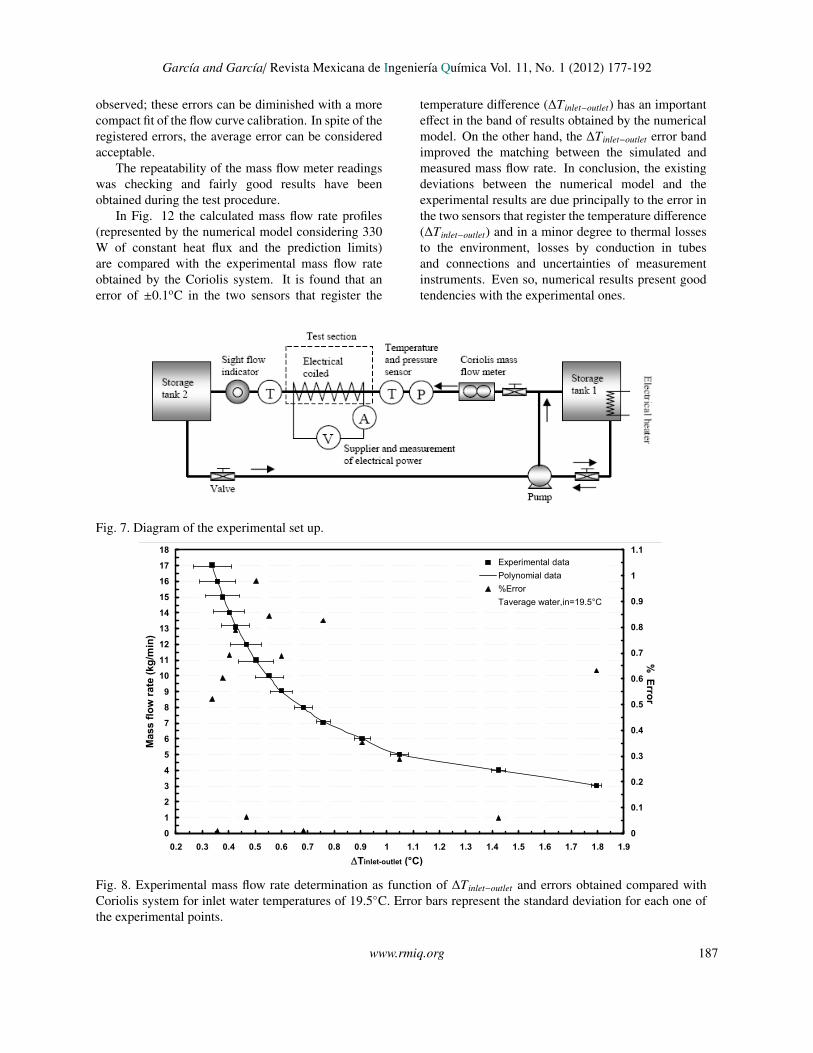
Fig. 7 shows a general diagram of the experimentalset up. The electrical power supplier is a flexibleelectrical resistance of 3.08 m with a diameter of5 mm coiled over the external tube wall in orderto maintain a constant heat flux; two sensors oftemperature (thermistors with an accuracy of ±0.2C)were installed at the inlet and outlet sections.

A Coriolis equipment with an accuracy of ±0.1%(Coriolis, Endress Hausser Instruction Manual, 2000)of mass flow rate was installed on the work line inorder to determine the water mass flow rate acrossthe test section; this error is taken into account in theexperimental measurements; but the error is too smallto affect significantly the experimental results.

At the end of the test section a sight flow indicatorwas installed in order to visualize the flow behavior.Table 3 presents the characteristics of the experimentalthermal mass flow meter developed.

All experimental data are registered with anacquisition data logger. Computer software wasdeveloped and tested in order to register, analyze andprocess all the involved variables.

The minimum distance to have a fully developedflow and obtain reliable results is 12 diametersto the entrance and 10 diameters at outlet section(for the system developed 0.152 m and 0.127 mrespectively). This distance was taken into accountin the experimental set up. Major obstructions suchthrottled valves, elbows or pumps will require longerstraight runs.

Table 3. Developed mass flow meter characteristics

Fluid WaterMass flow rate 3-17 kg/minOperation temperature 15C - 60CEnergy supply 127 V a.c.Heat power supply 330 WDimensions 0.5 m length, 1

2 ”Ø nominal (coppertube)

∆Tinlet−outlet minimum 0.2 CFlexible foam insulation 0.5 m length, 1

2 ” Ø ,34 ” thickness

7 Test procedure

The objective of this test procedure is to determineexperimentally the mass flow rate across the sectiontest and its percentage of error with respect to aCoriolis mass flow meter. The characteristics totake into account include (Belforte et al., 1997):type of fluid (liquid or gas), physical propertiesto be measured, working conditions, accuracy andprecision.

Three characteristics polynomials wereexperimentally obtained for each one of thewater inlet temperatures tested by means of thetemperature difference registered by the inlet andoutlet temperature sensors and the mass flow metermeasured by the Coriolis instrument.

www.rmiq.org 185


For inlet water temperature of 20o C

mwater = 51.983 - 177.78 · ∆Tinlet - outlet

+290.45 · ∆T2inlet - outlet - 243.73 · ∆T3

inlet - outlet

+100.43 · ∆T4inlet - outlet - 16.023 · ∆T5

inlet - outlet

(kg/min)

(14)



+288.17 · ∆T2inlet - outlet - 254.16 · ∆T3

inlet - outlet

+ 110.87 · ∆T4inlet - outlet - 18.876 · ∆T5

inlet - outlet

(kg/min)

(15)



−32.382 · ∆T2inlet - outlet + 106.5 · ∆T3

inlet - outlet

−82.282 · ∆T4inlet - outlet + 20.681 · ∆T5

inlet - outlet

(kg/min)

(16)

These five order polynomial equations have beenintegrated into the developed software to be validatedwith new experimental data in order to estimate therepeatability and error of this system. For intermediatewater inlet temperatures a linear interpolation of thesepolynomial equations is used.

7.1 Experimental validation

The experimental test begins with the water circulationfrom storage tank 1 to 2 (see Fig. 7). Previously,inlet water temperature has been fixed by an electricalheat supplier installed inside the storage tank 1. Thewater flow enters into the section test, where a constantheat flux is applied through all the external surfaceof the tube wall, two sensors register the temperaturedifference (∆Tinlet−outlet) that is used in the polynomialequation according to each case.

Experimental values were registered each 5 s;twenty tests were performed for each temperaturein order to verify the accuracy and error of thissystem. Mass flow rate test validation begins with3 kg/min and it is increased in 1 kg/min until reach17 kg/min. The steady state condition for eachone of the experimental points is reached once the(∆Tinlet−outlet) is maintained constant in ±0.2C; forlow flows (3-8 kg/min) the stabilization time requiredis approximately 30 s, meanwhile for high flows(9-17 kg/min) the stabilization time is reduced toapproximately 15 s.

With flows higher than 18 kg/min, themeasurement errors (∆Tinlet−outlet, minimum) are higherthan the difference temperature between inlet andoutlet temperature sensors, for this reason, the massflow range was limited until 17 kg/min in experimentaltests. In order to evaluate mass flow rate over 18kg/min a higher heat power had to be applied ora by-pass (that will be explained below) can beimplemented.

For the comparison with experimental data, thefollowing definitions are used:

%error = 100 ·

∣∣∣mreal − mpred

∣∣∣mreal

(17)

%average · error =1k

k∑i=1

%errori (18)

where k is the number of data points and mreal isthe measurement obtained by the Coriolis mass flowmeter.

Fig. 8 presents the experimental results for a testwith an inlet water temperature of 19.5 C; in this casean average error of ±0.46% and a maximum error of±0.98% of mass flow rate are observed with a standarddeviation of 0.04. In the experimental tests, the errorbars represent the standard deviation for each one ofthe measured points.

Fig. 9 presents the mass flow rate obtained bya linear interpolation for two polynomial equations(20 C and 40 C respectively) for the inlet watertemperature of 24.4 C. With this interpolation, massflow rates with a smaller degree of uncertainty canbe obtained. From this figure it can be seenthat the experimental flows registered by the linearinterpolation adjust fairly good to the mass flow rateregister by the Coriolis instrument. An average errorof ±0.46% is observed with a maximum error of±0.84% of mass flow rate and a standard deviation of0.034.

Fig. 10 shows the experimental mass flow rate testwith inlet water temperature of 40.4 C, an averageerror of ±0.31%, with a maximum error of ±0.83%and a standard deviation of 0.047 have been obtained.

For the case presented in Fig. 11, an inlet watertemperature of 60.1 C was used, an average error of±0.91%, a maximum error of ±1.91% of mass flowrate and a standard deviation of 0.06 are observed.Although the experimental results obtained in this casefrom the corresponding polynomial equation have agood agreement with the measured real mass flow rate,errors higher than the previous tests (figs. 8-10) can be

186 www.rmiq.org


observed; these errors can be diminished with a morecompact fit of the flow curve calibration. In spite of theregistered errors, the average error can be consideredacceptable.

The repeatability of the mass flow meter readingswas checking and fairly good results have beenobtained during the test procedure.

In Fig. 12 the calculated mass flow rate profiles(represented by the numerical model considering 330W of constant heat flux and the prediction limits)are compared with the experimental mass flow rateobtained by the Coriolis system. It is found that anerror of ±0.1oC in the two sensors that register the

temperature difference (∆Tinlet−outlet) has an importanteffect in the band of results obtained by the numericalmodel. On the other hand, the ∆Tinlet−outlet error bandimproved the matching between the simulated andmeasured mass flow rate. In conclusion, the existingdeviations between the numerical model and theexperimental results are due principally to the error inthe two sensors that register the temperature difference(∆Tinlet−outlet) and in a minor degree to thermal lossesto the environment, losses by conduction in tubesand connections and uncertainties of measurementinstruments. Even so, numerical results present goodtendencies with the experimental ones.

4

Fig. 7. Diagram of the experimental set up.

0

1

2

3

4

5

6

7

8

9

10

11

12

13

14

15

16

17

18

0.2 0.3 0.4 0.5 0.6 0.7 0.8 0.9 1 1.1 1.2 1.3 1.4 1.5 1.6 1.7 1.8 1.9

Tinlet-outlet (°C)

Mas

s fl

ow

rat

e (k

g/m

in)

0

0.1

0.2

0.3

0.4

0.5

0.6

0.7

0.8

0.9

1

1.1Experimental data

Polynomial data

%Error

Taverage water,in=19.5°C

% E

rror

Fig. 8. Experimental mass flow rate determination as function of Tinlet-outlet and errors obtained

compared with Coriolis system for inlet water temperatures of 19.5°C. Error bars represent the standard deviation for each one of the experimental points.


4


0

1

2

3

4

5

6

7

8

9

10

11

12

13

14

15

16

17

18

0.2 0.3 0.4 0.5 0.6 0.7 0.8 0.9 1 1.1 1.2 1.3 1.4 1.5 1.6 1.7 1.8 1.9

Tinlet-outlet (°C)

Mas

s fl

ow

rat

e (k

g/m

in)

0

0.1

0.2

0.3

0.4

0.5

0.6

0.7

0.8

0.9

1

1.1Experimental data

Polynomial data

%Error


% E

rror



Fig. 8. Experimental mass flow rate determination as function of ∆Tinlet−outlet and errors obtained compared withCoriolis system for inlet water temperatures of 19.5C. Error bars represent the standard deviation for each one ofthe experimental points.

www.rmiq.org 187


The average error between the numerical modeland the experimental results is ±7.41% of massflow rate. The error is increases when ∆Tinlet−outlet

is reduced due to the temperature sensors accuracy±0.2oC.

5

0

1

2

3

4

5

6

7

8

9

10

11

12

13

14

15

16

17

18

0.2 0.3 0.4 0.5 0.6 0.7 0.8 0.9 1 1.1 1.2 1.3 1.4 1.5 1.6 1.7 1.8 1.9

Tinlet-outlet (°C)

Mas

s fl

ow

rat

e (k

g/m

in)

0

0.1

0.2

0.3

0.4

0.5

0.6

0.7

0.8

0.9

Experimental data

Polynomial data

%Error


% E

rror



0

1

2

3

4

5

6

7

8

9

10

11

12

13

14

15

16

17

18

0.2 0.3 0.4 0.5 0.6 0.7 0.8 0.9 1 1.1 1.2 1.3 1.4 1.5 1.6 1.7

Tinlet-outlet (°C)

Mas

s fl

ow

rat

e (k

g/m

in)

0

0.1

0.2

0.3

0.4

0.5

0.6

0.7

0.8

0.9

Experimental data

Polynomial data

%Error


% E

rror

Fig. 10. Experimental mass flow rate determination as function of Tinlet-outlet and errors

obtained compared with Coriolis system for inlet water temperatures of 40.4°C. Error bars represent the standard deviation for each one of the experimental points.


5

0

1

2

3

4

5

6

7

8

9

10

11

12

13

14

15

16

17

18

0.2 0.3 0.4 0.5 0.6 0.7 0.8 0.9 1 1.1 1.2 1.3 1.4 1.5 1.6 1.7 1.8 1.9

Tinlet-outlet (°C)

Mas

s fl

ow

rat

e (k

g/m

in)

0

0.1

0.2

0.3

0.4

0.5

0.6

0.7

0.8

0.9

Experimental data

Polynomial data

%Error


% E

rror



0

1

2

3

4

5

6

7

8

9

10

11

12

13

14

15

16

17

18

0.2 0.3 0.4 0.5 0.6 0.7 0.8 0.9 1 1.1 1.2 1.3 1.4 1.5 1.6 1.7

Tinlet-outlet (°C)

Mas

s fl

ow

rat

e (k

g/m

in)

0

0.1

0.2

0.3

0.4

0.5

0.6

0.7

0.8

0.9

Experimental data

Polynomial data

%Error


% E

rror




188 www.rmiq.org


6

0

1

2

3

4

5

6

7

8

9

10

11

12

13

14

15

16

17

18

0 0.1 0.2 0.3 0.4 0.5 0.6 0.7 0.8 0.9 1 1.1 1.2 1.3 1.4 1.5 1.6 1.7

Tinlet-outlet (°C)

Mas

s fl

ow

rat

e (k

g/m

in)

0

0.2

0.4

0.6

0.8

1

1.2

1.4

1.6

1.8

2

Experimental data

Polynomial data

%Error


% E

rror



0123456789

101112131415161718192021222324

0.2 0.3 0.4 0.5 0.6 0.7 0.8 0.9 1 1.1 1.2 1.3 1.4 1.5 1.6 1.7

Tinlet-outlet (°C)

Ma

ss f

low

rat

e (k

g/m

in)

Numerical model

Polynomial approximation 20°C



---- Numerical model considering ±0.1°C of error of the temperature sensors

Fig. 12. Comparison of numerical model vs. experimental mass flow rate obtained by Coriolis

system. The profile computed by the numerical model are denoted by solid lines; the predictions limits from the uncertainty analysis are represented by dashes lines.


6

0

1

2

3

4

5

6

7

8

9

10

11

12

13

14

15

16

17

18

0 0.1 0.2 0.3 0.4 0.5 0.6 0.7 0.8 0.9 1 1.1 1.2 1.3 1.4 1.5 1.6 1.7

Tinlet-outlet (°C)

Mas

s fl

ow

rat

e (k

g/m

in)

0

0.2

0.4

0.6

0.8

1

1.2

1.4

1.6

1.8

2

Experimental data

Polynomial data

%Error


% E

rror



0123456789

101112131415161718192021222324

0.2 0.3 0.4 0.5 0.6 0.7 0.8 0.9 1 1.1 1.2 1.3 1.4 1.5 1.6 1.7

Tinlet-outlet (°C)

Ma

ss f

low

rat

e (k

g/m

in)

Numerical model




---- Numerical model considering ±0.1°C of error of the temperature sensors

Fig. 12. Comparison of numerical model vs. experimental mass flow rate obtained by Coriolis

system. The profile computed by the numerical model are denoted by solid lines; the predictions limits from the uncertainty analysis are represented by dashes lines.

Fig. 12. Comparison of numerical model vs. experimental mass flow rate obtained by Coriolis system. The profilecomputed by the numerical model are denoted by solid lines; the predictions limits from the uncertainty analysis arerepresented by dashed lines.

www.rmiq.org 189


7

Fig. 13. Method to obtained higher mass flow rates with moderate input power supply by means of

a by-pass section Fig. 13. Method to obtained higher mass flow rates with moderate input power supply by means of a by-pass section.

The error is diminished when ∆Tinlet−outlet

increases; i.e. for the case of an interval higher than0.6C the error diminished to ±5.38%, and for aninterval higher than 1.0C the error is ±4.46%.

When the experimental results obtained by meansof the polynomial equations are compared to the realvalue measured by the Coriolis mass flow meter, anaverage error of ±0.55% is obtained; this error isacceptable considering the construction cost.

Experimentally, the measured mass flow rates canbe increased (to values higher than 17 kg/min) with thesame principle without increasing the input power, bymeans of a by-pass in the test section; thus, there isa proportional correspondence of the total mass flowrate measured in the experimental section, respect tothe mass flow rate that crosses the by-pass section (k),as shown in Fig. 13.

8 Accuracy and cost of theexperimental mass flow metercompared to commercial flowmeters

The simple design of the experimental thermal massflow meter developed produces a cheap systemwithout movable parts. The device can be a viableand competitive option in the market accordingto the working conditions and mass flow rate tobe used. In relation to the cost, the errors ofexperimental measurement are acceptable if theyare compared with some of the more commoncommercial systems; for example, a comparison of thedeveloped mass flow meter with an electromagneticor positive displacement mass flow meter available

in the market that have similar uncertainties in massflow rates measurement (±0.55%), shows that thesystem developed reduced the price between 10 and11 times. Thus, it is demonstrated that an elevatedinvestment is not necessary in order to obtain reliableresults. Moreover, the characteristic polynomialequation obtained can be implemented in an easy wayin a chip.

Concluding remarksAn experimental thermal mass flow meter of lowcost has been developed; its operation is based onthe solution of governing equation presented in thenumerical model section.

With the parametric study developed with thenumerical model and taking into account somerestrictions on the system, the final design of thesystem has been obtained and constructed.

The experimental mass flow meter has beendeveloped in a mass flow rate range from 3 to 17kg/min. Three polynomial equations at 20 oC, 40 oCand 60 C have been developed in order to characterizethe experimental mass flow meter, these equationsare based on the inlet-outlet temperatures registeredand the heat power supplied. The application of thepolynomial equations allowed obtaining directly themass flow rate across the test section. There was noneed of measuring other physical properties; thereforeno additional equipment was required. In addition,the developed flow meter has no movable parts so itwill not have mechanical failures and the polynomialequation can be implemented in an easy way in a chip.

The experimental average error obtained withthe developed system is ±0.55% of mass flow rate,this error is acceptable when construction cost and

190 www.rmiq.org


measure quality are compared.The numerical model developed is based on the

applications of governing equations and used generalempirical correlations (any correction factor has beenused); for this reason, it is possible to make use ofit to other fluids, mixtures and operating conditions(including gas or two-phase flow); it allows using themodel developed as an important tool to design thesekinds of systems.

AcknowledgementsThis work had been financed by CONACyT projectU44764-Y. The authors thank Dr. V.H. Gomez forthe technical support, Dr. Jorge Andaverde for thecontribution in the study of the experimental errorsand to CONACyT, Mexico, for the support providedfor the student scholarship 173571.

NomenclatureA cross section area, m2

cp specific heat at constant pressure, J kg−1 K−1

D tube diameter, me specific energy (h+v2/2+gzsin θ), J kg−1

f friction factorg acceleration due to gravity, m s−2

G mass velocity, kg m−2 s−1

h enthalpy, J kg−1

k number of data pointsL length, mm mass, kgm mass flow rate, kg s−1

n number of control volumesp pressure, PaP perimeter, mq heat flux per unit area, W m−2

Q heat flux, Wt time, sT temperature, Kv velocity, m s−1

z axial direction, mGreek lettersα heat transfer coefficient, W m−2 K−1

∆r radial discretization step, m∆t temporal discretization step, s∆T temperature difference, K∆z axial discretization step, mØ tube diameter, mΦ two-phase frictional multiplierθ angle, radλ thermal conductivity, W m−1 K−1

ρ density, kg m−3

τ shear stress, PaSubscripts

e easti inletn northpred predicteds southw west

Superscripts˜ integral average over a CV:

φ = (1/∆z)z+∆z∫zφdz

previous instant∗ previous iteration

ReferencesBelforte G., Carello M., Mazza L. and Pastorelli

S. (1997). Test bench for flow ratemeasurement: calibration of variable areameters. Measurement 20, 67-74.

Churchill S.W. (1977). Friction equation spans allfluid flow regimes. Chemical Engineering 84,91-92.

Coriolis, Endress Hausser Instruction Manual(2000).

Garcıa-Valladares O., Perez-Segarra C.D. and OlivaA. (2002). Numerical simulation of capillary-tube expansion devices behaviour with pureand mixed refrigerants considering metastableregion. Part I: Mathematical formulation andnumerical model. Applied Thermal Engineering22, 173-182.

Garcıa-Valladares O., Perez-Segarra C.D. and RigolaJ. (2004). Numerical simulation of double-pipe condensers and evaporators. InternationalJournal of Refrigeration 27, 656-670.

Gnielinski V. (1976). New equations for heat andmass transfer in turbulent pipe and channel flow.International Chemical Engineering 16, 359-368.

Han Y., Kim D. K. and Kim S. J. (2005). Study on thetransient characteristics of the sensor tube of athermal mass flow meter. International Journalof Heat and Mass Transfer 48, 2583-2592.

Hawk C. E. and Baker W. C. (1968). Measuringsmall gas flows into vacuum systems. The

www.rmiq.org 191


Journal of Vacuum Science and Technology 6,255-257.

Hinkle L. D. and Mariano C. F. (1991). Towardunderstanding the fundamental mechanisms andproperties of the thermal mass flow controller.The Journal of Vacuum Science and TechnologyA 9, 2043-2047.

Kim D. K., Han I. Y. and Kim S. J. (2007). Studyon the steady-state characteristics of the sensortube of a thermal mass flow meter. InternationalJournal of Heat and Mass Transfer 50, 1206-1211.

Kim S. J. and Jang S. P. (2001). Experimental andnumerical analysis of heat transfer phenomenain a sensor tube of a mass flow controller.International Journal of Heat and MassTransfer 44, 1711-1724.

Komiya K., Higuchi F. and Ohtani K. (1988).Characteristics of a Thermal Gas Flowmeter.Review of Scientific Instruments 59, 477-479.

Patankar S.V. (1980). Numerical Heat Transfer andFluid Flow. New York: McGraw-Hill.

Raithby G. D. and Holland G. T. (1975). Advances inHeat Transfer, ed. by Irvine and Hartnett, vol.11, Academic Press, New York.

REFPROP v8.0, Reference fluid thermodynamic andtransport properties. NIST Standard ReferenceData Program, USA, 2007.

Rudent P., Navratil P., Giani A. and Boyer A.(1998). Design of new sensor for mass flowcontroller using thin film technology based onan analytical thermal model. The Journal ofVacuum Science and Technology A 16, 3559-3563.

Tison S. A. (1996). A critical evaluation of thermalmass flow meters. The Journal of VacuumScience and Technology A 14, 2582-2591.

Toda K., Maeda Y., Sanemasa I., Ishikawa K. andKimura N. (1998). Characteristics of a thermalmass-flow sensor in vacuum systems. Sensorsand Actuators A 69, 62-67.

Viswanathan M., Rajesh R. and Kandaswamy A.(2002). Design and development of thermalmass flowmeters for high pressure applications.Flow Measurement and Instrumentation 13, 95-102.

Viswanathan M., Kandaswamy A., Sreekala S.K. and Sajna K. V. (2002). Development,modeling and certain investigations on thermalmass flow meters. Flow Measurement andInstrumentation 12, 353-360.

www.omega.com/techref.html

Zhang H., Huang Y. and Sun Z. (2006). A studyof mass flow rate measurement based on thevortex shedding principle. Flow Measurementand Instrumentation 17, 29-38.

192 www.rmiq.org

revista mexicana de vol. 11, no. 1 (2012) 177-192 ... · revista mexicana de ingeniería q uímica...

Documents