Revista Sergipana de Matematica e Educacao Matematica

https://doi.org/10.34179/revisem.v6i1.14809

REVISITING THE ARMS RACE RICHARDSON’S MODEL: BEYONDTHE TWO ACTORS’ APPROACH

Luıs MartinsUniversity of Brasılia

luismartinsxd@gmail.com

Resumo

O modelo de Richardson e classico no campo das Relacoes Internacionais, ao descrevera corrida armamentista entre dois atores, por meio de sistema de equacoes diferenci-ais ordinarias com coeficientes constantes acerca dos respectivos orcamentos militares.Neste artigo, estendemos o modelo de Richardson para abarcar um numero arbitrariode atores e investigar se existem fatores de escala que surgem quando varios atoressao considerados, em primeiro lugar, tratando o caso especial quando os atores saoindiferenciados e, em segundo lugar, indagamos sobre o caso de atores diferenciados.Relatamos que, a medida que aumenta o numero de atores, nao ha garantia de queos orcamentos individuais nao tendam a aumentar sem limites, o que e um resultadoteorico nao presente no modelo original e apresenta novas possibilidades de se pensaros limites da estabilidade do sistema internacional.

Palavras-chave: Relacoes Internacionais, modelo de Richardson, equacoesdiferenciais ordinarias.

Abstract

Richardson’s model is classical in the field of International Relations, which describesarms race between two actors, by means of system of ordinary differential equationswith constant coefficients of the respective military budgets. In this paper, we extendRichardson’s model to comprise an arbitrary number of actors to investigate whetherthere are scale properties that arise when multiple actors are considered, firstly by treat-ing the special case when the actors are undifferentiated, then the case of differentiatedactors. We report that, as the number of actors increases, there is no guarantee thatindividual budgets will not tend to increase limitlessly, which is a theoretical resultnot present in the original model and presents new possibilities of thinking about theboundaries of international system stability.

Keywords: International Relations, Richardson’s model, ordinary differ-ential equations.

ReviSeM, Ano 2021, No. 1, 26–45 26

Martins, L.

1 Introduction

Few historical events have changed the international landscape as profoundly and asunexpectedly as the end of the Cold War. The sudden implosion of the Soviet Union, oneof the poles of power that dictated the international order since 1945, and challengedthe capitalist order since 1922, presented new possibilities and expectations for theinternational system, such as the possibility of allocating the budget previously appliedin defence to foster development, the so-called “Peace dividends”, and the prospectof full functioning of the main international institutions, halted due to the American-Soviet dispute, one of the most illustrative cases being the activation of the collectivesecurity mechanism by United Nations Security Council on the onset of the First GulfWar (1990). Such events at the phenomenological level have not ceased to be worked onby the Academy, as we observe the renewal of the neoliberal-neorealist debate (or simplyneo-neo debate) in the International Relations (IR) field, with emphasis on the post-1991 situation for the construction of the new international order, that is , “after (U.S.)victory” [11]. However, entering the new millennium, expectations were not entirelyconfirmed, and we observed disregard for international institutions and InternationalLaw, in episodes as dramatic as the Second Gulf War (2003), annexation of Crimea(2014) and the continued construction of artificial islands in the South China Sea.More than that, the period after the expected Fukuyaman “end of history” [9] not onlydid not confirm the expectations for military spending reduction, but also witnessedpersistent growth among the main military great and middle powers [24]. Empiricalphenomena instigated theoretical developments in the neo-neo debate, with the advanceof offensive neorealism [16] and reconsideration of the initial neoliberal position [12, p.6]. A renewed interest about the behaviour of countries in their military spending wassparked in the IR field.

In this context, we turn to the Richardson’s model, one of the most studied formalapproaches in the IR discipline, with wide use and adaptation in specific cases suchas “the military expenditure of France and Russia and of Germany and Austria inthe period between 1909 and 1914 ” [8, p. 293], and the military expenditures of theNorth Atlantic Treaty Organisation and the Warsaw Pact during the Cold War [7].The model describes how rational actors control defence spending in response to thebehaviour of other actors, with special attention to interactive trends between actors(arms race). The contribution of this work to the literature is the expansion of scopeof the Richardson’s model to accommodate the case of several actors, in comparison tothe 2 actors case extensively applied in the literature, endowing the expanded modelwith greater analytical sophistication, as observed by [26, p. 27], and the considerationof systemic factors to the arms race, especially in regard to the effects of the system

ReviSeM, Ano 2021, No. 1, 26–45 27

Martins, L.

scale to individual actors. We report that no international system is able to maintainstability for an arbitrary number of actors.

The paper is organised in 5 parts. First, we frame our analysis in the historical andtheoretical debate in IR. Second, we describe the classical Richardson’s model for twoactors. Third, we present the multivariate case and discuss structural implications forthe special case of multiple undifferentiated actors. Fourth, we extend some of the mainfindings of the previous session to multiple differentiated actors. Finally, we conclude,addressing some of the limitations of the model and other considerations.

2 Theoretical debate

After the interregnum of the immediate post-cold war, when the structuralist IR theo-ries of neoliberal and neorealist suffered a major crisis, either by the non-confirmationof their conclusions with the unexpected and predominantly domestic end of the SovietUnion, or by new the post-positivist approaches, both theoretical currents returned tothe central locus in IR theorising. Not only did reference works emerge within each cur-rent with new ideas, such as Ikenberry’s After Victory [11] and Mearsheimer’s Tragedyof Great Power Politics [16], but there was also a real debate among the main authorsof each current in periodicals, especially in the International Organization journal, andother compiled books.

The neo-neo debate is extensive, covering a myriad of authors and controversialtopics, which [3, p. 4-8] summarises in six points focal points - nature and consequencesof anarchy, international cooperation, relative gains and absolute gains, priority ofstate objectives, intentions and capacities and, finally, institutions and regimes. Morefruitful than trying to reconstruct the step-by-step of this broad discussion, we find itmore useful for the purposes of this paper to synthetically present key ideas of the twostructuralist currents, considered as ideal types, under a common analytical frameworkthat allows them to establish theoretical approximations relevant to our endeavour tounderstand the behaviour of actors regarding military spending. The common groundof positivist premises and rationalist approach by both neorealists and neoliberals isfundamental to justify the choice of the analytical framework of cooperative game theoryto schematise our section of the neo-neo debate.

Neoliberalism recognises the rationality and self-interest of the international actorsas neorealism [10, p.156] presumes them to be, but does not preclude that, even in ananarchic world, considered as the main cause of conflict from a neorealistic perspective,international cooperation is impossible. Thus, special emphasis should be placed oninstitutions and regimes, some of the main arrangements that are able to provide secu-rity as a public good, rather than self-help. Under such assumption, it is a favourable

ReviSeM, Ano 2021, No. 1, 26–45 28

Martins, L.

situation for the actors to engage in cooperative schemes and to allocate resources notonly for defence, which remains relevant, as we will see, but mainly to economic gainsin international interactions with other actors, even if it generates relative gains amongactors. The concern with aggression or with asymmetries arising from differential po-tential of gains is minimised with the establishment of rules, compatible with individualinterests and capable of promoting reciprocity between the actors [2, p. 110-111]. Weshould bear in mind that the prospect of non-aggression between two or more actors isa prerequisite for cooperation between them.

In this sense, the i ∈ A = {1, . . . , n} actors in the system are expected to engage inthe large collective security coalition C = {1, . . . , n}, in which no gain is profited fromaggression against participating members v(C) = 0, that is, the allocation of resourcesto individual payoffs, strictly from a security perspective, is x = 0. If a memberj decides to take advantage by subjugating another member k with fewer capacitiesm(k) < m(j), the gains v({j}) > 0 are in principle superior to those resulting from theirparticipation in the coalition C and security, as a public good, is threatened. However,for the regime to be fully operational, the other actors, or a subset of them, from A−{j}must have the means to impose losses on the aggressor, therefore defence expending isnot to be dismissed completely, so that any deviant country has no incentives to abandonthe grand coalition, the case being generalisable also for deviant sub-coalitions. Sinceparticipation in the large coalition has the largest payoffs possible, it is in the interestof the actors to participate in this scheme in order to obtain maximum benefits.

Now, there is nothing to prevent a group of countries sufficiently endowed withcapacities S ⊂ A, more than half of all available capabilities m(S)

m(A)> 0.5, to try to

subdue the remaining actors of the system Sc. Therefore, v(S) > v(C) and the gamecore [22, p. 239] is empty, that is, there is no resource allocation capable of satisfyingall the possibilities of deviant coalitions. In fact, theorising about the difficulties ofguaranteeing the integrity of the actors through cooperative means is treated by theneorealist school as constrained by systemic structures, determined by the distributionof material capabilities, the governing principle of the international system [25, p. 81].Under this perspective, institutions are a mere reflection of that distribution and rulesdo not bind actors to expected behaviours. Our framework privileged the lack of acooperative game balance solution as a complicating factor for the full functioning ofinstitutions, but there are other dimensions that institutional arrangements can provide.

According to some strands of neoliberal thinking, “institutions can provide informa-tion, reduce transaction costs, make commitments more credible, establish focal pointsfor coordination, and in general facilitate the operation of reciprocity” [14, p. 42].Through these mechanisms, the actors modify their behaviour in favour of cooperativestrategies, since they have greater transparency and have incentives to make decision

ReviSeM, Ano 2021, No. 1, 26–45 29

Martins, L.

considering the long term. However, there is no guarantee of symmetric or perfectioninformation available in the cooperative game for all actors. Also, the shadow of thefuture may not be enough to change the behaviour of the actors, as a mistaken beton the efficacy of the institutions may imply the end of the actor’s future, so that theimmediate present is more privileged than the long horizon, hence we should expect nocomplete trust of the credibility of the commitments made by members of the coali-tion. Thus, to neorealism, some of the main means that institutions have to change thebehaviour of the actors have no or little effectiveness in this specific case [15, p. 19].

We recognise that the capacity of institutions and regimes to provide security canbe conceived as a situation of local sub-equilibrium lato sensu, possibly semi-stableand not necessarily global. It remains for the neoliberal school to show us, by formalmethods, what are the factors that, added to the previous thinking, effectively makeStates participate in the coalition or other institutional arrangements. On the onehand, it is a more than welcome contribution to the debate, as they are phenomenathat are observable in international nature, but are not considered by neorealism [21,p. 30-31]. On the other hand, we focus on this uncertainty in relying on the abilityof cooperative coalitions and institutions to function, a situation in which individualactors, rational and risk-averse, resort to self-help, with their own armaments, to facesecurity challenges. Such behaviour is described by Richardson’s model.

3 Preliminaries

The classical model [27, p. 180-189], originally by [23], is described by the followingsystem of ordinary differential equations (ODEs),{

x′(t) = −b · x(t) + a · y(t) + cy′(t) = −e · y(t) + d · x(t) + f.

(3.1)

We denote by R the set of real numbers and the set of non-negative real numbersas R+, and the set of positive real numbers as R+

∗ . The model 3.1 is described by x, y :T → R+, T = {t ∈ R+, such that, (x(t), y(t)) ∈ R+

∗ × R+∗ }, a, b, d, e ∈ R+

∗ and c, f ∈ R

in the (3.1) system, or, more synthetically, x′(t) = Ax(t) + b, with A =

∣∣∣∣−b ad −e

∣∣∣∣ and

b = (c, f).Here, x(t) represents the military expenditure of a given country A at the time t,

y(t) being the situation corresponding to the rival country B. The variation of spendingin country A, given by x′(t), or simply x, is directly proportional to the expensesincurred by country B (a · y), as no country would like to fall behind their competitors,but negatively proportional to the expenses already incurred (−b · x). The c factor is

ReviSeM, Ano 2021, No. 1, 26–45 30

Martins, L.

reserved to explain exogenous factors to military budgetary trends, from causes arisingbeyond the dyadic dynamics of expenditures, such as the advent of a period of economicprosperity in country A, which allows a greater budget for defence, regardless of theexpenses incurred by country B. The initial value x(0) is the expenditure at time t = 0,the beginning of the interaction between actors.

Rather than unimportant proportionality constants that regulate x(t), one possibleinterpretation for the constants can be achieved through dimensional analysis. x rep-resents the rate of change of budget spending over time and therefore has dimensionscurrencytime

. Since the dimensions on the left side of the equation have to be equal to thoseon the right side, it follows that c also expresses the ”speed” at which exogenous factorsinfluence x(t). Different is the nature of a and b. Since they already follow the invest-ment, expressed in value dimensions (currency), they necessarily have the dimension

1time

, also defined as frequency. Thus, they represent the rate at which the x variationtakes place depending on the present budgets. The developments in these last twoparagraphs is analogous to the y case.

The system (3.1) has as solution, for A diagonalisable [6, p. 339],

x(t) = Ψ(t)Ψ−1(0)x(0) + Ψ(t)

∫ t

0

Ψ−1(s)b ds. (3.2)

With corresponding fundamental matrix Ψ(t), for eigenvalues λ1 = −b−e−√b2+4ad−2be+e2

2

and λ2 = −b−e+√b2+4ad−2be+e2

2,

Ψ(t) =

((e+2λ1)eλ1t

2d(e+2λ2)eλ2t

2d

eλ1t eλ2t

).

More interesting than the mathematical developments that lead to the (3.2) solution,including existence and its uniqueness [13, p. 25], are the implications that arise fromit, model-wise. Our first and possibly main issue of concern is whether the interactionbetween actors will lead to an unlimited arms race between them, that is, the longterm behaviour of the system x(t), as t increases. To this end, we should inquire theeigenvalues’ real part sign. Since b > 0 and e > 0, λ1 < 0. For λ2, we should first notice

that det(A) = be−ad, therefore λ2 can be written as tr(A)2

+√

( tr(A)2

)2 − det(A). From

our assumption that A is diagonalisable, det(A) < 0 implies λ2 > 0 and det(A) >0 implies λ2 < 0, considering that λ2 ∈ R, since the term inside the square rootb2 +4ad−2be+e2 is strictly non-negative, because (b−e)2 ≥ 0 and the product ad > 0,resulting b2 + 4ad− 2be+ e2 > 0. Either both eigenvalues are negative, and the systemis stable, or one of them is positive, and the system is unstable, unless, for this last

ReviSeM, Ano 2021, No. 1, 26–45 31

Martins, L.

case, x(0) is equal to the critical point, which is unlikely to happen, should we take anarbitrary starting point.

The key role presented by det(A) sign in deciding λ2 sign and the overall systembehaviour as det(A) may be interpreted as a measure between the stabilising anddestabilising trends of actors’ expenditure. The geometric meaning of det(A) in R× Ris the parallelogram area formed by vectors v1 = (−b, a) and v2 = (d,−e), being −band −e the balancing factors, as they promote decreased military budgets, against aand d with inverse effects. Then,

det(A) = be− ad= ||v1|| cos(θ1)||v2|| sin(θ2)− ||v1|| sin(θ1)||v2|| cos(θ2)

= ||v1||||v2|| sin(θ2 − θ1), for θ1 ∈ [π

2, π] and θ2 ∈ [

3π

2, 2π]

Whenever there is a relative angular convergence greater than π, θ2 − θ1 < π,det(A) < 0, which is a curious observation. Unless we are treating an extreme case(θ1 = π or θ2 = 2π), not only the overall system behaviour is dependent on inputsfrom both actors, represented by a relative coefficient, as would be expected since eachactor’s behaviour influence the other, but it is also possible to always find θ1 for fixedθ2, and vice-versa, that satisfies the above inequality to generate negative eigenvalues.

The stability analysis also pervades the notion of a critical point in the system. Thecritical point is a fixed point in the space of values that the system can assume, in whichx(t) remains constant, regardless of the systemic temporal evolution. It corresponds tothe situation when individual actors have no interest in altering military budgets. Inaddition, the critical point is an important reference to know if other initial values ofthe x(0) system tend to approach or move away from stability. The critical point xc,which satisfies 0 = Axc + b, is retrieved by Cramer’s rule, yielding

xc =

∣∣∣∣c af −e

∣∣∣∣∣∣∣∣−b ad −e

∣∣∣∣ ,∣∣∣∣−b cd f

∣∣∣∣∣∣∣∣−b ad −e

∣∣∣∣ . (3.3)

As per det(A) case, xc also represents a measure between stabilising and destabilis-ing trends in the system, taking into account the exogenous factors c and f relative tothe overall det(A) systemic behaviour. Should there not be exogenous factors, xc = 0and either the individual expenditures reach 0 or deviate from 0.

The case for non-diagonalisable A, i.e. det(A) = 0, is slightly different, as λ1 < 0and λ2 = 0, still holding some kind of stability. However, one should not think of xc as

ReviSeM, Ano 2021, No. 1, 26–45 32

Martins, L.

a point, but rather a line, since det(A) = 0 implies that the matrix A does not haverow vectors linearly independent and ∃k ∈ R \ {0}, such that (−b, a) = k(d,−e), andfor (3.3), xc ∈ {(xc, yc), such that − bxc + ayc = c+kf

2}.

At first glance, system 3.1 captures everything we need, in order to describe thedynamics of military expenditure between two countries. However, it does not seemto be true for the general case. Depending on initial point and coefficient values, forsufficiently large t = τ , we may find x(τ) or y(τ) reaching 0 or negative values, whichdoes not make sense model-wise, on the one hand because of the physical impossibilityof negative investments, on the other hand, the possibility of a country achieving de-creasing levels of material capabilities, until it reaches 0. In this sense, we recognise thatthe domain of the constants is not as free as we have firstly considered, in order for ourmodel not to produce degenerate cases. Despite being the simplest system, composedof only two actors, at the current level of our research, we are still unable to relate theconstants (a, b, c, d, e, f, g, x0, y0) in a meaningful fashion, other than conditions underwhich x(t) > 0 and y(t) > 0, for ∀t ∈ T . Therefore, eigenvalue analysis is necessarybut insufficient to inquire about the asymptotic behaviour for the system 3.1. Such gapshould be treated in future works, but for the sake of the multivariate investigation, ourmain focus in the present article, we will show the appropriate domain of the respectiveconstants for both the undifferentiated and differentiated actors’ cases.

As interesting and explanatory the two actors’ model is, it may not be comprehen-sible enough to account for the structural effects possibly arising from a system withan arbitrary number of actors. To investigate whether such effects indeed do exist,we extend the (3.1) model to include n ∈ N, n > 2 actors, with the same observa-tions above about the constants’ domain, meanings of the variables being valid andT = {t ∈ R+

∗ , such that, xi(t) ∈ R+∗ }, x′ = M · x + c, the ODE system is described as,

with coefficients aij ∈ R+∗ , i, j ∈ {1, . . . , n}, and bi ∈ R, i ∈ {1, . . . , n},

x1 = −a11 · x1 +n∑i=2

a1i · xi + b1

...

xj = −ajjxj +n∑

i∈{1,...,n},i 6=jajixi + bj

...

xn = −an1 · xn +n−1∑i=1

ani · xi + bn.

(3.4)

ReviSeM, Ano 2021, No. 1, 26–45 33

Martins, L.

4 Special case: undifferentiated actors

The model (3.4) is certainly a more complex system, whose analytical solution can bean arduous task in the case of indeterminate coefficients, since for n > 5 it is not alwayspossible to solve the algebraic equations resulting from the search for eigenvalues, sincethere are no general solutions for equations of quintic degree or higher. Thus, weconsider the non-homogeneous case for the n ≥ 2 dimensional squared M = (aij)matrix, whose indexed elements are aii = −b, b ∈ R+

∗ , aij = a ∈ R+∗ , and corresponding

constant vector b, with entries bi = c ∈ R,∀i 6= j ≤ n, which means that they arethe same for all actors, thus, constituting an international system of similarly behavingactors.

It is trivial to show that the general solution for the i-th actor is, extending (3.2)and bearing in mind that there is one λ1 = −b + (n− 1) · a eigenvalue, correspondingto eigenvector ε1 = (1, . . . , 1) = 1 and n − 1 repeated eigenvalues λi 6=1 = −a − bfor M, with corresponding eigenvectors ε2 = (1, 0, . . . ,−1), ε3 = (0, 1, 0, . . . ,−1), . . . ,εn = (0, 0, . . . , 1,−1),

xi(t) = e(−b+(n−1)·a)·t ·

n∑j

xj(0)

n− c

b− (n− 1) · a

+

xi(0)−

n∑j

xj(0)

n

· e(−b−a)·t +c

b− (n− 1) · a. (4.1)

We know that the relative proportion between domestic and external trends is fun-damental to determine individual behaviours and that, in addition, initial investmentsonly influence the pace of military spending, which, once again, lead us back to eigen-value signal analysis. Knowing that the stability of the system is dependent on theeigenvalue −b+ (n− 1) · a, as more actors participate in the system, stability is threat-ened, since limn→∞ λ1 = +∞ > 0, and the corresponding eigenvector ε1 is the onlyattractor to all valid point in (R+

∗ )n = R+∗ × · · · × R+

∗ , the n-times Cartesian product ofR+∗ .

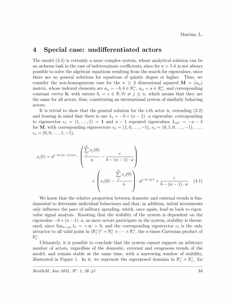
Ultimately, it is possible to conclude that the system cannot support an arbitrarynumber of actors, regardless of the domestic, external and exogenous trends of themodel, and remain stable at the same time, with a narrowing window of stability,illustrated in Figure 1. In it, we represent the superposed domains in R+

∗ × R+∗ , for

ReviSeM, Ano 2021, No. 1, 26–45 34

Martins, L.

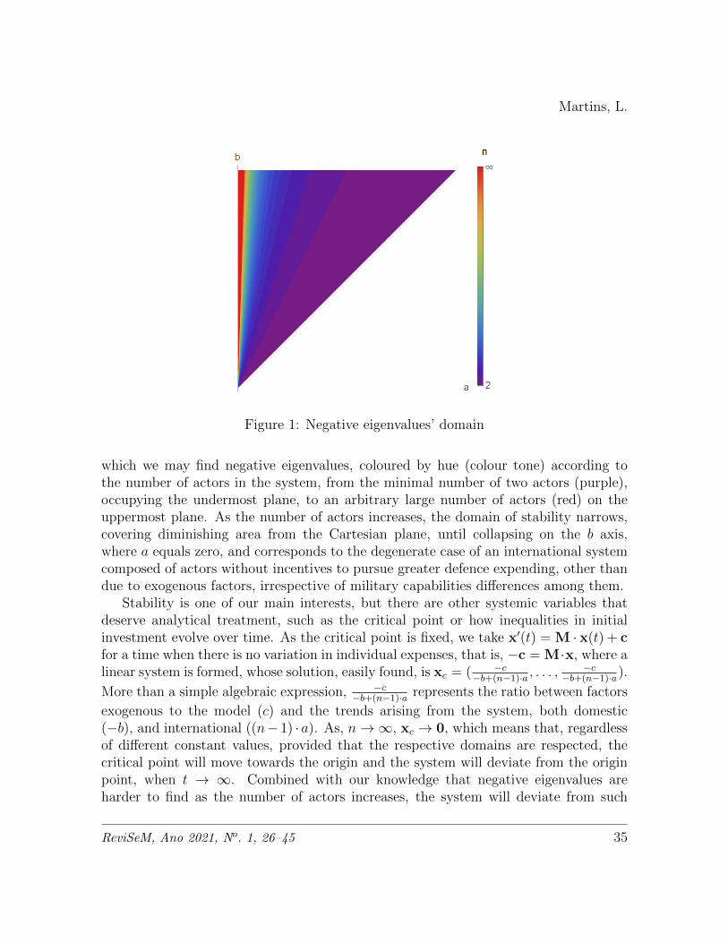
Figure 1: Negative eigenvalues’ domain

which we may find negative eigenvalues, coloured by hue (colour tone) according tothe number of actors in the system, from the minimal number of two actors (purple),occupying the undermost plane, to an arbitrary large number of actors (red) on theuppermost plane. As the number of actors increases, the domain of stability narrows,covering diminishing area from the Cartesian plane, until collapsing on the b axis,where a equals zero, and corresponds to the degenerate case of an international systemcomposed of actors without incentives to pursue greater defence expending, other thandue to exogenous factors, irrespective of military capabilities differences among them.

Stability is one of our main interests, but there are other systemic variables thatdeserve analytical treatment, such as the critical point or how inequalities in initialinvestment evolve over time. As the critical point is fixed, we take x′(t) = M · x(t) + cfor a time when there is no variation in individual expenses, that is, −c = M·x, where alinear system is formed, whose solution, easily found, is xc = ( −c

−b+(n−1)·a , . . . ,−c

−b+(n−1)·a).

More than a simple algebraic expression, −c−b+(n−1)·a represents the ratio between factors

exogenous to the model (c) and the trends arising from the system, both domestic(−b), and international ((n− 1) ·a). As, n→∞, xc → 0, which means that, regardlessof different constant values, provided that the respective domains are respected, thecritical point will move towards the origin and the system will deviate from the originpoint, when t → ∞. Combined with our knowledge that negative eigenvalues areharder to find as the number of actors increases, the system will deviate from such

ReviSeM, Ano 2021, No. 1, 26–45 35

Martins, L.

critical point, as it constitutes a source (opposed to a sink or a saddle point) of theODEs’ equilibrium point.

Investigating systemic inequality, an adequate indicator of analysis is the varianceof the values xi(t) between the actors, from solution (4.1). First, we need to averagexi(t),

n∑i

xi(t)

n= µ(t) = e(−b+(n−1)·a)t ·

n∑j

xj(0)

n− c

b− (n− 1) · a

+c

b− (n− 1) · a.

The behaviour of the average is similar to that of individual actors. Accordingto the eigenvalue λ1, the average either grows continuously or tends to c

b−(n−1)·a , whichcorresponds to situations of instability and stability, respectively, except for the singularcase when the average of the initial investments is equal to c

b−(n−1)·a .With the average, it is possible to calculate the variance,

σ2(t) =

n∑i

xi(t)−n∑jxj(t)

n

2

n⇒ σ2(t) =

n∑i

(xi(0)− µ(0))2 · e(−ba)·2t

n.

Regardless of λ1, the variance tends to 0, as t increases. Ultimately, all individualbudgets match up, despite investment differences at the start of the arms race. Indeed,the initial xi(0) investment is irrelevant to the long-term dynamics of xi(t). What theinitial investment influences is the pace at which the variation in military spending isundertaken, which assigns unique behaviours to each actor. Taking the rate of changeof the intermediate term of xi(t),

d

dt

xi(0)−

n∑j

xj(0)

n

· e(−b−a)·t

= (µ(0)− xi(0)) · (a+ b) · e(−b−a)·t.

In the situation where the i-th actor has a defence expenditure higher than theaverage of the initial investments of all the actors, there is an instant decrease in militaryexpenditures, due to the preponderance of the actor with greater investment over thegeneral average. However, it is important to note that, even here, the initial individualinvestment is related to a systemic variable, which is the average of the investments ofall the actors, at time t = 0.

ReviSeM, Ano 2021, No. 1, 26–45 36

Martins, L.

We should inquire to which domain of constants solution 4.1 holds, that is, it isstrictly greater than zero for all positive time considered. After algebraic manipulations,we find,

µ(0)(1− e−nt) + xi(0)e−nt >c

−b+ (n− 1)a(eb−(n−1)at − 1)

It is of the form f(t) > g(t), with both functions continuous and differentiable ont ∈ T . Under such properties, we may encounter maximum and minimum values, whichprovide the appropriate domain for non degenerated cases,

max(xi(0), µ(0)) ≥{

max(0,− c−b+(n−1)a

), λ1 > 0

max(0, sgn(c) · ∞), λ1 < 0

Where sgn denotes the sign function. At first, there are values of the constants(xi(0), µ(0), a, b, c, n) that do not hold for the above inequality, however, when we con-sider n→∞, it is clear that λ1 →∞ > 0 and − c

−b+(n−1)a→ 0, which means that the

inequality is satisfied for any set of valid xi(0) > 0.One interesting case arises when we consider the situation when domestic restraints

match foreign incentives. However, we are unable to simply equate both terms, as itproduces an undefined expression, since the denominator of some terms in equation 4.1match 0. Still, treating temporarily constants as variables, we are able to inquire thelimit as we approach this particular case, −b + (n − 1) → a. It is possible to find theexplicit solution, given by,

limb→(n−1)·a

xi(t) =

n∑i

xi(0)

n+ c · t+

xi(0)−

n∑i

xi(0)

n

· e−a·n·t. (4.2)

As a limit situation, the solution when λ1 → 0 is not covered by the λ1 < 0 or λ1 > 0cases, since the dominant term is ct. It is not surprising that, as the internal and externalfrequencies are the same, the exogenous factor explains the general trend of the model.For c > 0, spending tends to grow continuously, while for c < 0, investments decrease.For c = 0, xi(t) tends to the initial average of investments, the actors only balancethe initial differences around this equilibrium point, which ends up being different fromthe original critical point in value, but not in behaviour. However, not all values ofc are permitted. Following the same reasoning we applied on equation 4.1 on 4.2, wefind that the condition on the constants is max(xi(0), µ(0)) ≥ −ct, which can only beachieved when c ≥ 0, ∀t ∈ T .

ReviSeM, Ano 2021, No. 1, 26–45 37

Martins, L.

We should mention that the only stability condition for positive λ1 is when the

first term of xi(t) zeroes the dominant exponential,∑nj xj(0)

n− c

b−(n−1)·a = 0. It isthe condition in which the initial average of the system equals c

−b+(n−1)·a , with justa redistribution of individual budgets towards the critical point, where it occurs theequality of budgets between the actors. However, it is important to highlight thedifficulty in achieving stability in this case, as it is very unlikely that, in a continuousdistribution of a system taken at random, the initial average will be equivalent to− cb−(n−1)·a , that is, it corresponds to a point, but, from a Lebesgue measure perspective

on a probability space, individual points in a multidimensional Euclidean space have ameasure of 0, therefore, the probability of randomly finding the initial system in suchposition is also 0.

For systemic inequality investigation, in the special case, the average is given by,

limb→(n−1)·a

∑ni xi(t)

n=

∑nj xj(0)

n+ c · t

Nonetheless, σ2(t) still tends to 0, when t→∞.

5 General case: differentiated actors

We may tackle (3.4) not by searching exact solutions, but, rather, investigating ODEsystem’s properties that are subject to analytical investigation. For sufficiently largeshift s∗ ∈ R+

∗ , Ms∗ = M + s∗I, I being the identity matrix of dimension n by n, Ms isas strictly positive matrix, that is, corresponding entries are strictly positive, thereforewe may apply the following results on Ms∗ ,

Theorem 5.1 (Perron–Frobenius theorem). ”(a) If [matrix] A is positive, then [spectralradius] ρ(A) is a simple eigenvalue, greater than the magnitude of any other eigenvalue.(b) If A > 0 is irreducible then ρ(A) is a simple eigenvalue, any eigenvalue of A of thesame modulus is also simple, A has a positive eigenvector x corresponding to ρ(A), andany non-negative eigenvector of A is a multiple of x.”

Source: [4, p. 27]Let r be the spectral radius of matrix A, si denote the sum of elements of the i-th

row of A, S = maxi si, and s = mini si, then,

Theorem 5.2. Let A ≥ 0 be irreducible. Let x be a positive eigenvector and let γ =maxi,j(xi/xj). Then,

s ≤ r ≤ S

ReviSeM, Ano 2021, No. 1, 26–45 38

Martins, L.

and(S/s)1/2 ≤ γ.

Source: [4, p. 37-38]First, we need some additional notation. b∗i = aii and ci = bi. Moreover, we may

organise entries ai 6=j, such that a∗i 6=j ≥ a∗i 6=k,∀j ≥ k. If limn→∞ limj→n− a∗i 6=j 6= 0, the

impact of frequency of expenditures does not vanish as the number of actors increase,then limn→∞ limj→n− si = limn→∞ limj→n− b

∗i +

∑nj 6=i aij + ci − s∗ = ∞ > 0, whenever

s∗ rate of change, as n increases, is inferior to that of the divergent series. However,there are limits to how large |bi| is, and by extension s∗, because bi represents domesticdisincentives proportional to already incurred military expenses. It is clear that M isirreducible, as it may not be written as a upper triangular matrix, since there are no0 entries, therefore there is no permutation of rows and columns that produces uppertriangular matrix and theorems (5.1) and (5.2) fully apply.

From theorem (5.2), considering λmax = r,

min b∗i +n∑j 6=i

aij + ci ≤ λmax − s∗ ≤ max b∗k +n∑l 6=k

akl + ck

Since λmax ≥ min b∗i +∑n

j 6=i a∗ij + ci − s∗, we have,

λmax ≥ limn→∞

min b∗i +n∑j 6=i

a∗ij + ci − s∗ =∞ > 0

With at least one positive eigenvalue, we know that the critical point is neither a sinknor a spiral sink, resulting in not assured stability, furthermore, theorem (5.1) guaran-tees the existence of eigenvector with strictly positive entries associated to λmax that actas an attractor to points in (R+

∗ )n. However, one should notice that x′i(0) = b∗ixi(0) +∑nj 6=i aijxj(0)+ci. Organising entries ai 6=jxj(0), such that a∗i 6=jx

∗j(0) ≥ a∗i 6=kx

∗k(0),∀j ≥ k,

if limn→∞ limj→n− a∗i 6=jx

∗j(0) 6= 0, the initial impact of ”speed” of budgets’ variation does

not vanish as the number of actors increase, then limn→∞ x′i(0) > 0. Applying first or-

der approximation for ∆ ∈ R+, xi(0 + ∆) ≈ xi(0) + ∆(b∗ixi(0) +∑n

j 6=i a∗ijx∗j(0) + ci),

thus limn→∞ xi(∆) =∞. This approximation has as upper boundary the errorx′′i (η)∆2

2!,

for η ∈ [0,∆], that maximises the second order derivative [6, p. 350]. For succes-sive approximations, limt→∞ limn→∞ xi(t) = ∞. We may also see that, for each step,the military expenditure is strictly increasing, x′i(t) > 0, therefore, for any initial setxi(0) > 0, and constants that fit the non vanishing criteria, xi(t) is strictly positive andsatisfies our requirement of no negative or zero defence investments.

The critical point xc is given by Cramer’s rule,

ReviSeM, Ano 2021, No. 1, 26–45 39

Martins, L.

xc =

∣∣∣∣∣∣∣−c1 . . . a1n

.... . .

−cn ann

∣∣∣∣∣∣∣∣∣∣∣∣∣∣a11 . . . a1n...

. . .

an1 ann

∣∣∣∣∣∣∣, . . . ,

∣∣∣∣∣∣∣a11 . . . −c1...

. . .

an1 −cn

∣∣∣∣∣∣∣∣∣∣∣∣∣∣a11 . . . a1n...

. . .

an1 ann

∣∣∣∣∣∣∣

.

Applying Laplace’s determinant expansion on the i-th element xic of the xc vector,one finds, ∣∣∣∣∣∣∣∣∣∣∣

a11 . . . −c1 a1n

.... . .

.... . .

...

a1n . . . −cn . . . ann

∣∣∣∣∣∣∣∣∣∣∣∣∣∣∣∣∣∣∣∣∣∣

a11 . . . a1i a1n

.... . .

.... . .

...

a1n . . . ani . . . ann

∣∣∣∣∣∣∣∣∣∣∣

=

∑nj −cj(−1)i+jdet(Mij)∑nj aij(−1)i+jdet(Mij)

. (5.1)

However, we may interpret both dividend and divisor of (5.1) as scalar productbetween vectors, resulting in∑n

j −cj(−1)i+jdet(Mij)∑nj aij(−1)i+jdet(Mij)

=c · det(M∗)

ai · det(M∗)

=||c||||det(M∗)||cos(θ1i)

||ai||||det(M∗)||cos(θ2i)

=||c||cos(θ1i)

||ai||cos(θ2i)

Should limn→∞||c||||ai|| = 0 or cos(θ1i) = 0, xc = 0, corresponding to the respective cases

when the endogenous factors prevail over exogenous factors of the model and when thereare no exogenous factors c = 0, as, only then, the numerator of (5.1) is 0 for every entryof xc. Otherwise, there is no xc ∈ (R+

∗ )n with non-vanishing limn→∞ limj→n− a∗i 6=jx

∗j 6= 0,

for xj ∈ R+∗ , that satisfies the linear equations system corresponding to (5.1).

ReviSeM, Ano 2021, No. 1, 26–45 40

Martins, L.

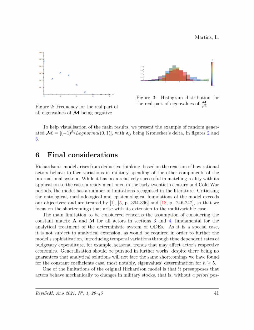
Figure 2: Frequency for the real part ofall eigenvalues of M being negative

Figure 3: Histogram distribution forthe real part of eigenvalues of M√

n

To help visualisation of the main results, we present the example of random gener-ated M = [(−1)δijLognormal(0, 1)], with δij being Kronecker’s delta, in figures 2 and3.

6 Final considerations

Richardson’s model arises from deductive thinking, based on the reaction of how rationalactors behave to face variations in military spending of the other components of theinternational system. While it has been relatively successful in matching reality with itsapplication to the cases already mentioned in the early twentieth century and Cold Warperiods, the model has a number of limitations recognised in the literature. Criticisingthe ontological, methodological and epistemological foundations of the model exceedsour objectives; and are treated by [1], [5, p. 394-396] and [18, p. 246-247], so that wefocus on the shortcomings that arise with its extension to the multivariable case.

The main limitation to be considered concerns the assumption of considering theconstant matrix A and M for all actors in sections 3 and 4, fundamental for theanalytical treatment of the deterministic system of ODEs. As it is a special case,it is not subject to analytical extension, as would be required in order to further themodel’s sophistication, introducing temporal variations through time dependent rates ofbudgetary expenditure, for example, seasonal trends that may affect actor’s respectiveeconomies. Generalisation should be pursued in further works, despite there being noguarantees that analytical solutions will not face the same shortcomings we have foundfor the constant coefficients case, most notably, eigenvalues’ determination for n ≥ 5.

One of the limitations of the original Richardson model is that it presupposes thatactors behave mechanically to changes in military stocks, that is, without a priori pos-

ReviSeM, Ano 2021, No. 1, 26–45 41

Martins, L.

sibility of engaging in behaviour different from that described by system 3.1. Nikol’skii[19] seeks to avoid the situation by recourse to control theory, conceptualising expendi-ture as controllable by one of the actors in two different models, first, on the exogenousfactor (linear model) and, second, rate of expenditure change in response to the oppo-nent current level of military stock, offering general form and conditions of solution.

The paper [20] extends the previous work and makes explicit analytical solution forspecial case of constant coefficients. Both linear and bilinear, solution is either constantor step function, with only one discontinuity. Before commenting on this finding, werefer to [17] article, which may be thought as an extension of [19] linear controlled model,since it considers that not only one, but both actors have controls on the respectiveinvestments and engage in a differential game dynamic. Their approach differs fromthat of [19], because they consider, in addition to controls, a quadratic loss functionto be minimised by the actors, but their conclusion partially converges with [20], asthey find that the solution for the control is constant. Both [17] and [20] reach modelsthat are nearly identical to the original Richardson work, but they provide importantinsight on arms race theorising, as “the coefficients of this set of equations are derivedexplicitly in terms of the parameters from each nation’s optimization in the differentialgame” [17, p. 1139]. We are inclined to conjecture new hypothesis to be tested - does asimilar conclusion happen in the bilinear case for both actors with controllable inputs ina differential game? Moreover, if analytical treatment exists, do the linear and bilinearcontrols behave similarly for the multivariate case?

Nevertheless, it is an interesting extension of the Richardson’s model, as it high-lights the effects of structural variables on the systemic behaviour. We should remem-ber that both sides of the neo-neo debate place heavy emphasis on structure and drawextensively from rational choice theory, game theory and microeconomics. Despitesuch background, the IR field still lacks thorough mathematical theorising, being theRichardson’s model one of the few exceptions. In this sense, we argue reasoning devel-oped in the present paper is not altogether separated from the focal points of IR theory.According to [25], bipolar systems are the most stable, and our conclusion corroboratepartially to this idea, as we have shown the destabilising effects caused by an increasein the number of actors, but other factors presented by Waltz are not captured byRichardson’s model, such as perfectness and completion of information.

To summarise, the extension of the original case of the Richardson’s model of armsrace between two countries to multiple actors revealed new dynamics and explanatorypossibilities, especially at the systemic level, of behaviour in international militaryspending. In this sense, it should be highlighted as the main contribution of the presentpaper the verification of the emergence of the issue of scale in the model, in which itwas observed that the system cannot support an arbitrary number of actors, without

ReviSeM, Ano 2021, No. 1, 26–45 42

Martins, L.

losing stability.

Acknowledgments

This work was supported by the Conselho Nacional de Desenvolvimento Cientıfico eTecnologico (CNPq), process no 130232/2019-0.

The author would like to thank the 2019/1 Theory of International Relations Mas-ter’s class, under Professor Alcides Vaz (IREL-UnB), for insightful discussions andsuggestions.

References

[1] Charles H. Anderton. Arms race modeling: Problems and prospects. Journal ofConflict Resolution, 33(2):346–367, 1989.

[2] Robert Axelrod and Robert O. Keohane. Achieving cooperation under anarchy:Strategies and institutions. In David A. Baldwin, editor, Neorealism and neolib-eralism: the contemporary debate, pages 85–115. Columbia University Press, NewYork, 1993.

[3] David A. Baldwin. Neoliberalism, neorealism, and world politics. In David A.Baldwin, editor, Neorealism and neoliberalism: the contemporary debate, pages3–28. Columbia University Press, New York, 1993.

[4] Abraham Berman and Robert J. Plemmons. Nonnegative Matrices in the Mathe-matical Sciences. Classics in Applied Mathematics. Society for Industrial Mathe-matics, 1987.

[5] Bernhelm Booß-Bavnbek and Jens Høyrup. Mathematics and war. Springer, 2003.

[6] William E. Boyce and Richard C. DiPrima. Equacoes Diferenciais Elementares eProblemas de Valores de Contorno. LTC, Rio de Janeiro, 9 edition, 2012.

[7] J. David Byers and David A. Peel. The determinants of arms expenditures ofnato and the warsaw pact: some further evidence. Journal of Peace Research,26(1):69–77, 1989.

[8] James E. Dougherty and Robert L. Pfaltzgraff. Contending Theories of Interna-tional Relations: A Comprehensive Survey. Longman, United States, 5 edition,2000.

ReviSeM, Ano 2021, No. 1, 26–45 43

Martins, L.

[9] Francis Fukuyama. The end of history? The national interest, (16):3–18, 1989.

[10] Joseph M. Grieco. Anarchy and the limits of cooperation: a realist critique ofthe newest liberal institutionalism. In Charles W. Kegley, editor, Controversies inInternational Relations Theory Realism and the Neoliberal Challenge, pages 151–171. Wadsworth, Belmont, 1995.

[11] G. John Ikenberry. After Victory: Institutions, Strategic Restraint, and the Re-building of Order after Major Wars. Princeton University Press, 2001.

[12] G. John Ikenberry. Reflections on after victory. The British Journal of Politicsand International Relations, 2018.

[13] Walter G. Kelley and Allan C. Peterson. The Theory of Differential Equations:Classical and Qualitative. Universitext 0. Springer-Verlag New York, 2 edition,2010.

[14] Robert O. Keohane and Lisa L. Martin. The promise of institutionalist theory.International security, 20(1):39–51, 1995.

[15] John J. Mearsheimer. The false promise of international institutions. Internationalsecurity, 19(3):5–49, 1994.

[16] John J. Mearsheimer. The tragedy of great power politics. WW Norton & Company,2001.

[17] Francois Melese and Philippe Michel. Reversing the arms race: A differential gamemodel. Southern Economic Journal, pages 1133–1143, 1991.

[18] Yael Nahmias-Wolinsky. Models, numbers, and cases: methods for studying inter-national relations. University of Michigan Press, 2004.

[19] M. S. Nikol’skii. On controllable variants of richardson’s model in political science.Proceedings of the Steklov Institute of Mathematics, 275(1):78–85, 2011.

[20] M. S. Nikol’skii. Some optimal control problems associated with richardson’s armsrace model. Computational Mathematics and Modeling, 26(1):52–60, 2015.

[21] Joseph S. Nye. Neorealism and neoliberalism. In Power in the Global InformationAge, pages 29–42. Routledge, 2004.

[22] Martin J. Osborne. An introduction to game theory. Oxford university press, NewYork, 2004.

ReviSeM, Ano 2021, No. 1, 26–45 44

Martins, L.

[23] Lewis Fry Richardson. Mathematics of war and foreign politics. In James R. New-man, editor, The World of Mathematics, volume 2. New York: Simon & Schuster,1956.

[24] SIPRI. World military expenditure grows to 1.8 trillion in2018. https://www.sipri.org/media/press-release/2019/

world-military-expenditure-grows-18-trillion-2018, 2019. Accessed:2019-06-08.

[25] Kenneth Waltz. Theory of International Politics. New York: McGraw-Hill, Inc,1979.

[26] Frank V. Zagare and Branislav L. Slantchev. Game theory and other modelingapproaches, s.d.

[27] Dina A. Zinnes and John V. Gillespie. Introduction to richardson-type processmodels. In Dina A. Zinnes and John V. Gillespie, editors, Mathematical Modelsin International Relations, pages 179–188. Praeger special studies in internationalpolitics and government, United States of America, 1976.

Submitted on November 17th, 2020.Accepted on January 6th, 2021.

ReviSeM, Ano 2021, No. 1, 26–45 45