review&document: methods(and(experiences(in(radar( … ·...
TRANSCRIPT

Review document:
Methods and experiences in radar based fine scale rainfall estimation
RainGain review document January 2013 Fine scale rainfall estimation
RainGain WP2 Page 2 of 93
En wi
Review document:
Methods and experiences in radar based fine scale rainfall estimation
Outcome of the International Workshop on “Fine-‐Scale Rainfall Estimation” of April 16, 2012 organized by KU Leuven for the RainGain project.
Report prepared by: ir. Laurens Cas Decloedt prof. dr. ir. Patrick Willems
Hydraulics division, KU Leuven
Contributed: dr. ir. Auguste Gires ParisTech
Version of January 2013

RainGain review document January 2013 Fine scale rainfall estimation
RainGain WP2 Page 3 of 93
i. Overview The document consists of three main parts, an introduction to radar technology, a part on the radar measurements and a part based on the rainfall estimation from radar measurements.
Radar technology: After the introduction, Chapter I gives a summary on the different radar technologies available and the differences in the types of radars that are used for meteorological and hydrological purposes.
Radar measurements: Chapter II discusses the different radar procedures to properly calibrate the different types of radar, while Chapter III elaborates on the different adjustment procedures to ensure correct and representative radar measurements. The influence of the radar scanning strategy on the radar measurements is discussed in Chapter IV.
Rainfall estimation: Chapter V explains the different possibilities to estimate rainfall based on radar measurements and the precautions that have to be kept in mind, while Chapter VI discusses the different adjustment procedures for the ground truthing of the rainfall estimations and the different techniques for the merging of all different data sources to obtain the best possible fine scale rainfall estimates and then concludes with the uncertainty or error estimation procedures.
The following topics will be discussed:
• Radar technology and differences in the types of radars used for meteorological purposes: o Different types of radars (X-‐ vs. C-‐ & S-‐band) o Dual versus single-‐polarisation, Doppler
• Electronic radar calibration (incl. electronic stability) • Raw radar signal corrections (e.g. clutter removal, attenuation and volume correction etc) • Radar scanning strategy (e.g. finer vs. coarser resolution etc) • Rainfall estimation:
o Based on: Reflectivity (Z), Differential reflectivity (ZDR), Differential phase (KDP) etc o Errors due to highly non-‐linear physics of radar detection of precipitation o Dependence on atmospheric conditions (rain regimes, wind, humidity, temperature, …)
• Ground truthing / adjustment: o Correction for different types of radar “errors” before adjustment based on rain gauges o Take rain gauge uncertainty into account o Several adjustment methods exist: mean field bias / Brandes correction etc o Several integration methods exist: kriging (incl/excl external drift) / Kalman filter etc o Grid-‐scale versus point scale: comparison at point scale or grid scale / urban area scale?
• Fine-‐scale rainfall estimation: o Integration of all sources: C-‐band radar, X-‐band radar, rain gauges, even microwave links o Integration requires quality of data to be considered (time and space variable) o Stochastic downscaling methods (scaling laws, fractal theory)

RainGain review document January 2013 Fine scale rainfall estimation
RainGain WP2 Page 4 of 93
ii. List of abbreviations The following abbreviations will be used throughout the document.
• Radar abbreviations:
Radar Abbreviation of ‘RAdio Detection And Ranging’, an remote sensing system based on radio waves to determine the range of backscatterers, in this document mostly referring to ground-‐based weather radars.
Calibration The electronic calibration applied to the radar to give representative reflectivity estimates of good quality.
Adjustment The adjustments made to the radar reflectivity measurements based on auxiliary data sources to give representative rainfall estimates of good quality.
X-‐Band Radar operating on a wavelength around 3 cm (wavelength of 2.5-‐4 cm, frequency of 8-‐12 GHz)
C-‐band Radar operating on a wavelength around 5 cm (wavelength of 4-‐8 cm, frequency of 4-‐8 GHz)
S-‐band Radar operating on a wavelength around 10 cm (wavelength of 8-‐15 cm, frequency of 2-‐4 GHz)
• Radar variables:
R Rainfall rate (mostly expressed in mm/hr)
Z Radar reflectivity (mostly expressed in dBZ)
ZDR Radar differential reflectivity (mostly expressed in dBZ), the value is the ratio of the horizontal and vertical reflectivity. (This value can be used as an indicator of the shape of the drops which in turn is a good estimate of average drop size).
PHIDP Radar differential phase (mostly expressed in °), the value is the difference in phase between the received horizontally and vertically orientated pulses at a given distance from the radar. The differential phase will always increase with the distance. The range derivative (specific differential phase or KDP) shows where the phase changes occur.
KDP Radar specific differential phase (mostly expressed in °/km), the value is the difference in phase between the received horizontally and vertically orientated pulses over a certain distance. Unlike most of the other parameters, which are all dependent on reflected power, the specific differential phase is a "propagation effect". It appears to be a good estimator of the rainfall rate, especially at high rainfall intensities.
RHOHV Radar copolar correlation coefficient is a dimensionless number, indicating the correlation between the horizontally and vertically reflected powers. The correlation coefficient is an indication of the uniformity of the shape and type of hydrometeors within the sampling volume. This parameter could be used to discriminate between regions of rain, the melting layer and regions of snow in radar sampling volumes.

RainGain review document January 2013 Fine scale rainfall estimation
RainGain WP2 Page 5 of 93
LDR Linear depolarization ratio is the ratio between the vertically and horizontally received reflectivity, when the radar only transmits horizontally. This is thus only possible for dual-‐polarization radars that transmit and receive horizontally and vertically polarized waves with an alternating mode. The depolarization is due to the asymmetry of the particles through which the radar beam travels. For rain, the LDR is normally very low, but can be higher in melding snow and hail or graupel.
DSD Rainfall drop size distribution (mostly expressed in mm-‐1/m³), this distribution describes the number and size of the precipitating particles, sometimes also denoted as RSD, Raindrop Size Distribution.
• Project abbreviations:
Baltrad (+) An advanced weather radar network for the Baltic Sea region, Part-‐financed by the European Union. http://www.baltrad.eu
CASA Engineering Research Center for Collaborative Adaptive Sensing of the Atmosphere, a National Science Foundation project. http://www.casa.umass.edu/
EG-‐CLIMET European Ground-‐Based Observations of Essential Variables for Climate and Operational Meteorology, a COST (European Cooperation in Science and Technology) project. http://www.eg-‐climet.org/
OPERA Operational Programme for the Exchange of Weather Radar Information, a EUMETNET project. http://www.knmi.nl/opera/
TOMACS Tokyo Metropolitan Area Convection Study for Extreme Weather Resilient Cities, a government funded project. http://www.mpsep.jp/english/index.html
UFO Ultra Fast wind sensOrs, a European research project about aviation safety through wake-‐vortex advisory systems, using ultra fast lidar, radar wind and eddy dissipation rate monitoring sensors.
http://cordis.europa.eu/search/index.cfm?fuseaction=proj.document&PJ_RCN=13112068
• Other abbreviations:
ACF Areal correction factors
ANN Artificial neural network
AP Anomalous propagation of the radar waves
ARF Areal reduction factors
BL Bartlett-‐Lewis rainfall models
BRA Brandes spatial adjustment method
CDF Cumulative distribution function
DEM Digital elevation map
GCM Global circulation model
GLM Generalized linear model
HMM Hidden Markov models

RainGain review document January 2013 Fine scale rainfall estimation
RainGain WP2 Page 6 of 93
IDW Inverse distance weighing method
KED Kriging correction method with external drift
KRE Kriging correction method with radar based error correction
KRI Kriging (as a summary of the set of kriging methods)
LAM Limited area meteorological model
MFB Mean field bias correction method
MM Markov models
NHHMM Non homogeneous hidden Markov models
NHMM Non homogeneous Markov models
NN Neural network
NS Neyman-‐Scott rainfall models
PBB Partial beam blockage
PDF Probability distribution function
QLPE Qualitative precipitation estimation
QM Quantile mapping
QPE Quantitative precipitation estimation
QPF Quantitative precipitation forecast
QQ Quantile quantile … (e.g. QQ plot, QQ transformation, etc.)
RCM Regional circulation model
RF Radio frequency
RDA Range dependant adjustment method
SNR Signal to noise ratio
TBR Tipping bucket rain gauge
VPR Vertical profile of reflectivity
WT Weather typing or types

RainGain review document January 2013 Fine scale rainfall estimation
RainGain WP2 Page 7 of 93
iii. Introduction This review document is one of the outcomes of the International RainGain workshop (April 16 2012) in Leuven on “Fine scale rainfall estimation” which fits within the scope of RainGain’s Work Package 2. The workshop was concluded with an overview of the main items discussed during the workshop and the main findings and recommendations, which formed the main topics to be included in the ‘guidelines’ for this review document. The aim of this review document is not to reproduce material that is already available in the literature or from other radar projects1 such as CASA (USA), OPERA, EG-‐CLIMET, BALTRAD, UFO (EU) and TOMACS (Japan). The document especially focuses on the use of fine-‐scale rainfall data for urban hydrological applications. (The projects mentioned are explained in the section ‘List of abbreviations’.)
One of the goals of Work Package 2 of the RainGain project is to obtain fine scale radar based rainfall estimates, fine scale both in temporal and spatial resolution. The question thus rises what these required temporal and spatial resolution should be. Discussion on this during the workshop led to the aim values chosen to be ranging from 1 till 10 minutes for the temporal resolution (preferably integrated rather than instantaneous measurements) and down to 100m for the spatial resolution.
One of the other goals of the project is to set up an interfacing between the demands of the flood modellers and forecasters and the possibilities of the radar meteorologists to deliver rainfall estimates with this spatial and temporal resolution. This document aims to bridge the gap between the expertise fields of radar meteorology and urban hydrology, drainage and flood management and control. The different steps in the radar chain are however also discussed, since it is important for urban hydrologists to know how radar rainfall measurements are obtained.
To facilitate conversations between radar meteorologists and urban hydrologists, some nomenclature is decided upon, namely:
! Radar calibration: The electronic calibration applied to the radar to give representative reflectivity estimates of good quality.
! Radar adjustment: The adjustments made to the radar reflectivity measurements to give representative rainfall estimates of good quality.
1 The project references are mentioned in section ii – ‘List of abbreviations’.

RainGain review document January 2013 Fine scale rainfall estimation
RainGain WP2 Page 8 of 93
iv. Contents i. Overview .......................................................................................................................................... 3 ii. List of abbreviations ......................................................................................................................... 4 iii. Introduction ..................................................................................................................................... 7 iv. Contents ........................................................................................................................................... 8
Chapter I. Introduction to radar technology ........................................................................................... 10 i. Working principle of a radar .......................................................................................................... 10 ii. Different wavelengths .................................................................................................................... 11 iii. Dual polarization radars ................................................................................................................. 12 iv. Doppler radars ............................................................................................................................... 14 v. Phased array radars ........................................................................................................................ 14 vi. Microwave links ............................................................................................................................. 15
Chapter II. Electronic calibration of the weather radar ........................................................................... 17 i. Calibration of total radar chain ...................................................................................................... 17 ii. Calibration of receiver chain .......................................................................................................... 18
Chapter III. Different corrections to the raw radar signal ......................................................................... 19 i. Noise cut off ................................................................................................................................... 19 ii. Volume correction .......................................................................................................................... 19
Volume and VPR correction methods ................................................................................................ 19 Anomalous propagation correction methods .................................................................................... 21 Partial beam blockage correction methods ....................................................................................... 22
iii. Attenuation correction ................................................................................................................... 24 Based on a reflectivity – specific attenuation relation (Hitschfeld-‐Bordan algorithm) ...................... 24 Based on PHIDP and KDP – specific attenuation relation ...................................................................... 25 Other attenuation correction methods .............................................................................................. 26
iv. Clutter correction ........................................................................................................................... 27 Clutter map ........................................................................................................................................ 27 Doppler measurements ..................................................................................................................... 28 Statistical clutter removal .................................................................................................................. 28 Dual polarization radar measurements .............................................................................................. 29 Combinations ..................................................................................................................................... 29
Chapter IV. Influence of the radar scanning strategy on the radar estimates .......................................... 30
Chapter V. Estimation of rainfall rates from radar measurements .......................................................... 34 i. Rainfall estimation from single polarization radar data ................................................................. 34 ii. Rainfall estimation from dual polarization radar data ................................................................... 35 iii. Errors in the radar based rainfall estimation assumptions ............................................................ 36 iv. Errors in the radar rainfall measurements ..................................................................................... 37
Chapter VI. Combining radar rainfall estimates with other rainfall measurements ................................. 39 i. Errors in the point rainfall measurements ..................................................................................... 40 ii. Resolution differences in the rainfall measurements .................................................................... 42

RainGain review document January 2013 Fine scale rainfall estimation
RainGain WP2 Page 9 of 93
Interpolation and upscaling methods ................................................................................................ 43 Downscaling methods ........................................................................................................................ 44
iii. Comparison methods ..................................................................................................................... 59 Methods accounting for the differences between the measurements ............................................. 59 Methods incorporating the differences between the measurements ............................................... 62
iv. Adjustment or integration principles and methods ....................................................................... 62 Adjustment methods ......................................................................................................................... 62 Integration methods .......................................................................................................................... 64 Comparison of different methods ...................................................................................................... 66
v. Incorporating uncertainties when merging rainfall data ............................................................... 68 Kalman filter ....................................................................................................................................... 69 Kriging methods ................................................................................................................................. 69 Radar QPE methods incorporating error/uncertainty assessment .................................................... 69
vi. Conclusion ...................................................................................................................................... 70
List of references ........................................................................................................................................ 71 i. List of figures .................................................................................................................................. 91 ii. List of tables ................................................................................................................................... 92

RainGain review document January 2013 Fine scale rainfall estimation
RainGain WP2 Page 10 of 93
Chapter I. Introduction to radar technology
i. Working principle of a radar The name Radar is an acronym for “RAdio Detection And Ranging” and it was developed shortly before and during World War II, where it was part of the anti-‐aircraft defence mechanism due to its ability to detect airplanes. The radar operators however noticed that the images contained echoes from rainfall and other obstacles. After the war, the radar technology was further developed, also in a scientific environment, with specific interest for the meteorological use of the radar technology.
A radar mainly consists of an antenna and receiver unit, as well as some processing hard-‐ and software behind it. The radar antenna sends out electromagnetic pulses, which are scattered in all directions by all sorts of objects, be it planes, raindrops, buildings etc. A portion of the emitted energy is reflected back to the radar receiver, where the returning power is measured. This process is illustrated in Figure 1.
Figure 1: Working principle of a weather radar (after Cain, 2002)
Assuming that only Rayleigh scattering is occurring in the scanning volume (which should mainly be the case given the size of the hydrometeor and the signal wave length), the received power is expressed by the radar equation (I-‐1) according to Battan (1973). The equation can be rewritten to the weather radar equation (I-‐2) from which the radar reflectivity Z can be deduced based on the measured returning power Pr.
𝐏𝐫 =𝐏𝐭𝐆𝟐𝛌𝟐𝛔𝐢𝟒 𝛑 𝟑𝐫𝟒
I-‐1
Where: P! = the power received by the radar, P! = the power transmitted by the radar, G = the gain of the antenna, λ = the wavelength,
σ! = the targets cross section and r = the target range.
𝐏𝐫 = 𝐂 𝐊𝐰 𝟐 𝐙𝐫𝟐 I-‐2
Where: C = the radar constant, K! = a coefficient related to the dielectric constant of water and Z = the radar reflectivity value.

RainGain review document January 2013 Fine scale rainfall estimation
RainGain WP2 Page 11 of 93
It can be shown that the radar reflectivity Z and the rainfall rate R are related to the Drop Size Distribution (DSD) by equations I-‐3 and I-‐4 respectively (e.g. Marshall and Palmer, 1948 or Uijlenhoet, 2001). Rainfall estimation from radar measurements is thus based on the relationship between Z and R through a power law relation, see equation I-‐5, with two constants that have to be fitted. More information on rainfall estimation will be given in Chapter V.
𝐙 ~ 𝐧 𝐃 .𝐃𝟔.𝐝𝐃 I-‐3
𝐑 ~ 𝐧 𝐃 .𝐃𝟑. 𝐯 𝐃 .𝐝𝐃 I-‐4
Where n(D) is the drop size distribution, D is the equivalent spherical diameter and v(D) is the hydrometeor fall speed.
𝐙 = 𝐚.𝐑𝐛 I-‐5
ii. Different wavelengths Worldwide, several different wavelength bands are used for operational meteorological radars.
These consist of the S, C and X bands. The S-‐band consists of wavelengths around 10cm, the C-‐band wavelengths lay around 5cm and the X-‐band wavelengths around 3cm. More specific details can be found in Table 1, where also the radar operating frequency is mentioned. The choice of the wave length for the radar (λ) also has some consequences on the size of the antenna. Indeed the beam width θ (°) is related to the wavelength, the antenna efficiency ea (typically at least 0.8) and its diameter da (m) by formula I-‐6.
aadeλ
πθ
180= I-‐6
Given that θ is usually approximately equal to 1°, it appears the size of S band radar antenna is roughly 6-‐10 m (meaning that the installation and maintenance costs are elevated), the C band one is of 3-‐5 m and X-‐band one of 1-‐2 m.
Table 1: Radar characteristics for the different wavelength bands
S-‐band C-‐band X-‐band Wavelength [cm] 8 -‐ 15 4 -‐ 8 2,5 -‐ 4 Frequency [GHz] 2 -‐ 4 4 -‐ 8 8 -‐ 12 Antenna size [m] 6 -‐ 10 3 -‐ 5 1 -‐ 2
The C-‐band radars offer a range of qualitative precipitation estimation (QLPE) up to 250km, whereas for quantitative precipitation estimation (QPE) the range is somewhat limited to about 150km, however, QPE could be possible up to nearly 200km depending on the type and specifications of the C-‐band radar and with the necessary adjustments. The X-‐band radars have a shorter range, going up to 100km for QLPE and up to 50km for QPE, depending on the type and specifications of the X-‐band radar.
An X-‐band radar is thus mostly used to cover a smaller area with a higher spatial resolution. The spatial resolution of a C-‐band radar is however not necessarily coarser than that of an X-‐band radar. The resolution is not a function of the wavelength, but of the used length of the radar pulse and the width of

RainGain review document January 2013 Fine scale rainfall estimation
RainGain WP2 Page 12 of 93
the radar beam as well as the scanning strategy. Where the C-‐band radar is mostly used to cover a greater area than the X-‐band radar, an especially dedicated scan of the C-‐band could be used to get a finer spatial resolution for the area close to the radar. More information on this is given in Chapter IV.
If the received radar signal falls back to the noise level, the content is totally lost. This could possibly even further limit the range of the X-‐band radars for extreme events, since they suffer more from attenuation. For these events, the added value of the S-‐ and C-‐band radars is clear. It is however not necessarily always the case that the C-‐band radar data is more reliable than the X-‐band data.
Hence it appears that the choice of radar band is a trade off between the surface needed to be monitored, the desired resolution, the typical type of rainfall and the cost of maintaining the network. The national meteorological services mostly use S-‐ or C-‐band to offer nationwide coverage, since the X-‐band radar has a more limited range. In America mostly S-‐band radars are used, whereas in Europe C-‐band radars are more common.
iii. Dual polarization radars With a dual polarization (or dual-‐pol) radar, the transmitter sends radar signals with perpendicular polarizations, horizontal and vertical. In the conventional single polarization radars, the signal transmission is limited to one direction, mostly the horizontal. See Figure 2 for a comparison of the two mechanisms. With two polarized signals, it is possible to derive several new additional parameters which give extra information on the precipitation type, size and shape. The polarimetric parameters will be discussed below and more information on dual polarization radar characteristics can be found in the literature, e.g. Bringi and Chandrasekar (2001).
Figure 2: Working principle of a conventional (single, horizontal polarization) radar
versus a dual polarization (horizontal and vertical) radar (Source: NOAA)
The additional dual polarization parameters consist of:
• ZDR The differential reflectivity • ΦDP The differential phase (PHIDP)

RainGain review document January 2013 Fine scale rainfall estimation
RainGain WP2 Page 13 of 93
• KDP The specific differential phase • ρHV The copolar correlation coefficient (RHOHV) • LDR The linear depolarization ratio
The differential reflectivity ZDR is mostly expressed in dB. The value is the ratio of the horizontally and vertically reflected powers (see equation I-‐7). The value can be used as an indicator of the shape of the drops. Whereas a ZDR around zero represents hydrometeors which are nearly circular, a positive value represents horizontally oriented drops and a negative value represents vertically oriented drops. This is shown in Figure 3. The shape of the drops is in turn is a good estimate of average drop size since larger drops are mostly more oblate. The presence of hail is also easily discovered in combination with the reflectivity. Hailstones generally have a bigger diameter than rain, resulting in a higher reflectivity. Hailstones however also have a more spherical shape than large raindrops, due to their tumbling motion as they fall, resulting in a ZDR value that is close to zero.
10.log HDR
V
ZZZ
⎛ ⎞= ⎜ ⎟
⎝ ⎠ I-‐7
Figure 3: Impact of hydrometeor shape on the polarimetric variable ZDR
The differential phase PHIDP is mostly expressed in degrees (°). The value is the difference in phase between the received horizontally and vertically orientated pulses at a given distance from the radar. The differential phase will thus always increase with the distance.
The specific differential phase KDP is mostly expressed in °/km. The value is the difference in phase between the received horizontally and vertically orientated pulses over a certain distance. KDP is thus the range derivative of the differential phase and shows where exactly the changes in differential phase occur. Unlike most of the other parameters, which are all dependent on reflected power, the differential phase and the specific differential phase are "propagation effects"; this makes KDP unaffected by attenuation and independent of the radar calibration. The value of KDP is high in areas with high rainfall intensities because in these areas the phase shift between the horizontally and vertically polarized signals will be high. This is however only the case if the precipitation consists mostly of rain, since hail produces a lesser phase shift and thus a less high value of KDP. These regions with hail can however be filtered out by comparison with the reflectivity values.
The copolar correlation coefficient RHOHV is a dimensionless number, indicating the correlation between the horizontally and vertically reflected powers. The correlation coefficient is an indication of the uniformity of the shape and type of hydrometeors within the sampling volume, as it is close to 1 for a uniform volume and decreases rapidly for non-‐uniform sampling volumes. According to Matrosov et al

RainGain review document January 2013 Fine scale rainfall estimation
RainGain WP2 Page 14 of 93
(2007), RHOHV in rain is generally greater than 0.95, in snow greater than 0.85 and it is significantly smaller in the melting layer. This parameter could thus possibly be used to discriminate between regions of rain, the melting layer and regions of snow in radar sampling volumes.
The linear depolarization ratio LDR is the ratio between the vertically and horizontally received reflectivity, when the radar only transmits horizontally. This is thus only possible for dual-‐polarization radars that transmit and receive horizontally and vertically polarized waves with an alternating mode. The depolarization is due to the asymmetry of the particles through which the radar beam travels. For rain, the LDR is normally very low, but can be higher in melding snow and hail or graupel.
In order to get a complete and correct picture of the actual rainfall characteristics, the polarimetric variables should be compared and give consistent results. It is clear that with dual polarization radars, more details about the rainfall characteristics can be captured compared to conventional single polarization radars.
iv. Doppler radars Radars with Doppler capability are able to measure the radial velocity of the scatterers, due to the induction of a frequency shift (because of the Doppler effect) over two consecutive radar scans (mostly 2 special Doppler scans close together). They produce 2 extra parameters, which characterize the distribution of the velocities of the backscatterers within the different radar sampling volumes. More information on the Doppler radar characteristics can be found in Bringi and Chandrasekar (2001) and Doviak and Zrnic (2006). The new Doppler parameters consist of:
• Vr The mean Doppler radial velocity • σV The Doppler spectrum width
The mean Doppler radial velocity Vr is expressed in m/s. The value is the mean of the velocities of the different backscatterers within the sampling volume. The mean radial velocity of the hydrometeors is strongly influenced by the wind speed and direction, whereas the radial velocity of non-‐meteorological echoes (excluding birds, insects and planes) mostly consist of near zero values. This gives Doppler radars, within a certain extent, the ability to distinguish between stationary clutter and hydrometeors. This will be discussed further in Chapter III -‐ iv. Clutter correction.
The Doppler spectrum width σV is also expressed in m/s. The value denotes the standard deviation of the distribution of the mean Doppler radial velocity within the volume. A lower standard deviation denotes a more uniform scanning volume, whereas a higher value indicates a less uniform volume, possibly with different types of hydrometeors mixed together. Higher standard deviations might also indicate the presence of clutter in the volume, as clutter has a near zero velocity.
v. Phased array radars One of the main drawbacks of the conventional radar systems is the mechanical scanning motion. Weather radars without moving parts would be a better alternative from maintenance and operational point of view. During the scanning time, a reasonable high amount of time is possibly used to scan regions where no rain is present. It would thus be an advantage to scan certain regions more frequent

RainGain review document January 2013 Fine scale rainfall estimation
RainGain WP2 Page 15 of 93
or in more detail, while scanning the other regions faster or less frequent. With the conventional mechanically steered radar dishes, this is very challenging.
Since the 1950’s, a new kind of radar design has been proposed, replacing the mechanical steering of one antenna by the electronic steering of multiple antenna units. Fenn et al. (2000) gives an overview on the development of the phased array radar technology. The principle of phased array radars is the electronic phasing of individual array antenna units in order to form one radar beam (Parker and Zimmermann 2002a and b). A phased array antenna is a group (array) of antennas in which the relative phases of the respective signals feeding the antennas are varied in such a way that the effective radiation pattern of the array is reinforced in a desired direction and suppressed in undesired directions. So instead of using only one antenna, a phased array radar has multiple antennas, placed in a specific structure.
There are mainly two different working mechanisms of the phased array radar, called Passive and Active Electronically Scanned Array (PESA and AESA), (Parker and Zimmermann 2002a and b). The main difference is the microwave feed to the antenna, with a PESA system, one main radio frequency (RF) source is used to feed the different transmitting units. With an AESA system, each transmitter has its own RF source, which ensures the operational reliability of these systems, as different RF sources may fail, while the radar as a whole will still work.
The phased array radar technology is mostly used by the military for its ability to keep an eye on several different targets, as with, for example, the Aegis combat system (Gregers-‐Hansen 2004), a so called ‘integrated naval weapons system’, which uses several phased array radars on the sides of army vessels to track and guide multiple weapons at the same time while still being able to monitor the movements of other ships and even aircrafts within the ships proximity.
Phased array radars have not really been introduced into weather radar research, mainly because of the high manufacturing costs of these radars. Recently, under impulse of new developments in the radar manufacturing and research programs such as CASA, these technologies are more and more starting to find their way into the weather radar community.
Several of the advantages have already been mentioned above, such as the ability to focus on a specific location (or specific locations) without the need to go through the entire scanning procedure. The mechanical steering has now also been replaced by a more reliable electronic steering mechanism. The main drawback until now was the cost of these phased array radars. There are however questions about the operational sensitivity for rainfall estimation purposes, which will have to be investigated further.
vi. Microwave links A microwave link consists of two antennas, one sending and one receiving unit, typically a few hundred meters up to fifteen kilometres apart. Microwave links are used for mobile telephone communication, they operate around a frequency of 7-‐40 GHz and the link length is mostly limited to a maximum of 5-‐10km. There is quite a dense network available in some countries, however, in others, this might be limited. As an estimate of the density of the microwave link network, a density of at least 0.3 links/km² can be assumed for European countries, according to Chwala et al. (2012). For example, in the

RainGain review document January 2013 Fine scale rainfall estimation
RainGain WP2 Page 16 of 93
Netherlands (35.500 km²) the total number of link paths is at least 8000 and for many of those link paths, the microwave links measure in both directions (Overeem et al., 2013).
The information sent over these links also has to travel through rain, which causes attenuation of the signal. The magnitude of the received power is mostly stored by the network operators and can thus be used to calculate the total integrated attenuation over the link path, from which the path averaged rainfall intensity can be estimated. Olsen et al. (1978) showed that the relation between rain rate R in mm/h and attenuation A in dB/km can be approximated by the power law equation 𝐴 = 𝑎.𝑅!. The constants a and b primarily depend on the frequency of the propagating wave, but also on the drop size distribution (DSD) and the temperature.
Research in this field started with research setups (e.g. Ruf et al. (1996), Holt et al. (2003), Rahimi et al. (2003, 2004 and 2006), Kramer et al. (2005), Upton et al. (2005), Grum et al. (2005), Leijnse et al. 2007a, among others), but in recent years, data from commercial cellular networks have been used to estimate rainfall intensities (e.g. Messer et al. (2006), Leijnse et al. (2007b), Zinevich et al. (2008), Overeem et al. (2011 and 2013), Chwala et al. (2012), among others). A limitation is the availability of the data, which could range from (near) real-‐time even up to only on a daily or weekly basis. Moreover, it can be hard to gain access to commercial microwave link data.
The microwave links can be used as a standalone estimator of the rainfall (e.g. Leijnse et al. 2007b, Zinevich et al. 2008), or can be combined with rain gauges and even the radar measurements (e.g. Cummings et al. 2009) to give better rainfall estimations at ground level. The links can also be used as an attenuation indicator for attenuation correction of the radar measurements. The network of these links is mostly denser over urban areas than elsewhere, which could thus be an advantage for the correction of the radar estimates for urban hydrological applications since there are mostly only a limited number of rain gauges available in the city centre. Other advantages of microwave links are that they are mostly clutter free and very close to the ground compared to radar scans. Finally, the power law equation used to compute rainfall intensity from attenuation is almost linear, whereas the Z-‐R relation employed in radar meteorology is nonlinear.

RainGain review document January 2013 Fine scale rainfall estimation
RainGain WP2 Page 17 of 93
Chapter II. Electronic calibration of the weather radar Electronic radar calibration is the electrical calibration of the reflectivity of the radar, so no adjustments to gauge information or any other corrections (attenuation or volume correction, etc) are done in this step. The electronic calibration just makes sure the received reflectivity for a given volume in space and time is the correct reflectivity for that volume.
Several different techniques can be used alone or in combination to maintain a good electronic calibration of the radar’s sender and receiver chain. Some techniques focus only on one of the two chains, while others asses the quality of the sender and receiver chain in total. The performance of the electronic calibration is mostly monitored by reapplying one or several of these techniques after a period of time to maintain a good calibration. Radar calibration checking frequencies mostly range from once a day or week to once a month.
i. Calibration of total radar chain Methods assessing the calibration of the total radar signal chain:
• Reflectivity of known clutter points This method implies that one or more fixed clutter points are clearly visible within the radar image, these points can be buildings, towers, chimneys etcetera and have a known reflectivity which is mostly very stable under normal conditions. For these points, the reflectivity is monitored over time and an offset in the reflectivity value gives an indication of a possible offset in the radar calibration. See Borowska and Zrnic (2012) and Silberstein et al (2008) for more details.
• Vertical radar scan This method implies that a dual polarization radar is used and that it is raining, since the vertical scan is used to calibrate the polarimetric variable ZDR by the droplet shape. For a vertical scan, one would theoretically predict a ZDR value of zero, because of the expected similarity of the drop dimensions in the horizontal plain, since all droplets have the highest probability to be nearly circular. References: Bringi and Chandrasekar (2001) and Gorgucci et al (1999). Even if the radar isn’t able to scan in a vertical direction (due to mechanical restrictions or time restrictions on the scanning strategy), it is possible to use a separate vertical profiling radar (Williams et al 2005) or even use the measurements with the highest (nearest to vertical) elevation angle available (Bechini et al 2008 or Ryzhkov et al. 2005a).
• Self-‐consistency of the radar variables This method implies the use of the self-‐consistency property of the horizontal reflectivity Z, the differential reflectivity ZDR, the differential propagation phase PHIDP and the specific differential phase KDP. This method needs the polarimetric radar parameters, making it unusable for single-‐pol radars. The principle was first noted by Gorgucci et al. (1992), and from this principle, methods for radar calibration were developed by e.g. Gorgucci et al. (1992), Goddard et al. (1994), Scarchilli et al. (1996), Illingworth and Blackman (2002), Vivekanandan et al. (2003), Ryzhkov et al. (2005), Gourley et al. (2009) among others.

RainGain review document January 2013 Fine scale rainfall estimation
RainGain WP2 Page 18 of 93
• Radar to radar comparison This method implies that a certain volume is scanned by two different radars. For this volume, the reflectivity values can thus be compared and should give similar results. An offset in the difference between the two radars however does not reveal which one of the two is wrongfully calibrated and thus this method requires more effort to determine the faulty calibration and the specific cause of the offset. Different radar merging methods exist, such as Zhang et al. (2005) and Lakshmanan et al. (2006), where the reflectivity from different radars can be compared. These methods are however not made for real time monitoring of the calibration performance of the different radars.
ii. Calibration of receiver chain Methods assessing only the calibration of the radar receiver chain:
• Emitting power of the sun This method implies that the sun is visible in the radar image. Since the emitting power of the sun is monitored by several institutes -‐ such as the Dominion Radio Astrophysical Observatory (DRAO) in Canada -‐ the value can be compared to the reflectivity measured by the radar for the region where the sun lies within the scanning area. The comparison of the two gives an indication of the quality of the calibration and the need to recalibrate the radar if there is a significant offset. The method was firstly proposed by Whiton et al. (1976). Among others, Rinehart (2004), Ryzhkov et al. (2005) and Holleman et al. (2010) describe possibilities of using the sun as a calibration tool for the receiver chain of the radar.
The expected reflectivity of the sun can also be obtained by measuring the solar power with another radar nearby (possibly even operating at another wavelength) and by calculating the expected reflectivity for the first radar out of the reflectivity of the other radar. This however requires the second radar to be correctly calibrated.
• Introducing a known signal in the wave guide This method implies that some sort of device induces a known signal into the antenna’s wave guide; therefore this device should be mounted on to the radar antenna. Since the signal has a known strength, the expected radar measurement can be calculated and compared to the actual measurements. This can be used to assess and if necessary correct the radar calibration (Manz et al. 2000).
In an operational context, several of these (and perhaps also other) calibration procedures mentioned are used in combination to monitor the performance of the electronic calibration. Each of these techniques are mostly reapplied after a certain interval time, depending from both the technique and the radar owner.

RainGain review document January 2013 Fine scale rainfall estimation
RainGain WP2 Page 19 of 93
Chapter III. Different corrections to the raw radar signal Raw radar signal corrections mostly include some kind of cut off of the noise on the radar signal, removal of remaining clutter in the radar image, correction for attenuation of the radar signal and volume or vertical profile correction. These different corrections will be discussed in the following sections. Note: The ideal radar measurement processing chain will be a future outcome of the OPERA project.
i. Noise cut off This part will only be discussed very briefly, as most operational radar systems have their own noise cut off algorithm preinstalled and advised settings are given by the manufacturer. However, these settings are important, because once the radar signal falls back to this noise level, the signal is totally lost and there is no way to reconstruct the weather echoes from the signal.
The conventional way to filter out noise from the measurements is to set a cut off threshold below which the measurements will be removed. There are however also other approaches, such as statistical separation of the signal and noise fields (e.g. Pegram et al, 2011).
ii. Volume correction Under this section, a series of correction mechanisms will be discussed to solve problems mainly caused by the influence of the measurement principles and the environment on the remote sensing technology. These problems consist of the influence of increasing radar measuring height, increasing radar sampling volume, the effect of (partial) beam blockage, the effect of anomalous propagation, etcetera… All these different sources could give serious over-‐ and underestimations of the rainfall rate at ground level. They will be grouped and their correction mechanisms will be discussed.
Volume and Vertical profile of reflectivity (VPR) correction methods
The need for volume and vertical profile corrections are caused by the increasing measuring height of the radar and the increasing volume sampled by the radar. The radar reflectivity does not necessarily relate to the rainfall at ground level. Several issues may occur when interpreting the reflectivity aloft as the rain rate on ground level, such as evaporation, see Figure 4 (1), condensation or coalescence (2), partial beam filling (3) or even overshooting of the rain (4), but also sublimation, riming, aggregation, and breakup can seriously change the characteristics of the rainfall near the ground (Doviak and Zrnic, 1993, Delobbe, 2006).
Figure 4: Several problems caused by the measuring height and volume of the radar, such as evaporation (1), condensation
or coalescence (2), partial beam filling (3) or even overshooting of the rain (4) (after Delobbe, 2006).

RainGain review document January 2013 Fine scale rainfall estimation
RainGain WP2 Page 20 of 93
Another factor affecting the need for volume and VPR correction is the temperature gradient in the atmosphere. At higher altitudes, above the freezing level, precipitation forms as snowflakes, whereas at lower altitudes, the snowflakes start to melt. The melting process (around and below the freezing level) affects the radar measurements, as the reflectivity is related to the size of the backscatterers and their intrinsic reflectivity. Snowflakes have a lower reflectivity (about 5 times lower, as the dielectric constant (|K|² value) in formula I-‐2 is 0.197 for snow versus 0.93 for liquid water) but they are bigger than raindrops with the same water volume. As the snowflakes start to melt, their outer layer becomes liquid which seriously increases their reflectivity signatures, as the radar sees very big raindrops. The principle of bright band formation is shown in Figure 5.
Figure 5: Principle of bright band formation below the 0°C line: left) microphysical formation of the bright band,
right) consequences on the radar VPR, idealized reflectivity vs. height diagram (adapted from the North Carolina State University website)
The bright band phenomenon occurs when the radar beam passes through the region around the melting layer, which is higher up in the atmosphere in summer, but closer to the surface in winter. The bright band could thus seriously affect the radar images if not corrected for. An example of the influence of the bright band on radar data at Wideumont, Belgium (C-‐band radar operated by the Royal Meteorological Institute, RMI) is shown in Figure 6.
Figure 6: Bright band phenomenon in radar images: a) Radar image from Wideumont (Belgium) affected by Bright band, b) vertical cut from the same radar image from the radar to the north (towards De Bilt, the Netherlands) (source: RMI)
VPR correction aims to estimate the reflectivity at ground level from the measured reflectivity aloft and thus to estimate the precipitation at ground level. During convective precipitation cases, the vertical profile of reflectivity is more uniform, whereas during stratiform events, the effect of non-‐uniform VPR is more pronounced, even more so when the radar measurements are located in the bright band region. VPR correction is sometimes also used in combination with PBB correction methods, see further.

RainGain review document January 2013 Fine scale rainfall estimation
RainGain WP2 Page 21 of 93
Numerous methods have been proposed to correct the radar measurements for these non-‐uniform VPR issues, both in research and operational conditions. The general solution is to estimate the form of the current vertical profile of reflectivity and to use this information to estimate the reflectivity at ground level. Several approaches can be used to determine this profile, by using either climatological profiles, local profiles close to the radar (e.g. Kitchen et al., 1994; Germann and Joss, 2002) or from the ratios of radar reflectivity values from different elevation angles by using an inverse theory (Andrieu and Creutin, 1995; Vignal et al., 1999). Other methods mostly rely on the identification of the bright band and extrapolate downwards from there. An overview on bright band identification methods is given in Rico-‐Ramirez and Chucky (2007). Germann et al. (2006) and Bellon et al. (2007) assessed the quality of the VPR correction methods.
Anomalous propagation correction methods
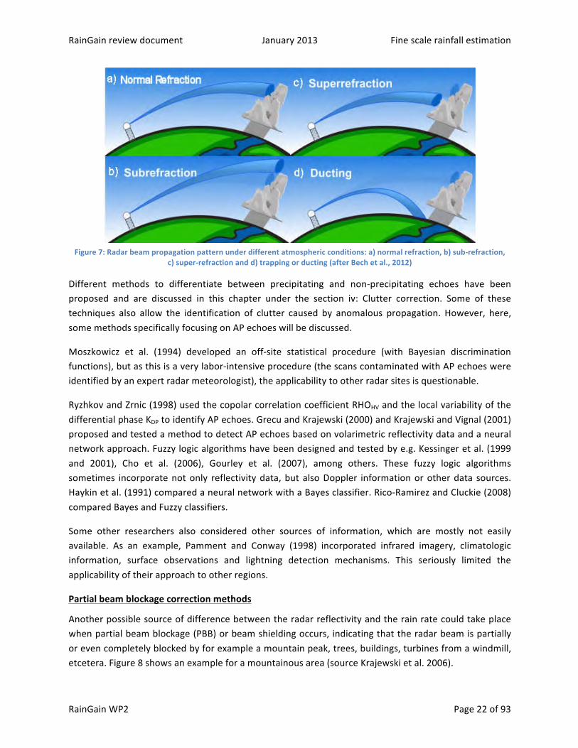
When the weather conditions are unfavorable, the propagation of the radar beam through the atmosphere could result in so called anomalous propagation (AP). During these circumstances, the radar waves are deflected from their usual path due to the refractivity of the atmosphere, causing echoes, a sort of ‘ground clutter’. According to Pratte et al. (1995), the vertical gradient of the refractivity N (dN/dh) is the key factor to determining whether AP will occur. Even more, the lowest couple of hundred meters above the radar are of particular importance. Four different atmospheric conditions leading to different propagation modes (e.g. Steiner et al., 2002 and Bech et al., 2012) can be distinguished and their effects on the radar beam are shown in Figure 7.
a) Normal refraction: radar beam is not deflected (0 m-‐1 < dN/dh < -‐0.0787 m-‐1) b) Sub-‐refraction: radar beam is deflected upwards (dN/dh > 0 m-‐1) c) Super-‐refraction: radar beam is deflected downwards (-‐0.0787 m-‐1 < dN/dh < -‐0.157 m-‐1) d) Trapping or ducting: extreme case of super-‐refraction (dN/dh > -‐0.157 m-‐1)
From these four, severe cases of super-‐refraction may cause AP clutter problems, while during atmospheric conditions leading to trapping or ducting, extensive AP clutter signatures are observable in the radar data. More information on the refraction properties can be found in Steiner et al. (2002) and Patterson (2008).
The AP echoes are, opposed to normal ground clutter, neither (nearly) constant over time (e.g. Tatehira and Shimizu, 1978 and 1980, Sirmans and Dooley, 1980) nor confined to the proximity of the radar and can thus be observed at any distance. They can exhibit precipitation-‐like patterns, such as growth, decay and motion (e.g. Johnson et al., 1975 and Weber et al., 1993).
RainGain review document January 2013 Fine scale rainfall estimation
RainGain WP2 Page 22 of 93
Figure 7: Radar beam propagation pattern under different atmospheric conditions: a) normal refraction, b) sub-‐refraction,
c) super-‐refraction and d) trapping or ducting (after Bech et al., 2012)
Different methods to differentiate between precipitating and non-‐precipitating echoes have been proposed and are discussed in this chapter under the section iv: Clutter correction. Some of these techniques also allow the identification of clutter caused by anomalous propagation. However, here, some methods specifically focusing on AP echoes will be discussed.
Moszkowicz et al. (1994) developed an off-‐site statistical procedure (with Bayesian discrimination functions), but as this is a very labor-‐intensive procedure (the scans contaminated with AP echoes were identified by an expert radar meteorologist), the applicability to other radar sites is questionable.
Ryzhkov and Zrnic (1998) used the copolar correlation coefficient RHOHV and the local variability of the differential phase KDP to identify AP echoes. Grecu and Krajewski (2000) and Krajewski and Vignal (2001) proposed and tested a method to detect AP echoes based on volarimetric reflectivity data and a neural network approach. Fuzzy logic algorithms have been designed and tested by e.g. Kessinger et al. (1999 and 2001), Cho et al. (2006), Gourley et al. (2007), among others. These fuzzy logic algorithms sometimes incorporate not only reflectivity data, but also Doppler information or other data sources. Haykin et al. (1991) compared a neural network with a Bayes classifier. Rico-‐Ramirez and Cluckie (2008) compared Bayes and Fuzzy classifiers.
Some other researchers also considered other sources of information, which are mostly not easily available. As an example, Pamment and Conway (1998) incorporated infrared imagery, climatologic information, surface observations and lightning detection mechanisms. This seriously limited the applicability of their approach to other regions.
Partial beam blockage correction methods
Another possible source of difference between the radar reflectivity and the rain rate could take place when partial beam blockage (PBB) or beam shielding occurs, indicating that the radar beam is partially or even completely blocked by for example a mountain peak, trees, buildings, turbines from a windmill, etcetera. Figure 8 shows an example for a mountainous area (source Krajewski et al. 2006).

RainGain review document January 2013 Fine scale rainfall estimation
RainGain WP2 Page 23 of 93
Figure 8: Schematic representation of radar beam blockage occurrence in mountainous areas with a frontal view from the
radar (top left) and a side view (main picture) (after Krajewski et al. 2006)
When the radar beam patterns interact with the topography, partial beam blockage (PBB) may occur. Besides the obvious ground clutter affection at the interaction areas, the regions behind these ground clutter points are also affected due to the PBB. Different methods for the correction of radar rainfall estimates suffering from PBB exist and the different groups of methods will be discussed hereafter.
With single polarization radars, most methods used digital elevation models (DEMs) for the correction of PBB. But even within this class, different approaches are possible.
One way is to combine the DEMs with the radar scanning strategy to identify which sectors in the radar image suffer from PBB and to correct these sectors with reflectivity data from the higher elevation angles or extrapolating these measurements downwards using VPR (vertical profile of reflectivity) correction methods (e.g., Andrieu et al., 1997, Creutin et al., 1997, Seo et al., 2000, Dinku et al., 2002, Langston and Zhang, 2004, Lang et al., 2009, among others). The identification of the affected radar beams could even be done by integrating geographical information systems (GIS) (e.g. Kucera et al., 2004 and Krajewski et al., 2006).
Another possible way is not only to identify the sectors, but also to estimate the percentage of PBB occurring in each radar beam, using interception functions (e.g. Bech et al., 2003, Germann et al., 2006, Tabary 2007, Tabary et al., 2007, among others). The correction could then also be based on data from higher elevation angles (original data or VPR adjusted) or long term rain gauge comparisons.
With the introduction of dual polarization radar technology, new possibilities to correct PBB were also investigated. It was concluded (e.g. Zrnic and Ryzhkov 1996) that phase measurements -‐besides from having other advantages-‐ were relatively insensitive to partial beam blockage. Polarimetric data, which also allowed a better clutter identification and removal (see iv. Clutter correction), was then increasingly used in research and operational applications (e.g. Zrnic and Ryzhkov, 1996, Ryzhkov and Zrnic, 1996, Vivekanandan et al., 1999, Cifelli et al., 2002, Giangrande and Ryzhkov, 2005, Gourley et al., 2007, Friedrich et al., 2007 and 2009, Lang et al., 2009, among others).

RainGain review document January 2013 Fine scale rainfall estimation
RainGain WP2 Page 24 of 93
iii. Attenuation correction Attenuation is known as the weakening of a radar signal as it passes through rainfall fields. This weakening may be due to absorption or scattering of the energy in the beam, so that less energy is received by the radar. So the rainfall further away from the radar will be measured with a lower accuracy if there is rain present between that point and the radar. Attenuation can also be caused by other things than rainfall fields, such as dust or aerosols in the atmosphere etc.
Attenuation is a function of the wavelength of the radar. Longer wavelengths are less prone to attenuation (S-‐band), while at smaller wavelengths (X-‐band), the signal could even be reduced to the noise level, which means that all information within the signal is completely lost. This could reduce the range of short wavelength radars in severe precipitation. There is scientific consensus (e.g. Hitschfeld and Bordan 1954) that at S-‐band, attenuation is negligible. At C-‐ and even more at X-‐band, the attenuation, if not corrected for, could put a serious limitation on the quality of the radar estimates. According to Smyth et al, (1998), for a 100 mm/hr rainfall rate and 0°C they predict that different DSDs can give one-‐way attenuations ranging from 0,43 to 0,67 dB/km at C-‐band. So, for two way attenuation, the order of magnitude at C band is about 1dB/km. For X-‐band, no direct numbers could be found, but several papers (e.g. Snyder et al, 2010) indicate that it is at least an order of magnitude higher than at S-‐band and several times higher than at C-‐band.
A special type of attenuation is the wet radome attenuation. Normally a radome is placed around the antenna of a radar to protect it from environmental influences. It is made out of material which causes a low attenuation for the radar, but however, when it gets wet, a peal of water forms around the radome, causing the so called wet radome attenuation. Other than the normal attenuation, this is a constant reduction in received strength and can be corrected for with some of the below mentioned algorithms.
Different attenuation correction algorithms will be discussed in the following sections, including the algorithms based on a relationship between the reflectivity and the specific attenuation (Hitschfeld-‐Bordan), algorithms based on a relationship between the (specific) differential phase and the specific attenuation, etcetera.
Based on a reflectivity – specific attenuation relation (Hitschfeld-‐Bordan algorithm)
This method, described by Hitschfeld and Bordan (1954), implies the use of a reflectivity -‐ specific attenuation relation and will thus correct the measurements for attenuation in a gate-‐by-‐gate iterative correction scheme, based on the reflectivity values. The proposed relation for the correction algorithm is the following relation (III-‐1). After integration, the rainfall rate can be expressed (III-‐2) as a function of the range and the received power level from that range and all points closer in.
𝐲 = 𝐀. 𝐥𝐧 𝐑 − 𝐁. 𝐥𝐧 𝐫 − 𝐂 𝐑𝛂𝐝𝐫 𝐫𝟎 – 𝐀. 𝐥𝐧 𝐚𝟎 III-‐1
Where: y is the received power corrected for attenuation, R is the rainfall rate, r is the range, α is the coefficient of the relation between the attenuation and R
(Attenuation = c!.Rα) and the rest are constants.

RainGain review document January 2013 Fine scale rainfall estimation
RainGain WP2 Page 25 of 93
𝐑 = 𝐫𝐁 𝐀 𝐞𝐲 𝐀
𝟏𝐚𝛂!𝛂𝐂𝐀 𝐫𝐁𝛂 𝐀 𝐞𝐲𝛂 𝐀 𝐝𝐫 𝐫
𝟎
𝟏 𝛂 III-‐2
The method however needs an assumption on the total amount of attenuation or the maximal possible change of the reflectivity values. As demonstrated by Hildebrand (1978), this algorithm is numerically unstable, its performance depends on the initial reflectivity and the results are strongly influenced by possible radar calibration errors. The method should thus be restricted to total Path Integrated Attenuation (PIA) less than 10dB.
The Hitschfeld-‐Bordan method can also be applied on fixed clutter points where the reflectivity of this point acts as a constraint for the total path integrated attenuation. This is a ground-‐based version of the ‘surface reference technique’, as described by Delrieu et al. (1997). This backward method is more stable but its performance depends on the reflectivity of the clutter point. It can however also correct for wet radome attenuation.
There are several adaptations to the Hitschfeld-‐Bordan algorithm, such as Peters et al. (2010). They suggest calculating rain attenuation and rainfall from Doppler spectra via the drop size distributions (DSDs). This avoids the uncertainty of the Z–R and Z–A conversion relations used.
Based on PHIDP and KDP – specific attenuation relation
Several attenuation correction methods (such as Ryzhkov and Zrnic 1995b, Bringi et al., 2001; Park et al., 2005a; Liu et al., 2006; Kim et al., 2008) based on the differential phase (PHIDP) or the specific differential phase (KDP) exist, relating attenuation (the horizontal specific attenuation AH and the differential specific attenuation ADP= AH-‐AV) to the polarimetric variable PHIDP or its range derivate KDP. Bringi and Chandrasekar (2001) showed that the horizontal specific attenuation can be related to specific differential phase for frequencies below 20 GHz as in equation III-‐3. The same form relation also holds for the vertical specific attenuation (III-‐4).
𝐀𝐇 𝐫 = 𝛂𝐇 𝐊𝐃𝐏 𝐫 III-‐3
𝐀𝐕 𝐫 = 𝛂𝐕 𝐊𝐃𝐏 𝐫 III-‐4
The ZPHI method (Testud et al. 2000) assumes the parameter alpha to be constant, but since the parameter can vary over a more than an order of magnitude (e.g. 0.075-‐0.65 dB/deg at X-‐band according to Liu et al. 2006), the self-‐consistent method (Bringi et al. 2001) allowed the estimation of the parameter alpha based on the self-‐consistency of the attenuation with the measured PHIDP. Since the method proposed by Bringi et al. (2001) was based on C-‐band radar data, Park et al. (both 2005a and b) adapted the method for X-‐band radar applications. Further and other adaptations to this algorithm have been proposed by e. g. Liu et al. (2006), Gorgucci and Baldini (2007) and Kim et al. (2008), etc.
After determining AH and AV or ADP, attenuation correction for the reflectivity parameters (ZH and ZDR) is possible. For this, ZH can be corrected with AH using the ZPHI algorithm of Testud et al., (2000). From AH and ADP, ZDR can be corrected with the algorithm of Smyth and Illingworth (1998). From AH and AV, ZDR can be corrected with the algorithm of Liu et al. (2006).

RainGain review document January 2013 Fine scale rainfall estimation
RainGain WP2 Page 26 of 93
Vulpiani et al. (2005) proposed a new method, called ‘neural network iterative polarimetric precipitation estimator by radar’ (NIPPER). This method is a combination of elements from iterative approaches with features of the self-‐consistent method, thus combining the strengths of both methods.
Other attenuation correction methods
Several other attenuation correction methods have been proposed, such as a method using a dual wavelength attenuation analysis (e.g. Tuttle and Rinehart 1983), a method using the emission of the attenuating targets to determine and correct for attenuation (Thompson et al. 2012), etcetera…
The method of Tuttle and Rinehart (1983) uses collocated S-‐ and C-‐band measurements. The difference between the S-‐ and C-‐band measurements in the region behind the storm is used as an approximation of the total path integrated attenuation. The attenuation is then corrected based on the S-‐band measurements.
The method of Thompson et al. (2012) assumes that the attenuating targets will themselves emit a low amount of electromagnetic waves, which will cause an increased noise level in the radar measurements. These noise levels can be detected and used to correct attenuation, even radome attenuation correction is possible from the measurements at higher elevation angles.

RainGain review document January 2013 Fine scale rainfall estimation
RainGain WP2 Page 27 of 93
iv. Clutter correction Clutter is known as the part of the signal in the radar image which is not produced by rain, but by non-‐meteorological echoes such as, for example, reflections of the ground, towers, birds, planes etc. these unwanted echoes should thus be removed from the radar image, since the signal at these locations does not contain rain and the derived rainfall estimates could thus be overestimating reality.
An overview on the most used ground clutter correction algorithms is documented in Joss (1995). There, he divides them into six groups. Groups 1, 2 and 6 are of particular interest and will be discussed in detail. Groups 4 and 5 contain the theoretical basis and algorithms for clutter hole filling techniques, which will not be discussed in detail. A seventh group could be added to this summary, being the ‘Combination’ group.
1. Clutter map: A mean clutter map marks and eliminates all pixels judged to contain clutter. This map is obtained and updated with dry weather measurements.
2. Doppler measurements: Based on the Doppler wind velocity measurements, stationary ground clutter echoes (with a velocity close to zero) can be removed from the data.
3. Statistical approach: The elimination of clutter signals can be based on the non-‐coherent signal statistics in both time and space.
4. Resolution: It is known that clutter has the tendency to appear in a spot like pattern, leaving valid information in between the affected cells. This can be used to locate and remove clutter.
5. Interpolation: After clutter has been suppressed, the blind spots in the radar image have to be filled using either vertically or horizontally adjacent information.
6. Dual polarization measurements: Ground clutter and other non-‐meteorological echoes have distinct signatures in the polarimetric measurements and can thus be identified and removed.
The location of the radar has a serious impact on the amount of clutter. There mostly is a band of several kilometers around the radar in which clutter is quite persistently present. This is mostly due to the fact that the radar beams deflect upwards with respect to the surface (or in fact, the surface deflects downwards due to the Earth’s curvature). The radar is mostly located on a high building or tower within the study area, in the scope of this project, the city center. This could form an issue, as it might be better to place it outside of the region of interest, because of the clutter in the direct surroundings of the radar due to the possible collision of the radar beam with the other buildings, towers, trees, etc. Placing the radar far outside the region of interest would however cause the radar beam to be high above the ground, increasing the uncertainty when producing rainfall estimates on ground level, as denoted in the Volume correction section.
Clutter map
Clutter removal is normally (with a conventional single polarization radar) done by subtracting a mean clutter map (group 1 -‐ Joss 1995), which contains the mean echoes observed by the radar during dry weather. This technique is very simple and easy to use, but there are however several issues with this technique, as it is clearly unable to filter out time-‐dependent clutter, which could be due to the Anomalous Propagation (AP) of the radar beam in the atmosphere, or other sources of time-‐dependent or non-‐persistent clutter.

RainGain review document January 2013 Fine scale rainfall estimation
RainGain WP2 Page 28 of 93
Doppler measurements
The Doppler velocity measurements (group 2 -‐ Joss 1995) allow to exclude ‘stationary objects’, as rain is hardly ever stationary over time while clutter objects, such as mountains, buildings, trees etc, are not expected to have non zero velocities, Bringi and Chandrasekar (2001) and Doviak and Zrnic (2006).
With Doppler measurements available, the Notch filter (Groginsky and Glover 1980) has mostly been applied to mitigate ground clutter. This approach however induces errors when the spectra from the clutter and the precipitation overlap. A way to avoid these errors is to use frequency domain ground cancellers (e.g. Passarelli et al., 1981, Siggia and Passarelli, 2004, and Bharadwaj et al., 2007).
The Doppler approaches in general however require some level of precaution, because the Doppler measurements are only able to capture the radial component of the movement speed. When the precipitating clouds however move locally with a velocity perpendicular to the radial of the radar, the rain could have a near zero radial velocity. This implies that the algorithm defines this region as clutter and the rainfall echoes will thus be wrongfully removed.
Statistical clutter removal
Statistical clutter removal algorithms (group 3 -‐ Joss 1995) look at the signal statistics over time and space, since grid cells contaminated with clutter have a different signature to those with weather echoes. Clutter has a limited vertical extent, a near zero radial velocity, a narrow spectrum width and a high reflectivity variability in all directions, according to e.g. Sekhon and Atlas (1972), Joss and Lee (1993), Moszkowicz et al. (1994) and Lee et al (1995).
Several techniques which use these specific cluster characteristics have been developed for the removal of clutter from weather radar data. These methods mostly consist of filtering techniques, either in the signal (e.g. Torres and Zrnic (1999), Sugier et al. (2002), Wessels (2003), amongst others) or spectral domain (e.g. Bachmann (2008), Moisseev and Chandrasekar, (2009), Unal (2009), amongst others), to discriminate between weather and nonweather (clutter) echoes. Other techniques, such as the use of Neural networks (e.g. Haykin and Deng, 1991) and Markov Chain Monte Carlo methods are also used (e.g. Gilks et al., 1996 and Fernandez-‐Duran and Upton, 2003).
Another approach within the statistical clutter removal class is to use Fuzzy logic algorithms or Neural networks to identify clutter regions and filter them out of the data, while maintaining the near zero radial velocity weather echoes. The applicability and performance of neural networks has been shown by Grecu and Krajewski (2000) and Da Silveira and Holt (2001), amongst others, while the Fuzzy logic algorithms have been tested and implemented by e.g. Berenguer et al. (2006) and Gourley et al. (2007). Fuzzy logic algorithms are also widely used in the hydrometeor classification schemes, which will be described in the next section.

RainGain review document January 2013 Fine scale rainfall estimation
RainGain WP2 Page 29 of 93
Dual polarization radar measurements
With dual polarization radar measurements (group 6 -‐ Joss 1995), there is also the possibility to exclude different types of clutter by using the improved ability to distinct between hydrometeors and other reflections with a hydrometeor classification algorithm. For this, the different radar measurements are combined to give an idea of what may be going on within the different radar scanning volumes. For example, a volume with high reflectivity (Z) combined with a low differential reflectivity (ZDR) almost certainly contains tumbling hail, which is rather big in size (causing the high Z) and spherical (causing the low ZDR). Bringi et al. (1984), Nanni et al. (2000) and Heinselman and Ryzhkov (2006), among others, used polarimetric measurements to detect hail.
But also for other hydrometeors and non-‐meteorological scatterers, a set of rules can be implemented to give a prediction of the type of echo, with the highest match of the different types. This is mostly done by assigning different membership functions for each classification of the algorithm using a fuzzy logic approach. The first use of fuzzy logic in these algorithms was proposed and implemented by Straka and Zrnic (1993) and Straka (1996). After that, new and more sophisticated algorithms have been proposed by e.g. Straka et al. (2000), Liu and Chandrasekar (2000), Zrnic et al. (2001), Alberoni et al. (2002), Schuur et al. (2003), Keenan (2003), Baldini et al. (2004), Lim et al. (2005), Galletti et al. (2005), Marzano et al. (2006 & 2008), Park et al. (2009), Snyder et al. (2010), amongst others.
Combinations
Several researchers have pointed out that the combination of several methods improves the accuracy of the clutter removal (e.g. Dixon et al., 2006). A widely used combination is the combination of statistical (such as spectral filtering) and polarimetric (dual-‐pol measurements) properties of the backscatterers to discriminate between weather and nonweather echoes (e.g Moisseev et al., 2000 and 2002, Seminario et al., 2001, Unal and Moisseev, 2004, Yanovsky et al., 2005, Moisseev and Chandrasekar, 2007 and Bachmann and Zrnic, 2007).

RainGain review document January 2013 Fine scale rainfall estimation
RainGain WP2 Page 30 of 93
Chapter IV. Influence of the radar scanning strategy on the radar estimates
The radar parameters, such as beam width and pulse length, together with the radar scanning strategy determine the spatial and temporal resolution, as well as the accuracy that can be obtained for the radar based rainfall estimates.
The radar scanning strategy mostly consists of a cycle that takes about 5-‐10 minutes to complete, so that a new scan is available every 5-‐10 minutes. Within this timeframe, the radar scans the 360* surroundings, mostly at different elevation levels, but there are some radar types that only scan at one given elevation angle. See Figure 9 for a possible scanning strategy with multiple elevation angles (adapted from the EG-‐CLIMET MediaWiki website). From these scans, a complete picture of the surrounding volume, or, as is mostly done, a CAPPI can be made. A CAPPI or Constant Altitude Plan Position Indicator is a horizontal cross section of the scanned volume at a given height, mostly set at about 1.5km. The composition of a CAPPI from scans with different elevation angles can be seen from Figure 9 b, where the blue line is the CAPPI for the height marked with the red line. It is clear from this figure that the CAPPI is actually a pseudo-‐CAPPI, because it has several regions where the radar does not measure at the given height, but the closest observation or a weighted average of the closest observations is used.
Figure 9: a) Radar scanning strategy: example of scans at different elevation levels (adapted from EG-‐CLIMET MediaWiki)
b) Composing a CAPPI from the scans at different elevation levels, the Pseudo-‐CAPPI is marked in blue and uses the closest scan available for a given height (marked with the red line)
An illustration of the radar scanning strategy with real radar data is shown in Figure 10. In the top right corner, the different elevation scans (PPIs) are shown in one plot. The pseudo-‐CAPPI is shown in the top left corner and in the bottom, a cross section (marked by the white line in the pseudo-‐CAPPI and the black window in the PPI’s) through 2 convective lines is shown. This cross section is a combined and smoothed image of the different PPIs (boundary’s marked with the white lines). This plot is visualized with software provided by CRAHI (Center of Applied Research on Hydrometeorology, Polytechnical University of Catalunya).

RainGain review document January 2013 Fine scale rainfall estimation
RainGain WP2 Page 31 of 93
Figure 10: A figure illustrating the scanning strategy: (top right corner) the different elevation scans -‐ PPI’s, (top left corner) the pseudo-‐CAPPI and (bottom) a cross section through 2 convective lines (the cross section is marked by the white line in the pseudo-‐CAPPI and the black window in the PPIs). (Visualized with software provided by CRAHI -‐ Center of Applied
Research on Hydrometeorology -‐ Polytechnical University of Catalunya)
Some weather radar operators use the same scanning strategy all the time, whereas others have a more adjustable strategy (e.g. Manfredi and Kurose, 2007), a set of different scanning strategies (e.g. Klazura and Imy, 1993), or even a limited sector scanning (e.g. Donovan and McLaughlin, 2005). The choice of which strategy to be used then depends on, among other possibly important factors, the presence of rainfall, the type of rainfall event (convective or stratiform nature, e.g. Brown et al., 2000).
An overview of the scanning strategies used within Europe is documented in Joss (1995). Meischner et al. (1997) documented in addition to the overview the principal characteristics of the radar networks in Europe. These characteristics consist of the pulse repetition frequency (PRF), the rotation speed of the antenna, number of elevation angles and the resulting repetition time for the complete volume scan or the duty cycle of the radar. The chosen characteristics reflect the compromise between update speed and the accuracy of the radar data and rainfall estimates.

RainGain review document January 2013 Fine scale rainfall estimation
RainGain WP2 Page 32 of 93
The spatial resolution of the radar measurements is a function of the used pulse length, the beam width and the scanning strategy. A shorter pulse length allows for a finer resolution, but since the sensitivity is a function of the energy in a pulse, a very low value for the pulse length is not recommended. A smaller beam width also allows for a finer resolution, but this parameter depends on the radar’s antenna and is thus difficult to adapt while keeping the other scanning products the same. As for the scanning strategy, more scans at different elevation levels produce a much more detailed three dimensional image of the rainfall fields. This however reduces the temporal resolution.
The temporal resolution of the radar measurements is a function of the rotation speed of the radar and the scanning strategy. When setting the rotation speed of the radar antenna, one should keep in mind that a lower rotation speed gives more accurate results, but that a higher rotation speed gives the radar a better ability to capture fast moving or fast changing convective storms. The heavy, but only short lasting summer storms which produce high peak rainfall intensities and (local) sewer flooding are generally of this convective type.
The influence of the scanning strategy is less cumbersome, the higher the number of different elevation levels in one scan, the longer this will take and the lower the temporal resolution will be. The spatial resolution will however be higher. Keeping the same amount of elevation scans while reducing the time step to a minimum can be achieved by using a higher rotation speed for the higher elevation angles. However, one has to keep in mind that the higher elevation scans are used to measure the radial velocities to derive the wind speed and velocity fields. These fields are frequently used in numerical weather prediction models.
In order to obtain fine scale rainfall estimates, the radar measurements should have a fine resolution. The spatial or temporal resolution is, as explained in Chapter I, not determined by the wavelength of the radar. However, due to their higher installation and maintenance costs, S-‐ and C-‐band radars are used for long range coverage and not for fine scale rainfall estimation near the radar, for which the cheaper X-‐band radars are more used. It is however possible to obtain these high resolution measurements with S-‐ and C-‐band radars if an especially dedicated scan would be incorporated in the scanning strategy (possibly with different rotation speed and pulse length).
Another possibility involves slightly changing the C-‐band radar properties, hardware, software and operational settings to transform the resolution to a so called ‘super resolution’ C-‐band radar with fine-‐scale rainfall estimates. In order to obtain these super resolution measurements, range and angular oversampling techniques, which are currently used in the NEXRAD2 and CASA network, can be used (e.g. Curtis and Torres, 2011, Hefner and Chandrasekar, 2006).
The principle of these oversampling techniques is to change the radar receiver settings to have more (and shorter) receiving intervals and thus obtaining more data samples. As these oversampled signals are strongly correlated, the number of (semi-‐) independent samples can be increased in a number of ways, for example by applying statistical decorrelation methods or by analyzing the structure of the overlapping radar beam volumes. This latter can be done by applying deconvolutional processing
2 WSR-‐88D (Weather Surveillance Radar 1988 Doppler Radars), weather radars of the U.S. NEXRAD network.

RainGain review document January 2013 Fine scale rainfall estimation
RainGain WP2 Page 33 of 93
algorithms to reconstruct the high-‐resolution (or sub-‐volume) radar reflectivity field (e.g. Li et al, 2011) or by investigating the cross-‐correlation functions of the oversampled radar data (e.g. Zhang et al., 2005 or Yu et al., 2006).
For the statistical decorrelation methods, the whitening transformation generates high resolution un-‐correlated samples from the oversampled data (e.g. Torres and Zrnic, 2003, Curtis and Torres, 2011). During the whitening, the signal to noise ratio (SNR) is reduced (the noise is enhanced). Therefore, a pseudowhitening method (Torres et al., 2004) has been proposed to keep the SNR as high as possible. A combination of both methods has been used in operational context (using the conventional whitening at high SNR, switching to pseudowhitening as the SNR decreases).
Yet another possibility to obtain fine scale rainfall estimates is to downscale the radar measurements at coarser scales, but this will be discussed in Chapter VI.

RainGain review document January 2013 Fine scale rainfall estimation
RainGain WP2 Page 34 of 93
Chapter V. Estimation of rainfall rates from radar measurements In this chapter, several methods for the estimation of rainfall rates from radar reflectivity measurements will be elaborated on and compared. These different methods include methods for single polarization as well as for dual polarization radars. For these dual-‐polarization radars, there is also the possibility to use empirical relations to estimate rainfall rates. The polarimetric variables however also allow a more detailed estimation of the DSD parameters, which can then be used to estimate the rainfall rates.
However, when estimating rainfall rates based on radar measurements, the end users of these rainfall fields have to take into account the possible errors associated with the radar measurements and the conversion to rainfall fields, as there are several assumptions in this conversion process that may at some moments not be completely accurate. The different possible errors that may thus be present in the radar based rainfall fields are discussed further in this chapter.
Suggestion of figure: Overeem
i. Rainfall estimation from single polarization radar data Radar rainfall estimation for single polarization weather radars is based on an empirical relation between the measured radar reflectivity Z (dBZ) and the rainfall rate R (mm/h). There is scientific consensus (e.g. Marchall and Palmer 1948, Battan 1973, among others) on the validity of this relation and that the best function to describe the dependence between R and Z is a power law relation, such as equation V-‐1.
𝐙 = 𝐚.𝐑𝐛 V-‐1
The proof of existence of this power law relationship is elaborated on by Uijlenhoet (2001), in which he shows that Z and R are related to and through the Drop Size Distribution DSD by equation V-‐2 and V-‐3 respectively. Steiner et al. (2004) go deeper into the microphysical interpretation of the Z-‐R relations.
𝐙 ~ 𝐧 𝐃 .𝐃𝟔.𝐝𝐃 V-‐2
𝐑 ~ 𝐧 𝐃 .𝐃𝟑. 𝐯 𝐃 .𝐝𝐃 V-‐3
𝐑 ~ 𝐧 𝐃 .𝐃𝟑.𝟕.𝐝𝐃 V-‐4
Where n(D) is the drop size distribution, D is the equivalent spherical diameter and v(D) is the hydrometeor fall speed.
The relation between R and D is mostly simplified to equation V-‐4, which allows estimating the form of the Z-‐R relations. The most famous and probably still most used Z-‐R relationship is the so called ‘Marshall Palmer relation’ (V-‐5) proposed by Marshall et al. (1955), based on work by Marshall and Palmer (1948). Numerous other Z-‐R relations have been determined for other regions, other types of events (hurricanes, monsoons, etc) and types of precipitation (convective, stratiform or transition systems, orographic rain, etc), adapting the parameters A and B to get the best fit between the rainfall rate and the radar reflectivity. A summary of the different proposed Z-‐R relations can be found in Battan (1973) and more recently in Raghavan (2003), among others.

RainGain review document January 2013 Fine scale rainfall estimation
RainGain WP2 Page 35 of 93
According to Uijlenhoet (2001), the mean Z-‐R relationship for the 69 different relationships mentioned in Battan (1973) is given by equation V-‐6, which is quite similar to the Marshall-‐Palmer relation for rainfall rates in the region of 1 – 50mm/h. For higher rainfall rates, the MP relation gives lower rainfall rates than the mean Z-‐R relation for the same amount of reflectivity.
𝐙 = 𝟐𝟎𝟎.𝐑𝟏.𝟔 (Marshall-‐Palmer) V-‐5
𝐙 = 𝟐𝟑𝟖.𝐑𝟏.𝟓 (Mean Z-‐R relation) V-‐6
ii. Rainfall estimation from dual polarization radar data With dual polarization radars, rainfall estimates can be based not only on the reflectivity Z, but also on the differential reflectivity ZDR, the differential phase PHIDP or the specific differential phase KDP, each with their own specific advantages and disadvantages. The rainfall estimations can however also be based indirectly on the DSD, trough equations V-‐2 and V-‐4, where the polarimetric variables are used to characterize the DSD. This methodology will be described further on.
The new rainfall estimators based on the polarimetric variables are also power law relations in the form of equation V-‐1, where Z is replaced by ZDR or KDP and the parameters A and B are fitted through regression analysis. Again different ZDR-‐R and KDP-‐R relations exist, adapted to the region, type of event or type of precipitation. It is clear from the literature (e.g. Ryzhkov and Zrnic (1996), Bringi and Chandrasekar (2001), Brandes et al. (2002), Matrosov et al. (2005), Ryzhkov et al. (2005b), Giagrande and Ryzhkov (2008), Vulpiani and Marzano (2008), among others) that the polarimetric variables have the ability to improve the accuracy of the rainfall estimates. The different rainfall estimators will be described in the following parts.
Rainfall estimation based on ZDR or R(ZDR) mainly uses equation V-‐7 to produce rainfall estimates. One of the first applications of ZDR were proposed by Seliga and Bringi (1976) and Seliga et al. (1981), but also others (e.g. Scarchilli et al. 1993) proposed other estimators based on ZDR.
𝑹𝒁𝑫𝑹 = 𝐚.𝐙𝐃𝐑𝐛 V-‐7
R(ZDR) is not so widely used as a standalone rainfall estimator, mostly due to issues involving the stability of ZDR. The stability should be within ± 0.2dB to ensure reasonably good rainfall estimates, but this is operationally very challenging. ZDR is however mostly used (as will be discussed further on) in combination with other parameters, such as ZH and KDP.
Rainfall estimation based on KDP or R(KDP) mainly uses equation V-‐8 to produce rainfall estimates. R(KDP) was proposed by Sachidananda and Zrnic (1987). It is more widely used than R(ZDR), (e.g. Scarchilli et al. (1993), Ryzhkov and Zrnic (1996), Brandes et al. (2001 and 2002), Matrosov et al. (2002 and 2005), Friedrich et al. (2007), among others) since it has the advantage that KDP is unaffected by attenuation, partial beam blockage and even radar calibration, as explained in 0 -‐ iii and the relation is close to linear (exponent b is close to 1).
𝑹𝑲𝑫𝑷 = 𝐚.𝐊𝐃𝐏𝐛 V-‐8

RainGain review document January 2013 Fine scale rainfall estimation
RainGain WP2 Page 36 of 93
The rainfall estimates based on KDP have several advantages, the influence of the Drop Size Distribution considered to be lower than on the rainfall estimates from Z (Sachidananda and Zrnic (1987)) and the estimates are less affected by the presence of dry tumbling hail, according to Balakrishnan and Zrnic (1990) and Brandes et al. (2001). Even more, the relation between the rainfall and KDP is very strong for high rainfall rates, where most of the different Z-‐R relations tend to deviate a lot more from each other. For the lower rainfall intensities, KDP has to be measured with high accuracy; otherwise it will have to be integrated over several kilometers to obtain reasonable estimates. This makes KDP a good predictor for the high rainfall rates.
Hagen and Meischner (2000) mention that both R(KDP) and R(ZDR) give quite good results for medium to high rainfall intensities. For lower rainfall intensities, accuracy can be improved by averaging over space and time, assuming that lower rainfall intensities are more uniform over space and time.
Rainfall estimation based on a combination of the radar variables, R(Multi), performs better than the single variable estimations, according to the literature, (e.g. Seliga and Bringi (1976), Ulbrich and Atlas (1984), Jameson (1991), Scarchilli et al. (1993), Ryzhkov and Zrnic (1995a), Brandes et al. (2002), Matrosov et al. (2002 and 2005), among others).
Scarchilli et al. (1993) used a twofold rainfall estimation method, a first estimator using the combination of Z and ZDR and a second, separate estimator based on KDP. Jameson (1991) and Ryzhkov and Zrnic (1995a) used the combination of ZDR and KDP for rainfall estimation. Brandes et al. (2002) used the combination of ZDR and ZH. Matrosov et al. (2002 and 2005) used the combination of ZH, ZDR and KDP.
Rainfall estimation can also indirectly be based on the drop size distribution (DSD), where the DSD can be characterized by several forms (e.g. a 2 parameters exponential distribution, e.g. Sachidananda and Zrnic (1987), Smith (2003), Smith and Kliche (2005); a gamma distribution, e.g. Ulbrich (1983) and Brawn and Upton (2008); a normalized gamma distribution, e.g. Willis (1984) and Illingworth and Blackman (2002); etcetera). The parameters of the DSD distribution are estimated based on the dual polarization measurements. Recently, a lot of researchers (e.g. Zhang et al. (2001), Brandes et al. (2003), Vivekanandan et al. (2004), among others) have investigated the rainfall estimation based on the DSD approach.
iii. Errors in the radar based rainfall estimation assumptions Radar rainfall estimation is based on several assumptions, which are not always true and this could lead to serious offsets when comparing the radar estimates with rainfall observations from rain gauges or disdrometers.
One of these assumptions is that the scattering of the radar beam on the hydrometeors and other backscattering objects in the radar scanning volume happens only through Rayleigh scattering. The Rayleigh scattering principle is however only applicable when the size of the scatterers is much lower than the wavelength of the radar. For the bigger scatterers which are possibly present in the sampling volume, the scattering principles follow the Mie theorem, which causes quite different scattering parameters, reflectivity values and rainfall estimates.
RainGain review document January 2013 Fine scale rainfall estimation
RainGain WP2 Page 37 of 93
The Z-‐R relations rely on the assumptions that the drop size distribution is homogenous which was experimentally checked by Marshal-‐Palmer (1947). However Lovejoy and Schertzer (1990) reproduced their experiment and showed that the fractal dimension of the drop distribution was approx. 1.8 and not 2. This highlighting of the heterogeneity of the distribution of the drops was later refined by a multifractal analysis (Lilley et al., 2006) of the HYDROP experiment (reconstruction of the size and position of all the drops contained in a 1m3 volume with the help of stereographic images) or the one (Tchinguirinskaia et al., 2003) of optical spectrometers time series (Salles et al., 1996). This multifractal heterogeneity can lead to significant coherent backscattering (Speckle effect, Lovejoy et al., 1996; Schertzer et al., 2011), and hence to statistical bias. These investigations show the need to develop in parallel a theoretical framework for extreme small scale rainfall variability and measurement tools which is rarely done.
It is normally also assumed that the radar measurements aloft are representative measurements for the rainfall estimates at ground level. It is however possible that several microphysical processes occur during the falling time of the droplets (e.g. evaporation, condensation or coalescence, sublimation, riming, aggregation and breakup), but also advection by wind fields could change the location of observed rainfall aloft to other regions at ground level (e.g. Zawadzki 1984; Kitchen and Jackson 1993; Joss and Lee 1995).
Another assumption is the use of only one, mostly fixed rainfall rate estimator (Z-‐R relation). Research has shown that different Z-‐R relations can be found for different types of rain events (stratiform precipitation, convective precipitation, line squalls, thunderstorms, tropical storms, hurricanes …), climatic regions (the tropics, regions with higher latitudes, even for specific locations …), etcetera. A summary of these different Z-‐R relations can be found in Battan (1973) and more recently Raghavan (2003). It may thus be better to use different rainfall estimators in different cases. These differences can be caused by differences in drop size distributions associated with these different circumstances.
iv. Errors in the radar rainfall measurements Even if all the assumptions for the rainfall estimation based on radar measurements are fulfilled (for that moment), comparison of the radar estimates with rain gauge measurements will still not be perfect, due to several factors, some due to the highly non-‐linear physics of the radar measurements or the site-‐specific radar hardware setup, other from due to possible errors in the measurements of both the radar and the rain gauge.
All error sources affecting the precision of the radar reflectivity measurements (e.g. partial beam blockage, ground clutter, attenuation effects, among others) also affect the derived rainfall estimates. These error sources have been discussed in the previous chapters together with their correction methods. The correction mechanisms are however not perfect and the radar based rainfall estimates can thus contain some degree of contamination from radar errors.
The specifics of the radar hardware, its setup and settings also influence the specifics and precision of the radar measurements. For example, wet radome attenuation depends on the presence of a radome and the specific type and material of the radome. The other characteristics of the radar (such as the

RainGain review document January 2013 Fine scale rainfall estimation
RainGain WP2 Page 38 of 93
detection range, the accuracy, the temporal and spatial resolution and others) are dominated by the radar hardware, its setup and settings (e.g. the influence of the scanning strategy on the spatial and temporal resolution was discussed in Chapter IV).
Some other error sources remain (which apparently appear random) , which need further investigation. More understanding on the interaction of different radar waves with different hydrometeor types is still needed and research is currently being done to expand our knowledge in these fields. The field of cloud dynamics is very interesting and promising for radar meteorologists and urban hydrologists, especially the microphysical processes occurring in the cloud base below the radar beam.
RainGain review document January 2013 Fine scale rainfall estimation
RainGain WP2 Page 39 of 93
Chapter VI. Combining radar rainfall estimates with other rainfall measurements
Merging radar data with other sources of rainfall information, such as rain gauge data or other rainfall measurements, should always be the last step in the processing chain to achieve fine scale rainfall estimates. The radar calibration and correction mechanisms discussed in the previous chapters (e.g. clutter removal, attenuation and volume correction) should be applied to the raw radar data first. After these, the ground truthing of the radar data can be done based on rain gauge or disdrometer data. Several ground truthing methods exist. Most of these methods use rain gauge data, because most areas have an extended operational network of rain gauges of varying density (operated by (waste) water management agencies, meteorological offices or others), whereas there is hardly anywhere a network of disdrometers available.
The question could also be raised whether sewer observations (water height, speed etcetera) could be used as an extra assessment of the quality of the radar rainfall measurements. The spatial radar based rainfall estimates could be used as an input for a highly detailed distributed sewer model and the outcomes of the model could then be compared to the available sewer measurements to assess the quality of the rainfall input. This approach however also incorporates the uncertainties and errors of the sewer run off calculations into the comparison and assessment of the different types of rainfall input. The latter can be important as well. Willems (2008) for instance quantified that about 30% of the total uncertainty in sewer flow models is due to the rainfall input uncertainty; the remaining 70% hence is the result of other types of sewer model related uncertainties (model structure uncertainty and parameter calibration errors).
Even though the comparison of radar vs. rain gauge measurements is the most popular way to assess the quality of the radar measurements, there are some remarks, which will be discussed hereafter. These have to be kept in mind before making these seemingly straightforward comparisons. For example, the measurement techniques are quite different, the assumptions for the radar based rainfall estimation (conversion from reflectivity to rainfall rate) might not always be fulfilled and there could be errors in the measurements of both the radar and the gauge. These possible error sources will be explained and the different comparison, adjustment and integration principles and methods will be discussed thereafter.
Another, important factor to be taken into account is that radar rainfall estimates and rain gauge observations represent rainfall information at different spatial and temporal scales. Rain gauge data for instance represent point rainfall information, and radar data represent volume averaged information. These differences in representation have to be taken into account, next to the differences in accuracy.
Thus, as Brandes et al. (2001), among others, concluded: “Even with a well calibrated radar and an unbiased rainfall rate estimator, only approximate agreement between radar-‐derived rainfall estimates and rain gauge observations is to be expected. Nevertheless, gauge observations are still a widely used indicator of radar performance.”

RainGain review document January 2013 Fine scale rainfall estimation
RainGain WP2 Page 40 of 93
In order to obtain the best possible fine scale rainfall estimates for urban drainage impact investigations, all different rainfall sources (all available weather radar products, be it S-‐band, C-‐band or X-‐band radar data, but also the different types of rain gauges, disdrometers and even microwave links) might have to be integrated. In this integration process, the temporal and spatial resolutions of the different rainfall sources to be merged are preferably similar. Rainfall estimates with coarse resolution (in space and/or time) can be adapted to finer scales by means of interpolation or downscaling methods.
Also when the number of measurements is not sufficient or the quality of the overall estimate can be improved, hydrologists fill in the gaps with data from other suitable surrogates with possibly different temporal or spatial resolution by means of interpolation or up-‐ or downscaling procedures in order to end up with the best possible measurements or estimations.
However, before the integration of different sources of rainfall information can be successfully achieved, it is of key importance that the quality and availability of each of these sources is assessed. It is important to know the possible errors in the data, as well as the uncertainty in the measurements. Each data source should be subjected to a thorough quality check, flagging the potential erroneous data or data associated with high uncertainties. The OPERA3 project provides an overview of the operational network of weather radars, including a quality assessment of the weather radar data. In addition to these quality assessments, some researchers mention the need for minimal rainfall detection maps, maps that show the lowest possible detectable rainfall rate with the used measuring device.
i. Errors in the point rainfall measurements The following sections describe the point rainfall measurements which are mostly taken as reference values for the radar based rainfall estimates and their possible errors. Different types of rain gauges exist (standard non recording, tipping bucket, weighting, optical and acoustical among others) but the tipping bucket rain gauges are the most widely used in radar rainfall correction and urban drainage applications. Newer technologies for point rainfall are however emerging, using the principles of acoustic and optical rain gauges, giving more information on the size and velocity of the raindrops. The possibilities and possible pitfalls of these disdrometers will be discussed.
Rain gauge measurements
Rain gauge observations are most commonly viewed as ground truth for radar measurements. They are however not perfect and have some possible error sources. It is known (e.g. Sevruk, 1996) that rain gauges have difficulties measuring rain in windy conditions as they are mostly not equipped with suitable and necessary windscreens (this causes underestimation, even up to 20%) and can have serious underestimations for high intensity rainfall events. (Some rain gauges measure at ground level, which reduces the vulnerability to turbulence. In this case however, the surrounding surface may cause splashing of the raindrops into the gauges and special care has to be given to the selection of the surrounding surface.) A dynamic re-‐calibration of the rain gauges (e.g. Humphrey et al., 1997, Luyckx and Berlamont, 2001, Kvicera and Grabner, 2006) would thus be preferable above the static calibration
3 OPERA: Operational Programme for the Exchange of Weather Radar Information: http://www.knmi.nl/opera/

RainGain review document January 2013 Fine scale rainfall estimation
RainGain WP2 Page 41 of 93
values mostly given by the manufacturer. Several studies (e.g. Habib et al., 2008) show that these effects can seriously influence the results of runoff simulations.
Some rain gauges (especially Tipping Bucket Rain Gauges: TBR’s) are susceptible to blockage of the rainfall measurement device by for example leaves from trees, bird droppings or even bird nests. Operational malfunctions could also include failure of the logger or the data transmitting device. Regular maintenance and check-‐ups of the measurement and logging mechanisms of the gauges is advised as well as a thorough quality control of the rainfall data they provide. Willems (2001a) provided for typical TBR measurements in Belgium an assessment of its uncertainty.
A recent literature review document (Wagner, 2009) on the correction of precipitation measurements documents the different possible error sources affecting the TBR measurements and the possible correction methods.
Some additional references with respect to rain gauges: Strangeways, I., 2007: Precipitation: Theory, Measurement and Distribution. Cambridge University Press, Cambridge.
WMO has done research on this topic, and more publications (also field experiments) are related to this one.
Wauben, W., 2006: KNMI Contribution to the WMO Laboratory Intercomparison of Rainfall Intensity Gauges. Technical report TR-‐287, KNMI, De Bilt, available via www.knmi.nl/˜wauben.
Disdrometer measurements
Historically, the first widely used disdrometers were acoustic impact disdrometers, measuring the noise generated by the impact of a falling drop and relating this to the rainfall rate (Joss and Waldvogel, 1967). Now the most commonly used operationally are optical disdrometers. They are made of one (or several) transmitter(s) and receiver(s) with the sampling volume(s) in between them. The transmitter generates one or several laser sheet(s) and the receiver measures either the occluded light (Loffler-‐Mang and Joss, 2000 for an initial version; Battaglia et al., 2010; Frasson et al. 2011) or the scattered light (Ellis et al., 2006) from a drop falling through a sampling area of roughly few tens of cm2. The received signal is then processed to estimate the size (equivolumic diameter) and velocity of the hydrometeor.
More recently, 2D Video disdrometers have also been developed (Kruger and Krajewski, 2002) but they are not yet used operationally. Some experimental set-‐ups have also been deployed to reconstruct the 3D raindrop field of snapshots of a reference volume (1m3) (HYDROP Experiment, Desaulnier-‐Soucy et al., 2001).
The accuracy of disdrometers is affected by wind, similar as rain gauges. The other main limitations are that the estimation of size and velocity of drop relies on strong assumptions of the shape of drops which are not necessarily met in real case (Battaglia et al., 2010), a significant sampling error for small time

RainGain review document January 2013 Fine scale rainfall estimation
RainGain WP2 Page 42 of 93
steps because of the small sampling area (up to 15% error on the rain rate for 1 min time steps and decreasing for larger time step, see Jaffrain and Berne 2011), and non homegenous laser beam pattern for disdrometers computing the occluded light (Frasson et al., 2011). Several studies compare various disdrometers but also compare these disdrometers with more conventional devices such as rain gauges (Brawn and Upton, 2008; Krajewski et al, 2006; Miriovsky et al., 2004; Thurai et al. 2011, Tokay et al., 2001, Jaffrain et al. 2001). They emphasized the difficulty of obtaining accurate point measurement and concluded that, despite of the above mentioned limitations, disdrometers are as reliable as the standard devices for point rainfall measurements.
Dense networks of disdrometers have recently been deployed which enable the possibility to show the importance of taking the small scale DSD variability in the Z-‐R or R-‐Kdp relation into account and more generally of improving knowledge in this field (Jaffrain and Berne, 2012; Tapiador et al., 2010).
ii. Resolution differences in the rainfall measurements Other differences between the radar and gauge measurements can be caused by the differences in the measurement of the rainfall, which makes straightforward comparison rather difficult.
One of the differences is the volume of the precipitation measurement. Rain gauges or disdrometers typically deliver point measurements (small area, around 0.1 -‐ 0.2m² for tipping bucket rain gauges). For radar measurements, the sampling volume increases with the distance from the radar, but is at any distance many times larger than the sampling area of the ground measurements. This difference could have an impact on the comparison. It has been proposed by some (e.g. Sinclair and Pegram, 2005) to spatially upscale the point rainfall measurements at ground-‐level to a radar type of rainfall information before comparing the two sources of rainfall information and adjusting the radar estimates. In the horizontal dimension, different spatial interpolation, aggregation or upscaling methods exist. These will be discussed hereunder.
More difficult is to account for the difference in the vertical dimension: the height of the precipitation measurements, hence to account for the fact that rain gauges always measure rainfall at the surface, where radar measurements cover a given vertical range that can be up to one kilometer or more, depending on the distance from the radar. However, a lot of microphysical processes might affect the vertical variability in rainfall intensities, hence the difference between the radar and the gauge measurements. VPR correction methods (as discussed in Chapter III) can help to correct for the difference.
One of the other differences is the sampling time of the precipitation measurements. Most rainfall rate estimators are continuous measurements, whereas the radar measurements are only available on discrete time steps, mostly every 5 minutes, as explained in Chapter IV on the radar scanning strategy. This could also have an impact on the comparison between the two (e.g. Fabry et al. 1994). There is however also a time lag between the sampling of rainfall aloft by the radar and the sampling close to the ground by the gauges, depending on the scanning elevation of the radar, this could be one to several minutes. This time shift has to be taken in to account.

RainGain review document January 2013 Fine scale rainfall estimation
RainGain WP2 Page 43 of 93
One of the preferences is that the temporal and spatial resolutions of the different rainfall sources to be merged are similar. Rainfall estimates with coarse resolution (in space and/or time) can be adapted to finer scales by means of interpolation, or downscaling methods. The term interpolation typically refers to methods that spatially or temporally interpolate data from a ground based network of point measurements (e.g. rain gauges or disdrometers) to obtain rainfall estimates at finer resolution than the available data. The term downscaling is used when the finer scale rainfall estimates are obtained from areal rainfall data sources such as radar data, microwave links or estimates from atmospheric models (such as global circulation models, GCMs, regional circulation models, RCMs, or even down to limited area meteorological models, LAMs). It is however possible that interpolation and downscaling approaches are integrated in one method, for example to integrate rainfall information from remote sensing and rain gauges (e.g. Fiorucci et al., 2001 and Todini, 2001). The two different approaches, interpolation and downscaling methods will be discussed hereafter.
Interpolation and upscaling methods
The interpolation procedures using only rain gauge data, such as the Thiessen method, the isohyetal method, ordinary kriging and others will be discussed in section iii of this chapter. With these interpolation methods, rainfall estimates can be obtained with higher resolution. The interpolated values can afterwards be averaged or aggregated in order to upscale the rain gauge observations from the point scale to the grid scale before they are merged with radar data. For example, Sinclair and Pegram (2005) use the so called ‘Conditional merging’ technique (Ehret, 2002, Pegram and Sinclair, 2004). This technique uses the kriging method to upscale the rain gauge based rainfall estimation and incorporates the spatial variability observed by the radar reflectivity field into the upscaled kriging estimates. A scheme of this technique is shown in Figure 11 (adapted from Pegram and Sinclair, 2004).
Figure 11: Conditional merging scheme: the TBR rainfall information (a) is spatially interpolated by the kriging method (b), the radar based rainfall information is shown in (c). The two are compared in (d) and the differences of the radar estimates with the kriging results are shown in (f). These differences are applied to the kriging results to incorporate the spatial rainfall
variability as observed by the radar (adapted from Pegram and Sinclair, 2004)
Willems (2001a) quantified the uncertainty in areal rainfall estimates based on spatial interpolation of rain gauge measurements. This was done based on a dense network of rain gauges and areas up to about 100km². He concluded that areal rainfall estimation errors are described by a lognormal probability distribution function (PDF). When the areal rainfall is estimated from one rain gauge at a given distance, the mean of this PDF was neither zero for small point rainfall volumes at large distances (distance between the centre of the area and the point rainfall measuring station) or for large point

RainGain review document January 2013 Fine scale rainfall estimation
RainGain WP2 Page 44 of 93
rainfall volumes at small distances, indicating a bias in the mean areal rainfall estimations, an underestimation for small volumes and an overestimation for large volumes. The correlation of the uncertainty in time was also investigated and found to be negligible over time scales larger than the typical duration of one rain storm.
Downscaling methods
For the downscaling methods, generally two different approaches are used, the stochastic (statistical) and physically based (dynamical) downscaling methods.
The physically based or dynamical downscaling methods use the existing rainfall measuring or modelling methods but increase their resolution. For radars, this can be done by changing the scanning strategy, e.g. by increasing the scanning frequency and resolution, see Chapter IV. This is similar to what is done in atmospheric or climate models. Whereas global atmospheric and climate models, such as the general circulation models (GCMs) produce results at coarse scales, these can be downscaled in a physically based way, hence preserving the physical consistency between the coarse and fine scale values, by increasing the resolution of these models. In order to keep the computational times limited/practical; the higher resolution models will be limited to smaller areas. That is why these models are called regional circulation models (RCMs) or limited area meteorological models (LAMs; e.g. Rebora et al., 2005; Willems et al., 2012). Of course, this requires that the devices or models can capture in a satisfactory way the fine scale rainfall behavior (e.g. Ferraris et al. 2003b; Maraun et al., 2010).
The use of numerical weather modelling and prediction (NWP) data for downscaling (e.g. Brandt et al., 2005 and Lo et al., 2008)also falls within the category of dynamical downscaling, as far as it concerns the data up until real-‐time. This type of modelling however exceeds the scope of this work, but will be addressed in a later phase of the RainGain project, when we address the fine-‐scale rainfall nowcasting / forecasting.
Within the statistical or stochastic downscaling models, there exists a wide variety of approaches. They use statistical or stochastic models to derive a number of possible yet different fine scale rainfall fields (referred to as ensembles). One of the imposed properties on these fine scale rainfall fields from the downscaling processes is that when the results are accumulated to the larger scale, the pattern is similar (or identical) to the larger scale data the downscaling process started with. They should thus meet the large scale constraints, as well as the fine scale statistics of real rainfall fields. These statistics are for the simpler models the first and second order moment of the rainfall fields including correlation features. For the more advanced models, additional characteristics are included, such as the fractional coverage, the scaling of moments, clustering, etc. The relations used to achieve the fine scale estimates vary between the different methods. In the case of weather radar data, the use of downscaling techniques could help to get fine scale estimates from coarser resolution S-‐ or C-‐band weather radars and to compare or merge these estimates with X-‐band radar data.
Extensive overviews on statistical and stochastic downscaling methods and applications can be found in the literature (e.g. Hewitson and Crane, 1996, Zorita and von Storch, 1997, Wilby and Wigley, 1997, Xu, 1999, Hanssen-‐Bauer et al., 2005 and Maraun et al., 2010, for review papers, and e.g. Prudhomme et al.,

RainGain review document January 2013 Fine scale rainfall estimation
RainGain WP2 Page 45 of 93
2002, Fowler et al., 2007 and Christensen et al., 2007, for applications). The methods are also commonly applied to downscale results from climate models, also for urban drainage applications. For an overview on this, see the review book by Willems et al. (2012). The most common methods are presented hereafter.
In the class of statistical or stochastic downscaling methods, distinction is made between methods that disaggregate the coarse scale rainfall data to the finer spatial scale required for the application (urban drainage in this case). This can be done for each rainfall measurement value at each time step. Some (urban drainage) applications do not require the fine-‐scale rainfall data in the form of historical time series, but in the form of rainfall statistics. This is for instance the case in design applications.
Disaggregation methods The first class within the statistical downscaling methods are the stochastic disaggregation methods. These methods, including temporal and spatial disaggregation methods, but also multifractal analysis and weather typing, are able to disaggregate coarse rainfall measurements to finer scales.
These stochastic disaggregation methods allow rainfall disaggregation for each time step in an historical series of rainfall observations. From this time series, rainfall statistics can be obtained after post-‐processing and statistical analysis. Methods exist that can obtain fine-‐scale rainfall statistics from the coarse-‐scale statistics, without the need to downscale first every observation in the historical time series. These statistical downscaling methods will be described in the following section. There are also methods which are able not only to disaggregate the rainfall observations on a day to day basis, but also based on the time series. These methods will be included in both sections, but explained hereunder.
Point process theory Let us first study the temporal disaggregation with the help of point process theory Stochastic point process theory considers physically-‐based parameters, constituting the hierarchical structure of the rainfall process (Wang, 2012). Within this class, the Poisson-‐cluster models and more precisely, the Bartlett-‐Lewis (BL) models (e.g. Rodriguez-‐Iturbe et al., 1987 and Verhoest et al., 1997) or the Neyman-‐Scott (NS) models (e.g. Kavvas and Delleur, 1981 and Cowpertwait et al., 1996) are the most widely used group. A review on the different Poisson cluster models can be found in Onof (2000) or more recently Kaczmarska (2011), which has a strong focus on BL models. The point rainfall generation structures of the NS and BL models are represented in Figure 12.
These types of methods use statistical relations and distributions for storm and rainfall characteristics, for example for the arrival time of rainfall clusters, the duration and intensity of specific rainfall cells, etc. They are calibrated by matching the statistical moments, empirically obtained from the observed time series and derived by means of analytical equations from the model parameters. An interesting discussion on the parameter estimation problem can be found in Onof et al. (2000). Calibration of the models is a current bottleneck and should be optimized (e.g. Vanhaute et al., 2012).
The methods were first developed as rainfall series generators for specific sites, but can also be used for downscaling purposes. The downscaling procedure combines the rainfall model (based on the BL or NS process) with adjustment techniques, which modify the generated fine scale time series to match the
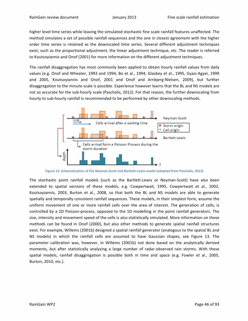
RainGain review document January 2013 Fine scale rainfall estimation
RainGain WP2 Page 46 of 93
higher level time series while leaving the simulated stochastic fine scale rainfall features unaffected. The method simulates a set of possible rainfall sequences and the one in closest agreement with the higher order time series is retained as the downscaled time series. Several different adjustment techniques exist, such as the proportional adjustment, the linear adjustment technique, etc. The reader is referred to Koutsoyiannis and Onof (2001) for more information on the different adjustment techniques.
The rainfall disaggregation has most commonly been applied to obtain hourly rainfall values from daily values (e.g. Onof and Wheater, 1993 and 1994, Bo et al., 1994, Glasbey et al., 1995, Gyasi-‐Agyei, 1999 and 2005, Koutsoyiannis and Onof, 2001 and Onof and Arnbjerg-‐Nielsen, 2009), but further disaggregation to the minute-‐scale is possible. Experience however learns that the BL and NS models are not so accurate for the sub-‐hourly scale (Paschalis, 2012). For that reason, the further downscaling from hourly to sub-‐hourly rainfall is recommended to be performed by other downscaling methods.
Figure 12: Schematisation of the Neyman-‐Scott and Bartlett-‐Lewis model (adapted from Paschalis, 2012)
The stochastic point rainfall models (such as the Bartlett-‐Lewis or Neyman-‐Scott) have also been extended to spatial versions of these models, e.g. Cowpertwait, 1995, Cowpertwait et al., 2002, Koutsoyiannis, 2003, Burton et al., 2008, so that both the BL and NS models are able to generate spatially and temporally consistent rainfall sequences. These models, in their simplest form, assume the uniform movement of one or more rainfall cells over the area of interest. The generation of cells, is controlled by a 2D Poisson-‐process, opposed to the 1D modelling in the point rainfall generators. The size, intensity and movement speed of the cells is also statistically simulated. More information on these methods can be found in Onof (2000), but also other methods to generate spatial rainfall structures exist. For example, Willems (2001b) designed a spatial rainfall generator (analogous to the spatial BL and NS models) in which the rainfall cells are assumed to have Gaussian shapes, see Figure 13. The parameter calibration was, however, in Willems (2001b) not done based on the analytically derived moments, but after statistically analyzing a large number of radar-‐observed rain storms. With these spatial models, rainfall disaggregation is possible both in time and space (e.g. Fowler et al., 2005, Burton, 2010, etc.).

RainGain review document January 2013 Fine scale rainfall estimation
RainGain WP2 Page 47 of 93
Figure 13: Rainfall distributed over Belgium and the Gaussian-‐shaped rainfall cells (after Willems, 2001b).
The point process theory based rainfall generators are also called stochastic rainfall generators. Stochastic rainfall generation, or as part of more general weather generation, can also be done by other methods, such as Markov chain approaches, which are discussed in the next section.
Cascade and multifractal methods Multifractals are a tool for the analysis and simulation of geophysical fields such as rainfall exhibiting extreme variability over wide range of spatio-‐temporal scales. They were initially introduced in the eighties following discussions on the scale-‐invariance properties of geophysical field (see Schertzer and Lovejoy, 2011 a recent review with an historical background). They rely on the assumption that rainfall is generated through a multiplicative cascade process that distributes intensity from large scale structures to small scale ones. In a discrete case a step of a cascade process consists in dividing a structure (a time step in for time series or a pixel for maps) into sub-‐structures and assigning to each sub-‐structure an intensity equal to the intensity of the parent structure multiplied by a random increment (see Figure 14a for an illustration).. The process is scale invariant in the sense that the way the structures are divided and the probability distribution of the random multiplicative increments are the same at each step of the cascade process. This concept is more than an ad hoc statistical tool fitted to rainfall fields since it is physically based in the sense that it is in agreement with the scale invariance properties of the Navier-‐Stokes equations governing atmospheric behaviour, which are assumed to be transmitted to the unknown equations for rainfall processes (Hubert, 2001). Various probability distributions have been suggested (see Schertzer and Lovejoy 1987, or Over and Gupta, 1996 for some famous examples) with this same underlying concept. Multifractal tools are commonly used our field (Gupta and Waymire, 1993; Harris et al., 1996; Marsan et al., 1996; Olsson and Niemczynowicz, 1996, de Lima and Grassman, 1999; Deidda, 2000 Pathirana and Herath, 2002; Biaou et al., 2003; Pathirana et al., 2003, Ferraris et al., 2003a and b; Macor et al., 2007; Royer et al., 2008; Nykanen, 2008; De Montera et al., 2009; Gires et al., 2012a and b, among others].

RainGain review document January 2013 Fine scale rainfall estimation
RainGain WP2 Page 48 of 93
Being intrinsically scale invariant these methods are capable of dealing with rainfall data at any (especially high in which we are interested here) spatial and temporal (minute-‐scale) resolution (e.g. Pathirana et al., 2003, Molnar and Burlando, 2005, Onof and Arnbjerg-‐Nielsen, 2009) and their validity is not limited to the resolution for which they were fitted.
Stochastic cascade models have been commonly used for downscaling rainfall fields (Biaou et al. 2003, Deidda, 2000; Ferraris et al., 2002; Olsson et al., 2001; Rebora et al., 2006a; Royer et al., 2008). Indeed they are very convenient for such a task since their structure is scale invariant. Downscaling is simply achieved by first estimating the relevant parameters of the underlying cascade process on the available range of scales (by performing a multifractal analysis on the data), and then stochastically continuing it to resolution higher than the observations’. Temporal, spatial and spatio-‐temporal downscaling can be implemented with the help of similar methodology. See Figure 14b for an illustration in 2D.
Figure 14: Rainfall downscaling a) Illustration of a cascade process in 1D and 2D (adapted from Gires, 2012),
b) an example of the spatial downscaling based on real data (adapted from Gires et al., 2012b)
Example from RainGain consortium: Multifractal cascade downscaling methods in practice:
Gires et al. (2012b, and 2012c) investigated the effect of the uncertainty due to the unknown small scale rainfall variability on a semi-‐distributed urban rainfall-‐runoff model. Unknown should be understood as occurring below the observation scale which was of 1 km in space and 5 min in time with the available C-‐band radar. In order to quantify the impact of the small scale variability, an ensemble set of realistic fine scale rainfall fields was generated based on the universal multifractal cascade approach (Schertzer and Lovejoy, 1987). These ensembles are then used as input for the urban rainfall runoff model and the in-‐sewer conduit flows were simulated. The variability among the simulated hydrographs is then estimated to quantify the uncertainty. This approach is applied on the Morée-‐Sausset catchment (a 3400 ha urban area situated in Seine-‐Saint-‐Denis, North-‐East of Paris, France) and the Cranbrook catchment (a 900ha urban area situated in the east of London, UK).
They implemented both spatial (2D) and spatio-‐temporal downscaling (3D). A schematization of the two approaches is shown in Figure 15. For this application only the more pedagogical discrete cascades were necessary, but it would be possible to implement similar techniques with continuous cascades (see

RainGain review document January 2013 Fine scale rainfall estimation
RainGain WP2 Page 49 of 93
Pecknold et al. 1993) for explanations on how to simulate them) which would avoid the rather unrealistic square structures visible on the downscaled field (Fig. 19). Comparison led to the conclusion that the 2D approach might overestimate the uncertainty, whereas the 3D approach gives more realistic results. They concluded that it is strongly recommended to use distributed (radar) rainfall in urban hydrology. Moreover, they encourage the use of X-‐band radar, which allows measuring rainfall at a higher resolution. The extra added value of radar measurements during summer is also endorsed by their results, especially for intense small scale convective events.
Figure 15: Illustration of the spatial (left) and spatio-‐temporal (right) downscaling techniques
Weather typing Within the weather typing approach, small scale rainfall features are linked to coarser scale weather patterns. From atmospheric conditions (pressure and temperature distributions, etc.), a specific set of so called ‘weather types’ (atmospheric circulation patterns with accompanying temperature distributions) can be categorized. They can be defined for every rain storm or time step, e.g. for every day or every one or several hours. Based on an historical dataset of events or time period where both coarse and fine-‐scale rainfall observations are available, for events or time steps where only the coarse scale rainfall data is available, the fine-‐scale rainfall values can be estimated by “copying” the most analogue event or time step from the historical dataset. The specific weather type of the event or time step, i.e. day, is used to define the day in that dataset with the most ‘analogue’ (large scale) atmospheric conditions. Instead of “copying” the fine-‐scale rainfall, one can also estimate the rainfall based on the downscaling relation for that analogue day. The measure of how analogue one day is to another can be defined based on several methods and can involve, besides the weather types also other factors, such as the season or the specific month, the temperature, the relative humidity, etc.
The weather types can be determined in several ways, which can be divided in two main groups. The first group, known as the subjective approach, tries to use prior knowledge and defines the weather types a priori, such as the Lamb weather types (Lamb, 1972) but several authors have adapted this

RainGain review document January 2013 Fine scale rainfall estimation
RainGain WP2 Page 50 of 93
method to be less subjective (e.g. the automated Lamb classification, Jenkinson and Collison, 1977). The second group of methods tries to cluster the days into specific subsets with high similarities; they do not assume prior weather types. Within this group, k-‐means clustering is widely used (e.g. Huth, 2001, Ullmann and Moron, 2008 and Ullmann and Monbaliu, 2009), but also other mechanisms are possible, such as neural networks, fuzzy logic, etc (see Vrac et al., 2007 or Mauran et al., 2010 for an overview of the different mechanisms).
Two weather typing methods (the automated Lamb weather typing and k-‐means clustering) have been applied for NW-‐Europe (for specific application of rainfall downscaling in Belgium) by Decloedt (2011), albeit for another purpose but the weather types are applicable to fine scale rainfall downscaling as well. A subset of the different weather types, both subjective (weather types West and North-‐West) and objective (cluster types Atlantic Ridge and Zonal) can be found in Figure 16, which shows the mean sea level pressure (SLP) maps for these specific weather or cluster types.
The method has been applied for rainfall downscaling by several authors (e.g. Goodess and Palutikof, 1998, Bellone et al., 2000, Vrac and Naveau, 2007, Willems and Vrac, 2011). Weather types have also been used for advancing stochastic weather or rainfall generators, by conditioning the parameters of the generator to weather types (e.g. Wilby et al., 1998 and 2002, Wilks, 1999, Wilks and Wilby, 1999, Bischoff and Vargas, 2003, Olsson et al., 2009, etc.).

RainGain review document January 2013 Fine scale rainfall estimation
RainGain WP2 Page 51 of 93
Figure 16: Mean SLP maps for a subset of different weather types for Belgium: A: through automated Lamb classification (weather types: West and North-‐West),
B: through k-‐means clustering (cluster types: Atlantic Ridge and Zonal) (after Decloedt, 2011)
Empirical transfer functions / Generalized linear models Empirical transfer functions relate large scale atmospheric information to small scale rainfall information. Within the class of empirical transfer functions, the generalized linear models (GLMs) are the most widely used methods. This can be done for each event or time step, or to relate fine scale rainfall statistics, e.g. probability distribution functions (PDFs), to the values of one or several associated predictors (also referred to as covariates).
The idea of transfer function models is to find relations between the fine scale rainfall information and suitable predictors and to estimate the fine scale rainfall information, based on the fitted relations and the predictors, for events that were not used in the deduction of the predictor relations. The linear regression model is the most popular one in this class. GLMs are an extension of this simple linear regression model, as they allow a wider set of fitted transfer functions and are better able to deal with data that is not normally distributed (Gill, 2000). More particularly, the GLM generalizes linear regression by allowing an arbitrary monotonic function of the dependent variables Y (called link function g) to vary linearly with the independent variables X: g(Y) = βX, where β are the regression parameters. This is different from the simple linear regression approach where the dependent variables themselves vary linearly: Y = βX. In this way, they also allow the magnitude of the variance of the dependent variable to be a function of the dependent variable, which is typically the case in rainfall downscaling applications.
The applications of GLMs for rainfall downscaling generally consist of a two phase approach (Figure 17), as is also the case for Markov Chain approaches. The first phase, the ‘Occurrence model’, consists of modelling the occurrence of dry and wet days. Most often a logistic regression is used for this. Hereafter, in the second phase, a PDF of the ‘Amounts model’ is used to predict the rainfall amount on the wet days.

RainGain review document January 2013 Fine scale rainfall estimation
RainGain WP2 Page 52 of 93
Figure 17: Schematization of the GLM downscaling method with the two phase approach,
consisting of the occurrence and the amounts models (adapted from Wang, 2012)
The GLM approach (e.g. Chandler and Wheater, 2002, Yang et al., 2005, Segond et al., 2006) has mainly been used for daily timescales but can be used to go further to the hourly or even minute-‐scale. The method was first developed for specific sites, but the spatial component is becoming more and more incorporated. Yang et al. (2005), for example, developed a method to generate rainfall series at multiple sites simultaneously. However, the GLM output quality strongly depends on the choice of the appropriate predictors (Wang, 2012).
Empirical transfer functions / Quantile mapping One option for the empirical transfer function approach is to relate the fine scale rainfall PDF directly to the coarse scale rainfall PDF. This can be done by quantile mapping (QM). The method has several synonyms in the literature: quantile matching, quantile-‐quantile (QQ) transformations, probability mapping, cumulative distribution matching, etc. These different names however stand for the same type of method, namely replacing the rainfall quantiles of the coarse scale PDF to the corresponding quantiles of the fine scale PDF. The method can also be used for distribution bias correction, e.g. correction of the downscaled rainfall distribution based on the observed rainfall distribution (e.g. Themeßl et al, 2011 and Gudmundsson et al., 2012). This method is an expansion of a simpler approach where only the distribution moments, e.g. the mean or the mean and the variance, are matched between the two distributions. With quantile mapping, the entire distribution is matched.
An example of a QQ-‐plot (quantile quantile plot) of observed (P0) and modeled (PM) precipitation together with the transformation function to map the quantiles together is shown in Figure 18, as well as the empirical cumulative distribution function (CDF) of the observed, modeled and transformed precipitation. Recent hydrological applications (e.g. Dettinger et al., 2004, Wood et al., 2004, Boé et al., 2007, Themeßl et al, 2011), mainly focus on statistical downscaling of climate model simulation results, but the method is well applicable to any coarse scale rainfall information.

RainGain review document January 2013 Fine scale rainfall estimation
RainGain WP2 Page 53 of 93
Figure 18: Example of the Quantile mapping method: left: a quantile quantile (QQ-‐) plot of observed (P0) and modeled (PM) precipitation and a transformation function (h) to map the quantiles together, right: the empirical cumulative distribution
function (CDF) of the observed modeled and transformed (h[PM]) precipitation (after Gudmmundsson et al., 2012).
Neural network models Another group of methods uses neural networks (NN, e.g. Gardner and Dorling, 1998) for the statistical downscaling of rainfall information. These neural networks, limited here to artificial NN, are black box models and they are good at linking nonlinear interactions between atmospheric processes at different scales (e.g. Giorgi and Mearns, 1991, Zorita and von Storch, 1999 and Olsson et al., 2004). A NN consists of a structure of interlinked nodes (the so called architecture of the network), where the architecture of the network can vary significantly in complexity. Each node or artificial neuron may have several inputs and one output. The output variable can be ‘trained’ based on the input variables and the expected output during the learning or training phase. After that, in the usage phase, the network will be able to predict autonomously the output variables based on the input and the learning procedures. In this prediction phase, the neuron looks for situations in the learning database matching or similar to the new situation and will select the output based on the output of that similar situation. Figure 19 represents the structure of a single neuron with its different inputs and output.
Figure 19: Artificial neural network schematization: a) representation of one single neuron and b) representation of a simple
feed-‐forward neural network architecture (adapted from Stergiou and Siganos, 1997)
Many different network architectures exist, ranging from simple feed-‐forward networks, see Figure 19b, to more complex systems with feedback loops. There is also the possibility to couple two NNs in series, where the first one determines whether the day is dry or wet and the second one determines the rainfall intensities during rainy days (e.g. Olsson et al., 2004). This is an analogue approach as applied in some of the GLM methods described above. For a more thorough discussion on neural networks, the reader is referred to the literature (books by e.g. Smith, 1993 and Bishop, 1995 or review papers by e.g.

RainGain review document January 2013 Fine scale rainfall estimation
RainGain WP2 Page 54 of 93
Maier and Dandy, 2000, among others). Applications of neural networks in hydrology include Hewitson and Crane (1992), Cavazos (1997), Crane and Hewitson (1998), Wilby et al. (1998), Olsson et al. (2001 and 2004), Schoof and Pryor (2001), Cannon and Whitfield (2002), Tatli et al., (2004), Coulibaly et al., (2005), among others.
Statistical methods to relate coarse-‐scale rainfall statistics to fine-‐scale rainfall statistics The weather typing, neural network and empirical transfer function based methods, including quantile mapping, as explained in the previous section, relate large scale atmospheric information to small scale rainfall information. These methods were explained to be applied on an event or time step, e.g. day to day, basis. They can equally well be applied to downscale rainfall statistics, such as probability distributions or moments, quantiles or percentiles, extreme value distributions or rainfall intensities for given return periods or recurrence intervals, etc.
Markov chain based disaggregation method A Markov chain model simulates the state of a certain variable based on the previous states of that variable and the transition probability matrix. The latter matrix contains the probabilities that a given current state of the modelled variable changes to the same or another predefined state. The number of previous states incorporated in the model defines the complexity, which may vary from a ‘first order’ Markov chain where only the last state is incorporated, to far more complex models. In our case the modelled variable is the rainfall volume or intensity, but in the literature several other variables are also modelled based on this approach (according to Salas et al., 2003: temperature, water storage in reservoirs, stream flow, among others).
For example, imagine the simple first order Markov chain with two states, being wet (raining) and dry, shown in Figure 20. In this case, the transition probability matrix is a two by two matrix as shown in equation VI-‐1, where P(x|y) denotes the probability that, given state y, the following state will be x. The rainfall intensity on the wet days is then generated based on random sampling from rainfall probability distributions.
( ) ( )( ) ( )
P dry dry P wet dry
P dry wet P wet wet
⎡ ⎤⎢ ⎥⎢ ⎥⎣ ⎦
VI-‐1
Figure 20: Schematization of a first order two state Markov chain (adapted from Hocaoğlu, 2011)
The number of different (non-‐zero) rainfall states can also be higher than one. For example, Giambelluca and Oki (1987) used 10 (9 non-‐zero) rainfall states. The first Markov chain based approaches were

RainGain review document January 2013 Fine scale rainfall estimation
RainGain WP2 Page 55 of 93
designed for single site estimation (e.g. Giambelluca and Oki, 1987 and Rajagopalan et al., 1996), but spatially distributed versions also exist (e.g. Mackay et al., 2001 and Allcorft and Glasbey, 2003).
The order-‐estimation problem has been discussed by several authors, e.g. Chin (1977), Katz (1981), Zhao et al. (2001) and Baigorri et al. (2012), among others. The parameters of the Markov chain can also vary in time, based on diurnal or seasonal variations, or atmospheric indices such as different atmospheric circulation patterns or even based on a trend function. These types of Markov chains are called ‘non-‐homogeneous’ Markov models (NHMMs) (e.g. Mimikou, 1983; Rajagopalan et al., 1996; Hughes et al., 1999 and Bellone, 2000).
A Markov chain can incorporate a so called ‘hidden’ parameter, a parameter of which “we do not assume an explicit, definitive observation of the state sequence, although the Markovian structure of the state sequence is strictly implied” (Hughes et al., 1999). These methods mostly use the weather state as hidden parameter and are known as Hidden Markov Models (HMMs) (e.g. Zucchini and Guttorp, 1991; Hughes et al., 1999; Bellone et al., 2000 and Kirschner, 2005). A HMM can also be non-‐homogeneous, resulting in a NHHMM (non-‐homogeneous HMM) (e.g. Hughes et al., 1999 and Bellone, 2000).
Scaling relations Many (geo-‐) physical processes and phenomena, including rainfall, show scaling properties over a wide range of spatio -‐ temporal scales. Indeed, for rainfall, relations can be found between fine-‐scale rainfall characteristics and predictors at coarser scales (both temporal and spatial). These scaling properties of rainfall are also investigated within the multifractal framework (see before). They are also more generally used within a group of rainfall downscaling methods, as they make it possible to scale not only the rainfall moments, but also its entire distribution.
The scaling properties of rainfall also become visible when analyzing IDF-‐relationships. As mentioned before, the IDF-‐relations describe the relationship between the mean rainfall intensity with the duration over which the precipitation is averaged and this for different return periods. The duration is also called the ‘aggregation level’. The return period is the inverse of the frequency of occurrence. An example of a set of IDF curves for different return periods is shown in Figure 21 (after Willems, 2000).

RainGain review document January 2013 Fine scale rainfall estimation
RainGain WP2 Page 56 of 93
Figure 21: IDF-‐relationships for return periods of 27, 9, 2.7 and 1 years;
comparison of calibrated IDF-‐relationships (full lines) with observations (source: Willems, 2000)
With the IDF relations, the rainfall properties are investigated over a range of aggregation levels. Based on the relation of the rainfall distribution parameters with the aggregation level, the scaling properties and relations can be determined, as the aggregation level can be seen as the time variable in scaling theory terminology. According to Willems (2000), for Belgium, these distribution parameters have a power law relation with the aggregation-‐level, as represented in equation VI-‐2.
baDβ = VI-‐2
The existence of these scaling relations means that if the rainfall parameter values are known for one certain aggregation level, they are also known for all other aggregation levels only by applying a scaling factor, as shown in equation VI-‐3. Both equations VI-‐2 and VI-‐3 give the example of the parameter β, where λ is the scale factor and b the scaling exponent. The scaling exponent equals the linear slope of the relationship between β and D in a double logarithmic plot. The scaling property of equation VI-‐3 is also called `scale invariance'.
bλβ λ β= VI-‐3
With these scaling relations, for example, 10 minute rainfall information can be derived based on hourly data, as with the scaling parameters, the IDF determines the rainfall distribution for any aggregation level. This type of downscaling is however restricted to the temporal aspect (e.g. Menabde et al., 1999, Borga et al., 2005, Bougadis and Adamowski, 2006, Nhat et al., 2007).
The spatial aspect can be integrated, based on areal rainfall IDF relations. These areal IDFs can be based on spatially distributed rainfall information (e.g. radar data), from which the scaling properties of the rainfall can be derived and applied to support the downscaling of the rainfall PDFs to the desired (finer) scales. Sivapalan and Bloeschl (1998) implemented a method based on the spatial correlation structure of rainfall to construct IDF curves.

RainGain review document January 2013 Fine scale rainfall estimation
RainGain WP2 Page 57 of 93
Example from RainGain consortium: Intensity-‐Duration-‐Frequency relations and scaling properties in practice:
To derive IDF-‐relationships, the proper type of distribution is selected first by an extreme value analysis and the distribution parameters are calibrated for a given range of aggregation-‐levels. Afterwards, the relationships between model parameters and aggregation-‐level are analyzed. The model parameter values are eventually modified a little, while still being acceptable, to derive smooth relationships. The parameter/aggregation-‐level relationships, together with the analytical description of the extreme value distribution, then comprise the IDF-‐relationships.
As an example for Belgium, the scaling properties of the IDF relation parameters will be discussed hereafter, based on Willems, 2000 and Willems, 2001b. In these works, he defined a ‘two-‐component exponential distribution’ according to equation VI-‐4, where Ga(x) and Gb(x) are two different exponential distribution functions. These two different distributions represent two different rainfall regimes: storms with convective rain cells (summer storms) and storms with many spatially clustered rain cells (cyclonic and frontal winter storms). The parameter pa represents the proportion of the summer storms and the parameter xt represents the threshold value for the rainfall intensity (above which the exponential distribution is fitted).
( ) ( ) ( ) ( )
( )
( )
1
1 exp
1 exp
a a a b
ta
a
tb
b
G x p G x p G x
x xG x
x xG x
β
β
= + −
⎛ ⎞−= − −⎜ ⎟
⎝ ⎠
⎛ ⎞−= − −⎜ ⎟
⎝ ⎠
VI-‐4
These distribution parameters can however also be a function of the aggregation level. When examining this in a log-‐log plot, as shown in Figure 22, it becomes evident that there are indeed relations between the parameters and the aggregation level.
Figure 22: Scaling properties of the parameters of the two-‐component exponential distribution (after Willems, 2000)

RainGain review document January 2013 Fine scale rainfall estimation
RainGain WP2 Page 58 of 93
These relations can be approximated by the ones shown in equation VI-‐5 and they are a representation of the scaling properties of the rainfall parameters with the aggregation level.
[ ]( ) [ ]( )[ ]( ) [ ]( )
( ) [ ]( )
log mm/h 0.05 0.58log days
log mm/h 0.55 0.58log days
log 1.35 0.58log days
a
b
a
D
D
p D
β
β
= − −
= − −
= − −
VI-‐5
In the Belgian case, as can be seen from equation VI-‐5, the scaling exponent b (equation VI-‐3) is the same for all parameters, namely 0,58; indicating that, after scaling of the rainfall intensities, the same exponential distribution is found for all aggregation-‐levels, as shown in equation VI-‐6. This means that, if all rainfall intensities are scaled with a factor λb, also the specific rainfall intensity (the threshold level xt) and the mean rainfall intensity exceeding the threshold (the scale parameter β) will be scaled with the same factor.
( ) ( )
( ) ( ), ,
, ,
ba D a D
bb D b D
G x G x
G x G x
λ
λ
λ
λ
=
= VI-‐6
Areal correction factors A popular method from the water engineering field that in fact also relates fine to coarse scale rainfall statistics is the areal correction factor (ACF, US Weather Bureau, NSSP, 1961, UK National Environmental Research Council, NERC, 1975). This factor represents the mean ratio of the spatially averaged rainfall volume over the point rainfall volume.
Two types of ACFs exist: for individual historical storms (storm-‐centered type) and for design rainfall for given return periods (fixed-‐area type), e.g. Willems and Berlamont, 2002. The more general term ‘areal correction factor’ or ‘areal correction coefficient’ was suggested by Vaes et al. (2005), as they discovered that for urban drainage applications, the areal reduction factor (ARF) may also reflect an increase instead of a reduction. Willems and Berlamont (2002) developed both types of ARFs for Belgium based on a large number of simulations with the stochastic spatial rainfall generator for Belgium (Willems, 2001b). An example of the first type of ACF is shown in Figure 23, where the ACF is shown for an aggregation level of 10 minutes and as a function of the size of the catchment area and the measured point rainfall intensity (after Vaes et al., 2005). They found relationships between the ACF and (i) the catchment area, (ii) the rainstorm volume, (iii) the distance between the catchment centre and the location at which the point rainfall is considered, and (iv) the peak intensity (Willems and Berlamont, 2002).
For a review on areal reduction factors, the reader is referred to Srikanthan (1995) or more recently, Svensson and Jones (2010) and Willems et al. (2012). Applications of the areal reduction factors to rainfall estimation include Lorente and Redafio (1990), Asquith (1999), Allen and DeGaetano (2005), among others. The use of radar data within the ARF framework has also been proposed and tested (e.g.

RainGain review document January 2013 Fine scale rainfall estimation
RainGain WP2 Page 59 of 93
Stewart, 1989, Durrans et al., 2002, Lombardo et al., 2006 and Overeem et al., 2010) and shows good results compared to the other ARF methods. It is clear that also the scaling properties of rainfall, as discussed in the previous sections, might be very helpful in deriving ARFs.
Figure 23: Median values for the areal correction coefficients (type I) for an aggregation level of 10min as a function of the measured rainfall intensity at the central point location (after Vaes et al., 2005)
iii. Comparison methods Before adjusting and integrating the radar measurements to and with the rain gauge measurements, it is important to have an idea of the performance of the two compared to each other. This comparison is done as a check for the calibration and correction procedures of the radar (the consistency check) but it could also be part of the quality control on the radar and gauge measurements. As mentioned in the previous section, the radar and gauges do not actually measure the same types of rainfall. This means that there are several approaches for the comparison, which either account for the differences and try to compensate or accept the differences and try to incorporate them into the comparison.
These methods will be discussed hereafter, but they can all be applied on different timescales. The rainfall measurements can be compared on an event basis by firstly selecting from the time series the different rain events or storms and comparing one or more of the rain event characteristics such as the total rainfall amount, the peak intensity, the averaged rainfall intensity during the event, etc. The comparison could however also be done over a longer period of time, e.g. monthly statistics, seasonally, yearly, even for longer time periods. The comparison could also be based on probability distributions of the rainfall intensities (possible for different averaging times) or summarized in the form of IDF (intensity -‐ duration – frequency) relations (for an example of a set of IDF curves for different return periods, the reader is referred to Figure 21 on p56, after Willems, 2000).
Methods accounting for the differences between the measurements
In this approach, the differences between the two types of measurements are accounted for and the spatial scale of one of the two is adapted towards the scale of the other. There are two possibilities,

RainGain review document January 2013 Fine scale rainfall estimation
RainGain WP2 Page 60 of 93
either to downscale the radar results to point scale or to spatially interpolate the point measurements (e.g. Sinclair and Pegram, 2005). The downscaling of the radar results is a rather uncommon way of comparing the measurements. Section ii of this chapter discussed the different downscaling methods, an example is given in the box below.
Example from the RainGain consortium: Downscaling radar fields to revisit standard comparison tools between radar and point measurement
Gires et al. (2013) suggest to use downscaling in order to bridge the gap between the observation scale of weather radar and point measurements, but also to take this gap into account when using the standard comparison tools (such as the temporal evolution of the rainfall rate or the cumulative rainfall depth, the normalized bias, the RMSE, the correlation coefficient, the Nash-‐Sutcliffe coefficient, etcetera …). The analysis is performed on 4 rainfall events that occurred in the Paris area between 2009 and 2011. The radar data comes from the Météo-‐France mosaic (with a resolution of 1 km in space and 5 min in time), and the rain gauge data (with a resolution of few tens of cm in space and 5 min in time) comes from the operational network of 26 rain gauges of the Direction Eau et Assaisnissement of Conseil general (local authority in charge of urban drainage) of the Seine-‐Saint-‐Denis County (North-‐East of Paris, France).
More precisely Gires et al. downscale the radar data down to the resolution of the rain gauges. This is achieved by implementing 7 steps of spatio-‐temporal Universal Multifractals cascades on the radar data and then re-‐aggregating the obtained field in time. This process enables to generate realistic output of 2187 x 2187 “virtual point measurement” devices located within each radar pixel. The variability among these “virtual points” represents the one that would naturally be expected simply because of small scale rainfall variability.
Then in order to quantify the impact of small scale rainfall variability on the standard comparison scores (parameters such as the RMSE, normalised bias etcetera) a “virtual point measurement” is randomly selected for each radar pixel and the corresponding scores are computed. To generate a distribution of possible values for each score, 1000 sets of 26 virtual rain gauges locations (one per radar pixel) are tested. Figure 24 displays results for RMSE with a 15 minutes resolution (the results for other scores and temporal resolution are visible in Gires et al. 2013).
It appears that this influence is twofold. First the target values of the scores are not the optimum ones because rainfall variability “naturally” worsens them. This worsening which is neglected in published comparison is significant. Second because of the random position of the point measurements within a radar pixel there is an expected uncertainty on a computed score reflected in Figure 24 a by the width of the distribution. When rainfall rate or cumulative depth temporal evolution are compared the authors also recommend to display the uncertainty bounds (i.e. the quantiles of the “virtual point measurements”) associated with the radar data at the point measurement resolution to have immediate insight into the effect of small scale rainfall variability. An example is provided Figure 24 b and c.

RainGain review document January 2013 Fine scale rainfall estimation
RainGain WP2 Page 61 of 93
Figure 24: (a) Histograms the RMSE scores with a 15 min time step computed for the 1000 samples of possible combinations of virtual rain gauges for the 4 studied event (b) Rain rate temporal evolution for 14 July 2010 for a radar pixel in Seine-‐Saint-‐Denis: rain gauge (dash), radar (solid), and uncertainty range of the radar measurement at the rain gauge scale. (c) As (b) for temporal evolution of cumulative depth. (Adapted from Gires et al. 2013)
Through spatial interpolation or upscaling of the point rainfall measurements at ground-‐level, it is possible to form rainfall data at radar scale before comparing the two sources of rainfall information. There are several principles available, ranging from very straightforward to more complex methods. The interpolation procedures such as the isohyetal method or ordinary kriging will be discussed, but also other methods, such as the Thiessen method, fall within this category.
The isohyetal method (Linsley et al., 1949 and Jain and Singh, 2005) draws lines of equal rainfall depth or intensity based on the point measurements of the gauges. The method also imposes several restraints on the form of the isohyets. Figure 25 B shows an example result of the isohyetal method.
The Thiessen polygon method (Thiessen and Alter, 1911, Linsley et al., 1949, Brassel and Reif, 1979 and WMO, 1986) assigns to each point in space the value of the closest rain gauge, without any interpolation or distance factor. Figure 25 shows an example of a drainage basin with rain gauge measurements and the application of the isohyetal (B) and the Thiessen methods (C).
Figure 25: Rainfall interpolation methods based on gauges: A: a drainage basin with rain gauges (their position is marked by their respective measurement values), B: the spatial rainfall distribution based on the isohyetal method and C: the spatial
rainfall distribution based on the Thiessen method (adapted from Fetter, 1994)
The inverse distance weighting procedure (IDW, Burrough and McDonnell, 1998, Miras-‐Avalos et al., 2007 and Lu and Wong, 2008) is an interpolation method that calculates the rainfall value at a given

RainGain review document January 2013 Fine scale rainfall estimation
RainGain WP2 Page 62 of 93
point from measurements in the proximity of that point. The weights assigned to these measurements are inversely related to their distance to the point.
The ordinary kriging method (KRI) is a geostatistical method using only rain gauge data. The original method (Goovaerts, 1997) is a spatial interpolation of a random field of observations at several different locations (in our case, rain gauges or other point information rainfall sources). The rainfall estimation (U0 in equation VI-‐7) at any location is a weighted linear combination of the observations of the nearby gauges, where the weights (lambda) are computed by solving a set of linear equations (size equal to the available number of gauges) to obtain the best linear unbiased estimator assuming a constant unknown mean across the field. This is done based on a variogram that characterises the spatial variability of the estimated rainfall field (based only on the gauges). The ordinary kriging method can be used to compare the spatially interpolated gauge rainfall fields with the radar rainfall fields, but also to assess the added value of the radar measurements, when comparing the results from the ordinary kriging method to methods using radar data.
01
N
i ii
U Gλ=
=∑ VI-‐7
Methods incorporating the differences between the measurements
In this approach, the differences between the two types of rainfall data are accepted and the comparison will be less strict as they cannot be identical (nor should they be). The closeness of the measurements however gives a general idea of the overall performance of the two. It is also an option to calculate (or estimate if calculation is not possible) the uncertainty on each measurement and to use not only the exact values in the assessment of the closeness of the measurements, but also the uncertainty margins of each of the measurements. This allows for a more comprehensive comparison.
iv. Adjustment or integration principles and methods Several adjustment or integration principles and methods exist. They mostly acknowledge that the radar observes the spatial distribution of the rainfall fields correctly, but that rain gauges (or other point measurements such as disdrometers) have a higher accuracy at the point scale. A summary of the different approaches is given and each method is discussed thereafter. An extensive review report on gauge adjustment methods can be found in Gjertsen et al. (2003). This COST 717 report also discusses the operational use of these methods (in Europe).
Adjustment methods
The adjustment methods aim to correct one of the sources of rainfall information, the radar estimates, based on the other, the rain gauge measurements. For this adjustment, several different methods exist and are discussed hereafter.
Mean field bias correction The Mean Field Bias correction method (MFB) assumes that the radar estimates are affected by a uniform multiplicative error. The adjustment factor CMFB is given by a comparison with the rain gauges as determined by equation VI-‐8, where N is the number of valid radar-‐gauge pairs, Gi and Ri are the gauge

RainGain review document January 2013 Fine scale rainfall estimation
RainGain WP2 Page 63 of 93
and radar values associated with gauge i. The offset between the gauges and the radar can be due to an offset in the electronic calibration or an offset in the Z-‐R relation used for the rainfall estimation. This method is one of the simpler methods and has been applied by Fulton et al. (1998), Harrison et al. (2000), Borga et al. (2002), Holleman (2007), among others.
1 1
N N
MFB i ii i
C G R= =
=∑ ∑ VI-‐8
Range-‐dependent adjustment The range dependent adjustment (RDA) procedure is a form of bias adjustment. However, the bias is allowed to be a function of the distance from the radar. The range dependence of the bias can be explained by beam broadening and attenuation effects. The distance weighing can be done in several ways, e.g. Goudenhoofdt and Delobbe (2009) used a second order polynomial regression line (in the log scale) fitted by least squares minimization. For more information, see Michelson et al. (2000) or Goudenhoofdt and Delobbe (2009), among others.
Brandes correction The Brandes correction method (BRA) was proposed by Brandes (1975) and comprises of a correction factor calculated based on an interpolated field of correction factors calculated at each rain gauge. This is thus a spatially distributed correction method, opposed to the MFB method. Equation VI-‐9 shows this principle, where w is the weighting factor, d is the distance from the grid point to the nearest gauge and k is a smoothing parameter. This factor k can be chosen and optimized, for example, Goudenhoofdt and Delobbe (2009) used 𝑘 = (2𝛿)!!, where delta is the gauge density of the network. The method is thus a spatial method and it follows the Barnes objective analysis scheme (using a negative exponential weighting function).
( ) 2
1
1
where exp
N
i i ii i
BRA iN
ii
w G RdC wkw
=
=
−= =∑
∑ VI-‐9
Several different kriging methods exist, such as kriging with radar based error correction, kriging with external drift, etc. These methods will be discussed hereafter.
Kriging with radar-‐based error correction The kriging method with radar-‐based error correction (KRE) method is an expansion of the ordinary kriging method, as it uses radar data to correct the errors associated with its estimates. The ordinary kriging method is used, but this time based on the radar data instead of the gauges (only the radar data from the gauge sites are used). This rainfall field is subtracted from the original radar field to obtain the error field, which is added to the gauge based kriging field. The method thus adds the spatial variability of the radar measurements to the gauge based kriging field.
Kriging with external drift The kriging with external drift (KED) method is similar to the ordinary kriging method, except that the rainfall estimates are now a function of the radar estimates instead of the gauge information, with

RainGain review document January 2013 Fine scale rainfall estimation
RainGain WP2 Page 64 of 93
additional constraints. These constraints take the form of equation VI-‐10, where Ri are the radar values at the gauge points, lambda are the weights and R0 is the estimate at a chosen location. The weights for each specific location are calculated by solving the kriging equations with the additional constraints. More information can be found in Wackernagel (2003). KED is one of the most widely used kriging methods.
01
N
i ii
R Rλ=
=∑ VI-‐10
Regression kriging Regression kriging is, like the other kriging methods, a spatial interpolation technique. It combines a regression model with the simple kriging of the residuals of this regression model. The regression of the dependent variable is based on a secondary variable (which could be any variable, but this is most commonly a land surface parameter such as the elevation or others), in order to remove the trend between the two, before using the residuals of this detrending for simple kriging. Hengl et al. (2007) used the term regression kriging, while Goovaerts (1999) used ‘kriging after detrending’. The approach of the methods is however identical.
Integration methods
There are, however, also methods which integrate the radar and gauge measurements and use the combination of the two to obtain the best possible rainfall estimates. These methods, such as co-‐kriging and Kalman filtering, are mostly more complex than the previous ones.
Co-‐kriging Co-‐kriging uses both rain gauge and radar data in a procedure similar to the ordinary kriging method. It was developed for regions with a very limited number of gauges, so very limited information about the spatial variability of the rainfall fields was captured by those gauges. The second variable, the radar could thus help recover the variability and improve the quality of the rainfall estimates. The method is described by equation VI-‐11, where GI are the gauge measurements and RK the radar measurements. Lambda and gamma are the respective weights of the gauge and radar measurements, and are computed by resolving the covariance and cross-‐covariance matrices. More information can be found in Krajewski, (1987), Creutin et al. (1988) and Sun et al. (2000), among others. The number of radar grid points (M) is mostly at least an order of magnitude higher than the number of gauges (N).
1 1
N M
i i k ki k
R G Rλ γ= =
= +∑ ∑ VI-‐11
Kalman filter This filter implements an iterative process designed by Kalman (1960). It is widely applicable to several modeling applications. The Kalman filter method can be applied to remove time varying field bias. In general, the Kalman filter consists of two types of equations: state-‐space model or system equations and observation equations. The general form of the problem the Kalman filter addresses is shown in equation VI-‐12, where the matrix A represents the link between the previous values of the state variables (xk-‐1) with their current value (xk), and the matrix B represents the influence of the (optional)

RainGain review document January 2013 Fine scale rainfall estimation
RainGain WP2 Page 65 of 93
control value or control input uk-‐1. H represents the relation between the state variables xk and the measurements zk. The random variables wk-‐1 and vk represent respectively the process and measurement noise. In our applications, the state variables are the QPE estimates and the measurements are the radar and rain gauge measurements, optionally extended with other sources of rainfall information.
1 1 1k k k k
k k k
x Ax Bu wz Hx v
− − −= + +
= + VI-‐12
The Kalman filter considers an iterative two-‐step procedure. As an initialization, the current state of the modeled variables is estimated. In step 1, the prediction or time update step, the state variables are projected to the next time step by means of equation VI-‐13. The predicted new state is called the ‘prior estimate’, as this estimate will be corrected when more recent measurements become available. The error covariance matrix P, which contains the error variances and covariances of/between the prior estimates of the different state variables, is also projected to the next time step.
1 1
1
ˆ ˆk kkT
kk
x Ax Bu
P AP A Q− −
−
= +
= + VI-‐13
Hereafter in step 2, the correction or measurement update step, the prior estimate is corrected based on the current measurements z using a weighting method, with higher weights for estimates with higher accuracy. This weighting method uses the Kalman Gain K. The corrected estimate is known as the ‘posterior estimate’. The error covariance matrix P is also updated. The mathematical equations are
shown in equation VI-‐14, where ˆkx represents the prior estimates of the state variables and ˆkx the
posterior state variables’ estimates, K is the Kalman Gain or blending factor, Q is the process noise covariance matrix and R the measurement noise covariance matrix.
( )( )
( )
1
ˆ ˆ ˆ
T Tk k k
k k kk k
k k k
K P H HP H R
x x K z Hx
P I K H P
−= +
= + −
= −
VI-‐14
Because of the algorithm's recursive nature, it can run in real time using only the present input measurements and the previously calculated state; no additional past information is required. Through the covariance matrices Q and R, the Kalman filter can account for the model and observation errors (see also section v of this chapter on uncertainty analysis).
More information on the Kalman filter method can be found in Maybeck (1979, Chapter 1), Sorenson (1970) or Welch and Bishop (2006). The method has been applied for urban rainfall estimation before by Ahnert (1986), Smith and Krajewski (1991), Anagnostou et al. (1998), Seo et al. (1999), Todini (2001), Dinku et al. (2002), Seo and Breidenbach (2002), Anagnostou and Morales (2002), Chumchean (2004) and Chumchean et al. (2006), among others.
Example: Kalman filter in practice:

RainGain review document January 2013 Fine scale rainfall estimation
RainGain WP2 Page 66 of 93
Chumchean et al. (2006) proposed a real time procedure for the integration of radar error correction and bias adjustment in the radar rainfall estimation procedure. The error correction strategies in the paper correct errors in the reflectivity measurements and the reflectivity conversion (Z–R). For the mean field bias removal, the Kalman filter was applied to the radar data. For the validation of their approach, a 7-‐month record of radar and rain gauge rainfall for Sydney, Australia, were used. Data from a C-‐band Kurnell-‐radar were used together with point rainfall information for 173 rain gauges in the proximity of the radar.
They conclude that, as shown in Figure 26, after application of the bias-‐adjustment based on the Kalman filter, the best possible radar-‐rainfall estimates (lowest RMSE) were achieved for all cases investigated in their research. This conclusion, however, only holds when the other error sources are accounted for. They indeed conclude that, while the effect of the error correction strategies is small compared to the bias correction, it is a very important step in the radar processing chain. Without proper error correction, the bias corrected results could even be worse than the original estimates.
Figure 26: Validation of the RMSE for radar based rainfall QPEs for a different number of calibrated gauges and different error correction strategies with a) no bias adjustment and b) Kalman filtering. Note: “GHNBO” denotes correction of ground clutter, hail, and noise and range-‐dependent bias resulting from bright band and different observation altitude, “SC” denotes correction of range-‐dependent bias resulting from increases in observation volume (scaling correction) and “ZR” denotes correcting for variation of Z–R relationship for convective and stratiform rainfall (storm classification) (Adapted from Chumchean et al., 2006).
Comparison of different methods
Several researchers compared the different methods for their own radar and rain gauge data. An overview will be given, but no overall conclusions could be made, since not all studies compare the same techniques and the comparison also depends on site specific radar and rain gauge characteristics. Only a limited number of studies have focused on the impact of these characteristics, such as for example the density of the gauge network (e.g. Sokol, 2003 and Chumchean et al., 2006).

RainGain review document January 2013 Fine scale rainfall estimation
RainGain WP2 Page 67 of 93
Most studies (e.g. Creutin and Obled, 1982, and Goovaerts, 2000, among others) show that for low density rain gauge networks, the geostatistical interpolation methods (KED, KRE, Co-‐kriging) outperform the other methods that ignore the spatial patterns of the rainfall fields, such as MFB or others. For high density rain gauge networks, the added value of KED and KRE over ordinary kriging is rather low, especially for frontal or long-‐lasting spatial storms in the winter season (Goudenhoofdt and Delobbe, 2009). For convective storms, which frequently occur in the summer season, the added value of the radar estimates is evident. Hevesi et al. (1992a and b) found that the co-‐kriging method performed best for their case study. Other researchers (e.g. Haberlandt, 2006, Schuurmans et al., 2007, Goudenhoofdt and Delobbe, 2009, Velasco-‐Forero et al., 2009) identified the kriging method KED to be the best estimator (the KRE method gave mostly similar results as the KED method).
The Kalman filter approach generally also gives good results, but comparison to the kriging methods is rather rare. Most studies only compare but a small number of methods and mostly for short time periods, so the conclusions are not generally applicable to any given situation.
Example from RainGain consortium: Adjustment methods in practice:
Shrestha et al. (2012) investigated the accuracy of rainfall estimates from both C-‐ and X-‐band weather radars and their application for stream flow simulation. They also tested several adjustment procedures (Range dependent adjustment, Mean field bias correction and Brandes spatial adjustment), which were applied to the raw radar measurements and used supplementary rainfall information from a network of 12 rain gauges. The C-‐band radar at Wideumont and the X-‐band LAWR-‐CR radar at Leuven, are used. The C-‐band radar is operated by the Royal Meteorological Institute of Belgium (RMI), while the X-‐band radar is operated jointly by Aquafin and KU Leuven (Goormans and Willems, 2012).
Their results showed that the raw radar estimates could be greatly improved by all the adjustment procedures. For the different adjustment methods, the Brandes method slightly outperformed the others (MBF and RDA for the X-‐band radar and MFB, for the C-‐band radar), as shown in Figure 27. The gauge-‐radar residuals however remain quite large, even after the adjustments.
Figure 27: Comparison of the performance of the radar adjustment procedures: a) LAWR-‐CR X-‐band and b) RMI C-‐band,
comparison of the statistical indicators for summer (adapted from Shresta et al., 2012)

RainGain review document January 2013 Fine scale rainfall estimation
RainGain WP2 Page 68 of 93
Goudenhoofdt and Delobbe (2009) investigated a set of adjustment methods for the C-‐band radar of the RMI (including MFB, RDA and BRA, but also kriging based methods) and found the kriging methods KRE and KED to be the best methods, as can be seen in Figure 28. Their research supports the conclusion of Shrestha et al. (2012) that the Brandes method outperforms the MFB and RDA approaches.
Figure 28: Comparison of the performance of the radar adjustment procedures (after Goudenhoofdt and Delobbe, 2009)
Shrestha et al. (2012) also concluded that the adjusted X-‐band radar measurements are better estimates than the corresponding C-‐band measurements, as can be seen in Table 2. This table shows the different statistical indicators for the summer and winter periods after the adjustments on the LAWR-‐CR (X-‐band) and RMI (C-‐band) radar based estimates. Further investigation showed that the rain gauges and radars could simulate the spatially more uniform winter storms with almost the same accuracy. The results are different for summer events, where the added value of the radar data becomes more evident.
Table 2: Different statistical indicators for the summer and winter periods after the adjustments on the LAWR-‐CR X-‐band and RMI C-‐band radar based estimates (after Shrestha et al., 2012).
v. Incorporating uncertainties when merging rainfall data When rainfall measurements with different resolution are merged together to obtain best rainfall estimates, question is whether the finer resolution data should be upscaled to the coarser scale data, or vice versa. This of course depends on the application. It indeed depends on the scale at which the rainfall data is required. For urban drainage applications, fine scale rainfall estimates are required; hence downscaling will be more appropriate than interpolation or upscaling.

RainGain review document January 2013 Fine scale rainfall estimation
RainGain WP2 Page 69 of 93
The different possible approaches for the merging process have been discussed already in the previous section of this chapter. That section also explained that the differences in accuracy between the different types of rainfall data can be accounted for. In addition to this, the conditional merging approach was explained earlier in this chapter (see Interpolation and upscaling methods, p43). This section explains how the merging can be done taking the uncertainties in the different rainfall data into account. Use is made of methods that have been discussed before, e.g. kriging methods or Kalman filtering techniques, but more specific methods exist as well.
Kalman filter
The Kalman filtering technique has the ability to integrate different sources of rainfall information in one procedure, while at the same time taking the uncertainty in account. The method was explained in detail in section iv of this chapter. The Kalman filter propagates the error information explicitly through dynamic equations based on the state error covariance matrix. It is also possible to use an ensemble of model trajectories in order to estimate the error covariances (Evensen, 1994). This technique is known as the ensemble Kalman filter (Reichle et al., 2002).
Kriging methods
The kriging based methods such as kriging with external drift (KED) and kriging with radar-‐based error correction (KRE), as well as the Co-‐kriging approach (all described in chapter VI) are widely used to merge radar and rain gauge rainfall information. They not only provide a merged rainfall field, but also an uncertainty assessment through the so called kriging standard deviation (by theoretical interpolation, Moulin et al., 2009). The uncertainty on these error estimates however can be rather high (e.g. Schiemann et al., 2010); which would mean that in this case other ways of uncertainty assessment are preferable. The quality of the kriging methods as merging tools is extensively documented in the literature, as shown in section iv of this chapter.
Radar QPE methods incorporating error/uncertainty assessment
The goal of the merging is to derive quantitative precipitation estimates (QPE). Several QPE methods have specially been designed to incorporate the error structure of the radar based rainfall estimates. These methods (e.g. Habib et al., 2004, Ciach et al., 2007, Germann et al., 2009, Kirstetter et al., 2010) generally have a three step approach: first, a thorough quality control of all rainfall information sources, including rejection of suspicious or uncertain sources; in a second step, some form of ‘reference rainfall’ is deduced after which, in the last step, a statistical error model is set up. The reference rainfall is mostly a kriged rainfall field based on rain gauge information, but the specifics of each step depend on the author. With this approach, uncertainty can be reduced and a set of possible ensembles generated, which helps to improve the radar QPEs.
Habib et al. (2004) use an observational-‐based empirical approach called the ‘conditional distribution transformation’ (CDT) to analyze different characteristics of the total radar-‐rainfall estimation error. The purpose of the CDT method is to estimate the actual uncertainties in the area averaged radar based rainfall estimates, based on the comparison with rain gauge data.
RainGain review document January 2013 Fine scale rainfall estimation
RainGain WP2 Page 70 of 93
Ciach et al. (2007) developed a probabilistic QPE (PQPE) method, which uses an empirically based error structure model for the radar data. This error structure model is based on a functional-‐statistical relation between the radar rainfall and the reference rainfall and comprises of two components, a deterministic distortion function, which describes the systematic conditional bias and a multiplicative stochastic factor, which quantifies the remaining, randomly distributed errors.
Germann et al. (2009) propose a real time rainfall estimate ensemble generator based on radar measurements. The method uses LU decomposition and is designed for the Alps. The ensemble generator perturbs the original (deterministic) radar precipitation field with a stochastic component, which has the correct space–time covariance structure as defined by the radar error covariance matrix. The perturbation fields are generated based on singular value decomposition of the error covariance matrix, stochastic simulation based on the ‘LU decomposition algorithm’ (Goovaerts, 1997) and autoregressive filtering. This approach allows the spatial dependence of the mean and covariances of radar errors to be represented accurately, so that every one of the perturbations in the ensemble is a possible ‘true’ rainfall field.
Kirstetter et al. (2010) analyzed the statistical distribution and the spatial and temporal structure of the residuals between radar based rainfall estimates and reference values. The reference rainfall fields were obtained by using anisotropic block kriging technique after thorough quality control of the rain gauge data. The variance of the residuals was also estimated using the error variance separation concept (Ciach and Krajewski, 1999). The statistical distributions (PDFs) of the residuals were determined and can be approximated by a double exponential model. The parameterization of the error model is found to be dependent of the rain rate, rain type, accumulation period and distance from the radar.
vi. Conclusion In order to achieve the best possible fine scale rainfall estimates, all different rainfall sources (all available weather radar products, be it S-‐band, C-‐band or X-‐band radar data, but also the different types of rain gauges, disdrometers and even microwave links) might have to be integrated. The inclusion of rainfall information from other suitable sources is also possible.
Merging of radar data and other sources of rainfall information, such as rain gauge data or other rainfall measurements, should always be the last step in the processing chain to achieve fine scale rainfall estimates. The necessary corrections need to be done first as well as ground truthing of the radar data, as discussed in the previous chapters.
Before the integration of different sources of rainfall information can be successfully achieved, it is of key importance that the quality and availability of each of these sources is assessed. It is important to know the possible errors in the data, as well as the uncertainty in the measurements. Each data source should be subjected to a thorough quality check, flagging the potential erroneous data or data associated with high uncertainties.
Another preference is that the temporal and spatial resolutions of the different rainfall sources to be merged are similar. Rainfall estimates with other resolution (in space and/or time) can be adapted to the scales of the others by means of interpolation, upscaling or downscaling methods.

RainGain review document January 2013 Fine scale rainfall estimation
RainGain WP2 Page 71 of 93
List of references Ahnert, P. M., 1986: Kalman filter estimation of radar-‐rainfall mean field bias. Preprints, 23d Conf. on Radar
Meteorology,Snowmass, CO, Amer. Meteor. Soc.
Alberoni, P. P., Zrnic, D. S., Ryzhkov, A. V., Guerrieri, L., 2002: Use of a fuzzy logic classification scheme with a C-‐band polarimetric radar: first results, Proceedings of ERAD, 324–327.
Allcroft, D. J., Glasbey, C. A., 2003: A latent Gaussian Markov random field model for spatio-‐temporal rainfall disaggregation. Appl. Stat. J. Roy. Stat. Soc. C, 52, 487-‐498.
Allen, R., DeGaetano, A., 2005: Areal Reduction Factors for Two Eastern United States Regions with High Rain-‐Gauge Density. J. Hydrol. Eng., 10, 327-‐335.
Anagnostou, E. N., Krajewski, W. F., Seo, D.-‐J., Johnson, E. R., 1998: Mean-‐field rainfall bias studies for WSR-‐88D. J. Hydrol. Eng., 3, 149–159.
Anagnostou, E. N., Morales, C., 2002: Rainfall estimation from TOGA radar observations during LBA field campaign. J. Geophys.Res., 107, 8068.
Andrieu H., Creutin, J. D., 1995: Identification of vertical profiles of reflectivity using an inverse method. Part 1: Formulation. Journal of Applied Meteorology, 34, 225-‐239.
Andrieu, H., Creutin, J. D., Delrieu, G., Faure, D., 1997: Use of a weather radar for the hydrology of a mountainous area. Part I: Radar measurement interpretation. J. Hydrol., 193, 1–25.
Asquith, W. H., 1999: Areal-‐reduction factors for the precipitation of the 1-‐day design storm in Texas. U.S. Geological Survey, Water-‐Resources Investigations Report 99-‐4267, Austin, Texas, 81p.
Bachmann, S., 2008: Phase-‐Based Clutter Identification in Spectra of Weather Radar Signals. Geoscience and Remote Sensing Letters, IEEE , 5, 487-‐491.
Bachmann, S., Zrnic, D., 2007: Spectral density of polarimetric variables separating biological scatterers in the VAD display. J. Atmos. Ocean. Technol., 24, 1186–1198.
Baigorri, A. R., Goncalves, C. R., Resende, P. A., 2012: Markov Chain Order Estimation and Relative Entropy. ArXiv:0910.0264v4 [math.ST].
Balakrishnan, N., Zrnic, D. S., 1990: Estimation of rain and hail rates in mixed-‐phase precipitation. J. Atmos. Sci., 47, 565–583.
Baldini, L., Gorgucci, E., Chandrasekar, V., 2004: Hydrometeor classification methodology for C-‐band polarimetric radars, Proceedings of ERAD, 62–66.
Battan, L. J., 1973: Radar observation of the atmosphere. The University of Chicago Press, Chicago.
Bech J., Magaldi, A., Codina B., Lorente, J., 2012: Effects of Anomalous Propagation Conditions on Weather Radar Observations, Chapter 13 of ‘Doppler Radar Observations -‐ Weather Radar, Wind Profiler, Ionospheric Radar, and Other Advanced Applications’. Bech J. and Chau J. L. (Ed.), ISBN: 978-‐953-‐51-‐0496-‐4, InTech.
Bech, J., Codina, B., Lorente, J., Bebbington, D., 2003: The sensitivity of single polarization weather radar beam blockage correction to variability in the vertical refractivity gradient. J. Atmos. Ocean. Technol., 20, 845–855.
Bechini, R., Baldini, L., Cremonini, R., Gorgucci, E., 2008: Differential Reflectivity Calibration for Operational Radars. J. Atmos. Oceanic Technol., 25, 1542-‐1555.
Bellon, A., Lee, G. W., Kilambi, A., Zawadzki, I., 2007: Real-‐Time Comparisons of VPR-‐Corrected Daily Rainfall Estimates with a Gauge Mesonet. J. Appl. Meteor. Climatol., 46, 726–741.
Bellone, E., 2000. Non homogeneous hidden Markov models for downscaling synoptic atmospheric patterns to precipitation amount. PhD Thesis, University of Washington.

RainGain review document January 2013 Fine scale rainfall estimation
RainGain WP2 Page 72 of 93
Bellone, E., Hughes, J., Guttorp, J. P., 2000: A hidden Markov model for downscaling synoptic atmospheric patterns to precipitation amounts. Clim. Res., 15, 1–12.
Bellone, E., J Hughes, J. P., Guttorp, P., 2000. A hidden Markov model for downscaling synoptic atmospheric patterns to precipitation amounts. Climate Research, 15:1{12.
Berenguer, M., Sempere-‐Torres, D., Corral, C., Sanchez-‐Diezma, R., 2006: A fuzzy logic technique for identifying nonprecipitating echoes in radar scans. J. Atmos. Ocean. Technol., 23, 1157–1180.
Bharadwaj, N., Chandrasekar, V., Junyent, F., 2007: Evaluation of first generation CASA radar waveform in the IP1 testbed. Preprints, Int. Geoscience and Remote Sensing Symp., Barcelona, Spain, 2742–2745.
Biaou, A., Hubert, P., Schertzer, D., Tchiguirinskaia, I., Bendjoudi, H., 2003: Fractals, multifractals et prevision des precipitations. Sud Sci. Technol., 10, 10-‐15.
Bischoff, S., Vargas, W., 2003: The 500 and 1000 hPa weather type circulations and their relationship with some extreme climatic conditions over southern South America. Int. J. Climatol., 23, 541–556.
Bishop, C. M., 1995: Neural network for pattern recognition, Oxford University Press, New York.
Bo, Z., Islam, S., Eltahir, E. A. B., 1994: Aggregation–disaggregation properties of a stochastic rainfall model. Water Resour. Res., 30, 3423–3435.
Bocchiola, D., 2007: Use of Scale Recursive Estimation for assimilation of precipitation data from TRMM (PR and TMI) and NEXRAD, Advances in Water Resources, 30, 2354-‐2372.
Boé, J., Terray, L., Habets, F., Martin, E., 2007: Statistical and dynamical downscaling of the Seine basin climate for hydro-‐meteorological studies. Int. J. Climatol., 27, 1643-‐1655.
Borga, M., Tonelli, F., Moore, R. J., Andrieu, H., 2002: Long-‐term assessment of bias adjustment in radar rainfall estimation, Water Resour. Res., 38, 1226.
Borga, M., Vezzani, C., Dalla Fontana, G., 2005: Regional Rainfall Depth–Duration–Frequency Equations for an Alpine Region. Nat. Hazards, 36, 221-‐235.
Borowska, L., Zrnic, D., 2012: Use of Ground Clutter to Monitor Polarimetric Radar Calibration. J. Atmos. Ocean. Technol., 29, 159–176.
Bougadis, J., Adamowski, K., 2006: Scaling model of a rainfall intensity-‐duration-‐frequency relationship. Hydrol. Process., 20, 3747–3757.
Brandes, E. A. 1975: Optimizing rainfall estimates with the aid of RADAR, J. Appl. Meteorol., 14, 1339–1345.
Brandes, E. A., Ryzhkov, A. V., Zrnic, D. S., 2001: An evaluation of radar rainfall estimates from specific differential phase. J. Atmos. Ocean. Technol., 18, 363–375.
Brandes, E. A., Zhang, G., Vivekanandan, J., 2002: Experiments in rainfall estimation with a polarimetric radar in a subtropical environment. J. Appl. Meteor., 41, 674–685.
Brandes, E. A., Zhang, G., Vivekanandan, J., 2003: An Evaluation of a Drop Distribution–Based Polarimetric Radar Rainfall Estimator. J. Appl. Meteor., 42, 652–660.
Brandt, J., Ambelas Skjøth, C., Christensen, J., Frohn, L.M., Geels, C., 2005: High resolution weather forecasting using dynamical downscaling. International Conference Innovation, advances and implementation of flood forecasting technology, Tromsø, Norway.
Brassel, K. E., Reif, D., 1979: A Procedure to Generate Thiessen Polygons. Geographical Analysis, 11, 289–303.
Brawn, D., Graham Upton, G., 2008: Estimation of an atmospheric gamma drop size distribution using disdrometer data, Atmospheric Research, 87, 66-‐79.
Bringi, V. N., Chandrasekar, V., 2001: Polarimetric Doppler Weather Radar. Cambridge Univ. Press, Cambridge UK
RainGain review document January 2013 Fine scale rainfall estimation
RainGain WP2 Page 73 of 93
Bringi, V. N., Seliga, T. A., Aydin, K., 1984: Hail detection with a differential reflectivity radar. Science, 225, 1145–1147
Bringi, V.N., Chandrasekar, V., Balakrishnan, N., Zrnic, D.S., 1990. An examination of propagation effects in rainfall on radar measurements at microwave frequencies. J. Atmos. Ocean. Technol., 7, 829–840.
Bringi, V.N., Keenan, T.D., Chandrasekar, V., 2001. Correcting C-‐band radar reflectivity and differential reflectivity data for rain attenuation: a self consistent method with constraints. IEEE Trans. Geosci. Remote Sens., 39, 1906–1915.
Brown, R. A., Wood, V. T., Sirmans, D., 2000: Improved WSR-‐88D Scanning Strategies for Convective Storms. Wea. Forecast., 15, 208–220.
Burrough, P. A. McDonnell, R. A., 1998: Principles of Geographical Information Systems, Spatial Information Systems and Geostatistics, Oxford University Press.
Burton, A., Fowler, H. J., Blenkinsop, S., Kilsby, C. G., 2010: Downscaling transient climate change using a Neyman–Scott Rectangular Pulses stochastic rainfall model. J. Hydrol., 381, 18-‐32.
Burton, A., Kilsby, C. G., Fowler, H. J., Cowpertwait, P. S. P., O’Connell, P. E., 2008: RainSim, a spatial-‐temporal stochastic rainfall modeling system. Environ. Modell. Softw., 23, 1356-‐1369.
Cannon, A. J., Whitfield, P. H., 2002: Downscaling recent streamflow conditions in British Columbia, Canada using ensemble neural network models. J. Hydrol., 259, 136–151.
Cavazos, T., 1997: Downscaling large-‐scale circulation to local winter rainfall in north-‐eastern Mexico. Int. J. Climatol., 17, 1069–1082.
Chandler, R. E., Wheater, H. S., 2002: Analysis of rainfall variability using generalized linear models: a case study from the west of Ireland. Water Resour. Res., 38, 1192-‐1201.
Chin, E. H., 1977: Modeling daily precipitation occurrence process with Markov chain. Water Resour. Res., 13, 949-‐956.
Cho, Y.-‐H., Lee, G. W., Kim, K. –E., Zawadzki, I., 2006: Identification and Removal of Ground Echoes and Anomalous Propagation Using the Characteristics of Radar Echoes. J. Atmos. Ocean. Technol., 23, 1206–1222.
Christensen, J. H., et al., 2007: Climate Change 2007: The Physical Science Basis -‐ Contribution of Working Group I to the Fourth Assessment Report of the Intergovernmental Panel on Climate Change, Cambridge Univ. Press, Cambridge, U. K.
Chumchean, S., 2004: Improved estimation of radar rainfall for use in hydrological modeling. PhD thesis, The University of New South Wales, 179pp.
Chumchean, S., Sharma, A., and Seed, A., 2006: An Integrated Approach to Error Correction for Real-‐Time Radar-‐Rainfall Estimation, J. Atmos Ocean. Tech., 23, 67–79.
Chwala, C., Gmeiner, A., Qiu, W., Hipp, S., Nienaber, D., Siart, U., Eibert, T., Pohl, M., Seltmann, J., Fritz, J., Kunstmann, H., 2012: Precipitation observation using microwave backhaul links in the alpine and pre-‐alpine region of Southern Germany, Hydrol. Earth Syst. Sci. Discuss., 9, 741-‐776.
Ciach, G. J., Krajewski, W. F., Villarini, G., 2007: Product-‐error-‐driven uncertainty model for probabilistic quantitative precipitation estimation with NEXRAD data. J. Hydrometeorol., 8, 1325–1347.
Ciach, G.J., Krajewski, W.F., 1999: On the estimation of rainfall error variance. Adv. Water Resour., 2, 585–595.
Cifelli, R., Petersen, W.A., Carey, L.D., Rutledge, S.A., da Silva Dias, M. A. F., 2002: Radar observations of kinematic, microphysical, and precipitation characteristics of two MCS’s in TRMM LBA. J. Geophys. Res., 107, 8077.
Coulibaly, P., Dibike, Y. B., Anctil, F., 2005: Downscaling Precipitation and Temperature with Temporal Neural Networks. J. Hydrometeor, 6, 483–496.

RainGain review document January 2013 Fine scale rainfall estimation
RainGain WP2 Page 74 of 93
Cowpertwait, P. S. P., 1995: A generalized spatial-‐temporal model of rainfall based on a clustered point process. Proc. R. Soc. Lond. A Math. Phys Sci., 450, 163-‐175.
Cowpertwait, P. S. P., Kilsby, C. G., O’Connell, P. E., 2002: A space-‐time Neyman-‐Scott model of rainfall: empirical analysis of extremes. Water Resour. Res., 38, 1131.
Cowpertwait, P. S. P., O’Connell, P. E., Metcalfe, A. V., Mawdsley, J. A., 1996: Stochastic point process modeling of rainfall, I: Single-‐site fitting and validation. J. Hydrol., 175, 17-‐46.
Crane, R. G., Hewitson, B. C., 1998: Doubled CO2 precipitation changes for the Susquehanna basin: Downscaling from the GENESIS general circulation model. Int. J. Climatol., 18, 65–76.
Creutin, J. D., Andrieu, H., Faure, D., 1997: Use of a weather radar for the hydrology of a mountainous area. Part II: Radar measurement validation. J. Hydrol., 193, 26–44.
Creutin, J.D., Delrieu, G., Lebel, T., 1988. Rain measurement by rain gauge–radar combination: a geostatistical approach. J. Atmos. Ocean. Technol. 5, 102–115.
Creutin, J.D., Obled, C., 1982. Objective analyses and mapping techniques for rainfall fields: an objective comparison. Water Resour. Res. 18, 413–431.
Cummings, R.J., Upton, G.J.G., Holt, A.R., Kitchen, M., 2009: Using microwave links to adjust the radar rainfall field. Adv in Water Resour, 32, 1003.
Curtis, C. D., Torres, S. M., 2011: Adaptive range oversampling to achieve faster scanning on the national weather radar testbed phased-‐array radar. J. Atmos. Ocean. Technol.. 28, 1581-‐1597.
Da Silveira, R. B., Holt, A. R., 2001: An automatic identification of clutter and anomalous propagation in polarization diversity weather radar data using neural networks. IEEE Trans. Geosci. Remote Sens., 39, 1777–1788.
De Montera, L., Barthes, L., Mallet, C., Gole, P., 2009: The effect of rain-‐no rain intermittency on the estimation of the universal multifractals model parameters. J. Hydrometeorol., 10, 493–506.
Decloedt, L. C., 2011: Impact of climate change on storm surges at the Belgian coast. M. Sc. Thesis, KU Leuven, Department of Civil Engineering, 92p.
Delobbe, L., 2006. Rainfall estimation based on a meteorological radar. Originally published (in French) as: ‘Estimation des précipitations à l’aide d’un radar météorologique’. Scientific and technological publication nr 44 of the Royal Meteorological Institute of Belgium, 51p.
Delrieu, G., Caoudal, S., Creutin, J. D., 1997: Feasibility of Using Mountain Return for the Correction of Ground-‐Based X-‐Band Weather Radar Data. J. Atmos. Ocean. Technol., 14, 368–385.
Dettinger, M. D., Cayan, D. R., Meyer, M. K., Jeton, A. E., 2004: Simulated hydrologic responses to climate variations and change in the Merced, Carson, and American River basins, Sierra Nevada, California, 1900-‐2099. Climatic Change, 62, 283-‐317.
Dinku, T., Anagnostou, E. N., Borga, M., 2002: Improving radar-‐based estimation of rainfall over complex terrain. J. Appl. Meteor., 41, 1163–1178.
Dixon, M., Kessinger, C., Hubbert, J. C., 2006: Echo classification within the spectral domain to discriminate ground clutter from meteorological targets. Preprints, 22nd Int. Conf. on Interactive Information Processing Systems for Meteorol., Ocean., and Hydrol., Atlanta. Amer. Meteor. Soc.
Donovan, B., McLaughlin, D. J., 2005: Improved radar sensitivity through limited sector scanning: The DCAS approach. Proceedings of AMS Radar Meteorology.
Doviak, R., Zrnic, D. S., 1993: Doppler radar and weather observations. Academic Press.
Doviak, R., Zrnic, D. S., 2006: Doppler radar and weather observations, second edition. Dover Publications.

RainGain review document January 2013 Fine scale rainfall estimation
RainGain WP2 Page 75 of 93
Durrans, S., Julian, L., Yekta, M., 2002; Estimation of Depth-‐Area Relationships using Radar-‐Rainfall Data. J. Hydrol. Eng., 7, 356–367.
Ehret, U., 2002: Rainfall and flood nowcasting in small catchments using weather radar. PhD Thesis, University of Stuttgart, 200p.
Evensen, G., 1994: Sequential data assimilation with a nonlinear quasi-‐geostrophic model using Monte Carlo methods to forecast error statistics. J. Geophys. Res., 99, 10143–10162.
Fabry, F., Bellon, A., Duncan, M. R., Austin, G. L., 1994: High resolution rainfall measurements by radar for very small basins: The sampling problem revisited. J. Hydrol., 161, 415–428.
Fenn, A.J., Temme, D.H., Delaney, W.P., Courtney, W.E., 2000: The Development of Phased-‐Array Technology. Linc. Lab.J., 12, 321–340.
Fernandez-‐Duran, J. J., Upton, G., 2003: Statistical problems with weather-‐radar images, I: Clutter identification. Bayesian Inference and Maximum Entropy Methods in Science and Engineering: 22nd International Workshop, (Moscow, Idaho), American Institute of Physics (AIP) Conference Proceedings, 659, 190-‐197.
Ferraris, L., Gabellani, S., Parodi, U., Rebora, N., von Hardenberg, J., Provenzale, A., 2003a: Revisiting multifractality in rainfall fields. J. Hydrometeor., 4, 544–551.
Ferraris, L., Gabellani, S., Rebora, N., Provenzale A., 2003: A comparison of stochastic models for spatial rainfall downscaling. Water Resour. Res., 39, 1368-‐1384.
Ferraris, L., Gabellani, S., Rebora, N., Provenzale, A., 2003: A comparison of stochastic models for spatial rainfall downscaling. Water Resour. Res., 39, 1368–1384.
Ferraris, L., Gabellani, S., Rebora, N., Provenzale, A., 2003b: A comparison of stochastic models for spatial rainfall downscaling. Water Resour. Res., 39, 1368–1384.
Fetter Jr., C. W., 1994: Applied Hydrogeology, Third Edition. Prentice Hall, New York, 691p.
Fiorucci, P., La Barbera, P., Lanza, L. G., Minciardi, R., 2001: A geostatistical approach to multisensor rain field reconstruction and downscaling. Hydrol. Earth. System Sci., 5, 201–213.
Fowler, H. J., Blenkinsop, S., Tebaldi, C., 2007: Linking climate change modeling to impact studies: Recent advances in downscaling techniques for hydrological modeling, Int. J. Climatol., 27, 1547–1578.
Fowler, H. J., Kilsby, C. G., O’Connell, P. E., 2005: A stochastic rainfall model for the assessment of regional water resource systems under changed climatic conditions. Hydrol. Earth Syst. Sci., 4, 261-‐280.
Friedrich, K., Germann, U., Gourley, J. J., Tabary, P., 2007: Effects of radar beam shielding on rainfall estimation for the polarimetric C-‐band radar. J. Atmos. Ocean. Technol., 24, 1839–1859.
Friedrich, K., Germann, U., Tabary, P., 2009: Influence of ground clutter contamination on polarimetric radar parameters. J. Atmos. Ocean. Technol., 26, 251–269.
Fulton, R. A., Breidenbach, J. P., Sea, D.-‐J., Miller, D. A., O’Bannon, T., 1998: The WSR-‐88D rainfall algorithm. Wea. Forecast., 13,377–395.
Galletti, M., Alberoni, P. P., Levizzani, V., Celano, M., 2005: Assessment and tuning of the behaviour of a microphysical characterization scheme, Adv. Geosci., 2, 145–150.
Gardner, M. W., Dorling, S. R., 1998: Artificial neural networks (the multi layer perceptron)—A review of applications in the atmospheric sciences. Atmos. Environ., 32, 2627–2636.
Gardner, M. W., Dorling, S. R., 1998: Artificial neural networks (the multi layer perceptron)—A review of applications in the atmospheric sciences. Atmos. Environ., 32, 2627–2636.
Germann U., Joss J., 2002: Mesobeta profiles to extrapolate radar precipitation measurements above the Alps to the ground level. J. Appl. Meteor., 41, 542-‐557

RainGain review document January 2013 Fine scale rainfall estimation
RainGain WP2 Page 76 of 93
Germann, U., Berenguer, M., Sempere-‐Torres, D., Zappa, M., 2009: Real-‐ensemble radar precipitation estimation for hydrology in a mountainous region. Quart. J. Roy. Meteorol. Soc., 135, 445–456.
Germann, U., Galli, G., Boscacci, M., Bolliger, M., 2006: Radar precipitation measurement in a mountainous region. Quart. J. Roy. Meteor. Soc., 132, 1669–1692.
Giambelluca, T. W., Oki, D. S., 1987: Temporal disaggregation of monthly rainfall data for water balance modeling. The Influence of Climate Changes and Climatic Variability on Hydrological Regime and Water Resources. (ed. by Solomon, S.I., Beran, M. and Hogg, W.), IAHS Press, UK, 255-‐267.
Giangrande, S. E., Ryzhkov A. V., 2008: Estimation of rainfall based on the results of polarimetric echo classification. J. Appl. Meteorol. Climatol., 47, 2445–2462.
Giangrande, S. E., Ryzhkov, A. V., 2005: Calibration of dual polarization radar in the presence of partial beam blockage. J. Atmos. Ocean. Technol., 22, 1156–1166.
Gilks,W. R., Richardson, S., Spiegelhalter,D. J., 1996: Markov Chain Monte Carlo in Practice. Chapman and Hall, London.
Gill, J., 2000: Generalized Linear Models: a unified approach. Sage University papers series on quantitative applications in the social sciences, 07-‐134. Thousand Oaks, CA.
Giorgi, F., Mearns, L. O., 1991: ‘Approaches to the simulation of regional climate change: A review. Rev. Geophys., 29, 191–216.
Gires, A., Onof, C., Maksimovic, C., Schertzer, D., Tchiguirinskaia, I., Simoes, N., 2012a: Quantifying the impact of small scale unmeasured rainfall variability on urban runoff through multifractal downscaling: A case study. J. Hydrol., 442, 117-‐128.
Gires, A., Tchiguirinskaia, I., Schertzer, D., Lovejoy, S., 2012b: Multifractal analysis of a semi-‐distributed urban hydrological model. Urban Water Journal, iFirst article, 1-‐14.
Gjertsen, U., Salek, M., Michelson, D. B., 2003: Gauge adjustment of radar-‐based precipitation estimates – a review, COST 717 Working Document WDD 02 200310 1.
Glasbey, C. A., Cooper, G., McGechan, M. B., 1995: Disaggregation of daily rainfall by conditional simulation from a point-‐process model, J. Hydrol., 165, 1-‐9.
Goddard, J. W. F., Tan, J., Thurai, M., 1994: Technique for calibration of meteorological radar using differential phase. Electron. Lett., 30, 166–167.
Goodess, C. M., Palutikof, J. P., 1998: Development of daily rainfall scenarios for southeast Spain using a circulation-‐type approach to downscaling. Int. J. Climatol., 18, 1051–1083.
Goormans, T., Willems, P., 2012: Using local weather radar data for sewer system modeling: a case study in Flanders, Belgium. J. Hydrol. Eng., doi:10.1061/(ASCE)HE.1943-‐5584.0000589.
Goovaerts P., 1999: Using elevation to aid the geostatistical mapping of rainfall erosivity. Catena, 34, 227–242.
Goovaerts, P., 1997: Geostatistics for Natural Resources Evaluation, Oxford University Press, New York.
Goovaerts, P., 2000: Geostatistical approaches for incorporating elevation into the spatial interpolation of rainfall, J. Hydr., 228, 113-‐129.
Gorgucci, E., Baldini, L., 2007: Attenuation and differential attenuation correction of C-‐band radar observations using a fully self-‐consistent methodology. IEEE Geosci Remote Sens Lett, 4: 326–330.
Gorgucci, E., Scarchilli, G., Chandrasekar, V., 1992: Calibration of radars using polarimetric techniques. IEEE Trans. Geosci. Remote Sens., 30, 853–858.
Gorgucci, E., Scarchilli, G., Chandrasekar, V., 1999: A procedure to calibrate multiparameter weather radar using properties of the rain medium. IEEE Transactions on Geosci. Remote Sens., 37, 269-‐276.

RainGain review document January 2013 Fine scale rainfall estimation
RainGain WP2 Page 77 of 93
Goudenhoofdt, E., Delobbe, L., 2009: Evaluation of radar-‐gauge merging methods for quantitative precipitation estimates, Hydrol. Earth Syst. Sci., 13, 195–203.
Gourley, J. J., Illingworth, A. J., Tabary, P., 2009: Absolute calibration of radar reflectivity using redundancy of the polarization observations and implied constraints on drop shapes. J. Atmos. Ocean. Technol., 26, 689–703.
Gourley, J. J., Tabary, P., Parent du Chatelet, J., 2007: A fuzzy logic algorithm for the separation of precipitating from nonprecipitating echoes using polarimetric radar observations. J. Atmos. Ocean. Technol., 24, 1439–1451.
Grecu, M., Krajewski, W., 2000: An efficient methodology for detection of anomalous propagation echoes in radar reflectivity data using neural networks. J. Atmos. Ocean. Tech., 17, 121–129.
Gregers-‐Hansen, V., 2004: Radar systems trade-‐offs vacuum electronics vs. solid state. Proceedings of Vacuum Electronics Conference IVEC 2004, Fifth IEEE International, 12-‐ 13.
Groginsky, H. L., Glover, K. M., 1980: Weather radar canceller design. Proc. 19th Conf. on Radar Meteorology, Miami Beach, Amer. Meteor. Soc., 192–198.
Grum, M., Krämer, S., Verworn, H.-‐R., Redder, A., 2005: Combined use of point rain gauges, radar, microwave link and level measurements in urban hydrological modelling. Atmos. Res., 77, 313–321.
Gudmundsson, L., Bremnes, J. B., Haugen, J. E., Engen Skaugen, T., 2012: Technical Note: Downscaling RCM precipitation to the station scale using quantile mapping – a comparison of methods. Hydrol. Earth Syst. Sci. Discuss., 9, 6185-‐6201.
Gyasi-‐Agyei, Y., 1999: Identification of regional parameters of a stochastic model for rainfall disaggregation. J. Hydrol., 223, 148-‐163.
Gyasi-‐Agyei, Y., 2005: Stochastic disaggregation of daily rainfall into one-‐hour time scale. J. Hydrol., 309, 178-‐190.
Haberlandt, U., 2006: Geostatistical interpolation of hourly precipitation from rain gauges and radar for a large-‐scale extreme rainfall event, J. Hydr., 332, 144-‐157.
Habib, E., Ciach, G. J., Krajewski, W. F., 2004: A method to filtering out rain gauge representativeness errors from the verification distributions of radar and rain gauge rainfall. Adv. Water Resour., 27, 967-‐980.
Habib, E., Meselhe, E., Aduvala, A., 2008: Effect of Local Errors of Tipping-‐Bucket Rain Gauges on Rainfall-‐Runoff Simulations. J. Hydrol. Eng., 13, 488–496.
Hagen, M., Meischner, P., 2000: Estimation of rainfall parameters from polarimetric radar measurements with POLDIRAD. Phys Chem Earth (B) 25, 849–853.
Hanssen-‐Bauer, I., Achberger, C., Benestad, R., Chen, D. Forland, E., 2005 Statistical downscaling of climate scenarios over Scandinavia, Clim. Res., 29, 255-‐268.
Harrison, D. L., Driscoll, S. J., Kitchen, M., 2000: Improving precipitation estimates from weather radar using quality control and correction techniques. Meteor. Appl. 6: 135–144.
Haykin, S., Deng, C., 1991: Classification of radar clutter using neural networks. IEEE Trans. on Neural Networks, 2, 589-‐600.
Haykin, S., Stehwien, W., Deng, C., Weber, P., Mann, R. 1991: Classification of radar clutter in an air traffic control environment. Proc. IEEE, 79, 742–772.
Hefner,E., Chandrasekar, V., 2006: Oversampling and whitening with the CASA Radar. Proceedings of IGARSS, 648-‐651.
Heinselman, P. L., Ryzhkov, A. V., 2006: Validation of polarimetric hail detection. Wea. Forecast, 21, 839–850
Hengl, T., Heuvelink, G. B.M., Rossiter, D. G., 2007: About regression-‐kriging: From equations to case studies, Computers & Geosciences, 33, 1301-‐1315.

RainGain review document January 2013 Fine scale rainfall estimation
RainGain WP2 Page 78 of 93
Hevesi, J.A., Istok, J.D., Flint, A.L., 1992a. Precipitation estimation in mountainous terrain using multivariate geostatistics: 1. Structure analysis. J. Appl. Meteorol. 31, 661–676.
Hevesi, J.A., Istok, J.D., Flint, A.L., 1992b. Precipitation estimation in mountainous terrain using multivariate geostatistics: 2. Isohyetal maps. J. Appl. Meteorol. 31, 667–688.
Hewitson, B. C., Crane, R. G., 1992: Large-‐scale atmospheric control on local precipitation in tropical Mexico. Geophys. Res. Lett., 19, 1835–1838.
Hewitson, B., Crane, R., 1996: Climate downscaling: Techniques and application, Clim. Res., 7, 85-‐95.
Hildebrand, P. H., 1978: Iterative correction for attenuation of 5 cm radar in rain. J. Appl. Meteor., 17, 508-‐514.
Hitschfeld, W., Bordan, J.: Errors inherent in the radar measurement of rainfall at attenuating wavelengths, J. Meteorol., 11, 58–67, 1954.
Hocaoğlu, F. O., 2011. Stochastic approach for daily solar radiation modeling. Solar Energy, 85, 278-‐287.
Holleman, I., 2007: Bias adjustment and long-‐term verification of radar based precipitation estimates, Meteorol. Appl., 14, 195–203.
Holleman, I., Huuskonen, A., Kurri, M. Beekhuis, H., 2010: Operational Monitoring of Weather Radar Receiving Chain Using the Sun. J. Atm. Ocean. Technol., 27, 159-‐166.
Holt, A. R., Kuznetsov, G. G., Rahimi, A. R., 2003: Comparison of the use of dual-‐frequency and singlefrequency attenuation for the measurement of rainfall along a microwave link. IEE Proc.-‐Microw. Anten. Propag., 150, 315–320.
Hughes, J. P., Guttorp, P., Charles, S. P., 1999: A non-‐homogeneous hidden Markov model for precipitation occurrence. Appl. Stat. J. Roy. Stat. Soc. C, 48, 15-‐30.
Humphrey, M. D., Istok, J. D., Lee, J. Y., Hevesi, J. A., Flint, A. L., 1997: A New Method for Automated Dynamic Calibration of Tipping-‐Bucket Rain Gauges. J. Atmos. Ocean. Technol., 14, 1513–1519.
Huth, R., 2001: Disaggregating climatic trends by classification of circulation patterns. Int. J. Climatol., 21, 135–153.
Illingworth, A. J., Blackman, T. M., 2002: The need to represent raindrop size spectra as normalized gamma distributions for the interpretation of polarization radar observations. J. Appl. Meteor., 41, 286–297.
Illingworth, A. J., Blackman, T. M., Goddard, J. W. F., 2000. Improved rainfall estimates in convective storms using polarization diversity radar. Hydrol. Earth Syst. Sci., 4, 555–563.
Jain, S. K., Singh, V. P., 2005: Isohyetal Method. Water Encyclopedia. 290–292.
Jameson, A., 1991: A comparison of microwave techniques for measuring rainfall. J. Appl. Meteor., 30, 32–54. Jenkinson, A. F., Collison, B. P., 1977: An initial climatology of gales over the North Sea. Synop. Climatol. Branch
Memo. 62p, London, UK: Meteorological Office.
Johnson, G. N., Smith P. L. Jr., Nathanson, F. E., Brooks, L. W., 1975: An analysis of techniques for dealing with anomalous propagation. Preprints, 16th Radar Meteorology Conf., Houston, TX, Amer. Meteor. Soc., 374–377.
Joss, J., 1995: Improvement of current Weather Radar Systems, COST 75 weather radar systems, C. G. Collier, Ed., European Commission, 195-‐200.
Joss, J., Lee, R., 1993: Scan strategy, clutter suppression, calibration and vertical profile corrections. Preprints, 26th Int. Conf. on Radar Meteorology, Norman,OK, Amer. Meteor. Soc., 390–392.
Joss, J., Lee, R., 1995: The application of radar-‐gauge comparisons to operational precipitation profile corrections. J. Appl. Meteor., 34, 2612–2630.
Kaczmarska, J., 2011: Further development of Bartlett-‐Lewis models for fine-‐resolution rainfall, Tech. Rep., Department of Statistical Science, University College London.
RainGain review document January 2013 Fine scale rainfall estimation
RainGain WP2 Page 79 of 93
Kalman, R. E., 1960: A new approach to linear filtering and prediction problems. J. Basic Eng., 82, 35–45.
Katz, R. W., 1981: On Some Criteria for Estimating the Order Of Markov Chains. Technometrics, 23, 243-‐249.
Kavvas, M. L., Delleur, J. W., 1981: A stochastic cluster model of daily rainfall sequences. Water Resour. Res., 17, 1151-‐1160.
Keenan, T. D., 2003: Hydrometeor classification with a C-‐band polarimetric radar. Aust. Meteor. Mag., 52, 23–31.
Kessinger, C., Ellis, S., 2001: NEXRAD data quality: The AP clutter mitigation scheme. Preprints, 30th Int. Conf. on Radar Meteorology, Munich, Germany, Amer. Meteor. Soc., 707–709.
Kessinger, C., Ellis, S., Van Andel, J. 1999: A fuzzy logic, radar echo classification scheme for the WSR-‐88D. Preprints, 29th Int. Conf. on Radar Meteorology, Montreal, QC, Canada, Amer. Meteor. Soc., 576–579.
Kim, D. S., Maki, M., Lee, D. I., 2008: Correction of X-‐band radar reflectivity and differential reflectivity for rain attenuation using differential phase. Atmos. Res., 90, 1-‐9.
Kirshner, S., 2005. Modeling of multivariate time series using hidden Markov models. PhD thesis, University of California.
Kirstetter, P.-‐E., Delrieu, G., Boudevillain, B., Obled, C., 2010: Toward an error model for radar quantitative precipitation estimation in the Cévennes–Vivarais region, France. J. Hydrol., 394, 28-‐41.
Kitchen M., Brown R., Davies A.G., 1994: real-‐time correction of weather radar data for the effects of bright band, range and orographic growth in widespread precipitation. Q.J.R. Meteorol. Soc., 120, 1231-‐1254.
Kitchen, M., Jackson, P. M., 1993: Weather radar performance at long range—Simulated and observed. J. Appl. Meteor., 32, 975–985.
Klazura, G. E., Imy, D. A., 1993: A Description of the Initial Set of Analysis Products Available from the NEXRAD WSR-‐88D System. Bull. Amer. Meteor. Soc., 74, 1293–1311.
Koutsoyiannis, D., 2003: Rainfall disaggregation methods: Theory and applications. In: Workshop on Statistical and Mathematical Methods for Hydrological Analysis, Rome.
Koutsoyiannis, D., Onof, C., 2001: Rainfall disaggregation using adjusting procedures on a Poisson cluster model. J. Hydrol., 246, 109-‐122.
Krajewski, W. F., 1987: Co kriging of radar-‐rainfall and rain gage data, J. Geophys. Res., 92, 9571–9580.
Krajewski, W. F., Ntelekos, A. A., Goska, R., 2006: A GIS-‐based methodology for the assessment of weather radar beam blockage in mountainous regions: two examples from the US NEXRAD network, Computers & Geosciences 32, 283-‐302.
Krajewski, W. F., Vignal, B., 2001: Evaluation of Anomalous Propagation Echo Detection in WSR-‐88D Data: A Large Sample Case Study. J. Atmos. Ocean. Technol., 18, 807–814.
Krämer, S., Verworn, H.-‐R., Redder, A., 2005: Improvement of X-‐band radar rainfall estimates using a microwave link. Atmos. Res., 77, 278–299.
Kucera, P. A., Krajewski, W. F., Young, C. B., 2004: Radar beam occultation studies using GIS and DEM technology: An example study of Guam. J. Atmos. Ocean. Technol., 21, 995–1006.
Kvicera, V., Grabner, M., 2006: Dynamic calibration of tipping-‐bucket rain gauges and rainfall intensity data processing. Antennas and Propagation, 2006. EuCAP 2006,1-‐5.
Lakshmanan, V., Smith, T., Hondl, K., Stumpf, G. J.,Witt, A., 2006: A real-‐time, three dimensional, rapidly updating, heterogeneous radar merger technique for reflectivity, velocity and derived products. Weather and Forecasting, 21, 802–823.

RainGain review document January 2013 Fine scale rainfall estimation
RainGain WP2 Page 80 of 93
Lamb, H.H., 1972: British Isles Weather Types and a Register of Daily Sequence of Circulation Patterns. Geophys. Memoir, 116, 1861–1971.
Lang, T. J., Nesbitt, S. W., Carey, L. D., 2009: On the correction of partial beam blockage in polarimetric radar data. J. Atmos. Ocean. Technol., 26, 943–957.
Langston, C., Zhang, J., 2004: An automated algorithm for radar beam occultation. Preprints, 11th Conf. on Aviation, Range and Aerospace Meteorology, Hyannis, Amer.Meteor. Soc., CD-‐ROM.
Lee, R., Bruna, G., Joss, J., 1995: Intensity of ground clutter and of echoes of anomalous propagation and its elimination. Preprints, 27th Int. Conf. on Radar Meteorology, Vail, CO, Amer. Meteor. Soc., 651–652.
Leijnse, H., Uijlenhoet, R., Stricker, J. N. M., 2007a: Hydrometeorological application of a microwave link: 2. Precipitation. Water Resour. Res. 43, W04417.
Leijnse, H., Uijlenhoet, R., Stricker, J. N. M., 2007b: Rainfall measurement using radio links from cellular communication networks. Water Resour. Res. 43, W03201.
Li, X., He, J., He, Z., Zeng, Q., 2011: Weather radar range and angular super-‐resolution reconstruction technique on oversampled reflectivity data. Journal of Information & Computational Science, 8, 2553-‐2562.
Lim, S., Chandrasekar, V., Bringi, V. N., 2005: Hydrometeor classification system using dual-‐polarization radar measurements: Model improvements and in situ verification. IEEE Trans. Geosci. Remote Sens., 43, 792–801.
Linsley, R.K., Kholer, M.A. and Paulhus, J.L.H., 1949. Applied Hydrology, McGraw Hill, New York.
Liu, H., Chandrasekar, V., 2000: Classification of hydrometeors based on polarimetric radar measurements: Development of fuzzy logic and neuro-‐fuzzy systems, and in situ verification. J. Atmos. Ocean. Technol., 17, 140–164.
Liu, Y., Bringi, V.N., Maki, M., 2006. Improved rain attenuation correction algorithms for radar reflectivity and differential reflectivity with adaptation to drop shape model variation. Int. Conf. Geosci. Remote Sens., Denver, Colorado, US, 1910–1913.
Lo, J. C.-‐F., Yang, Z.-‐L., Pielke Sr., R. A., 2008: Assessment of three dynamical climate downscaling methods using the Weather Research and Forecasting (WRF) model, J. Geophys. Res., 113, D09112.
Lombardo, F., Napolitano, F., Russo, F., 2006: On the use of radar reflectivity for estimation of the areal reduction factor. Nat. Hazards Earth Syst. Sci., 6, 377–386.
Lorente, J., Redafio, A., 1990: Rainfall rate distribution in a local scale: the case of Barcelona City. Theor. Appl. Climatol., 41, 23-‐32.
Lovejoy, S., Schertzer, D., 2007: Scale, scaling and multifractals in geophysics: twenty years on. Nonlinear Dynamics in Geosciences (Ed. by Tsonis, A. A., Elsner, J.), 311–337.
Lu, G. Y., Wong, D. W., 2008: An adaptive inverse-‐distance weighting spatial interpolation technique, Computers & Geosciences, 34, 1044-‐1055.
Lu, M., Yamamoto, T., 2008: Application of a Random Cascade Model to Estimation of Design Flood from Rainfall Data. J. Hydrol. Eng., 13, 385–391.
Luyckx, G., Berlamont, J., 2001. Simplified method to correct rainfall measurements from tipping bucket rain gauges. Proc., Urban Drainage Modelling, ASCE, 767–776.
Mackay, N. G., Chandler, R. E., Onof, C., Wheater, H. S., 2001: Disaggregation of spatial rainfall fields for hydrological modeling. Hydrol. Earth Syst. Sc., 5 165 -‐ 173.
Macor, J., Schertzer, D., Lovejoy, S., 2007: Multifractal methods applied to rain forecast using radar data. La Houille Blanche, 4, 92-‐98.

RainGain review document January 2013 Fine scale rainfall estimation
RainGain WP2 Page 81 of 93
Maier, H. R., Dandy, G. C., 2000: Neural networks for the prediction and forecasting of water resources variables: A review of modeling issues and applications. Env. Modelling and Software, 15, 101–123.
Manfredi, V., Kurose, J., 2007: Scan Strategies for Adaptive Meteorological Radars. Adv. Neural Information Processing Systems, 21, 993-‐1000.
Manz, A., Smith, A.H., Hardaker, P.J., 2000: Comparison of different methods of end to end calibration of the U.K. weather radar network, Phys. Chem. Earth (B), 25, 1157-‐1162.
Maraun, D., Wetterhall, F., Ireson, A. M., Chandler, R. E., Kendon, E. J., Widmann, M., Brienen, S., Rust, H. W., Sauter, T., Themeβl, M., Venema, V. K. C., Chun, K. P., Goodess, C. M., Jones, R. G., Onof, C., Vrac, M., Thiele-‐Eich, I., 2010: Precipitation downscaling under climate change: Recent developments to bridge the gap between dynamical models and the end user. Rev. Geophys., 48, RG3003.
Maraun, D., Wetterhall, F., Ireson, A. M., Chandler, R. E., Kendon, E. J., Widmann, M., Brienen, S., Rust, H. W., Sauter, T., Themeßl, M., Venema, V. K. C., Chun, K. P., Goodess, C. M., Jones, R. G., Onof, C., Vrac, M. ,Thiele-‐Eich, I., 2010: Precipitation downscaling under climate change: Recent developments to bridge the gap between dynamical models and the end user, Reviews of Geophysics, 48. RG3003.
Marsan, D., Schertzer, D., Lovejoy, S., 1996: Causal space-‐time multifractal processes: predictability and forecasting of rain fields. J. Geophys. Res., 101, 333-‐346.
Marshall, J. S., Hitschfeld W., Gunn, K. L. S., 1955: Advances in Radar Weather, Adv. in Geophys,. 2, 1-‐56.
Marshall, J. S., Palmer, W. Mc K., 1948: The distribution of raindrops with size. J. Meteor., 5, 165–166.
Marzano, F. S., Scaranari, D., Celano, M., Alberoni, P. P., Vulpiani, G., Montopoli, M., 2006: Hydrometeor classification from dual-‐polarized weather radar: Extending fuzzy logic from S-‐band to C-‐band data. Adv. Geosci., 7, 109–114.
Marzano, F. S., Scaranari, D., Montopoli, M., Vulpiani, G., 2008: Supervised classification and estimation of hydrometeors from C-‐band dual-‐polarized radars: A Bayesian approach. IEEE Trans. Geosci. Remote Sens., 46, 85–98.
Matrosov, S. Y., Clark, K. A., Martner, B. E., Tokay, A., 2002: X-‐band polarimetric radar measurements of rainfall. J. Appl. Meteor.,41, 941–952.
Matrosov, S. Y., Kingsmill, D. E., Martner, B. E., Ralph, F. M., 2005: The utility of X-‐band polarimetric radar for quantitative estimates of rainfall parameters. J. Hydrometeor., 6, 248– 262.
Matrosov, S.Y., Clark, K.A., Kingsmill, D.E., 2007: A polarimetric radar approach to identify rain,melting-‐layer and snow regions for applying corrections to vertical profiles of reflectivity. J. Appl.Meteor.and Climatology, 46, 154-‐166.
Meischner, P., Collier, C., Illingworth, A., Joss J., Randeu, W., 1997: Advanced Weather Radar Systems in Europe: The COST 75 Action. Bull. Amer. Meteor. Soc., 78, 1411–1430.
Melnikov, V. M., Zrnic, D. S., Doviak, R. J., Carter, J. K., 2003: Calibration and performance analysis of NSSL’s polarimetric WSR-‐88D. NOAA/NSSL Rep., 77 pp.
Menabde, M., Seed, A., Pegram, G., 1999: A simple scaling model for extreme rainfall. Water Resour. Res., 35, 335-‐339.
Messer, H. A., Zinevich, A., Alpert, P., 2006: Environmental monitoring by wireless communication networks. Science, 312, 713.
Michelson, D. B., Andersson, T., Koistinen, J., Collier, C. G.,Riedl, J., Szturc, J., Gjertsen, U., Nielsen, A., Overgaard, S., 2000: BALTEX Radar Data Centre Products and their Methodologies, SMHI Reports Meteorology and Climatology Nr. 90, Norrkoping, Sweden, 76p.

RainGain review document January 2013 Fine scale rainfall estimation
RainGain WP2 Page 82 of 93
Mimikou, M., 1983: Daily Precipitation Occurrences Modeling with Markov Chain of Seasonal Order. Hydrol. Sci., 28, 221-‐232.
Mirás-‐Avalos, J. M., Paz-‐González, A., Vidal-‐Vázquez, E., Sande-‐Fouz, P., 2007: Mapping monthly rainfall data in Galicia (NW Spain) using inverse distances and geostatistical methods. Adv. Geosci., 10, 51-‐57.
Moisseev, D., Chandrasekar, V., 2007: Nonparametric estimation of raindrop size distributions from dual-‐polarization radar spectral observations. J. Atmos. Ocean. Technol., 24, 1008–1018.
Moisseev, D., Chandrasekar, V., 2009: Polarimetric spectral filter for adaptive clutter and noise suppression. J. Atmos. Ocean. Technol., 26, 215–228
Moisseev, D., Unal, C., Russchenberg, H., Ligthart, L., 2000: Doppler polarimetric ground clutter identification and suppression for atmospheric radars based on co-‐polar correlation. Preprints, 13th Int. Conf. on Microwaves, Radar and Wireless Comm. Wroclaw, Poland, 94–97.
Moisseev, D., Unal, C., Russchenberg, H., Ligthart, L., 2002: A new method to separate ground clutter and atmospheric reflections in the case of similar Doppler velocities. Geoscience and Remote Sensing, IEEE Transactions on, 40, 239-‐246.
Molnar, P., Burlando, P., 2005: Preservation of rainfall properties in stochastic disaggregation by a simple random cascade model. Atmos. Res., 77, 137–151.
Moszkowicz, S., Ciach, G., Krajewski, W., 1994: Statistical detection of anomalous propagation in radar reflectivity patterns. J. Atmos. Ocean. Technol., 11, 1026–1034.
Moulin, L., Gaume, E., Obled, C., 2009: Uncertainties on mean areal precipitation: assessment and impact on streamflow simulations. Hydrol. Earth Syst. Sci., 13, 99–114.
Nanni, S., Mezzasalma, P., Alberoni, P. P., 2000: Detection of hail by means of polarimetric radar data and hailpads: results from four storms. Met. Apps, 7, 121–128.
NERC, 1975. Flood Studies Report. Natural Environmental Research Council, UK.
Nhat L. M., Tachikawa Y., Sayama T., Takara K., 2007: Regional rainfall intensity-‐duration-‐frequency relationships for ungauged catchments based on scaling properties. Annuals of Disas. Prev. Res. Inst., Kyoto Univ., 50, 33–43.
NSSP, 1961: National severe storms project objectives and basic design. Report no. 1, U.S. Weather Bureau.
Olsen, R., Rogers, D., Hodge, D., 1978: The 𝑎.𝑅! relation in the calculation of rain attenuation. IEEE T. Antenn. Propag., 26, 318–329.
Olsson, J., Berggren, K., Olofsson, M., Viklander, M., 2009: Applying climate model precipitation scenarios for urban hydrological assessment: a case study in Kalmar City, Sweden. Atmos. Res., 92, 364-‐375.
Olsson, J., Uvo, C., Jinno, K., 2001: Statistical atmospheric downscaling of short-‐term extreme rainfall by neural networks. Phys. Chem. Earth (B), 26, 695-‐700.
Olsson, J., Uvo, C., Jinno, K., Kawamura, A., Nishiyama, K., Koreeda, N., Nakashima, T., Morita, O., 2004: Neural Networks for Rainfall Forecasting by Atmospheric Downscaling. J. Hydrol. Eng., 9, 1–12.
Olsson, J., Uvo, C., Jinno, K., Kawamura, A., Nishiyama, K., Koreeda, N., Nakashima, T., Morita, O., 2004: Neural Networks for Rainfall Forecasting by Atmospheric Downscaling. J. Hydrol. Eng., 9, 1–12.
Onof, C., Arnbjerg-‐Nielsen, K., 2009. Quanti_cation of anticipated future changes in high resolution design rainfall for urban areas. Atmos. Res., 92, 350-‐363.
Onof, C., Chandler, R. E., Kakou, A., Northrop, P., Wheater, H. S., Isham, V., 2000: Rainfall modeling using Poisson-‐cluster processes: a review of developments. Stochastic Environmental Research and Risk Assessment, 14, 384-‐411.

RainGain review document January 2013 Fine scale rainfall estimation
RainGain WP2 Page 83 of 93
Onof, C., Wheater, H. S., 1993. Modelling of British rainfall using a random parameter Bartlett-‐Lewis rectangular pulse model. J. Hydrol., 149, 67-‐95.
Onof, C., Wheater, H. S., 1994. Improvements to the modelling of British rainfall using a modified random parameter Bartlett-‐Lewis rectangular pulse model. J. Hydrol., 157, 177-‐195.
Overeem, A., Leijnse, H., Uijlenhoet, R., 2011: Measuring urban rainfall using microwave links from commercial cellular communication networks Water Resour. Res., 47, W12505.
Pamment, J. A., Conway, B. J., 1998: Objective identification of echoes due to anomalous propagation in weather radar data. J.Atmos. Ocean. Technol., 15, 98–113.
Park S.-‐G., Bringi V. N., Chandrasekar V., Maki M., Iwanami K., 2005a: Correction of radar reflectivity and differential reflectivity for rain attenuation at X band. Part I: theoretical and empirical basis. J Atmos. Ocean. Technol., 22, 1621–1632.
Park S.-‐G., Maki M., Iwanami K., Bringi V. N., Chandrasekar V., 2005b: Correction of radar reflectivity and differential reflectivity for rain attenuation at X band. Part II: evaluation and application. J Atmos. and Ocean. Technol., 22, 1633–1655.
Park, H. S., Ryzhkov, A. V., Zrnić, D. S., Kim, K.-‐E., 2009: The hydrometeor classification algorithm for the polarimetric WSR-‐88D: Description and application to an MCS. Wea. Forecasting, 24, 730–748.
Parker, D., Zimmermann, D.C., 2002a: Phased arrays -‐ part I: theory and architectures. Microwave Theory and Techniques, IEEE Transactions on, 50, 678-‐687.
Parker, D., Zimmermann, D.C., 2002b: Phased arrays -‐ part II: implementations, applications, and future trends. Microwave Theory and Techniques, IEEE Transactions on, 50,688-‐698.
Paschalis, A., 2012: Stochastic space-‐time modeling of rain. Focus lecture at 9th International Workshop on Precipitation in Urban Areas (UrbanRain12), St. Moritz, Switzerland.
Passarelli, R. E., Romanik, Jr. P., Geotis, S. G., Siggia, A. D., 1981: Ground clutter rejection in the frequency domain. Preprints, 20th Conf. on Radar Meteorology, Boston, Amer. Meteor. Soc., 295–300.
Pathirana, A., Herath, S., 2002: Multifractal modeling and simulation of rain fields exhibiting spatial heterogeneity. Hydrol. Earth Syst. Sci., 6, 695–708.
Pathirana, A., Herath, S., Yamada, T., 2003: On the modeling of temporal correlations in spatial-‐cascade rainfall downscaling. Weather radar information and distributed hydrological modeling, (Eds. Y. Tachikawa, B.E. Vieux, K.P. Georgakakos, E. Nakakita), IAHS Publication nr. 282, 74-‐82.
Patterson, W.L., 2008: The Propagation Factor, Fp, in the radar equation. Chapter 26 of ‘Radar Handbook, 3rd
edition’, M. Skolnik (Ed.). ISBN 007148547, McGraw Hill, New York, USA.
Pegram, G. G. S., Sinclair, S., 2004: A Flood Nowcasting System for the eThekwini Metro: Umgeni Nowcasting Using Radar -‐ An Integrated Pilot Study. WRC Report No. 1217/2/04. Water Research Commission, Pretoria, South Africa.
Pegram, G., Llort, X., Sempere-‐Torres, D., 2011: Radar rainfall: Separating signal and noise fields to generate meaningful ensembles. Atmos. Res., 100, 226-‐236.
Peters, G., Fischer, B., Clemens, M., 2010: Rain Attenuation of Radar Echoes Considering Finite-‐Range Resolution and Using Drop Size Distributions. J. Atmos. Oceanic Technol., 27, 829–842.
Pratte, J. F., Keeler, R. J., Gagnon, R., Sirmans, D., 1995: Clutter processing during anomalous propagation conditions. Preprints, 27th Conf. on Radar Meteorology, Vail, CO, Amer. Meteor. Soc., 139–141.
Prudhomme, C., Reynard, N., Crooks S., 2002: Downscaling of global climate models for flood frequency analysis: Where are we now?, Hydrol. Processes, 16, 1137–1150.

RainGain review document January 2013 Fine scale rainfall estimation
RainGain WP2 Page 84 of 93
Raghavan, S., 2003: Radar Mereology. Kluwer Academic Publishers, Boston.
Rahimi, A. R., Holt, A. R., Upton, G. J. G., Cummings, R. J., 2003: The use of dual-‐frequency microwave links for measuring path-‐averaged rainfall. J. Geophys. Res.-‐Atmos., 108, 4467.
Rahimi, A. R., Holt, A. R., Upton, G. J. G., Krämer, S., Redder, A., Verworn, H-‐R., 2006: Attenuation Calibration of an X-‐Band Weather Radar Using a Microwave Link. J. Atmos. Oceanic Technol., 23, 395–405.
Rahimi, A. R., Upton, G. J. G., Holt, A. R., 2004: Dual-‐frequency links–a complement to gauges and radar for the measurement of rain. J. Hydrol., 288, 3–12.
Rajagopalan, B., Lall, U., Tarboton, D. G., 1996: Nonhomogeneous Markov Model for Daily Precipitation. J. Hydrol. Eng., 1, 33-‐40.
Rebora, N., Ferraris, L., von Hardenberg, J., Provenzale, A., 2006: RainFARM: Rainfall Downscaling by a Filtered Autoregressive Model. J. Hydrometeor, 7, 724–738.
Reichle, R. H., McLaughlin, D. B., Entekhabi, D., 2002: Hydrologic data assimilation with the ensemble Kalman filter. Mon. Wea. Rev., 130, 103–114.
Rico-‐Ramirez M. A., Cluckie I. D., 2007: Bright-‐band detection from radar vertical reflectivity profiles. Int. J. Remote Sens.; 28, 4013–4025.
Rinehart, R. E., 2004: Radar for Meteorologists. 4th ed. Rinehart Publications, Columbia, 482 pp.
Rodriguez-‐Iturbe, I., Cox, D. R., and Isham, V., 1987: Some models for rainfall based on stochastic point processes. P. Roy. Soc. Lond. A Mat., 410, 269–288.
Royer, J. F., Biaou, A., Chauvin, F., Schertzer, D., Lovejoy, S., 2008: Multifractal analysis of the evolution of simulated precipitation over France in a climate scenario. C.R Geosci. 340, 431–440.
Ruf, C. S., Aydin, K., Mathur, S., Bobak, J. P., 1996: 35-‐GHz dual-‐polarization propagation link for rain-‐rate estimation. J. Atmos. Oceanic Technol., 13, 419–425.
Ryzhkov, A. V., Giangrande, S. E., Melnikov V. M., Schuur, T. J., 2005a: Calibration Issues of Dual-‐Polarization Radar Measurements. J. Atmos. Oceanic Technol., 22, 1138–1155.
Ryzhkov, A. V., Giangrande, S. E., Schuur, T. J., 2005b: Rainfall estimation with a polarimetric prototype of WSR-‐88D. J. Appl. Meteor., 44, 502–515.
Ryzhkov, A. V., Zrnic, D. S., 1995a: Comparison of dual-‐polarization radar estimators of rain. J. Atmos. Oceanic Technol., 12, 249–256.
Ryzhkov, A. V., Zrnic, D. S., 1996: Assessment of rainfall measurement that uses specific differential phase. J. Appl. Meteor., 35, 2080–2090.
Ryzhkov, A. V., Zrnic, D. S., 1998: Polarimetric rainfall estimation in the presence of anomalous propagation. J. Atmos. Ocean. Technol., 15, 1320–1330.
Ryzhkov, A. V., Zrnic, D.S., 1995b. Precipitation and attenuation measurements at 10 cm wavelength. J. Appl. Meteorol. 34, 2121–2134.
Sachidananda, M., Zrnic, D. S., 1987: Rain-‐rate estimates from differential polarization measurements. J. Atmos. Ocean. Technol.4, 588–598.
Salas, J.D., Ramírez, J.A., Burlando, P., Pielke Sr., R.A., 2003: Stochastic Simulation of Precipitation and Streamflow Processes. Handbook of Weather, Climate, and Water, chapter 33 (ed. by Potter T.D., and Colman, B.), John Wiley & Sons, 607-‐640.
Scarchilli, G., Gorgucci, E., Chandrasekar, V., Dobaie, A., 1996: Self-‐consistency of polarization diversity measurement of rainfall. IEEE Trans Geosci. Remote Sens., 34, 22–26.

RainGain review document January 2013 Fine scale rainfall estimation
RainGain WP2 Page 85 of 93
Scarchilli, G., Gorgucci, E., Chandrasekar, V., Seliga, T. A., 1993: Rainfall estimation using polarimetric techniques at C-‐band frequencies. J. Appl.Meteorol., 32 (6): 1150-‐1160.
Schiemann, R., Erdin, R., Willi, M., Frei, C., Berenguer, M., Sempere-‐Torres, D., 2010: Geostatistical radar –rain gauge combination with nonparametric correlograms: methodological considerations and application in Switzerland. Hydrol. Earth Syst. Sci. Discuss., 7, 6925-‐6979.
Schoof, J. T., Pryor, S. C., 2001: Downscaling temperature and precipitation: A comparison of regression-‐based methods and artificial neural networks. Int. J. Climatol., 21, 773–790.
Schuur, T. J., Ryzhkov, A. V., Heinselman, P. L., 2003: Observations and classification of echoes with the polarimetric WSR-‐88D radar. NOAA / National Severe Storms Laboratory Rep., 46 pp.
Schuurmans, J. M., Bierkens, M. F. P., Pebesma, E. J., Uijlenhoet, R., 2007: Automatic Prediction of High-‐Resolution Daily Rainfall Fields for Multiple Extents: The Potential of Operational Radar, J. Hydrometeorol., 8, 1204–1224.
Segond, M.-‐L., Onof, C., Wheater, H. S., 2006: Spatial-‐temporal disaggregation of daily rainfall from a generalized linear model. J. Hydrol., 331, 647-‐689.
Sekhon, R., Atlas, D., 1972: Doppler radar structure of the melting zone and ground clutter effects. Preprints, 15th Conf. on Radar Meteorology, Champaign–Urbana, IL, Amer. Meteor. Soc., 222–227.
Seliga, T. A., Bringi, V. N., 1976: Potential use of radar differential reflectivity measurements at orthogonal polarizations for measuring precipitation. J. Appl. Meteor., 15, 69–76.
Seliga, T. A., Bringi, V. N., Alkhatib, H. H., 1981: A preliminary study of comparative measurements of rainfall rate using the differential reflectivity radar technique and a rain gauge network. J. Appl. Meteorol., 20, 1362–1368.
Seminario, M., Gojara, K., Chandrasekar, V., 2001: Noise correction of polarimetric radar measurements. Preprints, 30th Int. Conf. on Radar Meteorology, Munich, Germany, Amer. Meteor. Soc.
Seo, D.-‐J. Breidenbach, J. P., 2002: Real-‐Time Correction of Spatially Nonuniform Bias in Radar Rainfall Data Using Rain Gauge Measurements, J. Hydrometeorol., 3, 93–111.
Seo, D.-‐J., Breidenbach, J. P Johnson, E. R., 1999: Real-‐time estimation of mean field bias in radar rainfall data. J. Hydrol., 223, 131–147.
Seo, D.-‐J., Breidenbach, J., Fulton, R., Miller, D., O’Bannon, T., 2000: Real-‐time adjustment of range-‐dependent biases in WSR-‐88D rainfall estimates due to nonuniform vertical profile of reflectivity. J. Hydrometeor., 1, 222–240.
Seo, D.-‐J., Krajewski, W.F., Azimi-‐Zonooz, A., Bowles, D.S., 1990b: Stochastic interpolation of rainfall data from rain gages and radar using cokriging II: Results. Water Resour. Res. 26, 915-‐992.
Seo, D.-‐J., Krajewski, W.F., Bowles, D.S., 1990a: Stochastic interpolation of rainfall data from rain gages and radar using cokriging I: Design of experiments. Water Resour. Res. 26, 469-‐477.
Sevruk, B., 1996: Adjustment of tipping-‐bucket precipitation gauge measurements. Atmos. Res., 42, 237–246.
Shrestha, N. K., Goormans T., Willems, P., 2012: Evaluating the accuracy of C and X band weather radars and their application for stream flow simulation. J. Hydroinform., doi:10.2166/hydro.2012.120
Siggia, A. D., Passarelli, R. E., 2004: Gaussian model adaptive processing (GMAP) for improved ground clutter cancellation and moment calculation. Proc. Third European Conf. on Radar in Meteorology and Hydrology, Visby, Sweden, 67–73.
Silberstein, D. S., Wolff, D. B, Marks, D. A., Atlas, D., Pippitt, J. L., 2008: Ground Clutter as a Monitor of Radar Stability at Kwajalein, RMI. J. Atmos. Oceanic Technol., 25, 2037–2045.
Sinclair, S., Pegram, G.G.S., 2005. Combining radar and rain gauge rainfall estimates using conditional merging. Atmospheric Science Letters, 6, 19–22.

RainGain review document January 2013 Fine scale rainfall estimation
RainGain WP2 Page 86 of 93
Sirmans, D., Dooley, J. T., 1980: Ground clutter statistics of a 10 cm ground based radar. Preprints, 19th Conf. on Radar Meteorology, Miami Beach, FL, Amer. Meteor. Soc., 184–191.
Sivapalan, M., Bloeschl, G., 1998: Transformation of point rainfall to areal rainfall: intensity-‐duration-‐frequency curves. J. Hydrol., 204, 150–167.
Smith, J. A., Krajewski, W. F., 1991: Estimation of mean field bias of radar rainfall estimates. J. Appl. Meteor., 30, 397–411.
Smith, M., 1993: Neural networks for statistical modeling, Van Nostrand Reinhold, New York.
Smith, P. L., 2003: Raindrop Size Distributions: Exponential or Gamma—Does the Difference Matter? J. Appl. Meteor., 42, 1031–1034.
Smith, P. L., Kliche, D. V., 2005: The Bias in Moment Estimators for Parameters of Drop Size Distribution Functions: Sampling from Exponential Distributions. J. Appl. Meteor., 44, 1195–1205.
Smyth, T.J., Illingworth, A.J., 1998: Correction for attenuation of radar reflectivity using polarization data. Quart. J. Roy. Meteor. Soc. 124, 2393–2415.
Snyder, J. C., Bluestein, H. B., Zhang, G., Frasier, S. J., 2010: Attenuation Correction and Hydrometeor Classification of High-‐Resolution, X-‐band, Dual-‐Polarized Mobile Radar Measurements in Severe Convective Storms. J. Atmos. Oceanic Technol., 27, 1979–2001.
Sokol, Z., 2003: Utilization of regression models for rainfall estimates using radar-‐derived rainfall data and rain gauge data, J. Hydrol., 278, 144–152.
Srikanthan, R., 1995: A review of the methods for estimating areal reduction factors for design rainfalls. Report 95/3, Cooperative research centre for catchment hydrology, Melbourne Australia, 36p.
Steiner, M., Smith, J. A., 2002: Use of Three-‐Dimensional Reflectivity Structure for Automated Detection and Removal of Nonprecipitating Echoes in Radar Data. J. Atmos. Ocean. Technol., 19, 673–686.
Steiner, M., Smith, J. A., Uijlenhoet, R., 2004: A Microphysical Interpretation of Radar Reflectivity–Rain Rate Relationships. J. Atmos. Sci., 61, 1114–1131.
Stergiou, C., Siganos, D., 1997, Neural networks, Imperial college London, Report, available at http://www.doc.ic.ac.uk/~nd/surprise_96/journal/vol4/cs11/report.html
Stewart, E. J., 1989: Areal reduction factors for design storm construction: Joint use of rain gauge and radar data. In New Directions for Surface Water Modeling (Proceedings of the Baltimore Symposium, IAHS Publ. no. 181, 31–40.
Straka, J. M., 1996: Hydrometeor fields in a supercell storm as deduced from dual-‐polarization radar. 18th Conf. on Severe Local Storms, San Francisco, CA, Amer. Meteor. Soc., 551–554.
Straka, J. M., Zrnic, D. S., Ryzhkov, A. V., 2000: Bulk hydrometeor classification and quantification using polarimetric radar data: Synthesis of relations. J. Appl. Meteor., 39, 1341–1372.
Sugier, J., Parent du Chatelet, J., Roquain, P., Smith, A., 2002: Detection and removal of clutter and anaprop in radar data using a statistical scheme based on echo fluctuation. ERAD Publication Series, 1, 17–24.
Sun, X., Mein, R. G., Keenan, T. D., Elliott, J. F., 2000: Flood estimation using radar and rain gauge data, J. Hydrol., 239, 4–18.
Svensson, C., Jones, D.A., 2010: Review of methods for deriving areal reduction factors. J. Flood Risk Manag., 3, 232–245.
Tabary , P., Desplats, J., Do Khac, K., Eideliman, F., Gueguen, C., Heinrich, J.-‐C., 2007: The new French operational radar rainfall product. Part II: Validation. Wea. Forecasting, 22, 409–427.

RainGain review document January 2013 Fine scale rainfall estimation
RainGain WP2 Page 87 of 93
Tabary, P., 2007: The new French operational radar rainfall product. Part I: Methodology. Wea. Forecasting, 22, 393–408.
Tatehira, R., Shimizu, T., 1978: Intensity measurement of precipitation echo superposed on ground clutter—A new automatic technique for ground clutter rejection. Preprints, 18th Conf. on Radar Meteorology, Atlanta, GA, Amer. Meteor. Soc., 364–369.
Tatehira, R., Shimizu, T., 1980: Improvements in performance of ground clutter rejection. Preprints, 19th Conf. on Radar Meteorology, Miami Beach, FL, Amer. Meteor. Soc., 176–179.
Tatli, H., H. Dalfes, Mente, S., 2004: A statistical downscaling method for monthly total precipitation over Turkey. Int. J. Climatol., 24, 161–180.
Testud, J., Le Bouar, E., Obligis, E., Ali-‐Mehenni, M., 2000. The rain profiling algorithm applied to polarimetric weather radar. J. Atmos. Ocean. Technol., 17, 332–356.
Themeßl, J. M., Gobiet, A., Leuprecht, A., 2011: Empirical-‐statistical downscaling and error correction of daily precipitation from regional climate models. Int. J. Climatol., 31, 1530–1544.
Thiessen, A. J., Alter, J. C., 1911: Precipitation Averages for Large Areas. Monthly Weather Review, 39, 1082-‐1084.
Thompson, R., Illingworth, A., Darlington, T., Ovens, J., 2012: Correcting attenuation in operational radars from both heavy rain and the radome using the observed microwave emission. Proceedings of ERAD, on USB.
Todini, E. 2001: A Bayesian technique for conditioning radar precipitation estimates to rain-‐gauge measurements, Hydrol. Earth Syst. Sci., 5, 187–199.
Todini, E., 2001: A Bayesian technique for conditioning radar precipitation estimates to rain gauge measurements. Hydrol. Earth. System Sci., 5, 187–199.
Torres, S. M., Curtis, C. D., Cruz, J. R., 2004: Pseudowhitening of weather radar signals to improve spectral moment and polarimetric variable estimates at low signal-‐to-‐noise ratios. IEEE Transactions on Geoscience and Remote Sensing, 42, 941-‐949.
Torres, S. M., Zrnic, D. S., 1999: Ground clutter canceling with a regression filter. J. Atmos. Ocean. Technol., 16, 1364–1372.
Torres, S. M., Zrnic, D., 2003: Whitening in range to improve weather radar spectral moment estimates. Part I: formulation and simulation. J. Atmos. Ocean. Technol.. 20, 1433-‐1448.
Tuttle, J. D., Rinehart, R. E., 1983: Attenuation correction in dual-‐wavelength analyses. J. Climate Appl. Meteor., 22, 1914-‐1921.
Uijlenhoet, R., 2001: Raindrop size distributions and radar reflectivity–rain rate relationships for radar hydrology. Hydrol. Earth Syst. Sci., 5, 615-‐627.
Ulbrich, C. W., 1983: Natural variations in the analytical form of the raindrop size distribution. J. Climate Appl. Meteor., 22, 1764–1775.
Ulbrich, C. W., Atlas, D., 1984: Assessment of the contribution of differential polarization to improved rainfall measurements. Radio Sci., 19, 49–57.
Ullmann, A., Monbaliu, J., 2009: Changes in atmospheric circulation over the North Atlantic and sea-‐surge variations along the Belgian coast during the twentieth century. Int. J. Climatol., 30, 558–568.
Ullmann, A., Moron, V., 2008: Weather regimes and sea surge variations over the Gulf of Lions (French Mediterranean coast) during the 20th century. Int. J. Climatol., 28, 159–171.
Unal, C., 2009: Spectral Polarimetric Radar Clutter Suppression to Enhance Atmospheric Echoes. J. Atmos. Ocean. Technol., 26, 1781–1797.

RainGain review document January 2013 Fine scale rainfall estimation
RainGain WP2 Page 88 of 93
Unal, C., Moisseev, D., 2004: Combined Doppler and polarimetric radar measurements; correction for spectrum aliasing and nonsimultaneous polarimetric measurements. J. Atmos. Ocean. Technol., 21, 443–456.
Upton, G. J. G., Holt, A. R., Cummings, R. J., Rahimi, A. R., Goddard, J.W. F., 2005: Microwave links: The future for urban rainfall measurement? Atmos. Res., 77, 300–312.
Vaes, G., Willems, P., Berlamont, J., 2001: Rainfall input requirements for hydrological calculations. Urban Water, 3(1-‐2), 107-‐112.
Vaes, G., Willems, P., Berlamont, J., 2005: Areal rainfall correction coefficients for small urban catchments, Atmos. Res., 77, 48-‐59.
Vanhaute, W. J., Vandenberghe, S., Scheerlinck, K., De Baets, B., Verhoest, N., 2012: Calibration of the modified Bartlett-‐Lewis model using global optimization techniques and alternative objective functions. Hydrol. Earth Syst. Sci. Discuss., 8, 9707-‐9756.
Velasco-‐Forero, C. A., Sempere-‐Torres, D., Cassiraga, E. F., Gómez-‐Hernández, J. J., 2009: A non-‐parametric automatic blending methodology to estimate rainfall fields from rain gauge and radar data. Adv. Water Res. 32, 986–1002.
Verhoest, N., Troch, P. A., De Troch, F. P., 1997: On the applicability of Bartlett–Lewis rectangular pulses models in the modeling of design storms at a point, J. Hydrol., 202, 108-‐120.
Vignal B., Andrieu H., Creutin J.D., 1999: Identification of vertical profiles of reflectivity from volumetric radar data to correct precipitation estimates. Journal of Applied Meteorology, 2, 490-‐504.
Vivekanandan, J., Yates, D. N., Brandes, E. A., 1999: The influence of terrain on rainfall estimates from radar reflectivity and specific propagation phase observations. J. Atmos. Ocean. Technol., 16, 837–845.
Vivekanandan, J., Zhang, G., Brandes, E. A., 2004: Polarimetric Radar Estimators Based on a Constrained Gamma Drop Size Distribution Model. J. Appl. Meteor., 43, 217-‐230.
Vivekanandan, J., Zhang, G., Ellis, S., Rajopadhyaya, D., Avery, S., 2003: Radar reflectivity calibration using different propagation phase measurement. Radio Sci., 38, 8049-‐8063.
Vrac, M., Naveau, P., 2007. Stochastic downscaling of precipitation: from dry events to heavy rainfalls. Water Resour. Res., 43, W07402.
Vrac, M., Stein, M., Hayhoe, K., 2007. Statistical downscaling of precipitation through nonhomogeneous stochastic weather typing. Climate Res. 34, 169–184.
Vulpiani, G., Marzano, F. S., Chandrasekar, V., Lim, S., 2005: Constrained iterative technique with embedded neural network for dual-‐polarization radar correction of rain path attenuation. IEEE Trans Geosci Remote Sens, 43, 2305–2314.
Vulpiani, G., Marzano., F. S., 2008: Advanced Techniques for Polarimetric Radar Estimation of Rainfall. Water Science and Technology Library 63, 69-‐92.
Wackernagel, H., 2003: Multivariate Geostatistics, An Introduction with Applications, Springer, Heidelberg, 3rd Ed.
Wagner, A., 2009: Literature review document on the correction of precipitation measurements. Deliverable C1 of the FutMon project, 32p. Available online at http://www.futmon.org/sites/default/files/documenten/Correction_of_precipitation_measurements.pdf
Wang, L.-‐P., 2012: Improved rainfall downscaling for real-‐time urban pluvial flood forecasting. PhD Thesis, Department of Civil and Environmental Engineering, Imperial College London, 239p.
Weber, M. E., Stone, M. L., Cullen, J. A., 1993: Anomalous propagation associated with thunderstorm outflows. Preprints, 26th Int. Conf. on Radar Meteorology, Norman, OK, Amer. Meteor. Soc., 238–240.

RainGain review document January 2013 Fine scale rainfall estimation
RainGain WP2 Page 89 of 93
Welch G., Bishop, G., 2006: An Introduction to the Kalman Filter, Technical Report 95-‐041, University of North Carolina.
Wessels, H. R. A.: 2003, Clutter Cancellation in KNMI Weather Radars. Chapter 4 of documentation.
Whiton, R. CSmith, ., P. L., Harbuck, A. C., 1976: Calibration of weather radar systems using the sun as a radio source. Proc. 17th Conf. on Radar Meteorology, Seattle, WA, Amer. Meteor. Soc., 60–65.
Wilby, R. L., Wigley T. M. L., 1997: Downscaling general circulation model output: a review of methods and limitations. Progress in Physical Geography, 21, 530–548.
Wilby, R., Dawson, C., Barrow, E., 2002: SDSM-‐a decision support tool for the assessment of regional climate change impacts. Environ. Model Software, 17, 147–159.
Wilby, R., Wigley, T., Conway, D., Jones, P., Hewitson, B., Main, J., Wilks, D., 1998: Statistical downscaling of general circulation model output: a comparison of methods. Water Resour. Res., 34, 2995–3008.
Wilks, D., 1999: Multisite downscaling of daily precipitation with a stochastic weather generator. Clim. Res., 11, 125–136.
Wilks, D., Wilby, R., 1999: The weather generation game: a review of stochastic weather models. Prog. Phys. Geogr., 23, 329–357.
Willems, P., 2000: Compound intensity/duration/frequency-‐relationships of extreme precipitation for two seasons and two storm types. J. Hydrol., 233, 189 – 205.
Willems, P., 2001a: Stochastic description of the rainfall input errors in lumped hydrological models. Stochastic Environmental Research and Risk Assessment, 15, 132-‐152.
Willems, P., 2001b: A spatial rainfall generator for small spatial scales. J. Hydrol., 252, 126-‐144.
Willems, P., 2008: Quantification and relative comparison of different types of uncertainties in sewer water quality modeling. Water Research, 42, 3539-‐3551.
Willems, P., Berlamont, J., 2002: Accounting for the spatial rainfall variability in urban modelling applications. Water Science & Technology, 45, 105-‐112.
Willems, P., Vrac, M., 2011: Statistical precipitation downscaling for small-‐scale hydrological impact investigations of climate change. J. Hydrol., 402, 193-‐205.
Willems, P., Olsson, J., Arnbjerg-‐Nielsen, K., Beecham, S., Pathirana, A., Bülow Gregersen, I., Madsen, H., Nguyen, V-‐T-‐V., 2012: Impacts of climate change on rainfall extremes and urban drainage. IWA Publishing, 252 p., Paperback Print ISBN 9781780401256; Ebook ISBN 9781780401263.
Williams, C. R., Gage, K. S., Clark, W., Kucera, P., 2005: Monitoring the Reflectivity Calibration of a Scanning Radar Using a Profiling Radar and a Disdrometer. J. Atmos. Ocean. Technol., 22, 1004–1018.
Willis, P. T., 1984: Functional fits to some observed drop size distributions and parameterization of rain. J. Atmos. Sci., 41, 1648–1661.
WMO, 1986: Manual for Estimation of Probable Maximum Precipitation, Operational Hydrology Report nr. 1, WMO N. 332, Geneva.
Wood, A.W., Leung, L. R., Sridhar, V., Lettenmaier, D. P., 2004: Hydrologic implications of dynamical and statistical approaches to downscale climate model outputs. Clim. Change, 62: 189–216.
Xu, C., 1999: From GCMs to river flow: A review of downscaling methods and hydrologic modelling approaches, Prog. Phys. Geogr., 23, 229-‐249.
Yang, C., Chandler, R. E., Isham, V. S., Wheater, H. S., 2005: Spatial-‐temporal rainfall simulation using generalized linear models. Water Resour. Res., 41, 1-‐13.

RainGain review document January 2013 Fine scale rainfall estimation
RainGain WP2 Page 90 of 93
Yanovsky, F., Russchenberg, H., Unal, C., 2005: Retrieval of information about turbulence in rain by using Doppler-‐polarimetric radar. IEEE Trans. Microwave Theory Technol., 53, 444–450.
Yu, T., Zhang, G., Chalamalasetti, A. B., Doviak, R. J., Zrnic, D., 2006: Resolution enhancement technique using range oversampling. J. Atmos. Ocean. Technol., 23, 228-‐240.
Zawadzki, I., 1984: Factors affecting the precision of radar measurements of rain. Preprints, 22d Conf. on Radar Meteorology, Zurich, Switzerland, Amer. Meteor. Soc., 251–256.
Zhang, G., Vivekanandan, J., Brandes, E. A., 2001: A method for estimating rain rate and drop size distribution from polarimetric radar measurements. IEEE Trans. Geosci. Remote Sens., 39, 830–841.
Zhang, G., Yu, T., Doviak, R. J., 2005: Angular and range interferometry to refine weather radar resolution. Radio Science, 40, RS3013.
Zhang, J., Howard, K., Gourley, J. J., 2005: Constructing three-‐dimensional multiple-‐radar reflectivity mosaics: Examples of convective storms and stratiform rain echoes. J. Atmos. Ocean. Tech., 22, 30–42.
Zhao, H. C., Dorea, C. C. Y., Goncalves, C.R., 2001: On Determination of the Order of a Markov Chain. Stat. Infer. for Stoc. Processes, 4, 273-‐282.
Zinevich, A., Alpert, P., Messer H., 2008: Estimation of rainfall fields using commercial microwave communication networks of variable density. Adv in Water Resour, 31, 1470.
Zorita, E., von Storch, H., 1997: A survey of statistical downscaling techniques, GKSS Rep., 97/E/20, GKSS Res. Cent., Geesthacht, Germany.
Zorita, E., von Storch, H., 1999: The analog method as a simple statistical downscaling technique: Comparison with more complicated methods. J. Clim., 12, 2474–2489.
Zrnic, D. S., Ryzhkov, A. V., 1996: Advantages of rain measurements using specific differential phase. J. Atmos. Ocean. Technol., 13, 454–464.
Zrnic, D. S., Ryzhkov, A. V., Straka, J. M., Liu, Y., Vivekanandan, J., 2001: Testing a procedure for the automatic classification of hydrometeor types. J. Atmos. Oceanic Technol., 18, 892–913.
Zucchini, W., Guttorp, P., 1991: A Hidden Markov Model for Space-‐Time Precipitation. Water Resour. Res., 27, 1917–1923.

RainGain review document January 2013 Fine scale rainfall estimation
RainGain WP2 Page 91 of 93
i. List of figures Figure 1: Working principle of a weather radar (after Cain, 2002) ............................................................ 10 Figure 2: Working principle of a conventional (single, horizontal polarization) radar versus a dual polarization (horizontal and vertical) radar (Source: NOAA) ..................................................................... 12 Figure 3: Impact of hydrometeor shape on the polarimetric variable ZDR ................................................. 13 Figure 4: Several problems caused by the measuring height and volume of the radar, such as evaporation (1), condensation or coalescence (2), partial beam filling (3) or even overshooting of the rain (4) (after Delobbe, 2006). ................................................................................................................... 19 Figure 5: Principle of bright band formation below the 0°C line: left) microphysical formation of the bright band, right) consequences on the radar VPR, idealized reflectivity vs. height diagram (adapted from the North Carolina State University website) .................................................................................... 20 Figure 6: Bright band phenomenon in radar images: a) Radar image from Wideumont (Belgium) affected by Bright band, b) vertical cut from the same radar image from the radar to the north (towards De Bilt, the Netherlands) (source: RMI) .................................................................................................................. 20 Figure 7: Radar beam propagation pattern under different atmospheric conditions: a) normal refraction, b) sub-‐refraction, c) super-‐refraction and d) trapping or ducting (after Bech et al., 2012) ...................... 22 Figure 8: Schematic representation of radar beam blockage occurrence in mountainous areas with a frontal view from the radar (top left) and a side view (main picture) (after Krajewski et al. 2006) .......... 23 Figure 9: a) Radar scanning strategy: example of scans at different elevation levels (adapted from EG-‐CLIMET MediaWiki) b) Composing a CAPPI from the scans at different elevation levels, the Pseudo-‐CAPPI is marked in blue and uses the closest scan available for a given height (marked with the red line) ................................................................................................................................................................... 30 Figure 10: A figure illustrating the scanning strategy: (top right corner) the different elevation scans -‐ PPI’s, (top left corner) the pseudo-‐CAPPI and (bottom) a cross section through 2 convective lines (the cross section is marked by the white line in the pseudo-‐CAPPI and the black window in the PPIs). (Visualized with software provided by CRAHI -‐ Center of Applied Research on Hydrometeorology -‐ Polytechnical University of Catalunya) ....................................................................................................... 31 Figure 11: Conditional merging scheme: the TBR rainfall information (a) is spatially interpolated by the kriging method (b), the radar based rainfall information is shown in (c). The two are compared in (d) and the differences of the radar estimates with the kriging results are shown in (f). These differences are applied to the kriging results to incorporate the spatial rainfall variability as observed by the radar (adapted from Pegram and Sinclair, 2004) ................................................................................................ 43 Figure 12: Schematisation of the Neyman-‐Scott and Bartlett-‐Lewis model (adapted from Paschalis, 2012) ................................................................................................................................................................... 46 Figure 13: Rainfall distributed over Belgium and the Gaussian-‐shaped rainfall cells (after Willems, 2001b). ....................................................................................................................................................... 47 Figure 14: Rainfall downscaling a) Illustration of a cascade process in 1D and 2D (adapted from Gires, 2012), b) an example of the spatial downscaling based on real data (adapted from Gires et al., 2012b) 48 Figure 15: Illustration of the spatial (left) and spatio-‐temporal (right) downscaling techniques .............. 49 Figure 16: Mean SLP maps for a subset of different weather types for Belgium: A: through automated Lamb classification (weather types: West and North-‐West), B: through k-‐means clustering (cluster types: Atlantic Ridge and Zonal) (after Decloedt, 2011) ............................................................................ 51

RainGain review document January 2013 Fine scale rainfall estimation
RainGain WP2 Page 92 of 93
Figure 17: Schematization of the GLM downscaling method with the two phase approach, consisting of the occurrence and the amounts models (adapted from Wang, 2012) ..................................................... 52 Figure 18: Example of the Quantile mapping method: left: a quantile quantile (QQ-‐) plot of observed (P0) and modeled (PM) precipitation and a transformation function (h) to map the quantiles together, right: the empirical cumulative distribution function (CDF) of the observed modeled and transformed (h[PM]) precipitation (after Gudmmundsson et al., 2012). .................................................................................... 53 Figure 19: Artificial neural network schematization: a) representation of one single neuron and b) representation of a simple feed-‐forward neural network architecture (adapted from Stergiou and Siganos, 1997) ............................................................................................................................................ 53 Figure 20: Schematization of a first order two state Markov chain (adapted from Hocaoğlu, 2011) ........ 54 Figure 21: IDF-‐relationships for return periods of 27, 9, 2.7 and 1 years; comparison of calibrated IDF-‐relationships (full lines) with observations (source: Willems, 2000) ........................................... 56 Figure 22: Scaling properties of the parameters of the two-‐component exponential distribution (after Willems, 2000) ........................................................................................................................................... 57 Figure 23: Median values for the areal correction coefficients (type I) for an aggregation level of 10min as a function of the measured rainfall intensity at the central point location (after Vaes et al., 2005) .... 59 Figure 24: (a) Histograms the RMSE scores with a 15 min time step computed for the 1000 samples of possible combinations of virtual rain gauges for the 4 studied event (b) Rain rate temporal evolution for 14 July 2010 for a radar pixel in Seine-‐Saint-‐Denis: rain gauge (dash), radar (solid), and uncertainty range of the radar measurement at the rain gauge scale. (c) As (b) for temporal evolution of cumulative depth. (Adapted from Gires et al. 2013) ............................................................................................................... 61 Figure 25: Rainfall interpolation methods based on gauges: A: a drainage basin with rain gauges (their position is marked by their respective measurement values), B: the spatial rainfall distribution based on the isohyetal method and C: the spatial rainfall distribution based on the Thiessen method (adapted from Fetter, 1994) ...................................................................................................................................... 61 Figure 26: Validation of the RMSE for radar based rainfall QPEs for a different number of calibrated gauges and different error correction strategies with a) no bias adjustment and b) Kalman filtering. Note: “GHNBO” denotes correction of ground clutter, hail, and noise and range-‐dependent bias resulting from bright band and different observation altitude, “SC” denotes correction of range-‐dependent bias resulting from increases in observation volume (scaling correction) and “ZR” denotes correcting for variation of Z–R relationship for convective and stratiform rainfall (storm classification) (Adapted from Chumchean et al., 2006). ........................................................................................................................... 66 Figure 27: Comparison of the performance of the radar adjustment procedures: a) LAWR-‐CR X-‐band and b) RMI C-‐band, comparison of the statistical indicators for summer (adapted from Shresta et al., 2012) 67 Figure 28: Comparison of the performance of the radar adjustment procedures (after Goudenhoofdt and Delobbe, 2009) ........................................................................................................................................... 68
ii. List of tables Table 1: Radar characteristics for the different wavelength bands ........................................................... 11

RainGain review document January 2013 Fine scale rainfall estimation
RainGain WP2 Page 93 of 93
Table 2: Different statistical indicators for the summer and winter periods after the adjustments on the LAWR-‐CR X-‐band and RMI C-‐band radar based estimates (after Shrestha et al., 2012). ........................... 68