Dear Referees,

Thank you for your very careful review of our paper, and for the comments, corrections and suggestions that ensued. A major revision of the paper has been carried out to take all of them into account. And in the process, we believe the paper has been significantly improved.

In the present “Author Comment”, we first detail the major changes that have been made in the paper to correct the main weaknesses identified by the review. We then sequentially address all of the points raised in each of the four interactive comments made. Major changes

1) Scope of the study. The main message of the paper was considered unclear (Referee #1, #4) and the title of the paper was found misleading (Dr Di Baldassare, Referee #3). This, we believe, results partly from an incomplete description of the scope of the study. The pond modelling work presented in this paper was carried out within the context of a wider study on the Rift Valley Fever, a mosquito-borne disease that affects ruminant herds which rely mostly on ponds for water in the semi-arid Sahelian zone of northern Senegal. The dynamics of water height and surface area of the ponds largely determine the dynamics of mosquito abundance around the ponds. For example, Culex females lay their eggs in water, while Aedes choose pond mud, i.e. areas around ponds that are alternately wet and dry following variations of pond water level. The amount of water in the ponds and the grazing areas available around will also influence herdsmen in their decision on where to lead their animals. The need to develop a simple model was not to express a refined description of the hydrology of the ponds, but rather to be able to simulate pond water dynamics accurately enough (i) to subsequently help understand the dynamics of mosquito abundance, and (ii) to better assess changing water availability for moving herds. Choice of modelling options (for example, neglecting output runoff and assuming constant evaporation, but giving importance to changes in water surface area) and appreciation of simulation results were made with these objectives in mind. This aspect was probably not presented clearly enough in the previous version of the paper. The other important aspect of the study, on investigating the potentiality of remote sensing data to support hydrological modelling in data poor areas, was however correctly identified in the review. We assume that this initial ambiguity may have percolated throughout the paper such that the work presented was sometimes not quite clear. We have substantially changed the text to correct that, especially by being more specific about our objectives, and clearer about the approach adopted. The title and the abstract were also changed to better express the content of the paper, as suggested by Referees #1, #3 and Dr Di Baldassare.

“New Title: The potential for remote sensing and hydrologic modelling to assess the spatio-temporal dynamics of ponds in the Ferlo Region (Senegal).”

2) Hydrologic model description. Due to the notations adopted and also because of the separation of the hydrologic model into a pond filling model and a pond emptying model, the model description was found confusing. As suggested by Referee #1, we now express the water balance of a pond as a differential equation, and use more appropriate notations. The description of the hydrologic model, corresponding to section 3.1 of the revised paper is given below in extenso:

« …

A daily water balance model is used to predict volume, surface and height of temporary ponds of Barkedji study area. The relation between water volume, surface and height of a

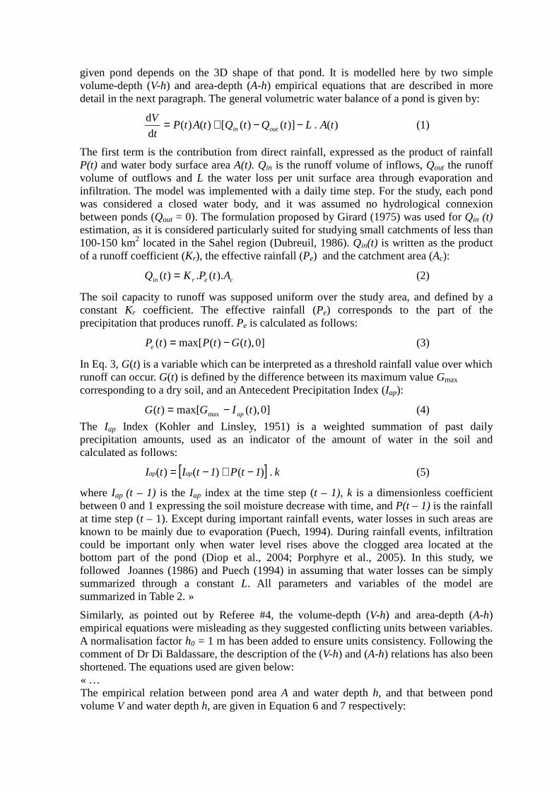
given pond depends on the 3D shape of that pond. It is modelled here by two simple volume-depth (V-h) and area-depth (A-h) empirical equations that are described in more detail in the next paragraph. The general volumetric water balance of a pond is given by:

)(.)]()([)()(d

dtALtQtQtAtP

t

Voutin −−+= (1)

The first term is the contribution from direct rainfall, expressed as the product of rainfall P(t) and water body surface area A(t). Qin is the runoff volume of inflows, Qout the runoff volume of outflows and L the water loss per unit surface area through evaporation and infiltration. The model was implemented with a daily time step. For the study, each pond was considered a closed water body, and it was assumed no hydrological connexion between ponds (Qout = 0). The formulation proposed by Girard (1975) was used for Qin (t) estimation, as it is considered particularly suited for studying small catchments of less than 100-150 km2 located in the Sahel region (Dubreuil, 1986). Qin(t) is written as the product of a runoff coefficient (Kr), the effective rainfall (Pe) and the catchment area (Ac):

cerin AtPKtQ ).(.)( = (2)

The soil capacity to runoff was supposed uniform over the study area, and defined by a constant Kr coefficient. The effective rainfall (Pe) corresponds to the part of the precipitation that produces runoff. Pe is calculated as follows:

]0),()(max[)( tGtPtPe −= (3)

In Eq. 3, G(t) is a variable which can be interpreted as a threshold rainfall value over which runoff can occur. G(t) is defined by the difference between its maximum value Gmax corresponding to a dry soil, and an Antecedent Precipitation Index (Iap):

]0),(max[)( max tIGtG ap−= (4)

The Iap Index (Kohler and Linsley, 1951) is a weighted summation of past daily precipitation amounts, used as an indicator of the amount of water in the soil and calculated as follows:

[ ] k1tP1tItI apap .)()()( −+−= (5)

where Iap (t – 1) is the Iap index at the time step (t – 1), k is a dimensionless coefficient between 0 and 1 expressing the soil moisture decrease with time, and P(t – 1) is the rainfall at time step (t – 1). Except during important rainfall events, water losses in such areas are known to be mainly due to evaporation (Puech, 1994). During rainfall events, infiltration could be important only when water level rises above the clogged area located at the bottom part of the pond (Diop et al., 2004; Porphyre et al., 2005). In this study, we followed Joannes (1986) and Puech (1994) in assuming that water losses can be simply summarized through a constant L. All parameters and variables of the model are summarized in Table 2. »

Similarly, as pointed out by Referee #4, the volume-depth (V-h) and area-depth (A-h) empirical equations were misleading as they suggested conflicting units between variables. A normalisation factor h0 = 1 m has been added to ensure units consistency. Following the comment of Dr Di Baldassare, the description of the (V-h) and (A-h) relations has also been shortened. The equations used are given below: « … The empirical relation between pond area A and water depth h, and that between pond volume V and water depth h, are given in Equation 6 and 7 respectively:

α

=

00

)()(

h

thStA (6)

1

00

)()(

+

=

α

h

thVtV with

100

0 +=

αhS

V (7)

where A(t) is the pond area at time t, h(t) is the pond water height at time t, S0 is the water area for h0 = 1 m water height in the pond (Table 2), α is a shape parameter representative of the slope profile (Table 2), V(t) is the volume of the pond at time t, V0 is the volume for h0 = 1 m water height in the pond. …»

3) Calibration and validation. In the former version, the model was calibrated using Barkedji pond that belongs to the main stream of Ferlo river (set 1) and then applied to all ponds, including those located outside the main stream (set 2). This was not considered appropriate as ponds inside and outside the main stream may have different hydrological behaviours. As suggested by Referee #1, two calibrations were made: one for the ponds inside the main stream (set 1) using water height data acquired on Barkedji pond in 2001 and another for the ponds outside the main stream (set 2) using water height measured on Furdu pond in 2002. The calibrations used daily rainfall recorded in 2001 and 2002 at a meteorological station located in Barkedji village. In the new version of the paper, two sets of parameters have thus been estimated and applied to their respective set of ponds. It must be pointed out that water height data used for calibration were not used for validation.

The calibration method itself was also not explained clearly enough in the previous version. In fact, no minimization methods were used here. Instead, we performed a systematic exploration of the input parameter space. Each parameter was allowed to vary with a fixed specified step within a range of values based on published literature. Each of the 6300 possible combinations were tested and ranked according to a calibration criterion. For the latter, we used the coefficient of efficiency (Nash and Sutcliffe, 1970) which is expressed as follows:

( )( )2

1

21

)()(

)()(1

iXiX

iXiXC

obsobsni

calobsni

eff

−

−−=∑∑

=

= with n = number of observed data

where Xobs is the observed data; Xcal is calculated with the model and obsX is the average

of the observed data. Nash–Sutcliffe efficiencies can range from −∞ to 1. The closer the coefficient of efficiency is to 1, the more accurate the model is.

Referees #1 and #4 then questioned the pertinence of using one Quickbird image to validate pond area simulation. Moreover, it was not clear for Dr Di Baldassare and Referee #1 which data sets were used respectively for model calibration and validation. In the revised version of the paper, we state that more clearly. We also explain that the validation procedure aimed to show that the model behaves ‘satisfactorily’ both temporally, on a limited number of ponds, and spatially, on all the ponds of the study area, while taking into account data availability in such data poor areas. By ‘satisfactorily’, we refer to the model’s ability to capture the trends in water level variations, and its applicability to a large number of ponds in the study area, given the intended use of the model as indicated

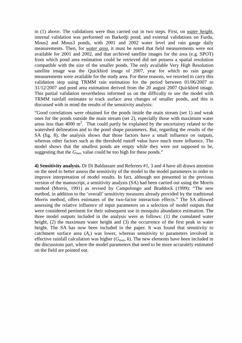
in (1) above. The validations were thus carried out in two steps. First, on water height, internal validation was performed on Barkedji pond, and external validations on Furdu, Mous2 and Mous3 ponds, with 2001 and 2002 water level and rain gauge daily measurements. Then, for water area, it must be noted that field measurements were not available for 2001 and 2002, and that archived satellite images for the area (e.g. SPOT) from which pond area estimation could be retrieved did not possess a spatial resolution compatible with the size of the smaller ponds. The only available Very High Resolution satellite image was the Quickbird image of 2007, year for which no rain gauge measurements were available for the study area. For these reasons, we resorted to carry this validation step using TRMM rain estimation for the period between 01/06/2007 to 31/12/2007 and pond area estimation derived from the 20 august 2007 Quickbird image. This partial validation nevertheless informed us on the difficulty to use the model with TRMM rainfall estimates to track surface area changes of smaller ponds, and this is discussed with in mind the results of the sensitivity analysis:

“Good correlations were obtained for the ponds inside the main stream (set 1) and weak ones for the ponds outside the main stream (set 2), especially those with maximum water areas less than 4000 m2. That could partly be explained by the uncertainty related to the watershed delineation and to the pond shape parameters. But, regarding the results of the SA (fig. 8), the analysis shows that those factors have a small influence on outputs, whereas other factors such as the threshold runoff value have much more influence. The model shows that the smallest ponds are empty while they were not supposed to be, suggesting that the Gmax value could be too high for these ponds.”

4) Sensitivity analysis. Dr Di Baldassare and Referees #1, 3 and 4 have all drawn attention on the need to better assess the sensitivity of the model to the model parameters in order to improve interpretation of model results. In fact, although not presented in the previous version of the manuscript, a sensitivity analysis (SA) had been carried out using the Morris method (Morris, 1991) as revised by Campolongo and Braddock (1999): “The new method, in addition to the ‘overall’ sensitivity measures already provided by the traditional Morris method, offers estimates of the two-factor interaction effects.” The SA allowed assessing the relative influence of input parameters on a selection of model outputs that were considered pertinent for their subsequent use in mosquito abundance estimation. The three model outputs included in the analysis were as follows: (1) the cumulated water height, (2) the maximum water height and (3) the occurrence of the first peak in water height. The SA has now been included in the paper. It was found that sensitivity to catchment surface area (Ac) was lower, whereas sensitivity to parameters involved in effective rainfall calculation was higher (Gmax, k). The new elements have been included in the discussions part, where the model parameters that need to be more accurately estimated on the field are pointed out.

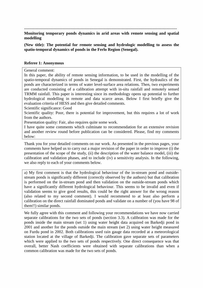
---------------------------------------------------------------------------------------------------------------- Monitoring temporary ponds dynamics in arid areas with remote sensing and spatial modelling

(New title): The potential for remote sensing and hydrologic modelling to assess the spatio-temporal dynamics of ponds in the Ferlo Region (Senegal).

Referee 1: Anonymous

General comment: In this paper, the ability of remote sensing information, to be used in the modelling of the spatio-temporal dynamics of ponds in Senegal is demonstrated. First, the hydraulics of the ponds are characterized in terms of water level-surface area relations. Then, two experiments are conducted consisting of a calibration attempt with in-situ rainfall and remotely sensed TRMM rainfall. This paper is interesting since its methodology opens up potential to further hydrological modelling in remote and data scarce areas. Below I first briefly give the evaluation criteria of HESS and then give detailed comments. Scientific significance: Good Scientific quality: Poor, there is potential for improvement, but this requires a lot of work from the authors. Presentation quality: Fair, also requires quite some work. I have quite some comments which culminate to recommendation for an extensive revision and another review round before publication can be considered. Please, find my comments below:

Thank you for your detailed comments on our work. As presented in the previous pages, your comments have helped us to carry out a major revision of the paper in order to improve (i) the presentation of the scope of the study, (ii) the description of the water balance model, (iii) the calibration and validation phases, and to include (iv) a sensitivity analysis. In the following, we also reply to each of your comments below. a) My first comment is that the hydrological behaviour of the in-stream pond and outside-stream ponds is significantly different (correctly observed by the authors) but that calibration is performed on the in-stream pond and then validation on the outside-stream ponds which have a significantly different hydrological behaviour. This seems to be invalid and even if validation seems to give good results, this could be the right answer for the wrong reason (also related to my second comment). I would recommend to at least also perform a calibration on the direct rainfall dominated ponds and validate on a number of (you have 98 of them!!) similar ponds.

We fully agree with this comment and following your recommendations we have now carried separate calibrations for the two sets of ponds (section 3.3). A calibration was made for the ponds inside the main stream (set 1) using water height data acquired on Barkedji pond in 2001 and another for the ponds outside the main stream (set 2) using water height measured on Furdu pond in 2002. Both calibrations used rain gauge data recorded at a meteorological station located at the village of Barkedji. The calibration gave separate sets of parameters which were applied to the two sets of ponds respectively. One direct consequence was that overall, better Nash coefficients were obtained with separate calibrations than when a common calibration was made for the two sets of ponds.

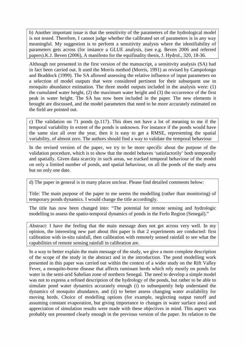
b) Another important issue is that the sensitivity of the parameters of the hydrological model is not tested. Therefore, I cannot judge whether the calibrated set of parameters is in any way meaningful. My suggestion is to perform a sensitivity analysis where the identifiability of parameters gets across (for instance a GLUE analysis, (see e.g. Beven 2006 and referred papers).K.J. Beven (2006), A manifesto for the equifinality thesis, J. Hydrol., 320, 18-36.

Although not presented in the first version of the manuscript, a sensitivity analysis (SA) had in fact been carried out. It used the Morris method (Morris, 1991) as revised by Campolongo and Braddock (1999). The SA allowed assessing the relative influence of input parameters on a selection of model outputs that were considered pertinent for their subsequent use in mosquito abundance estimation. The three model outputs included in the analysis were: (1) the cumulated water height, (2) the maximum water height and (3) the occurrence of the first peak in water height. The SA has now been included in the paper. The new elements it brought are discussed, and the model parameters that need to be more accurately estimated on the field are pointed out. c) The validation on 71 ponds (p.117). This does not have a lot of meaning to me if the temporal variability in extent of the ponds is unknown. For instance if the ponds would have the same size all over the year, then it is easy to get a RMSE, representing the spatial variability, of almost zero. The authors should find a way to validate the temporal behaviour

In the revised version of the paper, we try to be more specific about the purpose of the validation procedure, which is to show that the model behaves ‘satisfactorily’ both temporally and spatially. Given data scarcity in such areas, we tracked temporal behaviour of the model on only a limited number of ponds, and spatial behaviour, on all the ponds of the study area but on only one date. d) The paper in general is in many places unclear. Please find detailed comments below: Title: The main purpose of the paper to me seems the modelling (rather than monitoring) of temporary ponds dynamics. I would change the title accordingly.

The title has now been changed into: “The potential for remote sensing and hydrologic modelling to assess the spatio-temporal dynamics of ponds in the Ferlo Region (Senegal).” Abstract: I have the feeling that the main message does not get across very well. In my opinion, the interesting new part about this paper is that 2 experiments are conducted: first calibration with in-situ rainfall, then calibration with remotely sensed rainfall to see what the capabilities of remote sensing rainfall in calibration are.

In a way to better explain the main message of the study, we give a more complete description of the scope of the study in the abstract and in the introduction. The pond modelling work presented in this paper was carried out within the context of a wider study on the Rift Valley Fever, a mosquito-borne disease that affects ruminant herds which rely mostly on ponds for water in the semi-arid Sahelian zone of northern Senegal. The need to develop a simple model was not to express a refined description of the hydrology of the ponds, but rather to be able to simulate pond water dynamics accurately enough (i) to subsequently help understand the dynamics of mosquito abundance, and (ii) to better assess changing water availability for moving herds. Choice of modelling options (for example, neglecting output runoff and assuming constant evaporation, but giving importance to changes in water surface area) and appreciation of simulation results were made with these objectives in mind. This aspect was probably not presented clearly enough in the previous version of the paper. Its relation to the

other important aspect of the study, on investigating the potentiality of remote sensing data to support hydrological modelling in data poor areas, is also more clearly stated. Furthermore, could you clarify whether the validation with Quickbird imagery was done for both experiments or not? Does the ‘pond map’ contain water surfaces for all ponds at one moment in time?

The validation with Quickbird imagery was done for simulations using TRMM rainfall. For pond surface validation, it must be noted that field measurements were not available for 2001 and 2002, and that archived satellite images for the area (e.g. SPOT) from which pond area estimation could be retrieved did not possess a spatial resolution compatible with the size of the smaller ponds. The only available Very High Resolution satellite image was the Quickbird image of 2007, year for which no rain gauge measurements were available for the study area. For these reasons, we resorted to carry this validation step using TRMM rain estimation for the period between 01/06/2007 to 31/12/2007 and pond area estimation derived from the 20 august 2007 Quickbird image. This partial validation nevertheless informed us on the difficulty to use the model with TRMM rainfall estimates to track surface area changes of smaller ponds, and this is discussed with in mind the results of the sensitivity analysis. p.105, L. 7 “inventory” ! “characterize”

“inventory” was replaced by “characterize” p. 105, L. 10. I recommend a reference to the following interesting paper. That uses remotely sensed water surfaces to calibrate a hydrological model. J. R. Liebe, N. van de Giesen, M. Andreini, M. T. Walter, and T. S. Steenhuis (2009), Determining watershed response in data poor environments with remotely sensed small reservoirs as runoff gauges, Water Resour. Res., 45, W07410, doi:10.1029/2008WR007369.

Thank you very much for bringing to our attention the works of Dr Liebe et al. They have been cited at different places in the introduction to give a more complete overview of past and present efforts in hydrological modelling that uses remote sensing in data poor areas. p.105, L.21 “was” ! “is” “was” was replaced by “is” p.106, L.6, something is missing; and p.106, L.7: “uses”! “use”:

The sentence contained in lines 6 and 7 has been reworded: “In order to access additional temporal information on pond dynamics, hydrologic models have been developed at the pond scale (Desconnets, 1994; Desconnets et al., 1997; Martin-Rosales and Leduc, 2003). Applications at a regional scale to monitor states of daily water bodies have also been tested with success.” p.106, L.9: these relations are purely mathematical.

“Volume-Depth-Area hydrologic mathematical relations” was replaced by “Volume-Depth-Area mathematical relations”

p.106, L.14: “Difficulty to generalize”! “difficulty generalizing” p.106, L.25: relatively simple: relative to what?

The introduction has changed such that “Difficulty to generalize” and “relatively simple” are

absent. p.107.L.1. Why were extensive flood events omitted?

Extensive flood events are very unusual in that area. They are also quite difficult to model, and incompatible with the simplicity of model. p.107.L.13 “Ferlo River”

The word “River” has been added after “Ferlo”. p.107.L.26: Add the word “event”

“event” was added in the sentence, after “precipitation”. p.108 L17: Why was the 2001 data of Barkedji not used?

In the section 2 “Data description”, we explain why the 2001 field data for Barkedji pond was not used. “For Barkedji, the water level readings for the first season (2001) were unexploitable due to a technical problem (displacement of the meter) that was not detected and corrected early enough. Therefore, only water height data collected during the 2002 rainy season were used.” p.109. L.1. A lot of details are missing. The pond maps were not extracted is my guess. They were post-processed from the raw imagery. Please explain how this was done. I’m not sure how you can extract a pond catchment area from a visual image. This is usually done with a DEM. How was the maximum surface area derived??

The pond maps were derived from Quickbird satellite images by thresholding a water index computed from two of their wavebands (green and near infrared). In this study, we used the Normalized Difference Water index (NDWI; Mc Feeters, 1996) which is known to be suited for the extraction of water bodies (Soti et al., 2009). The index is calculated as the difference between the green and the near infrared bands, and normalised by their sum.

One of the main input parameters of the model is the pond catchment area Ac. This parameter was estimated differently for ponds of sets 1 and 2. For ponds inside the main stream (set 1) which are larger, the catchment areas (with slopes up to 8%) could be reconstructed from ASTER DEM data. However for ponds outside the main stream (set 2), where ponds are generally much smaller, slopes were too plat to be detected in available DEM. Therefore, for this set of ponds, we empirically estimated the catchment area of a given pond as n times the maximum water surface area of that pond; n being an integer, obtained during the calibration phase as a constant value for all ponds of set 2. The maximum surface area of ponds were read directly from the pond map corresponding to the August 4th, 2005 Quickbird image. That image was acquired at the peak of a higher than normal rainfall season, when ponds were expected to be at their maximum.

p.110. L.1 Start by giving the water balance equation of the pond, for instance:

))()()()(d

dtLAAtPKtAtP

t

Scer −+= (1)

It seems to me that a flux is missing. Outflow from the pond by the surface. In the riverine ponds, this may be very important.

All of the suggestions for improving the presentation of the water balance equation have been taken into account. The new version is given in extenso above. Please refer to Major Changes (2: Hydrologic model description).

)(.)]()([)()(d

dtALtQtQtAtP

t

Voutin −−+= (a)

The outflow term Qout is now present in the water balance equation. However, ponds were assumed to be unconnected, such that the outflow terms were neglected. This approximation is justified by the simplicity of the model and its intended use, but also by the difficulty of modelling pond interconnection, both conceptually, and because of lack of data. The symbol ∆V for runoff is confusing as it is usually reserved for a change in Volume. ∆ suggests a change in something.The symbol Q is more common for runoff. Eq.1 is also not the equation for ‘the runoff value’ but an equation for the inflow. Please change accordingly. Also ER cannot be a symbol as it mathematically means ‘E*R’. You could use Pe (e as subscript) for effective rainfall.

cerin AtPKtQ ).(.)( = (b)

Q is now used for inflow. ER has been replaced by Pe.

Eq.1. I recommend writing the differential equation instead of its solution (Euler explicit). So please write (for instance)

cer AtPKtAtPt

S)()()(

d

d += (2)

The water balance equation is now written in the form of a differential equation (see equation (a) and (b) above). eq. 3 Write with a max operator:

]0),()0(max[)( tIMtM ap−= (3)

Is this really correct, should it not be dM/dt = Iap(t) ? Why not simply use a soil moisture state to cater for antecedent conditions?

]0),(max[)( max tIGtG ap−= (c)

As suggested, we now use the max operator notation. However, in the previous version, the meaning of M was not clearly given (“… time dependent soil moisture variable”) and was inevitably mistaken for moisture. In the new version, we use variable G instead of M, and define it unambiguously: “In Eq. 3, G(t) is a variable which can be interpreted as a threshold rainfall value over which runoff can occur. G(t) is defined by the difference between its maximum value Gmax corresponding to a dry soil, and an Antecedent Precipitation Index (Iap).” p. 111, L.6: “API has no regional meaning”. But it does!! It is a measure for memory of the catchment which can vary considerably as a function of slope, soil moisture capacity, etc

By “API has no regional meaning”, we meant that, as Anctil et al. (2004) pointed out, API (now, Iap) is spatially variable and cannot be transposed between sites, even within the same region. We have now removed the expression “regional meaning” and have been more direct in our explanation: “Because of the high spatial variation of the precipitation, the Iap(t) index is also spatially variable within the Sahel and, as such, cannot be compared between sites”. p. 111, L.9: “lower values for Sahelian regions” Explain why. My guess is there is a higher evaporation potential which causes dryer conditions and thus in general lower APIs.

Yes, that is right. In the text, we added an explanation on why k is lower in the Sahelian region as follows: “The k parameter generally ranges between 0.80 and 0.98 (Heggen, 2001) but takes lower values for the Sahelian region (Girard, 1975) because of a high evapotranspiration potential (around 250 mm per month)”.

p.112 eq. 6: It is not clear with respect to what reference level ht should be given.

The reference level for water height in a pond is the lowest point of that pond. This was not given in the previous version. It has now been added. p.113. L-2-3: Omit “for one pond: : :.between A and h”

Sentence was omitted. p. 113 L. 17: Omit which software was used.

Software name was omitted from the text. p. 114, L. 5: eq. 9, is incorrect. should be something like 1 - σobs/cal / σ obs

Yes, the Nash-Sutcliffe equation was corrected as follows:

( )( )2

1

21

)()(

)()(1

iXiX

iXiXC

obsobsni

calobsni

eff

−

−−=∑∑

=

= (d)

where n = number of observed data, Xobs is the observed data; Xcal is calculated with the model

and obsX is the average of the observed data.

p.114, L.5 : What data was used for Vobs? There were no observations available for this variable so how can it be used for calibration? Why not use h? In the figures, A is given. I’m confused:

Our choice of notations and of the variable to be plotted in figure 6 was not appropriate. Water height data were in fact used for validation. The use of V in the definition of the Nash-Sutcliffe coefficient was confusing and has therefore been replaced by X (see also Major changes (3: Calibration and validation)). In Figure 6 of the previous version, although not measured, ‘observed’ pond surface area (A) could be plotted because they were calculated from measured heights using the A-h relationship. But we agree that this may also be confusing. Therefore in Figure 6 we now compare water height measurements with water height simulations using rain gauge and TRMM rainfall data as input to the model.

p.114, L.18: “realistic range based on scientific knowledge”. What knowledge? This is not at all supported, at least a reference should be given to this knowledge or the evidence should be given here.

We have replaced “on scientific knowledge” by “on published literature as given in table 2”. All references are listed in the “reference column” in table 2. p. 115 eq.10: Why was this radius calculated?? L. 3-6 are not clear to me. What is the ‘negative buffer radius’.

The description of the link with the GIS and the calculation of a radius were to explain how to represent the comparison between a simulated pond surface area and the pond surface area observed in the satellite image. The observed pond surface areas are represented by polygons in the GIS. The simulated pond surface areas obtained were generally less than the observed ones. To represent the simulated pond surface area, we applied a buffer to the observed pond polygons to trim them to the required (simulated) surface area. Pond ‘radius’ calculation was necessary for obtaining the thickness of the buffer to be applied for each pond. We agree that the explanations were not clear enough, nor were they placed at the appropriate place. Therefore, they have been removed in the new version. A short explanation was however added in the Figure 7b legend. p.115 l. 11. Nash and RMSE describe in fact the same variability. The only difference is that Nash scales the errors over the variance of the observations. Please omit one of the two. If you refer here to eq.9, then please describe eq. 9 in general terms (not for volume specifically).

The Nash-Sutcliffe coefficient is normally used when comparing simulations of a hydrological model, against time series measurements. This coefficient was therefore used as the criterion for evaluating pond water height simulations for the 2001 and 2002 rainy seasons. However, for pond area simulation, evaluation was done for only one date (20 August 2007: Quickbird image acquisition date) but for 98 ponds. For such an evaluation the RMSE is more commonly prescribed. In equation 9 which defines the Nash-Sutcliffe coefficient, the notation has been changed (V replaced by X) to express the definition in general terms. Please refer to Major changes (3: calibration and validation) and equation (d) above. p.116. I’m wondering: if the GPS survey is so detailed, why then do you need the power laws?

Detailed DEM / bathymetry were available only for two ponds: Niaka and Furdu. They were obtained during ground surveys using a Theodolite total station. Niaka is a larger pond belonging to set 1, and Furdu, a smaller one, belonging to set 2. The power laws have been used to summarize the shape of any pond into two parameters S0 and α. Then, the detailed DEM of Niaka and Furdu were used to estimate the two parameters for each set of ponds, assuming that Niaka is representative of set 1 and Furdu of set 2. In this way, the model could be applied to all the ponds for which a detailed DEM / bathymetry were not available. p.116. L.13: How was calibration performed? Manually? As mentioned in my comments, I cannot judge the identifiability of any parameter value here. This needs additional work.

The calibration method itself was not given in the previous version. As the model requires only limited computing power, it was not found necessary to use any dedicated error function minimisation methods (Simplex, Powell,...). Instead, we simply scanned the whole parameter

space with a fixed step for each parameter, retaining the set of parameter values that maximized a chosen ‘quality’ criterion. For that, we also used the Nash-Sutcliffe coefficient. The table below shows the model parameters on which the calibration was carried out and the corresponding range of values explored. In the new version, Section 3.4 (Model calibration) has been changed to include the description of the calibration method and the table containing the calibration experimental plan. Table I: Calibration experimental plan

Parameter Min Max Step Nb Kr 0.17 0.23 0.01 7 Gmax (mm/day) 13 15 1 3 k 0.4 0.6 0.1 3 L (mm/day) 12 16 1 5 n 1 20 1 20

Total run: 6300 Table 1. mention the months as well as years of acquisition. replace ‘extracted’ by ‘derived’, the water level data is missing!!

Complete dates of data acquisition periods are now given in Table 1. “extracted” was replaced by “derived”. Water height data was present in the former table. However, the horizontal line that separates TRMM rainfall data and water height data was missing. This may explain the confusion, and has been corrected. Table 2. Units are not clear everywhere. Rainfall is a flux and thus effective rainfall cannot be a state variable and should have a unit L/T (e.g. mm/hr). The range of values (0<P<0.045) can therefore not be interpreted.

In Table 2 of the previous version, the values were given having in mind a daily time step. In the new version below, non state variables have been removed and appropriate units have been included.

Table II: Parameters and variables of the hydrologic pond model

Abbreviation Parameters and variables Value/Range of values /equation Unit Reference

Input variables

P Rainfall 0 < P < 45 mm/day Field survey

State variables

V Pond volume Eq.1 m3

A Pond surface area Eq.6 m2

h Pond water height Eq.7 m

Parameters

Ac Catchment area 0 - 150 km2 (Dubreuil, 1986) Kr Runoff coefficient 0.15 - 0.40 - (Girard, 1975) α Water body shape factor 1 - 3 - (FAO, 1996; Puech

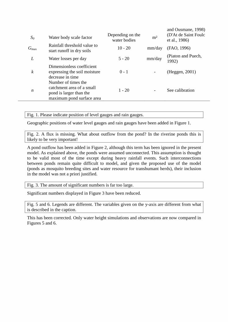
and Ousmane, 1998)

S0 Water body scale factor Depending on the

water bodies m²

(D'At de Saint Foulc et al., 1986)

Gmax Rainfall threshold value to start runoff in dry soils

10 - 20 mm/day (FAO, 1996)

L Water losses per day 5 - 20 mm/day (Piaton and Puech, 1992)

k Dimensionless coefficient expressing the soil moisture decrease in time

0 - 1 - (Heggen, 2001)

n

Number of times the catchment area of a small pond is larger than the maximum pond surface area

1 - 20 - See calibration

Fig. 1. Please indicate position of level gauges and rain gauges.

Geographic positions of water level gauges and rain gauges have been added in Figure 1. Fig. 2. A flux is missing. What about outflow from the pond? In the riverine ponds this is likely to be very important!

A pond outflow has been added in Figure 2, although this term has been ignored in the present model. As explained above, the ponds were assumed unconnected. This assumption is thought to be valid most of the time except during heavy rainfall events. Such interconnections between ponds remain quite difficult to model, and given the proposed use of the model (ponds as mosquito breeding sites and water resource for transhumant herds), their inclusion in the model was not a priori justified. Fig. 3. The amount of significant numbers is far too large.

Significant numbers displayed in Figure 3 have been reduced. Fig. 5 and 6. Legends are different. The variables given on the y-axis are different from what is described in the caption.

This has been corrected. Only water height simulations and observations are now compared in Figures 5 and 6.

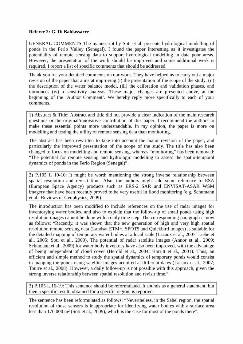
Referee 2: G. Di Baldassarre GENERAL COMMENTS The manuscript by Soti et al. presents hydrological modelling of ponds in the Ferlo Valley (Senegal). I found the paper interesting as it investigates the potentiality of remote sensing data to support hydrological modelling in data poor areas. However, the presentation of the work should be improved and some additional work is required. I report a list of specific comments that should be addressed.

Thank you for your detailed comments on our work. They have helped us to carry out a major revision of the paper that aims at improving (i) the presentation of the scope of the study, (ii) the description of the water balance model, (iii) the calibration and validation phases, and introduces (iv) a sensitivity analysis. These major changes are presented above, at the beginning of the ‘Author Comment’. We hereby reply more specifically to each of your comments. 1) Abstract & Title: Abstract and title did not provide a clear indication of the main research questions or the original/innovative contribution of this paper. I recommend the authors to make these essential points more understandable. In my opinion, the paper is more on modelling and testing the utility of remote sensing data than monitoring.

The abstract has been rewritten to take into account the major revision of the paper, and particularly the improved presentation of the scope of the study. The title has also been changed to focus on modelling and remote sensing, whereas “monitoring” has been removed: “The potential for remote sensing and hydrologic modelling to assess the spatio-temporal dynamics of ponds in the Ferlo Region (Senegal)”. 2) P.105 L 10-16: It might be worth mentioning the strong inverse relationship between spatial resolution and revisit time. Also, the authors might add some reference to ESA (European Space Agency) products such as ERS-2 SAR and ENVISAT-ASAR WSM imagery that have been recently proved to be very useful in flood monitoring (e.g. Schumann et al., Reviews of Geophysics, 2009).

The introduction has been modified to include references on the use of radar images for inventorying water bodies, and also to explain that the follow-up of small ponds using high resolution images cannot be done with a daily time-step. The corresponding paragraph is now as follows: “Recently, it was shown that the new generation of high and very high spatial resolution remote sensing data (Landsat ETM+, SPOT5 and Quickbird images) is suitable for the detailed mapping of temporary water bodies at a local scale (Lacaux et al., 2007; Liebe et al., 2005; Soti et al., 2009). The potential of radar satellite images (Annor et al., 2009; Schumann et al., 2009) for water body inventory have also been improved, with the advantage of being independent of cloud cover (Herold et al., 2004; Horritt et al., 2001). Thus, an efficient and simple method to study the spatial dynamics of temporary ponds would consist in mapping the ponds using satellite images acquired at different dates (Lacaux et al., 2007; Tourre et al., 2008). However, a daily follow-up is not possible with this approach, given the strong inverse relationship between spatial resolution and revisit time.” 3) P.105 L.16-19: This sentence should be reformulated. It sounds as a general statement, but then a specific result, obtained for a specific region, is reported.

The sentence has been reformulated as follows: “Nevertheless, in the Sahel region, the spatial resolution of those sensors is inappropriate for identifying water bodies with a surface area less than 170 000 m² (Soti et al., 2009), which is the case for most of the ponds there”.

4) P.109 L 5-7: It is not clear why this image is used for evaluating the maximum surface area. The paper should state here what is reported in p.114 line 9.

For ponds outside the main stream (set 2), where slopes are too plat to be detected in available DEM, catchment areas were empirically estimated as n times the maximum water surface area of that pond; n being an integer and obtained through calibration. In the previous version, n, the catchment/pond surface area ratio, was set to 9 (or the radius ratio to 3). Following comments by several Referees we have removed this arbitrary parameter setting, and estimated it during the calibration phase (a value of 10 was then obtained). The maximum surface area of ponds were obtained with the pond map corresponding to the August 4th, 2005 Quickbird image. That image was acquired at the peak of a higher than normal rainfall season, when ponds were expected to be at their maximum. In the part describing pond maps, we have now added for what purpose the maximum pond surface areas were derived from the 2005 Quickbird satellite image. 5) P.109 L. 14: The authors should explain what they exactly mean by "usual events".

In the former version, we wanted to express that the rare exceptional rainfall events which cause flooding (and ponds to temporarily merge during the event) were not taken into account in the model. This sentence has been removed in the new version. 6) P.110 L. 9: The balance equation is not entirely clear to me. This is partly due to the notation (see other comments below).

The presentation of the water balance model has significantly changed. In particular, it is now given as a differential equation, without separating it into a ‘pond filling’ and a ‘pond emptying’ model. Wherever necessary, more appropriate notations have also been used. Please refer to Major changes (2: Hydrologic model description) above. 7) P.111-113: This part should be revised. Surely, it is not clear why the description of trivial volume-depth relationships is longer than the description of the hydrological model.

The hydrological model presentation has been rewritten to be more complete, and the description of the volume-area depth relationships has been restrained to how they have been employed in this study. 8) P.114 L.11-20: I could not understand how the model was calibrated. Did the authors use the volume, the area or the water depths? Is Vobs the observed pond volume? Are there observations of pond volume? Why does Figure 5 plot the area? And why figure’s caption states water heights?

The calibration method was not described in the previous version. As the model requires only limited computing power, it was not found necessary to use any dedicated error function minimisation methods (Simplex, Powell, ...). Instead, we simply scanned the whole parameter space with a fixed step for each parameter, retaining the set of parameter values that maximized a chosen ‘quality’ criterion. For that, we also used the Nash-Sutcliffe coefficient. The Table I above gives the model parameters on which the calibration was carried out and the corresponding range of values explored. In the new version, Section 3.4 (Model calibration) has been changed to include the description of the calibration method and the table containing the calibration experimental plan (Table I). The calibration was carried out using only water height measurements, and no pond volume observations were available. The Vobs notation used in the definition of the Nash-Sutcliffe coefficient was confusing. In the new

version, we use X instead of V to keep the definition of the coefficient general, but applied it using h during the calibration phase. In Figures 5 and 6, only water height measurements and simulations are now compared. 9) P.114 L. 6-7: Is this arbitrary (and rather questionable) assumption plausible? And is it actually necessary?

In available DEM, it was not possible to extract catchment areas of the ponds outside the main stream (set 2). These ponds are smaller than those in the main stream, and the slopes in their catchment areas are almost plat. In the model, the catchment area of such a pond was empirically estimated as n times the maximum water surface area of that pond; n being an integer. In the previous version, n, the catchment/pond surface area ratio, was set to 9 (or the radius ratio to 3), arbitrarily, without anymore justification than being plausible according to ‘expert knowledge’. However, following comments by several Referees we have now removed this arbitrary parameter setting, and estimated it as one more input parameter during the calibration phase (a value of n = 10 was then obtained). The assumption of a simple relation between catchment area and maximum pond area for small ponds was necessary as we did not have any other means to estimate catchment area. In the sensitivity analysis, it was found, however, that sensitivity to catchment surface area (Ac) was lower, suggesting that this simplification may not be too penalizing. 10) P.113-116: Perhaps, I have missed something, I could not understand exactly how the parameters were estimated, calibrated, evaluated, validated and then used for different ponds.

We agree that the calibration and validation phases were not clearly described in the previous version. Also, following a comment from Referee 1, it was suggested that separate calibration should be carried out for ponds of set 1 and set 2. These changes to the calibration and validation phases are described at the beginning of the ‘Author Comment’ (Major changes (3: Calibration and validation) above. The main lines are summarized hereby:

• Two calibrations were made following the method described in the response to comment #8 above, one using water height data acquired on Barkedji pond in 2001 for ponds of set 1, and another using water height measured on Furdu pond in 2002 for ponds of set 2. Both calibrations used gauge rainfall measurements.

• Table III below shows the parameter values resulting from the calibration:

Parameters Barkedji (set 1) Furdu (set 2) Kr 0.21 0.19

Gmax (mm/day) 15 15 k 0.4 0.5

L (mm/day) 15 12 n - 10

Nash coef. 0.82 0.87

• These parameters were used to run the model for all the ponds of each set. The catchment area of each pond was obtained differently depending on the set of pond it belongs to. For ponds of set 1, catchment areas were obtained from ASTER DEM, whereas for ponds of set 2, catchment areas were estimated as n times the maximum pond surface, as observed on the August 4th, 2005 Quickbird image. That image was acquired at the peak of a higher than normal rainfall season, when ponds were expected to be at their maximum.

• The validation was carried out with data not used for calibration. Given data scarcity

in such areas, the temporal behaviour of the model was validated using measured water heights on only a limited number of ponds (Barkedji, Furdu, Mous2 and Mous3 ponds), and spatial behaviour, on all the ponds of the study area but on only one date, using pond area as observed in the 20th august 2007 Quickbird image. For temporal behaviour, rain gauge measurements of 2001 and 2002 were used, but for 2007, no rain gauge measurements were available. We therefore resorted to carry this pond area part of the validation using TRMM rain estimation for the period between 01/06/2007 to 31/12/2007.

11) Eq.10: I think that the formula is not needed

Equation 10 has been removed from the text which was anyhow changed to take into account other comments on model calibration.

12) P.117 L.16-18: The paper should state how the QuickBird image was processed to derive lake extent areas. Please note that different results can be obtained using different procedures (e.g. Di Baldassarre et al., Journal of Hydrology, 2009).

Pond extent areas were derived from Quickbird satellite images by thresholding a water index computed from two of their wavebands (green and near infrared). The water index used is the Normalized Difference Water index (NDWI; Mc Feeters, 1996) which is known to be suited for the extraction of water bodies (Soti et al., 2009). The index is calculated as the difference between the green and the near infrared bands, and normalised by their sum. This has been added in the “Materials and methods / Pond maps” section, and the suggested reference is cited in the introduction.

13) P.117 L.18-20: It is not clear to me what type of correlation measure was used by the authors. The scientific literature provides many performance measures to compare observed areas to simulated areas (e.g. Horritt et al., Hydrological Processes, 2007), none of them seem to be used here.

Unlike in the suggested reference, we compared simulated pond areas to those observed in a very high resolution satellite image, only for one date, but for 98 ponds. The most commonly used model performance measures were then used: RMSE and R². 14) Discussion & Conclusions: Given the way how good or poor outcomes are presented, they seem to be the result of fortunate or unfortunate coincidences. This is mainly due to the lack of a sensitivity analysis, as pointed out by the Anonymous Reviewer. Also, why the 2001 results are not showed? I do not understand the tendency to present only good results. In fact, I do not believe that nowadays the hydrological community reads HESS only to see how well a model developed 35 years ago fits observed data in a specific test site. I would recommend focussing more on the poor results. For instance, it might be interesting to know why the use of TRMM data for the 2001 event led to poor results.

The “Discussion and Conclusions” has significantly changed following the “Major changes” (1-4) described above. In particular, the scope of the study has been described more explicitly, a sensitivity analysis has been included, and the calibration was carried out separately for ponds of set 1 and set 2. These changes have led us to change the discussion of the results and the conclusions drawn from them.

Water level measurements were made during the rainy seasons of 2001 and 2002 in four

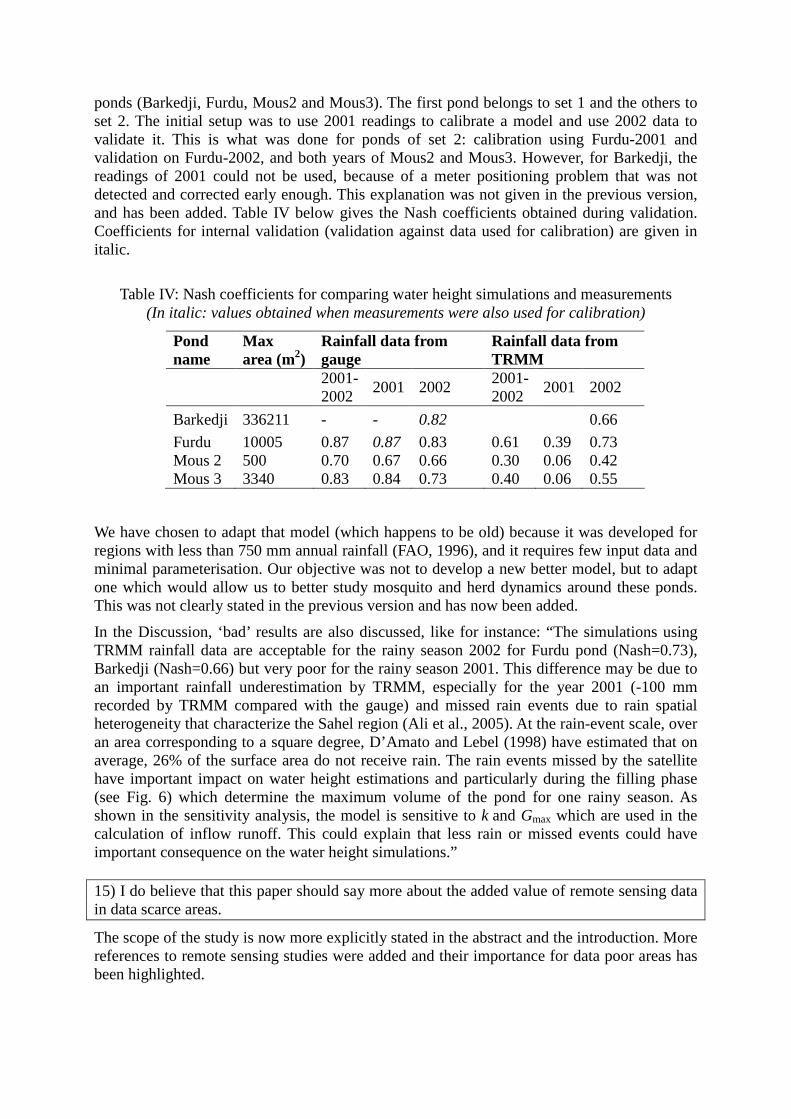
ponds (Barkedji, Furdu, Mous2 and Mous3). The first pond belongs to set 1 and the others to set 2. The initial setup was to use 2001 readings to calibrate a model and use 2002 data to validate it. This is what was done for ponds of set 2: calibration using Furdu-2001 and validation on Furdu-2002, and both years of Mous2 and Mous3. However, for Barkedji, the readings of 2001 could not be used, because of a meter positioning problem that was not detected and corrected early enough. This explanation was not given in the previous version, and has been added. Table IV below gives the Nash coefficients obtained during validation. Coefficients for internal validation (validation against data used for calibration) are given in italic.

Table IV: Nash coefficients for comparing water height simulations and measurements

(In italic: values obtained when measurements were also used for calibration)

Pond name

Max area (m2)

Rainfall data from gauge

Rainfall data from TRMM

2001-2002

2001 2002 2001-2002

2001 2002

Barkedji 336211 - - 0.82 0.66

Furdu 10005 0.87 0.87 0.83 0.61 0.39 0.73 Mous 2 500 0.70 0.67 0.66 0.30 0.06 0.42 Mous 3 3340 0.83 0.84 0.73 0.40 0.06 0.55

We have chosen to adapt that model (which happens to be old) because it was developed for regions with less than 750 mm annual rainfall (FAO, 1996), and it requires few input data and minimal parameterisation. Our objective was not to develop a new better model, but to adapt one which would allow us to better study mosquito and herd dynamics around these ponds. This was not clearly stated in the previous version and has now been added.

In the Discussion, ‘bad’ results are also discussed, like for instance: “The simulations using TRMM rainfall data are acceptable for the rainy season 2002 for Furdu pond (Nash=0.73), Barkedji (Nash=0.66) but very poor for the rainy season 2001. This difference may be due to an important rainfall underestimation by TRMM, especially for the year 2001 (-100 mm recorded by TRMM compared with the gauge) and missed rain events due to rain spatial heterogeneity that characterize the Sahel region (Ali et al., 2005). At the rain-event scale, over an area corresponding to a square degree, D’Amato and Lebel (1998) have estimated that on average, 26% of the surface area do not receive rain. The rain events missed by the satellite have important impact on water height estimations and particularly during the filling phase (see Fig. 6) which determine the maximum volume of the pond for one rainy season. As shown in the sensitivity analysis, the model is sensitive to k and Gmax which are used in the calculation of inflow runoff. This could explain that less rain or missed events could have important consequence on the water height simulations.” 15) I do believe that this paper should say more about the added value of remote sensing data in data scarce areas.

The scope of the study is now more explicitly stated in the abstract and the introduction. More references to remote sensing studies were added and their importance for data poor areas has been highlighted.

16) The English should be improved as well; I would recommend double checking the text before re-submission and ask a native speaker to proof read the manuscript.

The “Author Comment” has been checked and corrected for English. The same is being done for the manuscript. 17) In my opinion, the use of the personal form ("we" and "our") is redundant. Personally, I do not like the expressions as "in our study area" or the rather informal "as we can see".

Most of the personal forms have been removed from the text.

Referee 3: Anonymous 1) General comment : Content/subject/title The paper investigates the potential for an approach combining remote sensing of both rainfall and surface water and hydrological modelling to assess the spatio-temporal variability of ponds in the Ferlo region (Senegal). The structure of the manuscript consists of an introduction that sets the overall framework of the study in an area with obvious data scarcity, a section that describes the study area and available data sets (meteorological, hydrological, topographic, remote sensing images), a methodology section where a daily water balance model and a volume-area-depth model are described, results and discussion sections, as well as a general conclusion.

We would like to thank you for your careful review of our work. Your detailed comments have helped us carry out a major revision of the paper that includes (i) a more appropriate presentation of the scope of the study, (ii) a more rigorous description of the water balance model, (iii) reworked calibration and validation phases, and (iv) a sensitivity analysis. These major changes are presented at the beginning of the ‘Author Comment’. We also reply to your specific comments below. 2) The title of the paper appeared somewhat misleading, in the sense that ponds dynamics are said to be monitored a.o. via remote sensing and spatial modelling. I would suggest to clearly distinguish between monitoring and modelling. As I understand, the main issue in this paper is the data scarcity, which calls for the use of innovative approaches that will in the end allow for a better quantitative and qualitative management of water resources in the area under investigation. The title should thus highlight the potential for remote sensing and hydrologic modelling to assess the spatio-temporal dynamics of ponds in the Ferlo Region (Senegal).

We agree with your comment on the need to find a more appropriate title for the paper and following your suggestion we have changed the title to: “The potential for remote sensing and hydrologic modelling to assess the spatio-temporal dynamics of ponds in the Ferlo Region (Senegal)”. 3) Study area/data/methodology : While the interest of the study is quite obvious in the area under investigation, the description and discussion of the available data sets appears to be somewhat too superficial at this stage. The authors rely for example on rainfall measurements obtained both through ground based measurements and satellite borne remote sensing (TRMM). It would be very useful to further discuss the accuracy of those measurements, i.e. the scarcity of the rain gauges, the precision of the TRMM data, differences between the two measurement series, etc.

We give more justification for this study by describing the context within which the pond modelling work has been carried out. The issue is about the Rift Valley fever, a mosquito borne disease that affects herds in this area. The herds come to feed and drink near the ponds, just where the mosquitoes develop. The dynamics of mosquito abundance is not well explained by rainfall only. It is more linked to the development phases of two mosquito species (Aedes and Culex) that have different behaviours relative to pond dynamics. What is expected from the model is to give a good indication of water availability in the pond for herds, and more importantly, it has to simulate on a daily basis the changes in pond surface area to which mosquito abundance is related. For example, Aedes mosquitoes lay eggs in damp soil around the ponds and the eggs hatch only after a sequence of dry and wet conditions. In the new version, the scope of the study now includes this aspect, and it explains

some of the modelling choices we have made. The model was run using gauge rainfall measurements as input, but knowing the difficulty to have gauge measurements wherever necessary, we tested rainfall estimated from satellite as input to the model. Although TRMM tend to underestimate rainfall, the timing is usually correct. For this reason, it is expected that model simulation for mosquito abundance would not suffer a lot from this underestimation problem. This discussion has been added to the text. Additional technical information is also provided concerning TRMM data and gauge measurements. One interesting information in this context is also the spatial variability in the area of interest; some additional information on that would definitely be useful. Most important would be a description of the type of rainfall events that occur in the region.

In the study area description, we added more information and references on rainfall type and origin, rain average/min/max intensity, dry-spell average, spatial and temporal rain distribution, season, temperature, evaporation, etc. The authors refer to ‘usual’ rainfall events, without clearly stating what such a standard rainfall event represents in terms of intensity, total precipitation, return period, etc.

The mention of ‘usual’ rainfall events was to express that the rare exceptional rainfall events which cause flooding (and ponds to temporarily merge during the event) were not taken into account in the model. This sentence was misleading and has been removed in the new version. When stating that ‘we assumed that the rainfall is uniformly distributed over the study area’, the authors need to explain why this is the case in their opinion. More precise information on rainfall measurements would also be of highest interest for a discussion on the hydrological conditions that prevail in the region of interest.

Rainfall measurements from only one rain gauge were used. All the ponds were within 8 km from the rain gauge location. But ponds for which water level measurements were made, and on which validations were carried out, were within 3 km. By using a dense network of rain gauges near Niamey (Niger), Taupin (1997) showed that rainfall variability in the Sahel could in fact be high even at a sub-kilometre scale. The ‘uniformly distributed rainfall’ assumption was made due to lack of input rainfall data. It is obviously not justified, but this simplification is compatible with the simplicity of the model used and this may explain at least some of the discrepancies between observed and simulated water heights. The rainfall spatial variability issue is raised in different parts of the texts and appropriate references are also included. For example, in the discussion part, the opportunity of using 27 km x 27 km TRMM rainfall estimates as input to the model is questioned. What are the dominating hydrological processes? This would in turn serve in the definition and description of the concept retained for the hydrologic model (a difference being made between runoff fed and solely rainfall fed ponds). The paper could certainly benefit from a more detailed discussion on the accuracy of the datasets that are available (meteorological, hydrological, DEM, etc.), given both the scarcity of the available datasets and the statement that ‘the quality of the catchment area delineation is very important for the model’. A general discussion on data uncertainty / resolution would certainly shed some light on the choices made by the authors, e.g. for the determination of pond extensions or water height estimations. The discussion of the results would also be much more reliable. Nash coefficient values do not say much about the real model performance. There is no discussion on either data uncertainty, model parameter sensitivity, etc.

The description of the hydrologic model has been rewritten to take into account several comments indicating that the initial description was found confusing. In particular, we do not consider ponds to be solely runoff fed or rainfall fed. The same concepts apply for ponds of sets 1 and 2. Apart from belonging to the main stream or not, the main difference between these two sets of ponds is the way the catchment area of each pond is estimated. ASTER DEM data set could be used only for the larger ponds of set 1, whereas for smaller ponds of set 2, catchment area was empirically estimated as n times the maximum water surface area of a given pond. Data scarcity is central in this study. Following your suggestions, we stress more on data accuracy and uncertainty when discussing the results and also when presenting and justifying the methods adopted in this data-constrained study. We agree that the inclusion of a Sensitivity Analysis was necessary for improving the discussion of the results. Although not presented in the first version of the manuscript, a sensitivity analysis (SA) had in fact been carried out. It used the Morris method (Morris, 1991) as revised by Campolongo and Braddock (1999). The three model outputs considered pertinent for their subsequent use in mosquito abundance estimation were: (1) the cumulated water height, (2) the maximum water height and (3) the occurrence of the first peak in water height. The SA has now been included in the paper. The model parameters that need to be more accurately estimated on the field are pointed out. For example, the analysis showed that sensitivity of the model to pond catchment area Ac is low. This is discussed in relation with rainfall underestimation by TRMM and the rainfall spatial variability which is a characteristic of this region. A final remark concerns the extraction of the pond maps from the two Quickbird images. There is no information on how this extraction is done; I guess there is more that just the images that is required (e.g. in combination with a DEM).

The two Quickbird satellite images were geometrically corrected but not orthorectified, as we did not have a DEM with a horizontal spatial resolution compatible with that of the Quickbird images. Moreover, only pond boundaries (and thus surface area) were sought. The pond maps were derived from the images by thresholding a water index computed from two of their wavebands (green and near infrared). In this study, we used the Normalized Difference Water index (NDWI; Mc Feeters, 1996) which is known to be suited for the extraction of water bodies (Soti et al., 2009). The index is calculated as the difference between the green and the near infrared bands, and normalised by their sum. The 98 ponds obtained have been systematically verified in the field in September 2006 at the peak of the rainy season. These information have now been added in the ‘Materials and Methods / Pond maps’ part.

4) General remarks: In section 2.1 the authors refer to a network of ponds. Since it is also stated that they are not connected, it would probably be more appropriate to refer to an ensemble of ponds.

In ‘Materials and methods / Study area’ section “The study area…. is characterized by a complex and dense network of ponds…” has been replaced by “The study area…. is characterized by an ensemble of ponds…” In section 2.4, I do not understand what is meant by ‘with a total station for two ponds’.

A total station is a common designation for an electronic/optical instrument used in surveying. The sentence has been rewritten to give the technical reference of the instrument and to be more specific on its purpose.

It would be good to have some additional argumentation on the ‘arbitrarily’ fixed runoff surface in section 3.2.2.

This arbitrary parameter has been removed, and is now estimated during the calibration phase. In the previous version, n, the catchment/pond surface area ratio, was arbitrarily set to 9 (or the radius ratio to 3). A value of n = 10 was obtained when estimated as one of the input parameters during the calibration phase. The assumption of a simple relation between catchment area and maximum pond area for small ponds was necessary as we did not have any other means to estimate catchment area. In the sensitivity analysis, it was found, however, that sensitivity to catchment surface area (Ac) was lower, suggesting that this simplification may not be too penalizing. Reference Diop et al. (1968) appears in the text (introduction), but not in the ref. list.

(1968) following Diop et al. (2004) was a typing error and was thus removed from the text. Reference Puech et al. (1998) in the introduction corresponds probably to Puech & Ousmane (1998) in the reference list.

“Puech et al.” was replaced by “Puech and Ousmane” in the text. Reference Hayashi et al. (2000) in section 3.1.2 corresponds to Hayashi & Van der Kamp (2000) according to the reference list (idem for section 5).

“Hayashi et al. (2000)” was replaced by “Hayashi and Van der Kamp (2000)” in the text.

Reference Nilsson (2009) appears in section 3.2.1 but not in the reference list.

Missing reference Nilsson et al. (2008) was added in the list, and its citation in the text was corrected. 5) Conclusion : Given on the remarks and comments made above, the manuscript can be stated as having a good scientific significance, i.e. it represents a truly useful and interesting contribution in terms of applying modern approaches (i.e. remote sensing) to areas with only little available datasets. At this stage, the scientific quality of the paper certainly needs to be largely improved. Dealing with reduced datasets always is a considerable challenge and requires an even more careful appreciation of its quality and relevance for the studied questions. The overall presentation is of decent quality, but will certainly gain from a review through a native English speaker.

A major revision was carried out to improve the overall scientific quality of the paper. The present “Author Comment” has been checked and corrected for English. The revised manuscript is also being corrected for English.

Referee 4: Anonymous GENERAL COMMENT: The paper of Soti et al. introduces a very old hydrological model of lakes in order to model the temporal behaviour of the pond dynamics. Remotely sensed precipitation is used to force the model. My main concern on this paper is the model that is used: it seems to have some major shortcomings or physically irrealistic presentations such that the study based on this model could be doubted. Following will list the peculiar issues in the model:

Thank you for your detailed comments on our work. In order to take them, and those of the other three Referees, into account, we had to carry out a major revision of the paper. The latter includes (i) a more appropriate presentation of the scope of the study, (ii) a more rigorous description of the water balance model, (iii) reworked phases of calibration and validation, and (iv) a sensitivity analysis. These major changes are presented at the beginning of the ‘Author Comment’. Concerning the choice of the model, our objective was not to develop a new better model, but to adapt one which would allow us to better study mosquito and herd dynamics around these ponds. This is better explained when describing the scope of the study. We have chosen to adapt a particular model (which happens to be old) because it was developed for Sahelian regions with less than 750 mm annual rainfall (FAO, 1996), and it requires few input data and minimal parameterisation. In the following we also reply to your specific comments. In particular, we have improved the presentation of the model, which, although simple, is nevertheless physically sound. We also address the shortcomings identified, and provide explanations and discussions where required.

The time dependent soil moisture variable Mt as defined according to equation 3, should always become zero after some time t. This is easily shown through introducing equation 4, which calculates the Antecedent Precipitation index, into equation 3. This yields:

∑−

=−−=

1t

1iit

i0 PkMtM )(

Since k > 0 and Pt-1 ≥ 0, Mt is a decreasing function which finally reaches zero once M0 – APIt < 0. Apparently, the moisture content Mt can never increase, even when rainfall occurs.

In the former version of the paper, M(t) was defined as “a time-dependent soil moisture variable which can be interpreted as a threshold value over which runoff can occur”. This variable should not be interpreted as the soil moisture content. In fact, it is inversely related to the soil moisture, as it decreases while the soil moisture content increases when rainfall occurs. To take into account this possible confusion, the notation has been changed to G(t) and is now defined as “a threshold rainfall value over which runoff can occur”. Evapotranspiration at the catchment is not taken into account

In the simple pond water budget model used, evapotranspiration in the catchment area was not explicitly taken into account. However, implicitly, it is integrated in the calculation of Qin the runoff volume of inflows, and more specifically, it would lower the runoff coefficient Kr. The latter is in any case not known precisely, and is estimated through calibration. Following your comment, we have added a sentence in the revised paper to specify that evapotranspiration in the catchment area is implicitly taken into account: “The soil capacity to runoff was supposed uniform over the study area, and defined by a constant Kr. This constant takes implicitly into account the losses due to evapotranspiration and infiltration in the catchment area”.

The pond emptying model is extremely simple as it assumes that the water level decreases constantly in time, i.e. L m per time step. This does not account for temporal changes in evapotranspiration or changes in groundwater-pond interaction (fluxes can change from groundwater is draining into the pond to the groundwater being recharged with pond water)

You are right, temporal changes in evapotranspiration were not taken into account in our model. However, given the scope of the study, our objective was to develop a simple model in a context of data poor areas, as argued in Major Changes (1: Scope of the study). To be consistent with the simplicity of the model, we followed Joannes (1986) and Puech (1994) in assuming that in such Sahelian regions water losses from the pond can be simply summarized through a constant value L (m/day). V0 is defined as the volume for 1 m water height in the pond. Formula 7 calculates this volume as V0 = S0 (α + 1), where S0 is the area of the water surface for 1m water height in the pond. Suppose that the pond would look like a cylinder, then the volume V0 would become (S0 * 1) m3 for one meter of water in the pond. Given the shape of natural ponds (as sketched in figure 2) one should expect the volume to be less than S0 m3. However, since 1 < α < 3, equation 7 calculates this volume to be at least twice to maximum 4 times the volume of the irrealistic cylinder (meaning thus that the bottom of the lake is much larger than the cross section at 1 meter height...). According to formula 7, V0 is indeed the volume at 1 m height, but V0 = S0 (1 + α) cannot be correct.

We fully agree with your comment, and this shortcoming is due to a very unfortunate typographical error. V0 should be written as a fraction, with S0 in the numerator and (α + 1) in the denominator. This has been corrected in the revised version, and given in Major Changes (2: Hydrologic model description), Equation 7 above. It is not clear how the water balance of the catchment area is coupled to the water balance of the lake.

We believe that the former description of the model was unclear because of the separation of the hydrologic model into a pond filling model and a pond emptying model. Now, the model is presented as the water balance of a pond in the form of a differential equation. Please refer to Major Changes (2: Hydrologic model description), Equation 1 above. The water balance of the catchment area is not modelled as such, but is related to the water balance of the pond through the runoff volume of inflows (Qin) into the pond.

• Other remarks with respect to the methodology: How valid is it to use S0 and α values obtained from two ponds with a detailed bathymetry, as being representative for the two sets? Some sensitivity analysis with respect to both parameters would be necessary to validate on whether an error on this assumption does not significantly change model results.

We agree that the use of S0 and α values obtained from only two ponds raises the question of how good these two ponds are representative of the two sets, namely the ponds belonging to the main stream of Ferlo River (set 1) and those located outside the main stream (set 2). This assumption was made because these ponds have characteristics (pond maximum surface, catchment area) similar to those of the other ponds of their respective sets. In the new version, S0 and α values are estimated through calibration for ponds of sets 1 and 2 separately. Following your suggestion, we have also included in the revised version the results of a

sensitivity analysis (SA). The SA showed that sensitivity to parameters involved in effective rainfall calculation (Kr, Gmax) was higher than sensitivity to S0 and α. Please refer to Major Changes (4: Sensitivity analysis) above. Why the runoff surface was arbitrarily set to 3 times the maximum radius of the pond? Is there any reason to restrict this to 3? Is this value based on some GIS analysis? In what formula is this radius used? I assume that CA (equation 1) is calculated as a circle with radius Rt (equation 10)? The text (last line section 3.3.) mentions that the negative buffer radius value used was Rt - Rmax: where is this used, and what for?

Outside the main stream, where ponds are generally smaller (set 2), slopes were too plat to be detected in available DEM. For these ponds the catchment areas were empirically estimated as n times the maximum water surface area of the ponds. In the previous version, n, the catchment/pond surface area ratio, was set to 9 (or the radius ratio to 3), arbitrarily, without anymore justification than being plausible according to ‘expert knowledge’. However, following your comment we have now removed this arbitrary parameter setting, and estimated it as one more input parameter during the calibration phase (a value of n = 10 was then obtained). The description of the link with the GIS and the calculation of a radius were to explain how to represent the comparison between a simulated pond surface area and the pond surface area observed in the satellite image. The observed pond surface areas are represented by polygons in the GIS. The simulated pond surface areas obtained were generally less than the observed ones. To represent the simulated pond surface area, we applied a buffer to the observed pond polygons to trim them to the required (simulated) surface area. Pond ‘radius’ calculation was necessary for obtaining the thickness of the buffer to be applied for each pond. We agree that the explanations were not clear enough, nor were they placed at the appropriate place. Therefore, they have been removed in the new version. A short explanation was however added in the Figure 7b legend. Figure 3 demonstrates errors with respect to catchment area up to 5 ha. Given the fact that the larger catchments have an area of 30 ha or more, this error seems to be very large.

Figure 3 shows the water area and water height relations for two ponds, namely Niaka (set 1) and Furdu (set 2). These (A-h) empirical equations were derived from detailed DEM / bathymetry. The power laws have been used to summarize the shape of any pond into two parameters S0 and α. Then, the detailed DEM of Niaka and Furdu were used to estimate the two parameters for each set of ponds, assuming that Niaka is representative of set 1 and Furdu of set 2. In this way, the model could be applied to all the remaining 96 ponds for which a detailed DEM / bathymetry were not available. The error induced in the estimation of the surface from the height estimation may reach 5 ha for Niaka pond for water heights of about 2m. However, for this pond, maximum water height is about 1.2 m (height observed in 2003 which is a particularly wet year). This means that at 2 m water height, we are probably outside Niaka pond. When the same A-h relation is applied to Barkedji, the largest and only pond that may exceed 2m depth, we obtain a simulated water surface of 27.5 ha for 2m water height, which is to be compared to 33.6 ha, the assumed maximum pond surface area for Barkedji, as estimated from the Quickbird image at the peak of the 2005 rainy season. It is quite difficult to estimate the error when using this simple relation for Barkedji without appropriate data. But available data suggest that the error would be < 5 ha at 2 m height, and would in any case occur for only this pond. How was the calibration, as mentioned in section 4.2, performed? What technique was used? The validation was performed against what data?

In the calibration method used, a systematic exploration of the input parameter space was performed. Each parameter was allowed to vary with a fixed specified step within a range of values based on published literature. Each of the 6300 possible combinations were tested and ranked according to a calibration criterion. For the latter, we used the Nash-Sutcliffe coefficient of efficiency. In the revised versions, two calibrations were made: one for the ponds inside the main stream (set 1) using water height data acquired on Barkedji pond in 2001 and another for the ponds outside the main stream (set 2) using water height measured on Furdu pond in 2002. The calibrations used daily rainfall recorded in 2001 and 2002 at a meteorological station located in Barkedji village. Two sets of parameters have thus been estimated and applied to their respective set of ponds. It must be pointed out that water height data used for calibration were not used for validation.

How valid is it to use the same Kr, M0, k, and L parameters (as obtained from calibration) for all ponds? Again, a sensitivity analysis is required.

In the new version, two distinct sets of parameters were used for the two sets of ponds. A sensitivity analysis was also included. Please refer to Major Changes (4: Sensitivity analysis) above. The validation of the pond area is only based on one Quickbird image? Isn’t this validation insufficient to demonstrate whether the methodology is able to mimick the temporal behaviour?

In the revised version of the paper, we state more clearly the two steps of validation we performed. Please refer to Major Changes (2: Calibration and validation) above. Given data scarcity in the study area, we tracked temporal behaviour of the model on only a limited number of ponds, and spatial behaviour, on all the ponds of the study area but on only one date. First, on water height, internal validation was performed on Barkedji pond, and external validations on Furdu, Mous2 and Mous3 ponds, with 2001 and 2002 water level and rain gauge daily measurements. This step demonstrated the capacity of the model to simulate the temporal behaviour of four ponds. Then, for water area, the only available Very High Resolution satellite image was the Quickbird image of 2007, year for which no rain gauge measurements were available for the study area. For these reasons, we resorted to carry this validation step using TRMM rain estimation for the period between 01/06/2007 to 31/12/2007 and pond area estimation derived from the 20 august 2007 Quickbird image. This step allowed assessing the capacity of the model to simulate the surface of all ponds of the area, at a given date. The discussion part on the behaviour of the model is very short and only mentions where errors occur without investigating why TRMM data results in worse simulation of the smaller ponds. It would have been interesting to see a comparison of rainfall statistics between the rain gauge data and the TRMM estimates. The discussion is also lacking sensitivity analyses on the model parameters, but also on the DEM derived relationships.

We agree with this comment. Due to the major changes carried out in the paper, the discussions of the results are now made in the light of the outcome of the sensitivity analysis. More elements of discussion have also been included, like for instance, on TRMM data: “The simulations using TRMM rainfall data are acceptable for the rainy season 2002 for Furdu pond (Nash=0.73), Barkedji (Nash=0.66) but very poor for the rainy season 2001. This difference may be due to an important rainfall underestimation by TRMM, especially for the year 2001 (-100 mm recorded by TRMM compared with the gauge) and missed rain events

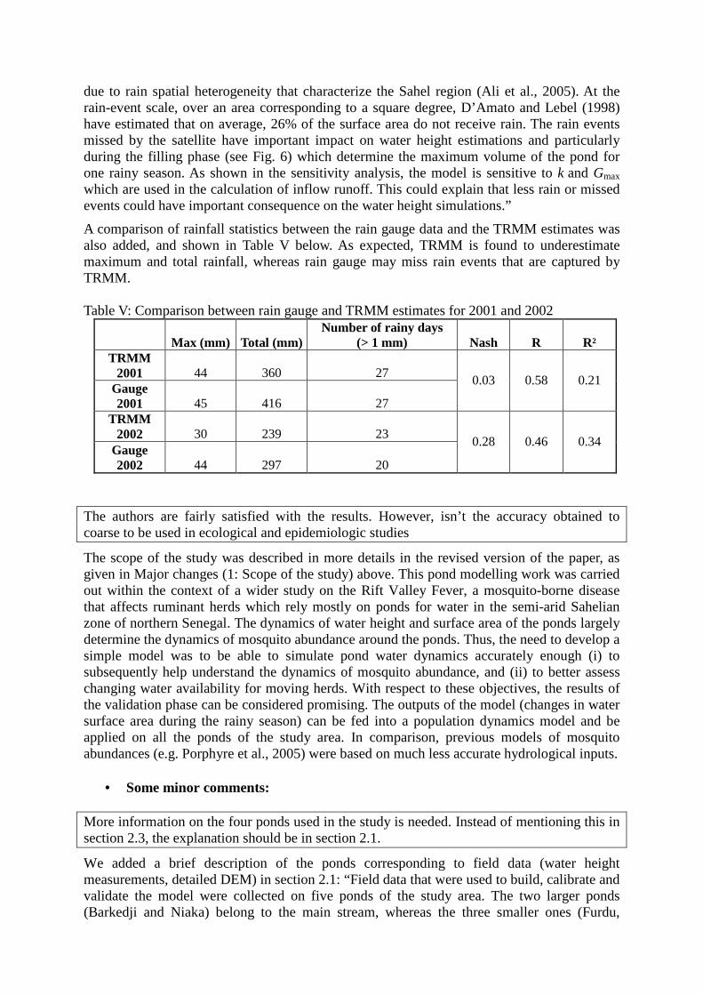
due to rain spatial heterogeneity that characterize the Sahel region (Ali et al., 2005). At the rain-event scale, over an area corresponding to a square degree, D’Amato and Lebel (1998) have estimated that on average, 26% of the surface area do not receive rain. The rain events missed by the satellite have important impact on water height estimations and particularly during the filling phase (see Fig. 6) which determine the maximum volume of the pond for one rainy season. As shown in the sensitivity analysis, the model is sensitive to k and Gmax which are used in the calculation of inflow runoff. This could explain that less rain or missed events could have important consequence on the water height simulations.”

A comparison of rainfall statistics between the rain gauge data and the TRMM estimates was also added, and shown in Table V below. As expected, TRMM is found to underestimate maximum and total rainfall, whereas rain gauge may miss rain events that are captured by TRMM. Table V: Comparison between rain gauge and TRMM estimates for 2001 and 2002

Max (mm) Total (mm) Number of rainy days

(> 1 mm) Nash R R² TRMM

2001 44 360 27 Gauge 2001 45 416 27

0.03 0.58 0.21

TRMM 2002 30 239 23

Gauge 2002 44 297 20

0.28 0.46 0.34

The authors are fairly satisfied with the results. However, isn’t the accuracy obtained to coarse to be used in ecological and epidemiologic studies

The scope of the study was described in more details in the revised version of the paper, as given in Major changes (1: Scope of the study) above. This pond modelling work was carried out within the context of a wider study on the Rift Valley Fever, a mosquito-borne disease that affects ruminant herds which rely mostly on ponds for water in the semi-arid Sahelian zone of northern Senegal. The dynamics of water height and surface area of the ponds largely determine the dynamics of mosquito abundance around the ponds. Thus, the need to develop a simple model was to be able to simulate pond water dynamics accurately enough (i) to subsequently help understand the dynamics of mosquito abundance, and (ii) to better assess changing water availability for moving herds. With respect to these objectives, the results of the validation phase can be considered promising. The outputs of the model (changes in water surface area during the rainy season) can be fed into a population dynamics model and be applied on all the ponds of the study area. In comparison, previous models of mosquito abundances (e.g. Porphyre et al., 2005) were based on much less accurate hydrological inputs.

• Some minor comments: More information on the four ponds used in the study is needed. Instead of mentioning this in section 2.3, the explanation should be in section 2.1.

We added a brief description of the ponds corresponding to field data (water height measurements, detailed DEM) in section 2.1: “Field data that were used to build, calibrate and validate the model were collected on five ponds of the study area. The two larger ponds (Barkedji and Niaka) belong to the main stream, whereas the three smaller ones (Furdu,

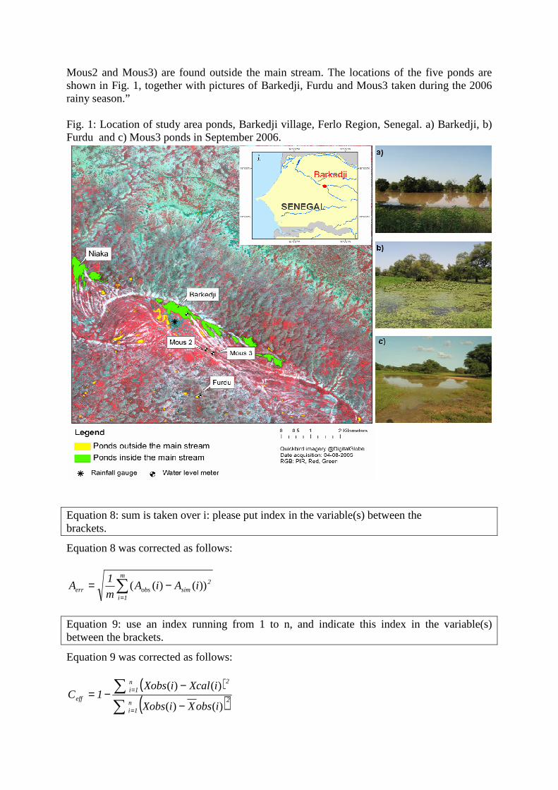
Mous2 and Mous3) are found outside the main stream. The locations of the five ponds are shown in Fig. 1, together with pictures of Barkedji, Furdu and Mous3 taken during the 2006 rainy season.” Fig. 1: Location of study area ponds, Barkedji village, Ferlo Region, Senegal. a) Barkedji, b) Furdu and c) Mous3 ponds in September 2006.

Equation 8: sum is taken over i: please put index in the variable(s) between the brackets.

Equation 8 was corrected as follows:

2sim

m

1iobserr iAiA

m

1A ))()(( −= ∑

=

Equation 9: use an index running from 1 to n, and indicate this index in the variable(s) between the brackets.

Equation 9 was corrected as follows:

( )( )2n

1i

2n1i

eff

iobsXiXobs

iXcaliXobs1C

)()(

)()(

−

−−=∑∑

=

=

In Table 2, the runoff coefficient is indicated in %, however, it should read 0:15 <Kr < 0:40.

“15 <Kr < 40” was replaced by “0.15 <Kr < 0.40” In Table 2, k should be unitless.

Right. Appropriate units have now been included in Table 2. Given the doubts on the hydrological model, the assumptions on the robustness of the model parameters and the very brief discussion of the results, I believe this paper is not ready to publish but should undergo additional research.

A major revision of the paper has now been carried out to take all the comments, corrections and suggestions of the four Referees into account. And in the process, we believe the paper has been significantly improved and should be considered for publication in HESS.