Chapter 2Review of Hough Transform for Line Detection

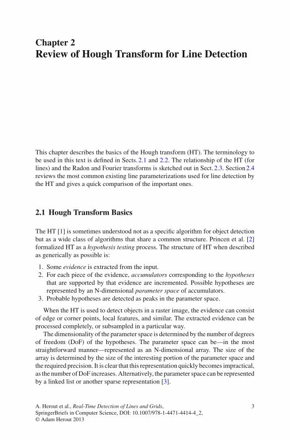
This chapter describes the basics of the Hough transform (HT). The terminology tobe used in this text is defined in Sects. 2.1 and 2.2. The relationship of the HT (forlines) and the Radon and Fourier transforms is sketched out in Sect. 2.3. Section 2.4reviews the most common existing line parameterizations used for line detection bythe HT and gives a quick comparison of the important ones.

2.1 Hough Transform Basics

The HT [1] is sometimes understood not as a specific algorithm for object detectionbut as a wide class of algorithms that share a common structure. Princen et al. [2]formalized HT as a hypothesis testing process. The structure of HT when describedas generically as possible is:

1. Some evidence is extracted from the input.2. For each piece of the evidence, accumulators corresponding to the hypotheses

that are supported by that evidence are incremented. Possible hypotheses arerepresented by an N-dimensional parameter space of accumulators.

3. Probable hypotheses are detected as peaks in the parameter space.

When the HT is used to detect objects in a raster image, the evidence can consistof edge or corner points, local features, and similar. The extracted evidence can beprocessed completely, or subsampled in a particular way.

The dimensionality of the parameter space is determined by the number of degreesof freedom (DoF) of the hypotheses. The parameter space can be—in the moststraightforward manner—represented as an N-dimensional array. The size of thearray is determined by the size of the interesting portion of the parameter space andthe required precision. It is clear that this representation quickly becomes impractical,as the number of DoF increases. Alternatively, the parameter space can be representedby a linked list or another sparse representation [3].

A. Herout et al., Real-Time Detection of Lines and Grids, 3SpringerBriefs in Computer Science, DOI: 10.1007/978-1-4471-4414-4_2,© Adam Herout 2013

4 2 Review of Hough Transform for Line Detection

The accumulation of the evidence can also be viewed as voting. Usually, onepiece of evidence affects many hypotheses but only a small portion of the parameterspace. The accumulator for each hypothesis is usually (and in the original Hough’sform of the transformation) integer, i.e., each piece of the evidence either does ordoes not support a given hypothesis. However, several variations of HT use fractionalaccumulators, so that the hypotheses can be supported only partially. Such methodsmodel the parameter space by fuzzy [4] or probabilistic [5] ways or perform somesort of antialiasing [6].

2.2 HT Formalization for 2D Curves

HT is typically used for detecting curves with an analytical description. In that case,the evidence are edge points detected in the input raster image. Such edge points cantypically be detected by gradient operators such as Sobel or Prewitt. The hypothesesare the possible curves of a given class in the image. For example, a line has two anda circle has three DoF in a 2D space, but HT can be used for detection of objectssuch as hyperspheres or hyperplanes in spaces of arbitrary dimensionality.

If a family of (2D) curves is specified by an implicit function

f (x, y, p1, . . . , pN ) = 0, (2.1)

where x and y are the image space coordinates and values p1, . . . , pN the parame-ter space coordinates, a point (x, y) that lies on a curve specifies a portion of theparameter space that describes all curves passing through this point. The parameterspace coordinates and their mapping to the curve specify the parameterization of thecurve. Curves typically have many possible parameterizations. It is always possibleto use a different base if the curve parameters form a vector space, but often, manyparameterizations fundamentally different in their nature are usable. Algorithm 1describes the detection of a curve specified by Eq. (2.1).

In many cases, the edge points are detected by a detector that can estimate theedge orientation (e.g., the Sobel operator). The edge orientation can then be usedto reduce the amount of curves that are plausible for the given edge point. Onlythe accumulators for curves whose tangent direction is close to the direction of thedetected edge are incremented. This technique was used by O’Gorman and Clowes [7]to speed up line detection, but it can be used for a wider variety of curves. Various fastHT implementations described in Chaps. 3 and 6 utilize this technique for speedingup the accumulation process.

Shapes that do not have a simple analytical description can be detected by usingthe Generalized HT by Ballard [8]. In GHT, the object is not described by an equationbut by a set of contour elements (edge points). Each contour element is describedby its position with respect to the object reference point and the edge orientation.The parameter space has a dimension from two to four (object position, orientation,

2.2 HT Formalization for 2D Curves 5

Algorithm 1 Implicit curve detection by Hough Transform.Input: Input image I , size of parameter space HOutput: Detected curves C

PI = {(x, y)|(x, y) are coordinates of a pixel in I}PH = {(p1, . . . , pN )|(p1, . . . , pN ) are coordinates in H}H(x)← 0,∀x ∈ PHfor all x ∈ PI do

if at x is an edge in I thenfor all {p : p ∈ PH , f (x, p) = 0} do

H(p)← H(p)+ 1end for

end ifend forC = {p|p ∈ PH , at p is a high local maximum in H}

and scale), but the representation of the detected object is complex even for simpleshapes.

The shapes for the GHT can also be expressed by random forests [9]. This rep-resentation improves the performance for some kinds of objects. The Hough forestsand the HT in general are the alternative of the object detection by a scanning windowclassifier.

2.3 Hough Transform for Lines and its Relationship to theRadon and Fourier Transform

The HT was originally developed for detecting lines and it is still popular in thisparticular area. Therefore, a large amount of different line parameterizations andvarious algorithmic modifications exist. Because 2D lines are rank 1 polynomialfunctions and therefore have two DoF, all line parameterizations are two dimensional.For now, a line will be specified by its normal vector n = (nx , ny) and the distancefrom the origin �. Every point p = (px , py) that lies on the line fulfills

p · n = �. (2.2)

HT for line detection is closely related to the Radon Transform [10, 11]. In thecontinuous case, these two transforms are identical. They differ in the discrete case,but some of the properties of the Radon transform are still applicable and useful.S.R. Deans [11] examined the properties of the Radon transform of a line segment,a pixel, and a generic curve.

The Radon Transform in an N -dimensional space transforms a functionf : R

N → R onto its integrals over hyperplanes. A point p lies on a hyperplane

6 2 Review of Hough Transform for Line Detection

(n, �) iff (if and only if) p · n = �. The function f must vanish to zero outsideof some area around the origin. Otherwise, the value of the line integral would beinfinite.

Equation (2.3) differs from the HT structure (Sect. 2.1) in the order of the iteration.The HT iterates over the affected hypotheses for every piece of the evidence so it isbuilding the whole parameter space at once. The RT finds the amount of evidencefor a given hypothesis by iterating over the evidence, so it tests every hypothesisseparately.

RN [ f ](n, �) =∫

RN

f (x)δ(x · n − �)dx

=∫

x·n=�

f (x)dx (2.3)

=∫

n⊥

f (�n + x)dx

Through the relation to the Radon Transform, the HT is also related to the FourierTransform. One- and N-dimensional versions of the Fourier transform are

F1[ f ](ξ) =∞∫

−∞f (x)e−2π i xξ dx, (2.4)

F N [ f ](w) =∫

RN

f (x)e−2π i(x·w)dx. (2.5)

The transforms are related via the Projection-Slice theorem [10], where the Radontransform is the projection part. One-dimensional Fourier transform of the Radontransform is equal to a slice of the N-dimensional Fourier transform along the direc-tion specified by the hyperplane’s normal vector. Notation

RN [ f ](n, �) = RNn [ f ](�) (2.6)

will be used. The relation between Radon and Fourier transform is then

F1[RNn [ f ]](ξ) = F N [ f ](ξn). (2.7)

Due to this relation, 2D convolution in the image space can be transformed to 1Dconvolution in the parameter space as

RNn [ f ∗ g](�) = (RN

n [ f ] ∗RNn [g])(�). (2.8)

2.3 Hough Transform for Lines and its Relationship to the Radon and Fourier Transform 7

The proof can be found in the work of Natterer [10]. This feature can be used notonly for image filtering, but it also generalizes the technique Han et al. used forcalculation of the α-cut in the Fuzzy HT [4].

Moving the filtering from the image to the parameter space can be beneficial notonly because of the lower computational cost. For example, some filtering methodscan interfere with the edge detection and moving the filtering after the voting step(to the voting space) allows for filtering without disturbing the edge detection phase.

2.4 Line Parameterizations

Usage of the HT for line parameterization requires a point transformation to theHough space. The motivation for introducing new parameterizations is to find theoptimal trade-off between requirements for the transformation. These requirementsinclude preference of bounding Hough space, discretization with minimal aliasingerrors, and uniform distribution of discretization error or intuitive mapping fromoriginal system to the Hough space. In general, the image of a point can be a curveof different shapes; for example circle, sinusoid curve, straight line, etc.

A subset favoring intuitive mapping and very fast line rasterization is the set ofpoint-to-line mappings (PTLM). It contains such parameterizations where a point inthe source image corresponds to a line in the Hough space and—naturally for theHT—a point in the Hough space represents a line in the x-y image space. PTLMwere studied by Bhattacharya et al. [12], who proved that for a single PTLM, theHough space must be infinite. However, for many PTLMs, a complementary PTLMcan be found, so that the two mappings define two finite Hough spaces containing alllines possible in the bounded image. An example is the original HT (Eq. 2.14) whichuses one Hough space for the vertical lines and the second one for the horizontallines.

The following text will first present transformations based on ‘classic’ line para-meterizations and the representations of these parameters. The second half belongsto the parameterizations using values of intersections of the line and a boundingobject. At the end of this section, a comparison of the mentioned parameterizationsis made, focusing on utilization of the Hough space and its main characteristics.

Slope–Intercept ParameterizationThe first HT, introduced and patented by Paul Hough in 1962 [1], was based on theline equation in the slope-intercept form. However, the exact line equation is notmentioned in the patent itself. Commonly, the slope-intercept line equation has theform:

� : y = xm + b, (2.9)

but the method used in the Hough’s patent corresponds to the parameterization:

� : x = ym + b. (2.10)

8 2 Review of Hough Transform for Line Detection

Fig. 2.1: Hough transform using m–b and k–q parameterizations of a line. Left inputimage; right corresponding Hough space

Using parameters m and b, all lines passing through a single point form a line inthe Hough space, so it is a PTLM. As in every PTLM, the parameter space of allpossible lines in a bounded input image is infinite [12]. Using a bounded parameterspace requires at least two complementary spaces of parameters. In the case of theslope–intercept line equation, these spaces are, for example, the two based on theseequations (Fig. 2.1):

y = xm + b,

x = yk + q.(2.11)

The slope–intercept parameterization is one of the parameterizations that allowsfor moving the image convolution to the parameter space as shown in Sect. 2.3.Contrary to Eq. (2.8), some scaling is necessary.

Hm[ f ∗ g](b) = 1√1+ m2

(Hm[ f ] ∗Hm[g])(b). (2.12)

Cascaded Hough TransformTuytelaars et al. [13] added a third space and used this three-fold parameterization

to detect the vanishing points and the horizon. This modification, named CascadedHough Transform, uses three pairs of parameters based on Eq. (2.13).

ax + b + y = 0 (2.13)

The three subspaces are created as shown in Fig. 2.2. The first one has coordinatesa−b, the second (1/a)−(b/a), and the third (1/b)−(a/b). All spaces are restrictedto the interval [−1, 1] in both directions. Each point (x, y) in the original spaceis transformed into a line in each of the three subspaces. Moreover, even in an

2.4 Line Parameterizations 9

b/a

b/1a/1

a/b

b

a

AB C

D

E F

B

A

B

CD

FE

A B

D

x

y

E

C

F

Fig. 2.2: Cascaded Hough transform using three spaces. Left-top input image; Rightand Bottom corresponding Hough spaces

unbounded image plane, every line corresponds to a point with coordinates withinarea [−1, 1] × [−1, 1] for one of the spaces (see Fig. 2.2).

Consider the input image scaled to get image boundaries±1. The significant partof the third subspace is without any vote and just the first two subspaces are neededto represent all lines from the image. However, CHT is mainly used for vanishingpoints and line detection, where the third space is indispensable. For more details,please see [13, 14].

θ − � parameterizationIn 1972, Duda and Hart [15] introduced a very popular parameterization denoted

as θ − � which is very important for its inherently bounded parameter space. It isbased on the line equation in the normal form (2.14)

y sin θ + x cos θ = �, (2.14)

10 2 Review of Hough Transform for Line Detection

A

B

C

θ

ρ

π/2 πx

y

ρθ

A

B

C

Fig. 2.3: Hough transform using θ − � parameterization of line. Left input space;right corresponding Hough space

where parameter θ represents the angle of inclination and� is the length of the shortestchord between the line and the origin of the image coordinate system (Fig. 2.3 left).In this case, images of all lines passing through a single point form a sinusoid curvein the parameter space (Fig. 2.3 right). Hence, θ−� is not a PTLM and for a boundedinput image it has a bounded parameter space.

For the θ − � parameterization, Eq. (2.8) can be used without any modification.Therefore, an image convolution (filtering) can be done by a 1D convolution of theHough space of image f with kernel g as

Hθ [ f ∗ g](�) = (Hθ [ f ] ∗Hθ [g])(�). (2.15)

Circle TransformSimilar to the θ − ρ parameterization, the circle transform [16] uses the normal

equation of the line (2.14). However, instead of the θ and ρ parameters it uses theintersection of the line and its normal passing through the origin O . This point fullycharacterizes a line. From the other side, points corresponding to all possible linespassing through an arbitrary point create a circle (see Fig. 2.4), i.e., point P is by theCT transformed into circle c. The center of the circle c is the midpoint between Oand P and the radius is equal to one-half of the distance |O P| (Eq. 2.16).

P = (a, b)E2 = (ρ cos θ, ρ sin θ)

c : x = 1

2(ρ cos θ + Ox ) (2.16)

y = 1

2(ρ sin θ + Oy)

The problem of such accumulation is that at the origin and very close to it, thenumber of votes is much higher than in the rest of the accumulator space. It is because

2.4 Line Parameterizations 11

A

B

C

x

y

x

y

A

BC

Fig. 2.4: Circle transform using θ–� parameterization of line. Left input space; rightcorresponding Hough space

A

B

C

d2

d1

x

y

A

B

C

d1

h

d2

w

w

h+w

h+2w

w h+w h+2w 2h+2w

Fig. 2.5: Muff Transform. A line is parameterized by its intersections with the bound-ing rectangle

all circles pass through the origin by definition. The possible solution is to put theorigin outside of the input image. However, the usage of the second space is neededbecause some line representations can now also lie outside of the input image.

Muff TransformSeveral research groups invested effort to find other bounded parameterizations

suitable for the HT. One of them is the Muff-transform introduced by Wallace in1985 [17] (Fig. 2.5). As the basis for this parameterization, a bounding rectanglearound the image is used. Each line intersects the bounding box at exactly two points.The distance of the first intersection (i.e. the nearest intersection from the origin alongthe perimeter) on the perimeter from the origin, and the distance between the firstand the second intersections are used as the parameters.

12 2 Review of Hough Transform for Line Detection

A

B

C

x

y

AB

C

αϕ

ϕ

α

π/2

π

2ππ

A

Fig. 2.6: Fan-Beam Transform. Line is parametrized by its orientation and intersec-tion with the bounding circle

The main advantages are the bounded Hough space and the discretization errorconnected directly to the discretization of the input image; thus, it is possible torepresent all necessary values as integers. The problem is the very sparse usage of theHough space. However, this can be eliminated by rearrangement of the componentsof the accumulator space. Also, the curve accumulated to the space has discontinuitiescaused by corners of the bounding rectangle.

Fan–Beam ParameterizationUsing a circle instead of a rectangle defines another bounded parameterization,

called the fan–beam parameterization [10] (Fig. 2.6). Again, a line and a circleintersect at exactly two points. Angles defined by these two points were used for aline parameterization for the first time by Eckhardt and Maderlechner [18].

Similar to Muff transform, the parameters belong to the original image plane whichmakes the discretization intuitive. In contrast, the accumulated line is smooth, andthe aliasing error is thus minimized. The accumulator, again, needs rearrangementfor optimal utilization of the memory.

Forman TransformThe Muff transform is also a basis for a parameterization introduced by

Forman [19], who combined it with θ−� and represented lines by the first intersectionpoint and the line’s orientation θ (Fig. 2.7).

2.4.1 A Quick Comparison of Selected Line Parameterizations

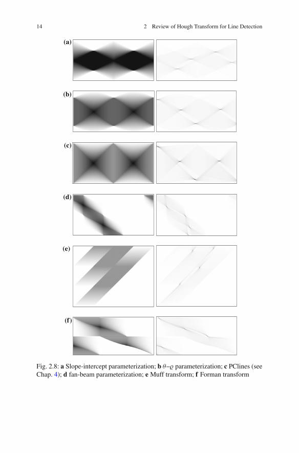
Different line parameterizations offer advantages and each one of them has its costs.One important aspect of the parameterizations’ properties is the uniformity of sam-pling of the voting space. The behavior of different parameterizations is illustratedby images in Fig. 2.8.

2.4 Line Parameterizations 13

A

B

C

d

x

y

A

BC

d

h

w

w h+w h+2w

θ

θ

π/2

π

Fig. 2.7: Forman’s parameterization based on θ–� and Muff Transform

Figure 2.8 shows the utilization of the Hough space for different parameterizationsin a manner similar to the work of Mejdani et al. [20]. The Hough space is accumulatedfor a 128 × 128 square image with each point considered as an edge point foraccumulation (left column) and for an image with four lines (right column). Themore the votes are accumulated, the darker the color is used. Always, the point witha maximal number of votes has absolutely black color and the point with the lowestvalue is white. Between these values, the color is linearly interpolated depending onthe number of votes.

It should be noted that each parameterization can have an accumulator space alittle bit different for different implementations, for example when the origin is inthe center of the input image or in its corner. Some of the parameterizations have theaccumulator space composed from several subspaces, which also enables a betterarrangement for optimal utilization of computer memory. However, the arrangementused in Fig. 2.8 is sufficient for the illustration and corresponds to Figs. 2.1–2.7.

From the rasterized Hough spaces, several characteristic aspects can be observed.The main is the utilization of the accumulator (Table 2.1). The best utilization hasthe PClines parameterization (Chap. 4); on the other hand, the largest unused partshas the Fan beam transform. The second is the distribution of the votes and thenumber of bins with the maximal value. In an ideal case, one bin in the accumulatorspace corresponds to one line in the input image. This implies that the maximum ofthe votes has to be equal to the length (number of pixels) of the longest line in theimage. Such a line is the diagonal and it occurs two times in the rectangular shape.That means two bins with maximal votes. A higher number of maximal bins, forexample in the slope-intercept parameterization, indicates the presence of aliasingerrors caused by discretization.

Different transformations also vary in the rasterized and accumulated shape inthe Hough space. From computational aspect, the fastest is accumulation of lines.However, as mentioned at the beginning of this section and proved in [12], all PTLMneed at least two twin spaces. This causes discontinuities and (dis)favors lines with

14 2 Review of Hough Transform for Line Detection

(a)

(b)

(c)

(d)

(e)

(f)

Fig. 2.8: a Slope-intercept parameterization; b θ–� parameterization; c PClines (seeChap. 4); d fan-beam parameterization; e Muff transform; f Forman transform

2.4 Line Parameterizations 15

Table 2.1: Basic characteristics of the selected transformations

Parameterization Utilization (%) Image of a point Space components

slope–intercept Slope–intercept 75 Lines 2θ − � Inclination–distance 89 Sinusoid curve 1Cascaded Slope–intercept – Lines 3Circle Inclination–distance – Circle 2PClines xy coordinate 100 Lines 1Muff Bounding rectangle 50 Curve 6Fan–beam Bounding circle 36 Curve 1Forman Inclination–distance 63 Curve 1

Bounding box

The first column reflects the used parameters/values; the second is the fraction of the bins fromthe Hough space where at least one vote is present; the third is the shape of the image of a pointafter mapping; and the last is the number of components in which the Hough space can be dividedcanonically

specific orientations. For example, when using the θ − � transformation, a pointis mapped to a smooth sinusoid curve and the discretization error is distributeduniformly through the whole Hough space. On the other hand, a PTLM slope–intercept parameterization prefers diagonal lines over horizontal and vertical (formore information about the discretization error, please see Sect. 4.3). The types ofpoint images for different parameterizations are concluded in Table 2.1.

The last property shown in Table 2.1 is the number of components of the Houghspace. This reflects the number of subspaces required, for example, from the defi-nition of the PTLMs. The value also serves as information of discontinuity of thewhole space. The higher the number is, the more the joints are in the space whichimplies more discontinuities.

References

1. Hough, P.V.C.: Method and means for recognizing complex patterns. U.S. Patent 3,069,654,1962

2. Princen, J., Illingowrth, J., Kittler, J.: Hypothesis testing: a framework for analyzing and opti-mizing Hough transform performance. IEEE Trans. Pattern Anal. Mach. Intell. 16(4), 329–341(1994). http://dx.doi.org/10.1109/34.277588

3. Kälviäinen, H., Hirvonen, P., Xu, L., Oja, E.: Probabilistic and non-probabilisticHough transforms: overview and comparisons. Image Vis. Comput. 13(4), 239–252(1995). doi:10.1016/0262-8856(95)99713-B, http://www.sciencedirect.com/science/article/pii/026288569599713B

4. Han, J.H., Kóczy, L.T., Poston, T.: Fuzzy Hough transform. Pattern Recogn. Lett. 15,649–658 (1994). doi:10.1016/0167-8655(94)90068-X, http://dl.acm.org/citation.cfm?id=189757.189759

5. Stephens, R.: Probabilistic approach to the Hough transform. Image Vis. Comput. 9(1),66–71 (1991). doi:10.1016/0262-8856(91)90051-P, http://www.sciencedirect.com/science/article/pii/026288569190051P

16 2 Review of Hough Transform for Line Detection

6. Kiryati, N., Bruckstein, A.: Antialiasing the Hough transform. CVGIP Graph. ModelsImage Process. 53(3), 213–222 (1991). doi:10.1016/1049-9652(91)90043-J, http://www.sciencedirect.com/science/article/pii/104996529190043J

7. O’Gorman, F., Clowes, M.B.: Finding picture edges through collinearity of feature points.IEEE Trans. Comput. 25(4), 449–456 (1976)

8. Ballard, D.H.: Generalizing the Hough transform to detect arbitrary shapes. Pattern Recogn.13(2), 111–122 (1981)

9. Gall, J., Yao, A., Razavi, N., Gool, L.V., Lempitsky, V.: Hough forests for object detection,tracking, and action recognition. IEEE Trans. Pattern Anal. Mach. Intell. 33, 2188–2202 (2011).http://doi.ieeecomputersociety.org/10.1109/TPAMI.2011.70

10. Natterer, F.: The Mathematics of Computerized Tomography. Wiley, New York (1986)11. Deans, S.R.: Hough transform from the radon transform. IEEE Trans. Pattern Anal. Mach.

Intell. PAMI-3(2), 185–188 (1981). doi:10.1109/TPAMI.1981.476707612. Bhattacharya, P., Rosenfeld, A., Weiss, I.: Point-to-line mappings as Hough transforms. Pattern

Recogn. Lett. 23(14), 1705–1710 (2002). http://dx.doi.org/10.1016/S0167-8655(02)00133-213. Tuytelaars, T., Proesmans, M., Gool, L.V., Mi, E.: The cascaded hough transform. In: Proceed-

ings of ICIP, pp. 736–739 (1997)14. Tuytelaars, T., Proesmans, M., Gool, L.V.: The cascaded Hough transform as support for

grouping and finding vanishing points and lines. In: Proceedings of the International Workshopon Algebraic Frames for the Perception-Action Cycle, AFPAC ’97, pp. 278–289. Springer,London, UK (1997). http://dl.acm.org/citation.cfm?id=646049.677093

15. Duda, R.O., Hart, P.E.: Use of the Hough transformation to detect lines and curves in pictures.Commun. ACM 15(1), 11–15 (1972). http://doi.acm.org/10.1145/361237.361242

16. Sewisy, A.A.: Graphical techniques for detecting lines with the hough transform. Int. J. Comput.Math. 79(1), 49–64 (2002). doi:10.1080/00207160211911, http://www.tandfonline.com/doi/abs/10.1080/00207160211911

17. Wallace, R.: A modified Hough transform for lines. In: Proceedings of CVPR 1985, pp. 665–667(1985)

18. Eckhardt, U., Maderlechner, G.: Application of the projected Hough transform in pictureprocessing. In: Proceedings of the 4th International Conference on Pattern Recognition, pp.370–379. Springer, London, UK (1988)

19. Forman, A.V.: A modified Hough transform for detecting lines in digital imagery. Appl. Artif.Intell. III, 151–160 (1986)

20. El Mejdani, S., Egli, R., Dubeau, F.: Old and new straight-line detectors: description andcomparison. Pattern Recogn. 41, 1845–1866 (2008). doi:10.1016/j.patcog.2007.11.013, http://dl.acm.org/citation.cfm?id=1343128.1343451

http://www.springer.com/978-1-4471-4413-7