review notes on microeconomic theory, bc version · pdf filereview notes on microeconomic...

Review Notes on Microeconomic Theory, BC Version

David Schenck Wills Hickman

October 10, 2012; version 0.0.6

Abstract

A very quick review of first-year microeconomic theory, specifically for BC’s Ec740-741.Schenck was responsible for sections 054. Hickman wrote section 6.

Brief Contents

0 Introduction 4

1 Decision Theory under Certainty 5

2 General Equilibrium Theory 12

3 Decision Theory Under Uncertainty 15

4 The Theory of Social Choice 19

5 Game Theory 21

6 Game Theory Subject Index 24

1

Contents

0 Introduction 4

1 Decision Theory under Certainty 51.1 Preferences and Utility . . . . . . . . . . . . . . . . . . . . . . . . . . . . . . . . . . . 51.2 Utility Maximization Problem . . . . . . . . . . . . . . . . . . . . . . . . . . . . . . . 61.3 Expenditure Minimization Problem . . . . . . . . . . . . . . . . . . . . . . . . . . . . 61.4 Identities, Slutsky, Comparative Statics . . . . . . . . . . . . . . . . . . . . . . . . . 71.5 The labor-leisure model . . . . . . . . . . . . . . . . . . . . . . . . . . . . . . . . . . 91.6 Individual Welfare . . . . . . . . . . . . . . . . . . . . . . . . . . . . . . . . . . . . . 101.7 Reprise . . . . . . . . . . . . . . . . . . . . . . . . . . . . . . . . . . . . . . . . . . . 10

2 General Equilibrium Theory 122.1 Robinson Crusoe . . . . . . . . . . . . . . . . . . . . . . . . . . . . . . . . . . . . . . 132.2 An Endowment Economy . . . . . . . . . . . . . . . . . . . . . . . . . . . . . . . . . 132.3 More on Existence . . . . . . . . . . . . . . . . . . . . . . . . . . . . . . . . . . . . . 142.4 Miscellaneous Topics . . . . . . . . . . . . . . . . . . . . . . . . . . . . . . . . . . . . 142.5 Production Economies . . . . . . . . . . . . . . . . . . . . . . . . . . . . . . . . . . . 142.6 Applications and Market Failure . . . . . . . . . . . . . . . . . . . . . . . . . . . . . 142.7 Uncertainty . . . . . . . . . . . . . . . . . . . . . . . . . . . . . . . . . . . . . . . . . 142.8 The 2x2 Model of Production . . . . . . . . . . . . . . . . . . . . . . . . . . . . . . . 142.9 Theory of the Second Best . . . . . . . . . . . . . . . . . . . . . . . . . . . . . . . . . 14

3 Decision Theory Under Uncertainty 153.1 Preferences and Utilty, again . . . . . . . . . . . . . . . . . . . . . . . . . . . . . . . 153.2 Risk Aversion . . . . . . . . . . . . . . . . . . . . . . . . . . . . . . . . . . . . . . . . 163.3 Portfolio Choice . . . . . . . . . . . . . . . . . . . . . . . . . . . . . . . . . . . . . . . 163.4 Insurance . . . . . . . . . . . . . . . . . . . . . . . . . . . . . . . . . . . . . . . . . . 173.5 Stochastic Dominance . . . . . . . . . . . . . . . . . . . . . . . . . . . . . . . . . . . 17

4 The Theory of Social Choice 194.1 Arrow’s Theorem . . . . . . . . . . . . . . . . . . . . . . . . . . . . . . . . . . . . . . 194.2 Generalizations of Arrow . . . . . . . . . . . . . . . . . . . . . . . . . . . . . . . . . . 204.3 Harsanyi’s Utilitarianism . . . . . . . . . . . . . . . . . . . . . . . . . . . . . . . . . . 20

5 Game Theory 215.1 Perfect Information Static Games . . . . . . . . . . . . . . . . . . . . . . . . . . . . . 215.2 Perfect Information Dynamic Games . . . . . . . . . . . . . . . . . . . . . . . . . . . 215.3 Bayesian Static Games . . . . . . . . . . . . . . . . . . . . . . . . . . . . . . . . . . . 215.4 Bayesian Dynamic Games . . . . . . . . . . . . . . . . . . . . . . . . . . . . . . . . . 215.5 Information Economics . . . . . . . . . . . . . . . . . . . . . . . . . . . . . . . . . . . 235.6 Mechanism Design . . . . . . . . . . . . . . . . . . . . . . . . . . . . . . . . . . . . . 235.7 Repeated Games . . . . . . . . . . . . . . . . . . . . . . . . . . . . . . . . . . . . . . 23

2

6 Game Theory Subject Index 246.1 Strategic Games . . . . . . . . . . . . . . . . . . . . . . . . . . . . . . . . . . . . . . 246.2 Solutions Through Common Knowledge of Rationality . . . . . . . . . . . . . . . . . 246.3 Extensive-Form Games with Perfect Information . . . . . . . . . . . . . . . . . . . . 256.4 Strategic Games with Imperfect Information . . . . . . . . . . . . . . . . . . . . . . . 256.5 Extensive Form Games . . . . . . . . . . . . . . . . . . . . . . . . . . . . . . . . . . . 256.6 Information Economics . . . . . . . . . . . . . . . . . . . . . . . . . . . . . . . . . . . 266.7 Mechanism Theory . . . . . . . . . . . . . . . . . . . . . . . . . . . . . . . . . . . . . 276.8 Dominant Strategy Mechanism Design . . . . . . . . . . . . . . . . . . . . . . . . . . 286.9 Repeated Games . . . . . . . . . . . . . . . . . . . . . . . . . . . . . . . . . . . . . . 29

3

0 Introduction

Section 1 consumer choice theory in the context of Kraus’ module. It covers the canonical modelof the consumer, the labor-leisure model, and welfare applications.

Section 2 investigates general equilibrium theory, Konishi’s module. My review notes follow thelecture notes he provided. (still incomplete)

Sections 3 and 4 address decision theory under uncertainty and social choice theory, Segal’smodule. I have rearranged the material in a manner I find more logical.

The final section discusses game theory, Unver’s module.

4

1 Decision Theory under Certainty

1.1 Preferences and Utility

The consumer’s basic problem is to choose the bundle that maximises her satisfaction from amongthe feasible set of bundles. I introduce two primitive concepts:

1. X is the “choice space”. It consists of all feasible bundles of goods.

2. � is the “at least as preferred to” relation, given by:

(a) a � a, the relation is reflexive;

(b) either a � b or b � a or both; the relation is complete;

(c) if a � b and b � c then a � c; the relation is transitive.

Similarly define �, ∼, ≺, �.

The consumer’s choice problem is then formally:

choose x ∈ X s.t. x � y ∀y ∈ X (1)

It is indeed possible to do all of microeconomics using the at least as preferred relation overchoice sets; however, this gets cumbersome quickly if the choice set is large. So instead of workingwith the at least as preferred relation, we need to put some mathematical clothing on the problemso that we can apply results of optimization theory.

For the canonical problem, let X = Rn+ where n is the number of distinct commodities and theposition in the ith position is the amount of good i being consumed. For now we do not put anyfurther restrictions on the choice set. Let’s put some more structure on �.

1. Continuity: For all y in X, the sets {x : x � y} and {x : x � y} are closed.

2. Strong monotonicity: if y vector dominates x, then y � x.

3. Strict convexity: given x 6= y and z in X, if x � z and y � z then tx + (1 − t)y � z for all0 ≤ t ≤ 1.

Define a utilty function u(x) as a mapping from an arbitrary x ∈ X to a number on the realline. A natural question is whether there exists such a function that represents the preferences �;that is, u(x) ≥ u(y) if and only if x � y. Does such a rationalization necessarily exist?

In general, the answer is no. It is possible to construct creative enough preference relationsthat one cannot perform this rationalization. Lexicographic preferences, for example, cannot berationalized by a utility function. However, for many of the interesting problems in economics it ispossible to rationalize the � relation into a utility function.

Suppose preferences are complete, reflexive, transitive, continuous, and stronglymonotonic. Then there exists a continuous utility function which represents thosepreferences. That is, u(x) ≥ u(y) iff x � y. The proof is in Varian.

So we have transitioned from (X,�) to u(x). u(x) is incredibly useful: it is a function u :Rn → R, and in particular can be shown to be continuous in its arguments. That means we canapply the powerful tools of differential calculus and optimization to our consumer’s choice problem,instead of working through weakly-preferred-to notation. We now define the feasible set. Supposethe consumer has cash endowment m and let pi be the cash price of good xi. Then the constrainedchoice set C is simply {x : px ≤ I}.

Properties of the utility function:

5

1. given (R, T, C, Continuity, and SM), there exists a u(x) represents �: u(x) ≥ u(y) iff x � y.

2. u is unique up to an increasing transformation. If v(·) is an increasing function and u(x)represents �, then v(u(x)) represents �. Anoher way of saying this is that utility is ordinal,not cardinal.

3. If � satisfies convexity, then u is quasiconcave.

1.2 Utility Maximization Problem

The consumer’s problem is now:

maxx

u(x) s.t. px = m (2)

L(x, λ) = u(x)− λ[px−m]

with p being prices and m money income. The consumer is assumed to know the price vector,and be a price-taker. The solution to this problem yields a vector of demand correspondencesx(p,m). The structure we have put on the problem yields the results that:

1. x(p,m) is homogenous of degree 0 in (p,m).

2. if u(x) is strictly concave, then x(p,m) is a function (rather than a correspondence)

Now plug the demand functions back into the utility function to obtain the indirect utilityfunction v(p,m) ≡ u(x(p,m)). This function has the following properties:

1. v(p,m) is nonincreasing in p. (Higher prices make you no better off and probably worse off)

2. v(p,m) is nondecreasing in m. (More income cannot make you worse off and probably makeyou better off)

3. v(p,m) is quasiconvex in p.

4. Roy’s Identity: xi(p,m) = −Div(p,m)/Dmv(p,m)

1.3 Expenditure Minimization Problem

Alternatively, we could set up the consumer’s problem in another way: find the minimum expen-diture needed to obtain a certain level of utility U . Formally,

minxp · x s.t. u(x) = U (3)

L(x, µ) = px− µ[u(x)− U ]

Solve this problem and you’re left with a vector of equations h(p, U). These are the “Hicks” or“compensated” demand functions. A change in price is “compensated” to keep the consumer onthe same indifference curve.

The Hicks demand curves have the following properties:

1. H.D.0 in p

2. the matrix (∂hi/∂pj) is negative semidefinite

Plug the h(p, U) functions into the maximand to obtain e(p, U) = p · h(p, U). Now the expen-diture function e(p, U) has the following properties:

6

1. HD1 in p

2. increasing in U

3. nondecreasing in p

4. concave in p

5. Shephard’s Lemma.

We have defined now the four basic analytic elements of consumer theory under certainty:the Marshallean demand curve, the indirect utilty function, the Hicks demand curve, and theexpenditure function.

1.4 Identities, Slutsky, Comparative Statics

Linking Identities

We now search for ways to link the preceeding four concepts. I provide:

1. Roy’s Identity: −∂v(p,m)∂pi

/∂v(p,m)∂m ≡ xi(p,m)

2. Shephard’s Lemma: ∂e(p,U)∂pi

≡ hi(p, U)

3. e(p, v(p,m)) ≡ m

4. v(p, e(p, u)) ≡ u

The Roy and Shephard identities link the indirect utility function and expenditure functionto their respective demand functions; each is a direct application of the Envelope Theorem. Thesecond pair of identities link the indirect utility function and expenditure function to each other:importantly, at the optimal point (x∗, u∗,m∗) the two are identical.

Substitution Matrix

S =

D1(h1(p, u)) D2(h1(p, u)) . . . Dn(h1(p, U))D1(h2(p, u)) D2(h2(p, u)) . . . Dn(h2(p, u))

. . . . . . . . . . . .D1(hn(p, u)) D2(hn(p, u)) . . . Dn(hn(p, u))

that is, the matrix of derivatives of the h(p, u) vector with respect to each price. This is the so-calledsubstitution matrix and may be written compactly as

S = (sij) = (hij)

by which we mean the ith derivative of the jth Hicks demand function. Each function gets arow; alternatively each price derivative gets a column. The substitution matrix has the followingproperties:

1. It is the Hessian of the expenditure function

2. it is negative semidefinite (follows from the concavity of e(p, U))

3. it is symmetric (and hence the (i,j) subscripts may be inverted)

7

4. own-price effects must be negative

5. the sum of substitution effects is zero; i.e. columns and rows must sum to zero.

6. Given the previous two points, there must exist at least one Hicks substitute (a good withpositive cross-substitution effects)

Slutsky identity

Next consider the relationship between the slope of the ordinary demand function x(p,m) and theHickesan demand function h(p, U). In particular we have the following identity:

∂xj(p,m)

∂pi=∂hj(p, U

∗)

∂pi− ∂xj(p,m)

∂mxi(p,m)

where U∗ = v(p,m). Simply: the derivative of the ordinary demand function consists of a substi-tution and income effect and is additively separable into the two. Derivation:

hj(p, U) = xj(p, e(p, U))

∂hj(p, U)

∂pi=∂xj(p, e(p, U))

∂pi+∂xj(p, e(p, U))

∂e(p, U)

∂e(p, U)

∂pi∂hj∂pi

=∂xj∂pi

+∂xj∂m

hj(p, U)

∂hj∂pi

=∂xj∂pi

+∂xj∂m

xj(p,m)

=⇒ ∂xj∂pi

=∂hj∂pi− ∂xj∂m

xj(p,m)

which is the desired expression.

Comparative Statics

We now investigate the comparative static exercise more formally. For simplicity focus on thetwo-good case. I present the method in stepwise format.

Set up the problem:

L(x1, x2, λ) = [u(x1, x2)]− λ[p1x1 + p2x2 −m].

Given appropriate smoothness and concavity conditions, the solution is necessarily and sufficientlygiven by the the FOC. So the first step is to set up the necessary conditions:

u1 − λp1!

= 0

u2 − λp2!

= 0

m− p1x1 − p2x2!

= 0

This is precisely a vector of FOCs: u1 − λp1u2 − λp2

m− p1x1 − p2x2

=

000

8

Totally differentiate the vector of FOC’s. The resulting object is a matrix called the Jacobian: u11 u12 −p1u21 u22 −p2−p1 −p2 0

dx1dx2dλ

+

−λ 0 00 −λ 0−x1 −x2 1

dp1dp2dm

= 0

Note that the first matrix is simply the Hessian of the Lagrangian with respect to the choicevariables. The second matrix is the coefficient matrix for the exogenous variables, p1, p2 and m.Rearrange: u11 u12 −p1

u21 u22 −p2−p1 −p2 0

dx1dx2dλ

=

λ 0 00 λ 0x1 x2 −1

dp1dp2dm

finally, assuming that the Hessian of the Lagrangian is invertible, dx1

dx2dλ

=

u11 u12 −p1u21 u22 −p2−p1 −p2 0

−1 λ 0 00 λ 0x1 x2 −1

dp1dp2dm

(4)

Now the relevant partial derivatives may be read off directly as entries of the coefficient matrix.

1.5 The labor-leisure model

Suppose now the endowment is not money but time. The consumer has a time endowment T aswell as an autonomus money endowment m. The consumer works h hours and uses the remainingl hours as leisure. Utility is granted by leisure and the consumption good c. Formally,

maxc,l

u(c, l) s.t. pc = wh+m

h+ l = T

We can combine the two constraints into a single constraint:

maxc,l

u(c, l) s.t. pc = w(T − l) +m (5)

L(c, l, µ) = [u(c, l)]− µ[pc+ wl − wT −m]

First-order conditions:

L1 = u1(c, l)− µp!

= 0

L2 = u2(c, l)− µw!

= 0

Lµ = pc+ wl!

= wT +m

From here we may solve as usual. The trick is to write down the constraints (time, money, etc)separately, then find some way to combine them into a single aggregate constraint.

9

1.6 Individual Welfare

Finally, we consider the effect of price and income changes on consumer welfare. We define theequivalent variation and compensating variation as:

EV ≡ e(p0, U1)− e(p0, U0) (6)

CV ≡ e(p1, U1)− e(p1, U0) (7)

The EV is a measure of the change in expenditure needed to achieve utility U1 from U0 underconstant prices p0. The CV is a measure of the change in expenditure needed to achieve utility U1

from U0 under constant prices p1.CV and EV can also be thought of as the area under a Hicksean demand curve in the special

case where only one price is changing. That is,

EV =

∫ p01

p11

h(p1, p, U1)dp1

CV =

∫ p01

p11

h(p1, p, U0)dp1

Finally, the consumer surplus is the area under the ordinary demand curve from p0 to p1:

CS ≡∫ p01

p11

x(p1, p,m)dp1

CS, EV and CV are equivalent under the demand curves induced by quasilinear preferences. Oth-wewise, under a price reduction, EV ¿ CS ¿ CV for normal goods. Note that EV and CV areunobservable, being dependent on utility, but CS is observable. In addition, it can be shown thatthe error introduced by using CS instead of CV/EV is rather small.

1.7 Reprise

The basic ideas of Kraus’ module may be related in the following picture:

10

(X,�)

u(x),x ∈ Rn+

max u(x)s.t.

px ≤ m

min pxs.t.

u(x) = U

x(p,m) h(p, U)

v(p,m) =u(x(p,m))

e(p, U) =ph(p, U)

(sij)

EV, CVSlutsky

eqn

ConsumerSurplus

(dxidpj

)

existence theorem

Lagrangian

plug inRoy

Identity

Identity

Lagrangian

plug inShephard

take derivatives

Hessian

welfare

Duality

The red column is the utility maximization problem; the blue column is the expenditure mini-mization problem. Applications of the two are labelled accordingly.

11

2 General Equilibrium Theory

Definitions

Let X1 ≡ (x11, x12, . . . , x

1k) be an allocation of goods given to person 1.

Let X ≡ (X1, . . . Xn) be a collection of such individual allocations.

Definition 1. Walras’ Law: Suppose the consumer is optimizing and suppose local nonsatiation.Then for every price vector p, p · z(p) = 0.

In general, p · z(p) ≤ 0.

Definition 2. A core allocation is a feasible allocation X such that for all nonempty subgroupsof consumers S ⊆ I, there is no feasible re-allocation for S that makes at least one person in Sbetter off.

Definition 3. An allocation is Pareto efficient if there is no way to rearrange resources such thatat least one person is better off, and no person is worse off. The set of Pareto efficient allocationsis the Pareto set.

Definition 4. A core allocation is a Walrasian equilibrium if it is supported by a price p.

Result: Walrasian Equilibria ⊆ Core ⊆ Pareto set

12

2.1 Robinson Crusoe

This is the simplest possible general equilibrium economy. Setup:

1. there is one consumer who maximizes u(c, 1− n).

2. there is one production technology, f(n).

3. the consumer owns the technology.

It’s a natural extension of the labor-leisure model.The consumer solves:

maxc,n

u(c, 1− n) s.t. c ≤ wn+ π (8)

=⇒ L(c, n, λ) = [u(c, 1− n)]− λ[c− wn− π]

where c is consumption, n is labor, w the real wage, and π exogenous dividend income. Timeendowment is normalized to unity. FOC are

u1(c, 1− n) = λ

u2(c, 1− n) = λw

c = wn+ π

Rearrange these three equations to obtain the labor supply curve, ns = n(w, π) and the consumptiondemand curve, c = c(w, π).

The firm solves

maxn

f(n)− wn (9)

which yields n = n(w), the labor demand curve (equivalently the FOC is w = f ′(n), the inverselabor demand curve). Finally, dividends are given by π = f(n∗)− w∗n∗.

In equilibirum we have c = f(n), all output is consumed. Three consumer FOCs, the firm FOC,the dividend equation, and the adding-up condition are enough to solve the problem.

Endogenous are consumption c, labor n, the multiplier λ, the wage w and profits π. Thefirm FOC gives a labor demand curve, the consumer gives a labor supply curve, and the dividendequation jointly determine n, w, and π. Then one can use n to determine f(n) = y, y = c, andfinally one can find the multiplier λ.

2.2 An Endowment Economy

Now consider the case of two goods and two consumers. Each consumer wishes to:

maxx1,x2

u(x1, x2) s.t. p1x1 + p2x2 = p1ω1 + p2ω2

where ω’s are endowments. As usual only relative prices matter; we can normalize any one priceto unity. Prices are taken as given by each consumer but will be solved for in equilibrium.

We can graphically analyze the problem with an Edgeworth box:

13

O1

O2

x1

x2

x2

x1

ω

O1 is the origin for agent 1, O2 is the origin for agent 2. The width of the box is the sum of x1endowments; the height is the sum of x2 endowments. The point ω is the endowment point.

2.3 More on Existence

2.4 Miscellaneous Topics

2.5 Production Economies

2.6 Applications and Market Failure

2.7 Uncertainty

2.8 The 2x2 Model of Production

2.9 Theory of the Second Best

14

3 Decision Theory Under Uncertainty

3.1 Preferences and Utilty, again

Recall the consumer choice framework under certainty. We assumed that the objects of interestwere bundles of commodities, x ∈ X, with X a subset of RN+ .. We assumed that � was defined overcommodity bundles and satisfied reflexivity, completeness, transitivity, continuity, strictmonotonicity, and strict convexity. We need a little more structure to analyze choice underuncertainty.

The objects of interest are no longer commodity bundles, but lotteries over the set of commodi-ties. Formalizing the problem, let X be the set of all commodities under consideration. X mightbe finite or infinite, but suppose for now that it’s finite. Let ∆ be the set of probabilities: eachelement is nonnegative and the sum of the elements exactly equals unity. The object of study is∆(X), the set of all possible probabilities over the choice options. The best way to think of X is asa set of money outcomes, and ∆ as probabilities for those money outcomes.

Assume the consumer has preferences � over lotteries. Since X is fixed, a “lottery” is simply alist of probabilities, one for each outcome in X. Suppose that in the set of lotteries, there exists amost preferred lottery b and a least preferred lottery w. This assumption is not strictly necessarybut makes the math much easier.

Notation: let X be the set of outcomes; X,Y, Z ∈ ∆(X) be lotteries; and x ∈ X be a singleoutcome. A lottery X over (x, y, z) is denoted X ≡ (x, px; y, py; z, pz). Formally lotteries X aresimply random variables.

Suppose:

1. Reflexivity: if X ∈ ∆(X), then X � X.

2. Completeness: X � Y or Y � X or both, but not neither

3. Transitivity: X � Y and Y � Z implies X � Z.

4. Continuity: for all x ∈ X, there exists a p such that: (x, 1) ∼ (b, p;w, (1− p)).

5. Independence. Let X,Y, Z ∈ ∆(X). Then:(X, 1) � (Y, 1) iff (X, p;Z, (1−p)) � (Y, p;Z, (1−p)). That is, adding an irrelevant alternative(with the same probability on both sides) does not change one’s preference.

6. Reduction: in a compound lottery, the consumer only cares about final probabilities.

The first three are identical to the certainty case. The fourth is an uncertainty analogue tocontinuity in the certainty case. Independence is new, and so is reduction.

Next, define the expected utility function over lotteries eu(X) as:

eu(X) =

n∑i=1

piu(xi). (10)

Let’s break this down a little and see what’s going on. Suppose our consumer has the certaintyutility function u(x) over the outcomes in X. Now suppose that we pick a lottery X. Then theconsumer’s expected utility from the lottery X is simply the expected value of the utility of theindividual outcomes. Note carefully that there is no index on u(·); the utility function over certainoutcomes is fixed (unique up to a positive affine transformation). That is, there is an “underlying”utility function over the set of outcomes.

15

The expected utility form is extremely useful. Can it be rationalized? In general, no, but formany of the scenarios of interest to economists, yes it can. Suppose the � relation satisfies R,C, T, Continuity, Independence, and Reduction. Then there exists an expected utilityfunction eu(X) representing �.

Properties of the eu(X) function:

1. it is unique up to an affine transformation. Let eu(x) =∑piu(xi) represent � and let

v(θ) = aθ + b. Then∑piv(u(xi)) also represents �. This is more restrictive than our old

definition, wherein any monotonic v could represent the same � as u.

2. eu(X) is increasing and continuous.

The fundamental consumer choice problem is to pick the best lottery available to him, not thebest outcome. He maximizes the expected utility of the lottery.

3.2 Risk Aversion

A decision-maker is said to be risk-averse if she finds u(E[X], 1) preferable to eu(X). Consider thecase where there are two outcomes, x1 and x2. Then we are saying that

u(px1 + (1− p)x2) ≥ pu(x1) + (1− p)u(x2)

But this is precisely the definition of a concave function. Thus we arrive at the main result, that adecision-maker is risk averse iff her utility function is concave.

Risk aversion comes with a few associated definitions:

CE[X] = x : X ∼ (CE[X], 1)

π[X] = E[X]− CE[X]

RA(x) = −u′′(x)

u′(x)

RR(x) = −xu′′(x)

u′(x)

CE[X] is the certainty equivalent of X; it is the dollar value that makes the decision-maker indif-ferent from receiving the dollar value and playing the lottery. Typically the CE[X] is less than theexpected value of X.

The risk premium π[X] is the difference between the expected value of a lottery and its certaintyequivalent.

The final two equations are measures of absolute and relative risk aversion.

3.3 Portfolio Choice

We now apply the material on lotteries to portfolio allocation. Suppose the decision maker hasinitial wealth w to be split into two categories: a risky asset a and a riskless asset m. Normalizeso that the rate of return on m is unity, and let a be a lottery X = (x1, p1; . . . ;xn, pn). The firstquestion is whether the DM will put money into the risky asset at all. We have the following result:a > 0 ⇐⇒ E[X] > 0.

Decreasing absolute risk aversion implies da/dw > 0. As income rises, the amount invested inthe risky asset rises.

Increasing absolute risk aversion implies d( aw )/dw < 0.

16

3.4 Insurance

Suppose there are two events, E and ¬E. E occurs with probability p. Suppose initial wealth isw and he faces a possible loss of L. The price of one dollar of insurance is q. That is, the DMgets one dollar if E happens, and nothing if E does not happen. The DM is choosing how muchinsurance to buy, X.

If he buys X dollars of insurance, he will face the lottery

(w − qX − L+X, p;w − qX, (1− p))

that is, if E happens he will obtain (wealth - cash spent on insurance - loss + insurance payout)and if ¬E happens he will obtain (wealth - cash spent on insurance). The expected utility of thelottery is

eu(X) = pu(w − qX − L+X) + (1− p)u(w − qX)

The optimal X satisfies

p(1− q)u′(w − qX − L+X)− q(1− p)u′(w − qX) = 0

When will the consumer buy full insurance? Whenever p(1 − q)u′(w − qL) = q(1 − p)u′(w − qL).That is, whenever p = q. Stated slightly differently, p = q implies full insurance.

Graphically, we have:

¬E

E

NI

FI

The 45 degree line is the “certainty case”. Points on that line occur regardless of whether E or¬E occurs. The slope of the NI − FI line is q/(1− q): it is a budget constraint.

As to the supply side, if there are competitive markets then suppliers will offer q = p. Inequilibrium, p = q, there are no profits, everybody buys full insurance, and the uncertainty isessentially traded away.

That’s if all people have equal probabilities. What of different probabilities? Separating equlib-rium.

3.5 Stochastic Dominance

We wish to have some measure as to whether one lottery is “better” than another, in the sense ofstrict monotonicity in certainty theory.

17

Let X, Y be lotteries. Let FX(t) be the cumulative distribution function of X; similarly FY (t).Then X dominates Y by first-order stochastic dominance if FX(t) < FY (t) for all t. Intuitively,FX is always “to the right of” FY , hence it is more desirable.

Again let X, Y be lotteries and let all outcomes line in [a, b]. X dominates Y by second-orderstochastic dominance if: ∫ x

aFX(t)dt ≤

∫ x

aFY (t)dt

for all x, and∫ ba FX(t)dt =

∫ ba FY (t)dt. The best way to think about this is in the context of

mean-preserving spreads. X SOSD Y if Y is a mean-preserving spread of X.

18

4 The Theory of Social Choice

4.1 Arrow’s Theorem

Define a “society” as: n ≥ 2 individuals and X set of social options, |X| ≥ 3. For each individual,let �i be defined over X. Furthermore denote society’s ranking as �, without a subscript. Hencesociety is a set (X,n, {�i}i=ni=1 ,�).

The individual �i relation is assumed to obey:

1. Complete: x � y or y � x or both, but not neither

2. Transitive: x � y and y � z implies x � z

3. Reflexive: x � x.

Note, in particular, that these are identical to the axioms we used in consumer choice undercertainty. Let X be finite so that an individual’s preference ordering is a vector from “best” to“worst”. Let a social profile be a list of such individual preferences; think of the profile as amatrix with each individual entering as a single column.

As an example, consider a society with 3 individuals and 3 social options, a, b, and c:

1 2 3

a b cb c ac a b

where we go down the columns to see how individuals rank options. Person 1 ranks a �1 b �1 c;person 2 ranks b �2 c �2 a; and person 3 ranks c �3 a �3 b. Note that in this example, we haveall the ingredients of a society except the social ranking. How should we organize the individualrankings into a group ranking? That is the first and fundamental problem of social choice.

We would like the social preference ordering to have the following properites:

1. Universal Domain: any profile may be admitted

2. Transitivity: if x � y and y � z then x � z.

3. Unanimity: if for all persons x �i y then societally, x � y.

4. Independence of Irrelevant Alternatives.

5. Non-Dictatorship

Universal Domain makes sense: we want our social rule to work no matter what the profiles are.Transitivity rules out cycles. Unanimity is a bare-minimum requirement: if everyone prefers x toy, we want society to prefer x to y as well. Think of it as a Pareto-type requirement. IIA is fine:we don’t want irrelevant options “on the ballot” to affect society’s choice of A against B. Now thisdoesn’t say that individuals can’t let C influence their A/B decision, only society cannot. Finally,non-dictatorship. Well. . .

Unfortunately we must begin with a sad result.

Theorem 1. Arrow’s Theorem. (UD, T, U, IIA, and ND) are mutually inconsistent

19

4.2 Generalizations of Arrow

So the five axioms are mutually inconsistent. One strain of the social choice literature tries tofind minimally-relaxed versions of Arrow’s axioms that generate positive results. We consider two:majority rule (which works) and Sen’s liberalism (which does not).

Majority Rule

Consider majority-rule voting. We know from the Condorcet paradox that in general, majority ruleis intransitive. However, if we relax UD we come across an important sub-class of preferences inwhich majority rule satisfies (U, T, IIA, and ND). That is, it satisfies all of Arrow’s axioms. Thisspecial case is for the class of single-peaked preferences. Formal political theory makes extensive(one might say exclusive) use of this case.

Formally,

Definition 5. Majority Rule: a � b iff |{a �i b}| > |{b �i a}|

Definition 6. Single peaked: preferences are single peaked if there exists a best option, and utilitydeclines monotonically to the left and right of the best option.

Theorem 2. Single-peaked implies optimality of majority rule. If preferences are single-peakedfor all i, then (UD, T, U, IIA, ND) are satisfied for majority rule.

Sen’s Liberalism

Suppose we replace IIA with the following: if two social options only affect some S ⊂ N , then ifall i ∈ S agree on the relative ranking of the two, then society will as well.

Unfortunately, this still yields intransitivity under some profiles.

4.3 Harsanyi’s Utilitarianism

Recall the expected utility model of the consumer. Now suppose all individuals in society followexpected utility theory, and that the social welfare function is also expressible as an expected utilityfunction. Then The social welfare function is a weighted average of individual utility functions.Formally:

Theorem 3. Harsanyi’s Utilitarianism. Suppose

1. Each individual’s preferences satisfy Eu theory

2. The social preference ordering satisfies Eu theory

3. Pareto: x �i y for all i and x �i y for some i implies x � y.

Then the social preferences over lotteries can be represented by

W (X) =∑

αiEui(X)

for some set of α.In particular, if X gives policy β with probability 1, then

W (β) =∑

αiui(β)

This is another powerful theorem: when we are concerned with actual social outcomes (certainlotteries), social welfare under that policy is a weighted average of individual welfare under thatpolicy.

20

5 Game Theory

5.1 Perfect Information Static Games

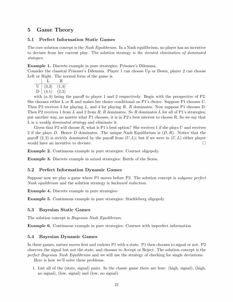
The core solution concept is the Nash Equilibrium. In a Nash equilibrium, no player has an incentiveto deviate from her current play. The solution strategy is the iterated elimination of dominatedstategies.

Example 1. Discrete example in pure strategies: Prisoner’s Dilemma.Consider the classical Prisoner’s Dilemma. Player 1 can choose Up or Down, player 2 can chooseLeft or Right. The normal form of the game is

L R

U (3,3) (1,4)D (4.1) (2,2)

with (a, b) being the payoff to player 1 and 2 respectively. Begin with the perspective of P2.She chooses either L or R and makes her choice conditional on P1’s choice. Suppose P1 chooses U.Then P2 receives 3 for playing L, and 4 for playing R. R dominates. Now suppose P1 chooses D.Then P2 receives 1 from L and 2 from R; R dominates. So R dominates L for all of P1’s strategies;put another way, no matter what P1 chooses, it is in P2’s best interest to choose R. So we say thatL is a weakly dominated strategy and eliminate it.

Given that P2 will choose R, what is P1’s best option? She receives 1 if she plays U and receives2 if she plays D. Hence D dominates. The unique Nash Equilibrium is (D,R). Notice that thepayoff (2, 2) is strictly dominated by the payoff from (U,L); but if we were in (U,L) either playerwould have an incentive to deviate.

Example 2. Continuous example in pure strategies: Cournot oligopoly.

Example 3. Discrete example in mixed strategies: Battle of the Sexes.

5.2 Perfect Information Dynamic Games

Suppose now we play a game where P1 moves before P2. The solution concept is subgame perfectNash equilibrium and the solution strategy is backward induction.

Example 4. Discrete example in pure strategies:

Example 5. Continuous example in pure strategies: Stackleberg oligopoly

5.3 Bayesian Static Games

The solution concept is Bayesian Nash Equilibrium.

Example 6. Continuous example in pure strategies: Cournot with imperfect information

5.4 Bayesian Dynamic Games

In these games, nature moves first and endows P1 with a state. P1 then chooses to signal or not. P2observes the signal but not the state, and chooses to Accept or Reject. The solution concept is theperfect Bayesian Nash Equilibrium and we will use the strategy of checking for single deviations.

Here is how we’ll solve these problems.

1. List all of the (state, signal) pairs. In the classic game there are four: (high, signal), (high,no signal), (low, signal) and (low, no signal).

21

2. The solution is either pooling or separated. In a pooling equilbrium both high types and lowtypes send the same signal (S or N). In a separating equilibrium different types send differentsignals (either HS, LN or HN, LS). Hence there are four equilibria.

3. Given pooling or separated, figure out what P2 will do. In a separating equilibrium, he willhave perfect info about agent types. In a pooling equilibrium, he will have no better infothan simply the prior distribution.

4. Check for single deviations.

• Suppose we have a separating equilibrium (HSA, LNR). Then “deviating” for a hightype is to choose N and be R. Is u(HNR) > u(HSA)? Then the equilibrium is notstable to single deviations. Similarly the “deviation” of the low type is to choose S andbe A. Is u(LSA) > u(LNR)? Then it’s not an equiibrium.

• Suppose we have a separating equilibrium (HN, LS). Same deal applies: “deviating”means (HS, LN) and being mistaken for the wrong type.

• Deviations from pooling equilibria are trickier and best done through example.

Example 7. Discrete example in pure strategies: Spence job market game

22

5.5 Information Economics

Here we are principally concerned with principal-agent problems.

5.6 Mechanism Design

5.7 Repeated Games

Example 8. Rubinstein/Baron division-of-the-dollar game.

Example 9. Iterated PD, forever and with stopping.

23

6 Game Theory Subject Index

6.1 Strategic Games

Idea of a Game: A game is a well-defined interaction with more than one decision maker, wherethe payoffs of the decision makers not only depend on their own decisions, rules of the game, andchance moves, but also on decisions of the other decision makers.A strategic game is a game in which each player chooses all of his actions, known as contingencyaction plans, once and for all at the beginning of the game.Define the following:

• Strategic(-form) Game / Normal Form Game

• Mixed Strategy

• Mixed Extension of a Game

• Nash Equilibrium

• Best Response Correspondence

State and prove the following theorems:

• Existence of Nash Equilibrium in Pure Strategies

• Existence of Nash Equilibrium in Mixed Strategies

Explain and or give specific examples of the following classical game types:

• Prisoner’s Dilemma

• Battle of the Sexes

• Cournot Oligopoly

Draw a diagram to illustrate the existence of mixed strategy equilibrium in a battle of the sexescontext.

6.2 Solutions Through Common Knowledge of Rationality

Explain knowledge and common knowledge in the context of game theory.Define the following:

• A Strictly (Weakly) Dominated Strategy

• Iterated Elimination of Strictly (Weakly) Dominated Strategies

Explain the following notation:

• MNE

• SNE

• SMNE

Prove the following theorems:

• SMNE ⊆ SIESDS

• If |SIESDS | = 1thenSIESDS ⊆ SNE .

24

6.3 Extensive-Form Games with Perfect Information

Explain/Define the following:

• Extensive-form Game with Perfect Information

• Strategic Games Induced by Extensive-form Games with Perfect Information

• NE of an Extensive-form Game with Perfect Information

• A Subgame of Extensive-form Game with P.I.

• Subgame Perfect Nash Equilibrium (SPE)

• Backward Induction

• Continuity of Payoffs at an Infinite History of an Infinite Horizon Extensive-form Game

• Rubinstein Bargaining Game

State (if necessary) and prove the following theorems:

• One Deviation Property

• Every finite-horizon extensive-form game with perfect information and infinite-horizon gamewith continuity of payoffs at infinity has a SPE in pure strategies.

• Existence of unique SPE in Rubinstein Bargaining Game


• Stackleberg Game

6.4 Strategic Games with Imperfect Information


• Bayesian Game

• Bayesian Nash Equilibrium (in pure strategies)


• First-Price Auction

6.5 Extensive Form Games

Define the following:

• Extensive Form Game

• Certainty/uncertainty in extensive form games

• Perfect Recall

• Perfect Information (for an extensive form game)

25

• Sequential Game

• Strategic-form Game in Extensive Form

• (mixed behavioral) Strategy

• Strategic Form Games Induced by Extensive Form Games

• Subgames (of Extensive Form Games)

• Sequentially Rational

• Assessment

• Belief system

• Perfect Bayesian Equilibrium

• Signaling Games

• Pooling PBE

• Separating PBE

• Intuitive Criterion

• A Consistent Assessment

• Sequential Equilibrium

How does one solve a game for each type of equilibrium?

6.6 Information Economics


• Adverse Selection

• Moral Hazard

• Single-Crossing Property

• The Principal-Agent Problem

Prove the following theorems:

• Let (ψl, ψh, s(.), µ(.)) be a perfect Bayesian equilibrium, where µ(B, p) is the equilibriumbelief of insurance company that at any proposed (B, p) the consumer is of low-risk type,s(B, p) is the action of the insurance company when face with offer (B, p), and let u∗l and u∗hdenote the equilibrium utility of the low- and high-risk consumer, respectively, given that shehas been chosen by Nature. Then

1. u∗l ≥ ul, and

2. u∗h ≥ uch

26

where ul ≡ max(B,p){ul (B, p) |p = πB} and uch ≡ uh(L, πL) denotes the high-risk consumer’sutility in the competitive equilibrium with full information.

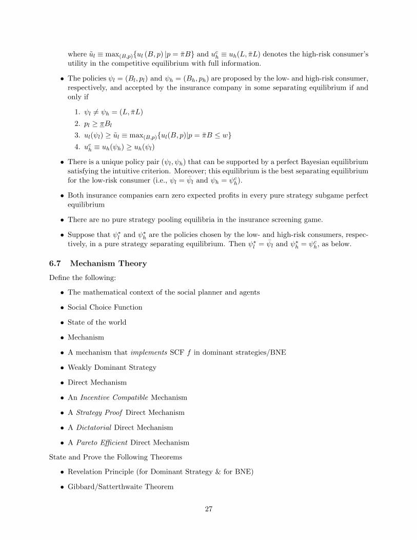
• The policies ψl = (Bl, pl) and ψh = (Bh, ph) are proposed by the low- and high-risk consumer,respectively, and accepted by the insurance company in some separating equilibrium if andonly if

1. ψl 6= ψh = (L, πL)

2. pl ≥ πBl3. ul(ψl) ≥ ul ≡ max(B,p){ul(B, p)|p = πB ≤ w}4. uch ≡ uh(ψh) ≥ uh(ψl)

• There is a unique policy pair (ψl, ψh) that can be supported by a perfect Bayesian equilibriumsatisfying the intuitive criterion. Moreover; this equilibrium is the best separating equilibriumfor the low-risk consumer (i.e., ψl = ψl and ψh = ψch).

• Both insurance companies earn zero expected profits in every pure strategy subgame perfectequilibrium

• There are no pure strategy pooling equilibria in the insurance screening game.

• Suppose that ψ∗l and ψ∗h are the policies chosen by the low- and high-risk consumers, respec-tively, in a pure strategy separating equilibrium. Then ψ∗l = ψl and ψ∗h = ψch, as below.

6.7 Mechanism Theory

Define the following:

• The mathematical context of the social planner and agents

• Social Choice Function

• State of the world

• Mechanism

• A mechanism that implements SCF f in dominant strategies/BNE

• Weakly Dominant Strategy

• Direct Mechanism

• An Incentive Compatible Mechanism

• A Strategy Proof Direct Mechanism

• A Dictatorial Direct Mechanism

• A Pareto Efficient Direct Mechanism

State and Prove the Following Theorems

• Revelation Principle (for Dominant Strategy & for BNE)

• Gibbard/Satterthwaite Theorem

27

6.8 Dominant Strategy Mechanism Design


• single-peaked preferences

• Median Voting Rule

• Phantom Voting Rules

• Social Decision

• Direct Mechanism

• An Efficient Decision Rule

• A Vickrey Auction

• Matching

• A Pareto Efficient Matching

• Mechanism

• Priority Mechanism

• A Neutral Mechanism

• A Non-Bossy Mechanism

State and prove the following:

• (Groves) Let d : T → A be an efficient decision rule and suppose that for each i there existsa function xi : Ti ≡ ×j 6=iTj → R such that

yi(t) = xi(t−i) +∑j 6=i

vj(tj , d(t)).

Then, (d, y) is a strategy-proof mechanism.

• (Green-Laffont) Conversely, let d : T → A be an efficient decision rule, (d, y) be a strategy-proof mechanism, and the type spaces be complete in the sense that {vi(ti, .) : D → R|ti ∈Ti} = {v : D → R}, the set of all possible value functions, for each i ∈ N . Then, for each ithere exists a function xi : T−i → R such that the transfer rule yi satisfies Equation 1.

• A priority mechanism is strategy-proof and Pareto-efficient in the house allocation domaindefined in the notes.

• A priority mechanism is non-bossy

• In the house allocation problem domain with strict preferences over houses, a mechanism iscoalitional strategy-proof if and only if it is non-bossy and strategy-proof.

Explain the following problems/games:

• Vickrey Auction

• House Allocation Problem

28

6.9 Repeated Games


• Stage Game

• Repeated Game with Public Information

• Average Discounted Payoff

• Average Feasible Payoff Graph

• Feasible Set of Average Payoffs

• Minmax Payoff of Player i in GT (δ)

• (Strictly) Individually Rational Payoff

Note: In what follows, PD2 refers to a prisoner’s dilemma with two NE in the stage game.Prove the following theorems:

• One Deviation Property

• (Benoit and Krishna 1985); two players, no discounting: Suppose (v′1, v

′2) and (v

′′1 , v

′′2 ) are

stage-game NE payoffs with v′1 < v

′′1 and v

′′2 < v

′2. For all pairs (v1, v2) feasible in the stage

game and greater than or equal to any convex combination of (v′1, v

′2) and (v

′′1 , v

′′2 ), there is a

finite repetition T such that GT′(1) with T

′ ≥ T has SPE with average payoffs within an εneighborhood of (v1, v2).

• Infinitely repeated PD2, discounted payoffs with δ > 12 : ”Grim Trigger” (meaning play C as

long as both play C, play D forever if any player ever plays D) is SPE and yields (C,C) forall times t.

– Note that if the punishment is not NE in the stage game then the repeated-game equi-librium is only NE, not SPE.

• Individual Rationality of NE: If (vi)i∈N is the average discounted payoff profile in a Nashequilibrium of GT (δ), then vi ≥ vi for all i.

• Nash Folk Theorem: If (vi)i∈N is a feasible and strictly individually rational payoff profile,then there exists δ < 1 such that for all δ ≥ δ, there is a NE of G∞(δ) with average payoffprofile (vi)i∈N .

• Subgame-perfect Folk Theorem: For any payoff profile (vi)i∈N that is strictly individuallyrational and feasible there exists δ < 1 such that for all δ ≥ δ, there is an SPE of G∞(δ) withaverage payoffs (vi)i∈N .

29

review notes on microeconomic theory, bc version · pdf filereview notes on microeconomic...

Documents