Gwt%ovascular Research

Cardiovascular Research 31 (1996) 371-379

Review

Linear and non-linear analyses of heart rate variability: a minireview

Pascale Mansier a* * , Jean Clairambault b, Nathalie Charlotte a, Claire Medigue b, Christophe Vermeiren b, Gilles LePape ‘, Fraqois Car& d, Athanassia Gounaropoulou a,

Bernard Swynghedauw a a UIZ7-INSERM, IFR Circulation, Hi?pital Lariboisike. 41 Bd de la Chapelle, 75010 Paris, France

b INRIA-Rocquencourt, Domine de Voluceau, BP 105.78153 Le Chesnay Cede& France ’ Laboratoire d’Ethologie et de Psychophysiologie. Faculte’ des Sciences et Techniques, Part de Grandmont, 37200 Tours, France

’ Luboratoire de Physiologie Midicale, Faculte’ de Midecine de Rennes, 2 -4 Au. du Pr. Leon Bernard, 35043 Rennes, France

Received 15 March 1995; accepted 20 October 1995

Abstract

To complete traditional time- and frequency-domain analyses, new methods derived from non-linear systems analysis have recently been developed for time series studies. A panel of the most widely used methods of heart rate analysis is given with computations on mouse data, before and after a single atropine injection.

Keywords: Linear analysis; Non-linear analysis; Heart rate variability

1. Introduction

Heart rate can be computed from an electrocardiogram (ECG): it is based on the RR series which represents the successive interbeat intervals. Within the same individual, important variations from the mean RR value are observed in every species studied, from man [l] (mean RR of 1 s) to mouse [2] (mean RR of 0.1 s). Heart rate variability (HRV) is defined as the fluctuations of the RR intervals around this mean value. HRV analysis assumes sinus rhythm and ectopic ventricular beats should be rejected. The influence of the Autonomic Nervous System (ANS) has long been recognized in these fluctuations, short-term variability be- ing mediated by the parasympathetic system, and long-term variability by both the sympathetic and parasympathetic pathways [3-71.

Epidemiological studies, beginning in the late seventies, have shown that a decrease in HRV is one of the best predictors of arrhythmic events or sudden death after myocardial infarction [8-131. Search for better methods of

* Corresponding author. Tel. (+33-l) 42-W-80-6.5; Fax (+33-l) 48. 74-23-15.

analysis has therefore more than an academic interest. HRV depends on various determinants including the baroreflex, cortical influences, but also, as recently sug- gested in our laboratory [1.5], the myocardial phenotype. The myocardial /3-adrenergic/muscarinic receptors ratio is modified during cardiac failure and experimental data have shown that these alterations parallel the decrease in HRV [ 14,151. To verify such a hypothesis, independently of any baroreflex influence, we have developed a model of trans- genie mice overexpressing P,-adrenergic receptors exclu- sively in atria [16]. Preliminary results reveal substantial alterations of sinus rhythm variability [2].

To illustrate a large panel of HRV analysis methods, we have purposely focussed our study on RR series obtained from the same young female mouse, before and after intraperitoneal (IP) injection of a single dose of atropine (100 mg/kg). Th e mouse is a model of growing interest because of the use of murine transgenic models in the cardiovascular domain [17-191. The ECGs were recorded by telemetry and the RR series were computed using DADISP software (DSP Development Corporation) and

Tie for primary review 21 days.

OOOS-6363/%/$15.00 0 1996 Elsevier Science B.V. PN SOOO8-6363(96)00009-O

312 P. Mazier et ul./Cardiovascular Research 31 (1996) 371-379

30 60 90 120 150 180

Time in s

“E

140

.f

a p:

120

0 30 60 90 120 150 180

Time in s

Fig. 1. Effects of atropine on heart rate in a mouse. A: control. B: after injection of a single dose of atropine (100 mg/kg). Tachograms. Heart rate recording uses a biocompatible ETA transmitter (DataSciences Inc, St Paul, MN, USA) via a telemetric device on a non-anaesthetized and freely moving young female mouse (4 months old; body weight 22.3 g). Sampling frequency: 3 kHz. Such a frequency ensures R wave detection with an accuracy < 1 ms. Signal digitized on a PC-based system (Axotape) and stored for further analysis on a Unix workstation. RR series were obtained from the ECG recordings using DADISP software and a level cross method to detect the R waves.

the effects of atropine injection are shown in Fig. 1A and B.

In the present review, methods of HRV analysis will be presented, derived from both classical signal processing and non-linear dynamics. The review will focus on a few points: (a) time-domain, spectral and time-frequency anal- yses are not exclusive of non-linear analysis; (b) the use of non-linear methods should not be restricted to proven deterministic chaos 1201; Cc) a rather large panel of meth- ods has to be used to provide reasonable evidence of chaotic, or at least non-linear, behaviour.

2. Methods of analysis of HRV

2.1. Spectral and non-spectral methods of analysis

Several articles have been published on this topic [4- 6,21,22] and this section is a review of some of the classical methods in use.

2.1.1. Time domain methods; Variability indexes Apart from the mean RR value, the effective calculation

of the standard deviation gives a coarse quantification of the variability, without distinguishing between short-term and long-term fluctuations. In our example, the heart rate of the mouse is round 500 bpm, with a mean RR value of 113 k 9 ms. Interestingly, atropine lowers the heart rate and increases the mean RR to 140 f 6 ms, instead of accelerating the heart rate as it does in most of the animal species, suggesting that mice have no vagal tone. Standard deviation was diminished from 9 to 6 ms. The calculation of the autocorrelation function is also instructive [correla- tion of the RR(i) with the RR(i + t), with varying t], which gives the standard deviation for t = 0. Furthermore, the autocorrelation function is periodic if the original series is periodic.

Many different variability indexes have been defined in various fields such as obstetrics [23] and cardiology [24] and some of them are widely used (Yeh’s indexes in obstetrics [23], and SDANN or SDNNSO [ 12,13,24] in cardiology). It is worth noting that most of the epidemio- logical studies demonstrating the prognostic value of a decrease in HRV after myocardial infarction have been based upon such indexes [ 131.

2.1.2. Frequency domain methods; Spectral analysis Spectral analysis consists in converting information in

the time domain into information in the frequency domain. The most widely used method for processing the studied signal is the Fast Fourier Transformation, PIT. The result of FIT is a complex number for each frequency; its squared modulus is the spectral power, and the set of all spectral powers for the different frequencies is the Power Spectral Density (PSD) function; its graph is the spectrum of the signal. Results are expressed in Power Spectral Density (PSD), the squared amplitude calculated for each frequency. The spectrum of the signal is the graph of the PSD function (y-axis) plotted against frequency (x-axis). Partitioning in High or Low Frequency variabilities, HF and LF, gives the short-term or long-term variability of the time series. The total HRV is obtained by calculating the total area under the PSD curve. Spectral analysis methods have been widely applied to both HRV and blood pressure variability. Nevertheless, spectral analysis presents intrin- sic limitations, especially in relation to the possible non- stationarity of the signals 1251. The FFT requires a station- ary signal: the statistical properties of the signal should be the same when their estimation is performed at different time intervals within the same recording. It also assumes that the recorded oscillations are symmetrical.

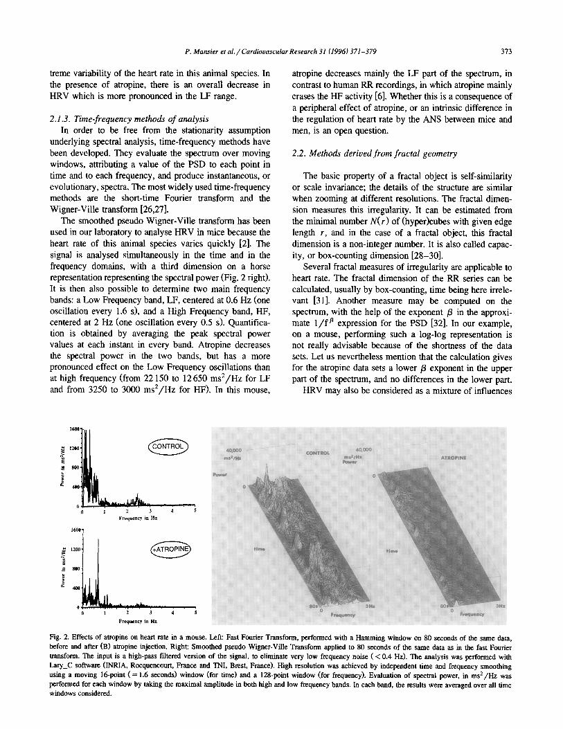
Fig. 2 (left) gives the result of a spectral analysis of the RR series performed by FIT using a Hamming window, and shows apparent activity in various frequency bands: a I-IF band around 2.4 Hz, a LF band around 0.6 Hz, and a very low frequency band below 0.4 Hz. The spectrum is complex, and the’quantification difficult due to the ex-

P. Mansier et al. / Cardiovascular Research 31 (1996) 371-379 373

treme variability of the heart rate in this animal species. In the presence of atropine, there is an overall decrease in HRV which is more pronounced in the LF range.

2.1.3. Time-jkequency methods of analysis In order to be free from the stationarity assumption

underlying spectral analysis, time-frequency methods have been developed. They evaluate the spectrum over moving windows, attributing a value of the PSD to each point in time and to each frequency, and produce instantaneous, or evolutionary, spectra. The most widely used time-frequency methods are the short-time Fourier transform and the Wigner-Ville transform [26,27].

The smoothed pseudo Wigner-Ville transform has been used in our laboratory to analyse HRV in mice because the heart rate of this animal species varies quickly [2]. The signal is analysed simultaneously in the time and in the frequency domains, with a third dimension on a horse representation representing the spectral power (Fig. 2 right). It is then also possible to determine two main frequency bands: a Low Frequency band, LF, centered at 0.6 Hz (one oscillation every 1.6 s), and a High Frequency band, HF, centered at 2 Hz (one oscillation every 0.5 s). Quantifica- tion is obtained by averaging the peak spectral power values at each instant in every band. Atropine decreases the spectral power in the two bands, but has a more pronounced effect on the Low Frequency oscillations than at high frequency (from 22 150 to 12 650 ms’/Hz for LF and from 3250 to 3000 ms*/Hz for I-IF). In this mouse,

N : mo

E .E so0 L D 2 4.0

0 n 1 3 4 5 ” -

Frequene? in Hz

.E aooi I

I:. 0 1 2 3 4 5

Frzquency in Hz

atropine decreases mainly the LF part of the spectrum, in contrast to human RR recordings, in which atropine mainly erases the I-IF activity [6]. Whether this is a consequence of a peripheral effect of atropine, or an intrinsic difference in the regulation of heart rate by the ANS between mice and men, is an open question.

2.2. Methods derived from fractal geometry

The basic property of a fractal object is self-similarity or scale invariance; the details of the structure are similar when zooming at different resolutions. The fractal dimen- sion measures this irregularity. It can be estimated from the minimal number N(r) of (hype&&es with given edge length r, and in the case of a fractal object, this fractal dimension is a non-integer number. It is also called capac- ity, or box-counting dimension [28-301.

Several fractal measures of irregularity are applicable to heart rate. The fractal dimension of the RR series can be calculated, usually by box-counting, time being here irrele- vant [311. Another measure may be computed on the spectrum, with the help of the exponent /3 in the approxi- mate l/f B expression for the PSD 1321. In our example, on a mouse, performing such a log-log representation is not really advisable because of the shortness of the data sets. Let us nevertheless mention that the calculation gives for the atropine data sets a lower /3 exponent in the upper part of the spectrum, and no differences in the lower part.

HRV may also be considered as a mixture of influences

Fig. 2. Effects of atropine on heart rate in a mouse. Left: Fast Fourier Transform, performed with a Hamming window on 80 seconds of the same data, before and after (B) atropine injection. Right: Smoothed pseudo Wigner-Ville Transform applied to 80 seconds of the same data as in the fast Fourier transform. The input is a high-pass filtered version of the signal, to eliminate very low frequency noise ( < 0.4 Hz). The analysis was performed with Lary-C software (INRIA, Rocquencourt, France and TNI, Brest, France). High resolution was achieved by independent time and frequency smoothing using a moving 16point ( = 1.6 seconds) window (for time) and a 12%point window (for frequency). Evaluation of spectral power, in ms2/Hz was performed for each window by taking the maximal amplitude in both high and low frequency bands. In each band, the results were averaged over all time windows considered.

314 P. Maker et al./Cardiovascular Research 31 (1996) 371-379

2- Dimension It& In - IQ- ISI-

Ml-

II-

IX-

Ill-

la-

w

CaO’ rl P) Pp la II7 IX If lM In 167 a IW 90 99 la II7 1% IIS ISI Iu I62 I71

3- Dimension

IN

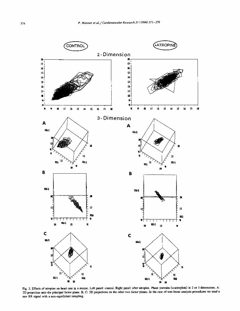
Fig. 3. Effects of atropine on heart rate in a mouse. Left panel: control. Right panel: after atropine. Phase portraits (scatterplots) in 2 or 3 dimensions. A: 2D projection onto the principal factor plane. B, C: 3D projections on the other two factor planes. In the case of non-linear analysis procedures we used a raw RR signal with a non-equidistant sampling.

P. Maker et al./Cardiovascular Research 31 (1996) 371-379 315

from the ANS (“harmonic component”) and a remaining “fractal component”: calculation will then consist in ex- tracting this fractal part of the HRV in the spectrum, computing its relative importance in the spectrum (fractal percentage) and determining a fractal exponent from the remaining part of the spectrum [33-351.

2.3. Methods of non-linear dynamics; Chaotic behaoiour

Sets of differential or difference equations describing the evolution of a system can display solutions that are totally unpredictable in the long run, because of “sensitive dependence on initial conditions”, even though the trajec- tories remain in a bounded region of the space. In other words, the divergence between two initially close trajecto- ries of the system is such that any estimation of the position of one point at a given time is impossible. And yet the system has nothing to do with chance: it is theoreti- cally determined by its equations and a starting point [36-391.

2.3.1. Attractors and chaos From a “dynamical” point of view, a discrete time

series, such as an RR series, is seen as the projection on a line of one trajectory of an unknown discrete deterministic dynamical system in m-dimensional space. If this evolu- tion is not subject to abrupt changes induced by external factors, such a trajectory will converge to an attractor, i.e. a closed set of points in m-dimensional space which is a limit set for all trajectories of the system, and one trajec- tory is supposed to cover the attractor if the time series is long enough. Many deterministic dynamical systems pre- sent attractors, but not all of them are chaotic. A chaotic attractor is defined by sensitive dependence on initial conditions for the trajectories on them; if, furthermore, it is a fractal object, with a non-integer dimension, then it is a strange attractor and displays no simple geometric struc- ture [40,41]. Chaos occurs only in non-linear systems. Widely known examples of strange attractors are H&on’s and Lorenz’s attractors [36-391.

2.3.2. The case of heart rate Application to biological systems is relatively new and

has been recently reviewed [42-441. The ECG may be viewed as a deterministic continuous dynamical system. The RR series is then considered as the sequence of “first return times” corresponding to the intersections of the trajectories with a fixed hyperplane, e.g. zero crossing for the action potential. In this respect, [RR, vs RR,, ,] plots, or [RR,, RR,, ,, RR n + 2 I plots [451 are not Poincare maps or first return maps but rather “first return time maps” of a continuous dynamical system; they are sometimes termed scatterplots [461, but the most widely used term is “phase portraits” [47]. Two- and three-dimensional phase portraits are shown in Fig. 3 for data obtained with a mouse. The control plots are geometrically ordered, in a cone-like

structure, whereas the atropine plots are distributed in a less ordered aspect.

2.3.3. Reconstructing a cardiac attractor from the RR series

Let us assume that a dynamical system of unknown dimension m underlies the RR series. Packard, Ruelle and Takens showed that one-dimensional projected data were sufficient to reconstruct an original m-dimensional attrac- tor with the method of delays [48]. It consists in consider- ing the time series (RR( t>, t = 1,2,...N], as the projection on one coordinate axis of an m-dimensional series {RR, = [RR(t), RR(t + T), RR(t + 271,. . . , RR(t + (m - l)~], t =12 , , . . . , N], taken as a trajectory on an attractor. As far as the RR series are concerned, a time lag T = 1 seems to be the most reasonable choice, since longer lags may induce undue loss of spatial correlation between points. The dimension m of the space in which one thus embeds the trajectory is called the embedding dimension. If it is chosen large enough (one should take m > 2 d, + 1 1481, where d, is the correlation dimension, see below), then the geometrical properties of the trajectory and of the recon- structed attractor are conserved by this processing. Statisti- cal and geometrical invariants of the attractor, such as dimension, Lyapunov exponents and entropy, may then be computed.

2.3.4. Measuring a cardiac attractor

2.3.4.1. Dimension. The dimension of an attractor can be given by the fractal dimension d, obtained by box-count- ing, the information dimension d, obtained by computing the information entropy, and the correlation dimension d, obtained by the Grassberger-Procaccia algorithm [49-5 11 or its variants [52]. If the experimental data are regularly distributed on the attractor, these three modes of calcula- tion give the same result. Such algorithms are limited by data length: 10d212 points are necessary to estimate di- mension d, [53]. For heart rate series, even a 24-h record- ing of heart rate (100 000 beats for a human heart, 700 000 beats for a mouse) cannot allow any estimation of the correlation dimension over 10. Furthermore, such a pro- cessing assumes that the attractor has not changed during the recording period. Such limitation in the length of data implies in particular that only low-dimensional chaos may be evidenced by dimension computation.

In the case of the mouse RR series, the atropine injec- tion induces an increase in the correlation dimension, regardless of the embedding dimension (Table 1) which clearly suggests that atropine enhances the “complexity” of the RR series (increased “complexity” simply meaning an increased dimension or number of degrees of freedom of a system). An embedding dimension of 3 is then apparently enough to estimate d,. In fact, we have also calculated d, for embedding dimensions up to 10, and have obtained a permanent decrease of d, after 5, instead

376 P. Maker et al./Curdiovascular Research 31 (1996) 371-379

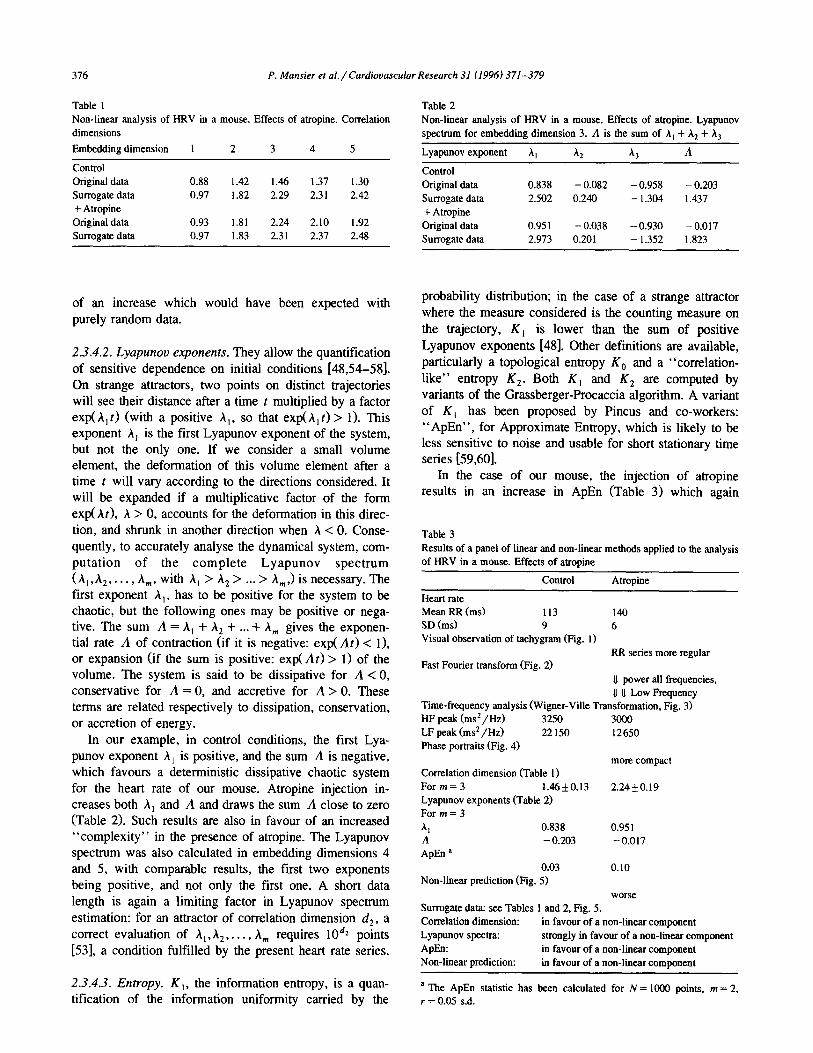
Non-linear analysis of HRV in a mouse. Effects of atropine. Correlation dimensions Embedding dimension 1 2 3 4 5

Control Original data 0.88 1.42 1.46 1.37 1.30 Surrogate data 0.97 1.82 2.29 2.31 2.42 + Atropine Original data 0.93 1.81 2.24 2.10 1.92 Surrogate data 0.97 1.83 2.3 1 2.37 2.48

Table 1 Table 2 Non-linear analysis of HRV in a mouse. Effects of atropine. Lyapunov spectrum for embedding dimension 3. A is the sum of A, + h, + h,

Lyapunov exponent A, A2 A3 A

Control Original data 0.838 - 0.082 - 0.958 - 0.203 Surrogate data 2.502 0.240 - 1.304 1.437 + Atropine Original data 0.95 1 - 0.038 - 0.930 -0.017 Surrogate data 2.913 0.201 - 1.352 1.823

of an increase which would have been expected with purely random data.

2.3.4.2. Lyupunou exponents. They allow the quantification of sensitive dependence on initial conditions [48,54-581. On strange attractors, two points on distinct trajectories will see their distance after a time t multiplied by a factor exp(A,t) (with a positive A,, so that exp(A,t)> 1). This exponent A, is the first Lyapunov exponent of the system, but not the only one. If we consider a small volume element, the deformation of this volume element after a time t will vary according to the directions considered. It will be expanded if a multiplicative factor of the form exp(ht), A > 0, accounts for the deformation in this direc- tion, and shrunk in another direction when A < 0. Conse- quently, to accurately analyse the dynamical system, com- putation of the complete Lyapunov spectrum (44 2,. . . , A,,,, with A, > A, > . . . > A,,,,) is necessary. The first exponent A,, has to be positive for the system to be chaotic, but the following ones may be positive or nega- tive. The sum A = A, + A, + . . . + A,,, gives the exponen- tial rate A of contraction (if it is negative: exp( Ar) < l), or expansion (if the sum is positive: exp( At) > 1) of the volume. The system is said to be dissipative for A < 0, conservative for A = 0, and accretive for A > 0. These terms are related respectively to dissipation, conservation, or accretion of energy.

probability distribution; in the case of a strange attractor where the measure considered is the counting measure on the trajectory, K, is lower than the sum of positive Lyapunov exponents [48]. Other definitions are available, particularly a topological entropy K, and a “correlation- like” entropy K,. Both K, and K, are computed by variants of the Grassberger-Procaccia algorithm. A variant of K, has been proposed by Pincus and co-workers: “ApEn”, for Approximate Entropy, which is likely to be less sensitive to noise and usable for short stationary time series [59,60].

In the case of our mouse, the injection of atropine results in an increase in ApEn (Table 3) which again

Table 3 Results of a panel of linear and non-linear methods applied to the analysis of HRV in a mouse. Effects of atropine

In our example, in control conditions, the first Lya- punov exponent A, is positive, and the sum A is negative, which favours a deterministic dissipative chaotic system for the heart rate of our mouse. Atropine injection in- creases both A, and A and draws the sum A close to zero (Table 2). Such results are also in favour of an increased “complexity” in the presence of atropine. The Lyapunov spectrum was also calculated in embedding dimensions 4 and 5, with comparable results, the first two exponents being positive, and not only the first one. A short data length is again a limiting factor in Lyapunov spectrum estimation: for an attractor of correlation dimension d,, a correct evaluation of A, ,A,, . . . , A, requires 10d2 points [53], a condition fulfilled by the present heart rate series.

2.3.4.3. Entropy. K,, the information entropy, is a quan- tification of the information uniformity carried by the

Control Atropme

Heart rate Mean RR (ms) 113 140 SD (ms) 9 6 Visual observation of tachygram (Fig. 1)

RR series more regular Fast Fourier transform (Fig. 2)

IJ power all frequencies, IJ U Low Frequency

Time-frequency analysis (Wigner-Ville Transformation, Fig. 3) HF peak (ms2/Hz) 3250 3000 LF peak (ms2 /Hz) 22150 12650 Phase portraits (Fig. 4)

more compact Correlation dimension (Table 1) Form=3 1.46*0.13 2.24kO.19 Lyapunov exponents (Table 2) Form=3 4 0.838 0.95 1 A - 0.203 -0.017 ApEn a

0.03 0.10 Non-linear prediction (Fig. 5)

worse Surrogate data: see Tables 1 and 2, Fig. 5. Correlation dimension: in favour of a non-linear component Lyapunov spectra: strongly in favour of a non-linear component ApEn: in favour of a non-linear component Non-linear prediction: in favour of a non-linear component

a The ApEn statistic has been calculated for N = 1000 points, m = 2, r = 0.05 s.d.

P. Maker et al./ Cardiovascular Research 31 (19%) 371-379 317

- Original Data

h 0.75 n ; U

Prediction lag

- Original Data

0 5 10 15

Prediction lag

Fig. 4. Effects of atropine on heart rate in a mouse. A: control. B: after atropine. Comparison between experimental and the surrogate series. Non-linear prediction by Sugihara and May’s method [61] in embedding dimension 3. Correlation coefficient between observed and predicted values, in number of beats as a function of the prediction time. The prediction is determined by using the first 500 points of the RR series, and the actually observed values are the following 500 points of the same series (total number of RR: 1000 points). Fkdictabiiity is defined by the the capacity to predict the RR value. The prediction lag is taken here as the number of beats.

favours an increased “complexity” due to the drug, in the same time as variability decreases, showing that these two terms are not synonymous.

2.3.5. Non-linear determinism and randomness All these estimates derived from non-linear dynamics

assume that the RR series is the output of a deterministic dynamical system. This assumption is naturally not to be taken for granted, and tests of non-linear prediction [61], as well as comparison tests with surrogate data [62], have been proposed to address this question. A surrogate series is a time series in which non-linear dependences have been wiped out by some “random shuffling procedure”, but which retains all linear characteristics of the original time series, including its spectrum.

We have used non-linear prediction in our mouse, as an example. The predictability is shown in Fig. 4A and B. Before atropine, the prediction index, is better for the experimental series than for its surrogate series; by con- trast, after atropine injection, one no longer sees differ- ences between the original and the surrogate series. The same results were obtained using the correlation dimension

(Table 1). Most important, in the case of the Lyapunov spectra, striking differences between original and surrogate series are obtained for both control and atropine data (Table 2). The results for surrogate series reveal an appar- ently stochastic behaviour with a very high first Lyapunov exponent A,, in an accretive system (A > 0). By contrast, the original series show a lower (but still positive) h,, in a dissipative (control) or at most conservative (anopine) system ( A zz 0). The ApEn values calculated for surrogate data are much higher than for the original series: 0.32, instead of 0.03 for the original RR series before atropine, and 0.53, instead of 0.10 for the original RR series under atropine.

These differences between original and surrogate data are thus in favour of a non-linear, deterministic and chaotic dynamical system for the RR series under study. They are quite clear for all series on the Lyapunov spectrum (ob- tained by the public-domain program DLIA [56], following Eckmann-Ruelle’s algorithm) and on ApEn values, but remain clear only for the control series on correlation dimension calculations (public-domain program SCOUNT [51], completed by the scientific programs package SCILAB, developed at INRIA), as well as on non-linear prediction. This illustrates the necessity of a large panel of analysis techniques, rather than a single one, to investigate time series.

3. Concluding remarks

Numerous methods of analysis, derived from classical signal processing or non-linear dynamics, are available and no single measure is more appropriate than the others for physiological research or clinical practice (Fig. 5). There- fore, and following Drazin [39], we propose to use a panel of measures, as presented in Table 3. The detailed analysis that we had performed on our mouse case allowed us to conclude that an atropine injection is likely to result in an increased complexity of an assumed heart rate attractor.

Non-linear indexes

* fractal dimension

El

* Entropy

‘[Cl

* Lyapunov exponents * non linear prediction * comparison with surrogate data

Fig. 5. Qualitative illustrations and quantitative indexes which may be obtained from experimental time series.

378 P. Marker et al. / Cardiovascular Research 31 (1996) 371-379

The existence of a cardiac strange attractor which would have as output the RR series is as yet far from being fully demonstrated. Although explicit equations are presently lacking to fully justify these techniques, we do not have any real argument to reject them. Whether they rely on sound theoretical grounds or not may even appear irrele- vant to pragmatists, provided they allow clear distinction between physiologically distinct groups of subjects [20].

The ApEn statistic is advocated by Pincus and co- workers [63,64] and is independent of the assumption of a cardiac strange attractor. ApEn is a product of the work achieved in the last ten years in non-linear dynamics: the original idea of ApEn, even if it now relies on other theoretical grounds, was first an approximation to the entropy of an invariant measure on an attractor [48]. And one may expect still other interesting parameters, coming from non-linear systems analysis, to be helpful in physio- logical research or clinical practice.

Acknowledgements

The help of Dr Bernard Gazelles in non-linear predic- tion and Dr Dirk Hoyer in surrogate data is gratefully acknowledged.

References

[ 11 Angelone A, Coulter NA. Respiratory sinus arrhythmia: a frequency dependent phenomenon. J Appl Physiol 1964; 19(3):479-482.

[2] Mansier P, Charlotte N, Mt%igue C, Clairambault J, Vetmeiren C, Carre F, Bertin B, Swynghedauw B. Heart rate variability is reduced in transgenic mice expressing human bl-admnoceptors in atria. Circulation 1994;90:1-267cAbst).

[3] Rosenblueth A, Simeone FA. The interrelations of vagal and accel- erator effects on the cardiac rate. Am J Physiol 1934;110:42-55.

[4] Akselrod S, Gordon D, Ubel FA, Shannon DC, Barger AC, Cohen RJ. Power spectrum analysis of heart rate fluctuation: a quantitative probe of beat-to-beat cardiovascular control. Science 1981;213:220- 222.

[5] Pomeranz B, Macaulay RJB, Caudill MA, Kutz I, Adam D, Gordon D, Kilbom KM, Barger AC, Shannon DC, Cohen RJ, Benson H. Assessment of autonomic function in humans by heart rate spectral analysis. Am J Physiol 1985;248:Hl5 l-153.

[6] Appel ML, Betger RD, Saul JP, Smith JM, Cohen RJ. Beat-to-beat variability in cardiovascular variables: noise or music?. J Am Coil Cardiol 1989;14:1139-1148.

[7] Randall DC, Brown DR. Raisch RM, Yinglmg JD, Randall WC. SA nodal parasympathectomy delineates autonomic control of heart rate power spectrum. Am J Physiol 1991;2KtH985-988.

[S] Wolf M, Varigos G, Hunt D, Sloman J. Sinus arrhythmia in acute myocardial infarction. Med J Aust 1978;2:52-53.

[9] Kleiger RE, Miller JP, Bigger JT Jr, Moss, and the Multicenter Postinfarction Research Group. Decreased heart rate variability and its association with increased mortality after acute myocardial infarc- tion. Am J Cardiol 1987;59:256-262.

[lo] LaRovete MT, Spechhia G, Mortata A, Schwartz PJ. Baroreflex sensitivity, clinical correlates and cardiovascular mortality among patients with a first myocardial infarction: a prospective study. Circulation 1988;78:816-824.

[ 1 I] Gdemuyiwa 0, Malik M, Farrell T, Bashir Y, Poloniecki J, Camm J. Comparison of the predictive characteristics of heart rate variability index and left ventricular ejection fraction for all-cause mortality, arrhythmic events and sudden death after acute myocardial infarc- tion. Am J Cardiol 1991;68:434-439.

[ 121 Bigger JT Jr, Fleiss JL, Rohtitzky LM, Steinman RC, Schneider WJ. Time course of recovery of heart period variability after myocardial infarction. J Am Coll Cardiol 1991;18:1643-1649.

1131 Bigger JT Jr, Fleiss JL, Rolnitzky LM, Steinman RC. Predicting mortality after myocardial infarction from the response of RR variability to antiarrhythmic drug therapy. J Am Co11 Cardiol 1994;23:733-740.

1141 Carre F, Lessard Y, Coumel P, Ollivier S, Besse S, Lecarpentier Y, Swynghedauw B. Spontaneous arrhythmias in various models of cardiac hypertrophy and senescence in rats. A Holter monitoring study. Cardiovasc Res 1992;26:698-705.

1151 Cat& F, Maison-blanche P, Ollivier L, Mansier P, Chevalier B, Vicuna R, Lessard Y, Coumel P, Swynghedauw B. Heart rate variability in two models of cardiac hypertrophy in rats in relation to the new molecular phenotype. Am J Physiol 1994;266:Hl872:1878.

[16] Bettin B, Mansier P, Makeh I, Briand P, Rostene W, Swynghedauw B, Strosberg AD. Specific atria1 overexpression of G-protein cou- pled human bl-adrenoceptors in transgenic mice. Cardiovasc Res 1993;27:1606-1612.

[17] Brosnan J, Mullins J. Transgenic animals in hypertension and cardiovascular research. Exp Nephrol 1993;1:3- 12.

[ 181 Field L. Cardiovascular research in transgenic animals. Trends Car- diovasc Med 1992;2:237-245.

[19] Koretsky A. Investigation of cell physiology in the animal using transgenic technology. Am J Physiol 1992,262:C261-C275.

1201 Glass L, Kaplan D. Time series analysis of complex dynamics in physiology and medicine. Med Prog through Techn 1993;19: 115- 128.

[21] Kimey RI, Rompelman 0. The Study of Heart Rate Variability. Oxford: Clarendon Press, 1980.

[22] Malliani A. Pagani M, Lombardi F, Cerutti S. Cardiovascular neural regulation explored in the frequency domain. Circulation 1991;84:482-492.

[23] Parer WJ, Parer JT, Holbrook RH, Block BSB. Validity of mathe- matical methods of quantitating fetal heart rate variability. Am J Obstet Gynecol 1985;153:402-409.

1241 Bigger JT, Fleiss JL, Steinman RC, Rohritzky LM, Kleiger RE, Rottman JN. Frequency domain measures of heart period variability and mortality after myocardial infarction. Circulation 199285: 164- 171.

]25] Coumel P, Hermida JS, Wemrerblom B, Leenhardt A, Maison- blanche P, Cauchemez B. Heart rate variability in left ventricular hypertrophy and heart failure and the effects of beta-blockade. A non-spectral analysis of heart rate variability in the frequency do- main and in the time domain. Bur Heart J 1991;12:412-422.

1261 Novak P, Novak V. Time/frequency mapping of the heart rate, blood pressure and respiratory signals. Med Biol Eng Comput 1993;31:103-110.

]27] Novak V, Novak P, de Champlain J, Le Blanc AR, Martin R, Nadeau R. Influence of respiration on heart rate and blood pressure fluctuations. J Appl Physiol 1993;74(2):617-626.

]28] Mandelbrot BB. The Fractal Geometry of Nature. New York Free- man, 1983.

[29] Keipes M, Ries F, Dlcato M. Of the British coastline and the interest of fractals in medicine. Biomed Pharmac 1993;47:409-415.

1301 Goldberger AL, Rigney DR. West BJ. Chaos and fractals in human physiology. Sci Am 1990;46:42-51.

[3l] Glemry RW, Robertson HT. Yamashiro S, Bassingthwaighte. Appli- cations of fractal analysis to physiology. J Appl Physiol 1991;70:2351-2367.

[32] Kobayashi M, Musha T. l/f fluctuation of heartbeat period. IEEE Trans Biomed Eng 1982;29:456-457.

P. Maker et al./ Cardiovascular Research 31 (1996) 371-379 379

1331 Butler GC, Yamamoto Y, Xing HC, Northey DR, Hughson RL. Heart rate variability and fiactal dimension during orthostatic chal- lenges. J Appl Physiol 1993;75:2602-2612.

[34] Yamamoto Y, Hughson RL. Extracting fractal components from time series. Physica D 1993;68:250-264.

[35] Yamamoto Y, Hughson RL. On the fractal nature of heart rate variability in humans: effects of data length and P-adrenergic block- ade. Am J Physiol 1994;268:R40-R49.

[36] Berg6 P, Pomeau Y. Vidal C. L’otdre dans le Chaos. Paris: Her- mann, 1984.

[37] Baker GL, Gollub JP. Chaotic Dynamics, an Introduction. Cam- bridge University Press, 1990.

[38] Schuster HG. Deterministic Chaos. Weinheim, Germany: VCH Ver- lag, 1989.

[39] Drazin PG. Nonlinear Systems. Cambridge University Press, 1992. [al Ruelle D, Takens F. On the nature of turbulence. Commun Math

Phys 1971;20:167-192 and 23:343-344. [41] Li T, Yorke J. Period three implies chaos. Am Math Monthly

1975;82:985-992. 1421 Denton TA. Diamond GA, Helfant RH, Khan S, Karagueuzian H.

Fascinating rhythm: a primer on chaos theory and its application to cardiology. Am Heart J 1990$1419-1440.

[43] Skinner JE, Mohmr M, Vybiral T, Mitra M. Application of chaos theory to biology and medicine. Int Physiol Behav Sci 1992;27:39- 53.

[441 Elbert T, Ray WJ, Kowalik ZJ, Skinner JE, Graf KE, Bimbaumer N. Chaos and physiology: deterministic chaos in excitable cell assem- blies. Physiol Rev 1994;74: l-47.

(451 Schechtman VL, Raetz SL, Harper RK, Garfinkel A, Wilson AJ, Southall DP, Harper RM. Dynamic analysis of cardiac RR intervals in normal infants and in infants who subsequently succumbed to the sudden infant death syndrome. Pediatr Res 1992;31:606-614.

[461 Copie X, Le Heuzey JY, Iliou MC, Khouri R, Lavergne T, Pousset P, Guize L. Correlation between time-domain measures of heart rate variability and scatterplots in post-infarction patients. Pace 1995; in press.

[471 Zbilut JP, Mayer-Kress G, Geist K. Dimensional analysis of heart rate variability in heart transplant recipients. Math Biosci 1988;90:49-70.

[481 Eckmann JP, Ruelle D. Ergodic theory of chaos and strange attrac- tors. Rev Modem Phys 1985;57:617-656.

[49] Grassberger P, Procaccia 1. Measuring the strangeness of strange attractors. Physica D 1983;9: 189-208.

[50] Ding M, Grebogi C, Ott E, Sauer T, Yorke JA. Estimating correla- tion dimension from a chaotic time series: when does plateau onset occur? Physica D 1993;69:404-424.

1511 Kruel Th-M, Freund A. SCOUNT: a program to calculate the correlation and information dimension from attractors by the method of sphere-counting. 1986-1993. Documentation to the program (1986, last revised 19931 available on intemet by anonymous ftp from the archive lyapunov ucsd. edu.

[52] Fraedrich K, Wang R. Estimating the correlation dimension of an attractor from noisy and small data sets based on re-embedding. Physica D 1993;65:373-398.

1531 E&mum JP, Ruelle D. Fundamental limitations for estimating dimensions and Lyapunov exponents in dynamical systems. Physica D 1992;56:185-187.

[54] Wolf A, Swift JB, Swinney HL, Vastano JA. Determining Lyapunov exponents from a time series. Physica D 1985;16:285-317.

1551 Eckmann JP, Oliffson Kamphorst S, Ruelle D, Ciliberto S. Lya- punov exponents from time series. Phys Rev A 1986344971-4979.

[561 Briggs K. An improved method for estimating Lyapunov exponents of chaotic time series. Physics Lett A 1990,151:27-36.

1571 Brown R, Bryant P, Arbanel HDI. Computing the Lyapunov spec- trum of a dynamical system from an observed time series. Phys Rev A 1991;43:2787-2806.

1581 Kneel TM, Eiswirth M, Schneider FW. Computation of Lyapunov spectra: effect of interactive noise and application to a chemical oscillator. Physica D 1993;63: 117- 137.

[591 Pincus SM, Goldberger AL. Physiological time-series analysis: what does regulatory quantify? Am J Physiol 1994;266:Hl643-H1656.

P.501 Pmcus SM, Cummins TR, Haddad GG. Heart rate control in normal and aborted-SIDS infants. Am J Physiol 1993;264:R638-646.

[611 Sugihara G, May RM. Nonlinear forecasting as a way of distinguish- ing chaos from measurement error in time series. Nature 1990,344:734-741.

[621 Theiler J, Eubank S, Longtin A, Galdrikian B. Testing for non-lin- earity in time series: the method of surrogate data. Physica D 1992;58:77-94.

1631 Skinner JE, Carpeggiani C, Landisman CE, Fulton KW. Correlation dimension of heartbeat intervals is reduced in conscious pigs in myocardial &hernia. Circ Res 1991;68:966-976.

(641 Yamamoto Y, Hughson RL, Sutton JR, Houston CS, Cymerman A, Fallen EL, Kamath MV. Operation Everest II: an indication of deterministic chaos in human heart rate variability at simulated extreme altitude. Biol Cybem 1993;69:205-212.