EUROPEAN ORGANIZATION FOR NUCLEAR RESEARCH

CERN — SL DIVISION

Geneva, Switzerland1 August 2001

CERN-SL-2001-033 EET

Results from the TARC experiment: spallation neutron phenomenology in lead and neutron-driven nuclear

transmutation by adiabatic resonance crossing

The TARC Collaboration

Abstract

We summarize here the results of the TARC experiment whose main purpose isto demonstrate the possibility of using Adiabatic Resonance Crossing (ARC) todestroy efficiently Long-Lived Fission Fragments (LLFFs) in accelerator-drivensystems and to validate a new simulation developed in the framework of theEnergy Amplifier programme. An experimental set-up was installed in a CERN PSproton beam line to study how neutrons produced by spallation at relatively highenergy (

E

n

≥

1 MeV) slow down quasi adiabatically with almost flat isolethargicenergy distribution and reach the capture resonance energy of an element to betransmuted where they will have a high probability of being captured. Precisionmeasurements of energy and space distributions of spallation neutrons (using2.5 GeV/

c

and 3.5 GeV/

c

protons) slowing down in a 3.3 m

×

3.3 m

×

3 m leadvolume and of neutron capture rates on LLFFs

99

Tc,

129

I, and several other ele-ments were performed. An appropriate formalism and appropriate computationaltools necessary for the analysis and understanding of the data were developed andvalidated in detail. Our direct experimental observation of ARC demonstrates thepossibility to destroy, in a parasitic mode, outside the Energy Amplifier core, largeamounts of

99

Tc or

129

I at a rate exceeding the production rate, thereby making itpractical to reduce correspondingly the existing stockpile of LLFFs. In addition,TARC opens up new possibilities for radioactive isotope production as an alterna-tive to nuclear reactors, in particular for medical applications, as well as new possi-bilities for neutron research and industrial applications.

(Submitted to NIM A)

ii

The TARC Collaboration

A. Abánades

n,(1)

, J. Aleixandre

b

, S. Andriamonje

c,a

, A. Angelopoulos

j

, A. Apostolakis

j(‡)

, H. Arnould

a

, E. Belle

g

, C.A. Bompas

a

, D. Brozzi

c

, J. Bueno

b

, S. Buono

c,h,(2)

, F. Carminati

c

, F. Casagrande

c,e,(3)

, P. Cennini

c

, J.I. Collar

c,(4)

, E. Cerro

b

, R. Del Moral

a

, S. Díez

m,(1)

, L. Dumps

c

, C. Eleftheriadis

l

, M. Embid

i,d

, R. Fernández

c,d

, J. Gálvez

i

, J. García

n,d

, C. Gelès

c

, A. Giorni

g

, E. González

d

, O. González

b

, I. Goulas

c

, D. Heuer

g

, M. Hussonnois

f

, Y. Kadi

c

, P. Karaiskos

j

, G. Kitis

l

, R. Klapisch

c,(5)

, P. Kokkas

k

, V. Lacoste

a

, C. Le Naour

f

, C. López

i

, J.M. Loiseaux

g

, J.M. Martínez-Val

n

, O. Méplan

g

, H. Nifenecker

g

, J. Oropesa

c

, I. Papadopoulos

l

, P. Pavlopoulos

k

, E. Pérez-Enciso

i

, A. Pérez-Navarro

m,(1)

, M. Perlado

n

, A. Placci

c

, M. Poza

i

, J.-P. Revol

c

, C. Rubbia

c

, J.A. Rubio

c

, L. Sakelliou

j

, F. Saldaña

c

, E. Savvidis

l

, F. Schussler

g

, C. Sirvent

i

, J. Tamarit

b

, D. Trubert

f

, A. Tzima

l

, J.B. Viano

g

, S. Vieira

i

, V. Vlachoudis

a,l

, K. Zioutas

l

.

(a) CEN, Bordeaux-Gradignan, France; (b) CEDEX, Madrid, Spain; (c) CERN, Geneva,Switzerland; (d) CIEMAT, Madrid, Spain; (e) INFN, Laboratori Nazionali di Frascati, Italy; (f)IPN, Orsay, France; (g) ISN, Grenoble, France; (h) Sincrotrone Trieste, Trieste, Italy; (i)Universidad Autónoma de Madrid, Madrid, Spain; (j) University of Athens, Athens, Greece; (k)University of Basel, Basel Switzerland; (l) University of Thessaloniki, Thessaloniki, Greece; (m)Universidad Alfonso X el Sabio, Madrid, Spain; (n) Universidad Politécnica de Madrid, Madrid,Spain.

(1) Present address LAESA, Zaragoza, Spain(2) Present address CRS4, Cagliari, Italy(3) Present address MIT, Cambridge, USA(4) Present address Université Paris VI, Paris, France(5) Also at CSNSM, IN2P3, Orsay, France(‡) Deceased

iii

Contents

1 Introduction 1

2 Experimental Set-up 3

2.1 Lead assembly 3

2.1.1 Mechanics 3

2.1.2 Lead purity 4

2.2 Beam line 7

2.2.1 Experimental area 7

2.2.2 Fast extraction beam 8

2.2.3 Slow extraction beam 11

2.3 Data AcQuisition (DAQ) 12

2.3.1 Hardware scheme of the DAQ 13

3 Development of Simulation Tools for TARC 14

3.1 Introduction 14

3.2 Physics modelling 14

3.3 Neutron cross-sections 15

3.4 Nuclear data 16

3.5 TARC general Monte Carlo code 17

3.5.1 Systematic errors and technical checks on the Monte Carlo flux calculation 18

3.5.2 TARC geometry description 23

4 Study of the Energy–Time Correlation with CeF

3

Counters 24

4.1 Introduction 24

4.2 Analysis of the simulated correlation function 25

4.3 Experimental parameters of the correlation function 28

4.4 Conclusion 31

5 Neutron Fluence Measurements 31

5.1 Neutron fluence and neutron flux 31

5.1.1 Definition of neutron fluence 31

5.1.2 Properties of lead 32

5.2 Low-energy neutrons (

E

n

≤

50 keV) using energy–time correlation 33

5.2.1

6

Li/

233

U target silicon detectors 33

5.2.2

3

He scintillation counter 42

5.2.3 Triple-foil activation 51

5.2.4 Thermoluminescence detectors 51

iv

5.3 High-energy neutrons (10 keV to 2 MeV) with

3

He ionization counters 52

5.3.1 Introduction 52

5.3.2 Description of the counter 53

5.3.3 The signals from the counter 55

5.3.4 Calibration of the counter with monochromatic neutrons and simulation of the detector response to neutrons 57

5.3.5 Detector resolution 58

5.3.6 TARC experimental data set 58

5.3.7 Monte Carlo simulation of the experiment 58

5.3.8 Fluence determination 58

5.3.9 Conclusion 62

5.4 High-energy neutrons with activation methods 63

5.4.1 Fissions in

232

Th, and

237

Np 63

5.5 General conclusion on neutron fluence measurements 65

6 Neutron Capture Cross-Section Measurements as a Function of Energy 68

6.1 Detecting neutron capture with a CeF3 detector 68

6.2 Transmutation rate 69

6.3 Apparent cross-section 70

6.3.1 Absolute values 71

6.3.2 Error analysis 71

6.4 Results 72

6.5 Evaluation of the 99Tc cross-section 74

6.6 Results for other targets 75

6.7 Conclusion 75

7 Test of Transmutation of Long-Lived Fission Fragments 75

7.1 99Tc rabbit integral transmutation rate measurements 75

7.1.1 Motivation 75

7.1.2 Experimental set-up 76

7.1.3 Germanium detectors 80

7.1.4 HPGe detector spectra analysis 81

7.1.5 Energy calibration and efficiency of the HPGe detectors 82

7.1.6 Analysis of experimental data 82

7.1.7 Monte Carlo simulation and comparison with the data 93

7.1.8 Systematic studies and other special measurements 94

7.2 129I and 127I integral transmutation rate measurements 97

7.2.1 Iodine capture and decay schemes 98

7.2.2 Data analysis 99

7.2.3 Experimental results 106

v

7.2.4 Comparison with the Monte Carlo simulation 107

7.2.5 Systematic errors 110

7.2.6 Conclusion 111

7.3 Conclusion on transmutation of long-lived fission fragments 111

8 Other Integral Measurements 113

8.1 Production rates of 233U and 239Pu 113

8.1.1 Production rate of 233U 113

8.1.2 Production of 239Pu 115

8.1.3 Systematic errors 116

8.1.4 Protactinium (233Pa) half-life 116

8.2 The 232Th(n,2n)231Th reaction rate 117

8.2.1 Motivation 117

8.2.2 Photon spectra 118

9 Medical Applications of ARC 120

9.1 General strategy for medical applications of ARC 120

9.1.1 Introduction 120

9.1.2 Selected examples of procedures for an activator 121

9.1.3 Characterization of the spallation neutron source 124

9.1.4 Performance of a typical activator 124

9.2 Measurement of 99mTc production rate from natural molybdenum 125

9.2.1 Sample configuration and preparation 125

9.2.2 Molybdenum capture and decay schemes 126

9.2.3 General summary of the irradiation data 130

9.2.4 Data analysis 130

9.2.5 Monte Carlo simulation 134

9.2.6 Various checks on the data 137

9.2.7 Conclusion 137

10 Energy Deposition in Lead by Neutrons 138

10.1 Introduction 138

10.2 Experimental set-up 139

10.3 Analysis of the data 140

10.3.1 Analysis of the data in quasi-adiabatic conditions 140

10.3.2 Analysis of the data in non-adiabatic conditions 142

10.4 Experimental results 142

10.4.1 Adiabatic measurements 143

10.4.2 Contact or non-adiabatic measurements 145

vi

10.5 Monte Carlo simulations 146

10.6 Conclusion 147

11 Practical scheme for an Incineration Device Based on ARC 148

12 General conclusion of the TARC study 150

Acknowledgements . . . . . . . . . . . . . . . . . . . . . . . . . . . . . . . . . . . . . . . . . . . . . . . . 152

References . . . . . . . . . . . . . . . . . . . . . . . . . . . . . . . . . . . . . . . . . . . . . . . . . . . . . . . 153

1

1 Introduction

Transmutation by Adiabatic Resonance Crossing (TARC) is part of a broader experimentalprogramme designed to test directly some of the basic physics concepts applicable to the fieldof radioactive waste elimination. A first experiment (FEAT) [1] was performed to test theconcept of energy gain in the Energy Amplifier (EA) system proposed by C. Rubbia [2], asystem designed to destroy all actinide elements by fission. As a consequence, the EA is alsoproducing energy while it is destroying the TRansUranium (TRU) content of nuclear reactorwaste. The EA is a fast-neutron subcritical system driven by a proton accelerator, using naturalthorium as fuel and lead as a neutron spallation target, a neutron moderator, a heat extractionagent and a neutron confinement medium. In its present version, the EA is optimized for thedestruction of TRU [3].

In a system such as the EA, where TRUs are destroyed by fission, long-term (≥ 500 years1)radiotoxicity of the waste is dominated by long-lived fission fragments (LLFFs) which can, inpractice, only be destroyed by nuclear decay following neutron capture.

The main goal of TARC is to test a new idea put forward by one of us [4] and relying on theproperties of spallation neutrons diffusing in lead, the use of Adiabatic Resonance Crossing fortransmutation, to destroy efficiently LLFFs. More generally, TARC is a systematic study of thephenomenology of spallation neutrons in pure lead.

Furthermore, in a system which transforms LLFFs into short-lived or stable elements, it isalso possible to transform stable elements into radioactive elements. Therefore, TARC hasimportant applications to several other fields.

For instance, in medicine, radioactive elements are increasingly used for diagnostics,therapy, and pain relief. These elements can be produced through neutron capture on stableelements in an accelerator-driven activator as an alternative to nuclear reactor production [4],using the ‘inverse’ process invoked for the destruction of LLFFs.

In all cases, it is very important to optimize the efficiency of the neutron capture process.The specific neutron capture rate, Rcapt, can be enhanced by maximizing each of the relevantfactors in (E is the neutron energy), i.e.

(a) the neutron flux [φ(E)] (Fig. 1) by the choice of a dense neutron ‘storage’ medium(lead) with high atomic mass, high neutron elastic cross-section (mean free path:λel ~ 3 cm) and high neutron transparency (the doubly magic nature of the dominantisotope2 208Pb nucleus, makes natural lead one of the most transparent elements below1 keV);

(b) the capture cross-section [σ(E)] (Fig. 1) of the element to be transmuted by an efficientuse of resonances made possible by the very small lethargic steps of neutrons slowingdown in lead. Indeed, neutrons have an interesting behaviour in lead:

(1) a small average lethargy ξ due to the high atomic mass of lead:

; (1)

1. It takes 500 years for the radiotoxicity of the waste to reach the level of the radiotoxicity of coal ashescorresponding to the production of the same amount of energy.

2. Natural lead contains 1.4% 204Pb, 24.1% 206Pb, 22.1% 207Pb, and 52.4% 208Pb.

R E E Ecapt d∝ ( ) ( )∫φ σ

ξ αα

α α≡ +−

( ) ≈ × ≡−( )+( )

≈−11

9 6 10 0 9832

2ln . .where Pb n

Pb n

m m

m m

2

(2) a high and nearly energy-independent elastic scattering cross-section;

(3) a long ‘storage’ time because, below the capture resonances (En ≤ 1 keV) and downto epithermal energies, the elastic scattering process is nearly isotropic and thetransparency to neutrons is very high (it takes about 3 ms, 1800 scatterings and apath in lead of 60 m to thermalize a 1 MeV neutron).

Fig. 1: 99Tc neutron capture cross-section (JENDL-3.2 database [5]), as a function of neutron energy(left-hand scale); typical neutron fluence energy distribution in TARC (hole 10, z = +7.5 cm), as a functionof neutron energy in isolethargic bins, for 3.5 GeV/c protons (right-hand scale). Energy distribution ofneutrons from the spallation process shown in arbitrary units.

As a result, neutrons produced by spallation at relatively high energy (En ≈ few MeV), afterhaving been quickly moderated by (n,xn), (n,n′) reactions down to energies of a few hundredkeV, will slow down quasiadiabatically with small isolethargic steps and reach the captureresonance energy of an element to be transmuted where it will have a high probability of beingcaptured. The resonance width is usually larger than the average lethargic step. This is the caseof 99Tc, which has a strong neutron capture resonance at 5.6 eV (4000 b) (Fig. 1), coveringfour average lethargy steps. The 99Tc resonance integral is 310 b while the cross-section atthermal/epithermal neutron energies (En ≤ 1 eV) is only of the order of 20 b. Neutron captureon 99Tc (t1/2 = 2.11 × 105 yr) produces 100Tc (t1/2 = 15.8 s) which then decays to 100Ru, astable element. Thus, the radiotoxicity can be eliminated in a single neutron capture and, since100Ru has a small neutron capture cross-section and both 101Ru and 102Ru are stable,essentially no new radioactive elements are produced. ARC should be most efficient forelements with strong capture resonances, such as 99Tc and 129I (which together represent 95%of the total LLFF radiotoxicity inventory).

The above general considerations resulted in the new approach put forward in Ref. [4]consisting in making use of the ARC concept. TARC was specifically proposed as anexperimental study of the corresponding phenomenology of spallation neutrons in a large leadvolume. Experiment PS211 [6], known as TARC, was set up at the CERN PS. Even though the

10–2

10–1

1

10

102

103

104

Neutron energy (eV)

99T

c ca

ptu

re c

ross

-sec

tio

n (

bar

n)

102

103

104

105

106

107

10–2 10–1 1 10 102 103 104 105 106 107

10–2 10–1 1 10 102 103 104 105 106 107

E ×

dF

/dE

(n

/cm

2 fo

r 10

9 p

roto

ns)

scale scale

99Tc CaptureCross Section

TARC Typical Neutron Fluence

Spallation Neutrons

Y

X

98

67

2 111 3 10 12

5

4

3

main goal of TARC was to demonstrate the efficiency of ARC in the transmutation of LLFFs,the experiment was designed in such a way that several basic processes involved inAccelerator-Driven Systems (ADS) could be studied in detail:

(a) neutron production by GeV protons hitting a large lead volume;

(b) neutron transport properties, on the distance scale relevant to industrial applications(reactor size);

(c) efficiency of transmutation of LLFFs in the neutron flux produced by spallationneutrons.

All of this programme was achieved by performing mainly two general types ofmeasurements:

(a) neutron fluence measurements with several complementary techniques, providingredundancy, using detectors built by the TARC Collaboration and operated over a broadneutron energy range, from thermal up to a few MeV;

(b) neutron capture rate measurements on 99Tc (both differential and integralmeasurements) and on 129I and 127I (integral measurements). For 99Tc, in addition, ahigh statistics measurement of the 99Tc apparent neutron capture cross-section wasobtained, up to ~ 1 keV, an energy below which 85% of all captures occur in a typicalTARC neutron spectrum. Many other capture or fission measurements relevant to thedesign parameters of the EA or to various other applications were also performed.

Every effort was made to check carefully the systematics of the various measurements toprovide the best possible experimental precision. This implied great care in the construction ofthe lead assembly, the development of detectors using state-of-the-art techniques, and,throughout the duration of the experiment, a systematic use of redundant techniques to allowinternal cross-checks of the results.

Some of the first results of TARC were published in Ref. [7]. An extensive description of theexperiment can be found in Ref. [8].

2 Experimental Set-up

2.1 Lead assembly

2.1.1 Mechanics

The 334 ton lead assembly, with approximate cylindrical symmetry about the beam axis,was the result of an optimization between sufficient neutron containment, acceptablebackground conditions, and affordable cost. A good compromise was found with anapproximately cylindrical volume of diameter 3.3 m and length 3 m (Fig. 2), the axis beingaligned with the beam line. With such a large lead volume (29.3 m3), about 70% of neutronsproduced by spallation from proton interactions near the centre are contained within thevolume, and there is a large central region, with a radius ~ 1 m, where the neutronics is littleaffected by background neutrons produced by reflection from the environment (background≤ 2%). In order to minimize neutron reflection from the environment, we ‘pushed’ the concreteshielding of the experimental area as far away as possible. For the floor, we chose to supportthe lead assembly with a steel I-beam platform (Fig. 3) 44 cm high, on top of which weintroduced a 3 cm thick layer of special cement (Masterflow) containing 20% of B4C. Becauseof the presence of 10B, B4C tends to protect the lead assembly from neutrons which have

4

thermalized in the floor concrete, while it is relatively transparent to the outgoing flux of higherenergy neutrons escaping the lead assembly [9]. The size of the platform was conditioned bythe stability of the floor (maximum authorized load, 20 t/m2). The lead assembly wascompleted by mid-April 1996 and dismounted in August 1997. The lead assembly wasconstructed as a modular structure to allow handling and also to provide, if necessary,flexibility in the choice of configuration. There are three types of parallelepipedal blocks [typeA and B with dimensions of 30 × 30 × 60 cm3 and type C with dimensions 15 × 30 × 60 cm3].Each block (weighing 613 kg for type A) could be positioned with high precision by using asuction device3. In this way, handling could be done without deforming the lead blocks whichare made of relatively soft lead (no hardening element), and also without introducing any extrastructure or materials which could destroy the homogeneity of the lead assembly. To avoidcostly machining, the holes necessary for the introduction of activation samples (99Tc, 129I,etc.) and for the introduction of detectors were obtained directly from the moulding process, byintroducing a half-cylindrical volume at the bottom of the mould [10]. In practice, theconstruction and dismounting of the 580 block lead assembly could be done quickly (twoweeks for dismounting) and we were able to obtain excellent alignment of the instrumental andbeam holes. The beam is introduced through a 77.2 mm diameter blind hole, 1.2 m long, insuch a way that the neutron shower is approximately centred in the middle of the 3 m long leadvolume.

2.1.2 Lead purity

Pure lead (99.99%) [11] was chosen to ensure that impurities have a negligible effect on theneutron flux. In practice, the experiment calls for high-purity lead devoid of such knownimpurities as silver, antimony, and cadmium. The 4N quality lead offered by Britannia RefinedMetals (UK) [12] was subjected to thorough chemical analyses as samples were sent to severalindependent laboratories world-wide. All the measurements were combined to obtain the bestestimate of the impurity concentrations in our lead.

We obtained information on the concentration levels for 60 elements [11]: (1) measuredvalues for 11 elements (Na, Mg, Al, Cu, Ag, Cd, Sb, Te, Tl, Au and Bi) (Table 1) and (2) upperlimits for 49 other elements (Fig. 4). The lead ingots had to be transformed into blocks in orderto construct the assembly with the required geometry. A manufacturing process was devisedwith the goal of avoiding the introduction of impurities but also keeping the price acceptable.This was based on moulding followed by a quick machining pass to take away the surface crustand was done by Calder Industrial Materials (UK) [10] with help from the CERN workshop.We have checked the chemical composition of the blocks as compared to the initial chemicalcomposition of the ingots and conclude that the manufacturing process did not significantlyalter the lead purity. If impurities were introduced during moulding they presumably were nearthe surface of the blocks. The machining to bring the blocks to acceptable dimensions musthave removed whatever was present.

3. The dimensions of the lead blocks were chosen by optimization between surface, volume, and availabilityof suction devices on the market.

5

Fig

. 2:

Gen

eral

vie

w o

f th

e TA

RC

lead

ass

embl

y sh

owin

g th

e in

divi

dual

lead

blo

ck s

truc

ture

, as

wel

l as

the

defin

ition

of

the

gene

ral c

oord

inat

e sy

stem

.

3.3

m

Bea

m

2.10 m

3.0

m

3.75 m

Mea

surin

g ho

le(ø

= 6

4 m

m)

Y

Z

Bea

m h

ole

(ø =

77.

2 m

m;

Leng

th 1

20 c

m)

ø =

3.3

m

5.0

m

44 cm

TA

RC

LE

AD

AS

SE

MB

LY (

334

tons

)

Y

X1

2

310

5 4

12

11

6789

Laye

r 1

Laye

r 2

Laye

r 3

Laye

r 4

Laye

r 5

Laye

r 6

Laye

r 7

Laye

r 8

Laye

r 9

Laye

r 10

Laye

r 11

Vie

w a

long

the

beam

dire

ctio

nS

ide

view

6

Fig. 3: Structure of the metallic platform supporting the TARC lead assembly (dimensions in mm). Thevarious I-beams were welded together before a Masterflow layer was deposited.

Table 1: Summary of impurity concentrations for manufactured lead blocks. The systematic error is theerror quoted by the laboratory which performed the measurement, the third column shows the spreadbetween all measurements of a given sample. The total error is the quadratic sum of the two contributions.

Among the main elements which could affect neutronics silver is a priori the most relevantin the framework of Adiabatic Resonance Crossing because of the presence of a strongresonance in the neutron capture cross-section at 5.2 eV (σ = 104 barn). However, this captureresonance is 0.4 eV below that of 99Tc. Therefore, we can afford, in principle, a moderatesilver concentration. Nevertheless, because of the significant overlap between 99Tc and silverresonances, an effort was made to have a low silver content: 3.8 ± 0.6 ppm (even so 1.4% of allcaptures are expected on silver). The largest contaminant present in our lead is bismuth(19 ppm), which is obviously of no consequence, as its properties are very similar to those oflead. Thus we have demonstrated that 4N quality commercial lead is adequate for ARC use andhave identified a process whereby the required purity level can survive manufacturing ofblocks.

ElementConcentration

(ppmw)Error spread

(ppmw)Syst. error

(ppmw)Total error

(ppmw)

Na*

Mg*

Al*

CuAgCdTeSbTlBiAu

* Some upper limits were included in the determination. A simple average was used.

0.0060.0030.020.093.780.090.2150.144.6

19.00.0008

0.0070.0050.010.20.60.040.090.141.32.80.0002

0.00010.00060.0040.010.070.0060.0250.0060.30.30.00035

0.00750.0050.010.20.60.0450.090.141.42.80.0004

300

3300

400

300

5000

27002100

300

2 × 3 HEB 300

11 HEB 400

7

Fig. 4: Impurity content (ppm by weight) of the TARC lead blocks: (a) measured values for the11 elements on the right-hand side and (b) upper limits for the others.

2.2 Beam line

2.2.1 Experimental area

The TARC experiment was installed in the T7 beam line at the CERN Proton Synchrotron(PS) East Area. The first run started in April 1996, and most of the data taking was completedby November 1996. A small additional run took place in May 1997. The beam was provided intwo different modes: (a) the fast extraction mode used for activation experiments (highintensities, up to 1010 protons per PS shot) and for the measurements of neutron fluxes relyingon the energy–time relation; (b) the slow extraction mode which was used for the operation ofthe 3He ionization chambers, for which a very low beam intensity was needed (1000 protonsper PS extraction). Hence the range of proton beam intensities in TARC covered seven ordersof magnitude.

Most of the fast extraction data have been collected with a proton momentum of 3.5 GeV/c.The FEAT experiment [1] has shown that an optimum use of the proton kinetic energy in a EAis obtained for kinetic energies above about 900 MeV. There was no strong physics reason tochoose a particular beam energy for TARC; 3.5 GeV/c was selected mainly because it is astandard PS extracted beam momentum for which we could expect an excellent PS duty factor,therefore maximizing the volume of data we could collect. We did run the fast extractionsystem at a lower proton momentum (2.5 GeV/c) in May 1997 to provide additional checks ofour data calibration (for proton energies larger than 1 GeV the neutron yield is proportional tothe proton kinetic energy), but also to allow lower neutron flux intensities, to explore earlierneutron times (hence higher neutron energies) for some of the neutron detectors (6Li/233U and3He scintillation). The spallation neutron energy spectrum, dominated by the evaporation ofthe target nuclei, is essentially the same for proton energies in the range considered here. In theslow extraction mode, most of the data were taken at 2.5 GeV/c.

A main consideration for the design of the experimental area was the need to minimizeneutron reflections from the surrounding concrete walls, ceiling, and floor. As a result, the roofwas raised to about 1.9 m above the lead volume, the side walls were 1.1 m away from thevertical sides of the lead assembly (limited by the availability of lateral space in T7) (Fig. 5),

Li Be B Si P K C

aS

c Ti V Cr

Mn

Fe

Co Ni

Zn

Ga

Ge

As Br

Se

Rb Sr

Y Zr

Nb

Mo

Ru

Rh

Pd In Sn I

Cs

Ba

La Ce

Nd Hf

Ta W Re

Os Ir Pt

Hg

Th U S Pr

Na

Mg Al

Cu

Ag

Cd

Te

Sb Tl

Bi

Au

10–5

10–4

10–3

10–2

10–1

10

101

102

Element

MEASUREDVALUES

Co

nte

nt

(pp

m w

)

UPPER LIMITS

8

back and front walls were several metres away from the lead assembly (Figs. 5 and 6) but thefloor was only 43 cm away, set by the size of the steel I-beams available for the supportingplatform, requiring a B4C shield as already discussed in Section 2.1.1.

The counting room, where the rabbit hyperpure germanium measuring station was alsosituated (see Section 7.1 for details of the rabbit set-up), was chosen to be far enough awayfrom the beam area and with adequate shielding in order to minimize neutron background inthe germanium counters.

A general orthonormal co-ordinate system was defined in the following way. Origin at thecentre of the lead volume; z-axis along the beam direction; the y-axis upwards in the verticaldirection; and the x-axis is such a way that the system is orthonormal.

Fig. 5: General layout of the CERN T7 experimental area: view from the top showing the beam line, thelead assembly, the concrete shielding, and the rabbit system of which the germanium counters are locatedinside the counting room (labelled EP27D).

2.2.2 Fast extraction beam

The beam is extracted all at once by the fast rise of a magnetic kicker. In this mode, thestructure of the beam in the PS machine is preserved, namely bunches 20–30 ns wide recurringnormally every 14.4 seconds. For part of the time we could benefit from additional fastextraction within the usual 14.4 s PS supercycle. We were able to obtain, at the end of the T7beam line, intensities ranging from 3 × 107 to 2 × 1010 protons per shot. Of special concern isthe accurate measurement of the intensity of the beam. Two beam transformers were used tomeasure the number of protons from the signal induced by the beam charge in a coil mountedaround a vacuum pipe. One beam transformer, situated 13.4 m from the lead assembly, is thesame as the one used in the FEAT experiment. The other one, situated immediately in front ofthe lead assembly, is an improved beam transformer developed for our purpose by industry[13]. A new design of the induction loop through which calibrated charges simulating the beamare injected allows a more linear behaviour of the calibration system [14]. The beamtransformers measure the beam intensity of each PS shot (Fig. 7) providing the detailed historyof the experimental runs.

���� ��

�

��

�

�

����

�����

��

��

����

�

���

������yy

yy�

�yy��

��yy

yy���yyy��yy��

�yy

y���yyy

��yy��

��yy

yy��yy��

��yy

yy��yy���yyy

���yyy��

�yy

y��

��yy

yy���yyy�

��y

yy���yyy

��yy��yy

��yy�y��yy��

��yy

yy��yy��yy��

��yy

yy

�

��y

yy��

��yy

yy

��

��yy

yy��yy��yy��yy�

��y

yy��yy�

�

��yy

yy���yyy�

��y

yy��yy���yyy�

��yyy��yy���yyy��yy��yy

��yy��yy��yy���yyy��yy��yy�y���yyy�y�y

��yy��yy��

��yy

yy��yy��

��yy

yy�y���yyy

��yy���yyy��yy

�y

��

��yy

yy��yy��yy

��

��yy

yy��yy��yy��

��yy

yy�y

��

��yy

yy�y��

��yy

yy��yy��yy�

��y

yy��

�yy

y

��yy��

�yy

y��yy

��yy��

�yy

y

��yy��

��yy

yy

��

��yy

yy��yy��

��yy

yy��yy��yy

�y��

��yy

yy

�

���

y

yyy

��

��yy

yy�y���yyy �

�yy

��

��yy

yy

��

��yy

yy��yy��yy��yy��

�yy

y

��yy���yyy��

��yy

yy��

��yy

yy���yyy

�

��y

yy��yy���yyy��yy�

�

��yy

yy��yy��yy

��

��yy

yy��yy��yy��yy���yyy�y��

��yy

yy�

��y

yy��

�yy

y��yy�y��

��yy

yy�y��

��yy

yy�

��y

yy��yy���yyy��yy��yy

��

��yy

yy���yyy���yyy���yyy��yy��yy��yy��yy��

��yy

yy�y��

��yy

yy�

�yy��yy��yy��yy

��yy��yy��yy�

��y

yy��yy��yy��yy��yy

��

��yy

yy���yyy�y�y�y��

�yy

y���yyy

�y��yy���yyy

���yyy��yy��yy��yy

���yyy��

��yy

yy

��

��yy

yy��

�yy

y ��yy�y���yyy��yy

��

��

�����

�����

�����

������

�����

�������

��yy

��

���

���

���

���

���

���

��

��

���

���

���

���

���

���

�

T9

0 5 10 m

�

���

��

DVT01

DVT02

BHZ03DF005

QDC04

115

EP27CEP27D

Area withconcrete cover

T7

RabbitGe System

Rabbit Pneumatic

TAR

CLE

AD

9

Fig

. 6:

Side

vie

w o

f th

e TA

RC

exp

erim

enta

l are

a sh

owin

g th

e de

tails

of

the

beam

line

. In

the

slow

ext

ract

ion

mod

e th

e tw

o-st

atio

n be

am h

odos

cope

is in

trod

uced

in th

ebe

am li

ne w

here

indi

cate

d.

����@@@@����ÀÀÀÀ����@@@@����ÀÀÀÀ����@@@@����ÀÀÀÀ����@@@@����ÀÀÀÀ����@@@@����ÀÀÀÀ����@@@@����ÀÀÀÀ����@@@@����ÀÀÀÀ����@@@@����ÀÀÀÀ����@@@@����ÀÀÀÀ����@@@@����ÀÀÀÀ����@@@@����ÀÀÀÀ����@@@@����ÀÀÀÀ����@@@@����ÀÀÀÀ����@@@@����ÀÀÀÀ����@@@@����ÀÀÀÀ����@@@@����ÀÀÀÀ����@@@@����ÀÀÀÀ����@@@@����ÀÀÀÀ����@@@@����ÀÀÀÀ����@@@@����ÀÀÀÀ����@@@@����ÀÀÀÀ����@@@@����ÀÀÀÀ����@@@@����ÀÀÀÀ����@@@@����ÀÀÀÀ����@@@@����ÀÀÀÀ����@@@@����ÀÀÀÀ����@@@@����ÀÀÀÀ����@@@@����ÀÀÀÀ����@@@@����ÀÀÀÀ����@@@@����ÀÀÀÀ����@@@@����ÀÀÀÀ����@@@@����ÀÀÀÀ����yyyy

QD

E04

QF

D05

BH

Z03

DV

T01

DV

T02

TA

RC

LE

AD

Vac

uum

pip

e

MW

PC

#2

Alu

min

ium

Foi

lS

yste

m

Bea

mT

rans

form

er #

10.

44 m

He

bag

MW

PC

#1

1.9

m

He

bag

2.09

m

Em

beco

Con

cret

e F

loor

3.74

m

Bea

mT

rans

form

er #

2

3.2

m

���� ���������������

��������� ������� ���������

������

�������������

������������ ����� �������������������

�����

��� ����� ��������������������������

������

������ �������������������������

�������� �������� ������

���� ��� �� ��

����

��

����� ���

���������

���

�����

����

�������

����

���0

10 m

5

Bea

m H

odos

cope

(P

M 1

& 2

)[s

low

ext

ract

ion

mod

e]B

eam

Hod

osco

pe (

PM

3 &

4)

[slo

w e

xtra

ctio

n m

ode]

10

Fig. 7: Example of measurement of the beam intensity (run 760) showing the number of protons for eachPS shot.

An important issue was to check the absolute calibration of the beam transformers. This wasdone by bombarding aluminium foils with the beam, and then comparing the number ofprotons obtained by counting the number of 24Na produced with the number of protonspredicted by the beam transformers. The irradiation of aluminium foils is a classic technique,involving the formation of 24Na by the reaction 27Al(p,3pn)24Na, 24Na being detected via its1368.45 keV gamma ray emission. There were two types of analysis [15]: the ‘global’ modecompared the integrated number of protons during a run with the 24Na produced, implicitlyassuming that the beam intensity is constant pulse to pulse. The ‘shot’ mode took into accountthe variation of the proton intensity shot per shot. The results are shown in Fig. 8. We note thatthe method is limited by a systematic error of 6.9% of which the largest components are theuncertainty on the 24Na production cross-section of the order of 4% and the absolutecalibration of the 125Eu source used to calibrate the Ge detector (5%). We conclude from thestudies made of the two types of calibrations performed and from the systematic comparisonsbetween the results of the two beam transformers that the overall uncertainty on the beamintensity is better than 5%.

Finally, the control of the beam implies also the control of its position and direction. Thiswas done using two Multi Wire Proportional Chambers (MWPC), 1.6 m apart, mounted at thetwo ends of a vacuum pipe situated right in front of the beam hole in the lead assembly [16](Fig. 6). The position of the two chambers was precisely measured (0.2–0.3 mm precision),and they provided a measurement of the position of the beam impact at the end of the beamhole, 1.2 m from the front face of the lead assembly. Generally, during the experiment, thebeam was centred with a precision of 2–4 mm. Moreover, in the case of the electronic detectormeasurements, the MWPC information was used to reject occasional bad shots of the PS, inorder to ensure a good quality of the beam information. The fraction of bad shots was generallyextremely small (≤ 1%).

0.0×100

2.0×109

4.0×109

6.0×109

8.0×109

1.0×1010

1.2×1010

1.4×1010

Run 760

0 50 100 150 200 250 300 350 400 450 500

PS shot number

PS

sh

ot

inte

nsi

ty (

Pro

ton

s)

11

Fig. 8: Ratio (K) of aluminium foil to beam transformer measurements using global (Kg) and individual(Ki) methods as explained in the text [15]. Both 3.5 GeV/c and 2.5 GeV/c data are included. The lines arefit to the data (full line: individual shot method, dotted line: global method).

2.2.3 Slow extraction beam

The 3He ionization chambers required a very low beam intensity of ~ 103 protons(~ 5 × 103 particles) per PS ejection which could not be obtained with a fast extraction becauseof the impossibility of controlling and monitoring such a low-intensity beam in the PSaccelerator system. Therefore, a low-intensity beam was prepared by collecting secondaryparticles produced by 24 GeV/c primary protons hitting a target (usually made of two parts,one in aluminium the other in tungsten), allowing beam intensities down to about5 × 103 particles per pulse. Primary protons were extracted progressively, by resonantextraction, over a 350 ms period, every 14.4 s. However, the secondary beam contains amixture of pions (60%), protons (20%), electrons and muons (20%), etc. (of the samemomentum) which need to be distinguished. A time-of-flight hodoscope was built. Protons andheavier particles could be separated from pions, muons, etc. from the difference in time offlight over a distance of 13.4 m. The time resolution was about 0.5 ns, and this forced us toselect a low enough beam momentum of 2.5 GeV/c, to have ~ 5 standard deviations separationbetween proton and pion time distributions [Figs. 9(a) and 9(b)]. At such a momentum, thebeam contains about 20% of protons, and the time difference between protons and pions is3 ns. Pions could not be separated from lighter particles. The scintillator hodoscope (Fig. 6)was made of two counter stations: one situated just in front of the BHZ03 magnet [one singlescintillator with horizontal and vertical dimensions 80 mm and 60 mm, respectively, read outby two photomultipliers (PM 1 and 2)], the other one situated just in front of the beam hole inthe lead assembly made of two overlapping scintillators (horizontal and vertical dimensions60 mm and 45 mm, respectively), each read out by one photomultiplier (PM 3 and 4).

Four time coincidences were built out of the two sets of signals (PM 1, 2) and (PM 3, 4).The redundancy of information was used to (a) monitor the beam condition; (b) rejectaccidental hits in the counters; and (c) measure the hodoscope efficiency. With this hodoscope,proton fathers of neutrons recorded in the 3He chambers could be identified. At 10 keV (thelower end of the neutron energy spectrum covered by that detector), the time between the beamshot and the interaction of the neutron is about 3.75 µs.

0.7

0.8

0.9

1

1.1

1.2

1.3Ki (3.5 GeV/c)

Kg (3.5 GeV/c)

Ki (2.5 GeV/c)

Kg (2.5 GeV/c)

0 5.0×1011 1.0×1012 1.5×1012 2.0×1012 2.5×1012 3.0×1012 3.5×1012

Beam intensity (protons from beam transformer)

Pro

ton

s (A

l fo

il) /

Pro

ton

s (b

eam

tra

nsf

orm

er)

12

The details of the operation and performance of the slow extraction beam hodoscope aredescribed in Ref. [17]. Additional information can be found in Ref. [18].

Fig. 9(a): Time differences measured by hodoscope 1 (PM 1 & 3) versus hodoscope 2 (PM 2 & 4),showing the 5σ separation between protons and lighter particles.

Fig. 9(b): Separation of protons from other particles, by time of flight, using PM 1 & 4, at a beammomentum of 1.866 GeV/c.

2.3 Data AcQuisition (DAQ)

In TARC, neutron fluence measurements, covering a range from thermal energies to a fewMeV, together with transmutation measurements involve the use of many different types ofdetectors. These detectors have been developed in a number of collaborating institutes and hadto be integrated in the DAQ system at the time they became available. Furthermore, theexperiment had to operate in several distinct modes: synchronous to the beam short pulses,sparse data collection during spills, calibrations with radioactive sources, etc. An adaptable and

0

100

200

300

400

500

0 50 100 150 200 250 300 350 400

Hodoscope 1: Time of Flight (ns)

Ho

do

sco

pe

2: T

ime

of

Flig

ht

(ns)

TARC Slow Extraction BeamP = 2.5 GeV/c

Protons

0

1000

2000

3000

4000

5000

6000

50 100 150 200 250 300 350 400 450

protons

α/d

π+, µ+, e+

Time (channel)

Nu

mb

er o

f co

un

ts (

arb

itra

ry n

orm

aliz

atio

n)

13

evolvable DAQ system was designed to cover all the different detector combinations, allowingthem to run both separately or jointly during the full lifetime of the experiment at CERN. In thefollowing paragraphs only the general aspects of the DAQ will be described. Details specific tothe different detectors can be found in the sections where those detectors are described.

2.3.1 Hardware scheme of the DAQ

The TARC DAQ system was designed as a network of Versa Module Europe (VME) cratescontrolled by a UNIX workstation (Fig. 10). Each VME crate includes a Motorola 68040 CPU@ 25 MHz in a FIC8234 module running under the OS9 operating system. The DAQ softwarefor TARC was developed using the CASCADE package provided by CERN [19]. In theCASCADE model the DAQ is a distributed system with a unified central RUN CONTROL.The software is divided into pieces, called stages, some of them running on the VME CPUsand others running in the RUN CONTROL and MONITORING UNIX workstations.

Fig. 10: Scheme of the TARC data acquisition system architecture.

All the data from TARC were collected in VME crates, by means of ADC modules andother I/O devices, either installed directly in the VME bus or using CAMAC, modified-VMEbuses, and RS232 interfaces. The front-end hardware readout and the manager of the eventbuffer were the main, but not the only, stages running on the VME modules. Several triggersignals are used by the DAQ system and in some subdetectors, such as the rabbit and the 3Heionization chambers, organized in two levels of triggers. These trigger signals were collected ina CORBO unit at each VME crate and handled by the specific drivers included in theCASCADE system. The VME crates are linked together by a VIC bus and at the same time use

Mod. VME

FA

DC

In

VME

CBD

VME

CPU

Private Ethernet

UNIXWorkst.

or X-Term

UNIXWorkst.

HP Sun

Tape SCSI

CAMAC

CCC

Tape

SCSI

CPU

VIC

VIC

Fast Extraction: Beam + 3He (scintillation)

Rabbit

CBD

CAMAC

CCC

VME

UNIXWorkst.

HP SunDisk

SCSI

Master CASCADE

CPU

VIC

CBDC

OR

BO

CO

RB

O

CO

RB

O

20 GbDisk

FA

DC

Con

trol

VIC bus

Slow Extraction: Beam + 3He (ionization)

CeF3 (prompt γ)

6LiF/233U

CentralData

Recording

DebuggingCASCADE

CASCADE CASCADE CASCADE

UnifiedRUN files

Calibration

Private Ethernet

14

a TCP/IP network, in a private Ethernet segment, to communicate with the UNIX workstations.In TARC, even when it was possible to use standalone VME crates with disk and other massstorage units, the VME crates were diskless. Hence, these crates had to use the BOOTPprotocol to load the operating system from the UNIX workstation disks. Once booted, theyused NFS to access the remote workstation file system as their main file system, however, afaster specific client-server protocol has been used to send the data collected, from the VMEcrates to the workstation disks.

More technical details about the DAQ can be found in Ref. [8].

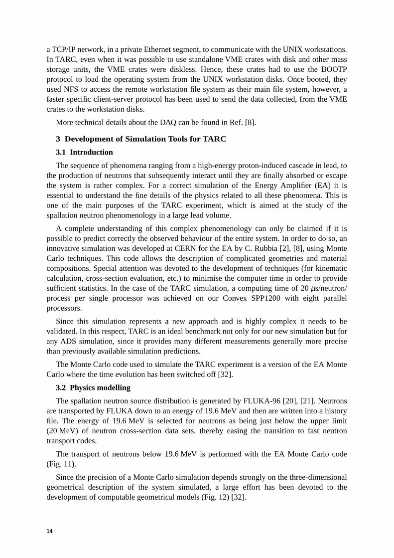
3 Development of Simulation Tools for TARC

3.1 Introduction

The sequence of phenomena ranging from a high-energy proton-induced cascade in lead, tothe production of neutrons that subsequently interact until they are finally absorbed or escapethe system is rather complex. For a correct simulation of the Energy Amplifier (EA) it isessential to understand the fine details of the physics related to all these phenomena. This isone of the main purposes of the TARC experiment, which is aimed at the study of thespallation neutron phenomenology in a large lead volume.

A complete understanding of this complex phenomenology can only be claimed if it ispossible to predict correctly the observed behaviour of the entire system. In order to do so, aninnovative simulation was developed at CERN for the EA by C. Rubbia [2], [8], using MonteCarlo techniques. This code allows the description of complicated geometries and materialcompositions. Special attention was devoted to the development of techniques (for kinematiccalculation, cross-section evaluation, etc.) to minimise the computer time in order to providesufficient statistics. In the case of the TARC simulation, a computing time of 20 µs/neutron/process per single processor was achieved on our Convex SPP1200 with eight parallelprocessors.

Since this simulation represents a new approach and is highly complex it needs to bevalidated. In this respect, TARC is an ideal benchmark not only for our new simulation but forany ADS simulation, since it provides many different measurements generally more precisethan previously available simulation predictions.

The Monte Carlo code used to simulate the TARC experiment is a version of the EA MonteCarlo where the time evolution has been switched off [32].

3.2 Physics modelling

The spallation neutron source distribution is generated by FLUKA-96 [20], [21]. Neutronsare transported by FLUKA down to an energy of 19.6 MeV and then are written into a historyfile. The energy of 19.6 MeV is selected for neutrons as being just below the upper limit(20 MeV) of neutron cross-section data sets, thereby easing the transition to fast neutrontransport codes.

The transport of neutrons below 19.6 MeV is performed with the EA Monte Carlo code(Fig. 11).

Since the precision of a Monte Carlo simulation depends strongly on the three-dimensionalgeometrical description of the system simulated, a large effort has been devoted to thedevelopment of computable geometrical models (Fig. 12) [32].

15

Fig. 11: Complete simulation of the interactions within the TARC lead volume of a single evaporationneutron produced by a 3.5 GeV/c primary proton and transported down to thermal energies.

Fig. 12: Picture of the simulated TARC geometry, showing the segmentation into local blocks,15 × 15 × 15 cm3, used in a second stage as local neutron generators for the various detector simulations(see Section 3.5).

3.3 Neutron cross-sections

Since a simulation is never better than the quality of the input data which are used, a specialeffort was made to provide the best possible neutron cross-section data. Our neutroncross-section data selection is taken from the latest compilations available [22]: ENDF/B-VI 4(USA), JENDL-3.2 (Japan), JEF-2.2 (Europe), EAF-4.2 (Europe), CENDL-2.1 (China),EFF-2.4 (Europe) and BROND-2 (Russia).

x

y

z

16

For each nuclide we have selected one evaluation out of those available on the basis of asystematic comparison [23]. In practice, the selection was done isotope by isotope according tothe evaluation of the resonances and the number of reaction cross-sections, as shown in Fig. 13for 137Cs for instance. When both the resonance region and the number of cross-sectionsevaluated are similar, then the most recently evaluated cross-section was selected. This resultedin a database of 800 nuclides with reaction cross-sections out of which 400 also have theelastic cross-section available. For all nuclides the corresponding information on isomericstates exists, and isomer-dependent reactions are treated correctly whenever they are available.

Fig. 13: Comparison of the 137Cs capture cross-section in the different databases available. The onechosen in this case for the EA Monte Carlo corresponds to the European Database (JEF-2.2).

All cross-section files have been processed and checked for inconsistencies with thestandard PREPRO-96 [24] code suite (LINEAR, RECENT, SIGMA1 and FIXUP) includingEAF-4.2.

All cross-section files produced by PREPRO-96 have been subsequently processed with aspecially written code package PROCESS [25] to create a direct-access library containingneutron cross-sections, cumulative secondary neutron energy distributions, and cumulativeneutron angular distributions (optionally).

3.4 Nuclear data

For nuclear transmutation studies, accurate mass and decay tables are needed. Here againwe have decided to go to the source of the data and we have created our own nuclear databasefrom the most up-to-date compilations available. The EET Nuclear Database selection [26] hasbeen assembled via a careful comparison of several sources. In particular, we have used theBrookhaven nuclear database [27], NUBASE [28], the National Radiological Protection Board(NRPB)database [29], the ICRP database [30] and nuclear data information from ENDF files.

For each isomer we store the atomic number, the chemical symbol, the mass number, theisomeric level, the isospin and parity, the mass excess, the half-life, the decay modes,branching ratios and decay-values where applicable, the natural isotopic abundance, and theinhalation and ingestion radiotoxicities [31].

10–4

10–3

10–2

10–1

1

10

102

1 10 102 103 104 105 106 107

Neutron energy (eV)

Cro

ss-s

ecti

on

(b

arn

)

ENDF/B-VI (USA)

JEF-2.2 (Europe)

JENDL-3.2 (Japan)

17

This database represents a major improvement over all existing ones for use in a MonteCarlo simulation. All available information about isomeric state decay and production has beenincluded. Nuclear data have been extensively checked for inconsistencies. In particular, alldecay paths are closed (i.e. terminate in a nuclide present in the database) and all branchingratios are consistent (i.e. sum = 100%).

The effort to have consistent databases was partly driven by practical considerations whichcome naturally if those databases are to be used in a simulation code. As a result, the fact ofhaving such an innovative code and such a reliable nuclear database makes our simulationprogram unique.

3.5 TARC general Monte Carlo code

In order to reduce the computing time needed to simulate the TARC experiment, it has beendecided to factorize the problem into a number of transport steps. In the first step the neutronsgenerated by the high-energy proton beam described by the FLUKA program are followed inthe lead block without detectors (‘Cube’ program) until they escape the block or are captured(Fig. 14).

Fig. 14: Complete simulation of the secondary neutron shower produced by a single 3.5 GeV/c primaryproton and transported in the entire TARC lead assembly until all the neutrons are captured or escape fromthe volume.

18

During this transport, a Data Summary Tape (DST) is produced. This is a condenseddescription of the neutrons escaping from the system or crossing internal boundaries4

providing source terms for further calculations. Creating such a tape has the advantage ofallowing repeated and various analyses with the same neutron source.

All crossings of the same neutron in and out of a block are recorded. In the successivetransport steps (‘Detector’ program), the effect of the surrounding lead can thus be neglectedand all incoming neutrons can be used as independent source neutrons and neutrons exiting theblock must be discarded. This simplifies the problem of the simulation of specific detectors.This approximation is correct only if the perturbation introduced by the detector is negligible.The magnitude of this perturbation can be evaluated by comparing the unperturbed and theperturbed exiting neutron spectrum which was done for each detector used in this study (seeSection 5).

While simulating a detector in a single instrumented block, the same neutron sample is runmore than once. This introduces some correlation in the events, but if the neutron sample islarge enough to be representative of the true neutron population, the error should be negligibleas the neutron histories will be different because of different random numbers.

The size of 15 cm around the instrumentation hole has been chosen to be large enough toallow the randomization of the neutron flux due to scattering in lead and to minimize theperturbations due to the presence of detectors.

All the neutrons escaping the lead assembly are recorded. These neutrons are used asindependent source neutrons in subsequent Monte Carlo calculations (‘CAVE’ program) wherethey are propagated into the area surrounding the lead assembly (hereafter called cave). Thosescattered back onto the lead assembly are recorded on a special history tape and used torecompute the detector response and evaluate the effect of background coming from neutronreflections on the concrete walls surrounding the experimental hall.

3.5.1 Systematic errors and technical checks on the Monte Carlo flux calculation

The TARC flux measurements have to be compared to the prediction of the TARC MonteCarlo chain: FLUKA for the spallation followed by Cube for neutron transport below19.6 MeV and finally by Detector, a specific code simulating the detector response. Thisdetailed comparison is an important prerequisite step for the understanding of AdiabaticResonance Crossing. It is therefore crucial to assess precisely the agreement between the dataand the prediction. This requires not only technical checks of the Monte Carlo calculation,ensuring that the whole chain, from FLUKA to the detector simulation is handled in aconsistent way, but also an evaluation of the systematic errors.

3.5.1.1 Systematics errors on the Monte Carlo simulation

The main systematic error contributions to the calculation of the neutron flux come from:

(1) The simulation of the spallation process in FLUKA and the neutron transport down to19.6 MeV for which the major sources of uncertainties can be summarized as follows:

– Cross-sections: (mostly reaction cross-sections) for protons and neutrons in theenergy range of interest (20 MeV to 3 GeV): The r.m.s. deviation between the

4. Each time the surface of one of the 240 15 × 15 × 15 cm3 boxes around the instrumented holes is crossedby a neutron, an entry is logged into the binary DST file.

19

cross-section adopted in FLUKA and available experimental data for lead is below10%. The error introduced in the calculations is significantly smaller in the bulk ofthe cascade since at the energies of TARC almost all protons interact inelasticallybefore being ranged out by ionization losses. Larger errors could arise at a fewinteraction lengths from the build-up region where, however, TARC results aremostly dominated by the diffusion of low-energy neutrons, rather than by localproduction due to the tails of the high-energy cascade.

– Neutron production model: The model used in FLUKA for the description ofnuclear interactions has been extensively benchmarked against several sets ofexperimental data. Double differential data about neutron production in lead areavailable for energies from 20 MeV to 3 GeV. The predicted double differentialspectra agree with the experimental data within a factor two and often much betterover the full range of energies and angles. The resulting agreement on angleintegrated spectra which are expected to be most relevant for TARC is typicallywithin 10–20% over most energy spectra. The total neutron multiplicity can bepredicted with errors not exceeding 10%. These errors are significantly reduced in athick target cascade owing to a significant averaging among different energies and tooverall constraints (like energy conservation).We can take 15–20% as an estimate of the systematic error coming from thesimulation of the spallation process.

(2) The simulation of neutron physics in lead below 19.6 MeV (mainly uncertainties inneutron cross-sections for lead). This contribution is estimated to be of the order of 10%.

(3) The knowledge of the chemical composition of the lead (the effect of the variousimpurities).

In this case, the TARC simulation was used to study the effect, on the neutron flux, of thevarious impurities contained in the lead. Four different lead qualities were considered: specialTARC lead of purity 99.99%, standard 99.99% lead purity, and purities of 99.985% and99.97%. Table 2 gives the detailed concentration actually used [33]. For the TARC lead, weused the measured concentrations, for the other lead qualities we changed the concentration forall the elements for which the vendor gives the concentration and for the others which are notknown we kept the same concentrations as for TARC.

We find that within a distance of 1.5 m from the centre of the lead assembly, the averagechange in fluence over the entire neutron energy range is smaller than 10% for qualities 99.99and 99.985. For quality 99.97 the decrease in flux below 5 eV reaches 30% (Fig. 15).

In order to assess the systematic error contribution from the uncertainty in the impuritycontent of the TARC lead, we have run the simulation with concentrations modified in thefollowing way: (1) all concentrations increased by two standard deviations (C = C + 2σc); (2)all concentrations decreased by two standard deviations (C = C – 2σc). Then we computed thefluence ratio between the two cases (Fig. 16). The change of fluence is generally small,negligible above 1 eV, and it reaches 6% at thermal neutron energy. This implies that the effecton the TARC neutron fluence measurement of the uncertainty in the impurity concentration inthe lead is negligible, over the energy range of interest.

20

Table 2: Details of the impurity contents for the various qualities of lead used in this study

Element TARC content (appm) 99.99% 99.985% 99.97%

Ag27Al75As

197Au11B

138Ba9Be

209Bi79Br

CCaCd

140Ce35Cl

59CoCr

133CsCu19FFe

69Ga74Ge

Hf202Hg

127IInIrK

139La7LiMg

55MnMo14N

23Na93Nb

142NdNi

16OOs

31P106Pd141Pr194Pt85Rb

Re

3.781.9E-25.5E-37.9E-42.7E-34.8E-44.9E-4

191.2E-2

1.21.6E-28.8E-21.1E-41.5E-23.6E-41.5E-25.5E-39.5E-22.3E-37.0E-33.0E-32.6E-36.8E-41.2E-13.1E-31.5E-38.6E-41.9E-21.6E-42.6E-43.2E-31.5E-32.4E-30.99

5.9E-34.1E-41.0E-33.3E-23.97

2.1E-37.2E-42.6E-31.5E-45.4E-36.8E-39.1E-4

1001

7.9E-42.7E-34.8E-44.9E-4

501.2E-2

1.20

8.8E-21.1E-41.5E-2

00

5.5E-310

2.3E-31

3.0E-32.6E-36.8E-41.2E-13.1E-31.5E-38.6E-41.9E-21.6E-42.6E-43.2E-31.5E-32.4E-30.99

5.9E-34.1E-41.0E-3

13.97

2.1E-37.2E-42.6E-31.5E-45.4E-36.8E-39.1E-4

1555

7.9E-42.7E-34.8E-44.9E-4

1101.2E-2

1.210

8.8E-21.1E-41.5E-2

55

5.5E-310

2.3E-315

3.0E-32.6E-36.8E-41.2E-13.1E-31.5E-38.6E-41.9E-21.6E-42.6E-4

55

2.4E-30.99

5.9E-34.1E-41.0E-3

53.97

2.1E-37.2E-42.6E-31.5E-45.4E-36.8E-39.1E-4

50510

7.9E-42.7E-34.8E-44.9E-4

2501.2E-2

1.210

8.8E-21.1E-41.5E-2

55

5.5E-310

2.3E-315

3.0E-32.6E-36.8E-41.2E-13.1E-31.5E-38.6E-41.9E-21.6E-42.6E-4

55

2.4E-30.99

5.9E-34.1E-41.0E-3

103.97

2.1E-37.2E-42.6E-31.5E-45.4E-36.8E-39.1E-4

21

Table 2: Details of the impurity contents for the various qualities of lead used in this study (Continuation)

Fig. 15: Variation of the ratio of neutron fluence in TARC lead to neutron fluence in lead with differentimpurity contents as a function of distance to the centre of the lead assembly. The neutron fluence isconsidered in the energy range from 1.0 eV to 5.0 eV.

Element TARC content (appm) 99.99% 99.985% 99.97%

103Rh102Ru

32SSb

45Sc80Se

SiSn

88Sr181Ta128Te232Th

Ti205Tl238U

VW

89YZnZr

9.5E-32.7E-34.0E-21.4E-11.5E-42.0E-21.3E-23.6E-31.3E-45.0E-22.2E-15.2E-43.5E-4

4.62.0E-41.8E-45.6E-37.2E-53.6E-34.1E-4

9.5E-32.7E-3

11

1.5E-42.0E-21.3E-2

11.3E-45.0E-2

55.2E-4

14.6

2.0E-41.8E-45.6E-37.2E-5

14.1E-4

9.5E-32.7E-3

1515

1.5E-410

1.3E-25

1.3E-45.0E-2

55.2E-4

1010

2.0E-41.8E-45.6E-37.2E-5

24.1E-4

9.5E-32.7E-3

55

1.5E-410

1.3E-210

1.3E-45.0E-2

55.2E-4

1010

2.0E-41.8E-45.6E-37.2E-5

104.1E-4

0.5

0.6

0.7

0.8

0.9

1

1.1

1.2

1.3

1.4

1.5

0 25 50 75 100 125 150 175 200

Distance from centre (cm)

Rat

io f

luen

ce (

new

co

nc)

/flu

ence

(re

al c

on

c)

At: 99.99

At: 99.985

At: 99.97

22

Fig. 16: Ratio of neutron fluences obtained with modified concentrations by ± 2 standard deviations withrespect to TARC nominal concentrations.

In order to study more specifically the effect of silver, we have run the simulation for asilver concentration increased by a factor 10 [C(Ag) = 37.8 ppm]. The ratio of fluences withthe increased silver concentration to the normal TARC concentration shows no effects down toneutron energies of 50 eV. A spectacular effect is found, as expected, below the main silverresonance of 5.2 eV, where the fluence drops by 20% (Fig. 17). This allows the effect of silverto be quantified. A variation of the silver concentration by 2 standard deviations, implies amaximum flux change by 0.7%, well below the other main sources of systematic errors.

We conclude that the error coming form the uncertainty in impurity concentrations in theTARC lead is safely negligible.

Fig. 17: Ratio of neutron fluences obtained with a modified silver concentration by a factor 10 with respectto the TARC nominal value.

0.6

0.7

0.8

0.9

1.0

1.1

1.2

1.3

1.4

–2 –1 0 1 2 3 4 5 6 7 8

Log10 [E(eV)]

Flu

ence

(+

2 si

gm

a) /

Flu

ence

(–

2 si

gm

a)

0.6

0.7

0.8

0.9

1.0

1.1

1.2

0 1 2 3 4 5 6 7 8

Log10 [neutron energy (eV)]

10×A

g le

ad /

stan

dar

d T

AR

C le

ad

23

The total systematic uncertainty in the flux calculation, over the neutron energy rangecovered by TARC, from thermal neutrons to a few MeV, even though hard to pin downprecisely, is estimated to be not larger than 25%.

3.5.1.2 Comparison between fluences from 2.5 GeV/c and 3.5 GeV/c protons as function ofthe neutron energy

It has always been assumed that the ratio of neutron fluences produced by protons ofdifferent energies is independent from neutron energy. We have verified, using our simulation,that this is indeed the case, at least in the neutron energy range between thermal and a fewMeV (Fig. 18).

Fig. 18: Ratio of fluences produced by 3.5 GeV/c and 2.5 GeV/c protons in TARC, as a function ofneutron energy (hole 10, z = +7.5 cm).

These systematic checks, together with many more trivial checks, allowed us to developconfidence in the results obtained, and gave us a good understanding of the detailed neutronbehaviour in lead, which is one of the main objectives of the TARC experiment.

3.5.2 TARC geometry description

The centre of the TARC reference system is at the geometrical centre of the lead volumeand the beam is along the positive z axis. The y axis is along the vertical direction. The generallayout of the assembly is shown in Fig. 19.

The 12 instrumentation holes and the beam hole have been included in the simulation.A virtual box of 15 × 15 cm2 in cross-section and 300 cm in length is placed around eachinstrumented hole (diameter 64 mm). This box is further subdivided into 20 slices along z,each one 15 cm long. The coordinates of the centres of the blocks in the TARC Monte Carloreference system are listed in Table 3.

Concerning the computer simulation of the back-scattered neutrons from the surroundingcase, a detailed description of the area surrounding the lead assembly is used [34] (see alsoSection 2).

A more complete description of the Monte Carlo technique developed both for the EnergyAmplifier and for the TARC experiment can be found in Ref. [8].

0.0

0.5

1.0

1.5

2.0

2.5

3.0

3.5

4.0

10–2 10–1 100 101 102 103 104 105 106 107 108

Neutron energy (eV)

Flue

nce

ratio

(pro

ton

3.5

GeV

/c) /

(pro

tons

2.5

GeV

/c)

24

Fig. 19: Schematic view of the simulated lead assembly. The z-axis is along the beam direction (into thepage).

Table 3: Summary of the coordinates of the centres of the 12 instrumented holes in the 334 ton leadassembly volume. The beam is introduced through a 77.2 mm diameter and 1.2 m long blind hole.

4 Study of the Energy–Time Correlation with CeF3 Counters

4.1 Introduction

In the TARC slowing-down lead spectrometer, a correlation develops between the time atwhich a neutron is observed and its velocity, hence its kinetic energy [35]–[38]:

(2)

where ξ, the average lethargy change, is given by:

. (3)

The diffusion mean free path λs of a neutron in the lead medium is practically constant overthe energy range between 0.1 eV and a few keV; v is the velocity of the observed neutron attime t, and v0 is the initial velocity corresponding to the energy E0 at which the neutron wascreated at time t = 0; mn and mPb are respectively the neutron and lead nucleus masses. This

Hole no. x (m) y (m) Hole no. x (m) y (m)

1357911

1.050.150.000.000.00–0.60

0.000.00–0.600.901.500.30

24681012

0.600.000.000.00–0.45–1.05

0.30–1.500.601.200.000.00

Y

X

8

67

2 11

1 3 10 12

5

4

9

t = −

2 1 1

0

λξ

sv v

ξ αα

α α≡ +−

( ) ≈ × ≡−( )+( )

−11

9 6 10 32

2ln . with Pb n

Pb n

m m

m m

25

relation can be rewritten in a slightly different form, relating the time of observation to themean energy of the neutron:

. (4)

It is relation (4) which is used by slowing-down spectrometers, in particular for severaldetectors in TARC (CeF3 counter, 3He scintillation counter and 6Li/233U counter), to obtain theenergy of neutrons from the measurement of the time between the arrival of the beam pulse,and the time of the neutron interaction in the detector.

The actual value of the K parameter has been experimentally determined (see Section 4.3).The quantity t0 can be considered as a time correction owing to the fact that the initial neutronis not created at infinite energy but at energy E0 and at velocity v0. In practice, all spallationneutrons are not created at the same energy, nor at the same place, nor at exactly the same timeand, in addition, the first part of the slowing down process is dominated by inelastic scattering.Therefore, t0 is a phenomenological constant which has to be estimated experimentally and, inour case, was checked using our simulation code and verified experimentally.

4.2 Analysis of the simulated correlation function

In practice, the energy–time relation is not a one-to-one relation but the mean value of acorrelation function C(E,t). The energy–time correlation function obtained by Monte Carlosimulation is presented in Fig. 20(a) and 20(b). These Monte Carlo data are displayed in adifferent way in Fig. 21, where one can observe that the quantity is almostconstant over the energy range 0.1 eV to 10 keV, with K = 173.3 keV × µs2 and t0 = 0.37 µs. Itis instructive to study more specifically the dispersion of K by showing several slices at fixedenergies of the distribution obtained (Fig. 22).

Fig. 20(a): Distribution of neutron energies and times from the Monte Carlo simulation.

E tK

t tK

mt

m

E( ) =

+( )= =

02

2

00

2 2where andn s

2sλ

ξλξ

t t E K+( ) =0

107

106

105

104

103

102

10

1

10–1

10–2

Neu

tro

n e

ner

gy

(eV

)

10–1 1 10 102 103 104

Time (µs)

26

Fig. 20(b): Evolution of the width of the correlation function shown in part (a), as a function of time (timedistribution for various neutron energy slices).

Fig. 21: Correlation function between energy E and the quantity as obtained from our MonteCarlo simulation.

Neu

tro

n e

ner

gy

(eV

)

Time (µs)10–1

10–2

10–1

1

10

102

103

104

105

106

107

10–2

10–1

1

10

102

103

104

105

106

107

10 101 102 103 104

4 5 6 7 8 9 10 20 30

(t+t0)×E1/2 (µs×keV1/2)

E (

eV)

10

102

1

103

104

105

106

107

10–1

10–2

t t E+( )0

27

Fig. 22: Energy slices of the correlation function displayed in Fig. 21, as a function of illustrating that K is indeed constant and showing the dispersion of the energy–time correlation. Gaussianfits are superimposed.

A cut at fixed t in the C(E,t) correlation function gives a quasi-Gaussian energy curve with atypical spread σE/E = 0.13 between 3 eV and 1 keV. A cut at fixed energy E also gives aquasi-Gaussian time distribution with a typical spread σt(E). Assuming that the shape at fixedenergy is given by:

(5)

the variation of σt(E) with E can be parametrized in the following way:

(6)

and

(7)

where E is in eV and σt in µs.

From the energy–time relation, in the low-energy region E < 4 eV, we can derive:

(8)

which is consistent with the theoretical calculation derived by Bergmann [37] which gives:

. (9)

200 300 400 500 600 700

(t + t0) √E

0

100

200

300

400

500

600

Co

un

ts

E = 100 eVGaussian fit

100

200

300

Co

un

ts

E = 1 eVGaussian fit

200 300 400 500 600 700

E = 1 keVGaussian fit

E = 5 eVGaussian fit

(t + t0) √E

t t E K+( ) =0

C E t tK

Ete

t t

,( ) ∝ ≡ −−

−( )2

220

σ t where

σ t for eV= + <25 231

1 74

. .E E

E

σ t ln for eV eV= + ×

< <30 541 0 306

8964 1600

..

E

EE

σ σE teVE t E

= = +( )

2 0 121 11 7

..

σEeVE E

= +( )

0 116 11 89

..

28

4.3 Experimental parameters of the correlation function

When measuring a neutron interaction between times t and t + ∆t its corresponding energyis located at within a quasi-Gaussian distribution. Using these properties we cancharacterize experimentally the energy–time correlation by measuring K and the timedispersion σt for well-defined neutron energies. Hence, for well-isolated strong and narrowknown neutron capture resonances, K and σt can be determined by detecting the timedistribution of neutron captures at these resonances.

For instance, a resonance at 5 eV with a width of 0.1 eV is located at t ≈ 200 µs with atime-width of 16 µs. The CeF3 detector described below (see Section 7) detects the prompt γ’sfollowing the neutron captures with a time resolution of typically 0.2 µs. An example of arecorded time spectrum is given in Fig. 23 for a tantalum target.

Fig. 23: Time spectra of neutron captures recorded with the CeF3 detector with and without a tantalumtarget. The lower spectrum corresponds to the captures in tantalum obtained after background subtraction.

In the case of tantalum, for the determination of K and σt we selected only the firstwell-isolated resonance at 4.28 eV (t ≈ 200 µs). After background subtraction, the selectedpeak is fitted with a Gaussian distribution superimposed onto a local exponential level:

. (10)

This type of fit gives, for the resonance studied, at energy Ei, both the associated time ti andthe dispersion σt (ti).

E t( )

0 200 400 600 800

Time (µs)

0

500

1000

1500

0 200 400 600 8000

500

1000

1500

2000

Cu

mu

late

d a

mp

litu

des

fo

r 10

9 p

roto

ns

Ta target

Background

Ta target - background

F t e et t t

t( ) = +− −

−( )( )α βτ σi

t i

2

22

29

The following targets natTa, natAu, natAg, natIn, natMn and 99Tc have been used. For thesetargets the selected resonances are given in Table 4 with the positions in the lead volume wherethe measurements were made.

Table 4: Experimental parameters for the determination of the energy–time correlation function, includingthe position at which the measurement was performed

The extracted energy–time correlation is shown in Fig. 24. Using relation (4) the Kcoefficient can be determined for each individual resonance. Figure 25 shows the variation ofthe extracted values obtained in different positions in the lead block as a function of theresonance energy. Throughout this study we fixed the t0 parameter at 0.37 µs, the value givenby a full Monte Carlo simulation. Note that for all resonances except that at 337 eV of 55Mnthe K determination is almost insensitive to t0, as expected since their ti values are largecompared to t0 (larger that 90 µs).

Fig. 24: Time vs energy for the selected resonances. Note that the error bars are smaller than the symbols.The straight line is the best log–log fit.

Target(resonance energy)

Time recorded(µs)

Width(µs)

Position[Hole, z (cm)]

K value(keV × µs2)

181Ta (4.28 eV)197Au (4.906 eV)109Ag (5.19 eV)99Tc (5.584 eV)115In (9.07 eV)107Ag (16.30 eV)55Mn (337 eV)

199.5 ± 1187.1 ± 1180.7 ± 1175.2 ± 0.9136.9 ± 0.7102.3 ± 0.622.4 ± 0.3

16 ± 2.717.5 ± 2.813.1 ± 2.114.7 ± 2.88.84 ± 1.16.0 ± 0.71.9 ± 0.4

10, 7.55, 82.5

12, 7.510, 7.55, 82.5

12, 7.55, 82.5

171 ± 1.8172.4 ± 1.8170.2 ± 1.8172.2 ± 1.8170.9 ± 1.9171.9 ± 2174.4 ± 5

1 10 100 1000Neutron energy (eV)

10

100

1000

Tim

e (µ

s)

Ta 4.28 eV

Au 4.906 eV

Ag 5.19 eV

Tc 5.584 eV

In 9.07 eV

Ag 16.30 eV

Tc 20.30 eV

Mn 337.00 eV

K = 172 keV.µs2

30

Fig. 25: Extracted experimental K-values for different energies at different positions in the lead volume.

From all K determinations, using the analysis of the various resonances mentioned above,the final experimental value of K is:

Kexp = 172 ± 2 keV × µs2

in agreement with the value extracted from fitting the corresponding simulation data:

Ksimulation = 173 ± 3 keV × µs2 .

Note that this experimental value of K is somewhat different from the estimation ofK = 165 keV × µs2 used by Chou and Werle [39] and we can only speculate that the differenceis due to their much smaller lead volume since they do not describe their energy–timecalibration nor the time distribution of their neutron source and the exact chemical purity oftheir lead.

We could not measure t0 with high precision, even with the 337 eV resonance of 55Mn. Thecorresponding t + t0 value is 22.6 µs and the time accuracy of the ti determination is estimatedto 0.2 µs. We checked that the value t0 = 0.37 µs corresponds to the central value of 55Mnmeasurements. The error on t0 is then set at ± 0.2 µs and is included in the time measurementerror.

Using the same well-separated neutron capture resonances in eight different targets it hasbeen possible to measure the σt dispersion at eight different neutron energies. After conversionof the time dispersion σt to energy dispersion σE, the relative energy dispersion σE/E wasplotted versus the neutron energy (Fig. 26). The comparison with the simulation results showsa good overall agreement, although experimental values of σE seem to be 15% higher than thesimulation data. This small discrepancy may be associated with flux perturbations due to thepresence of the detector material and target and is of negligible consequence for the use of theenergy–time relation for TARC.

1 10 100 1000

Neutron energy (eV)

160

165

170

175

180

185

K (

keV

.µs2 )

Ta 4.28 eVAu 4.906 eVAg 5.19 eVTc 5.584 eVIn 9.07 eVAg 16.30 eVTc 20.30 eVMn 337.00 eVK = 172 keV.µs2

± Uncertainty

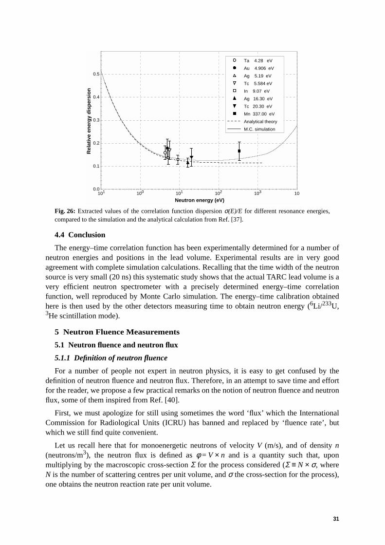
31

Fig. 26: Extracted values of the correlation function dispersion σ(E)/E for different resonance energies,compared to the simulation and the analytical calculation from Ref. [37].

4.4 Conclusion

The energy–time correlation function has been experimentally determined for a number ofneutron energies and positions in the lead volume. Experimental results are in very goodagreement with complete simulation calculations. Recalling that the time width of the neutronsource is very small (20 ns) this systematic study shows that the actual TARC lead volume is avery efficient neutron spectrometer with a precisely determined energy–time correlationfunction, well reproduced by Monte Carlo simulation. The energy–time calibration obtainedhere is then used by the other detectors measuring time to obtain neutron energy (6Li/233U,3He scintillation mode).

5 Neutron Fluence Measurements

5.1 Neutron fluence and neutron flux

5.1.1 Definition of neutron fluence

For a number of people not expert in neutron physics, it is easy to get confused by thedefinition of neutron fluence and neutron flux. Therefore, in an attempt to save time and effortfor the reader, we propose a few practical remarks on the notion of neutron fluence and neutronflux, some of them inspired from Ref. [40].

First, we must apologize for still using sometimes the word ‘flux’ which the InternationalCommission for Radiological Units (ICRU) has banned and replaced by ‘fluence rate’, butwhich we still find quite convenient.

Let us recall here that for monoenergetic neutrons of velocity V (m/s), and of density n(neutrons/m3), the neutron flux is defined as φ = V × n and is a quantity such that, uponmultiplying by the macroscopic cross-section Σ for the process considered (Σ ≡ N × σ, whereN is the number of scattering centres per unit volume, and σ the cross-section for the process),one obtains the neutron reaction rate per unit volume.

101 100 101 102 103 10

Neutron energy (eV)

0.0

0.1

0.2

0.3

0.4

0.5

Rel

ativ

e en

erg

y d

isp

ersi

on

Ta 4.28 eV

Au 4.906 eV

Ag 5.19 eV

Tc 5.584 eV

In 9.07 eV

Ag 16.30 eV

Tc 20.30 eV

Mn 337.00 eV

Analytical theory

M.C. simulation

32

This flux quantity must not be confused with the rate of particles crossing a surface element,which is a ‘current’ and which depends on the orientation of the surface with respect to thedirection of the particles.

We call ‘fluence’ the integral of the flux over a certain period of time, which is what wemeasure in TARC. We are interested in the neutron fluence produced by a proton of a givenenergy. In practice, we measure the ‘fluence’ per number of incident protons on the leadassembly. Most of our results are given as a fluence per 109 protons, in practice, integrating theflux over time from zero to infinity.

In TARC we used several different practical ways to compute the neutron fluence, in somecases as a cross-check that the procedures were correct:

(1) dN/dSperp is calculated as the number of neutrons crossing a small surface element dS,with dSperp = dS × cos θ, where θ is the angle between the neutron direction and thenormal to the surface element. One can note that in this process, considering all neutrondirections, if the small surface is a disk, then it will describe a spherical surface in spaceof area 4 × dS. The neutron flux φ will be the number of neutrons penetrating thisspherical surface per unit time from all sides (in an isotropic flux, one has φ/2 neutronspenetrating a 1 cm2 disk surface per second).

(2) It is more practical in Monte Carlo calculations to compute the average fluence in avolume element dV as d�/dV, where d� is the total track length of neutrons in the volumeelement dV. If the space distribution of neutrons does not change too abruptly, thisallows one, by selecting appropriate volume elements, to obtain better statistics. It isclear that the larger the region, the larger the systematic uncertainty on the flux. InTARC, we have tested several volumes (sphere with diameter equal to the diameter ofone hole, cylinder of length 15 cm with the same diameter as a hole, etc.) and found thatthe difference in flux obtained was negligible compared to usual statistical errors.

(3) In the data we usually record the number of interactions in a detector, therefore, wecompute the neutron fluence as the quantity (1/Σ) × dN/dV, where dN is the number ofinteractions in volume element dV.

Of course, the three methods are equivalent. In this TARC report, we usually quote thequantity F for fluence and φ for flux. Please note also that the isolethargic distributiondF/dln(E) is equal to E × dF/dE which in practice means that one is taking bins which have aconstant width in the natural logarithm of energy.

5.1.2 Properties of lead

Lead plays the major role in ARC, by providing neutrons by spallation, by having theappropriate properties already discussed in Section 1, in particular, its transparency to neutronsand its very uniform and high elastic scattering cross-section shown in Fig. 27, and its heavyatomic mass. It is these properties which determine the characteristics of the neutron fluence inTARC.

33

Fig. 27: Neutron capture and neutron elastic scattering cross-sections in natural lead (from the JENDL-3.2database).

5.2 Low-energy neutrons (En ≤ 50 keV) using energy–time correlation

5.2.1 6Li/233U target silicon detectors

The spallation neutrons, generated at time zero by GeV protons hitting the lead volume,give at position a neutron flux which is measured with a detection system usingthe exothermic reactions 6Li(n,t)α or 233U(n,fission). The reaction rate versus time isproportional to the quantity . Provided the cross-section σ(E) is known, themeasurement of the reaction rate gives an experimental access to the quantity asexplained in detail below.

5.2.1.1 The silicon detector and data recording

The charged particles produced in the reactions 6Li(n,t)α (Q = 4780 keV) or 233U(n,fission)(Q = 180 MeV) are recorded by two silicon detectors (Fig. 28) (with surface of 10 × 10 mm2

and thickness 300 µm). Two thin-foil targets of 1 × 1 cm2 separated by a 0.1 mm foil of lead,are inserted between two silicon detectors. The 6Li target is made of a lithium (95% of 6Li)fluoride (LiF) layer of either 50 µg/cm2 or 100 µg/cm2 deposited on a 50 µg/cm2 polyethylenebacking. The 233U target of 200 µg/cm2 is pure 233U electro-deposited on a 200 µm thickaluminium foil.

The output signal from the charge-preamplifier is encoded, after amplification, by an 8-bitflash-ADC (8192 channels, 0.1 µs/channel). Examples of flash records are shown on Fig. 29where alpha particles, tritons or fission fragments can be clearly identified. The beam intensityin this experiment ranges typically from 3 × 107 to a few 108 protons/shot.

A threshold on the amplitude spectra (Fig. 30) selects without ambiguity the chargedparticle signals: α’s, tritons or fission products. After processing of the data, time spectra ofdetected reactions by unit time ndet(t), normalized to 109 protons are obtained (Fig. 31).

10–4

10–3

10–2

10–1

1

10

102

10–5 10–3 10–1 10 103 105 107

Neutron energy (eV)

Cro

ss-s

ecti

on

(b

arn

)

Elastic

Capture

Natural lead

rr φ E t r, ,

r( )

φ σE t r E, , ( )r( )

φ E t r, ,r( )

34

Fig. 28: Schematics of the silicon-detector ensemble showing both the 233U and 6LiF targets.

Fig. 29: Examples of flash-ADC recordings for 6Li and 233U targets. In the 233U target flash, smallamplitude pulses correspond to α-particles emitted by 233U. The electronic gain used with the 233U targetis lower than for the 6LiF target. The counting of α’s from 233U was made with special runs with a highergain to separate better the α’s from the noise.

Stainless Steel Target Holder

Backing (CH2)n 50 µg/cm2

Silicon detectors(300 µm, 10 × 10 mm2)

12 m

m

37 mm

Preamplifiers

Vacuum

Stainless Steel Cylinder of ∅ 25 mm

6LiF Target

Lead Diaphragm of aperture 8 × 8 mm2

with a separator in the middle

LeadPrinted Circuit Boards

Aluminium Target HolderUranium (233U) Target

Pump

Channel (100 ns/channel)

0

100

200

3000 2000 4000 6000 8000

0 2000 4000 6000 8000

0

100

200

300

Am

plit

ud

e

triton

triton

alpha

triton

alpha

F.F.

F.F.

233U target

6LiF target

alpha

35

Fig. 30: Amplitude spectra for 6Li (upper histogram) and 233U (lower histogram) targets, showing theselection windows. The higher energy peak in the upper spectrum is produced by a pulser.

Fig. 31: Typical 6Li(n,t) and 233U(n,f) reactions time spectra recorded with the silicon detector andcomparison with the simulation (lines).

5.2.1.2 Extraction of neutron fluences from experimental measurements

The number of detected reactions detected in the time interval(t, t + ∆t), for a given number of incident protons (109), is given by:

, (11)

where Ntarget is the number of target atoms, is the mean neutron flux in the targetvolume at position , σ(E) is the 6Li(n,t) or 233U(n,f) reaction cross-section. Because of thetarget’s small thickness and the relatively small amount of detector material, with small

Amplitude

0

50

100

150

Co

un

ts

0

50

100

150233U targetwindow of selection

50 100 150 200 2500

200

400

600

Co

un

ts

0 200

50 100 150 200 2500 200

0

200

400

6006LiF targetwindow of selection

0 200 400 600 800

Time (µs)

10–1

100

101

102

Co

un

ts (

arb

itra

ry u

nit

)

6LiF Data233U Data

233U

6LiF

∆ ∆n n t r tdet det ,= ( )r

∆ ∆n t r N t E t r E Edet target d( , ) , , ( )r r= ( )∞

∫ε φ σ0

φ E t r, ,r( )

rr

36

neutron cross-sections, the local flux is not significantly perturbed by the target itself. This hasbeen checked explicitly by Monte Carlo simulation.

The expression (11) shows that for a time interval ∆t around t, the number of detectedreactions depend on the integral of over all neutron energies present at t in theinterval ∆t. We define, for a given t value, the flux as:

, (12)

where M(E,t) is a normalized probability distribution with which describesthe energy distribution of neutrons detected in the interval (t, t + ∆t). From relation (12) onededuces:

, (13)

appears to be the differential of the neutron fluence in the ∆t interval (integrated onE). The relation (11) can now be written as:

. (14)

We then define a mean cross-section :

. (15)

This mean cross-section at time t is assumed to be the mean cross-section at energy .This convolution is computed using the analytical parametrization of M(E,t) (see Section 4)and the JENDL database cross-section for (n,t) or (n,f) reactions. The fluence can beconverted into using the relation [Eq. (4), Section 4]. It corresponds to thefluence measured in the interval (t, t + ∆t). The differential neutron fluence at energy

is then given by:

. (16)

In order to determine absolute values of fluences, we still have to determine the quantityε Ntarget.

5.2.1.2.1 Experimental determination of ε Ntarget

This determination is made by using the 233U target–Si detector ensemble, in which the Sijunction is detecting both α’s coming from natural decay of 233U and fission fragment (ff) withrespective efficiency εα and εff. The number of α’s detected per second is given by:

, (17)

where λU3 is the radioactive 233U decay constant and NU3 the number of 233U atoms. Thenumber nα can be measured precisely, λU3 is well known.

The number of fission fragments detected per unit of time (shown in Fig. 31) is given by:

. (18)

The efficiencies εff and εα can be taken as equal to a common value ε because the 233Utarget is very thin (200 µg/cm2) and because collimators in front of the Si detector stop the α

φ σE t r E, ,r( ) ( )

φ E t r, ,r( )

φ E t r t F t r M E t, , , ,r r( ) = ( ) ( )∆ ∆

M E t E,( ) =∞∫ d0

1

∆ ∆F t r tE t r E E

M E t E E( , )

, ,

,

rr

=( ) ( )

( ) ( )

∞

∞∫∫

φ σ

σ0

0

d

d

∆F t r,r( )

∆ ∆n t r N F t r M E t E Edet target d( , ) ( , ) , ( )

r r= ( )∞∫ε σ0

σ

σ σ= ∞∫ M E t E E( , ) ( ) d0

E t( )

∆F t r( , )r

∆F E r( , )r

E t( )

f E r( , )r

E t( )

f E rF t r

E N

n t r t

E( , )

( , ) ( , )detrr r

= =∆∆

∆∆

1ε σtarget

nN

tNα

ααλ ε= =∆

∆ U3 U3

n t r t N E f E r Edet ff U3( , ) ( ) ( , )r r∆ ∆= ε σ

37

and fission fragments with large incident angles. The quantity ε × NU3 is extracted fromrelation (17). Using relation (18), is given by:

. (19)

The detection efficiency of the 6Li-target–Si junction ensemble was determined assumingthat the same neutron flux is measured both by 233U and 6Li detectors located in the sameposition. This normalization procedure introduces a systematic error estimated at 6%.

5.2.1.2.2 Errors on fluence determination with 6Li/233U silicon detector

The differential fluence is determined by time measurement using relation (19).This formula can be expressed as a function of time using the energy–time relation determinedwith the CeF3 measurements (Section 4). Assuming that for the main part of themeasurements, the cross-section (both for 6Li or 233U) is given by

,

where A is a constant, we get

,

neglecting t0. The term

and then becomes:

. (20)

In this relation ndet (t) represents the normalized number of captures per 109 protons. Thenndet (t) = 109 nmeasured (t)/I where I is the total number of protons in the run. Errors on t, K, andA are independent, then the uncertainty on f writes as:

. (21)

In this expression the first term δnmeasured/nmeasured represents the relative statistical errorand the others describe the relative systematic errors:

– the relative error on nα is estimated to be 6% mainly due to the normalization procedureused to calibrate the 6Li target measurement;

– the relative error on the beam intensity δI/I is 5%;

– the relative error on the coefficient A, δA/A, is estimated to be 10%;

– the error on time determination is δt = 0.5 µs (including the error on t0). Then δt/t rangesfrom 13% to 0.1% between 10 keV and 1 eV;

– The relative error δK/K has been estimated to be 1.2%.

Consequently, the experimental results for fluence determinations from thermal energies upto 10 keV have a relative systematic uncertainty of 14 to 28%.

f E r( , )r

f E r

n

n t r t

E( , )

( , )rr

= λσα

U3 det ∆∆

f E r( , )r

σ

σ ≈ A

E

σ ≈ At

K

∆∆

t

E

t

Kis

3

2

f E( )

f En t

n

t

A K( )

( )≈ λ

α

U3 det2

2

δ δ δ δ δ δ δα

α

f

f

n

n

I

I

n

n

A

A

t

t

K

K

=

+

+

+

+

+

2 2 2 2 2 2 2

22

measured

measured

38

5.2.1.3 Fluence energy and spatial dependence

A mapping was made in 72 positions scanning distances to the centre of the lead volumefrom 30 cm to 190 cm.

Typical fluence energy distributions from 3.5 GeV/c protons collected at several positions inthe lead volume are presented in Fig. 32. Figure 33 shows the spatial distribution of all fluxmeasurements for some selected neutron energy intervals (0.1 eV to 1 keV) as function of thedetector radial distance to the centre of the lead volume (negative values of r correspond toz < 0). These distributions are well fitted by Gaussian shaped curves.

The fluence shape is in agreement with the theoretical fluence for mono-energetic point-likeneutron source given by the Fermi age theory modified by an energy-dependentabsorption term:

; . (22)

Indicative values of the parameters, for 3.5 GeV/c protons, are:

E0 ≈ 1.5 MeV a ≈ (8 ± 1) 107 neutrons/cm2 per 109 protons

b ≈ 103 cm2 c ≈ 0.5 eV1/2

In fact the b parameter has to be adjusted to fit the data at different energies. Its variation hasbeen parametrized by a function bexp changing slowly with the neutron energy E. Thetheoretical value is given as a function of the lethargy and of the neutron mean free pathλs by:

with λs ≈ 2.76 cm . (23)

The experimental value has been found slowly energy-dependent with theparametrization:

. (24)

A comparison of this model with experimental results is shown in Fig. 34.

Note that this representation provides a simplified and compact way to describe all theexperimental data assuming that fluences have a quasispherical symmetry, although this is notstrictly exact for short radial distances near the spallation source centre or large radial distancesnear the edge of the lead volume. In principle the parameter a can lead to the number ofneutrons created per proton by the spallation process. But the a value is extracted by fitting theflux for neutron energies below 1 keV and at this stage there has been sizeable absorption,leakage out of the lead assembly, and (n,xn) production.

While most of the measurements have been made using a proton beam of 3.5 GeV/c, a fewmeasurements have also been made at 2.5 GeV/c. The associated fluence energy spectra forboth beam energies are compared. As expected these fluences are proportional to each other, inthe measured energy range. This is illustrated in Fig. 35 and leads to the measured ratio:

. (25)

f E r0( , )r

f E ra

E u

r

bu

c

E0 3 2

2

( , ) exp exp/r = −

−

u

E

E= ln 0

bth( )

bth

s= 43

2λξ

bexp( )b

bEexp

th= +( )0 922 0 0181. . ln

RE

Ec

c= = ± ( )

ΦΦ

3 5

2 51 44 0 05.

.

( )

( ). .GeV/

GeV/stat.

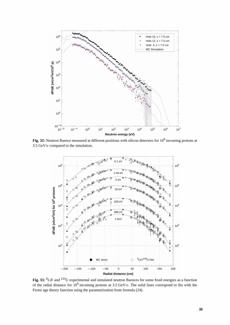
39

Fig. 32: Neutron fluence measured at different positions with silicon detectors for 109 incoming protons at3.5 GeV/c compared to the simulation.

Fig. 33: 6LiF and 233U experimental and simulated neutron fluences for some fixed energies as a functionof the radial distance for 109 incoming protons at 3.5 GeV/c. The solid lines correspond to fits with theFermi age theory function using the parametrization from formula (24).

10—2 10—1 100 101 102 103 104 105 106 107

Neutron energy (eV)

10—1

100

101

102

103

104

105

106

dF

/dE

(n

/cm

2 /eV

/109

p)

Hole 10, z = 7.5 cm

Hole 12, z = 7.5 cm

Hole 4, z = 7.5 cm

MC Simulation

—200 —150 —100 —50 0 50 100 150 200

Radial distance (cm)

1 keV

MC simul. 6LiF/233U Det.

480 eV

100 eV

18 eV

5 eV

1.46 eV

0.1 eV

dF

/dE

(n

/cm

2 /eV

) fo

r 10

9 p

roto

ns

106

105

104

103

102

106

105

104

103

102

40

Fig. 34: Isolethargic fluence experimental spectrum EdF/dE compared with the Fermi age theory, with andwithout the absorption term.

Fig. 35: Example of ratio of differential fluences obtained with the two beam momenta (3.5 GeV/c and2.5 GeV/c) both measured at the same position (hole 10, z = +7.5 cm) inside the lead volume.

This result is not too far off the expected value coming from the ratio of beam kineticenergies Rkinetic = 1.59 5, if the number of primary spallation neutrons is proportional to theproton kinetic energy.

5. We have data for proton momenta of 3.568 GeV/c and 2.499 GeV/c. The kinetic energy is thenT = 2.75 GeV and T = 1.73 GeV, respectively.

10–2 10–1 100 101 102 103 104 105

Neutron energy (eV)

105

106

107

108

E d

F/d

E (

n/c

m2 /

109

pro

ton

s)

Data (hole 10, z =7.5 cm, r = 46 cm)

Fermi age theory with absorption

Fermi age theory

10–1 100 101 102 103 104

Neutron energy (eV)

0.0

0.5

1.0

1.5

2.0

2.5

3.0

3.5

4.0

Rat

io

flux (2.75 GeV) / flux (1.73 GeV)

mean ratio

41

5.2.1.3.1 Comparison with our simulation

The measured fluence at various positions was compared to Monte Carlo simulations(Fig. 36). In order to show a global comparison of simulation and data, we calculated the ratior = ⟨data/MC⟩ . The bracket means that the averaged value is made over the energy range 1 eVto 1 keV. The distribution of the residuals, 1 – r, obtained for all runs (Fig. 37), shows excellentaverage agreement with the simulation with a narrow dispersion of the r values (8% consistentwith the run-to-run fluctuations).

Fig. 36: Isolethargic fluence E × dF/dE at 3.5 GeV/c at different positions compared with Monte Carlosimulation.

Fig. 37: Number of runs versus 1 – r (see text). 1 – ⟨r⟩ = 0.05 ± 0.09. A Gaussian fit is also shown. Themean value of the distribution is found to be 0.05 ± 0.09.

10–2 10–1 100 101 102 103 104 105 106 107

Neutron energy (eV)

104

105

106

107

E×d

F/d

E (

n/c

m2 /

109

p)

Hole 10, z = 7.5 cm

Hole 12, z = 7.5 cm

Hole 4, z = 7.5 cm

MC Simulation cm

—0.5 —0.3 —0.1 0.1 0.3 0.5

1 — r

0.0

2.0

4.0

6.0

Nu

mb

er o

f ru

ns

42

5.2.2 3He scintillation counter

5.2.2.1 Description of the counter

The 3He scintillation detector uses the 3He(n,p)3H reaction which has a positive Q value of0.764 MeV [41].

The energy lost by the charged products of the reaction slowing down in the gas mixtureleads to the emission of light with an intensity proportional to the energy deposited in the gas.The photons emitted in the atomic de-excitation and recombination processes, following theelectromagnetic interactions with the electrons of the gas atoms through which the reactionproducts lose their kinetic energy, have an energy of about 20 eV (62 nm) [42]. In order toincrease the scintillation light output, instead of using pure 3He we used a mixture of 3He withXe since the number of scintillation photons per MeV for Xe is three times more than for Heand since a mixture of at least 10% Xe (the rest is He) gives as much light output as pure Xe[42]. Xenon produces light at 172 nm and is also used as a wavelength shifter that shifts part ofthe 3He scintillation photons from 62 nm to 172 nm [42].

In order to increase further the light output and match it to the maximum response of thephotomultiplier photocathode used to observe the gas scintillation (above 300 nm), a layer ofp-terphenyl [41] was vacuum-deposited on a highly reflective coating of MgO [43] on the innerwalls and on the base of the chamber. P-terphenyl is a wavelength shifter that absorbs theultraviolet emissions at 172 nm and part of the 20 eV photons, re-emitting at 340 nm [44].P-terphenyl is also evaporated on the internal surface of the quartz window of the chamber(cut-off at 160 nm [45]) to wavelength-shift the direct photons.

The 3He scintillation chamber (Fig. 38) is cylindrical with internal diameter 40 mm andlength 59 mm and is made of stainless steel. For the optical connection to the photomultiplierwe used a quartz window 4 mm thick, sitting on a copper ring with 27 mm internal diameterand 4 mm width.

Fig. 38: Schematics of the 3He scintillation chamber.

We note that p-terphenyl evaporates at room temperature and becomes an impurity in thegas, thus quenching the photon emission [42]. In order to calibrate continuously the variationof the efficiency of the gas mixture with time, we installed a 5.5 MeV 241Am alpha source at

PM

241Am(5.5 MeV alphas)

p-Terphenyl

70% 3He - 4He + 30% Xe

MgO

Quartz (4 mm)

MgO+ p-Terphenylon a copper ring

active surfaceof the source

59 m

m

40 mm

INOX

15 mm6 mm

43

the bottom of the chamber (in the centre). The gas deterioration, due to the evaporation of thep-terphenyl, is observed as the displacement of the alpha photopeak with time (Fig. 39). Thediameter of the active surface of the source is 6 mm while the diameter of the whole surface is15 mm. In order to minimize shadowing effects from the source we installed around the activesurface of the source a copper ring on which MgO and p-terphenyl layers were deposited.

The range of 1.5 cm for 5.5 MeV α particles [46] and the corresponding mixture werechosen because both the total pressure (3.93 bar) of the mixture and the consumption of 3Heare low, while the light output is satisfactory, according to the results of the measurementsshown in Fig. 40.

Fig. 39: Monitoring the 3He counter efficiency with the 241Am 5.5 MeV alpha photopeak for the samefilling of the chamber. Curves 1, 2, 3 and 4 correspond to times t = 0, 1 h, 2 h and 4 h respectively.

Fig. 40: Mean position of the 5.5 MeV alpha photopeak as a function of Xe percentage for a 4He–Xemixture. The lines are guides for the eye (made with a polyonymial fit), while the error bars represent thesigmas of the distribution of every photopeak (as calculated with Gaussian fits).

12

3

4

ADC channel number

Co

un

ts p

er c

han

nel

0

100

200

300

400

500

600

200 400 600 800 1000 1200 1400

Range 1 cm

Range 1.5 cm

Range 2 cm

Mea

n p

eak

po

siti

on

(A

DC

ch

ann

el)

Xe fraction (%)0 5 20 25 30 35 401510

1200

1000

800

600

400

200

0

44

5.2.2.2 Measurements and data analysis

There are two sets of measurements: data taken in October 1996 at the proton momentum of3.5 GeV/c and in May 1997 at the proton momentum of 2.5 GeV/c. Table 5 shows all thepositions studied during the two sets of measurements.

Table 5: Summary of positions (hole number and z-coordinate) at which measurements were made inTARC with the 3He scintillation counter. For the definition of holes and coordinates see Section 2. The unitis centimetres.

To obtain the time spectrum for the above positions, the signal of the photomultiplier (PM)is directed to a 200 MHz channel PM amplifier and then to an 8-bit ICARUS FADC with asampling rate of 100 ns.

For each of the above positions we also took measurements using the mixture (1.18 bar Xe,2.75 bar 4He) for background subtraction. These background measurements have beennormalized to the same proton beam intensity and subsequently subtracted from the spectra.

In order to evaluate the deterioration of the gas mixture with time (due to evaporation ofp-terphenyl), we made at the beginning of every run one calibration measurement using theinternal α source in the chamber. Then by fitting the α photo-peak to a Gaussian we extractedthe number of photoelectrons (the number of photoelectrons is equal to the square of the ratiomean over sigma of the Gaussian), corresponding to the α photopeak for every calibrationmeasurement. In this way, for each run we could obtain the gas calibration factor.

For each run of the first set of measurements in 1996 (3.5 GeV/c) we accepted the eventswith a PS shot intensity between 3 × 107 and 9 × 107 protons while for the second set ofmeasurements in 1997 (2.5 GeV/c) we accepted the events with shot intensity between 107 and5 × 107 protons. We note here that for the second set of measurements (2.5 GeV/c) the beamintensity was a factor of two smaller. We normalized every shot to a beam average of6 × 107 protons per shot (for both sets) and we also corrected for the gas deterioration using thecalibration measurements. For every run we added all the pulses bin by bin, divided by thenumber of shots and thus calculated the mean pulse (Fig. 41). The same procedure was appliedin order to obtain the mean pulse for every background run (Fig. 41). The backgroundsubtraction was made using the calculation of the mean pulses of the signal (3He) and of thebackground (4He) runs for all corresponding runs (Fig. 42).

The ratios of data taken with 3.5 GeV/c protons over data taken with 2.5 GeV/c protonspresented in Table 6 are expected to follow the ratio of the kinetic energies of the beams whichis 1.59. The fit of the ratio of data for hole 3, at z = +67.5 cm for the two different protonmomenta (Fig. 43) shows that indeed this ratio is constant over the neutron energy rangeconsidered and consistent with the expected value.

3.5 GeV/c 3.5 GeV/c 3.5 GeV/c 2.5 GeV/c 2.5 GeV/c 2.5 GeV/c 2.5 GeV/c

Hole 3 Hole 10 Hole 1 Hole 3 Hole 10 Hole 1 Hole 8

+7.5+37.5+67.5+97.5+112.5

+7.5

+67.5

+7.5

+67.5

+112.5

+7.5

+67.5

+112.5

+7.5

+67.5

+7.5

+67.5

+112.5

+7.5

45

Fig. 41: Mean signal i.e. integrated charge (FADC channel) (3He) [upper curve] and mean background(4He) [lower curve] pulses with 100 ns binning at hole 10, z = +7.5 cm, 500 V (2.5 GeV/c proton run).

Fig. 42: 3He signal i.e. integrated charge (FADC channel) minus background (4He) with 100 ns binning athole 10, z = +7.5 cm, 500 V (2.5 GeV/c proton run).

Time (0.1 s)

FA

DC

ch

ann

el

500

400

300

200

100

01000 2000 3000 4000 5000 6000 7000 80000

Time ( s)

Sig

nal

(F

AD

C c

han

nel

)

10

102

100 200 300 400 500 600 7000

46

Fig. 43: Example of ratio of fluence with 3.5 GeV/c protons over fluence with 2.5 GeV/c protons forhole 10, z = +7.5 cm. The fitted ratio 1.67 is consistent with the value 1.59 ratio of the kinetic energies ofthe proton beam.

Table 6: Ratio of 3He signal i.e. integrated charge (FADC channel) minus background (4He) for 3.5 GeV/cproton runs over the signal for 2.5 GeV/c proton runs as calculated by fitting the ratios of thecorresponding data for various holes and positions. (The errors shown are statistical while the systematicerror is 6%.)

5.2.2.3 Comparison of data with Monte Carlo simulation

We used the TARC Monte Carlo simulation code developed by the CERN EET group [32]in order to make a comparison with the measurements. The complete geometry of the 3Hescintillation chamber has been described in the simulation. The device was placed in themiddle of a DST volume (15 × 15 × 15 cm3 lead box with a hollow cylinder of radius 3.2 cmand length 11 cm that contains air).

Average ratios from 3He measured signals i.e. integrated charge (FADC channel) correctedfor background (4He) to Monte Carlo simulation for the different positions and holes and forthe three different sets of measurements corresponding to PM voltages of 450, 500 and 550 V(Table 7) show that the data are consistent with the simulation of the entire set of operatingparameters. An example of ratio distribution is shown in Fig. 44.

Hole z position (cm) Ratio

3333101011

+7.5+37.5+67.5+112.5+7.5+67.5+7.5+67.5

1.422 ± 0.0051.482 ± 0.0051.618 ± 0.0041.528 ± 0.0061.676 ± 0.0051.719 ± 0.005 1.636 ± 0.0061.456 ± 0.006

Time (µs)

Rat

io:

dat

a at

3.5

GeV

/c /

dat

a at

2.5

GeV

/c

100 200 300 400 500 600 70000

0.25

0.50

0.75

1

1.25

1.5

1.75

2

47

Table 7: Ratios of 3He signal i.e. integrated charge (FADC channel) background (4He) subtracted toMonte Carlo for various positions and PM voltages for 3.5 GeV/c protons

Fig. 44: Fits of the ratios of 3He signal i.e. integrated charge (FADC channel) background (4He) subtractedto Monte Carlo for various positions in hole 3, a PM voltage of 500 V and for 3.5 GeV/c protons.

We also made tests of the 3He scintillation chamber using neutrons produced by thet(p,n)3He reaction at the Bordeaux van de Graaff accelerator. The aim of these measurements(Fig. 45) was to determine the ratio of the light emission from the 3He(n,p)3H reaction withthermal neutrons to the light emission of the 5.5 MeV 241Am alpha source.

The ratio of the thermal neutron peak over the alpha peak was found from thesemeasurements to be 0.137 ± 0.002, which is compatible with the expected value of the ratio0.764 MeV/5.5 MeV = 0.139.

Hole z position (cm) 450 V 500 V 550 V

3333101011

+7.5+37.5+67.5+112.5+7.5+67.5+7.5+67.5

1.013 ± 0.0221.017 ± 0.0170.875 ± 0.0120.967 ± 0.0121.077 ± 0.0161.079 ± 0.0140.964 ± 0.0110.964 ± 0.010

0.990 ± 0.0210.981 ± 0.0160.928 ± 0.0130.951 ± 0.0111.112 ± 0.0161.006 ± 0.0121.012 ± 0.0100.981 ± 0.009

0.977 ± 0.0241.026 ± 0.0200.940 ± 0.0130.958 ± 0.0101.098 ± 0.0190.974 ± 0.0121.000 ± 0.0950.953 ± 0.085

Hole 3, z = + 7.5 cm Hole 3, z = + 37.5 cm

Hole 3, z = + 67.5 cm Hole 3, z = + 112.5 cm

Time (µs) Time (µs)200 400 6000 200 400 6000

Time (µs) Time (µs)200 400 6000 200 400 6000

0

0.2

0.4

0.6

0.8

1

1.2

1.4

1.6

1.8

2

0

0.2

0.4

0.6

0.8

1

1.2

1.4

1.6

1.8

2

0

0.2

0.4

0.6

0.8

1

1.2

1.4

1.6

1.8

2

0

0.2

0.4

0.6

0.8

1

1.2

1.4

1.6

1.8

2χ2 / ndf : 79.13 / 72AO .9896 ± .2114E-01

χ2 / ndf : 85.47 / 72AO .9812 ± .1647E-01

χ2 / ndf : 146.4 / 72AO .9508 ± .1052E-01

χ2 / ndf : 104.3 / 72AO .9282 ± .1253E-01

48

Fig. 45: (a) Signal and background measurements in logarithmic scale for thermal neutrons; (b) Signalafter background subtraction in linear scale (without subtracting the alpha peak).

5.2.2.4 Neutron fluence calculation

The neutron fluence was calculated using the relation:

(26)

where Nevents(E) is the number of events as a function of energy in the counter volume, σ(E)the cross-section for the 3He(n,p)3H reaction, F(E) the neutron fluence, and Natoms the numberof 3He atoms in the counter volume equal to 11.017 × 1020 atoms for the gas mixture we used.The number of events as a function of time is obtained by converting the data spectrum via thecalibration factor of the FADC for a given photomultiplier voltage. The data spectrum is theresult of the subtraction of the mean background spectrum [the one obtained using only 4Hei.e. integrated charge (FADC channel) as a function of time] from the mean signal spectrum(the one obtained using the mixture of 3He and 4He).

In order to obtain the number of events as a function of energy we use the meanenergy–time relation:

. (27)

For a given binning in energy (100 equal lethargy bins from 10–2 eV up to 105 eV), for eachenergy bin the corresponding time window is calculated via the mean energy–time relation.The contents of the time bins within this time window are taken from the data spectrum(100 ns binning) and are subsequently converted, via the FADC calibration factor for a givenphotomultiplier voltage, to number of events.

Selected from all the positions measured in the lead assembly (Table 5), Fig. 46 presentstypical fluence measurements as a function of neutron energy for hole 3, as obtained from thedata for a photomultiplier voltage of 450 V with a binning of 100 ns at a proton momentum of3.5 GeV/c.

a)

b)

3He and Xe

4He and Xe

5.5 MeV alpha peak

Thermal neutron peak

5.5 MeV alpha peak

ADC channel number

ADC channel number

Co

un

ts p

er c

han

nel

Co

un

ts p

er c

han

nel

200 400 600 800 1000 12000

200 400 600 800 1000 12000

0

100

200

300

400

500

600

1

10

102

103

N E E F E Nevents atoms( ) = ( ) × ( ) ×σ

Et

eVs

[ ] =[ ] +( )

172000

0 372µ .

49

Fig. 46: Neutron fluences (E × dF/dE) versus neutron energy, for 109 protons of 3.5 GeV/c in hole 3. Thecurves correspond, from top to bottom, to the positions: z = +7.5 cm, +37.5 cm, +67.5 cm, +97.5 cm, and+112.5 cm.

5.2.2.5 Systematic errors

We estimate that the systematic errors are:

– 5% in the proton intensity, mainly related to the Al(p,3pn)24Na cross-section uncertainty,used for the beam transformer calibration.

– 3% due to the uncertainty in the absolute gas pressure. The precision of the absolutepressure meter is 0.001 bar. However, the uncertainty of 10° due to the cooling trapinduces an error of approximately 3%.

– 0.6% due to error on the estimation of K in the energy–time relation from ∆k/k = 1.2%.

– 12% due to the conversion of the FADC channels to number of events. The factorscontributing to this uncertainty are 2.5% from the range of the FADC (256 channelscorrespond to 3.00 ± 0.075 mV); 7% from the amplification precision of Lecroy 612 Awith an amplification factor 10 ± 0.07; 5% from the precision of the 11-bit Lecroy ADC[47], 512 ± 25.6 pC, and 12% in the gain due to the error in the value of the coefficient αset by the dynode material and to the geometry of the photomultiplier. (The error in thegain depends on the voltage and is 12% for 450 V, 10% for 500 V, 8.4% for 550 V and6.7% for 600 V.)

– Error on the value of t and t0, dominant at high energy region (8% at 1 keV, 54% at50 keV).

From the above contributions the error in the proton intensity is common for all detectors inthe TARC experiment, while the errors on the energy–time relation and on the value of t and t0are common for the 3He scintillation detector and the 6LiF detectors. In summary thesystematic error ranges from 13.5% to 55% for neutron energy from 0.1 eV to 50 keV.

Flue

nce

(E ×

dF/

dE) (

neut

rons

/ cm

2 fo

r 10

9 pr

oton

s of

3.5

GeV

/c)

10–1 100 101 102 103 104 105

Neutron energy (eV)

107

106

105

50

5.2.2.6 Consistency with other flux measurements in the TARC experiment

In this section we present a comparison with the data taken with the lithium fluoride (6LiF)detectors (Figs. 47 and 48), (see Section 5.2.1). These detectors have a neutron energy rangesimilar to that of the 3He scintillation detector.

Fig. 47: Neutron fluence per electronvolt for 109 protons at 2.5 GeV/c as a function of distance from thecentre of the lead volume at energies 0.1 eV, 1 eV, 5 eV, 10 eV, 18 eV, 100 eV, 480 eV, 1 keV, 10 keV and50 keV from the 3He scintillation detector, 6LiF silicon detectors and Monte Carlo. Lines representGaussian fits to the Monte Carlo points.

Fig. 48: Neutron fluence per electronvolt for 109 protons at 3.5 GeV/c as a function of radial distance fromthe centre of the lead volume at energies 1.46 eV, 4.96 eV, 18.9 eV, 100 eV, 480 eV, 10 keV and 50 keVfrom activation foils, the 3He scintillation detector and Monte Carlo for two cases: with and without thepresence of the 3He detector. Lines represent Gaussian fits to the Monte Carlo points (diamond shape)without detector.

dF

/dE

(n

/cm

2 /eV

per

109

pro

ton

s)

Distance to the centre (cm)0 20 40 60 80 100 120 140 160 180 200

50 keV

10 keV

1 keV

480 eV

100 eV

18 eV10 eV5 eV

1 eV

Monte Carlo3He Scintillation6LiF Detector

0.1 eV

106

105

104

103

102

10

1

106

105

104

103

102

10

1

dF

/dE

(n

/cm

2 /eV

per

109

pro

ton

s)

Distance to the centre (cm)

106

105

104

103

102

10

1

106

105

104

103

102

10

10 20 40 60 80 100 120 140 160 180 200

1.46 eV (ln)

4.96 eV (Au)

18.9 eV (W)

100 eV

480 eV

10 keV

50 keV

Monte Carlo3He Scintillation

Activation Foils

Monte Carlowith 3He detector

51

The energies 1.46 eV, 4.96 eV, and 18.9 eV have been chosen because at these energies thegold, indium, and tungsten used in activation foils exhibit strong resonances in their neutronabsorption cross-sections (see Section 5.2.3). The energy of 480 eV is of particular interest,since it is the energy of the 98Mo capture resonance.

As seen from all the above plots, the data from different detectors are consistent betweenthemselves and are also consistent with the Monte Carlo predictions.

5.2.3 Triple-foil activation

Some additional checks were made of the neutron fluence at low energies, using theactivation foil technique [48]. The method consists of activating in the TARC lead volumetriple foils of a material such as typically gold (197Au), with a very high resonance in itsneutron capture cross-section (27 405 barns at 4.9 eV in the case of gold). The foil thickness ischosen so that the outer foils are essentially opaque to neutrons at the resonance energy. Thedifference between the average activity of the outer foils and the activity of the central foil,provides a measurement of the neutron fluence at the resonance energy. As an example, in thecase of gold, we find that both the average activity of the outer foils and the difference betweenouter and central foils are well reproduced by our Monte Carlo simulation (Fig. 49). Thisimplies that the neutron fluence at 4.9 eV is correct. Similarly the neutron fluence at 1.46 eVand 18.9 eV was checked with 115In and 188W foils respectively.

A summary of neutron fluence measurements from all the low energy detectors (6Li/233U,3He scintillation mode and activation foils) (Fig. 48) shows that all the measurements areconsistent with one another and with the Monte Carlo prediction. We estimate that in the caseof activation foils the systematic error on the fluence measurement is about 10%.

Fig. 49: Experimental and Monte Carlo mean activity S and resonance activity A for gold foils.

5.2.4 Thermoluminescence detectors

A further test was made using the thermoluminescence technique to probe the neutronfluence below 0.5 eV [49]. The technique is well known for measuring radiation doses. In ourcase we irradiated pairs of 6LiF–7LiF sandwiches, either covered with cadmium to shield fromthe neutrons below 0.5 eV or uncovered. From the measurements of the neutron dose (from the

Distance from centre (cm)

Act

ivit

y fo

r 10

9 p

roto

ns

(Bq

)

00

0.1

0.15

0.05

0.2

0.25

0.3

0.35

0.4

0.45

20 40 60 80 100 120 140 160

Exp S

Exp A

MC S

MC A

52

difference between 6Li and 7Li), and taking advantage of the fact that the LiF material wasthick enough to totally absorb neutrons below 0.5 eV, the integral neutron fluence through thedetector could be evaluated (Fig. 50), and was found consistent with the simulation. Thiscompletes our low energy checks of the neutron fluence in TARC.

Fig. 50: Thermal neutron fluence (E < 0.5 eV) as a function of the radial distance in the lead block. Theline is an eye guide connecting the experimental points (triangles). The black squares are Monte Carlosimulation.

5.3 High-energy neutrons (10 keV to 2 MeV) with 3He ionization counters

5.3.1 Introduction

As already explained in previous sections, it is neutrons in the low-energy range that aremost important for long-lived fission fragment transmutation. Neutron energies up to 10 keVare covered by several detectors, mainly the 3He scintillation counter and the (6LiF, 233U) Sidetectors. However, the birth of neutrons takes place in the high-energy range, where thecompetition between capture resonances, elastic and inelastic collisions, and multiplicative(n,xn) reactions will determine the available neutron flux at lower energies. In addition, theknowledge of the neutron flux in the region of the spallation cascade, dominated by thehigh-energy neutrons, is very important for the design of the spallation target, one major itemof any ADS design, in particular for the Energy Amplifier. The 3He ionization chamber is themain TARC detector covering the neutron spallation energy region.

Ionization chambers filled with 3He are standard detectors for fast neutron spectroscopy i.e.in the energy range from tens of keV to a few MeV [50]. Neutrons entering such detectorsinteract with the 3He gas through the exothermic reaction:

n + 3He → p + 3H + Q where Q = 764 keV.

The simplicity of the well-known cross-section together with the noble gas properties andthe high Q-value make 3He detectors well-suited for spectrometry both in the proportional or

Radial distance (cm)

Neu

tro

n f

luen

ce w

ith

E <

0.5

eV

(n

/cm

2 /10

9 p

roto

ns)

–200 –150 –100 –50 0 50 100 150 200

105

106

53

ionization modes. In the latter case, in most of the applications, a Frisch grid (Figs. 51 and 52)has been added in order to maximize the energy resolution. Resolution is the most crucialparameter when one is trying to have the lower end of the detectable neutron energy spectrumseparated from the overwhelming thermal peak background given by the (n,p) reaction. Themost important factors that affect the energy resolution are general parameters such asamplifier noise, pulse shaping, mechanical vibrations, homogeneity of the electric field, andpeculiar ones linked to neutron detection such as wall effects and recoil effects at highenergies.

5.3.2 Description of the counter

Since the best results have been obtained with gridded ionization chambers of theCutler–Shalev type [51], our 3He spectrometer is based on the same principle with, however, amajor additional implementation: good signals can be selected to correspond only to tracksfully contained in a well-defined fiducial gas volume, determined by a system of guardelectrodes and proportional counters which allow the suppression of unwanted events byanticoincidence (veto) (Fig. 51).

Fig. 51: Transverse view of the 3He ionization detector, with indication of the equipotential lines.

Since 3He has a very large neutron capture cross-section for low and intermediate energiesthe counter length of 140 mm, defining a total internal volume of ~ 330 cm3, was chosen tohave a sensitive volume giving a counting rate not exceeding a few kilohertz, and to minimizeperturbation of the gradual slowing down of neutrons in lead.

A detailed description of the counter geometry can be found in Ref. [8].

The counter mechanics (Fig. 52) basically consists of two flanges spaced and kept togetherby two semi-cylindrical shells 0.3 mm thick (also made of stainless steel 304L), having adiameter of 54.8 mm and a length of 88 mm. Each flange, holding the counter’s wires, is madeof two parts:

18 Ground wires(∅ 100 µm)

18 Veto sense wires(∅ 20 µm)

GRID120 wires

(∅ 150 µm)

Anode(∅ 1 mm)

GRID2 (Ground)36 wires

(∅ 100 µm)

Ring Diameters: Grid 1: 10 mm Grid 2: 43.8 mm Veto wire ring: 49.3 mm Inner wall: 56.3 mm

GAS: 3He: 4 atm Ar: 2 atm CH4: 0.4 atm

∅ 56.3 mm

54

(a) an external aluminium ring, 8 mm thick, with an outer diameter of 55.4 mm and aninternal diameter of 25 mm;

(b) an internal insulating (Stesalite) disk, 5 mm thick, inserted in the aluminium ring andsupporting the central detecting anode and the cylindrical Frisch grid.

Fig. 52: 3D sketch of the 3He ionization detector. 1) Stainless steel flange (welded); 2) stainless steel container; 3) Al bouchon ring; 4) Stesalite insulator; 5) insulating layer; 6) bouchon veto.

A first innovation with respect to most 3He neutron counters is represented by veto-guardend tubes surrounding the anode edges having a diameter of 3 mm and a length in the activearea of 8 mm. These veto tubes allowed the detection of pulses induced by neutron tracks nearto or in the end flanges.

The anode and guard tubes are surrounded by the Frisch circular grid (10 mm diameter)made of a ring of 20 Cu-Be wires, each with a diameter of 150 µm. The choice of the abovegeometrical parameters results in an electrical shielding inefficiency of ~ 7% and imposes aratio Vanode/Vgrid > 3 to have ~ 100% transparency for electrons [52].

The anticoincidence, with respect to the external cylindrical surface, is provided by asystem of proportional wires stretched on the external aluminium ring. It consists of two ringsof wires:

(a) an internal ring (Grid 2) having a diameter of 43.8 mm made of 36 Cu-Be 100 µm wiresall grounded to the aluminium plates, which defines the outer diameter of the effectivedetecting volume;

(b) an external ring with a diameter of 49.3 mm, made of 36 wires, alternatively one 20 µmgold-plated tungsten anode and one grounded Cu-Be 100 µm wire.

Assuming a full efficiency for the anticoincidence counters and including the effect of thelateral guard tubes, the total effective sensitive volume, to which the neutron spectra can benormalized, is ~ 118 cm3, with a geometrical ratio Volgrid/Voltotal ~ 5%.

Grid wires ∅ 0.1 mm (36 wires equidistant on diameter 43.8)

Anode wire ∅ 1 mm

Grid wires ∅ 0.15 mm (20 wires equidistant on diameter 10)

Operating pressure: 7 barsSafety pressure: 20 bars

Tig welding

Field wires ∅ 0.1 mm and veto wires ∅ 0.02 mmalternatively (2×18 wires equidistant on diameter 49.3)

55

The 3He ionization counter was filled with a gas mixture of 4 atm of 3He, 2 atm of Ar, and0.4 atm of CH4.

The counter works in induction mode and, therefore, the input signal to the preamplifier isthe direct charge produced by ionization by the products of the neutron interaction in the gasmixture. Since the electron yield is one electron per 30 eV, the ionization for a thermal neutrondelivering 764 keV corresponds typically to ~ 25 500 electrons or 4 fC. It clearly appears thatthe electronic thermal noise introduced by the first stage becomes the most importantparameter concerning the energy resolution. A low noise preamplifier from the ICARUSexperiment [53] was used.

5.3.3 The signals from the counter

5.3.3.1 Signals recorded

The signals from the detector are recorded through four FADC channels, corresponding tothe anode, grid, and the radial and longitudinal (guard end tube) vetoes.

The anode amplitude is proportional to the energy released in the fiducial volume, in theform of gas ionization, by the charged particles resulting from the neutron reactions with thegas nuclei. The neutron energy is computed from this signal. Figure 53 shows the shape of atypical recorded anode signal.

Fig. 53: Typical anode signal (signal actually recorded at TARC).

The FADC memory is locked when the anode signal becomes larger than a predefinedtrigger level (typically 20% of the signal size in the thermal peak). The time with respect to thearrival at the TARC lead volume of the closest preceding proton (or pion) candidate as father ofthe neutron which generated the signal is computed combining the anode signal informationwith the beam hodoscope 4-fold coincidences signals (see the beam instrumentation,Section 2.2.3) recorded by FADC modules synchronized to the 3He counter. This timedifference is used to select events produced by high-energy neutrons. Events are selected tohave a maximum delay from the father proton candidate of 5 µs. In practice, a hardwareselection at 10 µs is applied during data-taking and the final 5 µs cut is applied by the offlineevent selection. Figure 54 shows the effects of this selection on the reduction of the epithermalpeak.

0

20

40

60

80

100

120

140

160

0 10 20 30 40 50

Maximum of the sampling

Average baseline

Time of the maximum

Am

plitu

de

Time (µs)

Am

plit

ud

e (A

DC

ch

ann

el)

Baseline RMS & Max - Min.

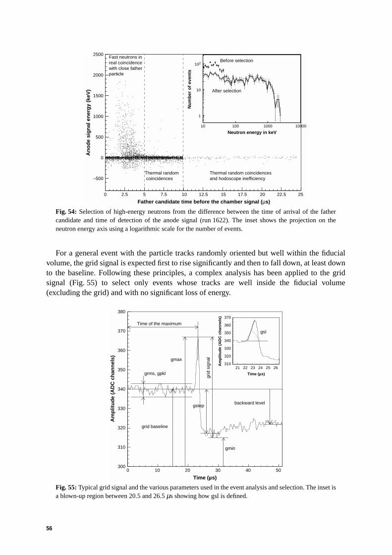
56

Fig. 54: Selection of high-energy neutrons from the difference between the time of arrival of the fathercandidate and time of detection of the anode signal (run 1622). The inset shows the projection on theneutron energy axis using a logarithmic scale for the number of events.

For a general event with the particle tracks randomly oriented but well within the fiducialvolume, the grid signal is expected first to rise significantly and then to fall down, at least downto the baseline. Following these principles, a complex analysis has been applied to the gridsignal (Fig. 55) to select only events whose tracks are well inside the fiducial volume(excluding the grid) and with no significant loss of energy.

Fig. 55: Typical grid signal and the various parameters used in the event analysis and selection. The inset isa blown-up region between 20.5 and 26.5 µs showing how gsl is defined.

Neutron energy in keV

1

10

102

10 100 1000 10000

–500

0

500

1000

1500

2000

2500

0 2.5 5 7.5 10 12.5 15 17.5 20 22.5 25

Father candidate time before the chamber signal (µs)

An

od

e si

gn

al e

ner

gy

(keV

)

Thermal random coincidences

Thermal random coincidencesand hodoscope inefficiency

Fast neutrons inreal coincidencewith close fatherparticle

Nu

mb

er o

f ev

ents

Before selection

After selection

grid

sig

nal

grid baseline

backward level

gmax

gmin

Time of the maximum

Time (µs)

Am

plit

ud

e (A

DC

ch

ann

els)

300

310

320

330

340

350

360

370

380

0 10 20 30 40 50

Time (µs)

Am

plit

ud

e (A

DC

ch

ann

els)

gsl

310

320

330

340

350

360

370

21 22 23 24 25 26

gstep

grms, gpkl

57

The two vetoes collect signals only if a fraction of the ionization is produced outside thefiducial volume. The presence of any significant signal in these channels indicates thepossibility of incomplete signal collection on the anode channel. A more detailed descriptionof the event selection criteria can be found in Ref. [54].

5.3.4 Calibration of the counter with monochromatic neutrons and simulation of thedetector response to neutrons

The 3He counter response to monoenergetic neutrons was measured in the calibrationexperiments performed in the CEN-Bordeaux-Gradignan Van de Graaff accelerator. In theseexperiments a monochromatic proton beam was sent on thin targets of tritium and 7Li. In thetargets the (p,n) reaction produces a monochromatic neutron beam (for a fixed angle withrespect to the proton beam). The counter was illuminated with these neutron beams at zerodegree and the response function was directly measured (Fig. 56).

Fig. 56: Detector response to a monochromatic neutron beam of 2014 keV at the CEN-Bordeaux-Gradignan van de Graaff accelerator.

It was also possible to compute, from the Bordeaux calibration, the efficiency of thedetector in the (n,p) peak as the number of signals for a given neutron fluence and to comparewith the quasitransparent approximation for the detector response (Fig. 57). In thisquasitransparent approximation, the detector efficiency is obtained as the product of the3He(n,p) reaction cross-section, times the total number of 3He nuclei in the fiducial volume,times the probability for the event to be accepted by the selection cuts (mainly the geometricalefficiency), times the probability of collection of the complete ionization charge released in thechamber.

The error bars in Fig. 57 correspond only to the statistical fluctuations. In addition, theuncertainties on the proton intensity (5%), the exposure time (2%), the production reaction

0

50

100

150

200

250

300

350

400

450

500 1000 1500 2000 2500

Proton energy: 2.8 MeV Target: 3HNeutron energy: 2.014 MeV

MC

Data

Signal — 764 keV (keV)

Co

un

ts

Epithermal peak

3He elastic scattering

3He elastic scatteringanisotropy H from CH4

elastic scattering

3He(n,p)3H

58

cross-section (2.5%), the thickness of the (3H and 7Li) targets (2%), the effect of the positionof the 3He counters with respect to the targets (8%), and the possible dead time (2%) produce atotal systematic uncertainty on the detector efficiency calibration of 10%. The combination ofthe statistical and systematic errors add from 10 to 15% to peak efficiency uncertainties.Similar considerations apply to the uncertainties on the convolution matrix.

Fig. 57: (n,p) peak efficiency of the 3He counter versus the neutron energy.

5.3.5 Detector resolution

As already mentioned when describing the electronic chain, the thermal noise in thepreamplifiers is the largest component in chamber resolution. Using electronic pulsescorresponding to 25 500 electrons (equivalent to 764 keV) injected into the preamplifier input,the resolution is measured to be 4.9% (FWHM).

The actual resolution of the chamber obtained with the help of an 241Am-Be (alpha,n)neutron source, after thermalizing the neutrons by surrounding the counter with 10 cm ofparaffin and screening against background neutrons with a thick layer of B4C (~ 5 cm) is 5.1%(FWHM), confirming that the resolution is dominated by the electronics.

During the actual data taking at the TARC experiment the resolution obtained by fitting thethermal peak with a Gaussian function is typically 5.9% (FWHM).

5.3.6 TARC experimental data set

A secondary PS beam [17] collected behind a target hit by the 26 GeV protons from the PSprovided typical pulses of 5000 to 10 000 particles (2.5 GeV/c), during a 400 ms spill, every14.4 s. A time-of-flight system was able to identify protons with 5σ separation but it was notpossible to identify pions from other light particles.

5.3.7 Monte Carlo simulation of the experiment

The full flux measurement experiment with the 3He ionization counter has been simulatedcombining the standard TARC simulation with the detailed detector simulation.

5.3.8 Fluence determination

For each position the collected signal spectra have been computed and normalized to thebeam intensity. Because of the complex response function of the 3He ionization detector tomonoenergetic neutrons, the fluence energy spectra cannot in general be obtained with highprecision, by simple division of the observed signal spectra by the counter efficiency. A

0

0.001

0.002

0.003

0.004

0.005

0.006

0.007

0.008

0.009

0.01

0 250 500 750 1000 1250 1500 1750 2000 2250

Neutron energy (keV)

Eff

icie

ncy

[co

un

ts/(

n/c

m2 )

]Experimental (n,p) peak efficiency

Transparent approx.(n,p) peak efficiency

59

deconvolution process is required. However, it should be noted that given the very rapidlydecreasing flux with increasing energy in the high-energy range in TARC, the error on thedirect flux calculation method can be acceptable for some positions and energy ranges.

Both methods have been used for the analysis of the TARC data as both, after smallcorrections, provide measurements with reduced and different systematic uncertainties,resulting in complementary information.

The simplest method to extract an estimate of the fluence from the signal, that we shall callthe peak efficiency method, consists of dividing, bin by bin, the histogram of signal amplitudesby the detector efficiency in the (n,p) peak (Fig. 57), after applying a small correctiondependent on the detector position. In the direct peak efficiency, for each energy bin we ignorethe contributions from elastic collisions of neutrons at higher energies resulting in an energydeposited corresponding to the bin under study. At TARC, the fluence decreases very steeply athigh energies and, as a consequence, the fraction of signals in a given energy bin coming fromneutrons with energies inside the same energy bin, through direct (n,p) reaction, is very highfor energies sufficiently low (typically below about 2 MeV) (Figs. 58 and 59). The fraction of(n,p) signals is, within errors, larger than 80% for all positions. An average energy-independentcorrection factor has been computed to take into account this difference, for each individualmeasurement position. The values for the corrections are in all cases smaller than 10% and themaximum systematic error left from this analysis method is also 10% (much smaller at farpositions).

The second method used to extract the fluence is what we call the deconvolution method. Itis described in detail in Ref. [54]. It is an attempt to take into account additional (n,p)contributions coming from recoiling nuclei produced by neutron elastic scattering mainly onhydrogen (contained in methane) and on 3He.

Figures 58 and 59 show the ratios, computed by Monte Carlo simulation, between signalsproduced in a specific energy bin by the neutrons with less than 2.4 MeV with respect to thecomplete neutron spectra. The ratio is very close to 1 for low neutron energies but can be aslow as 80% for neutron energies close to 2 MeV. Similarly to what was done in the firstanalysis method, an energy-independent correction factor has been computed for eachindividual position. This correction is again always smaller than 10% and the residualsystematic uncertainty is also smaller than 10%.

One additional consequence of both analysis methods is that the fluence can only becomputed with small uncertainties up to a maximum energy varying for each measuringposition. In any case, the statistics available at higher energies is very small and the statisticalerrors prevent any evaluation of the neutron fluence, above ~ 2 MeV. The systematic errors onthe fluence measurements are estimated to be 16 to 18%.

The validity of these methods of fluence extraction from the signal histograms has beenchecked with the full TARC Monte Carlo simulation.

Figure 60 shows the measured neutron fluence energy spectra at different positionsextracted from the signal histogram associated to proton-generated neutrons, using the twoanalysis methods and compared with the direct Monte Carlo predictions for those positions.The error bars include both the statistical and the systematic error. A generally good agreementis found at low energies, that extends up to 1.5 MeV for positions not too close to the spallationcascade, whereas for closer positions the measurements indicate larger neutron fluences at highenergies than what was predicted by the Monte Carlo simulation.

60

Fig. 58: Fraction of (n,p) signals in all events and fraction of signals (all n,p included) from neutrons ofenergy lower than 2.4 MeV for several positions in instrumentation hole 3 obtained from our Monte Carlosimulation (close to the centre of the lead volume where the neutron energy spectrum is harder).

Fig. 59: Fraction of (n,p) signals in all events and fraction of signals (all n,p included) from neutrons ofenergy lower than 2.4 MeV for several positions in the instrumentation holes 10, 7, and 8 obtained fromour Monte Carlo simulation (close to the centre of the lead volume where the neutron energy spectrum isharder).

0

0.2

0.4

0.6

0.8

1

Rat

ios

Ratio (n,p) / Total Ratio (E<2.4MeV)/Total

Ratio (n,p) / Total Ratio (E<2.4MeV)/Total

0

0.2

0.4

0.6

0.8

1

Rat

ios

Ratio (n,p) / Total Ratio (E<2.4MeV)/Total

0

0.2

0.4

0.6

0.8

1

Rat

ios

0 1000 2000 3000

Ratio (n,p) / Total Ratio (E<2.4MeV)/Total

0

0.2

0.4

0.6

0.8

1

Rat

ios

Hole 3; z = +37.5 cm Hole 3; z = –22.5 cm

Hole 3; z = –7.5 cm Hole 3; z = +7.5 cm

Energy (keV) 0 1000 2000 3000

Energy (keV)

0 1000 2000 3000Energy (keV)

0 1000 2000 3000Energy (keV)

0

0.2

0.4

0.6

0.8

1

Rat

ios

0

0.2

0.4

0.6

0.8

1

Rat

ios

0

0.2

0.4

0.6

0.8

1

Rat

ios

0

0.2

0.4

0.6

0.8

1

Rat

ios

0 1000 2000 3000Energy (keV)

0 1000 2000 3000Energy (keV)

0 1000 2000 3000Energy (keV)

0 1000 2000 3000Energy (keV)

Ratio (n,p)/Total Ratio (E<2.4MeV)/Total

Ratio (n,p)/Total Ratio (E<2.4MeV)/Total

Ratio (n,p)/Total Ratio (E<2.4MeV)/Total

Ratio (n,p)/Total Ratio (E<2.4MeV)/Total

Hole 10; z = +7.5 cm Hole 10; z = +37.5 cm

Hole 7; z = +7.5 cm Hole 8; z = +7.5 cm

61

Fig. 60: Measured neutron fluence spectra produced by 2.5 GeV/c protons, at different positions in theTARC lead assembly.

For positions sufficiently far from the spallation cascade, 40 cm or more, there is goodagreement between data and Monte Carlo (Fig. 61). On the other hand, for close positions theagreement is good up to 200 keV, getting worse for higher energies (Fig. 61). In this last case

1

10

102

Energy (keV)

1

10

102

1

10

102

10

102

0 500 1000Energy (keV)

0 500 1000

Energy (keV)0 500 1000

Energy (keV)0 500 1000

Direct MC fluence

Data fluence fr. Efficiency

Data fluence Deconvoluted

Protons Protons

ProtonsProtons

Flu

ence

(n

/cm

2 /eV

) fo

r 10

9 p

roto

ns

Flu

ence

(n

/cm

2 /eV

) fo

r 10

9 p

roto

ns

Flu

ence

(n

/cm

2 /eV

) fo

r 10

9 p

roto

ns

Flu

ence

(n

/cm

2 /eV

) fo

r 10

9 p

roto

ns

Direct MC fluence

Data fluence fr. Efficiency

Data fluence Deconvoluted

Direct MC fluence

Data fluence fr. Efficiency

Data fluence Deconvoluted

Direct MC fluence

Data fluence fr. Efficiency

Data fluence Deconvoluted

Hole 10; Z = +7.5 cm

Hole 3; Z = +37.5 cm Hole 3; Z = -22.5 cm

Hole 10; Z = +37.5 cm

62

the experimental values for the fluence are always larger than the neutron fluence from theMonte Carlo. One possible explanation for part of this difference is the fact that the positionswhere there are discrepancies are deeply inside the spallation cascade and this has twoconsequences. First, some very high energy neutrons (E > 20 MeV) are present but notincluded in the Monte Carlo estimation of the signals histogram, and consequently in therequired corrections for the analysis methods. This is because neutrons above 20 MeV aretreated in the FLUKA step, and their contribution to the fluence is not retained. Second, atthese positions, in addition to neutrons, there is also a substantial fluence of high-energyphotons and charged particles. The detector is designed to have a high rejection factor forsignals coming from these particles, but residuals will contribute to the observed differences.

Fig. 61: Distribution of the neutron fluence as a function of distance with respect to the center of the TARClead volume, at different energies measured by the 3He ionization counter. The minus signs indicatepositions at z < 0.

5.3.9 Conclusion

An innovative system of signal collection has allowed us to use the full anode and gridsignal shapes for the data analysis, achieving enhanced rejection of unwanted events such aspile-ups, events produced outside the fiducial volume, and events with incomplete energycollection.

The energy spectra of the neutron fluence were measured in the range from a few tens ofkeV up to about 1.5 MeV. The precise range of reliable measurements depends on the hardnessof the neutron fluence spectra and consequently is a function of the distance from themeasurement position and the spallation target.

As the statistics is generally limited we tried to combine the signals coming from protonswith those coming from pions [54]. This is possible because of the very similar shape of theneutron fluence energy spectra produced by the two types of particles with the same nominalmomentum at TARC (2.5 GeV/c). This is confirmed both by our experimental data and by theMonte Carlo simulation. However, the very large uncertainty on the pion beam intensityprevents this merging of data from being quantitatively significant.

0

20

40

60

80

100

120

140

160

–40 –20 0 20 40 60 80 100 120 140

Distance to the centre (× Z sign)

Flu

ence

(n

/cm

2 /eV

) fo

r 10

9 p

roto

ns

Data 84 keVMC 84 keV

Data 180 keVMC 180 keV

Data 480 keVMC 480 keV

Data 950 keVMC 950 keV

(cm)

63

In spite of the many difficulties in performing such measurements, a reasonable agreementis found with our Monte Carlo predictions both for the neutron flux energy and spacedistributions, especially good for positions outside the spallation cascade core extending over40–50 cm from the centre of the cascade.

The 3He ionization counter measurements are unique because they cover the energy regionwhere the shape of the fluence energy distribution changes very rapidly and is very sensitive tothe properties of the spallation process (Fig. 62). This gives us at the same time a direct test ofthe neutron transport in the energy region dominated by the lead capture resonances.

Fig. 62: Distribution of the neutron fluence versus its energy measured by the 3He ionization detector inthe TARC lead volume (hole 10, z = +7.5 cm). The other data come from 3He scintillation and 6Li/233Udetectors. The histogram is the Monte Carlo simulation. All data were taken with protons of 2.5 GeV/cmomentum.

5.4 High-energy neutrons with activation methods

5.4.1 Fissions in 232Th, and 237Np

The distribution of fission rates in the TARC lead volume was measured using fissionablematerials (232Th, Unatural,

235U, 239Pu and 237Np) in close contact with Lexan track-etchdetectors, which can detect the produced fission fragments. Integral measurements of thehigh-energy neutron fluence (En > 1.4 MeV) obtained from fission on 232Th, provide the mostsignificant additional check of the neutron fluence at high energy.

Only 232Th and 237Np measurements are reported here. The details of the technique used aswell as the other measurements can be found in Ref. [55].

The fission cross-section of 232Th is negligible for neutrons with energies En < 1.4 MeV butbecomes significant for neutrons with higher energies. This makes the 232Th a good tool tostudy the integral neutron fluence for energies above 1.4 MeV. Our data are in excellentagreement with the Monte Carlo prediction (Fig. 63).

For 237Np this is not the case (Fig. 64) pointing out a potential problem with the 237Npfission cross-section database.

The error on the simulation was estimated to be 10% coming mainly from the Monte Carlosimulation statistical error and from the uncertainty on cross-section data from differentdatabases. The second stage of TARC Monte Carlo simulation processes only neutrons withenergy E < 19.6 MeV. However, there is a small contribution of neutrons with higher energies(E > 19.6 MeV) in the case of 232Th and 237Np which was calculated in the FLUKA stage and

10–2 10–1 1 10 102 103 104 105 106 107

10–2 10–1 1 10 102 103 104 105 106 107

Neutron energy (eV)

E×d

F/d

E (

neu

tro

n/c

m2 f

or

109

pro

ton

s)

3He Scintillation

6Li/233U Detectors

3He Ionization

Monte Carlo

107

106

105

104

103

107

106

105

104

103

64

found to represent typically 12% and 10% of the neutrons with energy 1.4 MeV < En < 19.6 MeV,at z = 7.5 cm in holes 3 and 10, respectively. For 232Th the average fission cross-section of0.27 b for neutrons with energy En > 1.4 MeV (used as a reference for the fluencemeasurements of neutrons with En > 1.4 MeV) and the cross-section from the ENDF/B-VIdatabase were compared (Fig. 63). Both gave similar results within the above errors althoughthe Monte Carlo results using the ENDF/B-VI database are slightly underestimated, since theydo not include neutrons above 19.6 MeV.

Fig. 63: Measurement of fission rates in 232Th as a function of distance from the centre of the lead volume,in hole 3 (black squares), in other holes (stars) and comparison with the TARC Monte Carlo simulationusing ENDF/B-VI (open circles) and using a step function cross-section (0.27 b) (open triangles).

Fig. 64: Measurement of fission rates in 237Np as a function of distance from the centre of the lead volume,in hole 3 (black squares) and comparison with the Monte Carlo simulations using ENDF/B-VI (opencircles), JENDL-3.2 (open triangles).

In the case of 237Np the fission rates predicted by ENDF/B-VI and JENDL-3.2 showdifferences ranging from 11% near the centre of the lead volume to a factor 3 larger forJENDL-3.2 at a distance 1.5 m from the centre. This indicates large inaccuracies in the 237Npfission cross-section (Fig. 65). However, this does not explain the discrepancy with our datawhich are a factor 2 higher than the prediction (Fig. 64).

0

0.001

0.002

0.003

0.004

0.005

0.006

0.007

0.008

0.009

0.01

—150 —100 —50 0 50 100 150

Distance to centre (cm)

Fis

sio

ns

/ µg

/ 10

9 p

roto

ns

232Th

0

0.05

0.1

0.15

0.2

0.25

0.3

0.35

0.4

—150 —100 —50 0 50 100 150

Distance to centre (cm)

Fis

sio

ns

/ µg

/ 10

9 p

roto

ns

237Np

65

Fig. 65: The fission cross-section of 237Np from the JENDL-3.2 (full line) and ENDF/B-VI (dotted line)data libraries as a function of neutron energy.

In conclusion, Lexan is an integral fission fragment detector. It measures fission fragmentsproduced in the converter by the whole energy spectrum of incident neutrons. However, owingto the properties of the fission cross-section of the 232Th converter and its neutron energythreshold of about 1.4 MeV for fission, fluences of fast neutrons with energy greater than1.4 MeV can be measured using the fission measurements with 232Th (see Ref. [55]). Thesefast neutron fluences measurements are in agreement with the corresponding Monte Carlocalculations, providing an important check of the high energy component of the neutronfluence, which in addition has important implications in the design parameters of the EnergyAmplifier (fast neutron damage to structural material).

Further studies of the neutron fluence at high energies were performed with 12C(n,2n)11Cand 12C(n,3n)10C reactions. This was done using the carbon shuttle in the rabbit measurement(Section 7.1). The reader is referred to Ref. [8] for a complete description of thesemeasurements.

5.5 General conclusion on neutron fluence measurements

We have used several techniques (Fig. 66) in TARC to measure neutron fluences over thedesired energy range from thermal to MeV neutrons.

The 6Li/233U detectors and the 3He detector in the scintillation mode cover the neutronenergy range from thermal up to about 100 keV and the 3He ionization detector covers thehigher energy range from 10 keV to 2 MeV. These differential measurements werecomplemented by measurements at specific neutron energies with triple-foil activationmethods. Several additional cross-checks of the neutron fluence were performed, outside theenergy range covered by the electronic detectors both at low energies (< 0.5 eV) usingthermoluminescence techniques and at high energies (> 1.4 MeV) using fission measurementin 232Th. At higher energies threshold reactions [12C(n,2n)11C (En > 22 MeV) and12C(n,3n)10C (En > 34 MeV)] have also been studied.

In all cases, our measurements are found to be in very good agreement with our simulation(Fig. 67). We find also, in particular with the fission measurements in 232Th, that the spatialdistribution of the high-energy component of the neutron fluence shows a significant

10—5

10—4

10—3

10—2

10—1

100

101

102

10—2 10—1 100 101 102 103 104 105 106 107 108

ENDF/B-VI

JENDL-3.2

Neutron Energy (eV)

Cro

ss-s

ecti

on

(b

arn

)

66

forward–backward asymmetry and dies away quickly (within 50 cm from the centre of thecascade generated by the beam protons) which is a very useful practical consideration for thedesign of the EA where fast-neutron damage in structural materials must be minimized.

The data corresponding to Fig. 67 are given in the Appendix, so that they can be useful forbenchmaking of future simulation codes.

Fig. 66: Illustration of the energy ranges covered by the different detector techniques used in TARC tomeasure neutron fluences.

We can use the simulation to investigate further the behaviour of neutrons in lead. We can,for instance, switch off the neutron capture process in the simulation and observe themodification of the neutron fluence (Fig. 68). We find that indeed, in our lead, the effect ofcaptures is relatively small, down to neutron energies of 1 eV. For instance, the fluence(dF/d[ln(E)] decreases only by a factor 10 from 1 MeV to 1 eV, while if we switch off leadcaptures, this factor is reduced to 5. This remaining decrease in fluence is due in part to the factthat the lead volume is not infinite and also to a diffusion effect well accounted for in the Fermiage theory.

We have obtained a large coherent set of neutron fluence measurements, with redundantmethods especially in the energy range below ~ 10 keV where we want to use the ARCmethod. This is the first important element in our demonstration of the efficiency of the ARCeffect confirming the high transparency of lead over the whole neutron energy range. The factthat the simulation of the neutron fluence at any point within the TARC lead volume agreeswith the data, confirms that both the spallation process (FLUKA) and the neutron diffusion andtransport (cross-sections) are well described, and constitutes a precise validation of the overallsimulation chain developed by our group (see Section 3).

Another interesting aspect of these neutron fluence measurements is that they provide acheck of the complete chain of processes from neutron production by spallation to neutrontransport until capture or escape from the lead assembly. If we assume that neutron transport isknown with good accuracy (~ 10%, see Section 3), then our measurements provide a check ofthe spallation process. We can note that the number of neutrons produced and transporteddown to 19.6 MeV is found to be 98 for a proton momentum of 3.5 GeV/c.

10–2 10–1 100 101 102 103 104 105 106

Neutron energy (eV)

115In

107

197AuTLD

Si Detectors: 6Li/233U

3He (scintillation)

3He (ionization)

Ele

ctro

nic

det

ecto

rs

Var

iou

sac

tiva

tio

n t

ech

niq

ues

Etched trackdetectors

237Np

232Th

186W

12C(n,2n)

12C(n,3n)

108

Thermal

67

Fig. 67: a) Example of TARC measurements of the neutron fluence. E × dF/dE is shown as a function ofneutron energy, from 2.5 and 3.57 GeV/c protons in hole number 10 (z = 7.5 cm, at a distance of 45.6 cmfrom the centre of the lead volume). The Monte Carlo predictions are shown as histograms. The data arefrom 6Li/233U detectors (open circles), 3He in the scintillation mode (full circles) and 3He in the ionizationmode (full squares). The error bars include both statistical and systematic errors added in quadrature;b) Variation of the neutron fluence as a function of distance from the centre of the lead volume (the minussign indicates negative z positions). dF/dE is shown for a few selected energy bins. The Monte Carlopredictions are shown as lines obtained from a Gaussian fit to Monte Carlo points. The data are shown withthe same convention as in part (a) with, in addition, data from triple-foil activations shown as full triangles.

b)

–200 –150 –100 –50 0 50 100 150 200

0.10 eV

1.46 eV (In)

5 eV (Au)

18 eV (W)

100 eV

480 eV1 keV

10 keV

180 keV

Distance to the centre of lead volume (cm)

dF

/dE

(n

/cm

2 /eV

/109

pro

ton

s)

6LiF/233U Detectors Monte Carlo

3He Scintillation Activation Foils

3He Ionization

10–2 10–1 1 10 102 103 104 105 106 107

10–2 10–1 1 10 102 103 104 105 106 107

102

103

104

105

106

102

103

104

105

106

103

104

105

106

107

108

109

1010

101

102

103

104

105

106

107

108

Neutron energy (eV)

E×d

F/d

E (

neu

tro

n/c

m2

for

109

pro

ton

s o

f 3.

57 G

eV/c

)

E×d

F/d

E (

neu

tro

n/c

m2

for

109

pro

ton

s o

f 2.

5 G

eV/c

)

scale

scale

3.57 GeV/c

2.5 GeV/c

3He Scintillation

6Li/233U Detectors

3He Ionization

Monte Carlo

a)

68

Fig. 68: Comparison of the neutron fluence in hole number 10, z = +7.5 cm, with and without neutroncaptures in lead.

6 Neutron Capture Cross-Section Measurements as a Function of Energy

6.1 Detecting neutron capture with a CeF3 detector

The prompt γ-rays of the cascade following a neutron capture are detected using a CeF3scintillator coupled to a quartz window photomultiplier (Philips XP–2020Q). The CeF3 hasbeen chosen because the neutron capture cross-section in this material is very small and itsscintillation light has fast decay-time constants (5 and 30 ns). In practice, two detectors wereassembled with scintillators cross-sections of 2 × 2 cm2 and thicknesses of 2 mm and 4 mmrespectively. The scintillator (Fig. 69) is coupled to the photocathode by a film of opticalgrease, and a thin 5 µm aluminium foil is used as light reflector on the opposite face. The lighttightness was achieved with black adhesive tape. The target, usually a metallic foil, ismaintained on the scintillator with two very small pieces of tape and is covered by analuminium foil. The output signal from the photomultiplier is amplified by a fast amplifier(integration time of 0.5 µs), whose output is encoded by an 8-bit flash-ADC (8192 channels,0.1 µs/channel). An example of a flash-ADC record for a tantalum target is given in Fig. 70.

Immediately after the arrival of the proton beam burst, a high reaction rate is produced inthe detector which saturates the photomultiplier for a few microseconds. Therefore, thecounting rate for times t < 5 µs is not reliably measured. This effect induces a limitation in ourmeasurements. Reliable data have been obtained only for neutron energies smaller than≈ 6 keV. As can be seen from Fig. 70, the counting rate was rather high and precisemeasurement of the single-pulse time distribution was not possible. We analysed the data byadding together all flash records, which turns out to be equivalent to a current integrationmethod.

The data processing is described in detail in Ref. [8]. A typical accumulated time spectrumobtained with our 99Tc sample is shown in Fig. 71.

104

105

106

107

10–3 10–2 10–1 1 10 102 103 104 105 106 107

Neutron energy (eV)

Flu

ence

(d

F/d

lnE

)

Simulated fluenceNo lead captures

Simulated fluenceWith lead captures

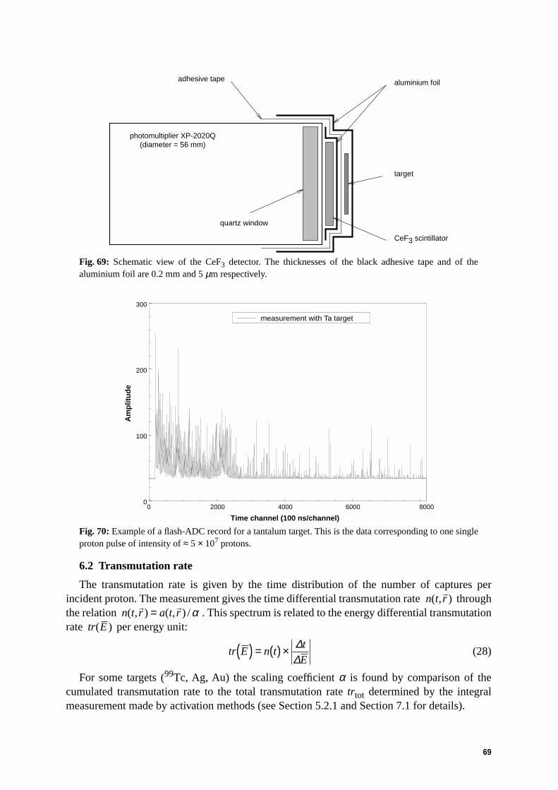
69

Fig. 69: Schematic view of the CeF3 detector. The thicknesses of the black adhesive tape and of thealuminium foil are 0.2 mm and 5 µm respectively.

Fig. 70: Example of a flash-ADC record for a tantalum target. This is the data corresponding to one singleproton pulse of intensity of ≈ 5 × 107 protons.

6.2 Transmutation rate

The transmutation rate is given by the time distribution of the number of captures perincident proton. The measurement gives the time differential transmutation rate throughthe relation . This spectrum is related to the energy differential transmutationrate per energy unit:

(28)

For some targets (99Tc, Ag, Au) the scaling coefficient α is found by comparison of thecumulated transmutation rate to the total transmutation rate trtot determined by the integralmeasurement made by activation methods (see Section 5.2.1 and Section 7.1 for details).

adhesive tape

target

CeF3 scintillator

aluminium foil

quartz window

photomultiplier XP-2020Q(diameter = 56 mm)

0 2000 4000 6000 8000

Time channel (100 ns/channel)

0

100

200

300

Am

plit

ud

e

measurement with Ta target

n t r( , )r

n t r a t r( , ) ( , ) /r r= α

tr E( )

tr E n tt

E( ) = ( ) × ∆

∆

70

; (29)

if trtot is determined from activation measurements, then α can be obtained.

For the other targets, the scaling coefficient α’s were found by adjustment of theexperimental results on the Monte Carlo calculation using the JENDL database and the fullexperimental set-up description.

Fig. 71: Experimental time spectra obtained for technetium. The upper figure shows spectra taken with andwithout the target sample. The lower figure shows the signal spectrum obtained by subtraction of the twoupper spectra.

6.3 Apparent cross-section

It has been shown in Section 5.2.1.2 that the reaction rate can be written as:

(30)

where the neutron flux at a point in the target volumeV, located around the position in thelead is defined as:

. (31)

In this equation the correlation function M(E,t) is a normalized probability

.

Using the energy–time relation, Eq. (31) can be written in an equivalentmanner:

tr n t t a t ttot d d= = ∫∫ ( ) ( )1α

0 200 400 600 800

0 200 400 600 800

Time (µs)

0

500

1000

1500

Target minus background

0

500

1000

1500

2000

2500

99Tc targetbackground

Cu

mu

late

d a

mp

litu

des

for

109

pro

ton

s

∆ ∆ ∆n t r n t r tN

Vx F t x M E t E E( ) ), ( , d , , ( )dtarget

target volume

= = ( ) ( )∫∫ σ

rx

rr

φ E t x t F t x M E t, , , ,( ) = ( ) ( )∆ ∆

M E t E,( ) =∞

∫0

1d

E t K t t( ) /= +( )02

71

. (32)

With these definitions, Eq. (30) reads:

(33)

or, since the fluence can be considered as constant over the volume of the target

. (34)

Because of self-screening effects, this complete formulation cannot be avoided. The actualmean fluence can be significantly affected by the presence of the targetitself. Then we define an apparent cross-section by the following equation:

(35)

where is the unperturbed fluence measured at position . Thisapparent cross-section would be the quantity defined in Section 5, inthe case of a very thin target without any self-screening effect. In this apparent cross-section,both self-screening effects and averaging by the M(E,t) function, are included. Using thisformulation the unperturbed fluence measured by 6Li/233U or 3He counters is used toextract . The apparent cross-section can then be written as:

(36)

6.3.1 Absolute values

To obtain the apparent cross-sections given by Eq. (36) one assumes explicitly that theefficiency, which enters the α coefficient, is constant over the observed neutron energy rangefor a given target. This hypothesis which implies that the γ cascade is fairly independent of theneutron energy seems rather reasonable, since between few keV and 0.1 eV the neutronangular momentum with respect to the target nucleus remains mostly L = 0, the same excitedstates of the compound nucleus are formed, and therefore the γ cascade can be supposed to beindependent of neutron energy. Typical energies of the cascade gammas are of the order of 1 to2 MeV; therefore, our small scintillator (2 × 2 × 0.2 cm3) has a low intrinsic efficiency fordetecting these gamma rays, but it is more efficient for the low-gamma energies ending thecascade. Hence we expect the efficiency to be independent of the neutron energy (0.1 eV tofew keV) but dependent on the type of target element. As a consequence neither the efficiencynor the α coefficient can be known simply in an absolute manner.

So the CeF3 measurements alone will determine only the energy profiles of transmutationrates, or apparent cross-sections which are sample-dependent. For the absolute values of 99Tctransmutation rates or σapp(E) we will normalize the measured relative values using theactivation measurements made with the rabbit system.

6.3.2 Error analysis

In Eq. (36), can be replaced by . Then the errors on σapp can becalculated as follows:

φ E t x t F E t x M E E t, , = ,( ) ( )( ) ( )( )∆ ∆ ,

∆ ∆n t r

N

Vx F E t x E( , ) ,= ( )∫target

target volume

d ( ) ( )σ

∆ ∆n t r

N

VV F E t r E( , ) ,= ( )target ( ) ( )σ

∆ ∆F E x f E x E( (, ) , )=

∆ ∆n t r N F E r E( , ) ( , ) ( )

r r= target app0 σ

∆F E r f E r E0 0( , ) ( , )r r= d

rr

σ σ= ∫ M E t E E( , ) ( )d

f E r0( , )r

σapp E( )σ

αapptarget target, ) , )

En t r

N F E r

a t r

N f E r

t

E( ) = =∆

∆∆∆

( , )(

( , )(0 0

∆ ∆t E/ ( ) ( )t t K+ 03 2

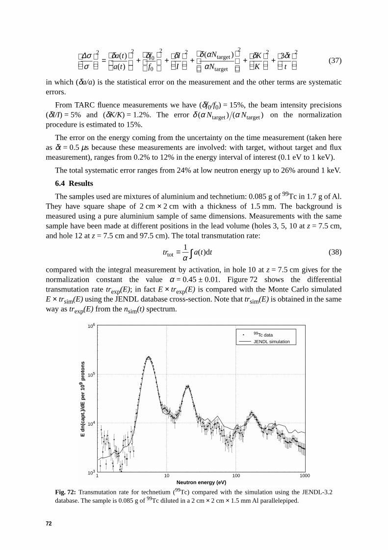
72

(37)

in which (δa/a) is the statistical error on the measurement and the other terms are systematicerrors.

From TARC fluence measurements we have (δf0/f0) = 15%, the beam intensity precisions(δI/I) = 5% and (δK/K) = 1.2%. The error on the normalizationprocedure is estimated to 15%.

The error on the energy coming from the uncertainty on the time measurement (taken hereas δt = 0.5 µs because these measurements are involved: with target, without target and fluxmeasurement), ranges from 0.2% to 12% in the energy interval of interest (0.1 eV to 1 keV).

The total systematic error ranges from 24% at low neutron energy up to 26% around 1 keV.

6.4 Results

The samples used are mixtures of aluminium and technetium: 0.085 g of 99Tc in 1.7 g of Al.They have square shape of 2 cm × 2 cm with a thickness of 1.5 mm. The background ismeasured using a pure aluminium sample of same dimensions. Measurements with the samesample have been made at different positions in the lead volume (holes 3, 5, 10 at z = 7.5 cm,and hole 12 at z = 7.5 cm and 97.5 cm). The total transmutation rate:

(38)

compared with the integral measurement by activation, in hole 10 at z = 7.5 cm gives for thenormalization constant the value α = 0.45 ± 0.01. Figure 72 shows the differentialtransmutation rate trexp(E); in fact E × trexp(E) is compared with the Monte Carlo simulatedE × trsim(E) using the JENDL database cross-section. Note that trsim(E) is obtained in the sameway as trexp(E) from the nsim(t) spectrum.

Fig. 72: Transmutation rate for technetium (99Tc) compared with the simulation using the JENDL-3.2database. The sample is 0.085 g of 99Tc diluted in a 2 cm × 2 cm × 1.5 mm Al parallelepiped.

∆σσ

δ δ δ δ αα

δ δ

=

+

+

+

+

+

2 20

0

2 2 2 2 23a t

a t

f

f

I

I

N

N

K

K

t

t

( )( )

( )target

target

δ α α( ) ( )N Ntarget target

tr a t ttot d= ∫1α

( )

1 10 100 1000

Neutron energy (eV)

103

104

105

106

E d

n(c

apt.

)/d

E p

er 1

09 p

roto

ns

99Tc data

JENDL simulation

73

The cross-section data (Fig. 73) are not extrapolated to zero thickness. An estimation of thiscorrection would give a value 50% higher for the larger resonance at 5.58 eV, 18% for theresonance at 22.3 eV and no significant correction for other energies. We checked that thecross-section data are, as expected, independent of position. The relative systematic error is, onaverage, in the order of 15–20%.

Note that the general shape of the experimental apparent cross-section is in good agreementwith the full Monte Carlo simulation using the JENDL cross-section (Fig. 73). Our results arecompared with the previous measurement (which is extrapolated to zero thickness) ofJ.C. Chou and H. Werle [39] in Fig. 74.

Fig. 73: Averaged TARC (n,γ) apparent cross-section for 99Tc compared with the simulation using theJENDL-3.2 database.

Fig. 74: Averaged TARC (n,γ) apparent cross-section for 99Tc compared with Chou and Werle’s data [39].

1 10 100 1000

Neutron energy (eV)

1

10

100

1000

Ap

par

ent

cro

ss-s

ecti

on

(b

arn

)

mean exp. apparent cross section for 99TcJENDL simulation hole 10; z = 7.5 cm

1 10 100 1000

Neutron energy (eV)

1

10

100

1000

Ap

par

ent

cro

ss-s

ecti

on

(b

arn

)

99Tc mean exp. cross sectioncross section from J.C. Chou at al.

74

These experimental results on the energy dependence of transmutation rates obtained (withonly 85 mg of 99Tc), normalized by the activation measurement (rabbit), give a quite completeexperimental check of the validity of the JENDL database neutron capture cross-section for99Tc. It implies also that the resulting simulation is validated in detail and gives strongconfidence in the simulation of other transmutation applications.

6.5 Evaluation of the 99Tc cross-section

We have evaluated the Geel data [56] using the SAMMY code [57] and found thatintegrating the neutron capture rate over the neutron energy range covered by the evaluation(0.7 to 617 eV) leads to a + 3% increase in the predicted number of captures when comparedwith JENDL-3.2, which is a small difference compared with the size of the errors quoted forinstance in the rabbit analysis. Therefore, we conclude that the new Geel data do not make anysignificant change in the various predictions of the number of captures on 99Tc in TARC (mostof the captures in TARC occur on the two main resonances of 99Tc).

We have corrected the apparent TARC cross-section for both the effect of the hydrogencontained in the plastic tape surrounding the photomultiplier tube and the effect of the 99Tcsample thickness (21.2 mg/cm2), using the SAMMY code. The sample thickness effect is mostsignificant at the two main capture resonances, at 5.6 eV and 22.3 eV where its magnitude is50% and 18%, respectively.

In both cases (JENDL-3.2 and GEEL) there is a good agreement with the cross-sectionsobtained by TARC (Fig. 75), within the estimated overall systematic error of about 25%. Eventhough it was not the purpose of TARC to measure cross-sections, the fact that good qualitycross-section data could be obtained from our studies of 99Tc transmutation is a check of thegeneral high quality of TARC data.

Fig. 75: Comparison of the TARC 99Tc(n,γ) cross-section data with an evaluation based on GEEL data andan evaluation based on the JENDL-3.2 data library. In both cases the lines correspond to the cross sectionsat 293 K and have been broadened for the slowing-down resolution (∆E/E ~ 12%).

Neutron energy (eV)

Cro

ss-s

ecti

on

(b

arn

)

GEEL

JENDL-3.2

TARC Data

1 10 102 103

1

10

102

103

75

6.6 Results for other targets

Apparent (n,γ) cross-sections for 181Ta, 197Au, natAg, and natIn targets have also beenmeasured and are reported in Ref. [8].

6.7 Conclusion

TARC has shown that the energy variation of the 99Tc (n,γ) transmutation cross-section canbe validated quite accurately with short measurement times and small quantities of material.The concept of transmutation by adiabatic resonance crossing is fully understood in a lowlethargy medium (lead). The self-shielding effect, which modifies the local flux inside thesample volume, and the flux perturbation due to the detector itself are well taken into accountby the Monte Carlo simulation.

The transmutation rate (tr) as a function of neutron energy was measured with a goodprecision using small samples of material. Reliable energy profiles have been obtainedbetween 1 eV up to 1 keV which represents more than 80% of the total tr. These datacombined with activation measurements provide absolute apparent cross-section measurementfor given samples. From a more general point of view, this method can be considered as verywell adapted for checking the validity (or non-validity) of present database cross-sections fortransmutation calculation. Finally, it can be stressed that in this experiment neutron fluencesand transmutation rates have been measured independently and both agree well with ourMonte Carlo simulations.

7 Test of Transmutation of Long-Lived Fission Fragments

7.1 99Tc rabbit integral transmutation rate measurements

One of the main goals of the TARC experiment is the study of transmutation of Long-LivedFission Fragments (LLFFs) using Adiabatic Resonance Crossing (ARC). After havingdemonstrated that the neutron flux in the lead volume has the expected properties, we havemeasured directly the transmutation rate for the most important LLFFs in order to complete thedemonstration that ARC works effectively, choosing two LLFFs of major relevance: 99Tc and129I (which represent about 95% of the LLFF radiotoxicity). In a system such as the EnergyAmplifier (EA) [2], where the actinides from PWR spent fuel are incinerated, LLFFs such as99Tc and 129I generate the main contribution to the long-term radiotoxicity (> 500 years). Aspallation neutron, surviving the lead capture resonances, cannot miss a given resonanceenergy such as 5.6 eV in 99Tc. In its ‘adiabatic’ slowing down process, a neutron will sweep allenergies with very small steps of constant ∆E/E, until it is captured with high probability on an‘impurity’ with a high resonance in its capture cross-section, as is the case for 99Tc (Fig. 76).As already explained in Section 1 the TARC effect maximizes the efficiency of the process.

In the case of 99Tc the two main resonances at 5.6 eV and 22.3 eV correspond, because ofthe energy–time correlation (Section 4), to neutron captures occurring respectively 175 and87 µs (Fig. 76) after the arrival of the proton beam.

7.1.1 Motivation

By neutron capture the 99Tc (2.1 × 105 years half-life) becomes 100Tc (15.8 s half-life)which in turn decays into the excited states of 100Ru, finally stable. The ‘rabbit system’ methodconsists in evaluating the number of 99Tc nuclei transmuted by counting of the 100Tcde-excitation photons. Since the 99Tc itself is radioactive, and given the complex structure ofthe photon energy spectra produced by the irradiated 99Tc sample, we use a pair of

76

high-efficiency, High-Purity germanium (HPGe) detectors. They provide sufficient photonenergy resolution to identify and count the number of photons in each individual characteristicline. The two germanium counters provide redundancy of information allowing detailedsystematic studies. To reduce the radiation background and avoid damage to the HPGe by thefast neutrons present in the irradiation area, the sample is transferred to a remote countingstation by a pneumatic system (described in Section 7.1.2).

Fig. 76: 99Tc neutron capture cross-section as a function of neutron kinetic energy (from the JENDL-3.2database). The times from the arrival of the proton pulse corresponding to the two main capture resonancesare indicated.

7.1.2 Experimental set-up

A primary fast extracted proton beam with 2.75 GeV of kinetic energy (3.5 GeV/cmomentum) and an intensity of a few times 109 protons per pulse was used, with a repetitionperiod of 14.4 s. A proton pulse, incident on a large volume of lead, produces by spallation aneutron cascade. These spallation neutrons diffuse and thermalize inside the lead volume. A99Tc sample, contained in a transport shuttle (rabbit), is placed at different positions in the leadassembly, before and at least until 0.5 s after the beam arrives (long enough to make sure thatall spallation neutrons have been produced and captured or escaped from the lead). Some 99Tcnuclei will capture a neutron and become 100Tc, with a 15.8 s half-life. The shuttle is thentransferred by a pneumatic system to a measurement station (Fig. 77). This station consists oftwo large HPGe detectors inside a massive shielding system. The photons produced by thetransition from the 100Ru excited states (produced in 100Tc decay) to the ground state arecollected during most of the time interval between beam pulses (9 s out of 14.4 s). Each singlephoton or photon coincidence between the two germanium counters is registered in amplitudeand time by an appropriate DAQ system, which also registers the beam intensity for eachaccelerator beam shot and monitors the proper operation of the pneumatic system and thecorrect positioning inside the measurement station of the shuttle containing the sample. Afterthe measurement, the sample is sent back to the irradiation position, a fraction of a secondbefore the next beam shot arrives. This process is repeated until enough statistics are collected(typically 104 counts in the major photon peaks).

Neutron energy (eV)

10–5 10–3 10–1 101 103 105 107

Cro

ss-s

ecti

on

(b

arn

)

10–4

10–3

10–2

10–1

100

101

102

103

104

175 µs 87 µs

Thermal

Adiabatic Slowing Down

77

7.1.2.1 The pneumatic system

The pneumatic system consists of two ports, the irradiation (R) and the measurement (M)ports, connected by a 24 m long plastic tube (Fig. 77). Each port contains a set of threeelectromechanical valves, a couple of pressurized air reservoirs, specific pieces to define theposition of the shuttle containing the samples, and one optical sensor mounted on the tubeclose to the port.

Fig. 77: a) Schematic layout of the ‘rabbit’ system; b) View of the carbon fibre shuttle containing the 99Tcsample in the irradiation port; c) View of the gamma-ray detection station.

A specially designed electronic control box allows the state of each electrovalve to be setaccording to the signal received from the optical sensors, the pressure in the tube, or throughexternal commands. These commands can be provided either by a manual switch box or by theinput signal of the automatic controls.

The tube connecting the two ports is made of Polyamid 116 and has internal and externaldiameters of 10 mm and 12 mm, respectively. A couple of pressure sensors have also beeninstalled in the tube. The first one is an analogic pressure transducer, for calibration anddiagnostic purposes, and the second a digital sensor that produces a signal whenever thepressure in the tube crosses some predefined thresholds. The signals are used to control thepneumatic cycle and the values for these thresholds have been calibrated for each individualtransport shuttle. Typical values were of the order of 1.9 and 2.75 bar.

7.1.2.2 The sample irradiation shuttle

As already mentioned, the samples are transported by the rabbit between the irradiation andthe measuring ports inside a special shuttle. The function of this shuttle is to hold the sampleduring the transport, to position it at the two ports, and to provide the required safety in casethere is an unexpectedly strong collision of the shuttle with the stoppers at any of the two ports.

6. Rilsan, Polyamid 11, Hoses for fluids and gases - Stores catalogue CERN 38.40.30.612.4.

V1

V2V3

V6

V5

V4

Irradiation port

Lead block(not to scale)

Measurement port(2 germanium detectors)

15 cm Pb, 1cm Cu, 5 mm Al shielding

DR DMPR PM

SASA

SA SA

Total tube length: 24 mPS cycle 14.4 sMeasurement time 9 sTime at irradiation 2.5 sTravel times 1.0 to 1.4 s

5 bar 5 bar

4 bar 3.5 bar

R ≈ 70 cm

99Tc sample

Germanium detector

Acceleration loop

Shuttle

Pb+Cu+Alshielding

����

����

b)

a)

c)

���������

��

������

���������

������

����

��

TcO4K (0.206 g)Carbon Steel Lead

78

The length of the shuttle is 33.5 mm and the external diameter is 9.5 mm. The internal cylinderlength, where the sample is normally placed, is 15 mm with a diameter of 6 mm [Figs. 77(b)and 78]. The front-end shape, cut at 45°, combined with the stopper on the measuring port,allows the position and orientation of the sample to be defined with respect to the HPGedetectors [Fig. 77(c) and Fig. 80], determining in a precise way their geometrical efficiency.

Fig. 78: (a) Schematics of the metallic 99Tc arrangement inside the shuttle and the polyethylene holdingpieces; (b) the carbon-fibre cylinder holding the 206 mg of 99TcO4K sample; (c) the polyethylene cylinderholding the 441.3 mg of 99TcO4K sample.

7.1.2.2.1 Choice of the shuttle material

The shuttle material was chosen according to the following requirements:

(a) Minimum perturbation of the neutron flux around the 99Tc sample to be studied. Thismeans no big resonances in the neutron cross-sections and low hydrogen content.

(b) Minimum absorption of the gamma ray of 100Tc, to be observed in the HPGe counters.

(c) Small gamma-ray emission rate during the measurement.

(d) Substantial mechanical strength, to be able to handle the repeated trips along the rabbittube at a speed greater than 100 km/h, as well as the impacts at the arrival at each of theend ports.

The final choice of the material for the shuttle was carbon fibre. Carbon fibre ismanufactured from textile pre-cursor yarns made of polyacrylonitrile that results in apredominantly graphite structure highly oriented in the direction of the fibre axis. This highorientation provides them with their remarkable properties which includes a small negativecoefficient of thermal expansion along the axial direction as well as a high specific strength andstiffness.

The carbon fibre used in the present experiment was composed of four main elements:C(71%), H(6%), O(16%), N(7%) (special material made by the Stesalit AG Company). Noneof these elements presents a large total cross-section for neutrons in the energy range ofinterest (thermal to few MeV). Furthermore, the only significant activation is coming from the(n,2n) and (n,3n) reactions with carbon at very high neutron energies. The level of activationwas not a problem for the 99Tc data analysis, as it produces lines of moderate intensity andclearly separated from the 100Tc decay lines. In fact these lines were useful to study theamount of very fast neutrons irradiating the sample (see Sections 5.4, 5.5 and Ref. [8]).

15 mm

29 µm

15 mm

Tc metallicm = 14.3 mgd = 11.5 g/cm3

KTcO4 powderm = 206 mgd = 1.64 g/cm3

4 mm

10 mm

12 mm

5 mm

KTcO4 powderm = 441.3 mgd = 1.87 g/cm3

Polyethylene

Container incarbon fibre

Container inpolyethylene

6 mm

6 mm

6 mm

6 mm

Polyethylene holder

(a)

(b)

(c)

79

7.1.2.3 Irradiated samples

7.1.2.3.1 The metallic 99Tc sample (14.3 mg)

A polyethylene support assures the precise positioning of the 99Tc sample inside the shuttle[Fig. 78(a)]. The weight of the sample has been evaluated using a precision scale:14.3 ± 0.1 mg and its thickness is about 29 µm. The total amount of technetium was verifiedwith gamma ray spectroscopy. The 99Tc is 100% beta-emitter. The major fraction (99.9984%)de-excites directly to the fundamental state (5/2+) of 99Ru. A very small fraction (0.0016%)de-excites to the 3/2+ excited state of 99Ru [58]. The de-excitation from the 3/2+ to 5/2+ of99Ru is a 100% gamma decay with an energy of 89.68 keV (see Fig. 85 extracted fromreference [59]). Using a high efficiency and a high resolution HPGe this characteristic gammaray of 99Ru* was measured.

A Gaussian plus an appropriate polynomial function was used to fit the shape of thebremsstrahlung spectrum in the 99Tc beta emission (Fig. 79) (maximum energy equal to293.5 keV). The quantity of 99Tc was computed from the intensity of the 89.68 keV using thebranching ratio given in Ref. [58]. The agreement with the direct weight measurement is betterthan 10%. A strong discrepancy (factor 100) is found when using the branching ratio valuegiven in Ref. [59].

Fig. 79: Part of the gamma-ray spectrum of 99Tc around 89.68 keV. The line is the result of a Gaussianplus polynomial fit used for the determination of the 89.68 keV line intensity to verify the total 99Tc massof the metallic 99Tc sample.

7.1.2.3.2 The 99TcO4K powder samples

Even though it is preferable to use pure 99Tc samples, the only large samples available to uswere in the form of 99TcO4K powder, from which we made two samples.

First, the 206.0 ± 0.1 mg of 99TcO4K (sample no. 1 with 100.88 mg of 99Tc) were placedinside one carbon-fibre cylinder [Fig. 78(b)]. Second the 441.3 ± 0.1 mg of 99TcO4K (sampleno. 2 with 216.11 mg of 99Tc) were placed inside one polyethylene cylinder [Fig. 78(c)]. Thecarbon-fibre cylinder or the polyethylene cylinder is placed inside the shuttle. These powdersamples contain two additional elements, oxygen and potassium. Their contribution to thegamma spectrum has been evaluated.

We checked that oxygen and potassium impurities will produce negligible effects on thegamma-ray spectra of interest. Their effect on the neutron flux is acceptable and taken intoaccount in the Monte Carlo simulation.

10

11

12

13

14

15

16

17

88 90 92 94 96 98

Energy (keV)

Co

un

ts/s

/keV

80

7.1.3 Germanium detectors

7.1.3.1 Detector configuration and specification

Two high-efficiency HPGe detectors were used in the experiment. The main characteristicsof these detectors are given in Table 8. Each detector is equipped with a Transistor ResetPreamplifier (TRP) allowing counting rates up to 106 counts/s. The TRP has three outputs: ananalog signal, a time signal, and an inhibit signal.

(a) The analog signal from the TRP was sent to a fast and high-performance spectroscopicamplifier (Canberra model 2020) and then to a NIM-ADC (Canberra 100 MHz model8077). A specific CAMAC interface was built to control and read out this NIM-ADC.

(b) The time signal is sent to a shaping amplifier and a discriminator unit to provide thetrigger for the photon detection events. The integration of this signal in the DAQ isexplained in the following paragraph.

Table 8: Main characteristics of the germanium detectors

This TRP makes periodic resets of its base line and during each of these resets there is asmall dead time. The accumulated dead time from this source typically ranges between 2% and10% depending on the HPGe noise and details of the electronic chain.

(c) The inhibit signal. The two detectors used in the experiment have been selected to have asmall reset frequency of the order of 20 Hz for the room background. To each resetcorresponds a pulse which is used to inhibit the ADC that normally receives theamplifier signal during the reset time. In this way, the dead time is minimized.Nevertheless, the dead time from this or any other source is measured run by run and cantherefore be taken into account.

The environmental background was reduced to the minimum possible level, to allow theproper operation of the HPGe detectors, by:

(a) locating the HPGe detectors as far as possible from the lead assembly in order to reducedamaging neutron background (~ 20 m away in a different room behind a concreteshielding);

(b) installing a 10 cm lead layer on the floor of the counting room because of radioactivityresiduals from an old beam line;

(c) building a very hermetic lead-copper-aluminium shielding box (Fig. 80) around the twocounters. One external ingoing photon would encounter first 15 cm of lead, then 1 cm ofcopper, and finally 5 mm of Al. With this arrangement, the signal’s counting rate of onecounter was reduced from about 500 Hz to only 2 Hz.

DetectorRelative

efficiency(%)

Resolution (keV)(FWHM) at

Peak/Compton

Al window thickness

(mm)

Useful crystal volume

122 keV 1332 keV

HPGe1HPGe2

73.573.0

0.971.02

2.012.10

66.160.0

1.00.5

285 cm3

293 cm3

81

7.1.3.2 Bremsstrahlung absorbers

The electrons from the β-decays of 99Tc and 100Tc (after irradiation) interact with matter(the sample itself, the container, etc.) and produce a strong bremsstrahlung spectrum whichconstitutes a background to the detection of the γ lines of interest. This bremsstrahlungradiation induces a high counting rate, pile-up, and increases the dead time. The maincomponents are photons below 200 keV. To reduce them, one solution is to introduce anabsorber material between the sample and the detector. Two filters were used, one made out oflead (0.5 mm) to cut down the spectrum below 100 keV, and the other one made out of copper(0.5 mm), to absorb the X-rays produced by scintillation in the lead filter. The X-rays from thecopper foil are in turn absorbed by the HPGe detector aluminium window (1 or 0.5 mm).

The thickness of the filters was optimized with the help of the MCNP simulation program inorder to minimize the absorption of the 539 keV and 590 keV lines while at the same timehaving an acceptable counting rate. The lead and copper filters also stop efficiently the βelectrons (Qmax = 3.2 MeV) from the 100Tc decays.

The HPGe crystal position was chosen to be as close as possible to the shuttle (Fig. 80), inorder to cover the maximum solid angle but with the limitations of introducing only a smallCompton cross-talk and avoiding that the dependency of the geometrical acceptance on theshuttle position becomes too large.

Fig. 80: View of the measurement port with the lead shielding and the two gamma-ray (HPGe) detectors.

7.1.4 HPGe detector spectra analysis

The analysis of the HPGe energy spectra consists of the identification of the differentobserved lines with the known peaks of the spectrum and the evaluation of the number ofsignal events in each peak after background subtraction. In the present analysis, three methodshave been applied for each individual spectrum.

The first method is the simplest but is not the most precise one. It consists of a visualidentification of the peaks with an evaluation of the contents in each peak by summing the

950 mm

150

mm15

mm

(10

mm

Cu

+5

mm

Al)

Lead

Aluminium

Copper

N2 liquidN2 liquid

Ge detector Ge detector

Support

Shielding15 cm Pb

Lead

Cooper

113 mm

82

number of entries on a range of channels around the peak, and the evaluation of the value of thecontinuum background by summing the entries on two ranges of channels on each side of thepeak, assuming a linear evolution of the continuum.

The second method also uses visual identification of the peaks, but the content is obtainedfrom a non-linear fit to the peak and neighbouring region by the sum of a Gaussian and apolynomial, and is described in detail in Ref. [60].

The third method, based on the algorithm developed by Mariscotti [61], allows theautomatic search of the peaks, including the identification of a single line or a doublet of linesinside the peak, and a constrained fit of one or two Gaussians plus one polynomial to the peakand the surrounding channels, providing the number of photons on each line inside the peak.

This last method has been used as reference in the present analysis. However, for everymeasurement all the γ lines have been analysed with the three methods and whenever differentresults were found, extra re-analysis was made to solve the discrepancy.

7.1.5 Energy calibration and efficiency of the HPGe detectors

The two HPGe detectors used in the TARC experiment were calibrated, both in energy andefficiency, with a set of four radioactive sources: 152Eu, 134Cs, 88Y and 85Sr. These sourceswere prepared by the Radiation Protection service of the Technical Inspection and SafetyCommission (TIS) at CERN and calibrated using their own HPGe spectrometer. The intensitiesof all the γ-lines used have been extracted from Refs. [62] and [63]. The efficiency curvesobtained with standard methods are shown in Fig. 81.

The systematic error in the fit was taken as 2.5% (the biggest deviation of the original valuesfrom those given by the fit). Moreover, another 5% coming from the systematic error in theactivity of the calibration sources, was also taken into account, giving a final systematic errorof 6%.

Fig. 81: Efficiency curves for the two germanium detectors (a) for GeHP1 and (b) for GeHP2. In eachcase, the line is the result of the fit with an exponential of a polynomial in the logarithm of energy.

7.1.6 Analysis of experimental data

Two groups of measurements were performed with the rabbit system: a 99Tc scan of thelead volume and a set of runs devoted to the evaluation of possible systematic biases. The 99Tcscan is a set of measurements in which the 99TcO4K sample of 441.3 mg was irradiated atdifferent positions inside the lead volume. The positions covered most of the volume of thelead and included longitudinal and transversal scans, as well as several pairs of symmetricalpositions. The beam energy and shape were kept constant during the whole scan. Different

0.006

0.008

0.01

0.012

0.014

0.016

400 600 800 1000 1200 1400 1600 1800

Energy (keV)400 600 800 1000 1200 1400 1600 1800

Energy (keV)

Eff

icie

ncy

b)

0.006

0.008

0.01

0.012

0.014

0.016

0.018

Eff

icie

ncy

a)

83

positions correspond to different neutron fluxes both in intensity and in energy distribution. Foreach position the incineration rate was obtained. The comparison with the Monte Carlosimulation allows one to verify if the nuclear databases, the descriptions of the cross-sectionsand the Monte Carlo program used are adequate to describe 99Tc transmutation. The largenumber of points helps in understanding possible differences between data and Monte Carlosimulation. Finally, combining the measurements corresponding to different spectra with theactual measurement of the neutron flux can allow the evaluation of the contribution of differentregions of the neutron energy spectra, in particular, the contribution of the 99Tc captureresonances to the transmutation process.

The transmutation rate of 99Tc is obtained from the study of the gamma spectra of theTcO4K sample after irradiation. There are three main components contributing to thesespectra: the environmental background, the bremsstrahlung from the 99Tc β-decay, and theactual gamma spectrum both from the 100Tc β-decay and from de-excitation lines of theproduced 100Ru*.

7.1.6.1 Background spectra

Figure 82 shows the gamma spectra collected with the HPGe detectors without radioactivesource, before and after shielding. The higher curve, corresponding to no shielding, shows ahigh activity giving 500 counts/s/detector in our T7 counting room. The spectra include thetypical lines from the radon chain, the 1461 keV line from the 40K (contained in the concreteof the walls) and a relevant 511 keV line from the β+ annihilation.

The massive lead (15 cm), copper (1 cm) and aluminium (0.5 cm) shielding was veryeffective in reducing the integral background counting rate to 2 counts/s/detector, distributedaccording to the lower curve of Fig. 82.

This very small background rate was totally negligible in the 99Tc incinerationmeasurements.

Fig. 82: Gamma-ray background before and after shielding of the HPGe counters, in the TARC countingroom.

10—3

10—2

10—1

1

0 250 500 750 1000 1250 1500 1750 2000

No shielding

Shielding including 15 cm of Pb,1 cm of Cu and 0.5 cm of Al

Energy (keV)

Co

un

ts/0

.25

keV

/s

84

7.1.6.2 99Tc spectra

Figure 83 shows a spectrum recorded from the 99Tc sample before irradiation. It includesthree prominent elements.

Fig. 83: Gamma-ray spectrum produced by the 99Tc sample before irradiation.

First the presence of a very large activity at photon energies below 292 keV. This activitycorresponds to the bremsstrahlung produced by the stopping of the large amount of β radiationfrom the decay of the 99Tc. Most of the electrons are stopped in the sample itself and the fewthat escape are stopped in the carbon shuttle. The large activity is a problem since it introducesa large dead time and pile-up effects. A big part of the dead-time effect has been reduced byraising the discrimination threshold of the electronic chain during the actual transmutationexperiments to 250 keV. The filters described in Section 7.1.3.2 reduce approximately by 10%the counting rate for the interesting 100Tc lines. Their effect is of course naturally included inthe efficiency calibration of the counters.

The second element is a peak due to Pb X-rays, mainly produced in the filters and in a ringof lead in contact with the germanium crystal used to hold this crystal in position.

The third element concerns three discrete lines: the lines at 652 keV and 745 keV comingfrom a small contamination of 98Tc contained in the sample. Even though the mass fraction isvery small (~8 ppm) and the half-life large (4.2 × 105 y) the much larger branching ratios makeits contribution to the spectra visible. The intensity of these lines has been useful in order tocross-check the relative 99Tc mass contained in the different samples as well as the relativenormalization of spectra taken in different conditions. Finally we noted a 661 keV line comingfrom the presence of a very small contamination of 137Cs.

7.1.6.3 100Tc spectra

Figure 84 shows a typical spectrum recorded from the TcO4K sample after irradiation (inthe instrumentation hole 6 at z = +112.5 cm). The figure shows first the effect of the very highdiscrimination threshold, and second, nine clear new lines from the decay of 100Tc in additionto the three already present in the non-irradiated 99Tc spectrum, over a modest background(note the log scale). Out of these nine lines, two, the 539 keV and the 590 keV, are used tocompute the transmutation rate.

652

keV

(98

Tc)

661

keV

(13

7Cs)

745

keV

(98

Tc)

Pb x-rays

99T

cB

rem

sstr

ahlu

ng

10—3

10—2

10—1

1

0 200 400 600 800 1000 1200 1400 1600 1800 2000

Energy (keV)

Co

un

ts/0

.25

keV

/s

85

Fig. 84: Gamma-ray spectra produced by the TcO4K sample after irradiation in the instrumentation hole 6at z = +112.5 cm (from HPGe detector 1). Note that in this case an energy threshold of about 200 keV wasapplied – the 1840 keV peak is a pulser signal.

Figure 85 which summarizes the level structure, the decay chain, and the population of eachlevel of the 100Ru* from the decay of 100Tc shows that there is a 590 keV and a 539 keV linepresent in 5.7% and 7% of the decays, respectively.

Fig. 85: Level scheme in the decay of 99Tc to 99Ru and partial level scheme in the decay of the 100Tcformed by neutron capture on 99Tc and leading to 100Ru.

10–3

10–2

10–1

1

0 200 400 600 800 1000 1200 1400 1600 1800 2000

0

0.2

0.4

0.6

580 590 600

3 keV

652

keV

(98

Tc)

66

1 ke

V (

137C

s)

745

keV

(98

Tc)

1130

keV

(10

0Tc)

822.

5 ke

V (

100T

c)

689.

4 ke

V

590

keV

(10

0Tc)

539

keV

(10

0Tc)

1024

keV

(10

0Tc)

1512

keV

(10

0Tc)

1201

keV

(10

0Tc)

1362

.1 k

eV (

100T

c)

Energy (keV)

Energy (keV)

Co

un

ts/0

.25

keV

/s

99Ru

99Tc

100Tc

100Ru

(2.111 × 105 y)

1.6 × 10—3 %

89.8 keV(20 ns)89.8 keV

100% β—

Max 294 keV

99Tc + n

500 keV

300 keV (11.5%)

91 keV (3.7%)

172 keV (48.8%) 263 keV (5.2%)

263 keV (< 3 ns)200 keV (8.4 s)172 keV (< 3 ns)

(15.8 s)

1130.4 keV (8.2 ps)

100% β—

Max 3380 keV

0.6%

5.7%

539.5 keV (12.8 ps)93% – 14%

1130.4 keV(0.000084%)

...

539.5 keV

590.9 keV

86

It must be pointed out that there is a very large (14%) uncertainty in the absolute γ/βfraction. This uncertainty will limit the precision of our transmutation rate measurement. Inspite of this, a big effort was made to keep the rest of the uncertainties to a minimum, becausethe relative comparison of different configurations is independent of this factor and providesuseful information on possible systematic deviations between the data and the Monte Carlopredictions, and also because the γ/β fraction may be measured with better precision in thefuture.

7.1.6.4 Angular correlation between the 539 and 590 keV lines

Figure 85 also shows that, for each 590 keV photon (except for 0.000084% of cases), a539 keV photon is in coincidence. The angular correlation between these two photons must betaken into account (pile-up effect) when computing the actual number of decays observed.

References [64] and [65] report measurements of this angular correlation and show that theyare in agreement with the theoretical expectation for a double-decay cascade E2–E2 between0+-2+-0+ levels. We have used the value published in Ref. [65] for the correlation functionparameters. Finally, we should note that the internal conversion fraction is very small and hasbeen neglected in the analysis.

Using the measured correlation between the 539 and 590 keV gammas, the detailedgeometry of the experimental set-up, a Monte Carlo simulation has been developed to estimatethe correction required for this effect. In this simulation, the peak efficiency is taken from thecalibration described in Section 7.1.5. The total efficiency is computed by a Monte Carlosimulation of the HPGe crystal response using MCNP [66]. The results of this simulation havebeen cross-checked with the recorded spectra of the 85Sr and 88Y. From these comparisons a10% uncertainty on the ratio between the computed total and the observed peak efficiencieshas been estimated. The result obtained is that (6.0 ± 1.0)% of the 539 keV photons and(6.2 ± 1.0)% of the 590 keV photons are lost from the peaks.

7.1.6.5 Photon absorption in the source

Table 9: Photon self-absorption corrections for the 100Tc, 108,110Ag and 28Al gamma-ray lines, relative tothe absorption in the calibration shuttle.

Sample or isotopePhoton energy

(keV)Self-absorption correction

(%)

441 mg 99TcO4K 539 590

(0.03 ± 0.23)(0.02 ± 0.23)

206 mg 99TcO4K 539 590

(4.47 ± 0.30)(4.26 ± 0.34)

14.3 mg metallic Tc 539 590

(1.12 ± 0.39)(1.06 ± 0.40)

25.9 mg 107Ag 633 (1.50 ± 0.50)

24 mg 109Ag 657 (1.53 ± 0.50)

880 mg 27Al 1778 (5.39 ± 0.17)

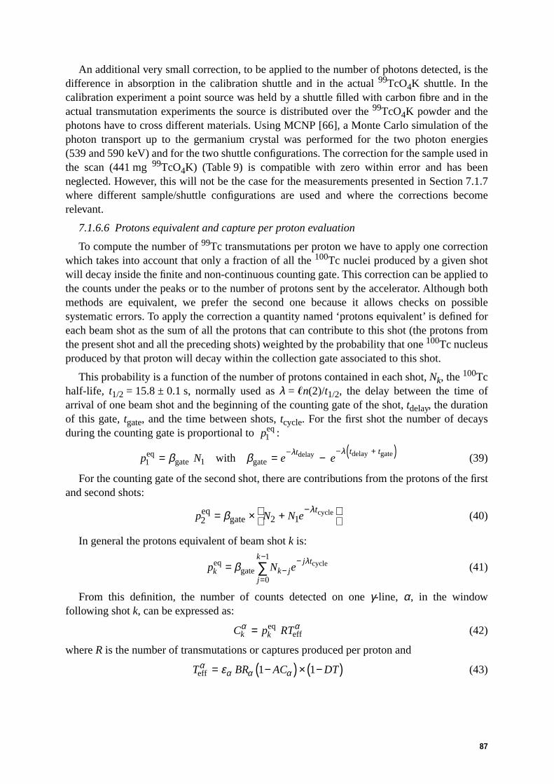
87

An additional very small correction, to be applied to the number of photons detected, is thedifference in absorption in the calibration shuttle and in the actual 99TcO4K shuttle. In thecalibration experiment a point source was held by a shuttle filled with carbon fibre and in theactual transmutation experiments the source is distributed over the 99TcO4K powder and thephotons have to cross different materials. Using MCNP [66], a Monte Carlo simulation of thephoton transport up to the germanium crystal was performed for the two photon energies(539 and 590 keV) and for the two shuttle configurations. The correction for the sample used inthe scan (441 mg 99TcO4K) (Table 9) is compatible with zero within error and has beenneglected. However, this will not be the case for the measurements presented in Section 7.1.7where different sample/shuttle configurations are used and where the corrections becomerelevant.

7.1.6.6 Protons equivalent and capture per proton evaluation

To compute the number of 99Tc transmutations per proton we have to apply one correctionwhich takes into account that only a fraction of all the 100Tc nuclei produced by a given shotwill decay inside the finite and non-continuous counting gate. This correction can be applied tothe counts under the peaks or to the number of protons sent by the accelerator. Although bothmethods are equivalent, we prefer the second one because it allows checks on possiblesystematic errors. To apply the correction a quantity named ‘protons equivalent’ is defined foreach beam shot as the sum of all the protons that can contribute to this shot (the protons fromthe present shot and all the preceding shots) weighted by the probability that one 100Tc nucleusproduced by that proton will decay within the collection gate associated to this shot.

This probability is a function of the number of protons contained in each shot, Nk, the 100Tchalf-life, t1/2 = 15.8 ± 0.1 s, normally used as λ = �n(2)/t1/2, the delay between the time ofarrival of one beam shot and the beginning of the counting gate of the shot, tdelay, the durationof this gate, tgate, and the time between shots, tcycle. For the first shot the number of decaysduring the counting gate is proportional to :

(39)

For the counting gate of the second shot, there are contributions from the protons of the firstand second shots:

(40)

In general the protons equivalent of beam shot k is:

(41)

From this definition, the number of counts detected on one γ-line, α, in the windowfollowing shot k, can be expressed as:

(42)

where R is the number of transmutations or captures produced per proton and

(43)

p1eq

p N e et t t

1 1eq

gate gatewith delay delay gate= = −− − +( )β β λ λ

p N N et

2 2 1eq

gatecycle= × +

−β λ

p N ek k jj

k j teqgate

cycle= −=

− −∑β λ

0

1

C p RTk kα α= eq

eff

T BR AC DTeffα

α α αε= −( ) × −( )1 1

88

with εα the efficiency for detecting line α, BRα the branching ratio of line α, DT the globaldead time of the run, and ACα the angular correlation correction for line α. For a run with mshots, the total number of events collected in line α, is:

(44)

where peq is the total protons equivalent of the run. From these expressions, R can be computedfrom each line as:

(45)

All the time parameters involved in the beam and DAQ cycle are known (and constant forthe selected events) with a precision better than 0.1%, and have no significant contribution tothe uncertainty on the total protons equivalent of the run. The half-life of 100Tc is known tobetter than 1% and has negligible contribution to the error. The main uncertainty is comingfrom the beam intensity measurement of each shot. As explained in Section 2.2, the statisticaluncertainties in the beam intensity measurement are small at the intensities used in the rabbitexperiment, and, when added (weighted sum) to compute the total protons equivalent of therun, the statistical uncertainty is very small. However, the systematic uncertainty from thebeam intensity will not average out and will dominate the final uncertainty on the total protonsequivalent of the run. This uncertainty is estimated as 5% for all the rabbit runs.

7.1.6.7 Data quality tests

Before using data for the evaluation of the 99Tc transmutation rate, every run and everyevent had to pass a set of data quality and systematic effects tests (described in detail inRef. [8]).

These data quality tests include the ratio of the number of 100Tc decays observed by the twoHPGe detectors on a given gamma line, tested for both 539 and 590 keV lines [Fig. 86(a)], theratio of the number of 100Tc decays observed on the two lines 539 and 590 keV by the sameHPGe detector [Fig. 86(b)], and the distribution of the time difference between the beam shotand the detection time for the photons in one of the two main γ-lines, collected in the followingDAQ gate, accumulated for all the shots of one run (Fig. 87).

These data quality tests gave us high confidence in the reliability of the data we used andallowed us to remove obvious technical problems.

Fig. 86: (a) Ratio of the 99Tc capture rates measured by the two HPGe counters on the 590 keV line (allruns); (b) Ratio of the number of 99Tc captures per proton computed from the 539 and 590 keV lines withHPGe1 (all runs).

C C p RT p pkk

m

kk

m

αα α= = =

= =∑ ∑

1 1

eqeff

eq eqwith

RC

p BR AC DT=

−( ) × −( )α

α α αεeq 1 1

0 20 40 60 80 100 120 140 160 180Distance to corrected neutron cascade centre (cm)

0 20 40 60 80 100 120 140 160 180Distance to corrected neutron cascade centre (cm)

HP

Ge1

Rat

io 5

39/5

90

1.05

1.00

0.95

0.900.90

0.95

1.00

1.05

1.10

Rat

io H

PG

e1/H

PG

e2 fo

r th

e 59

0 ke

V li

ne

a) b)

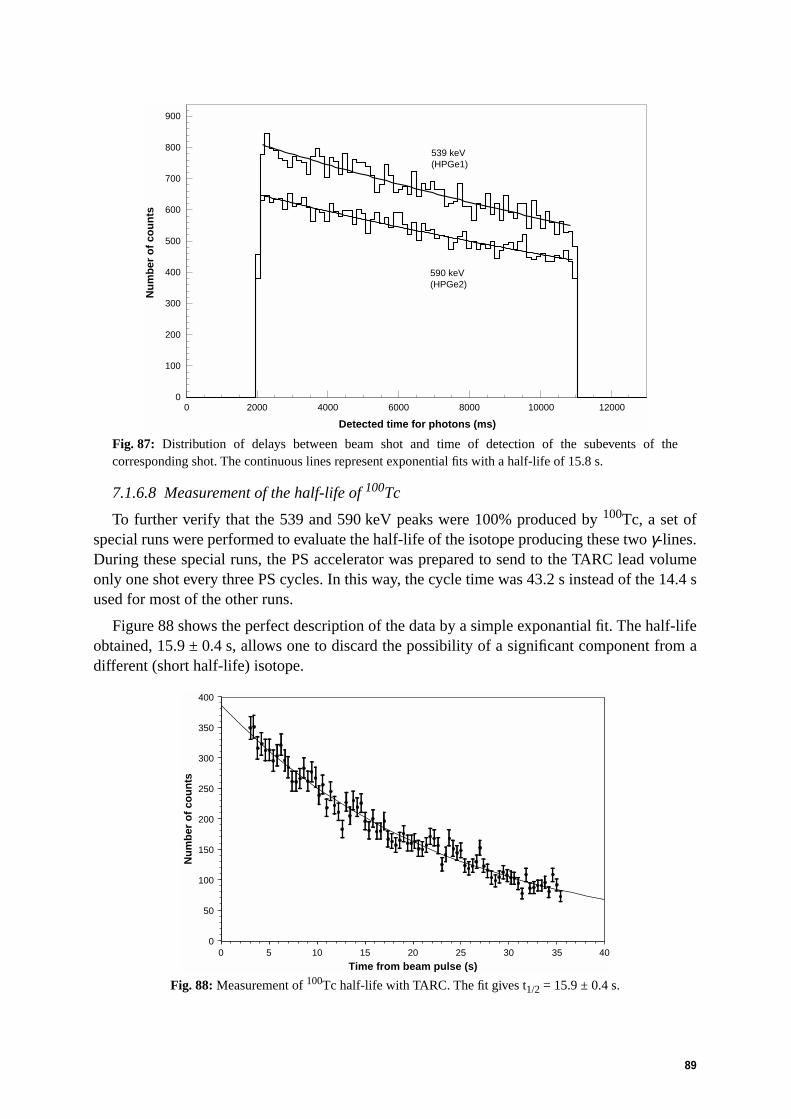
89

Fig. 87: Distribution of delays between beam shot and time of detection of the subevents of thecorresponding shot. The continuous lines represent exponential fits with a half-life of 15.8 s.

7.1.6.8 Measurement of the half-life of 100Tc

To further verify that the 539 and 590 keV peaks were 100% produced by 100Tc, a set ofspecial runs were performed to evaluate the half-life of the isotope producing these two γ-lines.During these special runs, the PS accelerator was prepared to send to the TARC lead volumeonly one shot every three PS cycles. In this way, the cycle time was 43.2 s instead of the 14.4 sused for most of the other runs.

Figure 88 shows the perfect description of the data by a simple exponantial fit. The half-lifeobtained, 15.9 ± 0.4 s, allows one to discard the possibility of a significant component from adifferent (short half-life) isotope.

Fig. 88: Measurement of 100Tc half-life with TARC. The fit gives t1/2 = 15.9 ± 0.4 s.

Detected time for photons (ms)

Nu

mb

er o

f co

un

ts

0

100

200

300

400

500

600

700

800

900

0 2000 4000 6000 8000 10000 12000

539 keV(HPGe1)

590 keV(HPGe2)

0

50

100

150

200

250

300

350

400

0 5 10 15 20 25 30 35 40

Time from beam pulse (s)

Nu

mb

er o

f co

un

ts

90

7.1.6.9 Measured number of captures per proton

An extensive positions scan was performed with the 441.3 mg 99TcO4K sample. For everyrun, the number of counts collected after each selection, on each of the two HPGe counters oneach of the two lines (539 and 590 keV) were evaluated using the weighted average from thethree different methods described in Section 7.1.4.

Table 10: Measured number of captures per proton for different position measurements in the leadvolume. The Error 1 column displays the uncertainties on the average number of captures per protonincluding all statistical and systematic errors except the 14% uncertainty on the γ/β 100Tc branching ratio.The Error 2 column displays the total error on the average. The unit is 10–4 captures per proton and cm forx, y, z.

z (cm) Average (10–4) Error 1 (10–4) Error 2 (10–4)

Hole 1; x = 105; y = 0–7.57.5

67.5112.5

1.251.240.840.39

0.100.100.070.03

0.210.210.140.07

Hole 2; x = 60; y = 3067.5 1.46 0.12 0.25

Hole 3; x = 15; y = 0–112.5–67.5–37.5–22.5–7.57.57.5

22.537.537.567.5

112.5

1.042.263.053.303.433.383.523.102.832.772.040.91

0.080.180.240.260.270.270.280.250.230.220.160.07

0.180.380.520.560.580.570.600.530.480.470.350.15

Hole 4; x = 0; y = –1507.57.5

67.5

0.290.290.20

0.020.020.02

0.050.050.03

Hole 5; x = 0; y = –607.5

67.52.271.48

0.180.12

0.390.25

Hole 6; x = 0; y = 60–112.5–67.5–37.5–22.5–7.57.5

22.537.567.5

112.5

0.801.702.202.272.372.312.182.051.530.68

0.060.140.180.180.190.180.170.170.120.05

0.140.290.370.390.400.390.370.350.260.12

91

The uncertainty was estimated as the sum, in quadrature, of the average uncertainty of thethree evaluations plus the quadratic mean of the deviations to their mean value. From thesenumbers of detected counts, four estimates of the total number of captures are computed perrun (two lines times two detectors), applying the described corrections. The weighted averageof these four estimates is used to compute the number of 99Tc transmutations or captures perincident proton (Table 10).

Figure 89 displays the transmutation rate for holes 3, 6, and 12, respectively, as a functionof the z coordinate. Figure 90 shows the transmutation rate for all the runs in the scan as afunction of the distance to a corrected centre located at x = 0, y = 0, z = –5 cm. The Gaussian fitdemonstrates the high level of spherical symmetry of the distribution. This reflects the similarproperty of the neutron fluence at low energy.

Error 1 in Table 10 includes the statistical error plus the systematic error associated to thedifferent evaluations of the number of counts in the peaks, typically smaller than 2%; theuncertainty on the dead-time correction contributing less than 1% of the total error; theuncertainty on the detector efficiencies, 6%, mainly systematic; the uncertainty on thecorrection for the angular correlation contributing, 1%; and the systematic error on the beam

Hole 7; x = 0; y = 907.5

67.51.551.05

0.130.08

0.260.18

Hole 8; x = 0; y = 1207.5

37.567.5

112.5112.5

0.810.770.600.280.28

0.070.060.050.020.02

0.140.130.100.050.05

Hole 9; x = 0; y = 1507.5

67.50.320.23

0.030.02

0.050.04

Hole 10; x = –45; y = 07.5

67.52.671.73

0.210.14

0.450.29

Hole 11; x = –65; y = 307.5

67.52.101.41

0.170.11

0.360.24

Hole 12; x = –105; y = 0–112.5–67.5–37.5–22.5–22.5–7.57.57.5

22.537.567.5

112.5

0.420.851.081.131.151.171.161.151.101.020.780.37

0.030.070.090.090.090.090.090.090.090.080.060.03

0.070.140.180.190.190.200.200.200.190.170.130.06

z (cm) Average (10–4) Error 1 (10–4) Error 2 (10–4)

92

intensity, 5%. All these components added quadratically result in a value very close to 8% forall the runs in the scan.

Error 2 is the addition in quadrature of error 1 with the 14% common uncertainty in theabsolute branching ratio of 99Tc γ-lines. In Fig. 90 only error 1 is shown.

Fig. 89: Measured number of captures per incident proton in 0.216 g of 99Tc, for three different measuringholes (parallel to the beam line), and for various positions along the holes. Error bars include uncertaintiesfrom statistics, beam intensity (~ 5%), and dead time (~ 0.7%) corresponding to error 1 in Table 10.

Fig. 90: Transmutation rate versus the distance to a corrected centre (x = 0, y = 0, z = –5 cm). The errorbars correspond to error 1 in Table 10. The line is a Gaussian fit.

Hole 3 (X=15,Y=0) cm

Hole 6 (X=0,Y=60) cmHole 12 (X=–105,Y=0) cm

4

3

2

1

0

Cap

ture

s p

er p

roto

n (

216

mg

of

99T

c) (

10–4

)

Position along the beam axis (cm)–150 –100 –50 0 50 100 150

0×100

1×10–4

2×10–4

3×10–4

4×10–4

–200 –150 –100 –50 0 50 100 150 200

Ave

rag

e n

um

ber

of

cap

ture

s p

er p

roto

n

Distance to neutron cascade centre (cm)

σ = 71.6 ± 0.5 cm

93

7.1.7 Monte Carlo simulation and comparison with the data

The EA Monte Carlo [2] adapted for TARC is used in this study [32].

7.1.7.1 Geometry of the irradiation port for the Monte Carlo simulation

Figure 77(b) shows the geometrical description of the rabbit irradiation port used in ourMonte Carlo simulation for the runs with the 441 mg 99TcO4K sample. It includes the precisegeometry and material composition of the irradiation port (steel tubes and lead plugs), theshuttle made of carbon fibre, the polyethylene capsule, the 99TcO4K sample, and obviously thesurrounding lead and hole. Similarly, the different arrangements and material in thecarbon-fibre shuttles, have been simulated for the metallic 99Tc [Fig. 78(a)], the 206 mg99TcO4K [Fig. 78(b)], the aluminium and the silver samples (Fig. 94).

7.1.7.2 Choice of the 99Tc neutron cross-section database

Different databases contain different descriptions of the 99Tc(n,γ) cross-section. TheJENDL nuclear database was used (Fig. 76). However, it must be pointed out that thiscross-section has been evaluated from the analysis of the same experimental data [39] used inmost of the other cross-section databases. A component of the cross-section systematic errorcan be estimated from the spread of the capture rates obtained from the various cross-sectionevaluations all based on the same experimental data (Table 11). The differences reach 10%.

Table 11: The number of captures per proton estimated by Monte Carlo using the different databases forthe 99Tc cross-sections at three positions in the lead volume (441.3 mg 99TcO4K)

The second component of the cross-section systematic error is the uncertainty in theexperimental data used in the evaluation. In the original paper describing those data [39] asystematic error ‘below 10% between a few keV and 10 eV and somewhat above 10% outsidethis energy region’ is quoted.

7.1.7.3 Quality checks of the Monte Carlo simulation

A check is made to determine if the ‘detector’ modifies substantially the neutron flux in itsneighbourhood. The fluxes of neutrons escaping the parallelepipedal surface around thedetector computed with and without the detector are compared. In the case of the rabbitsimulation the difference is found to be of the order of 2% validating the two-step procedurefor the Monte Carlo simulation.

Figure 91 displays the spectra of energies for the neutrons captured by the 99Tc, showingthe fraction of resonant and continuous captures at different positions. As expected, most of thecaptures occur at the two main resonances (5.6 eV and 22.3 eV). For the far position[Fig. 91(b)], the neutron flux is more thermalized leading to a higher fraction of captures at thetwo main resonances.

Database Hole 3, z = +7.5 Hole 6, z = +7.5 Hole 12, z = +7.5

JENDL-3.2 0.401 × 10–3 0.241 × 10–3 0.123 × 10–3

ENDF/B-VI 0.372 × 10–3 0.243 × 10–3 0.120 × 10–3

JEF-2.2 0.379 × 10–3 0.254 × 10–3 0.129 × 10–3

BROND 0.413 × 10–3 0.261 × 10–3 0.130 × 10–3

94

7.1.7.4 Comparison of data and Monte Carlo simulation

The agreement between data and simulation for the full scan of positions is excellent(Fig. 92). The error evaluation includes the experimental data error (Table 10 – ‘Error 1’) andthe Monte Carlo simulation statistical errors. The band around 1 describes the globalsystematic uncertainty in the absolute gamma branching ratio of the 100Tc lines (14%) and10% from the systematic uncertainty of the Monte Carlo prediction.

It must be pointed out that the set of positions (from 15 cm to 170 cm) corresponds to abroadly varying neutron flux, both in magnitude and in energy spectrum. It follows that, amongother features, the Monte Carlo simulation is able to reproduce the varying contributions of thedifferent energy regions of the neutron flux to the 99Tc transmutation, for the differentpositions explored in the lead volume.

Fig. 91: Monte Carlo energy spectra of neutron captures on 99Tc: (a) hole 3, z = +7.5 cm (close to centre);(b) hole 12, z = +67.5 cm (far from centre).

Fig. 92: Comparison of measured and predicted incineration rates in TARC for 99Tc. The grey bandrepresents the overall systematic uncertainty as described in the text.

7.1.8 Systematic studies and other special measurements

In addition to the general scan described in Section 7.1.6, a set of special measurementswith sources different from the 441 mg 99TcO4K, was made to study the possible systematiceffects affecting the results described in Section 7.1.6. The instrumentation hole number 10 at

0

20

40

60

80

100 Hole 3, z = +7.5 cm1 million protons

Nu

mb

er o

f ca

ptu

res

0

100

200

300

400

500

–2 0 2 4 6 8

Hole 12, z = +67.5 cm17.6 million protons

Log10 of neutron energy at capture in 99Tc (eV)–2 0 2 4 6 8

Log10 of neutron energy at capture in 99Tc (eV)

Nu

mb

er o

f ca

ptu

res

a) b)

0.2

0.4

0.6

0.8

1

1.2

0.0 20.0 40.0 60.0 80.0 100.0 120.0 140.0 160.0 180.0

Distance to corrected centre (cm)

Dat

a / M

C

95

z = +7.5 cm was used for these measurements. This position has been selected to have a typicalspallation neutron spectrum, that means not too close to and not too far from the spallationneutron source. The different samples listed below were used: metallic 99Tc (14 mg), 99TcO4Kpowder (0.206 and 0.441 g), natural aluminium (0.883 g), and natural silver (51.839% of107Ag and 48.161% of 109Ag).

The use of different mass, geometry, and chemical form for 99Tc allows one to verify thatthe self-shielding and the self-absorption effects are properly simulated. The capturecross-section of aluminium is relatively well known and the experiment performed allows oneto verify the full procedure used with the rabbit method. For the same reason, natural silver isalso used. Of particular interest is the 109Ag isotope, whose 5.2 eV capture resonance is veryclose in energy to the main resonance, at 5.6 eV, of 99Tc. The study of the incineration rate issimilar to that of 99Tc with the advantages of having no initial radioactivity in the sample and aknown neutron capture cross-section over a large domain of neutron energies and a knownbranching ratio for gamma emission.

7.1.8.1 Self-screening and self-absorption tests

Two extra samples of 99Tc with different masses, chemical compositions, and shapes,already described in Section 7.1.2, were used to compare the rates of transmutation with theresults obtained with the standard sample. These measurements allow one to verify if theself-shielding of the different 99Tc samples is correctly predicted by the Monte Carlosimulation. The different efficiency corrections for self-absorption of photons with respect tothe calibration sources have been taken into account (Table 9).

Figure 93 shows the ratio between the captures per proton per gram for the differentsamples of 99Tc and the value for the metallic sample (14.3 mg 99Tc) as a function of thesample mass. The Monte Carlo prediction confirms that the self-shielding effect is large andshows good agreement with the data. The errors do not include the common 14% from the γ/β100Tc branching ratio.

Fig. 93: Ratio of capture rates per gram of different 99Tc samples to the metallic one. 99Tc masses areindicated in the legend. Both data and Monte Carlo simulation are shown.

Cap

ture

rat

e p

er g

ram

. Sam

ple

/Met

allic

sam

ple

0 50 100 150 200 250Tc mass (mg)

1.2

1

0.8

0.6

0.4

0.2

0

Data_Met/Met

Data<c/p>_101mg/14.3mg

Data<c/p>_216mg/14.3mg

MC<c/p>_101mg/14.3mg

MC<c/p>_216mg/14.3mg

96

7.1.8.2 Cross-check of the rabbit method with silver and aluminium samples

We used a silver sample, whose neutron capture properties are well known and presentsome similarities to those of technetium, to verify the overall procedure for the rabbit system.The silver nucleus has a resonance energy (5.2 eV) close to that of 99Tc (5.6 eV). The sampleis a metallic foil of 50 ± 0.1 mg of pure (99.99%) natural silver with the dimensions shown inFig. 94(a). The sample is held inside the same support used for the metallic 99Tc.

A 880 ± 1 mg pure (99.999%) natural aluminium (27Al) sample has also been irradiated. Itsgeometry and the polyethylene support used to ensure its precise position inside the shuttle areshown in Fig. 94(b).

Fig. 94: Schematics of (a) the Ag sample and (b) the Al sample arrangements inside the shuttle and thepolyethylene holding pieces.

Six gamma peaks characteristic of the de-excitation of 108Ag and 110Ag (443, 614, 633,657, 815 and 1125 keV) [67] are observed in the energy domain between 200 keV and 2 MeV.

The analysis method is similar to that used for 99Tc and is described in detail in Ref. [8].The transmutation rates measured in the instrumentation hole 10 at z = +7.5 cm, after allcorrections have been applied, are summarized in Table 12.

Table 12: Measured and simulated number of captures per proton in hole 10 at z = +7.5 cm for the threeconfigurations of the 99Tc sample, the Ag and Al samples

In total, five samples, three of 99Tc, one of Ag and one of Al were used in the rabbit fortransmutation measurements. Figure 95 shows the transmutation rate ratios, data over MonteCarlo simulation, for the different samples. Within their systematic error of 10% the MonteCarlo simulation results are consistent with the data.

Sample or isotope Measured captures per proton MC captures per proton

441.3 mg 99TcO4K206 mg 99TcO4K14.3 mg metallic Tc25.9 mg 107Ag24 mg 109Ag880 mg 27Al

(2.67 ± 0.21) × 10–4

(1.38 ± 0.11) × 10–4

(3.27 ± 0.25) × 10–5

(2.43 ± 0.16) × 10–5

(1.21 ± 0.11) × 10–5

(5.96 ± 0.35) × 10–6

(3.05 ± 0.11) × 10–4

(1.53 ± 0.02) × 10–4

(3.41 ± 0.10) × 10–5

(2.68 ± 0.09) × 10–5

(1.18 ± 0.02) × 10–5

(6.28 ± 0.42) × 10–6

15 mm

6 mm

6 mm

50 µm

5.5 mm

Ag metallicm = 50 mgd = 10.5 g/cm3

Polyethylene

Al metallicm = 0.88 grd = 2.69 g/cm3

15 mm

15 mm

15 mm

1.01mm

6 mm

3 mm

Polyethylene

3.98 mm

b)

a)

97

Fig. 95: Ratio of the measured number of captures per proton over the Monte Carlo predictions (thedatabase used is JENDL-3.2 except for 27Al for which we used JEF-2.2) in the instrumentation hole 10 atz = +7.5 cm for the various samples used. Data from the two germanium detectors and from the twogamma lines, in the case of 99Tc, are shown separately.

7.1.8.3 Conclusion of rabbit measurements

With the rabbit system, a subset of the TARC experiment, the transmutation of 99Tc basedon the Adiabatic Resonance Crossing method, was studied using the flux of spallation neutronscreated and subsequently diffusing in a large lead volume.

Transmutation of 99Tc has been clearly observed from the photon spectra of thede-excitation of 100Ru* produced by 100Tc decay. These spectra include nine γ-linesidentifying uniquely this isotope. Furthermore, the half-life of the two main lines used tocompute transmutation rates (539 keV and 590 keV) were measured providing additionalconfirmation of the negligible level of background to 100Tc decay. A detailed and extensivestudy of the possible systematic uncertainties contributing to the observed transmutation rateshas also been performed, and the corresponding corrections have been applied.

The 99Tc transmutation rate has been measured in a large number (58) of widely distributedpositions inside the lead volume. Over which the neutron flux varies both in intensity and inenergy. Data coherency is further assured because at each position we made four differentmeasurements (two HPGe detectors and two main γ-lines). This set of data constitutes inaddition an excellent benchmark for any simulation program needed to study transmutationsystems. In particular, it constitutes a precise validation of the simulation developed for theEnergy Amplifier by the CERN EET Group with which our data are very well reproduced.

7.2 129I and 127I integral transmutation rate measurements

The incineration rate of the second most offending LLFF, 129I, has also been measured aspart of our study of the Adiabatic Resonance Crossing method. In this section, we summarizethe procedure used for collecting and analysing the data to measure the neutron capture rate ona sample of iodine containing an isotopic mixture of 86.1% of 129I and 13.9% of 127I. Thesample was obtained in a solid phase as 286.85 ± 1.4 mg of PbI2 (Fig. 96). A more detaileddescription of the sample can be found in Refs. [8] and [68].

0

0.2

0.4

0.6

0.8

1

1.2

1.4

HPGe1(539 keV,Al,Ag)

HPGe2(539 keV,Al,Ag)

HPGe1(590 keV)

HPGe2(590 keV)

99Tc 99Tc 99Tc 27Al 107Ag 109Ag(14 mg) (101 mg) (216 mg) (880 mg) (50 mg nat. Ag)

Dat

a / M

on

te C

arlo

Sample

98

Fig. 96: (a) Configuration of the iodine sample. The material around the iodine sample is a special carbonfibre described in Section 7.1.2.2. (b) Properties of the iodine sample.

7.2.1 Iodine capture and decay schemes

7.2.1.1 Iodine incineration scheme

Through neutron capture, 129I which has a half-life of 1.57 × 107 y is transmuted into twopossible states of 130I with relatively short half-lives (9 min for the isomer and 12.36 h for theground state). Therefore, the corresponding radioactivity disappears rapidly as they botheventually lead to 130Xe which is stable.

The 13.9% of stable 127I, contained in the sample can capture neutrons and produce 128I.We have used the detection of 128I as a technical check of our various procedures (chemistry toprepare the sample and activation procedure).

A simplified decay scheme for 130mI and 130gI is shown in Fig. 97(a) and for 128I inFig. 97(b), where only the levels of interest to this analysis have been kept.

With high-energy neutrons, another possible channel is the (n,2n) reaction on 129Iproducing 128I in principle in competition with (n,γ) reactions on 127I. The threshold is8.8 MeV and our Monte Carlo simulation indicates a totally negligible rate (about 0.04% of theneutron capture rate on 129I at the closest position to the centre of the lead assembly). Thisproduces additional 128I atoms to those produced in the 127I neutron capture, but the addition isat most 0.5%.

The other possible (n,2n) reaction is on 127I with a threshold at 9.1 MeV producing 126I(t1/2 ~ 13.11 d). The rate corresponds to 0.05% of 127I captures and can be neglected. As acheck, we verified that there is no sign of 388.6 keV (Br = 32.2%) and 666.3 keV (Br = 31.3%)γ’s from possible 126I decays in the high statistics Ge counting of activation in hole 3, atz = +7.5 cm.

7.2.1.2 Gamma branching ratios in iodine isotopes

Table 13 gives the values of the branching ratios we used, for the various gamma linesproduced in the decays of the isotopes of interest. In addition, the probability for the 130mI stateto decay to the ground state is taken as P = 84.2% [63] [Fig. 97(a)]. The decay schemes fromRef. [63] have been chosen, since it is the latest compilation available, but also because, as weshall see, it gives a good consistency between the activities obtained from each individualgamma line.

Element Mass and error(mg)

129I127I 10.44 (0.20)

Pb 190.39 (2.10) H2

O2

Total

Density (g/cm3)

y

x

6 m

m

9 mm

Density = 1.13g/cm3

Assembled shuttle with iodine sample

Details of sample configuration

PbI2 +PbOH2O

Carbon Fibre

9.5

15.59.

5.

33.5

6.

a) b)

64.70 (1.00)

1.26 (0.02)20.06 (0.30)286.85 (1.40)1.13 (0.01)

SAMPLE INFORMATION

99

Fig. 97: Simplified decay scheme, derived from Ref. [63], for a) 130mI and 130gI and b) 128I. Insideparentheses, we indicate both the probability to reach the level directly through β-decay and the totalprobability to reach the level.

Table 13: Gamma branching ratios (taken from Ref. [63]) in the various decays of interest

7.2.2 Data analysis

7.2.2.1 Irradiation procedure

We used the PS proton beam, with a momentum of 3.5 GeV/c, extracted directly from thePS in the fast extraction mode (bunch length ~ 20 ns). The number of protons for eachindividual PS shot is measured with beam transformers as already described in Section 1 andin Ref. [14]. The activation data are summarized in Table 14.

a) 130gI decay b) 130mI decay c) 128I decay

130gI lines(keV)

Branchingratio (%)

Error(%)

130mI lines(keV)

Branchingratio (%)

Error(%)

128I lines(keV)

Branchingratio (%)

Error(%)

418.0 34.57 0.1 536.1 15.64(*) 0.1 442.9 12.81(*) 0.1

536.1 98.82 0.1 586.1 1.06(**) 0.01 526.6 1.20(**) 0.01

586.1 1.46 0.01 (*) 16.7% from Ref. [69](**) 1.14% from Ref. [69]

(*) 16.0% from Ref. [69](**) 1.50% from Ref. [69]

668.6 96.2 0.1

739.5 82.58 0.1

1157.5 11.41 0.1

130Xe

(0 %, 98.82%)

130mI

5+

2+9.0 m

12.36 h

39.95 keV

...

(8.6 ps)

39.95 keV

0 keV

β−

0+

(0 %, 1.687%)

(46.7 %,46.7%)

(48 %, 82.583%)

16 % β−

536.085 keV

1122.147 keV

1204.61 keV

1944.09 keV

2362.08 keV (9.4 ps)

100 %

(0.4 %, 96.12%)

(14.0 %, 15.624%)

(1.15 %,1.225 %)

2150.2 keV

(0.51 %, 0.51 %)

130gI

IT 84.2 %

2427.17 keV

(0.184 %,0.184%)

2171.64 keV

(2.14 %,2.14%)

(0.173 %,0.197%)

2081.96 keV (0.022 %,0.035%)

2059.60 keV

1632.53 keV

1808.18 keV

(0 %, 1.268%)

(1.43 %, 2.181%)

2502.23 keV

(0.102 %, 0.102%)

418.

01 k

eV

1157

.47

keV

739.

48 k

eV

668.

54 k

eV

586.

05 k

eV53

6.08

5 ke

V

128Xe

128I 1+24.99 m

7.7×1024 y

0+

93.1 % β−

442.9 keV(23.8 ps)

(1.51 %, 1.5123 %)

128Te

EC 6.9 %

969.475 keV

(11.6 %, 12.807 %)

(80.0 %, 93.1 %)

526.557 keV1.199 %

442.9 keV12.807 %

969.458 keV0.313 %

a) b)

100

Table 14: Summary of activation run information

Assuming that at a given position in the lead assembly, Ni atoms of 130mI (isomer) and Ngatoms of 130gI (ground state) are produced per 109 incident protons, we can calculate thenumber of 130mI and 130gI atoms present at the end of irradiation in the following way.

7.2.2.1.1 Direct production of 130mI

The total number of 130mI atoms present at the end of the irradiation is given by:

(46)

where Xn is the number of protons (in units of 109 protons) in beam shot n,λm = 1.28360 × 10–3 s–1 is the decay constant of 130mI, tend is the time of the last PS shot, andtn is the time of shot number n. Figure 98(a) is an example of the time evolution of thecontribution of each PS shot to the number of 130mI atoms directly produced by neutroncapture and still present at the end of the irradiation.

Fig. 98: a) Quantity versus PS shot number (n). This quantity multiplied by Nirepresents the number of atoms of 130mI produced by shot n and still present at the end of irradiation;b) Quantity versus PS shot number (n). This quantity multiplied by Ng represents thenumber of atoms of 130gI produced by shot n and still present at the end of irradiation.

7.2.2.1.2 Direct production of 130gI

The total number of 130gI atoms present at the end of the irradiation is given by:

(47)

Activation Holez pos. (cm)

Distance to centre (cm)

PS cycle(s)

ShotsNumber of

protons

1

2345678

121036101111333

+67.5+7.5+7.5+7.5+7.5+7.5+7.5+7.5+22.5+22.5

124.8245.6216.7761.8545.6268.7668.7616.7727.0427.04

14.4

14.414.414.414.414.419.219.2

3151791531291391281261263

112

8.507 × 1010

3.702 × 1011

3.028 × 1011

1.297 × 1012

1.638 × 1012

9.997 × 1011

1.576 × 1012

1.219 × 1012

3.276 × 1010

1.060 × 1012

N N X e t t

n

n N( I)m

end i nm end n130

1= × − −( )

=

=∑ λ

0

2

4

6

8

1

1

14

16

a) Activation number 4; Production of 130mI

0

2

4

6

8

10

12

14

16

18b) Activation number 4; Direct Production of 130gI

0 20 40 60 80 100 120 140PS shot number

0 20 40 60 80 100 120 140PS shot number

Ato

ms

130g

I

Ato

ms

130m

I

X e t tn

m end n× − −( )λ

X et t

ng end n× − −( )λ

N N X et t

n

n N( I)g

end g ng end n130

1

= × − −( )=

=∑ λ

101

where λg = 1.55777 × 10–5 s–1 is the decay constant of 130gI. Figure 98(b) shows an exampleof the time evolution of the contribution of each PS shot, to the number of 130gI atoms, directlyproduced by neutron capture and still present at the end of the irradiation.

7.2.2.1.3 Indirect production of 130gI

Since the 130mI isomer has a relatively short half-life and since it decays through internaltransition to the ground state with a probability P = 84.2%, the 130mI isomer produced directlyacts as a source of 130gI atoms. The number of 130gI atoms, present at the end of the irradiationand due to isomer production and decay is given by:

(48)

The numerical value of the factor P × λm/(λg – λm) is – 0.85234. Figure 99(a) illustrates thetime evolution of the contribution of each PS shot to the number of 130gI atoms indirectlyproduced by the decay of 130mI and still present at the end of the irradiation.

Fig. 99: a) Plot of versus PS shot number (n),representing the indirect production of 130gI. This quantity multiplied by Ni represents the number ofatoms of 130gI due to shot n produced by 130mI decay and still present at the end of irradiation; b) Plot ofthe quantity versus PS shot number (n). This quantity multiplied by Nk represents thenumber of atoms of 128I produced by shot n and still present at the end of irradiation.

7.2.2.1.4 Production of 128I

The number of 128I atoms, present at the end of the irradiation is given by:

(49)

where λk = 4.62283 × 10–4 s–1. Figure 99(b) shows an example of the time evolution of thecontribution of each PS shot to the number of 128I atoms produced by neutron capture and stillpresent at the end of the irradiation.

The quantities:

characterize a given irradiation and are calculated for each run (Table 15).

The statistical errors are negligible. The main systematic error comes from the absolutebeam calibration uncertainty (5%).

N P N X e

t te

t t

n

n N( I)m g

end im

g mn

m end n g end n130

1

→ ( ) ( )=

== × ×

−× − − −

− −∑

λλ λ

λ λ[ ]

0

1

2

3

4

5

6

7

8

9

10a) Activation number 4;Indirect 130gI Production

0

2

4

6

8

10

12

14

16

18b) Activation number 4; Production of 128I

0 20 40 60 80 100 120 140

PS shot number0 20 40 60 80 100 120 140

PS shot number

Ato

ms

128 I

Ato

ms

130g

I

P X e et t t t× −( )[ ] × × −

− −( ) − −( )λ λ λ λ λm g m n

m end n g end n/

X e t tn

k end n× − −( )λ

N N X e t t

n

n N( I)end k n

k end n128

1

= × − −( )=

=∑ λ

A N N B N N

C N N D N N

≡ ≡

≡ ≡→

( I) ; ( I) ;

( I) ; ( I)

mend i

gend g

m gend i end k

130 130

130 128

102

Table 15: Beam integrals (A, B, C and D) calculated for each irradiation run. These beam integralscharacterize the production of 130mI, 130gI and 128I during the irradiation. They represent numbers ofprotons in units of 109 protons.

7.2.2.2 Gamma spectra analysis

7.2.2.2.1 Procedure and calibration

The iodine sample was quickly (within 3 min) taken to the CERN/TIS Ge counter system,where the activity of the various gamma lines of interest was measured. Several short countingperiods (600, 600 and 900 seconds) were performed at the beginning to allow us to detect theeffect of the short decay time of 130mI. Then, longer countings were made to detect, with highstatistics, the 130gI at longer times where it dominates the sample activity.

Several calibrations of the Ge counter were made using a 152Eu source and also a 133Basource. The activity of the 152Eu is known to ± 5%.

7.2.2.2.2 Correction for extended source geometry and gamma absorption

The Ge calibration is performed with a naked point-like source, therefore, we need tocalculate corrections to take into account that (a) the iodine sample is an extended source of γ’sand (b) that the γ’s produced can be absorbed in the iodine sample itself as well as in the shuttlematerial. Absorption in the Ge counter material (aluminium window, etc.) is common to thecalibration procedure and to the data taking.

The correction was obtained by a simulation performed using both MCNP [66] and FLUKAcodes [20]. The results are given in Table 16. They are found to be small (≤ 5%).

Table 16: Efficiencies obtained from point-like source calibration, for positions D1 and D2, and relativecorrections to the efficiencies for extended source geometry and absorption obtained with MCNP

Activation A B C D

12345678

107118508612387614403395

39429912791620986155411991076

218153656857509800696579

21620688010906771068763714

Energy (keV)Eff. at D1

(%)Corr. at D1

(%)Eff. at D2

(%)Corr. at D1

(%)

417.93443

526.5536.1586.37668.57739.51156.9

1.251.160.9490.9310.8490.7520.6930.497

4.964.553.533.443.032.522.191.16

0.4010.3770.3150.3090.2830.2510.2300.159

4.474.083.133.052.672.191.890.95

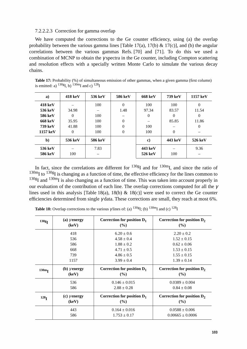
103

7.2.2.2.3 Correction for gamma overlap

We have computed the corrections to the Ge counter efficiency, using (a) the overlapprobability between the various gamma lines [Table 17(a), 17(b) & 17(c)], and (b) the angularcorrelations between the various gammas Refs. [70] and [71]. To do this we used acombination of MCNP to obtain the γ spectra in the Ge counter, including Compton scatteringand resolution effects with a specially written Monte Carlo to simulate the various decaychains.

Table 17: Probability (%) of simultaneous emission of other gammas, when a given gamma (first column)is emitted: a) 130gI, b) 130mI and c) 128I

In fact, since the correlations are different for 130gI and for 130mI, and since the ratio of130mI to 130gI is changing as a function of time, the effective efficiency for the lines common to130gI and 130mI is also changing as a function of time. This was taken into account properly inour evaluation of the contribution of each line. The overlap corrections computed for all the γlines used in this analysis [Table 18(a), 18(b) & 18(c)] were used to correct the Ge counterefficiencies determined from single γ data. These corrections are small, they reach at most 6%.

Table 18: Overlap corrections to the various γ lines of: (a) 130gI; (b) 130mI and (c) 128I

a) 418 keV 536 keV 586 keV 668 keV 739 keV 1157 keV

418 keV536 keV586 keV668 keV739 keV1157 keV

–34.98

035.9541.88

0

100–

100100100100

01.48

–000

10097.34

0–

100100

10083.57

085.85

–0

011.54

011.86

0–

b) 536 keV 586 keV c) 443 keV 526 keV

536 keV586 keV

–100

7.83–

443 keV526 keV

–100

9.36–

130gI(a) γ energy

(keV)Correction for position D1

(%)Correction for position D2

(%)

4185365866687391157

6.20 ± 0.64.58 ± 0.41.88 ± 0.24.71 ± 0.54.86 ± 0.53.99 ± 0.4

2.20 ± 0.21.52 ± 0.150.62 ± 0.061.53 ± 0.151.55 ± 0.151.39 ± 0.14

130mI(b) γ energy

(keV)Correction for position D1

(%)Correction for position D2

(%)

536586

0.146 ± 0.0152.88 ± 0.28

0.0389 ± 0.0040.84 ± 0.08

128I(c) γ energy

(keV)Correction for position D1

(%)Correction for position D2

(%)

443586

0.164 ± 0.0161.753 ± 0.17

0.0588 ± 0.0060.00665 ± 0.0006

104

7.2.2.2.4 Systematics in shuttle positioning

It was possible to monitor the relative position of the shuttle, using the 39.5 keV gammaemitted by 129I with a 7.52% branching ratio. The maximum spread between rates observed forthe 39.5 keV line is 2.6% at D1 and 1.13% at D2, which, when transformed into a spread inposition, gives respectively 0.6 and 0.5 mm displacements expected for D1 = 43 mm andD2 = 93 mm. The absolute position has an error of 1 mm. Therefore, the overall systematicerror in the shuttle position is estimated to be 1.1 mm.

7.2.2.3 Peak analysis

The number of counts in the peaks was determined in three ways: (a) using the standardalgorithm available from the CERN/TIS Ge system (Inter gamma Analysis), which has theadvantage of being very robust; (b) using an algorithm used also for the rabbit analysis [61](see Section 7.1), and (c) making a fit with an interactive software (PAW), in cases ofambiguity of results from (a) and (b). This allowed us to compare the methods, and gave us away to correct problems and estimate the systematic errors. In all cases the γ’s of interest aresufficiently separated from one another (Fig. 100) to have a reasonably good measurement ofthe number of counts.

A practical overall test of the peak fitting performance, the estimation of the Ge counteracceptance, the effect of γ overlap and the determination of the γ-line branching ratio isobtained by verifying that all the γ-lines of one element give the same activity. This is indeedthe case both for 130gI and for 128I γ’s. Furthermore, since for 130gI there are six different γlines, the spread between the activities of these lines, averaged over the eight activations, is agood measure of the systematic error. We find a standard deviation of 4%, which we use in oursystematic error analysis.

Fig. 100: Comparison of first and sixth countings for activation number 7 in hole 3 at z = 7.5 cm, showingthe disappearance of the 128I peaks (443 and 526 keV) after nine half-lives of 128I (the rate of the sixthcounting is multiplied by 10 to avoid overlap of spectra).

7.2.2.4 Calculation of capture rates

We define the origin of time as the end of the irradiation time (time of the last PS shot). Atthat moment we have a certain number of 130mI atoms, n1(0), and a certain number of 130gIatoms, n2(0), which can be expressed as:

1

10

100

100

1000

10000

100000

400 500 600 700 800 900 1000 1100 1200

128I 128I

Photon energy (keV)

Nu

mb

er o

f co

un

ts

Counting # 6

Counting # 1

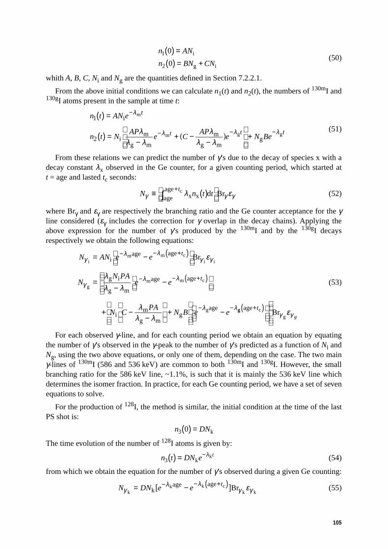
105

(50)

whith A, B, C, Ni and Ng are the quantities defined in Section 7.2.2.1.

From the above initial conditions we can calculate n1(t) and n2(t), the numbers of 130mI and130gI atoms present in the sample at time t:

(51)

From these relations we can predict the number of γ’s due to the decay of species x with adecay constant λx observed in the Ge counter, for a given counting period, which started att = age and lasted tc seconds:

(52)

where Brγ and εγ are respectively the branching ratio and the Ge counter acceptance for the γline considered (εγ includes the correction for γ overlap in the decay chains). Applying theabove expression for the number of γ’s produced by the 130mI and by the 130gI decaysrespectively we obtain the following equations:

(53)

For each observed γ-line, and for each counting period we obtain an equation by equatingthe number of γ’s observed in the γ-peak to the number of γ’s predicted as a function of Ni andNg, using the two above equations, or only one of them, depending on the case. The two mainγ-lines of 130mI (586 and 536 keV) are common to both 130mI and 130gI. However, the smallbranching ratio for the 586 keV line, ~1.1%, is such that it is mainly the 536 keV line whichdetermines the isomer fraction. In practice, for each Ge counting period, we have a set of sevenequations to solve.

For the production of 128I, the method is similar, the initial condition at the time of the lastPS shot is:

The time evolution of the number of 128I atoms is given by:

(54)

from which we obtain the equation for the number of γ’s observed during a given Ge counting:

(55)

n AN

n BN CN1

2

0

0

( ) =

( ) = +i

g i

n t AN e

n t NAP

e CAP

e N Be

t

t t t

1

2

( ) =

( ) =−

+ −−

+

−

− − −

i

im

g m

m

g mg

m

m g g

λ

λ λ λλλ λ

λλ λ

( )

N n t tt

γ γ γλ ε≡ ( )

+∫ x xage

age c d Br

N AN e e

NN PA

e e

N CPA

N B e e

t

t

γλ λ

γ γ

γλ λ

λ λ

ε

λλ λ

λλ λ

im m c

i i

gm m c

g

iage age

g i

g m

age age

im

g mg

age

Br= −

=−

−

+ −−

+

−

− − +( )

− − +( )

− −

gg cg

ageBr

+( )

tgγ γε

n DN3 0( ) = k

n t DN e t3( ) = −

kkλ

N DN e e tγ

λ λγ γε

kk k c

k kkage age Br= −− − +( )[ ]

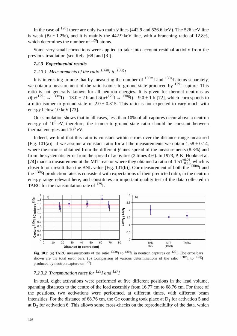
106

In the case of 128I there are only two main γ-lines (442.9 and 526.6 keV). The 526 keV lineis weak (Br ~ 1.2%), and it is mainly the 442.9 keV line, with a branching ratio of 12.8%,which determines the number of 128I atoms.

Some very small corrections were applied to take into account residual activity from theprevious irradiation (see Refs. [68] and [8]).

7.2.3 Experimental results

7.2.3.1 Measurements of the ratio 130mI to 130gI

It is interesting to note that by measuring the number of 130mI and 130gI atoms separately,we obtain a measurement of the ratio isomer to ground state produced by 129I capture. Thisratio is not generally known for all neutron energies. It is given for thermal neutrons asσ(n+129I → 130mI) = 18.0 ± 2 b and σ(n+129I → 130gI) = 9.0 ± 1 b [72], which corresponds toa ratio isomer to ground state of 2.0 ± 0.315. This ratio is not expected to vary much withenergy below 10 keV [73].

Our simulation shows that in all cases, less than 10% of all captures occur above a neutronenergy of 105 eV, therefore, the isomer-to-ground-state ratio should be constant betweenthermal energies and 105 eV.

Indeed, we find that this ratio is constant within errors over the distance range measured[Fig. 101(a)]. If we assume a constant ratio for all the measurements we obtain 1.58 ± 0.14,where the error is obtained from the different γ-lines spread of the measurements (8.3%) andfrom the systematic error from the spread of activities (2 times 4%). In 1973, P. K. Hopke et al.[74] made a measurement at the MIT reactor where they obtained a ratio of which iscloser to our result than the BNL value [Fig. 101(b)]. Our measurement of both the 130mI andthe 130gI production rates is consistent with expectations of their predicted ratio, in the neutronenergy range relevant here, and constitutes an important quality test of the data collected inTARC for the transmutation rate of 129I.

Fig. 101: (a) TARC measurements of the ratio 130mI to 130gI in neutron captures on 129I. The error barsshown are the total error bars. (b) Comparison of various determinations of the ratio 130mI to 130gIproduced by neutron capture on 129I.

7.2.3.2 Transmutation rates for 129I and 127I

In total, eight activations were performed at five different positions in the lead volume,spanning distances to the centre of the lead assembly from 16.77 cm to 68.76 cm. For three ofthe positions, two activations were performed, at different times, with different beamintensities. For the distance of 68.76 cm, the Ge counting took place at D1 for activation 5 andat D2 for activation 6. This allows some cross-checks on the reproducibility of the data, which

1 51 0 160 21. ..

−+

0

0.2

0.4

0.6

0.8

1

1.2

1.4

1.6

1.8

2

0 10 20 30 40 50 60 70 800

0.5

1

1.5

2

2.5

3

BNL325

MIT(1973)

TARC

a) b)

130m

I / 13

0gI

Distance to centre (cm)

Cap

ture

130m

I / C

aptu

res

130g

I

107

is found to be better than 4% in the case of 129I. For each sample activation the number ofneutron captures that occurred on 129I and on 127I is given in Table 19 and Table 20,respectively. The results are also shown in Figs. 105 and 107, for 129I and 127I, respectively.

Table 19: Measured number of captures on 129I, with the corresponding production of 130mI and 130gIatoms, per 109 protons incident on the lead assembly. The errors quoted are peak-finding (stat.) errors only.

Table 20: Measured number of captures on 127I, per 109 protons incident on the lead assembly. The errorsare peak-finding (stat.) errors only.

7.2.4 Comparison with the Monte Carlo simulation

7.2.4.1 Neutron capture cross-section

Both the neutron capture and elastic cross-sections of 129I [Fig. 102(a)] and 127I[Fig. 102(b)] are fairly well known below 2–3 MeV. In the case of TARC we expect to have atleast 90% of neutron captures occurring below a few tens of keV for 129I and below a few keVfor 127I.

The 127I neutron capture cross-section is in principle better known than the 129I one, forwhich the differences between various evaluations result in a difference of up to 12.5%between JENDL-3.2 [5] and the other data bases while it reaches 30% for 129I. Our data favourslightly the JENDL-3.2/JEF-2.2/BROND evaluations [75] of the 129I capture cross-section[Fig. 103(a) & 103(b)].

7.2.4.2 Monte Carlo results

As expected, the distribution of captures reflects the resonance structure in the capturecross-section [Fig. 104(a) & 104(b)] the main one being at 40 eV in the case of 127I and 70 eVin the case of 129I. The capture energy spectrum is significantly harder than in the case of 99Tc,

Activation 130mI 130mI error 130gI 130gI errorTotal 129I captures

Error on total

12345678

1604319652144141606311682108001871118855

596594256236244311556300

10082130647953.4100137454.17644.21355311720

518544226206217277490265

2612532716223682607619136184443226430575

790806341314326416741401

Activation Total 127I capture Error on total

12345678

1442118923135541536811660107841875817922

276309138121134182288154

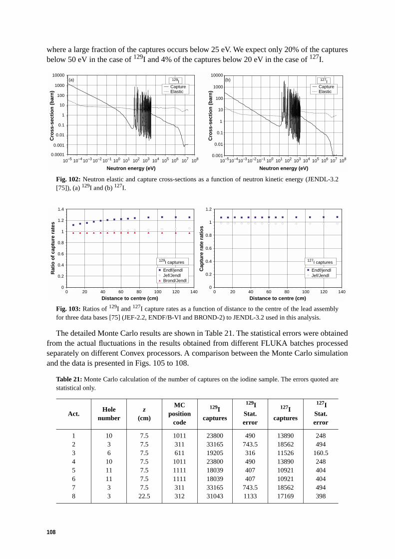
108

where a large fraction of the captures occurs below 25 eV. We expect only 20% of the capturesbelow 50 eV in the case of 129I and 4% of the captures below 20 eV in the case of 127I.

Fig. 102: Neutron elastic and capture cross-sections as a function of neutron kinetic energy (JENDL-3.2[75]), (a) 129I and (b) 127I.

Fig. 103: Ratios of 129I and 127I capture rates as a function of distance to the centre of the lead assemblyfor three data bases [75] (JEF-2.2, ENDF/B-VI and BROND-2) to JENDL-3.2 used in this analysis.

The detailed Monte Carlo results are shown in Table 21. The statistical errors were obtainedfrom the actual fluctuations in the results obtained from different FLUKA batches processedseparately on different Convex processors. A comparison between the Monte Carlo simulationand the data is presented in Figs. 105 to 108.

Table 21: Monte Carlo calculation of the number of captures on the iodine sample. The errors quoted arestatistical only.

Act.Hole

numberz

(cm)

MC position

code

129I captures

129IStat. error

127I captures

127IStat. error

12345678

103610111133

7.57.57.57.57.57.57.522.5

1011311611101111111111311312

2380033165192052380018039180393316531043

490743.5316490407407

743.51133

1389018562115261389010921109211856217169

248494

160.5248404404494398

CaptureElastic

127ICaptureElastic

129I

Cro

ss-s

ecti

on

(b

arn

)

10000

1000

100

10

1

0.1

0.01

0.00110–510–410–310–210–1 100 101 102 103 104 105 106 107 108

Neutron energy (eV)

Cro

ss-s

ecti

on

(b

arn

)

10000

1000

100

10

1

0.1

0.01

0.001

0.000110–5 10–4 10–3 10–2 10–1 100 101 102 103 104 105 106 107 108

Neutron energy (eV)

(a) (b)

0

0.2

0.4

0.6

0.8

1

1.2

1.4

129I captures

0

0.2

0.4

0.6

0.8

1

1.2

127I captures

140120100806040200

Distance to centre (cm)140120100806040200

Distance to centre (cm)

Cap

ture

rat

e ra

tio

s

Endf/jendlJef/JendlBrond/Jendl

Endf/jendlJef/JendlR

atio

of

cap

ture

rat

es

109

Fig. 104: Neutron energy spectra at capture in (a) 129I and (b) 127I samples. The two curves (0311 and1111) correspond to extreme measurement positions (16.77 and 68.76 cm from center of lead volume) inthe lead volume (Monte Carlo codes defining positions are shown in Table 14) and have been normalizedto unit area.

Fig. 105: Comparison of the measured capture rate on 129I with the Monte Carlo simulation based onJENDL-3.2. Error bars include point-to-point errors only (statistics and systematic). For the data there isan additional global systematic error of 8.3%. For the Monte Carlo simulation there is an additional globalsystematic error of 10.8%.

0

0.02

0.04

0.06

0.08

0.1

0.12

0.14

0.16

10–3 10–2 10–1 100 101 102 103 104 105 106 107

03111111

a)

0

0.05

0.1

0.15

0.2

0.25

0.3

0.3503111111

b)

Neutron energy (eV)

10–3 10–2 10–1 100 101 102 103 104 105 106 107

Neutron energy (eV)

Nu

mb

er o

f ca

ptu

res

(arb

itra

ry u

nit

s)N

um

ber

of

cap

ture

s (a

rbit

rary

un

its)

0

5000

10000

15000

20000

25000

30000

35000

0 10 20 30 40 50 60 70 80

129I Monte Carlo129I Data

Distance from centre (cm)

Cap

ture

s o

n 12

9 I p

er 1

09 p

roto

ns

110

Fig. 106: Ratio of measured to predicted (JENDL-3.2) capture rates on 129I as a function of distance fromthe centre of the lead assembly. The error bars include point-to-point systematic errors only. The grey bandshows the global systematic uncertainty.

Fig. 107: Comparison of the measured capture rates on 127I with the Monte Carlo simulation based onJENDL-3.2. Error bars include point-to-point errors only (statistics and systematic). For the data there isan additional global systematic error of 8.4%. For the Monte Carlo simulation there is an additional globalsystematic error of 7.2%.

7.2.5 Systematic errors

The neutron capture measurement error is dominated by the systematic errors. The totalerror in each measurement of the numbers of 129I and 127I captures is 10.5% and 9.9%respectively. A more detailed discussion of systematic errors can be found in Ref. [8].

0

0.2

0.4

0.6

0.8

1

1.2

0 10 20 30 40 50 60 70 80

Captures on 129-I

Distance to centre (cm)

Dat

a / M

on

te C

arlo

0

2000

4000

6000

8000

10000

12000

14000

16000

18000

20000

0 10 20 30 40 50 60 70 80

127-I Monte Carlo

127-I Data

Distance to centre (cm)

Cap

ture

s o

n 12

7 I p

er 1

09 p

roto

ns

111

Fig. 108: Ratio of measured to predicted capture rates on 127I as a function of distance from the centre ofthe lead assembly. The error bars include point-to-point systematic errors only. The grey band shows theglobal systematic uncertainty.

7.2.6 Conclusion

We have measured at five different positions in the TARC lead assembly the neutron capturerates on a sample containing both 129I and 127I. We find an excellent agreement between oursimulation and the TARC measurements.

This iodine measurement is also an integral part of a validation of the Energy Amplifiersimulation, concerning the phenomenology of neutrons in pure lead and the properties offissions fragments. It is shown here that we are able to simulate the neutron capture history of avery small sample (64.7 mg for 129I and 10.4 mg for 127I) placed inside a large assembly of334 t of pure lead.

We have also obtained a new measurement of the production ratio of 130mI to 130gI in 129Icapture, for neutron energies ≤ 105 eV.

7.3 Conclusion on transmutation of long-lived fission fragments

We have measured at a large number of positions inside the TARC lead volume the integralabsolute transmutation rates of 99Tc, 129I and 127I summarized in [Fig. 109(a) & 109(b)].

With the CeF3 crystal used to calibrate the energy–time relation, we also obtainedmeasurements of the 99Tc differential transmutation rate as a function of neutron energy(Fig. 110).

In all cases, the observed transmutation rates (99Tc, 129I and 127I) agree well with theprediction and follow very closely the decrease of neutron fluence as a function of increasingdistances from the centre of the lead volume. This implies that neutron capture at low energiesdominates and that the capture rate per unit of fluence varies little within most of the leadvolume.

0

0.2

0.4

0.6

0.8

1

1.2

0 10 20 30 40 50 60 70 80

Captures on 127-I

Distance to centre (cm)

Dat

a / M

on

te C

arlo

112

The excellent agreement between our simulation and the entire TARC data set validatesfurther our simulation. In turn, the correct prediction of integral and differential transmutationrates for 99Tc and 129I validates the efficiency of the TARC method to transmute LLFFs.

In the case of 99Tc we have obtained a complete set of measurements of all the parametersinvolved in the ARC process: (a) the integral neutron capture rate with the rabbit system; (b)the differential neutron capture rate as a function of neutron energy below 1 keV with the CeF3detector; (c) the neutron capture cross-section below 1 keV. All of this was done in awell-controlled neutron flux which had also been measured precisely using several redundantmethods. We can conclude that these transmutation measurements in TARC complete thedemonstration of the efficiency of the Adiabatic Resonance Crossing effect to be used for thedestruction of the most offending long-lived fission fragments produced in nuclear fission.

Fig. 109: (a) Measurement of transmutation rates for 99Tc (216.11 mg), 129I (64.7 mg) and 127I (10.44 mg)samples as a function of distance from the centre of the lead volume. The lines are Gaussian fits to the data;(b) Ratio between data and prediction for the transmutation rates shown in part (a).

104

105

Nu

mb

er o

f ca

ptu

res

per

109

pro

ton

s

0

0.2

0.4

0.6

0.8

1

1.2

1.4

—200 —150 —100 —50 0 50 100 150 200

99Tc (216.1 mg) 129I (64.7 mg) 127I (10.44 mg)

Distance to the centre of the lead volume (cm)

—200 —150 —100 —50 0 50 100 150 200

Distance to the centre of the lead volume (cm)

Dat

a/M

C

a)

b)

99Tc (216.1 mg)

129I (64.7 mg)

127I (10.44 mg)

113

Fig. 110: Measured transmutation rate (hole 10, z = +7.5 cm) for a 85 mg 99Tc sample as a function ofneutron energy compared to simulation (right-hand scale). Measurement of the 99Tc apparent neutroncapture cross-section as a function of neutron energy, and comparison with the previous measurement byChou et al. [39] extrapolated to zero thickness (left-hand scale).

8 Other Integral Measurements

8.1 Production rates of 233U and 239Pu

We have measured the production rates of 233U from 232Th and of 239Pu from 238U with theuse of delayed γ spectroscopy. Two sets of metallic foils of 232Th and 238U were irradiatedduring the same run inside the lead assembly [76].

8.1.1 Production rate of 233U

In a low-intensity neutron flux the transmutation of 232Th to 233U proceeds through thefollowing nuclear reactions:

In order to measure the production rate of 233U, we detected the gammas of 233U* insteadof those from the de-excitation of 233Pa, since the half-life of 233Pa (27 d) is larger than thehalf-life of 233Th (22.3 min), thus resulting in smaller errors in time measurements, transportof the sample, and gamma counting.

The thorium samples have 99.85% purity, 88.9 µm thickness, 12.7 mm diameter and anaverage weight of 132 mg [48]. The foils were activated during run 767 which lasted 8.5 hoursfor a total of (2.141 ± 0.107) × 1013 protons [15], [16]. The 311.98 keV (38.63%) gamma lineis the most direct gamma emitted from the 233U excited states [59] and has a total attenuationcoefficient of 0.11 cm2/g, which results in the absorption of 1.1% of the γ’s. The samples weremeasured with a GeLi counter and analysed with the help of the Inter Technique GammaSpectrum analysis program. We have used the same calibration of the GeLi detector as thatused in triple-foil activation measurements. The activity of the samples was further normalizedto 109 protons.

1 10 100 1000

Neutron energy (eV)

10—1

100

101

102

103

Ap

par

ent

cro

ss-s

ecti

on

(b

arn

)

105

104

103

E×d

Nca

pt

/ dE

per

109

pro

ton

s106

CaptureCross-section

TransmutationRate

Scale

Scale

TARC Cross Section DataChou et al. Cross SectionTARC Measured 99Tc Capture Rate99Tc Capture Rate Simulation (JENDL-3.2)

232 233 22 3 233 27 233Th Th Pa Un d( ) ( . ) ( ), minγ β β → → →

− −

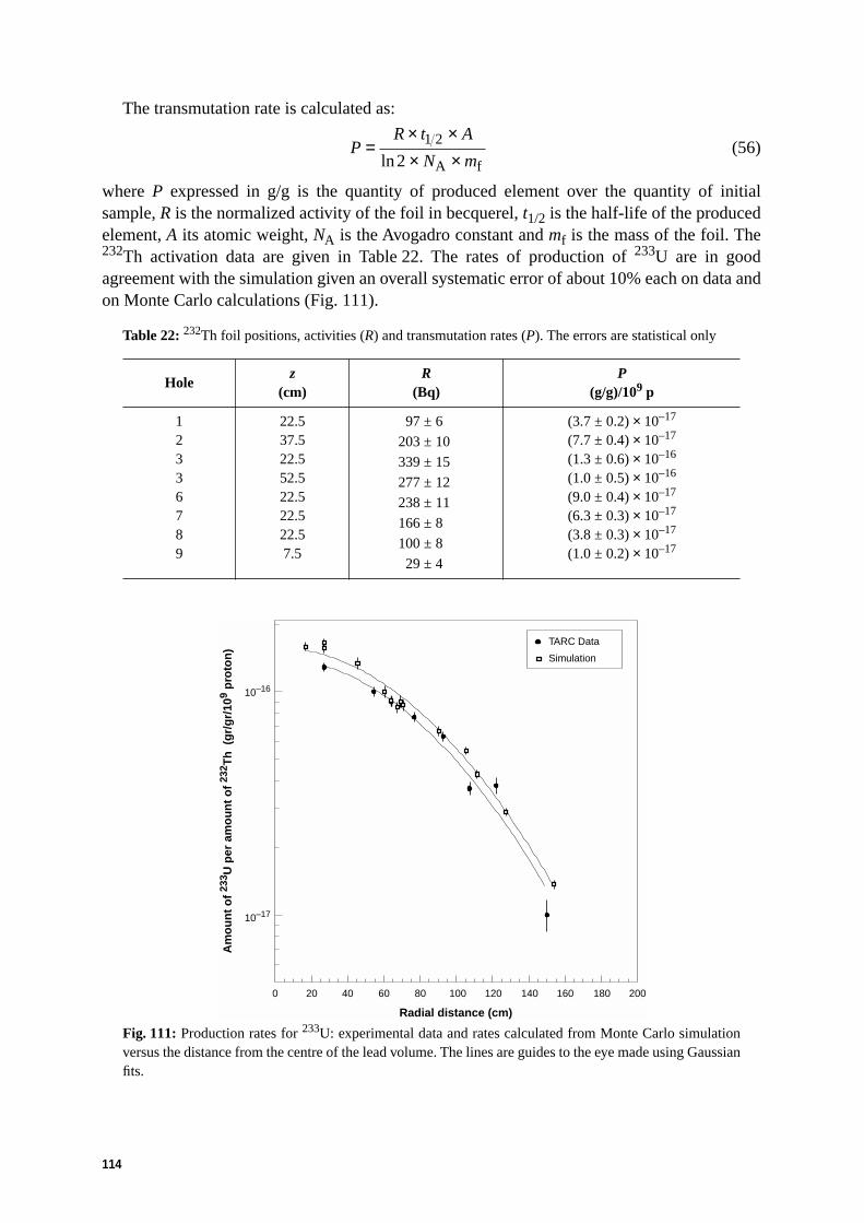
114

The transmutation rate is calculated as:

(56)

where P expressed in g/g is the quantity of produced element over the quantity of initialsample, R is the normalized activity of the foil in becquerel, t1/2 is the half-life of the producedelement, A its atomic weight, NA is the Avogadro constant and mf is the mass of the foil. The232Th activation data are given in Table 22. The rates of production of 233U are in goodagreement with the simulation given an overall systematic error of about 10% each on data andon Monte Carlo calculations (Fig. 111).

Table 22: 232Th foil positions, activities (R) and transmutation rates (P). The errors are statistical only

Fig. 111: Production rates for 233U: experimental data and rates calculated from Monte Carlo simulationversus the distance from the centre of the lead volume. The lines are guides to the eye made using Gaussianfits.

Holez

(cm)R

(Bq)P

(g/g)/109 p

12336789

22.537.522.552.522.522.522.57.5

97 ± 6

203 ± 10

339 ± 15

277 ± 12

238 ± 11

166 ± 8

100 ± 8

29 ± 4

(3.7 ± 0.2) × 10–17

(7.7 ± 0.4) × 10–17

(1.3 ± 0.6) × 10–16

(1.0 ± 0.5) × 10–16

(9.0 ± 0.4) × 10–17

(6.3 ± 0.3) × 10–17

(3.8 ± 0.3) × 10–17

(1.0 ± 0.2) × 10–17

PR t A

N m=

× ×× ×

1 2

2ln A f

Radial distance (cm)

Am

ou

nt

of

233 U

per

am

ou

nt

of

232 T

h (

gr/

gr/

109

pro

ton

)

10–17

10–16

0 20 40 60 80 100 120 140 160 180 200

TARC Data

Simulation

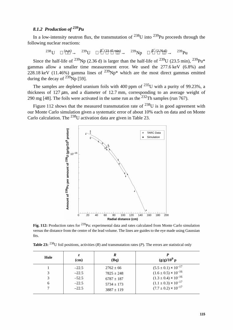
115

8.1.2 Production of 239Pu

In a low-intensity neutron flux, the transmutation of 238U into 239Pu proceeds through thefollowing nuclear reactions:

Since the half-life of 239Np (2.36 d) is larger than the half-life of 239U (23.5 min), 239Pu*gammas allow a smaller time measurement error. We used the 277.6 keV (6.8%) and228.18 keV (11.46%) gamma lines of 239Np* which are the most direct gammas emittedduring the decay of 239Np [59].

The samples are depleted uranium foils with 400 ppm of 235U with a purity of 99.23%, athickness of 127 µm, and a diameter of 12.7 mm, corresponding to an average weight of290 mg [48]. The foils were activated in the same run as the 232Th samples (run 767).

Figure 112 shows that the measured transmutation rate of 238U is in good agreement withour Monte Carlo simulation given a systematic error of about 10% each on data and on MonteCarlo calculation. The 238U activation data are given in Table 23.

Fig. 112: Production rates for 239Pu: experimental data and rates calculated from Monte Carlo simulationversus the distance from the centre of the lead volume. The lines are guides to the eye made using Gaussianfits.

Table 23: 238U foil positions, activities (R) and transmutation rates (P). The errors are statistical only

Holez

(cm)R

(Bq)P

(g/g)/109 p

13367

–22.5–22.5–52.5–22.5–22.5

2762 ± 66

7825 ± 248

6787 ± 187

5734 ± 173

3887 ± 119

(5.5 ± 0.1) × 10–17

(1.6 ± 0.5) × 10–16

(1.3 ± 0.4) × 10–16

(1.1 ± 0.3) × 10–17

(7.7 ± 0.2) × 10–17

238 239 23 45 239 2 36 239U U Np Pun d( , ) ( . min) ( . )γ β β → → → − −

Am

ou

nt

of

239 P

u p

er a

mo

un

t o

f 23

8 U (

gr/

gr/

109

pro

ton

)

10–16

Radial distance (cm)0 20 40 60 80 100 120 140 160 180 200

TARC Data

Simulation

116

8.1.3 Systematic errors

We estimate that the uncertainty in the foil position inside the lead hole is less than 1 cm,which results in less than 1% error in the estimation of the transmutation rate.

The uncertainty on the measured activity R is 7% [5% from absolute activity of calibrationsources, 3% for the efficiency at the γ energy, 3% for the estimation of the γ peak area, 2% forthe positioning precision (±1 mm at 100 mm) and 0.3% to 0.9% for γ branching ratios, the timemeasurement error (2 min) has negligible effect]. The uncertainty on the beam intensity is 5%.

The errors on the physical properties of the sample are negligible. Thus the total systematicerror on the transmutation rates is estimated to be 9% both for 233U and 239Pu.

The systematic error on the Monte Carlo prediction is dominated by the uncertainty on the(n,γ) cross-sections which is hard to estimate. We think that in the case of 232Th(n,γ) it is atleast 10% and, according to the BNL tables [27], it is at least 7% for 238U(n,γ).

Both for 233U and 239Pu production rates measured with a precision of 9%, the results areconsistent with the Monte Carlo simulation obtained with an uncertainty of order 10%.

8.1.4 Protactinium (233Pa) half-life

We checked that the 312 keV γ line used in the previous analysis was due entirely to 233Paby checking its half-life. The activation of 0.25 g of 232Th in hole 5 at z = +7.5 cm was used forour measurement (runs 1303 to 1325). The detailed experimental conditions are described inRef. [77]. The evaluation of the number of counts in the 312 keV peak was made with the samemethods used in the 99Tc and 129I studies [77].

The number of counts in the γ peak can be written as:

(57)

where is the number of captures on 232Th per proton, λ1 = 5.18047 × 10–4 s–1 (233Th);λ2 = 2.97131 × 10–7 s–1 (233Pa); tc is the counting time and age is the time between the lastproton shot and the beginning of a given Ge detector counting period, εγ and Brγ (36.8%) arerespectively the efficiency and the branching ratio of the 312 keV γ-line, α1 and α2 areconstants depending on the beam intensity.

The ratio between two Ge measurements will eliminate the common constants, Eq. (58),( is here the same for all countings):

(58)

This relation is only dependent on measurements from the Ge detector and not on theirradiation. From each equation (58) a value of λ2 was extracted.

The spread in the values of λ2 gives us a check of the consistency of our data. Figure 113shows the results for all calculated λ2 values in the two different positions D1 and D2, λ2 of0.31 × 10–6 ± 0.91 × 10–8 s–1 for position D1, and 0.29 × 10–6 ± 0.51 × 10–8 s–1 for positionD2. The average value for λ2 is introduced in the following expression as a small correction tothe number of γ counts:

(59)

N e e Ntγ

λ λγ γα α ε≅ + −− −( ) ( )1 2

2 21agecThc Br

NcTh

NcTh

N

Ne

e

e

t

tγ

γ

λ λ

λi

j

i jci

cj

(age age )= × −

−

− − −

−2

2

2

1

1

N

eAe

tγλ

λ

1 2−=−

−c

age

117

with

Exponential fits to the data using Eq. (59) allow us to obtain our best estimate of the of233Pa half-life: 27.46 ± 1.8 days which is consistent with the accepted world value of26.96 ± 0.002 days.

No attempt was made to perform a high-precision determination of 233Pa half-life, however,this study is part of a check of the quality of the TARC data.

Fig. 113: Distribution of λ values for the two different positions D1 and D2 and for the three methods ofpeak evolution.

8.2 The 232Th(n,2n)231Th reaction rate

8.2.1 Motivation

In the Energy Amplifier project, the contribution to the neutron multiplication from thenon-fission reactions is not negligible in particular for the proposed fuel which is 232Th.Furthermore, the reactions 232Th(n,2n)231Th → β– + 231Pa and 231Pa(n,γ)232Pa → β– + 232Uleading to the production of 232U which is responsible for a large part of the short-term (fewcenturies) radiotoxicity, while 231Pa is responsible for the long term radiotoxicity, are of greatrelevance. We have exploited the opportunity offered by the TARC experiment to measure the(n,2n) reaction rate of 232Th in a lead slowing downspectrometer environment.

The 232Th(n,2n) reaction has been studied in different laboratories [78], but as far as weknow, has not been measured with spallation neutrons in lead. The measurement is based onthe observation of the gamma rays emitted by 231Th formed by the n,2n reaction on 232Th. Asis well known, natural 232Th is an alpha emitter with many gamma rays emitted during thisde-excitation. The gamma rays from 231Th are superimposed on the natural gamma-raybackground of 232Th. The intensity of the gamma rays from 231Th is extracted from thesubtraction of this background. This introduces a sizeable uncertainty for the determination ofthe n,2n reaction rate.

A N≈ +( ) BrcThα α εγ γ1 2

0

0.5

1

1.5

2

2.5

3

a)

0

2

4

6

8

10

12

14

0 0.1 0.2 0.3 0.4 0.5 0.6

λ2 values for position D2 multiplied by 1060 0.1 0.2 0.3 0.4 0.5 0.6

λ2 values for position D1 multiplied by 106

Mean = 0.2901E–06RMS = 0.3040E–07

Mean = 0.3063E–06RMS = 0.1360E–07

b)

σn, n n n n nd MeV2 6n( ) ( ) ,E E E E∫ ≥( )Φ

118

A special experimental set-up was arranged to observe the 25.6 keV gamma-ray transitionof 231Th. This line has the advantage of a relatively high intensity (14.5%), and lies in thegamma-ray region where the contamination is unlikely. The details of this analysis are given inRefs. [8] and [79]. Here we summarized the main elements of the measurement.

The n,2n energy threshold for 232Th is 6 MeV and the evaluated cross-section is of the orderof 3 barn in the neutron energy range between 6 MeV and 14 MeV. The two samples used(Table 24) have been placed in hole 3 at z = + 7.5 cm and z = 0.0 cm near the centre of the leadvolume in order to maximize the component of the spallation neutrons having an energy above6 MeV.

Table 24: Characteristics of the 232Th samples, irradiation positions in the lead volume, and characteristicsof the proton beam

8.2.2 Photon spectra

The 25.6 keV line can be seen without any ambiguity (Fig. 114), while Fig. 115 showsother peaks of 231Th such as 84.2 keV which are common to 232Th hence harder to separate.Note also the presence of lines at 94.6 and 98.6 keV characteristic of uranium X-rays andprobably originating from other high-energy neutron reactions on 232Th.

We have checked that the half-life of the 25.6 keV line was consistent with the 25.52 hexpected for 231Th [80].

Fig. 114: Observed photon energy distribution from the irradiated and non-irradiated 232Th sample in theenergy range 21–39 keV.

232Thsample

Weight(g)

DimensionThickness

(µm)

Proton kinetic energy(GeV)

Irradiation position

Number ofprotons (1012)

Sample 1 0.158 φ = 1.25 cm 110.3 2.75 (Hole 3, z = 0.0 cm)

4.80

Sample 2 0.678 3 cm × 2.9 cm 66.5 2.75 (Hole 3, z = +7.5 cm)

9.01

0.03

0.04

0.05

0.06

0.07

0.08

0.09

0.1

21 26 31 36

231Th (25.6 keV)

Energy (keV)

Co

un

ts/2

8 eV

/s

Irradiated

Non-irradiated

119

Fig. 115: Observed photon energy distribution from the irradiated and non-irradiated 232Th sample in theenergy range 80–115 keV.

Various sources of background contributing to the γ counting obtained with ahigh-resolution X-ray detector have been studied. Background from the 232Th sample wassubtracted from measurements performed before irradiation. The background from 233Th wasmade negligible by waiting about 10 half-lives (~ 4 h) before counting the 231Th γ’s. Thebackground from bremsstrahlung of β’s from 231Th and 233Pa was made negligible by using aberyllium filter 250 µm thick.

Other potential backgrounds such as fissions of 232Th and 232U, γ’s from 233Pa and from233U were found not to contribute substantially to the 25.6 keV line of interest. Our results forthe two irradiations performed are given in Table 25.

For comparison, the results obtained from the 84.2 keV gamma line are also reported inFig. 116, Fig. 117, and in Table 25. The observed difference between the data (Table 25) isqualitatively consistent with what is expected from the effect of the neutron flux at z = 0.0(close to the centre of the spallation source) being greater than the one at z = +7.5 cm.However, as mentioned above, the 84.2 keV line is not pure and the method used gives asignificant uncertainty in the determination of the counts resulting from the de-excitation of the231Th.

Table 25: Measured reaction rates of 232Th(n,2n)231Th per incident proton and per gram of 232Th usingthe 25.6 and 84.2 keV lines, for each of the samples indicated (hole 3)

The neutron self-shielding was found negligible in the neutron energy range from 6 MeV to14 MeV.

The systematic error on the measurement was not evaluated with precision. We can,however, conservatively state that they are smaller than 50%.

232Th sample z position 25.6 keV line 84.2 keV line

0.678 g0.158 g

7. 5 cm0.0 cm

(1.32 ± 0.13) × 10–6

(6.35 ± 0.63) × 10–7(2.11 ± 0.32) × 10–6

(1.05 ± 0.16) × 10–6

0

0.1

0.2

0.3

0.4

0.5

0.6

0.7

0.8

80 85 90 95 100 105 110 115

Irradiated

Non-irradiated

UKα

232Th + 231Th

Energy (keV)

Co

un

ts/2

8 eV

/s

120

Fig. 116: 232Th(n,2n)231Th reaction rates obtained from the intensities of the 25.6 keV and 84.2 keV lines,from the 3 cm × 3 cm 232Th sample (0.678 g) irradiated in hole number 3 at z = +7.5 cm.

Fig. 117: 232Th(n,2n)231Th reaction rates obtained from the intensities of the 25.6 keV and 84.2 keV lines,from the 0.158 g of 232Th sample irradiated in hole number 3 at z = 0.0 cm.

9 Medical Applications of ARC

9.1 General strategy for medical applications of ARC

9.1.1 Introduction

The domain of applications of the ARC method of enhancement of neutron captures is veryvast. We will discuss in this section the production of (short-lived) isotopes for medicalapplications. Radionuclides are extensively used for medical diagnosis applications as‘tracing’ elements, i.e. they are directly detectable within the patient under study because oftheir spontaneous radioactive decays. In order to minimize the integrated radiotoxicity, thehalf-life of the chosen tracing isotope should be short, ideally not much longer than theexamination time. As a consequence, its utilization is limited to a period of a few half-livesfrom activation, since the radioactivity of the isotope decays exponentially from the moment ofproduction. Another application of growing interest for radionuclides is (cancer) therapy, forwhich doses significantly larger than those used in diagnostics are required. Most of these

0.00

5.0×10–7

1.0×10–6

1.5×10–6

2.0×10–6

2.5×10–6

3.0×10–6

3.5×10–6

4.0×10–6

0 1 2 3 4 5 6

(n,2n)/p 25.6 keV

(n,2n)/p 84.2 keV

Counting number

(n,2

n)

reac

tio

ns/

pro

ton

0.0

2.0×10–7

4.0×107

6.0×10–7

8.0×10–7

1.0×10–6

1.2×10–6

1.4×10–6

1.6×10–6

0 1 2 3 4 5 6 7

(n,2n)/proton 25.6 keV

(n,2n)/proton 84.2 keV

Counting number

(n,2

n)

reac

tio

n r

ate/

pro

ton

121

isotopes must have a relatively short half-life, since they are generally injected or implanted inthe patient’s body. Today the main sources of supply for these isotopes are nuclear reactors orparticle accelerators irradiating a suitable target with a charged-particle beam.

The simplicity of the device (activator) which was proposed by one of us [4] and itsrelatively modest cost and dimensions are intended to promote ‘local’ production of short-livedradioisotopes, thus eliminating costly, swift transportation and the consequent need of largerinitial inventories and thus extending their practical utilization. This is made possible by thehigh neutron capture efficiency resulting from the ARC method, which allows the requiredamount of the radioisotope to be produced with a relatively modest neutron generator.

This method of neutron activation is intended to be a competitive alternative toreactor-driven, neutron capture activation. In addition, several isotopes that are difficult toproduce by activation in the (usually thermal) neutron flux of an ordinary reactor can beproduced using the broad energy spectrum of the neutrons in the activator extending to highenergies and especially designed to make use of the large values of the cross-section at theenergy of resonances. This is the case, for instance, in the production of 99mTc (99Mo), widelyused in medicine and which is nowadays generally chemically extracted from the fissionfragments of spent nuclear fuel. With the present method, this popular radioisotope can beobtained instead by direct neutron resonant activation of a (natural) molybdenum target withthe help of a much simpler and less costly activator driven by a small particle accelerator.Incidentally, the total amount of additional, useless radioactive substances that have to beproduced and handled in association with a given amount of this wanted radionuclide is alsogreatly reduced.

9.1.2 Selected examples of procedures for an activator

The procedures to be followed in order to prepare radioactive samples are illustrated by thefollowing practical examples:

(1) A first procedure, suitable for medical examinations (thyroid), consists of activatingdirectly inside our device an already prepared, pharmacological iodine compound. Theelement is initially available in the most appropriate chemical compound7, made fromnatural iodine (stable isotope 127I). Shortly before administration, the compound isintroduced in the activator driven by a small proton accelerator (23 MeV and 1 mA) andactivated — for instance during a time of the order of one 128I half-life (25 min) orcorrespondingly less for smaller activation strengths — with the help of the capturereaction 127I + n → 128I + γ, which transforms natural iodine into the tracing element128I with β–-decay and a prominent γ-line at 443 keV. There is no chemical ‘preparation’between activation and examination. This very simple procedure is becoming practicalwith the ARC method because of the higher efficiency of neutron capture, whichproduces the required source strength (≤ 1 GBq) starting from a tiny, initial amount ofnatural iodine (≤ 1 g) and using a conventional accelerator of a scale already in wide usewithin hospitals for other applications (PET, etc.). The feasibility of the production of128I from 127I has been confirmed by TARC, using the 127I content of the iodine sampleused in the transmutation test of 129I. The rate of captures measured in TARC is wellreproduced by our simulation (Fig. 118). At about 46 cm from the centre of the leadvolume (hole 10, z = +7.5 cm) the capture rate is 14 900 per 109 protons on our

7. For instance sodium iodide (NaI).

122

10.44 mg sample of 127I. These measurements validate the simulation used in thissection. Our method makes practical the use of 128I as a tracing element for thyroiddiagnosis with a much shorter half-life (25 min) than the one of currently used iodineisotopes (131I and 123I) and hence the corresponding important advantage of a muchsmaller dose to patients8.

Fig. 118: Ratio of measured to simulated capture rate on our 10.44 mg 127I sample. The grey bandrepresents the size of the common systematic error.

(2) A second example, also tested in TARC (see Section 9.2), illustrates the case in whichsome (simple) chemical transformation is needed between the activation and the use ofthe radioactive compound. This is the case for the 99mTc medical examination, of whichmany millions are performed annually world-wide. The small sample to be irradiatedconsists of molybdenum9, for instance in the form of MoO3. The appropriate sample of99Mo (t1/2 = 65 h) is produced with the help of the activator driven by an accelerator andthe capture reaction 98Mo + n → 99Mo + γ. The activated molybdenum sample is thenhandled according to a generally used procedure: transformed for instance in the form ofan appropriate salt, it is captured in an alumina absorber. The production of 99mTcproceeds inside the absorber through the subsequent β-decay reaction 99Mo → 99mTc.The 99mTc which has a relatively short half-life (t1/2 = 6.01 h) is extracted in the form ofTc4+, for instance by passing a solution of water with a small amount of NaCl throughthe Mo sample in the alumina (which remains insoluble). Since only a very smallfraction of the compound is activated at each exposure, the molybdenum ‘father’ can be

8. The current methods of iodine examinations are based on 131I, which has a relatively long half-life of eightdays and which causes large intake doses for the patients (roughly in the ratio of half-lives (461/1), and123I which has the shorter half-life of 13.2 hours (31.8 times that of 128I), but is difficult and costly toobtain since it is normally produced by 30 MeV protons with the (p,2n) reaction on isotopically separated124Te (natural abundance 4.79%). In order to use natural Xe, the reaction is (p,5n) and the energy must beat least 60 MeV. The presently proposed method has therefore both a very simple application and leads tomuch smaller doses to the patient for a given disintegration rate during the examination. We note that thelarger doses of the current methods generally hamper extensive application in the case of young subjectsand of pregnant women.

9. The isotopic content of 98Mo in natural molybdenum is 24.13%. Isotopic enrichment will be convenient,though not mandatory.

0

0.2

0.4

0.6

0.8

1

1.2

0 10 20 30 40 50 60 70 80

Captures on 127-I

Distance to centre (cm)

Dat

a / M

on

te C

arlo

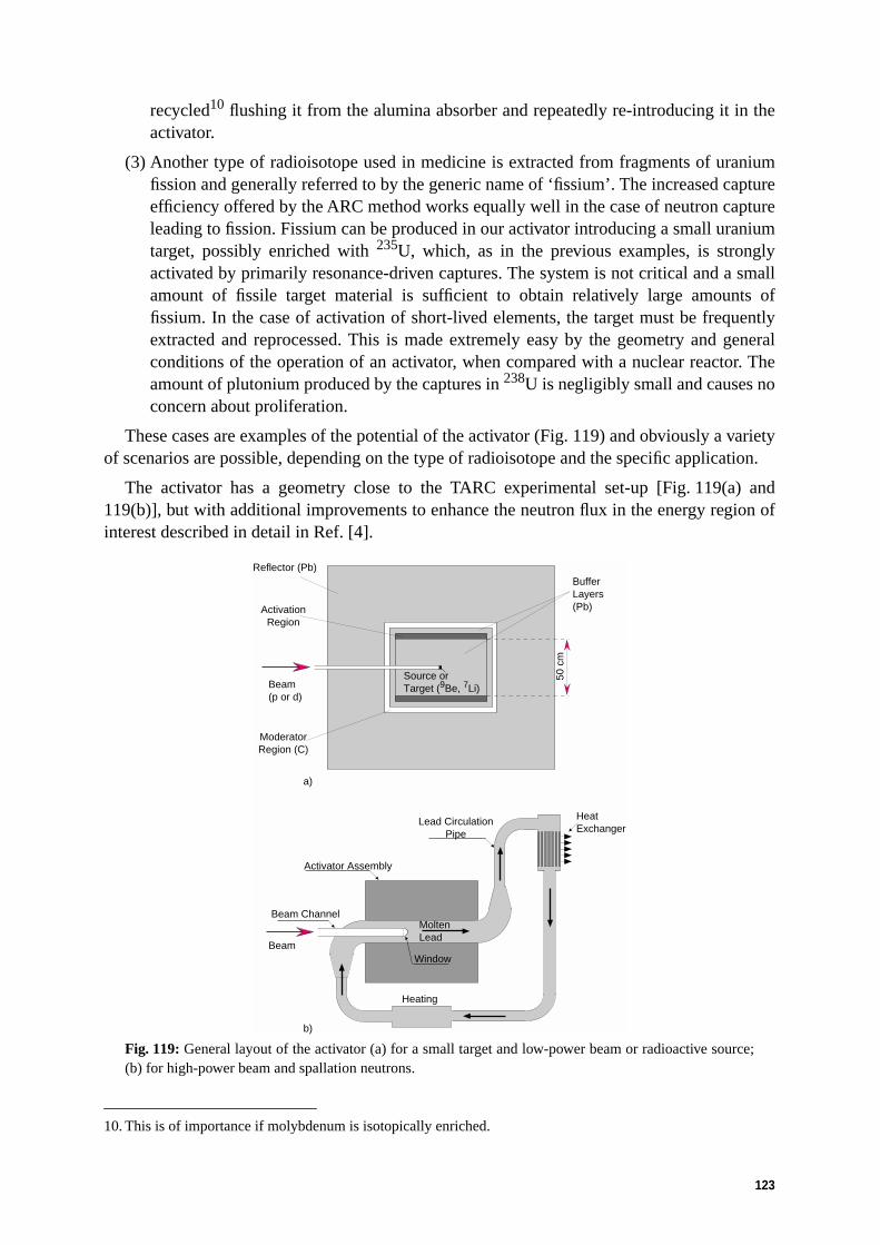
123

recycled10 flushing it from the alumina absorber and repeatedly re-introducing it in theactivator.

(3) Another type of radioisotope used in medicine is extracted from fragments of uraniumfission and generally referred to by the generic name of ‘fissium’. The increased captureefficiency offered by the ARC method works equally well in the case of neutron captureleading to fission. Fissium can be produced in our activator introducing a small uraniumtarget, possibly enriched with 235U, which, as in the previous examples, is stronglyactivated by primarily resonance-driven captures. The system is not critical and a smallamount of fissile target material is sufficient to obtain relatively large amounts offissium. In the case of activation of short-lived elements, the target must be frequentlyextracted and reprocessed. This is made extremely easy by the geometry and generalconditions of the operation of an activator, when compared with a nuclear reactor. Theamount of plutonium produced by the captures in 238U is negligibly small and causes noconcern about proliferation.

These cases are examples of the potential of the activator (Fig. 119) and obviously a varietyof scenarios are possible, depending on the type of radioisotope and the specific application.

The activator has a geometry close to the TARC experimental set-up [Fig. 119(a) and119(b)], but with additional improvements to enhance the neutron flux in the energy region ofinterest described in detail in Ref. [4].

Fig. 119: General layout of the activator (a) for a small target and low-power beam or radioactive source;(b) for high-power beam and spallation neutrons.

10. This is of importance if molybdenum is isotopically enriched.

Beam Channel

Window

MoltenLead

Lead CirculationPipe

Heating

Activator Assembly

HeatExchanger

Beam

Beam(p or d)

Source orTarget (9Be, 7Li)

50 c

m

BufferLayers(Pb)Activation

Region

Reflector (Pb)

ModeratorRegion (C)

a)

b)

124

9.1.3 Characterization of the spallation neutron source

The energy spectrum of the initially produced neutrons is relatively unimportant, since theinelastic processes in the diffuser quickly damp the neutron energy down to about 1 MeV,where the lethargic slow-down of the neutrons is taking over. Therefore, the neutron captureefficiency for activation and, more generally, the geometry of the activator are relativelyindependent of the details of the realization of the source.

In the case of the activation of natural iodine, it is likely that a small sample — of the orderof a fraction of a gram — must be activated for each exposure to a level requiring a cyclotronor similar accelerator with a neutron production rate of a few times 1013 neutrons/second overthe full solid angle. This can be obtained with a proton energy of the order of 10–30 MeV anda current of the order of milliamperes, which is also suited for production of isotopes for PETexaminations. Therefore a combined facility may be envisaged.

In the case of a large industrial production of radionuclides, like for instance 99Mo (99mTc),131I, or of fissium from uranium fissions it may be worth considering similar currents buthigher proton energies, in the region of a few hundred MeV. Activation can then be performedwithin much smaller samples which is a considerable advantage especially in the case ofportable 99Mo (99mTc) dispensers.

At the other end of the scale, the production of small activation with a simple device using aneutron-emitting radioactive source is worth mentioning, since it might be of interest forapplications in which a very weak source (<< mCi) of radioisotopes is needed. This would becheap and simple to operate.

The overall neutron yield from a thick Be target bombarded with a beam of protonsat Ep = 23 MeV is 1.66 × 1014 n/s/mA (E > 0.4 MeV), corresponding to a neutron flux of0.654 × 1012 cm–2 s–1 mA–1 at r = 20 cm from the source, according to the formulaφ(r) ≈ S0/4πDr, which exhibits the lead enhancement factor (D = 1.01 cm). We note also thatthe flux is falling like the inverse of the distance (1/r), more slowly than in empty space wherethe flux is proportional to the solid angle from the source (1/r2). We note that for a current of10 mA, typical for modern cyclotrons, our system leads to the remarkable flux6.5 × 1012 cm–2 s–1, typical of a nuclear reactor. Other target materials can be used, inparticular 7Li, with comparable yields. The neutron yield is a growing function of the protonenergy and for a given beam power is rising proportionally to . Neutrons can beproduced also with other incident particles, in particular deuterons and alphas. For a givenincident energy, the forward neutron yield of deuterons is substantially higher than for protons,but, as relevant in our application, the angle integrated flux is comparable to that of protons[81]. The yield for incident α-particles is substantially lower. In view of the associatedsimplicity and their high neutron yield, proton beams seem to be optimal for the presentapplication.

Neutron yields achievable by proton accelerators and different targets are summarized inFig. 120.

9.1.4 Performance of a typical activator

Transmutation rates (Fig. 121) are largely independent of the chemical binding and isotopiccomposition of the materials inserted in the activator. They are also almost independent of thesource geometry and of the process used for the neutron production, provided their energy isinitially sufficiently high (> 0.4 MeV). More details can be found in Ref. [4].

E00 886.

125

Fig. 120: Neutron yield, S0 per mA of proton current, as a function of the kinetic energy of the protonbeam for both a beryllium target and a heavy spallation target (taken from Ref. [4]).

Fig. 121: Asymptotic activated yield for different elements, as a function of the strength S0 of the neutronsource. Points (1) and (2) correspond to a local production scenario, and points (3) and (4) to a regionalindustrial scale scenario (taken from Ref. [4]).

9.2 Measurement of 99mTc production rate from natural molybdenum

9.2.1 Sample configuration and preparation

The sample used is a standard commercial 99.985% pure sample of molybdenum with veryfew impurities at the 10–3 level which can be ignored. The molybdenum sample was packagedin a small polyethylene bag to facilitate handling during irradiation in TARC. It had the shapeof a thin disk of diameter 12.75 ± 0.05 mm, a thickness of approximately 0.078 ± 0.002 mmfor a total weight of 90.3 ± 0.15 mg. The sample contains 21.79 ± 0.04 mg of 99Mo (Table 26).

1011

1012

1013

1014

1015

1016

1017

0 50 100 150 200 250

Thick Be Target

Spallation Pb (-Bi ) Target

Proton beam energy (MeV)

S0

(neu

tro

ns/

s/m

A)

0.001

0.01

0.1

1.0

10

100

1000

1013 1014 1015 1016 1017

Source neutron yield (n/s)

Beryllium Target Spallation source

127I → 128I

3

4

98Mo → 99Mo

130Te → 131I

1

2

Asy

mp

toti

c ac

tiva

tio

n (

GB

q/g

)

126

Table 26: Properties of the molybdenum sample irradiated in TARC

9.2.2 Molybdenum capture and decay schemes

9.2.2.1 Molybdenum transmutation scheme

Through neutron capture, stable 98Mo is transmuted into 99Mo (Fig. 122), which decayswith a half-life of 65.94 hours into mostly (Br = 87.5%) 99mTc (t1/2 = 6.01 h), but alsosometimes (12.5% of the cases) into 99Tc (t1/2 = 2.111 × 105 yr). 99mTc decays almost always(99.996% of the cases) into the 99Tc ground state through internal transition.

Fig. 122: Neutron capture on 98Mo and subsequent decay scheme.

For 100Mo the scheme is simpler (Fig. 123). 101Mo (t1/2 = 14.61 min) is produced whichdecays 100% of the time into 101Tc (t1/2 = 14.22 min) which itself decays into stable 101Ru.

The 92Mo neutron capture cross-section is relatively small. In our sample of naturalmolybdenum, 92Mo corresponds to only 2.5% of all the captures. For 92Mo, most of thecaptures (> 77%) produce 93Mo (Fig. 124) which has a long half-life and does not contributevery much to the total sample activity. In less than 23% of the cases, 93mMo is formed. As aresult the contribution to the overall sample activity is negligible. It is confirmed by the γspectra where we do not see any significant γ peaks from 93mMo. 93Mo has only X-rays, and93mMo three significant γ’s [69]: 263.1 keV (56.7%); 684.7 keV (99.7%), and 1477.1 keV(99.1%).

ElementFraction

(%)Mass(mg)

Error(mg)

92Mo94Mo95Mo96Mo97Mo98Mo100Mo

14.84

9.25

15.92

16.68

9.55

24.13

9.63

13.40

8.35

14.375

15.08

8.625

21.79

8.696

0.02

0.014

0.02

0.025

0.015

0.036

0.015

Total 100.00 90.3 0.15

99Mo (t1/2 = 65.94 h)

99Tc (t1/2 = 2.111 × 105 yr)

99mTc (t1/2 = 6.01 h)

99Ru (stable)

99.996% IT 0.004% β–

100% β–

β–~ 87.5%

β–~ 12.5%

n + 98Mo (stable) 99Mo (t1/2 = 65.94 h)

127

All the other isomers (94Mo, 95Mo, 96Mo and 97Mo) are irrelevant in this study, since eachof them produces, through neutron capture, another stable element. They do not contribute tothe activation of the sample. We conclude that the total activation of natural molybdenumshould be dominated by the production of 99Mo, with a small contribution from the productionof 101Mo and a negligible contribution from the production of 93mMo and 93Mo. This is indeedconfirmed by our measurements.

Fig. 123: Neutron capture on 100Mo and subsequent decay scheme.

Fig. 124: Neutron capture on 92Mo and subsequent decay scheme.

9.2.2.2 Other neutron reactions

Other possible channels with high-energy neutrons include (n,2n) reactions which canproduce 91Mo (t1/2 = 15.49 min) and 91mMo (t1/2 = 65.0 s) from 92Mo. In the same way 93Moand 93mMo can be produced from 94Mo and finally 99Mo can be produced from 100Mo. Allthese reactions have relatively high neutron energy thresholds (≥ 10 MeV), and represent avery small fraction of the captures, which can be safely neglected. This was checked explicitlywith our simulation.

9.2.2.3 Gamma branching ratios in molybdenum isotopes

Tables 27–28 give the values of the branching ratios, for the various gamma lines used todetect the decays of the isotopes of interest. The branching ratio is defined as the probability ofproducing a given gamma in the decay of the element considered.

101Mo (t1/2 = 14.61 min)β–(100%)

n + 100Mo (t1/2 = 1.2 × 1019 yr) 101Mo (t1/2 = 14.61 min)(n.a. 9.63%)

101Tc (t1/2 = 14.22 min) 101Ru (stable)β–(100%)

93Nb (stable)

99.88% IT 0.12% EC

100 % EC

n + 92Mo (stable)

93Mo (t1/2 = 4.0 × 103 yr)

93mMo (t1/2 = 6.85 h)< 0.006 barn

0.02 barn

93Mo (t1/2 = 4.0 × 103 yr)

93mMo (t1/2 = 6.85 h)

128

Table 27: γ branching ratios in 99Mo decay [69]

(*) Note on the 140.5 keV γ branching ratio: This γ comes mainly from the 99mTc daughterof 99Mo. But 99Mo also produces this line directly. The first number given in Table 27 (90.7%)is taken from Ref. [69] which claims that this is the value at ‘transient’ equilibrium calculatedas:

(60)

where IE is the 140 keV abundance observed in the case of transient equilibrium,

ID ≡

is the 140 keV abundance of the same transition in the decay of the daughter alone. λP and λDare the decay constants of the parent and daughter respectively, and Br is the branching ratiofor the decay from parent to daughter.

The result is clearly different from the 90.7% given in the data tables [69]. We suppose thatone should add the 140.5 keV γ’s not coming from 99mTc according to:

. (61)

From this we obtain = 6.3%. Unfortunately, when we compute that branchingratio directly from the level scheme [63] we get 2.99%. It will be shown later that the 6.3%value gives an activity more consistent with the other lines, therefore, we use that value, but weattribute a large error to it, namely 6.3% ± 3.3%.

Table 28: γ branching ratios in 99mTc decay [69]

9.2.2.4 Correction for extended source geometry and gamma absorption

The activity of the various γ lines of interest was measured, using the same Ge counter asfor the iodine study [68]. The Ge calibration was performed with a naked point-like source,therefore, we need to calculate corrections to take into account that (a) the molybdenum

99Mo lines (keV) Branching ratio (%) Error (%)

140.5181.1366.5739.4777.8

90.7/6.3(*)6.081.1612.144.36

1.8/3.30.120.040.10.11

99mTc lines (keV) Branching ratio (%) Error (%)

140.5142.6

87.70.041

0.140.00025

I IE EquilibriumObserved

DD

D P

99 mBr Br Mo Tc≡ = ×−

× →( )= × ×

× − ×× =

−

− −

λλ λ

99

5

5 60 8773 2037 10

3 2037 10 2 9199 100 875 0 844.

.

. .. .

Brm Tc99( )

Br Br Br Br Mo TcEquilibrium

Observed Mo Tc D

D P

mm

= + ×−

× →( ) ( )99 9999 99λ

λ λ( )

BrMo99( )

129

sample is an extended source of γ’s and (b) that the γ’s produced can be absorbed in themolybdenum sample itself. In this case, we removed the plastic holder to perform the Gecounter measurement (Fig. 125). Absorption in the Ge counter material (aluminium window,etc.) is common to the Ge calibration procedure and to the data taking.

Fig. 125: Details of the set-up used for the measurement of the molybdenum activation, on the TIS Gecounter.

The correction factor, evaluated with the MCNP Monte Carlo code [66], takes into accountalso the correction needed to go from the point-like source used in the efficiency calibration ofthe Ge counter, to the extended sample geometry. In both cases the corrections are expected tobe small, of only a few per cent. We followed the procedure used in the analysis of the 129Iactivation [68], where we defined the Ge effective efficiency to be used in the analysis as:

(62)

where the correction to the measured point-like efficiency can be defined as:

(63)

The results summarized in Table 29 are taken partially from Ref. [82], for all the γ’s ofinterest here. Note that the systematic uncertainty for the low-energy γ’s (below about500 keV) may be larger than the canonical 5% because relatively few points were available inthe calibration.

The error on the efficiency correction (Table 29) is estimated to 50% of the correction butdoes not matter very much because it is small in absolute value compared to the error on themeasured efficiency which suffers from the precision on the activity of the calibration sources(5%) and on the interpolation procedure between measured points (5%).

9.2.2.5 Correction for gamma overlap

It is apparent from the excited level properties of 99Tc, that some of the gamma lines used inthis analysis are correlated with one another, both in time and in space. Therefore, there is acertain probability that two or more gammas are recorded together in the same Ge counter.When this happens, the observed energy is not in the peak corresponding to the gammasconsidered, and the event does not contribute to the peak counting. We estimate, based on acalculation made with MCNP [66], that this effect is smaller than in the case of 129I where itwas at most 6%. In the following analysis we neglect this effect, since it is small compared toseveral sources of systematic errors.

MolybdenumSample

D1

2 m

m

1 m

m

Plexiglass

ε εεεeff measured

point-like simulatedsample

simulatedpoint-like≡ ×

Correction simulatedsample

simulatedpoint-like≡ −1

εε

130

Table 29: Effective γ efficiency of the TIS Ge counter used at position D1 (all Ge counter measurementswere made at position D1). The correction is defined above

9.2.3 General summary of the irradiation data

The activation was performed in TARC in hole 10 at z = +7.5 cm (2172 PS shots,2.156 × 1013 ± 3.6 × 108 (stat.) protons. The number of non-empty shots was 2075 and themeasured mean distance of the beam impact to the beam axis was 2.84 mm

9.2.4 Data analysis

9.2.4.1 Production of 99Mo and of 99mTc

The procedure is totally analogous to the one used for the irradiation of 129I and is describedin detail in the corresponding note [68]. The run history for irradiation number 1 is given inFig. 126.

Fig. 126: History of beam intensity for run 767.

Assuming that at a given position in the lead assembly, Ni atoms of 99Mo are produced per109 incident protons, we can calculate the number of 99Mo and of 99mTc atoms present at theend of irradiation in the following way:

Gamma lines (keV)Measured

efficiency (%)Correction (%)

Effective efficiency (%)

140.5

181.1

191.9

366.5

505.9

590.9

739.4

777.8

1012.5

3.39

2.83

2.70

1.43

1.04

0.908

0.729

0.689

0.530

2.5

2.4

2.3

1.9

1.5

1.2

0.8

0.7

0.37

3.30

2.76

2.64

1.41

1.03

0.897

0.723

0.684

0.530

0.0×100

2.0×109

4.0×109

6.0×109

8.0×109

1.0×1010

1.2×1010

1.4×1010

1.6×1010

1.8×1010

0 500 1000 1500 2000

Run 767

PS shot number

Nu

mb

er o

f p

roto

ns

per

PS

sh

ot

131

(64)

(65)

where Xn is the number of protons (in units of 109 protons) in PS beam shot n, λ1 = 2.91994 ×10–6 s–1 is the decay constant of 99Mo, λ2 = 3.203675 × 10–5 s–1 is the decay constant of99mTc, tend is the time of the last PS shot, tn is the time of shot number n, Br is the probabilitythat 99mTc is formed in the decay of 99Mo, taken to be 87.5%. The quantitiesA ≡ N(99Mo)end/Ni which we call the 99Mo beam integral, and B ≡ N(99mTc)end/Ni which wecall the 99mTc beam integral characterize a given irradiation and are given in Table 30.

Table 30: Beam integrals (A, B) calculated for each of the processes. These beam integrals characterize theproduction and decay of 99Mo, and 99mTc during the irradiation. The errors include the systematic errorscoming from the absolute beam calibration (5%) and the statistical error (but, negligible in all cases).

9.2.4.2 Gamma spectra analysis

The time measured between the last PS shot and the beginning of Ge counting is1867 seconds and the measurement lasted 10 000 seconds.

The number of counts in the γ peaks (Table 31) was determined in three ways: (a) using thestandard algorithm available on the Ge system we used (TIS); (b) using an algorithmdeveloped by our group for the rabbit analysis and based on Ref. [61]; and (c) making a fit withinteractive software (PAW) [83], in cases of ambiguity of results from (a) and (b). This allowedus to compare the algorithms, and gave us a way to correct technical problems and estimate thesystematic errors. Figure 127 shows the Ge gamma spectrum obtained.

Table 31: Peak-finding results for 99Mo data (the errors are statistical only)

A good technical overall test of (a) the peak-fitting performance; (b) the estimation of theGe counter acceptance; (c) the effect of γ overlap; (d) the determination of the γ-line branchingratio is obtained by making sure that all the γ-lines of one element give the same activity. Thisis indeed the case for 99Mo (Fig. 128). Since, in the case of 99Mo, there are five different γ lineswhich we can use, the spread between the activities obtained from these lines, is a goodmeasure of the systematic error. We find a standard deviation of 6% (Table 31), which is thevalue we are using in our general error analysis.

Activation Run A ∆A B ∆B

1 767 20464.8 1000 621.46 31

E (keV) Counts Error

140.51181.09366.42739.5777.91

161541804158888313

13152213218

N N X e t t

n

n N

( Mo)end i nend n99

1

1= × − −( )=

=∑ λ

N N X e et t t t

n

n N

( )99 1

2 1 1

1 2mend i nTc

Br[ ]end n end n= ×

−× −− −( ) − −( )

=

=∑λ

λ λλ λ

132

Fig. 127: Ge gamma spectrum taken shortly after the end of irradiation, showing the 99Mo, 99mTc, 101Mo,and 101Tc peaks of interest.

Fig. 128: Measurement of capture rates on 98Mo from the activity of each 99Mo gamma line (statisticalerrors only).

9.2.4.3 Calculation of the 98Mo capture rates

We call n1(t) and n2(t) the number of 99Mo and 99mTc atoms at time t, and n1(0) and n2(0)the numbers of atoms of these two elements at time t = 0, defined as the time of the last PS shotin the irradiation run. We have:

(66)

10

100

1000

10000

100 200 300 400 500 600 700 800 900 1000 1100

99mTc99Mo

99Mo

99Mo

99Mo

101Tc

101Mo101Mo 99Mo

101Mo

101Mo

Photon energy (KeV)

Co

un

ts

0

200

400

600

800

1000

1200

1400

1600

1800

2000

0 100 200 300 400 500 600 700 800

First activation: 98-Mo captures

Gamma energy (keV)

Cap

ture

s p

er 1

09 p

roto

ns

n N A N

n N B N

199

299

0

0

( ) = ( ) ≡ ×

( ) = ( ) ≡ ×

Mo

Tc

end i

m

end i

133

where A and B are the beam integrals given in Table 30. The expressions for n1(t) and n2(t) aregiven by:

(67)

where Br is the fraction of 99Mo decays into 99mTc. With these expressions we can calculatethe number of decays for each element in a time window [Age, Age + Tc], where Age is the timeat which the Ge counting starts, and Tc is the counting time:

(68)

from which we can obtain the number of 98Mo captures per 109 protons, from the number ofGe counts in a given γ peak in the 99Mo decays [Ncounts(γ)] (except for the 140.5 keV linewhich has to have special treatment):

(69)

The 140.5 keV γ line gets contributions from both 99Mo and 99mTc, and therefore thenumber of captures per 109 protons calculated with this line is a bit more involved:

(70)

The number of captures obtained from each line is given in Table 32. The average capturerate is found to be 1785 ± 46 (stat.) (Table 32). Taking into account, in addition, the systematicerrors of 10.7% (Table 34) we get Ni = 1785 ± 191 (tot.), to be compared to the Monte Carloprediction of 2016 ± 126 where the error is statistical only.

Several technical checks of the evaluation of the number of captures are described inRef. [8].

Table 32: Measured rates of captures on 98Mo from each gamma line

Gamma energy (keV) Ni (capt/109 protons) Statistical error

140.51181.09366.42739.5777.91

Weighted average

1841.91833.61651.31727.51793.91785

139532246310346

n t n e

n tn

e e n e

t

t t t

1 1

21 1

2 12

0

00

1

1 2 2

( ) = ( )

( ) = ( )−

−[ ] + ( )

−

− − −

λ

λ λ λλλ λ

Br

N n e e

Nn

e e nn

e e

Age T

Age T Age T

1 1

22 1

2 12

1 1

2 1

0 1

01 0

01

1 1

1 1 2 2

decay

decay

c

c cBr Br

= ( ) −[ ]= ( )

−−[ ] + ( ) − ( )

−

−[ ]

− −

− − − −

λ λ

λ λ λ λλλ λ

λλ λ

NN e

A e

Age

Ticounts

Br c= ( )

−[ ]−γ

ε

λ

γ γλ

1

11

NN

A e eB

Ae e

mTAge T T Age T

icounts

MoBrBr Br Br

Brc

cm

c c

= ( )

+−

−[ ] + −−

−[ ]

− − − −

140 5

1 199

99

1 199

2 22

2 1

1

2 1

.

ελ

λ λλ

λ λγ γγ λ λ

γλ λ

134

9.2.5 Monte Carlo simulation

9.2.5.1 Simulation of capture rates

The simulation (Table 33) [82] was obtained with the same general procedure used in othersimilar analyses in the TARC experiment and is based on the JENDL database formolybdenum neutron cross-sections (Fig. 129).

Fig. 129: Neutron capture cross-sections of stable molybdenum isotopes (from JENDL-3.2).

92Mo

64.9

1b 3

47eV

94Mo

7.73

b 10

8.8e

V

95Mo

5889

b 44

.9eV

96Mo

1879

.3b

131.

4eV

97Mo

642b

70.

9eV 98Mo

60.1

b 12

.1eV

100Mo

24b,

97.2

eV

σ(b

)

10–4

10–3

10–2

10–1

1

10

102

103

E(eV)10–5 10–3 10–1 10 103 105 107

σ(b

)

10–4

10–3

10–2

10–1

1

10

102

103

E(eV)10–5 10–3 10–1 10 103 105 107

σ(b

)

10–4

10–2

1

102

104

E(eV)10–5 10–3 10–1 10 103 105 107

σ(b

)

10–4

10–3

10–2

10–1

1

10

102

103

E(eV)10–5 10–3 10–1 10 103 105 107

σ(b

)

10–4

10–3

10–2

10–1

1

10

102

103

E(eV)10–5 10–3 10–1 10 103 105 107

σ(b

)

10–4

10–3

10–2

10–1

1

10

102

103

E(eV)10–5 10–3 10–1 10 103 105 107

σ(b

)

10–4

10–2

1

102

104

E(eV)10–5 10–3 10–1 10 103 105 107

135

Table 33: Captures per 109 protons, on the various stable isotopes of natural molybdenum contained in theactivated sample, as obtained from the TARC simulation

9.2.5.2 Systematic errors

Table 34 summarizes all the systematic error contributions to the measurement of the 98Mocapture rate and to the Monte Carlo calculation.

Table 34: Sources of systematic errors in the measurement of the number of captures on 98Mo and in theirsimulation

Isotope Captures per 109 p Error (stat.) Fraction (%)

92Mo94Mo95Mo96Mo97Mo98Mo100Mo

373.0325.4

13357.13246.02341.32015.9777.8

545132616113612679

1.661.4559.5314.4710.448.983.47

Error sourceError on error

sourceResulting error on

98Mo captures

Beam intensityGe acceptance (source and systematics of calibration)Molybdenum amount

5 %6.4%0.2%

5%6.4%0.2%

Total common experimental 8.1%

Peak finding and statisticsSample position in Ge systemBr. ratio, Ge acceptance, absorptionT0 measurement

2.6%1.1 mmsee text

15 s

2.6%2.6% (D1)

6%(*)neglig.

Total individual experimental 7%

Total experimental 10.7%

Monte Carlo 98Mo capture cross-section(**) – 7%

Monte Carlo statistics & others (***) 7% 7%

Total Monte Carlo 9.9%

(*) Error estimated from spread of activity measurements for various γ lines in 99Mo decays, which

includes part of the first two sources of errors, hence the estimated total of 6%.

(**) As our estimate of the error due to the uncertainty on the neutron capture cross-section on 98Mo we

take into account the spread of capture rates obtained with the various databases (Fig. 130).

(***) The Monte Carlo error quoted here includes statistical errors and estimates on the error on

geometry, impurity contents, method, etc. We do not include the error which comes from the simulation

of the neutron flux, but only errors belonging to the simulation of molybdenum properties. From TARC

flux measurements we know that the agreement between simulated flux and data is better than 10%

(Fig. 37) on average in the energy range of interest.

136

Fig. 130: Ratio of numbers of 98Mo captures obtained from various data libraries (ENDF/B-VI & JEF-2.2)to the JENDL number, as a function of distance to the centre of the lead volume.

9.2.5.3 Comparison with the data

The 98Mo measured capture rate (1785 ± 191 per 109 protons) is well consistent with theprediction (2016 ± 199 per 109 protons) from the TARC simulation (Fig. 131). The averageratio data/Monte Carlo is 0.89 ± 0.13.

As for all TARC neutron capture measurements, in the Monte Carlo uncertainty, there is inaddition an overall contribution coming from how well the neutron flux is simulated (mainlydue to the uncertainty on the spallation process and on the lead cross-sections, see Section 5).This additional uncertainty is about 15%. This makes our measurement clearly more precisethan the prediction.

Fig. 131: Comparison between the observed capture rate on 98Mo and the simulation (hole 10,z = +7.5 cm). The values are compared for each of the 99Mo gamma lines used in the analysis. The errorbars shown represent the statistical errors of both data and Monte Carlo simulation. The thick horizontalline is the average ratio. The band shows the total common error (0.11) centred on 1.

0.8

0.85

0.9

0.95

1

1.05

1.1

0 20 40 60 80 100 120 140

ENDF/B-VI/JENDL

JEF-2.2/JENDL

98Mo

Rat

io t

o J

EN

DL

Distance to centre (cm)

0

0.1

0.2

0.3

0.4

0.5

0.6

0.7

0.8

0.9

1

0 100 200 300 400 500 600 700 800

First Activation: 98Mo captures

Gamma energy (keV)

Rat

io d

ata

/ Mo

nte

Car

lo

137

9.2.6 Various checks on the data

We have used the various Ge counting measurements, made after a high-intensityirradiation, to verify the quality of some of the basic data used in this analysis. The Gecounting data can be used to study the production of 99mTc and obtain information on thehalf-life of the various elements involved.

Using for instance the 181 keV line of 99Mo, we can fit the average observed counting timeas a function of the age of the sample. We get t1/2 = 65.7 h (Fig. 132), in excellent agreementwith the 65.94 h given in the NNDC/BNL library.

Fig. 132: Determination of the 99Mo half-life, using the 181 keV line. The average counting time is plottedversus the sample age at beginning of counting.

It is clear that the 140.5 keV line is mainly produced by 99mTc. We can estimate the numberof 99mTc atoms present in the sample as a function of time (Fig. 133). The maximum numberof 99mTc atoms occurs at time tmax ~ 5 hours, given by:

(71)

and is nicely consistent with what we observe (Fig. 133). The 191 keV line of 101Mo was usedto obtain a check of the 101Mo half-life (Fig. 134). We find t1/2 = 14 min 45 s ± 20 s to becompared to 14 min 37 s given in the NNDC/BNL database.

9.2.7 Conclusion

We have verified that 99mTc could be produced simply by activation of natural molybdenumproducing 99Mo from 98Mo.

The overall activity of natural molybdenum after activation is dominated by the productionof 99Mo; the isomers other than 98Mo induce only a small contribution to the overall activity(mainly from 101Mo).

The rate of neutron capture on 98Mo, hence of production of 99mTc, is found to beconsistent with the TARC simulation prediction and therefore validates this simulation for thisparticular process.

0×100 2×105 4×105 6×105 8×105 1×106 1.2×106

Sample age (s)

106

105

104

Ave

rag

e ra

te o

f 18

1 ke

V li

ne

t

n

nmax

ln

=−

−( ) ( )( )

−

λλ

λ λ λλ

λ λ

2

1

2 2 1 2

12

1

2 1

0

0 Br

138

Fig. 133: Number of 99mTc atoms present in the sample, as a function of time, following the thirdactivation.

Fig. 134: Determination of 101Mo half-life, using the 191 keV line and data from activation number 3.

10 Energy Deposition in Lead by Neutrons

10.1 Introduction

When a proton beam hits the TARC lead volume, a large number of particles, mainlyneutrons, but also photons and charged particles are produced. These particles move around inthe lead inducing different scattering processes, some of them producing energy that heats upthe lead. The amount of heat generation by neutrons is normally much smaller than the heatdeposited by the protons through cascade and ionization, but it is nevertheless very interestingboth from the characterization of the spallation and diffusing cascades and from the practicalpoint of view as a direct measurement of total energy deposited at different positions close tothe spallation target. Calorimetric measurements of such energy deposition in a lead sampleplaced inside the TARC assembly were performed in August–September 1996. The energy, E,

0.0×100

2.0×1015

4.0×1015

6.0×1015

8.0×1015

1.0×1016

1.2×1016

1.4×1016

0×100 1×105 2×105 3×105 4×105 5×105 6×105 7×105 8×105 9×105 1×106

Sample age (s)

Nu

mb

er o

f 99

mT

c at

om

s

100

1000

0 500 1000 1500 2000 2500 3000 3500

101Mo Half -Life

Sample age (s)

Ave

rag

e co

un

tin

g r

ate

139

was obtained by a calorimetric method in adiabatic conditions: by measuring the temperatureincrease, ∆T, exhibited by a sample with known heat capacity, C(T), then:

E = C(T) ∆T ; assuming ∆T<<T . (72)

At room temperature, ∆T values are expected to be only some tens of microkelvin for a totalheating time of one hour [84]. Therefore, the measurements had to be performed atliquid-helium temperature (about 4 K) since the specific heat of lead decreases rapidly as thetemperature is lowered. At 4 K the specific heat of lead is 180 times smaller than the value atroom temperature, so the ∆T values should typically be a few millikelvin. Our experimentalset-up (Fig. 135) achieved a temperature resolution of 0.2 mK which allowed reliablemeasurements of the energy deposition.

Fig. 135: Schematic description of the different parts and materials of the cryostat.

10.2 Experimental set-up

A home-made cryostat (Fig. 135) designed and built in the Laboratorio de BajasTemperaturas of the Universidad Autónoma de Madrid was used in the measurements. Thecryostat is part of a continuous flow system of liquid 4He. Liquid helium is transferred from thehelium dewar into the cryostat through a double jacket siphon. The helium gas produced byevaporation in the cryostat returns through the external jacket of the siphon, thus refrigeratingit. The flux and base temperature are controlled with the aid of a pump and a needle valve.Typical working flows are of 1.25 �/h. It takes several hours for the sample to reach lowenough temperatures. The base temperature in the experiment was about 4.15 K. Temperaturefluctuations of some tenths of kelvin with a period of some tens of seconds can appear in thebath, although normally, the stability is better than 2 mK.

As the measurements are performed under adiabatic conditions, it is necessary to gethigh-quality vacuum; using a turbomolecular pump the level reached was typically 10–8 bar.Two radiation shields made of copper prevent thermal radiation exchange with thesurroundings, the inner one is in good thermal contact with the bath at 4 K.

External can (stainless steel)L = 22.5 cm. fl 5.0 cmThickness 0.2 mm

External radiation shield (copper)L = 20 cm. fl 4.0 cmThickness 0.3 mm

Inner radiation shield (copper)L = 10 cm. fl 2.8 cmThickness 0.3 mm

Brass barL = 9.5 cm. fl 0.6 cm

Nylon threadsL = 2.0 cm. fl 0.015 cm

Ge thermometer(GR200)

Manganin wiresfl 0.005 cm.Total Length = 30.7 cm

Samples: a) Pb #1 L = 2.5 cm. fl 1.4 cm. M = 42.167 g b) Pb #2 L = 1.5 cm. fl 1.4 cm. M = 24.440 g c) Cu L = 2.5 cm. fl 1.4 cm. M = 32.078 g

Cooper blockL = 0.5 cm. fl = 2.6 cm.

Heat exchanger(copper with

circulating He)

Carbon glassthermometer

Liquid He inlet

He outlet(liquid+vapour)

140

The sample hangs from an eccentric brass bar by two nylon threads to keep it underadiabatic conditions; the cooling power of these threads is less than 20 nW/K. The inner shieldis also used to cool the sample down to the copper shield temperature (~ 4.2 K): by rotating thewhole cryostat, the sample can be put in thermal contact with it. The thermometer is placedinside a hole made in the sample, and clamped by a screw. Its manganin leads are clamped tothe thermal bath container at different places. They are finally fixed to the sample with varnishto avoid erroneous measurements of temperature. The cooling power of the leads is less than20 nW/K. The thermometer Joule heating power is less than 10 nW. Two differentthermometers were used: a doped germanium chip and a carbon glass resistance. Both aremounted strain-free in a gold plated copper can, with internal atmosphere of 4He and sealed byan epoxy heat sink.

In these quasi-adiabatic conditions, the leak time of the energy between the bath at 4.5 K tothe sample is more than 20 hours. For this reason, the fast temperature fluctuations thateventually appear in the bath are not seen by the sample. So, even when the bath temperature isnot very stable, good calorimetric results can be obtained. The resolution in the temperature ofthe sample is about 0.2 mK. As the specific heat of lead at 4 K is 7 × 10–4 J/K/g, this allowsone to measure energy productions of the order of 200 nJ/g.

The specific heat of the sample was measured between 4 K and 8 K. The estimated error inthe region of interest, i.e. below 6 K, is 3%. During the calibration procedure the conditionsinside the TARC assembly were simulated: the sample was heated by Joule dissipation pulsesin an electrical resistance, which was in good thermal contact with the sample. The amount ofenergy of these pulses was fixed at similar values to those expected from prior Monte Carlosimulation results.

10.3 Analysis of the data

The measurements were mostly performed under adiabatic conditions, although anon-adiabatic experiment was also done. The results in these different conditions areconsistent. In what follows, we will distinguish between quasi-adiabatic and non-adiabaticmeasurements.

10.3.1 Analysis of the data in quasi-adiabatic conditions

In the adiabatic experiments we measure the temperature of the sample when protons areinjected into the lead assembly, and also both before and after the proton injection period. InFig. 136, curve 1 shows the evolution of the temperature of the sample versus time in thesethree regimes. The two small kinks at about 0.57 hours and 1.34 hours, correspondingrespectively to the start and end of the beam activation, show that the beam is indeed heatingthe sample. Nevertheless, even when there is no beam, the temperature changes smoothly. Atypical rate in our case was +0.05 K per hour.

This indicates the presence of an extra source of heat whose power is about 400 nW. Thisvalue is bigger than the heating power due to neutrons and other particle interactions in most ofthe measurements. In the calibration procedure it was realized that the heating rate wasproportional to the intensity of mechanical vibrations. These vibrations cannot be reduced tozero, because some of them come from the flux of helium inside the cryostat. The temperatureincrease of the sample at time t is then:

∆T = T(t) – T(0) = ∆Tp(t) + ∆Tv(t) . (73)

141

Fig. 136: Analysis of data for an adiabatic measurement: (1) Typical time evolution of the temperature ofthe sample; (2) Heating rate versus temperature. The dashed line is a second-order polynomial fit of thederivative using the data when the beam is off; (3) Increase in temperature due to the energy released whenthe proton beam is turned on, after subtraction of the general temperature drift.

∆Tp(t) corresponds to the proton pulses, ∆Tv(t) is due to mechanical vibrations. The netextra heating power seen in the experiment depends on various parameters: the difference intemperature between the bath and the sample, the position of the sample, the mechanicalvibrations, the vacuum, and so on.

All these parameters change in every measurement. To obtain ∆Tp it is necessary todetermine and subtract ∆Tv. We have used the following expression for the time evolution ofthe temperature of the sample:

. (74)

T s

amp

le (

K)

t (h)

firstpulse

lastpulse

RUN 885

Hole 1; Z = 67.5 cmD(cm) = 124.8 cm∆T = 3.2 mK

( 1 )

( 2 )

( 3 )

0.040

0.050

0.060

dT

/ d

t (K

/h)

T sample ( K )

Experimental dT/dt

Second order fit of dT/dt

t (h)

∆Tp

= [

T(t

)-T

(0)-

∫ d

T(t

’)/d

t’ .

dt’

] (

K)

0.000

0.001

0.002

0.003

0.004

0.0 0.2 0.4 0.6 0.8 1.0 1.2 1.4 1.6 1.8 2.0

4.30 4.32 4.34 4.36 4.38 4.40

4.30

4.32

4.34

4.36

4.38

4.40

0.0 0.5 1.0 1.5 2.0

T t TT

tt

t( ) ( )= +

′′∫0

0

dd

d

142

When the beam is off, at any time, and ∆Tv(t) is simply:

(75)

where dTOFF/dt means the heating rate when there is no beam. Then, using relation (2) theincrease of temperature due to the beam is:

. (76)

In principle the derivative dTOFF/dt is smooth and continuous with T. When the beam is offdTOFF/dt can be obtained numerically.

Then, for new situations when the beam is off, it can easily be determined by fitting; on theother hand, for situations with the beam on, the value can be obtained by interpolation. Thisprocedure, i.e. the fit of the heating rate dTOFF/dt when the beam is off versus T, is shown inFig. 136, curve 2. Since T depends on time, dTOFF/dt = dTOFF(T(t))/dt also depends on time, andthe integral in Eq. (75) has to be done numerically.

If we plot the result of this correction against time, we obtain directly the temperatureincrease of the sample due to the proton source, see Fig. 136, curve 3. In this figure, thegoodness of the fit is explicit: before and after the proton pulse interval

is zero as expected.

Knowing the specific heat of the sample and the number of protons supplied, we cancalculate the energy deposited per gram and per proton using Eq. (72).

10.3.2 Analysis of the data in non-adiabatic conditions

It is possible to measure the energy even with the sample in thermal contact with the bath. Ifthe beam is on, the sample temperature rises up to a value determined not only by the energylosses in the sample, but also by the thermal exchange between sample and bath. This dependson the contact area and mass of the sample as main parameters.

Eventually, the sample reaches equilibrium and its temperature is stable. When the protonsource stops, the temperature decreases and, following this decay, we can extract the powersupplied to the sample. If the cooling power of the contact is linear with the difference oftemperatures between bath and sample, ∆T(t) should be exponential in time. This is a goodapproximation because the temperature difference is less than 0.1%:

∆T(t) = ∆T0 exp(–t/τ) in which τ = C ∆T0/P , (77)

where C is the heat capacity of the sample and P the heating power of the proton source. Thevalue C is known and P can be obtained by fitting of the experimental data. Since P and thenumber of protons per second are known, the energy deposited per gram and per proton can bederived.

10.4 Experimental results

In all the measurements the protons had a kinetic energy of 2.75 GeV and the beam wasprovided in the fast extraction mode. The beam intensity was measured by two beamtransformers with an absolute precision of 5%, as already explained in previous sections.

d

dpT t

t

( )( )= 0

∆T t

T

tt

t

v( ) =′

′∫d

ddOFF

0

∆T t T t TT

tt

t

pd

ddOFF( ) ( ) ( )= − −

′′∫0

0

d

dp∆T t

t

( )( )

143

10.4.1 Adiabatic measurements

Measurements were performed in four different holes, at several z positions (Table 35).Three different samples and two different thermometers were used. This was done to test theexistence of heating sources different from the protons, and to check possible systematiceffects.

Table 35: Experimental results

Adia- batic data

sample

Thermom. /screw

Run Holez

(cm)D

(cm)

T average

(K)

Cp ×104 (J/g/K)

∆T (mK)

No. of protons(1012)

E×108 (J/g) for 1010 p ∆E = 6%

Big Pb Ge/Brass 763764765

1033

20.020.020.0

49.225.025.0

4.4924.4424.531

9.779.3810.12

5.533.036.5

0.8310.6350.743

6.4848.849.7

Big Pb Ge/Al 878866867868869870871872874875877

881882883884885

886887888890

33333333333 66661

10101010

113.067.552.545.037.530.022.515.07.50.0–6.3

67.522.57.5–5.767.5

37.522.57.5–7.2

114.069.154.647.440.433.527.021.216.815.016.3

90.364.160.560.3124.8

58.650.345.645.6

4.3724.4234.3174.4424.4184.3374.4604.4834.4454.4394.479

4.3094.4354.3524.3364.349

4.3254.4944.3544.322

8.859.238.469.389.198.599.539.719.419.369.68

8.959.338.708.598.66

8.519.808.728.49

4.420.531.526.047.466.277.186.097.8128.9115.5

5.07.18.29.23.2

9.16.89.311.3

1.6281.8141.5791.1571.5811.5941.6491.5011.4291.5861.440

1.6111.4781.5081.6222.060

1.4961.0941.2001.382

2.3910.416.921.127.635.744.655.664.476.077.6

2.794.484.734.871.35

5.186.096.766.94

Big Pb C/Al 943944

33

67.5113

69.1114.0

4.3664.404

8.809.09

6.63.2

0.5791.231

10.052.36

Small Pb

Ge/Al 954 10 37.5 58.6 4.303 8.36 15.5 2.385 5.44

Cu Ge/Cu 892917

1010

67.537.5

81.158.6

4.8195.062

1.371.53

8.62.3

0.1530.035

7.710.2

Non Adia-batic data

sample

Thermom. /screw

Run Holez

(cm)D

(cm)

T average

(K)

Cp ×104 (J/g/K)

∆T (mK)

No. of protons(1012)

E×108 (J/g) for 1010 p ∆E = 6%

Big Pb Ge/Brass 760 10 20.0 49.2 4.129 3.10 1.15 7.99 6.33

144

The first lead sample, of 42.167 g, was measured with both thermometers. No discrepancyis seen although germanium and carbon have very different heat cross-sections. The extraheating supplied by the germanium or carbon in the thermometers is negligible. There is nodifference between this sample and the second (small) lead sample of 24.440 g. Heatingsupplied by the varnish, contact grease, manganin leads, copper can or nylon threads by heatconduction can be neglected, because all these elements were the same in both samples.

There is an exponential dependence of the deposited energy with radial distance (Fig. 137).This dependence is suddenly lost for hole 3 near z = 0. Nevertheless, if we add 4 cm to theassumed z values, and plot the energy versus , the exponentialdependence is recovered for the whole data set (Fig. 137). The decay distances obtained fromthe exponential fits are: 59 cm, 53 cm and 30 cm for holes 6, 10 and 3, respectively. Hole 3, theclosest to the beam, shows a behaviour significantly different from that of the other holes,indicating extra contributions for the energy release in this region of the lead volume (probablythe spallation cascade). A spherical symmetry is inferred from the data obtained far away fromthe beam axis as the measurements in holes 6 and 10 follow a similar radial dependence. Atlarge distances, all curves seem to converge. This is consistent with the fact that far away fromthe centre of the lead volume, the quasi-spherical behaviour has to be recovered for alldirections.

Fig. 137: Experimental data obtained at several holes and z positions. The released energy is plotted versusradial distance to the centre after adding 4 cm to the assumed z coordinates. Different symbols correspondto different experimental configurations.

Lead becomes superconducting below 7.19 K. This fact is reflected in the specific heat,which is lower than the linear extrapolation of normal lead properties down to 4 K. We do notthink that superconductivity had other major influences in the results. Any possibleperturbation is relaxed in a few milliseconds, because the temperature increases are small andthe pulses are very short. Temperature measurement times are in the range of seconds, so wealways measure the temperature when the sample is in equilibrium.

Copper has a much larger heat cross-section. Copper is present in the germaniumthermometer, in the screw used to clamp the thermometer, and in the manganin wires: about150 mg in all. It could then have a significant contribution to the observed energy released in

′ = + + +D x y z2 2 24( )cm

1

10

100

0 20 40 60 80 100 120 140

Modified distance to centre (cm)

En

erg

y re

leas

ed f

or

1010

pro

ton

s o

f 2.

75 G

eV (

J/g

)

Pb in Hole 3 (Ge therm & Al screw)Pb in Hole 3 (Ge term & brass screw)Pb in Hole 3 (C therm & Al screw)Pb in Hole 10 (Ge therm & brass screw)Pb in Hole 10 (Ge therm & Al screw)Small Pb in Hole 10 (Ge therm & Al screw)Pb in Hole 6 (Ge therm & Al screw)

Hole 3

Hole 6

Hole 1

Hole 10

Pb in Hole 1 (Ge therm & Al screw)

145

the sample. Two measurements were performed in hole 10 with a copper sample (Fig. 137).The specific energy dissipation measured in copper is twice that measured in lead. But, as themass of copper is 200 times smaller than the lead mass, its effect can be neglected.

To ensure an optimal thermal contact between the sample and the thermometer, thethermometer lead is pressed with a screw. Unfortunately, lead is too soft to be used for thispurpose. We have used screws of aluminium and brass (70Cu, 30Zn ) of 70 mg. There is noappreciable difference in the measurements done with both materials. As the predicted heatingfor aluminium is much smaller than that of copper, we conclude that the screw has no relevantinfluence on the measurements. In the case of the copper sample, a copper screw was used. Insummary, it is found that the influence of probes in the measured energy can be neglected.

The precision in the determination of positions is about ± 0.3 cm. The accuracy in themeasurement of the increase of temperature is 0.2 mK. The specific heat data have estimatederrors of around 3%. The uncertainty on the beam intensity is 5%. It follows that the precisionin the determination of the specific energy in the adiabatic measurements is typically 6%.Nevertheless, when the increase in temperature is only of a few millikelvin, the error rises to10%.

10.4.2 Contact or non-adiabatic measurements

The analysis of the non-adiabatic measurement is illustrated in Fig. 138. The evolution ofthe bath temperature [Fig. 138(a)] shows that the stability of temperature is within about 2 mK.In these continuous flux systems there are also fast fluctuations of a few tenths of millikelvin.The evolution of the sample temperature [Fig. 138(b)] shows clearly the turning off and on ofthe beam as sudden heating or cooling. Four of these jumps can be seen.

The difference of 2 mK between sample and bath is due to usual calibration errors inabsolute temperature. However, the sensitivity in the measurement of relative temperaturechanges is better than 0.2 mK.

We have subtracted the thermal drift in the bath from the sample temperature in order toobtain the heating due only to the beam [Fig. 138(c)]. As the thermal contact is far from perfect(in this case the relaxation time of the sample heat is about 3 minutes), the thermal noise in thebath is damped in the sample. Anyway, if we compare the sample and bath temperatures, wesee that the temperature in the sample follows the overall evolution of the bath temperature.

From the exponential fit, the relaxation time is τ = 167.2 s. Using Eq. (77), the thermalconductivity is then K = Cp M τ–1 = 1.86 × 10–4 W/K. The heating power is P = K∆T0 = 2.13× 10–7 W. Finally, the energy deposited per gram and per 1010 protons is E = P M–1 Nps

–1 =6.33 10–8 J/g/1010 p. Where Nps is the number of protons per second, in units of 1010 p/s. Thismeasurement was done in hole 10 at z = 20 cm. After comparing with the data obtained inquasi-adiabatic conditions in the same position (E = 6.48 × 10–8 J/g/1010 p), we conclude thatthe agreement between the two methods is quite reasonable.

There are some disadvantages in the non-adiabatic measurements. First, as the heatingobserved is always smaller than in the adiabatic case, measurement precision is worse. Onlyfor positions close to the centre of the lead assembly can the temperature increase be resolvedwith sufficient accuracy. Secondly, as the sample is in mechanical contact with the bath,instabilities can be generated in the sample temperature by both temperature fluctuations andexternal vibrations.

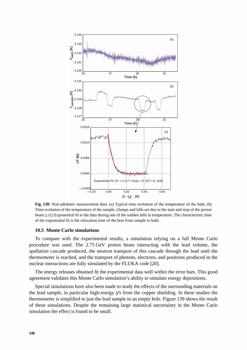
146

Fig. 138: Non-adiabatic measurement data: (a) Typical time evolution of the temperature of the bath; (b)Time evolution of the temperature of the sample. (Jumps and falls are due to the start and stop of the protonbeam.); (c) Exponential fit to the data during one of the sudden falls in temperature. The characteristic timeof the exponential fit is the relaxation time of the heat from sample to bath.

10.5 Monte Carlo simulations

To compare with the experimental results, a simulation relying on a full Monte Carloprocedure was used. The 2.75 GeV proton beam interacting with the lead volume, thespallation cascade produced, the neutron transport of this cascade through the lead until thethermometer is reached, and the transport of photons, electrons, and positrons produced in thenuclear interactions are fully simulated by the FLUKA code [20].

The energy releases obtained fit the experimental data well within the error bars. This goodagreement validates this Monte Carlo simulation’s ability to simulate energy depositions.

Special simulations have also been made to study the effects of the surrounding materials onthe lead sample, in particular high-energy γ’s from the copper shielding. In these studies thethermometer is simplified to just the lead sample in an empty hole. Figure 139 shows the resultof these simulations. Despite the remaining large statistical uncertainty in the Monte Carlosimulation the effect is found to be small.

4.130

4.131

4.132

4.133

4.134

Tb

ath (

K)

(a)

4.127

4.128

4.129

4.130

4.131

Tsa

mp

le (

K)

Time (h)

(b)

—0.0005

0.0000

0.0005

0.0010

0.0015

—0.20 0.00 0.20 0.40 0.60

[t - t0] (h)

∆T (

K)

Exponential Fit: ∆T = 1.217 × Exp(—21.527 × t) (mK)

(c)

25 27 29 31

25 27 29 31Time (h)

147

Fig. 139: Comparison of the FLUKA Monte Carlo results with the experimental data for hole 3. Both thefull geometry and the Pb only simulations are shown.

10.6 Conclusion

We have found that the designed thermometer is a highly precise instrument for themeasurement of small amounts of deposited energies: its resolution is better than 200 nJ. Weexploited the fact that specific heats decrease with decreasing temperature. Going down toliquid-helium temperature, we were able to measure temperature changes that are equivalent toonly a few microkelvin at room temperature.

The energy deposited in a small lead sample placed in different holes at several z positionshas been measured. The measurements were performed in quasi-adiabatic and non-adiabaticconditions, the results from both methods are found to be in good agreement. The influence ofthe probes (thermometers, screws or leads) is found to be negligible as a result ofmeasurements taken with different experimental configurations. The results obtained are ingood agreement with the FLUKA Monte Carlo simulation.

Hole 3, the one closest to the beam, shows a behaviour different from that of the other holes,indicating extra contributions to the energy release in this region of the lead volume (probablythe spallation cascade). A spherical symmetry for long distances seems a good approximationto our data. After shifting by 4 cm the value of the z parameter, the dependence of energydeposition with radial distance becomes exponential for each hole.

The agreement between experimental data and Monte Carlo results validates the physicalparameters used in the simulation. This same validation applies when the program is used tostudy the energy released in lead by the neutron cascade in the Energy Amplifier.

10—8

10—7

10—6

0 20 40 60 80 100 120

Z coordinate + 4 cm (cm)

Sp

ecif

ic e

ner

gy

rele

ase

per

pro

ton

(J/

g)

per

1010

pro

ton

s

TARC Data (Hole 3)

Full Monte Carlo simulation

MC Pb sample only (simplified)

148

11 Practical scheme for an Incineration Device Based on ARC

In a system such as the Energy Amplifier (EA) [2] where the TRansUranian elements (TRU)are destroyed by fission, as part of the fuel [3], the long-term radiotoxicity of the waste isdominated by that of long-lived fission fragments (LLFFs). Most of the discussion in thissection is reported in more detail in Ref. [4].

We have studied specially 99Tc and 129I which represent about 95% of the long-termradiotoxicity due to fission fragments

After having developed the necessary tools (the simulation described in Section 3) andcollected the necessary facts (TARC data), we are in a position to assess the performance of apractical device to be used for the elimination of LLFFs such as 99Tc and 129I. The proposedscenario is mainly based on the fact that outside the core of an Energy Amplifier [2], theneutron flux exhibits the same isolethargic behaviour as in TARC and that neutrons in that areahave only a small probability to return to the EA core and be useful for inducing fission.Therefore, in principle, LLFF transmutation could be accomplished in a parasitic mode,without affecting the performance of the EA, implying a minimized cost for the process.

The Monte Carlo simulation validated by TARC has been used to describe the timeevolution of neutron fluxes and element compositions in the EA. The EA is cooled with moltenlead, which surrounds the core. In this otherwise empty volume (apart from lead), theconditions described for the transmuter [4] develop naturally. This is evidenced by the neutronflux spectra shown in Fig. 140, plotted for various distances above the core considering a smallcylindrical volume coaxial to the core and about 1 metre away from the axis. The first fivespectra correspond to different vertically segmented levels of the core, starting from themedium plane and rising each time by 15 cm. One can observe a very hard spectrum, which isrequired for instance in order to fission the TRUs. The subsequent five spectra (6–10)correspond to different vertically segmented levels in the lead surrounding the core, in steps of40 cm. All spectra are average spectra over the vertical bin. The spectra in the surrounding leadshow the characteristic flattening due to the isolethargic condition and enrich dramatically thepart of the spectrum which is relevant to transmutation (1–1000 eV). In segments 8 and 9 wehave introduced a small, distributed contamination of 99Tc at the density of 2.686 mg/cm3

equivalent to a mass concentration of only 260 ppm with respect to lead. The prominentcapture lines corresponding to the leading 99Tc resonances correspond to a strong absorptionas indicated by the large drop of the neutron flux at the resonance crossing.

The simulation program was used to study the time evolution of the burning process insidethe EA and the subsequent reactions in the transmuter (Fig. 141). The concentration of relevantelements as a function of the burn-up in the EA was obtained for segment 8 (0.409 m3) inwhich the 99Tc doping is inserted initially. One can observe directly the large transformationrate of the 99Tc into stable element 100Ru, followed by small capture rates into 101Ru andfinally 102Ru. We remark that all the indicated ruthenium isotopes are stable11.

11. The subsequent elements which may be produced by successive captures are also favourable: 103Ru decaysin 39.3 d into 103Rh which is stable, 104Ru is stable, while 105Ru decays quickly into the stable 105Pd. Also106Pd is stable, the first long-lived isotope being 107Pd, which has a half-life of 6.5 × 106 years. However,its production rate is negligible, taking into account that as many as eight successive neutron captures mustoccur in the same nucleus to reach 107Pd.

149

The decay constant for transmutation of 99Tc is about 82 GW × day/ton (Fig. 141),corresponding to less than three years for the nominal EA power (1.0 GW, thermal). Thesecurves demonstrate the feasibility of elimination of technetium in the periphery of an EA witha reasonable time constant.

Fig. 140: Neutron spectra plotted at various distances above the EA core for a small cylindrical volumecoaxial to the core and about 1 metre away from the axis. The first five spectra (1–5) correspond todifferent vertically segmented levels of the core, starting from the medium plane and rising each time by15 cm. The subsequent five spectra (6–10) correspond to different vertically segmented levels in the leadsurrounding the core, in steps of 40 cm. In segments 8 and 9 a small, diffused contamination of 99Tc at thedensity of 2.686 mg/cm3 was introduced.

Fig. 141: Concentration of relevant elements as a function of burn-up in segment 8 of Fig. 140. While the99Tc, initially with a density of 2.686 mg/cm3, is rapidly transmuted with a 1/e constant of 82 GW d/t, thedaughter element 100Ru builds up correspondingly. Captures in this second element produce 101Ru, 102Ru,etc. which are stable and are a small contribution to the stockpile.

10—6

10—5

10—4

10—3

10—2

10—1

10—2 10—1 100 101 102 103 104 105 106

Neutron energy (eV)

Rel

ativ

e fl

ux

dN

/dlo

g(E

)

6

799Tc-res99Tc-res

5

4

8

9

10

1

2

3

0.0

0.2

0.4

0.6

0.8

1.0

1.2

0 20 40 60 80 100 120 140 160

Tc-99

Ru-100

Ru-101 Ru-102

1.11 e —

x82.1 [GW × d/t]

Burn-up in the EA core (GW × d/t)

Ave

rag

e co

nce

ntr

atio

n (

arb

itra

ry u

nit

s)

150

Incidentally, we also remark that if the materials to be transmuted were inserted in the coredirectly, the transmutation rate would be much smaller, since the neutron flux in the core isconcentrated at energies where captures by LLFFs have a small probability.

The performance of the waste transmuter is exemplified in the case of the 99Tc and 129I.

For instance, the EA simulation now validated by TARC predicts that, in a 1 GWth EA, aftera burn-up of 100 GWth × d/ton and with an initial load of 270 kg of 99Tc uniformly diluted inlead at a relative weight concentration of 10–3 in a dedicated volume of 22.9 m3. The averagetransmutation rate is 12.3 kg/GWth × year [4] to be compared to a production rate of7.5 kg/GW × year in the EA.

A similar simulation was performed for the case of iodine. With a relative weightconcentration 1.8 × 10–3 for 129I corresponding to an initial mass of 430 kg one obtains a 129Itransmutation rate of 8.8 kg/GWth × year to be compared to a production rate in the EA of3.5 kg/GWth × year.

The fact that the process can take place outside the EA core, in a region where neutronshave a small probability to return to the core and have little chance to contribute to fissions,makes it possible to envisage LLFF transmutation in a parasitic mode, thus minimizing the costof the process. We find it a very attractive idea to use the available neutrons outside the EA coreto reduce the radiotoxicity produced in the overall fuel cycle.

The high confidence level in the proposed scheme is the main consequence of the TARCexperiment where a large coherent set of neutron fluence data, over eight orders of magnitudein neutron energies (from thermal to 2 MeV) and the many measurements performed with 99Tcand 129I throughout the lead volume have demonstrated that Adiabatic Resonance Crossing canbe used effectively and have validated the innovative simulation used here.

We can conclude that, on the basis of the TARC results, it appears possible to destroy,outside the EA core and in a parasitic mode, very large amounts of 99Tc or 129I at a rateexceeding the production rate, thereby making it practical to reduce correspondingly theexisting stockpile of LLFFs.

12 General conclusion of the TARC study

We have obtained with TARC a large coherent set of neutron fluence data over eight ordersof magnitude in neutron energies (from thermal to 2 MeV). In the energy region below 10 keV,this was done with three different detector techniques, each with an absolute precision of theorder of 15%. The spatial distribution of the neutron fluence within the lead volume has beenmapped in detail over distances of up to 1.9 m from the centre.

At low energies (below ~ 10 keV) and up to a radius of 1.5 m, the neutron fluence, in goodapproximation, has spherical symmetry and behaves approximately in the same way as ifproduced by a point-like source, even though neutron production through the spallationprocess is neither point-like nor isotropic. This is, of course, precisely what is expected fromthe small elastic collision length in lead and also from the fact that the lead volume issufficiently large that edge effects do not constrain the shape of the neutron cloud. ThedF/d[ln(E)] distribution decreases very slowly, only one order of magnitude when the neutronenergy decreases by four orders of magnitude (from 10 keV to 1 eV). This is the first importantelement in the demonstration of the efficiency of ARC.

151

The many transmutation measurements performed with 99Tc, 129I, and 127I throughout thelead volume provide self-consistency checks (reproducibility of measurements, control ofsystematics) and confirm the validity of 99Tc and 129I cross-section data. From the excellentagreement with the simulation, we conclude that the ARC effect is well understood.

Every effort was made to control carefully the systematics of the various measurements toprovide the best possible experimental precision. This implied great care in the construction ofthe lead assembly, the development of detectors using state-of-the-art techniques and,throughout the experiment, a systematic use of redundant techniques to allow internalcross-checks of the results.

The unique and comprehensive ensemble of measurements reported here, taken underwell-controlled conditions, constitutes a very precise validation of the innovative simulationdeveloped by the TARC Collaboration, with which practical schemes for the transmutation ofLLFFs were studied. These data will be useful for benchmarking any new simulation neededfor the development of future nuclear systems and for related systems such as for the disposalof nuclear waste.

On the basis of the TARC results, it appears possible to destroy, outside the EA core and ina parasitic mode, large amounts of 99Tc or 129I at a rate exceeding the production rate, therebymaking it practical to reduce correspondingly the existing stockpile of LLFFs.

The TARC experiment also demonstrates the possibility of producing radioactive elementsin particular for medical applications (as shown directly with the 127I and natural molybdenumactivation measurements), with an accelerator-driven activator, which constitutes an attractivealternative to the production with nuclear reactors.

Several additional physics measurements were carried out as part of the TARC programmeas a by-product of the main goal of the experiment. Some of them improve or verify previousnuclear data, others bring into light a number of potential problems. We conclude, for instance,that 232Th(n,γ), 186W(n,γ) and 237Np(fission) cross-sections should be re-measured withprecision. Measurements concerning the properties of 99Tc, 100Tc, 233Pa and 99Mo wereperformed. The cross-section for 99Tc(n,γ) was measured up to 1 keV, as well as the ratioisomer to ground state in the production of 130I in the reaction: 129I(n,γ). Finally, TARC isproviding an indirect measurement of spallation neutron production by 2.5 GeV/c (60 neutronsper proton) and 3.57 GeV/c (98 neutrons per proton) protons in the thick TARC lead target.

The understanding of the physics related to the exploitation of a high-energy proton beam asan intense source of spallation neutrons and the unique features of ‘free’ neutron diffusion in ahigh-Z medium of very high transparency, both arising from the TARC experiment, have led tothe concept and design of a world-wide unique neutron source at CERN, the Time-Of-FlightFacility (TOF). The uniqueness of TOF lies in the availability of a very high neutron flux, of abroad energy range exceeding eight orders of magnitude, and of an unprecedented energyresolution over the whole energy range. These novel features provide great potential formodern experimentation with neutrons, exploiting new ideas in nuclear ADS technology whilstalso covering new ground in the fields of nuclear physics, nuclear astrophysics, and nuclearmedicine. Its excellent energy resolution and event rates allow practically all cross-sectionresonances to be resolved as well as permitting the systematic study of relevant neutron-induced reactions in the energy interval between 1 eV to above 250 MeV, of almost anynuclide using targets of very modest mass (few milligrams), as needed for radioactive or

152

expensive materials such as transuranics and medium to long-lived fission fragments. TheTARC experiment showed that 232Th(n,γ), 186W(n,γ) and 237Np(fission) cross-sections shouldobviously be a priority for the TOF facility at CERN. The TOF project makes the sophisticatedmeasuring techniques and the accelerator and infrastructure of CERN accessible to the wholeEuropean nuclear data community.

Acknowledgements

We would like to thank the DGXII of the European Commission for their strong financialsupport (contract F141-CT96-009) and M. Hugon for his excellent co-ordination of the clusteron P & T strategy studies and transmutation experiments. We would like to acknowledge thesupport of the other funding institutions without which this experiment would not have beenpossible: Centre National de la Recherche Scientifique and IN2P3 in France, EmpresaNacional de Residuos Radiactivos S.A., Comisión Interministerial de Ciencia y Tecnologíaand the Agrupación Eléctrica para el Desarrollo de la Tecnología Nuclear in Spain.

The TARC experiment was performed successfully and very efficiently thanks to theenthusiastic support of the CERN PS Division. We would like to thank more specificallyJ.-P. Riunaud, R. Cappi, and L. Durieux. The PS transport group (M. Genolin and his team) dida magnificent job in transporting and helping us assemble our 580 lead blocks. The structurefor supporting the lead was designed with the help of N. Dudragne. The PS survey group(L. Grandclement and his group) aligned perfectly the 334 tons of the lead assembly on thebeam axis. We are particularly sad to have learned that L. Grandclement passed away recently,and that while he was working for us, he already knew that his days were numbered,nevertheless this did not dampen his enthusiasm towards this experiment. The preparation andorganization of the T7 experimental area was done with the precious help of B. Williams andR. Coccoli, both of whom gave us very useful practical advice. Special thanks go to G. Gelatoand C. Carter with whom we managed to break the world record for the precision of the beamintensity measurement. We must thank also J. Bergoz who lent us a new version of beamtransformer which we commissioned for this experiment.

The TIS Commission also provided us with extremely valuable help ranging from adviceregarding the handling of radioactive material to the preparation of special calibration sources.Our thanks go in particular to J. Tuyn, G. Roubaud, J. Wolf, A. Muller and N. Conan.

For the collection of data we used and appreciated the expertise from the CASCADE groupin the ECP Division, from whom we obtained an ‘off-the-shelf’ data acquisition system whichturned out to be well adapted to our purpose and also reliable.

M. Schneegans from LAPP provided the CeF3 scintillator and A. Leprêtre from CEASaclay provided some of the 99Tc targets. A. Ferrari and P. Sala made the latest version ofFLUKA available to us, and provided precious help with some aspects of the simulation. Wethank Z.X. Zhao from CIAE for the evaluation of the 99Tc (n,γ) cross-section.

We would also like to thank the staff of the CERN Desktop Publishing Service for their helpin the preparation of this paper.

Unfortunately, we cannot name here all the many people who contributed in their own wayto the success of this experiment, either directly or indirectly, but we wish to thank them allvery warmly.

We dedicate this report to the memory of our colleague Alcibiades Apostolakis.

153

References

[1] S. Andriamonje et al., Experimental determination of the energy generated in nuclearcascades by a high energy beam, Phys. Lett. B 348 (1995) 697–709.

[2] C. Rubbia et al., Conceptual design of a fast neutron operated high power energyamplifier, CERN internal report, CERN/AT/95–44 (ET), Sept. 1995; see also C. Rubbia,A high gain energy amplifier operated with fast neutrons, AIP Conf. Proc. 346, Int. Conf.on Accelerator-Driven Tramsmutation Technologies and Applications, Las Vegas, 1994.

[3] C. Rubbia, S. Buono, Y. Kadi and J.A. Rubio, Fast neutron incineration in the energyamplifier as alternative to geological storage: the case of Spain, CERN internal report,CERN/LHC/97–01 (EET), Feb. 1997.C. Rubbia et al., A realistic plutonium elimination scheme with energy amplifiers andthorium-plutonium fuel, CERN Internal report, CERN/AT/95–53 (ET), Dec. 1995.

[4] C. Rubbia, Resonance enhanced neutron captures for element activation and wastetransmutation, CERN internal report, CERN/LHC/97–04 (EET), June 1997.

[5] JENDL Data Base, OECD/NEA Data Bank, Issy-les-Moulineaux, France, 1996.

[6] S. Andriamonje et al., Proposal: Experimental Study of the Phenomenology of SpallationNeutrons in a Large Lead Block, CERN/SPSLC 95–17, SPSLC/P291, 5 May 1995.

[7] H. Arnould et al., Phys. Lett. B 458 (1999) 167–180.

[8] European Commission, Community Research, Project Report, Nuclear Science andTechnology, Neutron-Driven Nuclear Transmutation by Adiabatic Resonance Crossing(TARC), EUR 19117 EN (European Commission, Luxembourg, 1999).CERN Report 99–11, The TARC Experiment (PS211): Neutron-Driven NuclearTransmutation by Adiabatic Resonance Crossing, J.-P. Revol (Ed.), (CERN, Geneva,1999).

[9] I. Papadopoulos and K. Komnas, Simulation concerning the suitability of ‘EMBECCO’as base of the experimental setup, CERN/LHC/ET/Internal Note 98–02, Nov. 1998.

[10] Calder Industrial Materials Ltd., Chester, United Kingdom.

[11] M. Embid and J.-P. Revol, Determination of the impurity content of the lead assembly forthe TARC experiment, CERN/ET/Internal Note 97–01, Jan. 1997.

[12] Britannia Refined Metals Ltd., Gravesend, Kent, United Kingdom.

[13] Bergoz Instrumentation, 01170, Crozet, France. URL: <http://www.bergoz.com/>.

[14] J.-P. Revol et al., Beam transformer performance and calibration for the TARCexperiment, CERN/ET/Internal Note 99–008, Dec. 1999.

[15] D. Brozzi, M. Embid and J.-P. Revol, Analysis of aluminium foil activation to provideabsolute calibration of proton intensities in the TARC experiment, CERN/ET/InternalNote 97–25, May 1997.

[16] M. Embid and J.-P. Revol, Determination of the beam geometry in the fast extractionmode for the TARC experiment, CERN/ET/Internal Note 97–02, Feb. 1997.

[17] A. Abánades et al., Determination of the beam characteristics in the slow extractionmode, CERN/ET/Internal Note 97–08, June 1997.

154

[18] A. Abanades et al., Neutron flux measurements in TARC with the 3He ionizationchambers, CERN/LHC/ET/Internal Note 98–14, Oct. 1998.

[19] CASCADE User’s Guide, CERN-ECP Division, FEX Group.

[20] A. Fassó et al., in Intermediate Energy Nuclear Data: Models and Codes, Proceedings ofa Specialists’ Meeting, Issy-les-Moulineaux (OECD, Paris, 1994), p. 271 and referencestherein.

A. Fassó, A. Ferrari, J. Ranft, P.R. Sala, G.R. Stevenson and J.M. Zazula, Nucl. Instrum.Methods A 332 (1993) 459, also CERN Internal report, CERN/TIS-RP/93–2/PP (1993).

See also A. Ferrari et al., FLUKA-96 Manual (INFN, Milan, 1996) and FLUKA-97Manual (private communication from A. Ferrari).

[21] A. Ferrari and P.R. Sala, The physics of high energy reactions, lecture given at theWorkshop on Nuclear Reaction Data and Nuclear Reactors Physics, Design and Safety,International Centre for Theoretical Physics, Trieste, 15 April – 17 May 1996.

[22] OECD/NEA Data Bank, Issy-les-Moulineaux, France, 1994.

[23] M. Cobo et al., Notes on the study of the most reliable neutron cross-section data, CERNInternal report, CERN/AT/ET 95–035, Aug. 1995.

[24] R.E. MacFarlane, D.W. Muir and R.M. Boicourt, The NJOY Nuclear Data ProcessingSystem: User’s Manual, Los Alamos National Laboratory report, LA-9303-M, Vols. I toIV, May 1982.

[25] F. Carminati, PROCESS: A cross-section processing utility, CERN Internal report,CERN/LHC/EET 96–005, Jan. 1996.

[26] F. Carminati, I. Goulas and J.-P. Revol, A general nuclear database for the EET Group,CERN Internal report, CERN/AT/EET 94–022, Aug. 1994. See also 95–008, 95–009,95–012, 95–026, 95–030 for various updates.

[27] J.K. Tuli, National Nuclear Data Center, Brookhaven National Laboratory, Upton, NewYork 11973, USA, July 1995.

[28] G. Audi and A.H. Wapstra, The 1995 update to the atomic mass evaluation, Nucl. Phys.A 595 (1995) 409–480.

[29] Final tables of dose coefficients as sent to IAEA for inclusion in the BRSS, NationalRadiological Protection Board, Chilton, Didcot, Oxon OX11 0RQ, U.K., Mar. 1995.

[30] International Commission on Radiological Protection, ICRP, S-171 16 Stockholm,Sweden, edition 91, 1995.

[31] F. Carminati, I. Goulas and J.-P. Revol, Data for the simulation of heat deposition fromnuclear decays and update of the toxicity values, CERN Internal report, CERN/AT/EET95–009, Mar. 1995.

[32] F. Carminati, Y. Kadi, I. Papadopoulos and C. Rubbia, TARC general-purpose MonteCarlo, CERN Internal report, CERN/LHC/EET 96–011, Apr. 1996.

[33] A. Ashgar et al., Status of lead sample analysis, CERN Internal report, CERN/LHC/EET96–008, Mar. 1996.

[34] J.-P. Revol, Update on geometric details of the lead assembly and the experimental areafor the TARC experiment, CERN Internal report, CERN/LHC/EET 96–029, Mar. 1996.

155

[35] C. Rubbia, Relation between time and kinetic energy in a constant lethargy medium,CERN/AT/ET Internal Note 95–010, May 1995.

[36] A.A. Bergman et al., International Conference on the Peaceful Uses of Atomic Energy, 1,Geneva, 1955, p. 642.

[37] A.A. Bergman et al., Sov. Phys. JETP 6 (1958) 6.

[38] M. Sawan and R.W. Conn, Nucl. Sci. Eng. 54 (1974) 127.

[39] Jen-Chang Chou and H. Werle, J. Nucl. Energy, 27 (1973) 811.

[40] A. Ferrari, and P.R. Sala, Background rates in the muon system: recent results and theeffect of the tungsten plug, ATLAS Internal Note MUON-NO-090, (1995).

[41] M. Derzon et al., A high pressure 3He gas scintillation neutron spectrometer, IEEETrans. Nucl. Sci. 33 (1986) 247.

[42] J.A. Northrop and J.C. Gursky, Nucl. Instrum. Methods 3 (1958) 207.

[43] J.A. Northrop and R. Nobles, Los Alamos gas counters, Nucleonics, 14, No. 4 (1956) 36;I.R.E. Trans. Nucl. Sci. NS-3, No. 4 (1956) 59.

[44] Ulrich Brackmann, Lambdachrome Laser Dyes Data Sheets (Lambda Physik GmbH,Göttingen, 1994), p. 33.

[45] Photomultipliers and Accessories (Thorn EMI Electron Tubes, Ruislip, UK, 1993).

[46] A. Sayres and S. Wu, Gas scintillation counter, Rev. Sci. Instrum. 28 (1957) 758.

[47] 11-bit ADC 2249 W, Lecroy Research Instrumentation Catalog, p. 91, 1992.

[48] Neutron Activation Foils and Flux Wires (Reactor Experiments Inc., Sunnyvale, Ca.,1965), Catalog 24.

[49] Y.S. Horowitz, Thermoluminescence and Thermoluminescence Dosimetry, Vol. II (CRCPress, Boca Raton, 1984).

[50] G. Grosshoeg, Nucl. Instrum. Methods, 162 (1979) 125.

[51] S. Shalev and J.M. Cutler, Nucl. Sci. Eng. 51 (1973) 52.

[52] O. Buneman et al., Can. J. Res. 27, sec. A (1949) 191.

[53] P. Cennini et al., Nucl. Instrum. Methods, A 345 (1994) 230.

[54] A. Abánades, Medida del espectro neutrónico con una cámara de ionización de 3He enel experimento TARC, Ph.D. thesis (in preparation) Univ. Politécnica de Madrid.

[55] A. Angelopoulos, Neutron flux measurements with Lexan Track-Etch Detectors in theTARC experiment, CERN/LHC/Internal Note 98–07, Nov. 1998.

[56] F. Gunsing et al., Proc. Nuclear Data for Science and Technology, SIF Bologna (1997)p. 1293 and private communication.

[57] The 99Tc neutron capture cross-section based on Geel data was evaluated by Z.X. Zhao,using the SAMMY-K1 code ORNL/TM-9179/R3, 1996.

[58] J. Legrand and J. Morel, Phys. Rev. C 8 (1973) 366.

[59] Table of Isotopes, E. Browne et al., Eds C.M. Lederer and V.S. Shirley, LawrenceBerkeley Laboratory (1978).

156

[60] S. Andriamonje et al., 99Tc capture rate measurements with spallation neutrons in alarge lead block, CERN/ET/Internal Note 97–14, May 1997.

[61] M.A. Mariscotti, A method for automatic identification of peaks in the presence ofbackground and its application to spectrum analysis, Nucl. Instrum. Methods, 50 (1967)309–320.

[62] E. Browne and R.B. Firestone, Table of Radioactive Isotopes, V.S. Shirley (Ed.),Lawrence Berkeley Laboratory (1986).

[63] R.B. Firestone, Table of Isotopes, V.S. Shirley (Ed.), 8th ed. (Wiley, New York, 1996).

[64] G. Berzins, M.E. Bunker and J.W. Starner, Energy levels of 100Ru, Phys. Rev. 187 (1969)1618.

[65] H. Harada, S. Nakamura, T. Katoh and Y. Ogata, Measurement of thermal neutroncross-section and resonances integral of the reaction 99Tc(n,γ)100Tc, J. Nucl. Sci. Tech.32, (5) (1995) 395–403.

[66] MCNP A General Monte-Carlo N-Particle Transport Code, Version 4A JudithF. Briesmeister, (Ed.) Los Alamos National Laboratory report, LA–12625–M (1993).

[67] H. Beer et al., Nucl. Instrum. Methods A 337 (1973) 492.

[68] S. Andriamonje et al., Measurement of the neutron capture rate on 127I and 129I with theTARC experiment, CERN/ET/Internal Note 98–10, Dec. 1998.

[69] U. Rens and W. Westmeier, Atomic Data and Nuclear Data Tables 29 (1983) 193–406.

[70] W.G. Smith et al., Phys. Rev. 114 (1959) 1345.

[71] E.W. Schneider et al., Phys. Rev. C 19 (1979) 1025.

[72] Report on 129I neutron capture cross-section, BNL 325, (1973).

[73] S. Ganessan, Ratio 130mI/130gI (private communication).

[74] P.K. Hopke et al., Phys. Rev. C 8 (1973) 745.

[75] JENDL-3.2 (OECD NEA Data Bank, 1996); JEF-2.2 (OECD NEA Data Bank, 1996);ENDF/B-VI (OECD NEA Data Bank, 1996); BROND-2 (OECD NEA Data Bank, 1996).See also J. Cobo et al., Notes on the study of the most reliable neutron cross-section data,CERN/LHC/95–35 (EET), Aug. 1995.

[76] A. Angelopoulos et al., Measurement of production rates of 233U and 239U in the TARCexperiment, CERN/ET/Internal Note 97–024, Oct. 1997.

[77] D. Bundzik et al., Measurement of the neutron capture rate on 232Th and of 233Pahalf-life in the TARC experiment, CERN/ET/Internal Note, 98–013, Oct. 1998.

[78] J.A. Phillips, AERE NP/R 2033 (1956).J.P. Butler and D.C. Santry, Can. J. Chem. 39 (1961) 689.R.J. Prestwood and B.P. Bayhurst, Phys. Rev. 121 (1961) 1438.

[79] S. Andriamonje et al., Measurement of the 232Th(n,2n) reaction rate in the TARCexperiment, CERN/ET/Internal Note 99–007, Dec. 1999.

[80] J.K. Tuli, National Nuclear Data Center, BNL (1997).

157

[81] M.A. Lone et al., Nucl. Instrum. Methods 143 (1977) 331, see alsoM.A. Lone et al., Nucl. Instrum. Methods 189 (1981) 515.

[82] V. Lacoste, Simulation of the molybdenum sample irradiation and measurement, EETInternal Note, 98–015, Dec. 1998.

[83] PAW Physics Analysis Workstation, CERN Program library Q121.

[84] R. Fernández and E. González, Evaluation of the heat production in a sample of leadinside the lead assembly, CERN/ET 96–19, July 1996.

158

Appendix

A Neutron Fluence as a Function of Energy

The first part of the appendix gives the data and errors corresponding to the TARC fluencemeasurements (dF/d(ln(E)) in hole 10 at z = +7.5 cm (approximately at a distance of 45.6 cmfrom the centre of the lead volume). The fluence is given as neutrons per cm2 per 109 protonsincident on the lead volume. The proton momentum is either 2.50 GeV/c or 3.57 GeV/c, asindicated.

For the 6Li/233U and 3He/scintillation detector data (Tables A1–A4) the binning isisolethargic with a bin width

(A1)

The energy values given in eV correspond to the logarithmic mean in the bin defined as:

(A2)

The first bin starts at E = 10–2 eV and the last bin ends at E = 105 eV. There are 100 bins intotal.

For the 3He/ionization detector data (Table A5), the energy bins are given as the value of thelower edge and the mean value calculated linearly:

(A3)

Both the statistical and the systematic errors are given.

∆[lnln

( )] =( ) ( . )

Eln 10 0 01

100

5 −

E e E Eim

i i≡ × ++( . (ln( ) ln( )))0 5 1

EE E

imi i≡+( )+1

2

159

Table A1: 3He/scintillation/2.5 GeV/c

Mean ⟨Ei⟩(eV)

EdF/dE(n/cm2/109p)

Stat. error Syst. error

0.376 275 278 3 448 37 226

0.442 301 782 3 756 40 810

0.519 340 272 4 157 46 016

0.61 356 588 4 421 48 223

0.716 394 892 4 838 53 404

0.841 429 498 5 256 58 085

0.989 458 291 5 646 61 981

1.161 484 007 6 029 65 460

1.365 506 543 6 422 68 511

1.603 544 825 6 938 73 691

1.884 566 643 7 324 76 646

2.213 616 788 7 971 83 433

2.6 642 024 8 464 86 852

3.055 676 087 9 038 91 466

3.589 719 414 9 673 97 336

4.217 742 831 10 263 100 514

4.955 774 353 10 859 104 792

5.821 827 903 11 755 112 054

6.839 845 510 12 289 114 456

8.035 885 449 13 134 119 885

9.441 915 560 13 871 123 990

11.092 941 733 14 636 127 567

13.032 980 162 15 567 132 814

15.311 1 012 818 16 446 137 288

17.989 1 055 418 17 466 143 123

21.135 1 102 804 18 600 149 624

24.831 1 141 888 19 708 155 017

29.174 1 156 113 20 572 157 055

34.277 1 185 135 21 690 161 127

40.272 1 235 172 23 087 168 088

47.315 1 289 648 24 600 175 696

55.591 1 307 669 25 735 178 382

65.313 1 341 033 27 092 183 211

76.736 1 370 895 28 509 187 623

90.157 1 398 922 29 863 191 857

105.926 1 431 318 31 571 196 778

124.452 1 441 628 32 989 198 759

146.218 1 513 853 35 157 209 411

171.791 1 547 521 36 989 214 898

201.837 1 563 220 38 597 218 059

237.138 1 636 756 41 363 229 518

278.613 1 628 540 42 734 229 762

327.341 1 705 225 45 742 242 287

384.592 1 751 752 48 197 250 941

451.857 1 797 444 50 849 259 929

530.885 1 858 746 53 944 271 730

623.736 1 913 164 56 952 283 196

732.825 1 944 251 59 634 291 933

860.995 1 953 811 62 321 298 177

Mean ⟨Ei⟩(eV)

EdF/dE(n/cm2/109p)

Stat. error Syst. error

1 011.58 20 648 94 66 872 320 998

1 188.503 2 070 736 69 862 328 686

1 396.369 2 206 711 75 060 358 571

1 640.59 2 244 527 79 162 374 394

1 927.525 2 341 376 84 198 402 087

2 264.644 2 431 927 89 569 431 292

2 660.725 2 498 864 94 963 459 100

3 126.079 2 645 949 101 803 505 230

3 672.822 2 678 028 106 813 533 181

4 315.188 2 758 465 113 268 574 485

5 069.903 2 878 502 120 584 629 077

5 956.616 2 882 548 126 414 663 089

6 998.413 2 890 662 132 323 701 981

8 222.417 2 994 883 141 359 769 922

9 660.496 3 266 327 154 144 891 239

11 350.091 3 300 371 162 315 958 096

13 335.199 3 237 443 169 011 1 002 119

15 667.5 3 488 670 183 639 1 153 770

18 407.715 3 721 156 198 814 1 317 240

21 627.188 3 758 134 209 985 1 426 233

25 409.74 3 793 469 221 589 1 545 651

29 853.852 4 196 991 244 748 1 838 329

35 075.23 4 477 528 266 618 2 110 672

41 209.82 4 762 069 290 044 2 418 254

48 417.336 4 984 865 312 674 2 729 327

56 885.434 5 477 323 347 075 3 235 861

66 834.586 6 116 790 389 450 3 901 621

78 523.82 6 491 265 424 105 4 472 942

92 257.172 7 726 631 490 180 5 754 467

160

Table A2: 3He/Scintillation/3.5 GeV/c

Mean ⟨Ei⟩(eV)

EdF/dE(n/cm2/109p)

Stat. error Syst. error

0.376 460 169 6 881 62 229

0.442 506 885 7 514 68 547

0.519 549 528 8 154 74 314

0.61 548 740 8 466 74 209

0.716 594 713 9 165 80 427

0.841 651 083 9 988 88 053

0.989 715 866 10 891 96 816

1.161 739 961 11 506 100 077

1.365 797 973 12 441 107 927

1.603 859 480 13 450 116 250

1.884 911 811 14 340 123 334

2.213 970 610 15 434 131 294

2.6 1 058 194 16 772 143 150

3.055 1 079 046 17 625 145 982

3.589 1 154 850 18 917 156 250

4.217 1 212 281 20 238 164 037

4.955 1 254 628 21 336 169 787

5.821 1 323 898 22 944 179 186

6.839 1 379 847 24 233 186 789

8.035 1 467 118 26 096 198 640

9.441 1 490 151 27 315 201 803

11.092 1 534 421 28 838 207 853

13.032 1 516 054 29 884 205 428

15.311 1 560 426 31 510 211 517

17.989 1 695 097 34 167 229 869

21.135 1 750 221 36 168 237 462

24.831 1 822 483 38 432 247 411

29.174 1 860 997 40 288 252 812

34.277 1 919 743 42 611 261 002

40.272 1 941 352 44 677 264 189

47.315 1 853 578 45 524 252 523

55.591 1 985 524 48 948 270 849

65.313 2 068 154 51 932 282 549

76.736 2 129 360 54 844 291 428

90.157 2 144 374 57 070 294 093

105.926 2 322 807 62 081 319 340

124.452 2 329 668 64 732 321 195

146.218 2 302 510 66 926 318 505

171.791 2 530 406 73 009 351 388

201.837 2 648 351 77 546 369 428

237.138 2 646 419 81 185 371 100

278.613 2 635 380 83 912 371 811

327.341 2 728 743 89 316 387 713

384.592 2 819 625 94 386 403 916

451.857 2 832 283 98 527 409 577

530.885 2 886 461 103 764 421 972

623.736 2 993 124 109 958 443 057

732.825 3 225 018 118 553 484 243

860.995 3 202 944 123 166 488 811

Mean ⟨Ei⟩(eV)

EdF/dE(n/cm2/109p)

Stat. error Syst. error

1 011.58 3 306 183 130 613 513 963

1 188.503 3 373 168 137 634 535 420

1 396.369 3 570 359 147 373 580 152

1 640.59 3 767 851 158 318 628 490

1 927.525 3 892 049 167 565 668 386

2 264.644 3 964 917 176 533 703 161

2 660.725 4 143 703 188 758 761 296

3 126.079 4 288 171 200 048 818 804

3 672.822 4 266 158 208 096 849 369

4 315.188 4 513 817 223 651 940 059

5 069.903 4 614 116 235 655 1 008 384

5 956.616 4 727 511 249 891 1 087 497

6 998.413 4 815 028 263 611 1 169 303

8 222.417 5 082 352 284 245 1 306 567

9 660.496 5 209 888 300 495 1 421 552

11 350.091 5 324 324 318 226 1 545 649

13 335.199 5 279 861 333 159 1 634 330

15 667.5 5 289 359 349 031 1 749 292

18 407.715 5 539 290 374 423 1 960 835

21 627.188 6 070 463 411 945 2 303 774

25 409.74 6 292 250 440 514 2 563 781

29 853.852 7 373 733 500 749 3 229 778

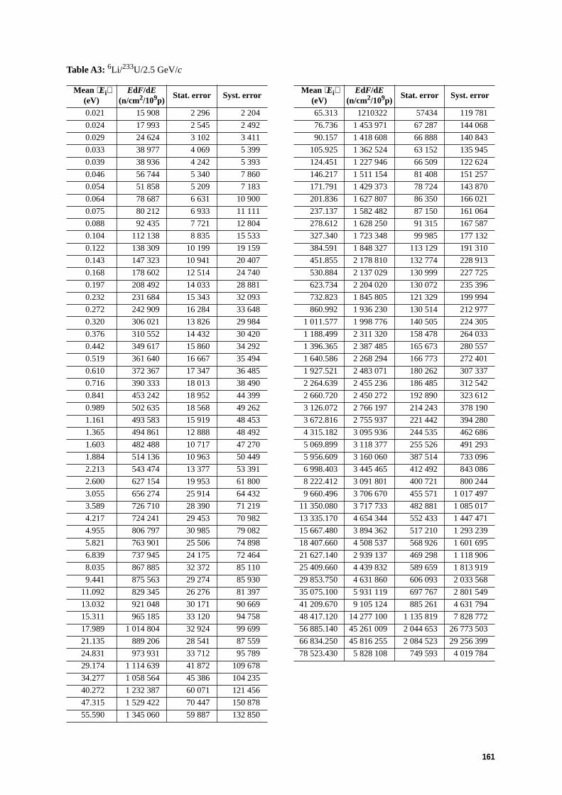
161

Table A3: 6Li/233U/2.5 GeV/c

Mean ⟨Ei⟩(eV)

EdF/dE(n/cm2/109p)

Stat. error Syst. error

0.021 15 908 2 296 2 204

0.024 17 993 2 545 2 492

0.029 24 624 3 102 3 411

0.033 38 977 4 069 5 399

0.039 38 936 4 242 5 393

0.046 56 744 5 340 7 860

0.054 51 858 5 209 7 183

0.064 78 687 6 631 10 900

0.075 80 212 6 933 11 111

0.088 92 435 7 721 12 804

0.104 112 138 8 835 15 533

0.122 138 309 10 199 19 159

0.143 147 323 10 941 20 407

0.168 178 602 12 514 24 740

0.197 208 492 14 033 28 881

0.232 231 684 15 343 32 093

0.272 242 909 16 284 33 648

0.320 306 021 13 826 29 984

0.376 310 552 14 432 30 420

0.442 349 617 15 860 34 292

0.519 361 640 16 667 35 494

0.610 372 367 17 347 36 485

0.716 390 333 18 013 38 490

0.841 453 242 18 952 44 399

0.989 502 635 18 568 49 262

1.161 493 583 15 919 48 453

1.365 494 861 12 888 48 492

1.603 482 488 10 717 47 270

1.884 514 136 10 963 50 449

2.213 543 474 13 377 53 391

2.600 627 154 19 953 61 800

3.055 656 274 25 914 64 432

3.589 726 710 28 390 71 219

4.217 724 241 29 453 70 982

4.955 806 797 30 985 79 082

5.821 763 901 25 506 74 898

6.839 737 945 24 175 72 464

8.035 867 885 32 372 85 110

9.441 875 563 29 274 85 930

11.092 829 345 26 276 81 397

13.032 921 048 30 171 90 669

15.311 965 185 33 120 94 758

17.989 1 014 804 32 924 99 699

21.135 889 206 28 541 87 559

24.831 973 931 33 712 95 789

29.174 1 114 639 41 872 109 678

34.277 1 058 564 45 386 104 235

40.272 1 232 387 60 071 121 456

47.315 1 529 422 70 447 150 878

55.590 1 345 060 59 887 132 850

Mean ⟨Ei⟩(eV)

EdF/dE(n/cm2/109p)

Stat. error Syst. error

65.313 1210322 57434 119 781

76.736 1 453 971 67 287 144 068

90.157 1 418 608 66 888 140 843

105.925 1 362 524 63 152 135 945

124.451 1 227 946 66 509 122 624

146.217 1 511 154 81 408 151 257

171.791 1 429 373 78 724 143 870

201.836 1 627 807 86 350 166 021

237.137 1 582 482 87 150 161 064

278.612 1 628 250 91 315 167 587

327.340 1 723 348 99 985 177 132

384.591 1 848 327 113 129 191 310

451.855 2 178 810 132 774 228 913

530.884 2 137 029 130 999 227 725

623.734 2 204 020 130 072 235 396

732.823 1 845 805 121 329 199 994

860.992 1 936 230 130 514 212 977

1 011.577 1 998 776 140 505 224 305

1 188.499 2 311 320 158 478 264 033

1 396.365 2 387 485 165 673 280 557

1 640.586 2 268 294 166 773 272 401

1 927.521 2 483 071 180 262 307 337

2 264.639 2 455 236 186 485 312 542

2 660.720 2 450 272 192 890 323 612

3 126.072 2 766 197 214 243 378 190

3 672.816 2 755 937 221 442 394 280

4 315.182 3 095 936 244 535 462 686

5 069.899 3 118 377 255 526 491 293

5 956.609 3 160 060 387 514 733 096

6 998.403 3 445 465 412 492 843 086

8 222.412 3 091 801 400 721 800 244

9 660.496 3 706 670 455 571 1 017 497

11 350.080 3 717 733 482 881 1 085 017

13 335.170 4 654 344 552 433 1 447 471

15 667.480 3 894 362 517 210 1 293 239

18 407.660 4 508 537 568 926 1 601 695

21 627.140 2 939 137 469 298 1 118 906

25 409.660 4 439 832 589 659 1 813 919

29 853.750 4 631 860 606 093 2 033 568

35 075.100 5 931 119 697 767 2 801 549

41 209.670 9 105 124 885 261 4 631 794

48 417.120 14 277 100 1 135 819 7 828 772

56 885.140 45 261 009 2 044 653 26 773 503

66 834.250 45 816 255 2 084 523 29 256 399

78 523.430 5 828 108 749 593 4 019 784

162

Table A4: 6Li/233U/3.5 GeV/c

Mean ⟨Ei⟩(eV)

EdF/dE(n/cm2/109p)

Stat. error Syst. error

0.075 136 821 13 481 18 952

0.088 147 269 14 511 20 400

0.104 189 792 17 113 26 290

0.122 193 421 17 959 26 793

0.143 261 752 21 715 36 258

0.168 273 486 23 056 37 883

0.197 330 851 26 321 45 830

0.232 387 450 29 543 53 670

0.272 390 250 30 732 54 059

0.320 391 459 31 883 54 226

0.376 495 989 37 146 68 707

0.442 530 785 39 748 73 528

0.519 514 308 40 412 71 246

0.610 639 911 46 296 88 647

0.716 709 795 49 304 98 329

0.841 703 736 48 107 97 492

0.989 790 865 47 406 109 565

1.161 793 205 41 031 109 892

1.365 683 367 30 834 94 678

1.603 810 821 28 306 112 340

1.884 751 001 26 947 104 056

2.213 921 449 35 404 127 679

2.600 1 003 056 51 234 138 995

3.055 1 053 106 66 747 145 941

3.589 1 100 545 71 161 152 527

4.217 1 164 793 76 101 161 447

4.955 1 290 617 79 843 178 907

5.821 1 076 456 61 718 149 239

6.839 1 209 259 62 936 167 677

8.035 1 406 360 83 962 195 042

9.441 1 156 057 68 458 160 363

11.092 1 274 007 66 292 176 768

13.032 1 323 097 73 489 183 633

15.311 1 374 192 80 492 190 790

17.989 1 418 413 79 236 197 009

21.135 1 347 106 71 421 187 194

24.831 1 453 772 83 838 202 129

29.174 1 519 187 99 654 211 362

34.277 1 733 481 118 260 241 361

40.272 1 888 361 151 566 263 162

47.315 1 938 158 161 616 270 386

55.590 1 919 220 145 759 268 075

65.313 2 061 837 152 886 288 412

76.736 2 300 584 172 370 322 354

90.157 2 050 328 163 891 287 859

105.925 2 017 214 156 183 283 868

124.451 2 368 271 187 930 334 174

146.218 2 437 672 210 622 345 059

171.791 2 295 428 203 646 326 127

201.836 2 154 312 203 343 307 399

Mean ⟨Ei⟩(eV)

EdF/dE(n/cm2/109p)

Stat. error Syst. error

237.137 2 369 321 217 854 339 778

278.612 2 460 551 229 689 354 924

327.340 2 280 036 233 981 331 117

384.591 2 756 006 281 549 403 385

451.855 2 745 673 304 728 405 525

530.884 3 279 609 352 961 552 844

623.734 2 695 023 293 074 407 059

732.823 2 715 284 300 159 415 781

860.992 3 005 634 331 130 467 497

1 011.577 3 070 210 355 556 486 105

1 188.499 3 056 556 371 178 493 772

1 396.366 3 084 099 384 940 509 627

1 640.586 3 221 901 405 771 546 065

1 927.522 3 045 267 407 881 530 904

2 264.640 2 995 790 419 121 538 855

2 660.721 4 076 129 508 180 758 821

3 126.073 3 383 133 482 334 653 933

3 672.817 3 637 157 519 923 732 330

4 315.182 3 858 717 557 878 811 939

5 069.900 4 370 950 619 146 964 219

5 956.610 3 494 666 569 171 810 721

6 998.404 3 356 627 568 649 821 348

8 222.412 3 822 169 622 289 989 283

9 660.496 2 886 462 561 498 792 347

11 350.080 3 954 690 695 597 1 154 173

13 335.180 4 563 132 763 981 1 419 105

15 667.480 3 873 365 720 433 1 286 267

18 407.670 4 333 018 778 993 1 539 341

21 627.140 4 400 745 802 051 1 675 327

25 409.670 4 831 128 859 098 1 973 784

29 853.750 5 840 420 950 571 2 564 174

35 075.110 4 162 665 816 448 1 966 224

41 209.680 4 905 666 907 566 2 495 524

48 417.130 4 258 432 866 393 2 335 089

56 885.140 4 116 317 861 217 2 434 949

66 834.250 4 170 700 878 419 2 663 240

78 523.440 5 345 556 1 002 671 3 686 956

92 256.960 5 612 317 1 042 980 4 183 208

163

Table A5: 3He/ionization/2.5 GeV/c

Ei/low(eV)

Mean ⟨Ei⟩(eV)

EdF/dE(n/cm2/109p)

Statisticalerror

Systematic error

59 500 84 250 4 769 990 585 185 858 598

109 000 133 750 5 513 695 766 895 992 465

158 500 183 250 7 339 415 1 079 366 1 321 095

208 000 232 750 6 917 651 1 154 588 1 176 001

257 500 282 250 10 017 312 1 627 418 1 702 943

307 000 331 750 6 167 753 1 283 921 1 048 518

356 500 381 250 9 621 671 1 816 459 1 635 684

406 000 430 750 8 704 919 1 812 074 1 392 787

455 500 480 250 8 429 564 1 884 908 1 348 730

505 000 529 750 10 091 790 2 221 605 1 614 686

554 500 579 250 7 095 639 1 910 559 1 135 302

604 000 628 750 5 036 533 1 670 429 805 845

653 500 678 250 5 692 027 1 887 832 910 724

703 000 727 750 12 173 780 3 046 648 1 947 805

752 500 777 250 2 858 499 1 457 554 457 360

802 000 851 500 2 481 939 1 043 202 397 110

901 000 950 500 2 492 927 1 142 402 398 868

1 000 000 1 081 154 2 233 198 938 652 357 312

1 162 308 1 256 634 2 491 258 1 047 119 398 601

1 350 960 1 460 596 959 095 684 930 153 455

1 570 232 1 697 662 1 814 799 1 063 375 290 368

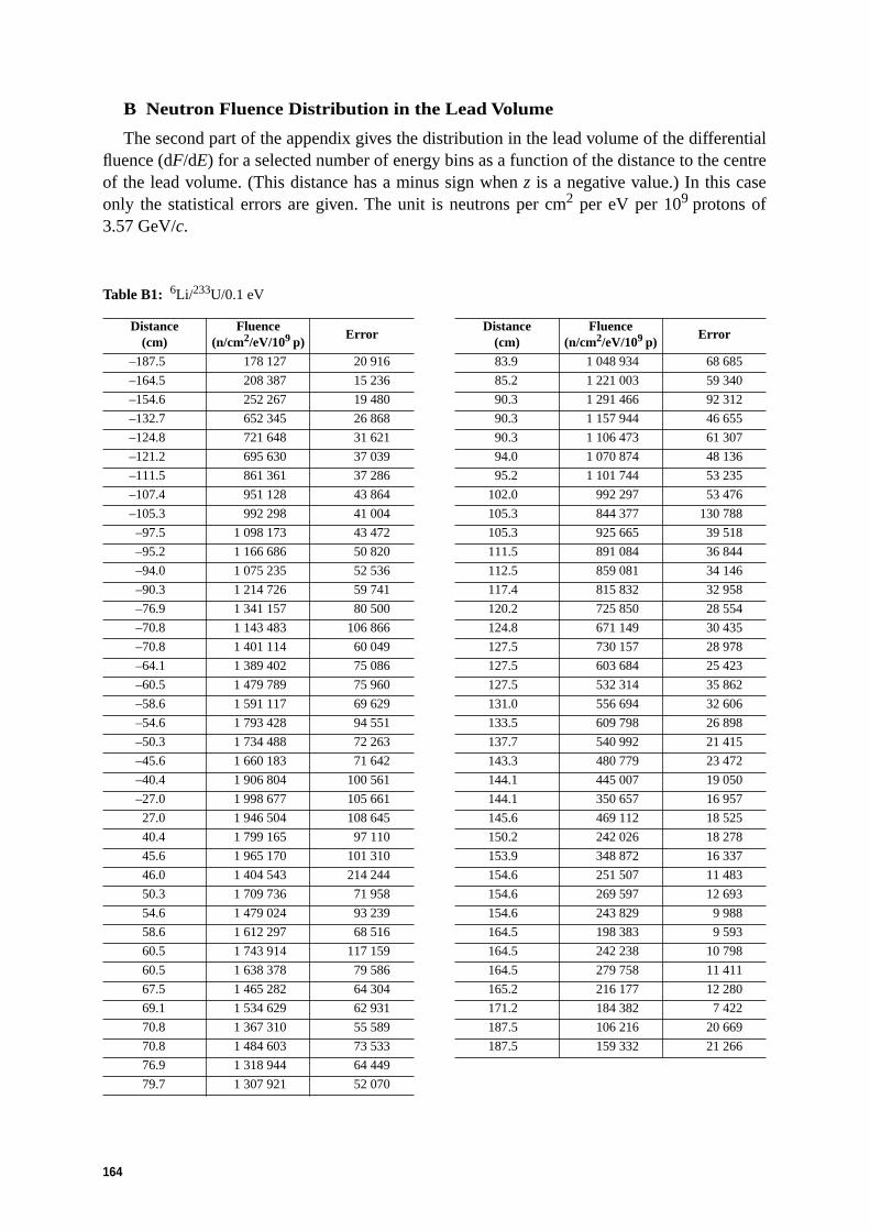
164

B Neutron Fluence Distribution in the Lead Volume

The second part of the appendix gives the distribution in the lead volume of the differentialfluence (dF/dE) for a selected number of energy bins as a function of the distance to the centreof the lead volume. (This distance has a minus sign when z is a negative value.) In this caseonly the statistical errors are given. The unit is neutrons per cm2 per eV per 109 protons of3.57 GeV/c.

Table B1: 6Li/233U/0.1 eV

Distance(cm)

Fluence(n/cm2/eV/109 p)

Error

–187.5 178 127 20 916

–164.5 208 387 15 236

–154.6 252 267 19 480

–132.7 652 345 26 868

–124.8 721 648 31 621

–121.2 695 630 37 039

–111.5 861 361 37 286

–107.4 951 128 43 864

–105.3 992 298 41 004

–97.5 1 098 173 43 472

–95.2 1 166 686 50 820

–94.0 1 075 235 52 536

–90.3 1 214 726 59 741

–76.9 1 341 157 80 500

–70.8 1 143 483 106 866

–70.8 1 401 114 60 049

–64.1 1 389 402 75 086

–60.5 1 479 789 75 960

–58.6 1 591 117 69 629

–54.6 1 793 428 94 551

–50.3 1 734 488 72 263

–45.6 1 660 183 71 642

–40.4 1 906 804 100 561

–27.0 1 998 677 105 661

27.0 1 946 504 108 645

40.4 1 799 165 97 110

45.6 1 965 170 101 310

46.0 1 404 543 214 244

50.3 1 709 736 71 958

54.6 1 479 024 93 239

58.6 1 612 297 68 516

60.5 1 743 914 117 159

60.5 1 638 378 79 586

67.5 1 465 282 64 304

69.1 1 534 629 62 931

70.8 1 367 310 55 589

70.8 1 484 603 73 533

76.9 1 318 944 64 449

79.7 1 307 921 52 070

Distance(cm)

Fluence(n/cm2/eV/109 p)

Error

83.9 1 048 934 68 685

85.2 1 221 003 59 340

90.3 1 291 466 92 312

90.3 1 157 944 46 655

90.3 1 106 473 61 307

94.0 1 070 874 48 136

95.2 1 101 744 53 235

102.0 992 297 53 476

105.3 844 377 130 788

105.3 925 665 39 518

111.5 891 084 36 844

112.5 859 081 34 146

117.4 815 832 32 958

120.2 725 850 28 554

124.8 671 149 30 435

127.5 730 157 28 978

127.5 603 684 25 423

127.5 532 314 35 862

131.0 556 694 32 606

133.5 609 798 26 898

137.7 540 992 21 415

143.3 480 779 23 472

144.1 445 007 19 050

144.1 350 657 16 957

145.6 469 112 18 525

150.2 242 026 18 278

153.9 348 872 16 337

154.6 251 507 11 483

154.6 269 597 12 693

154.6 243 829 9 988

164.5 198 383 9 593

164.5 242 238 10 798

164.5 279 758 11 411

165.2 216 177 12 280

171.2 184 382 7 422

187.5 106 216 20 669

187.5 159 332 21 266

165

Table B2: 6Li/233U/1.5 eV

Distance(cm)

Fluence(n/cm2/eV/109 p)

Error

–187.5 52 037 7 250

–164.5 60 333 2 796

–154.6 73 270 4 200

–150.2 75 772 4 035

–132.7 172 600 7 786

–124.8 208 772 9 666

–121.2 208 477 11 622

–111.5 262 848 19 126

–111.5 251 775 11 478

–107.4 285 943 13 805

–105.3 269 209 12 593

–97.5 291 771 13 215

–95.2 352 464 16 428

–94.0 340 796 16 835

–90.3 362 096 19 401

–90.3 366 357 18 540

–76.9 443 692 25 199

–70.8 374 540 49 984

–70.8 402 242 18 332

–67.5 481 558 31 378

–67.5 477 824 23 938

–64.1 445 496 23 782

–64.1 420 413 24 629

–60.5 475 073 24 555

–58.6 489 428 23 622

–54.6 479 350 36 273

–54.6 540 276 31 094

–50.3 524 329 24 304

–50.3 515 078 23 643

–45.6 538 414 23 636

–40.4 573 929 31 042

–27.0 563 951 56 170

–27.0 610 220 34 302

27.0 597 918 34 339

40.4 546 907 33 215

45.6 536 203 26 304

46.0 435 567 49 354

50.3 498 337 22 665

54.6 517 116 29 952

58.6 455 746 21 531

60.5 491 059 25 864

60.5 474 549 25 428

60.5 484 480 25 025

67.5 415 905 38 030

67.5 433 361 20 431

69.1 422 865 20 274

70.8 388 025 17 357

70.8 434 043 22 920

70.8 412 295 27 045

76.9 364 314 37 569

76.9 395 237 20 274

Distance(cm)

Fluence(n/cm2/eV/109 p)

Error

79.7 354 786 16 006

81.1 378 500 37 086

83.9 351 309 22 740

85.2 374 363 19 518

90.3 324 092 19 276

90.3 308 537 13 998

90.3 341 238 19 812

90.3 351 774 21 177

92.8 368 103 19 033

94.0 304 353 14 503

95.2 321 900 16 641

102.0 257 844 21 189

102.0 283 505 16 470

105.3 271 252 22 573

105.3 268 307 12 532

105.3 252 442 12 043

111.5 242 475 11 123

111.5 246 286 12 376

112.5 218 185 9 735

117.4 216 957 18 756

117.4 213 167 24 040

117.4 227 283 10 334

120.2 186 689 8 444

124.8 191 253 9 300

124.8 198 983 9 080

124.8 200 761 8 998

127.5 186 511 8 635

127.5 166 697 7 994

127.5 161 090 11 119

127.5 155 814 12 734

131.0 150 208 9 615

133.5 170 289 8 173

137.7 134 541 6 071

143.3 132 267 9 824

143.3 138 269 6 995

144.1 121 826 5 621

144.1 103 701 5 192

145.6 116 794 5 352

150.2 69 495 8 780

150.2 73 972 4 350

153.9 96 561 5 095

154.6 71 825 3 481

154.6 71 305 3 458

154.6 68 455 3 110

164.5 57 475 2 947

164.5 58 911 2 877

164.5 69 183 3 199

165.2 61 544 3 585

171.2 47 362 2 193

187.5 29 628 1 587

187.5 34 947 1 689

166

Table B3: 6Li/233U/5 eV

Distance(cm)

Fluence(n/cm2/eV/109 p)

Error

–187.5 19 654 3 775

–164.5 23 255 1 093

–154.6 28 522 1 666

–150.2 29 988 1 721

–132.7 66 240 3 049

–124.8 81 051 3 790

–121.2 82 117 4 661

–111.5 105 704 9 652

–111.5 97 672 4 424

–107.4 110 736 5 439

–105.3 104 929 4 826

–97.5 112 948 5 058

–95.2 139 589 6 534

–94.0 135 880 7 070

–90.3 144 366 7 872

–90.3 148 753 8 028

–76.9 173 919 10 862

–70.8 151 538 25 055

–70.8 152 228 7 128

–67.5 183 371 14 961

–67.5 192 210 11 922

–64.1 178 006 10 140

–64.1 171 565 10 552

–60.5 190 845 10 178

–58.6 198 896 9 008

–54.6 198 543 16 385

–54.6 221 945 12 552

–50.3 207 810 10 763

–50.3 208 064 9 314

–45.6 214 427 9 596

–40.4 234 634 13 543

–27.0 219 351 29 333

–27.0 246 342 14 200

27.0 246 591 15 097

40.4 224 161 13 512

45.6 214 558 11 421

46.0 178 277 34 321

50.3 200 567 9 076

54.6 204 048 12 301

58.6 187 469 8 673

60.5 195 491 12 339

60.5 190 137 10 444

60.5 193 141 10 628

67.5 159 567 19 067

67.5 171 050 8 002

69.1 172 297 7 824

70.8 151 338 6 762

70.8 171 693 9 521

70.8 164 591 11 145

76.9 173 333 20 852

76.9 155 287 8 340

Distance(cm)

Fluence(n/cm2/eV/109 p)

Error

79.7 139 681 6 195

81.1 149 211 15 392

83.9 139 398 9 484

85.2 147 546 7 751

90.3 127 203 9 142

90.3 120 764 5 280

90.3 135 269 7 885

90.3 135 597 8 838

92.8 144 734 8 759

94.0 119 849 5 903

95.2 124 716 6 937

102.0 103 624 10 581

102.0 109 857 7 022

105.3 104 741 10 277

105.3 104 519 4 950

105.3 97 749 4 845

111.5 93 341 4 274

111.5 94 634 4 839

112.5 82 193 3 672

117.4 85 547 11 095

117.4 85 349 14 371

117.4 88 025 3 608

120.2 70 531 3 157

124.8 73 397 3 470

124.8 78 090 3 603

124.8 78 385 3 459

127.5 69 544 3 096

127.5 64 191 2 978

127.5 60 962 4 475

127.5 59 521 4 677

131.0 57 224 3 867

133.5 64 979 3 196

137.7 50 557 2 232

143.3 47 420 4 926

143.3 52 529 2 765

144.1 46 303 2 133

144.1 39 465 2 013

145.6 43 679 1 946

150.2 26 193 3 588

150.2 27 994 1 728

153.9 36 002 1 892

154.6 27 536 1 363

154.6 26 758 1 340

154.6 26 318 1 193

164.5 21 902 1 139

164.5 21 728 1 135

164.5 25 603 1 154

165.2 23 063 1 463

171.2 17 841 819

187.5 11 053 672

187.5 12 680 641

167

Table B4: 6Li/233U/10 eV

Distance(cm)

Fluence(n/cm2/eV/109 p)

Error

–187.5 10 787 2 087

–164.5 12 973 682

–154.6 16 029 1 040

–150.2 16 823 1 044

–132.7 37 060 1 781

–124.8 45 469 2 252

–121.2 46 469 2 928

–111.5 59 793 4 664

–111.5 54 722 2 772

–107.4 61 839 3 443

–105.3 59 306 2 869

–97.5 63 596 2 944

–95.2 79 278 4 101

–94.0 77 315 4 362

–90.3 82 491 5 048

–90.3 84 399 5 004

–76.9 97 383 6 723

–70.8 87 004 7 565

–70.8 83 784 4 240

–67.5 103 674 8 171

–67.5 109 837 6 506

–64.1 101 372 6 318

–64.1 98 073 6 950

–60.5 109 123 6 420

–58.6 115 080 6 008

–54.6 114 736 9 192

–54.6 129 676 8 399

–50.3 119 080 6 141

–50.3 120 122 5 597

–45.6 121 708 5 960

–40.4 136 590 8 962

–27.0 121 178 16 016

–27.0 141 880 9 266

27.0 144 317 8 974

40.4 130 661 8 990

45.6 123 695 6 426

46.0 103 661 9 005

50.3 115 618 5 571

54.6 114 399 8 418

58.6 110 128 5 254

60.5 112 016 6 757

60.5 109 275 6 325

60.5 109 903 6 871

67.5 91 304 10 339

67.5 97 038 4 866

69.1 100 656 4 916

70.8 85 314 4 015

70.8 97 644 5 502

70.8 92 960 6 999

76.9 93 183 12 350

76.9 87 705 5 109

Distance(cm)

Fluence(n/cm2/eV/109 p)

Error

79.7 79 562 3 735

81.1 84 859 9 087

83.9 78 723 6 080

85.2 83 401 5 014

90.3 72 673 5 372

90.3 68 564 3 178

90.3 76 771 5 176

90.3 75 967 5 568

92.8 81 769 4 651

94.0 68 056 3 515

95.2 69 807 4 261

102.0 58 161 5 694

102.0 61 592 4 372

105.3 58 092 5 792

105.3 58 780 2 908

105.3 54 528 2 858

111.5 52 244 2 581

111.5 52 313 2 905

112.5 45 462 2 131

117.4 47 536 5 508

117.4 47 586 6 566

117.4 49 418 2 269

120.2 39 064 1 821

124.8 40 854 2 149

124.8 43 521 2 176

124.8 43 647 2 088

127.5 38 148 1 714

127.5 35 901 1 832

127.5 33 429 2 764

127.5 32 990 3 382

131.0 31 792 2 436

133.5 36 060 1 891

137.7 27 950 1 310

143.3 25 418 2 519

143.3 28 993 1 676

144.1 25 652 1 269

144.1 21 769 1 220

145.6 24 058 1 119

150.2 14 371 1 146

150.2 15 479 1 026

153.9 19 639 1 159

154.6 15 312 838

154.6 14 715 845

154.6 14 684 697

164.5 12 111 703

164.5 11 859 672

164.5 13 995 670

165.2 12 605 915

171.2 9 860 472

187.5 6 029 409

187.5 6 884 386

168

Table B5: 6Li/233U/18 eV

Distance(cm)

Fluence(n/cm2/eV/109 p)

Error

–187.5 6 356 961

–164.5 7 770 395

–154.6 9 671 648

–150.2 10 087 658

–132.7 22 305 1 000

–124.8 27 386 1 314

–121.2 28 211 1 707

–111.5 36 102 2 540

–111.5 32 910 1 560

–107.4 37 046 1 964

–105.3 36 039 1 666

–97.5 38 516 1 628

–95.2 48 296 2 394

–94.0 47 140 2 562

–90.3 50 574 3 085

–90.3 51 043 3 071

–76.9 58 376 4 215

–70.8 53 488 4 327

–70.8 49 520 2 336

–67.5 63 378 4 274

–67.5 67 202 3 622

–64.1 61 844 3 630

–64.1 59 825 4 102

–60.5 66 840 3 822

–58.6 71 393 3 463

–54.6 70 743 5 261

–54.6 81 271 5 004

–50.3 73 381 3 678

–50.3 74 414 3 313

–45.6 73 987 3 483

–40.4 85 294 5 308

–27.0 71 502 7 595

–27.0 87 630 5 685

27.0 90 560 5 954

40.4 81 680 5 539

45.6 76 659 3 624

46.0 64 615 5 776

50.3 71 544 3 376

54.6 68 582 5 240

58.6 69 490 3 165

60.5 68 951 3 730

60.5 67 424 3 927

60.5 67 016 4 148

67.5 56 597 6 311

67.5 59 077 2 863

69.1 63 197 2 896

70.8 51 658 2 209

70.8 59 608 3 596

70.8 56 113 4 570

76.9 54 894 6 303

76.9 53 143 3 046

Distance(cm)

Fluence(n/cm2/eV/109 p)

Error

79.7 48 723 2 063

81.1 51 845 5 663

83.9 47 582 3 704

85.2 50 552 2 925

90.3 44 713 2 580

90.3 41 868 1 840

90.3 46 715 3 037

90.3 45 754 3 523

92.8 49 557 2 689

94.0 41 508 2 079

95.2 41 942 2 583

102.0 34 765 3 364

102.0 37 086 2 552

105.3 34 516 3 363

105.3 35 491 1 705

105.3 32 622 1 659

111.5 31 437 1 499

111.5 30 984 1 709

112.5 27 074 1 159

117.4 28 172 2 939

117.4 28 223 3 654

117.4 29 812 1 318

120.2 23 289 1 011

124.8 24 423 1 257

124.8 25 922 1 190

124.8 25 999 1 173

127.5 22 529 1 026

127.5 21 580 1 046

127.5 19 663 1 822

127.5 19 634 1 954

131.0 18 993 1 550

133.5 21 502 1 090

137.7 16 645 707

143.3 14 701 1 414

143.3 17 184 973

144.1 15 277 719

144.1 12 887 753

145.6 14 273 620

150.2 8 467 671

150.2 9 204 676

153.9 11 513 712

154.6 9 145 491

154.6 8 705 484

154.6 8 803 403

164.5 7 190 409

164.5 6 976 379

164.5 8 241 384

165.2 7 400 506

171.2 5 866 268

187.5 3 533 242

187.5 4 036 219

169

Table B6: 6Li/233U/100 eV

Distance(cm)

Fluence(n/cm2/eV/109 p)

Error

–187.5 1 257 232

–164.5 1 637 101

–154.6 2 095 181

–150.2 2 100 180

–132.7 4 818 261

–124.8 5 894 351

–121.2 6 242 564

–111.5 7 688 951

–111.5 7 037 439

–107.4 7 789 545

–105.3 8 061 442

–97.5 8 519 438

–95.2 10 821 676

–94.0 10 558 712

–90.3 11 620 901

–90.3 10 888 845

–76.9 12 217 1 184

–70.8 12 334 1 316

–70.8 9 923 631

–67.5 14 786 1 543

–67.5 15 212 1 217

–64.1 13 871 1 084

–64.1 13 237 1 239

–60.5 15 221 1 191

–58.6 17 121 1 055

–54.6 16 296 2 031

–54.6 20 293 1 740

–50.3 17 330 1 135

–50.3 17 794 1 034

–45.6 16 357 978

–40.4 21 007 1 554

–27.0 13 977 3 914

40.4 20 184 2 036

45.6 18 474 1 227

46.0 15 769 1 721

50.3 17 059 1 049

54.6 14 299 1 467

58.6 17 890 1 071

60.5 16 155 1 277

60.5 15 908 1 284

60.5 15 019 1 125

67.5 14 015 2 598

67.5 13 224 845

69.1 15 993 944

70.8 11 361 608

70.8 13 493 1 001

70.8 11 989 1 244

76.9 11 636 2 673

76.9 11 672 874

79.7 11 225 600

Distance(cm)

Fluence(n/cm2/eV/109 p)

Error

81.1 11 806 2 153

83.9 10 268 1 143

85.2 11 098 820

90.3 10 546 849

90.3 9 553 510

90.3 10 405 903

90.3 9 890 1 090

92.8 10 890 838

94.0 9 383 613

95.2 8 936 733

102.0 7 069 1 136

102.0 7 980 774

105.3 6 998 1 132

105.3 7 709 474

105.3 6 816 451

111.5 6 772 411

111.5 6 210 471

112.5 5 635 298

117.4 5 572 1 058

117.4 5 549 1 456

117.4 6 473 332

120.2 4 862 256

124.8 5 114 327

124.8 5 263 324

124.8 5 297 303

127.5 4 539 252

127.5 4 624 270

127.5 3 854 472

127.5 4 039 582

131.0 3 982 453

133.5 4 465 298

137.7 3 469 181

143.3 2 756 428

143.3 3 480 266

144.1 3 162 185

144.1 2 592 202

145.6 2 932 160

150.2 1 676 185

150.2 1 897 197

153.9 2 242 190

154.6 1 907 138

154.6 1 761 132

154.6 1 865 108

164.5 1 465 117

164.5 1 390 96

164.5 1 646 97

165.2 1 446 149

171.2 1 215 73

187.5 687 63

187.5 800 57

170

Table B7: 6Li/233U/480 eV

Distance(cm)

Fluence(n/cm2/eV/109 p)

Error

–187.5 262 40

–164.5 372 31

–154.6 493 57

–150.2 464 57

–132.7 1 136 71

–124.8 1 377 92

–121.2 1 509 149

–111.5 1 745 266

–111.5 1 628 114

–107.4 1 760 149

–105.3 1 988 126

–97.5 2 072 115

–95.2 2 660 196

–94.0 2 587 219

–90.3 2 955 277

–90.3 2 468 268

–76.9 2 729 305

–70.8 3 136 388

–70.8 2 108 685

–67.5 3 912 532

–67.5 3 773 381

–64.1 3 403 307

–64.1 3 158 346

–60.5 3 810 307

–54.6 4 100 658

–50.3 4 597 330

–50.3 4 773 347

45.6 5 030 390

46.0 4 336 540

50.3 4 563 354

58.6 5 307 344

60.5 4 229 393

60.5 4 197 360

60.5 3 683 328

67.5 4 033 862

69.1 4 644 300

70.8 2 733 183

70.8 3 368 315

70.8 2 742 386

76.9 2 802 784

76.9 2 795 265

79.7 2 879 172

81.1 2 976 596

83.9 2 387 292

85.2 2 653 255

90.3 2 803 310

90.3 2 422 137

90.3 2 535 264

90.3 2 330 338

92.8 2 609 239

Distance(cm)

Fluence(n/cm2/eV/109 p)

Error

94.0 2 341 179

95.2 2 058 203

102.0 1 500 322

102.0 1 864 213

105.3 1 501 378

105.3 1 822 125

105.3 1 526 134

111.5 1 589 107

111.5 1 312 142

112.5 1 267 75

117.4 1 144 309

117.4 1 123 377

117.4 1 532 82

120.2 1 097 66

124.8 1 153 90

124.8 1 124 80

124.8 1 140 76

127.5 978 67

127.5 1 077 82

127.5 793 136

127.5 889 203

131.0 902 124

133.5 996 83

137.7 783 45

143.3 542 139

143.3 750 74

144.1 703 49

144.1 553 49

145.6 649 41

150.2 351 55

150.2 420 59

153.9 460 50

154.6 427 36

154.6 381 33

154.6 427 28

164.5 318 37

164.5 296 28

164.5 351 24

165.2 297 38

171.2 271 18

187.5 141 17

187.5 170 15

171

Table B8: 6Li/233U/1000 eV

Distance(cm)

Fluence(n/cm2/eV/109 p)

Error

–187.5 122 24

–164.5 182 19

–154.6 247 31

–150.2 223 33

–132.7 571 46

–124.8 687 63

–121.2 769 89

–111.5 853 163

–111.5 808 72

–107.4 860 90

–105.3 1 027 83

–97.5 1 061 68

–95.2 1 369 111

–94.0 1 329 128

–90.3 1 554 164

–90.3 1 205 161

–76.9 1 323 192

–70.8 1 647 250

–67.5 2 115 311

–67.5 1 952 203

–64.1 1 749 182

–54.6 2 137 405

–50.3 2 484 194

–50.3 2 594 214

–45.6 1 997 192

45.6 2 761 225

46.0 2 392 336

50.3 2 476 181

58.6 3 072 198

60.5 2 266 232

67.5 2 299 461

69.1 2 653 189

70.8 1 389 110

70.8 1 751 185

70.8 1 348 198

76.9 1 436 475

76.9 1 416 149

79.7 1 524 101

81.1 1 557 367

85.2 1 342 156

90.3 1 517 194

90.3 1 297 172

90.3 1 170 200

92.8 1 322 148

94.0 1 217 124

95.2 1 018 127

102.0 930 124

105.3 916 85

105.3 741 88

111.5 795 73

Distance(cm)

Fluence(n/cm2/eV/109 p)

Error

111.5 615 82

112.5 619 46

117.4 525 162

117.4 511 214

117.4 771 51

120.2 537 41

124.8 563 58

124.8 530 50

124.8 540 46

127.5 536 51

127.5 427 102

131.0 442 74

133.5 483 53

137.7 383 27

143.3 356 43

144.1 341 31

144.1 261 30

145.6 314 27

150.2 163 32

150.2 203 36

153.9 212 34

154.6 208 24

154.6 181 20

154.6 211 18

164.5 152 21

164.5 139 17

164.5 166 17

165.2 137 25

171.2 132 12

187.5 80 10

172

Table B9: 3He/scintillation/1.5 eV

Table B10: 3He/scintillation/5 eV

Table B11: 3He/scintillation/10 eV

DistanceFluence

(n/cm2/eV/109 p)Error

16.8 665 235 9 979

40.4 593 298 9 474

45.6 602 514 9 483

69.1 387 449 7 658

81.1 420 921 7 966

98.6 331 789 7 105

105.3 275 497 6 362

113.5 218 988 5 755

124.8 207 045 5 607

153.9 115 093 4 100

DistanceFluence

(n/cm2/eV/109 p)Error

16.8 284 113 4 660

40.4 245 043 4 334

45.6 266 956 4 501

69.1 168 293 3 576

81.1 180 439 3 725

98.6 130 339 3 166

105.3 119 252 3 013

113.5 93 661 2 677

124.8 88 648 2 604

153.9 42 240 1 747

DistanceFluence

(n/cm2/eV/109 p)Error

16.8 167 763 3 135

40.4 143 894 2 910

45.6 157 657 3 064

69.1 96 559 2 392

81.1 107 418 2 504

98.6 75 270 2 105

105.3 67 229 2 005

113.5 54 325 1 795

124.8 49 735 1 721

153.9 24 108 1 196

Table B12: 3He/scintillation/18 eV

Table B13: 3He/scintillation/100 eV

Table B14: 3He/scintillation/480 eV

DistanceFluence

(n/cm2/eV/109 p)Error

16.8 10 5971 2 071

40.4 9 0614 1 921

45.6 10 0489 2 019

69.1 59 547 1 556

81.1 66 724 1 647

98.6 47 353 1 383

105.3 41 776 1 301

113.5 32 850 1 151

124.8 30 290 1 107

153.9 14 574 755

DistanceFluence

(n/cm2/eV/109 p)Error

16.8 26 393 656

40.4 21 271 588

45.6 24 639 634

69.1 14 014 478

81.1 15 459 502

98.6 10 163 407

105.3 9 156 387

113.5 7 627 353

124.8 6 354 322

153.9 2 970 220

DistanceFluence

(n/cm2/eV/109 p)Error

16.8 6 932 247

40.4 5 332 217

45.6 6 363 240

69.1 3 500 180

81.1 3 989 188

98.6 2 635 154

105.3 2 244 140

113.5 1 833 125

124.8 1 480 113

153.9 755 79

173

Table B15: 3He/scintillation/1000 eV

Table B16: 3He/scintillation/10 000 eV

Table B17: 3He/scintillation/50 000 eV

DistanceFluence

(n/cm2/eV/109 p)Error

16.8 3 746 144

40.4 2 736 124

45.6 3 440 139

69.1 1 835 102

81.1 2 070 108

98.6 1 359 87

105.3 1 092 78

113.5 938 72

124.8 705 61

153.9 316 43

DistanceFluence

(n/cm2/eV/109 p)Error

16.8 496 32

40.4 399 28

45.6 603 36

69.1 313 25

81.1 316 26

98.6 200 21

105.3 148 16

113.5 128 16

124.8 82 9

153.9 47 9

DistanceFluence

(n/cm2/eV/109 p)Error

81.1 81 10

98.6 61 8

105.3 27 4

113.5 30 6

124.8 16 5

153.9 9 3

174

Table B18: Triple-foil activation data

Distance(cm)

Indium(n/cm2/eVper 109 p)

Error-indiumGold

(n/cm2/eV per 109 p)

Error-goldTungsten

(n/cm2/eV per 109 p)

Error-tungsten

–127.5 – – – – 30 992 3 808

–127.5 – – 71 100 9 609 30 992 3 808

–127.5 202 268 38 955 – – – –

–90.3 – – – – 64 198 7 404

–90.3 – – 138 969 18 979 59 771 7 438

–90.3 396 527 49 671 – – – –

–27 – – – – 103 308 13 138

–27 – – 216 533 31 315 94 453 11 985

–27 552 350 78 228 – – – –

–27 555 531 78 758 – – – –

16.8 – – 252 084 31 803 109 949 13 241

16.8 – – – – 114 377 14 025

16.8 583 130 79 118 – – – –

60.5 – – – – 80 433 9 976

60.5 – – 219 765 27 277 79 695 9 917

60.5 426 600 61 575 – – – –

67.5 – – – – 94 453 10 765

69.1 – – – – 67 150 8 940

69.1 – – 161 592 22 852 75 267 9 128

69.1 386 280 54 658 – – – –

70.8 – – – – 63 461 8 182

70.8 – – 171 288 23 548 74 529 9 067

70.8 424 716 56 162 – – – –

70.8 515 799 63 998 – – – –

105.3 – – – – 45 751 5 444

105.3 – – – – 48 702 6 110

105.3 – – 100 187 13 942 42 061 5 138

105.3 278 276 36 206 – – – –

153.9 – – – – 15 496 2 140

153.9 – – 42 014 5 300 14 020 2 035

153.9 112 991 14 687 – – – –

153.9 97 836 12 999 – – – –