TECHNICAL REPORT

Respiratory and Immunologic Evaluation of Isocyanate Exposure in a New Manufacturing Plant

U.S. DEPARTMENT OF HEAL TH AND HUMAN SERVICES Public Health Service Centers for Disease Control National Institute for Occupational Safety and Health

Respiratory and Immunologic Evaluation of Isocyanate Exposure in a New

Manufacturing Plant

Hans Weill, M.D. Brian Butcher, Ph.D.

Venkatram Dharmarajan, Ph.D. Henry Glindmeyer, D.Eng.

Robert Jones, M.D. Jean Carr, M.S.H. Carol O'Neil, M.S.

John Salvaggio, M.D. Tulane University School of Medicine

New Orleans, Louisiana

NIOSH Contract No. 210-75-0006

U.S . DEPARTMENT OF HEALTH AND HUMAN SERVICES Public Health Service

Centers for Disease Control National Institute for Occupational Safety and Health

Division of Respiratory Disease Studies Morgantown, West Virginia

June 1981 Few •ale by the Superintendent of Document"•, U .S. Government

Printing_ Office , Washiniiton, D .C. 20402

DISCLAIMER

Mention of company names or products does not constitute endorsement by the National Institute for Occupational Safety and Health.

NIOSH Project Officer: James A. Merchant, M.D., Dr. P.H. Principal Investigator: Hans Weill, M.D.

DHHS (NIOSH) Publication No. 81-125

if

ABSTRACT

In April, 1973, pre-exposure (baseline) information was obtained on 168 workers who were to begin manufacturing toluene diisocyanate (TDI) in four months. None of these workers had prior exposure to TDI. Subsequent follow-up in this longitudinal investigation was five and one-half years in length, during which time eight additional visits were made to· the manufac­turing site. At each of visits 2, 3, 4 and 5, approximately 25 participants were added to the study population, bringing the total size of the study population to 277 . The added participants had no more than 11 months of TDI exposure prior to inclusion in the study .

Exposure to TDI vapor was determined by personal monitors utilizing the paper tape stain method for continuous 8-hour measurement . The approxi­mately 2,000 personal samples collected had median 8- hour time- weighted aver­ages of .002 ppm. The 25th and 75th percentiles were .0011 and . 0036 respect­ively. Percentage of time above . 02 ppm, the current threshold limit value , averaged 3% in these personal samples . All members of the study population had some degree of TDI exposure, which depended on both job and location . No systematic trends in exposure were observed over the course of the study .

Detailed job histories allowed for the construction of cumulative exposure as a product of concentration and time. Cumulative exposure was used to define two exposure categories (division point= . 0682 ppm-months) with the low category chosen to represent the exposure received by a worker who spent the full follow-up period in a group of jobs (median 8- hour time­weighted average~ .0011 ppm) with the lowest TDI concentration.

Pulmonary function annual changes for spirometric measurements, lung volumes and diffusing capacities were computed for each participant as the slope of the least squares straight line using time as the independent variable .

The average annual decline of FEV1 was 24 ml per year , comparable to that expected on the basis of cross sectional studies of "normal" populations . Average annual declines of FEF25_75 and FEF50 were 93 and 110 ml, larger than expected on the bas.is of cross sectional data. Average annual declines for single breath. carbon monoxide diffusing capacity and the diffusion constant (K) were also larger than expected on the basis of cross sectional results .

After controlling for pack years of smoking and atopic status, FEV1 , FEV% and FEF2s- 75 annual declines were significantly related to the TDI

·exposure categories . Lung volume and diffusing capacity annual change was not related to TDI exposure.

iii

The effect of TDI exposure on FEV1

annual change was manifest primarily in those who never smoked cigarettes; its effect in smokers may be masked by smoking. In the never smokers·, there was a 38 ml per year (p = .001) difference between the low and liigh exposure categories. Among current smokers there was· no observed effect of TDT. In the low exposure category, there was a 27 ml per year (p = • 004) difference oetween never and current cigarette smokers-. This· difference is comparable to the effect of TDI in the never smokers-. Current smokers averaged 18 pack years of smoking. Never smokers in the low exposure group had an average annual increase in FEV1 of 1 ml per year.

TDI exposure as determined by cumulative dose and peak exposure as measured by time spent above 0.02 ppm correlated equally well with annual change in pulmonary function.

Clinically important bronchial hypersensitivity to TD!' developed in 4.3% of the study population. A number of these workers were shown to develop bronchoconstriction in the laooratory following inhalation challenge using a maximum concentration of 0.02 ppm TDT. Half of the TDI reactors had been exposed to high_ levels during a spill or equipment -mal:Eunction. 75% of the reactors b.ecame symptomatic wi.thin seven -months of firs·t exposure to TDI. Some TDI reactors have failed to attain pre-exposure or pre ... sensitization values of FEV1 or FEF25-75 despite transfer to other areas of the chemical complex. Neither atopy nor smoking served to identify persons at higher risk of developing TDI reactivity.

TDI at certain concentrations acts as a partial agonist on lymphocytes to stimulate cyclic adenosine monophosphate (AMP) levels. At lower concen­trations, it can block cyclic AMP stimulation by isoproterenol and prosta­glandin E1 but not histamine. Lymphocytes of TDT sensitive individuals have decreased ability to respond to cyclic AMP stimuli such as beta agonists, isoproterenol, prostaglandin E1 and TDT.

RAST with p-tolyl isocyanate conjugated to human serum albumin only detects tolyl specificlgE antibodies in the serum of 15-18% of subjects proven by provocative inhalation challenge to be TDI reactive. This demon­strates that the presence of tolyl specific serum tgE antibodies cannot be used to diagnose clinical sensitivity to TDI.

All other humoral or cellular indicators of immunologic sensitization were non-revealing.

iv

I.

II.

III.

IV.

v.

TABLE OF CONTENTS

Introduction

Study Design and Protocols

TD! Exposure Indices

A.

B.

C.

Cumulative Exposures

Time Above • 02 PPM

Assignment of Exposure Indices for Correlation Studies

Longitudinal Results and Analysis

A.

B.

c.

D.

E.

Introduction

Spirometry Results

Diffusion and Long Volume

Respiratory Symptoms

Immunology

F. Detail~d Analysis of FEV1 Slope

TD! Reactors

A.

B.

c.

D.

E.

F.

G.

Clinical and Epidemiologic Features

Immunologic Findings

Provocative Inhalation Challenge with TDI

Challenge Testing with Methacholine Chloride (Mecholyl)

Study of the Effect of Pretreatment with Disodium Cromoglycate

Lymphocyte Transformation and Leukocyte Histamine Release

Lymphocyte cAMP Dose Response Studies

V

Page Number

1

3

8

9

11

11

12

12

15

20

20

23

23

29

29

30

31

31

32

32

32

v.

VI.

H.

I.

J.

K.

L.

TABLE OF CONTENTS (Continued)

Plasma Histamine Levels

Determination of Serum Complement and Split Products of Complement

Loss of TD! and Methacholine Reactivity after Removal from Isocyanate Exposure

Concurrent Development of Food Allergy and Isocyanate Reactivity

Tolyl-specific IgE Antibodies in Serum of TD! Reactive Individuals

Conclusions

Appendix 1 - Environmental Characterization

Appendix 2 - Statistical Considerations

Appendix 3 - Interview Forms, Symptom Criteria

References

Tables

Figures

Reprints

and Editorial Programs

vi

Page Number

33

33

34

34

34

36

39

48

59

94

98

130

152

I. INTRODUCTION

The construction of a new plant in Southwestern Louisiana for production of toluene diisocyanate (TD!) with start of operation late in 1973 led to a proposal by the National Institute of Occupational Safety and Health (NIOSH) to the investigators for a longitudinal study of respir­atory health of the workers who would be exposed to TDI. The ability to begin the study prior to the start of TDI production presented the unique opportunity of obtaining pre-exposure biologic data on the study popula­tion. The proposed investigation had the full agreement and cooperation of the major chemical company operating this plant and its labor representa­tives.

It has been known for two decades that reversible airways obstruc­tion develops in a small proportion of workers exposed to isocyanate vapors, either during manufacture or application processes. In addition to the recognition of the risk for developing this form of occupational asthma, there had been a suggestion that chronic progressive fixed airways obstruc­tion was detected in an exposed population and was not related to "sensitiv­ity", but rather was a general effect of TD! exposure.

This multi-disciplinary investigation addressed the following scientific questions:

(1) What are the characteristics of plant airborne TDI concen­trations, particularly in terms of average exposures, as well as variation in short term concentrations (peaks)? This was first assessed by area moni­toring using a physico-chemical method for continuous monitoring developed in the United Kingdom and introduced into this investigation by the principal investigator resulting in its first research or other application in the United States. During the course of the contract, personal sampling for con­tinuous airborne concentrations of TDI vapor was similarly initiated and formed the basis for the comprehensive personal exposure profiles in these manufacturing workers detailed in this report.

(2) What proportion of exposed workers become reactive to TD! vapor following exposure, what are the temporal relationships between initial exposure and such reactivity, and what are the clinical manifestations in the reactive group?

(3) Are there host factors which will serve to identify those ~ndividuals who are susceptible to TDI exposure and develop the clinical picture of occupational asthma as the result of such exposure?

1

(4) Can the phy~iologic consequences (bronchoconstriction) of e...xposure in susceptible workers be reproduced in the laocratc~J by brcnchc­provocation; and what are the physiologic, immunologic and exposure charac­teristics of such a reproduced bronchoconstrictor response?

(5) What is the mechanism of TD! induced asthma? Is it immuno­logic or non-i1I1TJ1unologic?

(6) Is there a generalized adverse effect on respiratory function in the exposed working popuiation, and if so, what are its determinants (e.g., host factors, level of exposure)?

(7) Is the airways obstruction which results from development of TD! reactivity reversible in all instances, or are there permanent residual effects which are measurable by follow-up serial ventilatory function studies? If permanent changes occur in some reactive individuals, what are the deter­minants of such irreversibility?

(8) Does development of TD! reactivity lead to a general (non­specific) bronchial hyperresponsiveness?

(9) What are the dose-response relationships of any acute or chronic respiratory effects identified in this exposed population as deter­mined either by the longitudinal field survey or bronchoprovocation testing?

(10) Are there levels of exposure which are not associated with any acute or chronic adverse respiratory health effects?

(11) Are there measurements, either physiologic, immunologic or other which are likely to be useful in identifying workers who may have a high risk of developing TD! reactivity prior to or during the course of their ex­posure?

(12) What is the course of specific and non-specific bronchial hyperresponsiveness following removal of the susceptible worker from exposure?

As the reader of this report will appreciate, considerable informa­tion impacting on the above questions has been obtained in this five-year investigation. However, our knowledge concerning TDI-induced respiratory health effects is by no means complete and several issues require additional scientific inquiry for their resolution.

2

II. STUDY DESIGN AND PROTOCOLS

As originally conceived, the study design sought to compare three TDI exposure categories with respect to the longitudinal course of respira­tory symptoms, spirometric measurements, lung volumes and diffusing capacity. Initial measurements were made prior to TDI production (and exposure) enabl­ing an individual to serve as his/her own control. The three exposure cate­gories were (1) TDI production workers in daily contact with the chemical, (2) workers (primarily maintenance personnel) with intermittent TDI contact, and (3) controls employed outside the TDI production area. In April of 1973, prior to the beginning of TDI production, 168 workers were administered a modified British Medical Research Council questionnaire. It was used to gather smoking histories and to determine presence or absence of (1) upper respiratory symptoms, (2) lower respiratory symptoms, and (3) bronchitis (see longitudinal symptom analysis section for definitions). In addition, the 168 individuals underwent spirometric testing and determination of lung volumes and diffusing capacities.

Of the original 168 participants, 49 had left the plant (two died and 47 either were fired or laid off, retired, quit, or transferred away from the plant) by the last visit in October of 1978. This corresponds to a dropout rate of 4.22% per visit. In addition to the 49 participants of the original 168 who had left the plant by the last visit, 19 refused to per­form forced expiratioRs at the last visit. The decrease from 168 to 100 participants at the final visit corresponds to a dropout rate of 6.28% per visit.

The manufacturing site was visited a second time in November, 1973, at which time pre- and post-shift spirometric testing was performed. No relationship between pre- and post-shift decline and TDI exposure was observed. Subsequent visits have totaled 7: September, 1974 (spirometry, lung volumes, and diffusion); March, 1975 (spirometry); October, 1975 (spirometry, lung volumes, and diffusion); March, 1976 (spirometry); November, 1976, December, 1977 (spirometry, lung volumes, and diffusion); and October, 1978 (spirometry and lung volumes). A respiratory health questionnaire was administered at each of the follow-up visits. Change in symptom status was assessed by com­paring the initial visit status with that on the last available questionnaire provided it was administered at one of the last three visits.

As the follow-up period lengthened, the original exposure cate­gories lost their integrity due to job changing by participants. Concur­rently, detailed exposure information based on personal monitors became available allowing the original exposure categories to be replaced by cumu­lative exposure in ppm-months. (See the environmental section below.)

3

At each of visits two through five approximately 25 participants were added to the study population. At their entry point, the interview used at the initial April, 1973, visit was administered. The additions brought the total size of the study population to 277. In contrast to the original 168 participants who had no prior TD! exposure, the added participants had been exposed to TD! for a short period of time prior to their entry into the

All had prior exposure less than 11 months.

Table I presents summary data, by visit, on spirometry partici­pation for the 277 participants in the data file. Completing the interview seems better accepted by the workers than spirometric testing, and there are individuals with completed interviews who refused to perform forced expira­tions. Thus, Table I underestimates interview participation.

In the Fall of 1976, due to the continuing erosion of the study population because of workers leaving the plant, it was decided to follow up those who had left in order to see if their health had changed since leaving the plant. There were 42 people who had left the plant at that time and of those, 17 were successfully tested. The remainder were either impos­sible to locate or unwilling to be tested. The results of this follow-up were reported in the annual report of 1977.

All participants were tested with a subset of 16 common inhalant allergens*. The presence of two or more positive prick tests (wheal diameter 1 mm greater than control) was used . to define atopy.

A copy of the initial and follow-up interviews together with the criteria used to define respiratory symptom categories can be found in Appendix 3. Also presented is a listing of the computer programs used to edit the interviews. Each coded interview has been machine edited to check for missing data and.logical inconsistencies. When possible, errors were corrected. This procedure resulted in complete interview information for 98.5 percent of the 277 initial interviews.

There are several factors which impact on accuracy and reliability of pulmonary function measurements. They are instrumentation, calculation, data reduction methods, instrument calibration, test procedures and techni­cian variability. These factors are now discussed in turn.

Pulmonary function tests were conducted in a mobile laboratory on a Cardio-Pulmonary instrument (Model 5000) Pulmolab. This unit is capable of measuring expiratory flows and volumes, lung volumes, and single breath diffusing capacity. It is ·equipped with an electronic dry rolling-seal spirometer which provides BTPS outputs of all volumes and flows. During a

*Allergens used were those known to be of local clinical relevance and included Aspergillus sp., Homodendrum sp., Fusarium sp., Bermuda grass, Johnson grass, Helminthosporium sp., Alternarea sp., white oak, giant ragweed mix, elm, pecan, house dust, marsh elder, cat dander, dog dander, and plantain.

4

maximum forced expiration, the output is fed into an XYT recorder in order to obtain plots of flow vs volume or volume vs time. The parameters cal­culated from the forced expiration include the forced vital capacity (FVC), the forced expiratory volume in 0.5 and 1.0 seconds (FEV0 5 and FEV1), the FEV

1/FVC ratio reported as a percent, the forced expiratory flow beEween 25

and 75% of the FVC (FEF2~ 75), FEF50 and FEF25 • All these parameters were measured for each indiviaual who was available at the time of testing. How­ever, only satisfactory data were used in the analysis. For spirometry to be satisfactory for an individual, the two largest FVC maneuvers must be within 3% of one another. In addition, these curves must have a sharp initial flow with a smooth continuous effort extending until either flow plateaus to 0.0 liters per second, or seven seconds have elapsed. Therefore, the FVC could be termed an FEV

7. When there are more than two satisfactory curves, all

data from the two maneuvers with the highest combined percent of predicted for FEV

5 and FEF

25_

75 were stored for analysis and averaged. These two

parameters should provide data with the largest initial effort indicated by the high FEV 5 and a good sustained effort, indicated by the large FEF25_

75•

The only change in calculation procedures occurred in 1975 when backward extrapolation was introduced to determine zero time for the beginning of timed volume (YEV

5, FEV

1). At that time, all data previously calculated were

recalculated using this procedure and the data file was updated so that all data for the entire course of the study was standardized with a backward extrapolation start of time.

The measurement of lung volumes included the slow vital capacity maneuver (VC) and the residual volume (RV) measured by the nitrogen washout technique. In addition, the alveolar volume (AV) is taken as the sum of inspired volume from the diffusion test and residual volume. The total lung capacity (TLC) is calculated as the sum of RV and the larger of VC or FVC. The diffusing capacity for carbon monoxide in units of milliliters per minute per millimeter of mercury was measured by the single brea!~ meth~1 (DLC05B). The diffusion constant K equals DLCO /AV in units of min mmHg • For measurements of residual volume and aiffusing capacity only satisfactory data were analyzed. For satisfactory data, the residual volume from two tests had to be within 10% of each other, or 200 cc, whichever is larger. The smallest RV was used in the analysis. The diffusing capacity is reported from two DLCO measurements within 10% of each other in which the alveolar volume is at least 85% of the total lung capacity and the time for the test is within ten to fourteen seconds.

In 1978, a computerized data reduction system was connected on line to the Pulmolab. The output from the Pulmolab is instantaneously fed by means of a ten bit A/D converter to a Datapoint 1100 computer processor with three diskette drives. Data resolution of the computer are 10 ml for volume and

. 20 ml/sec for flow. The computer calculates the parameters listed previously and uses the method of backward extrapolation in determining the FEV 5 and FEV

1• These outputs are immediately displayed for the technician on"a cathode

ray tube, and if the tests are considered satisfactory by the technician, the

5

data are reduced in the same method previously employed when data were calculated by hand. The reduced data is stored magnetically on diskettes . In order to insure that this computerized system did not systematically affect data collection, spirometry obtained on 100 individuals was calcu­lated by hand and compared to that measured by the computerized system. The mean difference between hand and computer calculated values were within 1% and 2% of the observed volumes and flows, respectively.

In addition to measuring spirometric parameters, the computer also determines residual volumes and diffusion capacity. These data were calcu­lated and reduced with the same methods previously employed. In addition, when values obtained by computer were compared to those obtained by previous methods, identical data were produced.

The volume accuracy of the spirometer is calibrated with a 1,000 ml syringe, and time calibrated with a stop watch. Setting the test gas cylin­ders at constant pressure would produce a constant flow into the spirometer. This will produce a linear plot of volume versus time, and repeating the maneuver gives a flow versus volume plot. If flow is accurately measured, its amplitude would equal the slope of the volume time plot (volume and time having been previously calibrated). The calibration for volume, time and flow was conducted twice daily and adjustments made if the volume inaccuracy exceeded 10 ml, flow inaccuracy exceeded 50 ml per second, or the time in­accuracy exceeded 1%.

The accuracy of the gas analyzers for measuring DLCOSB was assessed with a gas mixing pump which precisely mixed measured gas volumes-to+ .06% accuracy. Simple combinations of test gases and room air provided by-this gas mixing pump were used to assess accuracy and linearity of the analyzers. If linearity changed more than 1%, new linearity curves were employed. Though this measurement was conducted monthly, changes in linearity occurred no more than once per year. Accuracy and span for the gas analyzers were conducted twice daily. This was done to determine the instrument's ability to measure 0% gas, and 100% gas for a diffusion mixture consisting of .3% CO and 10% helium in air. (Note: 100% CO gas would be .3% CO). These were adjusted twice daily if the concentrations varied by more than 1%. In addition, the technicians conducting the tests were tested weekly to insure repeatability of the diffusion measurements. In no case did the week to week variation differ by more than 2%. In addition, following the technicians over a long term, that is, more than one year, never produced variations greater than 3% in single breath diffusing capacity.

The nitrogen analyzer used in the measure~ent of residual volume by the multibreath washout method was checked for O, span, and linearity at least twice daily. This was conducted by injecting 100% oxygen across the system, 80% nitrogen, or by washing out a canister of room air and displaying

6

a semi log plot of nitrogen versus volume. A linear decline of this plot implies that there was no leak in the overall circuitry and plumbing of the system, and that the analyzer produced a linear response throughout the span of Oto 80% nitrogen. This test was conducted twice daily and adjustments were made if the volume inaccuracy from the washout was greater than 20 ml, or if the O or span inaccuracy was greater than 1%. If there was a problem in linearity it was always corrected before testing was conducted.

Test procedures remained the same for the duration of the study. All subjects were tested for spirometry in the standing position. Nose clips were used for all tests. The closed circuit procedure was used for spirometry, that is, the subject inspired from the spirometer and then expired the maximum forced vital capacity into the spirometer. In this way, the inspiration preceding the forced vital capacity could be monitored in order to assess the subject's ability to reach total lung capacity. At least four forced vital capacity measurements were conducted on each subject. At least two were displayed as volume/time curves and two as flow/volume loops. The lung volume and the diffusing capacity tests were always conducted in the seated position. Again, nose clips were always used, and at least two meas­ures of residual volume were conducted which had to be within 10% or 200 ml, whichever is larger. The smallest residual volume measurement was used in analyses. At least three single breath diffusing capacity tests were con­ducted on each subject and of those, the two chosen for analyses had to be within 10% of one another. If more than two were within 10%, the two with the largest alveolar volume, alveolar volume being the sum of inspired volume plus residual volume; were used in analyses. In addition, the time duration for diffusing capacity had to be within 10 to 14 seconds, and the alveolar volume had to be at least 85% of the total lung capacity.

Technician variability was held to a minimum by always having two technicians conduct the tests. The technicians used in the field always had at least two years of in-house pulmonary function testing in our labora­tories. In addition, each technician was supervised for at least four on site field studies by a bioengineer OiWG) '6.efore being allowed to conduct independent testing.

As a final precaution, once data was entered into the computer for analysis, a sample of that data was printed to insure that the correct inform­ation was coded with the correct individual and stored for analysis in the appropriate format for the data base. In this way, the raw data and the reduced data were checked for agreement prior to analysis.

In summary, pulmonary function measurements were conducted through­out the study using the same equipment and test procedures. The method of backward extrapolation was implemented after the initiation of the study, but past data were recalculated and the analysis updated. In addition, the im­plementation of a computerized data reduction system was carefully analyzed

7

and proved comparable to previous methods of data reduction and calculation. Therefore, for the duration of the study, data collection was standardized to reduce ~ariability. Every precaution possible was taken to insure that the changes seen in this population during the duration of the study were influenced as little as possible by the random and systematic variability which often affects measurements of pulmonary function.

The complete data file from all nine visits contains information on 277 participants. Four of these are female and have been deleted from all analyses. Table 2 presents descriptive statistics on the 274 males in the study. 85% of them are white, 73.7% are current (51.1%) or ex (22.6%) cigar­ette smokers, and 20.1% reacted positively to two or more skin tests. They have a mean age of 35.9 years, a mean height of 69.9 inches, and averaged 14.4 pack-years of cigarette smoking. All pulmonary function percent pre­dicteds were near 100% with the exception of FEF

25_

75 (91.0%).

Each subject's chect x-rays held by the plant medical department were reviewed by a physician (RNJ) in 1974. The purpose was to detect potentially confounding disorders (e.g., tuberculosis, fibrosis) and to be certain that these were neither unusually prevalent nor unevenly distributed among groups of participants. Only a few subjects had films suspicious for inactive granulomatous infection; only one subject had diffuse linear shadows suggesting interstitial fibrosis, and the abnormality was stable, and long antedated TD! exposure. After this systematic review, an individual's later films were examined only if the investigators learned that he or she was hav­ing persistent or recurrent symptoms, or requested review of the films. No abnormal films were detected by individual case review. Review of reasons for absence due to illness in a 12-month period failed to detect cases of recurrent pneumonia, but recorded diagnostic information was often incomplete. In the entire study .period we detected no case with clinical or radiographic evidence suggesting hypersensitivity pneumonia.

III. TD! EXPOSURE INDICES

Two thousand and ninety three personal samples on 143 workers were collected using MCM type 4000 tape samplers and 4100 MCM integrating Reader Recorder System, bo~h manufactured by Universal Environmental Instruments and supplied by MDA. Scientific Incorporated of Park Ridge, Illinois. Samp­ling was done in a relatively uniform manner with respect to time from June, 1975, through October, 1978. All job categories in the TD! manufacturing area are represented in the 143 people monitored.

Appendix 1 program and Appendix exposure categories. and the two exposure

details the technical aspects of the TD! monitoring 2 treats the statistical methodology us·ed to define In this section, the environmental data are sunnnarized

indices developed for each participant are described.

8

A. Cumulative Exposure

One hundred and forty four of the 2,093 personal samples were taken by maintenance workers during a single one-month period in 1975 (called turnaround time) of concentrated maintenance activity. Since these mainten­ance workers were not a representative collection of maintenance workers and since no sampling was done during subsequent turnaround times (the wearing of monitors was an impediment to work performance), these 144 samples were not used to determine cumulative exposure categories.

Since the frequency distribution of the 8-hour time-weighted aver­ages of the remaining 1,949 samples, representing 42 job titles, was markedly skewed to the right, they were transformed using logarithms to the base 10. The frequency distribution of the transformed 8-hour time-weighted averages

9

was approximately symmetrical and the following categories were defined on the log scale:

Category

1 2 3 4 5 6 7 8

TWA1

lower limit

0 .00025 .0005 .001 .002 .004 .008 .016

upper limit

.00025

.0005

.001

.002

.004

.008

.016

.032

LOG (TWA)

lower limit upper limit

-4.00 -3.60 -3.60 -3.30 -3.30 -3.00 -3.00 -2.70 -2. 70 -2.40 -2.40 -2.10 -2.10 -1.80 -1.80 -1.50

(If LOG (TWA) coincided with a category boundary, it was placed in the lower category.)

Figure 1 contains histograms of the 1949 8-hour time-weighted aver­ages used to develop exposure categories and of the 144 "turnaround time" 8-hour time-weighted averages. Table 3 contains descriptive statistics for the same two sets of 8-hour time-weighted averages.

Using clustering techniques described in Appendix 2, the 42 job titles as described by 1949 8-hour time-weighted averages were divided into three categories: HIGH, MODERATE, and LOW. The jobs which make up each category are listed in Table 4. The jobs cluster by exposure as follows:

(1) TDI C-Operators and Drununing E-Operators in the HIGH GROUP (2) TDI Foreman, TDI B-Operators, TDI maintenance personnel, and

the TDI Laboratory Samplers in the MODERATE GROUP, and (3) Primarily non-TDI area located jobs in the LOW GROUP.

Histograms on the LOG (TWA) scale and descriptive statistics in ppm for each of three exposure categories are presented in Figure 2 and Table 5 respectively. The histograms provide graphic verification of the separation between the HIGH and LOW GROUPS (80% of the samples in the LOW GROUP fall in LOG (TWA) category 4 or lower whereas 80% of the samples in the HIGH GROUP fall in LOG (TWA) category 5 or higher.) with the MODERATE GROUP lying in an intermediate position. The descriptive statistics in ppm show that the 25th percentile, the median, the geometric mean, tne mean, and the 75th percentile

1TWA - 8-hour time-weighted average

10

all increase approximately by multiples of two from the LOW to HIGH CATEGORY, thus establishing a definite exposure gradient.

Job histories collected from personnel records and interviews were used to determine the number of months a participant spent in each of the three exposure categories. Cumulative exposure in ppm-months was computed by multiplying the time in an exposure category by a representative measure of concentration for that category and then summing the three obtained products. The representative measure of concentration was taken to be the geometric mean of the observed 8 hour time weighted averages for the category. The geometric mean instead of arithmetic mean was used as a measure of central ten­dency since it is more representative of the central portion of the distribu­tion when, as is the case here, positive skewness is removed by taken logarithms.

B. Time Above .02 ppm

In addition to calculating the 8-hour time-weighted average from each personal sample, the length of time the concentration was above each of the levels .005, .01, .02, .04, .06, and .08 ppm was recorded. This information on the 2,093 samples representing 50 job titles was used to develop "peak exposure" categories as described in Appendix 2. The job titles for each of the resulting categories are listed in Table 6. The proportion of time spent above each level is presented in Table 7 by cate­gory.

Using individual job histories, the time spent above a particular concentration level was calculated as the sum over peak exposure categories of the product of time spent in the category and proportion of time spent above the level for that category. This quantity whose units is months was used in seeking associations between health effects and peak exposure. This index is not equal to the actual time above a particular level but is only proportional to it. The constant of proportionality (approximately .25) adjusts for the· fact that in a 30 day or 720 hour month, approximately 168 hours are spent in the workplace.

Although six indices of peak exposure, one for each concentration level, were calculated, they were so highly correlated (the smallest correla­tion coefficient was .96) that we have used only the time above .02 ppm in the health effects correlation analyses. Because of its high correlation with the other five indices, no new information would be obtained by substituting the other indices for time above .02 ppm.

c. Assignment of Exposure Indices for Correlation Studies

Four different sets of statistical analyses, one each for spiro­metry, lung volumes, diffusion, and respiratory symptoms are presented in the

11

following sections. Since the visits for which usable data is available is different for each four analyses, exposure indices have been computed separately for each. Thus, for example, the cumulative exposure and time above .02 ppm indices for spirometry were computed from time of initial exposure at the manufacturing site through the date of the last visit for which usable spirometric data on the participant is available. In a similar manner, the two exposure indices were computed for each participant for each of the three other analyses.

In addition to treating cumulative exposure and time above .02 ppm as continuous variables as defined above, cumulative exposure and time above .02 ppm categories were also developed for use in relating a health effect to exposure. One of these categorizations dichotomized the continuous exposure index and the other created three subgroups as described below.

F~r cumulative exposure GROUP I consists of those participants whose cumulative exposure (for a particular analysis) was less than or equal to .0682 ppm-months and GROUP II those participants with more than .0682 ppm-months of exposure. To create three cumulative exposure cate­gories, GROUP II was further dichotomized into GROUP !IA AND GROUP IIB using a division point of 0.1 ppm-months. 0.0682 ppm-months= (0.0011 ppm) X (62 months) was chosen as the first division point because it corresponds to the exposure accumulated by a participant who spent 62 months, the time from initial TD! production to the end of the study, in the lowest concen­tration exposure category which has a geometric mean of 0.0011 ppm. This placed approximately two-thirds of the population into GROUP I. The division point to dichotomize GROUP II into GROUP IIA and IIB was chosen so as to result in approximately equal numb.ers in these two subgroups.

For time above 0.02 ppm GROUP I consists of those participants who spent no longer than 0.19 months above 0.02 ppm and GROUP II those partici­pants with exposure longer than 0.19 months above .02 ppm. This division point corresponds to the time spent above 0.02 ppm for a participant who spent the full period of 62 months in the lowest peak exposure category. GROUP I determined in this way contained approximately two-thirds of the study population. To create three peak exposure categories, GROUP II was further subdivided into GROUP !IA and GROUP IIB of approximately equal numbers using a division point of one month.

IV. LONGITUDINAL RESULTS AND ANALYSIS

A. Introduction

The overall objective of this longitudinal study has been to relate change in variables representative of health status to host factors

12

and variables reflecting exposure to TDI. The health status variables considered in the longitudinal analysis are spirometric measurements: FEVi, FVC, FEV%, FEF2s-75, FEF50; diffusion capacity DLco and K; lung volumes: RV, TLC, and (RV/TLC) X 100; and respiratory symptoms: upper respiratory symptoms, lower respiratory symptoms; bronchitis and dyspnea. The host factors considered are cigarette smoking as measured by pack-years and atopic status as defined in the section on study design and protocols. TDI exposure indices as defined in the section on environ­mental characterization have been based on cumulative exposure and time above .02 ppm.

Each of the health status variab.les with the exception of respira­tory symptoms are quantitative in nature and annual change for them has been computed as the slope of the least squares straight line using time since initial visit as the independent variable. Usable data from three or more visits was sufficient to include a participant in the analysis. The slopes or annual changes were regressed using the technique described in Appendix 2 on independent variables representing TDI exposure, atopic status, and cigarette smoking. For each of the pulmonary function measurements six regressions were performed. In each regression pack years of cigarette smok­ing and atopic status as represented by a dummy variable equal to 1 if the participant was atopic and O otherwise, were included in the independent variables. The coefficient of the variable representing atopic status is an estimate of the mean annual change in atopics minus the mean annual change in non-atopics after controlling for the other variables. The variables representing exposure to TDI in the six regres·sions are as follows:

Regression 1

Regression 2

Regression 3

Cumulative exposure in ppm-months.

A dummy variable called cumulative exposure category II which is 1 if cumulative exposure is greater than .0682 ppm-months (See the Environmental Characterization for the rationale behind choosing this division point.) and 0 otherwise. Thus, the coefficient of this variable esti­mates the mean annual change of the cumulative exposure GROUP II participants minus the mean annual change of the cumulative exposure GROUP I participants (See the Environ­mental Characterization Section for GROUP I and GROUP II definitions) after controlling for the other variables.

In this regression TDI exposure is represented by 2 dummy variables:

(1) Cumulative exposure category IIA which is 1 if cumulative exposure is greater than .0682 ppm"illonths and O otherwise, and

(2) Cumulative exposure category IIB which is 1 if cumulative exposure is greater than .1 ppm-months and O otherwise.

13

Regression 4

Regression 5

Regression 6

Thus, the coefficient of cumulative exposure category IIA estimates the difference in mean annual change between GROUP IIA and GROUP I (GROUP IIA-GROUP I). The coefficient of cumulative exposure category IIB estimates the difference in mean annual changes between GROUP IIB and GROUP IIA (GROUP IIB-GROUP IIA). Both of these estimated differences in means are after controlling for the other variables.

Time above .02 ppm in months,

A dummy variable. called peak exposure category II indi­cating that a participant belongs to time above ,02 ppm GROUP II (See the Environmental Characterization Section for definitions of GROUP I and II), The coefficient of this variable has been an interpretation analogous to that of the coefficient of cumulative exposure category II in Regression 2.

Two dummy variables called peak exposure category IIA and peak exposure category IIB which indicate respectively membership in time above .02 ppm GROUPS II and IIB. The coefficients of these variables have interpretations analo­gous to those of cumulative exposure category IIA and cumu­lative exposure category IIB of Regression 3.

Tables 8 through 13 present the results of these regressions, The numbers in parentheses in these tables are the regression coefficients divided by their standard errors and should be compared to percentiles of the normal distribution for tests of significance, Thus, a regression coefficient is significantly different from Oat the~= ,05 level if it divided by its standard error exceeds 1.96 in absolute value,

Each observed annual change is the sum of the unobserved true annual change and an estimation error term. It is the variability of the true annual changes which we are trying to explain by the independent variables in the regression equations. The last column headed"% variability explained" in Tables 8 through 13 is the percent of true annual change variance explained by independent variables in the regression equations. Estimates of the true annual change standard deviation for each pulmonary :!;unction considered are given in Table 14.

The estimation error term is the result of the variation in individual pulmonary function determinations about a participants regression on time. The differences between individual determinations and·the fitted regression on time are called residuals. The variation in these residuals depends on, among other things, technical measurement error, seasonal variability in pulmonary function, technician effects if they exist, and daily variability in pulmonary function not affecting physiologic state, The residual error standard devia­tion for each pulmonary function considered is given in Table 14.

14

Estimated mean annual changes and their standard errors are presented in Table 14. The remaining columns of Table 14 are more fully discussed in Appendix 2. Here we only note that for each pulmonary function approximately 50% of the observed annual change variability in a participant studied at all nine visits is true annual change variability and hence is available for explanation by host factors and exposure to TDI.

With the possible exceptions of FEF25_75 and FEF50 the spirometric mean annual changes found in this longitudinal study are not markedly differ­ent from cross-sectional studies. The FEF50 longitudinal mean annual change is 3.5 to 7.5 times that expected from cross-sectional results, depending on which prediction equations are used.

Estimates of the mean annual changes in the study for DLCO (-. 716 ml/min-mmHg-year), K (-. 0947 min-mmHg-year} and TLC (. 32 ml/year) differ from Cotes' (_l) cross-sectional age coefficients. Mean annual changes for DLCO and Kare larger oy factors· of 3.6 and 2.4 respectively. The TLC annual change is statistically significantly positive whereas Cotes' cross-sectional age coefficient is 0.

Longitudinal RV and (RV/TLC) X·lOO annual changes, although larger, are not markedly different from that expected from cross-sectional studies.

B. Spirometry Results

Two hundred and twenty-six participants had complete spirometry from three or more visits. Table 15 presents summary statistics on these 226 participants and the 48 who did not have complete data for the required number of visits. There were no important differences oetween the two groups.

The increased prevalence of atopy (23% vs 6. 3%) in the group with three or more good spirometry visits is possibly counterintuitive, i.e., long exposure to TDI which is implied by having large number of visits should result in an increased risk of being atopic. A more plausible explanation lies in the manner in which the skin testing was distributed over the nine visits of the study. Of the 48 participants with two or fewer complete spirometry visits, 31 (94.6%) were not tested with s~ven or more of the possible 16 allergens, whereas only 30 (_13.3%) of the 226 with three or more complete visits had this characteristic. This "differential exposure to skin testing" makes it more difficult for the small number of visits group to be classified atopic, thus explaining the differential rates· of atopy in the two groups. The differ­ential exposure to skin testing is a consequence of the skin testing protocol whereby such testing was spread out over the nine visits with not all of the allergens used at each visit.

Three participants of the 226 lacked data on at least one of the explanatory variables and consequently have been deleted from the analysis.

15

In each of the six regressions, both FEV1 and FVC annual declines were significantly positively related to pack-years of smoking with each pack-year contributing ,6 ml/yr to FEV annual decline and .7 ml/yr to the FVC annual ·decline. Neither FEV1 nor PVC annual decline were significantly related to atopic status. Neither FEV%, FEF2~ 7 , nor FEF~~ annual decline

J- 5 :JV were associated with pack-years of cigarette smoking, Atop1cs showed consist-ently smaller FEF25_75 and FEF50 annual declines than non-atopics at p-values ranging from .12 to .18,

No spirometric measurement was significantly associated with cumula­tive exposure treated as a continuous variable, However, with the exception of FVC all annual declines became greater with increasing cumulative exposure.

Using one-tailed tests of significance FEV1 (p = .034), FEV% (p = .014), and FEF25_75 (p = .004) estimated mean annual declines (after controlling for _

1 atopy ana pack years of smoking) were significantly greater (12 ml/yr, .20(yr) , and 41 ml/sec-yr respectively) in cumulative exposure GROUP II (i.e., those par­ticipants with cumulative exposure greater than .0682 ppm-months) than in GROUP I. At 14 pack years of cigarette smoking, the mean number of pack years for the group of the 223 participants used in this analysis, the estimated mean annual_~eclines (See Table 16) for non-atopics in GROUP I are 20 ml/year, .28 yr , and 84 ml/sec-yr respectively. Thus, even though there is a dose­related effect for FEV1 and FEV% annual decline, the absolute level of the mean annual declines in the higher exposure group are approximately the same as expected from cross-sectional studies, However, the GROUP I and GROUP II FEF

25_

75 estimated mean annual declines of 80 ml/sec-yr and 121 ml/sec-yr for non-atop1cs with O pack years of cigarette smoking are significantly greater than the cross­sectional annual decline of 31 -ml/year reported by Knudson, et al ('_21 fQt !!)ale "never-smokers" over age 25. The· GROUP I estimated mean annual FEF

50 decline of

103 ml/sec-yr for non-atopics at O pack-years is also significantly greater than cross-sectional annual decline of 15 ml/sec-yr reported by Knudson, et al (2). The biological significance of the discrepancy between FEF25_15 and FEF

50 annual

changes as computed from longitudinal data and that expectea based on cross­sectional studies is not known. It could mean either that the population under study had abnormally large declines in these flow rates, indicating a deleterious effect on respiratory health, or that it is inappropriate to compare flow rate annual changes from these two types of studies. The magnitude of the differences between GROUP I and GROUP II (-41 ml/sec-yr for FEF25 75 and -29 ml/sec-yr for FEF 0) reflecting a relationship to TDI exposure together with large annual declines for these pulmonary functions is suggestive of a hazardous local environment with TDI exposure increasing the risk. In any event, inde­pendent of the level of annual change, there is an exposure related effect for FEV1 , FEV%, and FEF25_75 annual decline,

Table 16A presents descriptive statistics at th.e time of entry into the study for each of the two cumulative exposure categories, GROtn' I was older and contained more participants with respiratory symptoms than did GROUP II. Thus, the potential bias is toward underestimating the excess de­cline in GROUP II,

16

When GROUP II is dichotomized into GROUP IIA and GROUP I!B using a division point of .1 ppm-months, a larger mean decline is to be expected in GROUP IIB than in GROUP IIA if there is a dose-response relationship, For FEV1 , FEV%, and FEF25_75 annual declines, which showed an association with the cumulative exposure dichotomized at .0682 ppm-months, this was not found. Although the declines were smaller in Group IIB than IIA, statistical signifi­cance (two-tailed p-values = .19, .68, and ,50 respectively) did not obtain. Estimated mean annual changes for these pulmonary function measurements are presented in Table 17 by exposure group for non-atopics with 14 pack years of smoking. Since large cumulative exposures are associated with participation from the beginning of the study to the later visits, the highest exposure group is possibly a survivor population. Such a selection could explain the non-significant decreases in annual declines from GROUP !IA to GROUP IIB.

With the exception of FVC annual decline, all spirometric annual declines increased with increasing time above ,02 ppm treated as a continuous

17

variahle. Using one-tailed tests o~ signitlcance, p-values for the relation­ship between FEV1, FEV%, FEF25- 75 and FEF50 annual changes after controlling for atopic status and pack years of smoking were . 15, .027, .034, and .32 respectively.

Again, using one-tailed tests of significance FEV1 (p = .05), FEV% (p = .05), FEF25-75 (p = .023), and FEF50 (p = .038) estimated mean annual declines after controlling for atopy and pack years of smoking were significantly greater (11 ml/year, .15 (yr)-1, 32 1111/sec-yr, and 40 ml/sec-yr) in time above .02 ppm GROUP II (i.e., those participants with time above .02 greater than .19 months) than in ·GROUP I. At 14 pack-years of cigarette smok­ing estimated mean annual declines (See Table 18) for non-atopics in GROUP I are 21 ml/year, .31 (yr)-1, 88 ml/sec-year, and 106 ml/sec-year respectively. Thus, as in the dichotomized cumulative exposure regression, FEV1 and FEV% annual declines are approximately the same as those expected from cross­sectional results whereas FEF25_75 and FEF50 declines are greater than expected.

When the time above .02 ppm GROUP II is dichotomized into GROUP IIA and GROUP IIB using a division point of 1 month, annual declines were smaller in GROUP IIB than in GROUP IIA for FEV1 and FEF50 and larger for FEV% and FEF25-75· In no case was the GROUP IIB decline significantly different at the .05 level from GROUP IIA. Estimated mean annual changes for these pul­monary function measurements are presented in Table 19 by exposure group for non-atopics with 14 pack years of smoking.

Previous authors, notably Fletcher, et al (3), Berry (4),·and Berry, et al (5), have noted that observed annual change for FEV1 is the sum of two components: true annual change and estimation error. The magnitude of the estimation error is determined primarily by length of follow-up, the variability of an individual FEV1 determination about the true value, and to a lesser extent by the distribution of visits between end points. Fletcher et al (3) estimate the standard deviation of an individual FEV1 determina­tion about its true values as 160 ml. Berry's (4) estimate, derived from several studies, is 120 ml. Our estimate of 133 ml is comparable to these two.

We have estimated in our 5.5 year study that approximately 50% of the total variability (i.e., variability between observed FEV1 annual changes) is real variability (i.e., variability between true annual changes) and not due to estimation error. Berry, et al (5) and Fletcher et al (3) also estimate this percentage at 50% for studies 2.5 and 9 years in length, respectively. We expected that Berry's estimate of this percentag~ would be less than ours because his follow-up was shorter and that Fletcher's would be larger because his follow-up time was longer. This expectation is not realized because the three total variances differ.

18

Berry's total variance is larger than would be expected from the increase i.n estimation error caused by the comparatively short :follow-up period. Thus, although_ Berry~s real variance as percentage of total variance is the same as in this s-tudy-, his aosolute real variance is larger, This may be due to the cotton dust exposure of his· population producing abnormally large FEVl annual declines in some individuals, Similarly, Fletcher's total variance is smaller than would be expected from the decrease in estimation error caused by the comparatively long length of his follow-up period. This results in a smaller real variance possibly reflecting the relative homo­geneity of his population with regard to FEV1 annual change. In addition, the statistical methodology employed by Fletcher assigns more of the total variance to estimation error than does our methodology. This would tend to decrease real variability as a percentage of true variability.

Our conclusion is that these three studies for which length of follow-up and variability among true annual changes were quite different, nevertheless, exhibited remarkedly comparable standard deviations of a single FEVl determination about its true value and that the unexpected com­parability of real variance as a percentage of total variance is explained by the differing population characteristics and statistical methodology. In short, the three studies produce no conflicting results.

In a previous annual report dated March 15, 1976, and in Butcher, et al (6), we reported an annual increase in FEV1 of approximately 55 ml/year. This increase, based on the first five visits, was recognized as being ab­normally high but was reported because extensive checking at the time reveal­ed no reason to doubt its validity.

Before proceeding with the analysis reported here, we examined FEV1 for the 33 participants with complete spirometry at all nine visits in order to determine if there might have been a systematic bias at any of the visits, A graph of the mean FEV1's by visit for these 33 participants is presented in Figure 3 together with a least squares straight line fit to the means. This straight line gives an FEV1 annual change of -21 ml/year. There is an evident peak in mean FEV at the October, 1975, or 5th visit. A linear model as in Fletcher, et al (3Y, containing a secular bias term for each visit resulted in a significant (p <.001) bias term of 134 ml at visit 5.1 No other visit exhibited a secular bias. A straight line fit to the FEV1 means for the first five visits results in an annual change of +37 ml/year which to­gether with the now known positive bias at visit 5 suggests that the FEV1 annual increase reported earlier was due to the systematically high FEV1

1s at visit 5.

We considered not using the visit 5 data in the current analysis but decided against that course for three reasons;

1 Both FVC and FEF25_75 also exhibited significant biases at yisit 5,

19.

(1). A:t;ter extens:ive searching, we have found no explanation for the visit 5 bias; (]} because visit 5 is approximately midway in the follow-up period, it has little effect on an individual participant's FEV1 slope provided the participant has at least one data point available on either side of visit 5; (3) when thpse participants with visit 5 as either their fir st or last usable visit were not used in the FEV1 analysis, the results were similar.

C. Diffusion and Lung Volume

One hundred and sixty-five participants had diffusing capacity determinations from three or more visits, and 183 participants had complete lung volume determinations from three or more visits. Tables 20 and 21 pre­sent summary statis·tics on those participants with and without three or more complete determinations for these two ~ts of pulmonary functions. No import­ant differences between the two sub-groups of participants were revealed.

Of the 165 participants with diffusing capacity determinations, one lacked data on at least one of the explanatory variables and was deleted from the analysis. Si:milarly, three participants have been deleted from the lung volume longitudinal analysis.

In each of the six regressions RV and (RV/TLC} X 100 annual increase was significantly correlated with pack-years of smoking adding 1 ml/year to the RV annual increase and .01 (yrl-1 to the (RV)RC) X 100 annual increase. None of the other pulmonary functions· (bLco, K, or TLC} considered were related to pack-years of smoking.

Of the five pulmonary functions considered, only DLco was significantly (p < .05) related to atopic status. This relationship was evident in each of the six regressions _with DLco in the atopics· declining approximately .4 (ml/min­nunHg)-1 per year faster than non-atopics. This finding is inexplicable.

With respect to the exposure indices, TLC was not significantly related to any of the six exposure indices. Kand DLco had a significant (p < .05) relation to exposure in all six regressions but it was paradoxical in nature, i.e., annual declines decrease with increasing exposure. RV and (RV/TLC X 100 were not related to cumulative exposure as a continuous variable or when it was categorized into two or three groups. They both showed a significant (p < .05) paradoxical relationship with the time above .02 ppm variables, i.e., annual increases in these two pulmonary functions decreased with increasing time above .02 ppm.

D. Respiratory Symptoms

Four patterns of symptoms as determined by the questionnaire are examined in this analysis.

20

(.1) upper respiratory symptoms; drip at th.e hack oj; the nose, hay fever or its symptoms, sinus trouble or postnasµl drip;

(2) lower respiratory symptoms: usual cough, phlegm, wheezing, attacks of shortness of breath with wheezing, or breathlessness when walking with other people;

(3) bronchitis: usual cough and phlegm more than three months in the preceding year;

(.4) dyspnea: Grade 2 or higher where Grade 2:::; when hurrying on level, Grade 3 = when walking with others, Grade 4 = stop for breath when walking at own pace.

To be included in the longitudinal respiratory symptom analyses a participant must have had both an initial interview and a final (i.e., the latest of the last three visits) follow-up interview in order to determine respiratory symptom status for each of these visits. Two hundred and three of the total of 274 participants had sufficient information to determine at least one of the four respiratory symptom complexes considered. Table 22 presents summary statistics on these 203 participants and the 71 without sufficient information. There were no important differences between the two groups. One participant lacked data on the explanatory variables and was discarded from the analyses.

Tables 23 and 24 present for each of the four symptom complexes the number of participants in each of the four categories; (1) symptoms present at both the initial and last usable interview, (2) symptoms present at initial interview and absent at last usable interview, (3) symptoms ab­sent at initial interview and present at the last usable interview, and (4) symptoms absent at both the initial and last usable interview. These numbers are broken down by cumulative exposure category using .0682 ppm months as the dividing point in Table 23 and by time above .02 ppm category using .19 months as the dividing point in Table 24. Each table further sub­divides the exposure category by atopic and cigarette smoking status.

If a higher proportion of participants in the higher exposure cate­gory acquired a symptom pattern between the initial and last usable interview (using those with any type of change as the denominator), this was taken as evidence of an exposure related effect. All four symptom patterns exhibited this effect using either cumulative exposure or time above .02 ppm category to represent exposure. However, statistical significance was not obtained. The lowest p-value was .13 for the relationship between bronchitis and cumu­lative exposure category.

21

For upper respiratory symptoms and dyspnea the percentage of participants changing symptom category, who went from asymptomatic to sympto­matic significantly exceeded 50%, This together with high prevalence rates for upper (38%) and lower ("30%) respiratory symptoms at the initial interview suggests a hazardous local environment, either general or work related, or both.

However, we have little hard information on conditions at the plant prior to TDI exposure to support this hypothesis. Moreover, note should be taken that the symptom complex d~fined as lower respiratory symptoms is quite broad in nature. It only requires a positive response to any one of the following questions:

(1) Do you usually cough first thing in the morning in bad weather?

(i) Do you usually cough at other times during the day or at night in bad weather?

(3) Do you usually bring up phlegm, sputum or mucous from your chest first thing in the morning in bad weather?

(4) Do you usually bring up phlegm, sputum or mucous :l;rom your chest at any other times during the day or night in bad w:eather1

(.5) Does your breathing ever sound wheezy or whistling?

(6} Do you have attacks of shortness of breath. with wheezing at present?

(.7) Do you get short of; breath when walking with other people your own age on level ground?

A similar remark holds for upper respiratory symptoms, Evidence that the high prevalence of lower respiratory symptoms is possibly due to the measuring instrument was found in results from other studies of this Unit, Lower respiratory symptom prevalences from four other studies were 41.0%, 34.4%, 46.5% and 28.5%. The first three populations were exposed to either suspected or confirmed respiratory hazards; cottonseed dust, coffee dust, and asbestos, respectively, The 28,5%, which is comparable to the 29.5% ob­served in the study population of this report prior to TDI exposure, comes from a working population not exposed to any known respiratory hazard,

Table 24A presents prevalences for bronchitis and dyspnea at initial and final interviews by smoking-cumulative exposure category, These preval­ences were obtained for Table 23 hy collapsing across atopic status, . For both bronchitis and dyspnea, the increas·e in prevalence from initial to final inter­view is greater iri > .0682 ppm-months exposure category irrespective of smok­ing category. Hcwever, in no case did statistical significance obtain.

22

E. I.li!Dlunology

IgE (I. U. /ml) and eosinophil levels (ccm -l) were determined at all nine visits and the first six, respectively. To control for possible seasonal effect on these two variables, a Fall and a Spring average were calculated for each participant. Average IgE levels across participants were higher in the Fall than in the Spring (269.0 vs 155.0, p < .001). There was no difference between average Fall and Spring eosinophil levels (227.0 vs 224.0).

Associations were sought between Fall IgE and eosinophil levels with atopy as defined by two or more positive skin test reactions to conunon allergens, pulmonary function at the time of initial visit, and longitudinal course of·pulmonary function.

Fall IgE level was moderately correlated with skin test atopy (point biserial coefficient = .17, p = , 01} while Fall eosinophil level w.as not correlated with it (point biserial coefficient= .09, p = .12),

Pulmonary function (in percent predicted) at initial interview was not significantly associated with IgE level dichotomized at 300, Only K was significantly associated (p = .01) with eosinophil level dichotomized at 250. Those with an eosinophil level less than 250 had mean K percent predicted equal to 101.9 as opposed to 94.4 for those with eosinophil levels greater than 250. NQ pulmonary function annual change showed a signi{icant relationship between either IgE dichotomized at 300 or eosinophil level dichotomized at 250 after controlling for the cumulative exposure greater than .0682 variable and pack-years of smoking,

F. Detailed Analysis of FEV1 Slope

(1) Results

After performing the large number of regressions reported in Tables 8-13, a detailed analysis of the relationship between FEV1 slope and dichotomized (at .0682 ppm-months) cumulative exposure was performea, FEV1 slope was singled out for the following three reasons:

1. There is an extensive body of knowledge on FEV1 slope e.g., (3), (4), (5), (35), (36), (37), (38), (39), (40) to which

our results could be related.

2. FEV1

when adjusted for body stature is a reliable and sensitive indicator of large airways obstruction.

3. The 12 ml/yr difference in FEV between the two cumulative exposure categories (Table 16), although stattstically significant after controlling for atopy and pack years, is biologically small; it would be helpful to compare this exposure effect to that of cigarette smoking.

23

The ob.jectiye o~ the extended FRY1 analys~s was to est~temean annual :FEV1 de.cline_s for the six srn,ok~ng-exposure categories; . three cate.,. gories- of smoking (never, ex, and current cigarette SJ11oking} by two c~te.,. gories of exposure (less than or equal to .0682 ppm-months, and greater than .0682 ppm-months). This would allow a· c0.mparison of the smoking effect in the< .0682 ppm-months group with the exposure e£:f;ect in the never smokers, Atopy was not included in this analysis because the previous analyses had indicated that it was not an important influencing variable.

Fletcher et . al (3J have observed that FEV leve3 as measured by 3 FEV1 divided by the third power of height, (i.e., Ftv/ht in units of Cl/m )

is associated with the annual decline prior to the study period. Consequently, in determining correlation between FEV1 slope and exposure, adjustment should be made for FEV1/ht3 to allow· for the possibility of an excess of rapid pre-study decliners (as measured by low FEV1/ht3) in the high exposure group which could otherwise.lead to a spurious correlation between FEV1 slope and exposure. In addition, there should also be adjustment for age since PEVifht3 and possibly FEV1 slope are related to age.

3 FEV/ht was obtained for each participant hy aveJ;aging the available

FEV l's for that participant, multiplying this average. br 100 and then dividing by neight cubed, height measured in -meters·. This quantity, referred to as FEV1 level, was initially categorized using division points of 55, 65, 75 and 85. Average FEV1 slopes for these categories are shown below·.

MEAN FEV1 SLOPE B".( FEV1 LEVEL CATEGOR.Y

FEV1/ht3

n Mean (~l/m3) FEV1 Slope

< 55

55-64

65-74

75-84

85+

21

58

76

49

19

(~1/year)

-47.5

-20.1

-22.6

-20.3

-26.2

Recause of the lack of assQciation between FEV1 slope and level among the four highest categories, '.PEV level was- dichotomized using fl division point of 55 Centilitres- per meter cubea. This lack of association is in accordance with results· reported oy Fletcher e.t al (:3).

24

Before presenting the FEV1 slope analyses, WP. give the results of an analysis relating FEV1 level to age, smoking and exposure.

Logistic regression of the dichotomized FEV1 level yielded a signifi­cant age effect (p < .01), a marginally significant ex-smoking effect as com­pared to never smokers (one-tailed p-value = .07) and a significant current smoking effect as compared to never smokers (one-tailed p-value = .03). In addition to these expected relationships, there was a significant association (p = .05) between FEV level and.exposure after controlling for age and smok­ing. The~e was a sma!ler proportion of participants with low FEV

1 level in

the high exposure category than in the low category. This finding appears to argue against a TDI exposure effect as measured by FEV level. However, as discussed by Fletcher et al (3), FEV1 level measures t!e effect of FEV

1 slope

prior to the study as opposed to FEV1

slope over the period of study. Thus, a possible explanation for the negative association between FEV1 level and exposure is one of selection, whereby the rapid FEV1 decliners prior to TDI exposure selected themselves into the low exposure category. Furthermore, that there is a deficiency of participants with low FEV1 level in the high exposure group is consistent with their younger mean age (31.7 vs 37.6 years) since FEV1 level has not been adjusted for age. That the high exposure group is younger is consistent with the fact that the jobs which lead to the high exposure category are entry level jobs. These necessarily go to new hirees who would tend to be young.

In any event, it is important in assessing the relationship between FEV1 slope and exposure over the period of this study to adjust for FEV

1 level

because the known positive association between low FEV1

level and large FEV1 declines would tend to minimize the effect of exposure.

In order ~o estimate cell means for the six smoking-exposure cate­gories while controlling for age and FEV1 level, the regression procedure outlined in Appendix 2 was utilized with FEV1 slope as the independent vari­able and the following dependent variables:

1. A dummy variable representing high TD! exposure - greater than .0682 ppm-months.

2. Two dummy variables, one representing ex-smokers and one representing current smokers.

3. The products of the two variables in 2, with the variable in 1.

4. Age.

5. 3

A dummy variable representing low FEV1 level (FEV1/ht less than 55).

25

The results of the regression are presented in the Table 16B by smoking-exposure-FEV1 level category.

Cell means have been adjusted to the mean study population age of 35.6 years in order to account for differing age distributions within the cells. The esimated cell means in the low FEV1 level category should be interpreted cautiously·~ especially for those cells which contain a small number of participants, since they are tlie result of an extrapolation.

The coefficient of age in the multiple regression was - 5.8 milli­litres per decade (one-tailed p-value = • 03) • A weak acceleration of FEV

1 loss with increasing age of approximately 5.5 millilitres per decade was also shown by Kauffmann et al (35) in a group of Paris area workers, Kauffman's age effect disappeared after adjustment for FEV1 level. In contrast, the age effect oos·erved in the present study occurs after controlling for FEV

1 level, TDI exposure and smoking status,

After adju~ting for age, TDI exposure, and smoking status, those with FEV1 level.::_ 55 Cl/-m had -mean FEV1 annual decline of 203ml/year (one-tailed p-value = .04) more than those witli FEV

1 level> 55 Cl/m, This shows, follow­

ing the arguments presented by Fletcher et al (3), that there are a group of people, namely those witli low FEV1 level, in this study who are lifelong rapid decliners. This lifelong rapid decline should not be attributed to TDI expos­ure. To prevent such attribution, the association between FEV

1 slope and ex­

posure has been adjusted for FEV1 level,

Among the never smokers, after adjusting for age and FEV1

level, those with greater than .0682 ppm-months of TDI exposure declined on the aver­age 38 ml/year (one-tailed p-value = .001) more than those with less exposure. In the ex smokers, 3/ml year difference between exposure groups was not signifi­cant. The 11 ml/year difference in the current smokers had a one-tailed p-value of O .1.

Turning to the smoking effect in the.::. .0682 ppm-months participants there was, after adjusting for age and FEV1 level, a significant (one-tailed p-value = .004) difference of 27 ml per year between current smokers and never smokers. The 14 ml/year difference between current smokers and ex smokers was almost significant (one-tailed p-value = .06), The 14 ml/year difference between ex smokers and never smokers had a one-tailed p-value of .12.

The 38 ml/year exposure effect in the never smokers and the 27 ml/year current cigarette smoking effect in the low exposure group were not sign·ificantly different (p ... .value = , 32).

26

The average FEV decline, the precision of determination, the preciston of a participant's FEV1 of cigarette smoking observed in this study, are all results of other investigators.

an individual FEV slope, and the effect consistent ~ith the

Our average FEV1

slope of -24 ml/year (with standard error of 3.2) is comparable to the -30 ml/year measured by Fletcher et al (3). Ferris et al (36) observed a mean FEV1 annual change of -37 ml/year over six years in a population of males with mean age 53 years. Higgins et al (37) found an aver­age FEV

1 annual change of -34 ml/year in males aged 25 to 34 years and a -45

ml/year average annual change in males aged 55-64 years. The follow-up period for this study was nine years. Petty et al (38) observed over six years a mean FEV annual change of -19 ml/year in a population of males, 27 per cent of which1had (FEV

1/FVC) X 100 less than 60. Kauffmann et al (35) observed a

-47 ml/year mean annual FEV1

annual change over 12 years in a population of males with mean age 41 years. Lebowitz et al (39) and Pham et al (40) were unable to demonstrate significant changes in FEV

1 over a three year period.

The average FEV1

decline of 24 ml/year observed n this study at 7.5 times its standard error Is highly significant.

As mentioned in the Spirometry Results Section, the observed standard deviation of a single FEV determination of 133 ml is comparable to the 120 ml of Berry (4) and 160 ml ot Fletcher et al (3), Additionally, we observed a standard error of 25 ml/year for the slope of a participant present at all nine visits over the full,5.5 years of the study. This compares with the 20 ml/year of Fletcher et al (3) for a study of eight years and sixteen visits.

Fletcher et al (3) found a 15 ml/year difference in FEV slope between current and never smokers. Kauffmann's (35) estimate of this difterence was 10 ml per year. Results presented by Ferris et al (36) lead to an estimate of 13 ml/year. When averaged ov~r exposure categories, we observed a 14 ml/year di~fe.J;­ence. In the low exposure group, the difference was 27 ml/year.

The comparability of our general results, i.e,, those not related to TDI exposure, with those of other investigators, demonstrates that the elev~ted FEV1 's at visit 5 have not produced a bias in the FEV1 slope measurements, This external validation provides justification beyond that given in the Spirometry Results section for discounting the visit 5 FEV1 measurements e;f£ect on '.eEV. 1 slope. Although we were able to detect a visit 5 bias, we have provided evia~ ence that it did not affect our results, This demonstrates an inherent strength_ of any longitudinal study of three or -more visits; in two-visit studies, it is impossible to detect such bias.

27

The 38 ml/year exposure eJ;fect in the neve~ smok.e);'s w.as not signifi­cantly different (_p.,..value = • 32) from the 27 ml/v~r smoking (current} eftect in the low exposure group, Thi~ comparaoility of eigarette smoking with TD! exposure was also found when the· smoking-exposure int;eracttons were Olllitted from the regression equations·, In such_ a regress:ton 1 the exposure and cigar.,. ette smoking effects were hoth. 16 -'ID.1/year.

At the time of entry into the study, current smokers had avera.ged one pack of cigarettes per day, for an average length of 18 years, ThusJ the data suggest that this amount of smoking produces an annual decline in FEV

1 equivalent to the decline associated with TDI exposure at a concentration 0£ ,0011 ppm for 62 months in a never smoker, The fact that th.e e,i;t'ect of TDl: exposure was observed in the never smokers and not in the current cigarette smokers suggests· that smoking may mask the effect of TDI exposure,

28

V, TD! REACTORS

A. Clinical and Epidemiologic Features

We consider those persons TDI clinically "sensitive" who develop recurrent respiratory signi; and symptoms upon repeated exposure to low concentrations of TD!, or in some cases unidentified reactants or by­products of TDI manufacture. The definition must be qualified because some workers develop reversible airways obstruction in the TD! area, obtain relief upon transferring to other areas, but fail to react to pure TDI vapor in bronchoprovocation challenges.

TDI is an irritant and is detectable in relatively low concentra­tions by non-sensitized persons. This probably explains why sensitization is most often described by the subject as a "loss of tolerance" to the material. Dry cough is the most frequent symptom, but chest tightness, exer­tional breathlessness, wheezing and shortness of breath are also common. Orthopnea is usually present in nocturnal attacks. Sputum is uncommonly reported unless it was present prior to sensitization. Reduced strength or stamina were common complaints of those who continued to have TD! exposure, and these symptoms abated following cessation of exposure.

A delay of about one-half hour was the most commonly reported inter­val between known exposure and onset of symptoms. A majority of persons, however, reported increased symptoms after leaving the plant. suggesting either a dual or late reaction. Immediate onset. that is, within a few minutes of exposure, was rarely reported.

Of 277 persons in the study population. 12 men (4.3%) became clini­cally "sensitive" to TD! (see Table 25). Nine of these 12 men became sensi­tized after less than 12 months of TD! exposure, eight of those after less than four months of exposure. Six of the 12 had known major exposure in TD! spills. Three of the 12 were atopic. that is, had two or more positive reactions to skin testing with common inhalant allergens. Six persons underwent broncho­provocation challenge with pure TD! vapor: two of these reacted, and four did not react, to levels of less than .02 ppm. Five of the 12 had never smoked. The sensitized persons were rather evenly divided between operators in the TDI area and maintenance workers in the same area. The lone sensitized subject from outside the TDI area was a chemical engineer who may have been exposed in laboratory work.

Figures 4 and 5 display the results of longitudinal lung function test­ing for the nine TDI clinically "sensitive" individuals with lung function testing after sensitization. Eight of the 12 sensitized men were tested prior to start-up of TD! production, and therefore prior to exposure. The others were transferred

29

into the TDI area or hired at different times, and were first studied at the succeeding visit for data collection. Three subjects (numbers 110, 197, and 200) have shown declines in both FEV

1 and FEF25_

75 despite removal

from the TDI area. Two subjects (033 and 035) have shown stable FEV1 values but declines in FEF25_

75. Four persons show stable to slightly increasing

values for FEV1 after removal from TDI exposure. Two of the subjects still work in the TD! area and both have stable expiratory flow rates.

Under the present conditions, however, removal from the TDI area cannot be considered an absolute guarantee of no further exposure. Large accidental TDI emissions and certain wind conditions can disperse the material to other parts of the chemical complex. Perceptible amounts of TDI can also be detected around workers with contaminated clothing and shoes, and this can be responsible for temporary contamination of such facilities as lunch rooms and the medical department. There are thus oppor­tunities for intermittent, low-level exposures to TDI or to other materials from TDI synthesis, in distant areas of the chemical manufacturing complex.

B. Immunologic Findings

In this longitudinal study, immunologic tests were performed to determine whether exposure to TDI had an effect on total innnunoglobulin levels; whether presence of atopy was a factor in development of TDI "sensi­tivity"; whether total blood eosinophil levels alter following exposure to TDI; and whether development of humoral antibodies was a mechanism in TDI "sensitivity."

The results of skin testing with common inhalant allergens showed that there was a similar distribution of atopic individuals among the various exposure groups and that this presence of atopy was not a factor in develop­ment of TDI "sensitivity" (7, 8). Total blood eosinophil counts were not significantly altered by exposure to TDI (8). Immunoglobulins G, A, M, D, and E were not significantly changed by TDI exposure (8, 9, 10). Quanti­tation of specific antibodies was undertaken by skin testing with a TDI-human serum albumin (TDI-HSA) conjugate. Results of skin testing indicated that TDI-HSA was a poor antigen and that anti-TDI antibodies of IgE type could not be detected using this material (9). Further, the radioallergosorbent test (RAST) was of little use with this antigen. Prausnitz-K'ustner (P-K) testing in monkeys was also evaluated as a method for determining development of TDI specific IgE antibodies. All results were negative (9). Passive cutaneous anaphylaxis (PCA) in guinea pigs was used to detect hererocytotropic anti­bodies. No positive PCA tests were obtained on serum samples from workers following exposure (9).

30

c. Provocative Inhalation Challenge with TDI

During our prospective studies we found that approximately 5% of workers developed clinical" sensitivity" (i.e., they complained of wheezing and shortness of breath when in a TDI containing area) (9). These subjects, where possible, were challenged with TDI (8, 10). They were brought to Tulane University and exposed for 15 minutes to saline vapor on day 1, 0.005 ppm TDI on the second day, and on subsequent days to 0.01 and 0.02 ppm until a 20% drop in FEV was observed. Expiratory flows were de­rived from a forced vital capacity maneuver and determined with an electric dry rolling seal spirometer which provided output for volume-time and volume­flow plots of maximum forced expiration. Peak flow was also determined in a separate maneuver using a Wright's peak flow meter. Lung function testing was performed prior to exposure, and at 5, 10, 15, 30, 45, 60, 90, and 120 minutes and thereafter at hourly intervals following challenge. The workers were challenged in a single blind fashion in an exposure chamber with dimen­sions of 2.25 X 1.89 X 2.55 meters (10.84 m3) which was under slight negative pressure (Figure 6) (10). The atmospheres of TDI were generated by controlled evaporation of TDI accomplished by passing air over the surface of TDI contain­ed in a 250 ml gas washing bottle with effective surface area 60.8 cm2• The flow rate was controlled by a calibrated rotameter at between 2 to 6 liters per minute, depending on concentration of isocyanate vapor required. Circu­lation was obtained by a small fan; temperature in the room was maintained at 23 to 24° C and humidity was 45 to 55%. TDI quantitation was accomplished with a model 7000 TDI monitor. The subject was seated throughout the chal­lenge with his breat~ing zone close to the end of the monitor to ensure accu­rate measurement of the concentration of TDI inhaled. Throughout the chal­lenge, the subject was observed through a glass window in the air lock door by a physician. Persons reacting to TDI inhalation challenge showed three types of response (.6, 8, 11). A total of 28 TDI clinically "sensitive" indi­viduals (six of whom were in the original study population) were tested by provocative inhalation challenge with TDI. Of these 28 persons tested, 10 reacted to TDI _with a drop in FEV1 of greater than 20%. Six showed an inunediate bronchospastic response, beginning within 15 minutes after the challenge. In two workers, a late response was seen beginning at least one hour after the chal­lenge and, in a further two individuals, a dual response was seen with the char­acteristics of both the iuunediate and late reaction. In some individuals, a dose response was also seen, i.e., challenge with 0.005 ppm did not elicit an adverse response but challenge with 0.01 ppm would elicit a bronchospastic reaction (Figure 7).

D. Challenge Testing with Methacholine Chloride (Mecholyl)

A total of 10 workers reporting "sensitivity" to TDI and 10 non-sensitive, non-exposed workers were challenged with methacholine at the work plant. Seven of the ten "sensitive" individuals responded to challenge with a greater than 20% drop in FEV1 , whereas only one of the 10 non-sensitive workers reacted (12).

31

All subjects were tested for pulmonary function prior to commence­ment of challenge and demonstrated baseline flow parameters within 80% of predicted no.rmal values. Five breaths of physiologic phosphate buffered saline were inhaled through a Bird Mark 8 nebulizer and lung function was measured at 1,5 and 3 minutes after administration. Methacholine was adminis­tered, starting at a concentration of 5 and increasing through 10 to 25 mg/ml. One breath of the 5 mg/ml solution was followed by progressive increases in number of breaths with each of the three concentrations to a maximum of five breaths of the 25 mg/ml concentration. The procedure was stopped when either a 20% drop in FEV1 occurred or, in the absence of any airway response, when the maximum of five breaths of 25 mg/ml was reached. Methacholine dose response regression slopes were graphed for the subjects, where possible, with a cumulative breath unit equivalent to one breath of lmg/ml methacholine on the abcissa and percentage drop in FEV1 on the ordinate (11). All subjects who were shown to be reactive to TOI by provocative inhalation challenge also demonstrated high sensitivity to methacholine.

E. Study of the Effect of Pretreatment with Disodium Cromoglycate:

Some of the workers reacting to TOI were pretreated with 40 mg of disodium. cromoglycate (DSCG) which was administered by spinhaler 30 minutes before re-exposing to the concentration of TOI which had initiated the adverse pulmonary reaction. Workers with both immediate and dual responses were tested. Lung function measurements were determined as for the regular TDI inhalation challenge. In all three TOI reactive individuals tested, (two show­ing an immediate response to the challenge with TOI and the one showing a dual response) their adverse bronchial responses were inhibited by pretreatment with disodium. cromoglycate (11, 13) (Figure 8) ·•

F. Lymphocyte Transformation and Leukocyte Histamine Release:

Cellular studies included lymphocyte transformation following exposure of cells to the TOI-HSA conjugate and histamine release from leuko­cytes following exposure to TDI-HSA was measured. These tests were performed on samples collected from individuals reporting "sensitivity" to TOI. No lymph­ocyte stimulation was measured and no histamine released from leukocytes was detected (6).

G. Lymphocyte cAMP Dose Response Studies:

As previously reported (12, 14), we showed that TOI acts as a partial adrenergic agonist, however, this effect was seen with cells of normal individuals. We therefore examined the effect of TOI upon lymphocytes from TOI reactive individuals. Quantitation was performed by means of a method

32

developed in our laboratory (14) where lymphocytes were separated by Ficoll­Hypaque density gradient centrifugation, incubated with dilutions of isopro­terenol, prostaglandin E1 or TDI, followed by washing, precipitation with tri­chloroacetic acid, freeze thawing, extraction with ether, and quantitation by radioimmunoassay. Results were interpolated from a standard graph and ex­pressed as percent stimulation of cAMP formation. Dose response regression lines were determined by means of the linear ascending portion of the slopes. Blood samples for lymphocyte cAMP ·dose response studies of TDI reactors were obtained prior to, and at 15 and 120 minutes after provocative inhalation challenge (PIC). In lymphocytes of the two TDI reactors tested to date, dose response slopes following stimulation with either TDI, isoproterenol or pros­taglandin E1 were markedly reduced when compared with those of normal individ­uals and non-TD! reactors (Figure 9). Dose response slopes did not differ from pre-exposure baseline levels, following challenge with TDI (11).

H, Plasma Histamine Levels:

Samples for venous plasma histamine determination were collected prior to exposure, and at 1, 5, 10, 15, and 120 minutes after exposure. Histamine was determined

3by the enzyme isotopic method of Beaven,

et al, with an internal control of H-histamine to measure recovery (15). All samples from individual patients were assayed in quadruplicate. Plasma histamine levels of six subjects were tested. Two were individuals with a strong history of TDI sensitivity who reacted to provocative inhalation challenge (PIC) with TDI. Two had a weak history of sensitivity and did not react to PIC. In no case was histamine release into venous plasma demonstrable following in­halation challenge with TDI. Baseline plasma histamine levels were all within normal limits (11).

I. Determination of Serum Complement and Split Products of Complement

Functional levels of total complement (CH506 were quantitated by standard techniques in fresh serum or serum frozen at -70 Con samples col­lected before exposure and 1, 5, 10, 15, and 120 minutes after TDI exposure (11). A hemolytic assay was also used to measure the alternative complement pathway proteins (APCH50). Split products and factor Bin plasma were measured by an iunnunoelectrophoretic assay and split products of C3 were determined by the counterimmunoelectrophoretic assay of Arroyave and Tan. Two TDI reactors and five persons demonstrated to be negative by provocative inhalation challenge were tested. Baseline CHSO and APCHSO levels were all within normal limits (60 to 120 and 15 to 45 units, respectively) for all workers and no significant changes in these complement levels were seen following inhalation challenge with TDI (11).

33

J. Loss of TDI and Methacholine Reactivity after Removal from Isocyanate ExPosure:

One of the TDI reactive individuals, who had been studied intensively, has been followed longitudinally after moving to a new job which does not entail exposure to isocyanates. Tilis individual reacted originally to an exposure for 10 minutes of 0.005 ppm of TDI with an immed­iate bronchospastic response. He was highly sensitive to methacholine, showing a 38% drop in FEV1 when he received one breath of 5 mg/ml of metha­choline (16).

Six months after removal from an isocyanate containing environment, he was re-challenged with TDI and did not react to 15 minutes exposure to 0.02 ppm of TDI. He was re-tested for methacholine sensitivity and it was found that three breaths of the 5mg/ml concentration were required to initi­ate a 20% reduction in FEV1 . After a further six months (i.e., one year following removal from TDI), he was again tested by methacholine challenge. At this testing, he failed to react to 5 breaths of 25mg/ml of methacholine.

Concurrent with methacholine and TDI iphalation challenges, blood samples were drawn for cyclic AMP dose-response slopes following stimulation of his lymphocytes by prostaglandin E1 , isoproterenol and TDI. Initially, he was shown to have a markedly reduced dose response slope to all three agonists compared with normals. Six months later, there was a slight im­provement in the dose response slopes. The results of the dose response slopes on his latest testing await completion.

K. Concurrent Development of Food Allergy and Isocyanate Reactivity

A further interesting aspect of this worker was that he claim­ed to have become highly sensitive to radishes at about the same time he be­came sensitive to TDI. He was challenged by permitting him to eat one small 5 gram radish and pulmonary function testing was performed. He had an immed­iate severe reaction following one bite of the radish with a 75.4% decrease in FEV1 • He now reports that, at one year following removal from the TDI area, he has eaten a radish which is approximately four times as large as the one used in the testing with no ill effects. Interestingly, radishes contain ally! isothiocyanate and benzyl isothiocyanate (17). A manuscript reporting our findings with this worker is in preparation (18).

L. Tolyl-specific IgE Antibodies in Serum of TDI Reactive Individuals:

We assisted Dr. M. Karol of the Unive~sity of Pittsburgh by providing serum samples from TD! reactors to enable her to develop a new

34

antigen for RAST. This antigen consists of p-tolyl isocyanate conjugated to human serum albumin (TMI-HSA). The serum samples we supplied were from highly reactive individuals. Four of the five serum samples sent to Dr. Karol were shown to contain tolyl-specific IgE antibodies (19). Using antigen pro­vided by Dr. Karol, we were able to confirm these results on the same serum samples in our laboratories. Later we prepared our own TMI-HSA antigen and compared this with the antigen produced by Dr. Karol. The Pearson's correla­tion of coefficience test was applied to the results of RAST using the same sera with both antigens. A value of 0.96 was obtained, indicating that our antigen was essentially identical to that produced by Dr. Karol. Using our antigen, we tested serum samples from a total of 26 individuals who had been shown by ourselves and another center to be reacting to provocative inhala­tion challenge with TDI. Depending on the method of evaluation of the re­sults of the RAST, only 15 to 18% of the individuals were shown to have tolyl­specific 'IgE antibodies (20) (Figure 10). These results show that there are antibodies involved in TDI asthma in a few individuals but would suggest that a humoral mechanism is not the definitive mechanism of TDI reactivity.

In summary, our studies of TDI "sensitive" individuals show that asthmatic reactions can be elicited by brief exposure to very low concen­trations of TDI. These reactions may be iimllediate, late or dual reactions such as those induced by avian protein, certain organic dusts or Aspergillus fumigatus allergens. However, our negative findings with plasma histamine and complement are evidence against an innnunologic mechanism. Our findings, that persons who react to TDI are also reactive to methacholine, confirm that TDI reactive individuals have irritable airways. However, our demonstration that not all methacholine sensitive individuals react to TDI suggests that reactivity to TDI is not a non-specific reaction (11). Whether methacholine reactivity is pre-existing or develops concurrently with development of sensi­tivity to TDI is not known and awaits results of prospective studies although the results of our longitudinal study of one sensitive worker suggest the latter (N).

The demonstration of the partial agonistic activity of TDI (.12,14) is of great interest. TDI reactive individuals have decreased adrenergic agonist dose-response slopes which are associated with in vivo responses to TDI challenge (11). These results are in agreement with current concepts of asthma. Szentivanyi's theory of the mechanism of asthma proposes that a defective beta adrenergic response is present in asthmatic individuals and that this deficiency may be responsible for two effects: First, it may prevent production of sufficient levels of cyclic AMP in mast cells to protect against release of pharmological mediators such as histamine and slow reactive substance of anaphylaxis which are ultimately responsible for the bronchospastic response. Second, a deficiency in the ability to produce cyclic AMP can have a deleterious effect on the delicate cyclic nucleotide

35

balance required to maintain smooth muscle tone. Thus, our studies of TDI reactive individuals, to date, suggest that the most likely mechanism of TDI asthma is pharmacologic rather than allergic, although the latter pos­sibility still cannot be excluded.

Our findings that DSCG may inhibit asthmatic reactions under con­trolled conditions (11, 16) agree with the concept of the action of this drug and suggest that DSCG may be a useful prophylactic measure for workers who develop TDI reactivity. Expanded testing in both the laboratory and the field will be necessary before a definitive statement can be made however.

Our findings in the worker who has been studied extensively following removal from the TDI containing area, suggest that TDI reactivity is reversible when the isocyanate exposure is stopped (18). The demonstration of increased reactivity to methacholine and diminished cAMP dose response suggests that TDI in some way acts to alter receptors on the cells to cause decreased chol­inergic and adrenergic function. The loss of methacholine sensitivity suggests that this effect of TDI upon receptors may be transient and may be reversed, with the worker reverting to his prior health following removal from isocyanate exposure. Similar loss of bronchial hyperreactivity has been dem­onstrated following removal of reactive individuals from Western red cedar wood dust exposure.

VI. CONCLUSIONS

(1) Throughout the five-year period of this study, a comprehensive environmental survey ·of the plant and its workers using state of the art, continuous area and personal monitors demonstrated that all workers in the study population had some degree of TDI exposure, which depended upon job and location. There were frequent excursions above the current threshold limit value of 0.02 ppm ceiling. These exposures occurred even though the plant is modern and uses currently available control technology.

(2) During annual one-month periods of concentrated maintenance activity in which the plant is completely overhauled, there were higher than usual TDI concentrations measured at the breathing zones of maintenance workers.

(3) Although there was daily variation in TDI concentration, there were no systematic exposure trends demonstrated over the five-year period of the study.

36

(.4) In this five-year longitudinal study, FEV1, FEV% and FEF25_75% annual declines are significantly related (after controlling for smoking and atopic status) to TDI dose, where dose is measured by either (a) two cumulative exposure categories (division poin~ = .0682 ppm-months) or (b) two "time above O. 02 ppm" categories (division point = .19 months).

(5) The effect of TD! exposure on FEV1 annual change appears pri­marily in the non-smokers and may be masked by smoking. In this population smoking on the average a pack of .cigarettes a day for 18 years and a TDI total dose in excess of .0682 ppm-months had a similar effect on FEV1 mean annual changes.

(.6) FEV1 and FEV% annual declines in the high exposure categories were not significantly different from annual declines predicted for members of the general population from cross-sectional studies. FEF2s-75 and FEF50 annual declines were significantly greater than expected in both exposure categories. B.oth DLco and K (diffusion constant) annual declines were signifi­cantly greater than expected, but were inexplicaoly negatively related to dose. The same held for RV and RV/TLC annual increases. TLC annual change showed a significant increase instead of expected no change.

(7) TDI dose as estimated by cumulative exposure and peak exposure as measured by time spent above 0,02 ppm correlated equally well with annual change in lung function.

(8) FEV1, FVC, RV and RV/TLC annual changes were significantly related to pack-years of cigarette smoking with associations in the expected direction. Only K annual decline was related to atopic status and that asso­ciation was an inexplicable negative one.

(9) Prevalences of bronchitis and dyspnea increased from pre­exposure baseline in the high exposure category, as measured by cumulative exposure, to a greater extent than ill the low- category. These differences in symptom increases between exposure categories were not statistically significant (.p-values equal to .13 and .18, respectively).

(10) Clinically important Bronchial hypersensitivity to TDI developed in 4,3% of the study population, usually within a few months of first exposure.

(.;1.1) Neither atopy nor smoking served to identify persons at higher risk of developittg TD! reactivity·. Half of the TDI reactors had been exposed to high levels during a spill or equipment malfunction.

(121 Some TDI reactors have failed to attain pre-exposure or pre-sens.itization values of FEV1 or FEF25 ... 75%, despite transfer to other areas in the chemical complex.

37

(13). There is persuasive clinica.1 evidence for sensitizatiQn in some persons who £ail to react to low· concentrations (less than or equa.1 to 0.02 ppm for 15 minutes). of pure TDI vapor . tn the exposore chamoer,

(14) TDI 1 at certain concentra.tions, acts as a partial agonist upon lymphocytes to s·timulate cyclic adenosine monophosphate levels, At lower concentrations, it can block cyclic AMP stimulation oy isoproterenol, and prostaglandin E1 but not li.istam:tne,

(15) TDI reactors are hypersensitive to methacholine C.height.­ened bronchoconstriction as det~t'Illined by a standard inhalation multiple breath technique), but not all methacholine sensitive individuals are TDI reactive.

(16) Lymphocytes of TDI'-sens·itive individuals have decrea.sed ability to respond to cyclic AMP stimulants such as the beta agonises isoproterenol, pros·taglandin E1 and rm:-,

(17) Provocative inhalation challenge studies show that airways reactivity to TDI is reproducible in the laboratory environment and can be blocked by disodium cromoglycate. During bronchial reactions, no changes in serum complement components are observed and there is no release of histamine detectable in peripheral plasma.

(18) RAST with p-tolyl isocyanate conjugated to huma.n serum albumin only detects tolyl specific IgE antibodies in serum o;f; 15 .... 18% of subjects proven by provocative inhalation challenge to be TDt reactive, Thus, demonstration of tolyl specific serum IgE antibody cannot he used to diagnose clinical sensitivity to TDI,

(19) In addition to the ab.ave -mentioned immunologic a.nd pharma .... cologic activities, TDI does not appear to have an eff;ect upon;

(a) Induct::ton of srecific antibodies in ,man as demonstrao.le by hemaglutination, RAST, Prausnitz-Kdstner, passive cutaneous anaphyl;uis or direct skin testing with TDI hl.Ill).an serum albumin conjugates, ·

(.b). Changes in levels ot serum tgG, A, M or E,

(_c). Induction of non-specific histamine release from leukocytes in vitro or in vivo.

(~) Induction of peripheral blood lymphocyte blastogenic transformation employing cells from "sensitive" subjects,

38

APPENDIX 1

ENVIRONMENT.AL CHARACTERIZATION

A. Introduction

This report summarizes the environmental characterization activities in a new TDI manufacturing plant for a period of five years (1973-78). This exposure characterization survey was perhaps the most extensive and thorough survey undertaken of any TDI manufacturing plant in the world. Vast amounts of data were collected using the best and the state of the art monitoring techniques and methods. During the course of the study several papers were published (21-27), covering various aspects and findings of environmental characterization as related to the other parts of the study. Five annual progress reports containing environmental characterization sections have also been submitted.

As expected in such longitudinal studies, the study goes through an evolutionary process. During the period of five years there were tremendous advancements made in the fields of personal and area monitoring, laboratory and field calibration of monitors, and also the recognition of the advantages and limitations of the measurement techniques. Also during the study, the Tulane industrial hygienist developed a good rapport with his counterpart in the plant and also with the supervisors, shift foreman and other workers of the plant. Better insi.ght was gained about the administrative set up and manufacturing operation of the plant. Appropriate refinements and changes in environmental characterization survey had to be made throughout the course of the study to adapt to these evolutionary changes. This progress report will delineate these evolutionary changes during the study and the necessary refinements made to accollllilodate these changes.

B. Monitoring Techniques

At the time of the writing of the proposal, the method widely used for analysis of TDI in air was a wet chemical method based on impinger sampling and colorimetry developed by Marcali (28). Until recently this was the stand­ard recommended method for analysis of TDI. Because it is an impinger samp­ling method it is not ideally suited for personal sampling and the method can give only the integrated time weighted average. During the latter part of 1973 a continuous paper tape monitor for area measurement of TDI became commercially available. This instrument is based on a paper tape method developed by Reilly in 1968 (29). Three of these portabie area monitors were acquired for the study. The TDI monitor based upon an original design by Dunlap Limited, in collaboration with ICI, Ltd. of U.K., continuously monitors concentrations of TDI in the atmosphere in the range of 0.0 to 0.08 ppm. It has a meter readout

39

as well as audible and visible alarms and output connections for an external recorder. Sensitivity and specificity to TDI is obtained by utilizing a continuous r.eel of chemically impregnated paper tape to sample the air. The tape is supplied in a cassette which will run for 168 hours or one week con­tinuously.

In operation, the metered volume of atmosphere is drawn through the tape as it moves past the exposure orifice. If TD! is present, a stain is developed on the tape; the intensity being proportional to the concentration of TD!. The exposed tape then moves past two photo detectors. One detector measures reflect­ed light from the unexposed half and the other from the exposed half. The two signals are compared electronically and an output signal, proportional to the TD! concentration compensated for minor tape variations, is displayed in parts per million of TDI. The concentration is also continuously recorded on a strip chart recorder. A typical recorder printout is given in Figure 11.

This was a major development in monitoring of TDI. These monitors were initially evaluated in the laboratory. For the evaluation the monitors needed to be dynamically calibrated in the laboratory. There were no simple methods available at the time to generate standard atmosphere of TD! for dynamic cali­bration. Therefore, the diffusion cell method based on the work of Allshiller and Cohen (30) was used to generate standard atmospheres of TD! and was subse­quently used to dynamically calibrate the monitors (25). Although no exhaust­ive interference study was performed at this time, under ideal conditions of the laboratory the monitors correlated (r = .994) well with the standard Mar­cali method. The monitors were then evaluated in the field against the stand­ard method by simultaneous sampling at various locations. Although the corre­lation (r = 0.81) in the field testing was not as good as in the laboratory looking at the graph _of concentration by standard method vs the monitor indi­cates (see Figure 12) that at higher TD! concentrations ( > .005 ppm) the Ma.real! method was reading consistently higher than the paper tape monitor. This could be explained by the positive interference in the standard method due to the primary aromatic amines. The primary aromatic amine (Toluene diamine) can be potentially present in the air because it is one of the raw materials used in the manufacture of TD! and it can also be formed by the hydrolysis of TD! itself either with moisture or by hydrochloric acid in the air. Hydrochlor­ic acid can be in the air because it is one of the by-products in the manufac­ture of TD!. Although not confirmed by our llllit, it has been reported that the toluene diamine does.not interfere with the paper tape monitor method. There­fore, it was concluded the standard method would be overestimating the TD! con­centration and cannot be used for TD! exposure characterization. Since then, the paper tape monitors were used exclusively for measuring exposures to TDI.

40

c. Area Monitoring

Three model 7000 TDI Area Monitors (31) were used ueginning August, 1973, until the end of 1975. The TDI Drurmning Building and several locations in the plant were monitored. The concentration profile for the two years (August 73 to July 75) in the plant and the Drumming Building is given in Figure 13, where the ordinate indicates the ''weekly time weighted averages" expressed as ppm TDI and the abcissa the dates. It is clear from Figure 13 that there is no consistent pattern of exposure. There are a few discontin­uities in the profile; they represent periods where no exposure data are available because of breakdown or malfunction of the TDI monitor. The levels of TDI both in the plant and the Drumming Building vary randomly and the exposures for the operators in the Drumming Building are different and inde­pendent of the exposure levels for the plant operators.

During this period there were a number of excursions above the proposed threshold limit value (TLV) of 0.005 ppm TWA and also a few excursions above the current TLV value of 0.02 ppm. The percent excursions of weekly time weighted averages above both these levels is given in Table 26. Although from Table 26 it appears that in general the operators working in the plant have higher TDI exposures than those working in the Daumming Building, the table could be misleading for the following reasons: (1) The plant's physical structure is open and unprotected and direction, wind speed, humidity, temper­ature and precipitation. The Drumming Building is a closed system and the wind direction, wind speed and precipitation will have minimal effect on the concentration inside the building. (2) The operators in the plant are not stationary at one location in the plant; they move aroi.m.d considerably. In the Drunnning Building, the operator's movements are localized and restricted. (3) The plant is much more complex with multiple potential sources of emis­sions of TDI. To completely characterize and define the environmental levels of TDI, several area monitors would be needed. Even then, since the operators move about the plant it would be extremely difficult to monitor the exact indi­vidual exposure. The obvious alternative for quantitation of dose each worker receives is through personal monitoring which will be discussed in the follow­ing section.

In order to evaluate whether the levels of TDI in the plant and the Dromming Building have increased or decreased an histogram or a frequency distribution of the weekly time weighted averages was prepared, showing the number of weeks for each exposure interval. The two-year period was divided to coincide approximately with the pulmonary function and clinical tests of the workers. The histograms for the plant and the Drumming Building are shown in Figures 14 and 15 respectively. The mean value and the standard deviation for each time period is shown along with the histogram. The values indicate that there was little improvement in TDI levels in the plant until March, 1975, and in the Drunnning Building there was slight increase in the exposure levels at that time.

41

The area monitoring activities were suspended for the studies because as is shown later on in this section, there was no correlation at all because the area monitor estimates of exposure to personal breathing zone estimates of concentration for people working in any general area where the area monitor is located.

D. Personal Monitoring

In June of 1975, continuous TDI personal monitors, based on the paper tape method, capable of continuously monitoring TD!, in the breathing zone of workers for up to eight hours, became commercially available for the first time. Our group acquired 12 personal monitors (Model MCM 4000) along with a reader/recorder (Model MCM 4100); a required accessory to get the exposure profile. The personal TDI monitor essentially works on the same principle as the area TDI monitor. The only differences are in the personal monitor the tape moves at a rate of 2 cm/hr compared to 10 cm/hr in the area monitor. However, in order to compensate for the stain intensity the sampling rate of personal monitor is 100 ml/min compared to 500 ml/min for the area monitor. The personal monitor only collects the air sample on paper tape. After the collection period, the stain intensity on the paper tape is read using the reader recorder. The concentration profile is recorded on a chart paper called the TDI Datagram. A typical datagram is shown in Figure 16. The datagram also electronically integrates the area under the curve and records the total dose for eight hours in ppm-hrs unit. In other words, the datagram provided by the personal TDI monitor, gives a total history of the TDI ex­posure to the worker for eight hours on a work shift.

The TDI personal monitors were thoroughly evaluated in the labora­tory before they were routinely used in the field. The flow rates were checked and adjusted and the battery packs were checked to see if they are capable of sampling at 100 ml/min for eight hours when they are fully charged according to manufacturer's specification. The rate of movement of the tapes was checked in all monitors and was confirmed to be 2.0 cm/hr. The monitors which could not sustain 100 ml/min flow rate or if the tape movement was erratic were sent back to the manufacturer. The reasons for not sustaining 100 ml/min could either be because of a bad battery or because of breakdown of the pump. In either case, appropriate measures were taken to assure proper performance of the personal monitor. The personal monitors were also dynamically calibrated against the standard method. The details of calibra­tion are given in the next section.

Beginning in July, 1975, the workers in the TDI plant, TDI Drumming Building and Tank Farm, Hydrogen and Carbon Monoxi~e (HYCO) plant, Toluene diamine (TDA) plant, Phosgene plant, Hydrazine plant and all the maintenance personnel in these plants were monitored almost continuously till the middle of 1978 (three years). Programming schedules were drawn up for six month

42

periods in advance. The plant manager, superintendent, safety director and all senior supervisors and shift foremen were given a copy of the sched­ule. A typical schedule is given in Table 27. The personal samplings were done based on the job title rather than the personnel. In this plant, each job title associated with a certain plant uniquely defined a certain job function. All the job titles in the TD! plant, TD! Drumming, HYCO, Phos­gene, TDA plants were monitored. All the job titles were monitored during all the three shifts (8-4, 4-12, and 12-8), except the maintenance, drum­ming personnel and the control population. The maintenance and drumming personnel work only during the day shift and so were monitored only in day shifts. The control population were also personally monitored only in the day shift.

'Before embarking on a comprehensive personal monitoring survey, a study was made to determine how well the area monitoring data in the plant and Drumming Building and personal monitoring of job titles who should be working in the respective areas compared. In other words, whether the TD! levels measured by area monitors truly reflected the personnel exposures. Table 28 summarizes the results of this study. It clearly shows that the area monitors cannot be reliably used for measuring worker exposure. Even those 8-hour-TWA where the correlation was good between area and personal monitors inspection of the respective concentration profiles revealed that the integrated TWA correlation was only coincidental. The individual peaks and excursions were not similar in the datagram and the area monitor strip chart. This study ~einforced the need for extensive personal monitoring for exposure characterization.

E. Quality Assurance Programs for Monitoring

(1) General Precautions:

Recognizing the importance of quality control in data col­lection for such long range prospective studies appropriate measures were taken early in the study. Quality control checks and measures were made in every step of data collection. The technician responsible for checking and issuing the area and personal monitor was given a written protocol of the procedures. He was properly instructed and trained to use the monitor­ing instrument in terms of calibration, testing of optics, flow rate, zero adjustments, changing of tapes, testing tape movement, etc. The technician maintained a log book, where he entered date, monitor number, calibration, flow rate adjustments and any other relevant adjustments he makes to the personal monitors before it is issued to the workers. He notes the time, date, the monitor number and the name of the person it was issued to for that day. During the shift the monitors were randomly checked to see if they are properly worn. At the end of the shift, the flow rates are checked

43

again and noted. Within 24 hours after collection, the paper tapes are read in the reader recorder. During that time, the paper tapes are stored in the dark. As soon as the paper tape is read, the name, job title, the date, shift,time of monitoring and the location of work is entered on the datagram in the field. The datagrams were then checked oy the industrial hygienist at Tulane and then were read and coded for storage in computer. The analysis of the personal monitoring and other data is described else­where in the report. All the personal monitors were sent back to the manu­facturer for service maintenance and quality control after about 18 months use.

(2) Calibration

The area and personal monitors were routinely calibrated according to the manufacturer's specification. In the case of area TDI monitor the calibration is checked every day with the "calibration strip" provided with the instrument and the flow meter is checked and necessary adjustments made if necessary. In the case of personal monitors, the battery packs were charged for 14 hours at the end of every eight hour use. The flow rate of the personal monitors were checked using a calibrated rotameter before and after each use. The reader recorder is properly zeroed and the calibration checked before using each day.

In order to establish that the "calibration strip" provided by the manufacturer is accurate, the area monitor is first calibrated with the "calibration strip". Then it is dynamically calibrated against the Marcali method by generating an atmosphere of known TD! concentration. Initially, the standard atmosphere of TDI was generated using the diffusion cell method. Later on in the study a new and more convenient generating method based on permeation was developed (6). When both the area monitor and the Marcali method indicate within experimental errors the same concentration, it is assumed the monitor is calibrated; if not,the standard method concentration is assumed correct and the reasons for differences are investigated. The personal monitors along with the reader/recorder system were also dynamic­ally calibrated the same way.

(3) Interference Studies

One of the reasons for not using the standard Marcali method for exposure characterization is because the primary amines such as toluene diamine positively interfere in the determination. The toluene diamine (TWA) is a potential air contaminant in the manufacture of TD! because TDA is one of the raw materials used. TDA can also be produced in the air by hydrolysis reaction of TDI with moisture or HCl in the air. Relative humid­ity levels in the plant range between 70-80% through the year. Hydrochloric acid also can potentially be present in the air because for every mole of

44

TDI manufactured, four moles of HCl is obtained as a by-product. HCl will readily hydrolyze TDI to TDA.

In the paper tape method, TDA is not an interferent. Investigation in our laboratory has shown that chlorine and nitrogen dioxide react with the paper to produce a diffuse brown stain. This brown stain is distinctly different from the characteristic bluish-purple stain produced by TDI. The technician handling the paper tape for the personal monitor was specifically instructed to check the tapes usually for unusual stains and void them if there were any on the tapes. Also a preliminary survey of chlorine concen­trations in the air was made using Matheson-Kitagawa chlorine detector tubes. Generally, the chlorine levels at different locations in the plant w~re less than the detection limit of 0.3 ppm at which level the interfer­ence in the monitor is not significant. Figure 17 shows the extent of inter­ference of chlorine and nitrogen dioxide with the paper tape monitor.

(4) Evaluation of Response of Reader/Recorder for Personal Monitor Tape

The miniature continuous paper tape personal monitors (Model MCM-4000) and the Reader/Recorder Model MCM-4100 were evaluated for .short term response on exposures to TDI. This kind of an evaluation was felt to be very important because in the real life situation the monitor is seeing an environment where the concentration of TDI is rapidly fluctuating and changing in time and space. At the end of the work shift when the tape is removed from the monitor and fed into the reader/recorder the recorder draws out a nice datagram in 30 seconds as shown in Figure 16. Until now, no one has investigated the degree of accuracy with respect to time, resolution and a combination of time-concentration exposure patterns. The personal monitor has been dynamically calibrated at known concentrations for long periods of time and it has been proved that it reads accurately. This kind of testing does not tell anything about short-term responses, resolution of peaks, or effects on peak broadening, etc. This kind of analysis was import­ant for the study because in one of the analyses of the exposure data we were interested in the amount of time an operator spends above levels of ,005, .01, .02, .04, .06, and .08 ppm. The study has revealed a significant limitation of the personal monitoring system. Figure 18 will be used to explain this limitation. As an example, if a worker wearing the monitor were to be exposed as follows (see Figure 8), 0-10 mins at O ppm exposure; 10 to 30 mins at .02 ppm exposure, 30 to 40 min at O ppm exposure, and 40 to 50 min again at .02 ppm. Figure 18 shows approximately the shape of peaks obtained compared to what theoretically should be obtained. The worker has been exposed to 30 mins at .02 ppm. Thus, the times measured will be under-

. estimated at lower concentrations. These kind of errors is both time and concentration dependent. Thus, every time the concentration changes up or down because of this response and resolution effect the time estimated would be erroneous, These kinds of rapid changes in concentration and time exposed

45

is a very feasible situation in the TDI plant. We also noted that in spite of the peak broadening and shortening effect, the total dose which is the area under all the peaks is correct. Therefore, the calculation of the time weighted average concentration is correct.

The reasons for these response effects are:

(a) Because the paper tape in the personal monitor moves at a speed of 2 cm/hr, the whole'history of exposure for 8 hours is recorded in 16 cm length of the tape.

(b) The tape runs through the reader/recorder at a speed of a 1 cm/second. In other words, the eight hours of exposure history is read in 16 seconds.

(c) The recorder pen does not respond with the same speed. Therefore, the time estimate errors are amplified at higher concentrations and lower times of exposure. At concentration less than .01 ppm, the errors do not seem to be very significant.

(d) Because the photometer scans the stain throughout its length, the peak broadening compensates for peak height and the total effective area under the curve is measured accurately. Therefore, the total dose and time weighted average measurements are accurate.

In spite of these limitations considering the accuracy of TWA measurements, the capability of indicating the exposure profiles ~nd the versatility and simplicity of the paper tape monitors we feel the paper tape personal monitors are the best method currently available for environ­mental characterization of TDI for long-term epidemiologic studies.

(5) Effect of Temperature on Measurements of TDI with Continuous Reading Monitors

There are no published reports so far about the effect of temper­ature on the measurement of TDI using the Model 7000 TD! monitor. The personal and/or area monitoring was done throughout the year and the moni­tors were subjected to a wide range of temperatures (0-35° C). Therefore, a study was conducted to evaluate the performance of these monitors at various temperatures. Figure 19 shows a plot of the ratio of Marcali method concentration to the Model 700r reading vs temperature for various TDI concentrations.

The monitor seems to agree well ( < 20% error) with the Marcali method at o0 , goc, 110c and 230c. At 4°c, there are 3 points: one with

46

40% error and two with less than 30% error. Because the study was con­ducted outdoors during winter time, we could not repeat the study at 40c, Considering the variability of temperature, humidity, formation of TDI condensation aerosols, etc., we feel there is no significant temperature effect on measurement with continuous monitor.

(6) Effect of Humidity on Measurement of TDI with Continuous Reading Monitors

Standard atmospheres of TDI were generated at various humidities and simultaneously measured with the Model 7000 monitor and the Marcali method. Figure 20 shows the results of this study. The paper tape monitor consistently reads lower at 0% RH. Between 20 to 100% RH, the average errors are within 20%. Since the average relative humidity at the plant is between 70 to 80%, we assumed that the humidity does not have any significant effect on measurements of airborne TDI.

F. Miscellaneous Studies

Because phosgene is one of the raw materials used in the manufacture of TDI and it is a well known respiratory irritant, a pilot scale survey was made to determine the extent of exposure to the study population. Perso­nal phosgene monitors (MCM-4000) similar to the YDI monitors were used for this evaluation. Table 29 summarizes the results of this survey. It is clear from this table that the phosgene exposures were relatively minimal (0.004 ppm) when compared to the NIOSH reconunended TWA of 0.1 ppm for up to 10 hour-day work week and a ceiling of 0.2 ppm.

47

APPENDIX 2

STAT!STJ:CAL CONSTDERAT!ONS

A. Statistical Methodology -Used to Define Exposure Categories

In the Environmental Characterization section, three exposure cate­gories based on TDI concentration as· measured oy 8-hour time-weighted averages and four exposure categories based on peak TDI exposure as meas­ured by time the instantaneous TD~ concentration was above .02, .04, .06, and .08 ppm were defined. This· section describes the statistical method­ology used to construct these exposure cat:egories.

The construction of the exposure categories based on TDI concentra­tion begins with 8-hour time-weighted averages· for 1949 personal samples on 42 job titles. Since the frequency distrioution of the time-weighted averages was markedly skewed to th.e right, the time-weighted averages were transformed by taking logarithms- to tlie base 10. The logarithm scale was divided into eight categories using division points -3.60, -3.30, -3.00, -2.70, -2,40, -2.10, and -1.80. These points correspond to division points .00025, .0005, .001, .002, .004 1 .008, and .016 ppm on the original scale. The lowest category on the log10 scale is called category 1, the next high­est category 2, etc.

The frequency distribution ny log10 category for the 1949 personal samples is given in Figure 1. !tis approximately symmetrical.

Each of the ·42 jobs is represented by its cumulative distrinution function:

where pi is equal to the proportion of time-weighted averages in log10 scale category i or less. The distance between two joos represented by:

7 (pli) i .. 1 and 7

(p2i)i = 1

is then defined to be:

~t r2 (pli-p2i)

2

Then two jobs are "similar" if the distance between them is small and "dissimilar" if the distance between them is large.

48

Figures 21 and 22 contain histograms tor several jobs together with the distances between them.

The distance between E-operators in drumming and the bug pond operators is 1.13 making them far apart. The histogram in Figure 21 visually confirms this separatipn. On the other hand, the TDI foreman and the ~operators in phosgene (Figure 22) are quite similar with .097 distance between them. Intermediate between those two extremes are A-operators in TDI and D-operators in phosgene (Figure 22) with .37 distance between them, TDI foreman and bug pond operators (Figure 21) with distance .56 between them, and E-operators in druUDD.ing and TDI foreman (Figure 21) with distance .67 between them,

Using those 21 jobs with 10 or more personal samples, a cluster analysis was performed utilizing the above distance function. The BMDP2M ( 32 ) cluster analysis of cases algorithm using options SUMOFSQ and NO STANDARDIZE with weights equal to the number of samples in job was used to perform the computations. When this algorithm combined clusters, the cumulative distribution of the new cluster was computed as the weighted average of the two component cumulative distributions using weights equal to the number of samples in each component.

Visual inspection, without knowledge of job titles, of the cluster tree produced by BMDP2M resulted in three distinct clusters of jobs forming the basis of three exposure categories. Each of the remaining 21 jobs was then assigned to the category corresponding to the cluster to which it was nearest.

Histograms on the log scale and descriptive statistics in ppm for each of the three exposure categories are presented in Figure 2 and Table 5 respectively. The jobs which make up each category are listed in Table 4. The distances between the HIGH and MODERATE categories and between the MODERATE and LOW categories are .56 and .41 respectively,

In determining the peak exposure categories described on t he Environmental Section, all 2093 personal samples were used. A job was represented by four numbers

(q2' q4, q6' q8)

where qi equals the proportion of time above .Oi ppm for i ~ 2, 4, 6, 8.

Distance between jobs was defined in a manner analogous to that in the cumulative exposure case and a similar clustering performed. Tilis resulted in four peak exposure categories as described in Tables 6 and 7.

49

B. Statistical Methodology Used .in Longitudinal Pulmonary Function Analysis

A large part of our effort in acces·sing the respiratory health effects of exposure to TDI has been directed at relating, after controlling for smoking and atopic status, pulmonary function annual change to an index of exposure. Annual change for a particular pulmonary function parameter, say FEV1 , was computed for each study pia.rti.cipant with three or more usable determinations of FEV1 as the_slope of the least squares regression line using FEV1 as _dependent variable and time since initial visit as the inde: pendent variable. In this section, the statistical methodology.for relating annual changes determined in th±s way to explanatory variables is developed.

For the ith (i = 1, 2, ••• , N} study participant, let

denote the linear regression of :FEV1

on time, Here the tij 's (j = i.,,., ,ni)

represent those time points for which usable FEV1 's are available for the

th i participant, ti is the mean of the ti.j's, the error terms nij are

assumed independent and no:rmally· distributed with mean O and variance

2 th • independent of study participant, ai is the value of the i study

participant's true regression line at ti, and Si is the slope of the true

regression line, Then each ai and ~i are estimated respectively by the

usual least squares estimators:

1 ni and ai = L yij ni

j=l ni

(tij - ti) L yij j=l

bi =

ni (tij - - >2 t ti

j=l

50

2 In addition,, is estimated by

(yij - a - b (tij -- 2

2 N ni i i ti)) T = r r

i=l j=l N r (ni-2) i=l

with ni r (n1-2)degrees of freedom. j=l

Moreover, the variance of the

estimator bi is given by

2 T

ni (tij

- 2 L - t ) j=l i

th which depends on the observation times for the i participant.

the

Now let xil' xi2 , ... ,xik denote the independent variables for

th i participant wfth xi!= 1 for all i. For example with k = 4,

xi2 might be cumulative exposure, x13 a dummy variable representing atopic

status, and x14 = pack=years of cigarette smoking. Then we wish to

estimate the coefficients in the expression

k r j-1

+ e:.f ...

th where a1 is the true slope for the i participant, the e:1 are independent

2 2 and normally distributed with mean O and variance a. Thus a is the

variance of the time annual changes. Bi not accounted for by explanatory·

variables x11 , ••• ,xik'

51

Standard regression techniques using the observed slopes as dependent

variable can not be used to esti1Ilate the y' s in (1) because the variance of

the observed slopes is not homogeneous. In order to take this lack of homo­

geneity into account, we proceed as follows:

AssUllle bi and ~i are related by

where the oi are independent and normally distributed with mean O and

2 ni variance T /f,::;l

- 2 C.tij - ti) • Furthermore, assume that the e:i in (1)

and the oi are independent. It then follows that the observed slopes bi

satisfy

(2)

where the oi + e:i are independent and normally distributed with mean O and variance

n cr2 + .2 /r.i

j=l

2 In this model cr = Variance (e:i) is the variance of the true slopes not

accounted for by the xil' xi2, ... ,xik' •2

is the residual variance about

n

an individual participant's regression line, and ,2

/~=l (tij - ti)2

is the

variance of the estimation error associated with the observed slope bi.

52

Since the coefficients yj in (2) are the same as those in (1), model (2)

which relates the observed slopes to explanatory variables can be used to

estimate the coefficients in model (1) which relates true slopes to the

explanatory variables. Because the variances of the Ei + oi in (2) are

heterogeneous, unweighted multiple regression techniques should not be used

to estimate they. 'sin (2). Since consistent estimators of J

n - 2 02 + T2/J!i (tij - ti) , as required by weighted regression procedures are

2 not available, the Yj's and cr have been estimated by maximizing the

2 likelihood of bi's with respect to the Yj's and cr at the observed value of

"?. T

N

J=l =

n E j=l

N E (ni - 2) i =1

ni Specifically, letting Ki= E

j•l

- 2 (tij - ti) , the log likelihood of

- N - tn 2 2

N E i=l

1 2 tn

k

2 2 N (cr + T /K

1) - E

i=l

(b - E y i j=l j

"2 whicl. yield likelihood equations at the observed value of T:

53

k (b - E yj xij) XH = 0

N i j=l ( = 1, 2, •.. ,k),

E i=l

( 2 + "2 /v: ) CJ • T ·~i

k 2 N

(b - E y xij) i j=l j E i=l

(c/ + ? /Ki) 2

A solution to these equations was obtained using the International Mathematical

and Statistical Libraries' subroutine ZSYSTM which solves systems of non-linear

equations.

Starting values for this iterative procedure were obtained in the

following manner:

1. 2

Letting bi= 9 + Ei + oi with the variance of £i equal to cr0

and

N E Kibi

b = i=l

N E Ki i=l

it follows (See Section 16.5 of (34) for an analogous computation) that the

expected value of

N 1 E

N-1 i=l

54

is "2 T + Wo

N-1

2 cr

0

N N L

where W = r K - i=l 0 i=l i _N __ _

r Ki i=l

N (b .-b) 2

" r Ki -cr2 l. = i-1 0 w

0

2 as an estimate of cr • 0

This results in

2 (N-1) T

"2 r cr ' 0

2. · Regress bi on the xil'xi2 , ••• ,xik using weights equal to

+~)-land take as starting values for the iterative equation solving K.

l.

"2 procedure, cr

0 and the coefficients y01 , y02 , .•• , Yak obtained from this

weighted regression.

The variance-covariance matrix of the estimators was estimated by

the inverse of the negative of the information matrix evaluated at the

solution of the likelihood equations. Inference on the estimated regression

coefficients was based on the asymptotic normality of maximum likelihood

estimators.

As examples of above procedure, consider the following two cases

usi~g FEV1 annual.change:

55

(1) k=l and xil = 1 for all i.

(2) k = 4 and xil = 1 for all i.

f: if cumulative < .0682 ppm-months exposure ....

xi2 = otherwise

[: th

is non-atopic if i participant

xi3 = otherwise , and

xi4 = pack-years of cigarette smoking.

In this situation N = 223,

1'12 2 T = .017572 t with 928 degrees of freedom,

= -.0240!,

N ~ Ki (bi= b) 2

= 6.2107, and i=l

a2 = .000791 t 2 • 0

2 Then for example (1) using -.0240 t for y01 and .000791 t for.

56

... "2 a

0, we obtain: Y1 = -.02441 with standard error= .00316 and

"2 2 a = .000652 1. In this case, y1 = -.0244 is the maximum likelihood estimate

of mean FEV1 annual change and a · = ,02551 is the maximum likelihood estimate

of betwPen true slopes standard deviation,

The quantity .000652 + .017572 - 2 I:(tj-t)

is the estimated variance of an observed slope calculated from time points

t 1 , t 2 , .•. ,tn and .000652/(.000652 + .017572) is the proportion

E(t --t) 2 j

of this variance due to "between true slopes". This is the variability we

are attempting to explain by exposure to TDI, atopic status, and pack years

of smoking. For a participant with FEV1 readings at all nine visits

- 2 I:(tj-t) = 26.45 so that 49.5 per cent of variability in such a participant's

annual change is available for explanation by the explanatory variables.

For example (2) startings values -.0118, -.0123, .0010, -.00059,

and .000791 were obtained for the intercept, coefficient of exposure

categorization, coefficient of atopic status, coefficient of pack-years,

57

2 and o respectively. Five iterations were required to satisfy the ZSYSTM

stopping criteria with EPS = 10-6 and NSIG = 9 (See IMSL ZSYS'IM documentation

for definitions of EPS and NSIG.) The resulting regression equation is:

FEV1

annual change=

-.0120 - .0118 EXP+ .0010 ATOPY - .00058 PACK-YEARS (.0056) (.0064) (.0071) (.00022) where

t if cumulative exposure > • 0682 ppm-months EXP =

otherwise

l if participant is positive on two or more skin tests

ATOPY = otherwise

and the numbers in parentheses are the standard errors of the regression

coefficient. 2 The maximum likelihood estimate of o (the between true slope

variability after removing variability explained by exposure category, atopic

2 status, and pack years of smoking) is .000591 t. Thus using the results of

previous example, 9. 4 percent of th.e true slope variability is explained by

these three variables.

58

APPENDIX 3

Interview Forms, Symptom Criteria, and Editorial Programs

59

Tul-LSU Sch. Med. Pul. Dis. -Iminuno.

OCCUPATION \L STUDY VIII Inte •·view

Schedule B

DATA COLUMN

IDENTIFICATION

1. Study number ___ _ 2. Social security number __ _ 3. Name

4. Permanent address Street

Olin

.City and State---------------Zip Code ____ _

5. Schedule Code O 8 6. Participation Number 1 7. Code Card O 1

8. Permanent Telephone Number ______ _ 9. Date of Birth 10. Age 11. Race: White .!_ Negro~ Other l 12. Sex: Male 1 Female 2 13. Civil Status: Single.!_ Married~

Divorced 3 'Widower 4 Separated~ Other~

If "other" specify: ------------14. Name of Employing Agency-----------

15. Plant within Agency--------------16. Date of Interview l 7. Name of Interviewer --------------

18. CODE CARD O 2

60

ready to he keypuncherl

CODE CgJ,\J,M!\1

1-4 5-13

14-3 6

37 -55 56-70 71-75 76-77 78 79-80

l -4 5-11 17-22 23-24 25 26

27 28-29

30-31 32-37 38

79-80 0 2

Tul-LSU Sch. Med. Pul. Dis. -Immuno.

OCCUPATIONAL STUDY VIII Inter,iew

Olin

Schedule B Page 2

Data Column Code Column

COUGH 1-4

1. Do you usually cough first thing in the morning in bad weather? Yes 1 No 2 5

2, Do you usually cough at other times during the day or at night in bad weather? Yes 1 No 2 6 If "ye s" to 1 or 2 3. Do you cough on most days for as much as 3 months of

the year? Yes_!_ No~ N. A. 9 4. For how many years have you had this cough?

Less than 2 years I 2 to 5 years 2 5 years or more 3 N.A. 9

SPUTUM

1. Do you usually bring up phlegm, sputum or mucous from your chest first thing in the morning in bad weather?

7

8

Yes 1 No 2 9 2. Do you usually bring up phlegm, sputum or mucous from your

chest at any other times during the day or night in bad we.ather? Yes 1 No 2 10

If "x:e s" to 1 or 2 3. Do you bring up phlegm, sputum or mucous from your

chest on most days for as much as 3 months of the year? Yes.!_ No~ N. A • .2_ 11

4. For how many years have you raised phlegm, sputum or mucous from your chest?

WHEEZING

Less than 2 years 2 to 5 years 5 years or more N.A.

1. Does your breathing ever sound wheezy or whistling? Yes 1 No 2

2. Have you ever had attacks of shortness of breath with wheezing? Yes 1 No 2 If "yes" to 1

2

3

9

3. For how many years of whistling?

has your breathing sounded wheezy N.A. 9 9

If "yes" to 2 4. Do you have

at present?

attacks of shortness of breath with wheezing

Yes 1 No 2 N. A. 9

61

12

13

14

15-16

17

Tul-.LSU Sch. Med. Pul. Dis. -I.mmuno.

OCCUPATION/-. L STUDY VIII Inter riew

Olin

Schedule B Page 3

Data Column Code Column

BREATHLESSNESS

1. Are you troubled by shortness of breath when hurrying on level ground or walking up a slight hill? Yes.!_ No~ 18

2. Do you get short of breath when walking with other people your own age on level ground? Yes 1 No 2 19 If "yes" to 1 or 2 3. For how many years have you had shortness of breath?

N. A. 9 9 20-21

CHEST ILLNESS

1. During the past 3 years, how much trouble have you had with illnesses such as chest colds, bronchitis or pneumonia?

0 2 3 4 5 '------+---_.... __ ____,_ ___ .,__ _ _ ! none great deal

2. During the past 3 years, how often were you unable to do your usual activities because of illnesses such as chest colds, bronchitis or pneumonia? One time

2-5 times 2 more than 5 times 3

3. Do you think you have ever had any of these chest disorders: asthma, any kind of bronchial trouble, or emphysema?

Yes 1 No 2 D. K. 3 4. Has a doctor ever told you that you had asthma, some kind of

bronchial trouble, or emphysema? Yes 1 No 2 If "yes" to 4 5. Which type? N.A. 9

6. Have you ever had repeated attacks of pneumonia?

7.

8.

Yes 1 No 2 Have you ever been hospitalized for

Pleurisy Yes 1 No 2 Tuberculosis Yes 1 No 2

Have you ever had a chest injury or chest operation? Yes 1 No 2

If "yes" when?

NASAL CATARRH

1. Do you usually have a drip at the back of your nose?

3.

If "yes" to 1 2. Do you have a drip at the

as three months? Have you ever had hay fever?

Yes 1 No 2

back of your -nose for as much Yes 1 No 2 N.A. 9 Yes 1 No 2 -

62

22

23

24

25

26

27

28 29

30

31

32 33

Tul-LSU Sch. Med. Pul. Dis. -Immuno.

OCCUPATION/IL STUDY VIII Inte1 view

Olin

Schedule B Page 4

Data Column Code Column

NASAL CATARRH (cont'd)

4. Have you ever had a runny, stuffy or itchy nose and/ or sneezing for several days at a time occuring at certain times

5. of the year? Yes I No 2 Have you ever had sinus trouble or a postnasal drip?

Yes 1 No 2 lf "yes" to l, 3, 4 or 5 6. Do you have any such illness a.t present?

Yes 1 No 2 N. A. 9

34

35

36

ADDITIONAL ALLERGY HISTORY

1. Have you ever had atopic dermatitis, by which I mean a scaling rash that occurs in elbow creases, behind the knees and/or sometimes behind the ears? Yes 1 No 2 37

2. Have you ever had urticaria, by which I mean swollen red spots on the skin which may or may not be itchy?

Yes 1 No 2 38 lf "yes" to l or 2 3. Do you have either such illness at present?

Yes l No 2 N. A. 9 39 4. Have you had more than 2 head colds each year for some time?

Yes 1 No 2 40 If "yes" to 4 5. When you have a head cold, do you have runny, stuffy or

itchy nose and/or sneezing for several days at a time? Yes1No2N.A.9 - -- -

6. Do any members of your immediate family (mother, father, brothers, sisters) have any of the allergies I have mentioned: a) asthma (attacks of shortness of breath with wheezing); b) hay fever; sinus trouble; post nasal drip; a runny, stuffy or itchy nose and/or sneezing for several days at a time occurring at certain times of the year; c) atopic dermatitis or d)

41

urticaria? Yes 1 No 2 42 If "yes" to 6 7. Which family member and what type allergy?

Mother 1 45 Allergy: a 1 b 2 c 3 d 4 46 Father 2 50 Allergy: a 1 b 2 c 3 d 4 51 Sister 3 55 Allergy: a 1 b 2 c 3 d 4 56 Brother 4 60 Allergy: a 1 b 2 c 3 d 4 61

63

Tul-LSU Sch. Med. Pul. Dis. -Irnmuno.

PRIOR EXPOS URE

OCCUPATION.AL STUDY VIII Inter·,iew

Olin

Data Column

1. Have you ever worked with urathane foam, either rigid or flexible? Yes l No 2 If "yes" to l 2. Did you work in manufacturing?

Yes 1 No 2 N.A. 9 3. Do you or have you ever owned a fiberglass boat?

Yes 1 No 2 If "yes" to 3 4, Do you or did you do your own repairs?

Yes 1 No 2 N.A. 9 If "yes" to 4 5, Did you use any bouyancy materials?

Yes 1 No 2 N.A. 2_

CODE CARD 0 3

64

Schedule B Page 5

Code Column

65

66

67

68

69

79-80 o· 3

Tul-LSU Sch. Med. Pul. Dis. -Immuno.

OCCUPATION.AL STUDY VIII Inter 1 iew

Olin

Schedule B Page 6

Data Column Code Column

SMOKING

1. Do you now smoke cigarettes: regularly 1 occasionally 2

(usually less than 1 per day) never

If "regularly" now: 2. Do you inhale? Yes 1 No 2 N. A. 9 3. Do you smoke cigarettes: with filters

without filters both with and without filters N.A.

3

1 2

3

9 4. How many cigarettes do you usually smoke each day at

1-4

5

6

7

thepresenttime? N.A,11 8-9 5. How old were you when you began to smoke cigarettes?

N.A. 11 10-11 6. What is the usual number you have smoked per day since

you began to smoke? _ __, N.A. 11 12-13 If "occasionally or "never" now: 7. If you do not smoke cigarettes now, did you ever smoke

them: regularly 1

If "r~_g~larlL

occasionally 2 (usually less than 1 per day)

never N.A.

3

1

8. What was the usual number of cigarettes you smoked

14

per day? N.A. 11 15-16 9. Did you inhale? Yes 1 No 2 N.A. 9 17

10. How old were you when you began to smoke cigarettes? N.A. 11 18-19

11. How old we re you when you stopped smoking cigarettes regularly? __ N.A. 11 20-21

12. Were you influenced to stop smoking because you had a cough, wheezing or shortness of breath?

Yes 1 No 2 N.A. 9 22 - -13. Do you now smoke pipes or cigars: regularly I

occasionally 2 (usually less than 1 per day)

never 3 23

If "regularly" now 14. How many pipefuls or cigars do you usually smoke each

day? N.A. 9 9 24-25 15. How old were you when you first smoked pipes or cigars?

N.A,1_2 26-27

65

Tul-LSU Sch. Med. Pul. Dis. -Immuno.

SMOKING (cont'd)

OCCUPATIONP.L STUDY VIII Inter dew

Olin

Data Column

16. Do you usually inhale when you smoke either pipes or cigars? Yes 1 No £_ N. A • .2_

If "occasionally" or "never" now: 17. Ji you do not smoke cigars or pipes now,

smoke them: regularly did you ever

1 2 occasionally

(usually less than 1 per day)

Ji "regularly"

never N.A.

18. How many pipefuls or cigars did you usually smoke

3

9

Schedule B Page 7

Code Column

28

2.9

each day? N. A . .2_ 2 30-31 19. How old were you when you first smoked pipes or cigars?

N.A. 1.2. 32-33 20.

21.

How old were you when you stopped smoking pipes or cigars? N.A. 99 Did you usually inhale when you smoked either pipes or cigars? Yes 1 No 2 N. A. 9

CODE CARD 0 4

66

34-35

36

79-80 0 4

April, 1973

0\ ......

OCCUPATIONAL HISTORY Now I would like for you to tell me about each of the places you have worked and the types of jobs you

have done. Please begin by telling me about your present job. Include pa-rt time jobs. Exclude jobs held for less than one (1) year. - - -

Present Job Job No. l Job No. 2 Job No. 3

Name and Addres·s of

Company i I

Kind of

Business

l From a r To s

--

I Job I De scrip-

tion

-\]l -I I - ,i,.. ,i,..

I I I I I I I I I I I I I

'tJ 1--3 .:; .:; ...........

I

t:l r t;· C/l

C: I C/l

...... (l ;::, ::;' ..., ;::, c :;: ;:j (?

0 n.

0 () ()

c::: 'tJ !l> t-3 ,_. ,_.

::: r,

o;z ..... '1 !l> 5· :i r

C')

:i: C/l t-3 c::: t:) ><:

<: ...... ...... ......

'tJ C/l "' () JQ ::r Q (1)

0. cc ~

C')

tJj

Tul. -LSU Sch. Med. Pul. Dis. -Immuno.

:) I %

..0 :) ...,

0 z ..0 0 ...,

0 z ..0 :) . ...,

0 z ..0 0 ...,

..... -0 0 >-C C ro <I) ro

<I) a. Cl) Cl) E E J-.

-0 0 ro -0 u z <i:;

..... <I)

0 <I)

Cl)

"Cl C C .....

<I)

~ :l

~

'

E 0 i...

!i.

OCCUPA1 IONAL STUDY VIII Interview

Olin

1-4

5-14

I

a. 0 ..... 1:-< i... C

..£) u 0 0 tll ..... .... ...,

Cl)

>,vroi...<ll Q

68

-

Schedul<' B Page 9

--------------

Tul. Sch, Med. Pttl. Dis. - Immuno.

OCCUPATIONAl. STUDY Vlll Follow-Up hterview

Oli-1

Schedule L> 1

ready to he keypunched

DATA COLUMN

Name: ------------------------Study Number:

Date: mo. day yr.

A. ACUTE EXPOSURE EXPERIENCE

1. Have you had any reaction to a gas exposure in the last 6 months? Yes 1 No2

If "Yes II to 1 fill out the accompanying addendum.

"The following questions relate to your usual state of health in the last 6 months and do not include symptoms you may have had immediately following gas exposures. Please answer yes or no whenever possible.'.'

B. COUGH (Count a cough with fir st smoke or on fir st going out of doors but exclude clearing thorat, a single or occasional cough.)

2. Do you usually cough first thing in the morning in bad weather? Yes 1 No 2

3, Do you usually cough during the day or night in bad weather? Yes 1 No 2

If "Yes" to 2 or 3: 4, Have you coughed like this on most

days for as much as 3 months in the

- -

last 6 months? Yes_l_ No~ N.A.-2._

C. PHLEGM (Count swallowed phlegm or phlegm more than twice a day but exclude phlegm from the nose.)

5. Do you usually bring up phlegm, sputum or mucus from your chest first th.ing in the morning in bad weather? Yes 1 No 2

6. Do you usually bring up phlegm, sputum, or mucus from your chest during the day or night in bad weather? Yes l No 2

If "Yes II to 5 or 6: 7. Have you brought up phlegm like this

on most days for as much as 3 months in the last 6 months? Yes 1 No_£ N.A.-2._

69

CODE COLUM

1

5

12

13

14

15

16

17

18

Tul. Sch. Med. Pb.I. Dis. - Immune.

0CCUPATI0NA 1., STUDY Vlll Follow-Up Interview

Olin

DATA COLUMN

D. CHEST ILLNESS (Count illness relating to lungs, including flu, but exclude heart trouble or external injury.)

8. In the last 6 months have you had any chest illness which has kept you at hon.e for a week or more?

If "Yes II to 8:

Yes 1 No 2

Schedule b2

CODE COLUMJ\.

19

9. How many such illnesses have you had? N.A.-2...__j 21

10. Did you bring up more phlegm than usual in this illness (or these illnesses)? Yes l No 2 N. A. 9

E. CHEST TIGHTNESS

11. Has your chest been tight or your breathing difficult in the last 6 months? Yes 1 No 2

F. BREATHLESSNESS

If unable to walk because of any condition other than heart or lung disease put "X" in this box and go to question 16. n

12. Are you troubled by shortness of breath when hurrying on the level or walking up a slight hill? Yes 1 No 2 N.A. _j_

If"Yes"tol2: 13. Do you get short of breath walking with

other people at an ordinary pace on the level? Yes 1 No 2 N.A.-2..._

If 11 Yes 11 to 13: 14. Do you have to stop for breath walking

at your own pace on the level? Yes 1 No 2 N.A. _j_

If 11 Yes 11 to 14: 15. Are you short of breath on washing

or dr e s sing ? Yes 1 No 2 N.A. _j_

G. WHEEZING

16. Has your breathing been wheezy or whistling in the last 6 months? Yes_l_ No..l_

1 7. Have you had attacks of shortness of breath with wheezing? Yes_l_ No___I

If 11 Yes" to 17:

18. Do you have attacks of shortness of breath with wheezing at present? Yes 1 No 2 N.A._j_

70

23

24

25

26

27

28

29

31

32

Tul. Sch. Med. Pul. Dis. - Immuno,

H. NASAL CATARRH

OCCUPATIONAL STUDY VIII Follow-Up Interview

Oli 11

DATA COLUMN

19, Do you usually have a drip at the back of your nose? Yes 1 No 2

If "Yes" to 19: 20. Have you had a drip at the back of your

nose for as much as 3 of the last 6 months? Yes 1 No 2 N. A._1__

I.

21. Do you have a runny, stuffy, or itchy nose, or sneezing for several days at a time occurring at certain times of the year? Yes 1 No 2

22. Do you have sinus trouble or a postnasal drip? Yes 1 No 2

ALLERGY

23. Have you had asthma in the last 6 months? Yes 1 No 2

24. How many head colds have you had in the last 6 months? -- --

If other than "none' 1:

25. How many weeks did they last, all together? -- --

26, When you have a head cold do you have a runny, stuffy or itchy nose, or sneezing fpr several days at a time? Yes 1 No 2

27, Do you take me di cation for allergies? Yes 1 No 2·

If "Yes 11:

2 8. What medication? ------------------2 9, How frequently? __________________ _

J, OTHER ILLNESSES

30, Since we last saw you, has a doctor told you that you had .

a. a heart condition? b. T. B.? c. emphysema? d. chronic bronchitis? e. pneumonia?

If "Yes" to pneumonia: How many times?

31. Have you had any operations or injuries affecting your chest or been told something was wrong with your chest x-ray since we

Yes 1 No 2 Yes 1 No 2 Yes 1 No 2 Yes 1 No 2 Yes 1 No 2

-- --

last saw you? Yes 1 No 2

N.A. -1..-1..

N. A._1_ J....

Schedule b3

CODE COLU:tvl;

33

34

35

36

37

38 - --

41 --

43

44

45

46 47 48 49

51 --

53

If "Yes 11 to 31: Please describe: ____________________ ,

==========================---======~=c~ ... ..... . 71

Tul. Sch. Med. P11l. Dis. -Immuno.

OCCUPATIONPL STUDY vrn Follow- Up Interview

Schedule b4

Oliri

DATA COLUMN CODE COLUM

K. SMOKING HISTORY

32. Do you smoke regularly? Yes 1 No 2 54

If 11 Yes 11 to 32: 33 •..• cigarettes? Yes_l_ No 2 N.A . ....2.._ 55

If 11Y es 11 to 3 3 : 34. How many packs do you smoke each

day? __packs= __ Cig. N.A. 9 9 56

3 5 • Do you inhale ?

36. Do you smoke pipes regularly?

If 11 Yes'' to 36: 37. How many pipesful do you smoke each

day?

3 8. Do you inhale ?

39. Do you smoke cigars regularly?

If 11 Yes 11 to 39: 40. How many cigars do you smoke each

day?

Yes 1 No 2 N. A. 9

Yes....1. No_l__ N.A . ....2.._

- _ N.A . .....2..._--2._

Yes 1 No 2 N.A. -2... Yes 1 No 2 N.A. 9

- - N. A • --2._ --2._

N.A. 41. What type of cigar clo you smoke? _________ _ ....2....

42. Do you inhale ? Yes 1 No -Z N.A . ....2....

Schedule Code

L. EXPOSURE INFORMATION

43. Have you been off work for more than 3 weeks in the last 6 months? Yes 1 No 2

If 11Yes 11 to 43: 44. For how many weeks?--------------------

45. What did you do in that time? ________________ _

46. Which zone do you work in? North 1 South 2 East 3 West 4 Central 5

All Over 6 Other: ______ _ 8

If specific zone is given:

58

59

61

63

64

65

67

68

75

1

5

6

47. Which area in that zone? _______________ N.A._.2...-2._ 7

48. What is your complete job title? 9

0 8 ----0 6

Study No.

Study Classification 12

72

Tul. Sch. Med. Pu.1. Dis. -Immuno.

OCCUPATIONAL STUDY VIII Follow- Up [nterview

Olin

DATA COLUMN

L. EXPOSURE INFORMATION (cont'd)

49. How frequently do you notice being exposed to thE" following gases? Frequency

a) Ammonia?

b) TD!?

c) Phosgene?

d) Chlorine? '

e) Residue?

Duration

Olin's Exposure Classification

5 0. Inter viewer :

S cl'ie dule b 5

CODE COLUM i

13

21

31

41

35

I(,

--------------------------- 73

75 Schedule Code

Rev. 11/76

73

1u1. , ·u •. Med. Pul. Dis. -Immuno. •

Vl-'--UPA'l1u; i\LS1UJ/'i V11I

Follow- Up Interview Olin

DATA COLUMN CODE COLD .

K. SMOKING HISTORY

32, Do you smoke regularly? Yes 1 No 2 54

If "Yes" to 32: 33 ••.. cigarettes? Yes_l_ No~ N.A._2_ 55

If "Yes" to 33: 34. How many packs do you smoke each

day? __packs= __ Cig. N.A . ..1_..l_ 56

3 5. Do you inhale?

36. Do you smoke pipes regularly?

If "Yes" to 36: 37. How many pipesful do you smoke each

day?

38. Do you inhale?

39. Do you smoke cigars regularly?

If "Yes II to 3 9: 40. How many cigars do you smoke each

day?

Yes 1 No2 N.A . ..l_

Yes_l_ No~ N.A._2_

- _ N.A.~_9_

Yes 1 No 2 N.A._j_

Yes 1 No 2 N. A • ..1_

_ N.A._9__9_

41. What type of cigar do you Rmoke ? _________ _ N.A.~-

42. Do you inhale? Yes 1 No 2 N.A. _j_

Schedule Code

58

59

61

63

64

65

67

68

75 0 8 ----~ 0 6

L, EXPOSURE IN FORMATION l Study No.

46. Which zone do you work in? North_l_ South..1_ East2._ West..i_ Central2._

·All Over 6 Other : 8 6 --------If specific zone is given: 47. Which area in that zone? _______________ N.A._j__j_ 7

48. What is your complete job title? 9

Study Classification

Olin's Exposure Classification

50. Interviewer=·---------------------------

Schedule Code

74

12

72

73

75

SYMPTOM CLASSIFICATIONS

Bronchitis

Current Bronchitis Usual cough and phlegm for more than 3 months per year

Chronic Bronchitis Current bronchitis for two or more years

Lower Respiratory Symptoms Cough, phlegm, wheezing, SOB with wheezing, or SOB when walking with others of own age

Upper Respiratory Symptoms Drip at back of nose, hay fever, or current sinus trouble

Dyspnea

Grade 1 Grade 2

Grade 3

Grade 4

Grade 5

Respiratory Atopy Ever had asthma or hay fever or any trouble around grass, pollen, etc.

Dermal Atopy

Atopy

Ever had eczema or hives, and a positive family history of asthma or hay fever

Either dermal or respiratory atopy

Smoking

Current Cigarette Ex-Cigarette

Pipe/Cigar

Never Smoker

Initial Interview

1 in cc 5 or 6 and 1 in cc 7 and 1 in cc 9 or 10 and 1 in cc 11

Current bronchitis and 2 or 3 in cc 8 and 2 or 3 in cc 12

1 in cc 5 or 6 or 9 or 10 or 13or IT or 19

1 in cc 32 or 36

2 in cc 18 and 19 1 in cc 18 and 1 in cc 19 2 in cc 18 and 19

not applicable

not applicable

1 in cc 14 or 33 or 34

1 in cc 37 or 38 and 1 in cc 42

either of the above

1 in cc 5 2 or 3 in cc 5 and 1 in cc 14 2 or 3 in cc 5 and 1 in cc 23 or cc 29 2 or 3 in cc 5 and 2 or 3 in cc 23~-

75

Follow-Up Interview

1 in cc 13 or 14 and 1 in cc 15 and 1 in cc 16 or 17 and 1 in cc 18

not applicable

1 in cc 13 or 14 or 16 or 17 or 26or 29 or 31

1 in cc 34 or 36

2 in cc 25-28 1 in cc 25 and 2 in cc 26-28 1 in cc 25-26 and 2 in cc 27-28 1 in cc'25-27 and 2 in cc 28 2 in cc 25-28

not applicable

not applicable

not applicable

1 in cc 54 and 55 not applicable

1 in cc 54 and 1 in cc 59 or 64 2· in cc 54

Listing of Computer Program to Edit Initial Interview

00010 C 00020 00030 00040 00050 00060 00070 00080 00090 00100 00110 00120 00130 00140 00150 00160 00170 00180 00190 00200 00210 00220 00230 00240 00250 00260 00270 00280 00290 00300 00310 00320 00330 00340 00350 00360 00370 00380 00390 00400 00410 00420 00430 00440 00450 00460

C

C

C

C C

C C

C

C

C

C

C C

C C C

C C

00470 C 00480 00490 00500

C

PROGRAM TO PROCESS T.D.I. INITIAL INTERVIEWS (FORMERLY CALLED INITLB. FOR)

WRITTEN BY LARRY JANESKI MARCH, 1978 (WITH CODE SEX;MENTS FROM TDIINV. FOR)

UPDATED BY RAY l<ERN MARCH, 1979

IMPLICIT INTEX;ER (A-Z) DIMENSION CC(80), OTHER(5) DOUBLE PRECISION XFILE

REAL YEARS,PACKS,YRSTOP,AGE,S1,AGE1,AGE2,PYRS DATA OTHER/5*0/

OPEN(UNIT=01,ACCESS='SE;?IN',FILE='TDINTL.INV') OPEN(UNIT=20,ACCESS='SE;20UT',FILE='TDEXTI,INV') XFILE='TDBAKI.INV' OPEN(UNIT=21,ACCESS='SE;?OUT',FILE=XFILE)

800 FORMAT (A4,74X,12) 801 FORMAT (80I1) 900 FORMAT(/' DO YOU WANT DATA EXTRACTED(Y ORN)?'$) 802 FORMAT (A1) 908 FORMAT (A4,1X,3I2,6I2,2I1,5I2,5X,F5.2,2I2,4F6.2,1X,3A2)

TYPE 900 ACCEPT 802,IEXT1

READ FIRST CARD FOR ID#

3 CONTINUE READ(01,800,END=100)ID,CARD IF (CARD.EZ.01) GO TO 4 CALL ERROR ( ID, ' CARD cxrr OF SEQUENCE 1

)

STOP

READ SECOND CARD FOR DATE INFO

4 CONTINUE READ (01,801) CC IF(CC(80).EQ.2) GO TO 5 CALL ERROR (ID, 1 CARD cxrr OF SEQUENCE' ) STOP

DATE CALCULATION

5 CONTINUE MO= CC(32)*10 + CC(33)

77

00510 00520 00530 00540 00550 00560 00570 00580 00590 00600 00610 00620 00630 00640 00650 00660 00670 00680 00690 00700 00710 00720 00730 00740 00750 00760 00770 00780 00790 00800 00810 00820 00830 00840 00850 00860 00870 00880 00890 00900 00910 00920 00930 00940 00950 00960 00970 00980 00990 01000

C

C C

C C

C

C

C C

C C

C

C C

C

C C C

YR= CC(36)*10 + CC(37) DA= CC(34)*10 + CC(35)

AGE CALCULATION

AGE= CC(23)*10 + CC(24)

VISIT CALCULATION

VISIT = '00' IF(YR.EQ.73.AND.ftoD.GE.03.AND.MO.LE.05) VISIT= '01' IF(YR.EQ.73.AND.MO.GE.10.AND.MO.LE.12) VISIT= '02 1

IF(YR.EQ.74.AND.M:>.GE.08.AND.MO.LE.10) VISIT= '04' IF(YR.EQ.75.AND.K>.GE.02.AND.MO.LE.04) VISIT= '05' IF(YR.EQ.75.AND.K>.GE.02.AND.MO.LE.11) VISIT= '06' IF (VISIT.NE. 1 00') GOTO 6

BAD DATE

CALL WARN (ID, 1 INTERVIEW DATE 1 )

SKIP RECORD 01 SKIP RECORD O 1

GO TO 3

FOR EACH CLASS OF SYMPTCMS (LRS,URS,BRON.), DETEIMINE IF SYMPTOM WAS PRESENT/ABSENT FOR INITIAL INTERVIEWS

LCMER RESPIRATORY SYMPTCM - INITIAL INTERVIEW

6 CONTINUE READ (01,801) CC IF (CC(80) .EQ. 3) GO TO 7 CALL ERROR (ID, 'CARD OUT OF SEQUENCE' ) STOP

7 CONTINUE LRD = 0 IF (CC(05).EQ.1.0R.CC(06).EQ.1.0R.CC(09).EQ.1.0R.CC(10).EQ.1

*.OR.CC(13).EQ.1.0R.CC(17).EQ.1.0R.CC(19).EQ.1) *LRS = 1

IF (CC(05).EQ.2.AND.CC(06).EQ.2.AND.CC(09).EQ.2.AND. * CC(10).EQ.2.AND.CC(13).EQ.2.AND.CC(19).EQ.2.AND. * (CC(17).EQ.2.0R. CC(17).EQ.9)) *LRS = 2

IF (LRS.EQ.O) CALL EXCEPT (ID, 'LCMER RESP. SYMPTCM')

UPPER RESPIRATORY SYMPTCM - INITIAL INTERVIEW

URS= 0 IF (CC(32).EQ.1.0R.CC(36).EQ.1) URS= 1 IF ((CC(32).EQ.2.0R.CC(32).EQ.9).AND.

78

01010 01020 01030 01040 01050 01060 01070 01080 01090 01100 01110 01120 01130 01140 01150 01160 01170 01180 01190 01200

* (CC(36).EQ.2.0R.CC(36).EQ.9)) URS= 2 IF (URS.EQ.O) CALL EXCEPT (ID,'UPPER RESP. SYMPTOM')

C

C BRONCHITIS - INITIAL INTERVIEW C

C

C

COUGH=O; PHLEG=O; CCOUGH=O; CPHLEG=O CBRON=O: EBRON=O

EXPANDED DEFINITION IF ((CC(05).EQ.1.0R.CC(06).EQ.1).AND.CC(07).EQ.1) COUGH=1 IF ((CC(09).EQ.1.0R.CC(10).EQ.1).AND.CC(11).EQ.1) PHLEG=1 IF ((CC(05).EQ.1.0R.CC(05).EQ.2).AND.

* (CC(·06) .EQ.1.0R.CC(06) .EQ.2) .AND. * (CC(07).EQ.2.0R.CC(07).EQ.9)) COUGH= 2

IF ((CC(09).EQ.1.0R.CC(09).EQ.2).AND. * (CC(10).EQ.1.0R.CC(10).EQ.2).AND. * (CC(11).EQ.2.0R.CC(11).EQ.9)) PHLEG = 2

IF (COUGH.EQ.1.AND.PHLEG.EQ.1) EBRON= 1 IF (COUGH.EQ.2.0R. PHLEG.EQ.2) EBRON= 2 IF (EBRON.EQ.O) CALL EXCEPT (ID,'CURRENT BRONCHITIS')

01210 C 01220 01230 01240 01250 01260 01270 01280 01290 01300 01310 01320 01330 01340 01350 01360 01370 01380 01390 01400 01410 01420 01430 01440 01450 01460 01470 01480 01490 01500 01510 01520 01530

C CHRONIC DEFINITION

C

IF (COUGH.EQ.1.AND.(CC(08).EQ.2.0R.CC(08).EQ.3)) CCOUGH = 1 IF (COUGH.EQ.1.AND.CC(08).EQ.1) CCOUGH = 2 IF (COUGH.EQ.2.AND.CC(08).EQ.9) CCOUGH = 2 IF (PHLEG.EQ.1.AND.(CC(12).EQ.2.0R.CC(12).EQ.3)) CPHLEG = 1 IF (PHLEG.EQ.1.AND.CC(12).EQ.1) CPHLEG = 2 IF (PHLEG.EQ.2.AND CC(12).EQ.9) CPHLEG = 2 IF (CCOUGH.EQ.t.AND.CPHLEG.EQ.1) CBRON = 1 IF (CCOUGH.EQ.2.0R. CPHLEG.EQ.2) CBRON = 2 IF(CBRON.EQ.O) CALL EXCEPT (ID,'CHRONIC BRONCHITIS')

C ATOPY - FROM INITIAL INTERVIEW C

C

C C

C

RATOPY=O; DATOPY=O; ATOPY=O IF(CC(14).EQ.1.or..CC(33).EQ.1.0R.CC(34).EQ.1) RATOPY = 1 IF (CC(14).EQ.2.AND.CC(33).EQ.2.AND.CC(34).EQ.2) RATOPY = 2 IF ((CC(37).EQ.1.0R.CC(38).EQ.1).AND.CC(42).EQ.1) DATOPY = 1 IF ((CC(37).EQ.2.AND.CC(38).EQ.2).0R.

* ((CC( 37) .EQ .1 .OR.CC(38) .EQ.1 )AND.CC(42) .EQ.2)) DATOPY = 2 IF (RATOPY.EQ.1.0R.DATOPY.EQ.1) ATOPY = 1 IF (RATOPY.EQ.2.AND.DATOPY.EQ.2) ATOPY = 2 IF (ATOPY.EQ.O) CALL EXCEPT (ID.'ATOPY SYMPTOM')

DYSPNEA (3 GRADES: 1=NO, 2-3=YES)

DYSP = 0 IF (CC( 18) .EQ.2.AND.CC( 19) .EQ.2) DYSP = 1 IF (CC(18).EQ.2.AND.CC(19).EQ.1l DYSP = 1 IF (CC(18).EQ.1.ANO.CC(19).EQ.2) DYSP = 2 IF (CC(18).EQ.1.AND.CC(19).EQ.1) DYSP = 3 IF (DYSP.EQ.O) CALL EXCEPT (ID, 'DYSPNEA GRADE')

79

01540 01550 01560 01570 01580 01590 01600 01610 01620 01630 01640 01650 01660 01670 01680 01690 01700 01710 01720 01730 01740 01750 01760 01770 01780 01790 01800 01810 01820 01830 01840 01850 01860 01870 01880 01890 01900 01910 01920 01930 01940 01950 01960 01970 01980 01990 02000 02010 02020

C C

C

C C

C

C

C C

C

C C

C C

02030 C

15

16

SMOKING - FROM INIITAL INTERVIEW (NEXT CARD)

CONTINUE RFAD (01,801) CC IF (CC(80) .EQ. 4) GO TO 16 CALL ERROR (ID, 'CARD OUT OF SEQUENCE') STOP CONTINUE SMOKE=O; PACKS=99.99; YEARS=99.99; YRSTOP=99.99; PYRS=-1.00 IF ((CC(05).EQ.1.AND.CC(14).EQ.9).0R.

* (CC(14).EQ.1.AND.(CC(05).EQ.2.0R.CC(05).EQ.3))) *SMOKE= 1

IF ( (CC( 05) .EQ. 2 .OR.CC( 05) .EQ. 3) .ANO. * (CC(14).EQ.2.0R.CC(14).EQ.3).AND. * (CC(23).EQ.1.0R.CC(29).EQ.1)) *SMOKE= 2

IF((CC(05).EQ.2.0R.CC(05).EQ.3).~D. * (CC(14).EQ.2.0R.CC(14).EQ.3).AND. * (CC(23).EQ.2.0R.CC(23).EQ.3)) *SMOKE = 3

IF(SMOKE.NE.O) GO TO 17 CALL EXCEPT (ID,'SMOKING STATUS') 00 TO 70

17 CONTINUE

DECISION FOR PACKS, YEARS, STOP YEARS

,IF ( SMOKE. EQ. 1 ) GO TO 2 0 YRSTOP = 99.99 YEARS= 0.0 PACKS= O.O

OOTO 70

CIGARETTE SMOKER 20 CONTINUE

IF (CC(06).NE.1) GO TO 35 PERSON WHO NOW SMOKES

YRSTOP = O.O S1 = CC(12)*10 + CC(13)

CHFl:K FOR VALID PACKS

IF (S1,GT.O.O.AND.S1.LT.77.0) GO TO 21 S1 = CC(08)*10 + CC(09) IF (S1.Gl.O.O.AND.S1.LT.77.0) GO TO 21 OOTO 25

HERE IF VALID PACKS

80

02040 02050 02060 02070 02080 02090 02100 02110 02120 02130

C

C

02140 C 02150 02160 02170 02180 02190 02200 02210 02220 02230 02240 02250 02260 02270 02280 02290 02300 02310 02320 02330 02340 02350 02360 02370 02380 02390 02400 02410 02420 02430 02440 02450 02460 02470 02480 02490 02500 02510 02520 02530 02540 02550

C C

C

C C

C

C

C

C

C C

C

C

C

21 CONTINUE PACKS= S1/20.

CllECK FOR VALID AGE 25 IF (AGE.GT.o.o.AND.AGE.LT.77.0) GOTO 27

OOTO 70 CllECK FOR VALID STARTING AGE

27 CONTINUE AGE1 = CC(10)*10 + CC(11) IF (AGE1.GT.O .AND. AGE1.LT.77) GO TO 30 00 TO 70

HERE IF VALID AGE

30 CONTINUE YEARS= AGE - AGE1

OOTO 70

HERE IF PAST SMOKER

35 CONTINUE IF (CC(14).NE.1) GO TO 70 S1 = CC(15)*10 + CC(16) IF (S1.GT.O .AND, Sl.LT.77.0) GOTO 40

GOTO 45 40 CONTINUE

PACKS= S1/20. CllECK FOR VALID AGE

45 IF (AGE.GT.O.O~AND.AGE.LT.77.0) GOTO 47 GOTO 70

CllECK FOR VALID STARTING AGE 47 CONTINUE

AGE1 - CC(18)*10 + CC(19) IF (AGE1.GT.o.o .AND. AGE1.LT.77.0) GO TO 48 00 TO 70 CllECK FOR VALID STOPPING AGE

48 CONTINUE AGE2 = CC(20)*10 + CC(21) IF (AGE2.GT.O.O .AND. ~E2.LT.77.0) GO TO 50 00 TO 70

HERE IF AGES ARE VALID

50 CONTINUE YRSTOP = AGE - AGE2 YEARS ·= AGE2 - AGE1

PACK*YEARS CALCULATION

70 CONTINUE IF (PACKS.EQ.99.99) CALL EXCEPT (ID,'PACICS/DAY SMOKED') IF (YEARS.EQ.99.99) CALL EXCEPT (ID, 'YEARS SMOKED') IF (SMOKE.EQ.l.AND.YRSTOP.E.Q.99.99)

81

02560 02570 02580 02590 02600 02610 02620 02630 02640 02650 02660 02670 02680 02690 02700 02710 02720 02730 02740 02750 02760 02770 02780 02790 02800 02810 02810 02830 02840 02850 02860 02870 02880 02890 02900 02910 02920 02930 02940 02950 02960 02970 02980 02990 03000 03010 03020 03'030 03040 03050 03060

C

C C

C

C

C

C C

C

C

C

C C

C

C C C C

C

*CALL EXCEPT (ID,'YRS STOPPED SMOKING') IF (PACKS.EQ.99.99.0R.YEARS.EQ.99.99) GO TO 75 PYRS = PACKS*YEARS

75 CONTINUE IF(TEXT1 .NE. 'Y') GO TO 80

w"'RITE ON TO EXTRACT FILE

71 CONTINUE STUDY= 1 08 1

PLANT= 0.0 HAZOCC = 0 REX:ORD = '08'

WRITE(21,908) ID,MO,DA,YR,LRS,URS,CBRON,EBRON,DYSP,ATOPY,RATOPY, *DATOPY,OTHER,PLANT,HAZOCC,SMOKE,PACKS,YEARS,YRSTOP,PYRS, *STUDY,VISIT,RECORD

WRITE(20.908) ID,MO,DA,YR,LRS,URS,CBRON,EBRON,DYSP,ATOPY,RATOPY, *DATOPY ,OTHER,PLANT,HAZOCC,SMOKE,PACKS, YEARS, YRSTOP,PYRS, *STUDY,VISIT,RECORD

ID 0210 IS MISSING INITIAL INTERVIEW. SPECIAL EXTRACT FOR HIM. IF (ID.NE.'0209') GO TO 80 ID='0210'; M0=9; DA=15; YR=74; LRS=O; URS=O; CBRON=O; EBRON=O DYSP=O; ATOPY=O; DATOPY=O; RATOPY=O; SMOKE=O; PACKS=99.99 YEARS=99.99; YRSTOP=99.99; PYRS=-1.00; VISIT='04' 00 TO 71

GET NEXT REX:ORD

80 CONTINUE 00 TO 3

HERE AT END OF FILE ON LINE 3

100 CONTINUE CALL EXIT END

*****************-********* SUBROUTINE ERROR( ID,MESSAG) ***************************

TYPES OUT ERROR MESSAGE ON TTY WITH ALPHANUMERIC ID. MESSAGE MUST BE LONGER THAN 10 CHARACTERS TO WORK, OTHERWISE YOU MAY GET GARBAGE.

DIMENSION MESSAG(2) DOUBLE PRECISION MESSAG TYPE 1, ID,MESSAG

82

03070 03080 03090 03100 03110 03120 03130

C

C

C

03140 C 03150 03160 03170 03180 03190 03200 03210 03220 03230 03240 03250 03260 03270 03280 03290 03300 03310 03320 03330 03340 03350 03360 03370 03380 03390

C

C

C

C

C

C

C C

C

C

C

1 FORMAT (/ 1 *** ER:ROR ID ',A4,': ',2A10) RETURN

END

**************************** SUBROUTINE EXCEPT(ID,MESSAG) ****************************

TYPES 00T EXCEPTION MESSAGE ON TTY WITH ALPHANUMERIC ID. MESSAGE MUST BE LONGER THAN 10 CHARACTERS TO WORK, OTHERWISE YOU MAY GET GARBAGE.

DIMENSION ME~SAG(2) DOUBLE PRECISION MESSAG TYPE 1, ID, MESSAG

1 FORMAT (/ 1 EXCEPTION ID ',A4,': ',2A10) RETURN

END

************************** SUBROUTINE WARN(ID,MESSAG) **************************

TYPES OUT WARNING MESSAGE ON TTY WITH ALPHANUMERIC ID. MESSAGE MUST BE LONGER TRAN 10 CHARACTERS TO WORK, OTHERWISE YOU MAY GET GARBAGE.

DIMENSION MESSAG(2) OOUBLE PRECISION MESSAG TYPE 1, ID, MESSAG

1 FORMAT(/' * WARNING ID 1 ,A4,': ',2A10) RETURN

END

83

Listing of Computer Program to Edit Follow-up Interview

00010 00020 00030

C

C C

00040 C 00050 00060

C

C 00070 C 00080 00090 00100 00110 00120 00130 00140 00150 00160 00170 00180 00190 00200 00210 00220

C

C

C

00230 C 00240 00250 00260 00270 00280 00290 00300 00310 00320 00330 00340 00350 00360 00370 00380 00390 00400 00410 00420 00430 00440 00450 00460 00470 00480 00490 00500 00510

C

C

C

PROGRAM TO PROCESS T.D.I. FOLLOltl-UP INTERVIEWS (FORMERLY CALLED FOLUPB.FOR)

WRITTEN BY LARRY JANESICI MARCH 21, 1978 (WITH CODE SEX;MENTS FROM TDIINV.FOR)

UPDATED BY RAY KERN MARCH, 1979

790 791 792 800 801 908

IMPLICIT INTIDER (A-Z) COMMUN/RAND/MAXID,TABLE(1000,2) REAL PACKS,YEARS,YRSTP,AGE,S1,DIF,DMO,YEARSI,PACKSI,PLANTI REAL YRSIPI,PYRS,PYRSI DOUBLE PRECISION IFILE,OFILE,XFILE DIMENSION CC(80),0THER{5)

FORMAT (A 10) FORMAT {A 1) FORMAT {A2) FORMAT {A4,74X,A2) FORMAT (80I1) FORMAT {A4,1X,3I2,6I2,2X,5I2,5X,F5.2,2I2,4F6.2,1X,3A2)

INPUT AND OUTPUT FILES DETE:RMINED BY VISIT NUMBER TYPE 1

1 FORMAT (/ 1 PROGRAM TO PROCESS T.D.I. FOLLCM-UP INTERVIEWS.') 2 TYPE 3 3 FORMAT (/' ENTER 2 DIGIT VISIT NUMBER (08,09,10) - 1 $)

~CCEPT 792, !VISIT IF (IVISIT.EQ.'08 1 ) GOTO 4 IF (IVISIT.EQ.'09') GOTO 5 IF {IVISIT.EQ.'10') GOTO 6 00 TO 2

4 CONTINUE IFILE='TDI8.INV'1 OFILE='TDEXT8.INV' 00 TO 7

5 CONTINUE !FILE=' TDI9.INV' 7 OFILE=' TDEXT9.INV' 00 TO 7

6 CONTINUE IFILE=' TD110 .INV' 7 OFILE=' TDEXTX. INV'

7 CONTINUE OPEN{UNIT=20,ACCESS='SE;?IN',FILE=IFILE) OPEN{UNIT=21,ACCESS='SE;?OUT',FILE=OFILE)

RANDOM ACCESS ON T.D.I. BACKUP INTERVIEW EXTRAcr FILE XFILE = 'TDBAKI.INV'1 MAXID = 500 CALL TABGEN (XFILE) OPEN(UNIT=01,ACCESS='RANDOM',RECORD SIZE=80,FILE=XFILE) TYPE 8

8 FORMAT ( /' DO YOU WANT DATA EXTRACfED ( Y OR N)? ' $ )

85

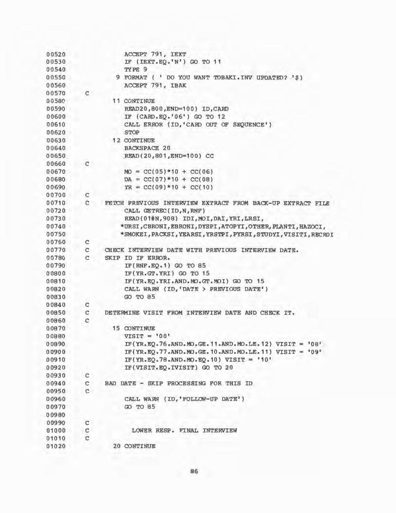
00520 00530 00540 00550 00560 00570 0058(1 00590 00600 00610 00620 00630 00640 00650 00660 00670 00680 00690 00700 00710 00720 00730 00740 00750 00760 00770 00780 00790 00800 00810 00820 00830

C

C

C

c

C

C C

00840 C 00850 00860 00870 00880 00890 00900 00910 00920 00930 00940 00950 00960 00970 00980 00990 01000 01010 01020

C

C

C

C C

C C

C

ACCEPT 791, !EXT IF (IEXT.EQ.'N') GO TO 11 TYPE 9

9 FORMAT ( 1 DO YOU WANT TDBAKI.INV UPDATED?'$) ACCEPT 791, !BAK

11 CONTINUE READ20,800,END=100) ID,CARD IF (CARD.EQ. '06') GO TO 12 CALL ERROR (ID, 'CARD OUT OF SEQUENCE' ) STOP

12 CONTINUE BACKSPACE 20 READ(20,801,END=100) CC

MO= CC(05)*10 + CC(06) DA= CC(07)*10 + CC(08) YR= CC(09)*10 + CC(10)

FETCH PREVIOUS INTERVIEW EXTRACT FROM BACK-UP EXTRACT FILE CALL GETREC(ID,N,RNF) READ(01#N,908) IDI,MOI,DAl,YRI,LRSI,

*URSI,CBRONI,EBRONI,DYSPI,ATOPYI,OTHER,PLANTI,HAZOCI, *SMOKEI,PACKSI,YEARSI,YRSTPI,PYRSI,STUDYI,VISITI,RECRDI

CHECK INTERVIEW DATE WITH PREVIOUS INTERVIEW DATE. SKIP ID IF ERROR.

IF(RNF.EQ.1) GO TO 85 IF(YR.GT.YRI) GO TO 15 IF(YR.EQ.YRI.AND.MO.GT.MOI) GO TO 15 CALL WARN (ID, 'DATE > PREVIOUS DATE') GO TO 85

DETERMINE VISIT FROM INTERVIEW DATE AND CHECK IT.

15 CONTINUE VISIT = '00' IF(YR.EQ.76.AND.MO.GE.11.AND.MO.LE.12) VISIT= '08' IF(YR.EQ.77.AND.K:>.GE.10.AND.MO.LE.11) VISIT= '09' IF(YR.EQ.78.AND.MO.EQ.10) VISIT= '10' IF(VISIT.EQ.IVISIT) GO TO 20

BAD DATE - SKIP PROCESSING FOR THIS ID

CALL WARN (ID, 1 FOLLOW-UP DATE' ) GO TO 85

LOWER RESP. FINAL INTERVIEW

20 CONTINUE

86

01030 01040 01050 01060 01070 01080 01090 01100 01110 01120 01130 01140

C C

01150 C 01160 01170 01180 01190 01200 01210 01220 01230 01240 01250 01260 01270 01280 01290 01300 01310 01320 01330 01340 01350 01360 01370 01380 01390

C

C C

C

C 01400 C 01410 01420 01430 01440 01450 01460 01470 01480 01490 01'500 01510 Q1520 01530

C C C

LRS = 0 IF (CC(13).EQ.1.0R.CC(14).EQ.1.0R.CC(16).EQ.1.0R.CC(17).EQ.1

*.OR.CC(26).EQ.1.0R.CC(29).EQ.1.0R.CC(31).EQ.1) *LRS = 1

IF (CC(13).EQ.2.AND.CC(14).EQ.2.AND.CC(16).EQ.2.AND. * CC(17).EQ.2,AND.CC(29).EQ,2,AND.CC(31).EQ.2.AND. * (CC(26).EQ.2.0R.CC(26).EQ.9)) *LRS = 2

IF ( LRS • NE. 0 ) GO TO 2 5 CALL EXCEPT (ID, 1 LCMER RESP. SYMPTOM 1 )

URS - FINAL INTERVIEW

25 CONTINUE URS= 0 IF (CC(34).EQ.1,0R.CC(36).EQ.1) URS= 1 IF ((CC(34).EQ.2.0R.CC(34).EQ.9).AND.CC(36).EQ,2) URS= 2 IF (URS. NE. 0) GO TO 30 CALL EXCEPT (ID, 'UPPER RESP. SYMPTOM')

BRON. - FINAL INTERVIEW

30 CONTINUE COUGH=O; PHLEG=O; CBRON=O; EBRON=O IF ((CC(13).EQ.1.0R.CC(14).EQ.1).AND.CC(15).EQ.1) COUGH= 1 IF ((CC(16).EQ.1oOR.CC(17).EQ,1).AND.CC(18).EQ.1) PHLEG = 1 IF ((CC(13).EQ.1.0R.CC(13).EQ,2).AND.

* (CC(14).EQ.1.0R.CC(14).EQ.2).AND.

* (CC(15).EQ.2.0R.CC(15),EQ,9)) COUGH= 2 IF ( (CC( 16) .EQ.1.0R.CC( 16) .EQ.2) .AND.

* (CC(17).EQ.1.0R.CC(17).EQ.2).AND.

* (CC(18).EQ.2.0R.CC(18).EQ,9)) PHLEG = 2 IF (COU~.EQ.1.AND.PHLEG.EQ.1) EBRON= 1 IF (COUGH.EQ.2.0R. PHLEG.EQ,2) EBRON= 2 IF (EBRON.EQ.O) CALL EXCEPT (ID, 'CURRENT BRONCHITIS')

DYSPNEA GRADE ( 1=NO, 2-5=YES)

DYSP = 0 CC25=CC(25); CC26=CC(26); CC27=CC(27); CC28=CC(28) IF (CC25.EQ.2.AND.CC26.EQ.9.AND.CC27.EQ.9.AND.CC28.EQ.9) DYSP=1 IF (CC25.EQ.1.AND.CC26.EQ.2,AND.CC27.EQ.9.AND.CC28.EQ.9) 0SYP=2 IF (CC25.EQ.1.AND.CC26.EQ.1.AND.CC27.EQ.2.AND.CC28.EQ.9) DYSP=3 IF (CC25.EQ,1.AND.CC26.EQ.1,AND.CC27.EQ,1.AND.CC28.EQ.2) DYSP=4 IF (CC25.EQ.1.AND.CC26.EQ.1.AND.CC27.EQ.1.AND.CC28.EQ.1) DYSP=S IF (DYSP.EQ.O) CALL EXCEPT (ID,'DYSPNEA GRADE')

40 CONTINUE

SMOKI'OO UPDATE

SMOKE=O; PACKS=99.99; YEARS=99.99; YRSTP=99.99; PYRS=-1 .OO

87

01540 01550 01560 01570 01580 01590 01600 01610 01620 01630 01640 01650 01660 01670 01680 01690 01700 01710 01720 01730 01740 01750 01760 01770 01780 01790 01800 01810 01820 01830 01840 01850 01860 01870 01880 01890 01900 01910 01920 01930 01940 01950 01960 01970 01980 01980 01990 02000 02010 02020

C

C C C C

C

C

C

C

C

C

C

C

C

C C C C

IF(CC(54).EQ.1.AND.CC(55).EQ.1) SMOKE= 1 IF(CC(54).EQ.1.AND.CC(55).EQ.2.AND.

* (CC(59).EQ.1.0R. CC(64).EQ.1)) SMOKE 2 2 IF(CC(54).EQ.2.AND.CC(55).EQ.9.AND.CC(59).EQ.9.AND.CC(64).EQ.9)

*SMOKE= 3 IF (SMOKE.NE.0.AND.SMOKEI.NE.O) GO TO 50 IF (SMOKEI.EQ.O) SMOKE= 0 CALL EXCEPT (ID,'(F)SMOKING STATUS') GO TO 81

DIF EQUALS DIFFERENCE BETWEEN FOLLOW-UP INTERVIEW AND THE PREVIOUS INTERVIEW IN YEARS. S1 IS THE # CIGARETTES SMOKED/DAY •

50 CONTINUE DIE- = (YR-YRI)*360 + (MO-M0I)*30 + (DA-DAI) DIF = DIF /360. SI= CC(56)*10 + CC(57)

IF((SMOKE.EQ.3.0R.SMOKE.EQ.2).AND. * (SMOKEI.EQ.2.0R.SMOKEI.EQ.3)) GO TO 79

IF(SMOKE.EQ.1.AND.SMOKEI.EQ.1) GO TO 60

IF((SMOKE.EQ.2.0R.SMOKE.EQ.3).AND. *(SMOKEI.EQ.1)) GO TO 65

IF(SMOKE.EQ.1.AND.(SMOKEI.EQ.2.0R.SMOKEI.EQ.3)) *GO TO 70

CIGARETTE SMOKER BOTH VISITS

60 CONTINUE CDRRENT SMOKER LAST VISIT IF (YRSTPI.EQ.O.O) YEARS = DIF PAST SMOKER LAST VISIT IF (YRSTPI.GT.O.O.AND.YRSTPI.LT.99.99) YEARS= DIF/2. IF (S1.GT.O.AND.S1.NE.77.AND.S1.NE.88.AND.S1.NE.99) GO TO 62 CALL EXCEPT(ID, "(F)PACKS/DAY SMOKED') GOTO 63

62 PACKS= S1/20. 63 YRSTP = 0 .O

GO TO 80

STOPPED SMOKING BETWEEN VISITS

65 CONTINUE PACKS = PACKS I 7 SMOKE = SMOKE I IF (PACKS.EQ.99.99J CALL EXCEPT (ID,'(F)PACKS/DAY SMOKED')

88

02030 02040 02050 02060 02070 02080 02090 02100 02110 02120 02130 02140 02150 02160 02170 02180 02190 02200 02210 02220 02230 02240 02250 02260 02270 02280 02290 02300 02310 02320 02330 02340 02350 02360 02370 02380 02390 02400 02410 02420 02430 02440 02450 02460 02470 02480 02490 02500 02510 02520 02530

C

C

C

C

C

C

C C

C

C C

C

C

C C

IF (YRSTPI.EQ.O.O) GO TO 66 IF (YRSTPI.GT.O.O.AND.YRSTPI.LT.99.99) GO TO 67 ERROR ON LAST VISIT YEARS STOPPED SMOKING CALL EXCEPT (ID,'(F)YRS STOPPED SMOKE') 00 TO 80 OJRRENT SMOKER LAST VISIT

66 CONTINUE YEARS = DIF /2. YRSTP = DIF/2. 00 TO 80 PAST SMOKER LAST VISIT

67 CONTINUE YEARS=0.07 PACKS-0.0 YRSTP = YRSTPI + DIF IF (YEARS.EQ.99.99) CALL EXCEPT (ID,'(F)YEARS SMOKED') GO TO 80

STARTED SMOKING BE'IWEEN VISITS

70 CONTINUE IF(S1.GT.O.AND.S1.NE.77.AND.S1.NE.88.AND.S1.NE.99) GO TO 72 CALL EXCEPT (ID,'(F)PACKS/DAY SMOKED') 00 TO 73

72 PACKS= S1/20. 73 YRSTP = 0 .O

YEARS = DIF/2. 00 TO 80

NEVER SMOKED IN EITHER VISIT

79 CONTINUE PACKS = 0 .O YEARS = 0 .O YRSTP = 99.99 IF (SMOKEI.EQ.2) SMOKE= 2 00 TO 80

PACK-YEARS UPDATE

80 CONTINUE IF (PACKS.EQ.99.99.0R.YEARS.EQ.99.99) GO TO 81 PYRS = PACKS*YEARS

WRITE ON TO EXTRACrION FILE

81 CONTINUE IF (IEXT.NE. 'Y') GO TO 85 STUDY = 1 08' PLANT= 0.0 HAZOCC = 0 Rl!J:ORD = '0 8'

89

02540 02550 02560 02570 02580 02590 02600 02610 02620 02630 02640 02650 02660 02670 02680 02690 02700 02710 02720 02730 02740 02750 02760 02770 02780 02790 02800 02810 02820 02830 02840 02850 02860 02870 02880 02890 02900

C C

C C C

C

C

C C

C C

C C

C C

C 02910 C 02920 02930 02940 02950 02960 029,70 02980 03000 03010 03020 03030 03040 03050

C

C C C

C C

C 03060 C

WRITE (21,908) ID,MO,DA,YR,LRS,URS,CBRON,EBRON,DYSP,ATOPY, *OTHER,PLANT,HAZOCC,SMOKE,PACKS,YEARS,YRSTP,PYRS, *STUDY,VISIT,RECORD

BACK-UP EXTRAC'r FILE UPDATE IF (IBAK.NE. 1 Y1 ) GO TO 85 WRITE (01#N,908) ID,MO,DA,YR,LRS,URS,CBRON,EBRON,DYSP,ATOPY,

*OTHER,PLANT,HAZOCC,SMOKE,PACKS,YEARS,YRSTP,PYRS, *STUDY,VISIT,RECORD

85 CONTINUE SKIP RECORD 20 GO TO 11

HERE ON END-OF-FILE

100 CONTINUE CALL EXIT END

*************************** SUBROUTINE ERROR(ID,MESSAG) ***************************

TYPES 00T ERROR MESSAGE ON TTY WITH ALPHANUMERIC ID. MESSAGE MUST BE LONGER THAN 10 CHARAC'rERS TO WORK, OTHERWISE YOU MAY GET GARBAGE.

DIMENSION MESSAG(2) DOUBLE PRECISION MESSAG TYPE 1, ID,MESSAG

1 FORMAT (/ 1 *** ERROR ID ',A4,': ',2A10) RETURN END

**************************** SUBROUTINE EXCEPT(ID,MESSAG) ****************************

TYPES 00T EXCEPTION MESSAGE ON TTY WITH ALPHANUMERIC ID. MESSAGE MUST BE LONGER THAN 10 CHARAC'rERS TO WORK, OTHERWISE YOU MAY GET GARBAGE.

DIMENSION MESSAG(~) DOUBLE PRECISION MESSAG TYPE 1, ID,MESSAG RETURN END

*****************•******** SUBROUTINE WARN(ID,MESSAG) **************************

90

03070 03080 03090 03200 03110 03120 03130 03140 03150 03160 03170 03180 03190 03200

C

C

C

C

C

C

C

03210 C 03220 03230 03240 03250 03260 03270 03280 03290 03300 03310 03320 03330 03340 03350 03360 03370 03380 03390 03400 03410 03420 03430 03440 03450 03460 03470 03480 03490 03500 03510 03520 Q3530 03540 03550 03560 03570 03580

C

C

C

C C

C C

C

C C C

C C

C C

C

C

C C

C

TYPES OUT WARNING MESSAGE ON TTY WITH ALPHANUMERIC ID. MESSAGE MUST BE LONGER THAN 10 CHARACTERS TO WORK, OTHERWISE YOU MAY GET GARBAGE.

DIMENSION MESSAG(2) DOUBLE PRECISION MESSAG TYPE 1, ID MESSAG

1 FORMAT(/' * WARNING ID ',A4,': ',2A10) RETURN END

************************* SUBROUTINE TABGEN (!FILE)

*************************

GENERATES LOOK-UP TABLE FOR RANDOM ACCESS BASED ON S~UENTIAL SCAN FOR ID# - PAIRS ID# WITH RECORD #. THIS SUBROUTINE SHOULD BE CALLED ONLY ONCE.

CALLING S~UENCE: CALL TABGEN(IFILE)

WHERE !FILE = INTEX;ER, DOUBLE PRECISION VARIABLE CONTAINING NAME OF FILE TO BE SCANNED.

IN THE LABELLED COMK>N /RAND/: MAXID = INTEX;ER VARIABLE CONTAINING MAX # OF CASES (ID#' S).

MUST BE LESS THAN 1000 (LINEAR DIM OF TABLE ARRAY). TABLE( 1000,2) =- 2-D INTFnER ARRAY LINKING ID# WITH ITS RECORD #

IN FILE.

IMPLICIT INTEX;ER (A-Z) DOUBLE PRECISION !FILE COMK>N /RAND/ MAXID, TABLE(1000,2)

800 FORMAT (A4) 900 FORMAT (/' ERROR IN SUBROUTINE TABGEN: ') 901 FORMAT(' ID ',A4,' HAS APPEARED TWICE IN DATA FILE ',A10.

*',RECORD# ',16 1 AND ',16,'.') 90 2 FORMAT ( ' # OF CASES > MAX # SET UP FOR TABLE. ' )

INITIALIZATION

OPEN (UNIT=1,ACCESS= 1 S~IN' ,FILE=IFILE) IF(MAXID.LE.O) MAXID = 1000 DO 10 1=1,MAXID

TABLE(I,1)= 1 0000' TABLE(I,2)=0

10 CONTINUE I = 0 N = 0 ID2 = •ooo•

91

03590 03600 03610 03620 03630 03640 03650 03660 03670 03680 03690 03700 03710 03720 03730 03740 03750 03760 03770 03780 03790 03800 03810 03820 03830 03840 03850 03860 03870 03880 03890 03900 03910 03920 03930 03940 03950 03960 03970 03980 03990 04000

C

C

C

C C C

C C

C

C C C

C C

C C C

04010 C 04020 04030 040.ilO 04050 04060 04070 04080 04090

C

LOOP UNTIL YOU FIND A DIFFERENT ID. N IS THE RECORD#.

100 CONTINUE N = N+1 READ (1,800,END=999) ID1 IF(ID1.EQ.!D2) GO TO 100

HERE TO MAKE TABLE ENTRIES. CHECK IF ID HAS BEEN ENTERED BEFORE.

200 CONTINUE DO 300 K=1,I

IF (TABLE(K,1).NE.ID1) GO TO 300 TYPE 900 TYPE 901, ID1,IFILE,TABLE(K,2),I STOP

300 CONTINUE I = I+1 TABLE(I,1) = ID1 TABLE(I,2) = N ID2 = ID1

CHECK IF INDEX > MAX. OONTINUE SCAN IF NOT.

IF (I.LE.MAXID) GO TO 100 TYPF. 900 TYPE 902 STOP

HERE ON EOF FOR CLOSE-OTJT.

999 OONTINUE CLOSE (UNIT=1) RETURN END

*************************** SUBROUTINE GETREC(ID,N,RNF) ***************************

SEARCHES TABLE GENERATED BY SUBROUTINE TABGEN FOR ID# AND RETRIEVES RECORD # FOR RANDOM ACCESS.

IMPLICIT INTJ!X;ER (A-Z) OOMK>N /RAND/ MAXID,TABLE(1000,2)

:RNF = 0 DO 10 I=1,MAXID

IF(TABLE(I,1).NE.ID) GO TO 10 N = TABLE(I,2) RETURN

92

04100 04110 04120 04130 04140 04150 04160 C 04170 C 04180 04190 C 04200 C 04210 C 04220 C 04230 04240 04250 04260 04270

10 CONTINUE TYPE 900, ID

900 FORMAT(/' RECORD NOT FOUND FOR ID ',A4) RNF = 1 RETURN END

********************************* SUBROUTINE AERR)R(ID,MESG1,MESG2) *********************************

TYPES OUT ERR'.>R MESSAGE ON TTY WITH ALPHANUMERIC ID

DOUBLE PRECISION MESG1 ,MESG2 TYPE 900, ID,MESG1 ,MESG2

900 FORMAT (/ 1 ERROR ID ',A4,': ',2A10) RETURN END

References

1. Cotes, J.E.: Lung Function Assessment and Application in Medicine. Blackwell Scientific Publications, 1975, Oxford.

2. Knudson, R.J., Slatin, R.C., Lebowitz, M.D., and Burrows, B.: The Maximal Expiratory Flow-Volume Curve - Normal Standards, Variability, and Effects of Age. Amer.Rev.Resp.Dis. 113, 587-600, 1976. ~

3. Fletcher, C., Peto, R., Tiner, c., and Speizer, F.: The Natural History of Chronic Bronchitis and Emphysema. Oxford University Press, 1976, Oxford.

4. Berry, G.: Longitudinal Observations, Their Usefulness and Limita­tions with Special Reference to the Forced Expiratory Volume. Bull. Physio-path. resp., 10, 643-655, 1974

5. Berry, G,, McKerrow, C.B., Molyneux, M.K.B., Rossiter, C.E., Tombleson, J,B.C.: A study of acute and chronic changes in ventilatory capacity of workers in Lancashire cotton mills. Brit.J.Industr.Med.: 30, 25-36, 1973.

6. Butcher, B.T., Jones, R.N., O'Neil, C.E., Glindmeyer, H.W., Diem, J.E., Dharmarajan, V., Weill, H. and Salvaggio, J.E.: Longitudinal study of workers employed in the manufacture of toluene diisocyanate. Amer.Rev.Resp.Dis., 116, 411-421, 1977.

7. Weill, H., Salvaggio, J., Neilson, A., Butcher, B.T., and Ziskind, M.: Respiratory effects in toluene diisocyanate manufacture: A multi­disciplinary approach. Env. Health Perspectives, 11, 101-108, 1975.

8. Butcher, B.T., Salvaggio, J.E., Weill, H. and Ziskind, M.M.: Toluene diisocyanate (TD!) pulmonary disease: Immunologic and inhalation challenge studies. J. Allergy Clin.Immunol., 58, 89-100, 1976.

9. Butcher, B. T.: Immunologic aspects of toluene diisocyanate (TDI) sensitivity in exposed workers at a TD! plant. Proceedings of the Fifth Annual Workshop of the Asthma and Allergic Disease Centers. Pub. NIAID, U.S.D.H.E.W. pp. 171-175, 1975.

10. Butcher, B.T.: cyanate (TDI).

Inhalation challenge testing with toluene diiso­J, Allergy Clin.Immunol., (In Press) 1979.

94

11. Butcher, B.T., Karr, R.M., O'Neil, C.E., Wilson, M.R., Dharmarajan, V., Salvaggio, J.E. and Weill, H.: Inhalation challenge and pharmacologic studies of toluene diisocyanate (TDI) sensitive workers. J. Allergy Clin. Immunol. 64, 146-152, 1979.

12. Butcher, B.T., Salvaggio, j.E., O'Neil, C.E., Weill, H. and Garg, O: Toluene diisocyanate (TDI) pulmonary disease: Immunopharmacologic and mecholyl challenge studies. J, Allergy Clin. Immunol. ~. 223-230, 1977.

13. Butcher, B.T. and Karr, R.M.: TDI induced asthma, in "Diagnosis and management of industrial, drug and radiation hazards - selected topics." Volume 1. Grune and Stratton. (In Press), 1979.

14. Davies, R.J., Butcher, B.T., O'Neil, C.E. and Salvaggio, J.E.; The in vitro effect of toluene diisocyanate on lymphocyte cyclic adenosine monophosphate production by isoproterenol, prostaglandin and histamine -- a possible mode of action. J, Allergy Clin. Immunol. 60, 233-239, 1977.

15. Beaven, M.A., Jacobsen, S. and Horakova, Z: Modification of the enzymatic isotopic assay of histamine and its application to measurement of histamine in tissues, serum and urine. Clin. Chim. Acta,]]_, 91, 1972.

16. Karr, R.M., Davies, R.J., Butcher, B.T., Lehrer, S.B., Wilson, M., Dharmarajan, V., and Salvaggio, J.E.: Allergy Grand Rounds -Occupational Asthma. J. Allergy Clin. Immunol., 61, 54-65, 1978.

17. Mitchell, J.C. and Jordan, W.P.: Allergic contact dermatitis from radish, Raphanus saturis. Brit. J. Dermatol. 91, 183-189, 1974.

18. Butcher, B.T., O'Neil, C/E., Karr, R.M., Weill, H., and Salvaggio, J.E.: Longitudinal study of isocyanate sensitive worker with concurrent development of food allergy shows loss of pharmacologic and metha­choline reactivity. (In preparation).

19. Karol, M.H., Ioset, M.M., and Alarie, i'.''.C.; Tolyl-.specific IgE antibodies in workers with hypersensitivity to toluene diisocyanate. Am. Ind. Hyg. Assoc. J., 39, 454, 1978.

20. Butcher, B.T., O'Neil, C.E. and Salvaggio, J.E.: Radioallergosorbent testing (RAST) of TDI reactive individuals using p-tolyl-isocyanate (TMI) antigen. J. Allergy Clin. Immunol., (Submitted), 1979.

95

21. Weill, H., Salvaggio, J., Neilson, A., Butcher, B., and Ziskind, M.; Respiratory effects in toluene diisocyanate manufacture: A multi­disciplinary Approach. Environ. Hlth. Perspect. 11, · 101--108, 1975.

22. Butcher, B.T., Jones, R.N., O'Neil, C.E., Glindmeyer, H.W., Diem, J.E., Dharmarajan, V., Weill, H., and Salvaggio, J.E.: Longitudinal study of workers employed in the manufacture of toluene diisocyanate •

. Am. Rev. Resp. Dis., 116, 411-421, 1977.

23. Dharmarajan, V.: Analysis of TDI and MDI in air. Am.Ind.Hyg.Assoc.J., 38, 725, 1977.

24. Dharmarajan, V., Weill, H., and Self, C.W.: Environmental character­ization of toluene diisocyanate in a manufacturing plant. Am. Ind. Hyg. Assoc. J., 39, 414-418, 1978.

25. Neilson, A. and Booth, K.S.: A technique for dynamic calibration of a continuous toluene diisocyanate monitor. Am. Ind. Hyg. Ass·oc. J. 36, 169-171, 1975.

26. Dharmarajan, V. and Rando, R.J. A new method for the generation of standard atmospheres of organo isocyanates. Am. Ind. Hyg. Assoc. J, (In Press), 1979.

27. Dharmarajan, V.: Occupational exposures to methylene bisphenyliso­cyanate (MDI): Gaseous or aerosol? J, Environ. Pathol. and Toxicol. l, 1-8, 1979.

28. Marcali, K.: Microdetermination of toluene diisocyanate in atmospheres. Anal. Chem.~. 552-558, 1957.

29. Reilly, D.A.: A test-paper method for the determination of toluene diisocyanate vapor in air. Analyst,~ 178-185, 1968.

30. Allshuller, A.P. and Cohen, I.R.: Application of diffusion cells to the production of known concentrations of gaseous hydrocarbons. Anal. Chem., 32, 802-810, 1960.

31. Model 7000 TDI Monitors are distributed in U.S.A. by MDA Scientific, Inc., 808 Busse Highway, Park Ridge, Ill., 60068.

32. Dixon, W.J.: BMDP, Biomedical Computer Programs, University of California Press, Berkeley, 1975.

33. IMSL Reference Manual, Edition 6, International Mathematical and Statistical Libraries, Houston, 1977.

96

34. Graybill, Franklin A.: An Introduction to Linear Statistical Models Vol 1, McGraw-Hill Book Company, Inc., 1961, New York.

35. Kauffmann, F., Drouet, D., Lellouch, J., and Brille, D.: Twelve years spirometric changes among Paris area workers. Int. Journ. of Epid. ~, 201-202, 1979.

36. Ferris BG, Chen H, Puleo Sand Murphy R L H. Chronic Non specific Respiratory Disease in Berlin, New Hampshire, 1967 to 1973. A further Follow-up study. American Review of Respiratory Disease 114, 475, 1976.

37. Higgins ITT, Gilson JC, Ferris BG, Waters ME, Campbell Hand Kiggins· M w·. IV. Chronic respiratory disease in an industrial town: a nine-year follow-up study. Preliminary Report. American Journal of Public Health 58: 1667, 1968.

38. Petty TL, Pierson DJ, Dick NP, Hudson L D and Walker SH. Follow-up evaluation of a prevalence study for chronic bronchitis and Chronic Airways Obstruction. American Review of Respiratory Disease 114: 881, 1976.

39. Lebowitz MD. Longitudinal changes in lung function and respiratory symptoms. Paper presented IEA Meeting, Puerto Rico, SepteUlher 1977.

40. Pham Q T, Benis A M, Muir J M, Sadoul and Haluska J. Follow-up study of construction workers with obstructive lung disease. Scandinavian Journal of Respiratory Diseases 58:215, 1977.

97

\D 00

Visit Date

Number Added

Permanently Lost

Eligible from Previous Visit

Total Eligible

Refused (% of Elig. from Prev.)

Temporarily Lost (% of Elig. from Prev.)

Complete Spirometry (% of Total Eligible)

Complete Spirometry (% of Eligible -Refused - Temp. Lost)

4-73 11-73

168 27

- 6

- 162

168 189

0 3 (1.9)

2 11 (1.2) (6.8)

144 145 (85.7) (76.7)

144 145

(86. 7) (82.8)

Tpble 1

PARTICIPATION BY VISIT

SPIROMETRY

9-74 3-75 10-75

25 34 23

9 3 11

180 202 225

205 236 248

7 12 21 (3. 9) (5.9) (9.3)

13 21 17 (7. 2) (10.4) (7. 6)

168 197 200 (81. 9) (83.5) (80.6)

168 197 200

(90.8) (97. 0) (95.2)

3-76. 11-76 12-77 10-78 TOTAL

- - - - 277

13 7 13 9 71

235 228 215 206

235 228 215 206

25 37 35 36 (10. 6) (16. 2) (16.3) (17.5)

24 25 34 29 (10.2) (11. O) (15.8) (14 .1)

175 161 142 135 (74.5) (70.6) (66.0) ( 65. 5)

175 161 142 135

(94.1) (97. 0) (97.3) (95.7)

Table 2

DESCRIPTIVE STATISTICS AT INITIAL VISIT FOR THE 274 MALE PARTICIPANTS

1. Race:

2. Cigarette Smoking:

3. Atopy (positive to 2 or more skin tests)

4. Upper respiratory symptoms

5. Lower respiratory symptoms

6. Bronchitis

7. Dyspnea

8. Age (years)

9. Height (inches)

10. Pack-years

11. IgE IU/ml

12. FEV% P(l)

13. FVC% P

14. FEF25_75% P

15. RV% P

16. TLC% P

17. DLco% P

18. K% P

85%

51.1%

22.6%

25.9%

20.1%

38.7%

29.6%

3.6%

84.3%

11.7%

2.9%

274

274

273

271

244

244

244

217

217

212

212

white

current

Ex

Never

Atopic

Positive

Positive

Positive

GRADE I

GRADE II

GRADE III

Mean

35.9

69.9

14.37

181.8

100.2

102.7

91.0

99.4

101.0

99.0

99.7

274

273

274

273

272

273

271

Standard Deviation

11.3

2.56

16.3

287.7

13.3

12.3

26.5

25.7

11.6

16.7

17.3

(l)% predicteds are taken from the pulmonary function measurements at the time of the initial interview or the next visit at which the pulmonary function measurement was taken if it was not done at the visit of the initial interview.

99

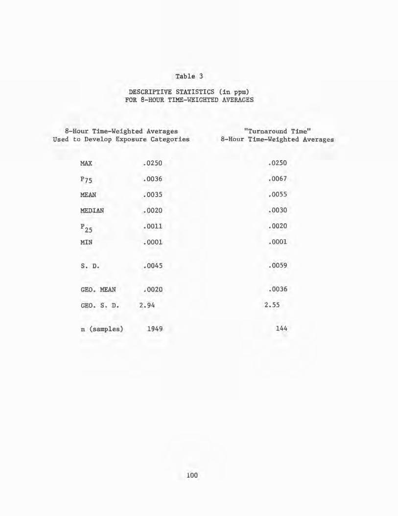
Table 3

DESCRIPTIVE STATISTICS (in ppm) FOR 8-HOUR TIME-WEIGHTED AVEP-~GES

8-Hour Time-Weighted Averages Used to Develop Exposure Categories

"Turnaround Time" 8-Hour Time-Weighted Averages

MAX

P75

MEAN

MEDIAN

p25

MIN

S. D.

GEO. MEAN

GEO. S. D.

n (samples)

.0250

.0036

.0035

.0020

.0011

.0001

.0045

.0020

2.94

1949

100

.0250

.0067

.0055

.0030

.0020

.0001

.0059

.0036

2.55

144

Table 4

JOB TITLES BY TIME-WEIGHTED AVERAGE EXPOSURE CATEGORY

Number Exposure Job of Category Code Job Location Samples

HIGH 13001 C Operator TDI 222 15050 E Operator Drumming 199 15051 E Operator Tank Farm 5 31030 Millwright Phosgene 12 33030 Welder Phosgene 1

MODERATE 1001 Foreman TDI 239 12001 B Operator TDI 208 14030 D Operator Phosgene 224 30001 Unsp. Maint. TDI 7 30021 Unsp. Maint. Machine Shop 4 31001 Millwright TDI 51 32001 Boilermaker TDI 17 33001 Welder TDI 31 34001 Pipefitter TDI 30 36001 Instruments TDI 7 36019 Instruments Shop 5 41002 Unspec. Sampl. TDI Lab 7 42002 A Sampler TDI Lab 14 43002 B Sampler TDI Lab 7

LOW 1014 Foreman Soda Ash 4 1017 Foreman TlOl 4

11001 A Operator TDI 69 11010 A Operator TDA 60 12020 B Operator Hyco 88 13010 C Operator TDA 89 13040 C Operator POL-DNT 14 14040 D Operator POL-DNT 124 15010 E Operator TDA 35 15030 E Operator Phosgene 1 19052 Operator Bug Pond 99 31012 Millwright Sodium Nitrate 2 33009 Welder Ammonia 6 33027 Welder Pilot Plant 3 35001 Electrician TDI 15 35018 Electrician Shop 6 36009 Instruments Ammonia 6 37028 Carpenter Shop 4 40002 Chemist TDI Lab 15 53029 Clerical CAR Warehouse 2 57012 Truck Driver Sodium Nitrate 4 58012 Warehouseman Sodium Nitrate 5 71021 Machinist Shop 4

101

Table 5

8-HOUR TIME-WEIGHTED AVERAGE DESCRIPTIVE STATISTICS (in ppm) BY EXPOSURE CATEGORY

CATEGORY HIGH MODERATE LOW

MAX. .0250 .0250 .0248

p75 .0088 .0035 .0020

MEAN .0068 .0032 .0016

MEDIAN .0050 .0020 .0013

p25 .0025 .00130 .0007

MIN. .0001 .0001 .0001

s. D. .0062 .0039 .0018

GEO. MEAN .0045 .0020 .0011

GEO. S. D. 2.69 2.68 2.37

n 439 851 659

102

Category I:

Category II:

Category III:

Category IV:

Table 6

JOB TITLES BY PEAK EXPOSURE CATEGORY

15050 30001 31030 33030

12001 13001 31001 33001 34001

01001 14030 15051 32001 37001 42002

01014 01017 11001 11010 12020 13010 13040 14040 15010 15030 19052 30021

31010 31012 33009 33010 33020 33027 35001 35018 36001 36009 36019 36020 36030 37028 38001 39001 40002 41002 43002 53029 57012

58012 71021

E Operator in Drumming Unspecified Maintenance in TDI Millwright in Phosgene Welder in Phosgene

B Operator in TDI C Operator in TDI Millwright in TDI Welder in TDI Pipe Fitter in TDI

Foreman in TDI D Operator in Phosgene E Operator in TK Farm Boilermaker in TDI Carpenter in TDI A Sampler in TDI Lab

Foreman in Soda Ash Foreman in T-101 A Operator in TDI A Operator in TDA B Operator in HYCO C Operator in TDA C Operator in POL-DNT D Operator in POL-DNT E Operator in TDA E Operator in Phosgene Operator in Bug Pond Unspecified Maint. in

Machine Shop Millwright in TDA Millwright in Sodium Nitrate Welder in Ammonia Welder in TDA Welder in HYCO Welder in Pilot Plant Electrician in TDI Electrician in Electric Shop Instruments in TDI Instruments in Ammonia Instruments in Instr. Shop Instruments in HYCO Instruments in Phosgene Carpenter in Carpenter Shop Insulator in TDI Maint. Supervisor in TDI Chemist/Analyst in TDI Lab Unspecified Sampler in TDI Lab B Sampler in TDI Lab Clerical in CAR Warehouse Truck Driver or Laborer in

Sodium Nitrate Warehouseman in Sodium Nitrate Machinist in Machine Shop

103

Table 7

Percentage of Time Spent Above Selected Concentration Levels by Peak Exposure Category

Percentage of time above: Number of

Category .005 ppm .01 ppm .02 ppm .04 ppm .06 ppm .08 ppm Samples

I 36.1 20.1 10.6 5.5 3.9 3.4 219

II 24.0 12.1 5.0 2.4 1.6 1.4 618

III 10.7 4.0 1.4 0.5 0.3 0.2 518

IV 3.2 0.7 0.3 0.1 0.1 0.0 738

All Categories Combined 14.6 6.9 3.0 1.4 1.0 0.8 2093

104

Table 8

ANNUAL CHANGE REGRESSION COEFFICIENTS(!) USING CUMULATIVE EXPOSURE, ATOPIC STATUS AND PACK-YEARS AS EXPLANATORY VARIABLES

FEV1 L/yr

FVC L/yr

FEV% (yr)-l

FEF25_75

L/sec-yr

FEF50

L/sec-yr

-1 K (min-nunHg-yr)

ml DLco min-nunHg-yr

E.V L/yr

TLC L/yr

(RV/TLC) x 100 (yr)-l

n

223

223

223

223

223

164

164

179

179

179

Cumulative Intercept Exposure

-.0103 (-1.09)

-.0039 (-. 40)

-.2041 (-1. 52)

-.0736 (-3.23)

-.1115 (-3. 50)

-.169 (-4.99)

-1.127 (-4. 97)

.0391 (3.09)

.0275 (1. 81)

.4400 (3.04)

-.0770 (-.81)

.0455 (: 47)

-1. 372 (-1. 01)

-.00275 (-1.19)

-.000386 (-.12)

1. 276 (3. 31)

7.926 (3. 07)

-.126 (-.99)

.00371 (. 02)

-1.112 (-. 77)

Atopy

.0011 ( .15)

-.0070 (-. 97)

.1246 (1. 21)

.0249 (1.44)

.0374 (1. 54)

-.0155 (-.58)

-.433 (-2.43)

-.00222 (-. 24)

-.0106 (-.93)

-.0181 (-.17)

Pack­Years

-.00057 (-2.55)

-.00071 (-3.13)

-.00332 (-1.03)

-.00024 (-.43)

-.00036 (-.48)

-.00072 (-. 85)

-.0015 (-. 27)

.00104 (3.58)

.00048 (1. 38)

.0114 (3.44)

% Variability Explained

7.36

20.3

3.0

4.1

6.5

28.8

47.5

30.9

5.5

46.4

(l)The numbers in parentheses are the regression coefficients divided by their standard errors. They should be compared to normal distribution percentiles for tests of significance.

105

Table 9

ANNUAL CHANGE REGRESSION COEFFICIENTS(l) USING DICHOTOMIZED CUMULATIVE EXPOSURE, ATOPIC STATUS, AND PACK-YEARS AS EXPLANATORY VARIABLES

Cumulative(2) Exposure Pack- % Variability

n Intercept Category II Atopy Years Explain eel

FEVl L/yr 223 -.0120 -.0118 .0009 -.00058 9.4 (-2.14) (-1. 82) ( .13) (-2.60)

FVC L/yr 223 -.0006 .0012 -.0069 -.00071 19.2 (-.10) ( .19) (-.95) (-3.17)

FEV% (yr) -1 223 -.2358 -.2024 .1216 -.0034 6.30 (-2.94) (-2.20) (1.19) (-1.08)

FEF25-75 L/sec-yr 223 -.0801 -.0406 .0243 -.00025 11.1 (-5. 96) (-2.63) (1.42) (-.46)

FEF50 L/sec-yr 223 -.1031 -.0285 .0373 -.00041 6.6 (-5.44) (-1. 31) (1. 55) (-.54)

K (min-mmHg-yr) -1 164 -.0934 .0518 -.00642 -.00101 16.3 (-4.39) (1. 97) (-.24) (-1.19)

' ml DLco min-mmHg-yr 164 -.6578 .3246 -.3755 -.0033 33.6

(-4.64) (1. 86) (-2.09) ('-. 58)

RV L/yr 179 .0286 -.0061 -.00289 .00107 27.1 (3.83) (-. 07) (-.31) (3.67)

TLC L/yr 179 .0278 .0000 -.0105 .00048 5.6 (3.11) (.00) (-.93) (1.38)

(RV/TLC) x 100 (yr)-l 179 .3331 .0313 -.0246 .0117 41. 7 (3.93) (.32) (-. 23) (3.52)

(1) (1) See Footnote of Table 8.

<2) Cumulative Exposure Category II has value if qJIDulative exposure is > • 0682 ppm-months and O otherwise. Thus, its coefficient estimates the difference between the two cate­gories after controlling for the other variables.

106

Table 10

ANNUAL CHANGE REGRESSION COEFFICIENTS(l) USING THREE CU}!ULATIVE EXPOSURE CATEGORIES(2), ATOPIC STATUS, AND PACK-YEARS AS EXPLANATORY VARIABLES

Cwnulative( 2) Cumulative( 2) Exposure Exposure Pack- % Variabilit

n Interce2t Category II A Categorv II B Ato2:z Years Exelained FEV

1 L/yr 223 -.0123 -.0187 .0132 .0020 -.00057 13 . .::

(-2.21) (-2.25) (1. 31) (. 28) (-2.59)

FVC L/yr 223 -.0008 -.0049 .0115 -.0060 -.00072 21.1 (-.15) (-. 56) (1.10) (-.82) (-3.17)

FEV% (yr) -1 223 -.2374 -.2339 .0597 .1262 -.0034 7.0 (-2.97) (-1.95) (.41) (1.23) (-1. 07)

FEF25-75 L/sec-yr 223 -.0806 -.0494 .0166 .0256 -.00024 13.0 (-6.00) (-2.46) (.68) (1. 49) (-. 44)

FEF50 L/sec-yr 223 -.1032 -.0304 .0035 .0377 -.00041 6.7

(-5.44) (-1.07) (.10) (1.56) (-. 54)

-1 164 -.0921 -.0308 .1407 -.00870 -.00107 35.1 K unin-mmHg-yr )_ (-4.46) (-.·86) (3.26) (-. 33) (-1.29)

ml DLco m~n-mmHg-yr 164 -.6468 -.208 .9013 -.3892 -.00370 66.1

(-4.68) (-. 86) (3.12) (-2.22) (-. 67)

RV L/yr 179 .0288 .00467 -.00951 -.00334 .00107 27.1 (3.85) (.40) (-. 69) (-. 35) (3. 65)

TLC L/yr 179 .0276 -.00860 .0154 -.00978 .00049 5.5 (3.10) (-. 62) (.94) (-. 87) (1.40)

(RV/TLC) x 100 (yr)-l 179 .3359 .1122 -.1455 -.0312 .0117 43.8 (3. 97) (.86) (-. 93) (-.29) (3.51)

(l)See Footnote (l) of Table 8.

(2)cumulative Exposure Category II A has value 1 if cumulative exposure is >.0682 ppm-months and O otherwise. Cumulative Exposure Category II B has value 1 if cumulative exposure is >.1 ppm-months and O otherwise. The coefficient of Cumulative Exposure Category II A (resp. Cumulative Exposure Category II B) estimates the difference between the two lowest (resp. highest) categories after controlling for the other variables.

107

Table 11

ANNUAL CHANGE REGRESSION COEFFICIENTS(l) USING TIME ABOVE .02 ppm, ATOPIC STATUS, AND PACK-YEARS AS EXPLANATORY VARIABLES

Time Above Pack- % Variability n Intercept .02 ppm Atopy Years Explained

FEV1 L/yr 223 -.0141 -.0043 .0010 -.00057 9.51

(-2.51) (-1.05) ( .14) (-2.56)

FVC L/yr 223 -.0020 .0032 -.0070 -.00071 19.7 (-. 35) (. 75) (-. 96) (-3.12)

FEV% L/yr 223 -.2470 -.452 .1231 -.0035 6.2 (-3.09) (-1. 93) (1. 24) (-1.08)

FEF25-75 L/sec-yr 223 -.0853 -.0184 .0246 -.00024 7.6 (-6. 31) (-1.83) (1. 42) (-. 44)

FEF50 L/sec-yr 223 -.1107 -.0066 .0375 -.00038 4.7 (5.83) (-. 47) (1. 55) (-. 50)

K (min-mmHg-yr)-1 164 -.0968 .0380 -.00832 -.00095 16.6 (-4. 47) (2.14) (-. 31) (-1.10)

ml 164 -.6482 .1761 -.382 -.00305 DLco - min-mmHg-yr - 27.3

(-4.45) (1. 48) (-2.11) (-.53)

RV L/yr 179 .0361 -.0129 -.0017 .00102 38.1 (4. 93) (-2.38) (-.19) (3.55)

TLC L/yr 179 .0322 -.00733 -.00996 .00045 9.9 (4.69) (-1.11) (-. 88) (1.29)

(RV/TLC) x 100 (yr) -1 179 .4238 -.1361 -.0114 .0112 55.4 (5. 08) (-2. 20) (-.11) (3.40)

(l)See Footnote (l) of Table 8.

108

Table 12

ANNUAL CHANGE REGRESSION COEFFICIENTS(l) USING DICHOTOMIZED TIME ABOVE .02 ppm, ATOPIC STATUS, AND PACK-YEARS AS EXPLANATORY VARIABLES

Peak Exposure(2) Pack- % Variability n Intercept Category II Atopy Years Explained

FEV1 L/yr 223 -.0127 -.0108 .00058 -.00058 10.9

(-2.29) (-1.64) (.08) (-2.61)

FVC L/yr 223 .0005 -'.0015 -.0069 -.00072 18.6 ( .09) (-.22) (-. 95) (-3.18)

FEV% yr -1 223 -.2594 -.1541 .1158 -.0034 6.0 (-3. 26) (-1. 63) (1.13) (-1.07)

FEF25-75 L/sec-yr 223 -.0847 -.0317 .0232 -.00024 10.0 (-6. 34) (-1.99) (1. 35) (-.45)

FEF50 L/sec-yr 223 -.0999 -.0396 .0.361 -.00045 8.7 (-5.34) (-1. 77) (1. 50) (-. 60)

K (min-mrnHg-yr) -1 164 -.0977 .0646 -.0058 -.00101 24.3 (-4.64) (2.50) (-.22) (-1.19)

ml 164 -.6560 -.3706 DLco min-mmHg-yr • 3170 -.00338 31. 4

(-4, 64) (1. 82) (-2.06) (-.60)

RV L/yr 179 .0341 -.0172 -.00285 .00104 32.4 (4.69) (-1. 92) (-. 30) (3.60)

TLC L/yr 179 .0331 -.0158 -.0105 .00045 11. 3 (3.81) (-1.48) (-. 94) (1. 31)

(RV/TLC) x 100 (yr) -1 179 , 3911 -.1427 -.0240 .0115 44.2 (4. 70) (-1.40) (-. 22) (3.46)

(l)See Footnote (1) of Table 8.

(2)Peak Exposure Category II has value 1 if time above .02 ppm is> .19 months and O other-wise. Thus, its coefficient estimates the difference between the two categories after controlling for the other variables.

109

Table 13

ANNUAL CHANGE REG~SSION COEFFICIENTS(l) USING THREE TIME ABOVE .02 ppm CATEGORIES, ATOPIC STATUS, AND PACK-YEARS AS EXPLANATORY VARIABLES

Peak Exposure Peak Exposure Pack- i; Variability n Intercept Category II A Category II B Atopy Years Explained

FEV1

L/yr 223 -.0127 -.0139 .0070 .00042 -.00057 10. 7 (-2. 30) (-1. 71) (.65) (.06) (-2. 57)

FVC L/yr 223 .0003 -.0088 .0167 -.0073 -.00071 18.5 (.06) (-1.05) (1.49) (-1. 00) (-3.11)

FEV% (yr) -1-

223 -.2581 =.0972 -.0129 .1185 -.0035 6.3 (-3.25) (-.84) (-. 84) (1.16) (-1.11)

FEF25-75 L/sec-yr 223 -.0847 -.0303 -.0031 .0233 -.00024 9.9 (-6. 34) (-1.55) (-.12) (1. 35) (-. 46)

1--' 1--' 0 FEF50 L/sec-yr 223 -.1005 -.0682 .0660 .0345 -.00037 11. 7

(-5. 40) (-2.50) (1. 80) (1. 44) (-.49)

-1 164 -.0975 .0687 -.00979 -.0054 -.00102 24.3 K (min-mmHg-yr) (-4. 63) (2.16) (2. 24) (-. 20) (-1. 21)

ml DLco 164 -.6541 .3615 -.1051 -.3670 -.00357 36.0

min-mm."'lg-yr (-4.62) (1. 69) (-. 36) (-2.05) (-.63)

RV L/yr 179 .0345 -.00661 -.0242 -.00166 .00100 39.5 (9. 81) c....:. 61) (-1.63) (-.18) (3.48)

TLC L/yr 179 .0332 -.0128 -'.00679 -.0102 .00044 12.5 (3.83) (-. 97) (-. 38) (-. 91) (l.2z}

(RV/TLC) x 100 (yr)-l 179 . 3952 -.00866 -.3102 -.00783 .0109 57.8 (4.84) (-. 07) (-1.82) (-.07) (3.33)

(1) (1) See Footnote of Table 8

(Z)Peak Exposure Category II A has value 1 if time above .02 ppm> .19 months and O otherwise. Peak Exposure Category II B has value of time above .02 ppm> 1 month and O otherwise. Thus, the coefficient of peak Exposure Category II A (resp., Peak Exposure Category II B) estimates the difference between the two lowest (resp. highest) categories after controlli~g for the other variables.

Table 14

ESTIMATED POPULATION MEAN ANNUAL CHAi.~GES AND OTHER STATISTICS

Estimated Percent of(l) Standard Residual Degrees of Total Variability

Estimated Standard Deviation Error Freedom in Due to True Mean Annual Error of Mean of True Annual Standard Residual Sum Annual

n Change Annual Change Cha~ge Deviation of Sguares Change

FEV1 L/yr 223 -.0244 .00316 .0255 .1326 928 49.5

FVC L/yr 223 -.0121 .00330 .0272 .1372 928 51.0

FEV% (yr) -1 223 -.3928 .0451 .3985 1. 7752 928 57.1

FEF25-75 L/sec-yr 223 -.0928 .00762 ,0598 .3242 928 47.5

.... FEF50 L/sec-yr 223 -.1100 .0106 .0790 .4653 928 43.3 .... ....

K (min-mmHg-yr) -1 164 -.0947 .0123 .0757 .3651 301 53.2

ml DL CO min-nnn..llg-yr

164 -. 7160 .0834 .4629 2.559 301 46.4

RV L/yr 179 .0435 .00434 .0306 .1616 448 48.6

TLC L/yr 179 :0322 .00498 .0328 .1910 448 43.9

(RV/TLC) x 100 (yr)-l 179 .5121 .0495 .2925 1.980 448 36.6

(l)Percent of total variability due to true annual change for a participant with usable data at all nine visits. For a participant present at fewer than nine visits, the percent of total variability due to true annual c' ange will be smaller.

Table 15

Summary Statistics on 274 Participants by Number of Visits with Complete Spirometry

Number of Number of visits ~3 visits <3

n 226 48

% White 85.4 83.3

% Lower Respiratory Symptoms 29.8 29.8

% Upper Respiratory Symptoms* 42.0 23.4

% Bronchitis 3.5 4.3

% Interview Atopic 33.8 25.5

% Atopic* 23.0 6.3

% Dyspnea 14.3 17.0

% Current Cigarette Smokers 50.9 53.2

Number of visits ~3 Number of visits

Standard (1) Standard Mean Deviation n Mean Deviation

Age (years) 35.6 11.0 226 35.5 12.6

Height (inches) 70.0 2.5 226 69.8 2.9

Pack-years 13.7 14.9 226 17.4 21.9

FEV1

% P(2) 100.4 13.4 207 99.2 13.3

FVC % p 102.9 12.4 207 101.4 12.0

FEF % p 91.5 26.9 207 88.2 24.5

RV% P 99.3 25.2 186 100.4 28.8

TLC% P 101.3 11.6 186 99.5 11.6

K % p 99.7 17.7 181 99.7 14.2

Cumulative Exposure* (ppm-months) .0725 .0354 225 .0231 .0169

Time above .02 ppm (months)* .55 • 72 225 .29 .33

*p <.05

(l)n represents number of participants with usable data.

<3

n

48

48

47

37

37

37

31

31

31

30

30

(2) % predicteds are taken from the pulmonary function measurement at the time of the initial interview or the next visit at which the pullllonary function measure­ment was taken if it was not done at the visit of the initial interview.

112

FEV%

n

ml/yr

ml/yr

(yr)-1

FEF25_75 ml/sec-yr

FEF50 ml/sec-yr

Table 16

ESTIMATED MEAN ANNUAL CHANGES IN SPIROMETRIC TESTS BY

TWO CUMULATIVE EXPOSURE CATEGORIES FOR NON-ATOPICS WITH

14 PACK-YEARS OF SMOKING

GROUP I

(ppm-months~ .0682)

149

-20

-11

-0.28

-84

-109

(p = .034>1

(p = 1.0)

(p, = .014)

(p = • 004)

(p = • 095)

GROUP II

(ppm-months> .0682)

74

-32

-9

-.48

-125

-137

1 p-values are significance levels for one-tailed tests of significance for differences between the two groups after controlling for other variables.

113

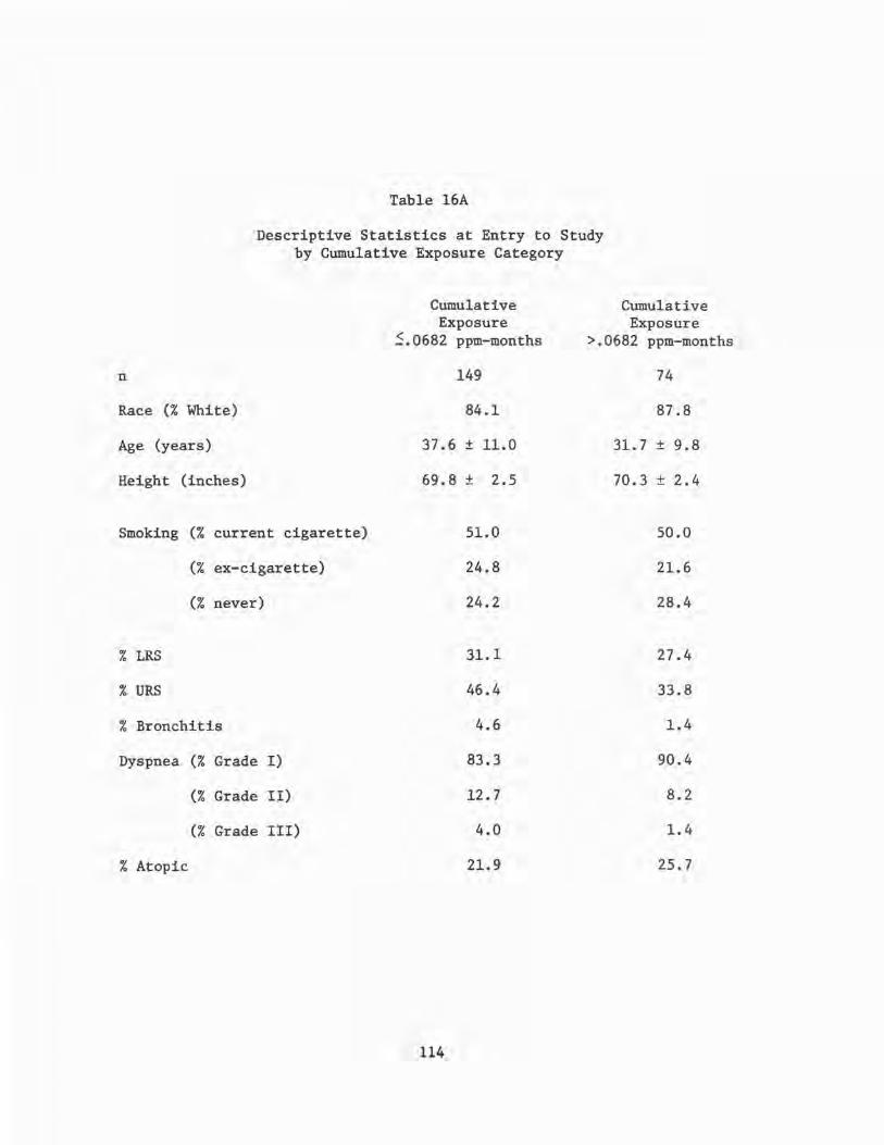
Table 16A

Descriptive Statistics at Entry to Study by Cumulative Exposure Category

n

Race(% White)

Age (years)

Height (inches)

Smoking (% current cigarette)

(% ex-cigarette)

(% never)

% LRS

% URS

% Bronchitis

Dyspnea (% Grade I)

(% Grade II)

(% Grade III)

% Atopic

Cumulative Exposure

~.0682 ppm-months

149

84.1

37.6 ± 11.0

69.8 ± 2.5

114

51.0

24.8

24.2

31. l

46.4

4.6

83.3

12.7

4.0

21.9

Cumulative Exposure

>.0682 ppm-months

74

87.8

31. 7 ± 9. 8

70.3 ± 2.4

50.0

21.6

28.4

27.4

33.8

1.4

90.4

8.2

1.4

25.7

C I G A R '.E T T E

s M 0 K I N G

never

ex

Table 16B

FEV1 Slope (ml/year)* by Smoking Exposure Category Controlling for Age and FEV

1 Level

Exposure

:'.::. 0682 ppm-months

1

n = 35

-12

n = 31

-26

>.0682 ppm-months

-37

n = 21

-15

n = 16

-37

FEV1 level

FEV /h3 <55 1

Exposure

~.0682 ppm-months

>.0682 ppm-months

-18 -57

n = 1 n = 0

-32 -35

n = 6 n = 0

-46 -57 current

n = 64 n = 35 n = 12 n = 2

*Cells means were estimated using the multiple regression procedure described in the text. This procedure used age as one of the covariates. The cells means presented above are adjusted to the average age (35.6 years) of the study group.

Tests of Significance

(1) age effect -5.8 ml/decade one-tailed p-value = .03

(2) low FEV1 effect -20 ml/year one-tailed p-value = .04

(3) exposure effect in never smokers -38 ml/year one-tailed p-value = .001

(4) Smoking effect in ~.0682 exposure category

exsmoker - never smoker effect -13 ml/year one-tailed p-value = .12

current smoker - ex-smoker effect -14 ml/year one-tailed p-value = .06

current smoker-never smoker effect -27 ml/year one-tailed p-value = .004

115

Table 17

ESTIMATED MEAN ANNUAL CHANGES IN FEV1, FEV%, AND FEF25_75 BY CUMULATIVE EXPOSURE FOR NON-ATOPICS WITH 14 PACK-YEARS OF SMOKING

GROUP I GROUP II A GROUP II B (ppm-months S.0682) ( .0682 < ppm-months S.1) (ppm-months

n 149 37 37

FEV1 ml/yr -20 (p = .025) 1 -39 (p = .19) -26

FEV% (yr) -1 -.29 (p = .OS) -.52 (p = .68) -.46

FEF25

_75

ml/sec-yr -84 (p = .014) -133 (p = .50) -117

(l)p-values are significance levels for differences between adjacent categories after controlling for other variables.

116

> .1)

Table 18

ESTIMATED MEAN ANNUAL CHANGES IN SPIROMETRIC TESTS BY TWO TIME ABOVE .02 ppm CATEGORIES

FOR NON-ATOPICS WITH 14 PACK-YEARS OF SMOKING

GROUP I GROUP II (months S.19) (months >.19)

n 140 83

FEV1 -21 (p = .051) 1 -32

FVC -10 (p = .413) -11

FEV% -.31 (p = .052) -.46

FEF25-75 -88 (p = • 023) -120

FEF50 -106 (p = .038) -146

(l)p-values are significance levels for one-tailed tests of significance for differences between the two groups after co~trolling for the other variables.

117

n

FEV1 ml/yr

FEV% (yr) -1

Table 19

ESTIMATED MEAN ANNUAL CHANGES IN FEV1 , FEV%, FEF25_75 , AND FEF50 BY TIME ABOVE .02 ppm

CATEGORY FOR NON-ATOPICS WITH 14 PACK-YEARS OF SMOKING

GROUP I GROUP II A (months ~.19) (.19 < months ~1)

140 47

-21 (p = .087) -35 (p = .52)

-.31 (p = .40) -.40 (p = .40)

FEF25-75 ml/sec-yr -88 (p = .12) -118 (p = .90)

FEF50 ml/sec-yr -106 (p = .012) -174 (p = .072)

GROUP II B (months >1)

36

-28

-.42

-121

-108

(l)p-values are significance levels for differences between adjacent categories after controlling for other variables.

ll8

Table 20

SUMMARY STATISTICS ON 274 PARTICIPANTS BY NUMBER OF VISITS WITH COMPLETE DIFFUSING CAPACITY

DETERMINATIONS

Number of Visits ~3

Number of Visits <3

n

% White

% Lower Respiratory Symptoms

% Upper Respiratory Symptoms*

% Bronchitis

% Interview Atopy

% Atopic

% Dyspnea

% Current Cigarette Smokers

165

88.5

29.3

46.7

4.2

34.5

24.8

14.6

48.5

109

80.7

30.6

26.9

2.8

29.0

12.7

14.9

55.6

Number of Visits ~3 Standard (1)

Number of Visits <3 Standard

Mean

Age (years) 36.0

Height (inches) 70.1

Pack-years 14.0

FEV1% P(2) 100.7

FVC % P 103.2

FEF % P 91.1

RV% P 100.0

TLC% P 102.0

K % P 99.9

Cumulative Exposure* (ppm-months) .068

Time above .02 ppm (months) .49

Deviation

11.0

2.5

15.0

12.7

12.1

26.1

24.5

11. 7

17.4

.031

.67

n

165

165

165

151

151

151

139

139

135

164

164

Mean Deviation

35.9

69.7

14.9

99.5

101.8

90.9

99.0

100.0

99.4

.039

.42

11.8

2.6

18.2

14.4

12.7

27.4

27.9

11.5

17.1

.023

.49

* p < .05

(1) n represents the number of participants with usable data.

n

109

109

108

93

93

93

78

78

77

77

77

<2)% predicteds are taken from the pulmonary function measurement at the time of the initial interview or the next visit at which the pulmonary measurement was taken if it was not done at the visit of the initial-interview.

119

Table 21

SUMMARY STATISTICS ON 274 PARTICIPANTS BY NUMBER OF VISITS WITH COMPLETE LUNG VOLUME DETERMINATIONS

Number of Visits Number of Visits :::3 <3

n 182 92

% White 87.4 81.5

% Lower Respiratory Symptoms 28.7 31.9

% Upper Respiratory Symptoms* 44.0 28.6

% Bronchitis 3.8 3.3

% Interview Atopy 34.1 28.9

% Atopic 24.2 12.0

% Dyspnea· 13.3 17.7

% Current Cigarette Smokers 48.4 57.1

Number of Visits ~3 Number of Visits Standard (1) Standard

Mean Deviation n Mean Deviation

Age {years) 35.7 11.0 182 36.5 11.9

Height (inches) 70.1 2.5 182 69.5 2.6

Pack-years 13.5 14.8 182 16.2 19.0 FEV

1%(2) 101.3 12.9 165 98.0 14.0

FVC % p 103.6 12.3 165 100.8 12.3

FEF % p 92.0 25.9 165 88.9 28.0

RV% P 98.8 24.6 151 100.9 28.3

TLC % p 101. 7 11.6 151 99.5 11.6

K % p 99.5 17.4 146 100.2 17.1

Cumulative Exposure* (ppm-months) .08 .03 181 .03 .02

Time Above • 02 ppm (months) .57 .75 181 .38 .45

*p ~ .05

(l)n represents the number of participants with usable data.

<3

n

92

92

91

79

79

79

66

66

66

60

60

(2)% predicteds are taken from the pulmonary function measurement at the time of the initial interview or the next visit at which the pulmonary function measurement was taken if it was not done at the visit of the initial inter­view.

120

Table 22

SUMMARY STATISTICS ON 274 PARTICIPANTS BY COMPLETENESS OF INITIAL AND FINAL INTERVIEW

Complete Incomplete

n 203 71

% White 87.1 80.3

% Interview Atopy 37.0 30.4

% Atopic 22.2 14.1

% Current Cigarette Smokers 52.2 48.6

Complete Incomplete Standard (1) Standard

Mean Deviation n Mean Deviation

Age (years) 35.4 10.8 203 37.5 12.6

Height (inches) 69.9 2.6 203 69.9 2.4

Pack-years 13.6 14.8 203 16.5 20.1

FEV1% p(2) 100.5 13.4 182 99.5 13.4

FVC % p 103.1 12.0 182 101.6 13.2

FEF % p 91.4 27.2 182 89.8 24.6

RV% P 98.6 25.8 165 102.2 25.7

TLC % p 101.5 11.5 165 99.7 11.9

K % p 100.1 16.9 160 98.7 18.6

Cumulative Exposure* (ppm-months) .082 .033 202 .013 .015

Time Above .02 ppm* (months) . 62 .80 202 .019 .19

* p < .05

(l)n represents the number of participants with usable data.

n

71

71

70

62

62

62

52

52

52

23

23

(2)% predicteds are taken from the pulmonary function measurements at the time of the initial interview or the next visit at which the pulmonary function measurement was taken if it was not done at the visit of the initial inter­view.

121

Last Initial Usable Zero INTRVW INTRVW PK-YRS

YES YES 7 u

YES NO 0 R

NO YES 3 s

NO NO 6

YES YES 1 L

YES ·NO 0 R

NO YES 2 s

NO NO 13

YES E YES 0 B

YES NO 0 R

NO YES 1 0

NO NO 15 N

YES D YES 0 y

YES NO 1

s NO YES 1

NO p

NO 14

Table 23

LONGITUDINAL C~GE IN SYMPTOMS BY CUMULATIVE EXPOSURE CATEGORY

Cumulative Exposure~ .0682

Non-Atopic Atopic

0-15 > 15 Zero 0-15 > 15 Zero

Cumulative Exposure> .0682

Non-Atopic Atopic

0-15 > 15 Zero 0-15 PK-YRS PK-YRS PK-YRS PK-YRS PK-YRS TOTAL PK-YRS PK-YRS PK-YRS PK-YRS PK-YRS

15 20 2 4 3 51 2 5 10 3 4

3 0 2 1 0 6 1 0 1 0 0

9 7 2 6 1 28 8 8 3 2 2

9 11 2 0 3 31 9 14 6 1 4

8 9 0 5 2 25 1 2 5 1 4

7 4 3 1 1 16 0 7 0 0 0

10 7 1 1 1 22 3 3 6 0 0

11 18 4 4 3 53 16 15 9 5 5

0 0 0 1 0 1 0 0 0 0 0

5 1 0 0 0 6 0 1 0 0 0

0 5 0 1 0 7 1 2 1 1 1

31 32 8 9 7 102 19 24 19 5. 9

5 5 0 0 0 10 1 3 2 0 0

1 2 1 2 0 7 0 0 3 0 0

3 5 2 1 1 13 1 4 5 1 2

27 26 5 8 6 86 18 20 10 5 7

122

>15 PK-YRS TOTAL

1 25

1 3

0 23

1 35

1 14

0 7

1 13

1 51

0 0

0 1

1 7

2 78

0 6

0 3

2 15

1 61

Last Initial Usable INTRVW INTRVW

YES YES u

YES NO R

NO YES s

NO NO

YES YES

L YES NO

R NO YES

s NO NO

YES E YES B

YES NO R

NO YES 0

NO NO N

YES D YES y

YES s NO

NO p

YES N

NO E NO A

Table 24

LONGITUDINAL CHANGE IN SYMPTOMS BY TIME ABOVE .02 ppm CATEGORY

Time above .02 ppm ~ 0.19 Time above .02 > 0.19

Non-Atopic Atopic Non-:-Atopic A;opic

Zero 0-15 >15 Zero 0-15 >15 Zero 0-15 >15 Zero 0-15 PK-YRS PK-YRS PK-YRS PK-YRS PK-YRS PK-YRS TOTAL PK-YRS PK-YRS PK-YRS PK-YRS PK-YRS

6 16 22 3 5 3 55 3 4 8 2 3

0 2 0 2 1 1 6 1 1 1 0 0

4 10 7 2 5 1 29 7 7 3 2 3

9 11 11 2 1 3 37 6 12 6 1 3

2 6 8 1 4 3 24 0 4 6 0 5

0 9 4 3 1 1 18 0 5 0 0 0

2 9 9 1 1 1 23 3 4 4 0 0

15 15 19 4 6 3 62 14 11 8 5 3

0 0 0 0 1 0 1 0 0 0 0 0

0 4 1 0 0 0 5 0 2 0 0 0

1 0 5 1 1 0 8 1 2 1 0 1

18 35 34 8 10 8 113 16 20 17 5 8

0 4 6 0 0 0 10 1 4 1 0 0

1 1 2 1 1 0 6 0 0 3 0 1

2 3 5 2 1 2 15 0 4 5 1 2

16 31 27 6 10 6 96 16 16 9 4 5

123

>15 PK-YRS TOTAL

1 21

0 3

0 22

1 29

0 15

0 5

1 12

1 42

0 0

0 2

1 6

-1 67

0 6

0 4

1 13

1 51

Table 24A

Prevalences for Selected Respiratory Symptom Complexes at the Initial and Final Interviews

by Smoking-Cumulative Exposure Categories

Bronchitis Never Smokers Current or Ex-Smokers

Mean n Initial Final Age n Initial Final

~.0682 ppm-months 24 0% 4.2% 36.2 92 7.6% 7.6%

>.0682 ppm-months 26 0% 7.7% 28.2 60 1. 7% 8.3%

Dyspnea Never Smokers Current or Ex-Smokers

Mean n Initial Final Age n Initial Final

~.0682 ppm-months 24 8.3% 12.5% 36.2 92 16.3% 21. 7%

>.0682 ppm-months 26 3.8% 11.5% 28.2 59 13.6 30.5%

124

Mean Pack- Mean Years Age

20.0 38.9

15.6 33.1

Mean Pack- Mean Years Age

20.0 38.9

15.6 33.1

Table 25

"Clinical Reactors" to TDI

Time in Smoking in Atopic Known Plants

Age Pack-Years Challenge .?2 Skin Major Before Job When I. D. in 1973 <Initial) Results Test Exposure Symptoms Became Symptomatic Comments

0033 47 47 - 0 + <1 week B Op TDI transferred out of TDI, then resigned from plant

0035 26 7 0 0 7 months D Op TDI still works in TDI

0037 27 7 + 0 0 2 months D Op TDI transferred out of TDI then quit for medical reasons

0045 53 11 0 0 "weeks" Foreman TDA transferred out of TDI

0046 26 6 - + + <2 months Chemical Engineer, resigned from plant East Zone

0110 30 8 - + + 4 months Welder TDI/TDA transferred out of TDI

0179 20 0 + 0 3 years C Op TDA still works in TDI

0187 26 0 + + 4 months Pipefitter TDI/TDA transferred out of TDI

0197 61 0 - 0 + 4 months Pipefitter TDI/TDA resigned from plant

0200 32 0 0 0 2~ years Pipefitter TDI/TDA transferred out of TDI

0218 57 0 0 0 3 months Insulator TDI/TDA transferred out of TDI

0256 33 7 0 + 2 years Pipefitter TDI/TDA transferred out of TDI

125

Table 26

TDI Environmental Exposure Evaluation (8/73 to 7/75)

Location

TDI Plant

TDI Drumming Building

Percent Weekly TWA Excursions

Above .005

82.7%

60.3%

126

Percent Weekly TWA Excursions

Above 0.02

24.7%

6.4%

January 7

January 14

January 21

January 28

February 6

February 13

February 20

February 27

March 6

March 13

March 20

March 27

April 5

April 12

April 19

April 26

May 3

May 10

May 17

May 24

Table 27

PERSONNEL MONITORING SCHEDULE

(January 7 - May 28, 1976)

thru January 11 "A" Shift

thru January 18 "B" Shift

thru January 25 "C" Shift

thru February 1 "D" Shift

thru February 10 "D" Shift

thru February 17 "A" Shift

thru February 24 "B" Shift

thru March 2 "C" Shift

thru March 10 "C" Shift

thru March 17 "D" Shift

thru March 24 "A" Shift

' thru March 31 "B" Shift

thru April 9 Maintenance

thru April 16 Maintenance

thru April 23 Maintenance

thru April 30 Maintenance

thru May 7 Drumming Lab

thru May 14 Drumming Lab

thru May 21 Drumming Lab

thru May 28 Drumming Lab

127

4 p.m. - 12 a.m.

4 p.m. - 12 a.m.

4 p.m. - 12 a.m.

4 p.m. - 12 a.m.

8 a.m. - 4 p.m.

8 a.m. - 4 p.m.

8 a.m. - 4 p.m.

8 a.m. - 4 p.m.

12 a.m. - 8 a.m.

12 a.m. - 8 a.m.

12 a.m. - 8 a.m.

12 a.m. - 8 a.m.

8 a.m. - 4 p.m.

8 a.m. - 4 p.m.

8 a.m. - 4 p.m.

8 a.m. - 4 p.m.

8 a.m. - 4 p.m.

8 a.m. - 4 p.m.

8 a.m. - 4 p.m.

8 a.m. - 4 p.m.

Table 28

COMPARISON OF TDI MONITOR VS. PERSONAL MONITOR

Exposure in Minutes Time-

.005 .Cl "" .04 .06 no Total weighted Plant Date • v, .vu

Name oom. avera2e Shift

Area TDI 5-19-75 101.2 32.2 0 0 0 0 .0349 .0044 8 AM 4 PM

Production TDI 5-19-75 324 306 270 207 192 189 .200 .025 8 AM Worker 1 4 PM Production TDI 5-19-75 168 87 54 9 0 0 .054 .0068 8 AM Worker 2 4 PM

Area TDI 5-20-75 16.1 11.5 0 0 0 0 .0139 ,0017 8 AM 4 PM

Production Unknown 5-20-75 195 162 120 39 0 0 .090 .0113 8 AM Worker 1 4 PM Production TDI 5-20-75 330 174 93 39 24 21 .105 .0131 8 AM Worker 2 4 PM

Area TDI 5-22-75 0 0 0 0 0 0 .0104 .0013 8 AM 4 PM

Production Unknown 5-22-75 407 384 183 39 9 0 .154 .0193 8 AM Worker 1 4 PM Production TDI 5-22-75 327 138 48 15 9 9 .080 .010 8 AM Worker 2 4 PM

Area TDI 6-25-75 200.1 140.3 87.4 20.7 0 0 .124 .0155 4 PM 11 PM

Production TDI 6-25-75 4 PM Worker 1 11 PM Production TDI 6-25-75 12 0 0 0 0 0 .019 .0024 4 PM Worker 2 11 PM Production TDI 6-25-75 9 0 0 0 0 0 .018 .0023 4 PM Worker 3 11 PM

Area TDI 6-26-75 190.9 165.6 115 20.7 13.8 13.8 .1213 .0152 4 PM 11 PM

Production TDI 6-26-75 69 15 0 0 0 0 .020 .0025 4 PM Worker 1 11 PM Production Phosgene 6-26-75 36 6 0 0 0 0 .002 .00025 4 PM Worker 2 11 PM Production TDI 6-26-75 207 84 15 0 0 0 .047 .0059 4 PM Worker 3 11 PM Production TDI 6-26-75 51 21 6 0 0 0 .036 .0045 4 PM Worker 4 11 PM

Area Drumming 5-20-75 400.2 299 69 43.7 41.4 41.4 .1490 .0186 8 AM 4 PM

Production Drumming 5-20-75 309 72 45 9 0 0 .066 .0083 8 AM Worker 1 4 PM Production Drumming 5-20-75 174 48 0 0 0 0 .036 .0045 8 AM Worker 2 4 PM Production Drumming 5-20-75 51 30 0 0 0 0 .022 .0028 8 AM Worker 3 4 PM

Area Drumming 5-23-75 11.5 6,9 0 0 0 0 .0297 .0037 8 AM 4 PM

Production Drumming 5-23-75 8 AM

Worker 1 4 PM Production Drumming 5-23-75 360 6 0 0 0 0 .050 .0063 8 AM Worker 2 4 PM Production Drumming 5-23-75 21 0 0 0 0 0 .016 .002 8 AM Worker 3 4 PM

128

Job Title

Phosgene Operator

TD! Operator

DNT Operator

Maintenance

*Shift 1 Shift 2

Table 29

SUMMARY OF PERSONAL MONITORING FOR PHOSGENE IN A TD! MANUFACTURING PLANT

Monitoring Number Number Period of of

Location Month-Year Shifts* Workers Readings

Phosgene 3/76-12/76 1,2,3 10 71 Plant

TD! 3/76- 4/76 1,3 2 6 Plant

TDA 3/76 3 3 14 Plant

TD! and 5/76-12/76 1 6 22 Phosgene Plant

8 a.m. - 4 p.m. 4 p.m. -12 midnight

Shift 3 12 midnight - 8 a.m.

129

Concentration of Phosgene - PPM

Mean 8-hr TWA + SD -

0.004 + 0.004 -

0.004 + 0.003

0.004 + 0.003

0.011 + 0.017 -

HISTOGRAM OF 8-HOUR TIME-WEIGHTED AVERAGES

(LOG-SCALE)

40

30

20

10

Histogram of 1949 a-Hour Time­Weighted Averages Used to Develop Exposure Categories

~ o~~~~~~~...-~-Q5

~ ~

Histogram of 144 II , II

Turn Around Time "' 40 a-Hour Time -

Weighted Averages 30

20

10

oL....,JmJ!IJd~~~~'fA--I 2 3 4 5 6 7 8

Category of Log ( TWA ) Figure 1

130

HISTOGRAM OF 8-HOUR TIME-WEIGHTED AVERAGES BY EXPOSURE CATEGORY

( LOG SCALE) 40

30

20

10

High Exposure ( 439 samples)

o Lm,:,,1/ZJ.~~~~~L

40

......._ 30 ~

Moderate Exposure ( 851 samples }

~ 20

rt 10

oL....r;;Plm~~~~~~L-

40

30

20

10

Low Exposure ( 659 samples)

0 I--.&.~ ~~l'&lV&tlma.--....--

I 2 3 45 67 8

Category of Log ( TWA )

Figure 2

131

FEV1 MEAN BY VISIT FOR THE 33 PARTICIPANTS WITH COMPLETE SPIROMETRY AT ALL NINE VISITS

4.3

4.2

4.1 ~ ~ l( 4.0

3.9

3.8

Mean Annual Change = - .021 I / year

4/73 11/73 9/74 I 10/75 I 11/76 12/77 10/78 3/75 3/76

Visit Date

Figure 3

132

TD I REACTORS

! FEv,I

~ FEV1

! ID 019114"1 '75 3.5~

3.0 • •,

FEF2s-1!i (L/s~cl FEF25-15

5~ '75 4.5 ~ 4.0 • ~~., 4.5K • ~31-[!§"oo] j ' ' ' • 2

'76

3 '76

• ~ • •• ~ • -- • •1 • '75 ~ 'fr 'is I I I I

'74 '74 '75 '76 '77 '78

4.J j10021eJ~~

Year Year

• ""8n to *" al ,_, from TDI

Figure 4

133

TOI REACTORS

~ ~ FEV1

110 0033 J :it._.._ ;~ 3. _.1.'73 .~

....

~ ~

'73 FEF2s-75

2.0 11 I I I I I

-3/ 2 .+ -1~1111

1, .... ,::~ I

'78 3

1,000..Jl· • • • • •. 2 2. •

2 I I I I I 1.5 11 I I I e,

~ !tD of10].4 ~ ~& I

,,._ ~ '75 '76 '77 78

~ Year

'~ '74

5.0~

4.5 1 pre- '74 °75 '76 '77 '78

8JIP.OSU'9 '73

Year

~ Nf9r1 to date of removql from TD I

TDI REACTORS

~ ~ FEV1

FEF25-75 (L/sec)

5.5

FEF 25-75

I I 5.5~ '14 5.o ID 0035 ~ .1. • I ----- • 5.o VJ 4.5 • -------• . . . . . . .

4.5 •, I I I I I 4.0

7.0 ·16 176

~ • I 5.] 6.5 'V j ID O 179 I • - • •

5.0 8 •• • e 6,0 • e •

4.5 I I I I I i 5.5 pre-

174 175 176 '77 178 179 pre-174 175 176 177 178 179

exposure exposure 173 173

Year Year

} refers to date of sensitization to TD I

Figure 5

134

ce:o F

G E

D

C

............ . . . . H . : ' ..........

J

FIGURE 6

SCHEMATIC DIAGRAM OF PROVOCATIVE INHALATION CHALLENGE CHAMBER

135

A= challenge subject

B = observer

C = TDI monitor

D = air pump

E = rotameter

F = TDI container

G = circulation fan

H = exhaust (overhead)

J = air lock

A.

,..,oo .., IL

I so % u

C.

I 50 % u

IIIEIIATE IESPIISE

I 2 3 4 5 6 TIME AFTER CHALLENGE

(HOURS)

DIAL IESPOISE

.. ~ 2345678~

TIME AFTER CHALLENGE (HOURS)

8.

D.

~-100 IL

Ill I 50 C % u

Figure 7

LATE IESNISE

I 2 3 4 5 TIME AFTER CHALLENGE

(HOURS)

DOSE IESNISE

~0.0lppm

J r, 23456 24

TIME AFTER CHALLENGE (HOURS)

Respiratory Response to Provocative Inhalation Challenge with TD!

136

EFFECT OF CROMALYN ON TOI INDUCED ASTHMA

401

30~

FEF (25-75) 20 ,-. ~ Liter~nd

. 10 I

0

sec I I ! IOO

~~---______ I A • / --.........---- ~, \ I f--.o... '

__....____ -~------

Pl.MD> '\ \ l \\

I I

20 IO O 0 IEFORE BPT

BPT

~

10 20 30

Time In Minutes

Figure 8

137

AFTER BPT

~~IO

~ Cont~I [:

~ TOI ~t ..... I 20

0 40 50 .,

°lo

z 0 2 t-<{ ...J :)

::E t-Cl)

~

::E <{ u

~ 0 150

1000

500

IS 0

N N

R

R

10-BM ,o-4M 10-BM I0-4M

TD I

N R - TOI REACTORS

N = NORMALS

Figure 9

Cyclic Adenosine Monophosphate Dose Response Slopes of TDI Reactors and Normal Individuals to Stimulation with Agonists: Isoproterenol,

Prostaglandin E1

, and TDI

138

E ci u

1600 ·

1500.

1400.

1300

1200

1100 ·

1000 ·

900,

800.

700·

600,

500

400,

300,

200

100.

0

TMI/HSA· HSA

METHOD

• • • --------

• •• • •

··1··· •n , .. 'ii~• .... .~t:. REACTOflS CONTROLS

RAST INDEX

• •

•

• --------•••• • •• • •• • • • •••••••• • •• •• • •• •• • •• ••••••• • •••• • • a•

REACTORS CONTROLS

Figure 10

Radioallergosorbent Tests with p-tolyl Monoisocyanate of Sera from TDI Reactors and Controls

139

9

8

:::0 ~ 7 l>

CJ)

-i 6

::, ci a,

5 )(

4

3

2

0

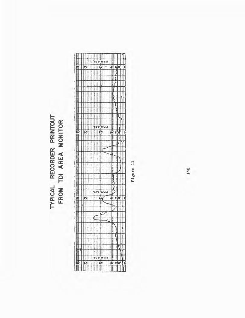
I i i ! 1mm G~

: ! I : ·nn-;w-,r, IO" ~- 11 i i to· lO" ~. ·c

II !I ' I I

ji ii I !, ! I ' ·11 :i i. :111 ii I

; , I I I i ! I : ' ra ' I I

I :

' ~ ::::, a: ~ 0

I--

' I I '

TO\l·:W'cl'cl

80' ~· to· IO'U' 0 ., z a: £L 0

2 a::

I l r

I I! I

I II!: i I I d n

~ <( 0 1'J a: a: 8 <(

~ 0 a:

' : 11 I! Ii I

: . I ' I : . ' 11 1 1: ,: ' I •

! ' ·' 6 I. I I ! : : I ; i, rl li . '

I' I II i!!i I,' I . ~

'! I '' I, , 11 ' !ii 1 I' I '. I' I• I

I-

;rl 2 0 0 it ff >-I-

f I I :fll lli I I

I . 1 I I I. fl I. , I

!,o· TO'J.·;w·c1·c1 ' . J ' I

~· ' t)(' . 10·: soo· 0 ; :"i, ,l.4i iJ, I

I l. .

~ -J.

t I i --~ .. . ' i I :.: ,11 I .......

I ' 1: 1 I I 111 I ;

Ill ii 9

' r 1· I! ,,

I I'

, · . I; I , 111 ! 11 i i : ; ii ' ·1 :1 1 I i I i

i 1 1 i 1 .i! I: ·1111 i

: i ! : ,ii ' .I s ,, i

'' ' TQ'J.·'W'cl'ol I ,, I , ' !,'. ~·:I; I to: li ! 1 ILo·; soo· •

l.llll Ul.i:l lll lllill 111111n11 II

CONCURRENT I MPINGER AND MONITOR TOI LEVELS

(field) .035

• . 030 • ~ .......

t5 • ~ . 025

~ r = .81

• '- . 020

~ ~,,;

.015 },e~

~ o\ .~e

. 010 • ... ,, ....... ~

.005

o~----...._-.---,,-------.---.------.----, 0 .005 .010 .015 .020 .025 .030 .035

TD I , PPM (Monitor) Figure 12

141

-i

1-rj ~ .... rr, I-" ()Q .. ~ C N 11 z (1)

I-' ~ w rr, rr, ~ (/)

8- 13-73

9- I0-73

10- 15-73

11 - 19-73

12-24-73

I - 28-74

TOI CONCENTRATION IN PPM

0 0 N

·-=~~Ii;:=~-;;_:~~

- =-•

0 vi

------------· ---- ....

0 .:.

3- 4-74 ...-----

4- 8-74

5- 13-74

6- 17-74

7- 22-74

8-26-74

9-30-74

11- 4-74

----~-...z~---:.~::::.~

~ ~--=---------.,_ ''I' . .... __

.,..,,.. ... -... 12- 9-74

.:. ___ ..,..

I - 13-75

2- 17-75 II 3-24-75

4-28-75

6- 2-75

7- 7-75

11

9

~ 7 (l)

~ 5

3

7

5

3

5

3

TOI PLANT HISTOGRAM OF WEEKLY TWA

Nov 73 to Sep 74

Mean = 0.0153 ppm

Std, Dev.= 0.0111

Sep 74 to Mar 75 Mean = 0.0223 ppm Std. Dev.= 0.0090

Mar 75 to June 75 Mean = 0.0 I 02 ppm Std. Dev.= 0.0056

l() l() l() l() l() l() ~ l() l() l() l() C) '3- ~ '3- 0) '3- ~

0) ~ 0) C) C) ' ' (\J ~ ~ '3- '3-~ ~ ~ C) C) ~ ~ ~ ~ -

ppm

Figure 14

143

TOI DRUMMING BUILDING HISTOGRAM OF WEEKLY TWA

19 11/5/73 to 8/26/74 17 Mean = 0.0078 ppm

15 Std. Dev. = 0.0096

13

11

9

7

~ 5 Q.)

~

' C)

i..... Mean = 0.0066 ppm Q.)

~ Std. Dev.= 0.0038 § <

7 3/3/75 to 7/21/75

5 Mean = 0.0110 ppm

3 Std, Dev. = 0.0070

le) le) ~ le) ~ le) ~ le) le) le) le)

B ~ ~ ~ ~ O') ~ O') C) C) ....... .......

~ ~ h')

~ "" ~ C) ~ C) ~ C) C) ~ C)

ppm Figure 15

144

TYPICAL RECORDER PRltfTOUT

FROM TOI PERSONAL MONITOR

T.D.I -- DATAGRAM'• "' 0 ----:.c11- -f "C' I: ~ 3· ... .oe n Ei "'

. ..,. • C: ii -< .05 1----:18-

~ "' ·-,- 0

r .d.

II :, er •

~18- 1 I? w ~J ...

i~ - r ,.. -~-::'4- ; ;- 3. .03

"' -o~ II ~ a f~ -... - iil -·- g ~= -- --~ ~~ . --n -... - .. =: 0 -:12~ • :,

0 .. ~ I

-~ --~ ~ -- . Z -0-n _.,,_ ... -"'--.. 02 z . 2 ~·~10--<- '-- --· r--.--

i 0 " > -:a-n ... _

=~~!-. I

?; - -- 0 ' ::! z z 0 -z--

" z .;,-'- =~:;os== i .01 " .01 ic "' I -

-l--:.04-

·1

" 6 \ --,02-

I J" r - I

' "

,._J - - ~ 7

2 3 " C 1 4 I I 1 EI.Al'SED TIME- HRS

• I OWIT NO. IICIII 4tOO ,-qo•u.a.A. MDA 8aENTW'IC INC. PAltll: llllDGI. L eooe8 U.S.A.

Figure 16

145

Q) c~ C\J

C a.>--~

CJ) )(

0:: \ 0 o.Q w \ .c .~o 0 a..

\ (.) z 0: \

I 0

\ I \ 0 \

I

r- CJ) I C\J

\ 0 0 LL 0:: \ z 0~

\ (0

\ "- ....... 0 .-I

CJ) z \ Cl)

\ 1-4 '° WO C\J ::, ..;t

Cl) I() 00 ~

0~ \ u Tl

~ . ::) w \ E tn a.. \ CL

~ \ v CL \

w \ (.) \ z \0 ro w 0:: \

w 0 LL \

0:: \ C\J

w \

r- \

z \ \ \ \ \

0 I() 0 I() 00 C\J Q Q

0 Q Q

( Dl1/pOa8 OOOL /apow)

/0.J. JO wdd 1ua1011,1nb3

TD I DATAGRAM .08-------------­.071-------------------1 .061-------------------1 .05--------------

.04~-----------------t

.03--------------

" .005

~ o....._---~~~--~~------

10 20 30 40 50 60 70 80

Time ( Minutes) Time Scale Expanded

Figure 18

147

EFFECT OF TEMPERATURE ON MODEL 7000 TDI MONITOR

1.6 ................

1.4 ~~ ~t 1.2 ~

C)I 1.0 ~

0.8 r,;::: •:,..... -....::

~ t:s 0.6 "'6 ~

~~

• • e_ No Temperature - - - - - - -.- - -.- - - - - - Effect Line

I • 0.4 -~ 0.2 ' cg 0.0

-10° oo 10° 20° 30°

Temperature °C

Figure 19

148

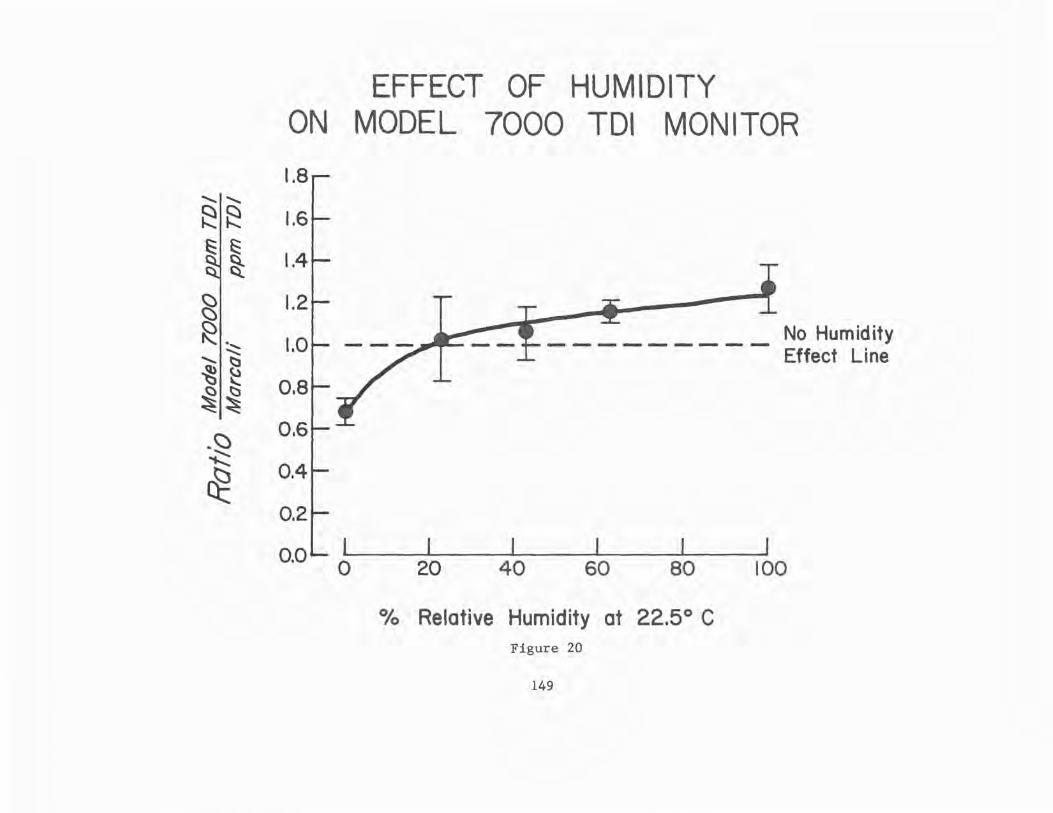
ON

1.8 ..............

~~ 1.6 ~ ~ ~ 1.4

~I 1.2

~ ~ 1.0

....... ~ ~ {.)

(:) ~ 0.8 ~~

-~ 0.6 ~

~ 0.4

0.2

o.ol l 0

EFFECT OF HUMIDITY MODEL 7000 TOI MONITOR

20 40

No Humidity - - - - - - - - - Effect Line

60 80 100

0/o Relative Humidity at 22.5° C Figure 20

149

DISTANCE BETWEEN SELECTED JOBS

40 E-OPERATOR

30 DRUMMING

20

10

0 . 0.,

"') 40 ~ ...... FOREMAN ......: ........ TOI ,,

t:::: 30 s;, •• (l) Cb ~ 20

<I).

~ c3'

~ :::s 10 C')

Cb ."> ,, ~ 0 .

40 BUG POND ~

30 OPERATOR

20

10

0 I 2 3 4 5 6 7 8

Category of Log (TWA) Figure -21

150

,,

DISTANCE BETWEEN SELECTED JOBS

40

30

20

A-OPERATOR TOI

10

oL.i~VAiV&!WM~-------------

40

' ~ 30

0-0PERATOR PHOSGENE

~ 20 ~ "- 10

0

40

30

20

FOREMAN TOI

10

OL......K2'Boll~~'LµU.~rpfU..fLK,ir,c.A--

I 2 345 67 8

-Category of Log ( TWA ) Figure 22

151

,,

REPRINTS INCLUDED IN NIOSH FINAL REPORT - 10/12/79

1. Respiratory Effects in Toluene Diisocyanate Manufacture: A Multidisciplinary Approach - Weill, Salvaggio, Neilson, Butcher, Ziskind

2. Longitudinal Study of Workers Employed in the Manufacture of Toluene­Diisocyanate - Butcher, Jones, O'Neil, Glindmeyer, Diem, Dharmarajan, Weill, Salvaggio

3. Environmental characterization of toluene diisocyanate (TD!) in a manufacturing plant - Dharmarajan, Weill, Self

4. Physical state of airborne p.p' diphenylmethane diisocyanate (MDI) and its measurement - Dharmarajan and Weill

5. Occupational Exposures to Methylene Bisphenylisocyanate (MDI): Gaseous or Aerosol - Dharmarajan

6. Analysis of Toluene Diisocyanate (TDI) and p.p'-Diphenylmethane Diisocyanate (MDI) in Air - Dharmarajan

7. The in vitro effect of toluene diisocyanate on lymphocyte cyclic adenosine monophosphate production by isoproterenol, prostaglandin, and histamine - Davies, Butcher, O'Neil, Salvaggio

8. Occupational asthma caused by low molecular weight chemical agents -Davies, Butcher, Salvaggio

9. Occupational Asthma - Karr, Davies, Butcher, Lehrer, Wilson, Dharmarajan, Salvaggio

10. Toluene diisocyanate (TD!) pulmonary disease: Innnunologic and inhalation challenge studies - Butcher, Salvaggio, Weill, Zisk.ind

11. Toluene diisocyanate Pulmonary Disease: Immunopharmacologic and Mecholyl Challenge Studies - Butcher, Salvaggio, O'Neil, Weill, Garg

12. Inhalation challenge and pharmacologic studies of toluene diisocyanate (TD!) - sensitive workers -- Butcher, Karr, O'Neil, Wilson, Dharmarajan, Salvaggio, Weill

13. Inhalation challenge testing with. toluene diisocyanate CI'DI} -Butcher

14. Radioallergosorbent Testing (RAST} of TDI Reactive Individuals using p-Tolyl Isocyanate (TMI) Antigen - Butcher, O'Neil, Salvaggio

15. A new method for the generation of standard atmospheres of organo isocyanates - Dharmarajan, Rando.

152 o U.&. CIOYEIINMEIIT ""NllNG OFFICE: 1•1 - 757-074/3603

DEPARTMENT OF HEAL TH AND HUMAN SERVICES PUBLIC HEAL TH SERVICE

CENTERS FOR DISEASE CONTROL

NATIONAL INSTITUTE FOR OCCUPATIONAL SAFETY AND HEAL TH ROBERT A. TAFT LABORATORIES

4676 COLUMBIA PARKWAY, CINCINNATI, OHIO 45226

OFFICIAL BUSINESS

PENALTY FOR PRIVATE USE. $300

Special Fourth Class-Book POSTAGE AND FEES PAID U.S. DEPARTMENT OF HHS

HHS 396

DHHS (NIOSH) Publication No. 81-125