Resolution Independent Density Estimation

for Motion Planning in High-Dimensional Spaces

Bryant Gipson, Mark Moll, and Lydia E. Kavraki

Abstract— This paper presents a new motion planner, SearchTree with Resolution Independent Density Estimation (STRIDE),designed for rapid exploration and path planning in high-dimensional systems (greater than 10). A Geometric Near-neighbor Access Tree (GNAT) is maintained to estimate the sam-pling density of the configuration space, allowing an implicit,resolution-independent, Voronoi partitioning to provide sam-pling density estimates, naturally guiding the planner towardsunexplored regions of the configuration space. This planneris capable of rapid exploration in the full dimension of theconfiguration space and, given that a GNAT requires only avalid distance metric, STRIDE is largely parameter-free. Ex-tensive experimental results demonstrate significant dimension-dependent performance improvements over alternative state-of-the-art planners. In particular, high-dimensional systems wherethe free space is mostly defined by narrow passages were foundto yield the greatest performance improvements. Experimentalresults are shown for both a classical 6-dimensional problemand those for which the dimension incrementally varies from3 to 27.

I. INTRODUCTION

In recent years, the field of motion planning [1] has

expanded beyond its roots in low-dimensional geometric

path planning and manipulation to find applications in a wide

variety of seemingly unrelated fields, including biology [2]–

[4], graphics [5] and logic [6], [7]. Much of this expansion

has been driven by the widespread availability of fast motion

planners. One major class of such planners are sampling-

based motion planning algorithms [8], [9].

Originally designed to solve multiple queries in abstract

configuration spaces, Probabilistic RoadMaps (PRM) [10]

represent one of the earliest successful sampling-based motion

planners, establishing a framework for existing work and

paving the way for future developments. Several sampling-

based methods were later developed that were optimized

for single-planning single-query problems. Planners such

as Rapidly Exploring Random Trees (RRT) [11], Expansive

Space Trees (EST) [12] and Single-Query Bi-Directional Lazy

PRM (SBL) [13] represent examples of planners for single

query problems. Many variations of these planners exist—see

for example [8], [9].

Regardless of the method, sampling-based motion planning

algorithms typically share a set of core features: sampling,

where new elements from the configuration space are sampled

and validated, and connection, where connection attempts

are made between new or existing samples yielding a graph-

structure representing the current roadmap or tree. Queries,

B. Gipson, M. Moll and L.E. Kavraki are with Rice University,Department of Computer Science, MS 132, PO Box 1892, Houston TX,77251-1892, USA, kavraki at rice.edu

where useful information is retrieved from the roadmap or tree,

including whether any goals have been satisfied, can occur at

any stage of the process and planners typically incorporate

goal satisfaction checks during execution.

Different planners employ various strategies for sample

generation and connection, but the success of a method (both

in runtime and storage requirements) has been observed to

depend on the topology, distance metric and dimension of

the embedding space and the specific requirements of the

query. Configuration spaces containing disjoint regions of the

free-space, or highly-constrained narrow passage regions are

especially sensitive to the method of sampling, for example.

The planner presented in this paper focuses on the prob-

lem of effective sampling in configuration spaces of high

dimensions (i.e., greater than 10) and in cases where the free

space is defined mostly by narrow passages. Examples of

such configuration spaces include those of highly constrained

kinematic systems such as a robot arm in the interior of

a jet engine, a surgical robot, a point robot navigating a

high-dimensional maze or biological protein systems. In such

cases, uniform random sampling may be inefficient (or fail

altogether) if the ratio of the volume of the free space to that

of the configuration space as a whole is low.

Non-uniform sampling methods have been proposed to

address the problem of generating good samples for certain

classes of configuration spaces. These methods fall into two

categories: importance-based sampling and adaptive sampling.

Importance-based sampling relies on a priori information

about the configuration/workspace and has found success

in methods such as goal-based sampling [14], obstacle-

based sampling [15], Gaussian sampling [16] and medial-axis

sampling [17], among others. In the most general cases,

where the configuration space is complex or the workspace is

implicitly defined, adaptive sampling can be used to sample

new points based only on information related to previously

sampled nodes. Examples of adaptive sampling can be found

in Visibility PRM [18], Cross-entropy motion planning [19],

GPRM [20] and Instance-based Learning [21], among others.

Very fast adaptive sampling, in the form of heuristics

based on sampling density estimation on low-dimensional

projections, has recently shown considerable success. Exam-

ples of such sampling can be found in Kinodynamic Motion

Planning by Interior-Exterior Cell Exploration (KPIECE) [22],

[23], practical implementations of EST [24], methods em-

ploying Principle Component Analysis [25], PDST [26],

SBL [13] and Synergistic Combination of Layers Of Planning

(SyCLoP) [27]. Such methods have been shown to be highly

successful, even in high-dimensional configuration spaces,

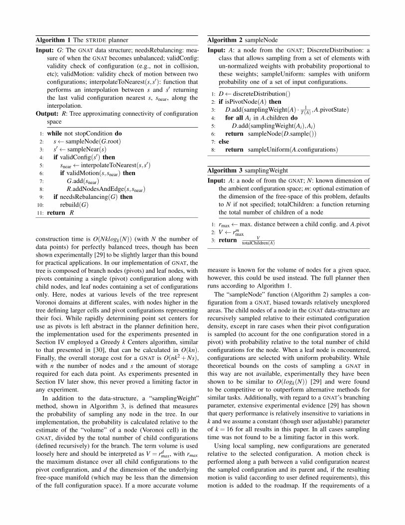
Algorithm 1 The STRIDE planner

Input: G: The GNAT data structure; needsRebalancing: mea-

sure of when the GNAT becomes unbalanced; validConfig:

validity check of configuration (e.g., not in collision,

etc); validMotion: validity check of motion between two

configurations; interpolateToNearest(s,s′): function that

performs an interpolation between s and s′ returning

the last valid configuration nearest s, snear, along the

interpolation.

Output: R: Tree approximating connectivity of configuration

space

1: while not stopCondition do

2: s ← sampleNode(G.root)3: s′ ← sampleNear(s)4: if validConfig(s′) then

5: snear ← interpolateToNearest(s,s′)6: if validMotion(s,snear) then

7: G.add(snear)8: R.addNodesAndEdge(s,snear)9: if needsRebalancing(G) then

10: rebuild(G)11: return R

construction time is O(Nklogk(N)) (with N the number of

data points) for perfectly balanced trees, though has been

shown experimentally [29] to be slightly larger than this bound

for practical applications. In our implementation of GNAT, the

tree is composed of branch nodes (pivots) and leaf nodes, with

pivots containing a single (pivot) configuration along with

child nodes, and leaf nodes containing a set of configurations

only. Here, nodes at various levels of the tree represent

Voronoi domains at different scales, with nodes higher in the

tree defining larger cells and pivot configurations representing

their foci. While rapidly determining point set centers for

use as pivots is left abstract in the planner definition here,

the implementation used for the experiments presented in

Section IV employed a Greedy k Centers algorithm, similar

to that presented in [30], that can be calculated in O(kn).Finally, the overall storage cost for a GNAT is O(nk2 +Ns),with n the number of nodes and s the amount of storage

required for each data point. As experiments presented in

Section IV later show, this never proved a limiting factor in

any experiment.

In addition to the data-structure, a “samplingWeight”

method, shown in Algorithm 3, is defined that measures

the probability of sampling any node in the tree. In our

implementation, the probability is calculated relative to the

estimate of the “volume” of a node (Voronoi cell) in the

GNAT, divided by the total number of child configurations

(defined recursively) for the branch. The term volume is used

loosely here and should be interpreted as V = rdmax, with rmax

the maximum distance over all child configurations to the

pivot configuration, and d the dimension of the underlying

free-space manifold (which may be less than the dimension

of the full configuration space). If a more accurate volume

Algorithm 2 sampleNode

Input: A: a node from the GNAT; DiscreteDistribution: a

class that allows sampling from a set of elements with

un-normalized weights with probability proportional to

these weights; sampleUniform: samples with uniform

probability one of a set of input configurations.

1: D ← discreteDistribution()2: if isPivotNode(A) then

3: D.add(samplingWeight(A) · 1T (A) ,A.pivotState)

4: for all Ai in A.children do

5: D.add(samplingWeight(Ai),Ai)6: return sampleNode(D.sample())7: else

8: return sampleUniform(A.configurations)

Algorithm 3 samplingWeight

Input: A: a node of from the GNAT; N: known dimension of

the ambient configuration space; m: optional estimation of

the dimension of the free-space of this problem, defaults

to N if not specified; totalChildren: a function returning

the total number of children of a node

1: rmax ← max. distance between a child config. and A.pivot

2: V ← rmmax

3: return VtotalChildren(A)

measure is known for the volume of nodes for a given space,

however, this could be used instead. The full planner then

runs according to Algorithm 1.

The “sampleNode” function (Algorithm 2) samples a con-

figuration from a GNAT, biased towards relatively unexplored

areas. The child nodes of a node in the GNAT data-structure are

recursively sampled relative to their estimated configuration

density, except in rare cases when their pivot configuration

is sampled (to account for the one configuration stored in a

pivot) with probability relative to the total number of child

configurations for the node. When a leaf node is encountered,

configurations are selected with uniform probability. While

theoretical bounds on the costs of sampling a GNAT in

this way are not available, experimentally they have been

shown to be similar to O(logk(N)) [29] and were found

to be competitive or to outperform alternative methods for

similar tasks. Additionally, with regard to a GNAT’s branching

parameter, extensive experimental evidence [29] has shown

that query performance is relatively insensitive to variations in

k and we assume a constant (though user adjustable) parameter

of k = 16 for all results in this paper. In all cases sampling

time was not found to be a limiting factor in this work.

Using local sampling, new configurations are generated

relative to the selected configuration. A motion check is

performed along a path between a valid configuration nearest

the sampled configuration and its parent and, if the resulting

motion is valid (according to user defined requirements), this

motion is added to the roadmap. If the requirements of a

user query are satisfied the algorithm stops and returns the

roadmap, otherwise the GNAT is checked for balance (which is

calculated in constant time) and quickly rebuilt from scratch

if required and the algorithm continues. There are many

ways to check for tree balance both abstractly and relative

to the configuration space. The implementation used for the

experiments in Section IV automatically assumed the tree had

become imbalanced when the number of nodes had grown

above 10% of its previous size, leading to a logarithmically

timed rebuilding of the tree and amortized constant cost for

planning overall. This favors balancing that occurs regularly

when the tree is small and prone to imbalance and less

frequently when the tree is large, a method that was found

to be successful in all experiments.

By maintaining a GNAT over the set of configurations

determined in a given round of motion planning, one obtains

both a natural partitioning of the underlying configuration

space and, importantly, local density estimates. Choosing

which configuration to expand from then becomes a process

of sampling GNAT partitions with a heuristic defined relative

to this density (see Algorithm 2 and Algorithm 3). Further,

because density is sampled and estimated recursively at

multiple resolutions, no particular granularity comes to

dominate the sampling process—with samples instead tending

to be drawn naturally from the low-density edges of the

current set of configurations. This results in a sampling

scheme that requires no prior knowledge of spatial topology

or native dimension, but which rapidly and evenly samples

the available free space.

We present STRIDE as a uni-directional planner and

compare its performance in a number of settings against other

single-directional planners. Nothing presented here would

preclude a bi-directional form of this planner, however, though

this is left for future work.

IV. RESULTS

A. Setup

Three experiments were performed in order to compare

dimension dependent differences between a number of

popular planners and STRIDE. For complete generality, we

do not consider problem-optimized planners, such as those

employing inverse kinematics (e.g., [31]). These experiments

were selected in particular to demonstrate cases where STRIDE

is expected to outperform, namely highly constrained high-

dimensional systems. It is this regime that STRIDE was

designed to address and, as the experiments will show, the

type of problem for which STRIDE performs best. The final

simulation shows a more typical 6-dimensional rigid-body

rotational problem for completeness, which nonetheless pos-

sesses enough of the features of the above problems to show

performance differences. It is shown that STRIDE outperforms

(some by orders of magnitude) the alternative planners in

the high-dimensional regime while remaining competitive for

lower dimensions (2–6). Experiments were performed using

the Open Motion Planning Library (OMPL) [24].

The first problem, chosen for theoretical clarity, represents

the model introduced in Section II. Because the space was

0

0.2

0.4

0.6

0.8

1

5 10 15 20 25 30

solv

ed

#dimensions

RRT

PRM

EST

KPIECE

STRIDE

(a) Number of dimensions vs. percentage of runs solved for all availableplanners. STRIDE is consistently at 100% for all dimensions.

0.0001

0.001

0.01

0.1

1

10

100

1000

5 10 15 20 25

tim

e

#dimensions

RRT

PRM

EST

KPIECE

STRIDE

(b) Log plot of number of dimensions vs. time required to solve.

10

100

1000

10000

100000

1e+06

5 10 15 20 25

gra

ph s

tate

s

#dimensions

RRTPRMEST

KPIECESTRIDE

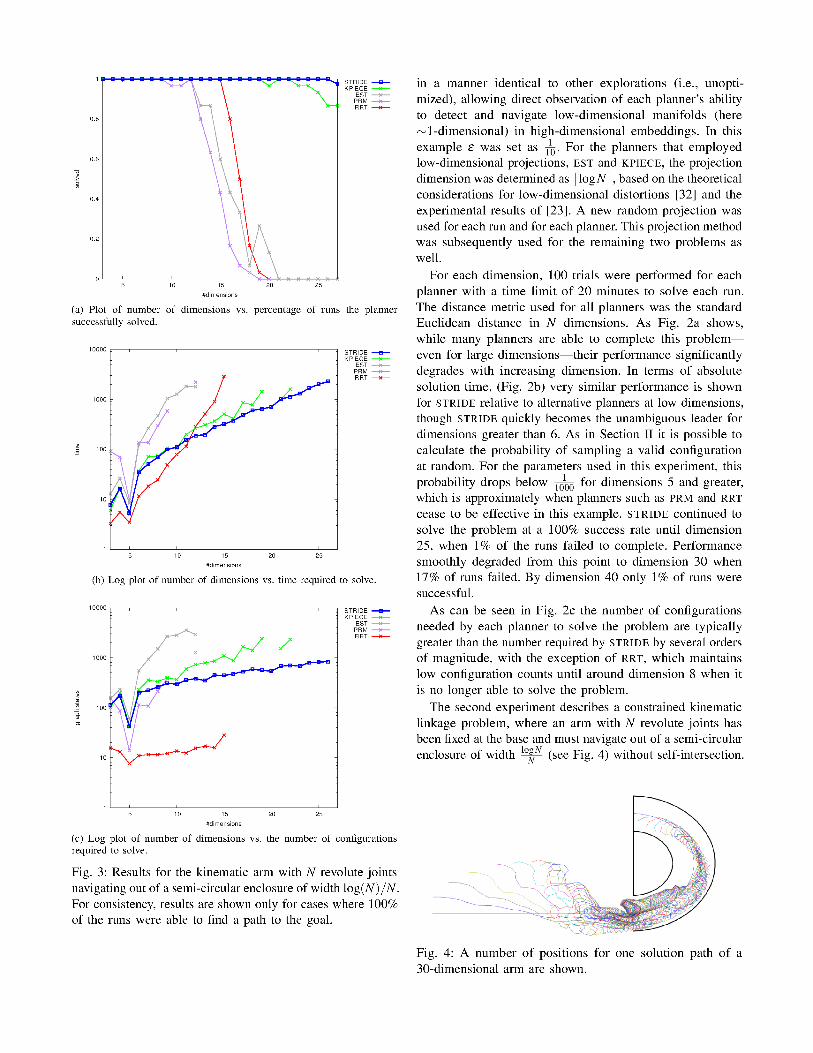
(c) Log plot showing number of dimensions vs. the number of configurationsrequired to solve.

Fig. 2: Results for the Hyper Cube problem. For consistency,

results are shown only for cases where 100% of the runs

were able to find a path to the goal.

defined implicitly by a validState function (see Algorithm 1),

the planners were required to explore this simple space

The value of N was allowed to vary from 3 to 27 dimensions,

with experiments run for a maximum of 2 hours, 30 times

each for the above listed planners. In this case, the metric used

for all planners was the summed Euclidean joint distance [1],

defined by ∑ ||ai −bi|| with ai and bi representing the vector

position of the ith joint in configurations a and b, respectively,

in the kinematic chain.

As seen in Fig. 3b, STRIDE provides solidly average

performance in the 2–6 dimension range, when compared

against other planners, with RRT the clear winner for this

range and KPIECE as competitive. From dimension 6–10

STRIDE begins to outperform KPIECE, with RRT still the

unambiguous leader. From dimension 11–20 STRIDE becomes

the clear winner, with many planners occasionally failing to

complete past about 12 dimensions. Only with 27 joints did

STRIDE begin to have difficulty solving the problem within

2 hours, with 1 of the 30 runs failing to complete the task.

Further, Fig. 3c shows that for dimensions greater than 10

STRIDE produced, on average, less than half of the number

of configurations required by other planners.

The last problem applies the above planners to the classic

“piano mover’s problem” in which a rigid body must move

through a constrained environment between a start and goal

position. In this experiment, a studio piano was required to

move through a relatively constrained apartment environment

(see Fig. 5). Due to several sharp corners, tight coupling

between rotational and spatial degrees of freedom in this

problem was required, producing a 6-dimensional problem

with several distinct lower-dimensional narrow passages. Here,

20 experiments were run for each planner with a time limit

of 1000 seconds each. For all planners in this experiment, the

metric was defined as the unweighted sum of the Euclidean

distance between the centroids of configurations and the arc-

length between their respective rotations (as in [33]).

In this example STRIDE still outperforms alternative plan-

Fig. 5: A piano is moved through a highly-constrained

apartment environment. Red dots indicate the center of

the piano for a number of sampled configurations. A few

configurations of a solution path are overlaid.

TABLE I: Table of average solution times and average number

of configurations generated for each planner for the piano-

mover’s problem. All values represent averages over 20 runs

limited to a maximum runtime of 1000 seconds each.

Planner Time States

STRIDE 85.77 9525.45

EST 107.54 30314.85

RRT 443.96 152669.45

KPIECE 1 521.34 655003.45

PRM 685.62 83650.85

ners, although by a slimmer margin (see Table I) Additionally,

STRIDE also produces nearly an order of magnitude fewer

configurations than the next best planner, EST.

The piano-movers problem was performed on a quad core

2.8 GHz Intel Core i5 CPU 760 and a total of 8GB of RAM.

All other experiments were performed on a cluster with two

quad core 2.4 GHz Intel Xeon (Nehalem) CPUs with 12GB

of RAM per node.

V. CONCLUSIONS

We have presented a novel planner, STRIDE, for motion

planning which takes advantage of the GNAT data-structure

allowing for a completely abstract, resolution-independent,

density estimation heuristic. In the examples presented, we

have demonstrated that STRIDE produces a smoothly varying,

predictable response to an increase in dimension, both in

time and memory used. Unlike other specialized planners,

STRIDE is largely parameter-free, requiring only a suitably

defined distance metric for the system under consideration

and an optional estimation of the dimension of the free

space. Sampling is performed recursively, resulting in natural,

resolution-independent, density estimation that leads to an

uniform sampling of a full space, with preference given to low-

density boundary regions. The GNAT data structure was chosen

for generality and efficiency across the broadest possible

definitions of configuration space, including non-Euclidean

spaces. However, nothing in the preceding argument would

preclude the use of an alternative, tree-based nearest-neighbor

data structure (e.g., K-D trees [34]) for determining sampling

density in spaces where their construction or accuracy of

estimation of density is superior to a GNAT. Extension and

comparison to alternative nearest neighbor data structures is

left for future work.

This version of STRIDE is closest to the EST planner in

structure, using a novel heuristic and sampling scheme. In

particular, each node was assumed to be approximately an

N-sphere in the dimension of the space, an assumption that

is almost certainly inaccurate for most spaces. Improved

methods for the estimation of the density of Voronoi cells

would likely provide the greatest improvement to the planner

as a whole, as exploration is performed relative to this alone,

and is left for future work. The ability of planners such

as KPIECE to determine the “edges” of sampled regions

using “boundary cells”, allows them to rapidly expand into

unexplored regions by preferentially sampling boundary re-

gions. While bounded or periodic metric spaces (e.g. toroidal,

spherical) may not have a natural notion of “boundary”,

an extension or abstraction of this concept to determine

Voronoi cells with a large number of empty neighbors for

biasing would likely make STRIDE more competitive in

low-dimensional/Euclidean spaces, though this is left for

future work. As described earlier, another natural extension

of the planner presented here would be bi-directional form

of STRIDE. Finally, generalizing this planner to kinodynamic

systems remains a goal left for future work.

VI. ACKNOWLEDGMENTS

This work has been supported in part by The Texas Higher

Education Coordinating Board (NHARP 01907), The John

and Ann Doerr Fund for Computational Biomedicine at Rice

University, NSF DUE 0920721, NSF CCF 1018798, and Rice

University funds. BG is also supported in part by a training

fellowship from the Keck Center NLM Training Program in

Biomedical Informatics of the Gulf Coast Consortia (NLM

Grant No. T15LM007093). Experiments were run on (i)

equipment of the Shared University Grid at Rice funded by

NSF under Grant EIA-0216467, and a partnership between

Rice University, Sun Microsystems, and Sigma Solutions, Inc.,

and (ii) equipment funded by NSF CNS-0821727 and by NIH

award NCRR S10RR02950 and an IBM Shared University

Research (SUR) Award in partnership with CISCO, Qlogic

and Adaptive Computing.

REFERENCES

[1] J.-C. Latombe, Robot Motion Planning. Boston, MA: KluwerAcademic Publishers, Dec. 1990.

[2] N. Haspel, M. Moll, M. L. Baker, W. Chiu, and L. E. Kavraki, “Tracingconformational changes in proteins.” BMC structural biology, vol. 10Suppl 1, p. S1, 2010.

[3] L. Tapia, S. Thomas, and N. M. Amato, “A motion planning approachto studying molecular motions,” Commun. Inf. Syst., vol. 10, no. 1, pp.53–68, 2010.

[4] J. Cortes, T. Simeon, V. Ruiz de Angulo, D. Guieysse, M. Remaud-Simeon, and V. Tran, “A path planning approach for computing large-amplitude motions of flexible molecules.” Bioinformatics, vol. 21 Suppl1, pp. i116–25, 2005.

[5] M. Lau and J. J. Kuffner, “Behavior planning for character animation,”in Proc. ACM SIGGRAPH/Eurographics Symposium on Computer

animation, New York, NY, USA, 2005, pp. 271–280.[6] A. Bhatia, L. Kavraki, and M. Vardi, “Sampling-based motion planning

with temporal goals,” in IEEE International Conference on Robotics

and Automation (ICRA), 2010. Proceedings., 2010, May 2010, pp.2689–2696.

[7] A. Bhatia, M. Maly, L. E. Kavraki, and M. Y. Vardi, “Motion planningwith complex goals,” Robotics Automation Magazine, IEEE, vol. 18,no. 3, pp. 55–64, sept. 2011.

[8] H. Choset, K. Lynch, S. Hutchinson, G. Kantor, W. Burgard, L. E.Kavraki, and S. Thrun, Principles of Robot Motion Theory, Algorithms,

and Implementation. Cambridge: MIT Press, 2005.[9] S. M. LaValle, Planning Algorithms. Cambridge University Press,

May 2006.[10] L. Kavraki, P. Svestka, J.-C. Latombe, and M. Overmars, “Probabilistic

roadmaps for path planning in high-dimensional configuration spaces,”IEEE Transactions on Robotics and Automation, vol. 12, no. 4, pp.566–580, Aug. 1996.

[11] S. M. LaValle and J. J. Kuffner, “Randomized kinodynamic planning,”The International Journal of Robotics Research, vol. 20, no. 5, pp.378–400, May 2001.

[12] D. Hsu, J.-C. Latombe, and R. Motwani, “Path planning in expan-sive configuration spaces,” Intl. J. of Computational Geometry and

Applications, vol. 9, no. 4-5, pp. 495–512, 1999.[13] G. Sanchez and J.-C. Latombe, “On delaying collision checking in PRM

planning: Application to multi-robot coordination,” The International

Journal of Robotics Research, vol. 21, no. 1, pp. 5–26, 2002.[14] N. M. Amato and G. Song, “Using motion planning to study protein

folding pathways,” Journal of Computational Biology, vol. 9, no. 2,pp. 149–168, Apr. 2002.

[15] N. M. Amato, O. B. Bayazit, L. K. Dale, C. Jones, and D. Vallejo,“OBPRM: an obstacle-based PRM for 3D workspaces,” in Workshop

on Algorithmic Foundations of Robotics, 1998, pp. 155–168.[16] V. Boor, M. H. Overmars, and A. F. van der Stappen, “The Gaus-

sian sampling strategy for probabilistic roadmap planners,” in IEEE

International Conference on Robotics and Automation (ICRA), 1999.

Proceedings., 1999, 1999, pp. 1018–1023.[17] L. J. Guibas, C. Holleman, and L. E. Kavraki, “A probabilistic

roadmap planner for flexible objects with a workspace medial-axis-based sampling approach,” in Proc. IEEE/RSJ Intl. Conf. on Intelligent

Robots and Systems, vol. 1, 1999, pp. 254–259.[18] T. Simeon, J.-P. Laumond, and C. Nissoux, “Visibility-based proba-

bilistic roadmaps for motion planning,” Advanced Robotics, vol. 14,no. 6, pp. 477–493, 2000.

[19] M. Kobilarov, “Cross-entropy motion planning,” The International

Journal of Robotics Research, vol. 31, no. 7, pp. 855–871, June 2012.[20] S. Kumar and S. Chakravorty, “Adaptive sampling for generalized

probabilistic roadmaps,” Journal of Control Theory and Applications,vol. 10, no. 1, pp. 1–10, 2012.

[21] J. Pan, S. Chitta, and D. Manocha, “Faster sample-based motionplanning using instance-based learning,” in Proc. Workshop on the

Algorithmic Foundations of Robotics, 2012.[22] I. A. Sucan and L. E. Kavraki, “A sampling-based tree planner for

systems with complex dynamics,” IEEE Transactions on Robotics,vol. 28, no. 1, pp. 116–131, 2012.

[23] I. A. Sucan and L. E. Kavraki, “On the performance of randomlinear projections for sampling-based motion planning,” in IEEE/RSJ

International Conference on Intelligent Robots and Systems, 2009.

IROS 2009., 2009, pp. 2434–2439.[24] I. A. Sucan, M. Moll, and L. E. Kavraki, “The Open Motion Planning

Library,” IEEE Robotics & Automation Magazine, vol. 19, no. 4, pp.72–82, December 2012, http://ompl.kavrakilab.org.

[25] S. Dalibard and J.-P. Laumond, “Linear dimensionality reductionin random motion planning,” The International Journal of Robotics

Research, vol. 30, no. 12, pp. 1461–1476, Oct. 2011.[26] A. M. Ladd and L. E. Kavraki, “Motion planning in the presence of

drift, underactuation and discrete system changes,” in Robotics: Science

and Systems I. Boston, MA: MIT Press, 2005, pp. 233–241.[27] E. Plaku, L. Kavraki, and M. Vardi, “Motion planning with dynamics

by a synergistic combination of layers of planning,” IEEE Trans. on

Robotics, vol. 26, no. 3, pp. 469–482, jun. 2010.[28] Q. Sajid, R. Luna, and K. E. Bekris, “Multi-agent pathfinding with

simultaneous execution of single-agent primitives,” in Fifth Symposium

on Combinatorial Search (SoCS), Niagara Falls, CA, July 19-21 2012.[29] S. Brin, “Near neighbor search in large metric spaces,” in Proc. 21st

Conf. on Very Large Databases, 1995, pp. 574–584.[30] T. F. Gonzalez, “Clustering to minimize the maximum intercluster

distance,” Theoretical Computer Science, vol. 38, pp. 293–306, 1985.[31] A. Shkolnik and R. Tedrake, “Path planning in 1000+ dimensions

using a task-space Voronoi bias,” in IEEE International Conference on

Robotics and Automation (ICRA), 2009. Proceedings., 2009. IEEE,May 2009, pp. 2061–2067.

[32] W. B. Johnson and J. Lindenstrauss, “Extensions of Lipschitz mappingsinto a Hilbert space,” Contemporaty Mathematics, vol. 26, pp. 189–206,1984.

[33] J. J. Kuffner, “Effective sampling and distance metrics for 3D rigidbody path planning,” in IEEE International Conference on Robotics and

Automation (ICRA), 2004. Proceedings., 2004, 2004, pp. 3993–3998.[34] J. L. Bentley, “Multidimensional binary search trees used for associative

searching,” Communications of the ACM, vol. 18, no. 9, pp. 509–517,Sept. 1975.