resistance vs. load reliability analysis

Resistance vs. Load Reliability Analysis

Let L be the load acting on a system (e.g. footing) andlet R be the resistance (e.g. soil)

Then we are interested in controlling R such that the probabilitythat R > L (i.e. the reliability) is acceptably high or, equivalently,that R < L (i.e. the failure probability) is acceptably low, where

[ ]P ( , )RLr l

R L f r l drdl∞ ∞

−∞ <

< = ∫ ∫and where is the joint (bivariate) distribution of R and L.( , )RLf r l

[ ]( , ) PRLf r l dr dl r R r dr l L l dl= < ≤ + < ≤ +∩

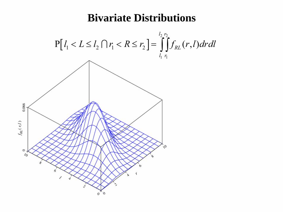
Bivariate Distributions

[ ]2 2

1 1

1 2 1 2P ( , )l r

RLl r

l L l r R r f r l drdl< ≤ < ≤ = ∫ ∫∩


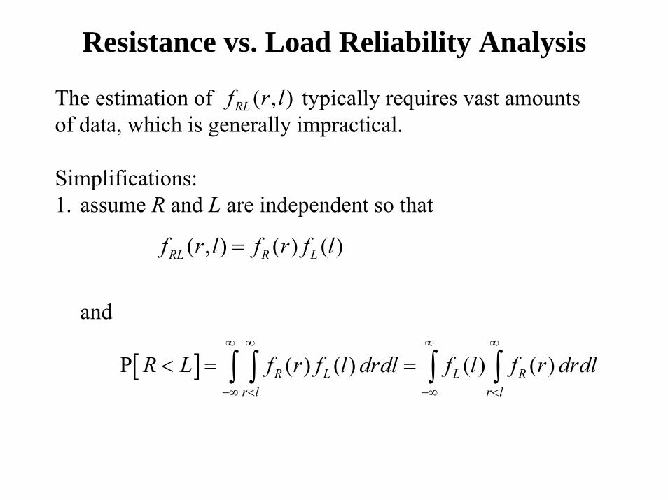
The estimation of typically requires vast amountsof data, which is generally impractical.

Simplifications:1. assume R and L are independent so that

and

( , )RLf r l

( , ) ( ) ( )RL R Lf r l f r f l=

[ ]P ( ) ( ) ( ) ( )R L L Rr l r l

R L f r f l drdl f l f r drdl∞ ∞ ∞ ∞

−∞ < −∞ <

< = =∫ ∫ ∫ ∫


2. Assume R and L are either normally or lognormallydistributed.The event {R < L} is the same as the events

i) {R – L < 0}ii) {R/L < 1}

If both R and L are normally distributed, thenX R L= −

is also normally distributed with parameters

(assuming R and L are independent).

2 2 2X R L

X R L

μ μ μ

σ σ σ

= −

= +

Reliability Index

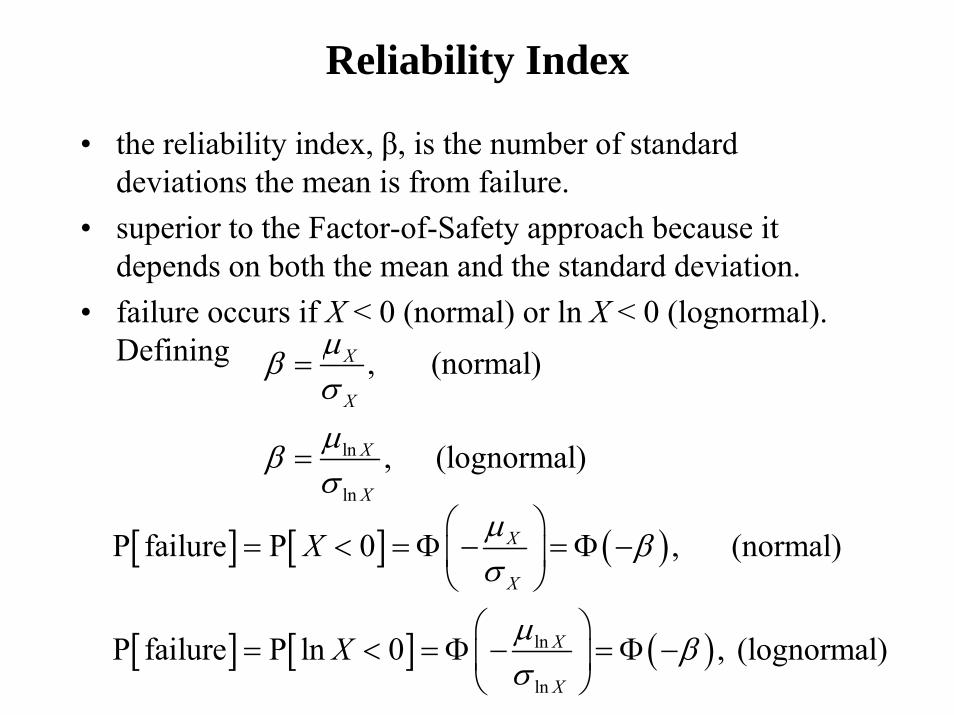
• the reliability index, β, is the number of standard deviations the mean is from failure.

• superior to the Factor-of-Safety approach because it depends on both the mean and the standard deviation.

• failure occurs if X < 0 (normal) or ln X < 0 (lognormal).Defining

ln

ln

, (normal)

, (lognormal)

X

X

X

X

μβσμβσ

=

=

[ ] [ ] ( )

[ ] [ ] ( )ln

ln

P failure P 0 , (normal)

P failure P ln 0 , (lognormal)

X

X

X

X

X

X

μ βσ

μ βσ

⎛ ⎞= < = Φ − = Φ −⎜ ⎟

⎝ ⎠⎛ ⎞

= < = Φ − = Φ −⎜ ⎟⎝ ⎠


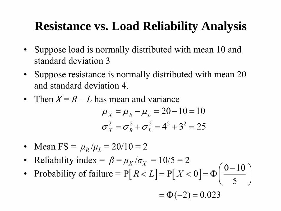
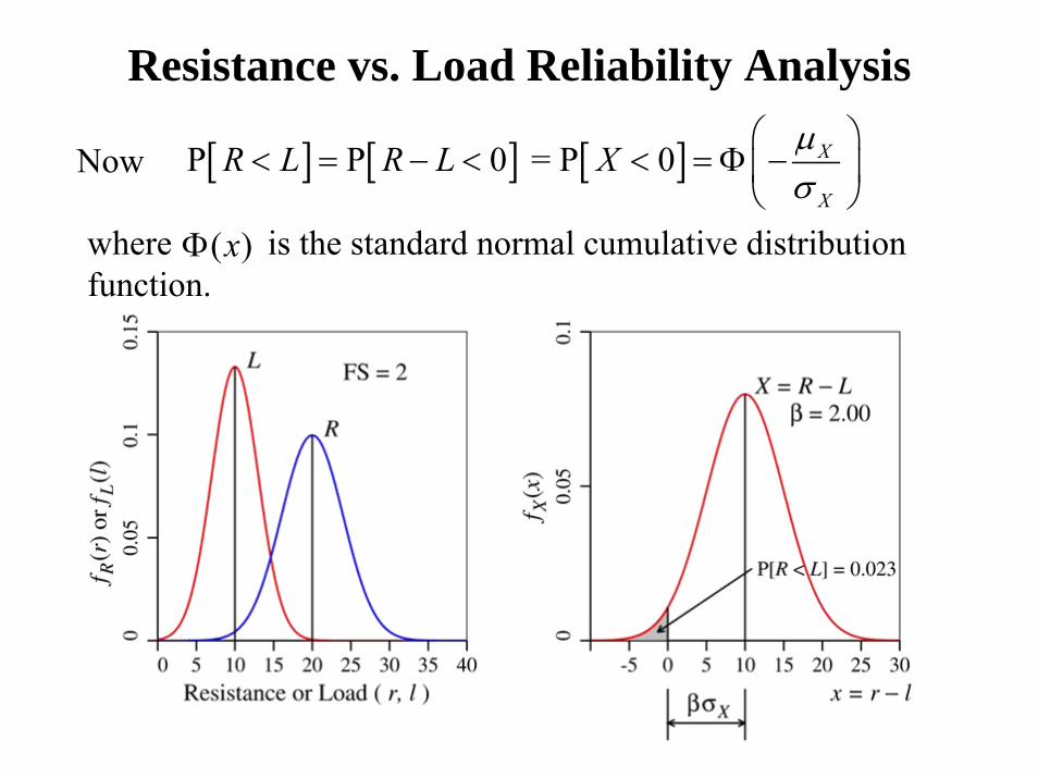
• Suppose load is normally distributed with mean 10 and standard deviation 3

• Suppose resistance is normally distributed with mean 20 and standard deviation 4.

• Then X = R – L has mean and variance

• Mean FS = μR /μL = 20/10 = 2• Reliability index = β = μX /σX = 10/5 = 2• Probability of failure =

2 2 2 2 2

20 10 10

4 3 25X R L

X R L

μ μ μ

σ σ σ

= − = − =

= + = + =

[ ] [ ] 0 10P P 05

( 2) 0.023

R L X −⎛ ⎞< = < = Φ⎜ ⎟⎝ ⎠

= Φ − =


Now [ ] [ ] [ ]P P 0 = P 0 X

X

R L R L X μσ

⎛ ⎞< = − < < = Φ −⎜ ⎟

⎝ ⎠where is the standard normal cumulative distributionfunction.

( )xΦ


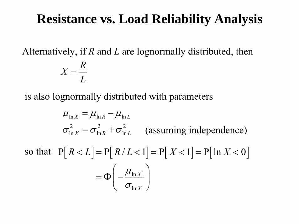
Alternatively, if R and L are lognormally distributed, thenRXL

=

is also lognormally distributed with parameters

ln ln ln2 2 2ln ln ln

X R L

X R L

μ μ μ

σ σ σ

= −

= + (assuming independence)

so that [ ] [ ] [ ] [ ]ln

ln

P P / 1 P 1 P ln 0

X

X

R L R L X X

μσ

< = < = < = <

⎛ ⎞= Φ −⎜ ⎟

⎝ ⎠


• Suppose load is lognormally distributed with mean 10 and standard deviation 3

• Suppose resistance is lognormally distributed with mean 20 and standard deviation 4.

• Then X = R/L is lognormally distributed

20, 4R Rμ σ= = →( )

22ln 2

2ln ln

ln 1 0.0392

ln 0.5 2.976

RR

R

R R R

σσμ

μ μ σ

⎛ ⎞= + =⎜ ⎟

⎝ ⎠= − =

10, 3L Lμ σ= = →( )

22ln 2

2ln ln

ln 1 0.0862

ln 0.5 2.259

LL

L

L L L

σσμ

μ μ σ

⎛ ⎞= + =⎜ ⎟

⎝ ⎠= − =

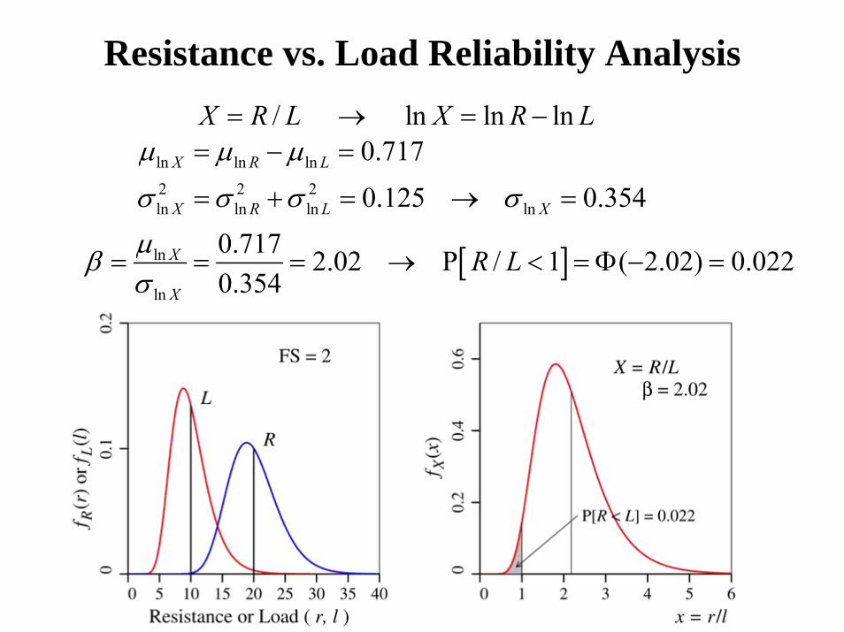
Resistance vs. Load Reliability Analysis/ ln ln lnX R L X R L= → = −

ln ln ln2 2 2ln ln ln ln

0.717

0.125 0.354X R L

X R L X

μ μ μ

σ σ σ σ

= − =

= + = → =

[ ]ln

ln

0.717 2.02 P / 1 ( 2.02) 0.0220.354

X

X

R Lμβσ

= = = → < = Φ − =

Reliability Index

Reliability Index

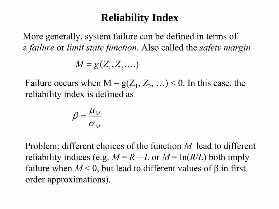
More generally, system failure can be defined in terms ofa failure or limit state function. Also called the safety margin

1 2( , , )M g Z Z= …

Failure occurs when M = g(Z1, Z2, …) < 0. In this case, thereliability index is defined as

M

M

μβσ

=

Problem: different choices of the function M lead to differentreliability indices (e.g. M = R – L or M = ln(R/L) both implyfailure when M < 0, but lead to different values of β in firstorder approximations).

Reliability IndexExample 1: suppose that M = R – Land R and L are normally distributed. Then

2 2 (assuming independence)M R L

M R L

μ μ μ

σ σ σ

= −

= +and

so that2 2

R L

R L

μ μβσ σ

−=

+

and [ ] [ ] ( )P failure P 0M β= < = Φ −

This is exact, so long as R and L are normally distributedand independent (if not independent then must involvecovariances in computation of σM).

Reliability IndexExample 2: suppose that M = ln( R / L ) = lnR – lnLand R and L are lognormally distributed. Then

ln ln

2 2ln ln (assuming independence)

M R L

M R L

μ μ μ

σ σ σ

= −

= +and

so that ln ln2 2ln ln

R L

R L

μ μβσ σ

−=

+

and [ ] [ ] ( )P failure P 0M β= < = Φ −

This is exact, so long as R and L are lognormally distributedand independent (if not independent then must involvecovariances in computation of σM).

Reliability IndexExample 3: suppose that M = ln( R / L ) = lnR – lnLand R and L are normally distributed. Then the distributionof M is complex and we must approximate its moments;

2 22 2ln ln

2 22 2

2 2

ln ln (to first order)

=

R L

M R L

M R L

R LR L

R L

M MR L

V V

μ μ

μ μ μ

σ σ σ

σ σμ μ

−

∂ ∂⎛ ⎞ ⎛ ⎞+⎜ ⎟ ⎜ ⎟∂ ∂⎝ ⎠ ⎝ ⎠

+ = +

2 2R L

R L

μ μβσ σ

−=

+now

2 2

ln lnR L

R LV Vμ μβ −

=+

It was

These are clearly different.

in Example 1

Hasover-Lind Reliability Index

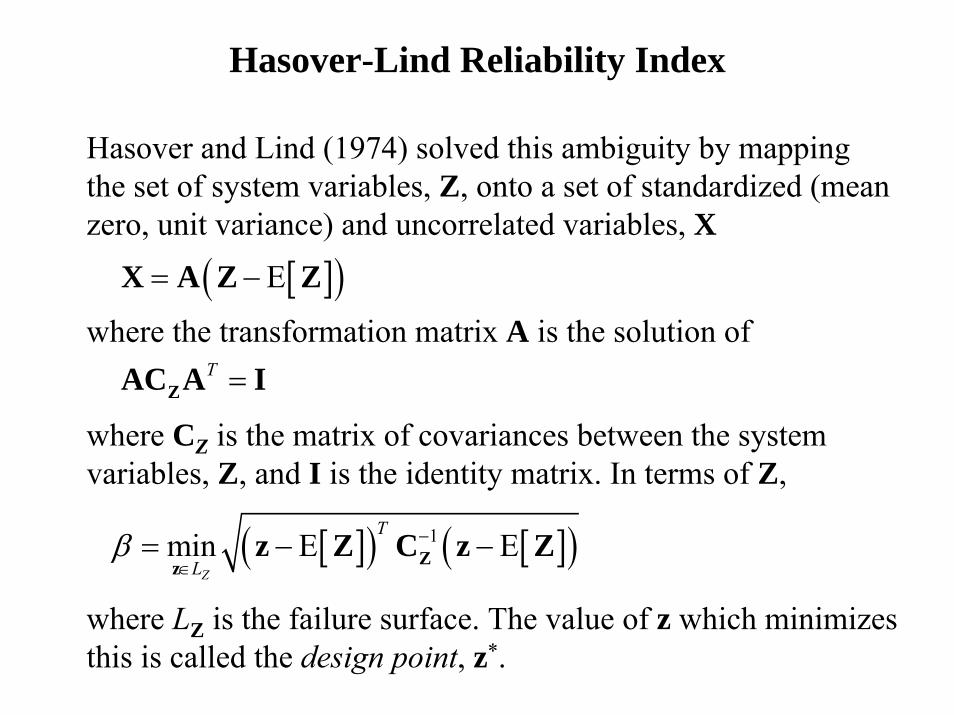
Hasover and Lind (1974) solved this ambiguity by mappingthe set of system variables, Z, onto a set of standardized (meanzero, unit variance) and uncorrelated variables, X

[ ]( )E= −X A Z Z

where the transformation matrix A is the solution ofT =ZAC A I

where CZ is the matrix of covariances between the systemvariables, Z, and I is the identity matrix. In terms of Z,

[ ]( ) [ ]( )1min E EZ

T

Lβ −

∈= − −Zz

z Z C z Z

where LZ is the failure surface. The value of z which minimizesthis is called the design point, z*.

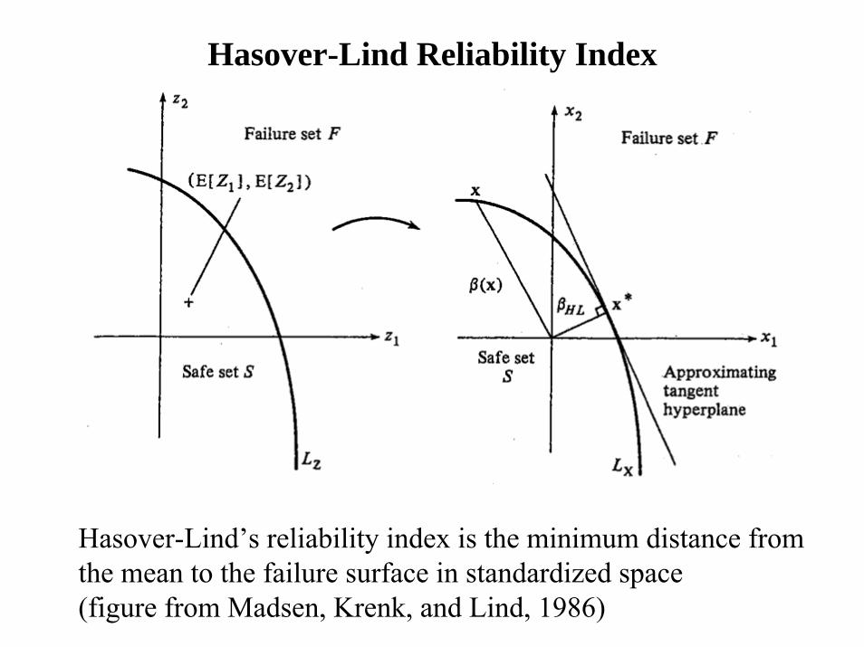
Hasover-Lind Reliability Index

Hasover-Lind’s reliability index is the minimum distance fromthe mean to the failure surface in standardized space(figure from Madsen, Krenk, and Lind, 1986)

Going Beyond Calibration• Must move beyond calibration for real benefits of LRFD• Simple probability-based methods take load and

resistance distributions into account- nominal or characteristic resistance: Rn = kRμR- nominal or characteristic load: Ln = kLμL

• Design: ϕ Rn = γ Ln

P[failure] P[ ] P[ / 1]R L R L= < = <

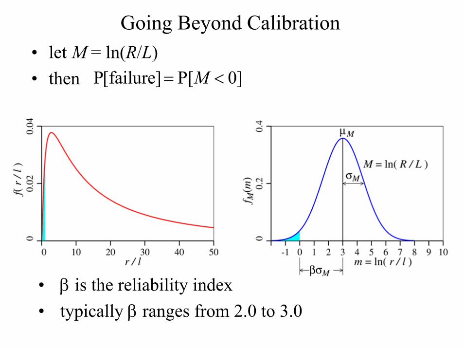
• let M = ln(R/L)• then P[failure] P[ 0]M= <

• β is the reliability index• typically β ranges from 2.0 to 3.0

Going Beyond Calibration

We want to produce a design such that the mean and standard deviation ofresistance satisfies

[ ]P 1 P ln ln 0 ( )R R LL

β⎡ ⎤< = − < = Φ −⎢ ⎥⎣ ⎦

In detailln ln

2 2ln ln

0 E[ln ln ]P[ln ln 0] P ( )SD[ln ln ]

R L

R L

R LR L ZR L

μ μ βσ σ

⎛ ⎞⎡ ⎤ −− − ⎜ ⎟− < = < = Φ − = Φ −⎢ ⎥ ⎜ ⎟−⎣ ⎦ +⎝ ⎠so that2ln ln

ln ln ln ln2 2ln ln

R LR L R L

R L

μ μ β μ μ β σ σσ σ

−= ⇒ = + +

+ln ln ln0.75 ( )L R Lμ β σ σ+ +

Now, since 2ln lnln( ) 0.5L L Lμ μ σ= − and ( )2

ln lnexp 0.5R Rμ μ σ= + Rwe get

To determine both load and resistance factors:

{ } { }2 2ln ln ln lnexp 0.5 0.75 exp 0.5 0.75R L R R L Rμ μ σ βσ σ βσ⎡ ⎤= + − +⎣ ⎦

or

{ } { }2 2ln ln ln lnexp 0.5 0.75 exp 0.5 0.75R R R L R Lσ βσ μ σ βσ μ+ = − +

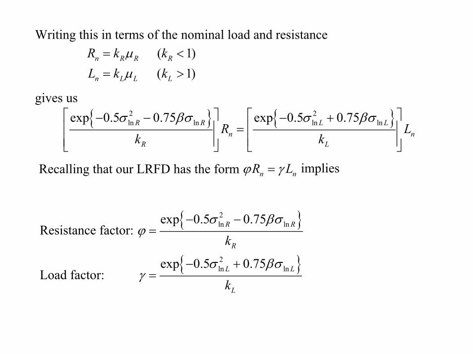
Writing this in terms of the nominal load and resistance ( 1) ( 1)

n R R R

n L L L

R k kL k k

μμ

= <

= >

gives us{ } { }2 2

ln ln ln lnexp 0.5 0.75 exp 0.5 0.75R R L Ln n

R L

R Lk k

σ βσ σ βσ⎡ ⎤ ⎡ ⎤− − − +⎢ ⎥ ⎢ ⎥=⎢ ⎥ ⎢ ⎥⎣ ⎦ ⎣ ⎦

Recalling that our LRFD has the form n nR Lϕ γ= implies

Resistance factor:{ }

{ }

2ln ln

2ln ln

exp 0.5 0.75

exp 0.5 0.75

R R

R

L L

L

k

k

σ βσϕ

σ βσγ

− −=

− +=Load factor:

If load factors are known (e.g. from structural codes) then the resistancefactor becomes dependent on both the resistance variability and theload variability. In this case, our LRFD can be written

i i

i

i n i ni i

n i ni n R R

L LR L

R k

γ γϕ γ ϕ

μ= ⇒ = =

∑ ∑∑

{ }2

2 2ln ln2

1exp

1

ii nLi

R LR L R

Q Vk V

γβ σ σ

μ

⎛ ⎞+⎜ ⎟= − +⎜ ⎟+⎝ ⎠

∑

wherei i in L LL k μ=

i

i

i

nL L

i i L

Lk

μ μ= =∑ ∑2 2i iL LiL

LL L

VV

μσμ μ

= =∑ (assuming loads are independent)

Going Beyond Calibration

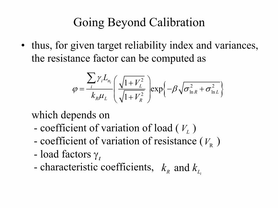
• thus, for given target reliability index and variances, the resistance factor can be computed as

which depends on- coefficient of variation of load ( )- coefficient of variation of resistance ( )- load factors γι- characteristic coefficients,

LV

RV

and iR Lk k

{ }2

2 2ln ln2

1exp

1

ii nLi

R LR L R

L Vk V

γϕ β σ σ

μ

⎛ ⎞+⎜ ⎟= − +⎜ ⎟+⎝ ⎠

∑

Problems Implementing LRFD

• the coefficient of variation of resistance depends on;- variability in material properties- error in design models- measurement and correlation errors- construction variability

• with steel and concrete, the material property variability does not change significantly with location (quality controlled materials)

• with soils, the material property mean and variability change within a site and from site to site


• there is a dependence between resistance and load which is generally absent (or small) in structural engineering, e.g. shear strength is dependent on stress;

tanf cτ σ φ= +


• No common definition of “characteristic value”- often defined as a “cautious estimate of the

mean”, but sometimes as a low percentile- we badly need a standard definition (median?)

• VR changes with intensity of site investigation- resistance factor should approach 1.0 as the

site is more thoroughly investigated- this would lead to a complex table of resistance

factors (however, see, e.g., AS 5100, AS 2159,AS4678, Eurocode 7, NCHRP507)

Future Directions

• probabilistic methods generally limited to “single random variable” models (e.g. R vs. L)

• to consider the effect of spatial variability, random field simulation combined with finite element analysis is necessary (RFEM)

• the random field simulation allows the representation of a soil’s spatial variability

• the finite element analysis allows the soil to fail along “weakest paths” (decreased model error)

Conclusions

• geotechnical engineers led the way with Limit States concepts (1940’s) but have been slow to migrate to reliability-based design methods.

• the most advanced LRFD codes currently are AS 5100 and Eurocode 7.

• all current LRFD geotechnical codes have load and resistance factors calibrated from older WSD codes, with some adjustments based on engineering judgement and simple probability methods.

resistance vs. load reliability analysis

Documents