residual generator fuzzy identification for automotive...

Int. J. Appl. Math. Comput. Sci., 2013, Vol. 23, No. 2, 419–438DOI: 10.2478/amcs-2013-0032

RESIDUAL GENERATOR FUZZY IDENTIFICATION FOR AUTOMOTIVEDIESEL ENGINE FAULT DIAGNOSIS

SILVIO SIMANI

Department of EngineeringUniversity of Ferrara, Via Saragat 1E, 44124 Ferrara (FE), Italy

e-mail: [email protected]

Safety in dynamic processes is a concern of rising importance, especially if people would be endangered by serious systemfailure. Moreover, as the control devices which are now exploited to improve the overall performance of processes includeboth sophisticated control strategies and complex hardware (input-output sensors, actuators, components and processingunits), there is an increased probability of faults. As a direct consequence of this, automatic supervision systems shouldbe taken into account to diagnose malfunctions as early as possible. One of the most promising methods for solving thisproblem relies on the analytical redundancy approach, in which residual signals are generated. If a fault occurs, theseresidual signals are used to diagnose the malfunction. This paper is focused on fuzzy identification oriented to the designof a bank of fuzzy estimators for fault detection and isolation. The problem is treated in its different aspects covering themodel structure, the parameter identification method, the residual generation technique, and the fault diagnosis strategy.The case study of a real diesel engine is considered in order to demonstrate the effectiveness the proposed methodology.

Keywords: fault detection and isolation, analytical redundancy, Takagi–Sugeno fuzzy prototypes, residual generator fuzzymodelling and identification, real diesel engine.

1. Introduction

The control devices currently in use to improve theoverall performance of industrial processes involve bothsophisticated digital control techniques and complexhardware (sensors, actuators and processing units). Thecomplexity means that the probability of fault occurrencecan be significant and an automatic supervisory controlsystem should be used to detect and isolate anomalousworking conditions as early as possible. Thesemotivations pushed great attention on Fault Detection andIsolation (FDI) in dynamic processes and a wide variety ofapproaches have been proposed (Chen and Patton, 1999;Isermann, 2005; Simani et al., 2003; Ding, 2008). Theyare based, e.g., on the parity space, state estimation,Unknown Input Observers (UIOs), Kalman Filters (KFs),Unknown Input Kalman Filters (UIKFs), and parameteridentification. On the other hand, artificial intelligencetechniques can be also exploited (Korbicz et al., 2004).Although many linear and nonlinear approaches havebeen developed, robust and reliable FDI for dynamicprocesses is still a problem open to further research.

In order to guarantee that faults can be detectedand isolated (and distinguishable), accurate mathematical

models of the process under investigation are required, ineither the state space or input-output forms. Residualsshould then be processed to detect an actual faultcondition, rejecting any false alarms caused by noiseor spurious signals. However, in practical situations,the straightforward application of model-based FDItechniques can be difficult, due to dynamic modelcomplexity. In fact, the plant analytical description isusually designed to carefully capture all kinds of detailsrelevant to the analysis and deployment of the real system.On the other hand, this intrinsic complexity makes theuse of many cited linear FDI methods, almost infeasibleand a viable procedure for practical application of FDItechniques is really necessary in practical cases (Chen andPatton, 1999; Simani et al., 2003).

In particular, many papers on model-based FDIwere published over the last decade, using both signal-and process model-based methods (Svard-Nyberg, 2010a;2010b; Jain et al., 2012; Marusak and Tatjewski, 2008).Unsurprisingly, these show that the more accurate themodel is at describing the engine behaviour, the better itsperformance will be in detecting anomalous conditions.Unfortunately, an accurate and complete mathematical

[email protected]

420 S. Simani

model of such a complex thermodynamic system isusually unavailable, typically because of the assumptionsintroduced to reduce mathematical complexity. Hence,FDI schemes that relate to first principle engine modelsare costly to develop, while current alternatives tend to bemathematically complex or require considerable a prioriknowledge to be incorporated into the monitoring scheme.

In this paper, the use of fuzzy identification isproposed through a real process for finding a viablesolution to the FDI problem. To this end, two practicalaspects of the presented work are stressed. Firstly, thesystem complexity may not indicate a requirement for asophisticated physical or thermodynamic model. In fact,as shown in this work, a fuzzy identification method canbe successfully used, thus obviating the requirement forphysical models. In particular, the Errors-In-Variables(EIV) framework (Van Huffel and Lemmerling, 2002) anda proper identification algorithm are used in connectionwith fuzzy logic descriptions. Secondly, fuzzy prototypesfor residual generation are considered instead of usingpurely nonlinear observers or filters. Moreover, as thepurpose of system supervision is to monitor the conditionsof the system at different working points, piecewise affineprototypes are successfully proposed. Real data from adiesel engine are considered.

This paper suggests to use fuzzy system theory, sinceit seems to be a natural tool to handle complicated anduncertain processes, such as diesel engines. Thus, itis suggested to exploit residual generators in the formof Takagi–Sugeno (TS) fuzzy prototypes (Takagi andSugeno, 1985), whose parameters are easily obtained byidentification procedures. It should finally be pointedout how the fuzzy approach can solve the problem attwo levels. First, fuzzy TS models are used to generateresidual signals for fault detection. Second, fault isolationis achieved using again the identified fuzzy TS prototypesorganised into a bank structure.

Finally, the effectiveness of the proposedidentification and fault diagnosis strategies is assessedon real data sequences acquired from full Europeandriving cycle tests. Realistic fault conditions anddifferent working situations have been considered, inorder to provide an accurate validation of the proposedmethodology. The main features of the diagnosisapproach suggested in this paper are compared withdifferent schemes based, e.g., on a UIO/KF bank.

The paper has the following structure. Section 2briefly recalls the structure of the diesel engine. Section 4addresses the fuzzy identification strategy exploited forobtaining the residual generators which will be usedfor the design of the fault diagnosis strategy. Thisdiagnosis methodology is presented in Section 5. Theachieved results summarised in Section 6 show theperformances of the diagnosis schemes, validated onreal data directly acquired from the diesel engine, and

compared also with a different fault diagnosis strategy.Finally, Section 7 concludes the paper by highlighting themain achievements of the work.

2. Diesel engine system

Section 3 provides brief details regarding the dieselengine considered in this work, which was designedby the company VM Motors S.p.A. in connection withthe embedded controller developed by BOSCH (Bosch,2006). Section 3.1 illustrates the faults of interest for VMMotors S.p.A., which will be diagnosed by the suggestedFDI scheme.

3. Controlled turbocharged engine

In this work, a diesel engine “Panther” RA428 equippedwith a fixed geometry turbine, an external ExhaustGas Recirculation (EGR) system, and a Throttle ValveActuator (TVA) is considered, as shown in Fig. 1.

Diesel EngineEGR Valve

TVA Valve

TurbineCompressor

Intercooler

Exhaust

Manifold

Intake

Manifold

Fig. 1. Diesel engine air system.

This in-line 4 cylinder (2.8 l.) diesel motor isproduced by VM Motors S.p.A. (Cento, Ferrara, Italy),but its engine is used in JK Jeep Wrangler outside of theUS market. This engine main features are

• 2776 cc of displacement,

• 4 valve/per cylinder,

• Double Over Head Camshaft (DOHC),

• BOSCH common rail direct injection with electricpiezo injectors operating at 30,000 psi,

• weight of 451 pounds / 205 kg, power rating of 174horsepower, 340 foot pounds.

In the following, the basics of the diesel engine physicalmodel are briefly discussed, since its equations can beeasily found in the literature (Pulkrabek, 2003).

For the 4 cylinder turbocharged diesel engineunder investigation, it is assumed that the working

Residual generator fuzzy identification for automotive diesel engine fault diagnosis 421

fluid is a mixture of ideal gases always in equilibriumfor all chemical compositions and pressure-temperatureconditions. In order to simplify the fluid dynamicsdescription, a dynamic model relying on the fillingand emptying principle is set up (Pulkrabek, 2003).Assuming sufficiently small pipe dimensions, a lumpedcapacity representation is adopted, in which the fluidthermodynamic properties are spatially constant but timevarying. In particular, this work considers an enginethat is described by means of five elements: the turbineand the compressor, the intake and exhaust manifolds,and the cylinders. Each component is characterised bya different set of thermodynamic state variables and maybe described by the ideal gas law, conservation of themass, conservation of energy, and dynamic equilibriumequations.

In this paper, the real system described above isconsidered for the development and validation of the FDIscheme. To this aim, suitable residual generators haveto be derived for the process under diagnosis, in theirinput-output forms. It is worth noting that sometimes thestraightforward application of linear model-based faultdiagnosis techniques can be difficult, due to dynamicmodel complexity. Thus, a viable procedure for practicalapplication of FDI design techniques is truly necessaryin real cases. Therefore, this work suggests to usefuzzy model identification for finding a solution of thefault diagnosis problem. In this way, complex physicalor thermodynamic models are avoided. Moreover, theproposed TS fuzzy prototypes are used for the design ofthe fault diagnosis strategy. This is considered importantto avoid the complexity that would otherwise be inevitableif purely nonlinear models were used.

Note that, in general, model-based fault diagnosisstrategies require an accurate dynamic model of thediesel engine. This model can be derived via a“grey-box” modelling approach, which is based on thedescription of the input-output behaviour of the dieselengine from the first principle, i.e., starting directlyat the level of established laws of physics. Also theparameters of the physical laws have to be empiricallyestimated. Both steps are complex and time consuming(for example, several months on a test bed). The highvalue variability of engine parameters makes, in theideal case, an individual modelling for each producedengine necessary. Sometimes such parameter estimationcannot be applied to standard engines. Moreover, theseestimation algorithms cannot be nowadays supported bythe standard ECU (Electronic Control Unit) in terms ofcalculation power. Therefore, in order to improve dieselengine fault diagnosis, a strategy taking into account theengine characteristics, without an internal model, and withthe calculation need should be provided. To meet theserequirements, an off-line methodology relying on fuzzyidentification of residual generators for fault diagnosis

scheme design is thus proposed in this paper, as shownin Section 4.

Finally, it is worth observing that the proposedapproach, shown in Section 4 and relying on identifiedfuzzy generators, is not time consuming. Moreover,the optimisation stages required by both the estimationmethods and the optimal threshold selection proceduredescribed in Section 5 are performed off-line, usingcommon computers with standard computationcapabilities. However, the identified fuzzy prototypes forresidual generation can be easily simulated on-line, oncethe optimisation stages have been performed off-line,since they are equivalent to look-up tables, as highlighted,e.g, by Rovatti et al. (2000), and thus easily supported bythe standard ECU developed by BOSCH.

3.1. Fault mode and effect analysis. Various faultconditions have been simulated using the real dieselengine described here, which was developed by VMMotors S.p.A. In particular, VM Motors were interested inanalysing three possible fault cases, which are consideredin the following. They have been generated for testingthe proposed FDI strategy and implemented via real-timerapid prototyping tools described in Section 6.2.

In particular, the fault case 1 affects theturbocompressor behaviour, which is represented bythe fouling of the surfaces of the compressor blades.It causes reduction in the air flow, changing the bladeaerodynamics, and consequently varying the surfaceroughness. The fault causes a gradual decrease in themass flow rate for a given pressure ratio.

In general, fouling is caused by the adherence ofparticles to airfoils and annulus surfaces. Compressorfouling is due to the size, amount, and chemical natureof the aerosols in the inlet air flow, dust, insects,organic matter such as seeds from trees, rust or scalefrom the inlet ductwork, carryover from coolers, or oilfrom leaky compressor bearing seals. Fouling mustbe distinguished from erosion, the abrasive removal ofmaterial from the flow path by hard particles impingingon flow surfaces. Erosion is probably more a problem foraero engine applications, because filtration systems usedfor automotive applications typically eliminates the bulkof the larger particles.

On the other hand, the fault case 2 describes themalfunctioning of the engine temperature thermocouple.This situation describes a temperature sensor fault, whosedevelopment rate is set to a certain percent error in themeasured actual temperature, with respect to the time unitconsidered.

In general, this malfunction is due to a thermocoupledecalibration process, which consists in unintentionalalteration of the makeup of thermocouple wire. The usualcause is the diffusion of atmospheric particles into themetal at the extremes of operating temperature. Another

422 S. Simani

cause is impurities and chemicals from the insulationdiffusing into the thermocouple wire.

Finally, the fault case 3 affects the actuator of theTVA valve. This fault represents the loss of performancedue to the wear of the TVA actuator. Under theassumption that there are no actuator dynamics, this faultcauses a slower response of the TVA system. The actuatorresponse time constant increases linearly with the time inorder to represent a progressive damage to the actuator.

In general, many high-performance engines havethrottle valves that are operated by an electric positioningmotor. The throttle valve actuator can be sluggish sincethe electric motor may slowly wear out over time, causingit to operate more slowly than normal. This problem couldbe caused by electrical faults, since, for example, internalwindings may have begun to fail, or the motor may bebinding internally. On the other hand, mechanical ageingcan mean bearing rust or a swelled rotor.

Note that, in realistic automotive applications, it iscommonplace for each of the above faults to developslowly over a period of months or years. For thepurpose of this work, in order to avoid excessively longduration simulations, the fault development rate has beenincreased, so that significant effects are present afterseconds. This factor must be taken into account inFDI algorithm design. On the other hand, the rate ofdevelopment and magnitude of faults have been set totypical values. In fact, VM Motor S.p.A. were interestedto know how small the fault parameters can be madewhile still maintaining good FDI performance. It isfinally assumed that only a single fault may occur in theactuators, or the output sensor of the diesel engine.

The discussed fault modes that are of interest for VMMotors S.p.A. are modelled by means of ramp functionsdepicted in Figs. 2–4. As remarked above, these signalsrepresent the case of incipient faults, i.e., hard to detectfaults, thus modelled by means of ramp functions. Aswill be shown in Section 6, their development rates (sizesversus lengths of time) have been suitably settled withrespect to the corresponding measurement that these faultsare affecting.

Time (s.)

p p

0 500 1000 1500 2000 2500 3000 35000

2

4

6

8

Fig. 2. Fault affecting the turbo-compressor.

0 500 1000 1500 2000 2500 3000 35000

0.01

0.02

0.03

0.04

Time (s.)

p p

Fig. 3. Fault affecting the thermocouple sensor.

Time (s.)

p g

0 500 1000 1500 2000 2500 3000 35000

0.2

0.4

0.6

0.8

Fig. 4. Fault affecting the TVA control signal.

Moreover, Figs. 2–4 show that the fault developmentrates have been fixed in order to produce an error of about5% per hour on the affected faulty engine measurements.As an example, the described faults commence at 850 s.

The remainder of this section describes the relationsamong the fault cases considered above, and themonitored measurements acquired from the diesel engine.In this way, it will be shown that the fault isolationtask can be easily solved. In particular, Table 1shows fault effect distribution in the case of single faultoccurrence, with respect to the acquired inputs u(k) =[u1(k), · · · , u6(k)], and the output y(k) (with k =1, 2, · · · , N ) of the diesel engine.

Table 1. FMEA results for the diesel engine.

FaultVariable, measurement Case 1 Case 2 Case 3

u1, engine fuelling 0 0 0u2, engine speed 0 0 0u3, intake air flow temperature 0 0 0u4, engine temperature 0 1 0u5, EGR command 0 0 0u6, TVA command 0 0 1y, intake air flow 1 0 0

Table 1 was obtained by performing the so-calledfault sensitivity analysis, i.e., the Failure Mode & EffectAnalysis (FMEA) (Stamatis, 2003). In practice, Table 1 is


thus obtained by selecting the most sensitive measurement(ui or y) with respect to the simulated fault conditions(Case 1, Case 2, and Case 3). Obviously, when differentfault conditions are considered with respect to the onesstudied in this work, different measurements will probablyhave to be taken into account.

In particular, realistic fault signals, as depicted inFigs. 2–4, have been injected in the real diesel enginethrough the real-time tool described in Section 6.2, whichrepresents also the well-known Hardware-In-Loop (HIL)simulation strategy.

More precisely, as described by (Stamatis, 2003),the process for conducting the FMEA can be based on aselection algorithm that is achieved here by introducingthe normalised sensitivity function Nx:

Nx =Sx

S∗x

, (1)

with

Sx =‖x(k)|f − x(k)|h‖2

‖x(k)|h‖2

(2)

and

S∗x = max

x

‖x(k)|f − x(k)|h‖2

‖x(k)|h‖2

. (3)

It represents the effect of the fault case considered withrespect to most sensitive input ui(k) or output y(k),denoted in Eqn. (1) with the subscript x, i.e., x(k).Thus, the function Sx is defined by the ratio between the2-norm of the difference x(k)|f − x(k)|h and the 2-normof x(k)|h. The sequences x(k)|h and x(k)|f indicatethe fault-free and faulty measurements (ui(k) or y(t)),respectively.

Therefore, Table 1 reports the measurements ui(k) ory(k) that are mainly affected by the fault cases considered,which are denoted by ‘1’ in the corresponding table entry.This situation corresponds to the case

maxx

Nx = 1. (4)

On the other hand, an entry ‘0’ means that the fault hassmaller effects on the correspondent variable x (ui(k) ory(k)), i.e.,

maxx

Nx < 1. (5)

Table 1 is hence obtained with the evaluation of Eqn. (1).Thus, for each fault case, a different index x satisfyingEqn. (1) determines the most sensitive signals ui(k) ory(k).

Under these considerations, the entries ‘1’ in Table1 represent the variables ui(k) or y(k) that are mainlysensitive to the fault case considered. It means that thesensitivity of the x-th measurement with respect to thefault signal considered is greater than any other differentfault cases. On the other hand, the ‘0’ entry means thatthe effect of the fault on the i-th output measurement can

be neglected and therefore the fault considered does notaffect the x-th output variable. The settlement of suitablethresholds for the evaluation of the relations of Eqns. (4)and (5) is not necessary, because of the normalisation withrespect to the most sensitive fault effect S∗

x in Eqn. (1).Of course, it is worth noticing that the faults

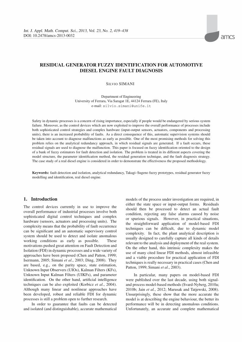
considered have barely detectable effects on anymeasurements, which represents the most challengingsituation. On the other hand, these faults can be diagnosedusing the strategy described in Sections 4 and 5. As anexample, Fig. 5 depicts the engine measured temperaturesignal affected by a fault commencing at 850 s, whose rateis fixed in order to produce an error of about 5% per houron the corresponding temperature measurement u4(k).

0 500 1000 1500 2000 2500 3000 350020

40

60

80

100

Time (s.)

y p

Fig. 5. Fault-free (continuous black) and faulty (dashed grey)engine temperature measurement x = u4(k).

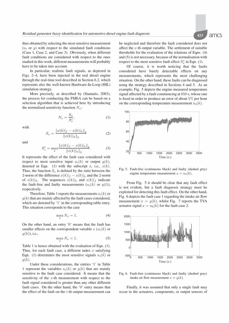
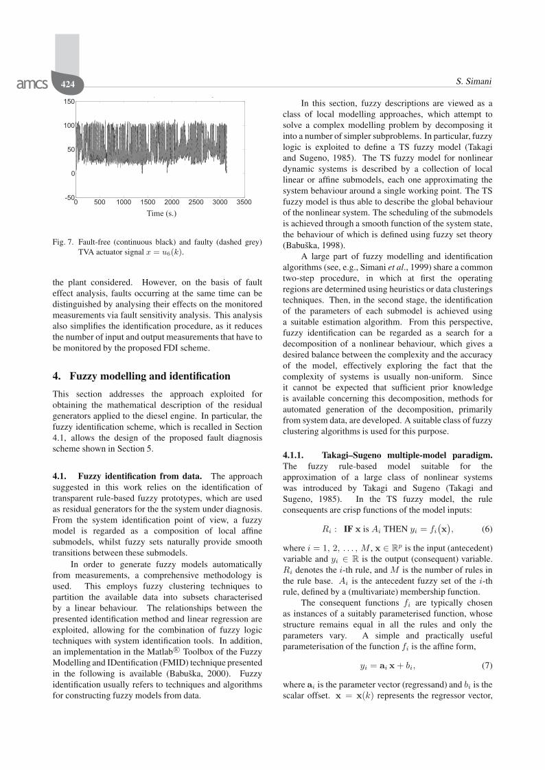
From Fig. 5 it should be clear that any fault effectis not evident, but a fault diagnosis strategy must beexploited for detecting this fault effect. On the other hand,Fig. 6 depicts the fault case 1 regarding the intake air flowmeasurement x = y(k), whilst Fig. 7 reports the TVAactuator signal x = u6(k) for the fault case 2.

Time (s.)

y

0 500 1000 1500 2000 2500 3000 3500-500

0

500

1000

1500

2000

Fig. 6. Fault-free (continuous black) and faulty (dashed grey)intake air flow measurement x = y(k).

Finally, it was assumed that only a single fault mayoccur in the actuators, components, or output sensors of

424 S. Simani

Time (s.)

y g

0 500 1000 1500 2000 2500 3000 3500-50

0

50

100

150

Fig. 7. Fault-free (continuous black) and faulty (dashed grey)TVA actuator signal x = u6(k).

the plant considered. However, on the basis of faulteffect analysis, faults occurring at the same time can bedistinguished by analysing their effects on the monitoredmeasurements via fault sensitivity analysis. This analysisalso simplifies the identification procedure, as it reducesthe number of input and output measurements that have tobe monitored by the proposed FDI scheme.

4. Fuzzy modelling and identification

This section addresses the approach exploited forobtaining the mathematical description of the residualgenerators applied to the diesel engine. In particular, thefuzzy identification scheme, which is recalled in Section4.1, allows the design of the proposed fault diagnosisscheme shown in Section 5.

4.1. Fuzzy identification from data. The approachsuggested in this work relies on the identification oftransparent rule-based fuzzy prototypes, which are usedas residual generators for the the system under diagnosis.From the system identification point of view, a fuzzymodel is regarded as a composition of local affinesubmodels, whilst fuzzy sets naturally provide smoothtransitions between these submodels.

In order to generate fuzzy models automaticallyfrom measurements, a comprehensive methodology isused. This employs fuzzy clustering techniques topartition the available data into subsets characterisedby a linear behaviour. The relationships between thepresented identification method and linear regression areexploited, allowing for the combination of fuzzy logictechniques with system identification tools. In addition,an implementation in the Matlab R© Toolbox of the FuzzyModelling and IDentification (FMID) technique presentedin the following is available (Babuska, 2000). Fuzzyidentification usually refers to techniques and algorithmsfor constructing fuzzy models from data.

In this section, fuzzy descriptions are viewed as aclass of local modelling approaches, which attempt tosolve a complex modelling problem by decomposing itinto a number of simpler subproblems. In particular, fuzzylogic is exploited to define a TS fuzzy model (Takagiand Sugeno, 1985). The TS fuzzy model for nonlineardynamic systems is described by a collection of locallinear or affine submodels, each one approximating thesystem behaviour around a single working point. The TSfuzzy model is thus able to describe the global behaviourof the nonlinear system. The scheduling of the submodelsis achieved through a smooth function of the system state,the behaviour of which is defined using fuzzy set theory(Babuska, 1998).

A large part of fuzzy modelling and identificationalgorithms (see, e.g., Simani et al., 1999) share a commontwo-step procedure, in which at first the operatingregions are determined using heuristics or data clusteringstechniques. Then, in the second stage, the identificationof the parameters of each submodel is achieved usinga suitable estimation algorithm. From this perspective,fuzzy identification can be regarded as a search for adecomposition of a nonlinear behaviour, which gives adesired balance between the complexity and the accuracyof the model, effectively exploring the fact that thecomplexity of systems is usually non-uniform. Sinceit cannot be expected that sufficient prior knowledgeis available concerning this decomposition, methods forautomated generation of the decomposition, primarilyfrom system data, are developed. A suitable class of fuzzyclustering algorithms is used for this purpose.

4.1.1. Takagi–Sugeno multiple-model paradigm.The fuzzy rule-based model suitable for theapproximation of a large class of nonlinear systemswas introduced by Takagi and Sugeno (Takagi andSugeno, 1985). In the TS fuzzy model, the ruleconsequents are crisp functions of the model inputs:

Ri : IF x is Ai THEN yi = fi

(x), (6)

where i = 1, 2, . . . , M , x ∈ Rp is the input (antecedent)

variable and yi ∈ R is the output (consequent) variable.Ri denotes the i-th rule, and M is the number of rules inthe rule base. Ai is the antecedent fuzzy set of the i-thrule, defined by a (multivariate) membership function.

The consequent functions fi are typically chosenas instances of a suitably parameterised function, whosestructure remains equal in all the rules and only theparameters vary. A simple and practically usefulparameterisation of the function fi is the affine form,

yi = ai x + bi, (7)

where ai is the parameter vector (regressand) and bi is thescalar offset. x = x(k) represents the regressor vector,


which can contain delayed samples of u(k) and y(k). Thismodel is referred to as the affine TS model, and can bewritten as (Takagi and Sugeno, 1985)

y =∑M

i=1 μi(x) yi∑M

i=1 μi(x). (8)

The antecedent fuzzy sets μi are extracted from thefuzzy partition matrix (Babuska, 1998). The consequentparameters ai and bi are estimated from the data usingthe method developed by the author (Simani et al., 1999)and recalled below. This identification scheme exploitedfor the estimation of TS model parameters has beenintegrated into the FMID toolbox for Matlab R© by theauthor. This approach developed by the author is usuallypreferred when the TS model should serve as a predictor,as it computes the consequent parameters via the Frischscheme, developed for errors-in-variables descriptions(Van Huffel and Lemmerling, 2002). Therefore, afterthe clustering of the data has been obtained via theGK algorithm (Babuska, 1998), the data subsets areprocessed according to the Frisch scheme identificationprocedure (Simani et al., 1999), in order to estimate theTS parameters for each affine submodel.

4.1.2. Fuzzy identification from clusters. As statedabove, the GK fuzzy clustering algorithm is used toapproximate a data set by local affine models. In orderto obtain a description useful for prediction purposes,an additional step must be applied to generate modelsindependent of the identification data. This section recallsthe algorithm for constructing fuzzy TS prototypes fromfuzzy partitions.

The antecedent fuzzy sets Ai can be computedanalytically in the antecedent product space or extractedfrom the fuzzy partition matrix. The consequentparameters ai and bi are estimated from the data usingthe method sketched in the following. The antecedentmembership functions can be obtained by projectingthe fuzzy partition onto the antecedent variables orcomputing the membership degrees directly in the productspace of the antecedent variables. These methods areavailable from the FMID toolbox for Matlab R© (Babuska,2000) developed by Robert Babuska (Babuska, 1998).The method exploited in this study is the second one,which considers multi-dimensional antecedent member-ship functions, represented analytically by computingan inverse of the distance from the cluster prototype.The membership degree is computed directly for theentire input vector (without the decomposition). Theantecedents of the TS rules are simple propositions withmulti-dimensional fuzzy sets μ(x) of Eqn. (8).

Regarding the estimation of the consequentparameters, they are derived using the procedure recalledin the following and developed by the author and

his co-workers (Simani et al., 1999). This approachis preferred when TS descriptions should serve aspredictors.

Thus, after the clustering of the data has beenobtained, in order to identify the structure of the TSprototype of Eqn. (8) in the i-th cluster, with i =1, . . . , K , and K clusters, the following matrices aredefined:

X(i)n =

⎡

⎢⎢⎢⎣

y(k) xTn (0) 1

y(k + 1) xTn (1) 1

......

...y(k + Ni − 1) xT

n (Ni − 1) 1

⎤

⎥⎥⎥⎦

, (9)

where the subscript n represents the order of the dynamicmodel considered (number of regressors), i.e., xn(h) =[y(h − 1), . . . , y(h − n), u(h − 1), . . . , u(h − n)]T .Therefore

Σ(i)n =

(X(i)

n

)T

X(i)n . (10)

In order to solve the so-called noise-rejection problem(Simani et al., 1999) in a mathematical framework, it isnecessary to follow the assumptions that the noises u(k)and y(k) are additive on the input-output data u∗(k) andy∗(k), and region independent (k = 1, 2, . . . , N ).

Under these assumptions, a positive-definite matrixΣ(i)

n associated to the sequences belonging to the i-thcluster can be expressed as the sum of two terms Σ(i)

n =Σ∗(i)

n + ¯Σn, where

¯Σn = diag[¯σyIn+1, ¯σuIn, 0] ≥ 0. (11)

The solution of the above identification problem requiresthe computation of the unknown noise covariances ¯σu and¯σy , which can be achieved by solving the relation

Σ∗(i)n = Σ(i)

n − Σn ≥ 0 (12)

in the variables σu, σy , where

Σn = diag[σyIn+1, σuIn, 0].

It is worth noting that all the surfaces defined by Eqn. (12)have necessarily at least one common point, i.e., the point(¯σu, ¯σy) corresponding to the true variances of the noiseaffecting the input and the output data.

The search for a solution to the identificationproblem can therefore start from the determination of thispoint in the noise space, if the noise characteristics arecommon to all the clusters and all assumptions regardingthe Frisch scheme are satisfied (independence betweeninput-output sequences, additive noise, noise whiteness)(Van Huffel and Lemmerling, 2002).

However, in real cases, these assumptions have tobe relaxed. Thus no common point can be determinedamong surfaces Γ(i)

n = 0 (i.e., the locus of the points

426 S. Simani

satisfying Eqn. (12) in the noise plane, and a uniquesolution to the identification problem cannot be obtained.In this situation, local fuzzy model identification can beperformed by finding a point (σu, σy) ∈ Γ(i)

n+1 = 0 that

makes Σ∗(i)n+1 closer to the double singular condition. It

leads to determining the common point of the surfaceseven when the assumptions of the Frisch scheme areslightly violated. Moreover, for each i-th cluster, differentnoises (¯σ(i)

u , ¯σ(i)y ) and the following relation should be

rewritten as

Σ∗(i)n = Σ(i)

n − Σ(i)n ≥ 0, (13)

where Σ(i)n = diag[¯σ(i)

u In+1, ¯σ(i)y In, 0] whilst (¯σ(i)

u , ¯σ(i)y )

represent the variances of input and output additive noisesin the i-th cluster. The identification scheme considerednormally assumes that (Van Huffel and Lemmerling,2002) {

u(k) = u∗(k) + u(k),y(k) = y∗(k) + y(k), (14)

where u∗(k) and y∗(k) are the noise-free data noise termsu(k) and y(k) are independent of every other term, andonly u(k) and y(k) are known.

Finally, the matrices Σ(i)n can therefore be built

and the parameter of the model in each cluster can bedetermined by means of the relation:

(Σ(i)n − Σ(i)

n )a(i) = 0, i = 1, . . . , K, (15)

for K clusters. This completes the fuzzy identificationprocedure in the fuzzy environment.

Finally, on the basis of the results achieved here,Section 5 will describe the design of residual generatorsin the form of fuzzy TS prototypes of Eqn. (8) for the FDIof the diesel engine considered.

5. Fault diagnosis scheme design

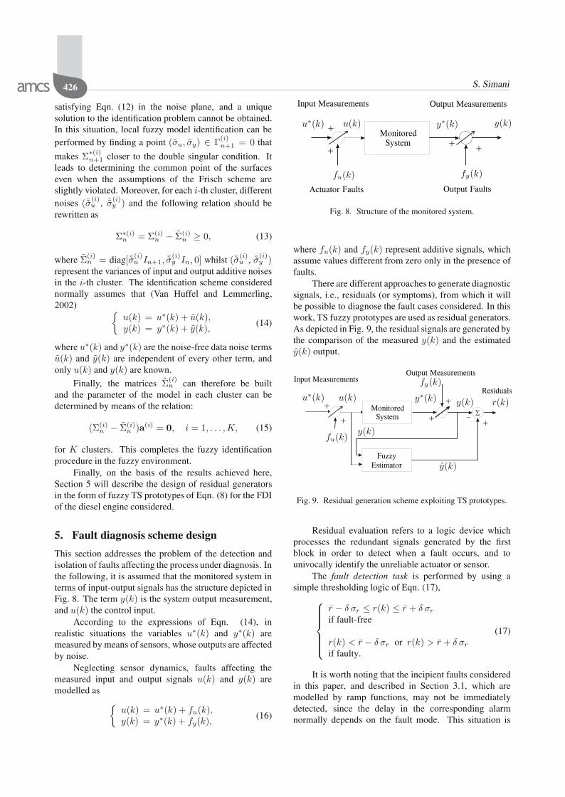
This section addresses the problem of the detection andisolation of faults affecting the process under diagnosis. Inthe following, it is assumed that the monitored system interms of input-output signals has the structure depicted inFig. 8. The term y(k) is the system output measurement,and u(k) the control input.

According to the expressions of Eqn. (14), inrealistic situations the variables u∗(k) and y∗(k) aremeasured by means of sensors, whose outputs are affectedby noise.

Neglecting sensor dynamics, faults affecting themeasured input and output signals u(k) and y(k) aremodelled as

{u(k) = u∗(k) + fu(k),y(k) = y∗(k) + fy(k), (16)

Output Measurements

++

+

+

MonitoredSystem

Input Measurements

Actuator Faults Output Faults

u∗(k) y∗(k) y(k)u(k)

fu(k) fy(k)

Fig. 8. Structure of the monitored system.

where fu(k) and fy(k) represent additive signals, whichassume values different from zero only in the presence offaults.

There are different approaches to generate diagnosticsignals, i.e., residuals (or symptoms), from which it willbe possible to diagnose the fault cases considered. In thiswork, TS fuzzy prototypes are used as residual generators.As depicted in Fig. 9, the residual signals are generated bythe comparison of the measured y(k) and the estimatedy(k) output.

+

+

+

_ �

Residuals

+

+

Fuzzy

Estimator

MonitoredSystem

Input MeasurementsOutput Measurements

u∗(k) y∗(k)

y(k)

y(k)u(k)

fu(k)

fy(k)

y(k)

r(k)

Fig. 9. Residual generation scheme exploiting TS prototypes.

Residual evaluation refers to a logic device whichprocesses the redundant signals generated by the firstblock in order to detect when a fault occurs, and tounivocally identify the unreliable actuator or sensor.

The fault detection task is performed by using asimple thresholding logic of Eqn. (17),

⎧⎪⎪⎪⎪⎨

⎪⎪⎪⎪⎩

r − δ σr ≤ r(k) ≤ r + δ σr

if fault-free

r(k) < r − δ σr or r(k) > r + δ σr

if faulty.

(17)

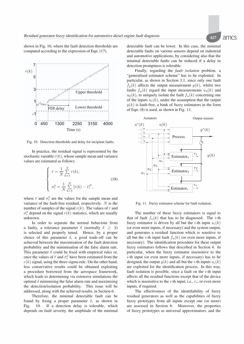
It is worth noting that the incipient faults consideredin this paper, and described in Section 3.1, which aremodelled by ramp functions, may not be immediatelydetected, since the delay in the corresponding alarmnormally depends on the fault mode. This situation is


shown in Fig. 10, where the fault detection thresholds arecomputed according to the expression of Eqn. (17).

-1

1

3

5

7

0 450 1300 2250 3150 4000

Time (s)

FDI delay

Upper threshold

Lower threshold

r(k)

Fig. 10. Detection thresholds and delay for incipient faults.

In practice, the residual signal is represented by thestochastic variable r(k), whose sample mean and variancevalues are estimated as follows:

⎧⎪⎪⎪⎪⎨

⎪⎪⎪⎪⎩

r =1N

N∑

k=1

r(k),

σ2r =

1N

N∑

k=1

[r(k) − r]2 ,

(18)

where r and σ2r are the values for the sample mean and

variance of the fault-free residual, respectively. N is thenumber of samples of the signal r(k). The values of r andσ2

r depend on the signal r(k) statistics, which are usuallyunknown.

In order to separate the normal behaviour froma faulty, a tolerance parameter δ (normally δ ≥ 2)is selected and properly tuned. Hence, by a properchoice of this parameter δ, a good trade-off can beachieved between the maximisation of the fault detectionprobability and the minimisation of the false alarm rate.This parameter δ could be fixed with empirical rules or,once the values of r and σ2

r have been estimated from ther(k) signal, using the three-sigma rule. On the other hand,less conservative results could be obtained exploitinga procedure borrowed from the aerospace framework,which leads to determining via extensive simulations theoptimal δ minimising the false alarm rate and maximisingthe detection/isolation probability. This issue will beaddressed, along with the achieved results, in Section 6.

Therefore, the minimal detectable fault can befound by fixing a proper parameter δ, as shown inFig. 10. If a detection delay is tolerable, whichdepends on fault severity, the amplitude of the minimal

detectable fault can be lower. In this case, the minimaldetectable faults on various sensors depend on industrialand automotive applications, by considering also that theminimal detectable faults can be reduced if a delay indetection promptness is tolerable.

Finally, regarding the fault isolation problem, a“generalised estimator scheme” has to be exploited. Inparticular, as shown in Section 3.1, since only one faultfy(k) affects the output measurement y(k), whilst twofaults fu(k) regard the input measurements u4(k) andu6(k), to uniquely isolate the fault fu(k) concerning oneof the inputs ui(k), under the assumption that the outputy(k) is fault-free, a bank of fuzzy estimators in the formof Eqn. (8) is used, as shown in Fig. 11.

...

..

.

.

... .

.

..

..

..

Actuators Output sensors

u(k)u∗(k)y∗(k)

y(k)

Process

r1

r2

rr

u1

u2

u3

ur

Estimator1

Estimator2

Estimatorr

Fig. 11. Fuzzy estimator scheme for fault isolation.

The number of these fuzzy estimators is equal tothat of fault fu(k) that has to be diagnosed. The i-thfuzzy estimator is driven by all but the i-th input ui(k)(or even more inputs, if necessary) and the system output,and generates a residual function which is sensitive toall but the i-th input fault fu(k) (or even more inputs, ifnecessary). The identification procedure for these outputfuzzy estimators follows that described in Section 4. Inparticular, when the fuzzy estimator insensitive to thei-th input (or even more inputs, if necessary) has to bedesigned, the output y(k) and all but the i-th inputs ui(k)are exploited for the identification process. In this way,fault isolation is possible, since a fault on the i-th inputaffects all the residual functions except that of the devicewhich is insensitive to the i-th input, i.e., ri, or even moreinputs, if required.

The effectiveness of the identifiability of fuzzyresidual generators as well as the capabilities of fuzzyfuzzy prototypes from all inputs except one (or more)are assessed in Section 6. Moreover, the propertiesof fuzzy prototypes as universal approximators, and the

428 S. Simani

identification capabilities of fuzzy output predictors havebeen investigated, e.g., by Simani et al. (2003), Rovatti(1996), or Fantuzzi and Rovatti (1996).

In order to summarise the isolation capabilities of thepresented schemes, Table 2 shows the so-called fault sig-nature for the case of a single fault in each input signal.

Table 2. Fault signatures.u1 u2 . . . ur

r1 0 1 . . . 1r2 1 0 . . . 1...

......

......

rr 1 1 . . . 0

The residuals which are affected by input faults aredescribed by an entry ‘1’ in the corresponding table entry,while an entry ‘0’ means that the fault considered doesnot affect the corresponding residual. Note that, withreference to the present study, it is not necessary to isolatefaults in the system output y(k) since it is assumed thatonly one single fault can occur on the process output,which is a scalar signal y(k).

This work does not consider the fault estimationproblem, which was addressed in other works by the sameauthor ((Bonfe et al., 2011) but using a different approach.However, fuzzy TS models, which are used here asresidual generators, could be exploited for fault signalreconstruction, as shown, e.g., by Xu et al. (2012), in thesame way as for neural networks (Korbicz et al., 2004).

Finally, it is worth noticing that the identified fuzzyprototypes for residual generation can be easily simulatedon-line, once the optimisation stages have been performedoff-line, since they are equivalent to look-up tables andthus easily implementable by standard ECUs.

6. Experimental results

This section describes experimentations with the methodproposed for the fuzzy identification technique orientedto the design of fuzzy residual generators used for dieselengine fault diagnosis.

6.1. Diesel engine modelling validation. The fuzzyidentification procedure recalled in Section 4 exploitsthe design of fault diagnosis residual generators basedon identified TS fuzzy prototypes. In particular, oncethe input-output data have been acquired from the realdiesel engine process, both residual generator parameteridentification and fuzzy clustering tasks have beenperformed off-line.

It is assumed that the monitored diesel engine,depicted in Fig. 1, normally works in nominalfault-free conditions. In general, the process operates in

different working conditions, and the seven input-outputmeasurements u(k) and y(k), including temperatures,flows, control signals, and speed, can be acquired witha sampling rate Ts = 0.1 s.

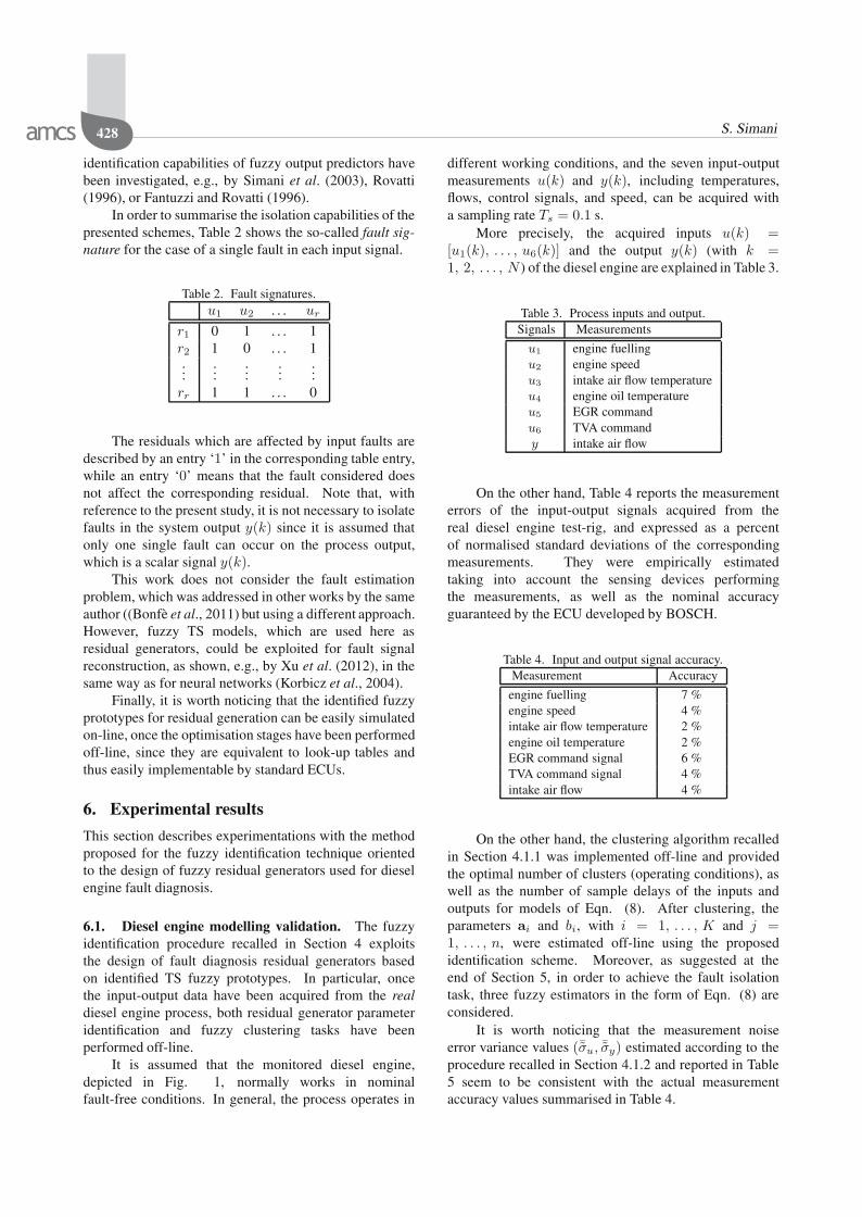
More precisely, the acquired inputs u(k) =[u1(k), . . . , u6(k)] and the output y(k) (with k =1, 2, . . . , N ) of the diesel engine are explained in Table 3.

Table 3. Process inputs and output.Signals Measurements

u1 engine fuellingu2 engine speedu3 intake air flow temperatureu4 engine oil temperatureu5 EGR commandu6 TVA commandy intake air flow

On the other hand, Table 4 reports the measurementerrors of the input-output signals acquired from thereal diesel engine test-rig, and expressed as a percentof normalised standard deviations of the correspondingmeasurements. They were empirically estimatedtaking into account the sensing devices performingthe measurements, as well as the nominal accuracyguaranteed by the ECU developed by BOSCH.

Table 4. Input and output signal accuracy.Measurement Accuracy

engine fuelling 7 %engine speed 4 %intake air flow temperature 2 %engine oil temperature 2 %EGR command signal 6 %TVA command signal 4 %intake air flow 4 %

On the other hand, the clustering algorithm recalledin Section 4.1.1 was implemented off-line and providedthe optimal number of clusters (operating conditions), aswell as the number of sample delays of the inputs andoutputs for models of Eqn. (8). After clustering, theparameters ai and bi, with i = 1, . . . , K and j =1, . . . , n, were estimated off-line using the proposedidentification scheme. Moreover, as suggested at theend of Section 5, in order to achieve the fault isolationtask, three fuzzy estimators in the form of Eqn. (8) areconsidered.

It is worth noticing that the measurement noiseerror variance values (¯σu, ¯σy) estimated according to theprocedure recalled in Section 4.1.2 and reported in Table5 seem to be consistent with the actual measurementaccuracy values summarised in Table 4.


Table 5. Estimated measurement noise variance values(¯σu, ¯σy).

Measurement Accuracy

engine fuelling 7.06 %engine speed 3.99 %intake air flow temperature 1.81 %engine oil temperature 1.93 %EGR command signal 5.78 %TVA command signal 3.82 %intake air flow 3.96 %

According to Figs. 9 and 11, the required faultdiagnosis residuals are generated by three TS fuzzyMultiple-Input Single-Output (MISO) prototypes ofEqn. (8). Thus, by following the scheme of Fig. 11,one fuzzy predictor used for the computation ofthe residual r1(k) is fed by the output y(k) andfour inputs [u1(k), u2(k), u3(k), u5(k)] with K =7 and n = 3. The second fuzzy estimatorgenerating r3(k) is fed by y(k) and five inputs, e.g.,[u1(k), u2(k), u3(k), u5(k), u6(k)] with K = 7 andn = 3. Finally, the third fuzzy estimator for r2(k)is fed by y(k) and [u1(k), u2(k), u3(k), u4(k), u5(k)]with K = 7 and n = 3. The membership degrees μi

required by the fuzzy estimators of Eqn. (8) have beenapproximated with Gaussian functions, whose parametershave been estimated by the fuzzy clustering algorithm(Babuska, 2000).

Therefore, the complete fuzzy estimator strategyis obtained by following Table 1, as these estimators,organised into a bank structure, after fault detectionallow performing also the required fault isolation task, asdescribed in Section 5.

It is worth noticing that the identified fuzzyprototypes for residual generation have been easilysimulated on-line, once the optimisation stages have beenperformed off-line. The computation time required forthe simulation of fuzzy TS models is quite low, thusallowing, if necessary, real-time generation of the residualsignals r(k). However, the computation time required forboth model estimation and optimisation is not crucial heresince these tasks are performed off-line at the FDI schemedesign stage.

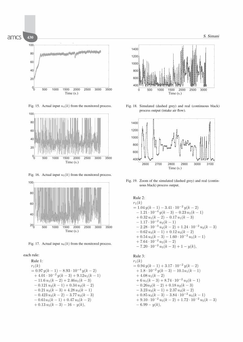
As an example, Figs. 12–17 depict one of the datasets containing the inputs signals u(k) generated from theprocess under diagnosis.

Note that the range limitations of the u5(k) andu6(k) signals depicted in Figs. 16 and 17 are due tothe control strategies implemented by the ECU BOSCHcontroller used by VM Motors S.p.A.

On the other hand, the actual output measurement,y(k), compared with the signal reconstructed by the fuzzyestimator, is reported in Fig. 18.

0 500 1000 1500 2000 2500 3000 35000

20

40

60

80

100

g g

Time (s.)

Fig. 12. Actual input u1(k) from the monitored process.

g p

Time (s.)

0 500 1000 1500 2000 2500 3000 35000

1000

2000

3000

4000


p

Time (s.)

0 500 1000 1500 2000 2500 3000 350020

40

60

80

100


In order to highlight the performance of TS fuzzymodels, Fig. 19 represent the zoom of the actualoutput measurement, y(k), compared with the signalreconstructed by the fuzzy estimator for r1(k) residualgeneration.

In the following, the structure of fuzzy residualgenerators is reported. In particular, regarding thegeneration of the residual r1(k) on the basis of the signalsu1(k), u2(k), u3(k), u5(k), and y(k), the identifiedconsequents are reported in the following expressions for

430 S. Simanig p

Time (s.)0 500 1000 1500 2000 2500 3000 3500

0

20

40

60

80

100


Time (s.)

0 500 1000 1500 2000 2500 3000 35000

20

40

60

80

100


Time (s.)0 500 1000 1500 2000 2500 3000 3500

20

40

60

80

100


each rule:

Rule 1:r1(k)= 0.97 y(k − 1) − 8.93 · 10−4 y(k − 2)

+ 4.01 · 10−2 y(k − 3) + 9.12u1(k − 1)− 11.6 u1(k − 2) + 2.46u1(k − 3)− 0.121 u2(k − 1) + 0.34 u2(k − 2)− 0.21 u2(k − 3) + 4.28 u3(k − 1)− 0.423 u3(k − 2) − 3.77 u3(k − 3)− 0.61u5(k − 1) + 0.47 u5(k − 2)+ 0.13 u5(k − 3) − 16 − y(k),

Time (s.)0 500 1000 1500 2000 2500 3000

400

600

800

1000

1200

1400

Fig. 18. Simulated (dashed grey) and real (continuous black)process output (intake air flow).

( )

Time (s.)2600 2700 2800 2900 3000 3100

400

600

800

1000

1200

1400

Fig. 19. Zoom of the simulated (dashed grey) and real (contin-uous black) process output.

Rule 2:r1(k)= 1.04 y(k − 1) − 3.41 · 10−2 y(k − 2)− 1.21 · 10−4 y(k − 3) − 0.23 u1(k − 1)+ 0.32 u1(k − 2) − 0.17 u1(k − 3)− 1.17 · 10−2 u2(k − 1)− 2.28 · 10−3 u2(k − 2) + 1.24 · 10−2 u2(k − 3)− 0.62 u3(k − 1) + 0.12 u3(k − 2)+ 0.54 u3(k − 3) − 1.60 · 10−2 u5(k − 1)+ 7.64 · 10−2 u5(k − 2)− 7.20 · 10−2 u5(k − 3) + 1 − y(k),

Rule 3:r1(k)= 0.94 y(k − 1) + 3.17 · 10−2 y(k − 2)

+ 1.8 · 10−2 y(k − 3) − 10.1u1(k − 1)+ 4.08 u1(k − 2)+ 6 u1(k − 3) + 8.74 · 10−2 u2(k − 1)− 0.26u2(k − 2) + 0.18 u2(k − 3)− 3.23 u3(k − 1) + 2.37 u3(k − 2)+ 0.85 u3(k − 3) − 3.84 · 10−2 u5(k − 1)+ 9.10 · 10−2 u5(k − 2) + 1.72 · 10−2 u5(k − 3)− 6.99 − y(k),


Rule 4:r1(k)= 0.97 y(k − 1) + 3.01 · 10−2 y(k − 2)

+ 1.14 · 10−2 y(k − 3) + 2.97 u1(k − 1)− 5.10 u1(k − 2) + 1.99 u1(k − 3)+ 1.38 · 10−2 u2(k − 1)− 1.56 · 10−2 u2(k − 2) − 2.12 · 10−3 u2(k − 3)+ 1.75 u3(k − 1) + 0.35 u3(k − 2)− 2.03 u3(k − 3) − 0.27 u5(k − 1)− 0.34u5(k − 2)+ 0.62 u5(k − 3) − 1.23 − y(k),

Rule 5:r1(k)= 0.92 y(k − 1) + 7.75 · 10−2 y(k − 2)

+ 5.99 · 10−3 y(k − 3) + 6.54 u1(k − 1)− 2.84 u2(k − 2) − 3.82 u1(k − 3)− 4.95 · 10−2 u2(k − 1)+ 6.97 · 10−2 u2(k − 2) − 2.66 · 10−2 u2(k − 3)+ 4.44 u3(k − 1) − 0.89 u3(k − 2)− 3.28 u3(k − 3) + 0.41 u5(k − 1) − 1.15 u5(k − 2)+ 0.75 u5(k − 3) − 1.65 − y(k),

Rule 6:r1(k)= 0.93 y(k − 1) + 4.43 · 10−2 y(k − 2)

+ 1.46 · 10−2 y(k − 3) + 1.87 · 10−2 u1(k − 1)+ 9.39 · 10−2 u1(k − 2) − 7.07 · 10−2 u1(k − 3)+ 6.48 · 10−2 u2(k − 1) − 7.11 · 10−2, u2(k − 2)+ 1.09 · 10−2 u2(k − 3) + 2.62 u3(k − 1)− 1.61 u3(k − 2) − 0.92 u3(k − 3)+ 0.18 u5(k − 1) − 0.65 u5(k − 2)+ 0.51 u5(k − 3) − 12.4 − y(k),

Rule 7:r1(k)= 1.07 y(k − 1) − 9.76 · 10−2 y(k − 2)

+ 2.79 · 10−2 y(k − 3) − 0.38 u1(k − 1)+ 0.46 u1(k − 2) − 0.14 u1(k − 3)+ 3.27 · 10−3 u2(k − 1)+ 9.10 · 10−2 u2(k − 2)− 9.84 · 10−2 u2(k − 3)− 1.31 u3(k − 1) + 1.23 u3(k − 2)+ 0.25 u3(k − 3) − 3.29 u5(k − 1)+ 2.16 u5(k − 2) + 1.15 u5(k − 3)− 2.38 − y(k).

(19)On the other hand, the structure of the fuzzy TS

prototype for the generation of the residual r2(k), whichdepends on y(k), u1(k), u2(k), u3(k), u4(k), and u5(k),is reported in the following expressions for each rule, withK = 7 and n = 3:

Rule 1:r2(k)= 1.01 y(k − 1) + 6.55 · 10−2y(k − 2)

− 7.19 · 10−2y(k − 3) − 5.06 u1(k − 1)+ 3.01 u1(k − 2) + 2.03 u1(k − 3)+ 0.21 u2(k − 1) − 0.17 u2(k − 2)+ 1.67 · 10−2 u2(k − 3) − 2.16 u3(k − 1)+ 0.19 u3(k − 2) + 1.95 u3(k − 3)+ 0.93 u4(k − 1) + 1.84 u4(k − 2)− 2.86 u4(k − 3) + 5.29 · 10−2 u5(k − 1)0.39 u5(k − 2) − 0.5 u5(k − 3) − 139 − y(k),

Rule 2:r2(k)= 1.07 y(k − 1) − 1.79 · 10−2 y(k − 2)− 5.11 · 10−2 y(k − 3) − 0.14 u1(k − 1)− 0.74 u1(k − 2) + 0.89 u1(k − 3)+ 4.07 · 10−3 u2(k − 1)+ 3.68 · 10−3 u2(k − 2) − 1.07 · 10−2 u2(k − 3)+ 0.49 u3(k − 1) + 0.74 u3(k − 2)− 1.22 u3(k − 3) + 0.94 u4(k − 1)− 1.13 u4(k − 2) + 9.46 · 10−2 u4(k − 3)− 0.96 · u5(k − 1) + 1.02 u5(k − 2)− 7.86 · 10−2 u5(k − 3) + 11.2 − y(k),

Rule 3:r2(k)= 0.87 y(k − 1) + 4.42 · 10−2 y(k − 2)

+ 8.66 · 10−2 y(k − 3) + 0.84 u1(k − 1)+ 7.18 · 10−1 u1(k − 2) − 1.81 u1(k − 3)− 8.45 · 10−2 u2(k − 1) − 1.16 · 10−2 u2(k − 2)+ 9.07 · 10−2 u2(k − 3) + 1.35 u3(k − 1)− 0.59 u3(k − 2) − 0.45 u3(k − 3) − 1.88 u4(k − 1)+ 1.29 u4(k − 2) + 0.7 u4(k − 3) + 0.68 u5(k − 1)− 1.47 u5(k − 2) + 0.88 u5(k − 3) − 9.04 − y(k),

Rule 4:r2(k)= 0.95 y(k − 1) − 5.55 · 10−2 y(k − 2)

+ 7.72 · 10−2 y(k − 3)+ 1.67 u1(k − 1) − 0.71 u1(k − 2)− 0.89 u1(k − 3) + 3.24 · 10−2 u2(k − 1)− 3.62 · 10−2 u2(k − 2) − 7.09 · 10−4 u2(k − 3)− 2.16 u3(k − 1) − 2.40 u3(k − 2) + 4.35 u3(k − 3)+ 0.46 u4(k − 1) − 1.42 u4(k − 2) + 1.12 u4(k − 3)+ 2.14 u5(k − 1) − 0.88 u5(k − 2) − 1.18 u5(k − 3)+ 25.5 − y(k),

Rule 5:r2(k)= 0.8 y(k − 1) + 0.16 y(k − 2)

+ 8.05 · 10−2 y(k − 3) + 6.32 u1(k − 1)− 31 u1(k − 2) + 24.4 u1(k − 3)+ 1.72 · 10−2 u2(k − 1) + 0.14 u2(k − 2)− 0.14 u2(k − 3) + 12.2 u3(k − 1)+ 3.87 u3(k − 2) − 15.3 u3(k − 3)− 1.22 u4(k − 1) + 2.74 u4(k − 2) − 2.26 u4(k − 3)− 2.87 u5(k − 1) − 0.4 u5(k − 2) + 3.23 u5(k − 3)− 46.4 − y(k),

432 S. Simani

Rule 6:r2(k)= y(k − 1) − 1.80 · 10−2 y(k − 2)

+ 1.51 · 10−2 y(k − 3) + 0.18 u1(k − 1)+ 5.57 · 10−2 u1(k − 2) − 0.25 u1(k − 3)+ 8.68 · 10−3 u2(k − 1) + 4.53 · 10−3 u2(k − 2)+ 4.99 · 10−3 u2(k − 3) + 6.74 · 10−2 u3(k − 1)− 2.77 · 10−2 u3(k − 2) − 2.78 · 10−2 u3(k − 3)− 2.55 · 10−3 u4(k − 1) − 7.63 · 10−2 u4(k − 2)− 2.67 · 10−2 u4(k − 3) − 0.51 u5(k − 1)+ 0.19 u5(k − 2) + 0.31 u5(k − 3) + 6.53 − y(k),

Rule 7:r2(k)= 0.93 y(k − 1) − 5.66 · 10−2 y(k − 2)

+ 0.14 y(k − 3) + 2.87 u1(k − 1) + 0.33 u1(k − 2)− 3.5 u1(k − 3) − 0.19 u2(k − 1) + 0.27 u2(k − 2)− 0.13 u2(k − 3) + 3.28 u3(k − 1) − 0.45 u3(k − 2)− 2.14 u3(k − 3) − 1.48 u4(k − 1) − 2.17 u4(k − 2)+ 4.81 u4(k − 3) − 4.37 u5(k − 1) − 0.13 u5(k − 2)+ 4.64 u5(k − 3) − 22.9 − y(k).

(20)Finally, the structure of the fuzzy TS prototype for

the generation of the residual r3(k), which uses the signalsy(k), u1(k), u2(k), u3(k), u5(k), and u6(k), is reportedin the expressions for each rule, with K = 7 and n = 3:

Rule 1:r3(k)= 0.94 y(k − 1)

+ 6.36 · 10−2 y(k − 2) + 6.19 · 10−3 y(k − 3)+ 6.18 u1(k − 1) − 5.44 u1(k − 2)− 0.89 u1(k − 3) + 3.32 · 10−2 u2(k − 1)− 8.79 · 10−2 u2(k − 2) + 5.08 · 10−2 u2(k − 3)+ 2.67 u3(k − 1) − 0.24 u3(k − 2)− 2.28 u3(k − 3) + 0.48 u5(k − 1)− 1.26 u5(k − 2) + 0.79 u5(k − 3)− 0.35 u6(k − 1) + 1.27 u6(k − 2)− 0.93 u6(k − 3) − 1.98 − y(k),

Rule 2:r3(k)= 0.88 y(k − 1) + 0.16 y(k − 2)− 4.36 · 10−2 y(k − 3) + 1.13 u1(k − 1)− 2.21 u1(k − 2) + 1.11 u1(k − 3)− 1.81 · 10−2 u2(k − 1) − 0.28 u2(k − 2)+ 0.32 u2(k − 3) + 1.91 u3(k − 1)− 2.34 u3(k − 2) + 0.63 u3(k − 3)+ 1.87 u5(k − 1) − 1.51 u5(k − 2)− 0.34 u5(k − 3) + 0.35 u6(k − 1)− 0.48 u6(k − 2) + 0.13 u6(k − 3)− 70.9 − y(k),

Rule 3:r3(k)= 0.96 y(k − 1)

− 2.40 · 10−2 y(k − 2) + 6.28 · 10−2 y(k − 3)+ 0.77 u1(k − 1) − 8.32 u1(k − 2)+ 7.5 u1(k − 3) − 8.94 · 10−2 u2(k − 1)+ 0.18 u2(k − 2) − 9.69 · 10−2 u2(k − 3)+ 7.22 u3(k − 1) − 2.35 u3(k − 2)− 4.51 u3(k − 3) − 1.17 u5(k − 1)+ 0.35 u5(k − 2) + 0.85 u5(k − 3)+ 0.46 u6(k − 1) + 2.17 u6(k − 2)− 2.56 u6(k − 3) − 5.17 − y(k),

Rule 4:r3(k)= y(k − 1) − 4.86 · 10−2 y(k − 2)

4.44 · 10−2 y(k − 3) − 1.7 u1(k − 1)+ 3.31 u1(k − 2) − 1.51 u1(k − 3)− 9.95 · 10−3 u2(k − 1) + 0.25 u2(k − 2)− 0.25 u2(k − 3) − 0.95 u3(k − 1)+ 1.87 u3(k − 2) − 0.97 u3(k − 3)− 0.67 u5(k − 1) + 0.25 u5(k − 2)+ 0.38 u5(k − 3) − 0.53 u6(k − 1)+ 1.02 u6(k − 2) − 0.48 u6(k − 3) + 11.1 − y(k),

Rule 5:r3(k)= 0.99 y(k − 1)

+ 2.93 · 10−3 y(k − 2) + 6.6 · 10−3 y(k − 3)+ 3.06 u1(k − 1) − 3.11 u1(k − 2)+ 7.23 · 10−2 u1(k − 3) + 9.51 · 10−3 u2(k − 1)− 9.02 · 10−3 u2(k − 2) − 2.82 · 10−3 u2(k − 3)− 0.71 u3(k − 1) + 0.4 u3(k − 2)+ 0.41 u3(k − 3) − 0.98 u5(k − 1)+ 0.26 u5(k − 2) + 0.76 u5(k − 3)+ 0.23 u6(k − 1) − 0.21 u6(k − 2)− 5.73 · 10−3 u6(k − 3) − 2.06 − y(k),

Rule 6:r3(k)= 0.97 y(k − 1)− 2.10 · 10−2 y(k − 2) + 3.56 · 10−2 y(k − 3)− 25.1 u1(k − 1) + 24 u1(k − 2)+ 1.22 u1(k − 3) + 7.21 · 10−2 u2(k − 1)+ 6.72 · 10−2 u2(k − 2) − 0.14 u2(k − 3)− 7.18 u3(k − 1) + 9.71 u3(k − 2)− 2.49 u3(k − 3) − 2.25 u5(k − 1)+ 2.36 u5(k − 2) − 5.16 · 10−2 u5(k − 3)+ 0.11 u6(k − 1) − 1.86 u6(k − 2)+ 1.37 u6(k − 3) + 36.6 − y(k),

Rule 7:r3(k)= 1.18 y(k − 1)− 0.19 y(k − 2) + 2.16 · 10−2 y(k − 3)+ 0.41 u1(k − 1) − 0.75 u1(k − 2)+ 0.27 u1(k − 3) + 2.9 · 10−2 u2(k − 1)+ 5.69 · 10−4 u2(k − 2) − 3.61 · 10−2u2(k − 3)− 0.27 u3(k − 1) − 0.23 u3(k − 2)


+ 0.85 u3(k − 3) − 4.5 u5(k − 1) + 4.43 u5(k − 2)+ 0.13 u5(k − 3) + 0.32 u6(k − 1)− 0.85 u6(k − 2) + 0.53u6(k − 3) − 13 − y(k).

(21)The FDI scheme capabilities were then validated

by testing it on various real data sets, acquired froma Jeep Wrangler under an emission test, according theEuropean Union Driving Cycle (EUDC). It is assumed,in general, that faulty data can be “logically” separablefrom fault-free sequences generated by the process underdiagnosis.

By considering different test data sequences, Table 6reports the Predicted Per Cent Reconstruction Error(PPCRE), where the reconstruction error ri(k) infault-free conditions is computed as the differencebetween the actual diesel engine output y(k) and theoutput from the i-th residual generator. Since this error isnormalised with respect to the output standard deviation,it can be seen as the percentage of data that are notcorrectly explained by the identified TS models. Theresults summarised in Table 6 indicate that the fuzzyprototypes are able to generate reliable residual signals forreal diesel engine fault diagnosis.

Table 6. TS fuzzy model errors for different data sets.Data set PPCRE

r1(k) r2(k) r3(k)

estimation data 0.90% 0.87% 0.92%validation data 2.80% 1.80% 2.10%test data 4.20% 3.50% 4.00%

Using these identified TS fuzzy prototypes, thediesel engine FDI scheme design has been applied to theactual process, as shown in Section 6.2, whilst furtherexperiments are summarised in Section 6.3.

6.2. Real-time diagnostic implementation. Clearly,the presented fuzzy identification would require aconsiderable calculation effort if it were implementedon-line. State-of-the-art Engine Control Units (ECUs)would not be able to perform these algorithms inan appropriate time. Assuming that the growth incalculation power has been proceeding at high speed ofthe last few years, future ECUs should make sufficientcalculation time available within some years, where verysimple adaptation or identification algorithms could beimplemented. However, it is worth noticing that thecomplete fuzzy modelling oriented to the design ofthe FDI strategy suggested in this work was computedoff-line.

On the other hand, special real-time computersystems based on digital signal processors already allowimplementation and testing of the model-based designs

in vehicles or an engine test stand. In order to operatethe designed fuzzy predictors for an FDI purpose underrealistic fault and working conditions, a real-time systemwas implemented at a dynamic engine test stand whereit could be run parallel to the production car’s ECU.This system uses the production car sensors, and theinput-output messages of the ECU.

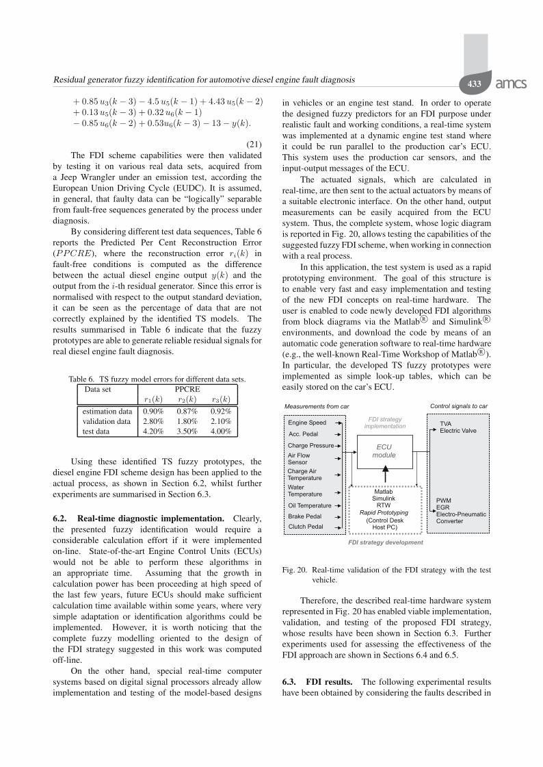
The actuated signals, which are calculated inreal-time, are then sent to the actual actuators by means ofa suitable electronic interface. On the other hand, outputmeasurements can be easily acquired from the ECUsystem. Thus, the complete system, whose logic diagramis reported in Fig. 20, allows testing the capabilities of thesuggested fuzzy FDI scheme, when working in connectionwith a real process.

In this application, the test system is used as a rapidprototyping environment. The goal of this structure isto enable very fast and easy implementation and testingof the new FDI concepts on real-time hardware. Theuser is enabled to code newly developed FDI algorithmsfrom block diagrams via the Matlab R© and Simulink R©environments, and download the code by means of anautomatic code generation software to real-time hardware(e.g., the well-known Real-Time Workshop of Matlab R©).In particular, the developed TS fuzzy prototypes wereimplemented as simple look-up tables, which can beeasily stored on the car’s ECU.

Engine Speed

Acc. Pedal

Charge Pressure

Air Flow

Sensor

Charge Air

Temperature

Water

Temperature

Oil Temperature

Brake Pedal

Clutch Pedal

Matlab

Simulink

RTW

Rapid Prototyping

TVA

Electric Valve

PWM

EGR

Electro-Pneumatic

Converter

ECU

module

(Control Desk

Host PC)

FDI strategy development

FDI strategy

implementation

Measurements from car Control signals to car

Fig. 20. Real-time validation of the FDI strategy with the testvehicle.

Therefore, the described real-time hardware systemrepresented in Fig. 20 has enabled viable implementation,validation, and testing of the proposed FDI strategy,whose results have been shown in Section 6.3. Furtherexperiments used for assessing the effectiveness of theFDI approach are shown in Sections 6.4 and 6.5.

6.3. FDI results. The following experimental resultshave been obtained by considering the faults described in

434 S. Simani

Section 3.1, and implemented in real-time, as describedin Section 6.2. They cause alteration of the signals ui(k)and y(k), and therefore of the residuals ri(k) given bythe predictive models in the form of Eqn. (8). Residualsindicate fault occurrence according to the logic of Eqn.(17), whether their values are lower or higher than thethresholds fixed in fault-free conditions.

As an example, Figs. 21, 23 and 25 show the resultsfrom the application of the fuzzy prototypes for residualgeneration.

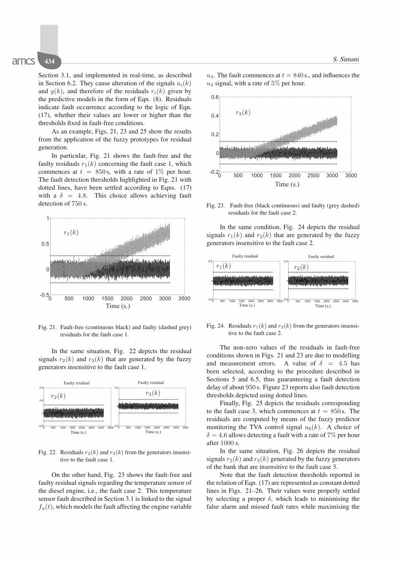
In particular, Fig. 21 shows the fault-free and thefaulty residuals r1(k) concerning the fault case 1, whichcommences at t = 850 s, with a rate of 1% per hour.The fault detection thresholds highlighted in Fig. 21 withdotted lines, have been settled according to Eqns. (17)with a δ = 4.8. This choice allows achieving faultdetection of 750 s.

Time (s.)

0 500 1000 1500 2000 2500 3000 3500-0.5

0

0.5

1

r1(k)

Fig. 21. Fault-free (continuous black) and faulty (dashed grey)residuals for the fault case 1.

In the same situation, Fig. 22 depicts the residualsignals r2(k) and r3(k) that are generated by the fuzzygenerators insensitive to the fault case 1.

Time (s.)

0 500 1000 1500 2000 2500 3000 3500-0.6

0

0.6

0.9

0 500 1000 1500 2000 2500 3000 3500-0.2

0

0.2

Time (s.)

Faulty residual Faulty residual

r2(k) r3(k)

Fig. 22. Residuals r2(k) and r3(k) from the generators insensi-tive to the fault case 1.

On the other hand, Fig. 23 shows the fault-free andfaulty residual signals regarding the temperature sensor ofthe diesel engine, i.e., the fault case 2. This temperaturesensor fault described in Section 3.1 is linked to the signalfu(t), which models the fault affecting the engine variable

u4. The fault commences at t = 840 s., and influences theu4 signal, with a rate of 5% per hour.

0 500 1000 1500 2000 2500 3000 3500-0.2

0

0.2

0.4

0.6

Time (s.)

r3(k)

Fig. 23. Fault-free (black continuous) and faulty (grey dashed)residuals for the fault case 2.

In the same condition, Fig. 24 depicts the residualsignals r1(k) and r2(k) that are generated by the fuzzygenerators insensitive to the fault case 2.

Time (s.)

0 500 1000 1500 2000 2500 3000 3500-0.6

0

0.6

Time (s.)

Faulty residualFaulty residual

0 500 1000 1500 2000 2500 3000 3500-0.5

0

0.5

r1(k) r2(k)


The non-zero values of the residuals in fault-freeconditions shown in Figs. 21 and 23 are due to modellingand measurement errors. A value of δ = 4.5 hasbeen selected, according to the procedure described inSections 5 and 6.5, thus guaranteeing a fault detectiondelay of about 950 s. Figure 23 reports also fault detectionthresholds depicted using dotted lines.

Finally, Fig. 25 depicts the residuals correspondingto the fault case 3, which commences at t = 850 s. Theresiduals are computed by means of the fuzzy predictormonitoring the TVA control signal u6(k). A choice ofδ = 4.6 allows detecting a fault with a rate of 7% per hourafter 1000 s.

In the same situation, Fig. 26 depicts the residualsignals r2(k) and r3(k) generated by the fuzzy generatorsof the bank that are insensitive to the fault case 3.

Note that the fault detection thresholds reported inthe relation of Eqn. (17) are represented as constant dottedlines in Figs. 21–26. Their values were properly settledby selecting a proper δ, which leads to minimising thefalse alarm and missed fault rates while maximising the


Time (s.)

0 500 1000 1500 2000 2500 3000 3500-0.5

0

0.5

1

r2(k)

Fig. 25. Fault-free (continuous black) and faulty (dashed grey)residuals for the fault case 3.

Time (s.)3500 0 500 1000 1500 2000 2500 3000 3500

-0.2

0

0.2

Time (s.)

Faulty residual Faulty residual

0 500 1000 1500 2000 2500 3000 3500-0.5

0

0.5 r1(k) r3(k)


correct detection and isolation rates. The optimisationprocedure for the selection of the parameter δ is furtherdiscussed in Section 6.5. These parameters depend on theautomotive application considered. In these conditions,the fault is correctly detected when the correspondingresidual signals exceed the thresholds by a fixed numberof consecutive samples.

Finally, it is worth observing that the developedstrategy based on fuzzy prototypes allows detecting andisolating realistic faults using uncertain measurementsacquired from the real diesel engine test-rig. Moreover,the real-time hardware system described in Section 6.2enabled the implementation, validation, and assessmentof the proposed FDI strategy, thus proving its reliabilityand robustness when applied also to real data. However,further investigations are shown in Sections 6.4 and 6.5.

6.4. Comparative studies. This section provides somecomparative results with respect to another FDI scheme,in particular, the one relying on a bank of UnknownInput Kalman Filters (UIKFs) (Chen and Patton, 1999).The UIKF bank was designed on the basis of a linearstate-space 15-th order model of the diesel engine, derivedon the basis of the identification method presented, e.g.,by Simani et al. (2000) and Simani (2007), but withoutexploiting the fuzzy multiple-model identification.

It is worth noticing that the state-space linearmodel of 15-th order was computed using a black-boxidentification procedure exploiting the subspace N4SIDalgorithm (Ljung, 1999). It is clear that, with referenceto this identified black-box state-space model, the statevariables do not have any physical meaning. In fact, themodel order was selected for achieving good estimationproperties. Moreover, this model was not derived fromany linearisation procedure, which motivates again thelack of any physical meaning of the state vector. Themodel structure was validated using the tools availablefrom the System Identification Toolbox (Ljung, 1997)developed in the Matlab R© environment. The validationis based on the auto- and cross-correlation analysis ofthe model estimation error, as described again by Ljung(1999). The suggested comparison between the UIKFapproach and fuzzy residual generators seems appropriateindeed. In fact, even if UIKFs are designed on the basis ofthe linear state-space model, they allow decoupling boththe model-reality mismatch and the measurement errors.In this way, UIKFs organised into a bank scheme forresidual generation are compared with TS fuzzy models.

Once the linear state-space 15-th order model forthe diesel engine has been computed, the UIKFs ofthe bank have been obtained by the design techniquedescribed, e.g., by Chen and Patton (1999, Section 3.5.1,pp. 99–108), while the noise covariance matrices havebeen estimated as described by Simani et al. (2001,Chapter 4, pp. 117–131). In particular, the design ofthe UIKFs of the bank is enhanced by the estimation ofthe noise covariance constant matrices directly achievedfrom the Frisch scheme, already exploited here, andrecalled in Section 4.1.2. Using the notation of Chenand Patton (1999, Section 3.5.1, p. 100), with theknowledge of the (constant) noise covariance matricesQk and Rk, which are computed from the identified(¯σu, ¯σy) (Simani, 2007), the time-varying gain Kk anderror covariance Pk matrices of the Kalman filter bank arecomputed. Therefore, the motivation for using the bank ofnon-stationary Kalman filter with unknown inputs here istwofold. First, the time-varying (non-stationary) Kalmanfilters designed on the basis of the linear state-space modelof the diesel engine are able to generate suitable residualsfor the nonlinear system. In practice, in this situation theidentified variance noise values (¯σu, ¯σy) take into accountthe uncertainty due to both modelling and measurementerrors, i.e., the disturbance term of the UIKFs (Simaniet al., 1999; Fantuzzi et al., 2002). Secondly, the bankof UIKFs allows us to achieve also the required faultisolation task, in the same way exploited for the designof the bank of fuzzy estimators, as described in Section 5.

As an example, the FDI residuals generated via theUIKF bank are shown in Fig. 27. In particular, the UIKFbank residuals relative to 2150 s. simulation time aredepicted in Fig. 27, when the fault cases 1, 2, and 3

436 S. Simani

commence at 850 s.

Time (s.)

0 500 1000 1500 2000 2500 3000 3500-0.4

-0.2

0

0.2

0.4

r1(k)

(a)

Time (s.)0 500 1000 1500 2000 2500 3000 3500

-0.2

-0.1

0

0.1

0.2

r3(k)

(b)

Time (s.)

0 500 1000 1500 2000 2500 3000 3500-0.4

-0.2

0

0.2

0.4

r2(k)

(c)

Fig. 27. UIKF fault-free (continuous black) and faulty (dashedgrey) residuals: case 1 fault residuals (a), case 2 faultresiduals (b), case 3 fault residuals (c).

The residual signals of Fig. 27 are different fromthose shown in the previous section. In this case in fact,the residual signals generated via the UIKF bank do notallow achieving the detection of the fault cases 1 and 3.Moreover, the detection of the fault case 2 is achievableonly if its rate is increased. Table 7 summarises the resultsobtained by comparing the FDI technique recalled in thissubsection.

A few comments can be drawn here. Whenthe modelling of the dynamic system can be perfectlyobtained, model-based schemes are preferred. In somesituations, the UIKF can take advantage of its noiseand disturbance rejection capabilities, but with quite

Table 7. Minimal detectable faults.Fault case UIKF Fuzzy approach

Case 1 Not detectable 1%

Case 2 15% 5%

Case 3 Not detectable 7%

complicated and not straightforward design procedures.However, in this case, the fault sensitivity of the linearUIKF is lower with respect to nonlinear fuzzy predictors.On the other hand, regarding the developed FDI fuzzymethod, it seems rather simple when developed inconnection with fuzzy identification, even if optimisationstages are required, for example, for optimal FDIthreshold selection. This further issue has been describedin Section 6.5

6.5. FDI scheme robustness evaluation. In thissection, further experimental results have been reportedregarding the performance optimisation and evaluationof the developed FDI scheme with respect to modellingerrors and measurement uncertainty. In particular, thesimulation of different fault-free and faulty data sequenceshas been performed by exploiting the test-rig setup ofSection 6.2 and a Matlab R© Monte-Carlo analysis. Infact, the Monte-Carlo tool is useful at this stage as FDIperformances depend the residual error magnitude as wellas on the measured signal u(k) and y(k) errors. Asremarked in Section 6.2, the experimental test-rig is ableto generate the required real-time signals and the injectionof realistic fault cases.

Moreover, as described in Section 5, it is assumedthat the input-output data u(k) and y(k) were affected bymeasurement errors. Thus, for performance evaluationand reliability analysis of the FDI scheme, some indiceshave been used. The performances of the FDI methodare thus empirically evaluated on 500 Monte-Carlo runs,corresponding to the same number of driving cycle tests.These indices are defined as follows:

False Alarm Rate (rfa): the number of wronglydetected faults divided by total fault cases;

Missed Fault Rate (rmf ): for each fault, the totalnumber of undetected faults, divided by the totalnumber of times that the fault case occurs;

True Detection/Isolation Rate (rtd, rti): for a particularfault case, the number of times it is correctlydetected/isolated, divided by total number of timesthat the fault case occurs;

Mean Detection/Isolation Delay (τmd, τmi): for aparticular fault case, the average detection/isolationdelay time.


These criteria are computed off-line for each fault case.Table 8 summarises the results obtained by consideringthe fuzzy residual generators, and with a choice of thethreshold parameter δ in Eqns. (17) leading to achieveoptimal results.

Table 8. Monte-Carlo analysis by monitoring residuals viaEqns. (17) with optimal δ.

Fault rfa rmf rtd, rti τmd, τmi δ

Case 1 0.002 0.003 0.997 750s 4.8

Case 2 0.001 0.001 0.999 950s 4.5

Case 3 0.002 0.003 0.997 1000s 4.6

Table 8 shows that with the proper selection of thethreshold levels depending on δ it is possible to achievefalse alarm and missed fault rates of less than 0.3%and detection and isolation rates larger than 99.7%, withminimal detection and isolation delay times. The resultsdemonstrate also that Monte-Carlo analysis is an effectivetool for experimentally testing the design robustness ofthe proposed FDI method with respect to error anduncertainty. This last simulation technique example hencefacilitates an assessment of the reliability of the developedFDI method applied to real test cases.

7. Conclusion

The paper provided practical results in the diagnosisof faults on a real diesel engine process by using amodel-based approach. The reported results show thatfaults having barely detectable effects on measurements,can be detected using residual generators in the form ofdynamic fuzzy Takagi–Sugeno prototypes. The outlinedmethod focused to some extent on identified input-outputmodels, thus the final fault diagnosis algorithm is basedonly on input-output processing of all measurable signals.

The paper suggested to exploit identifiedpiecewise-affine models, although the system consideredis strongly nonlinear. This is regarded as importantto avoid the complexities otherwise inevitable whenpurely nonlinear models are used. The algorithmicsimplicity can be seen as a very important aspect whenconsidering the need for verification and validation of ademonstrable scheme for industrial certification, mainlyimportant in automotive fields. This aspect of the work,together with the fact that the modelling uncertaintyand the measurement noise seem to be well tackled,confirms the straightforward application of the proposedfault diagnosis schemes to real automotive applications.Finally, the robustness and reliability properties wereinvestigated via extensive Monte–Carlo experiments.

Acknowledgment

The author would like to express his gratitude to VMMotors S.p.A. (Cento, Ferrara, Italy) for the financialsupport, fruitful discussions, cooperation, and facilitationof the present research study.

A preliminary version of this paper was presented atthe DPS’2011 Conference (Zamosc, Poland, 2011) as aplenary talk.

ReferencesBabuska, R. (1998). Fuzzy Modeling for Control, Kluwer

Academic Publishers, Boston, MA.

Babuska, R. (2000). Fuzzy Modelling and Identifica-tion Toolbox, Version 3.1, Control EngineeringLaboratory, Faculty of Information Technology andSystems, Delft University of Technology, Delft,http://lcewww.et.tudelft.nl/˜babuska.

Bonfe, M., Castaldi, P., Mimmo, N. and Simani, S. (2011).Active fault tolerant control of nonlinear systems: Thecart-pole example, International Journal of Applied Math-ematics and Computer Science 21(3): 441–455, DOI:10.2478/v10006-011-0033-y.

Bosch, R. (2006). Diesel-Engine Management, 4 Edn., Wiley,Weinheim.

Chen, J. and Patton, R.J. (1999). Robust Model-BasedFault Diagnosis for Dynamic Systems, Kluwer AcademicPublishers, Boston, MA.

Ding, S.X. (2008). Model-based Fault Diagnosis Tech-niques: Design Schemes, Algorithms, and Tools, 1st Edn.,Springer, Berlin/Heidelberg.

Fantuzzi, C. and Rovatti, R. (1996). On the approximationcapabilities of the homogeneous Takagi–Sugeno model,Proceedings of the 5th IEEE International Conference onFuzzy Systems, New Orleans, LA, USA, pp. 1067–1072.

Fantuzzi, C., Simani, S., Beghelli, S. and Rovatti, R.(2002). Identification of piecewise affine models innoisy environment, International Journal of Control75(18): 1472–1485.

Isermann, R. (2005). Fault-Diagnosis Systems: An Introduc-tion from Fault Detection to Fault Tolerance, 1st Edn.,Springer-Verlag, Weinheim.

Jain, T., Yame, J.J. and Sauter, D. (2012). Model-freereconfiguration mechanism for fault tolerance, Interna-tional Journal of Applied Mathematics and Computer Sci-ence 22(1): 125–137, DOI: 10.2478/v10006-012-0009-6.

Korbicz, J., Koscielny, J. M., Kowalczuk, Z. and Cholewa, W.(Eds.) (2004). Fault Diagnosis: Models, Artificial Intelli-gence, Applications, Springer-Verlag, London.

Ljung, L. (1997). System Identification Toolbox for Use withMATLAB R© User’s Guide, The MathWorks, Inc., Natick,MA.

Ljung, L. (1999). System Identification: Theory for the User,2nd Edn., Prentice Hall, Englewood Cliffs, NJ.

http://lcewww.et.tudelft.nl/ ~ babuska

438 S. Simani

Marusak, P.M. and Tatjewski, P. (2008). Actuator faulttolerance in control systems with predictive constrainedset-point optimizers, International Journal of AppliedMathematics and Computer Science 18(4): 539–551, DOI:10.2478/v10006-008-0047-2.

Pulkrabek, W.W. (2003). Engineering Fundamentals of theInternal Combustion Engine, 2nd Edn., Prentice Hall,Richmond, TX.

Rovatti, R. (1996). Takagi–Sugeno models as approximators inSobolev norms: The SISO case, 5th IEEE InternationalConference on Fuzzy Systems, New Orleans LA, USA, Vol.2, pp. 1060–1066.

Rovatti, R., Fantuzzi, C. and Simani, S. (2000). High-speedDSP-based implementation of piecewise-affine andpiecewise-quadratic fuzzy systems, Signal ProcessingJournal 80(6): 951–963.

Simani, S. (2007). Fault diagnosis of a simulated industrial gasturbine via identification approach, International Journalof Adaptive Control and Signal Processing 21(4): 326–353,DOI: 10.1002/acs.924.

Simani, S., Fantuzzi, C. and Beghelli, S. (2000). Diagnosistechniques for sensor faults of industrial processes,IEEE Transactions on Control Systems Technology8(5): 848–855.

Simani, S., Fantuzzi, C. and Patton, R.J. (2003). Model-based Fault Diagnosis in Dynamic Systems Using Identi-fication Techniques, Advances in Industrial Control, Vol.1, Springer-Verlag, London.

Simani, S., Fantuzzi, C., Rovatti, R. and Beghelli, S. (1999).Parameter identification for piecewise linear fuzzy modelsin noisy environment, International Journal of Approxi-mate Reasoning 1(22): 149–167.

Stamatis, D.H. (2003). Failure Mode and Effect Analysis: FMEAfrom Theory to Execution, 2nd Edn., ASQ Quality Press,Milwaukee, WI.

Svard, C. and Nyberg, M. (2010a). Residual generatorsfor fault diagnosis using computation sequences withmixed causality applied to automotive systems, IEEETransactions on Systems, Man and Cybernetics, PartA: Systems and Humans 40(6): 1310–1328, DOI:10.1109/TSMCA.2010.2049993.

Svard, C. and Nyberg, M. (2010b). Residual generatorsfor fault diagnosis using computation sequences withmixed causality applied to automotive systems, IEEETransactions on Systems, Man and Cybernetics, PartA: Systems and Humans 40(6): 1310–1328, DOI:10.1109/TSMCA.2010.2049993.

Takagi, T. and Sugeno, M. (1985). Fuzzy identificationof systems and its application to modeling and control,IEEE Transaction on System, Man and Cybernetics SMC-15(1): 116–132.

Van Huffel, S. and Lemmerling, P. (Eds.) (2002). Total LeastSquares and Errors-in-Variables Modeling: Analysis, Al-gorithms and Applications, 1st Edn., Springer-Verlag,London.

Xu, D., Jiang, B. and Shi, P. (2012). Nonlinear actuator faultestimation observer: An inverse system approach via aT–S fuzzy model, International Journal of Applied Math-ematics and Computer Science 22(1): 183–196, DOI:10.2478/v10006-012-0014-9.

Silvio Simani was born in Ferrara in 1971.He received the “Laurea” degree (cum laude) inelectrical engineering in 1996 from the Depart-ment of Engineering at the University of Ferrara(Italy), and in 2000 the Ph.D. in information sci-ence (automatic control) at the University of Fer-rara and Modena (Italy). Since 2006 he has beenan IEEE senior member, and since 2000 a mem-ber of the SAFEPROCESS Technical Commit-tee. Since 2002 he has been an assistant professor

at the Department of Engineering, University of Ferrara. His research in-terests include fault diagnosis and fault tolerant control, and system iden-tification. He is the author of about 100 refereed journal and conferencepapers, as well as two books on these topics.

Received: 19 April 2012Revised: 30 September 2012Re-revised: 9 January 2013

residual generator fuzzy identification for automotive...

Documents