residential central ac regional evaluation · rhode island. the purpose of the study was to assess...
TRANSCRIPT

RESIDENTIAL CENTRAL AC
REGIONAL EVALUATION
Final Report
November 2009
Prepared for: NSTAR Electric and Gas Corporation
National Grid MA & RI
Connecticut Energy Conservation Management Board
Connecticut Light & Power
United Illuminating
Prepared by: ADM Associates, Inc.
3239 Ramos Circle Sacramento, CA 95827
916-363-8383
i
TABLE OF CONTENTS
Chapter Title Page
Executive Summary ....................................................................................... ES-1
1. Introduction.................................................................................................... 1-1
1.1 Overview of Study Methodology....................................................... 1-1
2. Approach to Sampling and Data Collection .................................................. 2-1
2.1 Sampling Plan for Savings Assessment............................................. 2-1
2.2 Site Recruitment Procedures.............................................................. 2-2
2.3 Energy Use Measurement Procedures ............................................... 2-4
2.4 Preparing Load Data for Analysis...................................................... 2-5
3. Modeling Site-Level Air Conditioning Energy Use ...................................... 3-1
3.1 Model Specification Issues ................................................................ 3-1
3.2 Development of Site-Specific Tobit Models ..................................... 3-3
4. Savings Predictions........................................................................................ 4-1
4.1 Predicting Loads with Site-Specific Tobit Models............................ 4-1
4.2 Site-Level Savings Predictions .......................................................... 4-3
4.3 Aggregation for Zone-Level Savings................................................. 4-6
4.4 Peak Coincidence Factors and Demand Reduction Value................. 4-9
4.5 System Critical Peak Demand Reductions ........................................ 4-13
5. Load Shapes ................................................................................................... 5-1
5.1 Peak Day Load Shapes....................................................................... 5-1
5.2 Daily Savings Load Shapes by ISO Load Zone................................. 5-4
5.3 Peak Month kW Loads....................................................................... 5-7
6. Summary and Conclusions ............................................................................ 6-1

ii
TABLE OF CONTENTS, continued
Chapter Title Page
Appendix A. Data Collection Forms ................................................................................... A-1
Appendix B. Model Development....................................................................................... B-1
B.1 Sample Stratification.......................................................................... B-1
B.2 SAS Code for Tobit Model Estimation.............................................. B-2
B.3 Tobit Models Compared to Alternative Model Specifications .......... B-4
B.4 Model Checks Using Indoor Temperature Measurements ................ B-8
B.5 Testing for Outliers ............................................................................ B-10
B.6 Breusch-Pagan Test for Heteroskedasticity ....................................... B-14
Appendix C. Input and Output Data for Modeling Effort ................................................... C-1
C.1 Summary of Monitored and Predicted data ....................................... C-1
C.2 Weather Data ..................................................................................... C-1
C.3 Tobit Model Results: Temperature-Adjusted kWh Values ............... C-1
C.4 Temperature Thresholds for Second-Stage Use ............................... C-1
Appendix D. Graphical Representation of Load Data......................................................... D-1
D.1 Annual Load Data by Load Zone....................................................... D-1
D.2 Annual Savings Load Data ................................................................ D-4
Appendix E. Savings Tables ............................................................................................... E-1
E.1 Site-Level Annual Savings by Unit Size (TMY weather data).......... E-1
E.2 Site-Level peak Savings by Unit Size (tmy weather data) ................ E-3
E.3 Zone-Level Annual Savings by Unit Size (TMY Weather data)....... E-4
E.4 Zone-Level Peak Savings by Unit Size (TMY Weather Data).......... E-6
E.5 Site-Level 50/50 System Critical Peak Savings by Unit Size .......... E-8
E.6 Zone-Level 50/50 System Critical Peak Savings by Unit Size.......... E-9
E.7 50/50 System Critical Peak with TMY2 Data ................................... E-11

iii
LIST OF FIGURES
No. Title Page
2-1. New England ISO Load Zone Map ............................................................... 2-3
3-1. OLS Regression Energy Use Prediction Model with Values Censored at Zero 3-2
3-2. Tobit Energy Use Prediction Model with No Censored Values .................... 3-3
4-1. 50/50 System Critical Peak Temperatures – June 9th .................................... 4-15
4-2. 50/50 System Critical Peak Temperatures – June 10th .................................. 4-15
5-1. Site-Level Daily Load Shape: NEMA Load Zone......................................... 5-1
5-2. Site-Level Daily Load Shape: SEMA Load Zone ......................................... 5-2
5-3. Site-Level Daily Load Shape: WCMA Load Zone........................................ 5-2
5-4. Site-Level Daily Load Shape: RI Load Zone ................................................ 5-3
5-5. Site-Level Daily Load Shape: CT Load Zone ............................................... 5-3
5-6. Daily Savings Load Shape: NEMA ............................................................... 5-4
5-7. Daily Savings Load Shape: SEMA................................................................ 5-5
5-8. Daily Savings Load Shape: WCMA.............................................................. 5-5
5-9. Daily Savings Load Shape: RI....................................................................... 5-6
5-10. Daily Savings Load Shape: CT...................................................................... 5-6
5-11. Total On-Peak kW for Sampled Sites............................................................ 5-7
5-12. Total On-Peak kW for Participant Populations ............................................. 5-8
B-1. Average Indoor Temperature from Monitored Sites ..................................... B-9
D-1. Baseline and Post Installation Annual Load Shapes: NEMA........................ D-1
D-2. Baseline and Post Installation Annual Load Shapes: SEMA......................... D-2
D-3. Baseline and Post Installation Annual Load Shapes: WCMA....................... D-2
D-4. Baseline and Post Annual Load Shapes: RI................................................... D-3

iv
LIST OF FIGURES, continued
No. Title Page
D-5. Baseline and Post Annual Load Shapes: CT.................................................. D-3
D-6. Annual Savings Load Shape: NEMA ............................................................ D-4
D-7. Annual Savings Load Shape: SEMA............................................................. D-5
D-8. Annual Savings Load Shape: WCMA ........................................................... D-5
D-9. Annual Savings Load Shape: RI .................................................................... D-6
D-10. Annual Savings Load shape: CT.................................................................... D-6

v
LIST OF TABLES
No. Title Page
ES-1. Per-Site kWh Savings Summary for Residential Central Air Conditioning Regional Evaluation (Based on TMY Weather Data) .................................. ES-3
ES-2. Per-Site On-Peak & Seasonal Peak kW Reductions Summary for Residential Central Air Conditioning Regional Evaluation.............................................. ES-3
ES-3 Program-Level kWh Savings Summary for Residential Central Air Conditioning Regional Evaluation....................................................................................... ES-4
ES-4 Zone-Level On-Peak & Seasonal Peak kW Reduction Summaries............... ES-4
2-1. Sample Sizes for Different Coefficients of Variation.................................... 2-1
2-2. CAC Units in Monitoring Sample, by ISO Load Zone ................................. 2-5
2-3. Types of Central AC Units in Analysis Sample ............................................ 2-6
3-1. Descriptions of Variables Used in Estimation of Tobit Models .................... 3-5
3-2. Lagged Temperature Coefficient Weights..................................................... 3-6
3-3. Significance Rates for Model Variables ........................................................ 3-7
4-1. Weather Data Used in Model Development and Predictions ........................ 4-2
4-2. Average Peak Period Temperatures in TMY2 Data for Several Locations... 4-3
4-3. Annual Savings by Load Zone, for Average Site .......................................... 4-4
4-4. On-Peak Savings by Load Zone, for Average Site ........................................ 4-6
4-5. Percentage Representation of CAC Units by Size by Load Zone ................. 4-7
4-6. Participants in Utility Programs by Load Zone ............................................. 4-8
4-7. Zone-Level Annual Energy Savings.............................................................. 4-9
4-8. Zone-Level On-Peak Savings ........................................................................ 4-9
4-9. Site-Level On-Peak Coincidence Factors ...................................................... 4-12
4-10. Site-Level On-Peak DRVs (kW), by ISO Load Zone.................................... 4-12

vi
LIST OF TABLES. continued
No. Title Page
4-11. Zone-Level On-Peak Coincident Factors....................................................... 4-13
4-12 . Zone-Level On-Peak DRVs (kW) ................................................................. 4-13
4-13. Seasonal Peak Savings: Average per Site...................................................... 4-14
4-14. Site-Level Seasonal Peak Coincidence Factors ............................................. 4-16
4-15. Site-Level Seasonal Peak DRVs (kW), By ISO Load Zone.......................... 4-16
4-16. Zone-Level Seasonal Peak kW Reductions (Based on Actual 2008 Weather Data, Summed Across Participants)................................................ 4-17
4-17. Zone-Level Seasonal Peak Coincident Factors.............................................. 4-17
4-18. Zone-Level DRVs (kW) ................................................................................ 4-17
6-1. Summary of kWh Savings Estimates by ISO Load Zone (Based on TMY Weather Data) ..................................................................... 6-1
6-2. Summary of Zone-Level Seasonal Peak kW Reductions (Based on Actual 2008 Weather Data) .......................................................... 6-1
6-3 On-Peak and Seasonal Peak Coincidence Factors (Based on Actual 2008 Weather Data) .......................................................... 6-2
B-1. Projected Number of CAC Systems to be Installed in 2008 under Sponsoring Utilities’ Programs ......................................................................................... B-1
B-2. Breusch-Pagan Test Results........................................................................... B-6
B-3. Forecast R2’s for Tobit Models versus OLS Models ..................................... B-7
B-4. On-Peak Indoor Temperatures, July 2008 ..................................................... B-9
B-5. On-Peak Indoor Temperatures, August 2008 ................................................ B-10
B-6. Summary Statistics for Variations of Tobit Model Results across Sites ....... B-10
B-7. Outliers and G-Statistics, Monitored Data..................................................... B-12
B-8. Outliers and G-Statistics: NEMA .................................................................. B-12

vii
LIST OF TABLES, continued
No. Title Page
B-9. Outliers and G-Statistics: SEMA................................................................... B-12
B-10. Outliers and G-Statistics: WCMA ................................................................. B-13
B-11. Outliers and G-Statistics: CT......................................................................... B-13
B-12. Outliers and G-Statistics: RI .......................................................................... B-13
B-13. Number of Outliers by Load Zone................................................................. B-14
C-1. Summary of Monitored and Predicted Data for Monitored CAC Units........ C-2
C-2. Temperature Cutoffs for Two-Stage CACs ................................................... C-3
E-1. Average Site-Level Savings: NEMA Load Zone Weather............................ E-1
E-2. Average Site-Level Savings: SEMA Load Zone Weather ............................ E-1
E-3. Average Site Level Savings: WCMA Load Zone Weather ........................... E-2
E-4. Average Site Level Savings: RI Load Zone Weather.................................... E-2
E-5. Average Site Level Savings: CT Load Zone Weather................................... E-2
E-6. Site Level Seasonal Peak Savings: NEMA Load Zone Weather................... E-3
E-7. Site Level On-Peak Savings: SEMA Load Zone Weather ............................ E-3
E-8. Site Level On-Peak Savings: WCMA Load Zone Weather........................... E-3
E-9. Site Level On-Peak Savings: RI Load Zone Weather ................................... E-4
E-10. Site Level On-Peak Savings: CT Load Zone Weather .................................. E-4
E-11. Estimated Savings: NEMA Load Zone Participants...................................... E-4
E-12. Estimated Savings: SEMA Load Zone Participants ...................................... E-5
E-13. Estimated Savings: WCMA Load Zone Participants..................................... E-5
E-14. Estimated Savings: RI Load Zone Participants ............................................. E-5
E-15. Estimated Savings: CT Load Zone Participants ............................................ E-6

viii
LIST OF TABLES, continued
No. Title Page
E-16. Zone Level On-Peak Savings: NEMA Load Zone Participants .................... E-6
E-17. Zone Level On-Peak Savings: SEMA Load Zone Participants .................... E-6
E-18. Zone Level On-Peak Savings: WCMA Load Zone Participants ................... E-7
E-19. Zone Level On-Peak Savings: RI Load Zone Participants ............................ E-7
E-20. Zone Level On-Peak Savings: CT Load Zone Participants ........................... E-7
E-21. Seasonal Peak kW Savings: NEMA Weather............................................... E-8
E-22. Seasonal Peak kW Savings: WCMA Weather.............................................. E-8
E-23. Seasonal Peak kW Savings: SEMA Weather ............................................... E-8
E-24. Seasonal Peak kW Savings: RI Weather ...................................................... E-9
E-25. Seasonal Peak kW Savings: CT Weather ..................................................... E-9
E-26. Zone Level Seasonal Peak kW Savings: NEMA Participants ....................... E-9
E-27. Zone Level Seasonal Peak kW Savings: SEMA Participants........................ E-10
E-28. Zone Level Seasonal Peak kW Savings: WCMA Participants...................... E-10
E-29. Zone Level Seasonal Peak kW Savings: RI Participants............................... E-10
E-30. Zone Level Seasonal Peak kW Savings: CT Participants.............................. E-11
E-31. Seasonal Peak kW Savings: NEMA - TMY2 Weather ................................. E-11
E-32. Seasonal Peak kW Savings: WCMA - TMY2 Weather ............................... E-12
E-33. Seasonal Peak kW Savings: SEMA – TMY2 Weather ................................ E-12
E-34. Seasonal Peak kW Savings: RI – TMY2 Weather........................................ E-12
E-35. Seasonal Peak kW Savings: CT – TMY2 Weather ...................................... E-13
ES-1
EXECUTIVE SUMMARY
This report presents and discusses results from a regional evaluation of residential central air conditioning systems installed in existing and new houses in Massachusetts, Connecticut, and Rhode Island. The purpose of the study was to assess energy savings and demand impacts associated with the installation of efficient central air conditioning (CAC) systems.
ES.1 DESCRIPTION OF PROGRAMS
NSTAR, National Grid, CL&P and UI all offered programs in 2008 through which residential customers could receive rebate incentives for purchasing high efficiency–rather than standard efficiency–central air conditioning systems or heat pumps. Eligible equipment included units with an Energy Efficiency Rating (EER1) greater than 11 or a Seasonal Energy Efficiency Rating (SEER) greater than 14. Rebates ranged from $300 to $500.
• NSTAR and National Grid offered rebates for installation of high efficiency CAC equipment in existing and new houses through the jointly-sponsored COOL SMART Program. This program is a market transformation initiative designed to increase consumer awareness and the market share of ENERGY STAR–labeled split, central air conditioning units and air source heat pumps and to promote quality cooling equipment installations by HVAC technicians and contractors. This program was offered to NSTAR residential electric customers in Massachusetts and to National Grid residential customers in Massachusetts and Rhode Island.
• In Connecticut, CL&P and UI offered rebates for high efficiency residential air conditioning equipment through the Home Energy Solutions Program (for existing houses) and the Residential New Construction Program (for new houses). All residential customers adding or replacing central air conditioning systems were eligible for the incentives. Both market-driven replacement upgrades and early retirement of older, inefficient systems were promoted through the programs.
ES,2 OBJECTIVES OF THE STUDY
The overall objective of this study was to provide estimates for the following:
• Annual energy savings from installation of a qualifying CAC rather than a baseline CAC
• On-peak demand savings
• Seasonal peak demand savings
• Coincidence factors
• Load shapes for new CAC units
1 EER = BTU of cooling at 95o F / Watts Used at 95o F

Residential Central AC Regional Evaluation Final Report
ES-2
ES.3 METHODS USED FOR STUDY
Data for the assessment were collected through post-installation monitoring of the operation of CAC systems installed by a sample of households selected from participants in programs sponsored by NSTAR Electric and Gas Corporation (NSTAR), National Grid Massachusetts and Rhode Island (National Grid MA and RI), Connecticut Light & Power (CL&P), and United Illuminating (UI). The evaluation is based on data collected for a sample 96 units installed by participants in the programs during 2008.
Site-specific information (e.g., housing characteristics) was collected for each residence in the sample. Field staff took one-time power measurements of the new CAC unit’s compressor and air handler to determine its kW load and installed loggers to monitor indoor temperature and run time of the CAC compressor.
The data collected for the sample of 96 central air conditioning units were used to develop a statistical regression model for each unit whereby a unit’s hourly kW measurements were correlated to weather variables (hourly outdoor air temperatures, both dry bulb and wet bulb) over the monitoring period – typically for 4-6 weeks. Weather data for 2008 was used in developing the model for each sampled unit. The result was a model of kW and kWh usage in the study year (2008).
The model for each site then was used along with Typical Meteorological Year (TMY) weather data appropriate to that site to predict air conditioning energy use for the installed CAC system for a typical year. Following the calculation of annual energy use and load shapes for the installed system, energy consumption had the program participant instead installed an 11 EER unit was then calculated. The difference between these two usage estimates provided estimates of the savings resulting from installation of a higher efficiency CAC unit.
For the load shape analysis,the hourly forecasts were analyzed in order to calculate coincidence factors over on-peak periods defined by the New England ISO as non-holiday weekdays from 1-5 PM over the months of June-August. This definition yields a total of 260 peak hours in the average year.
Coincidence factors were calculated as the percentage of total peak hours in which the compressor for the CAC system of sampled residences was running.
In addition, seasonal peak kW reductions were calculated during hours in 2008 where the New England system load exceeded 90% of the New England ISO 50/50 System Peak Load Forecast.
ES.4 SUMMARY OF FINDINGS
Table ES-1 summarizes the estimated savings for ISO Load Zone level forecasts for all monitored sites. These estimates have been derived under the following assumptions.

Residential Central AC Regional Evaluation Final Report
ES-3
• The baseline was established by determining what energy use would have been under the same operating hours if a participant had instead installed a 11 EER air conditioner or heat pump.
• On-Peak demand is defined as non-holiday weekdays from 1-5 PM in the months of June, July, and August.
• Seasonal Peak: Non-holiday week days when the Real-Time System Hourly Load is equal to or greater than 90% of the most recent “50/50” System Peak Load Forecast for the summer season. Estimates of kWh savings are derived using Typical Meteorological Year (TMY) weather data.
Table ES-1. Per-Site kWh Savings Summary for Residential Central Air Conditioning Regional Evaluation
(Based on TMY Weather Data)
ISO Load Zone
Annual kWh Savings
Annual kWh Savings/Ton
On-Peak kWh Savings
On-Peak kWh Savings/Ton
NEMA 71 25 12.3 4.4 SEMA 95 34 18.8 6.8 WCMA 57 20 9.5 3.4
RI 87 31 16.1 5.8 CT 111 40 20.5 7.5
Estimates of kW reductions during seasonal peak hours were developed using actual weather data for 2008. These estimates of per-site kW reductions and coincidence factors are summarized in Table ES-2. On-peak kW reductions and coincidence factors were calculated using TMY weather data.
Table ES-2. Per-Site On-Peak & Seasonal Peak kW Reductions Summary for Residential Central Air Conditioning Regional Evaluation
Load Zone Average On-Peak
kW
Average On-Peak
kW Savings
On-Peak Coincidence
Factor
9-Hour Total
Seasonal Peak kW
Total Seasonal Peak kW Savings
Seasonal Peak
Coincidence Factor
NEMA .97 .11 32% 8.69 .98 43% SEMA 1.47 .17 42% 13.32 1.52 76% WCMA 1.35 .15 26% 12.16 1.38 73%
RI 1.61 .19 38% 14.53 1.7 80% CT 1.42 .16 44% 12.74 1.44 72%
Following calculation of per-site averages, program-level totals were determined for each load zone. These were calculated by weighting per-site averages by unit size, then multiplying these averages by the unit sizes’ representation in the overall program. The estimates of annual kWh reductions are presented in Table ES-3 below. As with the per-site averages, program level
Residential Central AC Regional Evaluation Final Report
ES-4
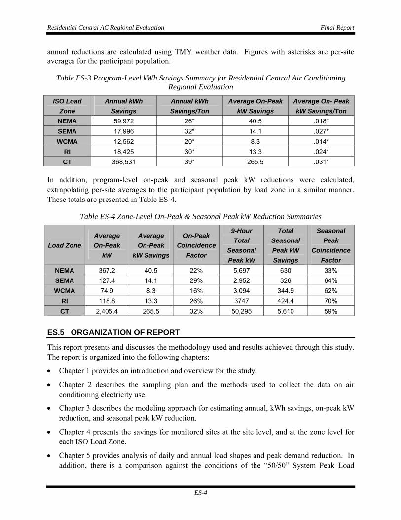
annual reductions are calculated using TMY weather data. Figures with asterisks are per-site averages for the participant population.
Table ES-3 Program-Level kWh Savings Summary for Residential Central Air Conditioning Regional Evaluation
ISO Load Zone
Annual kWh Savings
Annual kWh Savings/Ton
Average On-Peak kW Savings
Average On- Peak kW Savings/Ton
NEMA 59,972 26* 40.5 .018* SEMA 17,996 32* 14.1 .027* WCMA 12,562 20* 8.3 .014*
RI 18,425 30* 13.3 .024* CT 368,531 39* 265.5 .031*
In addition, program-level on-peak and seasonal peak kW reductions were calculated, extrapolating per-site averages to the participant population by load zone in a similar manner. These totals are presented in Table ES-4.
Table ES-4 Zone-Level On-Peak & Seasonal Peak kW Reduction Summaries
Load Zone Average On-Peak
kW
Average On-Peak
kW Savings
On-Peak Coincidence
Factor
9-Hour Total
Seasonal Peak kW
Total Seasonal Peak kW Savings
Seasonal Peak
Coincidence Factor
NEMA 367.2 40.5 22% 5,697 630 33% SEMA 127.4 14.1 29% 2,952 326 64% WCMA 74.9 8.3 16% 3,094 344.9 62%
RI 118.8 13.3 26% 3747 424.4 70% CT 2,405.4 265.5 32% 50,295 5,610 59%
ES.5 ORGANIZATION OF REPORT
This report presents and discusses the methodology used and results achieved through this study. The report is organized into the following chapters:
• Chapter 1 provides an introduction and overview for the study.
• Chapter 2 describes the sampling plan and the methods used to collect the data on air conditioning electricity use.
• Chapter 3 describes the modeling approach for estimating annual, kWh savings, on-peak kW reduction, and seasonal peak kW reduction.
• Chapter 4 presents the savings for monitored sites at the site level, and at the zone level for each ISO Load Zone.
• Chapter 5 provides analysis of daily and annual load shapes and peak demand reduction. In addition, there is a comparison against the conditions of the “50/50” System Peak Load
Residential Central AC Regional Evaluation Final Report
ES-5
Forecast, analyzing savings on days where the actual New England system load exceeded 90% of the ISO New England’s Peak Load Forecast.
• Chapter 6 contains a brief summary of and conclusions from the study.
• Appendix A contains copies of the forms used for the data collection.
• Appendix B provides further background on alternative models considered, as well as on statistical methodologies applied in this report.
• Appendix C presents input and output data used in developing the Tobit models.
• Appendix D provides graphs showing the variation in AC loads throughout the monitoring period.
• Appendix E provides predictions of load reductions for different NE ISO load zones, disaggregated by size of CAC unit.

Introduction 1-1
1. INTRODUCTION
ADM Associates, Inc. (ADM) has performed a study assessing the energy savings and demand impacts resulting from the installation of efficient central air conditioning systems (CAC) in existing and new residences. The focus of the study was on CAC systems installed through incentive programs offered to residential customers by NSTAR Electric and Gas Corporation (NSTAR), National Grid Massachusetts and Rhode Island (National Grid MA and RI), Connecticut Light & Power (CL&P), and United Illuminating (UI). This report provides and discusses the results from this study.
1.1 OVERVIEW OF STUDY METHODOLOGY
The procedures for collecting and analyzing the data for the study are described briefly, with fuller explanations of these procedures provided in subsequent chapters.
1.1.1 Data Collection The assessment of savings and load reductions was based on data collected for a sample of 96 central air conditioning units. Site-specific information (e.g., housing characteristics) was collected for each residence in the sample. In addition, ADM field staff took one-time power measurements of the new CAC unit’s compressor and air handler to determine its kW load and installed loggers to monitor indoor temperature and run time of the CAC compressor.
Information collected on the characteristics of each monitored unit included the following:
• Btu/hr. cooling capacity
• Rated unit efficiency, size, make and model of both old and replacement units
• Number of AC zones
Data on the power performance of sample units was supplemented by also taking one-time readings of the following:
• Electrical input
• Dry bulb temperatures
• Relative humidity (wet bulb temperatures)
• Supply air flow rate
Monitoring equipment was installed to measure the run time of the air conditioning system. A time-of-use motor logger was installed either in the condensing unit control compartment or in the disconnect switch box feeding the unit. By sensing the AC field generated by the current draw of the compressor, the logger could record the dates and times of each event when the compressor was turned on or off. Indoor and outdoor temperature and humidity loggers were

Residential Central AC Regional Evaluation Final Report
Introduction 1-2
used to collect data on ambient and indoor air conditions. Monitoring periods ran typically for 4-6 weeks.
1.1.2 Modeling Energy Use of CAC Units The data collected for the sample of 96 central air conditioning units were used to develop a Tobit regression model for each unit. With each unit’s regression model, hourly kW measurements were correlated to weather variables (hourly outdoor air temperatures, both dry bulb and wet bulb) over the monitoring period. Weather data for 2008 was used in developing the site-level regression models.
More detailed discussion of the specification and development of the Tobit models is provided in Section 2.3.
1.1.3 Predicting kWh Savings The Tobit1 regression model for each site was used along with Typical Meteorological Year (TMY2) weather data appropriate to a site to predict air conditioning energy use for the installed CAC system for a typical year. Following the calculation of annual energy use and load shapes for the installed system, we then calculated what energy consumption would have been had the program participant instead installed an 11 EER unit. The two sets of energy use estimates were then used to calculate kWh savings according to the following formula:
where Yi is the base case annual kWh predicted with the analytical model.3
EER is defined as
1.1.4 Analyzing Load Shapes and Predicting Peak Demand Reductions For the load shape analysis, the hourly forecasts were analyzed in order to calculate coincidence factors over on-peak periods as defined by the New England ISO: non-holiday weekdays from 1-5 PM over the months of June-August, for a total of 260 on-peak hours in the average year. These coincidence factors were defined as the percentage of available peak hours in which the compressor for the CAC system of sampled residences was running. For each ISO zone, site-
1 Tobit modeling is explained in Section 3.1 and in further detail in Appendix B.
2 The methodology for development of TMY data is explained in Section 4.1.2. 3 The model has 4,416 observations instead of 8,760 (total hours in a year) because forecast interval runs from April
15th – October 15th.
Residential Central AC Regional Evaluation Final Report
Introduction 1-3
level results were weighted by the relative occurrence of their unit size in the overall participant population. Following this, average hourly peak kW demand reductions were tabulated, as well as maximum hourly peak kW demand reductions, both totaled at the site level and at the zone level. Using this data, we also calculated Demand Reduction Values (DRVs), with this value defined as
Average DRVs were calculated using the average on-peak kW reduction values for each site.
In addition, seasonal kW reductions were calculated during hours in 2008 where the New England system load exceeded 90% of the New England ISO 50/50 System Peak Load Forecast. In 2008, there were 9 hours in which the actual system load exceeded 90% of the 50/50 System Peak Load Forecast. These hours occurred on June 9th during 2-5 PM and June 10th during noon-6 PM. kW reduction, kWh savings, and coincidence factors were calculated using the data from the monitored sites for each ISO Load Zone forecast during these hours.

Approach to Sampling and Data Collection 2-1
2. APPROACH TO SAMPLING AND DATA COLLECTION
This chapter outlines the sampling strategy employed in this study and describes the data collection procedures.
2.1 SAMPLING PLAN FOR SAVINGS ASSESSMENT
Development of the sampling plans for the project was guided by the M&V requirements set out for demand resources in ISO New England’s Manual M-MVDR1.
The M-MVDR manual specifies that the sampling requires a precision of 10% for a two tailed 80% confidence interval of an infinite population. The manual also specifies that the sample size to satisfy these precision/confidence requirements be calculated using the following equation:
2
....282.1'⎭⎬⎫
⎩⎨⎧ ×
=pr
vcn
where
n’ = number of sample points to be taken from an infinite population;
c.v. = coefficient of variation2; and
r.p = required precision
With ±10% precision at the 80% confidence level, the calculated sample size depends on the assumed coefficient of variation. Table 2-1 shows the number of sample sites required to achieve the overall sampling precision of ±10% at a confidence interval of 80% for different cv levels when this sample size formula is applied.
Table 2-1. Sample Sizes for Different Coefficients of Variation
Desired Precision
Desired Confidence
Z Value
CV Calculated
Sample Size 10% 80% 1.282 0.50 41 10% 80% 1.282 0.75 92 10% 80% 1.282 1.00 164
In the absence of known values for cv, the M-MVDR manual allows default values to be used. For non-homogeneous measures, a coefficient of variation (cv) of 1.0 is to be used. For 1 ISO New England, Inc. ISO New England Manual for Measurement and Verification of Demand Reduction Value
from Demand Resources, Revision 1, Effective Date of October 1, 2007. Sample size requirements are discussed in Section 2.1.
2 Coefficient of variation is defined as Standard Deviation / Mean. It is a normalized measure of the spread of a distribution

Residential Central AC Regional Evaluation Final Report
Approach to Sampling and Data Collection 2-2
homogeneous measures, a cv of 0.5 is acceptable for the first evaluation. However, when new sample size requirements are to be determined in subsequent evaluations, a cv calculated from previous evaluations is expected to be used.
Information about cv’s was available from similar studies of residential air conditioning.
• For a study of central air conditioning in Wisconsin conducted by the Energy Center of Wisconsin, monitoring data were collected and analyzed for a sample of 58 sites. Analysis of data from this study on CAC operating hours during days warmer than 90° F showed a cv of 0.69 for operating hours during the 3 PM to 7 PM period.
• For the coincidence factor study for residential room air conditioners in New England, it was decided that a cv of 0.75 would be a reasonable compromise for planning purposes. Under this assumption, the target sample size of sites for that study was 92.
The cv’s shown in these previous studies would indicate a sample size between 78 and 92 for this study. It was determined that a sample size of 90 or larger would allow more information to be collected with which to inform the analysis of operating hours. The monitored sample was larger than this target in order to account for possible sample attrition; in the end a sample of 96 sites was achieved.
As described in more detail below, data collected through monitoring was used to develop a regression model of CAC system hourly demand for each of the sites where monitoring of the air conditioning unit was conducted. With each unit’s regression model, hourly kW values, estimated from one time measurements of unit demand and time of use measurements for each monitored site, was correlated to hourly outdoor air temperatures (both dry bulb and wet bulb) over the monitoring period. For regression analysis, it is useful to have values for the independent variables that cover a wide range. A target sample size of 90 units made this easier to accomplish by allowing finer stratification of unit size and load zone in the sampling approach. In particular, more information could be obtained regarding the operation of central air conditioning in different load zones with different weather conditions. There are five ISO load zones (i.e., CT, RI, WCMA, SEMA, NEMA) represented among the sponsoring utilities, with somewhat different weather conditions. With a target sample of 90 units, it was possible to monitor several CAC systems in each zone. The locations of the Load Zones are shown in Figure 2-1.
2.2 SITE RECRUITMENT PROCEDURES
The target population for the monitoring sample was households in the utilities’ service territories in Massachusetts, Connecticut and Rhode Island that were participating in the utilities’ incentive programs for purchasing new CAC units. Recruitment of households to participate in the monitoring was conducted in real-time during the summer of 2008, as households signed up to participate in the utilities’ programs. Lists of households participating in the programs were provided by the utilities and / or the HVAC contractors who were installing CAC equipment through the programs.

Residential Central AC Regional Evaluation Final Report
Approach to Sampling and Data Collection 2-3
Figure 2-1. New England ISO Load Zone Map
Households that were candidates for the monitoring were contacted by telephone. The recruiters used a prepared script to inform the households of what would be required if they agreed to participate in the monitoring study. Each customer was offered an incentive payment as compensation for allowing the monitoring.
Interested customers were further screened to ensure that they fit within the specified sampling criteria specified. At the time they were called, all customers were asked questions pertaining to the characteristics of the household itself and of the new CAC unit. Questions were asked pertaining to the following:
• Household Location:
- What is your address? (street, city, zip code)
• Household Characteristics:
- How many people, including you, usually live in this home?
- How many of the people living in the house are less than 18 years in age?
- What was the highest level of education completed by the head of the household?
- What is the primary language spoken in your home?
- What range best describes your household’s total annual income?

Residential Central AC Regional Evaluation Final Report
Approach to Sampling and Data Collection 2-4
• Characteristics of HVAC unit
- How many air conditioning units does your house have?
- How many new units did you purchase?
- From which HVAC contractor did you purchase the new units?
- What is the tonnage of the new units?
- Is the unit a high efficiency unit?
This information was used to determine whether the equipment qualified for the post-installation measurements and to assign each household to an appropriate sampling stratum. Details of the stratification procedure are provided in Appendix B.
2.3 ENERGY USE MEASUREMENT PROCEDURES
Energy use measurements were made for each CAC unit in the sample. Site-specific information (e.g., characteristics of CAC unit) was collected for each residence in the sample. In addition, ADM field staff took one-time power measurements of the new CAC unit’s compressor and air handler to determine its kW load and installed loggers to monitor indoor temperature and run times of the CAC motor over the summer of 2008.
Information collected on the characteristics of each monitored CAC unit included the following:
• BTU cooling capacity
• Rated unit efficiency, size, make and model of both old and replacement units
• Number of AC zones
Some performance data on the sample units was collected by taking one-time readings of the following:
• Electrical input
• Indoor and outdoor dry bulb temperatures
• Indoor and outdoor relative humidity (wet bulb temperatures)
• Supply air flow rate
The one-time measurements were taken with the following equipment.
• An AEMC 3910 power meter was used to measure True RMS voltage, current, power and power factor. This meter has a current range from 1 to 500 A and voltage to 600V. The voltage accuracy is ±0.3%, and the current accuracy is ±2%. The voltage resolution is 1Vac, and the current resolution is 0.1 A. The power meter has a clamp-on power sensor and clip-on voltage leads.
Residential Central AC Regional Evaluation Final Report
Approach to Sampling and Data Collection 2-5
• The Sper Scientific Model 800027 RH/Temp monitor with remote sensor was used to measure temperatures and relative humidity. The dry bulb temperature range is –14ºF to 122ºF, with an accuracy of ± 2ºF from the factory and a resolution of 0.1ºF. ADM calibrated all units together for an accuracy of ± 0.5ºF. The relative humidity range is 20% to 99%, with an accuracy of ± 4% from the factory and a resolution of 1%.
For measurement of outdoor ambient conditions, a digital temperature and relative humidity meter was placed close to the unit to measure the air being drawn across the condenser coil. A radiation shield was used so that this sensor was not influenced by the sun.
The portable power meter was then clamped onto the electric line at the electric disconnect for the outside unit. The unit was then turned on and allowed to run for at least ten minutes for the refrigeration cycle to stabilize. This measurement captures the compressor and condenser fan kW draw.
Monitoring equipment was also installed to measure the run time of the air conditioning system. Time-of-use motor loggers manufactured by Onset Computers were used to collect run time measurements. The logger was installed either in the condensing unit control compartment or in the disconnect switch box feeding the unit. By sensing the ac field generated by the current draw of the compressor, the logger could record the dates and times of each event when the compressor was turned on or off. The time-of-use loggers used have 26K of memory, which was enough to hold measurements made during an entire summer of A/C compressor cycling.
Indoor and outdoor temperature and humidity loggers manufactured by Onset Computers were used to collect data on ambient and indoor air conditions.
2.4 PREPARING LOAD DATA FOR ANALYSIS
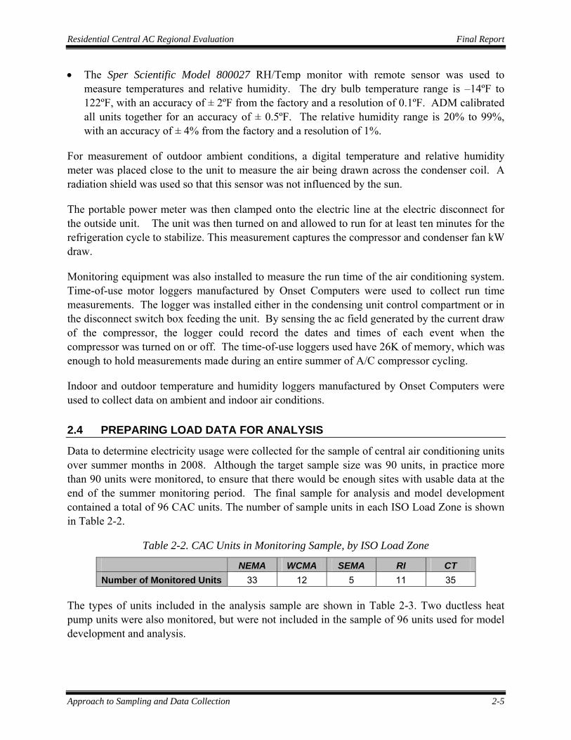
Data to determine electricity usage were collected for the sample of central air conditioning units over summer months in 2008. Although the target sample size was 90 units, in practice more than 90 units were monitored, to ensure that there would be enough sites with usable data at the end of the summer monitoring period. The final sample for analysis and model development contained a total of 96 CAC units. The number of sample units in each ISO Load Zone is shown in Table 2-2.
Table 2-2. CAC Units in Monitoring Sample, by ISO Load Zone
NEMA WCMA SEMA RI CT Number of Monitored Units 33 12 5 11 35
The types of units included in the analysis sample are shown in Table 2-3. Two ductless heat pump units were also monitored, but were not included in the sample of 96 units used for model development and analysis.
Residential Central AC Regional Evaluation Final Report
Approach to Sampling and Data Collection 2-6
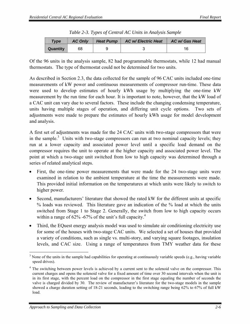
Table 2-3. Types of Central AC Units in Analysis Sample
Type AC Only Heat Pump AC w/ Electric Heat AC w/ Gas Heat
Quantity 68 9 3 16
Of the 96 units in the analysis sample, 82 had programmable thermostats, while 12 had manual thermostats. The type of thermostat could not be determined for two units.
As described in Section 2.3, the data collected for the sample of 96 CAC units included one-time measurements of kW power and continuous measurements of compressor run-time. These data were used to develop estimates of hourly kWh usage by multiplying the one-time kW measurement by the run time for each hour. It is important to note, however, that the kW load of a CAC unit can vary due to several factors. These include the changing condensing temperature, units having multiple stages of operation, and differing unit cycle options. Two sets of adjustments were made to prepare the estimates of hourly kWh usage for model development and analysis.
A first set of adjustments was made for the 24 CAC units with two-stage compressors that were in the sample.3 Units with two-stage compressors can run at two nominal capacity levels; they run at a lower capacity and associated power level until a specific load demand on the compressor requires the unit to operate at the higher capacity and associated power level. The point at which a two-stage unit switched from low to high capacity was determined through a series of related analytical steps.
• First, the one-time power measurements that were made for the 24 two-stage units were examined in relation to the ambient temperature at the time the measurements were made. This provided initial information on the temperatures at which units were likely to switch to higher power.
• Second, manufacturers’ literature that showed the rated kW for the different units at specific % loads was reviewed. This literature gave an indication of the % load at which the units switched from Stage 1 to Stage 2. Generally, the switch from low to high capacity occurs within a range of 62% -67% of the unit’s full capacity.4
• Third, the EQuest energy analysis model was used to simulate air conditioning electricity use for some of the houses with two-stage CAC units. We selected a set of houses that provided a variety of conditions, such as single vs. multi-story, and varying square footages, insulation levels, and CAC size. Using a range of temperatures from TMY weather data for these
3 None of the units in the sample had capabilities for operating at continuously variable speeds (e.g., having variable
speed drives). 4 The switching between power levels is achieved by a current sent to the solenoid valve on the compressor. This
current charges and opens the solenoid valve for a fixed amount of time over 30 second intervals when the unit is in its first stage, with the percent load on the compressor in the first stage equaling the number of seconds the valve is charged divided by 30. The review of manufacturer’s literature for the two-stage models in the sample showed a charge duration setting of 18-21 seconds, leading to the switching range being 62% to 67% of full kW load.

Residential Central AC Regional Evaluation Final Report
Approach to Sampling and Data Collection 2-7
simulations provided data with which to calculate the relationship between cooling loads (as measured in tons) and dry bulb temperatures. This relationship, combined with information on individual units’ capacities (in tons), was then used to estimate at what outside temperature each unit would switch from Stage 1 to Stage 2 for cooling. The monitoring data was analyzed to determine when the temperature exceeded the threshold for the unit to enter its second stage by examining both the outside temperature and the size of the sampled residence’s CAC unit. The temperature thresholds for various tonnages are detailed in Appendix B.
• Whether the one-time power measurement was for the first-stage or second-stage was determined by examining the kW/ton values for each CAC unit, normalized for size and EER ratings. This provided two distinct groupings.
In a second set of adjustments, the hourly kWh estimates were adjusted based on changes in outside temperature. CAC efficiency declines as temperature increases, causing the kW draw of the unit to vary with outside temperature. To account for this, changes in kW were made to reflect temperature changes. Each sampled unit had an individual baseline for this calculation, determined by the ambient temperature that was recorded during the one-time power reading while onsite. The kW reading for a unit was increased by 1% for each degree increase in ambient temperature relative to the ambient temperature when the one-time power measurement was recorded5. This adjustment factor is based on prior studies analyzing weather impacts on CAC efficiency. For two-stage units, this adjustment was made after adjusting for staging.
This adjustment procedure is displayed in the following formula:
where
for a given hour i. Tempi figures were from the 2008 weather data for the weather station nearest to the residence during model development. The 1% degree deviation adjustment accounts for seasonal changes in a way that EER alone cannot, as it is a measure of efficiency at 95 degrees F. By adjusting the kW draw based on outside temperature, the seasonal efficiency of a CAC is calculated for every hour of data analyzed.
5 For example, see Neal and O’Neal, “The Impact of Residential Air Conditioner Charging and Sizing on Peak
Electrical Demand”, ACEEE 1992 Summer Study of Energy Efficiency in Buildings, 1992, pp. 2.189-2.200. For an example of empirical data showing the relationship between kW and ambient temperature, see KEMA, Pacific Gas & Electric SmartAC™ 2008 Residential ExPost Load Impact Evaluation and Ex Ante Load Impact Estimates, Final Report, March 31, 2009, pp. 5-1.

Residential Central AC Regional Evaluation Final Report
Approach to Sampling and Data Collection 2-8
Information with which to calculate percent time on for a given period was obtained through examination of the motor logger data from the compressor. In HOBO motor logger data, a value of 1 indicates the compressor switching on and a zero indicates the compressor switching off. The total time in each hour between a 1 value and a zero value was summed to calculate total minutes on in a given hour, and then divided by 60 for the percent time on value. From this, total kWh over the forecast period was calculated as:

Modeling Site-Level Air Conditioning Energy Use 3-1
3. MODELING SITE-LEVEL AIR CONDITIONING ENERGY USE
This chapter discusses the development of site-level models for predicting air conditioning energy use. Further detail pertaining to alternative model specifications and tests of the models and the data used are provided in Appendix B.
3.1 MODEL SPECIFICATION ISSUES
As a general specification, it was expected that site-level models for predicting air conditioning energy use would relate measured energy use to such explanatory variables as dry and wet bulb temperatures. However, the particular specification used for the site-level models needed to take account of the fact that the monitoring data collected for the CAC units in the study sample showed that there were significant numbers of hours for most units in which the compressor was not running (i.e., there was no energy use for the compressor in those hours). It is possible that the CAC fan could be running while the compressor is off, but during such times, no savings would be realized, as the savings from high-efficiency CACs are attributable to more efficient compressors.
With a site-specific data set showing significant numbers of zero values for energy use, estimating a relationship between energy use and the driving weather variables through ordinary least squares (OLS) regression would produce inconsistent estimates for the model coefficients. The OLS estimates for slope coefficients would understate the true slope coefficients, depending on the fraction of data points that have non-zero values. That is, the inconsistency of the coefficients estimated with OLS regression becomes greater, the larger the number of zero energy use values there are in the data set for a unit.
To address the problem that zero energy use values creates for estimating site-specific models, we used a Tobit estimation model for each unit within the sample. Tobit modeling for estimation of energy use has been used in several prior studies1. This methodology has also been applied in papers from the International Association of Energy Economics (IAEE.org) for models of energy pricing and consumption.
The Tobit model is a method of correcting for data that is top or bottom censored, i.e., data that either due to physical or practical limitations has a floor or ceiling on its range and also displays a high concentration of data points at the censored boundary. It does so by means of an intermediate step in which values of the dependent variable are temporarily allowed to breach their censoring guideline. In the case at hand, this means allowing for energy use values to be
1 For examples, see the following:
Lucas, W. Davis, “Durable Goods and Residential Demand for Energy and Water: Evidence From a Field Trial”, RAND Journal of Economics, Vol. 39, No. 2, Summer 2008, pp. 530–546.
KEMA, Final Report, Pacific Gas and Electric SmartAC Load Impact Evaluation, Prepared for Pacific Gas and Electric Company, April 24, 2008.

Residential Central AC Regional Evaluation Final Report
Modeling Site-Level Air Conditioning Energy Use 3-2
negative. In doing so, the Tobit estimation procedure corrects the estimation of points where energy use is positive. In effect, a high proportion of zero values in the data set no longer biases the slope coefficients downward.
The contrast between using the Tobit modeling procedure and the OLS regression procedures can be illustrated with Figures 3-1 and 3-2. In the two figures, all positive values of kWh are identical. In Figure 3-1, temperatures where the CAC unit is not running are shown as zero kWh. In Figure 3-2, the intermediate step in the Tobit model is shown. The values that previously equaled zero are predicted to be negative, allowing for more accurate predictions at dry bulb temperatures where kWh values are positive. When the Tobit correction for censored values is implemented, the slope increases, the intercept increases, and predicted kWh become more weather-dependent. For this example illustration, the R2 of the fitted model increased from 69.6% for the OLS regression model in Figure 3-1 to 85.8% for the Tobit model in Figure 3-2. Extrapolated out to a full summer cooling season, a site-specific model developed through the Tobit modeling procedure will be more precise for hours when energy use is positive.
Figure 3-1. OLS Regression Energy Use Prediction Model with Values Censored at Zero

Residential Central AC Regional Evaluation Final Report
Modeling Site-Level Air Conditioning Energy Use 3-3
Figure 3-2. Tobit Energy Use Prediction Model with No Censored Values
Another option for modeling residential CAC use was fixed effects modeling, where all sites are combined into one regression with a dummy variable representing each individual site. We opted for site-specific Tobit models instead of fixed-effects for a variety of reasons. First, with fixed effect modeling, each CAC unit would be assumed to have the same weather response coefficients once the dummies for individuals and time periods are accounted for. However, that may provide an inaccurate depiction of responses to weather changes, as the only site-specific factor it accommodates is the tipping point where the CAC unit begins running, averaging out differences in magnitude of reaction. This contrasts with what is observed in the monitored data, in that the responses to weather changes after the tipping point has been reached for individual units can vary widely
3.2 DEVELOPMENT OF SITE-SPECIFIC TOBIT MODELS
This section presents and discusses the development of the site-specific Tobit models.
3.2.1 Tobit Modeling Specification The general specification used for the Tobit modeling was as follows:
The censored dependent variable Yi is defined as

Residential Central AC Regional Evaluation Final Report
Modeling Site-Level Air Conditioning Energy Use 3-4
where εi is a normal error term with zero mean and standard deviation σ, calculated as
Once the model was estimated for the existing data for a site, model fit was assessed by first calculating hourly usage values over the observation period for that site, using the estimated coefficients and the actual temperature and other data. The calculated in-sample values were then tested for their squared correlation coefficient with the actual kWh values. This provided a readily interpretable facsimile for the R2 values provided in OLS estimations. In addition, all predictions were checked for mean biasing2 in the estimate. These checks confirmed that mean biasing in predicted kW was minimal, with less than 2% deviation in mean kWh use between predicted and monitored data.
The Tobit model specification used fits estimates according to a normal distribution. Several other distributions were tested and compared, including Beta, logistic, Gamma, Weibull, log-logistic, extreme value, and exponential distributions. However, the normal distribution was chosen as it provided a superior log-likelihood value relative to these other distributions.
The dependent variable for the Tobit models was either the unadjusted or the adjusted hourly kWh usage values. The savings totals presented in this report are the result of models that incorporated adjusted kWh values. Totals with raw kWh values were calculated for purposes of comparison. The variables listed in Table 3-1 were used as independent variables in the estimation of the site-specific Tobit models. The actual estimation of the models was accomplished using the Statistical Analysis System (SAS) software package3.
To prevent multicollinearity (i.e., where one independent variable is a linear function of one or more other independent variables), morning variables and associated interaction terms were excluded from the regressions. As such, values for the morning period are defined as when afternoon and night = 0. In addition, though we have data for relative humidity, it is not included in the model, as it is a function of dry and wet bulb temperatures.
2 Mean Biasing is defined as when the mean of kWh values calculated from the regression differs from the mean of
actual monitored kWh. The models’ calculated means were the same as monitored (within a few percentage points) but with a larger standard deviation.
3 The SAS modeling code for Tobit estimation is provided in Appendix B.

Residential Central AC Regional Evaluation Final Report
Modeling Site-Level Air Conditioning Energy Use 3-5
Table 3-1. Descriptions of Variables Used in Estimation of Tobit Models
Variable Name Description kWh Kilowatt hours estimates on hourly intervals.
Calculated via one-hour averaging of 5 minute data. kWh_adj Kilowatt hours estimates on hourly intervals adjusted by 1% per degree deviation
from reference temperature. Temp_db Dry bulb temperature
Temp_wb Wet bulb temperature
Lagged_Temp_db 3 - period weighted moving average of dry bulb temperature
Lagged_Temp_wb 3 - period weighted moving average of wet bulb temperature
Heatwave_db 24 hour lag term for dry bulb temperature
Heatwave_wb 24 hour lag term for wet bulb temperature
Morning Dummy indicating the hours of 12:00 AM – 12:00 PM
Afternoon Dummy indicating the hours of 12:00 PM – 8:00 PM
AfternoonTempDB Afternoon*Temp_db
AfternoonTempWB Afternoon*Temp_wb
AfternoonLagTempDB Afternoon*Lagged_Temp_db
AfternoonLagTempWB Afternoon*Lagged_Temp_wb
AfternoonHeatwave_db Afternoon*Heatwave_db
AfternoonHeatwave_wb Afternoon*Heatwave_wb
Night Dummy indicating the hours of 8:00 PM – 12:00 AM
NightTempDB Night*Temp_db
NightTempWB Night*Temp_wb
NightLagTempDB Night*Lagged_Temp_db
NightLagTempWB Night*Lagged_ Temp_wb
NightHeatwave_db Night*Heatwave_db
NightHeatwave_wb Night*Heatwave_wb
Weekend Dummy indicating observations on Saturday or Sunday
WeekendTempDB Weekend*Temp_db
WeekendTempWB Weekend*Temp_wb
WeekendLagTempDB Weekend*Lagged_ Temp_db
WeekendLagTempWB Weekend*Lagged_ Temp_wb
WeekendHeatwave_db Weekend*Heatwave_db
WeekendHeatwave_wb Weekend*Heatwave_wb
Scale Standard error of the Tobit regression
3.2.2 Lag Weighting Schemes for Tobit Models For the modeling, lag terms were included, where “lag” term refers to how many hours behind the current hour the term is, with Lag-1 being one hour behind, etc. For residential CAC use, the previous hour(s)’ temperature can significantly affect current hour usage by buildup of thermal inertia, with the residence retaining heat from prior hot hours. For this study, three previous
Residential Central AC Regional Evaluation Final Report
Modeling Site-Level Air Conditioning Energy Use 3-6
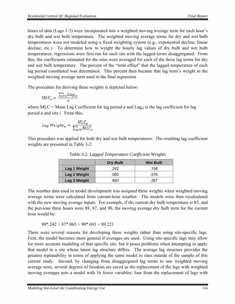
hours of data (Lags 1-3) were incorporated into a weighted moving average term for each hour’s dry bulb and wet bulb temperature. The weighted moving average terms for dry and wet bulb temperatures were not modeled using a fixed weighting system (e.g., exponential decline, linear decline, etc.). To determine how to weight the hourly lag values of dry bulb and wet bulb temperatures, regressions were first run for each site with the lagged terms disaggregated. From this, the coefficients estimated for the sites were averaged for each of the three lag terms for dry and wet bulb temperature. The percent of the “total effect” that the lagged temperature of each lag period constituted was determined. This percent then became that lag term’s weight in the weighted moving average term used in the final regression.
The procedure for deriving these weights is depicted below:
where MLC = Mean Lag Coefficient for lag period a and Lagai is the lag coefficient for lag period a and site i. From this,
This procedure was applied for both dry and wet bulb temperatures. The resulting lag coefficient weights are presented in Table 3-2.
Table 3-2. Lagged Temperature Coefficient Weights
Dry Bulb Wet Bulb Lag 1 Weight .242 .158 Lag 2 Weight .065 .576 Lag 3 Weight .693 .267
The weather data used in model development was assigned these weights when weighted moving average terms were calculated from current-hour weather. The models were then recalculated with the new moving average inputs. For example, if the current dry bulb temperature is 85, and the previous three hours were 88, 87, and 90, the moving average dry bulb term for the current hour would be:
88*.242 + 87*.065 + 90*.693 = 89.221
There were several reasons for developing these weights rather than using site-specific lags. First, the model becomes more general if averages are used. Using site-specific lags may allow for more accurate modeling of that specific site, but it poses problems when attempting to apply that model to a site whose latent lag structure differs. The average lag structure provides the greatest repeatability in terms of applying the same model to sites outside of the sample of this current study. Second, by changing from disaggregated lag terms to one weighted moving average term, several degrees of freedom are saved as the replacement of the lags with weighted moving averages nets a model with 16 fewer variables: four from the replacement of lags with

Residential Central AC Regional Evaluation Final Report
Modeling Site-Level Air Conditioning Energy Use 3-7
moving averages (remove six lags, add two moving averages) and the remaining 12 from the removal of associated interaction terms with the afternoon, night, and weekend dummy variables.
3.2.3 Summary of Estimation Results for Tobit Modeling Table 4-3 summarizes the results from estimation of the Tobit models. (Full results from the estimation of the Tobit models are provided in Appendix C.) In Table 3-3, the columns display the percentage of monitored sites where the variable for that row was significant at the level specified in the column heading. The 10% column is cumulative; it includes sites significant at the 5% level in its tally.
Table 3-3. Significance Rates for Model Variables
Variable Name Percent of Sites
Significant at 5% Level
Percent of Sites Significant at
10% Level Intercept 84% 89% Weekend 38% 45% Weekendtempdb 20% 24% Weekendtempwb 8% 15% WeekendLagTempDB 22% 29% WeekendLagTempWB 15% 25% Temp_db 40% 47% Temp_wb 11% 23% Lagged_Temp_db 38% 48% Lagged_Temp_wb 11% 16% Night 31% 39% nightTempdb 19% 28% nightTempwb 11% 18% NightLagTempDB 27% 34% NightLagTempWB 9% 15% Afternoon 34% 41% afternoonTempdb 22% 32% afternoonTempwb 9% 18% AfternoonLagTempDB 24% 32% AfternoonLagTempWB 15% 25% Heatwave_db 27% 35% Heatwave_wb 38% 42% afternoonheatwave_db 23% 34% afternoonheatwave_wb 25% 30% Nightheatwave_db 16% 23% Nightheatwave_wb 13% 18%

Residential Central AC Regional Evaluation Final Report
Modeling Site-Level Air Conditioning Energy Use 3-8
Further information on the development of the Tobit models, including comparisons to alternative specifications, is provided in Appendix B.
Savings Predictions 4-1
4. SAVINGS PREDICTIONS
This chapter presents both site-level and zone-level predictions for annual kWh savings and on- peak kW reductions. In addition, estimates are presented of seasonal peak savings, where total system load exceeds 90% of the New England ISO 50/50 System Peak Forecast for 2008.
The model for each site applies a set of rules to hourly data on weather, time of day, and associated interactions to compute a prediction of hourly kWh. Each predicted hourly kWh is multiplied by the appropriate weight associated with that CAC unit in the microdata file. The weighted individual results are then added together to obtain the aggregate result.
4.1 PREDICTING LOADS WITH SITE-SPECIFIC TOBIT MODELS
For each sample site, the Tobit model specific to that site was used to calculate predictions of air conditioning loads. Two sets of predictions were developed, one using Typical Meteorological Year (TMY) data for a weather station representative of an applicable Load Zone and the other using actual 2008 weather data. Both the site-specific prediction procedure and the weather data that were used are discussed in this section.
4.1.1 Site-Specific Prediction Procedure Tobit Estimation was used to get hourly predictions of kW based on outside temperature. For details of calculating Tobit predictions, refer to Appendix B.
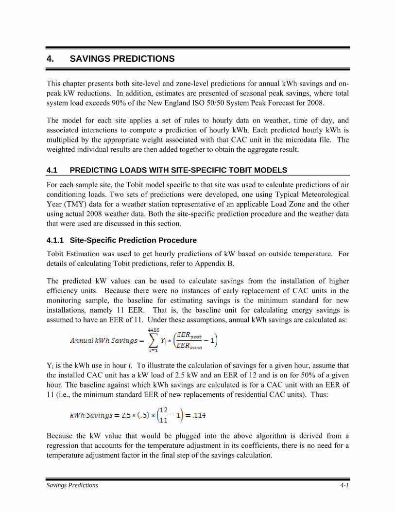
The predicted kW values can be used to calculate savings from the installation of higher efficiency units. Because there were no instances of early replacement of CAC units in the monitoring sample, the baseline for estimating savings is the minimum standard for new installations, namely 11 EER. That is, the baseline unit for calculating energy savings is assumed to have an EER of 11. Under these assumptions, annual kWh savings are calculated as:
Yi is the kWh use in hour i. To illustrate the calculation of savings for a given hour, assume that the installed CAC unit has a kW load of 2.5 kW and an EER of 12 and is on for 50% of a given hour. The baseline against which kWh savings are calculated is for a CAC unit with an EER of 11 (i.e., the minimum standard EER of new replacements of residential CAC units). Thus:
Because the kW value that would be plugged into the above algorithm is derived from a regression that accounts for the temperature adjustment in its coefficients, there is no need for a temperature adjustment factor in the final step of the savings calculation.
Residential Central AC Regional Evaluation Final Report
Savings Predictions 4-2
4.1.2 Weather Data Used for Predicting Site-Specific AC Loads Two sets of weather data were used in preparing predictions of site-specific air conditioning loads.
• Typical Meteorological Year (TMY) data for New England weather stations were used to develop predictions of kWh usage and savings.
• Actual weather data for 2008 were used to develop predictions of peak day loads and load reductions.
Typical Meteorological Year (TMY) weather data are prepared using various meteorological measurements made at hourly intervals over a number of years to build up a picture of the local climate. A simple average of the yearly data underestimates the amount of variability, so the month that is most representative of the location is selected. For each month, the average temperature over the whole measurement period is determined, together with the average temperature in each month during the measurement period. The data for the month that has the average temperature most closely equal to the monthly average over the whole measurement period is then chosen as the TMY data for that month. This process is then repeated for each month in the year. The months are joined together to give a full year of hourly weather data.
Two sets of TMY data for locations in the United States have been produced by the National Renewable Energy Laboratory's (NREL's) Analytic Studies Division under the Resource Assessment Program, which is funded and monitored by the U.S. Department of Energy's Office of Solar Energy Conversion.
• TMY2 data sets are derived from the 1961-1990 National Solar Radiation Data Base (NSRDB).
• TMY3 data are derived from data for a 1991-2005 period of record.
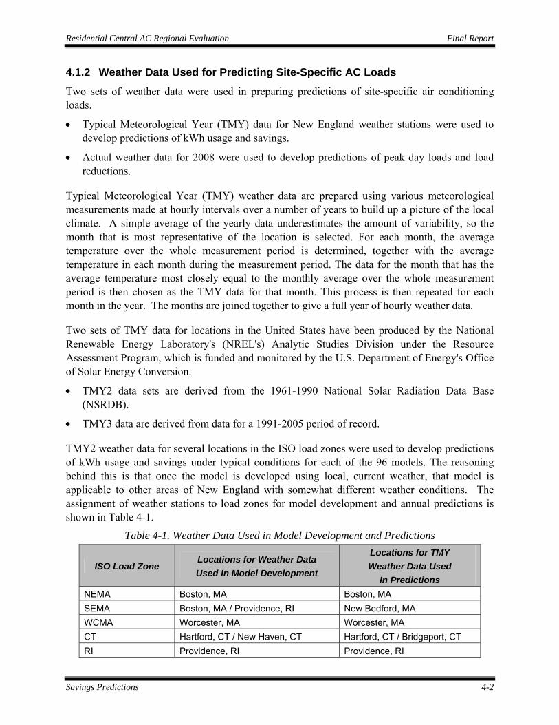
TMY2 weather data for several locations in the ISO load zones were used to develop predictions of kWh usage and savings under typical conditions for each of the 96 models. The reasoning behind this is that once the model is developed using local, current weather, that model is applicable to other areas of New England with somewhat different weather conditions. The assignment of weather stations to load zones for model development and annual predictions is shown in Table 4-1.
Table 4-1. Weather Data Used in Model Development and Predictions
ISO Load Zone Locations for Weather Data Used In Model Development
Locations for TMY Weather Data Used
In Predictions NEMA Boston, MA Boston, MA SEMA Boston, MA / Providence, RI New Bedford, MA WCMA Worcester, MA Worcester, MA CT Hartford, CT / New Haven, CT Hartford, CT / Bridgeport, CT RI Providence, RI Providence, RI
Residential Central AC Regional Evaluation Final Report
Savings Predictions 4-3
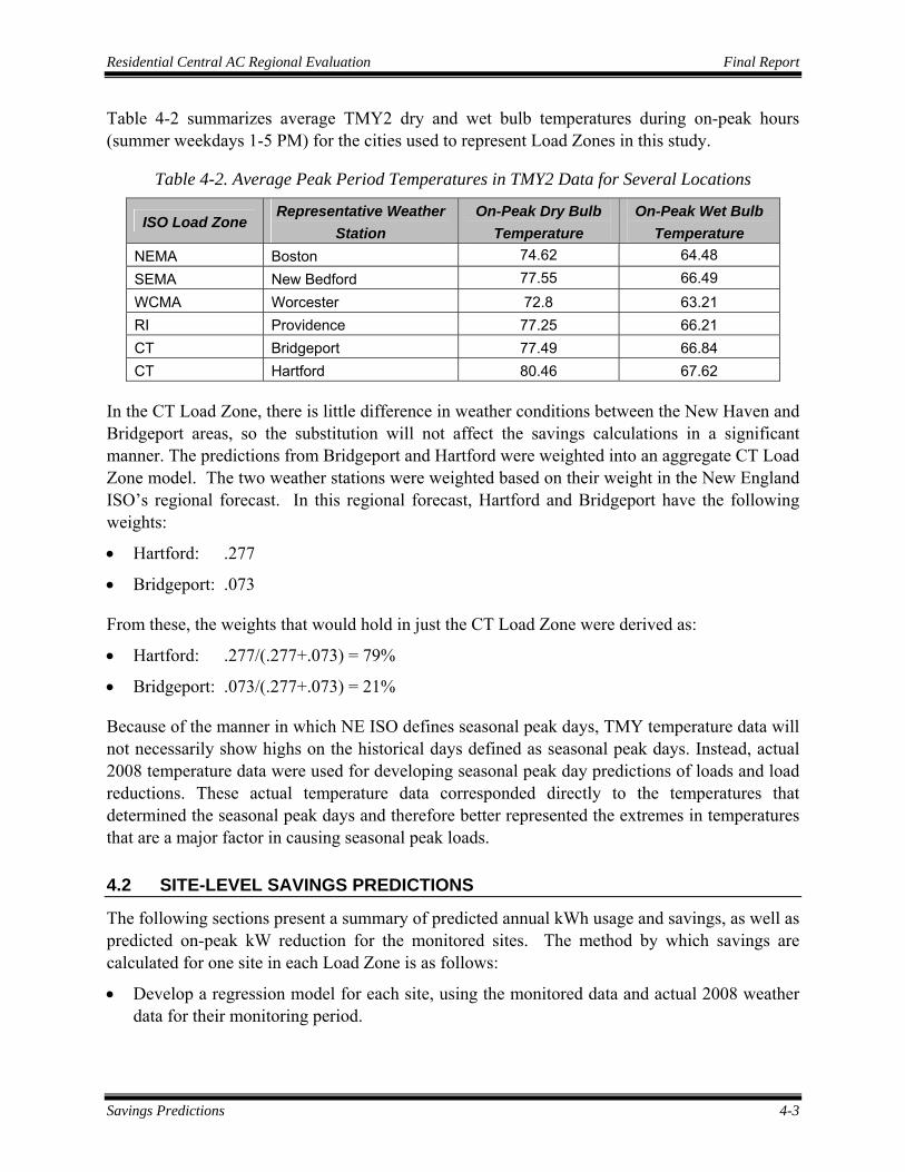
Table 4-2 summarizes average TMY2 dry and wet bulb temperatures during on-peak hours (summer weekdays 1-5 PM) for the cities used to represent Load Zones in this study.
Table 4-2. Average Peak Period Temperatures in TMY2 Data for Several Locations
ISO Load Zone Representative Weather
Station On-Peak Dry Bulb
Temperature On-Peak Wet Bulb
Temperature NEMA Boston 74.62 64.48 SEMA New Bedford 77.55 66.49 WCMA Worcester 72.8 63.21 RI Providence 77.25 66.21 CT Bridgeport 77.49 66.84 CT Hartford 80.46 67.62
In the CT Load Zone, there is little difference in weather conditions between the New Haven and Bridgeport areas, so the substitution will not affect the savings calculations in a significant manner. The predictions from Bridgeport and Hartford were weighted into an aggregate CT Load Zone model. The two weather stations were weighted based on their weight in the New England ISO’s regional forecast. In this regional forecast, Hartford and Bridgeport have the following weights:
• Hartford: .277
• Bridgeport: .073
From these, the weights that would hold in just the CT Load Zone were derived as:
• Hartford: .277/(.277+.073) = 79%
• Bridgeport: .073/(.277+.073) = 21%
Because of the manner in which NE ISO defines seasonal peak days, TMY temperature data will not necessarily show highs on the historical days defined as seasonal peak days. Instead, actual 2008 temperature data were used for developing seasonal peak day predictions of loads and load reductions. These actual temperature data corresponded directly to the temperatures that determined the seasonal peak days and therefore better represented the extremes in temperatures that are a major factor in causing seasonal peak loads.
4.2 SITE-LEVEL SAVINGS PREDICTIONS
The following sections present a summary of predicted annual kWh usage and savings, as well as predicted on-peak kW reduction for the monitored sites. The method by which savings are calculated for one site in each Load Zone is as follows:
• Develop a regression model for each site, using the monitored data and actual 2008 weather data for their monitoring period.

Residential Central AC Regional Evaluation Final Report
Savings Predictions 4-4
• Collect TMY2 data for each Load Zone, with this encompassing data from the following locations: - Boston, MA - New Bedford, MA - Worcester, MA - Providence, RI - Hartford, CT - Bridgeport, CT
• Apply the data from each of the above cities to the regression model for the site, giving energy use calculations for all five Load Zones
As a result, 96 predictions are made for each ISO Load Zone. The predictions are made using site-specific coefficients (based on analysis of the past) for weather variables, but (to predict future savings) applied to standardized weather data from one load zone at a time. Thus, the 96 sets of coefficients are used five times each, once for each load zone. At the site level, this presumes that the Load Zones differ only in weather, and not in other fundamental characteristics.
4.2.1 Site-Level Annual Savings by ISO Load Zone This section provides the results of an analysis of annual savings from the Tobit models, using each of the 96 CAC units in the sample. The savings figures presented in this section are calculated using Typical Meteorological Year Data (TMY) in order to generalize the estimated savings to a typical future cooling season. Table 4-3 provides these summaries by ISO Load Zone, with average annual savings for monitored sites, as well as savings per ton. Within each load zone, savings are subdivided by the sizes of the CAC units in the sample. All numbers in the tables are given in terms of per-site averages, derived from applying the weather from each load zone to all 96 sites. The actual distribution of sizes for the 96 monitored sites is identical across the five load zones.
Table 4-3. Annual Savings by Load Zone, for Average Site
Annual kWh Usage
Annual kWh Savings
Annual kWh Savings/Ton
Equivalent Full Load Operating hours
NEMA 629 71 25 302 SEMA 851 95 34 407 WCMA 504 57 20 244
RI 778 87 31 372 CT 992 111 40 475

Residential Central AC Regional Evaluation Final Report
Savings Predictions 4-5
In Table 4-3, the terms denoted in the columns are defined as:
The weighted average connected load refers to the kW load of the CAC units weighted by the annual kWh values. The figures in this column represent the average number of hours that the CAC compressor runs annually.
Tables E-1 thru E-5 in Appendix E provide summaries for each Load Zone broken down by unit size (tons). On the site level, there is significant variation in annual use, to a degree which could not fully be accounted for in sample design. There are a number of reasons to account for the variations across sample sites. First, there were a significant number of program participants that were installing a CAC unit at their home for the first time. As such, usage for these homes could not be determined a priori during sample development. This resulted in an error in stratification during sampling, as program participants were stratified by service territory (as a proxy for load zone) and prior use. Without any prior use to compare against, there was no certain way to determine the proper strata for first-time CAC users. However, given the significant portion of the program participant database that this class of users consists of, it would have been inappropriate to exclude them. The findings showed that individuals that installed their first CAC as part of this program were among the infrequent users. Such users are likely accustomed to alternate methods of comfort during the peak cooling season (e.g., using fans, opening windows, etc.).
4.2.2 Site-Level On-Peak Savings by ISO Load Zone Table 4-4 presents the site-level on-peak savings estimates for the 96 sampled sites. As with the annual savings calculations, the on-peak savings calculations are derived from applying TMY weather data from each ISO Load Zone to each of the 96 regression models, providing a sample of 96 households for each Load Zone. The ISO-defined on-peak period includes all non-holiday weekdays in the months of June-August from 1:00 – 5:00 PM. The terms denoting each column in Table 4-4 are defined as follows:

Residential Central AC Regional Evaluation Final Report
Savings Predictions 4-6
Table 4-4. On-Peak Savings by Load Zone, for Average Site
On-Peak kWh
On-Peak kWh
Savings
Average On-Peak
kW
Average On-Peak
kW Savings
Average On-Peak
kW Savings / Ton Per
Unit
Maximum On-Peak
kW
Maximum On-Peak
kW Savings
NEMA 109 12.3 .42 .047 .017 1.48 .168 SEMA 167 18.8 .642 .072 .025 2.15 .244 WCMA 84 9.5 .323 .037 .013 1.58 .179
RI 142 16.1 .55 .060 .022 1.89 .210 CT 182 20.5 .699 .079 .029 2.01 .227
Tables E-6 through E-10 in Appendix E provide summaries for each Load Zone broken down by unit size (tons).
4.3 AGGREGATION FOR ZONE-LEVEL SAVINGS
This section presents estimates of the aggregated savings by ISO Load Zone. The procedure for estimating aggregate savings is described first. Estimates of total annual kWh savings are then presented, followed by estimates of on-peak kW reductions for all program participants in each ISO Load Zone.
4.3.1 Procedure to Estimate Aggregate Savings Zone-level aggregate results were obtained by weighting the sample sites by size and efficiency according to how CAC units installed in a zone through the Sponsors’ programs were distributed. Essentially, the sample of 96 units was reweighted for each zone to be representative of that zone’s population of newly installed CAC units. These weights were determined by using the data from the tracking systems for the utilities’ CAC programs to determine the load zone for each participant. For some load zones, there could be program participants from several of the programs (e.g., NSTAR and National Grid MA could each have program participants in SEMA).
In order to determine the weighting, the distribution of program units in each load zone needed to be determined. To this end, program tracking data provided by utilities were used to tally the number of units in each size category within each load zone. The mean value for each hourly

Residential Central AC Regional Evaluation Final Report
Savings Predictions 4-7
prediction was calculated for each size category in the sample and the average for each category was then multiplied by the number of units in that size category in the load zone population.
Table 4-5 shows the percentage distributions of CAC units by size for each ISO load zone. The monitoring sample did not include any 1-ton or 4.5-ton units, and had only 2 1.5-ton and 1 5-ton unit. As such, the 1, 1.5, and 2-ton classes were aggregated for each load zone. In addition, the 4, 4.5, and 5-ton categories were aggregated as well. One-, 4.5- and 5-ton units made up a small percentage of the total participation, so statistically significant sampling of each of the categories would be inefficient.
Table 4-5. Percentage Representation of CAC Units by Size by Load Zone
Unit Size NEMA SEMA WCMA RI CT % of Sample
1 4.8% 2.0% 5.2% 3.2% 6.7% .00% 1.5 5.3% 5.6% 11.7% 14.0% 7.5% 2.08% 2 17.7% 25.5% 20.0% 18.5% 24.0% 27.08%
2.5 18.0% 22.4% 21.7% 23.0% 14.5% 18.75% 3 31.9% 25.0% 23.9% 27.9% 27.5% 39.58%
3.5 7.1% 9.2% 5.7% 3.6% 4.2% 4.17% 4 10.6% 5.6% 10.0% 9.0% 12.5% 7.29%
4.5 0.6% 1.0% 0.4% 0.5% 0.4% .00% 5 3.9% 3.6% 1.3% 0.5% 2.6% 1.04%
Total Number of Units
790 196 230 222 3,269 96
An example illustrates the weighting procedure for annual kWh for the NEMA Load Zone, with explicit calculation for one CAC size:
1. Determine the per-site average annual kWh for a CAC size in a given load zone. For this example, consider 3-ton CAC units in the NEMA Load Zone. The average annual kWh for 3-Ton CAC units in NEMA is 724.49 (Table E-6 shows this value rounded to 724).
2. Determine the number of 3-ton units in the NEMA Load Zone. According to Table 4-6, there are 252 3-ton CACs in the NEMA Load Zone for the entire program.
3. Multiply these two factors: 724.49 * 252 = 182,571 (as shown in the Total Annual kWh column in Table E-11).
An extra step is required for the top and bottom size categories, as these are aggregated across unit sizes. For an example of the 1-1.5-2 ton aggregated class in the NEMA Load Zone:
1. Calculate total kWh for the monitored sites in each class: 545.4 for 1.5-ton, 366.6 for 2-ton (Values in Table E-1 rounded). These figures are calculated by multiplying the per-

Residential Central AC Regional Evaluation Final Report
Savings Predictions 4-8
site kWh averages in Table E-1 by the number of sampled sites in each size category (2 1.5-ton and 26 2-ton). - 1.5 Ton: 2 * 545.4 = 1,090.8 - 2 Ton: 26 *366.6 = 9,531.6
2. Divide the sum of these numbers by the total number of 1.5 and 2 ton monitored sites (28): 10,622.4/28 = 379.37
3. Multiply this by the total number of 1, 1.5, and 2-ton units in the NEMA Load Zone: 379.37*220 = 83,458 (shown in Table E-11)
These procedures are repeated for each size class (applying the cross-class aggregation where necessary). The results are then summed or averaged where applicable in order to provide zone-level summary statistics.
4.3.2 Predicted Zone-Level Total kWh Savings The participation by unit size for each Load Zone are detailed in Table 4-6. The CT Load Zone had the highest participation across the five load zones in this study, and consequently shows the highest kWh savings. The higher participation, coupled with warmer weather in the CT Load Zone relative to other load zones in this study, leads to high CAC energy use.
Table 4-6. Participants in Utility Programs by Load Zone
Unit Size NEMA SEMA WCMA RI CT
1 38 4 12 7 220 1.5 42 11 27 31 246 2 140 50 46 41 785
2.5 142 44 50 51 474 3 252 49 55 62 898
3.5 56 18 13 8 138 4 84 11 23 20 409
4.5 5 2 1 1 14 5 31 7 3 1 85
Totals 790 196 230 222 3,269
The results of weighting and extrapolation by ISO Load Zone are presented in Table 4-7, based on Table 4-3.

Residential Central AC Regional Evaluation Final Report
Savings Predictions 4-9
Table 4-7. Zone-Level Annual Energy Savings
Load Zone Number of Units
Total Annual
kWh
Total Annual
kWh Savings
Annual kWh
Savings %*
kWh Savings/Ton
Per Unit*
Equivalent Full Load
Hours Per Unit*
NEMA 790 542,419 59,972 9.8%* 26* 315* SEMA 196 164,158 17,996 9.5%* 32* 376* WCMA 230 113,484 12,562 9.8%* 20* 235*
RI 222 166,178 18,425 9.9%* 30* 363* CT 3,269 3,379,210 368,531 9.5%* 39* 466*
Total 4,707 4,365,449 477,486 9.6%* 35* 421* * Figures with an asterisk (last three columns) are weighted averages of the above figures.
Figures without an asterisk are sums.
Tables with summaries for each Load Zone subdivided by unit size are presented in Appendix E, Tables E-11 thru E-15.
4.3.3 Zone-Level On-Peak Savings Zone-level on-peak period savings that were estimated by applying the procedure described in Section 4.3.1 are shown in Table 4-8. The estimates presented in Table 4-8 are restricted to a peak period defined to be non-holiday weekdays from 1:00 to 5:00 PM during June, July, and August. The average on-peak kW savings values are the estimated hourly average kW saved, summed across all the units in the zone, from Table 4-4, for all 260 available on-peak hours.
Table 4-8. Zone-Level On-Peak Savings
Load Zone On-Peak kWh
On-Peak kWh
Savings
Average On-Peak
kW
Average On-Peak
kW Savings
Average On-Peak
kW Savings /
Ton
Maximum On-Peak
kW
Maximum On-Peak
kW Savings
NEMA 95,480 10,535 367.2 40.5 .018* 1,245.1 137.4 SEMA 33,115 3,674 127.4 14.1 .027* 42.2 47 WCMA 19,462 2,169 74.9 8.3 .014* 358.4 40.3
RI 30,895 3,461 118.8 13.3 .024* 404.2 45.8 CT 625,400 69,024 2,405.4 265.5 .031* 6,615.6 736.9
Total 804,362 88,863 3,093.7 341.7 .027* 8,665.5 1.007.4
The maximum values reported in Table 4-8 are calculated in a similar manner, taking the instance of the highest kW during on-peak hours predicted from each site, averaging those maximum values, and extrapolating that average to all program participants in the respective load zone. For most sites, this value was equal to their full kW load. However, users with low cooling demand or heavy night use in the monitored data reflected this behavior in their on-peak period predictions, showing less than full kW load as their maximum on-peak kW. (Their highest loads were during other hours.) Average On-Peak kW Savings/Ton represents the total kW

Residential Central AC Regional Evaluation Final Report
Savings Predictions 4-10
savings at the zone level, divided by the total tons of all participants in the given load zone during the 260 summer on-peak hours.
4.4 ON-PEAK COINCIDENCE FACTORS AND DEMAND REDUCTION VALUE
This section presents the results from calculating Peak Coincidence Factors (PCF) and Demand Reduction Values (DRV).
• The On-Peak Coincidence Factor is defined as the percentage of available on-peak minutes for which a program participant’s CAC compressor is running. This figure is then converted into the total hours of runtime and divided by the total number of available on-peak hours to derive the On-Peak Coincidence Factor. New England ISO defines the on-peak period as non-holiday weekdays between 1-5 PM, so the average year has 260 on-peak hours.
• The Demand Reduction Value (DRV) is defined as the kW load reduction associated with a measure, multiplied by an on-peak coincidence factor.
The engineering-based formula for the calculation of the gross DRV for residential central air conditioning is as follows:
DRV = (Base kW – Installed kW) x (on-peak coincidence factor)
Where:
DRV is the demand reduction value;
Installed kW = kW measured on site;
Base kW = Installed kW*(EERinstalled/EERbase);
(Base kW – Installed kW) = reduction in connected demand; and
On-Peak coincidence factor = Total number of hours of operation during on-peak hours divided by total number of on-peak hours available (260)
For all sampled sites, including those with no prior AC, EERbase is defined as an EER of 11, i.e., the minimum standard for new residential CAC units.
The hourly kW predictions from the models incorporate the temperature adjustment to kW load. As such, it was necessary to account for this when determining On-Peak Coincidence Factor. To accomplish this, an “average kW load” was calculated for each site during on-peak hours by using the average hourly temperature for each weather zone and the temperature at which the one-time power measurement for the site was obtained.
For example, there was one site with a measured kW load of 2.065. The on-peak coincidence factor for the NEMA load zone for this site was calculated through the following steps:
1. Determine the outside dry bulb temperature during the one-time power measurement (for this site, 73 degrees);

Residential Central AC Regional Evaluation Final Report
Savings Predictions 4-11
2. Calculate the average outside dry bulb temperature in Boston for the months of June-August, 1-5 PM on non-holiday weekdays (74.62). This figure is derived from the TMY2 weather data.
3. Use these figures to calculate the average hourly degree adjustment during on-peak hours, in this case: 1+(74.62-73)/100 = 1.0162;
4. Adjust the measured kW load by the average degree adjustment factor, 2.065*1.0162 = 2.098;
5. Divide the total on-peak kWh for this site (159) by the average on-peak load. The total on-peak kWh for this site is the sum of the kWh predictions from the regression model that occur during on-peak hours. This calculates the total amount of on-peak hours the CAC compressor was running. 159/2.098 = 75.78 hours.
6. Divide the total number of on-peak operating hours for the CAC compressor by the average number of on-peak hours during a given year (260 hours). 75.78/260 = 29.15%. This value is the site’s on-peak coincidence factor.
To further generalize, the same analysis can be applied to each site, but translated to a different load zone. To calculate the on-peak coincidence factor for this site in the RI load zone, the inputs are changed as follows:
1. Average outside dry bulb temperature in Providence for the months of June-August, 1-5 PM on non-holiday weekdays is 77.25.
2. As a result, the average hourly degree adjustment during on-peak hours is: 1+(77.25-73)/100 = 1.0425.
3. The average hourly kW load is then 2.065*1.0425 = 2.153
4. The site also has a different total On-Peak kWh in the RI Load Zone (200), making the calculation of the amount of time the CAC compressor was running during on-peak hours: 200/2.153 = 92.9 hours.
5. Finally, the on-peak coincidence factor for this site is: 92.9/260 = 35.73%.
Table 4-9 shows the on-peak coincidence factors calculated through these procedures.

Residential Central AC Regional Evaluation Final Report
Savings Predictions 4-12
Table 4-9. Site-Level On-Peak Coincidence Factors
Unit Size (Tons)
# Units in Sample
NEMA SEMA WCMA RI CT
1.5 2 44% 58% 34% 52% 40% 2 26 17% 27% 13% 22% 31%
2.5 18 17% 25% 13% 21% 26% 3 38 20% 31% 16% 26% 33%
3.5 4 20% 30% 13% 25% 34% 4 7 32% 40% 26% 37% 41% 5 1 36% 52% 26% 43% 53%
Weighted Averages
- 32% 42% 26% 38% 44%
Following the calculation of a site’s on-peak coincidence factor, the On-Peak Demand Reduction Values can be calculated. The DRV is calculated by taking the kW reduction and multiplying it by the on-peak coincidence factor. Two numbers are needed for this calculation:
1. The average kW load of the CAC during on-peak hours
2. What the average kW load would with a standard efficiency unit.
Expanding on the prior NEMA example,
Use the average kW load during on-peak hours, 2.098 kW.
The unit’s EER in this example was 11.7. Baseline EER is 11. So, 11.7/11 = 1.0636.
Baseline kW Load for on-peak hours = 2.098*1.0636 = 2.232.
Hence, the DRV for this site = (2.232-2.098)*29.15% = .039 kW.
On-DRVs averaged by Load Zone and CAC size are presented in Table 4-10.
Table 4-10. Site-Level On-Peak DRVs (kW), by ISO Load Zone
Unit Size (Tons) # Units NEMA SEMA WCMA RI CT
1.5 2 .046 .062 .035 .056 .051 2 26 .031 .050 .023 .042 .060
2.5 18 .036 .057 .028 .047 .059 3 38 .051 .081 .041 .068 .087
3.5 4 .069 .100 .044 .086 .118 4 7 .093 .118 .077 .113 .127 5 1 .129 .196 .092 .158 .202
Weighted Average
- .102 .129 .081 .103 .139

Residential Central AC Regional Evaluation Final Report
Savings Predictions 4-13
The DRVs reported in Table 4-10 are the Average On-Peak kW Savings. They represent averages of per-site demand reductions from the site-level predictions, where sites are each translated to four non-native zones, as shown above for the NEMA site translated to the RI zone. Table 4-11 below presents zone-level on-peak coincident factors, with the values by unit size in the same manner as program-level annual savings (methodology described in Section 4.3.1).
Table 4-11 Zone-Level On-Peak Coincident Factors
Unit Size (Tons)
NEMA SEMA WCMA RI CT
1,1.5,2 19% 29% 15% 25% 31% 2.5 17% 25% 13% 21% 26% 3 20% 31% 16% 26% 33%
3.5 20% 30% 13% 25% 34% 4,4.5,5 32% 41% 26% 37% 41%
Weighted Averages
22% 29% 16% 26% 32%
From this, program-level Demand Reduction Values were calculated as well. They are detailed in Table 4-12 below.
Table 4-12 Zone-Level On-Peak DRVs (kW)
Unit Size (Tons)
NEMA SEMA WCMA RI CT
1,1.5,2 7.0 3.3 2.0 3.4 74.1 2.5 5.0 2.5 1.4 2.4 27.8 3 12.9 4.0 2.2 4.2 77.9
3.5 3.8 1.8 0.6 0.7 16.3 4,4.5,5 11.7 2.6 2.1 2.6 69.3 Total 40.5 14.1 8.3 13.3 265.5
4.5 SEASONAL PEAK DEMAND REDUCTIONS
As part of the analysis of CAC use predictions, savings during Seasonal Peak hours were tallied. These are defined as hours where the actual system load exceeds 90% of ISO-NE’s 50/50 System Peak Load Forecast. This forecast is structured such that it is expected that there is a 50% chance of the forecast summer peak load being exceeded over the summer cooling period (i.e., it will be breached once every two years).
4.5.1 Site-Level Seasonal Peak Savings In 2008, there were 9 hours in which the actual system load for New England exceeded 90% of the 50/50 System Peak Load Forecast. These hours occurred on June 9th between 2-5 PM and

Residential Central AC Regional Evaluation Final Report
Savings Predictions 4-14
June 10th between 12-6 PM1. The temperatures during the 2008 critical peak days are shown in Figure 4-1 and Figure 4-2.
Table 4-13 summarizes the average site-level kW and kWh savings over the seasonal peak hours. The figures in the “Average Seasonal Peak kW” column were calculated taking the sum of each site’s kWh usage during the given hours (adjusted with that load zone’s weather), and calculating the per-site average (with average defined as the average across all 9 hours then averaged across all 96 sites). The “9-Hour Total Seasonal Peak kW” column is a per-site average of total hourly kW over the 9 seasonal peak hours. For this portion of the study, weather data for 2008 was used as opposed to the TMY2 data. The reason for this was that the precise hours of the system seasonal peaks will differ from year to year, and in fact seasonal peak hours happened much earlier than normal during 2008. For these hours, outside temperature differed by as much as 20 degrees between the 2008 data and the TMY2 data. For comparison, results calculated with the TMY data are reported in Tables E-21 to E-25 in Appendix E.
Table 4-13. Seasonal Peak Savings: Average per Site
Load Zone Average
Seasonal Peak kW
Average Seasonal Peak
kW Savings
9-Hour Total Seasonal Peak
kW
9-Hour Total Seasonal Peak
kW Savings NEMA .75 .08 6.71 .76 SEMA 1.67 .19 15.06 1.71 WCMA 1.53 .17 13.81 1.56
RI 1.92 .22 17.27 1.96 CT 1.73 .20 15.59 1.78
NEMA displays the lowest amount of per-site savings. The ISO seasonal peak in 2008 occurred on June 9th-10th, but weather in the NEMA load zone was relatively mild that day. It was far hotter in the other load zones. The average outside temperature during seasonal peak hours for June 9th and 10th is presented in the figures below. Results for each Load Zone subdivided by CAC unit size are presented in Tables E-26 to E-30 in Appendix E.
1 From New England ISO System Critical Peak Summary

Residential Central AC Regional Evaluation Final Report
Savings Predictions 4-15
Figure 4-1. 50/50 System Critical Peak Temperatures – June 9th
Figure 4-2. 50/50 System Critical Peak Temperatures – June 10th
4.5.2 Seasonal Peak Coincidence Factors and Demand Reduction Values This section presents Seasonal Peak Coincidence Factors and Demand Reduction Values. They are calculated in the same manner as On-Peak Coincidence Factors and DRVs, with the difference being the temperature used when calculating average kW over the respective peak (Methodology described in Section 4-4), and the total available hours used when determining

Residential Central AC Regional Evaluation Final Report
Savings Predictions 4-16
equivalent full load hours (9 hours for seasonal peak, compared to 260 hours for on-peak). Table 4-14 below presents the results for Seasonal Peak Hours.
Table 4-14. Site-Level Seasonal Peak Coincidence Factors
Unit Size (Tons)
# Units in Sample
NEMA SEMA WCMA RI CT
1.5 2 23% 32% 99% 93% 77% 2 26 31% 55% 60% 73% 51%
2.5 18 28% 70% 65% 66% 69% 3 38 34% 74% 67% 68% 69%
3.5 4 42% 81% 38% 90% 41% 4 7 38% 61% 59% 90% 63% 5 1 54% 100% 100% 100% 99%
Weighted Averages
- 43% 76% 73% 80% 72%
Following calculation of Seasonal Peak Coincidence Factors, Seasonal Peak DRVs were calculated, using the same methodology as described in Section 4-4.
Table 4-15. Site-Level Seasonal Peak DRVs (kW), By ISO Load Zone
Unit Size (Tons) # Units NEMA SEMA WCMA RI CT
1.5 2 .026 .038 .121 .125 .131 2 26 .063 .113 .130 .185 .115
2.5 18 .070 .186 .165 .196 .203 3 38 .097 .235 .201 .234 .242
3.5 4 .139 .249 .163 .350 .176 4 7 .108 .225 .192 .225 .252 5 1 .209 .418 .420 .454 .448
Weighted Average
- .143 .279 .258 .278 .243
4.5.3 Zone-Level Seasonal Peak Savings Table 4-16 presents estimates of seasonal kW use and kW savings, summed across all program participants in each ISO Load Zone. The CT Load Zone displays far higher savings for two reasons:
• This Load Zone has the largest number of program participants,
• Temperature in Hartford, CT (which has 79% weight in the CT Load Zone) was the second highest of the Load Zones on June 9th and the highest on June 10th.

Residential Central AC Regional Evaluation Final Report
Savings Predictions 4-17
Table 4-16. Zone-Level Seasonal Peak kW Reductions (Based on Actual 2008 Weather Data, Summed Across Participants)
Load Zone # Units Average Seasonal Peak kW
Average Seasonal Peak kW Savings
9-Hour Total Seasonal Peak kW
9-Hour Total Seasonal Peak kW Savings
NEMA 790 633 69.9 5,697 630 SEMA 196 328.0 36.2 2,952 326 WCMA 230 343.7 38.3 3,094 344.9
RI 222 416.4 46.9 3747 424.4 CT 3,269 5,588.3 623.4 50,295 5,610
In addition, program-level seasonal peak coincident factors were calculated. The results are presented in Table 4-17. (Results in Tables 4-17 and 4-18 are based on 2008 weather data.)
Table 4-17. Zone-Level Seasonal Peak Coincident Factors
Unit Size (Tons)
NEMA SEMA WCMA RI CT
1,1.5,2 31% 54% 63% 75% 53% 2.5 28% 70% 65% 66% 69% 3 34% 74% 67% 68% 69%
3.5 42% 81% 38% 90% 41% 4,4.5,5 40% 66% 64% 60% 63%
Weighted Averages
33% 64% 62% 70% 59%
With these data, zone-level DRVs were calculated as well. They are presented in Table 4-18.
Table 4-18. Zone-Level DRVs (kW)
Unit Size (Tons)
NEMA SEMA WCMA RI CT
1,1.5,2 13.3 7.0 11.0 14.3 145.4 2.5 10.0 8.2 8.2 10.0 96.3 3 24.4 11.5 11.0 14.5 217.1
3.5 7.8 4.5 2.1 2.8 24.3 4,4.5,5 14.5 5.0 6.0 5.6 140.3 Total 69.9 36.2 38.3 47.2 623.4
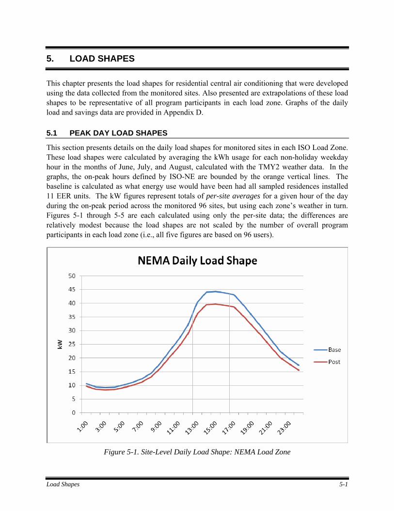
Load Shapes 5-1
5. LOAD SHAPES
This chapter presents the load shapes for residential central air conditioning that were developed using the data collected from the monitored sites. Also presented are extrapolations of these load shapes to be representative of all program participants in each load zone. Graphs of the daily load and savings data are provided in Appendix D.
5.1 PEAK DAY LOAD SHAPES
This section presents details on the daily load shapes for monitored sites in each ISO Load Zone. These load shapes were calculated by averaging the kWh usage for each non-holiday weekday hour in the months of June, July, and August, calculated with the TMY2 weather data. In the graphs, the on-peak hours defined by ISO-NE are bounded by the orange vertical lines. The baseline is calculated as what energy use would have been had all sampled residences installed 11 EER units. The kW figures represent totals of per-site averages for a given hour of the day during the on-peak period across the monitored 96 sites, but using each zone’s weather in turn. Figures 5-1 through 5-5 are each calculated using only the per-site data; the differences are relatively modest because the load shapes are not scaled by the number of overall program participants in each load zone (i.e., all five figures are based on 96 users).
Figure 5-1. Site-Level Daily Load Shape: NEMA Load Zone
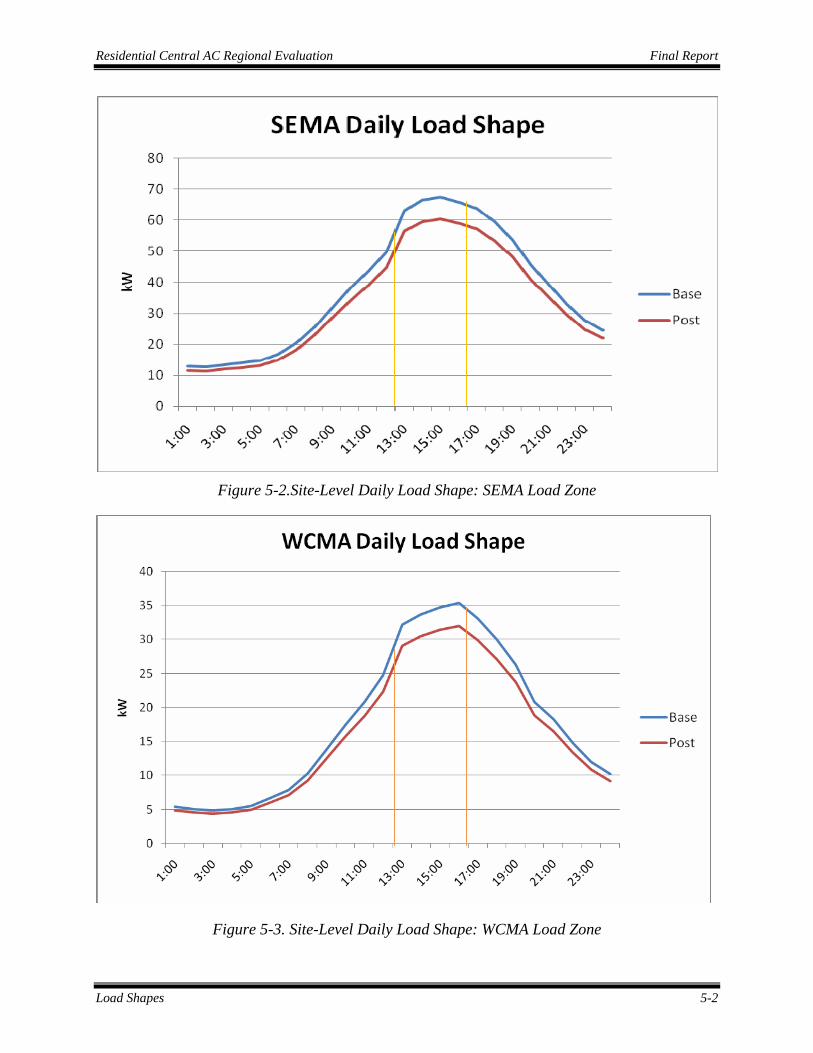
Residential Central AC Regional Evaluation Final Report
Load Shapes 5-2
Figure 5-2.Site-Level Daily Load Shape: SEMA Load Zone
Figure 5-3. Site-Level Daily Load Shape: WCMA Load Zone

Residential Central AC Regional Evaluation Final Report
Load Shapes 5-3
Figure 5-4. Site-Level Daily Load Shape: RI Load Zone
Figure 5-5. Site-Level Daily Load Shape: CT Load Zone

Residential Central AC Regional Evaluation Final Report
Load Shapes 5-4
Of the five load zones, SEMA has its heaviest use hours most closely aligned with the ISO-defined on-peak hours. Peak loads for other load zones come slightly later, with high points occurring around 6:00 PM. This difference is most notable in the CT load zone. This would be consistent with a residential occupancy pattern of residents largely absent from home during on-peak hours and turning on their AC after returning home from work.
5.2 DAILY SAVINGS LOAD SHAPES BY ISO LOAD ZONE
This section presents details on the hourly distribution of savings for each ISO load zone. The on-peak hours between 1 PM and 5 PM and is identified in each figure by orange bracketing. As with the annual savings load shapes, the figures chart out the difference between the baseline and post kW use figures from the previous section.
Figure 5-6. Daily Savings Load Shape: NEMA

Residential Central AC Regional Evaluation Final Report
Load Shapes 5-5
Figure 5-7. Daily Savings Load Shape: SEMA
Figure 5-8. Daily Savings Load Shape: WCMA

Residential Central AC Regional Evaluation Final Report
Load Shapes 5-6
Figure 5-9. Daily Savings Load Shape: RI
Figure 5-10. Daily Savings Load Shape: CT

Residential Central AC Regional Evaluation Final Report
Load Shapes 5-7
5.3 PEAK MONTH KW LOADS
This section presents monthly profiles for June, July, and August. Figure 5-11 shows the average CAC kW summed across sites during on-peak hours for both the monitored sites and the full participant population. Each trio of bars represents all 96 sites with the TMY weather for the given Load Zone used to calculate kW from the Tobit models.
Figure 5-11. Total On-Peak kW for Sampled Sites
In Figure 5-11 above, the kW values are the sum of the predictions during on-peak hours across all 96 sampled sites, i.e., the whole sample is applied to each column. Figure 5-12 below contains the average on-peak kW by month for the whole participant population. As such, the values are skewed by the overall program size by load zone, with the CT Load Zone displaying disproportionately large on-peak loads due to much higher program participation.

Residential Central AC Regional Evaluation Final Report
Load Shapes 5-8
Figure 5-12. Total On-Peak kW for Participant Populations

Summary and Conclusions 6-1
6. SUMMARY AND CONCLUSIONS
Estimates from the Tobit modeling developed and applied in this study were shown to have greater accuracy in predicting energy use than estimates developed through OLS regression, because monitoring of the sample houses showed that there are high proportions of zero energy use hours. The Tobit modeling methodology was especially useful for a geographic region such as New England, in which there are a significant number of residences with low cooling demands. By using the Tobit modeling, prediction accuracy (roughly, R2) was improved from 36% to 45%.
The results from using the Tobit models to predict kWh usage and savings show that higher efficiency CAC systems provide a sizeable reduction in annual kWh usage. These results, which are based on using TMY weather data, are summarized in Table 6-1.
Table 6-1. Summary of kWh Savings Estimates by ISO Load Zone (Based on TMY Weather Data)
ISO Load Zone Annual kWh Annual kWh Savings
NEMA 542,419 59,972 SEMA 164,158 17,996 WCMA 113,484 12,562
RI 166,178 18,425 CT 3,379,210 368,531
Using the Tobit models, predictions were also developed of kW reductions that result during seasonal peak hours from using high efficiency central air conditioning units. The kW reduction results, which are based on using actual 2008 weather data, are summarized in Table 6-2.
Table 6-2. Summary of Zone-Level Seasonal Peak kW Reductions (Based on Actual 2008 Weather Data)
Load Zone Average Seasonal Peak kW
Average Seasonal Peak kW Savings
9-Hour Total Seasonal Peak kW
9-Hour Total Seasonal Peak kW Savings
NEMA 633 69.9 5,697 630 SEMA 328.0 36.2 2,952 326 WCMA 343.7 38.3 3,094 344.9
RI 416.4 46.9 3747 424.4 CT 5,588.3 623.4 50,295 5,610
With the monitored data, On-Peak and Seasonal Peak coincidence factors were calculated for each load zone. They are detailed in Table 6-3 below.

Residential Central AC Regional Evaluation Final Report
Summary and Conclusions 6-2
Table 6-3 On-Peak and Seasonal Peak Coincidence Factors (Based on Actual 2008 Weather Data)
Load Zone On-Peak
Coincidence Factor
Seasonal Peak
Coincidence Factor
NEMA 43% 46% SEMA 42% 76% WCMA 28% 73%
RI 36% 80% CT 44% 72%
There are several methods by which the New England Utilities could increase the cost-effectiveness of future residential CAC programs in terms of kWh per ton saved.
• Our sample only had 6 units that were over 13 EER, and a total of 25 that were over 12. The New England Utilities could raise the EER (or SEER) standard required for participation in the program, though it is possible that this could lower the number of program participants as it would increase the average cost of a qualifying CAC system.
• Another possibility is to provide extra incentive for units that have two-stage operation. This allows the units to run at a reduced load when full cooling is not needed. This would not provide extra savings during the seasonal peaks, as in such cases anyone that is running their CAC at home would require the full cooling load, unless their CAC is oversized. However, during peak hours (non-holiday weekdays in June – August from 1-5 PM), many units could operate in their lower stage, increasing peak kW reduction to a significant degree (and more cost effectively than purchasing higher EER). However, such units are well represented in the sample, with 24 out of 96 CACs having two-stage operation, so an extra incentive for this feature would have some degree of built-in free-ridership.
The other primary area where program cost effectiveness could be improved upon is in participant selection.
• There were participants that were very low-volume, and in many cases these users were installing their first CAC, having relied upon windows and fans for cooling prior to this program. These participants are likely used to responding to high temperatures without CAC and to some degree continue to respond as such even with CAC available. Without prior data of the participant’s CAC use, this is one of few indicators available to screen participants.
• A second such indicator is CAC size. On average, we found that CAC usage was heavier for the smallest and largest ends of the distribution (units less than 2 tons or 4 tons or greater). Across all load zones, 1.5 ton units averaged 516 equivalent full load hours, with values of 485 and 729 for 4 and 5 ton units, respectively. Granted, these unit sizes did not have a statistically significant sample size, but it is an avenue that warrants further explanation. For 1.5 ton units, it is possible that they need to run more often on account of being undersized

Residential Central AC Regional Evaluation Final Report
Summary and Conclusions 6-3
for the residence. For larger units, they are presumably installed in larger homes, and as such the resident may be more accustomed to CAC usage. In addition, larger units may be oversized, and if so would overcool the residence when they are used for humidity control, if the CAC does not have two-stage operation.

Appendix A A-1
APPENDIX A. DATA COLLECTION FORMS
This appendix contains copies of the forms used for data collection.

Residential Central AC Regional Evaluation Final Report
Appendix A A-2
Air Conditioning Residential Duct Leakage Measurement Form Date: __________ Customer Name: ID #: ___________
Address: City: ______________________
Measurement team crew members: _______________________________ _________________
# of A/C units: # of Floors: # of Returns: _____________
House Conditioned Floor Area in Sq.Ft:
Windows Panes: 1 2 3
Attic Insulation: R-_____, Type ___________________, Inches __________
A/C Unit Condenser Location: _____________________________________________________
Air Handler location (attic, crawl space, garage, closet, other) ____________________________
Thermostat: Programmable ____ Manual ____ Cooling Temperature Setpoint:_________ºF
Type of unit: A/C only Heat Pump A/C w/ elec. heat A/C w/ gas heat
Unit Name Plate Data: Readable Not Readable
Make_________________________________ Model ______________________________
Compressor: Volts Amps Hp:
Outdoor Fan: Volts Amps Hp:
Sensible Capacity (kBTU/hr): Latent Capacity (kBTU/hr): _______________
Tons: COP or EER or SEER:
Old AC Unit Information: Age ________________ Tons _________
Other Notes: ___________________________________________________________________
______________________________________________________________________________
Data Logger: Motor On/Off logger Serial Number: _______________________________________________
Indoor Temperature logger Serial Number: ___________________________________________
Logger locations: _______________________________________________________________
Install Date: _________ Removal Date:

Residential Central AC Regional Evaluation Final Report
Appendix A A-3
Date: Time:
Duct Leakage to Unconditioned Space
Conditions Volts ac Amps kW Power factor
Outdoor Unit Power Air Handler Power Sum Total
Run Air Conditioning for at least 10 minutes then measure:
Return Air Temperature: ______ ºF
Supply Air Temperature: ______ ºF
Static Pressure, Pascals
(Supply Plenum with respect to Outside)
Airflow rate, cfm
Alternate Pressure
System Static Pressure, Pascals (supply plenum) System Fan On, cfm from Duct Blaster) for Total Airflow
Total Duct Leakage – at 25 Pascals (from Duct Blaster, House NOT pressurized) *
Duct Leakage to Unconditioned Space – at 25 Pa (from Duct Blaster, House pressurized) * **
Infiltration of Building & Ducts (Blower Door Only)
One-Time Electrical Measurements:
Other Notes:

Appendix B B-1
APPENDIX B. MODEL DEVELOPMENT
This appendix provides details of the methodology used for sample stratification, correcting for outliers, the SAS code for development of the Tobit models, and alternative models considered.
B.1 SAMPLE STRATIFICATION
For the sampling, sample points were allocated to give appropriate representation of units with different efficiencies (e.g., SEERs). Table B-1 shows the projected numbers of central air conditioning systems that Sponsors expected to rebate for different efficiency levels. As can be seen, it was expected that there would be representation for systems with different levels of efficiency.
Table B-1. Projected Number of CAC Systems to be Installed in 2008 under Sponsoring Utilities’ Programs
CAC Equipment Efficiency National
Grid (MA)
National Grid (RI)
NSTAR UI CL&P
AC SEER 14 (EER 11.5-11.99) 194 122 417 1,800 AC SEER > 14 and < 15 (EER ≥12) 129 18 205 AC SEER > 15.0 (EER ≥ 12.5) 73 10 409 450 Totals 396 150 1,031 2,250 1,000
The information in Table B-1 was used to prepare the allocation of sample points across utility service areas and equipment categories. Note that allocation by utility service area was used for two reasons. First, utility service area effectively serves to give proxy representation of different weather zones. Second, because records of customers participating in a program are kept by each utility, identification, selection, and recruitment of customers for the monitoring was facilitated.
A relatively balanced sampling plan was proposed to aid in estimation of the regression model for explaining air conditioning usage.
• First, the sampling plan provided for the widest ranges of values for the independent variables that are included in the regression model (i.e., equipment efficiency, weather conditions) that is possible, given the data that was available. Because the regression model will be estimated over the range of values representative across the region, the model will be less biased and more robust. Moreover, it can be used to analyze or project energy use for efficient central air conditioning equipment throughout the region.
• Second, the plan gave sufficient sample points to estimate reliably the coefficients for the independent variables. For example, there will be about 30 sample points for each efficiency level and 20 sample points for each utility area (except NGrid-RI).
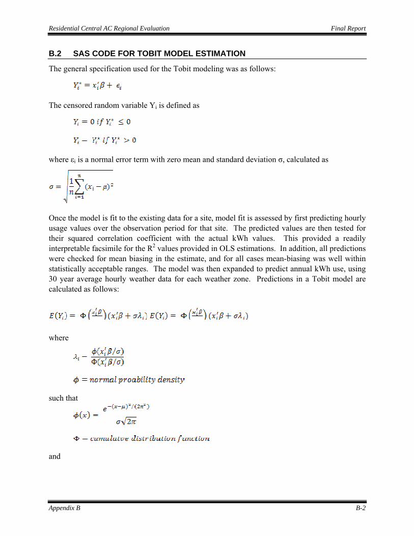
Residential Central AC Regional Evaluation Final Report
Appendix B B-2
B.2 SAS CODE FOR TOBIT MODEL ESTIMATION
The general specification used for the Tobit modeling was as follows:
The censored random variable Yi is defined as
where εi is a normal error term with zero mean and standard deviation σ, calculated as
Once the model is fit to the existing data for a site, model fit is assessed by first predicting hourly usage values over the observation period for that site. The predicted values are then tested for their squared correlation coefficient with the actual kWh values. This provided a readily interpretable facsimile for the R2 values provided in OLS estimations. In addition, all predictions were checked for mean biasing in the estimate, and for all cases mean-biasing was well within statistically acceptable ranges. The model was then expanded to predict annual kWh use, using 30 year average hourly weather data for each weather zone. Predictions in a Tobit model are calculated as follows:
where
such that
and

Residential Central AC Regional Evaluation Final Report
Appendix B B-3
This model creates maximum likelihood estimators (MLE), defined as follows:
.
Since maxima are unaffected by monotone transformations, one can take the logarithm of this expression to turn it into a sum:
The Tobit model, like all MLE’s, seeks to maximize , the probability of a given xi equaling a specific value.
Individual Tobit models were developed in SAS using the following code: proc lifereg data = hourly outest=OUTEST (keep=_scale_); /*Creates a temporary SAS Dataset from the model output, dropping all variables except the scale coefficient*/ model (lower,kwh_adj) = Weekend weekendtempdb weekendtempwb weekendEMATempdb weekendEMATempwb Temp_db Temp_wb EMA_temp_db EMA_temp_wb night nightTempdb nightTempwb nightEMATempdb nightEMATempwb afternoon afternoonTempdb afternoonTempwb afternoonEMATempdb afternoonEMATempwb / maxiter = 500 d=NORMAL; /*Sets the maximum number of iterations and identifies the distribution used as normal*/ title 'Tobit Estimation of KWH_ADJ Use'; output out=OUT xbeta=Xbeta; run;
The SAS lifereg procedure is a survival analysis model designed to predict the probabilities of events. With proper parameters set, this mimics the Tobit model, with the censored value (zero energy use) constituting an “event” with a certain probability of occurring, given temperature and time inputs. In the above code, the variable “lower” is defined as equaling kWh_adj where positive, and as having no value where kWh = 0. The code presented below was run to develop Tobit forecasts.

Residential Central AC Regional Evaluation Final Report
Appendix B B-4
data predict ; drop lambda _prob_ _scale_; set out; if _n_ = 1 then set outest; lambda = pdf('normal',Xbeta/_scale_)/cdf('normal',Xbeta/_Scale_); Forecast = cdf('normal',Xbeta/_scale_)*(Xbeta+_scale_*lambda); label Xbeta= 'Mean of Uncensored Variable' Forecast = 'Mean of Censored Variable'; run;
B.3 TOBIT MODELS COMPARED TO ALTERNATIVE MODEL SPECIFICATIONS
As part of the model development effort, the Tobit specification was compared against alternative specifications, including OLS regression models and a fixed effects model that provided site-specific dummy variables for each site. Based on comparison of R2 values, it was concluded that Tobit modeling was the best choice. Tobit modeling provided R2’s upwards of 12% greater than those obtained through fixed effect modeling.
B.3.1 Fixed Effects Modeling The fixed effects model is a method to account for unobserved heterogeneity, i.e., individual idiosyncrasies that cannot be quantified. This is relevant in modeling CAC use, as personal tastes and characteristics can significantly affect usage. For example, several monitored sites only displayed usage at night, likely due to no one being home during the day. In addition, even if a thermostat setpoint is maintained relatively consistently (which is itself a rare occurrence with residential CAC), this set point differs greatly from home to home, from day to day, and by hour in the case of programmable thermostats (which 85% of the sample had), with temperature ranges observed at the 96 samples sites as high as 82 and as low as 70.
With fixed effect modeling, each CAC unit would be assumed to have the same weather response coefficients once the dummies for individuals and time periods are accounted for. However, that may provide an inaccurate depiction of responses to weather changes, as the only site-specific factor it accommodates is the tipping point where the CAC unit begins running, averaging out differences in magnitude of reaction. This contrasts with what is observed in the monitored data, in that the responses to weather changes after the tipping point has been reached for individual units can vary widely.
Rather than trying to gather information on each of these characteristics to individually control for them at each site, the fixed effects model creates a series of zero-one dummy variables, one for each site and one for each time period. Essentially, this subtracts each individual’s mean value from each of their observations before estimating the model. In addition, with the addition of dummies for time parameters, anything unique to a given hour beyond its temperature is

Residential Central AC Regional Evaluation Final Report
Appendix B B-5
factored into its dummy variable and removed from parameter estimates for weather variables. This is calculated as follows:
where yit is the dependent variable observed for individual i at time t, β is the vector of coefficients, xit is a vector of regressors αi is the individual effect and uit is the error term. From this model, the estimator is
where
occurring for individual i at time t.
It should be noted that this model cannot directly estimate the coefficients of time-invariant variables; it aggregates them into a site- and time- specific mean and subtracts them from the data prior to model estimation. The results from this model had an R2 of 33%, less than the average R2 of both OLS and Tobit estimations.
This model postulates that site-specific idiosyncrasies can be corrected by changing just the intercept of an individual model. It argues that beyond changes of the intercept (essentially, changes of the “tipping point” where an individual begins running their CAC), responses to weather should be the same across individuals. We would assert that differences across individuals are greater than the fixed effects methodology can effectively model. The rationale for this assertion is that the collected data indicates that responses to weather do not just vary in when an individual begins using their CAC; they also vary in the magnitude of their response. Hence, the coefficients for each site for weather variables should differ. Modeling each site individually, and then weighting the forecasts of the results, accounts for site-specific idiosyncrasies in a way that does not place artificial limits on individual reaction functions to weather. By keeping site-level data disaggregated, site-specific idiosyncrasies are captured in the coefficients of the unit-specific models.
B.3.2 OLS Regression Modeling Modeling through Ordinary Least Squares (OLS) regression modeling was not considered to be an appropriate method for this study. One of the underlying assumptions for OLS modeling is that the error term for a given observation is uncorrelated to the independent variables for that same observation across the range of data. This assumption is violated in this study in that the data has two tiers:

Residential Central AC Regional Evaluation Final Report
Appendix B B-6
1. For a given site, below a certain temperature range, all kWh values equal zero. As a result, the variance for that temperature range equals zero as well.
2. Above this temperature range, when the data begins to display positive kW values, variance becomes > 0.
3. Therefore, the variance of OLS estimates is positively correlated with temperature.
In order to account for this, OLS modeling gives excessively high standard error values for each coefficient estimate, so the significance tests cannot be trusted. As such, OLS is not the minimum variance estimator for this data.
The Tobit estimation could correct for heteroskedasticity in this data, because it disaggregates the positive from the zero values. To verify this, the Breusch-Pagan test for heteroskedasticity was applied for two ranges of data on each site:
1. For all observations where kWh > 0
2. For all observations, including both zero and non-zero values.
Table B-2 reports the median values from the site-level heteroskedasticity test results. In this test, a high Chi-Square (and subsequently, a low p-value) means a rejection of the assumption of homoskedasticity, i.e., the data is heteroskedastic.
Table B-2. Breusch-Pagan Test Results
Positive Values All Values Degrees of Freedom 153 172 Chi-Square 136 258 Pr. > Chi-Square 0.77 0.0001
The test results indicate that for all positive values of kWh, the variance of estimates is not correlated with the independent variables. As a result, for that range of data, the estimates of standard errors are accurate. However, for the whole range of data. including both positive and zero values, the variance of estimates is correlated with the independent variables. The Tobit model accounts for this tiering of the data by re-forecasting the zero values to their “true” negative values. In doing so, it separates the zeros from the positive values and estimates standard errors for each tier individually, producing unbiased estimates of standard errors for coefficients in the model.
Another option was to run Ordinary Least Squares (OLS) regressions restricted to non-zero values for kWh. We opted for Tobit estimation, as opposed to running OLS only for the non-zero values for kW, because the Tobit estimation gives greater precision and reduced standard errors. This is the case because if the data set is truncated to include only positive values for energy use, the OLS model would be based on far fewer observations than used in the Tobit estimation. For example, the sample size would be reduced by more than 85% for some sites. The Tobit modeling procedure allows all observations to be incorporated into the model

Residential Central AC Regional Evaluation Final Report
Appendix B B-7
development in a manner that allows for an increased probability of zero energy use, without biasing estimates of positive energy use.
The accuracy of the Tobit modeling procedure was compared against the OLS and Fixed-Effect modeling, using R2 values as the measure of accuracy. A summary of this comparison is provided in Table B-3. The Tobit modeling was found to be more accurate for all Load Zones.
Table B-3. Forecast R2’s for Tobit Models versus OLS Models
Average R2 Median R2 Tobit .452 .448 OLS .362 .352 Fixed Effects .3321 -
Although the Tobit models were accurate estimators for most usage patterns, there were a small number of sites where usage patterns were not significantly weather-dependent. For such sites, a Tobit model could not accurately forecast their use outside of the cooling season. Examples include sites where over the monitoring period (ranging from July-September) the participant only ran their CAC unit at night. As a consequence, regression models predict that their AC usage has a negative relationship with temperature. For such sites, calculations outside of the months of May through September proved erratic, as there was not sufficient variation in temperature in the monitored data to pattern their behavior during winter temperatures.
B.3.3 Exponentially Weighted Moving Average Tobit Model Tobit models with lag weighting were compared to models with an exponentially weighted moving average. In this alternate model, the moving averages were calculated as
where
with n = the number of periods of the moving average. This weighting system imposes a structure by which the dry bulb temperature measurement’s effect on current energy use declines at an increasing rate as the lag length increases. This model displayed lower R2 than the lag weighting used in the final model, primarily because it imposed a structure that was not borne out in the data.
1 Fixed effects model aggregates all sites into one model rather than modeling each individually

Residential Central AC Regional Evaluation Final Report
Appendix B B-8
B.4 MODEL CHECKS USING INDOOR TEMPERATURE MEASUREMENTS
During the site visits, indoor temperature loggers were installed adjacent to each thermostat. The temperature data collected with these temperature loggers were used to check compressor motor logger data, particularly if the motor logger data for a site appeared erratic. The indoor temperature data collected were not used in development of the site-level regression models, as such data would not be available for the entire year for annual estimates.
Indoor temperature data was collected with Hobo Pro temperature loggers. The temperature loggers were placed adjacent to the CAC unit’s thermostat in a given residence. A second one was placed if the CAC unit was a dual-zone with two thermostats. Large homes served by either two separate units or two thermostats also had two indoor temperature loggers installed. At installation, the loggers were set to collect temperature data at 10 minute intervals.
The indoor temperature data were compiled into hourly averages and aggregated by regional weather station. The five stations used were:
• Boston, MA
• Worcester, MA
• New Haven, CT
• Hartford, CT
• Providence, RI
B.3.1 Average Indoor Temperature Figure B-1 shows daily averages of indoor temperature measurements, where the averaging is across monitored sites. It should be noted that due to difference in monitoring periods, some dates have fewer observations than others, particularly at the very beginning and end of the overall monitoring period. The month of August had the greatest representation in terms of sample points with indoor temperature monitoring. In the figure below, the blue line is average indoor temperature. The red and green lines are average outdoor dry and wet bulb temperature, respectively.

Residential Central AC Regional Evaluation Final Report
Appendix B B-9
Figure B-1. Average Indoor Temperature from Monitored Sites
B.3.2 On-Peak Indoor Temperature Averages This section presents summary statistics for monitored indoor temperature within the sample. The data is subdivided by month and by weather station. The data are summarized in terms of average temperatures for the months of July and August from the hours of 1-5 PM on non-holiday weekdays.
Table B-4. On-Peak Indoor Temperatures, July 2008
Weather Station Mean Standard Deviation Minimum Maximum
Boston, MA 75.7 1.306 70.8 77.2 Worcester, MA 75.1 0.664 73.9 76.7 New Haven, CT 75.9 0.531 74.5 77.1 Hartford, CT 76.5 6.037 70.7 91.7 Providence, RI 77.3 0.734 75.3 79.3

Residential Central AC Regional Evaluation Final Report
Appendix B B-10
Table B-5. On-Peak Indoor Temperatures, August 2008
Weather Station Mean Standard Deviation
Minimum Maximum
Boston, MA 74.8 0.902 72.5 76.7 Worcester, MA 74.9 1.167 71.8 76.9 New Haven, CT 75.7 0.910 73.0 77.1 Hartford, CT 72.7 0.537 71.2 74.1 Providence, RI 76.4 1.036 73.7 78.7
Hartford shows more extremes in indoor temperature than other cities. This can largely be attributed to several anomalous sites, as the mean value is not that far deviated from the other cities examined.
B.5 TESTING FOR OUTLIERS
To gauge the variation in predictions from the Tobit models across sites, summary statistics were calculated for three output variables from the site-specific Tobit models: average hourly kW during the monitoring period, average on-peak kW reduction from the predicted data, and average on-peak kW reduction per ton from the predicted data. The calculated means and standard deviations are reported in Table B-6. For these categories, the summary statistics have been calculated both with and without outlier values.
Table B-6. Summary Statistics for Variations of Tobit Model Results across Sites
Variable Mean Standard Deviation
Coefficient of Variation
Full Data Set Average hourly kW during monitoring period
.21 .22 1.07
Average on-peak kW reductions .059 .058 0.98 Average on-peak kW reductions per ton
.022 .018 .84
Outliers Not Included Average hourly kW during monitoring period
.16 0.12 .76
Average on-peak kW reductions .049 0.037 .77 Average on-peak kW reductions per ton
.022 .016 .733
The coefficients of variation thus calculated are higher than anticipated during the sample development for this study. However, there is likely a result because of outliers in the sample. To test for this, Grubb’s Test was used to identify observations that were outliers. The Grubb’s test defines a critical value above which an observation is considered an outlier, as a function of

Residential Central AC Regional Evaluation Final Report
Appendix B B-11
the sample size and t-distribution critical value, for a given significance level and degrees of freedom.
The Tobit models used were approximated with a normal distribution, as this provided the best log-likelihood scores, so the Grubb’s test is applicable. The G-statistic is defined as follows.
• For tests of upper outliers and
• For tests of lower outliers.
The value from these equations has to exceed the critical value, G*. The critical value is calculated as follows:
= Upper critical value of the t distribution with N-2 degrees of freedom and a significance level of ά/2N.
For this study, the test is a two-tailed test at the 10% level of precision with 94 degrees of freedom. As such, the upper critical value of the t-distribution is 1.66. It is important to note that this test cannot be run in multiple iterations. The first time the test is run, it checks for outliers of a random sample. If multiple iterations of the test are run, then values that originally were not considered outliers in the random sample can become outliers in the new reduced sample.
When this test was run on the observed hourly kW averages, 7 upper outliers and no lower outliers were identified. The outliers are identified in Table B-7:

Residential Central AC Regional Evaluation Final Report
Appendix B B-12
Table B-7. Outliers and G-Statistics, Monitored Data
Average Monitored Hourly kW G-Statistic
1.41 5.31 0.56 1.55 0.54 1.44 0.56 1.53 1.22 4.48 0.56 1.54 0.81 2.63
G-Critical Value: 1.28 Sample Mean: .21
Standard Deviation .22
The same test was run on average on-peak kW reduction for each load zone. The results of the Grubb’s test are presented in the tables below for each ISO Load Zone.
Table B-8. Outliers and G-Statistics: NEMA
Average On-Peak kW Reduction G-Statistic
0.31 1.76 0.29 1.68
G-Critical Value: 1.28 Sample Mean: .047
Standard Deviation .053
Table B-9. Outliers and G-Statistics: SEMA
Average On-Peak kW Reduction G-Statistic
0.17 1.34 0.24 1.69 0.18 1.38 0.39 2.16 0.35 2.07 0.23 1.65 0.16 1.39
G-Critical Value: 1.28 Sample Mean: .071
Standard Deviation .066

Residential Central AC Regional Evaluation Final Report
Appendix B B-13
Table B-10. Outliers and G-Statistics: WCMA
Average On-Peak kW Reduction G-Statistic
0.23 1.51 0.38 2.01 0.35 1.90 0.20 1.36
G-Critical Value: 1.28 Sample Mean: .061
Standard Deviation .064
Table B-11. Outliers and G-Statistics: CT
Average On-Peak kW
Reduction G‐Statistic
0.22 1.89 0.13 1.39 0.16 1.59 0.15 1.51 0.13 1.35 0.13 1.36 0.13 1.34 0.23 1.94 .13 1.35
G‐Critical Value: 1.28 Sample Mean: .055
Standard Deviation .045
Table B-12. Outliers and G-Statistics: RI
Average On-Peak kW Reduction G-Statistic
0.23 1.58 0.38 2.07 0.35 1.97
G-Critical Value: 1.28 Sample Mean: .061
Standard Deviation .062
There is an additional step required when applying the Grubb’s test to on-peak kW demand reduction, however, in that the values for this parameter are not normally distributed. To correct for this, Grubb’s test was run against the natural log transformations of average on-peak kW reduction. Following this transformation, the Grubb’s Outlier Test indicated 7 upper outliers and

Residential Central AC Regional Evaluation Final Report
Appendix B B-14
no lower outliers for the average hourly kW from the monitored data. The summary statistics for average hourly kW demand during the monitoring period with outliers removed is reported in Table B-6 above.
Grubb’s Outlier Test was then run on the average on-peak kW demand reduction for each load zone. Since each load zone has its own 96 observations, the outliers removed in this calculation of c.v are removed from a total sample of 480. It is important to note, however, that no outliers were removed when calculating kWh and kW savings; outliers were removed only in calculations of the c.v.’s. For the predicted data, the distribution of upper outliers by load zone was as follows:
Table B-13. Number of Outliers by Load Zone
NEMA WCMA SEMA RI CT Sample Points 2 4 7 3 9
There were no lower outliers in any of the load zones. The summary statistics following removal of the outliers for this parameter are also reported in Table B-6.
There are a number of reasons to account for the variations across sample sites. First, there were a significant number of program participants that were installing a CAC unit at their home for the first time. As such, usage for these homes could not be determined a priori during sample development. This resulted in an error in stratification during sampling, as program participants were stratified by service territory (as a proxy for load zone) and prior use. Without any prior use to compare against, there was no certain way to determine the proper strata for first-time CAC users. However, given the significant portion of the program participant database that this class of users consists of, it would have been inappropriate to exclude them. The findings showed that individuals that installed their first CAC as part of this program were among the infrequent users. Such users are likely accustomed to alternate methods of comfort during the peak cooling season (e.g., using fans, opening windows, etc.).
B.6 BREUSCH-PAGAN TEST FOR HETEROSKEDASTICITY
The Breusch-Pagan test for heteroskedasticity determines whether the error term from a regression is correlated with the model’s independent variables; in other words, for this model, heteroskedasticity implies that as temperature increases, the absolute value of residuals (errors) increases. Given a regression with error term u, the Breusch-Pagan test runs the following regression:
where Beta is a vector of independent variables in the model. Following this, all independent variables in the test regression are tested for joint significance against the squared error term. The test of joint significance is an F test defined as:

Residential Central AC Regional Evaluation Final Report
Appendix B B-15
where RSS1 is the residual sum of squares of the restricted model, RSS2 is the residual sum of squares of the unrestricted model, n is the sample size, p1 is the number of independent variables in the restricted model, and p2 is the number of independent variables in the restricted model. If the F statistic displays significance at the assigned rigor level (10% in this study), then we reject the null hypothesis of homoskedasticity, and the data is thus treated as heteroskedastic.

Appendix C C-1
APPENDIX C. INPUT AND OUTPUT DATA FOR MODELING EFFORT
This appendix discusses the input and output data for the site-specific modeling effort.
C.1 SUMMARY OF MONITORED AND PREDICTED DATA
A summary of monitored and predicted data is presented in Table C-1. These data are also included in the following file:
NE Res CAC Summary.xls
C.2 WEATHER DATA
The file below contains the local 2008 weather data used in the model development for monitored sites.
NE Hourly Weather.xls
C.3 TOBIT MODEL RESULTS: TEMPERATURE-ADJUSTED KWH VALUES
The file below contains the results from the Tobit modeling for all sites using temperature-adjusted kWh values. It is presented in the following manner: 1. Variable coefficient 2. Variable Chi-Square (values in parentheses)
Site Level Regression Summaries.xls
Note that the Scale variable is a site-specific constant that has no chi-square or P-value.
C.4 TEMPERATURE THRESHOLDS FOR SECOND-STAGE USE
Table C-2 below presents the thresholds for second-stage use at each discrete unit size. These values were derived by calculating the average cooling load at various outdoor temperatures in New England, and using the average figure where first-stage cooling provides 68% of the full CAC capacity. The figures in Table C-2 can be interpreted as follows: on average, for a 3-ton, two stage CAC the cooling load will be in the first stage for dry bulb temperatures under 81 deg. F. These cutoffs were calculated incorporating New England weather data in residential simulations. As such, it can be concluded that two-stage units will remain in the first stage for most humidity-based CAC demand.

Residential Central AC Regional Evaluation Final Report
Appendix C C-2
Table C-1. Summary of Monitored and Predicted Data for Monitored CAC Units
Site ID Utility Load
Zone EER Tons 2 stage
Spot kW @ °F Max
kWDays Monit
µ °F indoor
min out °F if On
% time On
% hrs On
AC kWh Monitored
AC ann kWh
kWh saved
% ∆ kWh
House CF
Infil cf/min
Infil ACH
39 CL&P CT 11.1 3.5 - 3.120 84.9 2.87 48.67 72 57.0 11% 32% 353 1006 5 0%20 NSTAR NEMA 11.5 4 X 3.384 73.0 2.38 54.71 74 61.0 1% 4% 30 32 1 5% 21,250 131 .5814 NGrid-MA WCMA 11.5 3 - 2.151 75.0 2.22 39.67 . 62.1 7% 23% 154 383 17 4% 15,725 86 .5028 CL&P CT 11.5 2.5 - 1.740 81.0 0.00 47.50 73 63.0 0% 0% 0 0 0 - 13,872 78 .2788 NGrid-MA WCMA 11.5 2.5 - 1.772 64.9 2.08 38.04 74 57.0 11% 25% 195 612 28 5% 13,600 178 .4951 NSTAR NEMA 11.6 2.5 X 1.787 64.0 1.73 38.00 77 59.0 10% 41% 135 791 43 5% 6,970 58 .9478 NSTAR NEMA 11.7 2 - 1.511 75.9 1.45 38.92 75 62.1 3% 8% 35 317 19 6% 25,500 302 .9254 NSTAR NEMA 11.7 2 - 0.759 75.0 0.79 53.08 75 60.1 8% 16% 72 229 15 6% 21,250 154 .5155 NSTAR NEMA 11.7 3 - 2.065 75.0 2.19 53.00 74 55.9 10% 35% 259 834 53 6% 21,250 16445 NGrid-MA SEMA 11.7 2.5 - 2.484 87.1 2.96 48.96 76 62.1 2% 4% 73 229 15 7% 15,955 295 .4259 NGrid-MA NEMA 11.7 2.5 - 2.071 72.0 0.01 64.96 71 66.9 0% 0% 0 0 0 - 10,200 .6146 NGrid-MA WCMA 11.7 3 - 1.349 72.0 1.53 44.00 . 53.1 22% 64% 336 844 54 6% 17,850 23 .4086 NGrid-MA SEMA 11.7 2 - 1.670 70.0 1.94 41.25 74 63.0 9% 21% 159 866 55 6% 10,200 808 .924 NGrid-RI RI 11.8 3 - 1.289 73.9 1.46 41.00 . 59.0 13% 29% 191 862 521 60% 24,990 26 NSTAR NEMA 11.8 2 - 1.683 71.1 2.36 45.92 74 64.0 3% 7% 76 249 18 7% 21,250 114 .7676 NGrid-MA WCMA 11.8 5 X 4.480 64.0 5.25 38.71 . 63.0 6% 13% 256 1848 134 7% 25,500 620 .4235 NSTAR NEMA 11.8 4 X 1.615 68.0 1.86 65.96 73 55.0 20% 45% 519 1318 96 7% 22,041 123 .7058 NSTAR NEMA 11.8 3 - 2.227 71.1 2.72 40.92 75 63.0 12% 42% 303 750 55 7% 25,500 .4783 NGrid-MA NEMA 11.8 3 - 2.577 70.0 1.71 33.67 75 69.1 1% 5% 24 237 17 7% 12,954 211 .8487 NGrid-MA NEMA 11.8 3 - 2.242 71.1 5.83 50.92 . 63.0 13% 18% 380 1652 120 7% 16,150 .5618 NSTAR NEMA 11.9 3 X 2.223 70.0 39.59 41.00 75 68.0 5% 11% 1388 1229 101 8% 13,600 .5324 NSTAR NEMA 11.9 4 - 3.173 84.0 2.63 57.83 73 59.0 11% 40% 479 1459 119 8% 22,525 122 .4271 NSTAR NEMA 11.9 3 X 1.910 82.0 1.97 58.96 71 57.9 13% 32% 308 806 66 8% 16,575 8 NGrid-MA NEMA 12 4 - 2.840 70.0 3.29 36.75 . 60.1 16% 36% 431 2171 197 9% 29,682 247 .8049 NSTAR SEMA 12 3 - 2.607 77.0 2.79 66.38 74 59.0 9% 32% 375 973 88 9% 29,793 388 .4410 NGrid-MA NEMA 12 3 - 3.748 79.0 1.81 34.71 76 64.0 3% 14% 80 261 24 9% 42,500 62 NGrid-MA WCMA 12 2.5 - 2.017 70.0 2.16 30.79 . 71.1 3% 11% 53 121 11 9% 21,250 146 .9663 NGrid-MA WCMA 12 2 - 0.529 70.0 0.25 30.71 . 69.1 1% 6% 5 29 3 10% 21,250 126 .9640 UI CT 12 2.5 - 2.065 79.0 2.23 61.46 . 60.1 24% 55% 715 1123 102 9% 11,050 331 1.5716 CL&P CT 12 3 - 2.050 77.0 1.86 38.92 75 57.0 17% 68% 263 1146 104 9% 16,728 97 .4125 NSTAR NEMA 12 2.5 - 2.106 71.1 1.88 47.88 75 64.0 6% 21% 128 196 18 9% 21,250 122 .7630 UI CT 12 3 - 2.130 79.0 2.08 49.67 77 55.9 30% 70% 548 2270 206 9% 22,100 .2131 NGrid-RI RI 12 2.5 - 1.610 64.9 1.97 48.21 76 59.0 13% 25% 267 1171 903 77% 8,500 1.3957 UI CT 12 2 - 1.993 84.9 1.67 28.96 75 72.0 17% 47% 228 843 77 9% 8,500 51 .6269 UI CT 12 3 X 2.591 86.0 2.51 46.96 78 63.0 24% 38% 626 1081 98 9% 20,400 340 .8448 NSTAR NEMA 12 2 - 1.758 80.1 1.90 51.00 73 64.0 12% 17% 246 529 48 9% 9,350 1.2141 CL&P CT 12 2 X 1.770 80.1 0.13 50.96 76 55.9 0% 0% 1 605 55 9% 14,450 127 1.0742 CL&P CT 12 2 - 1.868 73.0 1.67 27.96 74 60.1 12% 40% 154 59 5 9% 17,094 83 .5543 CL&P CT 12 1.5 - 1.170 76.0 1.32 43.75 71 60.1 22% 42% 271 868 79 9% 17,094 69 .5547 CL&P CT 12 3 X 2.280 69.1 2.41 39.13 77 63.0 10% 31% 236 1351 154 11% 16,745 645 .5575 CL&P CT 12 2 X 1.750 84.0 1.45 49.58 74 63.0 5% 19% 92 470 43 9% 10,625 63 .4568 NSTAR NEMA 12 3 - 2.264 69.1 2.38 55.00 73 61.0 6% 16% 180 661 60 9% 17,850 254 .6360 NGrid-MA WCMA 12 1.5 - 1.094 73.9 1.00 35.42 75 72.0 0% 1% 2 65 6 9% 14,450 172 .4285 NGrid-RI RI 12 2 X 1.305 64.9 1.55 39.38 78 64.9 1% 3% 19 215 48 22% 17,000 297 .5934 NSTAR NEMA 12 2.5 - 2.108 73.9 2.01 55.38 74 59.0 8% 37% 214 446 41 9% 9,350 108 .3890 UI CT 12 3 - 2.110 75.0 1.50 58.96 75 70.0 1% 4% 20 179 16 9% 27,200 553 .3991 UI CT 12 3 - 1.980 75.0 0.97 45.88 77 62.1 4% 33% 100 324 29 9% 11,900 149 1.5222 UI CT 12 2.5 - 2.243 80.1 1.59 54.75 70 54.0 9% 50% 255 634 58 9% 10,200 1,630 .687 NGrid-MA WCMA 12.1 2 - 1.859 70.0 1.99 41.71 . 64.0 4% 5% 70 345 35 10% 24,225 256 .759 NGrid-MA NEMA 12.1 4 - 3.112 79.0 2.56 54.96 72 63.0 2% 7% 76 131 13 10% 42,500 101 .2627 NGrid-RI RI 12.1 3 - 2.190 64.9 2.62 49.38 72 61.0 8% 31% 239 731 834 114% 14,688 64 .7484 NSTAR NEMA 12.1 3.5 - 3.220 73.0 3.48 47.29 75 57.9 5% 15% 186 704 70 10% 17,850 315 .9829 NSTAR NEMA 12.2 3 - 2.679 81.0 2.68 48.08 74 57.9 11% 32% 303 675 71 10% 16,941 163 .7015 CL&P CT 12.3 2 - 1.080 82.9 1.14 48.96 . 53.1 40% 81% 473 1296 147 11% 12,325 279 1.0144 NGrid-RI RI 12.3 3 - 2.640 81.0 2.59 54.96 75 59.0 10% 25% 315 1180 1261 107% 21,667 93 UI CT 12.3 3 - 2.504 84.9 2.38 59.88 74 66.9 4% 12% 123 280 32 11% 20,400 325 .795 CL&P CT 12.4 2 - 1.590 75.9 1.66 38.67 74 60.1 21% 56% 247 782 100 13% 20,740 67 .4932 NSTAR NEMA 12.4 3 - 2.440 78.1 2.58 48.71 76 68.0 3% 5% 85 272 35 13% 20,400 107 .1277 NSTAR NEMA 12.4 3.5 - 2.977 75.9 3.10 36.88 75 68.0 3% 5% 91 943 120 13% 25,500 277 .9264 CL&P CT 12.4 3 X 2.420 82.9 2.50 28.96 72 63.0 20% 38% 324 1094 139 13% 21,913 92 NGrid-MA NEMA 12.4 3 - 2.330 72.0 2.29 49.96 . 53.1 7% 28% 178 625 80 13% 17,026 .5594 NGrid-RI RI 12.5 3 - 2.160 82.0 2.25 42.00 76 61.0 13% 28% 259 1021 730 71% 15,504 103 .7689 UI CT 12.5 3 X 2.572 87.1 2.67 58.83 76 64.0 14% 31% 472 #N/A #N/A #N/A 27,200 12 NGrid-MA NEMA 12.5 3 - 2.586 75.0 2.26 46.96 72 63.0 3% 15% 95 335 46 14% 33,473 61 NGrid-MA WCMA 12.5 2 - 1.454 68.0 1.53 29.96 75 61.0 6% 15% 62 383 52 14% 10,200 1,032 .7752 CL&P CT 12.5 2 - 1.640 86.0 1.65 38.54 70 63.0 1% 4% 20 291 40 14% 16,873 53 NSTAR SEMA 12.5 3.5 - 3.073 84.0 2.95 50.92 77 62.1 13% 42% 459 1300 177 14% 17,000 221 .7280 UI CT 12.5 2 - 3.272 81.0 3.50 56.96 74 68.0 4% 9% 170 536 73 14% 17,000 82 .92
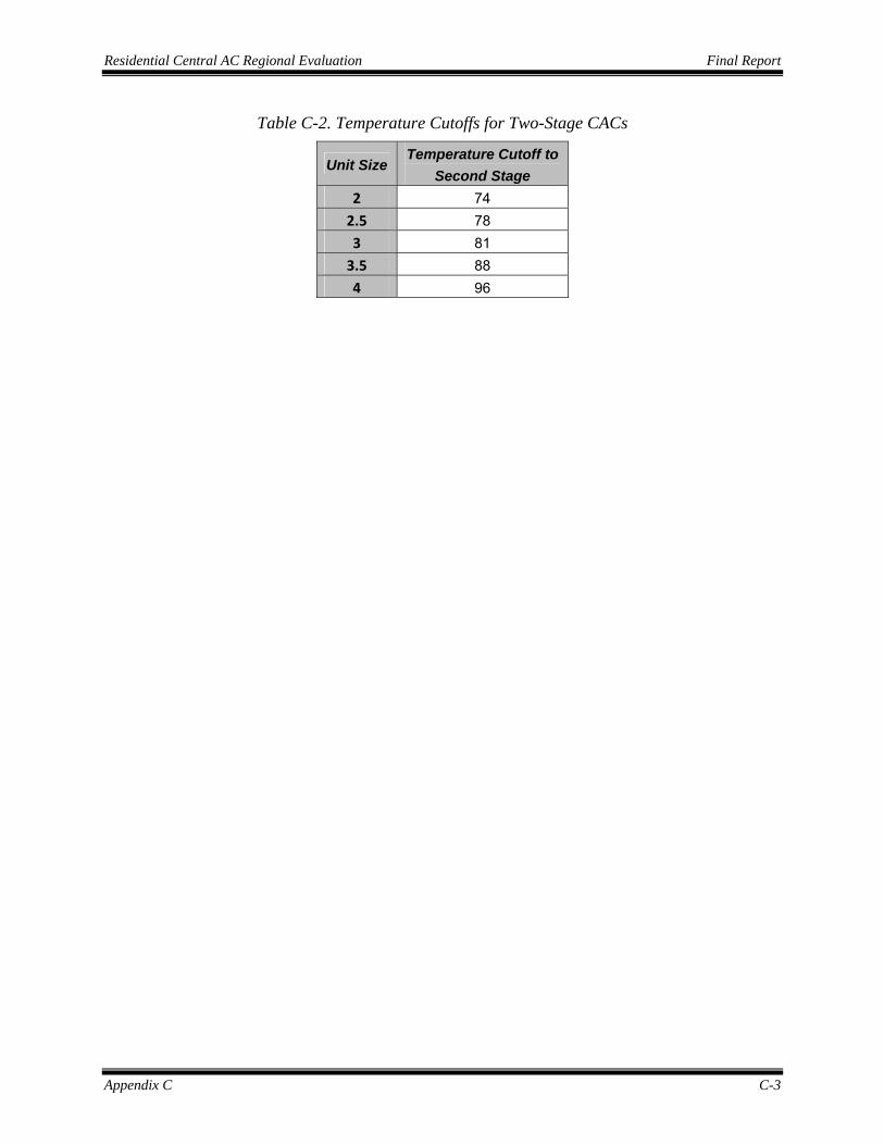
Residential Central AC Regional Evaluation Final Report
Appendix C C-3
Table C-2. Temperature Cutoffs for Two-Stage CACs
Unit Size Temperature Cutoff to
Second Stage 2 74 2.5 78 3 81 3.5 88 4 96

Appendix D D-1
APPENDIX D. GRAPHICAL REPRESENTATION OF LOAD DATA
This appendix provides graphs showing the annual load and savings data for the various ISO load zones.
D.1 ANNUAL LOAD DATA BY LOAD ZONE
This section provides graphs of load data for all program participants in each ISO Load Zone. When examining the graphs of zone-level load shapes it is important to take into account the number of total program participants in each load zone. For example; the CT load zone had over 3,200 participants, several times as many as other load zones (with the lowest being SEMA with 196).
Figure D-1. Baseline and Post Installation Annual Load Shapes: NEMA

Residential Central AC Regional Evaluation Final Report
Appendix D D-2
Figure D-2. Baseline and Post Installation Annual Load Shapes: SEMA
Figure D-3. Baseline and Post Installation Annual Load Shapes: WCMA
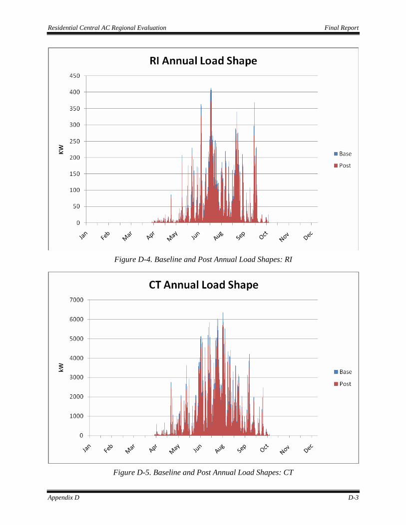
Residential Central AC Regional Evaluation Final Report
Appendix D D-3
Figure D-4. Baseline and Post Annual Load Shapes: RI
Figure D-5. Baseline and Post Annual Load Shapes: CT

Residential Central AC Regional Evaluation Final Report
Appendix D D-4
D.2 ANNUAL SAVINGS LOAD DATA
This section provides savings load data for program participants in each load zone. The baseline used for the calculation of savings load shapes is defined as what kWh use would have been had all program participants installed 11 EER units. The figures in each of these graphs are measured in hourly kWh and are the difference between the baseline and post graphs from Section 5.1. As with the graphs from the previous section, the figures presented in this section are a function of the quantity of units. As such, load zones with a larger number of participants show higher savings totals.
Figure D-6. Annual Savings Load Shape: NEMA
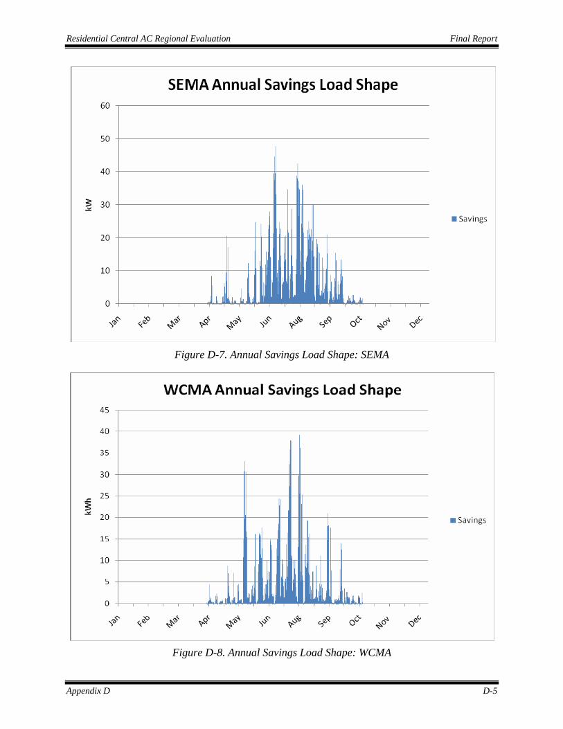
Residential Central AC Regional Evaluation Final Report
Appendix D D-5
Figure D-7. Annual Savings Load Shape: SEMA
Figure D-8. Annual Savings Load Shape: WCMA

Residential Central AC Regional Evaluation Final Report
Appendix D D-6
Figure D-9. Annual Savings Load Shape: RI
Figure D-10. Annual Savings Load shape: CT

Appendix E E-1
APPENDIX E. SAVINGS TABLES
This appendix contains tables showing the underlying savings by unit size class that were used to estimate aggregate savings by load zone.
E.1 SITE-LEVEL ANNUAL SAVINGS BY UNIT SIZE (TMY WEATHER DATA)
Table E-1. Average Site-Level Savings: NEMA Load Zone Weather
Unit Size (Tons)
Number of Units
Average Annual kWh
Annual kWh Savings
Annual kWh Savings
Per Ton
Equivalent Full Load Operating
Hours 1.5 2 545 50 33 477 2 26 367 43 21 251
2.5 18 425 48 19 227 3 38 724 88 29 334
3.5 4 786 81 23 255 4 7 1278 136 34 454 5 1 2520 183 37 562
Table E-2. Average Site-Level Savings: SEMA Load Zone Weather
Unit Size (Tons)
Number of Units
Average Annual kWh
Annual kWh Savings
Annual kWh Savings
Per Ton
Equivalent Full Load Operating
Hours 1.5 2 587 53 36 514 2 26 533 61 30 358
2.5 18 595 69 28 317 3 38 987 116 39 452
3.5 4 1085 111 32 352 4 7 1451 151 38 518 5 1 3927 286 57 876

Residential Central AC Regional Evaluation Final Report
Appendix E E-2
Table E-3. Average Site Level Savings: WCMA Load Zone Weather
Unit Size (Tons)
Number of Units
Average Annual kWh
Annual kWh Savings
Annual kWh Savings
Per Ton
Equivalent Full Load Operating
Hours 1.5 2 442 40 27 386 2 26 308 35 18 211
2.5 18 351 39 16 187 3 38 581 70 23 268
3.5 4 578 60 17 188 4 7 971 104 26 341 5 1 1922 140 28 429
Table E-4. Average Site Level Savings: RI Load Zone Weather
Unit Size (Tons)
Number of Units
Average Annual kWh
Annual kWh Savings
Annual kWh Savings
Per Ton
Equivalent Full Load Operating
Hours 1.5 2 602 55 36 527 2 26 475 54 27 321
2.5 18 537 62 25 286 3 38 891 106 35 408
3.5 4 1023 106 30 332 4 7 1416 149 37 504 5 1 3589 261 52 801
Table E-5. Average Site Level Savings: CT Load Zone Weather
Unit Size (Tons)
Number of Units
Average Annual kWh
Annual kWh Savings
Annual kWh Savings
Per Ton
Equivalent Full Load Operating
Hours 1.5 2 721 66 37 498 2 26 652 75 37 429
2.5 18 684 80 32 362 3 38 1133 134 45 528
3.5 4 1289 131 37 417 4 7 1711 179 45 607 5 1 4372 318 64 976

Residential Central AC Regional Evaluation Final Report
Appendix E E-3
E.2 SITE-LEVEL ON-PEAK SAVINGS BY UNIT SIZE (TMY WEATHER DATA)
Table E-6. Site Level Seasonal Peak Savings: NEMA Load Zone Weather
Unit Size On-Peak kWh
On-Peak kWh
Savings
Average On-Peak
kW
Average On-Peak
kW Savings
Average Peak kW Savings / Ton Per
Unit
Maximum On-Peak
kW
Maximum On-Peak
kW Savings
1.5 132 12 .507 .046 .031 1.319 .120 2 67 8 .258 .031 .015 1.164 .140
2.5 83 9 .320 .036 .014 1.100 .126 3 112 13 .431 .051 .017 1.590 .187
3.5 155 18 .597 .069 .020 2.454 .256 4 229 24 .879 .093 .023 1.973 .204 5 462 34 1.777 .129 .026 5.690 .414
Table E-7. Site Level On-Peak Savings: SEMA Load Zone Weather
Unit Size On-Peak kWh
On-Peak kWh
Savings
Average On-Peak
kW
Average On-Peak
kW Savings
Average Peak kW Savings / Ton Per
Unit
Maximum On-Peak
kW
Maximum On-Peak
kW Savings
1.5 178 16 .683 .062 .041 1.398 .127 2 109 13 .421 .050 .025 1.673 .204
2.5 130 15 .499 .057 .023 1.742 .200 3 178 21 .686 .081 .027 2.427 .287
3.5 241 26 .928 .100 .029 3.541 .339 4 294 31 1.131 .118 .030 2.306 .235 5 700 51 2.691 .196 .039 6.003 .437
Table E-8. Site Level On-Peak Savings: WCMA Load Zone Weather
Unit Size On-Peak kWh
On-Peak kWh
Savings
Average On-Peak
kW
Average On-Peak
kW Savings
Average Peak kW Savings / Ton Per
Unit
Maximum On-Peak
kW
Maximum On-Peak
kW Savings
1.5 101 9 .389 .035 .024 1.172 .107 2 50 6 .194 .023 .011 1.263 .152
2.5 64 7 .246 .028 .011 1.217 .142 3 88 11 .339 .041 .014 1.716 .202
3.5 102 11 .392 .044 .013 2.637 .269 4 186 20 .714 .077 .019 1.903 .197 5 330 24 1.268 .092 .018 5.062 .368

Residential Central AC Regional Evaluation Final Report
Appendix E E-4
Table E-9. Site Level On-Peak Savings: RI Load Zone Weather
Unit Size On-Peak kWh
On-Peak kWh
Savings
Average On-Peak
kW
Average On-Peak
kW Savings
Average Peak kW Savings / Ton Per
Unit
Maximum On-Peak
kW
Maximum On-Peak
kW Savings
1.5 159 14 .611 .056 .037 1.353 .123 2 90 11 .347 .042 .021 1.463 .176
2.5 109 12 .420 .047 .019 1.475 .174 3 150 18 .576 .068 .023 2.100 .247
3.5 202 22 .778 .086 .025 3.320 .327 4 277 29 1.067 .113 .028 2.142 .219 5 566 41 2.179 .158 .032 5.824 .424
Table E-10. Site Level On-Peak Savings: CT Load Zone Weather
Unit Size On-Peak kWh
On-Peak kWh
Savings
Average On-Peak
kW
Average On-Peak
kW Savings
Average Peak kW Savings / Ton Per
Unit
Maximum On-Peak
kW
Maximum On-Peak
kW Savings
1.5 145 13 .558 .051 .030 1.255 .114 2 131 16 .504 .060 .029 1.678 .202
2.5 135 15 .518 .059 .023 1.576 .183 3 192 23 .737 .087 .030 2.164 .254
3.5 280 31 1.075 .118 .034 3.419 .329 4 315 33 1.212 .127 .032 2.289 .234 5 721 52 2.774 .202 .040 5.895 .429
E.3 ZONE-LEVEL ANNUAL SAVINGS BY UNIT SIZE (TMY WEATHER DATA)
Table E-11. Estimated Savings: NEMA Load Zone Participants
Unit Size (Tons)
Number of Units
Total Annual kWh
Total Annual
kWh Savings
Annual kWh
Savings %
kWh Savings/Ton
Per Unit
Equivalent Full Load
Hours Per Unit
1,1.5,2 220 83,458 9,533 10.5% 22 267 2.5 142 60,409 6,823 9.5% 19 227 3 252 182,571 22,053 10.3% 29 334
3.5 56 44,031 4,553 8.2% 23 255 4,4.5,5 120 171,950 17,011 8.4% 34 468 Total: 790 542,149 59,972 9.8%* 26* 315*

Residential Central AC Regional Evaluation Final Report
Appendix E E-5
Table E-12. Estimated Savings: SEMA Load Zone Participants
Unit Size (Tons)
Number of Units
Total Annual kWh
Total Annual
kWh Savings
Annual kWh
Savings %
kWh Savings/Ton
Per Unit
Equivalent Full Load
Hours Per Unit
1,1.5,2 65 34,877 3,901 10.5% 31 370 2.5 44 26,198 3,050 9.5% 28 317 3 49 48,345 5,688 10.3% 39 452
3.5 18 19,524 1,996 8.2% 32 352 4,4.5,5 13 35,214 3,360 8.4% 40 563 Total 196 164,158 17,996 9.5%* 32* 376*
Table E-13. Estimated Savings: WCMA Load Zone Participants
Unit Size (Tons)
Number of Units
Total Annual kWh
Total Annual
kWh Savings
Annual kWh
Savings %
kWh Savings/Ton
Per Unit
Equivalent Full Load
Hours Per Unit
1,1.5,2 85 27,017 3,043 10.5% 18.5 223 2.5 50 17,547 1,963 9.5% 15.7 187 3 55 31,973 3,845 10.3% 23.4 268
3.5 13 7,519 782 8.2% 17.9 188 4,4.5 27 29,427 2,929 8.4% 26.3 352 Total: 230 113,484 12,562 9.8%* 19.6* 235*
Table E-14. Estimated Savings: RI Load Zone Participants
Unit Size (Tons)
Number of Units
Total Annual kWh
Total Annual
kWh Savings
Annual kWh
Savings %
kWh Savings/Ton
Per Unit
Equivalent Full Load
Hours Per Unit
1,1.5,2 79 38,262 4,281 10.6% 28 336 2.5 51 27,380 3,156 9.6% 25 286 3 62 55,229 6,557 10.3% 35 408
3.5 8 8,180 850 8.2% 30 332 4,4.5,5 22 37,127 3,582 8.7% 37 504 Total: 222 166,178 18,425 9.9%* 30* 363*

Residential Central AC Regional Evaluation Final Report
Appendix E E-6
Table E-15. Estimated Savings: CT Load Zone Participants
Unit Size (Tons)
Number of Units
Total Annual kWh
Total Annual
kWh Savings
Annual kWh
Savings %
kWh Savings/Ton
Per Unit
Equivalent Full Load
Hours Per Unit
1,1.5,2 1,251 821,680 92,561 8.33% 37 434 2.5 474 324,304 37,758 10.23% 32 362 3 898 1,017,092 120,065 9.30% 45 528
3.5 138 177,836 18,083 10.34% 37 417 4,4.5,5 508 1,038,298 99,973 8.21% 45 607 Total 3,269 3,379,210 368,531 9.49%* 39* 466*
E.4 ZONE-LEVEL ON- PEAK SAVINGS BY UNIT SIZE (TMY WEATHER DATA)
This section presents program-level peak savings for each Load Zone, subdivided by unit size categories.
Table E-16. Zone Level On-Peak Savings: NEMA Load Zone Participants
Unit Size
(Tons) On-Peak
kWh On-Peak
kWh Savings
Average On-Peak
kW
Average On-Peak
kW Savings
Average Seasonal Peak kW
Savings Per Ton
Maximum On-Peak
kW
Maximum On-Peak
kW Savings
1,1.5,2 15,764 1,829 60.6 7.03 .018 258.5 30.6 2.5 11,826 1,312 45.5 5.05 .014 156.2 17.9 3 28,266 3,360 108.7 12.92 .017 400.6 47.0
3.5 8,697 1,000 33.5 3.85 .019 137.4 14.4 4,4.5,5 30,926 3,034 118.9 11.67 .023 292.5 27.6 Total 95,480 10,535 342.2 40.52 .018* 1,245.1 137.4
Table E-17. Zone Level On-Peak Savings: SEMA Load Zone Participants
Unit Size
(Tons) On-Peak
kWh On-Peak
kWh Savings
Average On-Peak
kW
Average On-Peak
kW Savings
Average Seasonal Peak kW
Savings Per Ton
Maximum On-Peak
kW
Maximum On-Peak
kW Savings
1,1.5,2 7,428 863 28.6 3.32 .028 107.5 12.88 2.5 5,709 646 22.0 2.49 .023 76.7 8.80 3 8,736 1,028 33.6 3.95 .027 118.9 14.05
3.5 4,345 470 16.7 1.81 .029 63.7 6.10 4,4.5,5 6,896 666 26.5 2.56 .029 55.4 5.20 Total: 33,115 3,674 127.4 14.13 .027* 422.2 47.03

Residential Central AC Regional Evaluation Final Report
Appendix E E-7
Table E-18. Zone Level On-Peak Savings: WCMA Load Zone Participants
Unit Size
(Tons) On-Peak
kWh On-Peak
kWh Savings
Average On-Peak
kW
Average On-Peak
kW Savings
Average Seasonal Peak kW Savings Per Ton
Maximum On-Peak
kW
Maximum On-Peak
kW Savings
1,1.5,2 4,586 527 17.6 2.03 .014 106.8 12.63 2.5 3,203 358 12.3 1.38 .011 60.8 7.12 3 4,849 583 18.6 2.24 .014 94.4 11.13
3.5 1,325 149 5.1 0.57 .012 34.3 3.50 4,4.5,5 5,500 551 21.1 2.12 .019 62.0 5.89 Total: 19,462 2,169 74.9 8.34 .014* 358.4 40.26
Table E-19. Zone Level On-Peak Savings: RI Load Zone Participants
Unit Size
(Tons) On-Peak
kWh On-Peak
kWh Savings
Average On-Peak
kW
Average On-Peak
kW Savings
Average Seasonal Peak kW Savings Per Ton
Maximum On-Peak
kW
Maximum On-Peak
kW Savings
1,1.5,2 7,521 874 28.9 3.36 .025 114.9 13.63 2.5 5,567 627 21.4 2.41 .019 75.2 8.88 3 9,291 1,102 35.7 4.24 .023 130.2 15.31
3.5 1,618 180 6.2 0.69 .025 26.6 2.61 4,4.5,5 6,899 679 26.5 2.61 .029 57.3 5.39 Total: 30,895 3,461 118.8 13.31 .023* 404.2 45.83
Table E-20. Zone Level On-Peak Savings: CT Load Zone Participants
Unit Size
(Tons) On-Peak
kWh On-Peak
kWh Savings
Average On-Peak
kW
Average On-Peak
kW Savings
Average Seasonal Peak kW Savings Per Ton
Maximum On-Peak
kW
Maximum On-Peak
kW Savings
1,1.5,2 165,122 19.271 635.4 74.12 .034 2,061.7 245.03 2.5 63,822 7,236 245.5 27.83 .023 747.1 86.83 3 171,978 20,260 661.5 77.92 .029 1,943.0 228.15
3.5 38,573 4,232 148.4 16.28 .034 472.8 45.42 4,4.5,5 185,903 18,025 715.0 69.33 .033 1,391.9 131.43 Total 625,400 69,024 2,405.4 265.48 .031* 6,615.5 736.86

Residential Central AC Regional Evaluation Final Report
Appendix E E-8
E.5 SITE-LEVEL SEASONAL PEAK SAVINGS BY UNIT SIZE (2008 WEATHER DATA)
This section presents seasonal peak savings by Load Zone, subdivided by unit size. All savings figures in this section were calculated using 2008 weather data.
Table E-21. Seasonal Peak kW Savings: NEMA Weather
Unit Size (Tons) # Units
Average Seasonal Peak kW
Average Seasonal Peak kW Savings
9-Hour Total
Seasonal Peak kW
Total Seasonal Peak kW Savings
1.5 2 .228 .026 2.6 .236 2 26 .521 .063 4.68 .568
2.5 18 .585 .070 5.27 .634 3 38 .817 .097 7.35 .870
3.5 4 1.326 .139 11.93 1.252 4 7 1.103 .108 9.92 .973 5 1 2.876 .209 25.89 1.883
Table E-22. Seasonal Peak kW Savings: WCMA Weather
Unit Size (Tons)
# Units Average Seasonal Peak kW
Average Seasonal Peak kW Savings
9-Hour Total
Seasonal Peak kW
Total Seasonal Peak kW Savings
1.5 2 1.33 .121 11.98 1.089 2 26 1.07 .130 9.65 1.167
2.5 18 1.48 .165 13.28 1.481 3 38 1.73 .201 15.55 1.808
3.5 4 1.34 .163 12.04 1.480 4 7 1.92 .192 17.28 1.727 5 1 5.78 .420 52.01 3.783
Table E-23. Seasonal Peak kW Savings: SEMA Weather
Unit Size (Tons)
# Units Average Seasonal Peak kW
Average Seasonal Peak kW Savings
9-Hour Total
Seasonal Peak kW
Total Seasonal Peak kW Savings
1.5 2 .42 .038 3.74 .340 2 26 1.03 .113 9.24 1.021
2.5 18 1.59 .186 14.34 1.675 3 38 1.94 .235 17.47 2.113
3.5 4 2.77 .249 24.89 2.242 4 7 1.99 .225 17.89 1.024 5 1 5.74 .418 51.68 3.758

Residential Central AC Regional Evaluation Final Report
Appendix E E-9
Table E-24. Seasonal Peak kW Savings: RI Weather
Unit Size (Tons)
# Units Average Seasonal Peak kW
Average Seasonal Peak kW Savings
9-Hour Total
Seasonal Peak kW
Total Seasonal Peak kW Savings
1.5 2 1.38 0.125 12.42 1.129
2 26 1.51 0.185 13.58 1.667
2.5 18 1.69 0.190 15.17 1.760
3 38 2.01 0.234 18.07 2.104
3.5 4 3.50 0.350 31.47 3.151
4 7 2.20 0.225 19.76 2.026
5 1 6.25 0.455 56.23 4.089
Table E-25. Seasonal Peak kW Savings: CT Weather
Unit Size (Tons)
# Units Average Seasonal Peak kW
Average Seasonal Peak kW Savings
9-Hour Total
Seasonal Peak kW
Total Seasonal Peak kW Savings
1.5 2 1.44 .131 12.93 1.176 2 26 1.02 .115 9.22 1.036
2.5 18 1.76 .203 15.80 1.828 3 38 2.02 .242 18.21 2.176
3.5 4 1.55 .176 13.95 1.584 4 7 2.29 .252 20.58 2.265 5 1 6.16 .448 55.40 4.029
E.6 ZONE-LEVEL SEASONAL PEAK SAVINGS BY UNIT SIZE (2008 WEATHER DATA)
This section presents zone-level seasonal peak savings for all program participants by Load Zone, subdivided by unit size. All savings figures in this section were calculated using 2008 weather data.
Table E-26. Zone Level Seasonal Peak kW Savings: NEMA Participants
Unit Size (Tons)
# Units Average Seasonal Peak kW
Average Seasonal Peak kW Savings
9-Hour Total Seasonal Peak kW
Total Seasonal Peak kW Savings
1,1.5,2 220 110.9 13.3 998 120 2.5 142 83.1 10.0 748 90 3 252 205.9 24.4 1,852 219
3.5 56 74.3 7.8 668 70 4,4.5,5 120 158.9 14.5 1,430 130 Total 790 633 69.9 5,697 630

Residential Central AC Regional Evaluation Final Report
Appendix E E-10
Table E-27. Zone Level Seasonal Peak kW Savings: SEMA Participants
Unit Size (Tons)
# Units Average Seasonal Peak kW
Average Seasonal Peak kW Savings
9-Hour Total Seasonal Peak kW
Total Seasonal Peak kW Savings
1,1.5,2 65 64.9 7.0 575 63 2.5 44 70.1 8.2 631 74 3 49 95.1 11.5 856 104
3.5 18 49.8 4.5 448 40 4,4.5,5 13 49.2 5.0 342 45 Total 196 328.0 36.2 2,952 326
Table E-28. Zone Level Seasonal Peak kW Savings: WCMA Participants
Unit Size (Tons)
# Units Average Seasonal Peak kW
Average Seasonal Peak kW Savings
9-Hour Total Seasonal Peak kW
Total Seasonal Peak kW Savings
1,1.5,2 85 92.7 11.0 834 98.7 2.5 50 73.8 8.2 664 74.1 3 55 95.0 11.0 855 99.4
3.5 13 17.4 2.1 157 19.1 4,4.5,5 24 64.9 6.0 584 53.6 Total 230 343.7 38.3 3,094 344.9
Table E-29. Zone Level Seasonal Peak kW Savings: RI Participants
Unit Size (Tons)
# Units Average Seasonal Peak kW
Average Seasonal Peak kW Savings
9-Hour Total Seasonal Peak kW
Total Seasonal Peak kW Savings
1,1.5,2 79 118.5 14.3 1,066 128.7 2.5 51 85.9 9.7 774 90.0 3 62 124.5 14.5 1,120 130.4
3.5 8 27.9 2.8 252 25.2 4,4.5 22 59.5 5.6 535 50.3 Total 222 416.4 46.9 3747 424.4
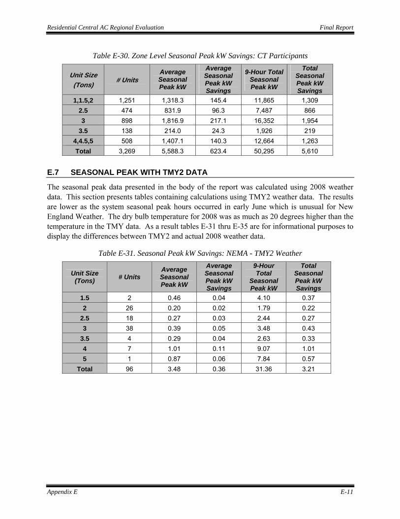
Residential Central AC Regional Evaluation Final Report
Appendix E E-11
Table E-30. Zone Level Seasonal Peak kW Savings: CT Participants
Unit Size (Tons)
# Units Average Seasonal Peak kW
Average Seasonal Peak kW Savings
9-Hour Total Seasonal Peak kW
Total Seasonal Peak kW Savings
1,1.5,2 1,251 1,318.3 145.4 11,865 1,309 2.5 474 831.9 96.3 7,487 866 3 898 1,816.9 217.1 16,352 1,954
3.5 138 214.0 24.3 1,926 219 4,4.5,5 508 1,407.1 140.3 12,664 1,263 Total 3,269 5,588.3 623.4 50,295 5,610
E.7 SEASONAL PEAK WITH TMY2 DATA
The seasonal peak data presented in the body of the report was calculated using 2008 weather data. This section presents tables containing calculations using TMY2 weather data. The results are lower as the system seasonal peak hours occurred in early June which is unusual for New England Weather. The dry bulb temperature for 2008 was as much as 20 degrees higher than the temperature in the TMY data. As a result tables E-31 thru E-35 are for informational purposes to display the differences between TMY2 and actual 2008 weather data.
Table E-31. Seasonal Peak kW Savings: NEMA - TMY2 Weather
Unit Size (Tons) # Units
Average Seasonal Peak kW
Average Seasonal Peak kW Savings
9-Hour Total
Seasonal Peak kW
Total Seasonal Peak kW Savings
1.5 2 0.46 0.04 4.10 0.37 2 26 0.20 0.02 1.79 0.22
2.5 18 0.27 0.03 2.44 0.27 3 38 0.39 0.05 3.48 0.43
3.5 4 0.29 0.04 2.63 0.33 4 7 1.01 0.11 9.07 1.01 5 1 0.87 0.06 7.84 0.57
Total 96 3.48 0.36 31.36 3.21

Residential Central AC Regional Evaluation Final Report
Appendix E E-12
Table E-32. Seasonal Peak kW Savings: WCMA - TMY2 Weather
Unit Size (Tons)
# Units Average Seasonal Peak kW
Average Seasonal Peak kW Savings
9-Hour Total
Seasonal Peak kW
Total Seasonal Peak kW Savings
1.5 2 0.36 0.03 3.28 0.30 2 26 0.12 0.02 1.09 0.15
2.5 18 0.43 0. 05 3.83 0.43 3 38 0.24 0.02 2.12 0.22
3.5 4 0.20 0.00 1.77 0.01 4 7 0.22 0.02 2.00 0.20 5 1 0.61 0.04 5.51 0.40
Total 96 2.18 0.19 19.60 1.70
Table E-33. Seasonal Peak kW Savings: SEMA – TMY2 Weather
Unit Size (Tons)
# Units Average Seasonal Peak kW
Average Seasonal Peak kW Savings
9-Hour Total
Seasonal Peak kW
Total Seasonal Peak kW Savings
1.5 2 1.01 0.09 9.10 0.83 2 26 0.44 0.05 3.99 0.49
2.5 18 0.59 0.07 5.28 0.59 3 38 0.75 0.09 6.78 0.82
3.5 4 0.97 0.11 8.76 0.98 4 7 1.36 0.14 12.25 1.30 5 1 2.85 0.21 25.69 1.87
Total 96 7.98 0.76 71.86 6.88
Table E-34. Seasonal Peak kW Savings: RI – TMY2 Weather
Unit Size (Tons)
# Units Average Seasonal Peak kW
Average Seasonal Peak kW Savings
9-Hour Total
Seasonal Peak kWh
Total Seasonal Peak kWh Savings
1.5 2 0.68 0.06 6.11 0.56 2 26 0.18 0.02 1.59 0.20
2.5 18 0.26 0.03 2.30 0.24 3 38 0.29 0.04 2.60 0.33
3.5 4 0.23 0.03 2.06 0.25 4 7 0.98 0.11 8.84 0.99 5 1 0.37 0.03 3.29 0.24
Total 96 2.98 0.31 26.79 2.80
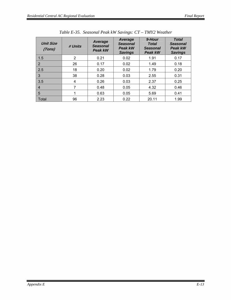
Residential Central AC Regional Evaluation Final Report
Appendix E E-13
Table E-35. Seasonal Peak kW Savings: CT – TMY2 Weather
Unit Size (Tons)
# Units Average Seasonal Peak kW
Average Seasonal Peak kW Savings
9-Hour Total
Seasonal Peak kW
Total Seasonal Peak kW Savings
1.5 2 0.21 0.02 1.91 0.17 2 26 0.17 0.02 1.49 0.18 2.5 18 0.20 0.02 1.79 0.20 3 38 0.28 0.03 2.55 0.31 3.5 4 0.26 0.03 2.37 0.25 4 7 0.48 0.05 4.32 0.46 5 1 0.63 0.05 5.69 0.41 Total 96 2.23 0.22 20.11 1.99

Appendix F F-1
APPENDIX F. DUCT LEAKAGE AND INFILTRATION TESTING
Besides incentives for installation of high efficiency air conditioning equipment, the sponsoring utilities also offered incentives for duct sealing and infiltration measures. To provide data that can be used in the evaluation of the effectiveness of such measures, duct pressurization testing was also conducted at the houses where operation of the air conditioning systems was monitored. The duct pressurization testing was conducted to provide data for measuring the following:
• Total duct leakage (in CFM);
• Duct leakage to unconditioned spaces (in CFM); and
• Total building infiltration rates (in air changes per hour-ACH).
F.1 SAMPLING PLAN FOR DUCT LEAKAGE TESTING
Testing for duct leakage and infiltration was conducted at 86 sites from among the sites in the whole sample. Tests for total duct leakage were completed at 70 of these sites. Tests for duct leakage to unconditioned spaces were completed for 78 sites. Testing was not feasible at some sites for various reasons, including ducts/vents not being accessible and homeowners not willing to have the testing performed. In addition, there were some houses that could not be properly pressurized.
F.2 TESTING PROCEDURES
To measure duct leakage, ADM field staff performed duct pressurization testing (using Duct Blasters®) on the ducting for central air conditioning systems. System static pressure (SSP) on the duct system was first measured, where SSP is a measurement of static pressure at the supply side plenum of the duct system when the supply fan is on and operating with registers in their normal position. This pressure is unique for each system. The ducts were then pressurized by means of a Duct Blaster® connected to the return side of the system. Total duct leakage was measured with the registers sealed and the Duct Blaster® pressurizing the duct system. Total Duct leakage at 25 Pa was then recorded.
An additional step was required to measure duct leakage to unconditioned space. A Blower Door® was set up in an exterior doorway and used to pressurize the house to the same pressure as the ducts. This prevented any leakage to other conditioned spaces within the residence; all leakage measured, once the home was pressurized, would therefore be only to unconditioned spaces. Duct leakage to unconditioned space was then measured at 25 Pa, where possible.
In some cases leaky house envelopes did not allow pressurization of the house to the target duct pressures. ADM field staff would then record the alternate pressure at which the test was performed. However results for such sites are not easily comparable to the majority of sites tested at 25 Pa. All figures for total duct leakage and duct leakage to unconditioned space are measured in cubic feet per minute (CFM). The procedure for duct blaster and blower door testing is detailed in Figure F-1 below.

Residential Central AC Regional Evaluation Final Report
Appendix F F-2
Finally, total home infiltration, measured in air changes per hour (ACH), was calculated. One-time measurements of pressure differential between the conditioned and unconditioned space were taken to calculate a snap shot of total home infiltration, in CFM. This, along with the residence’s volume, in cubic feet, was used to calculate total ACH of the envelope. However, this measurement of infiltration will not remain constant throughout the year, as it is a function of pressure differential between the interior and exterior of the home. As this pressure varies, with changing wind and outdoor temperatures, so will infiltration of the residence’s envelope.
Figure F-1 Duct Blaster and Blower Door Testing Diagram
Data for measuring duct leakage and infiltration were collected using a Duct Blaster® and a Blower Door®. For the testing, registers were sealed, a Duct Blaster® was connected to the return side of the system, and a Blower Door® was set up in an exterior doorway and used to pressurize the house to the same pressure as the ducts.
After making the duct leakage measurements, the field staff tested total home infiltration, measured in CFM. The ducts were sealed and one-time measurements of pressure differential between the conditioned and unconditioned space were taken to calculate a snap shot of total home infiltration. The measurements from duct blasting equipment are at an artificially high pressure differential, however, so for comparison to natural ambient pressure differential, a conversion factor is required. This conversion is as follows:
where

Residential Central AC Regional Evaluation Final Report
Appendix F F-3
50 Pascal is the base pressure used for comparison
Test Pressure = 25 Pascal (pressure at which tests were performed)
CFMmeasured = CFM reading from equipment
17 = Regional conversion factor for New England
.65 = Average slope of the “House Leakage Curve”1
The “House Leakage Curve” is a model developed by the makers of Minneapolis Blower Door based on a collection of data on individual home tests. This model, based on a long series of actual measurements, predicts what total home infiltration will be based on pressure differential between the inside and outside of a residence. The .65 figure is the average slope of the curve for tests at 50 Pa. The equation includes a correction for testing at pressures other than 50 Pa., so changing the exponent is not necessary. Though the exponent value will differ for individual homes, for a statistically significant sample the .65 figure is an accurate average.
The CFM data was used along with the residence’s volume to calculate total ACH of the envelope, per this equation:
ACH = CFMambient*60/Volume
It should be noted that the measurement of total home infiltration is accurate only for the pressure differential at the time the test was performed. Variations in pressure differential between the interior of the home and outside of the home will cause this measurement of total infiltration to change throughout the year. However, the pressure differential at the time of our field testing should be sufficiently representative of the pressure differential typical of the peak summer cooling season.
In the interviews that were conducted as part of the on-site data collection, field staff asked residents how long it had been since the ducting system was serviced. There were very few instances of recent repair.
1 See Minneapolis Blower Door Operation Manual