Environment and Sustainable Development Department (ENDESA)

RESERVOIRS AND CLIMATE CHANGE

INTRODUCCIÓN10

RESERVOIRS AND CLIMATE CHANGE

November 2008

Authors:Antoni Palau1 and Miguel Alonso2

1 Environment and Sustainable Development Department ENDESA.2 URS (United Research Services España, S.L.)

CONTENTS

FOREWORD 5

I. INTRODUCTION

1. GENERAL CLIMATE FEATURES 8

2. CONTEMPORARY CLIMATE CHANGE 10

3. THE GREENHOUSE GASES N2O, CO2 AND CH4 11

4. GLOBAL WARMING AND GLOBAL DIMMING 13

II. HYDROELECTRICITY IN THE GLOBAL ENERGY BALANCE

1. INTRODUCTION 15

2. ENERGY PRODUCTION AND CONSUMPTION IN SPAIN 15

3. THE ROLE OF HYDROELECTRICITY IN MEETING THE DEMAND FOR ENERGY 16

4. HYDROELECTRICITY AND OTHER ENERGY SOURCES IN TERMS OF CO2 BALANCE 18

III. AQUATIC ECOSYSTEMS AND GREENHOUSE GASES

1. CARBON 21

2. NITROGEN 22

3. RESERVOIRS AND GREENHOUSE GASES 22

IV. A CASE STUDY: THE SUSQUEDA RESERVOIR (TER RIVER, GIRONA)

1. INTRODUCTION 32

2. STUDY APPROACH 33

3. FIELD METHODS 34

4. ANALYTICAL METHODS 36

5. RESULTS 36

6. FINAL BALANCE 41

7. DISCUSSION OF RESULTS 42

V. SOME IMPORTANT FINAL QUESTIONS 44

BIBLIOGRAPHY 47

FOREWORD

The purpose of this publication is to analyze the role of reservoirs in the dynamics

of greenhouse gases in order to highlight how they are involved in climate change. The

analysis is carried out by describing their metabolism as aquatic systems. We illustrated

this description by a case study of the Susqueda Reservoir (Ter River), which focuses on

its carbon balance.

Previously, we review the situation of climate change, starting with the discussion of the

concept of climate and its natural variability. We provide a brief account of the factors and

processes that have contributed, and still contribute, to the global and regional evolution of

the Earth’s climate on both a geological and contemporary time scale.

In one of the chapters, we address the role of hydroelectricity in the overall energy balance.

We analyze the relationship between available energy, the production of regulable energy

by reservoirs, and the energy usage and demand by Spanish today`s society. We also

make a brief comparison of hydroelectric energy with other electricity-generating technolo-

gies in relation to climate change.

I

INTRODUCTION

1. GENERAL CLIMATE FEATURES

Climate is perhaps the most important factor in biological evolution

and in the history of mankind. It has always been a decisive factor

for the survival and economy of the people. We know that climate is

related to sunlight, air temperature, winds, atmospheric humidity and

rainfall. However, to avoid confusion about the meaning of “climate

change”, we should perhaps define the term ‘climate’, as it is often

used incorrectly to refer to “weather” or “atmospheric conditions”. A

very precise and accurate version is given by Inocencio Font Tullot1,

one of the most prestigious Spanish meteorologists: “Climate is the

synthesis of the fluctuating set of weather conditions in a given area

recorded during a long period enough to be geographically represent-

ative”. This definition includes key concepts in the current perception

of climate change by society:

• The parameters used to define climate have large variations.

• Climate is spatially dependent.

• Very long periods of time are necessary to guarantee that a climate

analysis is representative or significant.

The identification of regular features of climate in different areas of

the earth’s surface has led to classifications based on combinations

of elements that have been expressed in geographical terms. These

classifications are mainly based on atmospheric and marine circula-

tion, latitude and altitude. In other words, we have climatic maps. How-

ever, these maps show major inaccuracies at the boundaries between

climate zones and only help to understand climate-dependent proc-

esses, such as the organization of vegetation, at a particular spatial

and temporal scale. In the short term, the farmer still relies on sky

observation.

In addition to the great difficulty of accurately predicting climate to

be able to organize our economy suitably, it also changes over time.

Throughout the history of the world there have occurred very great

variations in climate associated with continental drift and its effects

on the configuration and circulation of the hydrosphere. The lands

that today make up the Iberian Peninsula travelled over the South

Pole about 500 million years ago and over the equator about 300

million years ago. In the Cenozoic Era, the Earth’s geography was

established more or less as we know it today. This was a period of

cooling, when the formation of the Isthmus of Panama led to the def-

inition of the polar ice caps and the onset of glaciations—a climatic

phenomenon that had only been previously recorded in the Permian.

During the Pleistocene there have been four glacial periods, when

ice covered a third of the continents and turned temperate climates

into Arctic ones. The last glacial period ended only about 10,000

years ago. However, the traditional concept of the “four glacials”

conceals a more complex situation. In fact, during these major

glacials thirty or more intermediate pulses of glacial advance and

retreat have been identified, each of them lasting about 43,000

years. Furthermore, within these intermediate pulses there were

smaller ones lasting between 19,000 and 24,000 years. Super-

imposed on these pulses, even smaller changes in climate are re-

corded, like those occurred between the 10th and 14th centuries,

known as the Medieval Warm Period. This period was warmer than

the present, but it was followed in the 16th and 17th centuries by

the Little Ice Age, which despite its name was of great importance

in History (Figure 1).

Because of the periodicity of the Pleistocene glaciations, many

studies have attempted to situate the present time within another

interglacial cycle. We wish to know whether we are going towards

a fifth glacial period, and if so whether we are still in the warm-

ing phase or moving towards the cooling phase. Several soundly-

based scientific theories have been developed to explain the past,

but their predictive accuracy is not demonstrable. According to

the series of Milankovitch cycles, we are at the end of the current

interglacial warm period, so the Earth should start cooling. The Mi-

lankovitch theory states that the Earth’s orbit varies from almost

circular to clearly elliptical every 90,000 or 100,000 years, so the

intensity of sunlight received by Earth varies. Superimposed on this

variation are those of precession and the changes in the tilt of the

Earth’s rotational axis, which have a cycle of 43,000 years: when

the tilt is greater, the magnitude of the seasonal change from win-

ter to summer is accentuated. This interval fits with the duration

of the intermediate pulses of glacier advance and retreat, but the

timing of the fluctuations is irregular, so other factors must be in-

volved. W.M. Ewing2 proposed a mechanistic model of cyclical phe-

nomena based on the relationships between the atmosphere and

INTRODUCTION8

1 Inocencio Font Tullot, a highly active and prolific Spanish meteorologist who started his career at the Izaña Observatory, have managed several relevant international meteorology projects. In 1974 he was appointed Director of the National Meteorology Service. He wrote Climatología de España y Portugal (Climatology of Spain and Portugal, 1983) and Historia del Clima en España (A History of Climate in Spain, 1988).

2 William Maurice Ewing, an American geologist and professor of Columbia University, who in the 1950s proposed a theory on the possible causes of glaciations, and the hypothesis that the glacial periods were only a recent stage in the geological and climatic history of the Earth.

the hydrosphere. In an interglacial period with an ice-free Arctic

Ocean, the temperature would be low though slightly higher than

at the present time. However, evaporation would be large, provok-

ing heavy snowfall that would accumulate into continental glaciers

which increases the albedo of Earth’s surface. The drop in sea level

associated with this process would isolate the polar basin of the

Atlantic, which would lower water temperature, keep ice in solid

state and reduce precipitation. This would make the glaciers re-

treat again, and climate would return to interglacial conditions.

On a different scale of time and importance, other factors such as

solar activity and volcanoes also act on climate. Solar activity may

have increased in the last 200-300 years, in turn causing an in-

crease in the thermal radiation that reaches the Earth. Sunspots,

which are colder parts of the Sun’s surface linked to greater mag-

INTRODUCTION9

Figure 1. Evolution of atmospheric temperature across different temporal scales. The increase in human population, coinciding to the temperature increase during the last two centuries, is also depicted.

INTRODUCTION10

netic activity, increase and decrease with a periodicity of about

11 years, with primary cycles of 9 to 14 years and secondary cycles

of about 80 years. However, the reduction in the energy emitted

by sunspots is compensated by the intensification of the surround-

ing bright areas, or faculae, so the larger the area occupied by

sunspots, the more intense the solar activity is. In January 2008

the European/US SOHO satellite detected the appearance of a

new sunspot. This phenomenon has been interpreted as indicating

the start of a new solar cycle that will cause a gradual increase in

sunspots and solar flares, reaching a peak of activity between 2011

and 2013.

The relationship between sunspots and climate is subject to

debate. Some scientists attribute climate change to cycles of

solar activity rather than to the concentration of CO2 in the at-

mosphere. Without going into whether or not there is a causal

relationship, the fact is that total solar radiation has increased

in recent centuries (Figure 2). The Maunder Minimum—the name

given to a period of almost 50 years with hardly any sunspots

(1645-1715)—coincided with the coldest time of what is known

as the Little Ice Age, with very cold winters at least in the north-

ern hemisphere. The particles expelled by volcanoes can reach

the stratosphere in sufficient amounts to intercept the radiant

energy and cause cooling.

slowly, leading to heat increase in the air inside. The atmosphere

can be compared to this system: the gases usually found in it,, such

as water vapor, carbon dioxide (CO2), methane (CH4) and ozone—

together with pollutants such as nitrous oxide (N2O) and CFCs—trap

the infrared radiation that is radiated back into space by the hydro-

sphere and the lithosphere when heated by solar radiation. In the

absence of these gases and the predominant nitrogen and oxygen,

Earth would not be protected from violent thermal changes and

from extreme cold, and life as we know would be impossible.

But what are the effects of climate change in the past and in the fu-

ture? They are decisive in the history of the biosphere and particular-

ly in the history of humanity. The climate has governed the complex

and dynamic puzzle of the evolution of species and their distribution

on the planet. Many large extinctions can be traced to some sudden

climatic changes, even as far back as the end of the Mesozoic, when

a sudden cooling of the climate caused by the impact of a huge me-

teorite wiped out the dinosaurs and many plants but was favourable

to mammals and seed-bearing plants. The Pleistocene glaciations

had a particularly devastating effect on the continents with east-west

mountain ranges, which prevented the movement of populations to

the south as the cold advanced. The sea could have fallen down to

120 m below the current level. Global warming in the Boreal period

was decisive for the birth of the Neolithic Age, particularly in Spain,

where rainfall decrease decimated the herds of wild ruminants, so

humans had to adapt by enhancing their ability to intervene in the

environment. Later, great civilizations such as those in North Africa,

the Indus Valley and Mesopotamia rose and fell under the influence

of climate changes. The Little Ice Age in the 16th and 17th centuries

ruined the wool trade and the textile industry in both Castiles and

fostered the resurgence of Catalonia. After the experience of the

last few decades, we are very aware of the effect of cycles of wet and

dry years and cool and warm periods on the Spanish economy and

on the health and welfare of the population.

2. CONTEMPORARY CLIMATE CHANGE

Though humanity is aware of the natural tendency of climate changes,

the current concern is whether economic activities will make these

changes so sudden that could catch us unawares and without sufficient

time and means to adapt. And within climate change, the most tangi-

ble aspect is global warming. This phenomenon presumably arises as

a direct consequence of economic development based on combus-

Figure 2. Evolution of solar radiation intercepted by Earth, which have in-creased in the last centuries (data from Lean, 2004).

Greenhouse gases, which are the main subject of this publication,

are another factor that affects climate. They are named after the

glasshouses that maintain a warm atmosphere inside them using

only sunlight. The short-wave electromagnetic radiation from the

sun enters the greenhouse through the glass or plastic surfaces,

but the longewave infrared radiation leaves the structure more

INTRODUCTION11

tion of coal, oil and natural gas, which has been growing continuously

since the early twentieth century. The main substance released in the

combustion reaction of these products is carbon dioxide (CO2), one

of greenhouse gases. Based on isotope discrimination techniques,

it has been concluded that this combustion has led to the increase

in atmospheric CO2; the atmospheric gas is lacking in C14, which is

lower in fossil fuels, due to its reduced half-life of between 5,500 and

6,000 years. Furthermore, the measuring station of atmospheric

CO2, which has been collecting data at Mauna Loa (on the Hawaiian

Tropic of Cancer) since 1958, shows a steady increase up to the

present that runs parallel with the global consumption of fossil fuels.

Agricultural activities such as deforestation and draining of wetlands

also release CO2. Overall, it is considered that the CO2 produced

through all the above processes is twice the retained in the atmos-

phere. The carbon sink of the other half could be the ocean and per-

haps the vegetation. However, although in the long term this might

be possible, the speed at which the CO2 is being produced is clearly

leading to its accumulation in the atmosphere. CH4 is also showing

considerable increases (around 1% per year) attributed to increased

livestock production and creation of new anaerobic aquatic environ-

ments such as rice fields.

Between 1856 and 2000 the global temperature increased be-

tween 0.4 and 0.8ºC. However, since 1975 the correlation be-

tween the increases in temperature and CO2 has been greater. The

Intergovernmental Panel on Climate Change (IPCC) has undertaken

the task of modelling the future evolution of temperature in differ-

ent scenarios depending on whether society comes out in favour

of the economy or the environment, and in each case whether the

actions are taken at a global or regional level. Estimates of the cli-

matic consequences of the different scenarios show increases in

temperature of 2ºC to 4.5ºC and sea level rise between 31 and

49 cm by 2100.

Without questioning the hard data of increased atmospheric CO2 and

rising temperature, some experts do question the predictive value

of the IPCC’s models. Their doubts are based mainly on whether we

know the true effect of CO2 on temperature, whether there may be

other factors involved in the increase in temperature that have not

been considered, and whether we know the true qualitative and quan-

titative consequences of the increase. These questions are very dif-

ficult to consider scientifically because of the enormous complexity of

the physical, chemical and mechanical processes taking place in the

Earth’s fluid envelopes. Though the temperature and the evolution

of human population follow similar temporal patterns (see Figure 1),

the relationships between the physical and biological world are not

always causal or easy to establish.

There is an amusing classical example to criticize the use of correla-

tions to establish simplistic cause-effect relationships. A study con-

ducted between 1970 and 1980 could be used to attribute the fall-

ing birth-rate in Poland to the reduction in stork populations, whereas

in reality the processes involved in this coincidence were of far great-

er socioeconomic and environmental importance: the industrializa-

tion of the country resulted on the one hand in the incorporation of

women into employment, and on the other hand in the degradation

of the habitat of storks.

3. THE GREENHOUSE GASES N2O, CO2 AND CH4

Nitrous oxide (N2O) is present in the atmosphere in a concentration

of about 300 ppm and has been increasing recently by 2% per year.

This gas makes little contribution to the greenhouse effect due to its

Figure 3. Sustained increase in atmospheric CO2 concentration over the last fifty years. Annual fluctuation due to the seasonality of photosynthetic activity in the northern hemisphere can be clearly observed.

very slight concentration in the atmosphere, though it has a ther-

mal potential 310 times greater than that of CO2. Nitrous oxide is

produced as an intermediate in the denitrification process that oc-

curs in anaerobic environments with sufficient availability of oxidizable

organic matter and nitrate, and also as a result of burning biomass

and fossil fuels. The two main nitrous oxide sinks are the fixation by

nitrifying organisms, which can use nitrous oxide as an alternative to

nitrogen, and the reaction with atomic oxygen in the stratosphere,

which is the most important mechanism of removal of this gas from

the atmosphere.

Carbon dioxide (CO2) and methane (CH4) are the most stable car-

bon gases. CO2 is the most abundant of these gases, but currently

only represents 0.038% of the atmosphere. CH4 is only considered

a trace gas but has a greenhouse effect 20 times greater than CO2.

Atmospheric CO2 is in equilibrium with the bicarbonate of the hydro-

sphere, which is the most important carbon store on the planet. The

direction of the shift from one to another system is governed by the

CO2 pressure in the atmosphere and the bicarbonate concentration

in the water. However, apart from these purely physical aspects, the

biogeochemical carbon cycle includes complex redox processes in-

volving living organisms. Both bicarbonate and CO2 are reduced to

organic molecules by photosynthetic organisms using solar energy,

which is the way carbon enters the biosphere. Subsequently, the or-

ganic molecules are oxidized by oxygen or other terminal electron

acceptors. The return to the initial oxidized form, i.e. CO2, may follow

long and tortuous routes depending on the complexity of the ecosys-

tems and the involvement of other mechanisms, which may include

geological processes. Some of the CO2 is fixed by plants and rapidly

returned to the atmosphere or to the water through respiration or

decomposition of organic matter in the ecosystems; some was fixed

in ancient times and is stored as wood, coal, oil, natural gas or even

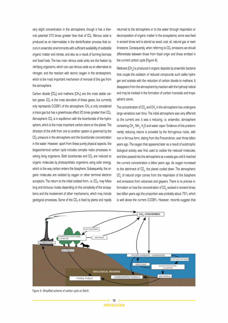
limestone. Consequently, when referring to CO2 emissions we should

differentiate between those from fossil origin and those emitted in

the current carbon cycle (Figure 4).

Methane (CH4) is produced in organic deposits by anaerobic bacteria

that couple the oxidation of reduced compounds such aslike hydro-

gen and acetate with the reduction of carbon dioxide to methane. It

disappears from the atmosphere by reaction with the hydroxyl radical

and may be involved in the formation of carbon monoxide and tropo-

spheric ozone..

The concentration of CO2 and CH

4 in the atmosphere has undergone

large variations over time. The initial atmosphere was very different

to the current one: it was a reducing, i.e. anaerobic, atmosphere

containing CH4, NH

3, H

2S and water vapor. Evidence of this predomi-

nantly reducing nature is provided by the ferruginous rocks, with

iron in ferrous form, dating from the Precambrian, over three billion

years ago. The oxygen that appeared later as a result of autotrophic

biological activity was first used to oxidize the reduced molecules,

and then passed into the atmosphere as a waste gas until it reached

the current concentration a billion years ago. As oxygen increased

to the detriment of CO2, the planet cooled down. The atmospheric

CO2 of natural origin comes from the respiration of the biosphere

and emissions from volcanoes and geysers. There is no precise in-

formation on how the concentration of CO2 evolved in ancient times;

two billion years ago the proportion was probably about 75%, which

is well above the current 0.038%. However, records suggest that

INTRODUCTION12

Figure 4. Simplified scheme of carbon cycle on Earth.

during the interglacial periods the temperature increase was ac-

companied by a significant increase in CO2, which is logical if one

considers in accordance withthat the higher water temperature of

the hydrosphere was warmer and therefore had aits lower capacity

to dissolve gases.

Aquatic systems have played a decisive role in the changes in com-

position of the atmosphere. Oxygen comes from photosynthesis, and

the first organisms to use this way of carbon incorporation were simi-

lar to the current cyanobacteria, inhabiting shallow and probably very

eutrophic seas three and a half billion years ago.

4. GLOBAL WARMING AND GLOBAL DIMMING

In the last few decades, policies, investments and business have been

driven by major global issues, particularly those that can have cata-

strophic effects. Some of them are still great causes of concern (the

hole in the ozone layer, global warming), while others have been left

behind (the nuclear threat during the Cold War, meteorite impact)

but may reappear at any time.

The major issue at present is global warming, probably for three

reasons: First, it is very difficult to quantify and predict, so an infinite

number of hypotheses and theories have emerged to satisfy all pos-

sible opinions. Second, related to the first but with a greater impact

on society, any meteorological event can be claimed to be the result

of global warming: now it rains more, now it rains less, it is hotter than

before or colder than before, the winters are not so cold, etc. Third,

the effects are predicted in the medium and long term (50 years or

more), so none of the prophets can be taken to task.

However, an increasing number of experts are sceptical on the

effects of climate change, and even on its relationship to human

activities. Another major global issue is therefore needed, and “global

dimming” is well placed to gain favour.

Indeed, pollutant emissions from human activities of combustion

not only introduce greenhouse gases into the atmosphere, as dis-

cussed above. They also emit many particles like ash and soot, which

intercept part of the solar radiation reaching the earth’s surface. It

seems that in certain parts of the world this radiation and the rate

of evaporation have decreased measurably, in spite of global warm-

ing. The hypothesis to explain this is that the suspended particulate

INTRODUCTION13

contaminants block the solar radiation and convert the clouds into

giant mirrors. The greater the number of particles in suspension,

the greater the number of condensation nuclei for water droplets

to form, the smaller these droplets are, the higher the density of

the clouds, and the greater the screening (mirror) effect they have

against solar radiation. Some scientists suggest that solar radiation

reaching the Earth’s surface has been reduced by between 6% and

30%, depending on the considered zone. According to those who sup-

port this theory, these “mirror” clouds alter the distribution of rainfall

on the planet by cooling the oceans, as—they claim—occurred in the

northern hemisphere in the 1970s and 1980s. Greater evaporation

intensify drought.

Global dimming thus acts in the opposite direction to global warming:

the former cools and the latter heats. We thus have the following

paradox: if we avoid particulate pollution in the atmosphere, the global

dimming effect will decrease, thus reinforcing global warming. Put

another way, thanks to global dimming the effects of global warming

have so far been reduced, but if we reduce the causes of global dim-

ming (which is being done by using particle filters in power stations

and internal combustion engines), global warming will have no limit.

Its effects would be even more devastating than expected because

the current prediction models do not take this process into account.

Average temperature increases of 10ºC are being predicted for the

end of the 21st century.

One option is to immediately stop eliminating the particles emitted

into the atmosphere by combustion processes in order to keep the

effects of global dimming active and thus delay or mitigate the apoca-

lyptic effects of global warming. Howver, it is surprising that the pro-

ponents of the global dimming theory fail to appreciate the contribu-

tion of suspended particles to global warming, which is undoubtedly

not negligible. It can also be assumed that a high concentration of

“protective” suspended particles in the atmosphere would affect the

respiratory processes of many life forms, among other effects.

The fact that assumptions and theories lead to such simple and ob-

vious paradoxes is indicative of enormous gaps in our knowledge,

particularly on the regulatory processes involved in the nature and

functioning of natural ecosystems. Therefore, it might be argued that

if global dimming is important, part of the current climate change

may be due to the sharp reduction in the concentration of suspended

particles in the atmosphere in comparison with the late 19th century,

when the use of coal as a fuel was widespread.

II

HYDROELECTRICITY IN THE GLOBAL ENERGY

BALANCE

HYDROELECTRICITY IN THE GLOBAL ENERGY BALANCE15

1. INTRODUCTION

Reservoirs store water that can be used for a variety of purposes

and host complex aquatic ecosystems. Furthermore, they play a very

important role in the production of energy through hydroelectricity.

Before analyzing how—and to what extent—reservoirs are involved in

the greenhouse effect, we will explain the important role of hydroelec-

tric power in the global energy balance and the key role that it plays

in the energy organization of countries that are highly dependent on

both water and energy like Spain.

2. ENERGY PRODUCTION AND CONSUMPTION IN SPAIN

Spain is an energy-poor country that imports more than 80% of the

consumed energy. This is probably a little known fact, although it is

the key to understand current energy management in Spain and to

raise public awareness about the importance of saving energy. To

be exact, 139.5 x 106 tonnes of oil equivalent (toe) were imported

in 2005, showing a 7.7% rise over 2004 and representing 85.1%

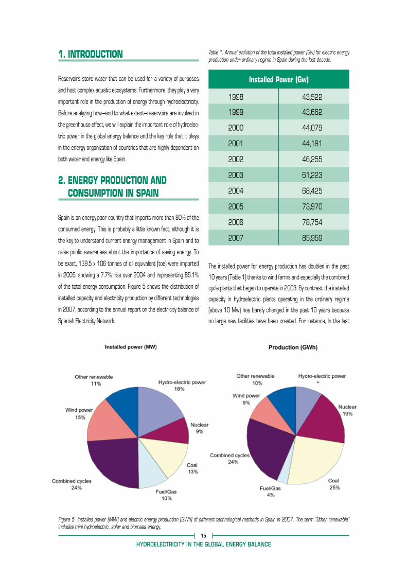
of the total energy consumption. Figure 5 shows the distribution of

installed capacity and electricity production by different technologies

in 2007, according to the annual report on the electricity balance of

Spanish Electricity Network.

The installed power for energy production has doubled in the past

10 years (Table 1) thanks to wind farms and especially the combined

cycle plants that began to operate in 2003. By contrast, the installed

capacity in hydroelectric plants operating in the ordinary regime

(above 10 Mw) has barely changed in the past 10 years because

no large new facilities have been created. For instance, In the last

Figure 5. Installed power (MW) and electric energy production (GWh) of different technological methods in Spain in 2007. The term “Other renewable” includes mini hydroelectric, solar and biomass energy.

Table 1. Annual evolution of the total installed power (Gw) for electric energy production under ordinary regime in Spain during the last decade.

Installed Power (Gw)

1998 43,522

1999 43,662

2000 44,079

2001 44,181

2002 46,255

2003 61,223

2004 68,425

2005 73,970

2006 78,754

2007 85,959

HYDROELECTRICITY IN THE GLOBAL ENERGY BALANCE16

5 years, it has remained stable at 16,658 MW. This has reduced

largely the percentage share of hydroelectricity in total electric power

production: from 37.8% in 2000 to 19.4% in 2007. In the coming

years new hydroelectric pumping projects will involve a power in-

crease of about 3000 MW, MW corresponding to projects that are

already in place.

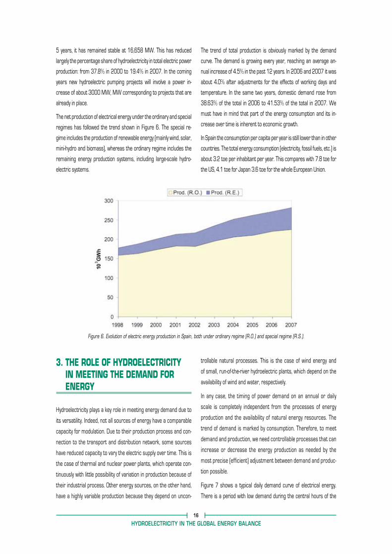
The net production of electrical energy under the ordinary and special

regimes has followed the trend shown in Figure 6. The special re-

gime includes the production of renewable energy (mainly wind, solar,

mini-hydro and biomass), whereas the ordinary regime includes the

remaining energy production systems, including large-scale hydro-

electric systems.

The trend of total production is obviously marked by the demand

curve. The demand is growing every year, reaching an average an-

nual increase of 4.5% in the past 12 years. In 2006 and 2007 it was

about 4.0% after adjustments for the effects of working days and

temperature. In the same two years, domestic demand rose from

38.63% of the total in 2006 to 41.53% of the total in 2007. We

must have in mind that part of the energy consumption and its in-

crease over time is inherent to economic growth.

In Spain the consumption per capita per year is still lower than in other

countries. The total energy consumption (electricity, fossil fuels, etc.) is

about 3.2 toe per inhabitant per year. This compares with 7.8 toe for

the US, 4.1 toe for Japan 3.6 toe for the whole European Union.

Figure 6. Evolution of electric energy production in Spain, both under ordinary regime (R.O.) and special regime (R.S.).

3. THE ROLE OF HYDROELECTRICITY IN MEETING THE DEMAND FOR ENERGY

Hydroelectricity plays a key role in meeting energy demand due to

its versatility. Indeed, not all sources of energy have a comparable

capacity for modulation. Due to their production process and con-

nection to the transport and distribution network, some sources

have reduced capacity to vary the electric supply over time. This is

the case of thermal and nuclear power plants, which operate con-

tinuously with little possibility of variation in production because of

their industrial process. Other energy sources, on the other hand,

have a highly variable production because they depend on uncon-

trollable natural processes. This is the case of wind energy and

of small, run-of-the-river hydroelectric plants, which depend on the

availability of wind and water, respectively.

In any case, the timing of power demand on an annual or daily

scale is completely independent from the processes of energy

production and the availability of natural energy resources. The

trend of demand is marked by consumption. Therefore, to meet

demand and production, we need controllable processes that can

increase or decrease the energy production as needed by the

most precise (efficient) adjustment between demand and produc-

tion possible.

Figure 7 shows a typical daily demand curve of electrical energy.

There is a period with low demand during the central hours of the

Figure 7. Distribution of different energy sources supplying the medium power demand curve in a typical day.

HYDROELECTRICITY IN THE GLOBAL ENERGY BALANCE

night, from 2 to 6 a.m., followed by an initial peak demand between

11 and 13 a.m. and a higher and longer peak between 4 and 9 p.m.

These time differences in energy requirements are obviously related

to social habits (work schedules, domestic and industrial activities,

etc.). The daily demand curve is established from one day to the

next by a forecasting model based on historical data and variation

trends.

To meet the daily demand curve, the managing body of the elec-

tricity market gives priority first to the production processes that

are most difficult to modulate (nuclear) or regulate (wind and run-

of-the river hydroelectric power). There follows thermal produc-

tion (coal, fuel-oil, gas, combined cycle), which has a very limited

capacity for regulation. The only energy source that can fine-tune

production to demand is conventional hydroelectric power (with

regulation).

The use of conventional hydroelectric plants associated with large

reservoirs and the support of reversible hydroelectric plants (pump

turbines), allows electric production to be adjusted precisely to the

daily demand curve. For example, in a situation of failure in a thermal

or nuclear plant, the only energy source that can compensate for the

fall in production quickly enough is conventional regulated hydroelec-

tricity (conventional or pumped).

Regulated hydroelectric production is also the only one that can

compensate for the fluctuations in production that can occur in the

course of a day in renewable energy sources that depend on natural

processes such as wind (very important in Spain), solar energy or

run-of-the-river hydroelectric power. When a wind farm stops pro-

duction due to lack of wind or feeds electricity into the grid due to

availability of wind, this is compensated precisely by hydroelectric

power stations feeding electricity in or drawing it out, respectively.

This regulatory role of hydroelectric plants also adds quality to the

energy supply because it allows a constant frequency (hertz) to be

maintained by compensating for the fluctuations in the grid according

to consumption.

Hydroelectric pumping stations add additional capabilities in the

management of electricity. These facilities consist of two reservoirs

located at different altitudes and connected by a hydroelectric plant

that can act as a pump or turbine as needed. When the consump-

tion of energy is minimal (at night), the surplus production can be

used to pump water to the upper reservoir, increasing the poten-

tial energy storage. When demand increases in the middle of the

day, the water accumulated during the night can be run through the

turbines in the hydroelectric plants, thus optimizing the production

and providing a good adjustment to the demand curve. These plants

17

HYDROELECTRICITY IN THE GLOBAL ENERGY BALANCEHYDROELECTRICITY IN THE GLOBAL ENERGY BALANCE18 19

are also an essential complementary system for optimizing energy

resources when the installed capacity of renewable sources is high,

as is the case with wind energy in Spain. In periods of high wind and

low demand for electricity, the wind power production can also be

used for pumping.

4. HYDROELECTRICITY AND OTHER ENERGY SOURCES IN TERMS OF CO2 BALANCE

Hydroelectric energy—like wind energy, photovoltaic energy and nu-

clear energy—is one of the sources that emits the least CO2 into the

atmosphere. However, we must consider in the emission assess-

ment of emissions not only the production process but also the full

life cycle of industrial production facilities (manufacture, construc-

tion, maintenance, demolition, etc.). In the case of hydroelectric-

ity, the type of facility (run-of-the-river, large reservoir, etc.) and the

hydro-morphological and biological characteristics of the water body

involved are of particular importance. In hydroelectric plants that

use large reservoirs, one must also take into account the types of

natural communities that they replace and their potential capacity

as carbon sinks.

Yield is an important factor in the energy production by different tech-

nologies. The yield is 33% for a nuclear power plant, 38.5% for a

thermal power plant and 90% for a hydroelectric power station. In

comparative terms, for each GWh of hydroelectric energy, we avoid

burning 223 t of oil, 248 hm3 of natural gas, 319 t of coal or 25 kg

of natural uranium.

Table 2 lists the emission of greenhouse gases related to the life

cycle of different electricity production technologies. The emissions

Table 2. Greenhouse gases emission during life cycle for different technologies of electric energy production.

Type of power plant Range (g CO2 eq/kWh) Mean value

Combined cycle (sinthetic coal gas)

Combined cycle (natural gas)

Hydroelectric (boreal reservoirs)

763-833

469-622

8-60

798

545

36

Coal (modern plant)

Diesel

Photovoltaic

959-1.042

555-880

12,5-104

1.000

717

58

Wind 7-22 14

from hydroelectric production are slightly higher than those from

wind power, similar to photovoltaic energy and far below those of

natural gas combined cycles, which are the options with least emis-

sions among fossil fuel technologies. In comparison with fossil fuel

power plants that use fuel-oil and carbon, each GWh produced by

a hydroelectric plant avoids emitting into the atmosphere between

450 and 1000 tonnes of CO2.

With regard to inland aquatic ecosystems and the production of

renewable energy, two European Directives must be respected in

conjunction. First, the Water Framework Directive (2000/60/

EC) aims to achieve by 2015 a “good ecological status” (or good

ecological potential for heavily modified water bodies) in all con-

tinental aquatic systems. Second, the Renewables Directive

(2001/77/EC) on the promotion of electricity from renewable

HYDROELECTRICITY IN THE GLOBAL ENERGY BALANCEHYDROELECTRICITY IN THE GLOBAL ENERGY BALANCE18 19

energy sources establishes the aims that, by 2010, renewable en-

ergy sources will provide 12% of the unprocessed primary energy

consumption (gross national consumption) in the EU and 29.4%

of total electricity generation in Spain. In 2007 renewable energy

achieved a 7% share of primary consumption, with an average an-

nual increase of 0.5%. At this increasing rate, in 2010 the figure

will be 8.5%—far from the 12% target. Obviously, in compliance

with the Renewables Directive, a significant role is played by the

development of hydroelectric power, which often affects the eco-

logical quality of the water bodies involved. It will be necessary to

apply the best strategies and technologies available to achieve the

objectives proposed in the two Directives.

III

AQUATIC ECOSYSTEMS AND GREENHOUSE GASES

AQUATIC ECOSYSTEMS AND GREENHOUSE GASES21

1. CARBON

Carbon enters aquatic systems through the dissolution of atmos-

pheric CO2. It is also a component of the particulate and dissolved

organic and inorganic matter that comes from their basins (Figure

8).The amount of atmospheric CO2 dissolved in water depends on

water temperature and acidity and the difference between atmos-

pheric CO2 partial pressure and concentration in the water (mainly

as CO2 and bicarbonate), which must end in equilibrium. As water

pH increases, the dissolved CO2 transforms first into gas, followed

by carbonic acid, bicarbonate and carbonate, in that order. If calcium

is present, it tends to form Ca CO3, which has low solubility and pre-

cipitates chemically, creating a carbon sink. Through photosynthesis,

CO3 and the HCO3- form part of the aquatic vegetation in the form

of phytoplankton, macrophytes or phytobenthos. From then on the

complexity of the cycle may vary.

Part of the assimilated carbon is rapidly released as CO2 by res-

piration of the vegetation. The rest is circulated through the food

web in zooplankton, zoobenthos, birds, fish and bacteria. It is also

returned to the water through the respiration of each compart-

ment and can be reused by autotrophs. If the CO2 partial pressure

in the water exceeds that of the atmosphere, it returns to the at-

mosphere.

Part of the assimilated carbon can be deposited in mineral form or

be chemically reduced in anaerobic sediments. A fraction may also be

transformed into methane through the reduction of carbon dioxide

when the conditions are suitable. Methane can be further oxidized to

carbon dioxide in the water and follow its pathway or be released into

the atmosphere. The biogeochemical carbon cycle varies according

to the dominant metabolic pathways. Autotrophy-dominated systems

are those in which the main carbon source is inorganic (CO2 or par-

ticulate or dissolved inorganic matter).

In general the dominant pathway followed by carbon in aquatic eco-

systems is that of autotrophy, in which the atmospheric CO2 enter-

ing the water is fixed by photosynthetic organisms. If the system is

oligotrophic, carbon cycling in the water body is closed and there is

little exchange with the atmosphere and sediments. However, if the

system is eutrophic, its role as a scavenger of atmospheric CO2 is

enhanced because the carbon cycle is opened to the sediment (Figu-

re 9). Finally, if the system is heterotrophic, carbon is mostly taken up

in organic form. Respiration of animals or bacteria is dominant in these

systems, so they release CO2.

Figure 8. Carbon cycle in aquatic ecosystems.

Figure 9. Carbon cycle in oligotrophic (closed) and eutrophic (opened) aquatic ecosystems.

2. NITROGEN

TThe nitrogen cycle in aquatic ecosystems is very complex and is regu-

lated by the redox potential in the different compartments of the water

body. In the presence of light, autotrophs in general are able to use all

forms of nitrogen, from molecular nitrogen to nitrate, incorporating it

into the food chain. In the decomposition stage, the nitrogen in the or-

ganisms is oxidized by bacterial action. If oxygen is present, correspond-

ing to a high redox potential, nitrate is produced through the action of

nitrifying bacteria, which are aerobic. However, if the oxygen is depleted,

the decomposition process of organic matter continues with fermenta-

tion, leading to the appearance of denitrifying bacteria (among others)

that use oxidized nitrogen molecules as terminal electron acceptors.

In other words, instead of oxygen they “breathe” nitrite and nitrate, and

this metabolism produces N2 and N2O, which can be released into the

atmosphere or incorporated again by nitrogen-fixing organisms such as

cyanobacteria in the water or bacteria from the root nodules of many

plants (e.g. legumes and alder) in terrestrial soils.

3. RESERVOIRS AND GREENHOUSE GASES

The change from river to reservoirRivers incorporate dissolved and particulate organic carbon from ter-

restrial systems that they drain. These particles are processed along

the river course.

Reservoirs are modified rivers in which the hydraulic section and the

water residence time are artificially increased. The change from a

horizontal to a vertical organization leads to substantial changes in

their functioning as ecosystems. Carbon metabolism is different in

reservoirs, but it is often more similar to rivers than to lakes. Hetero-

trophic component is very strong in rivers, so they tend to release

greenhouse gases rather than to sequester them. The response

of reservoirs will depend on whether they behave more as rivers or

as lakes. The discharge of hypolimnetic water, which is colder and

subject to greater hydrostatic pressure, is a unique feature of reser-

voirs respect to rivers and lakes. This water has a greater capacity

to maintain dissolved gases (N2O, CO2 and CH4), which emerge down-

stream and are released into the atmosphere.

Moreover, reservoirs flood terrestrial ecosystems. Therefore, at least in

the initial stages of their history, they contain a large amount of organic

matter that is metabolized through detrital processing. In general this

first phase, which could be called heterotrophic, lasts about a decade

and is distinguished by higher CO2 and CH4 emissions. After this period

the reservoir reaches its equilibrium and the emission of greenhouse

gases falls to rates typical of equivalent natural aquatic systems.

However, regarding to greenhouse gases balance in reservoirs, we

must also consider the the replacement of the terrestrial ecosystem

by the aquatic one. On the one hand, regardless of the metabolism of

the organic matter that has been flooded, the change from river to

reservoir involves shifts in the hydromorphology, physico-chemestry

and biology of the aquatic system. It is also interesting to compare

AQUATIC ECOSYSTEMS AND GREENHOUSE GASESAQUATIC ECOSYSTEMS AND GREENHOUSE GASES22 23

Cavallers Reservoir. Noguera de Tor River (Lleida province, Spain).

AQUATIC ECOSYSTEMS AND GREENHOUSE GASESAQUATIC ECOSYSTEMS AND GREENHOUSE GASES22 23

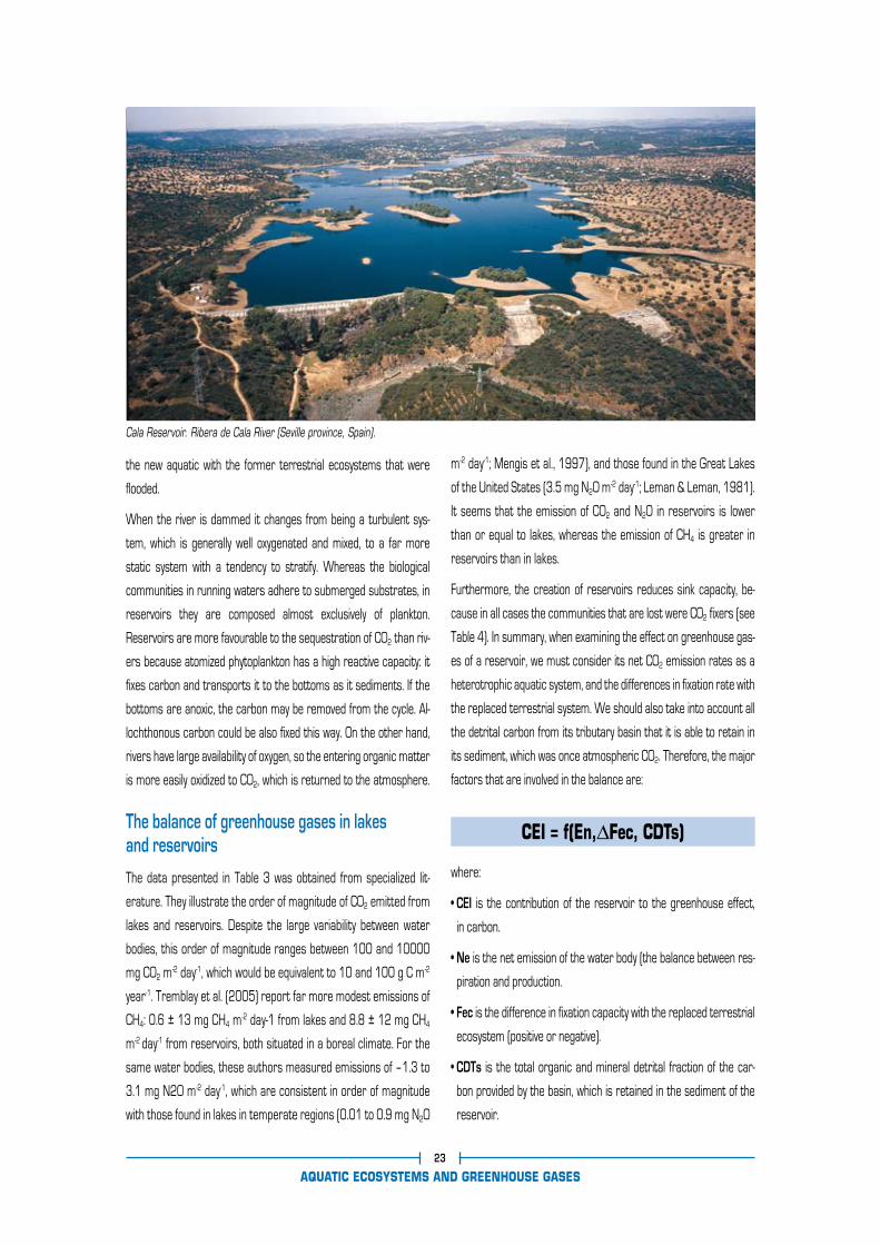
the new aquatic with the former terrestrial ecosystems that were

flooded.

When the river is dammed it changes from being a turbulent sys-

tem, which is generally well oxygenated and mixed, to a far more

static system with a tendency to stratify. Whereas the biological

communities in running waters adhere to submerged substrates, in

reservoirs they are composed almost exclusively of plankton.

Reservoirs are more favourable to the sequestration of CO2 than riv-

ers because atomized phytoplankton has a high reactive capacity: it

fixes carbon and transports it to the bottoms as it sediments. If the

bottoms are anoxic, the carbon may be removed from the cycle. Al-

lochthonous carbon could be also fixed this way. On the other hand,

rivers have large availability of oxygen, so the entering organic matter

is more easily oxidized to CO2, which is returned to the atmosphere.

The balance of greenhouse gases in lakes and reservoirsThe data presented in Table 3 was obtained from specialized lit-

erature. They illustrate the order of magnitude of CO2 emitted from

lakes and reservoirs. Despite the large variability between water

bodies, this order of magnitude ranges between 100 and 10000

mg CO2 m-2 day-1, which would be equivalent to 10 and 100 g C m-2

year-1. Tremblay et al. (2005) report far more modest emissions of

CH4: 0.6 ± 13 mg CH4 m-2 day-1 from lakes and 8.8 ± 12 mg CH4

m-2 day-1 from reservoirs, both situated in a boreal climate. For the

same water bodies, these authors measured emissions of –1.3 to

3.1 mg N2O m-2 day-1, which are consistent in order of magnitude

with those found in lakes in temperate regions (0.01 to 0.9 mg N2O

m-2 day-1; Mengis et al., 1997), and those found in the Great Lakes

of the United States (3.5 mg N2O m-2 day-1; Leman & Leman, 1981).

It seems that the emission of CO2 and N2O in reservoirs is lower

than or equal to lakes, whereas the emission of CH4 is greater in

reservoirs than in lakes.

Furthermore, the creation of reservoirs reduces sink capacity, be-

cause in all cases the communities that are lost were CO2 fixers (see

Table 4). In summary, when examining the effect on greenhouse gas-

es of a reservoir, we must consider its net CO2 emission rates as a

heterotrophic aquatic system, and the differences in fixation rate with

the replaced terrestrial system. We should also take into account all

the detrital carbon from its tributary basin that it is able to retain in

its sediment, which was once atmospheric CO2. Therefore, the major

factors that are involved in the balance are:

CEI = f(En,DFec, CDTs)

where:

• CEI is the contribution of the reservoir to the greenhouse effect,

in carbon.

• Ne is the net emission of the water body (the balance between res-

piration and production.

• Fec is the difference in fixation capacity with the replaced terrestrial

ecosystem (positive or negative).

• CDTs is the total organic and mineral detrital fraction of the car-

bon provided by the basin, which is retained in the sediment of the

reservoir.

Cala Reservoir. Ribera de Cala River (Seville province, Spain).

Table 3. CO2 emission from reservoirs and lakes in different countries.

Type of water bodyMean CO2 emission rate

Hydroelectric reservoir (Duchemin et. al., 1995)

Reservoir in Brazil (Rosa et al., 1999)

Reservoirs and lakes ( Southeastern USA, Therrien et al., 2005)

Reservoirs and lakes (Canada, Tremblay et al., 2005)

Hydroelectric reservoirs in Amazonas (Brazil, Rosa et al., 1997)

Canada

Curuá-Una

Manic ReservoirsManic Reference LakeGouin ReservoirGouin Reference Lake

Reservoirs (n=259)Lakes (n= 31)

Embalses (n=56)Lagos (n=43)

Tucuruí ReservoirSamuel ReservoirXingó ReservoirMiranda ReservoirSegredo ReservoirSerra de Mesa ReservoirTrês Marias ReservoirItaipú Reservoir

500-1.000

134,3

1.170 (6470)1.010 (6405)1.165 (6685)1.700 (6950)

664 (61.091)874 (62.214)

1.508 (61.471)1.013 (61.095)

8.4756.7196.0484.3883.8912.6952.6541.138

49,8-99,5

13,4

116,5100,5116,0169,2

66,13 (6108,7)87 (6220,5)

150,2 (6108,7)100,9 (6220,5)

843,6668,6602,1436,8387,3268,3264,2113,3

(mg CO2 wm-2 day -1) (g C m-2 year -1)

Reservoir and lakes (Canada, Duchemin et al., 1999)

AQUATIC ECOSYSTEMS AND GREENHOUSE GASESAQUATIC ECOSYSTEMS AND GREENHOUSE GASES24 25

Baserca Reservoir. Noguera Ribagorzana River (Lleida province, Spain).

Greenhouse gases according to the type of reservoir

Regarding to greenhouse gases balance, nota all reservoirs behave

have different processes in the same way with regard to the balance

of greenhouse gases. The bahaviour dependings on factors such as

climate, location in the basin, hydromorphological characteristics

and trophic state. Their water management should also be taken into

account.

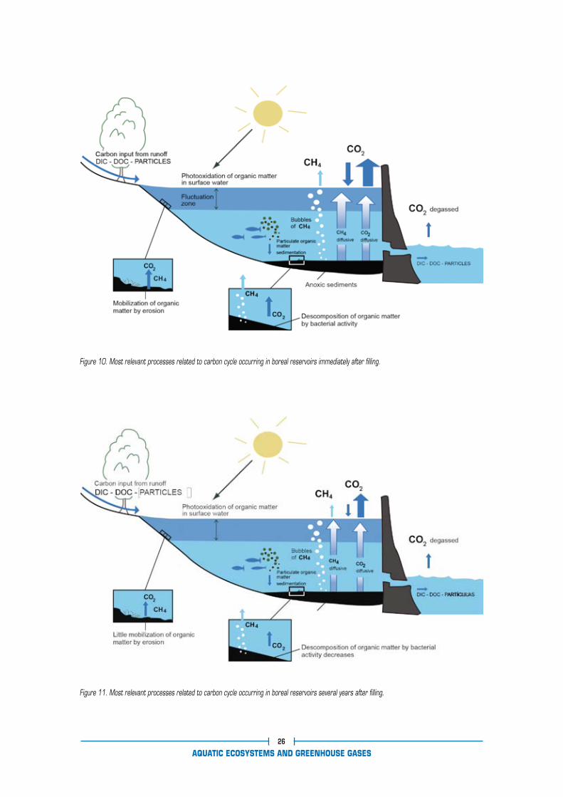
Processes in reservoirs located in boreal zones and semi-arid zones

are similar (Figures 10 and 11). They emit high levels of CO2 and CH4

during the first decade after flooding, then the emission rates are

very low. CO2 emission is always higher than CH4 emission. Tropical

reservoirs have a greater input of particulate organic matter, which

increases the reducing power of the sediments and favours the emis-

sion of CH4 rather than CO2. Additionally, in these reservoirs the net

emissions of greenhouse gases are higher than in boreal and semi-

arid zones. The heterotrophic stage after filling lasts for 10 years

or may even be maintained for ever due to the high loads of organic

matter per unit area covered by water (Figures 12 and 13). All the

carbon involved in these balances belongs to the current carbon cy-

cle, so it does not have the same impact on the environment as the

carbon from fossil fuels. This is must be kept in mind.

Table 4. Mean CO2 fixation rates on both a daily and an annual basis for different land vegetal communities.

Type of community

Mean CO2 fixation rate

(mg CO2 wm-2 day -1) (g C m-2 year -1)

Arid steppe

Unirrigated agricultural land

Irrigated agricultural land

Mediterranean shrubland

Humid shrubland

Mediterranean woodland

Humid woodland

502

804-1.205

1.004-1.406

804-1.004

1.506

1.406

2.511

50

80-120

100-140

80-100

150

140

250

AQUATIC ECOSYSTEMS AND GREENHOUSE GASESAQUATIC ECOSYSTEMS AND GREENHOUSE GASES24 25

Chocón Reservoir. Limay River (Neuquén, Argentina).It supplies the largest hydroelectric plant in Argentina. It has 20,200 Hm3 in capacity and 816 km2 in area.

AQUATIC ECOSYSTEMS AND GREENHOUSE GASESAQUATIC ECOSYSTEMS AND GREENHOUSE GASES26 27

Figure 10. Most relevant processes related to carbon cycle occurring in boreal reservoirs immediately after filling.

Figure 11. Most relevant processes related to carbon cycle occurring in boreal reservoirs several years after filling.

AQUATIC ECOSYSTEMS AND GREENHOUSE GASESAQUATIC ECOSYSTEMS AND GREENHOUSE GASES26 27

Figure 12. Most relevant processes related to carbon cycle occurring in tropical reservoirs immediately after filling.

Figure 13. Most relevant processes related to carbon cycle occurring in tropical reservoirs several years after filling.

AQUATIC ECOSYSTEMS AND GREENHOUSE GASES28

The location of the reservoir in the basin determines the load of al-

lochthonous organic matter that can enter it. Reservoirs located in

the headwaters of rivers also have small catchment areas and in

theory have less carbon to oxidize. However, in highly forested areas

the large biomass input can create peat bogs which emits more CH4

than CO2, i.e. they have a greater potential for greenhouse effect. As

reservoirs occupy lower reaches, there is increasing likelihood of re-

ceiving external inputs of dissolved and particulate organic matter,

not only from natural communities but also from cultural activities.

These inputs increase the heterotrophic metabolism of the reservoir

and its potential for emission of greenhouse gases.

The water regime combined with the volume of the reservoir deter-

mines the rate of water renewal. As the rate decreases it favours

phytoplankton growth and consequently the formation of an au-

totrophic system, which increases CO2 fixation by the stored water.

Regarding morphometry, two extreme scenarios can be defined. On

one hand, the embedded reservoirs with steep slopes and therefore

a low relative area subject to water level fluctuations and on the other

hand, the reservoirs with gentle slopes in which small decreases of

water level expose large areas of land. In the first case, the waves

beating the shore transport the sedimented organic matter to the

water column and then to the bottom, which is a carbon trap if re-

ducing conditions are predominant. In the second case the organic

matter in the shallow areas is recycled in situ, with the consequent

emission of greenhouse gases. However, reservoirs with this kind of

morphology, are more prone to eutrophication.

The trophic status is equivalent to the biogenic capacity of the aquatic

ecosystem and is regulated by the nutrient load (particularly phos-

phorus) received by the water body, which is considered to be the

limiting factor in biological production. Limnologists classify lakes and

reservoirs on a scale ranging from oligotrophic to eutrophic waters,

i.e. from unproductive to highly productive waters. In oligotrophic wa-

ters there is little life, and therefore few biogeochemical changes take

place. Eutrophic waters (i.e. well fed) waters can become extremely

reactive and very dynamic in their physicochemical characteristics,

particularly the parameters related to biological phenomena. In

lakes, the biological community shows varying degrees of diversity.

The maximum degree of complexity includes a number of elements

such as littoral and submerged aquatic vegetation, zoobenthos, fish,

zooplankton and phytoplankton. The trophic level is depends on the

features of the water body, which favours the development of certain

elementstherefore expressed in a greater development of the ele-

ments that are most favoured by the characteristics of the wa- ter

body. Generally, in shallow lakes eutrophication leads to a greater-

Accumulation of different scoured materials in the dam of Sabiñánigo Reservoir (Gállego River, Huesca province, Spain).

AQUATIC ECOSYSTEMS AND GREENHOUSE GASES29

favours the development of submerged macrophytes. In reservoirs,

due to their permanent state of immaturity, the matter and energy

flow mainly through plankton, particularly especially phytoplankton,

and through the heterotrophic bacteria that are found in the plank-

tonit and in the benthos.

Eutrophic reservoirs have high turbidity due to suspended algae, green

water and their chemical features tend to be stratified: high oxygen,

high pH and low phosphorus at the surface; low oxygen, low pH and

higher phosphorus in deep waters. The higher the trophic status of

lakes and reservoirs, the greater the amount of atmospheric CO2 they

fix. However, the final balance depends on other characteristics that

determine the potential to return the fixed carbon to the atmosphere.

Among them, the most important are the oxidation of the sediments

and the alkaline reserve. If the carbon-enriched sediments remain

anoxic, the carbon is immobilized or transformed into CH4, though

this process is efficient only in absence of SH2, which inhibits metha-

Cárdena Reservoir. Cárdena River (Zamora province, Spain).

Negratín Reservoir. Guadiana Menor River (Granada province, Spain).

nogenic activity. On the other hand, if there is enough calcium in the

water, the increases in pH associated with photosynthesis favour the

precipitation of CaCO3, which has a very low solubility. Consequently,

the reservoir model with the greatest capacity to sequester carbon

is the one with deep eutrophic waters that are highly mineralized by

both calcium and sulfates, which are precursors of SH2. Furthermore,

shallow eutrophic reservoirs—particularly if the waters are weakly

mineralized—return the fixed carbon to the atmosphere in the form

of CO2 and/or CH4, and the net balance of the production-respiration-

decomposition cycle tends to be null.

The water management also affects the rate of water removal in the

reservoir, the fluctuations in level and the selection of the depth from

which the outgoing water is taken. The less time the water is retained

in the reservoir, the lower the autotrophic activity, the higher the ten-

dency to emit CO2, and the lower the possibility of retention of carbon

by sedimentation of organic and inorganic matter. Changes in water

level imply changes in depth. When the depth falls, anoxic zones re-

ceive dissolved oxygen more easily and oxidizing conditions can be

established. Some flooded areas may even dry out, with the resulting

oxidation of the stored organic carbon to CO2.

Finally, water is usually released from the deep levels of reservoirs,

where water is rich in dissolved and particulate organic carbon of

detrital origin. This carbon is released into the atmosphere under

AQUATIC ECOSYSTEMS AND GREENHOUSE GASES30

the more oxidizing conditions downstream. CO2, CH4 and N2O may

also be emitted by these deep waters through degasification, as

stated above. Finally, unlike lakes located in basins that are in a

state of hydromorphological balance, reservoirs are condemned to

be filled with sediment. The sediment load transported by the tribu-

tary river is deposited at the bottom of the reservoir, where it buries

both the allochthonous organic sediments and those that are syn-

thesized in the reservoir. These sediments are rarely remobilized,

so the net result is carbon retention. Therefore, the rate of siltation

is the last important factor to take into account in the carbon bal-

ance of stored water bodies.

Mediano Reservoir Cinca River (Huesca province, Spain). Sedimentary de-posit uncovered by the almost complete emptying of the reservoir.

Linsoles reservoir. Ésera River (Huesca province, Spain).

INTRODUCCIÓN22

IV

A CASE STUDY: THE SUSQUEDA RESERVOIR

(TER RIVER, GIRONA)

A CASE STUDY: THE SUSQUEDA RESERVOIR (TER RIVER, GIRONA)32

1. INTRODUCTION

The overall role of reservoirs in the balance of greenhouse gases is

of little importance in Spain because their surface water layer repre-

sents only 0.61% of the total land area. However, as Spain is the Eu-

ropean country with the greatest number and diversity of reservoirs,

the study of the carbon balance in the Susqueda reservoir that is

presented in this publication is of great interest.

Between 2002 and 2003, ENDESA conducted a study of the carbon

balance in the Susqueda Reservoir over an annual cycle. This res-

ervoir is located in the middle stretch of the Ter River between the

Sau and El Pasteral Reservoirs in the province of Girona (Figure 14).

The Susqueda Reservoir is medium-sized, eutrophic and moderately

mineralized. Table 5 summarizes its main characteristics during the

study period.

Figure 14. Location map of the reservoir network including Sau, Susqueda and Pastoral Reservoirs (Ter River, Girona province, Spain).

View of the dam and the two intake towers.

A CASE STUDY: THE SUSQUEDA RESERVOIR (TER RIVER, GIRONA)33

2. THE APPROACH TO THE STUDY

Gas emissions from aquatic systems can be estimated by vari-

ous methods. Canadian scientists have been measuring emis-

sions of greenhouse gases in aquatic systems since 1993,

using floating chambers for gas collection placed on the water

surface. that collect the gases. These Gases are measured

in situ or in the laboratory by infrared chromatography. Of

course, these methods require a large number of measure-

ments in both space and time in order to obtain be repre-

sentative.

Table 5. Hydromorphological and physico-chemical features of the Susqueda Reservoir during the 309 days of the study.

Tabla 5. xxxxxxxxxxxxxxxxxxxxxxxxxxxxxxxxxxxx

Hydromorphological features

Physico-chemical features

April 2002 March 2003

Reservoir water volume at maximum water level (hm3)

Reservoir water volume (hm3)

Maximum operative water level elevation (m a.s.l.)

Incoming water in hm3 during the study

Reservoir water level (m a.s.l.)

Maximum depth (m)

233

86,48

351

376,46

Outgoing water in hm3 during the study 305,73

Thermal characteristics Summer stratification. Permanent deep cold water mass

Electric conductivity (mS/cm) 373-756

Alkalinity (meq/L) 1,76-2,93

Water transparency in m (Secchi disc) 0,6-6,47

pH (und) 7-9

Dissolved oxygen Permanent hypoxia or anoxia in deep water

316,64

56

348,20

>95

215,12

In the project carried out by ENDESA, it was decided to use a “black box”

model, measuring or estimating carbon fluxes at the inflows and out-

flows of the reservoir. This model is based on the assumption that the

incoming amount is equal to the outgoing amount, which includes the

amount of carbon stored in the sediment plus the amount stored in the

body of water due to the increase in volume during the study period.

The inputs are:

• TCin = total carbon in the water flowing into the reservoir from the

Sau Reservoir (measured).

• TCdi = total carbon in the diffuse inflow to the reservoir from the

main basin (estimated).

The outputs are:

• TCout = total carbon of the outgoing water from the reservoir into

the Ter River (measured).

• TCsed = carbon accumulated in the sediment of the reservoir (estimated

from the measurements obtained in the surface layer of sediment).

The air-water exchange of CO2 is :

• CO2 = net exchange of CO2 between the water and the air (calcu-

lated from the difference in concentration of CO2 concentration in

between the water and in the atmosphere).

The amount stored is:

• TCsto = total carbon stored in the water of the reservoir (calculated from

the difference between the initial and final volume of the reservoir in the

study period, multiplied by the carbon concentration of the outflow).

The balance can be expressed as:

TCin+TCdi = TCout

+ TCsed + DTCsto

+ DCO2

A CASE STUDY: THE SUSQUEDA RESERVOIR (TER RIVER, GIRONA)34

The measured or estimated forms of carbon that were measured or

estimated were:

• In the water flowing into and out of the reservoir:

– Dissolved inorganic carbon (DIC) based on alkalinity and pH.

– Organic carbon: dissolved (DOC) and particulate (POC).

• In the sediment traps: Particulate organic carbon (POC) and par-

ticulate inorganic carbon (PIC).

• In the air-water interface: exchange of CO2.

• In the sediment: Particulate organic carbon and particulate inor-

ganic carbon (POC and PIC).

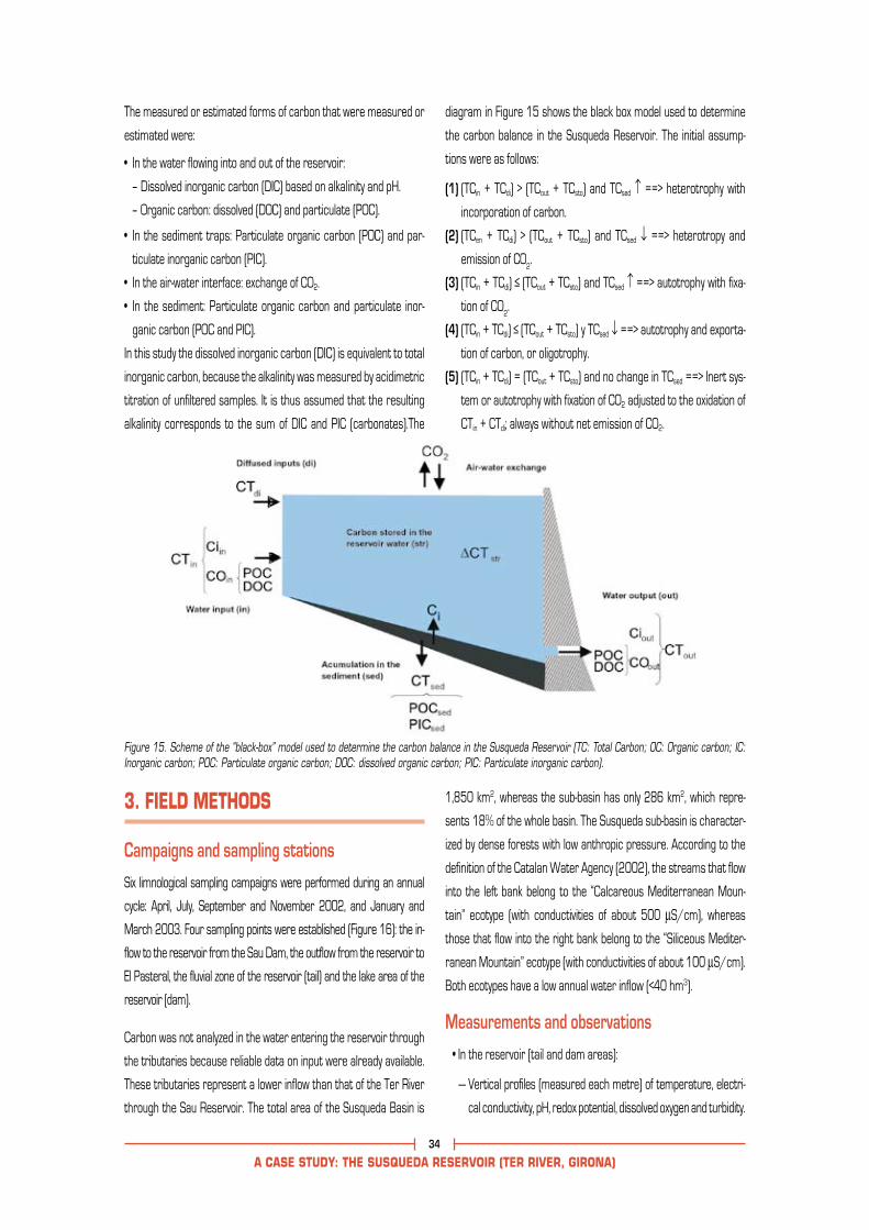
In this study the dissolved inorganic carbon (DIC) is equivalent to total

inorganic carbon, because the alkalinity was measured by acidimetric

titration of unfiltered samples. It is thus assumed that the resulting

alkalinity corresponds to the sum of DIC and PIC (carbonates).The

diagram in Figure 15 shows the black box model used to determine

the carbon balance in the Susqueda Reservoir. The initial assump-

tions were as follows:

(1) (TCin + TCdi) > (TCout + TCsto) and TCsed ↑ ==> heterotrophy with

incorporation of carbon.

(2) (TCen + TCdi) > (TCout + TCsto) and TCsed ↓ ==> heterotropy and

emission of CO2.

(3) (TCin + TCdi) ≤ (TCout + TCsto) and TCsed ↑ ==> autotrophy with fixa-

tion of CO2.

(4) (TCin + TCdi) ≤ (TCout + TCsto) y TCsed ↓ ==> autotrophy and exporta-

tion of carbon, or oligotrophy.

(5) (TCin + TCdi) = (TCout + TCsto) and no change in TCsed ==> Inert sys-

tem or autotrophy with fixation of CO2 adjusted to the oxidation of

CTin + CTdi; always without net emission of CO2.

3. FIELD METHODS

Campaigns and sampling stationsSix limnological sampling campaigns were performed during an annual

cycle: April, July, September and November 2002, and January and

March 2003. Four sampling points were established (Figure 16): the in-

flow to the reservoir from the Sau Dam, the outflow from the reservoir to

El Pasteral, the fluvial zone of the reservoir (tail) and the lake area of the

reservoir (dam).

Carbon was not analyzed in the water entering the reservoir through

the tributaries because reliable data on input were already available.

These tributaries represent a lower inflow than that of the Ter River

through the Sau Reservoir. The total area of the Susqueda Basin is

POCsed

PICsed

Figure 15. Scheme of the “black-box” model used to determine the carbon balance in the Susqueda Reservoir (TC: Total Carbon; OC: Organic carbon; IC: Inorganic carbon; POC: Particulate organic carbon; DOC: dissolved organic carbon; PIC: Particulate inorganic carbon).

1,850 km2, whereas the sub-basin has only 286 km2, which repre-

sents 18% of the whole basin. The Susqueda sub-basin is character-

ized by dense forests with low anthropic pressure. According to the

definition of the Catalan Water Agency (2002), the streams that flow

into the left bank belong to the “Calcareous Mediterranean Moun-

tain” ecotype (with conductivities of about 500 mS/cm), whereas

those that flow into the right bank belong to the “Siliceous Mediter-

ranean Mountain” ecotype (with conductivities of about 100 mS/cm).

Both ecotypes have a low annual water inflow (<40 hm3).

Measurements and observations • In the reservoir (tail and dam areas):

— Vertical profiles (measured each metre) of temperature, electri-

cal conductivity, pH, redox potential, dissolved oxygen and turbidity.

Figure 17. Field work carried out in the Susqueda Reservoir.

A CASE STUDY: THE SUSQUEDA RESERVOIR (TER RIVER, GIRONA)35

— Measurements of the Secchi disc depth.

— Water sampling for analysisto determine of the alkalinity at dif-

ferent water levels: surface, Secchi Disc depth (2.7 SD), thermo-

cline, hypolimnion and bed.

— Water sampling of the sedimentation traps for analysis of the

matter sedimented (particulate organic and inorganic carbon

and undissolved solids) during the time between two consecu-

tive campaigns.

— Extraction of sediment samples at the dam station through a

Phleger Corer sampling unit with a tube 3 cm in diameter and

60 cm long for subsequent dating and determination of the or-

ganic and inorganic carbon content. In an initial campaign, sedi-

ment samples were taken at the tail and dam with an Ekman-type

dredge for a preliminary characterization of sediment (color,

smell, texture, presence of gases, etc.).

• At the inflows and outflows:

— In situ measurements of temperature, conductivity, pH, redox

potential, turbidity and dissolved oxygen in water.

— Water sampling for analysis of alkalinity and organic carbon.

Installation of the sedimentation traps

Two sedimentation traps were placed at each sampling point of the

reservoir (dam and tail): a fixed one to calculate the sedimented mat-

ter throughout the entire study cycle and anone other containing the

matter sedimented between two consecutive campaigns (every two

months). The traps consisted of an opaque PVC tube 1 m long and

9 cm in diameter, closed at the lower end. They were, anchored about

5 m from the bottom, and kept vertical by submerged floats located

about 15 m above the trap and tied to a surface buoy by a line whose

length allowed for the fluctuation in the water level of the reservoir.

Figure 16. Approximate location of sampling points.

4. ANALYTICAL METHODS

Table 6 shows the test methods used on the samples. In the core

collected at the deepest part of the reservoir, the sedimentation

processes were dated using absolute radiometric techniques

(210Pb, 226Ra and 137Cs) and the amount of organic and inorganic

carbon accumulated throughout the history of the reservoir was

measured.

A CASE STUDY: THE SUSQUEDA RESERVOIR (TER RIVER, GIRONA)36

A CASE STUDY: THE SUSQUEDA RESERVOIR (TER RIVER, GIRONA)37

Table 6. Assay methods used to analyze the samples taken in the Susqueda reservoir.

Samples

Water

Alkalinity Acidimetry. NAQUADAT 10101 method.

Total organic carbon Catalytic oxidation. Detection with IR analyzer. EPA 9069 method.

Dissolved organic carbonCatalytic oxidation. Detection with IR analyze after filtering through glass fibre filters. EPA 9060 method.

Sedimented matter

Sedimented matter

Total Carbon

Particulate organic carbon

Total inorganic carbon

Carbono inorgánico total

Filtration with a GF/C filter. Dry residue is oxidized with oxygen and cobalt oxide as catalyzer. CO2 measured with IR analyzer.

Filtration with a GF/C filter. The dry residue is previously treated with HCl to remove organic carbon from it. DHROMANN 190 analyzer equipped with a module for solid matter (MOD. 183).

Oxidation.

Acid attack.

Parameter Method

Table 7. Dissolved inorganic (DIC), organic (DOC) and particulate organic (POC) carbon in the incoming and outcoming water of the Susqueda Reservoir.

Carbon

Incoming

DIC 34,94 32,90 33,41 36,20 36,13 37,14 35,08

DOC 3,59 3,67 3,40 2,93 3,42 4,28 3,48

POC 0,85 0,30 0,16 0,39 0,73 0,66 0,47

DIC 34,68 31,45 30,89 29,95 31,61 33,74 31,90

DOC 3,18 4,07 4,90 3,44 3,33 3,56 3,83

POC 0,72 1,06 0,43 0,18 0,77 0,70 0,64

Outgoing

Apr 29 Jul 22 Sep 10 Nov 14 Jan 14 Mar 4 Annual weighted mean

5. RESULTS

Carbon in the inflowing water from Sau (CTin) and the outflow from the reservoir (CTout)All forms of carbon measured at the inflow and outflow of the

reservoir showed little variation during the study period. The tem-

poral pattern of POC is very similar to that described for the sedi-

mentation traps (Table 7). The sum of the annual weighted averages

(for the time between campaigns) of all forms of carbon in the in-

flowing and outflowing water reveals that during the course of study

the average carbon concentration in water from Sau (inflowing wa-

ter: 39.04 mg/L) was greater than that in the water flowing out to

El Pasteral (outflow water: 36.36 mg/L).

A CASE STUDY: THE SUSQUEDA RESERVOIR (TER RIVER, GIRONA)36

A CASE STUDY: THE SUSQUEDA RESERVOIR (TER RIVER, GIRONA)37

Carbon from the sub-basin of the reservoir (TCdi)

During the study period there was an increase of 128.67 hm3 in the

volume of water stored, 70.73 coming from Sau and 57.94 from the

Susqueda sub-basin. The carbon load of the sub-basin was estimated

from existing data for the Riera Major creek (Butturini, 1997; Martí

i Sabaté, 1996), whose water inflow is approximately 50% of the an-

nual total, and assuming that similar carbon concentrations in all the

tributaries. According to the studies cited, the average concentra-

tion in this creek is 18.1 mgC/L, so the total load is estimated to be

1048.7 t .

Carbon incorporated in the water (TCsto)

The carbon incorporated in the water of the reservoir was calculated

as the difference between the final and initial volume (128.67 hm3)

multiplied by the average outflow concentration (36.36 mg/L). We

estimated 4678 t of carbon by this procedure.

Carbon accumulated in the sedimentation traps

The annual sedimentation of organic carbon (POC) and inorganic

carbon (PIC) was calculated from the sediment that accumulated

in the traps during the 309 days of the study (Figure 18). The

rate of sedimentation was 4 times greater at the tail of the res-

Figure 18. Particulate organic (POC) and inorganic (PIC) carbon sediment-ed in the traps during the study.

Figure 19. Evolution of the daily sedimentation rate of organic (POC) and inorganic (PIC) carbon in the sedimentation traps installed at the tail and the dam of the Susqueda Reservoir. The content of the traps was removed every two months.

ervoir than in the dam area; furthermore, in both zones the rate

of sedimentation of POC was greater than that of PIC. From the

data of the traps, whose content was removed every two months,

we determined the evolution of the carbon sedimentation rate,

which followed the pattern of water inflow from Sau in the tail

area and the pattern of thermal stratification of the reservoir in

the dam area.

Table 9. Organic and inorganic carbon sedimented during one year on the dam area of the Susqueda Reservoir.

Sedimented carbon on the dam area

Carbon sedimentation rate (bi-monthly traps) (g C cm2 year-1) 0,0211

0,0151

0,0138

0,0874Carbon sedimentation rate (monthly trap) (g C cm2 year-1)

Carbon

organic inorganic

A CASE STUDY: THE SUSQUEDA RESERVOIR (TER RIVER, GIRONA)38

A CASE STUDY: THE SUSQUEDA RESERVOIR (TER RIVER, GIRONA)39

thermal stability (vertical mixing of the water column) but higher

hydrodynamic stability (lower water flow through the reservoir). In

the tail area, under far more complex hydrodynamic conditions due

to the influence of incoming water, the sedimentation rate should

be even more correlated to the incoming flow pulses. The larger in-

coming flows in January increased the sediment loads in the traps

placed in the tail area.

As the Susqueda reservoir has a narrow section and the water flow-

ing into it from the bottom of the Sau Reservoir is normally cold, tur-

bidity currents are quite often formed. Indeed, in February a mass

of turbid water (15 NTU) circulating at depth and generated by an

increase in the turbine discharge from the Sau Reservoir was de-

tected in the tail area.

The total carbon settled in one year (Table 9), calculated from the

data of traps placed in the dam area, will be compared later with the

data of carbon accumulation in the sediment at the bottom of the

reservoir, collected by core sampler.

Figure 19 and Table 8 show the low sedimentation levels during

the months of thermal stratification. When the mixing of the res-

ervoir starts, the sedimentation rate increases in the tail area,

which loses its vertical stability first, and then rises sharply in the

dam area. In February the rate of sedimentation in the tail area

increased significantly again. This evolution seems contradictory

because the highest rates of sedimentation are associated with

the times of vertical mixing of the water column. This shows the im-

portance of the hydrodynamic behaviour of the water mass stored

at each moment. In the dam area, the highest rate of sedimenta-

tion occurred in December, with low incoming and outgoing flows

both before and during the sampling (Table 8); when there is lower

Carbon (g C m-2 day-1)

DamPOC 0,38 0,21 0,15 2,14 –

PIC 0,26 0,09 0,07 1,45 –

POC – 0,29 0,81 0,34 1,79

PIC – 0,17 0,46 0,21 1,24Tail

inicial date

Final date

Nov 14 Jan 14

Mar 4Jan 14

Sep 10

Nov 14

Jul 22

Sep 10

Apr 29

Jul 22

Incoming flor Vol. (m3/s) 20,16 12,15 11,89 6,73 17,73

Incoming Vol. (hm3) 148,09 52,50 66,81 35,52 73,55

Outgoing Vol. (hm3) 67,55 49,36 74,10 47,41 67,31

Table 8. Daily rate of organic (POC) and inorganic carbon deposition in the sedimentation traps installed in the tail and the dam of the Susqueda Reservoir.

A CASE STUDY: THE SUSQUEDA RESERVOIR (TER RIVER, GIRONA)38

A CASE STUDY: THE SUSQUEDA RESERVOIR (TER RIVER, GIRONA)39

Table 10. Sediment age at different depths in the Susqueda Reservoir, determined by absolute radiometric dating, together with sedimentation rate, carbon content and carbon accumulation rate in the sediments of each time interval.

Depth (cm) Year

Sedimentation rate

(cm year-1) (g C cm-2 year-1)

Carbon content

organic

(g C cm-2 year-1)(% C dw)

inorganic

Carbon accumulation rate

organic inorganic

1,3

3,5

5,5

7,5

9,5

11,5

13,5

2002

2000

1998

1996

1994

1991

1987

1,17

1,06

1,00

1,00

0,80

0,57

0,50

0,29

0,27

0,28

0,26

0,19

0,23

0,19

1,85

1,61

1,55

1,80

1,43

1,55

1,38

0,0209

0,0186

0,0190

0,0182

0,0131

0,0152

0,0120

0,0054

0,0042

0,0043

0,0047

0,0027

0,0036

0,0026

7,20

6,90

6,80

7,00

6,91

6,60

6,30

Carbon incorporated in the sediment (Ctsed) The content of the core sample obtained in the dam area was taken

as an estimation of the carbon incorporated in the sediment during

an interval in the life of the Susqueda Reservoir. Table 10 shows the

results of the core dating, and the carbon content of the different

sections of the sediment column. The table also indicates the cor-

respondence between the depth of the sediment and the year of

deposition, and the sedimentation rate calculated for each section.

Table 11. Particulate organic (POC), inorganic (PIC) and total carbon accumulation rate in the Susqueda Reservoir.

Inorganic carbon

Total carbon (t C year-1)

POC sedimentation rate

Total carbon (tC in 309 days)

Dam (core)

0,0209

149,2

0,0054

126,3

Tail (estimated)

0,0847

606,4 755,6

0,0220

513,4 639,6

Reservoir

The average sedimentation rate in the Susqueda Reservoir amounted

towas 0.84 cm/year, with a maximum of 1.17 cm/year in the most

recent layer (surface) and 0.50 cm/yr in the oldest layer (deep). In the

Sau Reservoir, using a 46.5 cm core, Armengol et al. (1984) estimated

the sedimentation rate by , correlating the apatite phosphorus concen-

tration with the monthly inflow of water into the reservoir. The resulting

sedimentation rates were 1.5 cm/yr in dry periods and 3-4.5 cm/year

in rainy periods.

Reservoirs act as decanters of sediment, so the rate of sedimenta-

tion was expected to be lower in the Susqueda Reservoir than in Sau,

which is located upstream. Since the most recent sediment sections

have higher organic and inorganic carbon content, we considered

the carbon accumulation rate of the uppermost layer of sediment,

which includes the last two years. Furthermore, data from the an-

nual traps were used to correct the extrapolation of the core result

to the whole reservoir, considering that, according to the results,

the sedimentation rate is four times higher in the tail area than in

the dam area.

The total volume of the sediment layer was determined as the prod-

uct of the sediment rate by the area of the reservoir bed potentially

occupied by sediment, i.e. that with a slope of less than 14% (Hakan-

son, 1981). By analyzing detailed maps of the dam area (1:10,000)

and the tail area (1:50,000) before the flooding of the reservoir, we

obtained a sediment area of 113.66 ha. The accumulation rates at

the tail (estimated) and dam (the core sample) were allocated to 50%

Net CO2 exchange (t C in 309 days)

Tail

11,0

Dam

74,9

Reservoir

85,9 (emission)

Table 13. CO2 exchange during different time intervals in the Susqueda Reservoir.

CO2 exchange Apr 29 Nov 14 Jul 22 Jan 14 Sep 10 Mar 4

Tail(mg C m-2 day -1)

(mmol C m-2 day -1)

-80,9

-6.742

59,8

4.983

-78,3

-6,527

106,7

8.890

-21,2

-1.766

173,5

14.461

Dam

Surface

(mg C m-2 day -1)

(mmol C m-2 day -1)

(ha)

-104,5

-8,711

317

81,2

6.768

434

8,5

711

432

512,5

42.708

430

-26,5

-2.211

438

222,0

18.503

451

of the total sediment area in accordance with the apparent hydro-

dynamic organization of the reservoir (Table 11). The accumulation

rates obtained by the core are slightly lower for organic carbon and

higher for inorganic carbon than those obtained from sediment traps

in the dam area (Table 12).

The data obtained from the core seem the best suited to perform

the final carbon balance, as they are an estimate of the carbon that

has actually accumulated in the sediment. On the other hand, the

data from the sediment traps are an estimate of the carbon that

could potentially end up in the sediment but may still be subject to

a variety of biological and physico-chemical processes. The estimate

could also be affected by situations of resuspension or accumulation

of carbonated matter through physical processes, according to the

hydrodynamics of the water body at any given time.

A CASE STUDY: THE SUSQUEDA RESERVOIR (TER RIVER, GIRONA)40

A CASE STUDY: THE SUSQUEDA RESERVOIR (TER RIVER, GIRONA)41

Carbon incorporation to sediment in the dam

Accumulation rate in superficial sediment (core)

Carbon sedimentation rate (yearly trap)

Carbon

organic

0,0209

0,0151

inorganic

0,0054

0,0874

Table 12. Comparison between the rates of carbon incorporation to the sediments estimated by sedimentation traps and cores.

Exchange of CO2 between water and airThe diffusive flux of CO2 from the water into the atmosphere, or vice

versa, was calculated according to the following expression:

Flow = DG x (C - CO2 )a - (C - CO2)W

where:

• DG is the molecular diffusivity of CO2 in water, corrected for water

temperature (Broecker & Peng, 1982).

• [C-CO2]a is the carbon concentration (weight/volume) of CO2 in the

air, calculated as a function of atmospheric pressure at the altitude

of the reservoir, the air temperature and the amount of CO2 in the air;

• [C-CO2]w is the carbon concentration (weight/volume) of CO2 in the

layer corresponding to the epilimnion in summer (between 1.5 and

5 m from the surface) or the uppermost layer in winter (top 5-6 m).

It was calculated from the dissolved inorganic carbon data obtained

through the data on alkalinity, water temperature and pH (Stumm

& Morgan, 1996).

• Z is the boundary water layer, which was estimated based on the

average wind speed during sampling, from the calculation expres-

sionsformulae of Broecker and Peng (1982), applying a polynomial

relationship between the two variables.

The meteorological data (air temperature, atmospheric pressure

and wind speed) for calculating the exchange of CO2 between wa-

ter and air was taken at the meteorological station of the University

of Barcelona located at the Sau Yacht Club (coordinates: 41º 58’

32.15’’ N; 2º 23’ 54.44’’ E).

The evolution of the exchange of CO2 between water and air shows

that in the most productive months there is greater incorporation of

Z

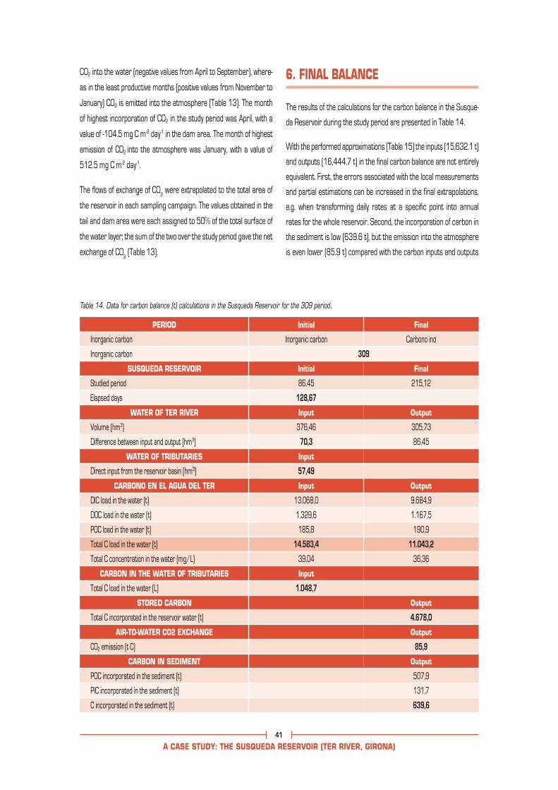
A CASE STUDY: THE SUSQUEDA RESERVOIR (TER RIVER, GIRONA)40

A CASE STUDY: THE SUSQUEDA RESERVOIR (TER RIVER, GIRONA)41

PERIOD

Inorganic carbon

Inorganic carbon

SUSQUEDA RESERVOIR

Studied period

Elapsed days

WATER OF TER RIVER

Volume (hm3)

Difference between input and output (hm3)

WATER OF TRIBUTARIES

Direct input from the reservoir basin (hm3)

CARBONO EN EL AGUA DEL TER

DIC load in the water (t)

DOC load in the water (t)

POC load in the water (t)

Total C load in the water (t)

Total C concentration in the water (mg/L)

CARBON IN THE WATER OF TRIBUTARIES

Total C load in the water (L)

STORED CARBON

Total C incorporated in the reservoir water (t)

AIR-TO-WATER CO2 EXCHANGE

CO2 emission (t C)

CARBON IN SEDIMENT

POC incorporated in the sediment (t)

PIC incorporated in the sediment (t)

C incorporated in the sediment (t)

Initial

Inorganic carbon

309

Initial

86,45

128,67

Input

376,46

70,3

Input

57,49

Input

13.068,0

1.329,6

185,8

14.583,4

39,04

Input

1.048,7

Final

Carbono ino

Final

215,12

Output

305,73

86,45

Output

9.684,9

1.167,5

190,9

11.043,2

36,36

Output

4.678,0

Output

85,9

Output

507,9

131,7

639,6

Table 14. Data for carbon balance (t) calculations in the Susqueda Reservoir for the 309 period.

CO2 into the water (negative values from April to September), where-

as in the least productive months (positive values from November to

January) CO2 is emitted into the atmosphere (Table 13). The month

of highest incorporation of CO2 in the study period was April, with a

value of -104.5 mg C m-2 day-1 in the dam area. The month of highest

emission of CO2 into the atmosphere was January, with a value of

512.5 mg C m-2 day-1.

The flows of exchange of CO2 were extrapolated to the total area of

the reservoir in each sampling campaign. The values obtained in the

tail and dam area were each assigned to 50% of the total surface of

the water layer; the sum of the two over the study period gave the net

exchange of CO2 (Table 13).

6. FINAL BALANCE

The results of the calculations for the carbon balance in the Susque-

da Reservoir during the study period are presented in Table 14.

With the performed approximations (Table 15) the inputs (15,632.1 t)

and outputs (16,444.7 t) in the final carbon balance are not entirely

equivalent. First, the errors associated with the local measurements

and partial estimations can be increased in the final extrapolations,

e.g. when transforming daily rates at a specific point into annual

rates for the whole reservoir. Second, the incorporation of carbon in

the sediment is low (639.6 t), but the emission into the atmosphere

is even lower (85.9 t) compared with the carbon inputs and outputs

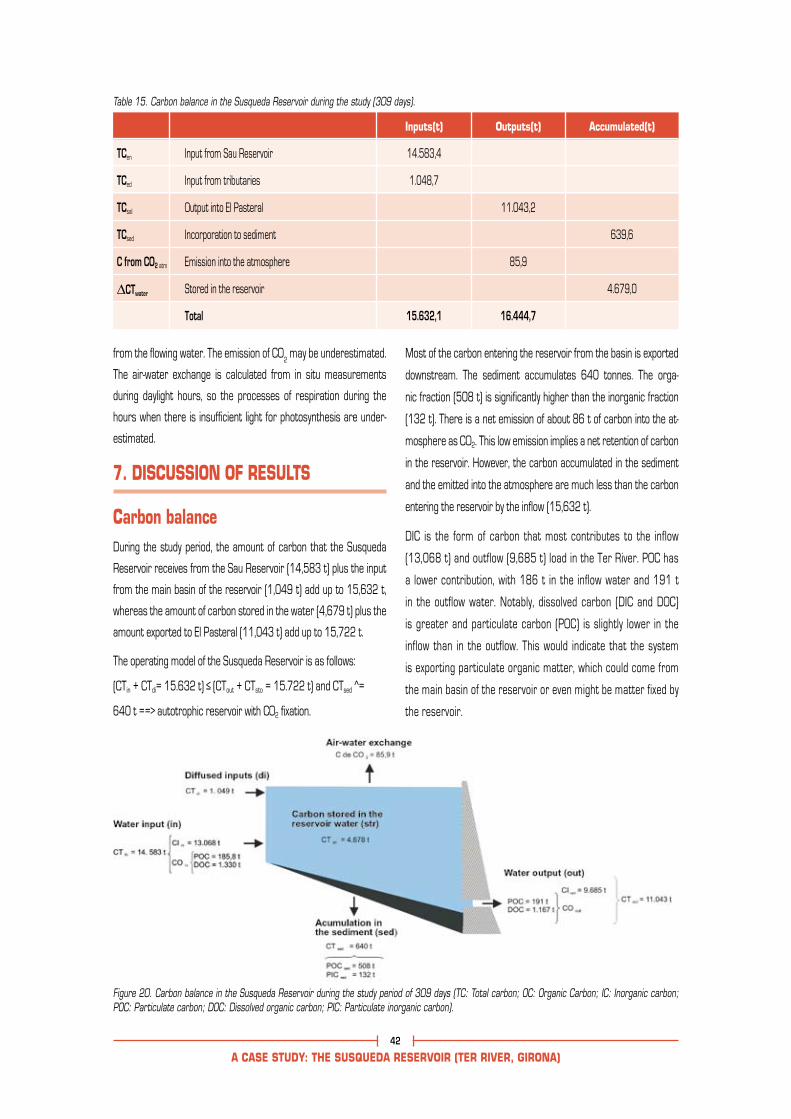
from the flowing water. The emission of CO2 may be underestimated.

The air-water exchange is calculated from in situ measurements

during daylight hours, so the processes of respiration during the

hours when there is insufficient light for photosynthesis are under-

estimated.

7. DISCUSSION OF RESULTS

Carbon balanceDuring the study period, the amount of carbon that the Susqueda

Reservoir receives from the Sau Reservoir (14,583 t) plus the input

from the main basin of the reservoir (1,049 t) add up to 15,632 t,

whereas the amount of carbon stored in the water (4,679 t) plus the

amount exported to El Pasteral (11,043 t) add up to 15,722 t.

The operating model of the Susqueda Reservoir is as follows:

(CTin + CTdi= 15.632 t) ≤ (CTout + CTsto = 15.722 t) and CTsed ^=

640 t ==> autotrophic reservoir with CO2 fixation.

Most of the carbon entering the reservoir from the basin is exported

downstream. The sediment accumulates 640 tonnes. The orga-

nic fraction (508 t) is significantly higher than the inorganic fraction

(132 t). There is a net emission of about 86 t of carbon into the at-

mosphere as CO2. This low emission implies a net retention of carbon

in the reservoir. However, the carbon accumulated in the sediment

and the emitted into the atmosphere are much less than the carbon

entering the reservoir by the inflow (15,632 t).

DIC is the form of carbon that most contributes to the inflow

(13,068 t) and outflow (9,685 t) load in the Ter River. POC has

a lower contribution, with 186 t in the inflow water and 191 t

in the outflow water. Notably, dissolved carbon (DIC and DOC)

is greater and particulate carbon (POC) is slightly lower in the

inflow than in the outflow. This would indicate that the system

is exporting particulate organic matter, which could come from

the main basin of the reservoir or even might be matter fixed by

the reservoir.

A CASE STUDY: THE SUSQUEDA RESERVOIR (TER RIVER, GIRONA)42

A CASE STUDY: THE SUSQUEDA RESERVOIR (TER RIVER, GIRONA)43

Table 15. Carbon balance in the Susqueda Reservoir during the study (309 days).

Total 15.632,1 16.444,7

TCen

TCed

TCsal

TCsed

C from CO2 atm

DCTwater

Input from Sau Reservoir

Input from tributaries

Output into El Pasteral

Incorporation to sediment

Emission into the atmosphere

Stored in the reservoir

Inputs(t)

14.583,4

1.048,7

Outputs(t)

11.043,2

85,9

Accumulated(t)

639,6

4.679,0

Figure 20. Carbon balance in the Susqueda Reservoir during the study period of 309 days (TC: Total carbon; OC: Organic Carbon; IC: Inorganic carbon; POC: Particulate carbon; DOC: Dissolved organic carbon; PIC: Particulate inorganic carbon).

A CASE STUDY: THE SUSQUEDA RESERVOIR (TER RIVER, GIRONA)42

A CASE STUDY: THE SUSQUEDA RESERVOIR (TER RIVER, GIRONA)43

Emission of CO2 into the atmosphereThe rate of carbon emitted into the atmosphere as CO2 (86 t in the

study period) for the Susqueda Reservoir, expressed as a rate, gives

the figuresis shown in Table 16.

ever, the Susqueda Reservoir retains carbon in the sediment, and

its amount (665 g/m2.year) is far higher than that of the replaced

Mediterranean woodlands and shrublands. (between 140 and 80

g/m2.year; Table 4). Therefore, the dam has significantly increased

the carbon sink capacity of the occupied land.

Overall, the contribution of the Susqueda Reservoir to the green-

house effect is as follows (values rounded to unity):

• Net emission (NE) of the water body = +102 t/year

• Difference between the maximum fixation capacity in the reservoir

and in the replaced terrestrial ecosystem (EcF) = - 597 t / year

• Carbon retained in the sediment coming from the basin

(CRs) = -756 t/year.

It can be deduced from the above data that the Susqueda Reservoir:

a) Emits some carbon as CO2 into the atmosphere.

b) Retains in the sediment some of the carbon incoming from its

own basin and from the Sau Reservoir (the fixed amount is about

7.5 times greater than the amount emitted into the atmosphere).

c) Fixes more carbon (almost 5 times) than could be fixed by the origi-

nal Mediterranean terrestrial ecosystem before flooding.

With the data obtained, we conclude that the Susqueda Reservoir

acts as a net carbon sink in absolute terms in comparison with the

terrestrial system that it replaced.

Mean CO2 emission rate

Susqueda dam

Tail area in the Susqueda Reservoir

mg CO2 m-2 day-1

398

48

g C m-2 year-1

39,6

4,9

Table16. Rate of CO2 emission into the atmosphere during the study.

Fixation of carbon in the sedimentsThe total carbon retained in sediment is about 640 t in the

309 studied days; i.e. 756 t per year. This accounts for 665

g/m2.year in the 113.66 ha of the reservoir bed..The calculated

fixation rate of dry organic matter in the seston (about 1663

g/m2.year), it is well above the normal range of sedimentation in

lakes (60 to 200 g/m2.year).

Contribution of the reservoir to the greenhouse effectAAt the gas exchange level, the contribution of CO2 emission from

the Susqueda Reservoir to the greenhouse effect is modest. Moreo-

ver, we must keep in mind that this emission forms part of the cur-

rent carbon cycle, i.e. of the ecosystem respiration in the basin. How-

INTRODUCCIÓN29

V

SOME IMPORTANT FINAL QUESTIONS

IMPORTANT FINAL QUESTIONS45

Between 1993 and 1999, comparative studies of emissions of

greenhouse gases in boreal reservoirs (Finland, Canada) and humid

tropics (French Guiana, Brazil) were carried out. Based on the results

of these studies, and also on those obtained in the Susqueda Reser-

voir, we will try to answer some frequently debated questions about

the role of reservoirs in climate change:

Is it true that reservoirs emit more greenhouse gases than the

natural ecosystems they replace?

In boreal climates forests play a limited role as carbon sinks. Carbon

is emitted during forest fires and after carbon leaching from soils and

forest cover to the watercourses and water bodies, where carbon

compounds are broken down and emitted into the atmosphere. Fur-

thermore, boreal soils fix little carbon.

IIn humid tropical climates, forests may be even more limited sinks

than in boreal climates, since the carbon is rapidly recycled and re-

used by the dense biomass. In these environments, seasonal rains

can flood large areas of forest for long periods (up to 6 months) to a

great depth (2-18 m), so these areas act as tropical reservoirs with

regard to CH4 emission.

The creation of a dam does not reduce the carbon stock in a basin,

but stores it in sediments, where is in a more sealed and stable form

than in forest soils. A biased way of explaining the balance of green-

house gases from reservoirs is to ignore the emissions of ecosys-

tems before the flooding of the valleys. Unfortunately, this type of ap-

proach is still used widely, but it seems clear the inaccuracy of carbon

balance analyses that only consider gross emissions from reservoirs

and not those from the replaced terrestrial ecosystems.

Is it true that reservoirs produce more emissions than natural

lakes and rivers?

In boreal climates emissions of CO2 and CH4 from natural lakes are

similar to those of reservoirs after the initial maturation stage as-

sociated with the flooding of the valleys, which usually takes 6-10

years. In this initial phase, the emissions from reservoirs may be

higher due to the decomposition of the more degradable organic

matter (dead leaves, humus, etc.) covered by the waters. Hence

the importance of taking into account the maturation state of the

reservoirs in greenhouse gas emission studies. In humid tropical

climates methane emissions from rivers and floodplains are similar

to those of reservoirs.

With our current knowledge, what can be said about the net emis-

sions from reservoirs?

There is considerable variability in results depending on several factors.

(trophic characteristics of the reservoir, persistence of thermal strati-

fication, water residence time, surface water layer, basin morphology,

degree of anoxia, etc.). However, in general it can be concluded that

for medium-sized boreal hydroelectric reservoirs (63 km2/TWh) the

emission factor of greenhouse gases per unit of energy produced is

about 11 kt CO2 equivalent/TWh (Gagnon, 2002). This accounts for

1% of the equivalent emissions of a coal power plant and 3% of a

natural gas power plant. The Susqueda Reservoir, with 24 km2/Twh,

only has an emission factor of 2 kt CO2 equivalent/Twh.

In the case of tropical reservoirs, for a comparable surface water

layer the net emission can be up to 10% of that of a coal power plant.

In extreme cases of large, permanently anoxic reservoirs with meth-

ane production, the net emission per unit of energy produced may

be similar to the emission of a coal power plant. Finally, it should be

recalled that all the carbon processed by reservoirs belongs to cur-

rent biogeochemical cycles, in which reservoirs are merely compart-

ments. The role of this carbon emission in the atmospheric balance

related to climate change is not comparable to that resulting from

the use of fossil fuels.

BIBLIOGRAPHY47

BIBLIOGRAPHY

• Agència Catalana de l’Aigua (2002). Regionalització del sistema

fluvial a les Conques Internes de Catalunya. Departament de Medi

Ambient, Generalitat de Catalunya. 92 pp.

• Armengol, J., Crespo, M. & Morguí, J.P. (1984). Phosphorus com-

pounds in the sediment of the Sau reservoir (Barcelona, NE Spain)

throughout its twenty-year existence. Verh. Internat. Verein. Limnol.,

22: 1536-1540.

• Broecker, W.S. & Peng, T.H. (1982). Tracers in the sea. Lamont-

Doherty Geological Observatory. New York. 690 pp.

• Butturini, A. (1997). Contribution of the boundary zones on nutrient

dynamics in a stream with Mediterranean regime. Tesis doctoral.

Departament d’Ecologia, Universitat de Barcelona.

• Duchemin, E., Lucotte, M. & Canuel, R. (1995). Production of the

greenhouse gases CH4 and CO2 by hydroelectric reservoirs of the

Boreal region. Global Biogeochemical Cycles, 9(4): 529-540.

• Duchemin, E., Canuel, R., Ferland, P. & Lucotte, M. (1999). Étude sur

la production et l’émission de gaz à effet de serre par les réservoirs

hydroélectriques de l’entreprise et de lacs naturels (Volet 2), Univer-

sité du Québec a Montreal. 47 pp.

• Gagnon, L. (2002). The International Rivers Network Statement on

GHG emissions from reservoirs, a use of misleading science. Inter-

national Hydropower Association. Sutton (UK). 9 pp.

• Hakanson, L. (1981). A manual of lake morphometry. Springer-

Verlag. Berlin. 78 pp.

• Lean, J. (2004). Solar Irradiance Reconstruction. IGBP PAGES/ World

Data Center for paleoclimatology. Data Contributión Series 2004-35.

NOAA/NGDC Paleoclimatology Program, Boulder (CO). USA.

• Leman, E. & Leman, D. (1981). Nitrous oxide concentrations in fresh

waters of the Great Lakes basin. Limnol. Oceanogr., 26: 867-879.

• Martí, E. & Sabater, F. (1996). High variability in temporal and

spatial nutrient retention in Mediterranean streams. Ecology, 77:

854-869.

• Mengis, M., Gachter, R. & Wehrli, B. (1997). Sources and Sinks of

nitrous oxide (N2O) in deep lokes. Bigeochemistry, 38: 281-301.

• Rosa, L.P., Sikar, B.M., Sikar, E.M., & Santos, M.A. (1997). A model

for CH4 and CO

2 emission mean life in reservoir based on data from

an Amazonian hydroplan. In: Hydropower plants and greenhouse

gas emissions, Rosa, L.P. & Santos, M.A. (eds.). COPPE.

• Rosa, L.P., Matvienko, B., Santos, M.A. & Sikar, E. (1999). Relatório

Eletrobrás/Fundaçao Coppetec. Inventário das emissoes de gases de

effeito estufa derivadas de hidrelétricas. COPPE report to Eletrobras.

• Stumm, W. & Morgan, J.J. (1996). Aquatic Chemistry. Chemical equi-

libria in natural waters. 3rd Edition. John Willey & Sons Inc, N.Y.

• Therrien, J., Tremblay, A. & Jacques, R. (2005). Emissions from

Semiarid Reservoirs and Natural Aquatic Ecosystems. In: Tremblay,

A., Varfalvy, L., Roehm, C. & Garneau, M. (2005). Greenhouse Gas

Emissions: Fluxes and Processes, Hydroelectric Reservoirs and

natural Environments. Environmental Science Series. Springer. New

York. 233-250 pp.

• Tremblay, A. Therrien, J. Hamlin, B. Wichmann, E. & LeDrew, L.

(2005). GHG Emissions from Boreal Reservoirs and Natural Aquat-

ic Ecosystems. In: Tremblay, A., Varfalvy, L., Roehm, C. & Garneau, M.

(2005). Greenhouse Gas Emissions: Fluxes and Processes, Hydroe-

lectric Reservoirs and natural Environments. Environmental Science

Series. Springer. New York. 209-231 pp.

• Tremblay, A., Varfalvy, L., Roehm, C. & Garneau, M. (2005). Green-

house Gas Emissions: Fluxes and Processes, Hydroelectric Res-

ervoirs and natural Environ ments. Environmental Science Series.

Springer. New York. 732 pp.

INTRODUCCIÓN11

EDITORIAL COORDINATION:

Environment and Sustainable Development Department (ENDESA)

DESIGN AND PRINTING:

OFF-7 S.A.

PHOTOGRAPHY:

ENDESA

Printed in November 2008

Legal deposit in Spain L-1133-08

The reproduction in whole or in part of texts and images that appear in this publication is prohibited.

INTRODUCCIÓN10

Environment and Sustainable Development Department (ENDESA)