reservoir performance of fluid systems with widely...

Reservoir Performance of Fluid Systems with

Widely Varying Composition (GOR)

A Simulation Approach

M. Sc. Thesis

Singh Kameshwar

December 1997

ii

Declaration

I hereby declare that this Master of Science thesis has been performed in accordance to

the regulations at the Norwegian University of Science and Technology, Trondheim,

Norway.

Trondheim, December 15, 1997

( Singh Kameshwar )

iii

Preface

This thesis is submitted to the Department of Petroleum Engineering and Applied

Geophysics at the Norwegian University of Science and Technology, Trondheim, in

candidacy for the degree of Master of Science in Petroleum Engineering.

Trondheim, December 15, 1997

( Singh Kameshwar )

iv

Acknowledgement

I sincerely thank to my supervisor, Professor Curtis H. Whitson, for his excellent

guidance, invaluable suggestions and comments throughout the whole work.

I would like to acknowledge NORAD for providing me an opportunity to study in

Norway.

I would also like to thank Øivind Fevang and other colleagues for their technical support

during the thesis work.

Many thanks to the staff of the Department of Petroleum Engineering and Applied

Geophysics, NTNU, especially to Kathy Herje, for the assistance and support rendered to

me.

v

Abstract

Reservoir performance depends on many factors such as drive mechanism, reservoir

rock, and fluid properties. For depletion drive reservoirs, the principal drive mechanism

is the expansion of the oil and gas initially in place. Main factors in depletion drive

reservoirs are total cumulative compressibility, determined mostly by composition

(GOR), saturation pressure and PVT properties, and relative permeability. In this work,

the effect of initial composition (GOR) on recovery, plateau production rate, plateau

production period, and decline constant has been investigated.

In order to analyze the effect of composition (GOR), near critical reservoir fluid has been

used. Same PVT data have been used in all cases. While simulating as oil reservoir,

different reservoir fluids have been obtained by changing bubble point pressure and fuild

composition (GOR). Similarly, in order to get different initial producing GOR, saturation

pressure and composition have been changed while simulating as gas reservoir.

Reservoirs containing fluid from dead oil to lean gas have been considered in this way.

Material balance, two dimensional fine grid model and three dimensional coarse grid

models have been used to investigate the effect on different performance parameters. The

production well is completed in the centre of the reservoir in all simulation models.

Reservoir pore volume is same in all models by keeping reservoir surface area and

thickness same.

For oil reservoirs, depletion recovery of stock tank oil (STO) increases with increasing

initial producing GOR. Then recovery reaches maximum value. After that, recovery

decreases with increasing initial producing GOR and reaches minimum value for near

critical oil.

For gas reservoirs, depletion drive recovery of STO increases monotonically with

increasing initial producing GOR.

vi

Recovery of STO from oil reservoirs depends on oil-gas relative permeabilities also in

addition to initial producing GOR. STO recovery from gas reservoir is independent of

critical gas saturation.

For oil reservoirs, for a given plateau production period of 5 years, plateau production

rate initially increases with increasing initial producing GOR. Then plateau rate reaches a

maximum value. After that, it decreases and is lowest for near critical oil. For gas

reservoirs, for a given plateau production period of 5 years, plateau rate increases

monotonically. Plateau production rate also depends on model used.

Plateau production period and decline constant also depend on initial producing GOR

and simulation models used in simulating the reservoir.

vii

Contents

Declaration ………………………………………………………...ii

Preface ..…….……………………………………………………...iii

Acknowledgement ….……………………………………………...iv

Abstract .…………….……………………………………………..v

Chapter 1 Introduction …………………………………………..1

Chapter 2 Fluid and Reservoir Data ……………………………4

2.1 PVT Data ………………………………………………….4

2.2 Relative Permeability data ………………………………...5

2.3 Reservoir data ……………………………………………..5

Chapter 3 Reservoir Simulation Study ………………………….7

3.1 Reservoir Performance analysis …………………………...8

3.2 STO Recovery Factor …………………...…………………9

3.3 Plateau Production Rate …………………………………...12

3.4 Plateau production Period ………………….……………...13

3.5 Decline Constant ………………….……………………….15

Conclusions ………………………………………………………...17

Nomenclature ……………………………………………………....18

References ………………………………………………………….19

Appendix

Chapter 1

Introduction

The reservoir performance under primary recovery by natural depletion depends on the

drive mechanism, fluid and rock properties. The drive mechanisms can be classified as

depletion drive, gascap drive, natural water drive, compaction drive or a combination of

these mechanism.

Drive mechanisms can be identified based on geological data, testing data or pressure

production data. In case of depletion drive, production is due to expansion of oil and gas

initially in place. In gascap drive mechanism, gas in gascap expands as reservoir

pressures declines with production. In water drive mechanism, water in the aquifer

expands and provides energy. If large aquifer is associated with reservoir then it is called

active water drive mechanism. In combination drive, more than two drive mechanisms

are active.

In a depletion drive reservoir, initial reservoir pressure is higher than or equal to the

bubble point pressure of the original fluid. Initially, only one phase is present in the

reservoir. If reservoir pressure is greater than the saturation pressure, then production is

due to expansion of single phase fluid present in the reservoir. In this case, rock and

water compressibilities are also important because rock and water compressibilities are

generally of the same order of magnitude as the compressibility of oil.

Below the bubble point pressure, gas is liberated from the saturated oil in oil reservoir. A

free gas saturation develops in the reservoir. Liberated gas also expands as pressure

decreases with production. Because gas compressibility is much larger than water and

rock compressibilities, water and rock compressibilities are less important below the

bubble point pressure. When gas saturation reaches the critical gas saturation then gas

flows together with the oil. The producing GOR increases as reservoir pressure continues

to decrease. Because liberated gas is produced and gas mobility increases rapidly,

Reservoir Performance of Fluid Systems with Widely Varying Composition (GOR) 2

reservoir pressure drop accelerates. A detailed analysis of reservoir performance in

depletion drive reservoirs has been done in this work. A typical production performance

history of a depeltion drive reservoir under primary production is given is in Fig. 1.

Depletion reservoir performance depends strongly on reservoir fluid properties.

Reservoir fluids are classified as black oil, volatile oil, gas condensate, wet gas, and dry

gas on the basis of reservoir temperature and first stage separator conditions1,2. Reservoir

fluids are classified on the basis of produced GOR.

In black oil reservoirs, reservoir temperature is far lower than critical temperature of the

fluid. Initial producing GOR from black oil reservoirs typically in the range of 150-200

Sm3/Sm3. Producing GOR increases during production when reservoir pressure falls

below the bubble point pressure. Stock tank oil gravity from such reservoirs is usually

lower than 45 oAPI and is dark in color. Initial oil formation volume factor is lower than

2.0 RB/STB. Black oil properties change gradually below the bubble point pressure.

Concentration of the heptanes plus is higher than 30 mole percent.

When reservoir temperature is near critical temperature of the mixture then it is known

as a volatile oil. In this type of reservoir, initial producing GOR ranges from 200 to 500

Sm3/Sm3. Formation volume factor is greater than 2.0 RB/STB. STO specific gravity

ranges from 35 to 40 oAPI and is brown, green or black in color. Oil properties change

drastically below the bubble point pressure. Concentration of the heptanes plus is 12.5 to

30 mole percent.

Reservoir fluid is classified as gas condensate when reservoir temperature is higher than

critical temperature but lower than the cricondentherm. In this type of reservoir, initial

producing GOR ranges from 500 to 25000 Sm3/Sm3. Stock-tank liquid gravity ranges

from 40 to 70 oAPI. The produced liquid can be of light colour, brown, orange, greenish

or water white. Heptanes plus fraction concentration is generally lower than 12.5 mole

percent. Particularly important to this type of reservoir is condensate yield, the inverse of

producing GOR. Condensate yield varies from 10 to 300 STB/MMscf.


Reservoir fluid is classified as wet gas when reservoir temperature is higher than the

cricondentherm and first stage separator condition located within the two-phase region.

Initial producing GOR from this type of reservoir is higher than 9000 Sm3/Sm3 and

remains constant during the life the reservoir. The stock tank liquid is generally water

white.

Dry gas reservoirs have temperature higher than the cricondentherm and first stage

separator condition lies outside the two phase envelope. There is no liquid formation

either at the surface or in the reservoir. Initial producing GOR is very high and practically

infinite.

Well performance is calculated by the inflow performance relationship. In oil reservoir,

above the bubble point pressure, only single phase is present in the reservoir. So,

performance relation is given by single phase flow equation. Oil mobility is important in

this case. But when two phases are present then flow rate in given by the total mobility

(i.e. oil and gas mobility). In gas reservoir, above the saturation pressure, only gas phase

is present so gas mobility is used in flow calculation. But when two phases develop in the

reservoir, then total mobility (oil and gas ) is used in flow rate calculation.

Reservoir performance analysis has been done for wide range of fluid types in this work.

Different performance parameters have been calculated.

Near well multiphase flow effects have also been investigated in this work. Different

simulation models have been used to know the effect of near well flow phenomena.


Chapter 2

Fluid and Reservoir Data

2.1 PVT Data

Reservoir fluid properties have been generated using the Peng-Robinson equation of state

with five C7+ fractions in PVT simulation package PVTx 4. In order to cover whole range

of reservoir fluid i.e. black oil to lean gas, bubble point pressure of the original fluid

increased by incremental adding equilibrium gas (i.e. gas at initial bubble point pressure)

till critical point is reached. This has been done by swelling experiment in PVTx. Final

bubble point pressure of the fluid is 7394 psia which is near the critical point of the fluid.

Black oil properties have been generated using CVD, CCE and DLE experiments on near

critical fluid using PVTx. Generated PVT properties have been plotted in Figs. 2

through 6.

CCE and CVD generated PVT properties are close to each other compared to DLE

experiment generated properties (as shown in Figs. 2 through 6). DLE gives heavier oil

compared to CVD and CCE. Oil formation volume factor, solution GOR are high in CCE

and CVD experiments compared to DLE experiment at any pressure. Oil viscosity is

lower in CCE and CVD experiments than in DLE experiment at any pressure except at

very low pressures. Solution oil gas ratio is higher in CCE and CVD experiments than in

DLE experime. But gas viscosity is almost the same in all the experiments. Since CCE

experiment gives the same compostion at original bubble point pressure so CCE

experiment generated black oil properties have been used in this study. Maximum

solution GOR is 700 Sm3/Sm3 and maximum solution oil gas ratio is 252 STB/MMscf

as given in Table 1. and shown in Figs. 7 through 8.

While simulating the reservoir, minimum initial producing GOR of 35 Sm3/Sm3 has been

used which represents black oil. The maximum initial producing GOR of 26700 Sm3/Sm3

has been used which represents lean gas reservoir. Recovery and other performance


indices have been generated at different initial producing GOR in the range mentioned

above.

2.2 Relative Permeability data

Relative permeabilities play an important role in oil and gas recoveries. Hence it is

necessary to use the most appropriate relative permeabilities in the simulation study.

Critical gas saturation has large effect on gas relative permeability and no effect on oil

relative permeability. Critical oil saturation has effect on oil relative permeability only.

Initial water saturation has effect on both oil and gas relative permeabilities.

In case of oil reservoir, critical gas saturation play an important role. With increase in

critical gas saturation, Krg/Kro decreases for a given gas saturation hence oil recovery

increases. High gas saturation is required before gas flows along with oil. Liberated gas

expansion helps in reducing the reservoir pressure decline from the bubble point pressure

to the reservoir pressure when gas saturation becomes equal to critical gas saturation.

Once critical gas saturation is reached then gas flows along with oil.

In case of gas reservoirs, recovery does not vary with critical gas saturation.

In this study, relative permeabilities have been generated using Corey correlation5.

Sensitivity analysis has been done taking different critical gas saturations6. In base case,

critical gas saturation of 0.01 has been taken. In other two cases, critical gas saturations

of 0.10 and 0.20 have been taken while simulating to see the effect of relative

permeabilities on depletion recovery.

2.3 Reservoir data

Reservoir rock porosity has been taken as 0.30 and permeability of 5 md. Initial reservoir

pressure has been used as 7500 psia. Thickness of the layer is 100 ft. In case of radial


model, reservoir of 1500 ft external radius has been considered and grid cell thickness

increases outside from the wellbore such that ratio of two consecutive radii is constant.

This is done in order to get same pressure drop in all grids. Hence radial model represents

fine grid model. Other Reservoir properties used in simulation study are given in Table 2.


Chapter 3

Reservoir Simulation Study

Reservoir simulation study has been performed using Eclipse 100 black oil simulator.

Single cell material balance model, two-dimensional radial model and three-dimensional

coarse grid models have been used in simulation study as shown in Fig. 9.

In case of material balance model, only one cell has been considered of 1500 ft radius

and 100 ft thick (Fig. 9a).

In case of fine grid radial model, reservoir has been divided in 20 radial grid cells in

radial direction and only one layer in vertical direction of thickness 100 ft. The outer

radius of the reservoir is 1500 ft. Cell thickness in radial direction increases in such a

way that ratio of radius of two consecutive grids is same. Whole angle of 360o has been

used while simulating the reservoir. The production well has been completed in the centre

of the reservoir. Reservoir pore volume in this case is same as in material balance case

(Fig. 9b).

In coarse grid model, for one case, grid dimensions of 300 ft x 300 ft x 100 ft have been

used. Number of grid cells has been selected such that surface area of the reservoir is

same as in the case of radial model. In this case, 9 x 9 x 1 gridcells have been used as

shown in Fig 9c. Since reservoir surface area and reservoir thickness are same as in case

of radial model so reservoir pore volume is also same. The production well has been

completed in the centre of the reservoir i.e. in the central grid (5,5,1).

In another coarse grid model, grid dimensions of 200 ft x 200 ft x 100 ft have been used.

Number of grids has been increased to 13 x 13 x 1 gridcells ( Fig 9d) to have same

reservoir pore volume. Well has been completed in the central grid (7,7,1).


In the third coarse grid model, grid dimensions have been decreased to 100 ft x 100 ft x

100 ft and number of gridcells increased to 27 x 26 x 1 (Fig. 9e). Well has been

completed in such a way that it lies in the centre of the reservoir e.g. in the central cell

(13,13,1).

Same PVT data as given in table 1 has been used in all simulation cases. In order to get

different reservoir fluid, initial producing GOR and saturation pressure of the reservoir

fluid have been changed in different cases( Table 3). If the bubble point of oil reservoir

fluid increases then the value of initial producing GOR increases. This is done by

changing values of initial solution GOR and initial solution OGR under keywords RSVD

and RVVD respectively in Eclipse simulation data file. Similarly, in gas reservoirs, by

changing OGR (initial producing GOR is inverse of initial OGR) in keyword RVVD,

different initial producing GOR is obtained.

In order to simulate oil reservoir, original gas-oil contact is fixed on the top of the

reservoir so that there is no initial free gas present in the reservoir. Then taking different

bubble point pressure, different initial producing GOR is obtained in different cases. For

simulating gas reservoir, original gas-oil contact is fixed at the bottom of the reservoir.

3.1 Reservoir Performance Analysis

Reservoir simulation study has been done using above simulation models and reservoir

fluid. In order to get a general performance of a depletion drive reservoir, simuation has

been performed taking 300 ft x 300 ft coarse grid model. Reservoir has been simulated as

oil reservoir by fixing gas-oil contact at –5000 ft. Bubble point pressure of the reservoir

fluid is taken as 5561 psia thus giving initial producing GOR of 315 Sm3/Sm3. Eclipse

input data file for this case is given in Table 4. Results of simulation study are plotted in

Figs. 10 through 11.

Initially reservoir pressure decreases very fast down to the bubble point pressure since

production is due to expansion of reservoir fluid which is single phase oil. Producing gas


is equal to initial solution GOR. But when reservoir pressure reaches the bubble point

pressure then gas is liberated from the reservoir oil. Liberated gas remains in reservoir till

gas saturation reaches to critical saturation. So, from the bubble point pressure to the

pressure when gas saturation is equal to critical gas saturation, reservoir pressure

decreases slowly. Once liberated gas saturation in the reservoir is higher than critical gas

saturation then gas flows along with the oil. Then reservoir pressure drops fast.

3.2 STO Recovery Factor

Recovery factor is defined as the ratio of recoverable reserves to initial fluid in place.

Recovery factor depends on various parameters such as drive mechanism, fluid and rock

properties. In present work, recovery factors in depletion drive reservoirs have been

calculated for different initial producing GOR.

In all the simulation cases, the well produces at full capacity from the very beginning.

The minimum flowing bottomhole pressure considered is 500 psia. The production has

been continued till a minimum oil rate of 0.1 STB/D or 500 years which ever happens

first.

Using material balance model, STO recovery factor has been calculated for oil reservoirs

and gas reservoirs. After simulating the reservoir with above mentioned reservoir and

fluid properties, recovery factor has been calculated for different initial producing GOR.

First of all, reservoir has been simulated as oil reservoir by fixing initial oil-gas contact at

–5000 ft while top of the reservoir is at –7000 ft. Hence initial gas-oil contact is at far

above from reservoir top hence reservoir is having only oil initially. Then RS value has

been selected as 196 scf/STB. Thus reservoir is undersaturated because the bubble point

pressure is 1000 psia while the initial reservoir pressure is 7500 psia. Then Eclipse 100

has been used and reservoir performance for 500 years obtained. The recovery factor in

this case is equal to 28.28 %. In next run, RS value has been changed to 323 scf/STB and

the bubble point pressure to 1500 psia. After simulation, recovery factor of 32.49 % has


been obtained in this case. Similarly, RS values have been changed in each run and

different recovery factor values are obtained for different initial producing GOR.

Recovery factor vs initial producing GOR is shown in Fig. 12. From Fig.12, it is clear

that recovery of STO first increases with increasing initial producing GOR and reaches a

maximum value at initial producing GOR of 80 Sm3/Sm3. Then recover factor decreases

as initial producing GOR increases and reaches a minimum value at the highest initial

producing GOR value of 700 Sm3/Sm3.

When simulating gas reservoir, initial gas-oil contact has been shifted to –15000 ft which

is far below the reservoir bottom. Hence reservoir fluid will be gas when simulated in this

condition. RV value has been selected as 6.9 STB/MMscf. Then simulation study has

been done under above mentioned conditions. In that case, STO recovery is 91.73 %.

Then RV value is changed in next run and recovery obtained is different. Recovery

factors have been plotted in Fig. 12 for gas reservoirs also. Maximum STO recovery is in

the case of lean gas reservoir when initial producing GOR is high and minimum for rich

gas reservoir. STO recovery factor increases with increasing initial producing GOR

monotonically. On semi-log plot, it seems straight line except at end points.

When simulating oil reservoir, recovery at highest initial producing GOR is about 16 %.

When simulating gas reservoir, recovery at minimum initial producing GOR is also about

16 %. Hence near critical point, recovery is equal either simulating as oil reservoir or gas

reservoir.

Recovery has also been calculated in two parts, one down to saturation pressure and

other below the saturation pressure. Since low initial producing GOR oil reservoir is

more undersaturated as shown in Fig. 13 so the recovery down to saturation pressure is

higher due to simple expansion of reservoir fluid as shown in Fig. 14. As saturation

pressure increases, it becomes less undersaturated i.e. the difference between the initial

reservoir pressure and the saturation pressure decreases so recovery down to saturation

pressure is less as it reaches towards near critical oil. For near critical oil reservoir, the

saturation pressure is close to the initial reservoir pressure so recovery down to the


saturation pressure is almost negligible. At the same time, recovery below saturation

pressure till abandonment condition first increases with increasing initial producing GOR

and then decreases. But the change in the recovery below saturation pressure with initial

producing GOR is very less i.e. it is almost constant below saturation pressure.

In case of gas reservoirs, for low initial producing GOR, recovery down to saturation

pressure is negligible since initial reservoir pressure is close to saturation pressure. As

reservoir becomes more undersaturated then recovery down to saturation pressure

increases as shown in Fig. 13. This is due to the fact that high STO recovery is obtained

before reservoir pressure reaches to saturation pressure. Recovery below saturation

pressure is almost constant for most part of the initial GOR range and is less for very

undersaturated gas reservoir where almost all recovery is from expansion of reservoir

fluid.

In order to evaluate the effect of relative permeabilities on STO recovery7 under solution

gas drive, three different sets of relative permeabilities data have been used in simulation

study. In case of base relative permeabilities, critical gas saturation of 0.01 has been used.

Other sets of relative permeabilities have been generated using critical gas saturation of

0.10 and 0.20.

When critical gas saturation is high then high gas saturation is required before gas flows

together with the oil (Fig. 15). In case of zero critical gas saturation, gas flows

immediately after released from oil. But when critical gas saturation is say 0.20 then gas

saturation in the reservoir must be higher than 0.20 before it can flow. Gas liberated from

the oil remains in the reservoir until critical gas saturation is reached. Since gas

compressibility is very large, it helps in recovery due to expansion of liberated gas.

Hence if critical gas saturation is high then recovery of STO under depletion drive is

high. Recoveries for three different cases of relative permeabilities have been calculated

and shown in Fig. 16. In case of gas reservoirs, gas saturation never goes below critical

gas saturation so recovery is unaffected by critical gas saturation. Hence there is no


change in STO recoveries in case of gas reservoirs with relative permeabilities as shown

in Fig. 16.

From above analysis, it is clear that STO recovery depends on initial producing GOR. At

the near critical point, recovery is same either simulated as gas reservoir or oil reservoir.

It is minimun in case of near critical oil. Maximum recovery is obtained in case of dry

gas reservoir. Recovery is not monotonic function of initial producing GOR i.e. it

increases with initial producing GOR and then decreases in case of oil reservoirs. But in

case of gas reservoirs, recovery increases with increasing initial producing GOR.

3.3 Plateau Production Rate

After calculating recovery factors for different initial producing GOR, plateau production

rate has been calculated for different initial producing GOR using different simulation

models.

First of all, material balance model has been used for calculating plateau production rate

for different initial producing GOR. For oil reservoir, well has been produced such that

plateau production period is 5 years and STO plateau production rate is calculated for that

particular initial producing GOR. Similarly plateau STO production rate is calculated for

other initial producing GOR. In case of gas reservoirs also, plateau gas production is

calculated such that plateau period is 5 years. Plateau gas production rate is different for

different initial producing GOR. Plateau STO production rate for oil reservoirs and gas

production rates for gas reservoirs are shown in Fig. 17.

For oil reservoirs, plateau rate increases first with increasing initial producing GOR and

then decrease with increasing initial producing GOR. Maximum plateau rate is obtained

for the initial producing GOR when gas saturation is lower than critical gas saturation at

the end of plateau period of 5 years. In case of less initial producing GOR, gas is

liberated at later time hence benefit of liberated gas expansion is not obtained. In case of

high initial producing GOR, gas is liberated before 5 years and gas saturation becomes


higher than critical gas saturation so liberated gas flows with oil as shown in Figs. 18

through 19.

But for gas reservoir, plateau production rate increases with increasing initial producing

GOR. Plateau production rate of STO has also been calculated for gas reservoirs. STO

plateau rate decreases with increasing initial producing GOR as shown in Fig. 20. In Fig.

21, plateau production rates of STO and gas are shown in case of gas reservoirs.

Plateau production rate has also been calculated using fine grid radial model. In radial

case, for oil reservoirs, plateau production rate first decreases then increases and finally

decreases as it approches towards near critical oil. In case of gas reservoirs, plateau gas

production rate increases as shown in Fig. 22. Plateau production rates for material

balance and radial case are shown in Fig. 23.

In case of oil reservoir radial model, this unusual trend is because of producing GOR

variation with time for different initial producing GOR. In case of maximum plateau rate,

liberated gas saturation is just below critical gas saturation at the end of plateau period.

Hence, full advantage of gas expansion is obtained as shown in Fig. 24 through 25. In

case of point c in Fig. 23, reservoir pressure is just equal to saturation pressure at the end

of plateau period as shown in Fig. 26. Other production performance parameters are

given in Fig. 27.

3.4 Plateau Production Period

Plateau production rates have been calculated using material balance and fine grid radial

models. In this section, for a given plateau rate for five years in radial model, plateau

production periods in other coarse grid models have been calculated. Same radial model

has been used as described above.

For oil reservoir of initial producing GOR of 133 Sm3/Sm3, plateau production rate for 5

years has been calculated using radial model. Plateau production rate of 1130 STB/D


obtained in radial model case. When coarse grid 300 ft x 300 ft x 100 ft model is used

then plateau production period of 6.27 years obtained for the same plateau production

rate. Hence in case of coarse grid model, plateau production period is higher than in

radial grid model. When coarse grid 200 ft x 200 ft x 100 ft model is used then plateau

production period decreased to 6.08 years but still higher than radial grid model. Using

100 ft x 100 ft coarse grid model, plateau period of 5.75 obtained. In this way, if grid size

is decreased then plateau period will decrease till it reaches to radial grid model

calculated plateau period. Plateau period and other production data for different models

are shown in Figs. 28 through 29.

For gas reservoir with initial producing GOR of 8192 Sm3/Sm3, plateau production rate

of gas has been calculated which is 12750 Mscf/D for 5 years in radial model case. Other

coarse grid models have been used to calculate the plateau production period for the same

plateau production rate. Plateau production period is 7.25 years for 300 ft x 300 ft x 100

ft coarse grid model, 7.09 years for 200 ft x 200 ft x 100 ft coarse grid model, 6.32 years

for 100 ft x 100 ft x 100 ft coarse grid model and 6.13 years for 50 ft x 50 ft x 100 ft

coarse grid model as shown in Fig. 30. Plateau production period decreases as grid

dimension is decreased and approches to radial model calculated plateau period for very

fine grid dimension. Other performance parameters variation in different simulation

models are shown in Fig. 31.

Hence grid size selection is important in calculating plateau production period because

number of wells to be drilled for developing the field depends on plateau production and

period.

Plateau production periods in fine grid and other models have been calculated for

different initial producing GOR for oil and gas reservoirs. For a plateau period of 5 years

for fine grid radial model, plateau rate has been obtained for a particular initial producing

GOR. Same plateau rate has been used to calculate plateau period in different models for

that initial producing GOR. In this way, plateau period has been calculated for the whole

range of initial producing GOR for all the four simulation models and plotted in Fig. 32.


Plateau period increases with increasing initial producing GOR. Then plateau period

reaches a maximum value. After that, plateau period decreases with increasing initial

producing GOR and is minimum for near critical oil reservoir. Same trend is obtained for

all the simulation models for a given plateau period of 5 years for radial model.

For gas reservoirs, plateau period increases with increasing initial producing GOR. Then

plateau period reaches a maximum value and after that it decreases with increasing initial

producing GOR.

There is discontinuity in plateau period between oil reservoir and gas reservoir for a 5

years plateau period in radial model.

3.5 Decline Constant

Depletion Decline Constant used in Arp’s equation is defined as the ratio of pseudo-

staedy state production rate to the recoverable reserves. This decline constant has been

calculated for different initial producing GOR. Variation of decline constatnt has been

calculated for different initial producing GOR and shown in Fig. 33. Decline constatnt

has been calculated using both material balance and fine grid radial model plateau

production rate. Decline rate increases monotonically with increasing initial producing

GOR for both oil and gas reservoirs.

In case of oil reservoirs, decline constant is about 5 percent per year for low initial

producing GOR. But it is about 14 percent per year for near critical oil . The variation

from low value to high value of decline constant is gradual. But decline constant is high

in material balance model than in fine grid radial model. The difference is due to high

plateau production rate in case of material balance model compared to fine grid radial

model. For near critical oil reservoir, plateau production rate is less but recovery factor is

also less hence recoverable reserves becomes less resulting in high decline constant.


For gas reservoirs, decline constant varies between 11 percent per year to 14 percent per

year. But difference in material balance and fine grid radial calculated decline constants

is high than that in oil reservoirs. For very high initial producing GOR, decline constant

is same for both material balance and fine grid radial model. Hence for dry gas reservoirs,

grid size is not important as far as recovery and decline constant are concerned.


Conclusions

1. For oil reservoirs, depletion recovery of stock tank oil (STO) increases with increasing

initial producing GOR. Then recovery reaches maximum value. After that, recovery

decreases with increasing initial producing GOR and reaches minimum value for near

critical oil.

2. For gas reservoirs, depletion drive recovery of STO increases monotonically with

increasing initial producing GOR.

3. Recovery of STO from oil reservoirs depends on oil-gas relative permeabilities also in

addition to initial producing GOR. STO recovery from gas reservoirs is independent of

critical gas saturation.

4. Plateau production rate initially increases with increasing initial producing GOR then

decreases in case of oil reservoirs but increases monotonically in gas reservoirs. Plateau

production rate also depends on simulation model used for simulating the reservoir.

Plateau production rate is higher in material balance model than in fine grid radial model.

5. For a given plateau production rate, plateau production period is different in different

simulation models. Plateau production period is higher in coarse grid model than in

radial models. Plateau producition period decreases as gridcell size decreases for a given

plateau production rate.


Nomenclature

Bo Oil formation volume factor, RB/STB

µo Oil viscosity, cp

µg Gas viscosity, cp

Rv Solution oil gas ratio, STB/Mscf

Bgd Dry gas formation volume factor, RB/Mscf

RS Solution gas oil ratio, Mscf/STB

GOR Gas oil ratio, Sm3/Sm3

Pb Bubble point pressure, psia

Ps Saturation pressure , psia

RO Reservoir oil

RG Reservoir gas

RF Recovery factor, %

RFpb Recovery factor down to bubble point pressure, %

MB Material Balance

20R Radial grid model with 20 grids in radial direction

SI Conversion Factors

Scf/STB x 0.17809 = 1 Sm3/Sm3


References

1. Whitson, C.H. and Brule, M.R. : Phase Behavior, Monograph, SPE of AIME,

Dallas (in print).

2. McCain, W.D : The Properties of Petroleum Fluids, 2nd ed. Tulsa, OK: PennWell

Publishing Co., 1988.

3. Fevang, Ø. and Whitson, C.H.: “Modeling Gas Condensate Well Deliverability,”

SPERE (Nov. 1996). SPE Paper no. 30714.

4. Whitson, C.H. : PVTx : An Equation-of-State Based Program for Simulating &

Matching PVT Experiments with Multiparameter Nonlinear Regression. Version

97-1.

5. Standing, M.B.: “Notes on Relative Permeability Relationship,” NTNU,

Trondheim, Norway (1975).

6. Chierici, G.L. : “Novel Relations for Drainage and Imbibition Relative

Permeabilities,” SPEJ (June 1984). SPE Paper no. 10165

7. Arps, J.J. and Roberts, T.G. : “The Effect of the Relative Permeability Ratio, the

Oil Gravity, and the Solution Gas-Oil Ratio on the Primary Recovery from a

Depletion Type Reservoir,” paper presented at the 1955 AIME Annual Meeting

(Feb. 13-17), Chicago.

8. Chrichlow, H.B. : Modern Reservoir Engineering – A Simulation Approach.

Englewood cliff, NJ.: Prentice Hall, 1977.

9. Craft, B.C. and Hawkins, M.F.: Applied Petroleum Reservoir Engineering,

Englewood cliff, NJ.: Prentice Hall, 1990.

10. Dake, L.P. : Fundamentals of Reservoir Engineering, Elsevier Science B. V.,

Amsterdam(1970).


11. Golan, M. and Whitson, C.H. : Well Performance, Second Edition, Tapir 1996.

12. Mattax, C. Calvin and Dalton, L. Robert : Reservoir Simulation, SPE monograph

volume 13.

13. Eclipse 100, Reference Mannual, 1994 Release.

14. Eclipse 100, Technical Appendices, 1994A Release.

APPENDIX

Table 1 - Reservoir Fluid Properties

Pressure Solution Solution OilFormation

Oil GasFormation

Gas

Gas-oil Oil-gas volumefactor

Viscosity volume factor Viscosity

Ratio Ratiopsia Mscf/STB STB/Mscf RB/STB cp RB/Mscf cp100 0.007435 0.037495 1.06436 1.033550 37.293375 0.01298500 0.080016 0.009208 1.11894 0.711450 7.035515 0.013751000 0.196281 0.006931 1.19029 0.557690 3.407924 0.014701500 0.323453 0.008160 1.26291 0.465780 2.229034 0.016001750 0.389896 0.009405 1.29940 0.430980 1.899885 0.016832000 0.458107 0.011032 1.33603 0.401170 1.657270 0.017782250 0.528087 0.013052 1.37285 0.375310 1.472284 0.018872500 0.599871 0.015489 1.40991 0.352670 1.327606 0.020102750 0.673507 0.018370 1.44727 0.332690 1.212231 0.021473000 0.749049 0.021724 1.48499 0.314950 1.118832 0.022963250 0.826555 0.025577 1.52311 0.299130 1.042346 0.024583500 0.906084 0.029952 1.56168 0.284950 0.979169 0.026323750 0.987718 0.034867 1.60075 0.272180 0.926667 0.028184000 1.071587 0.040332 1.64041 0.260630 0.882874 0.030144250 1.157915 0.046351 1.68081 0.250100 0.846292 0.032224500 1.247079 0.052920 1.72217 0.240400 0.815755 0.034424750 1.339677 0.060032 1.76485 0.231350 0.790342 0.036765000 1.436603 0.067688 1.80936 0.222740 0.769319 0.039245250 1.539112 0.075907 1.85641 0.214390 0.752099 0.041915561 1.677083 0.086997 1.91995 0.204090 0.735314 0.045555750 1.768400 0.094283 1.96226 0.197750 0.727380 0.047996000 1.900717 0.104715 2.02404 0.189120 0.719356 0.051556250 2.050585 0.116321 2.09481 0.180050 0.714114 0.055626500 2.225486 0.129577 2.17858 0.170300 0.711829 0.060406750 2.439073 0.145336 2.28270 0.159480 0.713043 0.066257000 2.719925 0.165526 2.42267 0.146870 0.719255 0.073927250 3.164035 0.196474 2.65120 0.130080 0.735790 0.085897394 3.926718 0.252518 3.06455 0.108140 0.778592 0.107337500 3.926718 0.252518 3.05406 0.109660 0.775911 0.10884

2

Table 2 : Reservoir properties used insimulation study

Reservoir external radius, ft 1500

Reservoir thickness, ft 100

Porosity, % 30

Absolute Permeability, md 6

Initial Reservoir pressure, psia 7500

Minimum bottomhole flowing pressure, psia 500

Irreducible water saturation, % 25

Reservoir Temperature, oF 266

3

Table 3 : Oil and gas PVT properties used in reservoirsimulation study, ECL100 format

-------- -------- ---------- -------------

Solution Oil Oil FVF Oil

Gas oilRatio

Pressure Bo Viscosity

psia RB/STB cp

-------- --------- ---------- -------------

PVTO

0.00744 100 1.06436 1.03355

500 1.05959 1.08629

1000 1.05418 1.15051

1500 1.04928 1.21294

1750 1.04700 1.24351

2000 1.04482 1.27366

2250 1.04273 1.30340

2500 1.04073 1.33274

2750 1.03881 1.36168

3000 1.03697 1.39024

3250 1.03520 1.41842

3500 1.03349 1.44623

3750 1.03185 1.47368

4000 1.03027 1.50077

4250 1.02874 1.52751

4500 1.02727 1.55390

4750 1.02584 1.57996

5000 1.02447 1.60569

5250 1.02313 1.63110

5561 1.02153 1.66226

5750 1.02059 1.68096

6000 1.01938 1.70542

6250 1.01820 1.72958

6500 1.01706 1.75345

6750 1.01595 1.77702

7000 1.01487 1.80031

7250 1.01382 1.82331

7500 1.01280 1.84604 /

0.08002 500 1.11894 0.71145

1000 1.11056 0.76695

1500 1.10311 0.82141

1750 1.09967 0.84826

2000 1.09641 0.87486

2250 1.09331 0.90122

2500 1.09036 0.92733

2750 1.08754 0.95320

3000 1.08484 0.97883

3250 1.08226 1.00423

3500 1.07979 1.02939

3750 1.07742 1.05432

4000 1.07514 1.07902

4250 1.07295 1.10349

4500 1.07085 1.12773

4750 1.06882 1.15175

5000 1.06686 1.17555

5250 1.06497 1.19913

5561 1.06271 1.22815

5750 1.06138 1.24563

6000 1.05967 1.26856

6250 1.05802 1.29128

6500 1.05642 1.31378

6750 1.05487 1.33608

7000 1.05337 1.35818

7250 1.05191 1.38007

7500 1.05049 1.40176 /

0.19628 1000 1.19029 0.55769

1500 1.17987 0.60499

1750 1.17513 0.62843

2000 1.17065 0.65172

2250 1.16642 0.67488

2500 1.16240 0.69790

2750 1.15860 0.72078

3000 1.15497 0.74351

3250 1.15152 0.76610

3500 1.14822 0.78855

3750 1.14507 0.81086

4000 1.14205 0.83302

4250 1.13916 0.85504

4500 1.13639 0.87691

4750 1.13372 0.89864

5000 1.13116 0.92023

5250 1.12869 0.94166

5561 1.12575 0.96812

5750 1.12402 0.98410

4

6000 1.12181 1.00509

6250 1.11967 1.02595

6500 1.11761 1.04665

6750 1.11561 1.06721

7000 1.11367 1.08763

7250 1.11180 1.10789

7500 1.10998 1.12802 /

0.32345 1500 1.26291 0.46578

1750 1.25662 0.48636

2000 1.25072 0.50687

2250 1.24518 0.52732

2500 1.23995 0.54770

2750 1.23501 0.56801

3000 1.23034 0.58825

3250 1.22590 0.60842

3500 1.22168 0.62851

3750 1.21766 0.64852

4000 1.21383 0.66845

4250 1.21017 0.68830

4500 1.20666 0.70806

4750 1.20331 0.72774

5000 1.20009 0.74733

5250 1.19700 0.76683

5561 1.19332 0.79097

5750 1.19116 0.80556

6000 1.18841 0.82478

6250 1.18575 0.84391

6500 1.18319 0.86294

6750 1.18071 0.88187

7000 1.17832 0.90071

7250 1.17601 0.91944

7500 1.17377 0.93807 /

0.3899 1750 1.29940 0.43098

2000 1.29268 0.45021

2250 1.28638 0.46941

2500 1.28046 0.48857

2750 1.27488 0.50768

3000 1.26960 0.52676

3250 1.26461 0.54579

3500 1.25988 0.56477

3750 1.25537 0.58370

4000 1.25109 0.60258

4250 1.24700 0.62140

4500 1.24309 0.64016

4750 1.23935 0.65886

5000 1.23577 0.67750

5250 1.23234 0.69607

5561 1.22825 0.71907

5750 1.22587 0.73300

6000 1.22282 0.75136

6250 1.21988 0.76965

6500 1.21705 0.78786

6750 1.21432 0.80600

7000 1.21168 0.82405

7250 1.20913 0.84203

7500 1.20666 0.85992 /

0.45811 2000 1.33603 0.40117

2250 1.32889 0.41917

2500 1.32220 0.43717

2750 1.31592 0.45514

3000 1.30999 0.47310

3250 1.30440 0.49104

3500 1.29910 0.50895

3750 1.29407 0.52684

4000 1.28929 0.54469

4250 1.28474 0.56252

4500 1.28040 0.58030

4750 1.27625 0.59805

5000 1.27228 0.61576

5250 1.26848 0.63342

5561 1.26397 0.65533

5750 1.26134 0.66860

6000 1.25797 0.68612

6250 1.25474 0.70358

6500 1.25162 0.72098

6750 1.24861 0.73833

7000 1.24571 0.75561

7250 1.24291 0.77284

7500 1.24021 0.79000 /

0.52809 2250 1.37285 0.37531

2500 1.36531 0.39219

2750 1.35825 0.40908

3000 1.35161 0.42596

3250 1.34535 0.44285

3500 1.33944 0.45973

3750 1.33384 0.47661

4000 1.32853 0.49348

4250 1.32348 0.51034

4500 1.31867 0.52718

4750 1.31408 0.54401

5000 1.30970 0.56081

5250 1.30550 0.57758

5561 1.30053 0.59841

5750 1.29763 0.61105

5

6000 1.29393 0.62773

6250 1.29038 0.64438

6500 1.28696 0.66099

6750 1.28366 0.67756

7000 1.28048 0.69408

7250 1.27742 0.71056

7500 1.27445 0.72700 /

0.59987 2500 1.40991 0.35267

2750 1.40199 0.36851

3000 1.39456 0.38437

3250 1.38758 0.40025

3500 1.38100 0.41615

3750 1.37478 0.43206

4000 1.36889 0.44798

4250 1.36330 0.46390

4500 1.35798 0.47983

4750 1.35292 0.49575

5000 1.34809 0.51167

5250 1.34348 0.52759

5561 1.33801 0.54737

5750 1.33483 0.55938

6000 1.33077 0.57525

6250 1.32688 0.59110

6500 1.32313 0.60693

6750 1.31953 0.62273

7000 1.31605 0.63851

7250 1.31270 0.65426

7500 1.30947 0.66997 /

0.67351 2750 1.44727 0.33269

3000 1.43898 0.34757

3250 1.43121 0.36249

3500 1.42389 0.37744

3750 1.41700 0.39242

4000 1.41048 0.40742

4250 1.40430 0.42245

4500 1.39844 0.43749

4750 1.39287 0.45255

5000 1.38756 0.46761

5250 1.38249 0.48269

5561 1.37650 0.50145

5750 1.37301 0.51285

6000 1.36857 0.52793

6250 1.36431 0.54300

6500 1.36022 0.55807

6750 1.35628 0.57313

7000 1.35250 0.58817

7250 1.34885 0.60320

7500 1.34533 0.61820 /

0.74905 3000 1.48499 0.31495

3250 1.47635 0.32895

3500 1.46823 0.34300

3750 1.46060 0.35708

4000 1.45340 0.37121

4250 1.44659 0.38537

4500 1.44014 0.39956

4750 1.43401 0.41379

5000 1.42818 0.42803

5250 1.42262 0.44230

5561 1.41606 0.46007

5750 1.41225 0.47088

6000 1.40740 0.48519

6250 1.40276 0.49951

6500 1.39830 0.51383

6750 1.39401 0.52815

7000 1.38989 0.54248

7250 1.38593 0.55680

7500 1.38210 0.57111 /

0.82656 3250 1.52311 0.29913

3500 1.51412 0.31231

3750 1.50569 0.32555

4000 1.49774 0.33884

4250 1.49025 0.35217

4500 1.48315 0.36555

4750 1.47643 0.37897

5000 1.47004 0.39242

5250 1.46397 0.40591

5561 1.45680 0.42273

5750 1.45264 0.43297

6000 1.44735 0.44653

6250 1.44229 0.46011

6500 1.43744 0.47372

6750 1.43278 0.48733

7000 1.42830 0.50095

7250 1.42400 0.51459

7500 1.41986 0.52822 /

0.90608 3500 1.56168 0.28495

3750 1.55236 0.29738

4000 1.54361 0.30987

4250 1.53537 0.32241

4500 1.52759 0.33501

4750 1.52022 0.34766

5000 1.51323 0.36036

5250 1.50659 0.37309

6

5561 1.49878 0.38900

5750 1.49425 0.39869

6000 1.48849 0.41153

6250 1.48298 0.42441

6500 1.47771 0.43731

6750 1.47266 0.45023

7000 1.46781 0.46318

7250 1.46314 0.47614

7500 1.45866 0.48912 /

0.98772 3750 1.60075 0.27218

4000 1.59112 0.28391

4250 1.58207 0.29571

4500 1.57354 0.30757

4750 1.56548 0.31948

5000 1.55785 0.33145

5250 1.55061 0.34347

5561 1.54209 0.35850

5750 1.53716 0.36766

6000 1.53090 0.37981

6250 1.52493 0.39201

6500 1.51921 0.40423

6750 1.51373 0.41650

7000 1.50848 0.42878

7250 1.50343 0.44110

7500 1.49858 0.45344 /

1.07159 4000 1.64041 0.26063

4250 1.63049 0.27172

4500 1.62115 0.28287

4750 1.61234 0.29409

5000 1.60401 0.30536

5250 1.59612 0.31670

5561 1.58685 0.33088

5750 1.58150 0.33954

6000 1.57471 0.35103

6250 1.56822 0.36257

6500 1.56203 0.37415

6750 1.55610 0.38577

7000 1.55042 0.39742

7250 1.54497 0.40911

7500 1.53974 0.42083 /

1.15792 4250 1.68081 0.25010

4500 1.67060 0.26058

4750 1.66098 0.27114

5000 1.65190 0.28176

5250 1.64331 0.29244

5561 1.63324 0.30581

5750 1.62742 0.31399

6000 1.62006 0.32484

6250 1.61304 0.33575

6500 1.60633 0.34671

6750 1.59993 0.35771

7000 1.59379 0.36876

7250 1.58791 0.37985

7500 1.58226 0.39097 /

1.24708 4500 1.72217 0.24040

4750 1.71168 0.25032

5000 1.70178 0.26032

5250 1.69244 0.27038

5561 1.68150 0.28298

5750 1.67519 0.29069

6000 1.66721 0.30094

6250 1.65961 0.31124

6500 1.65236 0.32160

6750 1.64544 0.33202

7000 1.63882 0.34247

7250 1.63247 0.35298

7500 1.62639 0.36353 /

1.33968 4750 1.76485 0.23135

5000 1.75407 0.24074

5250 1.74391 0.25020

5561 1.73203 0.26207

5750 1.72519 0.26934

6000 1.71654 0.27900

6250 1.70831 0.28872

6500 1.70048 0.29851

6750 1.69300 0.30835

7000 1.68585 0.31824

7250 1.67902 0.32818

7500 1.67246 0.33817 /

1.4366 5000 1.80936 0.22274

5250 1.79829 0.23163

5561 1.78539 0.24279

5750 1.77796 0.24962

6000 1.76859 0.25873

6250 1.75968 0.26789

6500 1.75121 0.27712

6750 1.74313 0.28640

7000 1.73541 0.29575

7250 1.72804 0.30514

7500 1.72098 0.31459 /

1.53911 5250 1.85641 0.21439

7

5561 1.84236 0.22486

5750 1.83430 0.23128

6000 1.82412 0.23984

6250 1.81447 0.24846

6500 1.80529 0.25714

6750 1.79655 0.26589

7000 1.78821 0.27470

7250 1.78025 0.28356

7500 1.77263 0.29248 /

1.67708 5561 1.91995 0.20409

5750 1.91097 0.21001

6000 1.89966 0.21790

6250 1.88895 0.22586

6500 1.87878 0.23389

6750 1.86911 0.24198

7000 1.85990 0.25014

7250 1.85111 0.25835

7500 1.84271 0.26663 /

1.7684 5750 1.96226 0.19775

6000 1.95017 0.20525

6250 1.93872 0.21281

6500 1.92787 0.22044

6750 1.91756 0.22814

7000 1.90775 0.23591

7250 1.89839 0.24373

7500 1.88946 0.25162 /

1.90072 6000 2.02404 0.18912

6250 2.01150 0.19617

6500 1.99961 0.20328

6750 1.98834 0.21046

7000 1.97762 0.21771

7250 1.96741 0.22502

7500 1.95768 0.23239 /

2.05059 6250 2.09481 0.18005

6500 2.08171 0.18665

6750 2.06930 0.19331

7000 2.05751 0.20003

7250 2.04630 0.20682

7500 2.03561 0.21368 /

2.22549 6500 2.17858 0.17030

6750 2.16477 0.17643

7000 2.15168 0.18263

7250 2.13924 0.18889

7500 2.12741 0.19521 /

2.43907 6750 2.28270 0.15948

7000 2.26793 0.16512

7250 2.25393 0.17083

7500 2.24062 0.17659 /

2.71993 7000 2.42267 0.14687

7250 2.40649 0.15197

7500 2.39114 0.15714 /

3.16404 7250 2.65120 0.13008

7500 2.63242 0.13451 /

3.92672 7394 3.06455 0.10814

7500 3.05406 0.10966 /

/

-------- --------- ---------- -------------

Pressure Solution Gas FVF Gas

OGR, Rv Bgd Viscosity

Psia STB/Mscf RB/Mscf cp

-------- --------- ---------- -------------

PVTG

100 0.037495 37.293375 0.012979

0.000000 37.293375 0.012979 /

500 0.009208 7.035515 0.013746

0.000000 7.035515 0.013746 /

1000 0.006931 3.407924 0.014695

0.000000 3.407924 0.014695 /

1500 0.008160 2.229034 0.015998

0.006931 2.223060 0.016007

0.000000 2.223060 0.016007 /

1750 0.009405 1.899885 0.016825

0.008160 1.899427 0.016813

0.006931 1.894030 0.016832

0.000000 1.894030 0.016832 /

2000 0.011032 1.657270 0.017782

0.009405 1.657862 0.017748

0.008160 1.657500 0.017731

0.006931 1.652615 0.017760

0.000000 1.652615 0.017760 /

2250 0.013052 1.472284 0.018874

8

0.011032 1.473542 0.018807

0.009405 1.474088 0.018761

0.008160 1.473768 0.018738

0.006931 1.469346 0.018780

0.000000 1.469346 0.018780 /

2500 0.015489 1.327606 0.020103

0.013052 1.329237 0.019992

0.011032 1.330324 0.019908

0.009405 1.330781 0.019849

0.008160 1.330469 0.019819

0.006931 1.326469 0.019873

0.000000 1.326469 0.019873 /

2750 0.018370 1.212231 0.021467

0.015489 1.214001 0.021302

0.013052 1.215354 0.021167

0.011032 1.216244 0.021064

0.009405 1.216590 0.020993

0.008160 1.216264 0.020957

0.006931 1.212651 0.021024

0.000000 1.212651 0.021024 /

3000 0.021724 1.118832 0.022963

0.018370 1.120552 0.022731

0.015489 1.121958 0.022537

0.013052 1.123025 0.022381

0.011032 1.123709 0.022260

0.009405 1.123933 0.022177

0.008160 1.123582 0.022135

0.006931 1.120321 0.022213

0.000000 1.120321 0.022213 /

3250 0.025577 1.042346 0.024583

0.021724 1.043858 0.024275

0.018370 1.045148 0.024013

0.015489 1.046200 0.023794

0.013052 1.046989 0.023616

0.011032 1.047468 0.023478

0.009405 1.047569 0.023384

0.008160 1.047186 0.023336

0.006931 1.044244 0.023426

0.000000 1.044244 0.023426 /

3500 0.029952 0.979169 0.026322

0.025577 0.980342 0.025929

0.021724 0.981375 0.025590

0.018370 0.982260 0.025299

0.015489 0.982978 0.025056

0.013052 0.983501 0.024859

0.011032 0.983785 0.024706

0.009405 0.983766 0.024600

0.008160 0.983349 0.024547

0.006931 0.980696 0.024647

0.000000 0.980696 0.024647 /

3750 0.034867 0.926667 0.028176

0.029952 0.927389 0.027690

0.025577 0.928052 0.027264

0.021724 0.928646 0.026896

0.018370 0.929157 0.026580

0.015489 0.929565 0.026315

0.013052 0.929841 0.026099

0.011032 0.929942 0.025932

0.009405 0.929808 0.025816

0.008160 0.929356 0.025758

0.006931 0.926965 0.025868

0.000000 0.926965 0.025868 /

4000 0.040332 0.882874 0.030142

0.034867 0.883053 0.029555

0.029952 0.883248 0.029036

0.025577 0.883450 0.028581

0.021724 0.883645 0.028186

0.018370 0.883815 0.027847

0.015489 0.883939 0.027561

0.013052 0.883987 0.027329

0.011032 0.883919 0.027148

0.009405 0.883679 0.027024

0.008160 0.883194 0.026960

0.006931 0.881037 0.027079

0.000000 0.881037 0.027079 /

4250 0.046351 0.846292 0.032222

0.040332 0.845852 0.031527

0.034867 0.845502 0.030908

0.029952 0.845227 0.030358

0.025577 0.845014 0.029875

0.021724 0.844848 0.029455

0.018370 0.844710 0.029095

0.015489 0.844576 0.028791

0.013052 0.844416 0.028543

0.011032 0.844193 0.028350

0.009405 0.843855 0.028217

0.008160 0.843339 0.028149

0.006931 0.841394 0.028276

0.000000 0.841394 0.028276 /

9

4500 0.052920 0.815755 0.034422

0.046351 0.814642 0.033612

0.040332 0.813681 0.032883

0.034867 0.812861 0.032232

0.029952 0.812166 0.031654

0.025577 0.811583 0.031146

0.021724 0.811093 0.030703

0.018370 0.810677 0.030322

0.015489 0.810309 0.030001

0.013052 0.809962 0.029738

0.011032 0.809597 0.029534

0.009405 0.809170 0.029393

0.008160 0.808624 0.029321

0.006931 0.806870 0.029455

0.000000 0.806870 0.029455 /

4750 0.060032 0.790342 0.036755

0.052920 0.788517 0.035819

0.046351 0.786900 0.034973

0.040332 0.785480 0.034211

0.034867 0.784243 0.033530

0.029952 0.783175 0.032925

0.025577 0.782261 0.032392

0.021724 0.781481 0.031927

0.018370 0.780814 0.031527

0.015489 0.780236 0.031190

0.013052 0.779718 0.030913

0.011032 0.779225 0.030699

0.009405 0.778717 0.030550

0.008160 0.778145 0.030474

0.006931 0.776563 0.030615

0.000000 0.776563 0.030615 /

5000 0.067688 0.769319 0.039240

0.060032 0.766754 0.038165

0.052920 0.764449 0.037190

0.046351 0.762389 0.036308

0.040332 0.760562 0.035514

0.034867 0.758956 0.034804

0.029952 0.757556 0.034172

0.025577 0.756346 0.033615

0.021724 0.755306 0.033130

0.018370 0.754414 0.032711

0.015489 0.753646 0.032358

0.013052 0.752974 0.032068

0.011032 0.752366 0.031844

0.009405 0.751785 0.031688

0.008160 0.751188 0.031608

0.006931 0.749761 0.031756

0.000000 0.749761 0.031756 /

5250 0.075907 0.752099 0.041909

0.067688 0.748770 0.040674

0.060032 0.745753 0.039555

0.052920 0.743026 0.038541

0.046351 0.740575 0.037623

0.040332 0.738388 0.036796

0.034867 0.736454 0.036056

0.029952 0.734758 0.035398

0.025577 0.733283 0.034818

0.021724 0.732010 0.034312

0.018370 0.730916 0.033876

0.015489 0.729978 0.033507

0.013052 0.729167 0.033205

0.011032 0.728455 0.032970

0.009405 0.727807 0.032807

0.008160 0.727189 0.032724

0.006931 0.725902 0.032877

0.000000 0.725902 0.032877 /

5561 0.086997 0.735314 0.045552

0.075907 0.729980 0.043737

0.067688 0.726132 0.042439

0.060032 0.722629 0.041264

0.052920 0.719446 0.040198

0.046351 0.716570 0.039234

0.040332 0.713992 0.038366

0.034867 0.711699 0.037589

0.029952 0.709679 0.036899

0.025577 0.707913 0.036289

0.021724 0.706383 0.035758

0.018370 0.705066 0.035299

0.015489 0.703939 0.034912

0.013052 0.702975 0.034594

0.011032 0.702147 0.034347

0.009405 0.701425 0.034175

0.008160 0.700782 0.034088

0.006931 0.699651 0.034249

0.000000 0.699651 0.034249 /

5750 0.094283 0.727380 0.047988

0.086997 0.723547 0.046714

0.075907 0.717846 0.044843

0.067688 0.713721 0.043505

0.060032 0.709956 0.042293

0.052920 0.706528 0.041196

0.046351 0.703424 0.040203

0.040332 0.700633 0.039310

10

0.034867 0.698147 0.038510

0.029952 0.695950 0.037799

0.025577 0.694026 0.037172

0.021724 0.692356 0.036624

0.018370 0.690917 0.036153

0.015489 0.689686 0.035754

0.013052 0.688638 0.035427

0.011032 0.687746 0.035172

0.009405 0.686984 0.034995

0.008160 0.686328 0.034905

0.006931 0.685283 0.035070

0.000000 0.685283 0.035070 /

6000 0.104715 0.719356 0.051549

0.094283 0.713347 0.049580

0.086997 0.709233 0.048253

0.075907 0.703096 0.046303

0.067688 0.698642 0.044910

0.060032 0.694567 0.043650

0.052920 0.690846 0.042508

0.046351 0.687468 0.041477

0.040332 0.684424 0.040548

0.034867 0.681705 0.039718

0.029952 0.679296 0.038980

0.025577 0.677182 0.038329

0.021724 0.675342 0.037760

0.018370 0.673756 0.037270

0.015489 0.672400 0.036856

0.013052 0.671250 0.036516

0.011032 0.670281 0.036252

0.009405 0.669470 0.036069

0.008160 0.668797 0.035974

0.006931 0.667857 0.036146

0.000000 0.667857 0.036146 /

6250 0.116321 0.714114 0.055618

0.104715 0.706884 0.053232

0.094283 0.700528 0.051179

0.086997 0.696165 0.049795

0.075907 0.689641 0.047764

0.067688 0.684896 0.046314

0.060032 0.680544 0.045003

0.052920 0.676562 0.043816

0.046351 0.672940 0.042744

0.040332 0.669669 0.041780

0.034867 0.666741 0.040917

0.029952 0.664142 0.040151

0.025577 0.661856 0.039475

0.021724 0.659864 0.038886

0.018370 0.658145 0.038377

0.015489 0.656675 0.037948

0.013052 0.655433 0.037595

0.011032 0.654394 0.037321

0.009405 0.653539 0.037131

0.008160 0.652852 0.037033

0.006931 0.652008 0.037210

0.000000 0.652008 0.037210 /

6500 0.129577 0.711829 0.060399

0.116321 0.702990 0.057416

0.104715 0.695428 0.054927

0.094283 0.688763 0.052787

0.086997 0.684180 0.051345

0.075907 0.677313 0.049230

0.067688 0.672306 0.047721

0.060032 0.667708 0.046357

0.052920 0.663493 0.045123

0.046351 0.659652 0.044008

0.040332 0.656178 0.043007

0.034867 0.653061 0.042111

0.029952 0.650291 0.041316

0.025577 0.647850 0.040615

0.021724 0.645720 0.040003

0.018370 0.643881 0.039476

0.015489 0.642309 0.039031

0.013052 0.640983 0.038665

0.011032 0.639881 0.038381

0.009405 0.638985 0.038183

0.008160 0.638285 0.038082

0.006931 0.637528 0.038264

0.000000 0.637528 0.038264 /

6750 0.145336 0.713043 0.066246

0.129577 0.701882 0.062343

0.116321 0.692720 0.059232

0.104715 0.684862 0.056638

0.094283 0.677923 0.054407

0.086997 0.673142 0.052905

0.075907 0.665968 0.050702

0.067688 0.660729 0.049132

0.060032 0.655909 0.047713

0.052920 0.651485 0.046430

0.046351 0.647448 0.045273

0.040332 0.643790 0.044232

0.034867 0.640504 0.043303

0.029952 0.637579 0.042478

0.025577 0.634998 0.041750

0.021724 0.632744 0.041116

11

0.018370 0.630795 0.040569

0.015489 0.629130 0.040108

0.013052 0.627728 0.039729

0.011032 0.626569 0.039435

0.009405 0.625637 0.039229

0.008160 0.624925 0.039124

0.006931 0.624248 0.039312

0.000000 0.624248 0.039312 /

7000 0.165526 0.719255 0.073924

0.145336 0.704138 0.068379

0.129577 0.692654 0.064312

0.116321 0.683203 0.061070

0.104715 0.675081 0.058366

0.094283 0.667895 0.056043

0.086997 0.662939 0.054478

0.075907 0.655489 0.052185

0.067688 0.650041 0.050551

0.060032 0.645023 0.049075

0.052920 0.640411 0.047742

0.046351 0.636196 0.046539

0.040332 0.632373 0.045459

0.034867 0.628934 0.044494

0.029952 0.625869 0.043638

0.025577 0.623161 0.042884

0.021724 0.620794 0.042226

0.018370 0.618746 0.041659

0.015489 0.616996 0.041181

0.013052 0.615525 0.040788

0.011032 0.614313 0.040483

0.009405 0.613348 0.040270

0.008160 0.612625 0.040161

0.006931 0.612022 0.040355

0.000000 0.612022 0.040355 /

7250 0.196474 0.735790 0.085890

0.165526 0.711299 0.076315

0.145336 0.695839 0.070542

0.129577 0.684064 0.066306

0.116321 0.674354 0.062930

0.104715 0.665995 0.060115

0.094283 0.658589 0.057695

0.086997 0.653474 0.056066

0.075907 0.645777 0.053680

0.067688 0.640141 0.051980

0.060032 0.634943 0.050446

0.052920 0.630161 0.049060

0.046351 0.625786 0.047810

0.040332 0.621813 0.046689

0.034867 0.618236 0.045687

0.029952 0.615043 0.044799

0.025577 0.612221 0.044017

0.021724 0.609750 0.043335

0.018370 0.607612 0.042748

0.015489 0.605785 0.042252

0.013052 0.604251 0.041845

0.011032 0.602992 0.041529

0.009405 0.601996 0.041309

0.008160 0.601264 0.041195

0.006931 0.600728 0.041395

0.000000 0.600728 0.041395 /

7394 0.252518 0.778592 0.107331

0.196474 0.731686 0.087501

0.165526 0.706949 0.077709

0.145336 0.691307 0.071803

0.129577 0.679379 0.067468

0.116321 0.669532 0.064013

0.104715 0.661047 0.061132

0.094283 0.653524 0.058656

0.086997 0.648325 0.056989

0.075907 0.640497 0.054547

0.067688 0.634760 0.052809

0.060032 0.629467 0.051240

0.052920 0.624595 0.049823

0.046351 0.620135 0.048546

0.040332 0.616082 0.047399

0.034867 0.612431 0.046376

0.029952 0.609170 0.045469

0.025577 0.606286 0.044671

0.021724 0.603761 0.043974

0.018370 0.601574 0.043375

0.015489 0.599706 0.042869

0.013052 0.598138 0.042454

0.011032 0.596853 0.042131

0.009405 0.595841 0.041906

0.008160 0.595104 0.041790

0.006931 0.594605 0.041994

0.000000 0.594605 0.041994 /

7500 0.252518 0.775911 0.108840

0.196474 0.728758 0.088696

0.165526 0.703849 0.078743

0.145336 0.688080 0.072737

0.129577 0.676044 0.068329

0.116321 0.666102 0.064815

0.104715 0.657529 0.061885

0.094283 0.649923 0.059367

12

0.086997 0.644666 0.057672

0.075907 0.636746 0.055189

0.067688 0.630939 0.053422

0.060032 0.625580 0.051826

0.052920 0.620644 0.050386

0.046351 0.616124 0.049088

0.040332 0.612016 0.047924

0.034867 0.608312 0.046885

0.029952 0.605004 0.045963

0.025577 0.602076 0.045152

0.021724 0.599512 0.044446

0.018370 0.597291 0.043837

0.015489 0.595395 0.043323

0.013052 0.593803 0.042902

0.011032 0.592500 0.042574

0.009405 0.591477 0.042346

0.008160 0.590736 0.042228

0.006931 0.590263 0.042434

0.000000 0.590263 0.042434 /

Table 4 : Sample Eclipse data file used inreservoir simulation - coarse grid rectangularmodel

------------------------------------------------------------------------------RUNSPEC˝ Coarse grid rectangular model= NDIVIX NDIVIY NDIVIZ QRDIAL NUMRES QNNCON MXNAQN MXNAQC QDPORO QDPERM 9 9 1 F 1 F 0 0 F F/= OIL WAT GAS DISGAS VAPOIL QAPITR QWATTR QGASTR NOTRAC NWTRAC NGTRAC T T T T T F F F 0 0 0 /= UNIT CONVENTION 'FIELD' /= NRPVT NPPVT NTPVT NTROCC QROCKC QRCREV 150 150 1 1 F T /= NSSFUN NTSFUN QDIRKR QREVKR QVEOP QHYST QSCAL QSDIR QSREV NSEND NTEND 100 1 F T F F F F T 1 1 /= NDRXVD NTEQUL NDPRVD QUIESC QTHPRS QREVTH QMOBIL NTTRVD NSTRVD 10 1 100 F F T F 1 1 /= NTFIP QGRAID QPAIR 1 F F /= NWMAXZ NCWMAX NGMAXZ NWGMAX 2 70 2 2 /= QIMCOL NWFRIC NUPCOL F 0 20 /= MXMFLO MXMTHP MXMWFR MXMGFR MXMALQ NMMVFT 0 0 0 0 0 0 /= MXSFLO MXSTHP NMSVFT MXCFLO MXCWOC MXCGOC NCRTAB 0 0 0 0 0 0 0 /= NAQFET NCAMAX 0 0 /= DAY MONTH YEAR 1 'JAN' 1993 /= QSOLVE NSTACK QFMTOU QFMTIN QUNOUT QUNINP T 200 F F F F /

GRID ================================================================-------- IN THIS SECTION , THE GEOMETRY OF THE SIMULATION GRID AND THE-------- ROCK PERMEABILITIES AND POROSITIES ARE DEFINED.-------------------------------------------------------------------------- OLDTRAN using block centered transmisibilities---OLDTRAN

---NEWTRANINIT

EQUALS I1 I2 J1 J2 K1 K2'TOPS' 7000 1 9 1 9 1 1 /'DX' 295.5 /'DY' 295.32 /'DZ' 100 /'PERMX' 5 /'PERMY' 5 /'PERMZ' 5 /'PORO' 0.30 //

PROPS ===============================================================-------- THE PROPS SECTION DEFINES THE REL. PERMEABILITIES, CAPILLARY

-------- PRESSURES, AND THE PVT PROPERTIES OF THE RESERVOIR FLUIDS------------------------------------------------------------------------

-- PVT PROPERTIES AS GIVEN IN TABLE 2˝INCLUDE˝RICHPVT.DATA /˝

˝-- WATER PROPERTIES˝-- REF. PRES WATER COMPRESSI- VISCOSITY VISCOSIBILITY-- FVF BILITYPVTW 5400 1.0 2.67E-6 0.5 0.0/

-- ROCK COMPRESSIBILITY-- REF. PRES COMPRESSIBILITYROCK 5400 5.0E-06 /

-- RELATIVE PERMEABILITY DATAINCLUDERELPERM.DATA /

-- SWITCH ON OUTPUT OF ALL PROPS DATARPTPROPS 0 1 1 0 0 0 0 0 1/

--REGIONS================================================================--RPTREGS

SOLUTION ===============================================================-------- THE SOLUTION SECTION DEFINES THE INITIAL STATE OF THE SOLUTION-------- VARIABLES (PHASE PRESSURES, SATURATIONS AND GAS-OIL RATIOS)-------------------------------------------------------------------------- DATA FOR INITIALISING FLUIDS TO POTENTIAL EQUILIBRIUM-- INITIAL RESERVOIR PRESSURE---- DATUMD PRES WOC PCWOC GOC PCGOC OIL COMP SPECIFIED AT GOCEQUIL 7050 7500 15000 0.0 5000 0.0 1 1 /

--INITIAL RS IN GRIDBLOCKSRSVD1000 1.67708310000 1.677083/

RVVD1000 0.08699710000 0.086997/-- OUTPUT CONTROLS (SWITCH ON OUTPUT OF INITIAL GRID BLOCK PRESSURES)RPTSOL 1 1 1 1 1 1 0 1 0 1 1 12*0 4*1 /

SUMMARY ===============================================================-------- THIS SECTION SPECIFIES DATA TO BE WRITTEN TO THE SUMMARY FILES-------- AND WHICH MAY LATER BE USED WITH THE ECLIPSE GRAPHICS PACKAGE

--------------------------------------------------------------------------REQUEST OUTPUT OF THE SUMMARY FILE DATA AT THE END OF THE NORMAL--ECLIPSE PRINTED OUTPUT--RUNSUM

SEPARATE

-- OIL PRODUCTION RATEFOPR

-- OIL PRODUCTION RATEFGPR

-- GOR FOR FIELDFGOR

-- CUMMULATIVE OIL PRODUCTIONFOPT

-- CUMMULATIVE OIL PRODUCTIONFGPT

-- FIELD OIL RECOVERY NOT AVAILABLE FOR ECL 300FOE

-- FIELD PRESSUREFPR

-- BOTTOM HOLE PRESSURE FOR ALL WELLSWBHPPRODUCER /

SCHEDULE ===============================================================-------- THE SCHEDULE SECTION DEFINES THE OPERATIONS TO BE SIMULATED-------------------------------------------------------------------------- CONTROLS ON OUTPUT AT EACH REPORT TIME--TSCRIT--0.5 1* 10 /RPTSCHED 1 1 1 1 1 0 2 0 0 0 0 0 0 1 0 0 0 0 0 0 0 0 0 0 0 0 0 0 0 0 0 0 0 0 0 0 0 0 0 0 0 0 0 0 0 0 0 1 1 1 0 0 0 /

-- CONTROLS ON OUTPUT--RPTPRINT-- 3 0 1 0 0 2 /

-- CONTROLS ON OUTPUT--RPTPRINT--1 1 1 1 1 1 1 1 0 1 /

-- WELL SPECIFICATION DATA---- WELL GROUP LOCATION BHP PI-- NAME NAME I J DEPTH DEFNWELSPECS-- INJECTOR G 1 1 12900 GAS / PRODUCER G 5 5 7050 GAS //

-- COMPLETION SPECIFICATION DATA---- WELL -LOCATION- OPEN/ SAT CONN WELL-- NAME I J K1 K2 SHUT TAB FACT DIAMCOMPDAT-- INJECTOR 1 1 1 63 OPEN 0 -1 0.5833 / PRODUCER 5 5 1 1 OPEN 0 -1 0.7 //

-- PRODUCTION WELL CONTROLS---- WELL OPEN/ CNTL OIL WATER GAS LIQU RES THP-- NAME SHUT MODE RATE RATE RATE RATE RATEWCONPROD PRODUCER OPEN OIL 1095 1* 1* 1* 1* 500//

-- ECONOMIC LIMIT DATA FOR PRODUCTION WELLS---- WELL MIN MIN MAX MAX MAX WORK--- NAME QO QG WC GOR WGR OVERWECON PRODUCER .1 5* ’Y’ //-- NEWTON ITERATIONS MAX 50TUNING1* 10 0.001 0.0015 2.0 0.005 0.001 1.1/8* 0.000001 /30 3 5000 1* 30 /TSTEP30 60 60 210 5*3650/END ================================================================

Fig. 1

0

2000

4000

6000

8000

0.00 0.05 0.10 0.15 0.20 0.25 0.30 0.35 0.40

STO Recovery Factor

Res

ervo

ir p

ress

ure

, psi

a

0

3

6

9

12

Pro

du

cin

g G

OR

, Msc

f/S

TB

Fig. 2

1

2

3

4

0 1000 2000 3000 4000 5000 6000 7000 8000

Pressure, psia

Bo, R

B/S

TB

CCE

CVD

DLE

Fig. 3

0

1

2

3

4

5

0 1000 2000 3000 4000 5000 6000 7000 8000

Pressure, psia

RS, M

scf/

ST

B

CCE

CVD

DLE

Fig. 4

0.0

0.2

0.4

0.6

0.8

1.0

1.2

1.4

1.6

0 1000 2000 3000 4000 5000 6000 7000 8000

Pressure, psia

µ o, c

p

CCE

CVD

DLE

Fig. 5

0.00

0.05

0.10

0.15

0.20

0.25

0.30

0 1000 2000 3000 4000 5000 6000 7000 8000

Pressure, psia

Rv,

ST

B/M

scf

CCE

CVD

DLE

Fig. 6

0.00

0.05

0.10

0.15

0.20

0 1000 2000 3000 4000 5000 6000 7000 8000

Pressure, psia

µ g, c

p

CCE

CVD

DLE

Fig. 7

Reservoir Oil Properties

0

1

2

3

4

5

0 2000 4000 6000 8000

Pressure, psia

Bo &

Rs

0.0

0.3

0.6

0.9

1.2

1.5

µ o

Oil Formation Volume Factor, RB/STB

Gas-Oil Ratio, Mscf/STB

Oil Viscosity, cp

Fig. 8

Reservoir Gas Properties

0

4

8

12

0 2000 4000 6000 8000

Pressure, psia

Bg

d

0.0

0.1

0.2

0.3

RV &

µg

Gas Formation Volume Factor, RB/Mscf

Oil-Gas Ratio, STB/Mscf

Gas Viscosity, cp

Fig. 12

0

20

40

60

80

100

10 100 1000 10000 100000

Initial Producing GOR, Sm3/Sm3

ST

O R

eco

very

Fac

tor,

%

Reservoir Oil

Reservoir Gas

Fig. 13

0

2000

4000

6000

8000

10 100 1000 10000 100000


Sat

ura

tio

n P

ress

ure

, psi

a

Reservoir Oil Reservoir Gas

Initial Reservoir Pressure

Fig. 14

0

20

40

60

80

100

10 100 1000 10000 100000


ST

O R

eco

very

Fac

tor,

%

RO(RF) RG(RF)

RO(RFpb) RG(RFps)

RO(RF-RFpb) RG(RF-RFps)

Fig. 15

0.0001

0.001

0.01

0.1

1

0.00 0.10 0.20 0.30 0.40 0.50

Sg

Krg

/Kro

g

Sgcr = .01

Sgcr = .10

Sgcr = .20

Fig. 16

0

20

40

60

80

100

10 100 1000 10000 100000


ST

O R

eco

very

Fac

tor,

%

RO (Sgcr=.01) RG (Sgcr=.01)



Fig. 17

0

500

1000

1500

2000

10 100 1000 10000 100000


Oil

Pla

teau

Pro

du

ctio

n R

ate,

ST

B/D

0

5000

10000

15000

20000

Gas

Pla

teau

Pro

du

ctio

n R

ate,

Msc

f/D

RO(MB)

RG(MB)

Fig. 20

0

500

1000

1500

2000

10 100 1000 10000 100000


Oil

Pla

teau

Pro

du

ctio

n R

ate,

ST

B/D

RO(MB)

RGO(MB)

Fig. 21

0

500

1000

1500

2000

10 100 1000 10000 100000


Oil

Pla

teau

Pro

du

ctio

n R

ate,

ST

B/D

0

5000

10000

15000

20000

Gas

Pla

teau

Pro

du

ctio

n R

ate,

Msc

f/D

RO(MB)

RGO(MB)

RGG(MB)

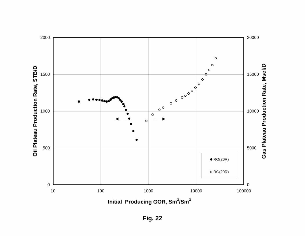
Fig. 22

0

500

1000

1500

2000

10 100 1000 10000 100000


Oil

Pla

teau

Pro

du

ctio

n R

ate,

ST

B/D

0

5000

10000

15000

20000

Gas

Pla

teau

Pro

du

ctio

n R

ate,

Msc

f/D

RO(20R)

RG(20R)

Fig. 23

0

500

1000

1500

2000

10 100 1000 10000 100000


Oil

Pla

teau

Pro

du

ctio

n R

ate,

ST

B/D

0

5000

10000

15000

20000

Gas

Pla

teau

Pro

du

ctio

n R

ate,

Msc

f/D

RO(MB) RO(20R)

RG(MB) RG(20R)

a

c

b

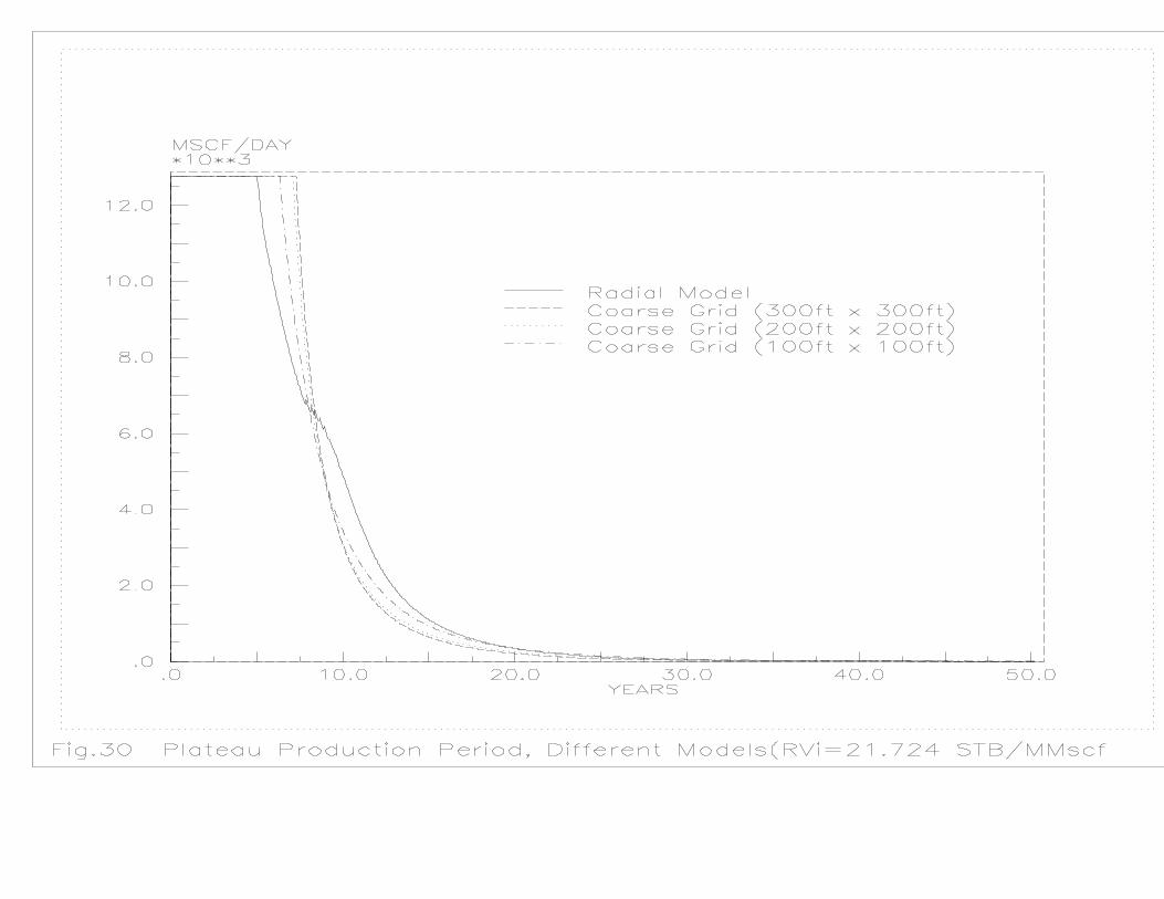
Fig. 32

0

2

4

6

8

10

10 100 1000 10000 100000


Pla

teau

Pro

du

ctio

n P

erio

d, y

rs

RO(20R) RG(2OR)

RO(100) RG(100)

RO(200) RG(200)

RO(300) RG(300)

Fig. 33

0.00

0.10

0.20

0.30

0.40

0.50

10 100 1000 10000 100000


Dec

line

Co

nst

ant,

/yr

RO(MB) RG(MB)

RO(20R) RG(20R)

reservoir performance of fluid systems with widely...

Documents