reservoir modeling of co2 injection in arbuckle saline ... · reservoir modeling of co 2 injection...
TRANSCRIPT

Reservoir Modeling of CO2 Injection in Arbuckle Saline Aquifer at Wellington Field, Sumner County, Kansas
Type of Report: Topical
Principal Author: Yevhen Holubnyak Contributors: Willard Watney, Tiraz Birdie, Jason Rush, and Mina Fazelalavi
Kansas Geological Survey and Tbirdie Consulting
Date Report was issued: October 2016 DOE Award No: DE-FE-0006821
Name of Submitting Organization: Kansas Geological Survey
University of Kansas Center for Research 2385 Irving Hill Road Lawrence, KS 66047
Kansas Geological Survey Open-File Report 2016-29 Disclaimer This report was prepared as an account of work sponsored by an agency of the United States Government. Neither the United States Government nor any agency thereof, nor any of their employees, makes any warranty, express or implied, or assumes any legal liability or responsibility for the accuracy, completeness, or usefulness of any information, apparatus, product, or process disclosed, or represents that its use would not infringe privately owned rights. Reference herein to any specific commercial product, process, or service by trade name, trademark, manufacturer, or otherwise does not necessarily constitute or imply its endorsement, recommendation, or favoring by the United States Government or any agency thereof. The views and opinions of authors expressed herein do not necessarily state or reflect those of the United States Government or any agency thereof.

Kansas Geological Survey Open-File Report 2016-29 2
1. IntroductionThis section presents details of the Arbuckle reservoir simulation model that was
constructed to project the results of the Wellington Field short-term Arbuckle CO2 pilot injection
project and delineate the EPA Area of Review (AoR). Work was performed under
DEFE0006821 to fulfill Task 18—Reside Site Characterization Models and Simulations for
Carbon Storage. As required under §146.84(c) of EPA Class VI Well rule, the AoR must be
delineated using a computational model that can accurately predict the projected lateral and
vertical migration of the CO2 plume and formation fluids in the subsurface from the
commencement of injection activities until the plume movement ceases and until pressure
differentials sufficient to cause the movement of injected fluids or formation fluids into a
underground source of drinking water USDW are no longer present. The model must:
i. Be based on detailed geologic data collected to characterize the injection zone(s), con-
fining zone(s), and any additional zones; and anticipated operating data, including
injection pressures, rates, and total volumes over the proposed life of the geologic
sequestration project;
ii. Take into account any geologic heterogeneities, other discontinuities, data quality, and
their possible impact on model predictions; and
iii. Consider potential migration through faults, fractures, and artificial penetrations.
This section presents the reservoir simulations conducted to fulfill §146.84 requirements
stated above. The simulations were conducted assuming a maximum injection of 40,000 metric
tons of CO2 over a period of nine months. Based on market conditions, KGS/Berexco now plans
to inject a total of only 26,000 tons at the rate of 150 tons/day for a total period of approximately
175 days. The simulation results, therefore, represent impacts of the maximum quantity of CO2
that was originally planned for the Wellington project. The modeling results indicate that the
induced pore pressures in the Arbuckle aquifer away from the injection well are of insufficient
magnitude to cause the Arbuckle brines to migrate up into the USDW even if there were any
artificial or natural penetration in the Arbuckle Group or the overlying confining units.
The simulation results also indicate that the free-phase CO2 plume is contained within
the total CO2 plume (i.e., in the free plus dissolved phases) and that it extends to a maximum
lateral distance of 2,150 ft from the injection well. The EPA Area of Review (AoR) is defined by

Kansas Geological Survey Open-File Report 2016-29 3
the 1% saturation isoline of the stabilized free-phase plume.
2. Conceptual Model and Arbuckle Hydrogeologic State Information 2.1 ModeledFormation
The simulation model spans the entire thickness of the Arbuckle aquifer. The CO2 is to be
injected in the lower portion of the Arbuckle in the interval 4,910–5,050 feet, which has
relatively high permeability based on the core data collected at the site. Preliminary simulations
indicated that the bulk of the CO2 will remain confined in the lower portions of the Arbuckle
because of the low permeability intervals in the baffle zones and also shown in analysis of
geologic logs at wells KGS 1-28 and KGS 1-32. Therefore, no-flow boundary conditions were
specified along the top of the Arbuckle. The specification of a no-flow boundary at the top is also
in agreement with hydrogeologic analyses presented, which indicate that the upper confining
zone—comprising the Simpson Group, the Chattanooga Shale, and the Pierson formation—has
very low permeability, which should impede any vertical movement of groundwater from the
Arbuckle Group. Evidence for sealing integrity of the confining zone and absence of
transmissive faults include the following:
1) under-pressured Mississippian group of formations relative to pressure gradient in the
Arbuckle,
2) elevated chlorides in Mississippian group of formations relative to brine recovered at the
top of the Arbuckle,
3) geochemical evidence for stratification of Arbuckle aquifer system and presence of a
competent upper confining zone.
Additionally, entry pressure analyses indicate that an increase in pore pressure of more
than 956 psi within the confining zone at the injection well site is required for the CO2-brine to
penetrate through the confining zone. As discussed in the model simulation results section
below, the maximum increase in pore pressure at the top of the Arbuckle is less than 1.5 psi
under the worst-case scenario (which corresponds to a low permeability–low porosity alternative
model case as discussed in Section 5.10). This small pressure rise at the top of the Arbuckle is
due to CO2 injection below the lower vertical-permeability baffle zones present in the middle of
the Arbuckle Group, which confines the CO2 in the injection interval in the lower portions of the
Arbuckle Group. The confining zone is also documented to be locally free of transmissive
Kansas Geological Survey Open-File Report 2016-29 4
fractures based on fracture analysis conducted at KGS 1-28 (injection well). There are no known
transmissive faults in the area. It should be noted that an Operation Plan For Safe and Efficient
Injection has been submitted to the EPA, which has a provision for immediate cessation of
injection should an anomalous pressure drop be detected owing to development or opening of
fractures.
Based on the above evidence, it is technically appropriate to restrict the simulation region
within the Arbuckle Group for purposes of numerical efficiency, without compromising
predictions of the effects of injection on the plume or pressure fronts. Because of the presence of
the Precambrian granitic basement under the Arbuckle Group, which is expected to provide
hydraulic confinement, the bottom of the model domain was also specified as a no-flow
boundary. Active, real-time pressure and temperature monitoring of the injection zone at the
injection and monitoring wells will likely be able to detect any significant movement of CO2 out
of the injection zone along fractures. Also, the 18-seismometer array provided by Incorporated
Research Institutions for Seismology (IRIS) will detect small seismicity and their hypocenters
within several hundred feet resolution to provide additional means to monitor the unlikely
movement of CO2 above or below the Arbuckle injection zone.
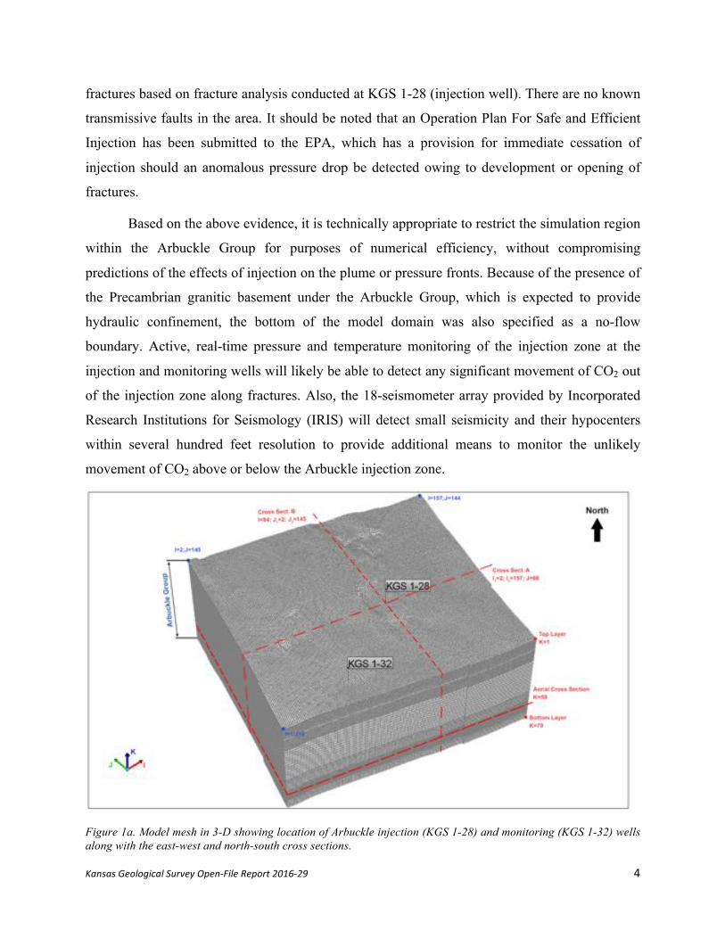
Figure 1a. Model mesh in 3-D showing location of Arbuckle injection (KGS 1-28) and monitoring (KGS 1-32) wells along with the east-west and north-south cross sections.

Kansas Geological Survey Open-File Report 2016-29 5
Figure 1b. North-south cross section of model grid along column 94 showing boundary conditions.
Kansas Geological Survey Open-File Report 2016-29 6
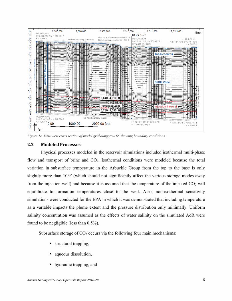
Figure 1c. East-west cross section of model grid along row 66 showing boundary conditions.
2.2 ModeledProcessesPhysical processes modeled in the reservoir simulations included isothermal multi-phase
flow and transport of brine and CO2. Isothermal conditions were modeled because the total
variation in subsurface temperature in the Arbuckle Group from the top to the base is only
slightly more than 10°F (which should not significantly affect the various storage modes away
from the injection well) and because it is assumed that the temperature of the injected CO2 will
equilibrate to formation temperatures close to the well. Also, non-isothermal sensitivity
simulations were conducted for the EPA in which it was demonstrated that including temperature
as a variable impacts the plume extent and the pressure distribution only minimally. Uniform
salinity concentration was assumed as the effects of water salinity on the simulated AoR were
found to be negligible (less than 0.5%).
Subsurface storage of CO2 occurs via the following four main mechanisms:
• structural trapping,
• aqueous dissolution,
• hydraulic trapping, and
Kansas Geological Survey Open-File Report 2016-29 7
• mineralization.
The first three mechanisms were simulated in the Wellington model. Mineralization was
not simulated as geochemical modeling indicated that due to the short-term and small- scale
nature of the pilot project, mineral precipitation is not expected to cause any problems with
clogging of pore space that may reduce permeability and negatively impact injectivity.
Therefore, any mineral storage that may occur will only result in faster stabilization of the CO2
plume and make projections presented in this model somewhat more conservative with respect to
the extent of plume migration and CO2 concentrations.
2.3 GeologicStructureThere are no transmissive faults in the Arbuckle Group that breach the overlying
confining zone in proximity to the AoR derived from the model results. The closest large
mapped fault on top of the Arbuckle and the Mississippian is approximately 12.5 mi southeast of
Wellington. The seismic data at the Wellington site also points to the absence of large faults in
the immediate vicinity of Wellington Field.
2.4 ArbuckleHydrogeologicStateInformationThe ambient pore pressure, temperature, and salinity vary nearly linearly with depth in
the Arbuckle Group. By linear extrapolation, the relationship between depth and these three
parameters can be expressed by the following equations:
Temperature (°F) = (0.011 * Depth + 73.25) Pressure (psi) = (0.487 * Depth – 324.8)
Chloride (mg/l) = (100.9 * Depth – 394.786)
Where, depth is in feet below kelly bushing (KB)
Using the above relationships, the temperature, pressure, and salinity at the top and
bottom of the Arbuckle Group at the injection well site (KGS 1-28) are presented in table 1.
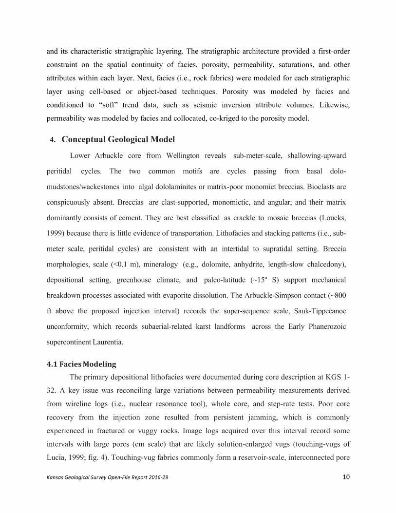
Table 1. Temperature, pressure, and salinity at the top and bottom of the Arbuckle Group at the injection well site (KGS 1-28).
Top of Arbuckle (4,168 ft) Bottom of Arbuckle (5,160 ft) Temperature (°F) 115 130
Pressure (psi) 1,705 2,188
Chloride (mg/l) 25,765 125,858

Kansas Geological Survey Open-File Report 2016-29 8
2.5 ArbuckleGroundwaterVelocityOn a regional basis, groundwater flows from east to west in the Arbuckle, as shown in the
potentiometric surface map. Groundwater velocity, however, is estimated to be very slow. The
head in Sumner County drops approximately 100 ft over 20 mi, resulting in a head gradient of
approximately 1.0e-03 ft/ft. Assuming an average large-scale Arbuckle porosity of approximately
6% and a median permeability of 10 mD based on the statistical distribution of this parameter,
the pore velocity in the Arbuckle is approximately 0.2 ft/year, which is fairly small and can be
neglected in specification of ambient boundary conditions for the purpose of this modeling study.
2.6 ModelOperationalConstraints
The bottomhole injection pressure in the Arbuckle should not exceed 90% of the
estimated fracture gradient of 0.75 psi/ft (measured from land surface). Therefore, the maximum
induced pressure at the top and bottom of the Arbuckle Group should be less than 2,813 and
3,483 psi, respectively, as specified in table 2. At the top of the perforations (4,910 ft), pressure
will not exceed 2,563 psi.
Table 2. Maximum allowable pressure at the top and bottom of the Arbuckle Group based on 90% fracture gradient of 0.675 psi/ft.
Depth (feet, bls) Maximum Pore Pressure (psi)
4,166 (Top of Arbuckle) 2,813
4,910 (Top of Perforation) 3,314
5,050 (Bottom of Perforation) 3,408
5,163 (Bottom of Arbuckle) 3,483
3. Geostatistical Reservoir Characterization of Arbuckle Group Statistical reservoir geomodeling software packages have been used in the oil and gas
industry for decades. The motivation for developing reservoir models was to provide a tool for
better reconciliation and use of available hard and soft data (fig. 2). Benefits of such numerical
models include 1) transfer of data between disciplines, 2) a tool to focus attention on critical
unknowns, and 3) a 3-D visualization tool to present spatial variations to optimize reservoir
development. Other reasons for creating high-resolution geologic models include the following:

Kansas Geological Survey Open-File Report 2016-29 9
• volumetric estimates;
• multiple realizations that allow unbiased evaluation of uncertainties before finalizing a
drilling program;
• lateral and top seal analyses;
• integration (i.e., by gridding) of 3-D seismic surveys and their derived attributes
assessments of 3-D connectivity;
• flow-simulation-based production forecasting using different well designs;
• optimizing long-term development strategies to maximize return on investment.
Figure 2. A static, geocellular reservoir model showing the categories of data that can be incorporated (source: modified from Deutsch, 2002).
Although geocellular modeling software has largely flourished in the energy industry, its
utility can be important for reservoir characterization in CO2 research and geologic storage
projects, such as the Wellington Field. The objective in the Wellington project is to integrate
various data sets of different scales into a cohesive model of key petrophysical properties,
especially porosity and permeability. The general steps for applying this technology are to model
the large-scale features followed by modeling progressively smaller, more uncertain, features.
The first step applied at the Wellington Field was to establish a conceptual depositional model
Kansas Geological Survey Open-File Report 2016-29 10
and its characteristic stratigraphic layering. The stratigraphic architecture provided a first-order
constraint on the spatial continuity of facies, porosity, permeability, saturations, and other
attributes within each layer. Next, facies (i.e., rock fabrics) were modeled for each stratigraphic
layer using cell-based or object-based techniques. Porosity was modeled by facies and
conditioned to “soft” trend data, such as seismic inversion attribute volumes. Likewise,
permeability was modeled by facies and collocated, co-kriged to the porosity model.
4. Conceptual Geological Model
Lower Arbuckle core from Wellington reveals sub-meter-scale, shallowing-upward
peritidal cycles. The two common motifs are cycles passing from basal dolo-
mudstones/wackestones into algal dololaminites or matrix-poor monomict breccias. Bioclasts are
conspicuously absent. Breccias are clast-supported, monomictic, and angular, and their matrix
dominantly consists of cement. They are best classified as crackle to mosaic breccias (Loucks,
1999) because there is little evidence of transportation. Lithofacies and stacking patterns (i.e., sub-
meter scale, peritidal cycles) are consistent with an intertidal to supratidal setting. Breccia
morphologies, scale (<0.1 m), mineralogy (e.g., dolomite, anhydrite, length-slow chalcedony),
depositional setting, greenhouse climate, and paleo-latitude (~15º S) support mechanical
breakdown processes associated with evaporite dissolution. The Arbuckle-Simpson contact (~800
ft above the proposed injection interval) records the super-sequence scale, Sauk-Tippecanoe
unconformity, which records subaerial-related karst landforms across the Early Phanerozoic
supercontinent Laurentia.
4.1FaciesModelingThe primary depositional lithofacies were documented during core description at KGS 1-
32. A key issue was reconciling large variations between permeability measurements derived
from wireline logs (i.e., nuclear resonance tool), whole core, and step-rate tests. Poor core
recovery from the injection zone resulted from persistent jamming, which is commonly
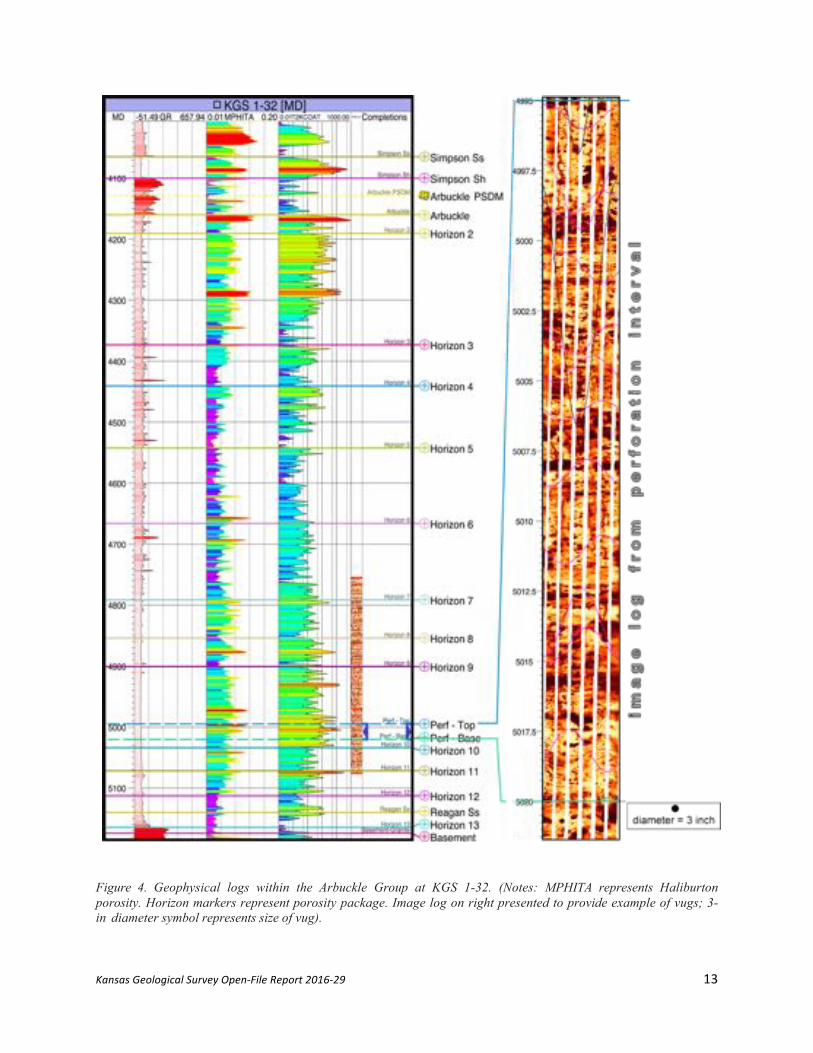
experienced in fractured or vuggy rocks. Image logs acquired over this interval record some
intervals with large pores (cm scale) that are likely solution-enlarged vugs (touching-vugs of
Lucia, 1999; fig. 4). Touching-vug fabrics commonly form a reservoir-scale, interconnected pore

Kansas Geological Survey Open-File Report 2016-29 11
system characterized by Darcy-scale permeability. It is hypothesized that a touching-vug pore
system preferentially developed within fracture-dominated crackle and mosaic breccias—formed
in response to evaporite removal—which functioned as a strataform conduit for undersaturated
meteoric fluids (fig. 5). As such, this high-permeability, interwell-scale, touching-vug pore
system is largely strataform and, therefore, predictable.
Figure 3. Example of the carbonate facies and porosity in the injection zone in the lower Arbuckle (part of the Gasconade Dolomite Formation). Upper half is light olive-gray, medium-grained dolomitic packstone with crackle breccia. Scattered subvertical fractures and limited cross stratification. Lower half of interval shown has occasional large vugs that crosscut the core consisting of a light olive-gray dolopackstone that is medium grained. Variable-sized vugs range from cm-size irregular to subhorizontal.
4.2PetrophysicalPropertiesModelingThe approach taken for modeling a particular reservoir can vary greatly based on available
information and often involves a complicated orchestration of well logs, core analysis, seismic
surveys, literature, depositional analogs, and statistics. Because well log data were available in
only two wells (KGS 1-28 and KGS 1-32) that penetrate the Arbuckle reservoir at the Wellington
site, the geologic model also relied on seismic data, step-rate test, and drill-stem test information.
Schlumberger’s Petrel™ geologic modeling software package was used to produce the current
geologic model of the Arbuckle saline aquifer for the pilot project area. This geomodel extends
1.3 mi by 1.2 mi laterally and is approximately 1,000 ft in thickness, spanning the entire

Kansas Geological Survey Open-File Report 2016-29 12
Arbuckle Group as well as a portion of the sealing units (Simpson/Chattanooga shale).
4.3 Porosity Modeling In contrast to well data, seismic data are extensive over the reservoir and are, therefore, of
great value for constraining facies and porosity trends within the geomodel. Petrel’s volume
attribute processing (i.e., genetic inversion) was used to derive a porosity attribute from the
prestack depth migration (PSDM) volume to generate the porosity model (fig. 6). The seismic
volume was created by re-sampling (using the original exact amplitude values) the PSDM 50 ft
above the Arbuckle and 500 ft below the Arbuckle (i.e., approximate basement). The cropped
PSDM volume and conditioned porosity logs were used as learning inputs during neural
network processing.
A correlation threshold of 0.85 was selected and 10,000 iterations were run to provide
the best correlation. The resulting porosity attribute was then re-sampled, or upscaled (by
averaging), into the corresponding 3-D property grid cell.
The porosity model was constructed using sequential Guassian simulation (SGS). The
porosity logs were upscaled using arithmetic averaging. The raw upscaled porosity histogram
was used during SGS. The final porosity model was then smoothed. The following
parameters were used as inputs:
I. Variogram
a. Type: spherical
b. Nugget: 0.001
c. Anisotropy range and orientation
i. Lateral range (isotropic): 5,000 ft
ii. Vertical range: 10 ft
II. Distribution: actual histogram range (0.06–0.11) from upscaled logs
III. Co-Kriging
a. Secondary 3-D variable: inverted porosity attribute grid
b. Correlation coefficient: 0.75
Kansas Geological Survey Open-File Report 2016-29 13
Figure 4. Geophysical logs within the Arbuckle Group at KGS 1-32. (Notes: MPHITA represents Haliburton porosity. Horizon markers represent porosity package. Image log on right presented to provide example of vugs; 3-in diameter symbol represents size of vug).

Kansas Geological Survey Open-File Report 2016-29 14
Figure 5. Classification of breccias and clastic deposits in cave systems exhibiting relationship between chaotic breccias, crackle breccias, and cave-sediment fill (source: Loucks, 1999).
Figure 6. Upscaled porosity distribution in the Arbuckle Group based on the Petrel geomodel.

Kansas Geological Survey Open-File Report 2016-29 15
4.4 Permeability Modeling
The upscaled permeability logs shown in fig. 4 were created using the following
controls: geometric averaging method; logs treated as points; and method set to simple. The
permeability model was constructed using SGS. Isotropic semi-variogram ranges were set to
3,000 ft horizontally and 10 ft vertically. The permeability was collocated and co-Kriged to the
porosity model using the calculated correlation coefficient (~0.70). The resulting SGS-based
horizontal and vertical permeability distributions are presented in fig. 7a–f, which shows the
relatively high permeability zone selected for completion within the injection interval. Table 3
presents the minimum, maximum, and average permeabilities within the Arbuckle Group in the
geomodel.
Table 3. Hydrogeologic property statistics in hydrogeologic characterization and simulation models.
Reservoir Characterization Geomodel Reservoir Simulation Numerical Model
Property min max avg min max avg
Porosity (%) 3.2 12.9 6.8 3.2 12.9 6.7
Horizontal Permeability (mD) 0.05 23,765 134.2 0.05 23,765 130.7
Vertical Permeability (mD) .005 1,567 387 0.005 1,567 385
5. Arbuckle Reservoir Flow and Transport Model Extensive computer simulations were conducted to estimate the potential impacts of
CO2 injection in the Arbuckle injection zone. The key objectives were to determine the
resulting rise in pore pressure and the extent of CO2 plume migration. The underlying
motivation was to determine whether the injected CO2 could affect the USDW or potentially
escape into the atmosphere through existing wells or hypothetical faults/fractures that might be
affected by the injected fluid.
As in all reservoirs, there are data gaps that prevent an absolute or unique
characterization of the geology and petrophysical properties. This results in conceptual,
parametric, and boundary condition uncertainties. To address these uncertainties,
comprehensive simulations were conducted to perform a sensitivity analysis using alternative
parameter sets. A key objective was to derive model parameter sets that would result in the
Kansas Geological Survey Open-File Report 2016-29 16
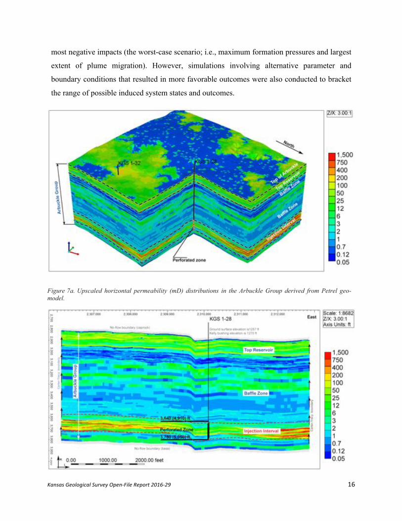
most negative impacts (the worst-case scenario; i.e., maximum formation pressures and largest
extent of plume migration). However, simulations involving alternative parameter and
boundary conditions that resulted in more favorable outcomes were also conducted to bracket
the range of possible induced system states and outcomes.
Figure 7a. Upscaled horizontal permeability (mD) distributions in the Arbuckle Group derived from Petrel geo-model.
Kansas Geological Survey Open-File Report 2016-29 17
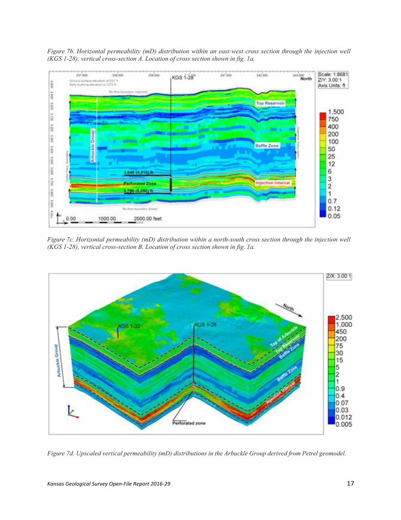
Figure 7b. Horizontal permeability (mD) distribution within an east-west cross section through the injection well (KGS 1-28), vertical cross-section A. Location of cross section shown in fig. 1a.
Figure 7c. Horizontal permeability (mD) distribution within a north-south cross section through the injection well (KGS 1-28), vertical cross-section B. Location of cross section shown in fig. 1a.
Figure 7d. Upscaled vertical permeability (mD) distributions in the Arbuckle Group derived from Petrel geomodel.
Kansas Geological Survey Open-File Report 2016-29 18
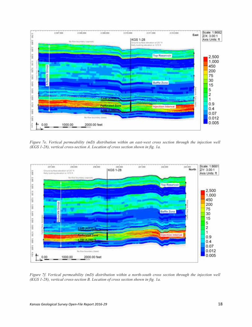
Figure 7e. Vertical permeability (mD) distribution within an east-west cross section through the injection well (KGS 1-28), vertical cross-section A. Location of cross section shown in fig. 1a.
Figure 7f. Vertical permeability (mD) distribution within a north-south cross section through the injection well (KGS 1-28), vertical cross-section B. Location of cross section shown in fig. 1a.

Kansas Geological Survey Open-File Report 2016-29 19
5.2 SimulationSoftwareDescription
The reservoir simulations were conducted using the Computer Modeling Group
(CMG) GEM simulator. GEM is a full equation of state compositional reservoir simulator
with advanced features for modeling the flow of three-phase, multi-component fluids and has
been used to conduct numerous CO2 studies (Chang et al., 2009; Bui et al., 2010). It is
considered by DOE to be an industry standard for oil/gas and CO2 geologic storage
applications. GEM is an essential engineering tool for modeling complex reservoirs with
complicated phase behavior interactions that have the potential to impact CO2 injection and
transport. The code can account for the thermodynamic interactions between three phases:
liquid, gas, and solid (for salt precipitates). Mutual solubilities and physical properties can be
dynamic variables depending on the phase composition/system state and are subject to well-
established constitutive relationships that are a function of the system state (pressures,
saturation, concentrations, temperatures, etc.). In particular, the following assumptions govern
the phase interactions:
• Gas solubility obeys Henry’s Law (Li and Nghiem, 1986)
• The fluid phase is calculated using Schmit-Wenzel or Peng-Robinson (SW-PR)
equations of state (Søreide and Whitson, 1992)
• Changes in aqueous phase density with CO2 solubility, mineral precipitations,
etc., are accounted for with the standard or Rowe and Chou correlations.
• Aqueous phase viscosity is calculated based on Kestin, Khalifa, and Correia
(1981).
5.3 ModelMeshandBoundaryConditionsThe Petrel-based geomodel mesh discussed above consists of a 706 x 654 horizontal
grid and 79 vertical layers for a total of 36,476,196 cells. The model domain spans from the
base of the Arbuckle Group to the top of the Pierson Group. To reduce reservoir simulation
time, this model was upscaled to a 157 x 145 horizontal mesh with 79 layers for a total of
1,798,435 cells to represent the same rock volume as the Petrel model for use in the CMG
simulator. The thickness of the layers varies from 5 to 20 ft based on the geomodel, with an
average of 13 feet.
Kansas Geological Survey Open-File Report 2016-29 20
Based on preliminary simulations, it was determined that due to the small scale of
injection and the presence of a competent confining zone, the plume would be contained
within the Arbuckle system for all alternative realizations of reservoir parameters. Therefore,
the reservoir model domain was restricted to the Arbuckle aquifer with no-flow boundaries
specified along the top (Simpson Group) and bottom (Precambrian basement) of the Arbuckle
group. As discussed in Section 5.2.1, the specification of no-flow boundaries along the top and
bottom of the Arbuckle Group is justified because of the low permeabilities in the overlying
and underlying confining zones as discussed in Section 4.7.3. The permeability in the Pierson
formation was estimated to be as low as 1.6 nanoDarcy (nD; 1.0-9 Darcy).
The simulation model, centered approximately on the injection well (KGS 1-28),
extends approximately 1.2 mi in the east-west and 1.3 mi in the north-south orientations.
Vertically, the model extends approximately 1,000 ft from the top of the Precambrian
basement to the bottom of the Simpson Group. As discussed above, the model domain was
discretized laterally by 157 x 145 cells in the east-west and north-south directions and
vertically in 79 layers. The lateral boundary conditions were set as an infinite-acting Carter-
Tracy aquifer (Dake, 1978; Carter and Tracy, 1960) with leakage. This is appropriate since the
Arbuckle is an open hydrologic system extending over most of Kansas. Sensitivity simulations
indicated that the increases in pore pressures and the plume extent were not meaningfully
different by using a closed boundary instead of a Carter-Tracy boundary.
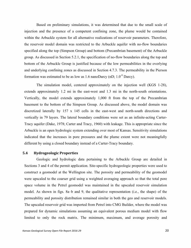
5.4 HydrogeologicPropertiesGeologic and hydrologic data pertaining to the Arbuckle Group are detailed in
Sections 3 and 4 of the permit application. Site-specific hydrogeologic properties were used to
construct a geomodel at the Wellington site. The porosity and permeability of the geomodel
were upscaled to the coarser grid using a weighted averaging approach so that the total pore
space volume in the Petrel geomodel was maintained in the upscaled reservoir simulation
model. As shown in figs. 8a–b and 9, the qualitative representation (i.e., the shape) of the
permeability and porosity distribution remained similar in both the geo and reservoir models.
The upscaled reservoir grid was imported from Petrel into CMG Builder, where the model was
prepared for dynamic simulations assuming an equivalent porous medium model with flow
limited to only the rock matrix. The minimum, maximum, and average porosity and

Kansas Geological Survey Open-File Report 2016-29 21
RT RQIfrom RQITo AveRQI1 40 10 252 10 2.5 6.253 2.5 1 1.754 1 0.5 0.755 0.5 0.4 0.456 0.4 0.3 0.357 0.3 0.2 0.258 0.2 0.1 0.159 0.1 0.01 0.055
RQI
permeabilities in the reservoir model are documented in table 3 alongside the statistics for the
geomodel.
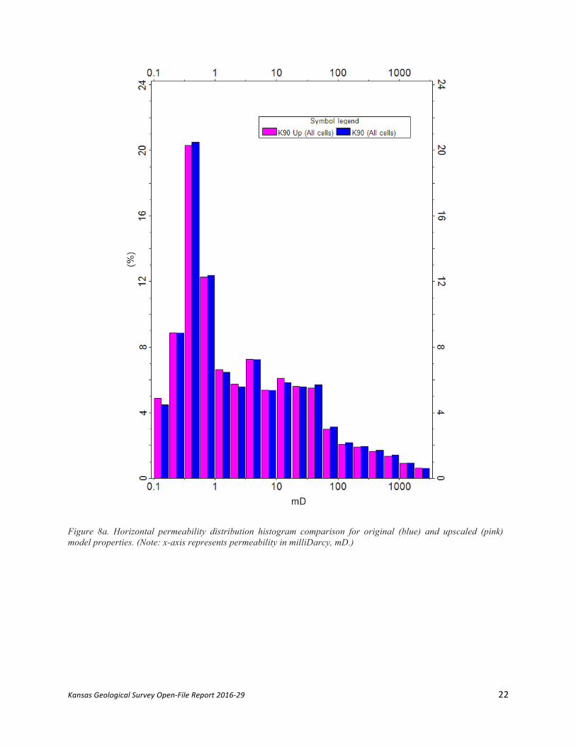
5.5 RockTypeAssignment
Nine rock types and corresponding tables with capillary pressure hysteresis were
developed based on reservoir quality index (RQI) ranges, where RQI is calculated for each grid
cell using the formula:
!"# = 0.0314 !"#$ !"#"$%&'
Using RQI ranges, rock types are assigned using CMG Builder’s Formula Manager. The
resulting maps of rock type distribution in the model are shown in fig. 10a–c. The division of the
nine rock-types (RT) was based on dividing the irreducible water saturation into nine ranges to
find their equivalent RQI as shown in table 4. Relative permeability and capillary pressure
curves were calculated for each of the nine RQI values.
Table 4.RQI and Relative Permeability Types assignments (RT)
Kansas Geological Survey Open-File Report 2016-29 22
Figure 8a. Horizontal permeability distribution histogram comparison for original (blue) and upscaled (pink) model properties. (Note: x-axis represents permeability in milliDarcy, mD.)

Kansas Geological Survey Open-File Report 2016-29 23
Figure 8b. Vertical permeability distribution histogram comparison for original (blue) and upscaled (pink) model properties. (Note: x-axis represents permeability in milliDarcy, mD.)

Kansas Geological Survey Open-File Report 2016-29 24
Figure 9. Porosity distribution histogram comparison for original and upscaled model properties. (Note: x-axis represents porosity.)
Kansas Geological Survey Open-File Report 2016-29 25
Figure 10a. Rock type distribution model.
Figure 10b. Rock type distribution model, distribution within an east-west cross section through the injection well
(KGS 1-28), vertical cross-section A.

Kansas Geological Survey Open-File Report 2016-29 26
Figure 10c. Rock type distribution within a north-south cross section through the injection well (KGS 1-28),
vertical cross-section B.
5.6 RelativePermeability
Nine sets of relative permeability curves for both drainage and imbibition were
calculated for the nine rock types. These sets of relative permeability curves were calculated
based on a recently patented formula (SMH reference No: 1002061-0002) that relates the end
points to RQI, thereby resulting in a realistic relative permeability data set. The validation of the
method is presented below under Validation of the Capillary Pressure and Relative Permeability
Methods. Literature experimental studies, including Krevor and Benson (2012, 2015), indicate
that the maximum experimental CO2 saturation (SCO2max) and maximum CO2 relative
permeability (KrCO2max) in higher permeability samples typically do not reach their actual
values and are lower than expected. The authors note that the cause of low experimental end
points are the unattainable high capillary pressure in the high permeability core samples.
Calculations based on the new patented method addresses and resolves this issue. The highest
maximum CO2 relative permeability (KrCO2 max) for drainage curves from literature (Bennion
and Bachu, 2007) is 0.54, which is lower than expected; however, the highest maximum CO2
relative permeability using the new method is 0.71, which is a more realistic value. As noted
above, measured relative permeabilities from literature do not represent the end points of
relative permeability curves and they need to be adjusted. Using this new method, SCO2max and

Kansas Geological Survey Open-File Report 2016-29 27
KrCO2max are scaled up to reasonable values.
Highest and lowest Corey CO2 exponent values from Bennion and Bachu (2010) were
selected and they were assigned to the nine RQI values in a descending order from high to low.
The full range of RQI assignments and relative permeability tables can be found in Appendix B.
An example of capillary pressure and relative permeability for both drainage and imbibition is
presented in table 5. Corey Water exponents for different permeabilities from literature did not
show much variability. Therefore, average values were used for both drainage and imbibition
curves. Figure 11a presents relative permeability curves for an RQI value of 0.35 for illustrative
purposes. Figure 11b presents the same set of curves for the full range of RQI values. Residual
CO2 saturation (SCO2r) for calculating imbibition curves was needed. SCO2r was calculated
based on a correlation between residual CO2 saturation (SCO2r) and initial CO2 saturation
(SCO2i) (Burnside and Naylor, 2014).
Figure 11a. Calculated relative permeability for drainage (left) and imbibition (right) for RQI=0.35.

Kansas Geological Survey Open-File Report 2016-29 28
Figure 11b. Calculated relative permeability for drainage (top) and imbibition (bottom) for full set of RQI.
Kansas Geological Survey Open-File Report 2016-29 29
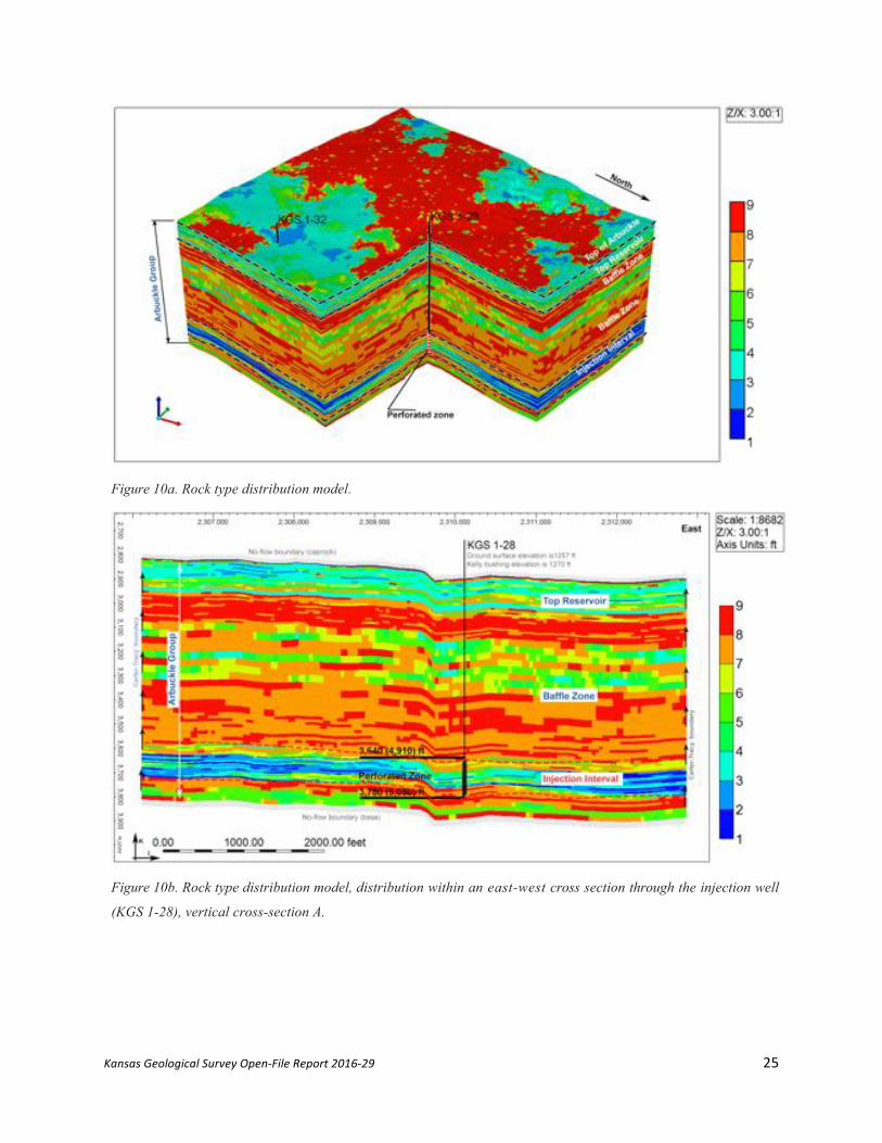
Table 5. Example of capillary pressure and relative permeability drainage and imbibition tables for rock type 6 (RQI=0.35).
Drainage Curves
Imbibition Curves RQI range from 0.3-0.4-AveRQI=0.35
RQI range from 0.3-0.4-AveRQI=0.35
Pc Sw SCO2 Krw krCO2
Pc Sw SCO2 Krw krCO2 1 1.000 0.000 1.000 0.000
0 0.666 0.334 0.331 0.000
2 0.877 0.123 0.735 0.001
0.00 0.665 0.335 0.328 0.000 3 0.641 0.359 0.338 0.029
0.01 0.663 0.337 0.325 0.000
4 0.518 0.482 0.190 0.086
0.02 0.660 0.340 0.319 0.000 5 0.443 0.557 0.119 0.148
0.03 0.657 0.343 0.313 0.000
6 0.392 0.608 0.080 0.205
0.04 0.654 0.346 0.308 0.000 7 0.354 0.646 0.056 0.257
0.05 0.652 0.348 0.302 0.000
8 0.326 0.674 0.041 0.302
0.06 0.649 0.351 0.297 0.000 9 0.304 0.696 0.030 0.341
0.07 0.646 0.354 0.292 0.000
10 0.286 0.714 0.023 0.375
0.08 0.643 0.357 0.287 0.000 12 0.258 0.742 0.013 0.432
0.09 0.640 0.360 0.282 0.001
14 0.238 0.762 0.008 0.478
0.1 0.638 0.362 0.277 0.001 18 0.211 0.789 0.003 0.545
0.2 0.612 0.388 0.234 0.003
20 0.201 0.799 0.002 0.571
0.3 0.589 0.411 0.200 0.008 25 0.183 0.817 0.000 0.620
0.4 0.569 0.431 0.171 0.013
30 0.171 0.829 0.000 0.655
0.5 0.550 0.450 0.148 0.020 40 0.156 0.844 0.000 0.655
0.6 0.532 0.468 0.128 0.029
50 0.146 0.854 0.000 0.655
0.7 0.516 0.484 0.112 0.038 60 0.140 0.860 0.000 0.655
0.8 0.501 0.499 0.098 0.047
70 0.135 0.865 0.000 0.655
0.9 0.487 0.513 0.086 0.057 80 0.131 0.869 0.000 0.655
1 0.474 0.526 0.076 0.067
90 0.129 0.871 0.000 0.655
2 0.383 0.617 0.026 0.172 100 0.126 0.874 0.000 0.655
3 0.329 0.671 0.011 0.261
150 0.119 0.881 0.000 0.655
4 0.293 0.707 0.005 0.333 200 0.116 0.884 0.000 0.655
5 0.267 0.733 0.002 0.390
300 0.112 0.888 0.000 0.655
6 0.248 0.752 0.001 0.437
7 0.233 0.767 0.001 0.476
8 0.221 0.779 0.000 0.508
9 0.211 0.789 0.000 0.536
10 0.203 0.797 0.000 0.559
12 0.189 0.811 0.000 0.598
14 0.180 0.820 0.000 0.629
20 0.160 0.840 0.000 0.655
30 0.144 0.856 0.000 0.655
40 0.135 0.865 0.000 0.655
50 0.129 0.871 0.000 0.655
60 0.126 0.874 0.000 0.655
70 0.123 0.877 0.000 0.655
80 0.121 0.879 0.000 0.655
90 0.119 0.881 0.000 0.655
100 0.117 0.883 0.000 0.655
150 0.113 0.887 0.000 0.655
200 0.111 0.889 0.000 0.655
300 0.109 0.891 0.000 0.655
5.7 CapillaryPressureCurves
Nine capillary pressure curves were calculated for drainage and imbibition for nine RQI
values based on a recently patented formula (SMH reference No: 1002061-0002). The formula
constitutes a function for the shape of Pc curves and functions for the end points that are entry
pressure (Pentry) and irreducible water saturation (Swir). The end points are correlated to RQI.
Pentry was calculated from entry radius (R15) and Winland (R35). There is a relationship

Kansas Geological Survey Open-File Report 2016-29 30
between R35 and R15 and a relationship between Pentry and R15; therefore, Pentry can be
calculated from R15 derived from R35. Swir was calculated from the NMR log at a Pc equal to
20 bars (290 psi). To calculate imbibition curves, a residual CO2 saturation (CO2r) value was
needed. CO2r was calculated from a relationship between initial CO2 saturation and CO2r as
discussed above. The capillary pressure curves for drainage and imbibition for RQI of 0.35 are
presented in fig. 12. The capillary pressure data for the full set of RQI values are presented in
Appendix B.
Figure 12. Capillary pressure curves for drainage (left) and imbibition (right) for an RQI value of 0.35.
5.8 ValidationoftheCapillaryPressureandRelativePermeabilityMethodsThe capillary pressure and relative permeability curves were estimated in the
laboratory for the Mississippian Reservoir as part of the Wellington Mississippian Enhanced
Oil Recovery (EOR) project located approximately a mile southwest of the Wellington CO2
storage site. The laboratory-derived curves were used to validate the relative permeability and
capillary pressure approach for the Arbuckle discussed above and this was deemed reasonable
since the same approach that was used in the Mississippian was also used for the Arbuckle.
Two core plug samples with similar RQI values were sent to Core Laboratories for
capillary pressure and relative permeability measurements. The relative permeability and
capillary pressure curves were calculated twice for the Mississippian reservoir—before and
after the core results were obtained from the laboratory. The initial estimation of Pc curves was
based on the end points that were calculated from the NMR log. As shown in fig. 13a, there is a

Kansas Geological Survey Open-File Report 2016-29 31
slight difference between the calculated Pc and measured Pc before calibration. However, there
is an excellent match between the calculated Pc and the measured Pc after calibration using the
core measured end points. Similarly, as shown in fig. 13b, there is a slight difference between
the initial calculated relative permeability and measured relative permeability, but the match is
excellent after calibration.
Figure 13a. Capillary pressure curves for an RQI value of 0.2 before calibration (left) and after calibration (right).
Figure 13b. Relative permeability curves for an RQI value of 0.16 before calibration (left) and after calibration (right).

Kansas Geological Survey Open-File Report 2016-29 32
5.9 InitialConditionsandInjectionRates
Table 6 lists the initial conditions specified in the reservoir model. The simulations were
conducted assuming isothermal conditions, but a thermal gradient of 0.008 °C/ft was considered
for specifying petrophysical properties that vary with layer depth and temperature such as CO2
relative permeability, CO2 dissolution in formation water, etc. The original static pressure in the
injection zone (at a reference depth of 4,960 ft) was set to 2,093 psi and the Arbuckle pressure
gradient of 0.48 psi/ft was assumed for specifying petrophysical properties. A 140 ft thick
perforation zone in well KGS 1-28 was specified between 4,910 and 5,050 ft. A constant brine
density of 68.64 lbs/ft3 (specific gravity of 1.1) was assumed. A total of 40,000 metric tons
(MT) of CO2 was injected in the Arbuckle formation over a period of nine months at an average
injection rate of 150 tons/day.
Table 6. Model input specification and CO2 injection rates.
Temperature 60 °C (140 oF)
Temperature Gradient 0.008 °C/ft
Pressure 2,093 psi (14.43 MPa) @ 4,960 ft RKB
Perforation Zone 4,910-5,050 ft
Perforation Length 140 ft (model layers 54 to 73)
Injection Period 9 months
Injection Rate 150 tons/day
Total CO2 injected 40,000 MT
5.10 PermeabilityandPorosityAlternativeModels
The base-case reservoir model has been carefully constructed using a sophisticated
geomodel as discussed in Section 5.3, which honors site-specific hydrogeologic information
obtained from laboratory tests and log-based analyses. However, to account and test for
sensitivity of hydrogeologic uncertainties, a set of alternate parametric models were developed
by varying the porosity and horizontal hydraulic permeability. Specifically, the porosity and
permeability were increased and decreased by 25% following general industry practice
(FutureGen Industrial Alliance, 2013). This resulted in nine alternative models, listed in table 7.
Simulation results based on all nine models were evaluated to derive the worst-case impacts on

Kansas Geological Survey Open-File Report 2016-29 33
pressure and migration of the plume front for purposes of establishing the AoR and ensuring
that operational constraints are not exceeded.
Table 7. Nine alternative permeability-porosity combination models (showing multiplier of base-case permeability and porosity distribution assigned to all model cells).
Alternative Models Base Porosity x 0.75 Base Porosity Base Porosity x 1.25
Base Permeability x 0.75 K-0.75/Phi-0.75 K-0.75/Phi-1.0 K-0.75/Phi-1.25
Base Permeability K-1.0/Phi-0.75 K-1.0/Phi-1.0 K-1.0/Phi-1.25
Base Permeability x 1.25 K-1.25/Phi-0.75 K-1.25/Phi-1.0 K-1.25/Phi-1.25
6. Reservoir Simulation Results For the simulations, 40,000 MT of CO2 were injected into the KGS 1-28 well at a
constant rate of approximately 150 tons per day for a period of nine months. Although Berexco
is seeking a permit for injecting 40,000 tons, it is likely that only 26,000 tons will be injected due
to budgetary constraints. At the request of the EPA, an alternate set of simulations were
conducted with a total injection volume of only 26,000 tons. All simulation results presented
below for 40,000 tons are repeated for an injection volume of 26,000 tons in Appendix A. Note
that only the simulation result figures are provided in Appendix A; the context for each figure is
the same as provided in the following description for an injection volume of 40,000 tons. For
example, fig. A.6a (in Appendix A), which shows the extent of the free-phase CO2 plume at six
months from commencement of injection for an injection volume of 26,000 tons is equivalent to
fig. 14a below, which shows the plume extent at six months from the start of injection for an
injection volume of 40,000 tons.
A total of nine models representing three sets of alternate permeability-porosity
combinations as specified in table 7 were simulated with the objective of bracketing the range
of expected pressures and extent of CO2 plume migration.
The extent of lateral plume migration depends on the particular combination of
permeability-porosity in each of the nine alternative models. These two parameters are
independently specified in CMG as they are assumed to be decoupled. A high-permeability
value results in farther travel of the plume due to gravity override, bouyancy, and updip
migration. Similarly, a low effective porosity for the same value of permeability results in
farther travel for the plume as compared to high porosity as the less-connected pore volume

Kansas Geological Survey Open-File Report 2016-29 34
results in faster pore velocity. The high-permeability/low-porosity combination (k-1.25/phi-
0.75) resulted in the largest horizontal plume dimension. In contrast, the highest induced
pressures were obtained for the alternative model with the lowest permeability and the lowest
porosity (k-0.75/phi-0.75).
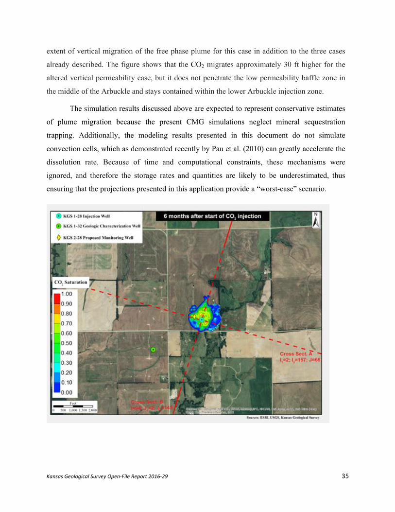
6.1 CO2PlumeMigrationFigure 14a–f shows the maximum lateral migration of the CO2 plume in the injection
interval (elevation 5,010 ft) for the largest areal migration case (k-1.25/phi-0.75). The plume
grows rapidly during the injection phase (fig. 14a–c) and is largely stabilized by the end of the
second year (fig. 14d). The plume at the end of 100 years (fig. 14f) has spread only minimally
since cessation of injection and has a maximum lateral spread of approximately 2,150 ft from
the injection well. It does not intercept any well other than the proposed Arbuckle monitoring
well KGS 2-28, will be constructed in compliance with Class VI injection well guidelines.
The evolution of the maximum lateral extent of the free phase plume is shown in fig. 15
for the maximum plume spread case (k-1.25/phi-0.75) The plume grows rapidly during the
injection period and up to the second year from commencement of injection. Thereafter, the
plume has stabilized to a maximum lateral extent of approximately 2,150 ft. The plume only
intercepts the proposed Arbuckle monitoring well KGS 2-28, which will be built to be in
compliance with Class VI design and construction requirements. There are no additional natural
or artificial penetrations that will allow CO2 to escape upward from the Arbuckle injection
zone.
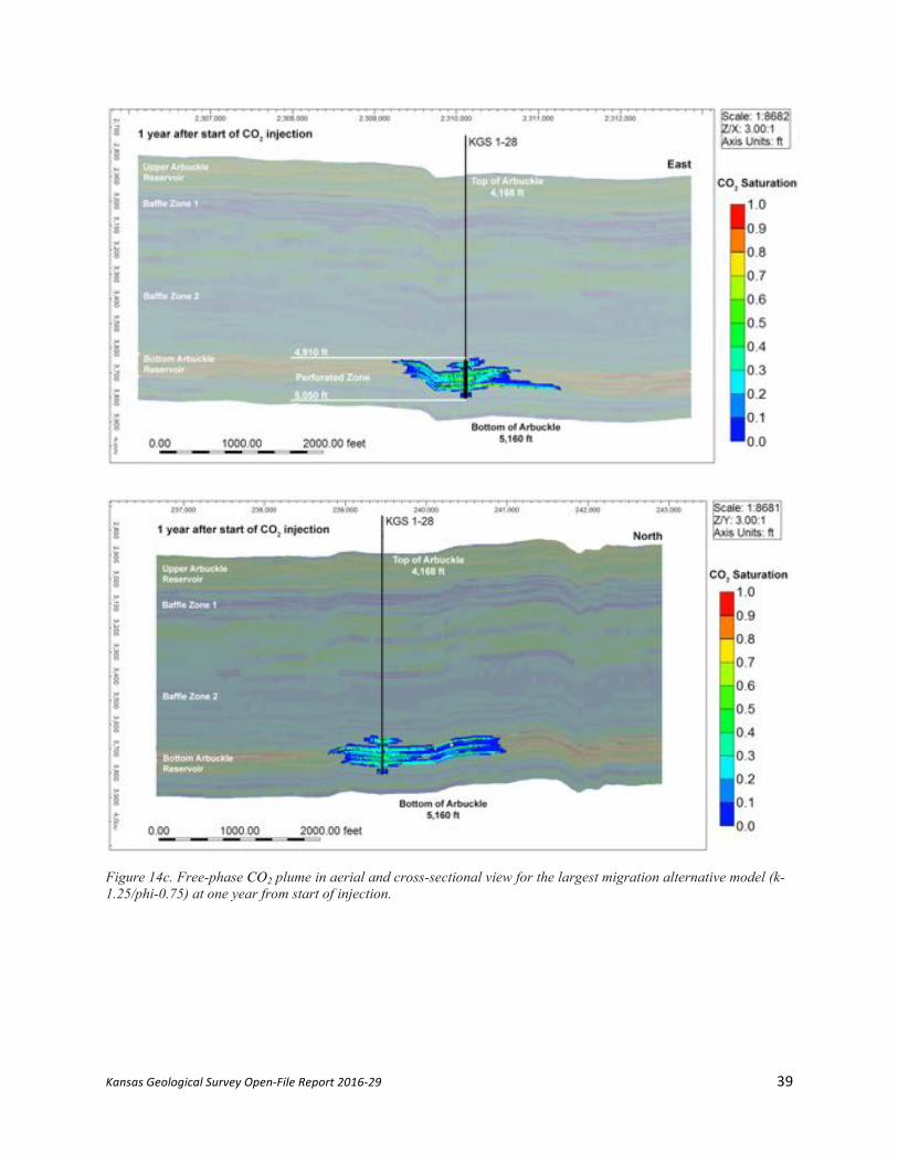
Figure 16 shows the extent of vertical plume migration for the fast vertical migration
case (k-1.25/phi-0.75), the base case (k-1.00/phi-1.00), and the high pressure case (k-0.75/phi-
0.75). The free-phase plume remains confined in the injection interval (lower Arbuckle)
because of the presence of the low-permeability baffle zones above the injection interval. This
same information is shown in fig. 14 a—f, which shows the maximum extent of vertical
migration. For all three cases, the plume remains confined in the injection interval in the lower
Arbuckle.
To account for uncertainties of CO2 movement in the vertical direction, an alternate
vertical permeability model was also developed in which the vertical permeability parameter
was increased by 50% along with a porosity of 75% (k-1.50/phi-0.75). Figure 16 presents the
Kansas Geological Survey Open-File Report 2016-29 35
extent of vertical migration of the free phase plume for this case in addition to the three cases
already described. The figure shows that the CO2 migrates approximately 30 ft higher for the
altered vertical permeability case, but it does not penetrate the low permeability baffle zone in
the middle of the Arbuckle and stays contained within the lower Arbuckle injection zone.
The simulation results discussed above are expected to represent conservative estimates
of plume migration because the present CMG simulations neglect mineral sequestration
trapping. Additionally, the modeling results presented in this document do not simulate
convection cells, which as demonstrated recently by Pau et al. (2010) can greatly accelerate the
dissolution rate. Because of time and computational constraints, these mechanisms were
ignored, and therefore the storage rates and quantities are likely to be underestimated, thus
ensuring that the projections presented in this application provide a “worst-case” scenario.

Kansas Geological Survey Open-File Report 2016-29 36
Figure 14a. Free-phase CO2 plume in aerial and cross-sectional view for the largest migration alternative model (k-1.25/phi-0.75) at six months from start of injection.
Kansas Geological Survey Open-File Report 2016-29 37

Kansas Geological Survey Open-File Report 2016-29 38
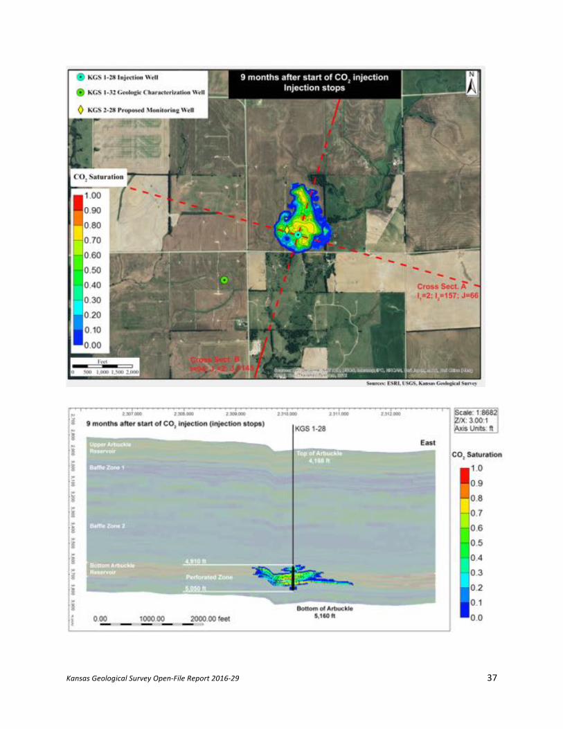
Figure 14b. Free-phase CO2 plume in aerial and cross-sectional view for the largest migration alternative model (k-1.25/phi-0.75) at nine months from start of injection.
Kansas Geological Survey Open-File Report 2016-29 39
Figure 14c. Free-phase CO2 plume in aerial and cross-sectional view for the largest migration alternative model (k-1.25/phi-0.75) at one year from start of injection.
Kansas Geological Survey Open-File Report 2016-29 40

Kansas Geological Survey Open-File Report 2016-29 41
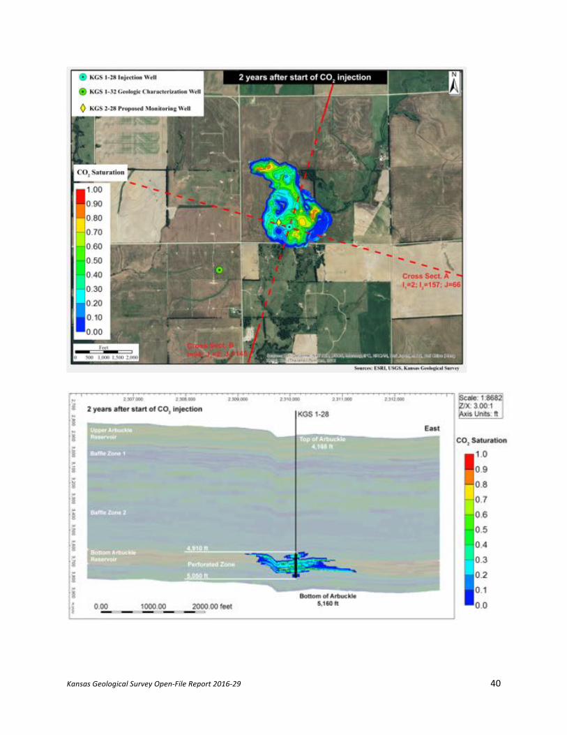
Figure 14d. Free-phase CO2 plume in aerial and cross-sectional view for the largest migration alternative model (k-1.25/phi-0.75) at two years from start of injection.

Kansas Geological Survey Open-File Report 2016-29 42
Figure 14e. Free-phase CO2 plume in aerial and cross-sectional view for the largest migration alternative model (k-1.25/phi-0.75) at 10 years from start of injection.

Kansas Geological Survey Open-File Report 2016-29 43

Kansas Geological Survey Open-File Report 2016-29 44
Figure 14f. Free-phase CO2 plume in aerial and cross-sectional view for the largest migration alternative model (k-1.25/phi-0.75) at 100 years from start of injection.
Figure 15. Maximum lateral extent of CO2 plume migration (as defined by the 0.5% CO2 saturation isoline) for the largest plume migration case k-1.25/phi-0.75.

Kansas Geological Survey Open-File Report 2016-29 45
Figure 16. Maximum vertical extent of free-phase CO2 migration for the two alternative cases that result in the maximum plume spread (k-1.25/phi-0.75) and the maximum induced pressure (k-0.75/phi-0.75) along with base case (k-1.0/phi-1.0) and vertical permeability sensitivity case (k-1.25/phi-0.75).
6.2 SimulatedTotalandDissolvedCO2SpatialDistributionFigure 17a–l shows the maximum lateral and vertical migration of the CO2 plume in total
concentration and in dissolved phase at the injection interval (elevation 5,010 ft) for the largest
areal migration case (k-1.25/phi-0.75). The areal extent of total and dissolved CO2 plumes is
larger than the extent of the CO2 plume in free phase; however, these delineations are not used
for the AoR definition, since the CO2 in dissolved and other than supercritical and gaseous
phases is considered to be immobile. The total and dissolved CO2 plumes do not intercept any
well other than the proposed Arbuckle monitoring well KGS 2-28 will be constructed in
compliance with Class VI injection well guidelines. The extent of vertical CO2 plume migration
in total and dissolved states is similar to the vertical migration of the free phase CO2. The CO2
remains confined in the injection interval (lower Arbuckle) because of the presence of the low-
permeability baffle zones above the injection interval.
4050
4150
4250
4350
4450
4550
4650
4750
4850
4950
5050
max.V
er)calM
igra)o
n,2
Time,years
MaximumVer5calMigra5onK-1.25/Phi-0.75,B MaximumVer5calMigra5onK-1/Phi-1,B
MaximumVer5calMigra5onK-0.75/Phi-0.75,B MaximumVer5calMigra5onKv1.5
Kansas Geological Survey Open-File Report 2016-29 46

Kansas Geological Survey Open-File Report 2016-29 47
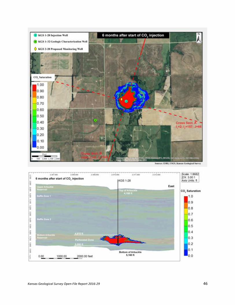
Figure 17a. Total CO2 spatial distribution in aerial and cross-sectional view for the largest migration alternative model (k-1.25/phi-0.75) at six months from start of injection.
Kansas Geological Survey Open-File Report 2016-29 48
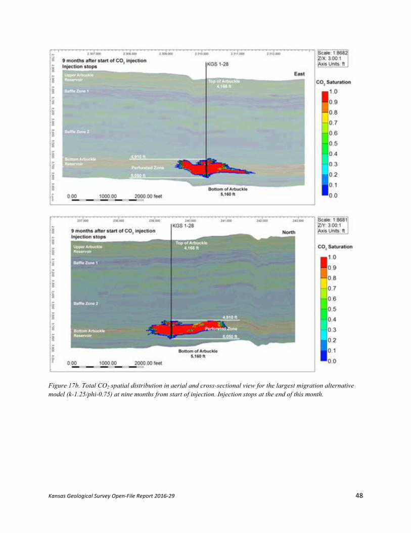
Figure 17b. Total CO2 spatial distribution in aerial and cross-sectional view for the largest migration alternative model (k-1.25/phi-0.75) at nine months from start of injection. Injection stops at the end of this month.

Kansas Geological Survey Open-File Report 2016-29 49

Kansas Geological Survey Open-File Report 2016-29 50
Figure 17c. Total CO2 spatial distribution in aerial and cross-sectional view for the largest migration alternative model (k-1.25/phi-0.75) at one year from start of injection.

Kansas Geological Survey Open-File Report 2016-29 51
Figure 17d. Total CO2 spatial distribution in aerial and cross-sectional view for the largest migration alternative model (k-1.25/phi-0.75) at two years from start of injection.

Kansas Geological Survey Open-File Report 2016-29 52

Kansas Geological Survey Open-File Report 2016-29 53
Figure 17e. Total CO2 spatial distribution in aerial and cross-sectional view for the largest migration alternative model (k-1.25/phi-0.75) at 10 years from start of injection.

Kansas Geological Survey Open-File Report 2016-29 54
Figure 17f. Total CO2 spatial distribution in aerial and cross-sectional view for the largest migration alternative model (k-1.25/phi-0.75) at 100 years from start of injection.

Kansas Geological Survey Open-File Report 2016-29 55

Kansas Geological Survey Open-File Report 2016-29 56
Figure 17g. Dissolved CO2 spatial distribution in aerial and cross-sectional view for the largest migration alternative model (k-1.25/phi-0.75) at six months from start of injection.

Kansas Geological Survey Open-File Report 2016-29 57
Figure 17h. Dissolved CO2 spatial distribution in aerial and cross-sectional view for the largest migration alternative model (k-1.25/phi-0.75) at nine months from start of injection. Injection stops at the end of this month.

Kansas Geological Survey Open-File Report 2016-29 58
Kansas Geological Survey Open-File Report 2016-29 59
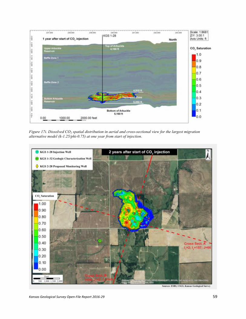
Figure 17i. Dissolved CO2 spatial distribution in aerial and cross-sectional view for the largest migration alternative model (k-1.25/phi-0.75) at one year from start of injection.

Kansas Geological Survey Open-File Report 2016-29 60
Figure 17j. Dissolved CO2 spatial distribution in aerial and cross-sectional view for the largest migration alternative model (k-1.25/phi-0.75) at two years from start of injection.

Kansas Geological Survey Open-File Report 2016-29 61

Kansas Geological Survey Open-File Report 2016-29 62
Figure 17k. Dissolved CO2 spatial distribution in aerial and cross-sectional view for the largest migration alternative model (k-1.25/phi-0.75) at 10 years from start of injection.

Kansas Geological Survey Open-File Report 2016-29 63
Figure 17l. Dissolved CO2 spatial distribution in aerial and cross-sectional view for the largest migration alternative model (k-1.25/phi-0.75) at 100 years from start of injection.
6.3 SimulatedPressureDistributionFigure 18 presents the bottomhole pressure (at a reference depth of 5,050 ft) for the
highest pressures alternative model (k-0.75/phi-0.75). The pressure increases to 2,485 psi upon
commencement of injection and then gradually drops during the injection period as the capillary
effects are overcome. The pressure decreases to pre-injection levels upon cessation of injection.
The rise in pressure to 2,485 psi upon commencement of injection represents an increase of 392 psi
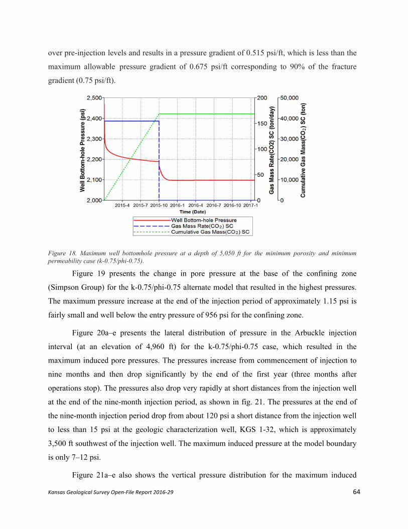
Kansas Geological Survey Open-File Report 2016-29 64
over pre-injection levels and results in a pressure gradient of 0.515 psi/ft, which is less than the
maximum allowable pressure gradient of 0.675 psi/ft corresponding to 90% of the fracture
gradient (0.75 psi/ft).
Figure 18. Maximum well bottomhole pressure at a depth of 5,050 ft for the minimum porosity and minimum permeability case (k-0.75/phi-0.75).
Figure 19 presents the change in pore pressure at the base of the confining zone
(Simpson Group) for the k-0.75/phi-0.75 alternate model that resulted in the highest pressures.
The maximum pressure increase at the end of the injection period of approximately 1.15 psi is
fairly small and well below the entry pressure of 956 psi for the confining zone.
Figure 20a–e presents the lateral distribution of pressure in the Arbuckle injection
interval (at an elevation of 4,960 ft) for the k-0.75/phi-0.75 case, which resulted in the
maximum induced pore pressures. The pressures increase from commencement of injection to
nine months and then drop significantly by the end of the first year (three months after
operations stop). The pressures also drop very rapidly at short distances from the injection well
at the end of the nine-month injection period, as shown in fig. 21. The pressures at the end of
the nine-month injection period drop from about 120 psi a short distance from the injection well
to less than 15 psi at the geologic characterization well, KGS 1-32, which is approximately
3,500 ft southwest of the injection well. The maximum induced pressure at the model boundary
is only 7–12 psi.
Figure 21a–e also shows the vertical pressure distribution for the maximum induced

Kansas Geological Survey Open-File Report 2016-29 65
pressure case (k-0.75/phi-0.75). The confining effect of the mid-Arbuckle baffle zones is
evident in the plots as the large pressure increases are mostly restricted to the injection interval.
The pressures decline rapidly at a short distance from the injection well. The pressures
throughout the model subside to nearly pre-injection levels soon after injection stops, as shown
in the one-year pressure plot in fig. 20e.
Figure 19. Change in pore pressure at the base of the confining zone (i.e., base of Simpson Group) at the injection well site for the maximum induced pressure (k-0.75/phi-0.75).

Kansas Geological Survey Open-File Report 2016-29 66

Kansas Geological Survey Open-File Report 2016-29 67
Figure 20a. Simulated increase in pressure in aerial and cross-sectional view at one month from start of injection for the low permeability–low porosity (k-0.75/phi-0.75) alternative case, which resulted in the largest simulated pressures.

Kansas Geological Survey Open-File Report 2016-29 68
Figure 20b. Simulated increase in pressure in aerial and cross-sectional view at three months from start of injection for the low permeability–low porosity (k-0.75/phi-0.75) alternative case, which resulted in the largest simulated pressures.

Kansas Geological Survey Open-File Report 2016-29 69

Kansas Geological Survey Open-File Report 2016-29 70
Figure 20c. Simulated increase in pressure in aerial and cross-sectional view at six months from start of injection for the low permeability–low porosity (k-0.75/phi-0.75) alternative case, which resulted in the largest simulated pressures.

Kansas Geological Survey Open-File Report 2016-29 71
Figure 20d. Simulated increase in pressure in aerial and cross-sectional view at nine months from start of injection for the low permeability–low porosity (k-0.75/phi-0.75) alternative case, which resulted in the largest simulated pressures.

Kansas Geological Survey Open-File Report 2016-29 72

Kansas Geological Survey Open-File Report 2016-29 73
Figure 20e.Simulated increase in pressure in aerial and cross-sectional view at one year from start of injection for the low permeability–low porosity (k-0.75/phi-0.75) alternative case, which resulted in the largest simulated pressures.
Figure 21. Pore pressure as a function of lateral distance from the injection well (KGS 1-28) at seven time intervals for the highest induced pressure case (k-0.75/phi-0.75).

Kansas Geological Survey Open-File Report 2016-29 74
Appendix A
Repeat of CMG simulations with total injected volume of 26,000 metric tons (MT) instead of 40,000 MT
For the base case simulation results presented in Section 6, 40,000 metric tons (MT) of
CO2 were injected into the KGS 1-28 well at a constant rate of approximately 150 tons per day
for a period of nine months. Although Berexco is seeking a permit for injecting 40,000 tons, it is
likely that only 26,000 tons will be injected due to budgetary constraints. At the request of the
EPA, alternate simulations were conducted with a total injection volume of only 26,000 tons. All
simulations described in Section 6 for 40,000 tons were repeated for an injection volume of
26,000 tons, and the results are presented in this appendix. Only the simulation result figures are
provided in this appendix; the context for each figure is the same as provided in the description
for an injection volume of 40,000 tons. For example, fig. A.6a (in this appendix), which shows
the extent of the plume at six months from commencement of injection for an injection volume
of 26,000 tons, is equivalent (for comparison purposes) to fig. 14a in Section 6, which shows the
plume extent at the end of six months for an injection volume of 40,000 tons.
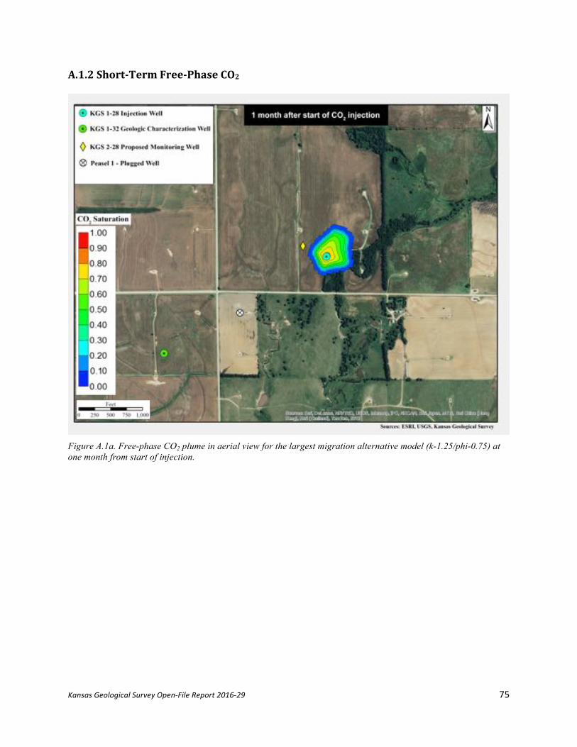
A1.CO2PlumeMigrationA1.1Short-TermCO2ArrivalForecastat(Planned)ObservationWellKGS2-28
It is projected that the dissolved CO2 will be detected and monitored with a U-Tube
sampling device at the projected observation well KGS 2-28 sometime between the first and
second month from the start of CO2 injection as indicated in fig. A.2a–b. The free phase CO2 will
arrive at the projected observation well between the fourth and fifth month after the start of the
CO2 injection (fig. A.1d–e).
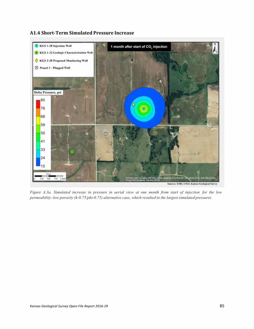
It is anticipated to detect a pore-pressure response in the projected observation well KGS
2-28 in the first seconds from the start of CO2 injection (fig. A.3a & A4). It is projected that the
maximum observed delta pore pressure at the observation well will be about 40 psi. The pressure
is projected to fall to the ambient levels within two or three months after CO2 injection has
commenced.
Kansas Geological Survey Open-File Report 2016-29 75
A.1.2Short-TermFree-PhaseCO2
Figure A.1a. Free-phase CO2 plume in aerial view for the largest migration alternative model (k-1.25/phi-0.75) at one month from start of injection.

Kansas Geological Survey Open-File Report 2016-29 76
Figure A.1b. Free-phase CO2 plume in aerial view for the largest migration alternative model (k-1.25/phi-0.75) at two months from start of injection.

Kansas Geological Survey Open-File Report 2016-29 77
Figure A.1c. Free-phase CO2 plume in aerial view for the largest migration alternative model (k-1.25/phi-0.75) at three months from start of injection.

Kansas Geological Survey Open-File Report 2016-29 78
Figure A.1d. Free-phase CO2 plume in aerial view for the largest migration alternative model (k-1.25/phi-0.75) at four months from start of injection.

Kansas Geological Survey Open-File Report 2016-29 79
Figure A.1e. Free-phase CO2 plume in aerial view for the largest migration alternative model (k-1.25/phi-0.75) at five months from start of injection.

Kansas Geological Survey Open-File Report 2016-29 80
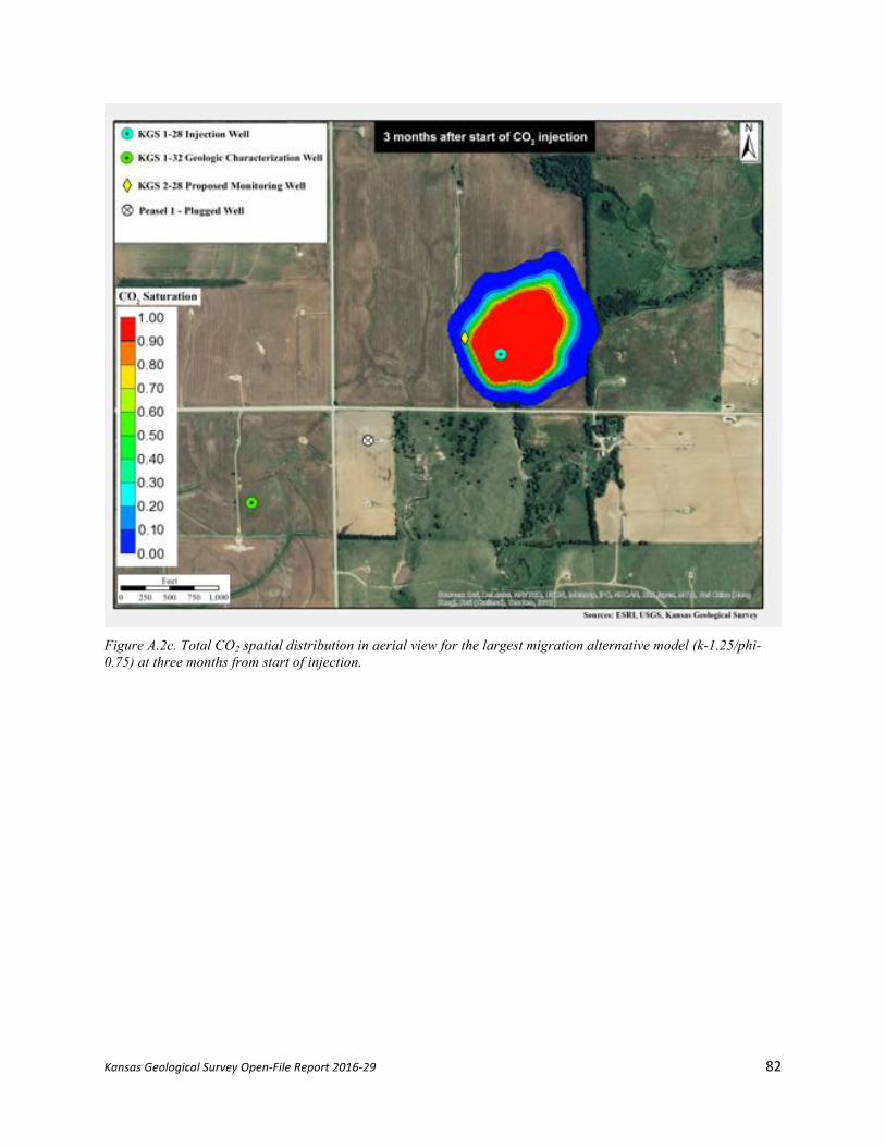
A1.3Short-TermTotalCO2SpatialDistribution
Figure A.2a. Total CO2 spatial distribution in aerial view for the largest migration alternative model (k-1.25/phi-0.75) at one month from start of injection.

Kansas Geological Survey Open-File Report 2016-29 81
Figure A.2b. Total CO2 spatial distribution in aerial view for the largest migration alternative model (k-1.25/phi-0.75) at two months from start of injection.
Kansas Geological Survey Open-File Report 2016-29 82
Figure A.2c. Total CO2 spatial distribution in aerial view for the largest migration alternative model (k-1.25/phi-0.75) at three months from start of injection.

Kansas Geological Survey Open-File Report 2016-29 83
Figure A.2d. Total CO2 spatial distribution in aerial view for the largest migration alternative model (k-1.25/phi-0.75) at four months from start of injection.

Kansas Geological Survey Open-File Report 2016-29 84
Figure A.2e. Total CO2 spatial distribution in aerial view for the largest migration alternative model (k-1.25/phi-0.75) at five months from start of injection.
Kansas Geological Survey Open-File Report 2016-29 85
A1.4Short-TermSimulatedPressureIncrease
Figure A.3a. Simulated increase in pressure in aerial view at one month from start of injection for the low permeability–low porosity (k-0.75/phi-0.75) alternative case, which resulted in the largest simulated pressures.

Kansas Geological Survey Open-File Report 2016-29 86
Figure A.3b. Simulated increase in pressure in aerial view at two months from start of injection for the low permeability–low porosity (k-0.75/phi-0.75) alternative case, which resulted in the largest simulated pressures.

Kansas Geological Survey Open-File Report 2016-29 87
Figure A.3c. Simulated increase in pressure in aerial view at three months from start of injection for the low permeability–low porosity (k-0.75/phi-0.75) alternative case, which resulted in the largest simulated pressures.

Kansas Geological Survey Open-File Report 2016-29 88
Figure A.3d. Simulated increase in pressure in aerial view at four months from start of injection for the low permeability–low porosity (k-0.75/phi-0.75) alternative case, which resulted in the largest simulated pressures.
Kansas Geological Survey Open-File Report 2016-29 89
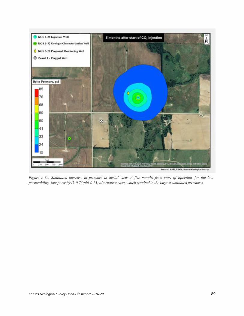
Figure A.3e. Simulated increase in pressure in aerial view at five months from start of injection for the low permeability–low porosity (k-0.75/phi-0.75) alternative case, which resulted in the largest simulated pressures.
Kansas Geological Survey Open-File Report 2016-29 90
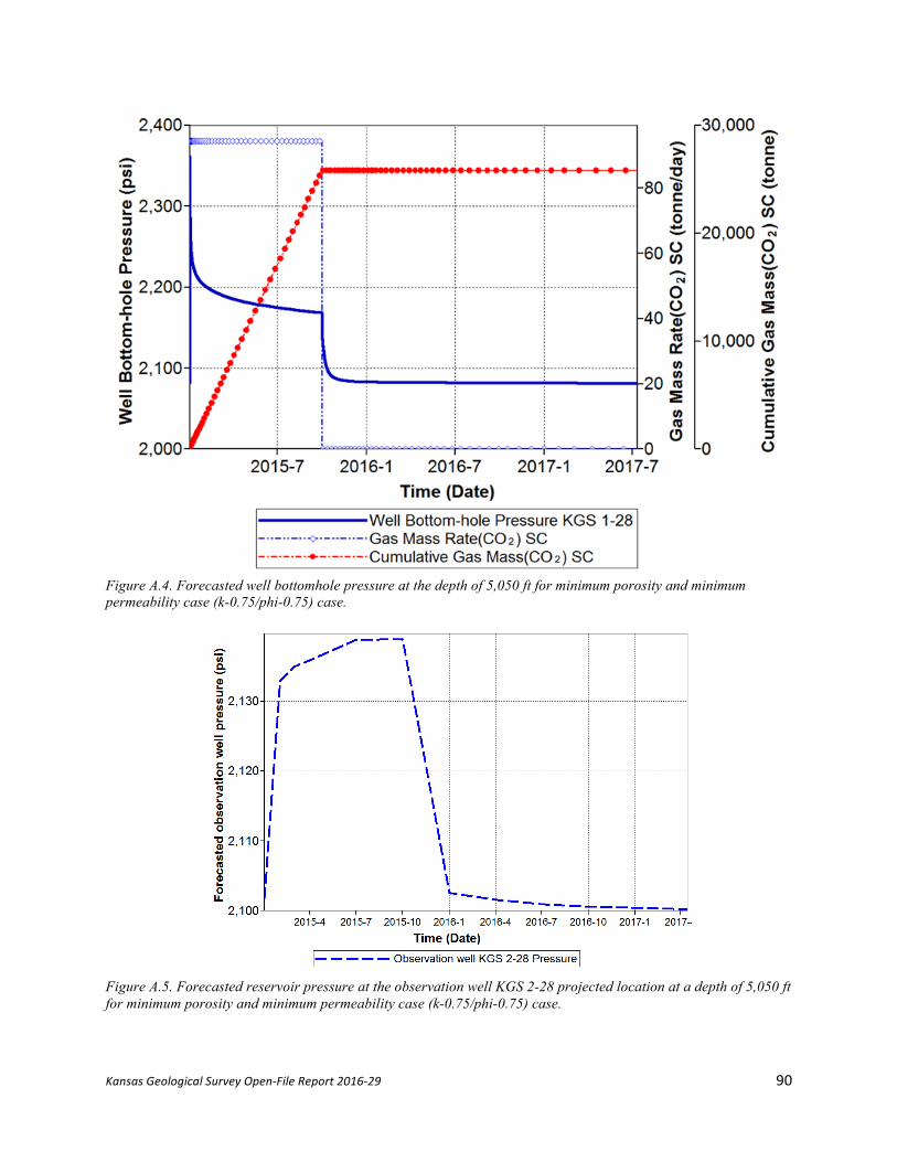
Figure A.4. Forecasted well bottomhole pressure at the depth of 5,050 ft for minimum porosity and minimum permeability case (k-0.75/phi-0.75) case.
Figure A.5. Forecasted reservoir pressure at the observation well KGS 2-28 projected location at a depth of 5,050 ft for minimum porosity and minimum permeability case (k-0.75/phi-0.75) case.

Kansas Geological Survey Open-File Report 2016-29 91
A2.Long-TermForecastforCO2Migrationforthe26,000tonsofCO2InjectionScenario
A2.1Long-TermFree-Phase Figure A.6a–f corresponds with fig. 14a–f in Section 6 of this report. They represent simulation results for an injection volume of 26,000 MT (compared to 40,000 MT in Section 6 simulations).
Kansas Geological Survey Open-File Report 2016-29 92
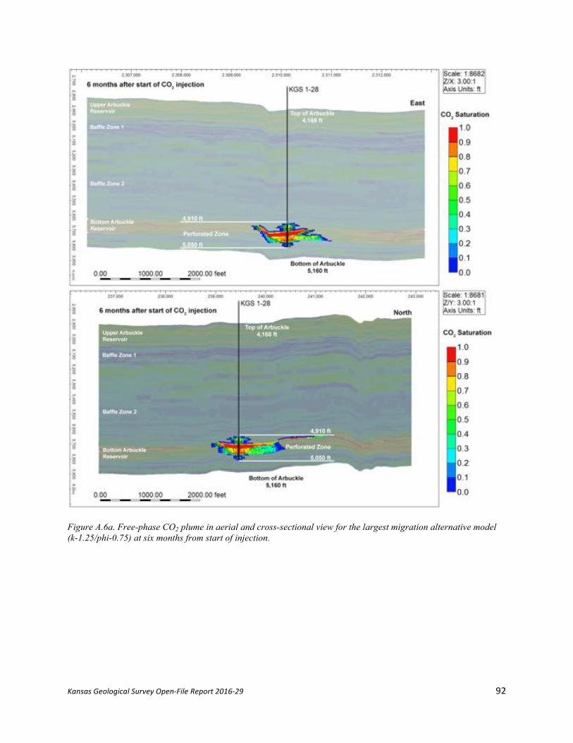
Figure A.6a. Free-phase CO2 plume in aerial and cross-sectional view for the largest migration alternative model (k-1.25/phi-0.75) at six months from start of injection.

Kansas Geological Survey Open-File Report 2016-29 93

Kansas Geological Survey Open-File Report 2016-29 94
Figure A.6b. Free-phase CO2 plume in aerial and cross-sectional view for the largest migration alternative model (k-1.25/phi-0.75) at nine months from start of injection. Injection stops at the end of this month.

Kansas Geological Survey Open-File Report 2016-29 95
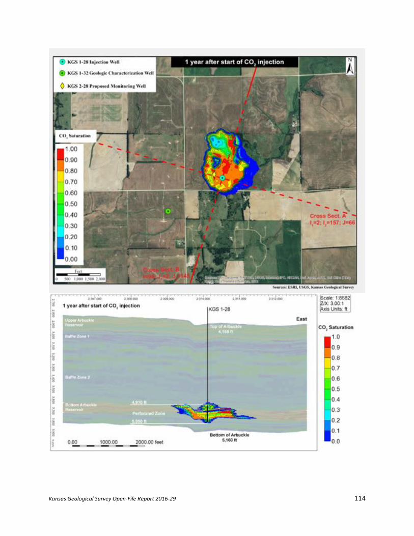
Figure A.6c. Free-phase CO2 plume in aerial and cross-sectional view for the largest migration alternative model (k-1.25/phi-0.75) at one year from start of injection.
Kansas Geological Survey Open-File Report 2016-29 96
Kansas Geological Survey Open-File Report 2016-29 97
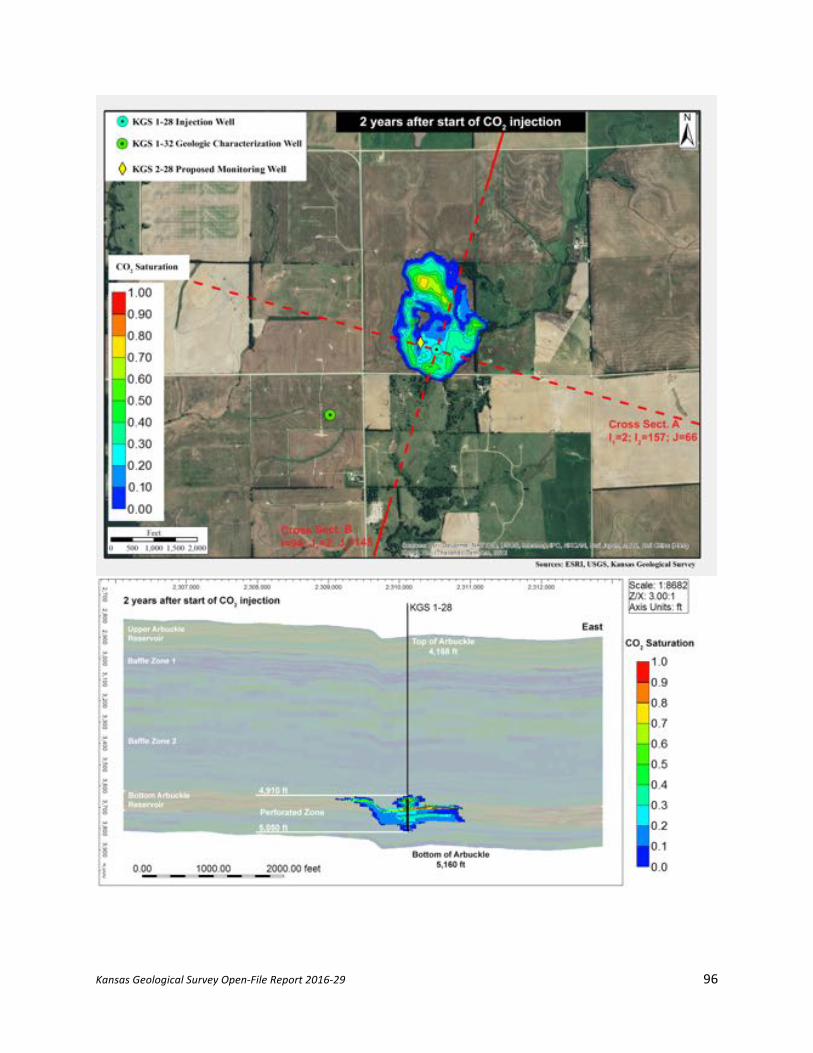
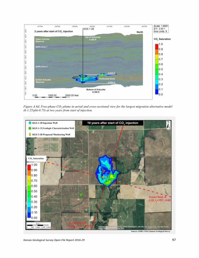
Figure A.6d. Free-phase CO2 plume in aerial and cross-sectional view for the largest migration alternative model (k-1.25/phi-0.75) at two years from start of injection.

Kansas Geological Survey Open-File Report 2016-29 98
Figure A.6e. Free-phase CO2 plume in aerial and cross-sectional view for the largest migration alternative model (k-1.25/phi-0.75) at 10 years from start of injection.
Kansas Geological Survey Open-File Report 2016-29 99
Kansas Geological Survey Open-File Report 2016-29 100
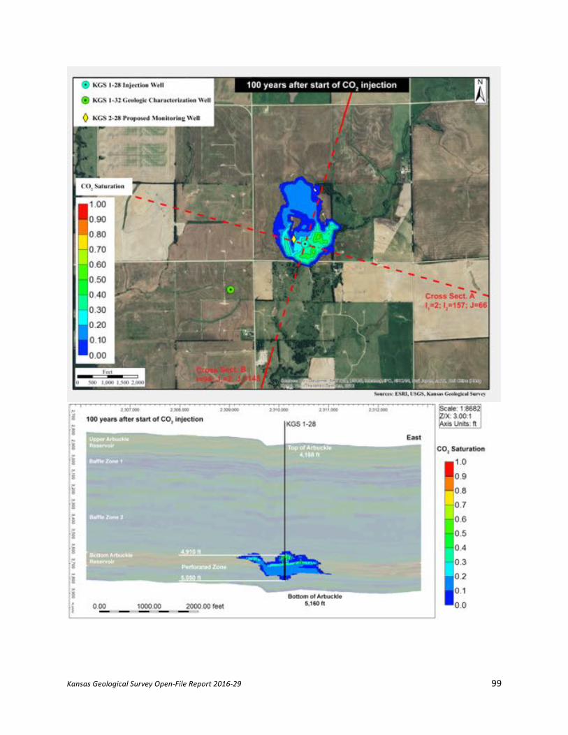
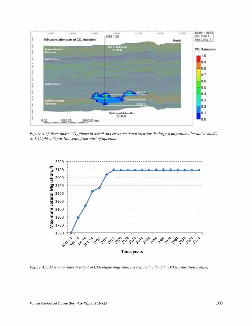
Figure A.6f. Free-phase CO2 plume in aerial and cross-sectional view for the largest migration alternative model (k-1.25/phi-0.75) at 100 years from start of injection.
Figure A.7. Maximum lateral extent of CO2 plume migration (as defined by the 0.5% CO2 saturation isoline).
1500
1700
1900
2100
2300
2500
2700
2900
3100
3300
Maxim
umLateralM
igra)o
n,2
Time,years
Kansas Geological Survey Open-File Report 2016-29 101
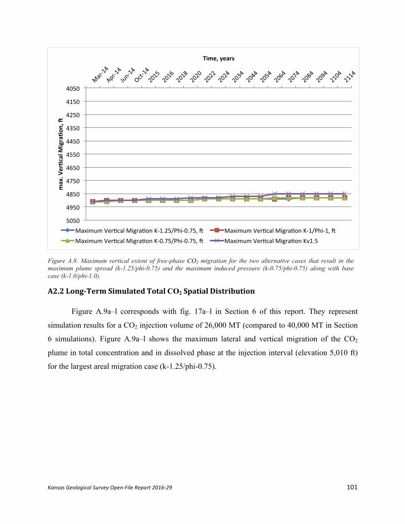
Figure A.8. Maximum vertical extent of free-phase CO2 migration for the two alternative cases that result in the maximum plume spread (k-1.25/phi-0.75) and the maximum induced pressure (k-0.75/phi-0.75) along with base case (k-1.0/phi-1.0).
A2.2Long-TermSimulatedTotalCO2SpatialDistribution
Figure A.9a–l corresponds with fig. 17a–l in Section 6 of this report. They represent
simulation results for a CO2 injection volume of 26,000 MT (compared to 40,000 MT in Section
6 simulations). Figure A.9a–l shows the maximum lateral and vertical migration of the CO2
plume in total concentration and in dissolved phase at the injection interval (elevation 5,010 ft)
for the largest areal migration case (k-1.25/phi-0.75).
4050
4150
4250
4350
4450
4550
4650
4750
4850
4950
5050
max.V
er)calM
igra)o
n,2
Time,years
MaximumVer5calMigra5onK-1.25/Phi-0.75,B MaximumVer5calMigra5onK-1/Phi-1,BMaximumVer5calMigra5onK-0.75/Phi-0.75,B MaximumVer5calMigra5onKv1.5

Kansas Geological Survey Open-File Report 2016-29 102

Kansas Geological Survey Open-File Report 2016-29 103
Figure A.9a. Total CO2 spatial distribution in aerial and cross-sectional view for the largest migration alternative model (k-1.25/phi-0.75) at six months from start of injection.

Kansas Geological Survey Open-File Report 2016-29 104
Figure A.9b. Total CO2 spatial distribution in aerial and cross-sectional view for the largest migration alternative model (k-1.25/phi-0.75) at nine months from start of injection. Injection stops at the end of this month.

Kansas Geological Survey Open-File Report 2016-29 105
Kansas Geological Survey Open-File Report 2016-29 106
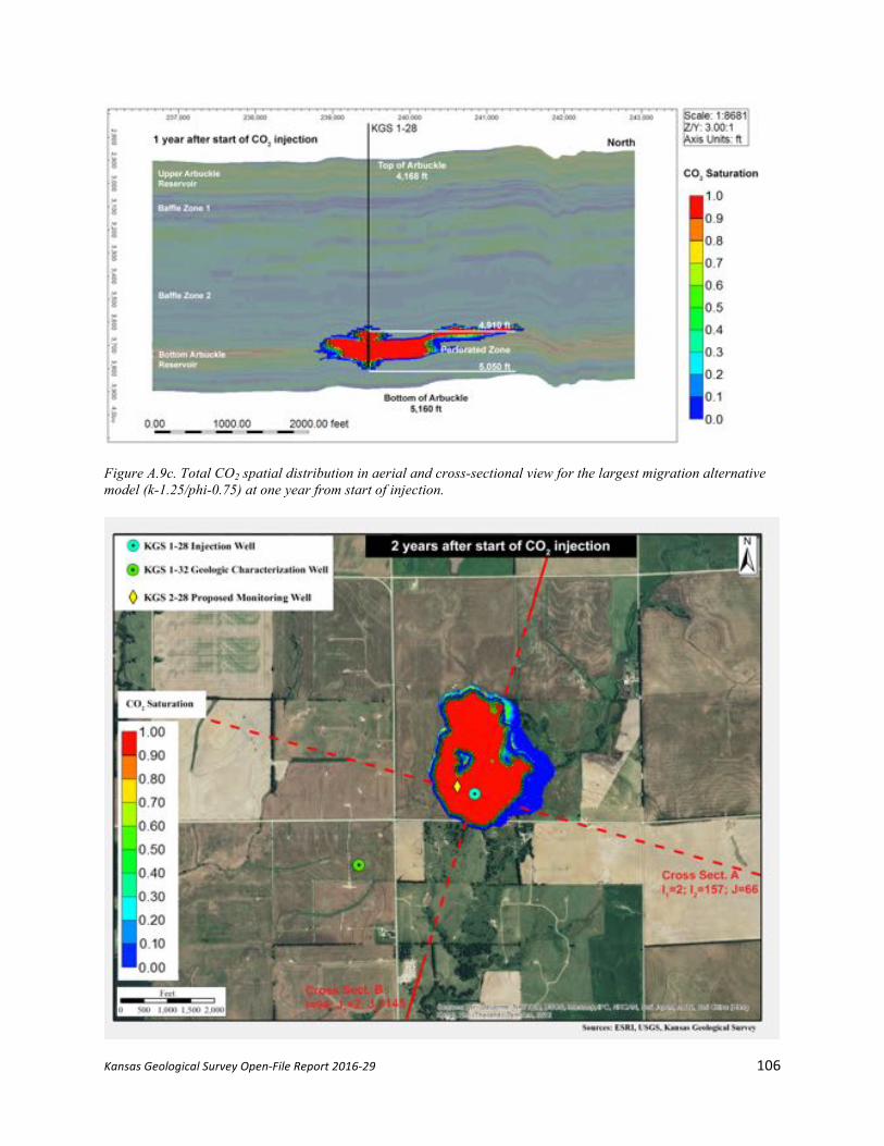
Figure A.9c. Total CO2 spatial distribution in aerial and cross-sectional view for the largest migration alternative model (k-1.25/phi-0.75) at one year from start of injection.
Kansas Geological Survey Open-File Report 2016-29 107
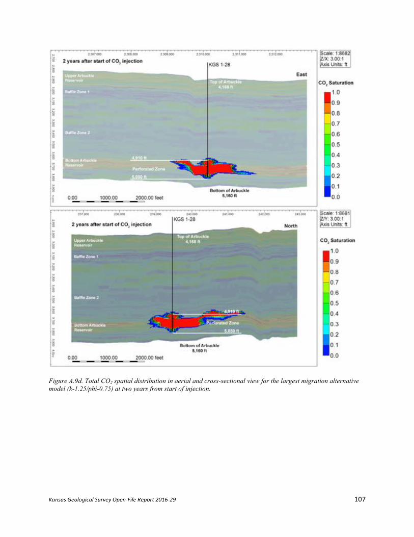
Figure A.9d. Total CO2 spatial distribution in aerial and cross-sectional view for the largest migration alternative model (k-1.25/phi-0.75) at two years from start of injection.
Kansas Geological Survey Open-File Report 2016-29 108
Kansas Geological Survey Open-File Report 2016-29 109
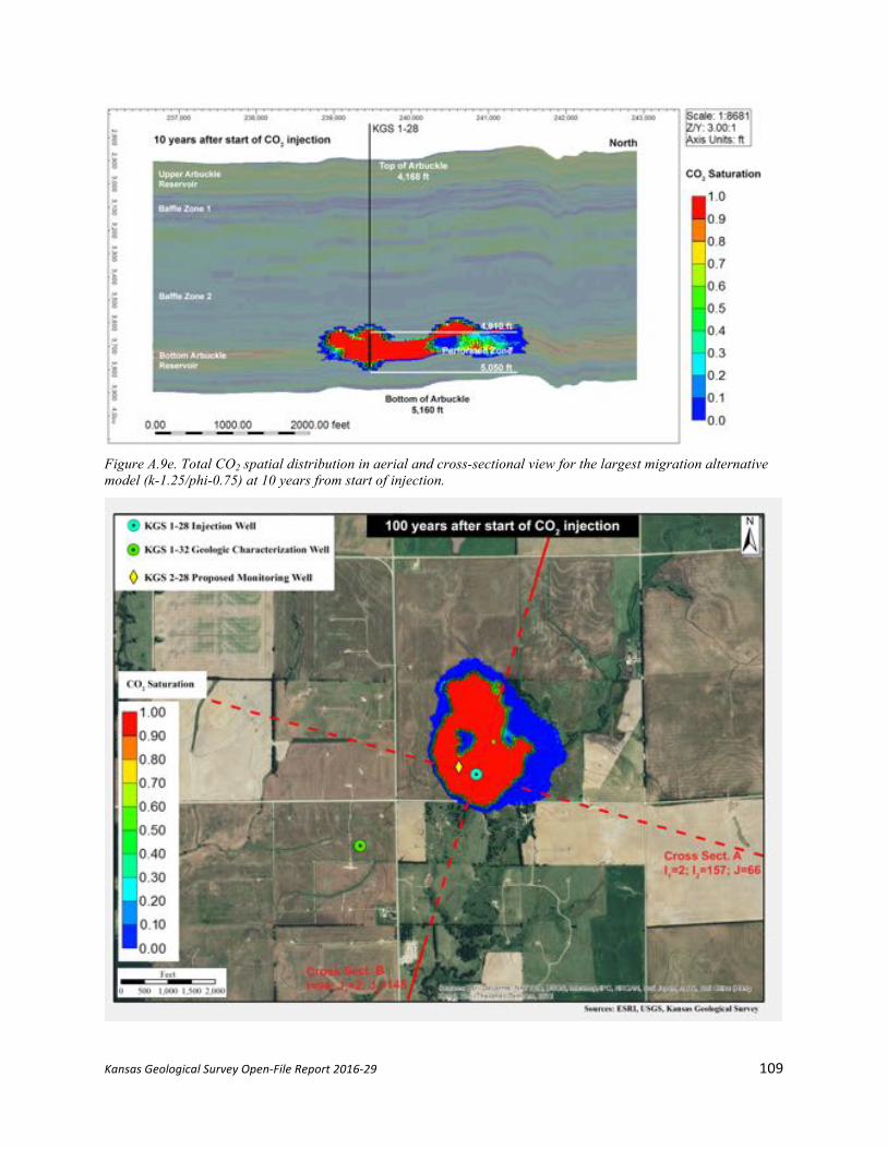
Figure A.9e. Total CO2 spatial distribution in aerial and cross-sectional view for the largest migration alternative model (k-1.25/phi-0.75) at 10 years from start of injection.

Kansas Geological Survey Open-File Report 2016-29 110
Figure A.9f. Total CO2 spatial distribution in aerial and cross-sectional view for the largest migration alternative model (k-1.25/phi-0.75) at 100 years from start of injection.

Kansas Geological Survey Open-File Report 2016-29 111

Kansas Geological Survey Open-File Report 2016-29 112
Figure A.9g. Dissolved CO2 spatial distribution in aerial and cross-sectional view for the largest migration alternative model (k-1.25/phi-0.75) at six months from start of injection.

Kansas Geological Survey Open-File Report 2016-29 113
Figure A.9h. Dissolved CO2 spatial distribution in aerial and cross-sectional view for the largest migration alternative model (k-1.25/phi-0.75) at nine months from start of injection. Injection stops at the end of this month.
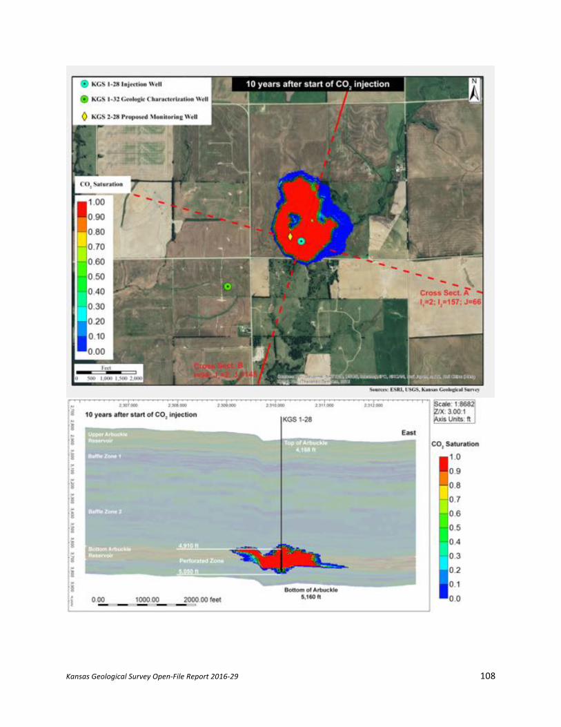
Kansas Geological Survey Open-File Report 2016-29 114

Kansas Geological Survey Open-File Report 2016-29 115
Figure A.9i. Dissolved CO2 spatial distribution in aerial and cross-sectional view for the largest migration alternative model (k-1.25/phi-0.75) at one year from start of injection.

Kansas Geological Survey Open-File Report 2016-29 116
Figure A.9j. Dissolved CO2 spatial distribution in aerial and cross-sectional view for the largest migration alternative model (k-1.25/phi-0.75) at two years from start of injection.

Kansas Geological Survey Open-File Report 2016-29 117
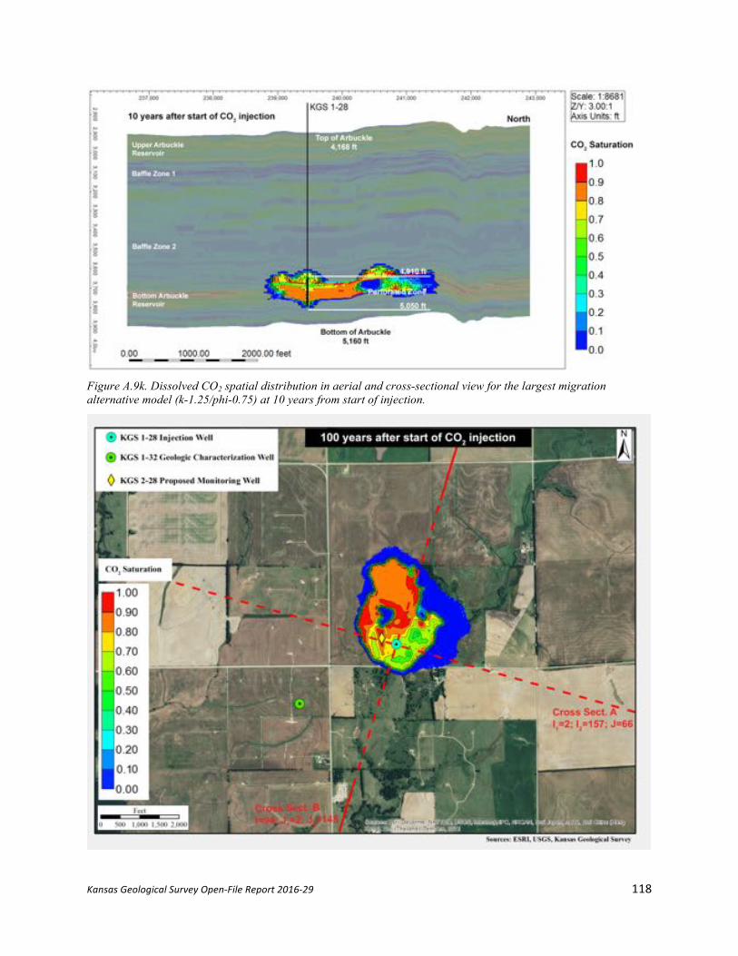
Kansas Geological Survey Open-File Report 2016-29 118
Figure A.9k. Dissolved CO2 spatial distribution in aerial and cross-sectional view for the largest migration alternative model (k-1.25/phi-0.75) at 10 years from start of injection.

Kansas Geological Survey Open-File Report 2016-29 119
Figure A.9l. Dissolved CO2 spatial distribution in aerial and cross-sectional view for the largest migration alternative model (k-1.25/phi-0.75) at 100 years from start of injection.
A2.3SimulatedPressureDistribution
Figure A.10 presents the bottomhole pressure (at a reference depth of 5,050 ft) for the
base case and the two cases that resulted in highest pressures and plume migration. The
bottomhole pressures for all nine alternative cases are listed in table 7. For all three cases
presented in fig. A.10, the pressure increases when CO2 injection operations start and then
drops to nearly pre-injection values when injection ceases. The pressure is influenced by

Kansas Geological Survey Open-File Report 2016-29 120
permeability and porosity, as these two parameters are independent (decoupled) variables in
CMG. Therefore, as expected, the highest bottomhole pressure (BHP) of 2,361 psi at a depth
of 5,050 ft is observed for the low permeability–low porosity case. This pressure represents an
increase of 268 psi over pre-injection levels and results in a pressure gradient of 0.467 psi/ft,
which is less than the maximum allowable pressure gradient of 0.675 psi/ft corresponding to
90% of the fracture gradient (0.75 psi/ft).
Figure A.10—Maximum well bottomhole pressure at a depth of 5,050 ft for minimum porosity and minimum permeability (k-0.75/phi-0.75) case.
Figure A.11 presents the change in pore pressure at the base of the confining zone
(Simpson Group) for the case that resulted in the highest pressures and plume spread. The
maximum pressure increase at the end of the injection period is fairly small and varies between
0.7 psi and 0.8 psi. As observed for pressures at the bottom of the well, the highest pressure is
noted for the low permeability/low porosity case (k-0.75/phi-0.75).
Figure A.13a–e presents the lateral distribution of pressure in the Arbuckle injection
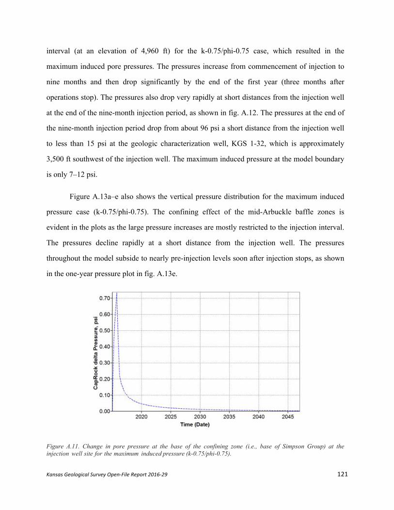
Kansas Geological Survey Open-File Report 2016-29 121
interval (at an elevation of 4,960 ft) for the k-0.75/phi-0.75 case, which resulted in the
maximum induced pore pressures. The pressures increase from commencement of injection to
nine months and then drop significantly by the end of the first year (three months after
operations stop). The pressures also drop very rapidly at short distances from the injection well
at the end of the nine-month injection period, as shown in fig. A.12. The pressures at the end of
the nine-month injection period drop from about 96 psi a short distance from the injection well
to less than 15 psi at the geologic characterization well, KGS 1-32, which is approximately
3,500 ft southwest of the injection well. The maximum induced pressure at the model boundary
is only 7–12 psi.
Figure A.13a–e also shows the vertical pressure distribution for the maximum induced
pressure case (k-0.75/phi-0.75). The confining effect of the mid-Arbuckle baffle zones is
evident in the plots as the large pressure increases are mostly restricted to the injection interval.
The pressures decline rapidly at a short distance from the injection well. The pressures
throughout the model subside to nearly pre-injection levels soon after injection stops, as shown
in the one-year pressure plot in fig. A.13e.
Figure A.11. Change in pore pressure at the base of the confining zone (i.e., base of Simpson Group) at the injection well site for the maximum induced pressure (k-0.75/phi-0.75).

Kansas Geological Survey Open-File Report 2016-29 122
Figure A.12. Pore pressure as a function of lateral distance from the injection well (KGS 1-28) at seven time intervals for the highest induced pressure case (k-0.75/phi-0.75).

Kansas Geological Survey Open-File Report 2016-29 123
Figure A.13a. Simulated increase in pressure in aerial and cross-sectional views at one month from start of injection for the low permeability–low porosity (k-0.75/phi-0.75) alternative case, which resulted in the largest simulated pressures.
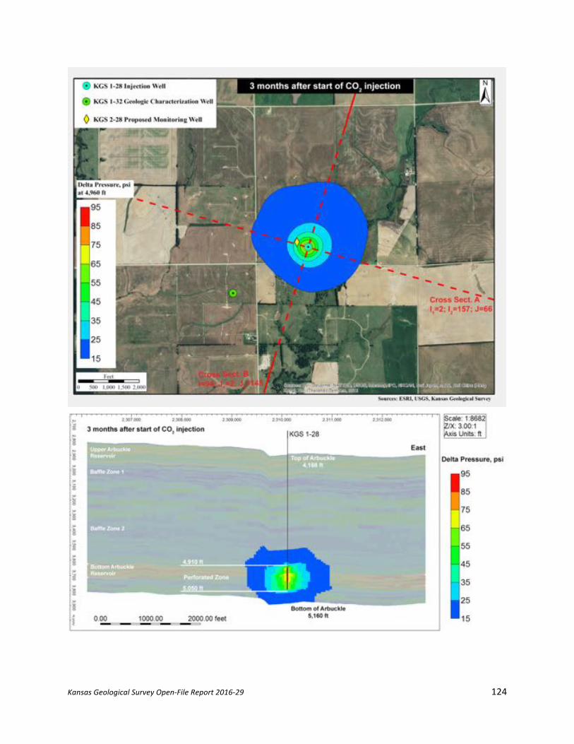
Kansas Geological Survey Open-File Report 2016-29 124
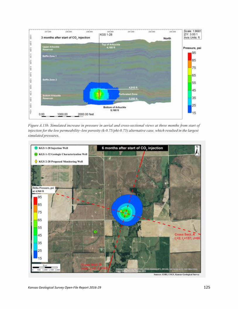
Kansas Geological Survey Open-File Report 2016-29 125
Figure A.13b. Simulated increase in pressure in aerial and cross-sectional views at three months from start of injection for the low permeability–low porosity (k-0.75/phi-0.75) alternative case, which resulted in the largest simulated pressures.

Kansas Geological Survey Open-File Report 2016-29 126
Figure A.13c. Simulated increase in pressure in aerial and cross-sectional views at six months from start of injection for the low permeability–low porosity (k-0.75/phi-0.75) alternative case, which resulted in the largest simulated pressures.

Kansas Geological Survey Open-File Report 2016-29 127
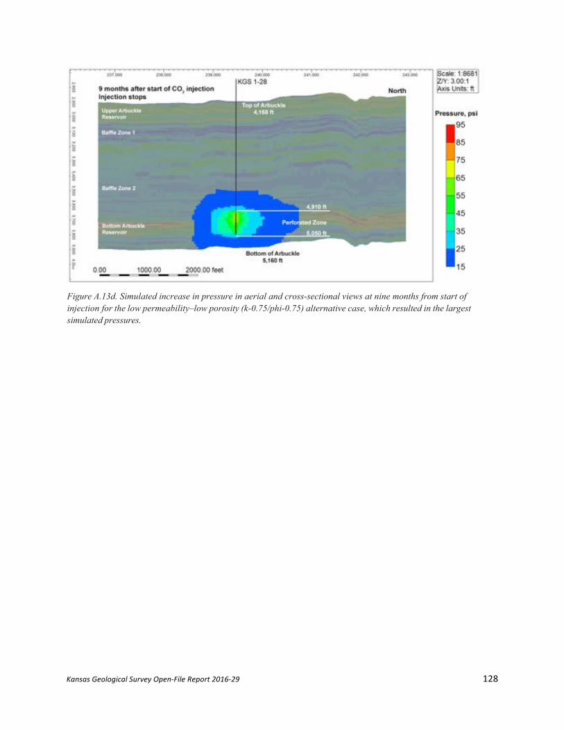
Kansas Geological Survey Open-File Report 2016-29 128
Figure A.13d. Simulated increase in pressure in aerial and cross-sectional views at nine months from start of injection for the low permeability–low porosity (k-0.75/phi-0.75) alternative case, which resulted in the largest simulated pressures.

Kansas Geological Survey Open-File Report 2016-29 129
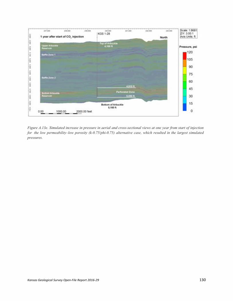
Kansas Geological Survey Open-File Report 2016-29 130
Figure A.13e. Simulated increase in pressure in aerial and cross-sectional views at one year from start of injection for the low permeability–low porosity (k-0.75/phi-0.75) alternative case, which resulted in the largest simulated pressures.

Kansas Geological Survey Open-File Report 2016-29 131
Appendix B. Capillary Pressure and Relative Permeability Drainage and Imbibition Tables for 9 Rock Types
Table B.1. RQI vs. rock type assignments.
RT RQI from RQI To Ave RQI
1 40 10 25 2 10 2.5 6.25 3 2.5 1 1.75 4 1 0.5 0.75 5 0.5 0.4 0.45 6 0.4 0.3 0.35 7 0.3 0.2 0.25 8 0.2 0.1 0.15
9 0.1 0.01 0.055
Table B.2. Capillary pressure and relative permeability drainage and imbibition tables for rock type 1 (RQI=25).
RQI range from 40-10- Ave RQI =25
RQI range from 40-10- Ave RQI =25
Pc Sw SCO2 Krw krCO2
Pc Sw SCO2 Krw krCO2
0 1 0 1 0
0 0.652 0.348 0.075032 0.0000 0.012 0.933 0.0666 0.8758 0.0000
0.005 0.4689 0.5311 0.027558 0.0184
0.015 0.765 0.2348 0.5973 0.0011
0.01 0.3693 0.6307 0.013298 0.0650 0.018 0.651 0.3494 0.4368 0.0065
0.02 0.2627 0.7373 0.004674 0.1645
0.02 0.593 0.4075 0.3646 0.0129
0.03 0.2060 0.7940 0.002204 0.2440 0.03 0.414 0.5862 0.1818 0.0664
0.04 0.1706 0.8294 0.001225 0.3045
0.04 0.321 0.6789 0.1110 0.1285
0.05 0.1463 0.8537 0.000756 0.3512 0.05 0.264 0.7360 0.0757 0.1848
0.06 0.1285 0.8715 0.000502 0.3882
0.06 0.225 0.7748 0.0553 0.2329
0.07 0.1150 0.8850 0.000352 0.4181 0.07 0.197 0.8031 0.0425 0.2736
0.08 0.1042 0.8958 0.000257 0.4428
0.08 0.175 0.8246 0.0338 0.3081
0.09 0.0955 0.9045 0.000194 0.4635 0.09 0.158 0.8415 0.0276 0.3377
0.1 0.0883 0.9117 0.00015 0.4812
0.1 0.145 0.8552 0.0230 0.3631
0.2 0.0525 0.9475 2.64E-05 0.5751 0.15 0.103 0.8974 0.0115 0.4509
0.3 0.0391 0.9609 9.21E-06 0.6135
0.2 0.081 0.9192 0.0070 0.5024
0.4 0.0319 0.9681 4.31E-06 0.6345 0.3 0.058 0.9418 0.0035 0.5605
0.5 0.0274 0.9726 2.38E-06 0.6479
0.4 0.046 0.9535 0.0021 0.5926
0.6 0.0243 0.9757 1.46E-06 0.6572 0.5 0.039 0.9608 0.0014 0.6131
0.7 0.0221 0.9779 9.6E-07 0.6641
0.6 0.034 0.9657 0.0010 0.6273
0.8 0.0204 0.9796 6.68E-07 0.6693 0.7 0.031 0.9693 0.0008 0.6379
0.9 0.0190 0.9810 4.84E-07 0.6735
0.8 0.028 0.9720 0.0006 0.6459
1 0.0179 0.9821 3.63E-07 0.6769 0.9 0.026 0.9741 0.0005 0.6524
2 0.0127 0.9873 5.25E-08 0.6931

Kansas Geological Survey Open-File Report 2016-29 132
1 0.024 0.9759 0.0004 0.6576
3 0.0109 0.9891 1.64E-08 0.6989 1.5 0.019 0.9812 0.0002 0.6740
4 0.0099 0.9901 6.99E-09 0.7019
2 0.016 0.9840 0.0001 0.6825
5 0.0093 0.9907 3.55E-09 0.7038 3 0.013 0.9868 0.0001 0.6915
6 0.0089 0.9911 2.01E-09 0.7051
4 0.012 0.9883 3.62E-05 0.6962
7 0.0086 0.9914 1.23E-09 0.7060 5 0.011 0.9892 2.40E-05 0.6991
8 0.0084 0.9916 7.91E-10 0.7067
6 0.010 0.9898 1.70E-05 0.7011
9 0.0082 0.9918 5.31E-10 0.7073 7 0.010 0.9903 1.27E-05 0.7025
10 0.0081 0.9919 3.68E-10 0.7077
8 0.009 0.9906 9.76E-06 0.7036
12 0.0079 0.9921 1.9E-10 0.7084 9 0.009 0.9909 7.73E-06 0.7045
14 0.0077 0.9923 1.05E-10 0.7089
10 0.009 0.9911 6.26E-06 0.7052
20 0.0074 0.9926 0 0.7112 12 0.009 0.9915 4.30E-06 0.7063
30 0.0072 0.9928 0 0.7112
14 0.008 0.9917 3.10E-06 0.7071
40 0.0071 0.9929 0 0.7112 18 0.008 0.9920 1.77E-06 0.7081
50 0.0070 0.9930 0 0.7112
20 0.008 0.9922 1.38E-06 0.7085
60 0.0069 0.9931 0 0.7112 25 0.008 0.9924 7.86E-07 0.7092
70 0.0069 0.9931 0 0.7112
30 0.007 0.9925 4.75E-07 0.7097
80 0.0069 0.9931 0 0.7112 40 0.007 0.9927 1.87E-07 0.7103
90 0.0069 0.9931 0 0.7112
50 0.007 0.00 0.00 0.7112
100 0.0068 0.9932 0 0.7112 60 0.007 0.00 0.00 0.7112
150 0.0068 0.9932 0 0.7112
70 0.007 0.00 0.00 0.7112
200 0.0068 0.9932 0 0.7112
80 0.007 0.00 0.00 0.7112
300 0.0067 0.9933 0 0.7112
90 0.007 0.00 0.00 0.7112 100 0.007 0.00 0.00 0.7112 150 0.007 0.00 0.00 0.7112 200 0.007 0.00 0.00 0.7112 300 0.007 0.00 0.00 0.7112
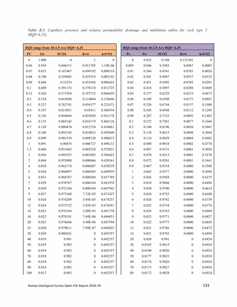
Kansas Geological Survey Open-File Report 2016-29 133
Table B.3. Capillary pressure and relative permeability drainage and imbibition tables for rock type 2 (RQI=6.25).
RQI range from 10-2.5-Ave RQI= 6.25
RQI range from 10-2.5-Ave RQI= 6.25
PC Sw SCO2 Krw krCO2
Pc Sw SCO2 Krw krCO2
0 1.000 0 1 0
0 0.652 0.348 0.121501 0 0.06 0.954 0.046311 0.911705 1.19E-06
0.005 0.606 0.3943 0.0967 0.0005
0.07 0.833 0.167467 0.699192 0.000318
0.01 0.566 0.4341 0.0783 0.0026 0.08 0.740 0.259685 0.555519 0.002142
0.02 0.501 0.4987 0.0537 0.0125
0.09 0.668 0.33234 0.453456 0.006265
0.03 0.451 0.5492 0.0385 0.0281 0.1 0.609 0.391133 0.378118 0.012725
0.04 0.410 0.5897 0.0286 0.0469
0.15 0.428 0.571954 0.187715 0.066459
0.05 0.377 0.6229 0.0219 0.0673 0.2 0.334 0.665688 0.114064 0.128606
0.06 0.349 0.6508 0.0172 0.0881
0.3 0.237 0.762741 0.056377 0.232473
0.07 0.326 0.6744 0.0137 0.1088 0.4 0.187 0.813051 0.03411 0.306934
0.08 0.305 0.6948 0.0112 0.1289
0.5 0.156 0.844044 0.023058 0.361178
0.09 0.287 0.7125 0.0092 0.1482 0.6 0.135 0.865142 0.016719 0.402126
0.1 0.272 0.7281 0.0077 0.1666
0.7 0.120 0.880474 0.012724 0.434061
0.2 0.180 0.8196 0.0020 0.3047 0.8 0.108 0.892145 0.010033 0.459649
0.3 0.138 0.8615 0.0008 0.3868
0.9 0.099 0.901339 0.008128 0.480615
0.4 0.114 0.8859 0.0004 0.4403 1 0.091 0.90878 0.006727 0.498113
0.5 0.098 0.9018 0.0002 0.4778
1.5 0.068 0.931663 0.003218 0.555021
0.6 0.087 0.9131 0.0001 0.5056 2 0.056 0.943525 0.001885 0.586423
0.7 0.078 0.9215 0.0001 0.5270
3 0.044 0.955808 0.000866 0.620361
0.8 0.072 0.9281 0.0001 0.5441 4 0.038 0.962174 0.000487 0.638539
0.9 0.067 0.9334 0.0000 0.5580
5 0.034 0.966097 0.000305 0.649939
1 0.062 0.9377 0.0000 0.5696 6 0.031 0.968767 0.000204 0.657789
2 0.042 0.9584 0.0000 0.6275
7 0.029 0.970707 0.000144 0.663539
3 0.034 0.9660 0.0000 0.6496 8 0.028 0.972184 0.000104 0.667942
4 0.030 0.9700 0.0000 0.6614
9 0.027 0.973348 7.73E-05 0.671427
5 0.028 0.9725 0.0000 0.6688 10 0.026 0.974289 5.84E-05 0.674257
6 0.026 0.9742 0.0000 0.6739
12 0.024 0.975722 3.45E-05 0.678581
7 0.025 0.9754 0.0000 0.6776 14 0.023 0.976764 2.09E-05 0.681738
8 0.024 0.9763 0.0000 0.6804
18 0.022 0.978181 7.69E-06 0.686051
9 0.023 0.9771 0.0000 0.6827 20 0.021 0.978686 4.49E-06 0.687594
10 0.022 0.9777 0.0000 0.6845
25 0.020 0.979611 7.99E-07 0.690425
12 0.021 0.9786 0.0000 0.6873 30 0.020 0.980241 0 0.692357
14 0.021 0.9793 0.0000 0.6894
40 0.019 0.981 0 0.692357
20 0.020 0.981 0 0.6924 50 0.018 0.982 0 0.692357
30 0.0185 0.9815 0 0.6924
60 0.018 0.982 0 0.692357
40 0.0180 0.9820 0 0.6924 70 0.018 0.982 0 0.692357
50 0.0177 0.9823 0 0.6924
80 0.018 0.982 0 0.692357
60 0.0174 0.9826 0 0.6924 90 0.018 0.982 0 0.692357
70 0.0173 0.9827 0 0.6924
100 0.017 0.983 0 0.692357
80 0.0172 0.9828 0 0.6924

Kansas Geological Survey Open-File Report 2016-29 134
150 0.017 0.983 0 0.692357
90 0.0171 0.9829 0 0.6924 200 0.017 0.983 0 0.692357
100 0.0170 0.9830 0 0.6924
300 0.017 0.983 0 0.692357
150 0.0168 0.9832 0 0.6924
200 0.0166 0.9834 0 0.6924
300 0.0165 0.9835 0 0.6924

Kansas Geological Survey Open-File Report 2016-29 135
Table B.4. Capillary pressure and relative permeability drainage and imbibition tables for rock type 3 (RQI=1.75).
RQI range from 2.5-1 -Ave RQI=1.75
RQI range from 2.5-1 -Ave RQI=1.75
Pc Sw SCO2 Krw krCO2
Pc Sw SCO2 Krw krCO2
0 1.000 0 1 0
0 0.654 0.346 0.189511 0 0.3 0.868 0.131574 0.752199 0.000167
0.005 0.643 0.356679 0.179635 1.18E-05
0.4 0.679 0.320874 0.45511 0.007077
0.01 0.633 0.366974 0.170445 7.54E-05 0.5 0.563 0.437491 0.307641 0.026021
0.02 0.614 0.386496 0.153889 0.000452
0.6 0.483 0.516876 0.223065 0.052417
0.03 0.595 0.404715 0.139439 0.001237 0.7 0.425 0.574567 0.169764 0.081749
0.04 0.578 0.421759 0.126767 0.002468
0.8 0.382 0.618479 0.13386 0.111382
0.05 0.562 0.437739 0.115606 0.004143 0.9 0.347 0.653076 0.108447 0.13999
0.06 0.547 0.452754 0.105734 0.006245
1 0.319 0.681071 0.089755 0.166978
0.07 0.533 0.46689 0.09697 0.008742 1.5 0.233 0.767174 0.042942 0.275299
0.08 0.520 0.480224 0.08916 0.011601
2 0.188 0.811808 0.025156 0.349104
0.09 0.507 0.492822 0.082176 0.014787 3 0.142 0.858022 0.011556 0.440498
0.1 0.495 0.504746 0.075912 0.018263
4 0.118 0.881978 0.006492 0.494509
0.2 0.404 0.596381 0.038024 0.062589 5 0.103 0.896736 0.004068 0.530205
0.3 0.344 0.656344 0.021774 0.111804
6 0.093 0.906783 0.002728 0.555603
0.4 0.301 0.698778 0.013632 0.158065 7 0.086 0.914084 0.001915 0.574635
0.5 0.270 0.730464 0.009096 0.199413
8 0.080 0.919641 0.001388 0.589451
0.6 0.245 0.755069 0.006367 0.235796 9 0.076 0.924019 0.001031 0.601328
0.7 0.225 0.774756 0.004626 0.267721
10 0.072 0.927562 0.000779 0.611071
0.8 0.209 0.790883 0.003463 0.295801 12 0.067 0.932954 0.00046 0.62613
0.9 0.196 0.804346 0.002656 0.32061
14 0.063 0.936873 0.000279 0.63725
1 0.184 0.815765 0.002079 0.342646 18 0.058 0.942205 0.000103 0.652624
2 0.124 0.876117 0.000346 0.474936
20 0.056 0.944107 5.99E-05 0.658174
3 0.099 0.900586 0.000104 0.5365 25 0.052 0.947587 1.07E-05 0.668423
4 0.086 0.913988 4E-05 0.572243
30 0.050 0.949955 0 0.675469
5 0.078 0.922497 1.78E-05 0.595694 40 0.047 0.050045 0 0.675469
6 0.072 0.928401 8.61E-06 0.612315
50 0.045 0.949955 0 0.675469
7 0.067 0.932748 4.38E-06 0.62474 60 0.044 0.050045 0 0.675469
8 0.064 0.93609 2.29E-06 0.634396
70 0.043 0.949955 0 0.675469
9 0.061 0.938742 1.21E-06 0.642127 80 0.042 0.050045 0 0.675469
10 0.059 0.940901 6.39E-07 0.648464
90 0.042 0.949955 0 0.675469
12 0.056 0.944208 1.63E-07 0.658247 100 0.041 0.050045 0 0.675469
14 0.053 0.946628 3.17E-08 0.665464
150 0.040 0.949955 0 0.675469
20 0.0489 0.9511 0 0.675469 200 0.039 0.050045 0 0.675469
30 0.0452 0.9548 0 0.675469
300 0.038 0.949955 0 0.675469
40 0.0433 0.9567 0 0.675469
50 0.0421 0.9579 0 0.675469
60 0.0413 0.9587 0 0.675469
70 0.0407 0.9593 0 0.675469
80 0.0403 0.9597 0 0.675469

Kansas Geological Survey Open-File Report 2016-29 136
90 0.0399 0.9601 0 0.675469
100 0.0396 0.9604 0 0.675469
150 0.0387 0.9613 0 0.675469
200 0.0383 0.9617 0 0.675469
300 0.0378 0.9622 0 0.675469

Kansas Geological Survey Open-File Report 2016-29 137
Table B.5. Capillary pressure and relative permeability drainage and imbibition tables for rock type 4 (RQI=0.75).
RQI range from1-0.5-Ave RQI=0.75
RQI range from1-0.5-Ave RQI=0.75
Pc Sw SCO2 Krw krCO2
Pc Sw SCO2 Krw krCO2
0 1.000 0 1 0
0 0.657 0.3426 0.254272 0 0.7 0.989 0.010684 0.977573 1.03E-08
0.005 0.653 0.34683 0.248578 1.95E-06
0.8 0.885 0.115298 0.770825 0.000158
0.01 0.649 0.350608 0.243564 1.04E-05 0.9 0.802 0.19772 0.624483 0.001403
0.02 0.642 0.358013 0.233934 5.73E-05
1 0.736 0.264415 0.516846 0.004553
0.03 0.635 0.365222 0.224805 0.000156 1.5 0.530 0.469544 0.247276 0.046594
0.04 0.628 0.372245 0.216145 0.000315
2 0.424 0.575878 0.14486 0.106509
0.05 0.621 0.379087 0.207923 0.00054 3 0.314 0.685977 0.066547 0.216321
0.06 0.614 0.385757 0.200112 0.000837
4 0.257 0.74305 0.037386 0.298998
0.07 0.608 0.39226 0.192687 0.001205 5 0.222 0.778209 0.023425 0.360567
0.08 0.601 0.398603 0.185624 0.001648
6 0.198 0.802143 0.015709 0.40763
0.09 0.595 0.404792 0.178902 0.002165 7 0.180 0.819537 0.011027 0.444629
0.1 0.589 0.410832 0.172499 0.002755
8 0.167 0.832776 0.007996 0.474444
0.2 0.536 0.464129 0.122488 0.012366 9 0.157 0.843207 0.005936 0.498975
0.3 0.493 0.507166 0.090005 0.027205
10 0.148 0.851647 0.004484 0.519515
0.4 0.457 0.542681 0.067988 0.045221 12 0.136 0.864493 0.002649 0.551989
0.5 0.427 0.572511 0.05254 0.064908
14 0.126 0.873829 0.001606 0.576531
0.6 0.402 0.597939 0.041384 0.085264 18 0.113 0.886533 0.000591 0.611239
0.7 0.380 0.619885 0.033129 0.105653
20 0.109 0.891064 0.000345 0.623988
0.8 0.361 0.639028 0.026894 0.125682 25 0.101 0.899354 6.14E-05 0.647835
0.9 0.344 0.65588 0.022099 0.145117
30 0.095 0.904997 0 0.664456
1 0.329 0.670835 0.018353 0.163825 40 0.088 0.912 0 0.664456
2 0.238 0.76151 0.004223 0.308916
50 0.083 0.917 0 0.664456
3 0.195 0.804785 0.001439 0.398896 60 0.080 0.920 0 0.664456
4 0.170 0.830335 0.000595 0.458797
70 0.078 0.922 0 0.664456
5 0.153 0.847279 0.000275 0.501402 80 0.076 0.924 0 0.664456
6 0.141 0.859378 0.000136 0.533259
90 0.075 0.925 0 0.664456
7 0.132 0.86847 6.97E-05 0.557999 100 0.074 0.926 0 0.664456
8 0.124 0.875564 3.64E-05 0.577784
150 0.071 0.929 0 0.664456
9 0.119 0.881261 1.91E-05 0.593981 200 0.069 0.931 0 0.664456
10 0.114 0.885942 9.89E-06 0.607495
300 0.067 0.933 0 0.664456
12 0.107 0.893189 2.35E-06 0.628788
14 0.101 0.898549 3.83E-07 0.64483
20 0.091345 0.908655 0 0.664456
30 0.082976 0.917024 0 0.664456
40 0.078568 0.921432 0 0.664456
50 0.075829 0.924171 0 0.664456
60 0.073955 0.926045 0 0.664456
70 0.072588 0.927412 0 0.664456
80 0.071544 0.928456 0 0.664456

Kansas Geological Survey Open-File Report 2016-29 138
90 0.07072 0.92928 0 0.664456
100 0.070052 0.929948 0 0.664456
150 0.067993 0.932007 0 0.664456
200 0.066922 0.933078 0 0.664456
300 0.06581 0.93419 0 0.664456

Kansas Geological Survey Open-File Report 2016-29 139
Table B.6. Capillary pressure and relative permeability drainage and imbibition tables for rock type 5 (RQI=0.45).
RQI range from 0.5-0.4 -AveRQI=0.45
RQI range from 0.5-0.4 -AveRQI=0.45
Pc Sw SCO2 Krw krCO2
Pc Sw SCO2 Krw krCO2
0 1.000 0 1 0
0 0.662 0.3376 0.303762 0 1.5 0.869 0.13133 0.728436 0.000433
0.005 0.660 0.340035 0.299527 9.31E-07
2 0.691 0.309055 0.426733 0.012203
0.01 0.658 0.342056 0.296043 4.32E-06 3 0.507 0.493071 0.196037 0.075452
0.02 0.654 0.346051 0.289234 2.17E-05
4 0.412 0.588461 0.110132 0.150391
0.03 0.650 0.349988 0.282627 5.66E-05 5 0.353 0.647226 0.069006 0.217992
0.04 0.646 0.353867 0.276216 0.000112
6 0.313 0.687229 0.046276 0.275433
0.05 0.642 0.35769 0.269993 0.00019 7 0.284 0.7163 0.032485 0.323737
0.06 0.639 0.361458 0.263952 0.000293
8 0.262 0.738428 0.023554 0.364521
0.07 0.635 0.365173 0.258086 0.000421 9 0.244 0.755861 0.017485 0.399251
0.08 0.631 0.368835 0.252388 0.000575
10 0.230 0.769968 0.013208 0.429108
0.09 0.628 0.372445 0.246854 0.000757 12 0.209 0.791439 0.007804 0.477694
0.1 0.624 0.376005 0.241476 0.000965
14 0.193 0.807042 0.004731 0.515487
0.2 0.591 0.409058 0.195229 0.004565 18 0.172 0.828276 0.00174 0.570433
0.3 0.562 0.43808 0.159845 0.010708
20 0.164 0.835848 0.001017 0.591042
0.4 0.536 0.463776 0.13233 0.018927 25 0.150 0.849704 0.000181 0.630181
0.5 0.513 0.486696 0.110624 0.028732
30 0.141 0.859136 0 0.657904
0.6 0.493 0.507273 0.093283 0.039698 40 0.129 0.871 0 0.657904
0.7 0.474 0.525854 0.079272 0.051479
50 0.121 0.879 0 0.657904
0.8 0.457 0.542719 0.067836 0.063798 60 0.116 0.884 0 0.657904
0.9 0.442 0.558101 0.058416 0.076443
70 0.113 0.887 0 0.657904
1 0.428 0.572188 0.050593 0.089247 80 0.110 0.890 0 0.657904
2 0.333 0.667435 0.015085 0.209236
90 0.108 0.892 0 0.657904
3 0.280 0.719672 0.005809 0.302188 100 0.106 0.894 0 0.657904
4 0.247 0.752861 0.00257 0.37216
150 0.100 0.900 0 0.657904
5 0.224 0.775901 0.001235 0.425955 200 0.097 0.903 0 0.657904
6 0.207 0.792873 0.000623 0.468401
300 0.095 0.905 0 0.657904
7 0.194 0.805921 0.000323 0.50269
8 0.184 0.816279 0.000169 0.530952
9 0.175 0.824712 8.73E-05 0.554649
10 0.168 0.831717 4.41E-05 0.574807
12 0.157 0.842699 9.51E-06 0.607283
14 0.149 0.85093 1.18E-06 0.632329
20 0.133303 0.866697 0 0.657904
30 0.119999 0.880001 0 0.657904
40 0.112904 0.887096 0 0.657904
50 0.108465 0.891535 0 0.657904
60 0.105413 0.894587 0 0.657904
70 0.103181 0.896819 0 0.657904
80 0.101474 0.898526 0 0.657904
90 0.100123 0.899877 0 0.657904

Kansas Geological Survey Open-File Report 2016-29 140
100 0.099027 0.900973 0 0.657904
150 0.095639 0.904361 0 0.657904
200 0.093872 0.906128 0 0.657904
300 0.092035 0.907965 0 0.657904

Kansas Geological Survey Open-File Report 2016-29 141
Table B.7. Capillary pressure and relative permeability drainage and imbibition tables for rock type 6 (RQI=0.35).
RQI range from 0.4-0.3-AveRQI=0.35
RQI range from 0.4-0.3-AveRQI=0.35
Pc Sw SCO2 Krw krCO2
Pc Sw SCO2 Krw krCO2
0 1.000 0 1 0
0 0.666 0.3336 0.331434 0 2 0.877 0.123328 0.735111 0.000517
0.005 0.665 0.335485 0.327663 1.02E-06
3 0.641 0.359319 0.337702 0.028507
0.01 0.663 0.336962 0.324729 4.09E-06 4 0.518 0.481652 0.189719 0.085537
0.02 0.660 0.339892 0.31896 1.84E-05
5 0.443 0.557015 0.118874 0.147538
0.03 0.657 0.342789 0.313323 4.57E-05 6 0.392 0.608316 0.079717 0.205299
0.04 0.654 0.345654 0.307814 8.77E-05
7 0.354 0.645598 0.05596 0.256603
0.05 0.652 0.348489 0.302428 0.000146 8 0.326 0.673976 0.040575 0.301522
0.06 0.649 0.351293 0.297162 0.00022
9 0.304 0.696334 0.030121 0.340775
0.07 0.646 0.354066 0.292014 0.000313 10 0.286 0.714425 0.022753 0.375181
0.08 0.643 0.35681 0.286979 0.000423
12 0.258 0.74196 0.013444 0.432345
0.09 0.640 0.359525 0.282055 0.000551 14 0.238 0.761971 0.008151 0.477718
0.1 0.638 0.362211 0.277239 0.000699
18 0.211 0.789202 0.002998 0.544952
0.2 0.612 0.387591 0.234413 0.003207 20 0.201 0.798912 0.001751 0.570525
0.3 0.589 0.410551 0.199686 0.007508
25 0.183 0.816682 0.000312 0.619585
0.4 0.569 0.431428 0.171251 0.013357 30 0.171 0.828778 0 0.654704
0.5 0.550 0.450496 0.147761 0.02048
40 0.156 0.844 0 0.654704
0.6 0.532 0.467985 0.1282 0.028619 50 0.146 0.854 0 0.654704
0.7 0.516 0.484086 0.111791 0.037549
60 0.140 0.860 0 0.654704
0.8 0.501 0.49896 0.097935 0.047081 70 0.135 0.865 0 0.654704
0.9 0.487 0.512744 0.086162 0.057056
80 0.131 0.869 0 0.654704
1 0.474 0.525556 0.076101 0.067344 90 0.129 0.871 0 0.654704
2 0.383 0.617117 0.025884 0.171715
100 0.126 0.874 0 0.654704
3 0.329 0.671216 0.010677 0.261114 150 0.119 0.881 0 0.654704
4 0.293 0.70711 0.004916 0.332769
200 0.116 0.884 0 0.654704
5 0.267 0.732746 0.002417 0.390243
300 0.112 0.888 0 0.654704
6 0.248 0.752016 0.001235 0.436996
7 0.233 0.767054 0.000642 0.475643
8 0.221 0.779132 0.000334 0.508076
9 0.211 0.789057 0.000171 0.535663
10 0.203 0.797364 8.46E-05 0.55941
12 0.189 0.810502 1.67E-05 0.598202
14 0.180 0.82044 1.58E-06 0.628559
20 0.160303 0.839697 0 0.654704
30 0.143833 0.856167 0 0.654704
40 0.134967 0.865033 0 0.654704
50 0.129393 0.870607 0 0.654704
60 0.125548 0.874452 0 0.654704
70 0.122729 0.877271 0 0.654704
80 0.12057 0.87943 0 0.654704
90 0.118859 0.881141 0 0.654704
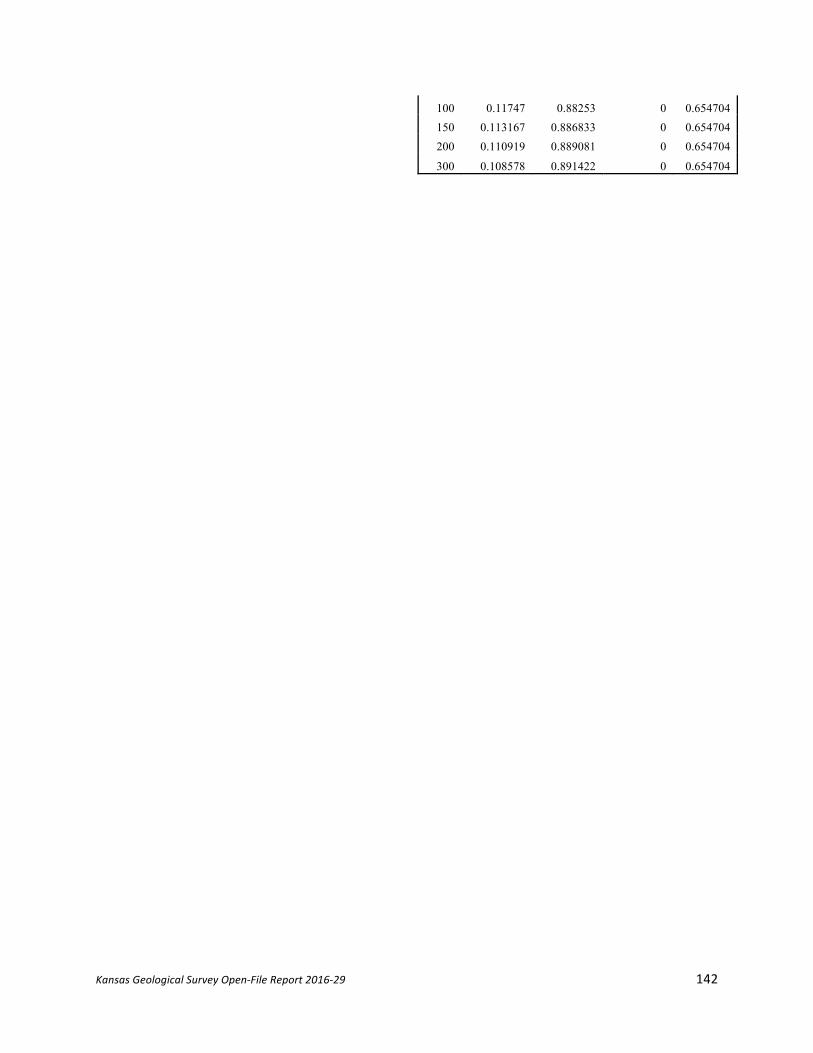
Kansas Geological Survey Open-File Report 2016-29 142
100 0.11747 0.88253 0 0.654704
150 0.113167 0.886833 0 0.654704
200 0.110919 0.889081 0 0.654704
300 0.108578 0.891422 0 0.654704
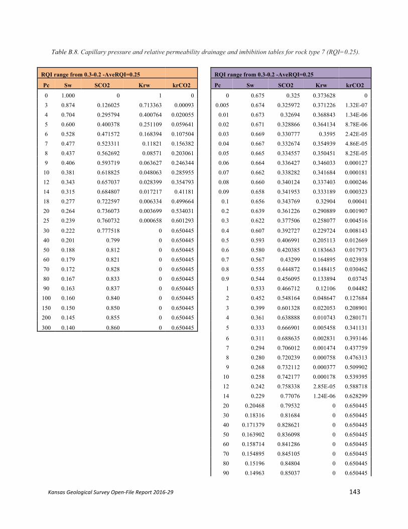
Kansas Geological Survey Open-File Report 2016-29 143
Table B.8. Capillary pressure and relative permeability drainage and imbibition tables for rock type 7 (RQI=0.25).
RQI range from 0.3-0.2 -AveRQI=0.25
RQI range from 0.3-0.2 -AveRQI=0.25
Pc Sw SCO2 Krw krCO2
Pc Sw SCO2 Krw krCO2
0 1.000 0 1 0
0 0.675 0.325 0.373628 0 3 0.874 0.126025 0.713363 0.00093
0.005 0.674 0.325972 0.371226 1.32E-07
4 0.704 0.295794 0.400764 0.020055
0.01 0.673 0.32694 0.368843 1.34E-06 5 0.600 0.400378 0.251109 0.059641
0.02 0.671 0.328866 0.364134 8.78E-06
6 0.528 0.471572 0.168394 0.107504
0.03 0.669 0.330777 0.3595 2.42E-05 7 0.477 0.523311 0.11821 0.156382
0.04 0.667 0.332674 0.354939 4.86E-05
8 0.437 0.562692 0.08571 0.203061
0.05 0.665 0.334557 0.350451 8.25E-05 9 0.406 0.593719 0.063627 0.246344
0.06 0.664 0.336427 0.346033 0.000127
10 0.381 0.618825 0.048063 0.285955
0.07 0.662 0.338282 0.341684 0.000181 12 0.343 0.657037 0.028399 0.354793
0.08 0.660 0.340124 0.337403 0.000246
14 0.315 0.684807 0.017217 0.41181
0.09 0.658 0.341953 0.333189 0.000323 18 0.277 0.722597 0.006334 0.499664
0.1 0.656 0.343769 0.32904 0.00041
20 0.264 0.736073 0.003699 0.534031
0.2 0.639 0.361226 0.290889 0.001907 25 0.239 0.760732 0.000658 0.601293
0.3 0.622 0.377506 0.258077 0.004516
30 0.222 0.777518 0 0.650445
0.4 0.607 0.392727 0.229724 0.008143 40 0.201 0.799 0 0.650445
0.5 0.593 0.406991 0.205113 0.012669
50 0.188 0.812 0 0.650445
0.6 0.580 0.420385 0.183663 0.017973 60 0.179 0.821 0 0.650445
0.7 0.567 0.43299 0.164895 0.023938
70 0.172 0.828 0 0.650445
0.8 0.555 0.444872 0.148415 0.030462 80 0.167 0.833 0 0.650445
0.9 0.544 0.456095 0.133894 0.03745
90 0.163 0.837 0 0.650445
1 0.533 0.466712 0.12106 0.04482 100 0.160 0.840 0 0.650445
2 0.452 0.548164 0.048647 0.127684
150 0.150 0.850 0 0.650445
3 0.399 0.601328 0.022053 0.208901 200 0.145 0.855 0 0.650445
4 0.361 0.638888 0.010743 0.280171
300 0.140 0.860 0 0.650445
5 0.333 0.666901 0.005458 0.341131
6 0.311 0.688635 0.002831 0.393146
7 0.294 0.706012 0.001474 0.437759
8 0.280 0.720239 0.000758 0.476313
9 0.268 0.732112 0.000377 0.509902
10 0.258 0.742177 0.000178 0.539395
12 0.242 0.758338 2.85E-05 0.588718
14 0.229 0.77076 1.24E-06 0.628299
20 0.20468 0.79532 0 0.650445
30 0.18316 0.81684 0 0.650445
40 0.171379 0.828621 0 0.650445
50 0.163902 0.836098 0 0.650445
60 0.158714 0.841286 0 0.650445
70 0.154895 0.845105 0 0.650445
80 0.15196 0.84804 0 0.650445
90 0.14963 0.85037 0 0.650445
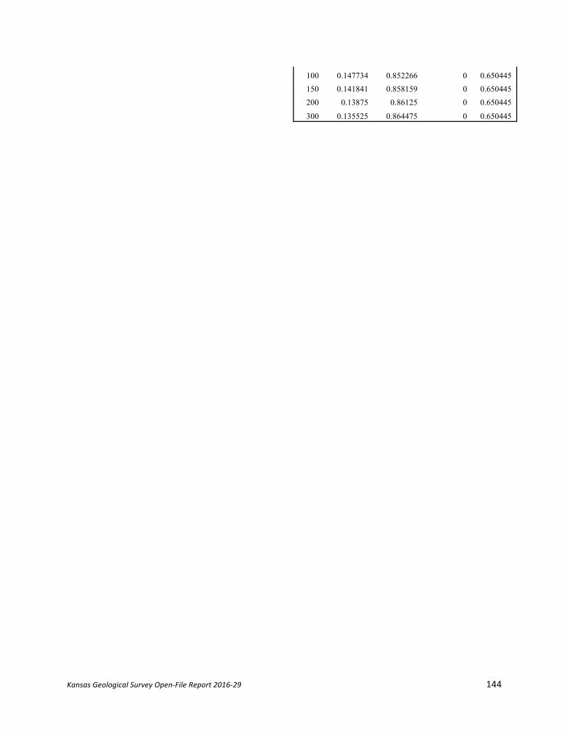
Kansas Geological Survey Open-File Report 2016-29 144
100 0.147734 0.852266 0 0.650445
150 0.141841 0.858159 0 0.650445
200 0.13875 0.86125 0 0.650445
300 0.135525 0.864475 0 0.650445

Kansas Geological Survey Open-File Report 2016-29 145
Table B.9. Capillary pressure and relative permeability drainage and imbibition tables for rock type 8 (RQI=0.15).
RQI range from 0.1-0.01 -AveRQI=0.15
RQI range from 0.1-0.01 -AveRQI=0.15
Pc Sw SCO2 Krw krCO2
Pc Sw SCO2 Krw krCO2
0 1.000 0 1 0
0 0.698 0.3025 0.445231 0 5 0.941 0.059018 0.838383 0.000148
0.005 0.696 0.303506 0.441579 1.36E-06
6 0.826 0.174245 0.56222 0.006198
0.01 0.696 0.304011 0.439754 3.44E-06 7 0.742 0.257984 0.394669 0.024002
0.02 0.695 0.305017 0.43613 1.08E-05
8 0.678 0.321723 0.286162 0.051411
0.03 0.694 0.30602 0.43254 2.28E-05 9 0.628 0.37194 0.212433 0.084796
0.04 0.693 0.307018 0.428985 3.98E-05
10 0.587 0.412576 0.160468 0.121264
0.05 0.692 0.308013 0.425464 6.18E-05 12 0.526 0.474422 0.094815 0.196341
0.06 0.691 0.309003 0.421976 8.91E-05
14 0.481 0.519367 0.057484 0.268306
0.07 0.690 0.309989 0.418521 0.000122 18 0.419 0.580531 0.021146 0.393949
0.08 0.689 0.310971 0.4151 0.00016
20 0.398 0.602342 0.012351 0.447404
0.09 0.688 0.31195 0.41171 0.000204 25 0.358 0.642253 0.002198 0.55825
0.1 0.687 0.312924 0.408353 0.000253
30 0.331 0.669422 0 0.64403
0.2 0.678 0.322455 0.376468 0.00106 40 0.296 0.704 0 0.64403
0.3 0.668 0.331617 0.347426 0.002437
50 0.274 0.726 0 0.64403
0.4 0.660 0.340431 0.320934 0.004363 60 0.260 0.740 0 0.64403
0.5 0.651 0.348917 0.296735 0.006805
70 0.249 0.751 0 0.64403
0.6 0.643 0.357093 0.274601 0.009727 80 0.241 0.759 0 0.64403
0.7 0.635 0.364976 0.254329 0.013089
90 0.235 0.765 0 0.64403
0.8 0.627 0.372581 0.23574 0.016856 100 0.230 0.770 0 0.64403
0.9 0.620 0.379925 0.218674 0.020989
150 0.214 0.786 0 0.64403
1 0.613 0.387019 0.202989 0.025457 200 0.206 0.794 0 0.64403
2 0.553 0.446681 0.099601 0.082468
300 0.197 0.803 0 0.64403
3 0.509 0.491341 0.0509 0.149335
4 0.474 0.526085 0.026542 0.216548
5 0.446 0.553924 0.013886 0.280345
6 0.423 0.576754 0.007172 0.339428
7 0.404 0.595832 0.003592 0.393561
8 0.388 0.612026 0.001704 0.442954
9 0.374 0.625951 0.00074 0.487988
10 0.362 0.638059 0.000278 0.529089
12 0.342 0.658102 1.31E-05 0.601124
14 0.325968 0.674032 0 0.64403
20 0.293082 0.706918 0 0.64403
30 0.262675 0.737325 0 0.64403
40 0.245378 0.754622 0 0.64403
50 0.234156 0.765844 0 0.64403
60 0.226259 0.773741 0 0.64403
70 0.220385 0.779615 0 0.64403
80 0.215838 0.784162 0 0.64403
90 0.212208 0.787792 0 0.64403

Kansas Geological Survey Open-File Report 2016-29 146
100 0.20924 0.79076 0 0.64403
150 0.19994 0.80006 0 0.64403
200 0.195016 0.804984 0 0.64403
300 0.189845 0.810155 0 0.64403
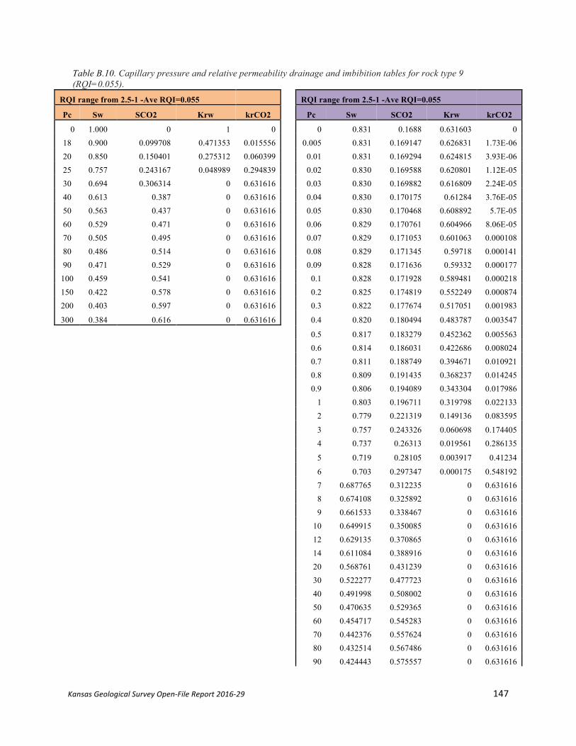
Kansas Geological Survey Open-File Report 2016-29 147
Table B.10. Capillary pressure and relative permeability drainage and imbibition tables for rock type 9 (RQI=0.055).
RQI range from 2.5-1 -Ave RQI=0.055
RQI range from 2.5-1 -Ave RQI=0.055
Pc Sw SCO2 Krw krCO2
Pc Sw SCO2 Krw krCO2
0 1.000 0 1 0
0 0.831 0.1688 0.631603 0 18 0.900 0.099708 0.471353 0.015556
0.005 0.831 0.169147 0.626831 1.73E-06
20 0.850 0.150401 0.275312 0.060399
0.01 0.831 0.169294 0.624815 3.93E-06 25 0.757 0.243167 0.048989 0.294839
0.02 0.830 0.169588 0.620801 1.12E-05
30 0.694 0.306314 0 0.631616
0.03 0.830 0.169882 0.616809 2.24E-05 40 0.613 0.387 0 0.631616
0.04 0.830 0.170175 0.61284 3.76E-05
50 0.563 0.437 0 0.631616
0.05 0.830 0.170468 0.608892 5.7E-05 60 0.529 0.471 0 0.631616
0.06 0.829 0.170761 0.604966 8.06E-05
70 0.505 0.495 0 0.631616
0.07 0.829 0.171053 0.601063 0.000108 80 0.486 0.514 0 0.631616
0.08 0.829 0.171345 0.59718 0.000141
90 0.471 0.529 0 0.631616
0.09 0.828 0.171636 0.59332 0.000177 100 0.459 0.541 0 0.631616
0.1 0.828 0.171928 0.589481 0.000218
150 0.422 0.578 0 0.631616
0.2 0.825 0.174819 0.552249 0.000874 200 0.403 0.597 0 0.631616
0.3 0.822 0.177674 0.517051 0.001983
300 0.384 0.616 0 0.631616
0.4 0.820 0.180494 0.483787 0.003547
0.5 0.817 0.183279 0.452362 0.005563
0.6 0.814 0.186031 0.422686 0.008024
0.7 0.811 0.188749 0.394671 0.010921
0.8 0.809 0.191435 0.368237 0.014245
0.9 0.806 0.194089 0.343304 0.017986
1 0.803 0.196711 0.319798 0.022133
2 0.779 0.221319 0.149136 0.083595
3 0.757 0.243326 0.060698 0.174405
4 0.737 0.26313 0.019561 0.286135
5 0.719 0.28105 0.003917 0.41234
6 0.703 0.297347 0.000175 0.548192
7 0.687765 0.312235 0 0.631616
8 0.674108 0.325892 0 0.631616
9 0.661533 0.338467 0 0.631616
10 0.649915 0.350085 0 0.631616
12 0.629135 0.370865 0 0.631616
14 0.611084 0.388916 0 0.631616
20 0.568761 0.431239 0 0.631616
30 0.522277 0.477723 0 0.631616
40 0.491998 0.508002 0 0.631616
50 0.470635 0.529365 0 0.631616
60 0.454717 0.545283 0 0.631616
70 0.442376 0.557624 0 0.631616
80 0.432514 0.567486 0 0.631616
90 0.424443 0.575557 0 0.631616

Kansas Geological Survey Open-File Report 2016-29 148
100 0.41771 0.58229 0 0.631616
150 0.395809 0.604191 0 0.631616
200 0.383707 0.616293 0 0.631616
300 0.370611 0.629389 0 0.631616
Kansas Geological Survey Open-File Report 2016-29 149
References
Bennion, B., and Bachu, S., 2007, Relative permeability characteristics for supercritical CO2 displacing water in a variety of potential sequestration zones: Society of Petroleum Engineers, SPE-95547-MS.
Bennion, B., and Bachu, S., 2010, Drainage and imbibition CO2/brine relative permeability
curves at reservoir conditions for high-permeability carbonate rocks: Society of Petroleum Engineers, SPE 134028-MS.
Benson, S., 2005, Overview of geologic storage of CO2, in carbon dioxide capture for storage in
deep geologic formations, Volume 2—Results from the CO2 capture project: Elsevier Publishing, UK.
Burnside, N. M., and Naylor, M., 2014, Review and implications of relative permeability of
CO2/brine systems and residual trapping of CO2: Int. J. Greenh. Gas Control, 23, p. 1–11 Bui, L. H., Tsau, J. S., and Willhite, G. P., 2010, Laboratory investigations of CO2 near-miscible
application in Arbuckle Reservoir: SPE Improved Oil Recovery Symposium, Tulsa, Oklahoma, 24–28 April 2010, SPE Publication 129710.
Carter, R. D., and Tracy, G. W., 1960, An improved method for calculating water influx:
Petroleum Transactions, AIME, v. 219, p. 415–417. Chang, K. W., Minkoff, S. E., and Bryant, S. L., 2009, Simplified model for CO2 leakage and its
attenuation due to geological structures: Energy Procedia, v. 1, p. 3,453–3460. Dake, L. P., 1978, Fundamentals of Reservoir Engineering, Chapter 9, Elsevier Scientific
Publishing Co., 1978. Deutsch, C.V. 2002. Geostatistical reservoir modeling. Oxford University Press, Inc., New York,
New York. FutureGen Industrial Alliance, 2013, Underground injection control permit applications for
FutureGen 2.0 Morgan County Class VI UIC Wells 1, 2, 3, and 4, Jacksonville, Illinois. Kestin, J., Khalifa, H. E., and Correia, R. J., 1981, Tables of the dynamic and kinematic viscosity
of aqueous NaCl solutions in the temperature range 20–150 °C and the pressure range 0.1–35 MPa: Journal of Physical and Chemical Reference Data, NIST, v. 10, p. 71–88.
Krevor, P., and Benson, S. M., 2012, Capillary pressure and heterogeneity for the CO2/water
system in sandstone rocks at reservoir conditions: Advances in Water Resources, v. 38, p. 48–59, ISSN: 0309-1708
Krevor, P., and Benson, S. M., 2015, Accurate determination of characteristic relative
permeability curves: Advances in Water Resources, v. 83, p. 376–388

Kansas Geological Survey Open-File Report 2016-29 150
Li, Y. K., and Nghiem, L. X., 1986, Phase equilibrium of oil, gas and water/brine mixtures from
a cubic equation of state and Henry’s Law: Canadian Journal of Chemical Engineering, June, p. 486–496.
Loucks, R. G., 1999, Paleocave carbonate reservoirs: Origins, burial-depth modifications, spatial
complexity, and reservoir implications: The American Association of Petroleum Geologists, Bulletin, v. 83, no. 11.
Lucia, F. J., 1999, Carbonate reservoir characterization: New York, Springer-Verlag, 226 p. Pau, G. S. H., Bell, J. B., Pruess, K., Almgren, A. S., Lijewski, M. J., and Zhang, K., 2010, High
resolution simulation and characterization of density-driven flow in CO2 storage in saline aquifers: Advances in Water Resources, v. 33, no. 4, p. 443–455.
Søreide, I., and Whitson, C. H., 1992, Peng-Robinson predictions for hydrocarbons, CO2, N2,
and H2S with pure water and NaCI brine: Fluid Phase Equilibria, v. 77, p. 217–240.