AVO and Inversion - Part 2

A summary of AVO and Inversion Techniques

Dr. Brian Russell

Introduction

The Amplitude Variations with Offset (AVO) technique has

grown to include a multitude of sub-techniques, each with its

own assumptions.

AVO techniques can be subdivided as either:

(1) seismic reflectivity or (2) impedance methods.

Seismic reflectivity methods include: Near and Far stacks,

Intercept vs Gradient analysis and the fluid factor.

Impedance methods include: P and S-impedance inversion,

Lambda-mu-rho, Elastic Impedance and Poisson

Impedance.

The objective of this section is to make sense of all of these

methods and show how they are related.

Let us start by looking at the different ways in which a

geologist and geophysicist look at data.

From Geology to Geophysics

For a layered earth, a well log measures a parameter P for each

layer and the seismic trace measures the interface reflectivity R.

Pi

Pi+1

Ri

Well Log Reflectivity

Layer i

Layer i+1

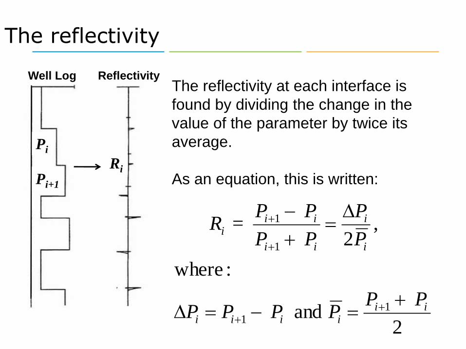
The reflectivity at each interface is

found by dividing the change in the

value of the parameter by twice its

average.

The reflectivity

Pi

Pi+1

Ri

Well Log Reflectivity

2and

:where

,2

11

1

1

iiiiii

i

i

ii

iii

PPP PPP

P

P

PP

PP = R

As an equation, this is written:

One extra thing to observe is that the seismic trace is the

convolution of the reflectivity with a wavelet (S = W*R).

The convolutional model

Parameter Reflectivity

Wavelet

Seismic

Which parameter?

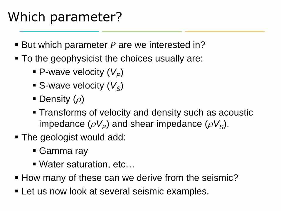
But which parameter P are we interested in?

To the geophysicist the choices usually are:

P-wave velocity (VP)

S-wave velocity (VS)

Density (r)

Transforms of velocity and density such as acoustic

impedance (rVP) and shear impedance (rVS).

The geologist would add:

Gamma ray

Water saturation, etc…

How many of these can we derive from the seismic?

Let us now look at several seismic examples.

The zero-angle trace

can be modeled

using a well known

model, where the

trace is the

convolution of the

acoustic impedance

reflectivity with the

wavelet.

Note: the stack is

only approximately

zero-angle.

The zero-angle model

Acoustic

ImpedanceReflectivity

Wavelet

W

Seismic

AI

AI = RAI

2 PVAI r

AIRWS *

Convolution

Convolution with the seismic wavelet, which can be written mathematically

as S = W*R, is illustrated pictorially below:

+ + + + =>

S = Seismic

Trace

R = Reflection

Coefficients

=*

W = Wavelet

8

A Seismic Example

The seismic

line is the

“stack” of a

series of CMP

gathers, as

shown here.

Here is a portion of a 2D

seismic line showing a

gas sand “bright-spot”.

The gas sand is

a typical Class 3

AVO anomaly.

The pre-stack gathers

• The traces in a seismic gather reflect from the subsurface at increasing

angles of incidence q, related to offset X.

• If the angle is greater than zero, notice that there is both a shear

component and a compressional component.

q1q2q3

Surface

Reflectorr1 VP1 VS1

r2 VP2 VS2

X1

X2

X3

Compression

Shear

q

Reflected

P-wave = RP(q1)

Reflected

SV-wave = RS(q1)

Transmitted

P-wave = TP(q1)

Incident

P-wave

Transmitted

SV-wave = TS(q1)

VP1 , VS1 , r1

VP2 , VS2 , r2

q1

1

q1

q2

2

More technically speaking, if q > 0°, an incident P-wave will produce

both P and SV reflected and transmitted waves. This is called mode

conversion.

Mode Conversion of an incident P-Wave

11

12

The Zoeppritz Equations (1919)

1

1

1

1

1

2

11

222

11

221

1

11

22

11

1222

2

2

11

1

2

221

1

11

2211

2211

1

1

1

1

2cos

2sin

cos

sin

2sin2cos2sin2cos

2cos2sin2cos2sin

sincossincos

cossincossin

)(

)(

)(

)(

q

q

q

r

r

r

r

r

rq

r

rq

qq

qq

q

q

q

q

P

S

P

P

P

S

S

PS

PS

PS

S

P

S

P

S

P

V

V

V

V

V

V

V

VV

VV

VV

V

V

T

T

R

R

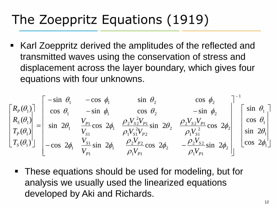
Karl Zoeppritz derived the amplitudes of the reflected and

transmitted waves using the conservation of stress and

displacement across the layer boundary, which gives four

equations with four unknowns.

These equations should be used for modeling, but for

analysis we usually used the linearized equations

developed by Aki and Richards.

The Aki-Richards equation

The Aki-Richards equation is a linearized form of the

Zoeppritz equations which is written:

,)( DVSVP cRbRaRR q

The Aki-Richards equation says that the reflectivity at angle

q is the weighted sum of the VP, VS and density reflectivities.

,2

,2

,2

:wherer

r

D

S

SVS

P

PVP R

V

VR

V

VR

.and ,sin41,sin8,tan1

2

222

P

S

V

VKKcKba qqq

14

To understand the Aki-Richards equation, let us look at a picked

event at a given time on the 3 trace angle gather shown below:

Each pick at time t and angle q is equal to

the Aki-Richards reflectivity at that point

(after convolution with an angle-dependent

wavelet) given by the sum of the three

weighted reflectivities. If we assume that at

time t, (VS/VP)2= 0.25, we see that:

Understanding Aki-Richards

333.030tanand 25.030sin:Note

2750.0

2500.0

2333.1)30(

00tan0sin:Note2

02

)0(

22

oo

S

S

P

Po

P

oo

P

Po

P

V

V

V

VR

V

VR

r

r

r

r

t

Constant Angle

600 ms

700 ms

Picks

15o

0o

30o

15

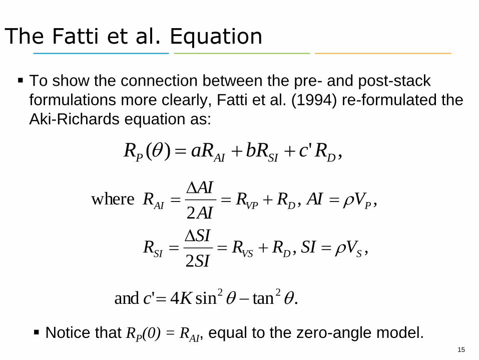
The Fatti et al. Equation

To show the connection between the pre- and post-stack

formulations more clearly, Fatti et al. (1994) re-formulated the

Aki-Richards equation as:

,')( DSIAIP RcbRaRR q

Notice that RP(0) = RAI, equal to the zero-angle model.

,,2

where PDVPAI VAIRRAI

AIR r

,,2

SDVSSI VSIRRSI

SIR r

.tansin4' and 22 qq Kc

Smith and Gidlow

Fatti et al. (1994) is a refinement of the original work of

Smith and Gidlow (1987).

The key difference between the two papers is the Smith and

Gidlow use the original Aki-Richards equation and absorb

density into VP using Gardner’s equation.

Both papers also define the Poisson’s Ratio reflectivity Rs

and the fluid factor F (which was derived from Castagna’s

mudrock line) as:

)/(16.1 where,

and ,2

PSSIAI

SIAI

VVggRRF

RRR

s

ss

17

Modified from Castagna et al, (1985)

The Mudrock Line

In non-mathematical

terms, Fatti and

Smith define F as

the difference away

from the VP versus VS

line that defines wet

sands and shales.

These differences

should indicate fluid

anomalies.

FV

P(k

m/s

ec

)

VS (km/sec)

The Intercept/Gradient method

The most common approach to AVO is the Intercept/Gradient

method, which involves re-arranging the Aki-Richards

equation to:

: where,tansinsin)( 222 qqqq VPAIP RGRR

This is again a weighted reflectivity equation with weights

of a = 1, b = sin2q, c = sin2q tan2q.

The three reflectivities are usually called A, B, and C (or:

intercept, gradient and curvature) but this obscures the

fact that only G is a new reflectivity compared with the

previous methods.

gradient. the48 DVSVP KRKRRG

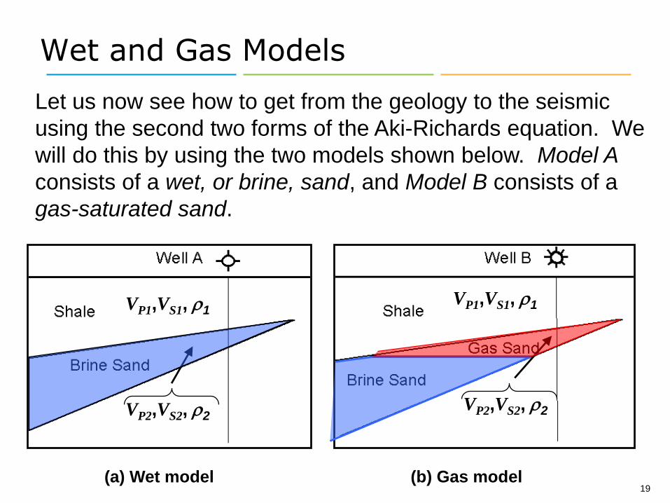
Let us now see how to get from the geology to the seismic

using the second two forms of the Aki-Richards equation. We

will do this by using the two models shown below. Model A

consists of a wet, or brine, sand, and Model B consists of a

gas-saturated sand.

Wet and Gas Models

(a) Wet model (b) Gas model

VP1,VS1, r1

VP2,VS2, r2

VP1,VS1, r1

VP2,VS2, r2

19

In the section on rock physics, we computed values for wet and

gas sands using the Biot-Gassmann equations. Recall that the

computed values were:

Wet: VP2 = 2500 m/s, VS2= 1250 m/s, r2 = 2.11 g/cc, s2 = 0.33

Gas: VP2 = 2000 m/s, VS2 = 1310 m/s, r2 = 1.95 g/cc, s2 = 0.12

Values for a typical shale are:

Shale: VP1 = 2250 m/s, VS1 = 1125 m/s, r1 = 2.0 g/cc, s1 = 0.33

The next four figures will show the results of modeling with the

Intercept/Gradient and Fatti equations.

Model Values

20

This figure on the right

shows the AVO curves

computed using the

Zoeppritz equations

and the two and three

term ABC equation, for

the gas sand model.

Notice the strong

deviation for the two

term versus three term

sum.

Zoeppritz vs the ABC Method – Gas Sand

Zoeppritz

AB method

ABC method

21August 2014

This figure on the

right shows the AVO

curves computed

using the Zoeppritz

equations and the

two and three term

ABC equation, for

the wet sand model.

Again, notice the

strong deviation for

the two term versus

three term sum.

Zoeppritz vs the ABC Method – Wet Sand

Zoeppritz

AB method

ABC method

22August 2014

This figure on the

right shows the AVO

curves computed

using the Zoeppritz

equations and the

two and three term

Fatti equation, for

the gas sand model.

Notice there is less

deviation between

the two term and

three term sum than

with the ABC

approach.

Zoeppritz vs the Fatti Method – Gas Sand

Zoeppritz

Fatti method,

two term

Fatti method,

three term

23August 2014

Zoeppritz vs the Fatti Method – Wet Sand

Zoeppritz

Fatti method,

two term

Fatti method,

three term

24August 2014

This figure on the

right shows the AVO

curves computed

using the Zoeppritz

equations and the two

and three term Fatti

equation, for the wet

sand model.

As in the gas sand

case, there is less

deviation between the

two term and three

term sum than with

the ABC approach.

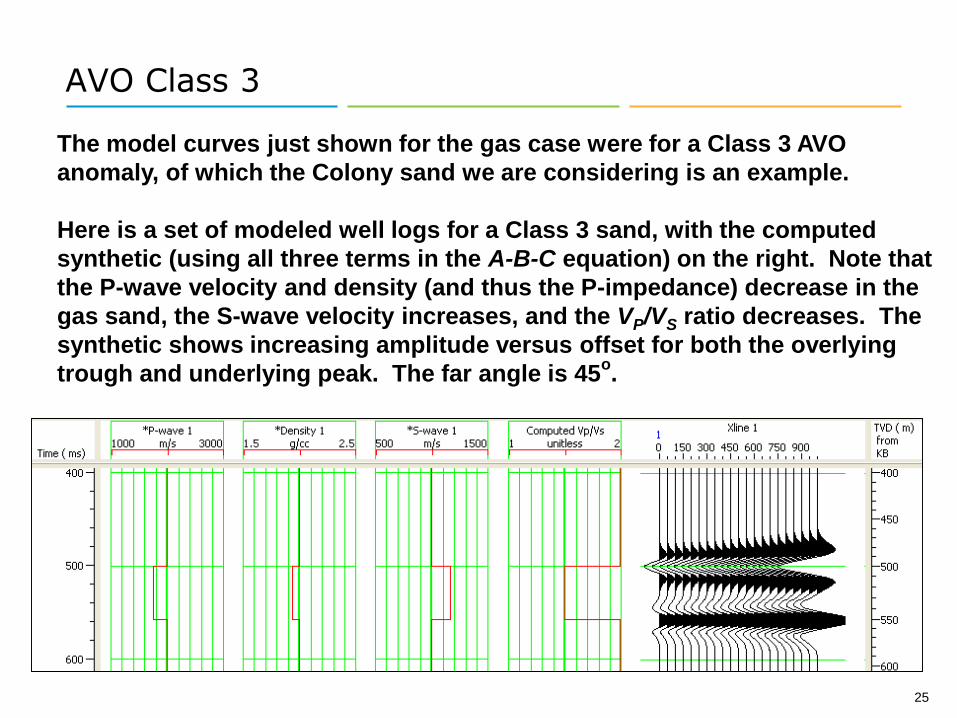
AVO Class 3

The model curves just shown for the gas case were for a Class 3 AVO

anomaly, of which the Colony sand we are considering is an example.

Here is a set of modeled well logs for a Class 3 sand, with the computed

synthetic (using all three terms in the A-B-C equation) on the right. Note that

the P-wave velocity and density (and thus the P-impedance) decrease in the

gas sand, the S-wave velocity increases, and the VP/VS ratio decreases. The

synthetic shows increasing amplitude versus offset for both the overlying

trough and underlying peak. The far angle is 45o.

25

AVO Class 2

There are several other AVO classes, of which Class 1 and 2 are the most

often seen.

Here is a Class 2 example well log, where the P-impedance change is very

small and the amplitude change on the synthetic is very large. Note that the

VP/VS ratio is still decreasing to 1.5, as expected in a clean gas sand (recall

the discussion in the rock physics section).

26

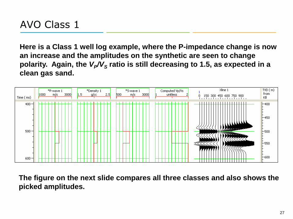
AVO Class 1

27

Here is a Class 1 well log example, where the P-impedance change is now

an increase and the amplitudes on the synthetic are seen to change

polarity. Again, the VP/VS ratio is still decreasing to 1.5, as expected in a

clean gas sand.

The figure on the next slide compares all three classes and also shows the

picked amplitudes.

The three AVO Classes

28

A comparison of the

synthetic seismic

gathers from the three

classes, where the top

and base of the gas

sand have been picked.

The picks are shown at

the bottom of the

display and clearly

show the AVO effects.

These synthetics were

created at the same

time, but in practice

class 1 sands are deep,

class 2 sands are at

medium depths and

class 3 sands are at

shallow depths.

Class 1 Class 2 Class 3

tim

e (

ms)

am

plit

ud

e

We are usually interested in modeling a lot more than one

or two layers.

Multi-layer modeling consists first of creating a stack of N

layers, generally using well logs, and defining the

thickness, P-wave velocity, S-wave velocity, and density

for each layer, as shown below:

Multi-Layer AVO Modeling

29

You must then decide what effects are to be included in the model:

primaries only, converted waves, multiples, or some combination of these.

The full solution is with a technique called Wave Equation modeling.

Multi-Layer AVO Modeling

30

AVO Modeling in our gas sand

Based on AVO theory and the rock physics of the reservoir, we can perform

AVO modeling of our earlier example, as shown above. Note that the model

result is a fairly good match to the offset stack.

P-wave Density S-wavePoisson’s

ratioSynthetic Offset Stack

31

The angle gather

Using the P-wave velocity, we can

transform the offset gathers shown

earlier to angle gathers. There are

two ways in which AVO methods

extract reflectivity from angle gathers.

q1

time

angle

Or we can extract the reflectivity

function at a single angle q.

We can perform a least-squares fit to

the reflectivity at a given time for all

angles.

qN

33

Angle

Time

(ms)

600

650

t

1 NTo estimate the reflectivities

in the Fatti method, the

amplitudes at each time t in

an N-trace angle gather are

picked as shown here.

We can solve for the

reflectivities at each time

sample using least-squares:

Estimating RAI and RSI

)(

)( 11

NP

P

D

SI

AI

R

R

matrix

weight

R

R

R

q

q

Reflectivities

Generalized inverse of

weight matrix

Observations

Smith and Gidlow’s results

Here are the

Rs and F

sections from

an offshore

field in South

Africa. Note

that the fluid

factor F

shows the fluid

anomaly the

best.

Rs section F section

Smith and Gidlow

(1987)

Fatti et al. (1994)

A comparison of a seismic amplitude map and a fluid factor

map for a gas sand play. Note the correlation of high F

values with the gas wells.

Fatti et al.’s results

F MapSeismic Amplitude Map

36

Offset+RAI

+G

- G

sin2q

Time

Regression curves are

calculated to give RAI and G

values for each time sample.

For the intercept/gradient

method, we can visualize the fit

like this:

-RAI

The Intercept/Gradient method

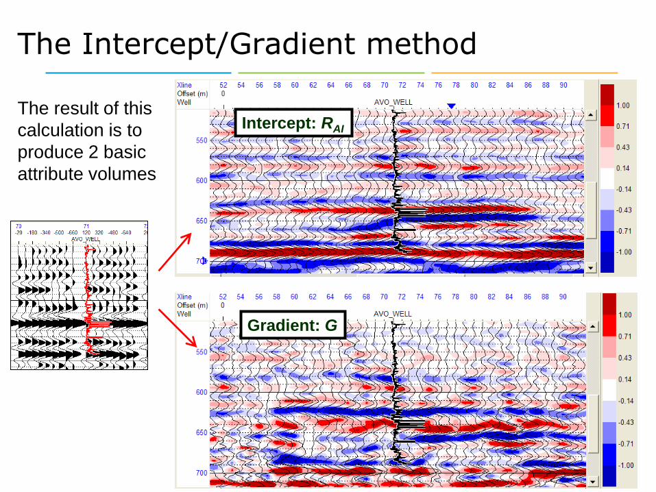
37

The result of this

calculation is to

produce 2 basic

attribute volumes

Intercept: RAI

Gradient: G

The Intercept/Gradient method

38

Intercept/Gradient combinations

The AVO product shows a positive response at the top and base of the reservoir:

Top

Base

Top

Base

The AVO difference shows pseudo-shear reflectivity:

Top

Base

The AVO sum shows pseudo-Poisson’s ratio:

39

Intercept / Gradient Cross-Plots

Here is the cross-plot of Gradient

and Intercept zones, where:

- Red = Top of Gas

- Yellow = Base of Gas

- Blue = Hard streak

- Ellipse = Mudrock trend

Below, the zones are plotted back

on the seismic section.

40

Impedance Methods

The second group of AVO methods, impedance methods,

are based on the inversion of the reflectivity estimates to

give impedance.

The simplest set of methods use the reflectivity estimates

from the Fatti et al. equation to invert for acoustic and

shear impedance, and possibly density. That is:

(Density)

Impedance)(Shear

Impedance) (Acoustic

r

r

r

D

SSI

PAI

R

VSIR

VAIR

The inversion can be done independently (separately for

each term) or using simultaneous inversion.

41

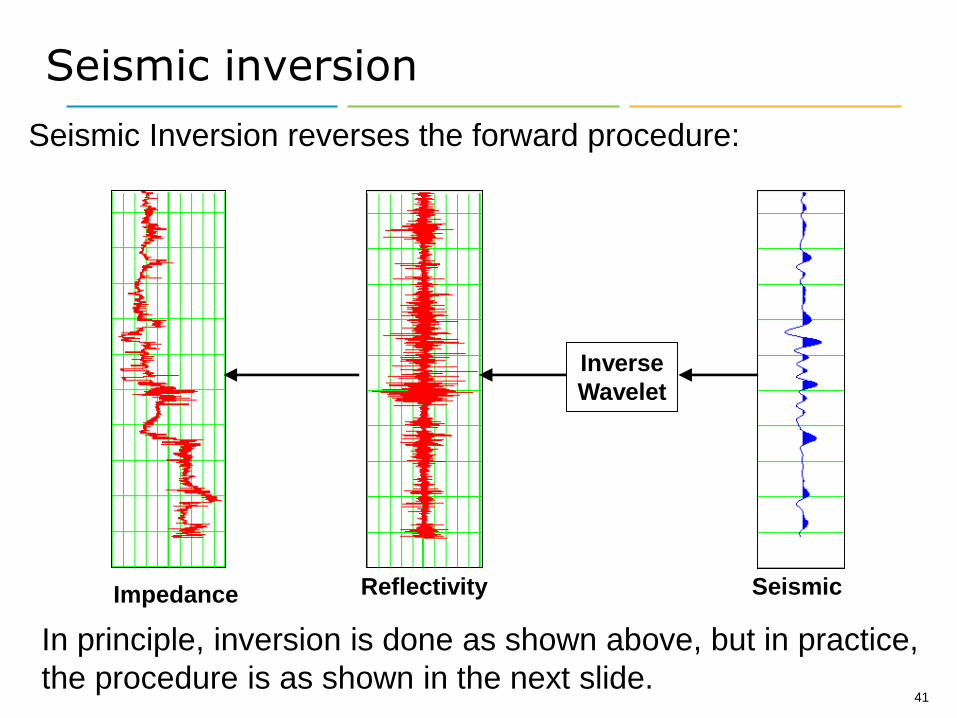
Impedance Reflectivity

Inverse

Wavelet

Seismic

Seismic Inversion reverses the forward procedure:

Seismic inversion

In principle, inversion is done as shown above, but in practice,

the procedure is as shown in the next slide.

Model-based inversion

(1) Optimally process the seismic data (2) Build model from picks and impedances

(3) Iteratively update

model until output

synthetic matches

original seismic data.

S=W*RAI M=AI=rVP

AI=rVP

In acoustic impedance

inversion the seismic,

model and output are

as shown here.

S=W*RSI M=SI=rVS

SI=rVS

In shear impedance

inversion the seismic,

model and output are

as shown here.

43

P-wave and S-wave Inversions

Here is the P-wave

inversion result.

The low acoustic

impedance below

Horizon 2

represents the gas

sand.

AI = rVP

SI = rVSHere is the S-wave

inversion result.

The gas sand is

now an increase,

since S-waves

respond to the

matrix.

44

AI/SI = rVP/rVS = VP/VS

Vp/Vs Ratio

Here is the ratio of P to S impedance, which is equal to the

ratio of P to S velocity. Notice the low ratio at the gas sand.

45

Cross-plot

When we crossplot

VP/VS ratio against P-

impedance, the zone of

low values of each

parameter should

correspond to gas, as

shown.

This zone should

correspond to gas:

46

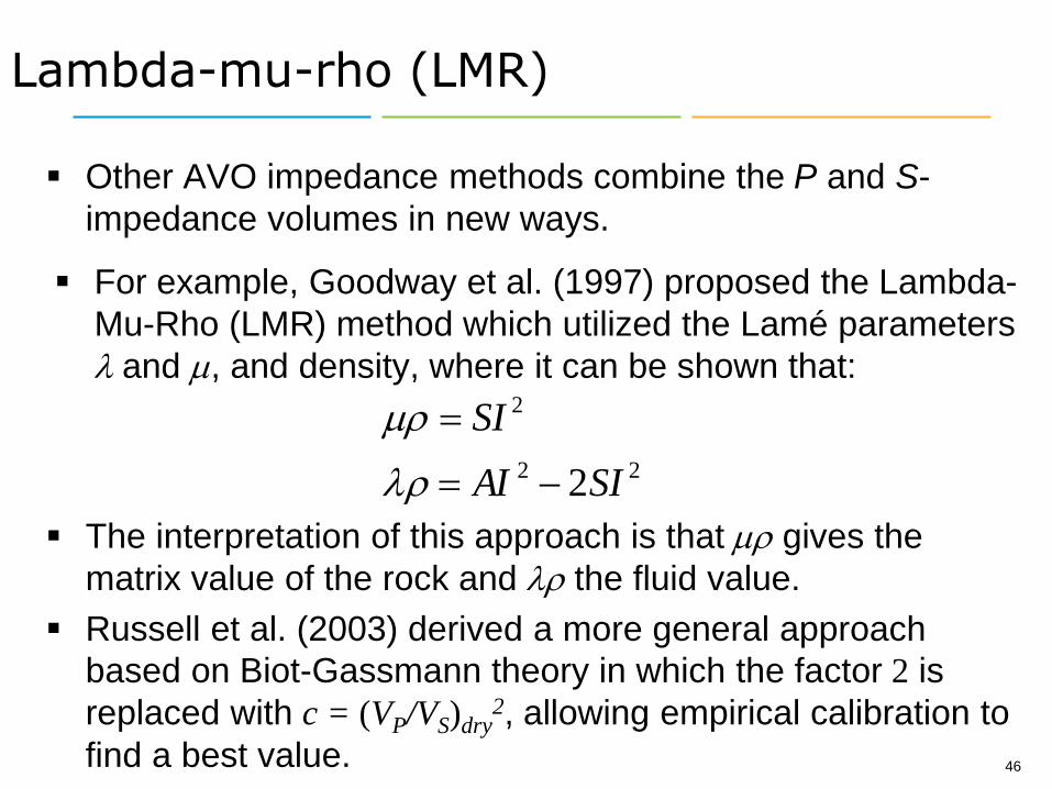
Other AVO impedance methods combine the P and S-

impedance volumes in new ways.

22

2

2SIAI

SI

r

r

Lambda-mu-rho (LMR)

The interpretation of this approach is that r gives the

matrix value of the rock and r the fluid value.

Russell et al. (2003) derived a more general approach

based on Biot-Gassmann theory in which the factor 2 is

replaced with c = (VP/VS)dry2, allowing empirical calibration to

find a best value.

For example, Goodway et al. (1997) proposed the Lambda-

Mu-Rho (LMR) method which utilized the Lamé parameters

and , and density, where it can be shown that:

47

The r and rsections derived from the AI and SI inverted sections shown earlier.

Note the decrease in r and the increase in r at the gas sand zone.

r and r example

r (lambda-rho)

r (mu-rho)

48

A cross-plot of the r and r sections, with the corresponding seismic section. Two zones are shown, where red = gas (low r values) and blue = non-gas.

Colony Sand – cross-plot

r (lambda-rho)

r

(mu

-rh

o)

Last updated: June 2008 49

One AVO reflectivity

method we did not

discuss was near

and far angle stacks,

as shown here.

Note the amplitude

of the “bright-spot”

event is stronger on

the far-angle stack

than it is on the

near-angle stack.

But what does this

mean?

Near and far trace stacks

Near angle (0-15o) stack

Far angle (15-30o) stack

50

Elastic Impedance

The equivalent impedance method to near and far angle

stacking is Elastic Impedance, or EI (Connolly,1999).

To understand EI, recall the Aki-Richards equation:

.sin21 and ,sin8,tan1

: where,222

)(

222 qqq

r

rq

KcKba

cV

Vb

V

VaR

S

S

P

PP

cb

S

a

PEI VVEIEIEI

EIR rqq

q

qq

)( where,)(ln

2

1

)(

)(

2

1)(

Connolly postulated that associated with this equation is

an underlying elastic impedance, written (where I have re-

named the reflectivity to match the EI concept):

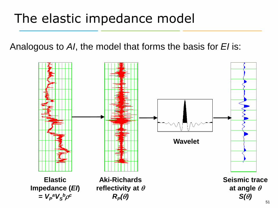
51

Elastic

Impedance (EI)

= VPaVS

brc

Aki-Richards

reflectivity at q

RP(q)

Wavelet

Seismic trace

at angle q

S(q)

Analogous to AI, the model that forms the basis for EI is:

The elastic impedance model

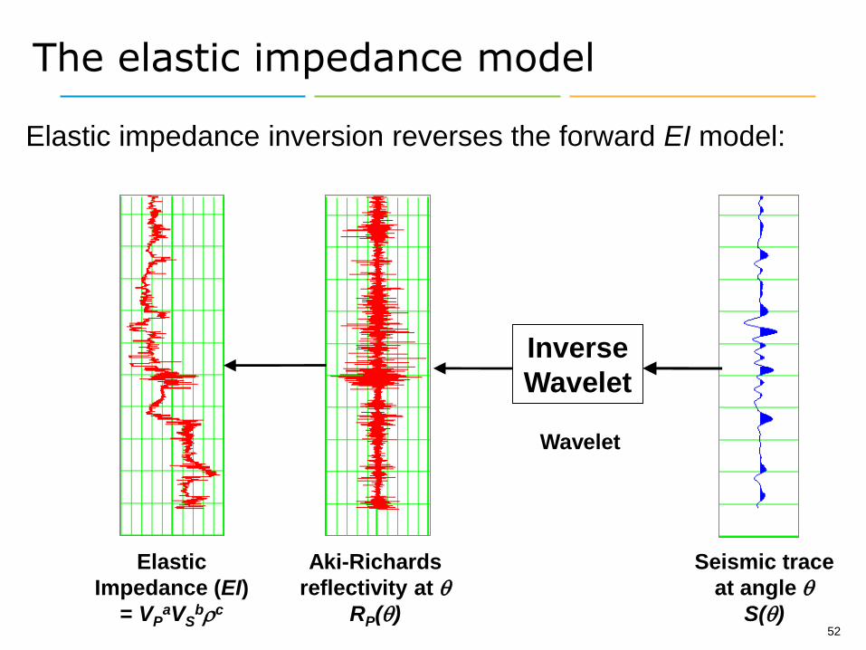
52

Elastic

Impedance (EI)

= VPaVS

brc

Aki-Richards

reflectivity at q

RP(q)

Wavelet

Seismic trace

at angle q

S(q)

The elastic impedance model

Inverse

Wavelet

Elastic impedance inversion reverses the forward EI model:

Elastic impedance inversion

(1) Optimally process the seismic data (2) Build model from picks and impedances

(3) Iteratively update

model until output

synthetic matches

original seismic data.

In elastic impedance

inversion the seismic,

model and output are

as shown here.

SEI(q)=W(q)*REI(q)cb

S

a

PVVEIM rq )(

cb

S

a

PVVEI rq )(

54

Here is the

comparison

between the EI

inversions of the

near-angle stack

and far-angle

stack.

Notice the

decrease in the

elastic impedance

value on the far-

angle stack.

Gas sand case study

EI(7.5o)

EI(22.5o)

The figures show the (a) crossplot between near and far EI logs, and (b) the

zones on the logs. Notice the clear indication of the gas sand (yellow).

EI from logs

(a) (b)

EI_Near EI_Far

56

Gas sand case study

This figure shows a crossplot

between EI at 7.5o and EI at 22.5o.

The background trend is the grey

ellipse, and the anomaly is the yellow

ellipse. As shown below, the yellow

zone corresponds to the known gas

sand.

EI at 7.5o

EI at 22.5

o

57

Since EI values do not scale correctly for different angles,

Whitcombe et al. (2002) created a new method (EEI) that

did scale correctly, and was extended to predict other rock

physics and fluid parameters (using the c factor).

Extended Elastic Impedance (EEI)

I will not go into

the details today,

but here is an

example of

predicting Vp/Vs

ratio using our

previous example,

where the units are

Elastic Impedance.

58

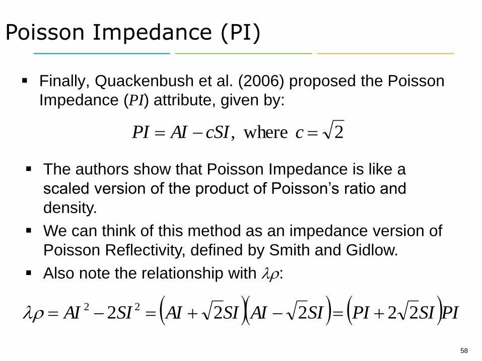
Finally, Quackenbush et al. (2006) proposed the Poisson

Impedance (PI) attribute, given by:

2 where, ccSIAIPI

Poisson Impedance (PI)

The authors show that Poisson Impedance is like a

scaled version of the product of Poisson’s ratio and

density.

We can think of this method as an impedance version of

Poisson Reflectivity, defined by Smith and Gidlow.

Also note the relationship with r:

PISIPISIAISIAISIAI 22222 22 r

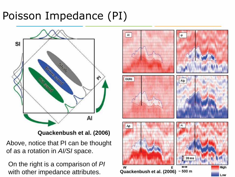
59

Above, notice that PI can be thought

of as a rotation in AI/SI space.

Poisson Impedance (PI)

On the right is a comparison of PI

with other impedance attributes.

Quackenbush et al. (2006)

Quackenbush et al. (2006)

VP(0o)

VP(45o)

VP(90o)

We will consider the cases of Transverse Isotropy with a

vertical symmetry axis, or VTI, and Transverse Isotropy

with a Horizontal symmetry axis, or HTI.

Let us finish with a discussion of anisotropic effects.

In an isotropic earth P and S-wave velocities are

independent of angle.

In an anisotropic earth, velocities and other parameters

are dependent on direction, as shown below.

Anisotropic effects

60

VTI – AVO Effects

61

qq

q

q

22

2

tansin2

sin2

)(

C

BARVTI

The VTI model consists of horizontal

layers and can be extrinsic, caused by

fine layering of the earth, or intrinsic,

caused by particle alignment as in a

shale. It can be modeled as follows,

where and are the change in

Thomsen’s first two anisotropic

parameters across a boundary:

A VTI shale over an isotropic wet sand

can create the appearance of a gas

sandstone anomaly, as shown here:

Class 1

Class 2

Class 3

Isotropic

--- Anisotropic = -0.15

= -0.3

Adapted from Blangy (1997)

In this display, the synthetic responses for a shallow gas sand in

Alberta are shown. Note the difference due to anisotropy.

(a) Isotropic (b) Anisotropic (a) – (b)

Anisotropic AVO Synthetics

62

HTI effects on AVO

63

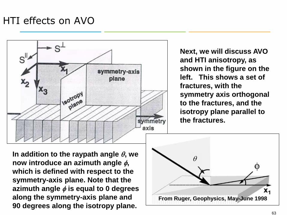
Next, we will discuss AVO

and HTI anisotropy, as

shown in the figure on the

left. This shows a set of

fractures, with the

symmetry axis orthogonal

to the fractures, and the

isotropy plane parallel to

the fractures.

In addition to the raypath angle q, we

now introduce an azimuth angle ,

which is defined with respect to the

symmetry-axis plane. Note that the

azimuth angle is equal to 0 degrees

along the symmetry-axis plane and

90 degrees along the isotropy plane.

q

From Ruger, Geophysics, May-June 1998

Modeling HTI

64

.sin2

1

,82

1

:where

tansincos

sincos

)(2)(

2

)(

222

22

VV

HTI

P

SV

HTI

HTI

HTIHTI

C

V

VB

CC

BBAR

qq

q

HTI anisotropy can be modeled with

the following equation, where is

Thomsen’s third anisotropic

parameter and (V) indicates with

respect to vertical. When = 0, along

the isotropy plane, we get the

isotropic equation, as expected:

The reflection coefficients for a

model where only changes, as

a function of incidence angle for

0, 30, 60 and 90 degrees azimuth.

Isotropy plane:

Symmetry-axis

plane:

Fracture Interpretation

Edge

Effects

Orientation

of Fault

Direction of Line is

estimated fault strike,

length of line and color

is estimated crack

density

AVO Fracture Analysis

measures fracture

volume from differences

in AVO response with

Azimuth. Fracture strike

is determined where this

difference is a maximum.

Interpreted FaultsFractures abutting

the fault

Fractures curling

into the fault

Oil Well

Courtesy: Dave Gray, CGGVeritas65

Summary of AVO methods

AVO

Methods

Seismic

Reflectivity

Impedance

Methods

Near and

Far Stack

Intercept

Gradient

Fluid

Factor

Acoustic

and Shear

Impedance

Elastic

Impedance

LMR

EEI

PI

67

Seismic reflectivity methods

The advantages of AVO methods based on seismic

reflectivity are that:

They are robust and easy to derive.

They allow the data to “speak for itself” since

their interpretation relies on detecting deviations

away from a background trend.

The disadvantage of AVO methods based on

seismic reflectivity is that:

They do not give geologists what they really

want, which is some physical parameter with a

trend.

68

Impedance methods

The advantages of AVO and inversion methods based on

impedance are that:

They give geologists what they want: a physical

parameter with a trend.

They can be transformed to reservoir properties.

The disadvantages of AVO and inversion methods based

on impedance are as follows:

The original data has to be transformed from its

natural reflectivity form.

Care must be taken to derive a good quality

inversion.

Conclusions

This presentation has been a brief overview of the various

methods used in Amplitude Variations with Offset (AVO)

and pre-stack inversion.

I showed that all of these methods are based of the Aki-

Richards approximation to the Zoeppritz equations.

I then subdivided these techniques as either:

(1) seismic reflectivity or (2) impedance methods.

Seismic reflectivity methods are straightforward to derive

and to interpret but do not give us physical parameters.

Impedance methods are more difficult to derive but give us

physical parameters including reservoir properties.

In the final analysis, there is no single “best” method for

solving all your exploration objectives. Pick the method that

works best in your area.