reservoir and mixer constrained scheduling for sample preparation …€¦ · · 2017-10-25indian...
TRANSCRIPT

INDIAN INSTITUTE OF TECHNOLOGY ROORKEE
Reservoir and Mixer Constrained Scheduling for Sample Preparation on Digital Microfluidic Biochips
In the 22nd Asia and South Pacific Design Automation Conference (ASP-DAC) 2017
January 16-19, 2017
Authored by:
Varsha Agarwal1, Ananya Singla1, Mahammad Samiuddin2, Sudip Roy1, Tsung-Yi Ho3, Indranil Sengupta2 and Bhargab B. Bhattacharya4
Presented by: Varsha Agarwal, Department of Computer Science and Engineering,
Indian Institute of Technology Roorkee, India
1CoDA Laboratory, Dept. of CSE, IIT Roorkee, India2Dept. of CSE, IIT Kharagpur, India
3Dept. of CS, National Tsing Hua University, Hsinchu, Taiwan4Advanced Computing and Microelectronics Unit, ISI Kolkata, India

Outline of the Talk
• Introduction
• Basic Preliminaries
• Prior Work
• Motivation
• Reservoir Constrained Optimal Scheduling
• Reservoir and Mixer Constrained Scheduling• Problem Formulation
• Proposed Scheme
• Simulation Results
• Conclusions and Future Work
2

Introduction
• Microfluidic biochip, also termed as lab-on-a-chip (LoC), automatesthe repetitive work in laboratory by replacing complex equipment withcompact integrated systems
Microfluidic Biochip
Digital Microfluidic Biochip (DMFB)
Continuous flow Microfluidic Biochip (CMFB)
3
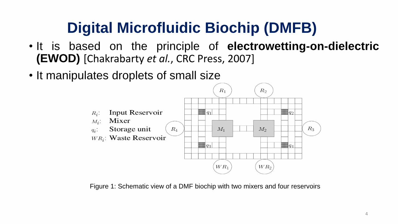
Digital Microfluidic Biochip (DMFB)• It is based on the principle of electrowetting-on-dielectric
(EWOD) [Chakrabarty et al., CRC Press, 2007]
• It manipulates droplets of small size
Figure 1: Schematic view of a DMF biochip with two mixers and four reservoirs
4

Basic Preliminaries
• Sample Preparation• Mixing of two or more fluids to get desired concentration
• Mixing tree• The step-wise processing for the generation of target concentration from
the supply of input fluids is represented by a binary mixing tree
C B
C
C
A
A
Figure 2: MinMix mixing tree for the mixture (A:B:C) = (5:4:7)
5

Basic Preliminaries (cont.)
• Reservoir Switching• At some instance of time, it is required to unload the previous reagent, wash
the reservoir and load this reservoir with new reagent. We refer this processof unloading, washing and loading as ‘switching’
• Reservoir switching takes more time than mixing [Rensch et al., Lab Chip, 2014]
Figure 3: Schematic view of the mechanical process of (a) loading, (b) unloading, (c) washing, and
(d) reloading of the reservoir at a dispenser
6

Prior Work: Mixing algorithms
• MinMix [Thies et al., Natural Computing, 2008]• Scans N d-bits of the binary fractions corresponding to the target CFs N
reagents from right to left
• RMA [Roy et al., VLSID, 2011 & Roy et al., TODAES, 2015]• Based on fractional decomposition of algebraic expression of a target
ratio
• Minimize reagent usage, droplet transportation time and storage
requirement
• CoDOS [Liu et al., ICCAD, 2013]• Generates a recipe matrix that contains the CF of each reagent fluid in
binary representation
• Find out the rectangle within the recipe matrix for possible dilution
operations that can be shared
• Droplet sharing in the mixing tree
7

Prior Work (cont.): Scheduling algorithm
• Optimal Scheduling [Luo and Akella, TASE, 2011]• It schedules the given mixing tree in the minimum total mixing
(completion) time
• Optimal scheduling algorithm work as follows:• Given a following mixing tree to be scheduled with 2 mixers and no reservoir
constrained
4
2 3
1
8

Prior Work (cont.)
At t = 1
4
2 3
1
M1
M2
4
2 3
1
M1
M2
At t = 2
M1
4
2 3
1
M1
M2
At t = 3
M1
M1
• Optimal Scheduling [Luo and Akella, TASE, 2011]
9

Motivation: Why Reservoir Switching Required?
• DMFB is small in size, so there is limited amount of resources thatcan be placed on it
• For real-life applications, while performing automated samplepreparation we need more reagents than the number of reservoirsavailable
10

Reservoir Constrained Optimal Scheduling (ROS)
• Modified optimal scheduling considering reservoir as aconstrained is called Reservoir Constrained Optimal Scheduling(ROS)
• The reservoirs are loaded or switched with the required reagentsin level wise order
11

ROS Example
• Given a following CoDOS tree with target ratio 500 : 300 : 1000 : 500 : 100 : 100 : 25 :2475 (approximated as 6 : 4 : 13 : 6 : 1 : 1 : 1 : 32 in 64-scale). Consider the DMFBarchitecture given in Fig. 1 with 2 mixers and 4 reservoirs
9
8
7
5 6
3 4
1 2
x5 x3 x7 x6
x3
x4 x1
x2
x8
p6
Level6
5
4
3
2
1
0
Schedule for NM = 2 and NR = 4
12

ROS Example (cont.)
9
8
7
5 6
3 4
1 2
x5 x3 x7 x6
x3
x4 x1
x2
x8
p6
Level6
5
4
3
2
1
0
At t = 0Probable list of nodes 1 2 4
Reservoirs
Available Mixers
M1 M2
13

ROS Example (cont.)
9
8
7
5 6
3 4
1 2
x5 x3 x7 x6
x3
x4 x1
x2
x8
p6
Level6
5
4
3
2
1
0
At t = 1Probable list of nodes 1 2 4
Reservoirs
Available Mixers
9
8
7
5 6
3 4
1 2
x5 x3 x7 x6
x3
x4 x1
x2
x8
p6
Level6
5
4
3
2
1
0
x5
x3
x7
x6
M1 M2
14

ROS Example (cont.)
9
8
7
5 6
3 4
1 2
x5 x3 x7 x6
x3
x4 x1
x2
x8
p6
Level6
5
4
3
2
1
0
After t = 1Probable list of nodes
Reservoirs
Available Mixers
9
8
7
5 6
3 4
1 2
x5 x3 x7 x6
x3
x4 x1
x2
x8
p6
Level6
5
4
3
2
1
0
x5
x3
x7
x6
9
8
7
5 6
3 4
1 2
x5 x3 x7 x6
x3
x4 x1
x2
x8
p6
Level6
5
4
3
2
1
0
3 4
x5
x3
x7
x6
M1 M2
M1 M2
15

ROS Example (cont.)
9
8
7
5 6
3 4
1 2
x5 x3 x7 x6
x3
x4 x1
x2
x8
p6
Level6
5
4
3
2
1
0
At t = 2Probable list of nodes
Reservoirs
Available Mixers
9
8
7
5 6
3 4
1 2
x5 x3 x7 x6
x3
x4 x1
x2
x8
p6
Level6
5
4
3
2
1
0
x5
x3
x7
x6
9
8
7
5 6
3 4
1 2
x5 x3 x7 x6
x3
x4 x1
x2
x8
p6
Level6
5
4
3
2
1
0
3 4
x4
x1
x7
x6
Number of switching required = 1
M1 M2
M1 M2
16
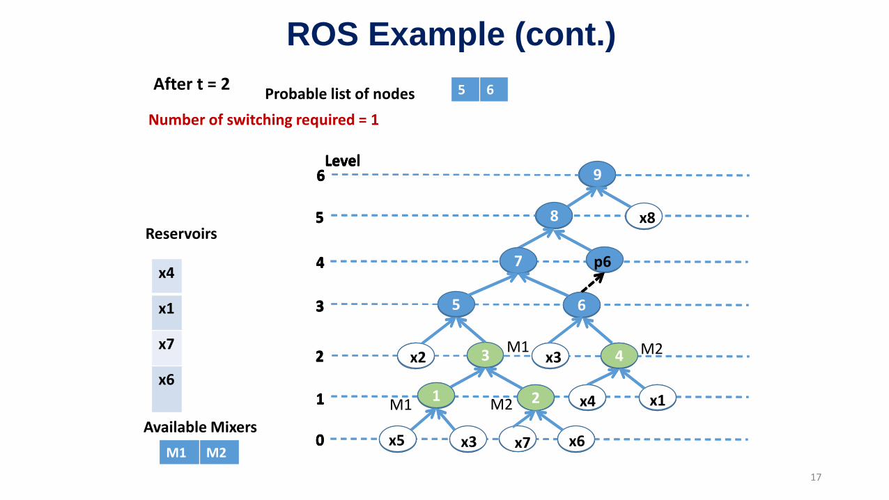
ROS Example (cont.)
9
8
7
5 6
3 4
1 2
x5 x3 x7 x6
x3
x4 x1
x2
x8
p6
Level6
5
4
3
2
1
0
After t = 2Probable list of nodes
Reservoirs
Available Mixers
9
8
7
5 6
3 4
1 2
x5 x3 x7 x6
x3
x4 x1
x2
x8
p6
Level6
5
4
3
2
1
0
x5
x3
x7
x6
9
8
7
5 6
3 4
1 2
x5 x3 x7 x6
x3
x4 x1
x2
x8
p6
Level6
5
4
3
2
1
0
3 4
x4
x1
x7
x6
Number of switching required = 1
M1 M2
M1 M2
5 6
x4
x1
x7
x6
M1 M2
17

ROS Example (cont.)
9
8
7
5 6
3 4
1 2
x5 x3 x7 x6
x3
x4 x1
x2
x8
p6
Level6
5
4
3
2
1
0
At t = 3Probable list of nodes
Reservoirs
Available Mixers
9
8
7
5 6
3 4
1 2
x5 x3 x7 x6
x3
x4 x1
x2
x8
p6
Level6
5
4
3
2
1
0
x5
x3
x7
x6
9
8
7
5 6
3 4
1 2
x5 x3 x7 x6
x3
x4 x1
x2
x8
p6
Level6
5
4
3
2
1
0
3 4
x4
x1
x7
x6
Number of switching required = 2
M1 M2
M1 M2
5 6
x4
x1
x7
x6
9
8
7
5 6
3 4
1 2
x5 x3 x7 x6
x3
x4 x1
x2
x8
p6
Level6
5
4
3
2
1
0
5 6
x2
x3
x7
x6
M1 M2
7
18

ROS Example (cont.)
9
8
7
5 6
3 4
1 2
x5 x3 x7 x6
x3
x4 x1
x2
x8
p6
Level6
5
4
3
2
1
0
At t = 4Probable list of nodes
Reservoirs
Available Mixers
9
8
7
5 6
3 4
1 2
x5 x3 x7 x6
x3
x4 x1
x2
x8
p6
Level6
5
4
3
2
1
0
x5
x3
x7
x6
9
8
7
5 6
3 4
1 2
x5 x3 x7 x6
x3
x4 x1
x2
x8
p6
Level6
5
4
3
2
1
0
x4
x1
x7
x6
Number of switching required = 2
M1 M2
M1 M2
5
x4
x1
x7
x6
9
8
7
5 6
3 4
1 2
x5 x3 x7 x6
x3
x4 x1
x2
x8
p6
Level6
5
4
3
2
1
0
x2
x3
x7
x6
M1 M2
7
9
8
7
5 6
3 4
1 2
x5 x3 x7 x6
x3
x4 x1
x2
x8
p6
Level6
5
4
3
2
1
0
7
x2
x3
x7
x6
M2
8
M1
19

ROS Example (cont.)
9
8
7
5 6
3 4
1 2
x5 x3 x7 x6
x3
x4 x1
x2
x8
p6
Level6
5
4
3
2
1
0
At t = 5Probable list of nodes
Reservoirs
Available Mixers
9
8
7
5 6
3 4
1 2
x5 x3 x7 x6
x3
x4 x1
x2
x8
p6
Level6
5
4
3
2
1
0
x5
x3
x7
x6
9
8
7
5 6
3 4
1 2
x5 x3 x7 x6
x3
x4 x1
x2
x8
p6
Level6
5
4
3
2
1
0
x4
x1
x7
x6
Number of switching required = 2
M1 M2
M1 M2
5
x4
x1
x7
x6
9
8
7
5 6
3 4
1 2
x5 x3 x7 x6
x3
x4 x1
x2
x8
p6
Level6
5
4
3
2
1
0
x2
x3
x7
x6
M1 M2
7
9
8
7
5 6
3 4
1 2
x5 x3 x7 x6
x3
x4 x1
x2
x8
p6
Level6
5
4
3
2
1
0
8
x2
x3
x7
x6
M2
9
M1
M1
20

ROS Example (cont.)
9
8
7
5 6
3 4
1 2
x5 x3 x7 x6
x3
x4 x1
x2
x8
p6
Level6
5
4
3
2
1
0
At t = 6Probable list of nodes
Reservoirs
Available Mixers
9
8
7
5 6
3 4
1 2
x5 x3 x7 x6
x3
x4 x1
x2
x8
p6
Level6
5
4
3
2
1
0
x5
x3
x7
x6
9
8
7
5 6
3 4
1 2
x5 x3 x7 x6
x3
x4 x1
x2
x8
p6
Level6
5
4
3
2
1
0
x4
x1
x7
x6
Number of switching required = 3
M1 M2
M1 M2
5
x4
x1
x7
x6
9
8
7
5 6
3 4
1 2
x5 x3 x7 x6
x3
x4 x1
x2
x8
p6
Level6
5
4
3
2
1
0
x2
x3
x7
x6
M1 M2
9
8
7
5 6
3 4
1 2
x5 x3 x7 x6
x3
x4 x1
x2
x8
p6
Level6
5
4
3
2
1
0
9
x8
x3
x7
x6
M2
M1
M1
M1
21

ROS Example (cont.)
9
8
7
5 6
3 4
1 2
x5 x3 x7 x6
x3
x4 x1
x2
x8
p6
Level6
5
4
3
2
1
0
Total Mixing time = 6
M1 M2
Number of switching required = 3
M1M2
M1 M2
M1
M1
M1
22

Reservoir and Mixer Constrained Scheduling (RMS)
• In ROS, the priority is given to reducing the mixing time ratherthan reservoir switching
• But reservoir switching takes more time than mixing [Rensch et al.,Lab Chip, 2014]
• In RMS, reducing reservoir switching is main objective
23

Problem Formulation- RMS
• Inputs: Mixing tree (T), number of mixers available (NM) and number ofreservoirs available (NR)
• Output: Scheduled mixing tree and total mixing time (Tm)
• Constraints:• Number of reservoirs used at any time t, NR
• Number of mixers used at any time t, NM
• Objectives:• Minimize the number of switching (S)
• Minimize the total mixing time (Tm)
24

Proposed Scheme - RMS
1. Approximate given target ratio at accuracy level d
3. The dynamic list is sorted in decreasing order of (ci)’s and inwhich the reagent’s priorities are set in increasing order
4. A probable list is created which contains the intermediate nodesthat can be scheduled at the current time
2. Create a dynamic list (D = {xi(ci)}), where xi represents thereagent i and ci/2
d is the target concentration of xi
25

RMS (cont.)
• Both Reservoirs are empty.
• If reagents of current node is not loaded, then load them
Case -1
• Reservoirs are loaded.
• Switch the reagents, if it has high priority
Case -2
• For each node and current reservoir following cases may occur:
26

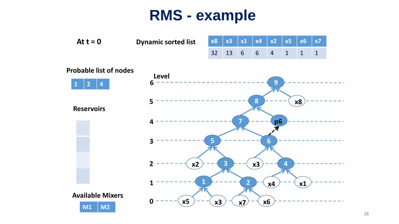
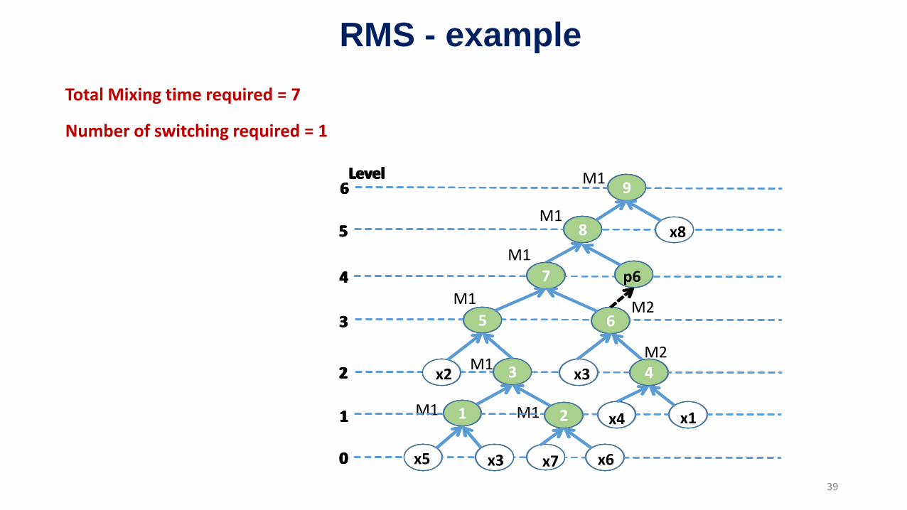
RMS - example
• Given a following CoDOS tree with target ratio 500 : 300 : 1000 : 500 : 100 : 100 : 25 : 2475 (approximated as 6 : 4 : 13 : 6 : 1 : 1 : 1 : 32 in 64-scale)
• Consider the DMFB architecture with 2 mixers and 4 reservoirs given below
9
8
7
5 6
3 4
1 2
x5 x3 x7 x6
x3
x4 x1
x2
x8
p6
Level6
5
4
3
2
1
0
Schedule for NM = 2 and NR = 4
Initial Dynamic sorted listx8 x3 x1 x4 x2 x5 x6 x7
32 13 6 6 4 1 1 1
Initial Probable list of nodes 1 2 4
27
RMS - example
9
8
7
5 6
3 4
1 2
x5 x3 x7 x6
x3
x4 x1
x2
x8
p6
Level6
5
4
3
2
1
0
At t = 0 Dynamic sorted list x8 x3 x1 x4 x2 x5 x6 x7
32 13 6 6 4 1 1 1
Probable list of nodes
1 2 4
Reservoirs
Available Mixers
M1 M228

RMS - example
9
8
7
5 6
3 4
1 2
x5 x3 x7 x6
x3
x4 x1
x2
x8
p6
Level6
5
4
3
2
1
0
At t = 1 Dynamic sorted list
Probable list of nodes
1 2 4
Reservoirs
Available Mixers
9
8
7
5 6
3 4
2
x5 x3 x7 x6
x3
x4 x1
x2
x8
p6
Level6
5
4
3
2
1
0
Dynamic sorted list x8 x3 x1 x4 x2 x5 x6 x7
32 13 6 6 4 1 1 1
Probable list of nodes
1 2 4
x6
x7
Reservoirs
0
Available Mixers
M2
0
M1
29

RMS - example
9
8
7
5 6
3 4
1 2
x5 x3 x7 x6
x3
x4 x1
x2
x8
p6
Level6
5
4
3
2
1
0
At t = 1 Dynamic sorted list
Probable list of nodes
1 2 4
Reservoirs
Available Mixers
9
8
7
5 6
3 4
2
x5 x3 x7 x6
x3
x4 x1
x2
x8
p6
Level6
5
4
3
2
1
0
M1
M2
Dynamic sorted list x8 x3 x1 x4 x2 x5 x6 x7
32 13 6 6 4 1 1 1
1 2 4
x6
x7
x1
x4
Reservoirs
0
Available Mixers
000
30

RMS - example
9
8
7
5 6
3 4
1 2
x5 x3 x7 x6
x3
x4 x1
x2
x8
p6
Level6
5
4
3
2
1
0
After t = 1 Dynamic sorted list
Probable list of nodes
Reservoirs
Available Mixers
M1 M2
9
8
7
5 6
3 4
2
x5 x3 x7 x6
x3
x4 x1
x2
x8
p6
Level6
5
4
3
2
1
0
x8 x3 x2 x5 x1 x4 x6 x7
32 13 4 1 0 0 0 0
1 6
x6
x7
x1
x4
M1 M2
M1
M2
31

RMS - example
9
8
7
5 6
3 4
1 2
x5 x3 x7 x6
x3
x4 x1
x2
x8
p6
Level6
5
4
3
2
1
0
At t = 2 Dynamic sorted list
Probable list of nodes
Reservoirs
Available Mixers
9
8
7
5 6
3 4
2
x5 x3 x7 x6
x3
x4 x1
x2
x8
p6
Level6
5
4
3
2
1
0
1 6
x6
x7
x1
x4M1
9
8
7
5 6
3 4
1 2
x5 x3 x7 x6
x3
x4 x1
x2
x8
p6
Level6
5
4
3
2
1
0
x8 x3 x2 x5 x1 x4 x6 x7
32 13 4 1 0 0 0 0
1 6
x5
x3
x2
x8
M2
M1
M2
00Number of switching required = 1
32

RMS - example
9
8
7
5 6
3 4
1 2
x5 x3 x7 x6
x3
x4 x1
x2
x8
p6
Level6
5
4
3
2
1
0
After t = 2 Dynamic sorted list
Probable list of nodes
Reservoirs
Available Mixers
9
8
7
5 6
3 4
2
x5 x3 x7 x6
x3
x4 x1
x2
x8
p6
Level6
5
4
3
2
1
0
x6
x7
x1
x4M1
9
8
7
5 6
3 4
1 2
x5 x3 x7 x6
x3
x4 x1
x2
x8
p6
Level6
5
4
3
2
1
0
x5
x3
x2
x8
M2
M1
M2
Number of switching required = 1
x8 x2 x1 x3 x4 x5 x6 x7
32 4 0 0 0 0 0 0
3
M1 M233

RMS - example
9
8
7
5 6
3 4
1 2
x5 x3 x7 x6
x3
x4 x1
x2
x8
p6
Level6
5
4
3
2
1
0
At t = 3 Dynamic sorted list
Probable list of nodes
Reservoirs
Available Mixers
9
8
7
5 6
3 4
2
x5 x3 x7 x6
x3
x4 x1
x2
x8
p6
Level6
5
4
3
2
1
0
x6
x7
x1
x4M1
9
8
7
5 6
3 4
1 2
x5 x3 x7 x6
x3
x4 x1
x2
x8
p6
Level6
5
4
3
2
1
0
x5
x3
x2
x8
M2
M1
M2
Number of switching required = 1
x8 x2 x1 x3 x4 x5 x6 x7
32 4 0 0 0 0 0 0
3 9
8
7
5 6
3 4
1 2
x5 x3 x7 x6
x3
x4 x1
x2
x8
p6
Level6
5
4
3
2
1
0
3
M2
5
M1
34

RMS - example
9
8
7
5 6
3 4
1 2
x5 x3 x7 x6
x3
x4 x1
x2
x8
p6
Level6
5
4
3
2
1
0
At t = 4 Dynamic sorted list
Probable list of nodes
Reservoirs
Available Mixers
9
8
7
5 6
3 4
2
x5 x3 x7 x6
x3
x4 x1
x2
x8
p6
Level6
5
4
3
2
1
0
x6
x7
x1
x4M1
9
8
7
5 6
3 4
1 2
x5 x3 x7 x6
x3
x4 x1
x2
x8
p6
Level6
5
4
3
2
1
0
x5
x3
x2
x8
M2
M1
M2
Number of switching required = 1
3 9
8
7
5 6
3 4
1 2
x5 x3 x7 x6
x3
x4 x1
x2
x8
p6
Level6
5
4
3
2
1
0
5
M2
5
M1
9
8
7
5 6
3 4
1 2
x5 x3 x7 x6
x3
x4 x1
x2
x8
p6
Level6
5
4
3
2
1
0
x8 x2 x1 x3 x4 x5 x6 x7
32 4 0 0 0 0 0 0
x5
x3
x2
x8
7
M1
0
35

RMS - example
9
8
7
5 6
3 4
1 2
x5 x3 x7 x6
x3
x4 x1
x2
x8
p6
Level6
5
4
3
2
1
0
At t = 5 Dynamic sorted list
Probable list of nodes
Reservoirs
Available Mixers
9
8
7
5 6
3 4
2
x5 x3 x7 x6
x3
x4 x1
x2
x8
p6
Level6
5
4
3
2
1
0
x6
x7
x1
x4M1
9
8
7
5 6
3 4
1 2
x5 x3 x7 x6
x3
x4 x1
x2
x8
p6
Level6
5
4
3
2
1
0
x5
x3
x2
x8
M2
M1
M2
Number of switching required = 1
3 9
8
7
5 6
3 4
1 2
x5 x3 x7 x6
x3
x4 x1
x2
x8
p6
Level6
5
4
3
2
1
0
5
M2
5
M1
9
8
7
5 6
3 4
1 2
x5 x3 x7 x6
x3
x4 x1
x2
x8
p6
Level6
5
4
3
2
1
0
x5
x3
x2
x8
7
M1
9
8
7
5 6
3 4
1 2
x5 x3 x7 x6
x3
x4 x1
x2
x8
p6
Level6
5
4
3
2
1
0
x8 x1 x2 x3 x4 x5 x6 x7
32 0 0 0 0 0 0 0
7 8
M1
36
RMS - example
9
8
7
5 6
3 4
1 2
x5 x3 x7 x6
x3
x4 x1
x2
x8
p6
Level6
5
4
3
2
1
0
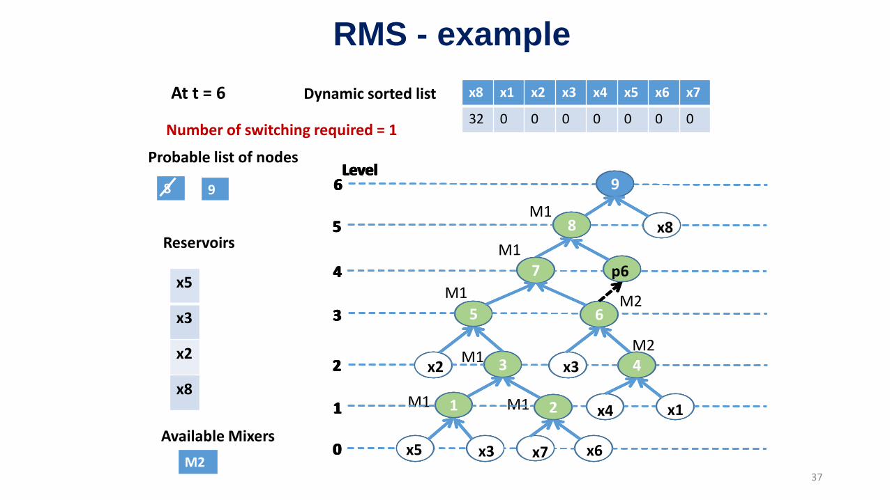
At t = 6 Dynamic sorted list
Probable list of nodes
Reservoirs
Available Mixers
9
8
7
5 6
3 4
2
x5 x3 x7 x6
x3
x4 x1
x2
x8
p6
Level6
5
4
3
2
1
0
x6
x7
x1
x4M1
9
8
7
5 6
3 4
1 2
x5 x3 x7 x6
x3
x4 x1
x2
x8
p6
Level6
5
4
3
2
1
0
x5
x3
x2
x8
M2
M1
M2
Number of switching required = 1
3 9
8
7
5 6
3 4
1 2
x5 x3 x7 x6
x3
x4 x1
x2
x8
p6
Level6
5
4
3
2
1
0
5
M2
5
M1
9
8
7
5 6
3 4
1 2
x5 x3 x7 x6
x3
x4 x1
x2
x8
p6
Level6
5
4
3
2
1
0
x5
x3
x2
x8
7
M1
9
8
7
5 6
3 4
1 2
x5 x3 x7 x6
x3
x4 x1
x2
x8
p6
Level6
5
4
3
2
1
0
7 8
M1
x8 x1 x2 x3 x4 x5 x6 x7
32 0 0 0 0 0 0 0
8 9
M1
37

RMS - example
9
8
7
5 6
3 4
1 2
x5 x3 x7 x6
x3
x4 x1
x2
x8
p6
Level6
5
4
3
2
1
0
At t = 7 Dynamic sorted list
Probable list of nodes
Reservoirs
Available Mixers
9
8
7
5 6
3 4
2
x5 x3 x7 x6
x3
x4 x1
x2
x8
p6
Level6
5
4
3
2
1
0
x6
x7
x1
x4M1
9
8
7
5 6
3 4
1 2
x5 x3 x7 x6
x3
x4 x1
x2
x8
p6
Level6
5
4
3
2
1
0
x5
x3
x2
x8
M2
M1
M2
Number of switching required = 1
3 9
8
7
5 6
3 4
1 2
x5 x3 x7 x6
x3
x4 x1
x2
x8
p6
Level6
5
4
3
2
1
0
5
M2
M1
9
8
7
5 6
3 4
1 2
x5 x3 x7 x6
x3
x4 x1
x2
x8
p6
Level6
5
4
3
2
1
0
x5
x3
x2
x8
M1
9
8
7
5 6
3 4
1 2
x5 x3 x7 x6
x3
x4 x1
x2
x8
p6
Level6
5
4
3
2
1
0
7
M1
x8 x1 x2 x3 x4 x5 x6 x7
32 0 0 0 0 0 0 0
9
M1
M1
0
38
RMS - example
9
8
7
5 6
3 4
1 2
x5 x3 x7 x6
x3
x4 x1
x2
x8
p6
Level6
5
4
3
2
1
0
9
8
7
5 6
3 4
2
x5 x3 x7 x6
x3
x4 x1
x2
x8
p6
Level6
5
4
3
2
1
0
M1
9
8
7
5 6
3 4
1 2
x5 x3 x7 x6
x3
x4 x1
x2
x8
p6
Level6
5
4
3
2
1
0
M2
M1
M2
9
8
7
5 6
3 4
1 2
x5 x3 x7 x6
x3
x4 x1
x2
x8
p6
Level6
5
4
3
2
1
0
M1
9
8
7
5 6
3 4
1 2
x5 x3 x7 x6
x3
x4 x1
x2
x8
p6
Level6
5
4
3
2
1
0
M1
9
8
7
5 6
3 4
1 2
x5 x3 x7 x6
x3
x4 x1
x2
x8
p6
Level6
5
4
3
2
1
0
M1
M1
M1
Total Mixing time required = 7
Number of switching required = 1
39

Comparison of number of switching by RMS and ROS for CoDOS, MinMix, RMA mixing Trees
Simulation Results
40
Test data set (10,000 ratios): http://faculty.iitr.ac.in/~sudiproy.fcs/codalab/research/microfluidics.html

Simulation Results (cont.)
Comparison of mixing time by RMS and ROS for CoDOS, MinMix, RMA mixing Trees
41
Test data set (10,000 ratios): http://faculty.iitr.ac.in/~sudiproy.fcs/codalab/research/microfluidics.html

Comparative results of RMS over ROS for some example ratios used in real-life bioprotocols
Simulation Results (cont.)
42

Conclusions and Future Work
• Reservoir switching is required when number of reagents are morethan reservoirs
• Reservoir switching requires more time than other fluidic operations
• RMS can reduce the number of switching as compared to ROSschemes with slight increase in mixing time
• As a future work, reducing the storage requirement can also beadded to the optimization criteria
43

References
[1] K. Chakrabarty and F. Su, Digital Microfluidic Biochips: Synthesis, Testing and Reconfiguration Techniques. CRCPress, 2007.
[2] Y.-L. Hsieh, T.-Y. Ho, and K. Chakrabarty, “A Reagent-Saving Mixing Algorithm for Preparing Multiple-TargetBiochemical Samples Using Digital Microfluidics,” IEEE Transactions on Computer-Aided Design of IntegratedCircuits and Systems (TCAD), vol. 31, no. 11, pp. 1656–1669, 2012.
[3] S. Roy, B. B. Bhattacharya, and K. Chakrabarty, “Optimization of Dilution and Mixing of Biochemical Samplesusing Digital Microfluidic Biochips,” IEEE Transactions on Computer-Aided Design of Integrated Circuits and Systems(TCAD), vol. 29, no. 11, pp. 1696–1708, 2010.
[4] W. Thies, J. P. Urbanski, T. Thorsen, and S. Amarasinghe, “Abstraction Layers for Scalable MicrofluidicBiocomputing,” Natural Computing, vol. 7, no. 2, pp. 255– 275, 2008.
[5] C.-H. Liu, H.-H. Chang, T.-C. Liang, and J.-D. Huang, “Sample Preparation for Many-Reactant Bioassay on DMFBsusing Common Dilution Operation Sharing,” in Proc. of the IEEE/ACM International Conference on Computer-AidedDesign (ICCAD), 2013, pp. 615–621.
44

References[6] S. Kumar, S. Roy, P. P. Chakrabarti, B. B. Bhattacharya, and K. Chakrabarty, “Efficient Mixture Preparation on DigitalMicrofluidic Biochips,” in Proc. of the IEEE International Symposium on Design and Diagnostics of Electronic CircuitsSystems (DDECS), 2013, pp. 205–210.
[7] S. Roy, B. B. Bhattacharya, S. Ghoshal, and K. Chakrabarty, “Theory and Analysis of Generalized Mixing andDilution of Biochemical Fluids Using Digital Microfluidic Biochips,” ACM Journal on Emerging Technologies inComputing Systems (JETC), vol. 11, no. 1, pp. 2.1–2.33, 2014.
[8] S. Roy, P. P. Chakrabarti, S. Kuamr, K. Chakrabarty, and B. B. Bhattacharya, “Layout-Aware Mixture Preparation ofBiochemical Fluids on Application-Specific Digital Microfluidic Biochips,” ACM Transactions on Design Automation ofElectronic Systems (TODAES), vol. 20, no. 3, pp. 45.1–45.34, 2015.
[9] F. Su and K. Chakrabarty, “Architectural-Level Synthesis of Digital Microfluidicsbased Biochips,” in Proc. of theIEEE/ACM International Conference on Computer- Aided Design (ICCAD), 2004, pp. 223–228.
[10] L. Luo and S. Akella, “Optimal Scheduling of Biochemical Analyses on Digital Microfluidic Systems,” IEEETransactions on Automation Science and Engineering (TASE), vol. 8, no. 1, pp. 216–227, 2011.
[11] D. Grissom and P. Brisk, “Path scheduling on Digital Microfluidic Biochips,” in Proc. of the IEEE/ACM DesignAutomation Conference (DAC), 2012, pp. 26–35.
45

References
[12] S. Srigunapalan, I. A. Eydelnant, C. A. Simmons, and A. R. Wheeler, “A Digital Microfluidic Platform for PrimaryCell Culture and Analysis,” Lab Chip, vol. 12, pp. 369–375, 2012.
[13] P. Y. Paik, V. K. Pamula, M. G. Pollack, and R. B. Fair, “Electrowetting-Based Droplet Mixers for MicrofluidicSystems,” Lab Chip, vol. 3, no. 1, pp. 28–33, 2003.
[14] C. Rensch, S. Lindner, R. Salvamoser, S. Leidner, C. Bold, V. Samper, D. Taylor, M. Baller, S. Riese, P. Bartenstein, C.Wangler, and B. Wangler, “A Solvent Resistant Lab-on-Chip Platform for Radiochemistry Applications,” Lab Chip, vol.14, pp. 2556–2564, 2014.
[15] Preparation of Plasmid DNA by Alkaline Lysis with SDS: Minipreparation, Cold Spring Harb Protocols,http://cshprotocols.cshlp.org/content/2006/1/pdb.prot4084.citation, 2006.
[16] A. G. Uren, H. Mikkers, J. Kool, L. van der Weyden, A. H. Lund, C. H. Wilson, R. Rance, J. Jonkers, M. vanLohuizen, A. Berns, and D. J. Adams, “A High- Throughput Splinkerette-PCR Method for the Isolation and Sequencingof Retroviral Insertion Sites,” Nature Protocols, vol. 4, no. 5, pp. 789–798, 2009.
[17] OpenWetWare, 2009, http://openwetware.org/wiki/Main Page.
46

Thank You
47
Any Questions?