reserves, liquidity and money: an assessment of balance ... · 304 bis papers no 66 reserves,...

304 BIS Papers No 66

Reserves, liquidity and money: an assessment of balance sheet policies1

Jagjit S Chadha,2 Luisa Corrado3 and Jack Meaning4

Abstract

The financial crisis and its aftermath have stimulated a vigorous debate on the use of macro-prudential instruments both for regulating the banking system and for providing additional tools for monetary policymakers. The widespread adoption of non-conventional monetary policies has provided some evidence on the efficacy of liquidity and asset purchases for offsetting the zero lower bound. Central banks have thus been put in mind of the effectiveness of extended open market operations as supplementary monetary policy tools. These are essentially fiscal instruments, in that they entail the issuance of central bank liabilities backed by fiscal transfers. Given that these tools are written into fiscal budget constraints, we can examine the consequences of the operations in the context of a micro-founded macroeconomic model of banking and money, and we can simulate the responses of the Federal Reserve balance sheet to the crisis. Specifically, we examine the role that reserves for bond and capital swaps play in stabilising the economy, as well as the impact of changes in the composition of the central bank balance sheet. We find that such policies can significantly enhance the ability of the central bank to stabilise the economy. This is because balance sheet operations supply (remove) liquidity to a financial market that is otherwise short (long) of liquidity, and hence allow other financial spreads to move less violently over the cycle to compensate.

Keywords: Non-conventional monetary interest on reserves, monetary and fiscal policy instruments, Basel III

JEL classification: E31, E40, E51

1 This version of the paper dates from December 2011. An earlier version of this paper was presented at the

Bank for International Settlements, at the Bundesbank, at the ECB and at the Bank of Greece, as well as the University of Cambridge, University of Kent, University of Oxford, University of York and the FSA. Our thanks go to Steve Cecchetti, Alec Chrystal, Harris Dellas, Andrew Filardo, Christina Gerberding, Rafael Gerke, Charles Goodhart, Mar Gudmundsson, Norbert Janssen, Thomas Laubach, Paul Levine, Richard Mash, Patrick Minford, Marcus Miller, Richhild Moessner, Joe Pearlman, Peter Sinclair and Peter Spencer for helpful comments, and in particular to the participants at the joint Bank of Thailand-BIS conference on central bank balance sheets.

2 Professor of Economics, Chair in Banking and Finance, School of Economics, Keynes College, University of Kent, Canterbury, UK, CT2 9LP. E-mail: [email protected]. Centre for International Macroeconomics and Finance, University of Cambridge.

3 Associate Professor of Economics, Department of Economics, University of Rome, Tor Vergata. E-mail: [email protected].

4 School of Economics, Keynes College, University of Kent, Canterbury, UK, CT2 9LP. E-mail: [email protected].

BIS Papers No 66 305

1. Introduction

The on-going financial and credit crisis has pushed existing monetary policy practices to their limit and created considerable interest in identifying an appropriate post-crisis operating framework for monetary policy, particularly as there has been an active parallel debate about the regulatory framework for commercial banking. What might ultimately be termed the first generation of micro-founded monetary policy models had little to say about the new monetary policy frameworks, since the short-term policy rate was sufficient to stabilise the economy. But during this crisis many types of extended open market operations have been used in efforts to affect longer-term interest rates and asset prices, given that the short-term rate was constrained at the zero lower bound. Thus, in this paper we seek to address the question of post-crisis monetary policy by considering the role of balance sheet operations in a model in which commercial banks, lending and external finance premia all affect the optimal formulation of monetary policy.

The Goodfriend-McCallum (2007) model represents a Calvo-Yun monopolistically competitive production economy with sticky prices, where households respect their budget constraints in planning consumption, but where households must hold bank deposits to effect transactions. Hence, loan technology for the banking sector takes centre stage in this model,5 which addresses the requirements of the private sector subject to monitoring and quality of collateral constraints. Households can work either in the goods producing sector or in the banking sector monitoring loan quality. But in order to consider the implications of reserves, in the version of the model developed by Chadha and Corrado (2011) banks also have to make a choice regarding their asset mix in terms of reserves with the central bank versus loans with the private sector. The central bank in this model holds commercial bank reserves and sets the interest rate paid on them, and the government budget constraint is modified to include claims from reserves, as well as standard issuance of public debt to meet excess of expenditures over taxes. Reserves in this model are outside money and respond to the demand for liquidity from financial institutions.

A banking-sector-based model can both amplify and add persistence to a standard macroeconomic setup. This is because decision rules for output are shown to incorporate the equilibrium level of commercial bank assets and the price (or spread) at which those assets are provided. The recent boom and bust in advanced country debtor economies would seem to confirm the continuing relevance of this insight. First, we consider the non-standard monetary, or balance sheet, policies carried out by the Federal Reserve in response to the financial crisis, and examine how they can be modelled. Specifically, we model the injection of bank reserves in our model economy in three ways, either as a perfectly elastic supply of bank reserves meeting commercial bank demand, or as a swap for bonds or capital. Furthermore we consider the role of a policy rule for the supply of reserves to supplement or replace existing interest rate rules. It is shown that these one-off responses can stabilise the economy following a negative downward shock to asset prices.

The motivation for providing reserves is to address the liquidity preference for commercial banks. Gale (2011) shows that, given risk aversion, the market cannot supply sufficient liquidity to the financial system. This is because there is an incentive for savers to swap illiquid assets for liquid assets, which will leave the market as a whole short of liquid assets and long illiquid assets. The problem will tend to be exacerbated if there is a collapse in confidence in the interbank market, when distributional shocks to banks no longer get recycled around the system. Monetary authorities can offset this liquidity shortage by issuing short-term liabilities backed by fiscal transfers, ie interest bearing reserves or T-bills. This

5 See Goodfriend and McCallum (2007) and Chadha, Corrado and Holly (2008) for an outline of this modelling

device and its implications.


operation reduces private sector holdings of illiquid assets and increases the banking sector’s reserve-deposit ratio. From a fiscal or debt management perspective, if we take the structure of debt as given, the swap of illiquid for liquid debt instruments hedges the private sector against liquidity risk and allows the fiscal policymaker to collect a return in the form of liquidity premia. The danger of the operation is that it is conducted at a time of fiscal deficits and so may be viewed as a change in the preferences of the monetary and fiscal policymaker, and thus lead to an expectation of lower interest rates and higher fiscal deficits (see Nordhaus, 1994).

Under the condition of coordination of monetary and fiscal policy, we can examine the case for the systematic use of balance sheet or reserve policies. For in contrast to a model that does not explicitly model bank balance sheets, this model can deliver an endogenous dynamic response for various risk premia and for the supply of loans and deposits. Using standard methods, we can also compare the responses of our artificial economy with and without reserve injections. We derive the approximate welfare criterion of the representative household and find that the economy in which commercial banks have an endogenous choice over reserve holdings (qua liquidity) performs better in welfare terms than an economy where commercial banks lack such an incentive. The holding of reserves over the business cycle acts as a substitute for more costly provision of commercial bank assets, and thus reduces the volatility of interest spreads in shock scenarios. Also, by varying the availability of reserves over expansions and contractions, it helps to stabilize the impulse from the monetary sector.6

The structure of this paper is as follows. Section 2 outlines by way of example the unconventional monetary policies of the Federal Reserve, and uses a simple framework for understanding a stylized flow of funds and the role of commercial banks in the monetary system. Our setup also incorporates the government's budget constraint in this section, showing that the payment of the policy rate on bank reserves will have a direct impact on the equation of motion for government debt. Section 3 sketches the implications of the loan production function approach for key macroeconomic decision rules, and outlines the determination of key market interest rates. Section 4 considers the implications of commercial banks’ asset management in terms of reserve holdings, to account for the relative returns from holding reserves or producing loans and for liquidity concerns. Section 5 explains the standard calibration techniques used. Section 6 outlines the results of the impulse response analysis of various balance sheet operations, and undertakes welfare analysis of some key results. Section 7 presents conclusions and some final observations.

2. Unconventional Monetary Policy in the U.S.

The outbreak of the financial crisis in the U.S housing market in early 2007 and the way it spread to a full-blown, global financial meltdown by 2008 are well documented. In response to immense contractionary pressure, the Federal Reserve, like many other central banks the world over, cut its policy rate quickly and dramatically. The target federal funds rate fell from 5.25% in September 2007 to between 0% and 0.25% by January 2009, effectively reaching the zero lower bound (ZLB). With short-term nominal interest rates constrained, what was previously a largely theoretical discussion of how to gain traction for monetary policy at the ZLB became a real and practical problem. The Federal Reserve embarked on a number of unconventional policy initiatives in order to provide monetary stimulus to the U.S economy and reactivate frozen credit markets. Many of these measures were concerned directly with the Fed's balance sheet, reserves and asset holdings. These policies at the ZLB are

6 Paying interest on reserves is thus a way to meet the Friedmanite maximum without deflation.


effectively fiscal policies, since they involve the issuance of short-term fiscal instruments, and hence we wish to integrate these monetary/fiscal instruments into our model.

2.1 Paying Interest on Reserves An initial but important policy development was the payment of interest on reserves held by commercial banks at the central bank. The Federal Reserve had applied to Congress for the authority to pay interest on bank reserves on various occasions (Meyer, 2001; Kohn, 2004) and was granted permission in 2006 under the Financial Services Regulatory Relief Act. Originally, the policy was not due to become effective until 2011, as Congress had worries about its fiscal costs,7 but as the economic conditions in the U.S. worsened, implementation was brought forward to 2008. There is strong theoretical backing for such a policy. Hall (2002) outlines a model in which the payment of interest on reserves can become a policy tool capable of controlling the price level in a world without money, whilst Chadha and Corrado (2011) show that paying interest on reserves at the policy rate can provide an incentive for financial intermediaries to vary their holdings of reserves cyclically, which in turn attenuates fluctuations in the external finance premium and helps stabilise the monetary economy. The issuance of such reserves is very close substitute for short-term T-bills, and because interest is payable these operations are in effect a swap of liquid assets for illiquid assets.

2.2 Large Scale Asset Purchases Large Scale Asset Purchases (LSAPs) can be thought of as traditional open market operations in which the central bank changes the monetary base by buying and selling assets in exchange for reserves, but on a much larger scale and over a longer duration. Traditionally the central bank would use OMOs to meet the demand for reserves at its target interest rate, requiring relatively small, short-lived fluctuations in the level of reserves. In November 2008, the Fed announced that it would begin purchasing housing agency debt and mortgage-backed agency securities in the amount of $600bn in response to the housing crisis, and in order to promote the health of mortgage lending. In March 2009, this was increased to $1.25 trillion. The purchases were largely of maturities ranging from 3 months and 5 years. As they have reached maturity, principal has been reinvested to fund the purchase of Treasury securities and maintain the value of the agency debt and agency-backed securities section of the LSAP.

Accompanying this extension was the announcement that the Fed would begin to buy $300bn of Treasury securities, over 60% of which had maturities of 3 to 10 years. The purchase of Treasuries was designed to support falling asset prices by making the Fed present as a large buyer, and through the portfolio balance channel this was to spread to other assets in the economy. It also constituted a direct injection of liquid reserves into the economy to improve confidence and conditions in impaired credit markets. These large scale asset purchases were predominantly funded by the creation of over a trillion dollars of new reserves, making them the largest quantitative easing programme enacted since the crisis. In November 2010, in light of the continuing weakness predicted by economic forecasts, the purchase of longer-term Treasuries was extended by $600bn more under a second round of

7 Estimates by the Congressional Budget Office on the cost of paying interest suggest that the cost in the first

year would be $253 million, and that this would rise to $308 million by the fifth year, with a total of $1.4 billion over five years. This is based on the assumption that the federal funds rate would average 4.5% from 2008 to 2016, and that the Fed would pay interest at a rate 0.1 to 0.15 percentage points below that. It projected required reserves of about $8.3 billion. If the Fed only paid interest on excess reserves held, then the cost would be considerably smaller, though it would rise if commercial banks made more use of the facility. See Goodfriend (2002) for a recent survey.


quantitative easing (QE2), which took the total LSAP to over $2 trillion. In September 2011, the FOMC announced a maturity extension programme under which it is to buy an additional $400bn of longer-dated treasuries but simultaneously sterilise these by selling short-term Treasuries in the same amount. The goal is to lower longer-term yields without increasing the size of the central bank's balance sheet, by “twisting” the yield curve and increasing the average maturity of the Fed's Treasuries portfolio by 25 months. More may follow.

2.3 Other Policies

2.3.1 Commercial Paper Funding Facility One symptom of the financial crisis was the drying up of liquidity and a scarcity of available credit. This caused interest rates in commercial paper markets to rise, and the term that issuers of commercial paper could borrow shortened as investors moved away from longer-dated maturities in the face of uncertainty. In order to alleviate this situation, the Fed on 27 October 2008 began buying up high-rated, unsecured and asset-backed commercial paper through a special purpose vehicle, under financing provided by the Federal Reserve Bank of New York. The purchases were of newly issued, non-interest-paying 3-month-maturity commercial paper instruments, which were held for the full term, with the proceeds being used to repay the loan taken from the FRBNY to fund the original purchase. The CPFF was designed to realize the Fed's role as lender of last resort, assuring investors and issuers that firms would be able to meet their financing needs, and thus making them a more attractive investment and instilling confidence in credit markets. By easing liquidity pressure on firms and financial intermediaries, this could then also ease credit restrictions on households and businesses. After two extensions, the CPFF expired on 1 February 2010. At its largest, in January 2009, the facility held around $350bn of commercial paper, approximately two thirds of which was unsecured.8

2.3.2 TALF Following the collapse of Lehman Brothers in September 2008, the already strained asset-backed securities (ABS) market froze, with interest rate spreads soaring. ABS markets are one of the key drivers of funding to the wider economy, supplying credit for all manner of activity to consumers and businesses. With this in mind, on 25 November 2008 the FRBNY announced that in order to support the issuance of ABS, borrowers would be able to request non-recourse loans of 3- or 5-year duration against AAA-rated ABS through the Term Asset-Backed Securities Loan Facility (TALF).9 Initially the facility was granted permission to extend $200bn of loans, but with demand less than anticipated, only $70bn was actually lent while TALF was operational. Borrowers were eager to rid themselves of TALF financing since it came at a penalty. Thus, as conditions in credit markets improved, many paid back TALF loans early, securing funds privately. Because of this, the level of TALF credit currently outstanding is under $1bn. The non-recourse nature of these loans means that if the borrower cannot repay the loan, the collateral behind it, which can range from student loans and credit cards to small business loans or loans on commercial property, can be claimed by the Fed and sold. This had important implications for the risk faced by the Fed, helping to mitigate much of the risk that it could potentially incur by fulfilling this lender-of-last-resort role.

8 For a more in-depth discussion of the CPFF, see www.newyorkfed.org/research/epr/11v17n1/1105adri.pdf. 9 For a fuller description and analysis of TALF, see Brian Sack’s speech "Reflections on the TALF and the

Federal Reserve's Role as Liquidity Provider", available at http://www.newyorkfed.org/newsevents /speeches/2010/sac100609.html.

http://www.newyorkfed.org/newsevents%20/speeches/2010/sac100609.html

http://www.newyorkfed.org/newsevents%20/speeches/2010/sac100609.html


2.3.3 TARP The Federal Reserve was supported in its response to the crisis by the Treasury, which enacted a range of stimulus measures collectively dubbed the Troubled Asset Relief Programme (TARP). TARP consisted of a number of programmes, including $80bn of capital injections to U.S. automotive companies and $48bn to insurer AIG. The Treasury also provided credit protection totalling 10% of the Fed's TALF programme. By far the largest initiative in TARP was the Capital Purchase Programme (CaPP), which was launched on 14 October 2008 and accounted for over half of total TARP spending. Under CaPP, $250bn was extended by the Treasury to bolster the capital position of financially important firms. The elevated incidence of write-offs, defaults and under-performing loans which characterised the crisis left many financial intermediaries in a weakened capital position, negatively affecting their ability to extend credit and loans to the wider economy. This generated a loss of confidence in the institutions themselves, compounding the problem. CaPP sought to directly inject new capital into these organisations by purchasing preferred stock or securitised debt on which it received a dividend rate of roughly 5%. CaPP has provided a capital boost to 707 companies in the U.S., for a total of $205bn, but it has also received over $150bn in repayments as firms have found it possible to raise capital in the improved private markets and have paid back CaPP funds.

2.4 Credit Versus Quantitative Easing The term quantitative easing first appeared in the lexicon to describe the Bank of Japan's policy of central bank reserve creation when it found itself constrained by the zero lower bound to the policy rate in the early 2000s. In a speech at the London School of Economics in January 2009, Federal Reserve Chairman Ben Bernanke tried to distance the unconventional policy of the Fed in 2007 from this largely unsuccessful policy by saying:

In a pure QE regime, the focus of policy is the quantity of bank reserves, which are liabilities of the central bank; the composition of loans and securities on the asset side of the central bank's balance sheet is incidental.... In contrast, the Federal Reserve's credit easing approach focuses on the mix of loans and securities that it holds and on how this composition of assets affects credit conditions for households and businesses.

In theory, QE is a policy which seeks to change the size of the central bank's balance sheet, increasing liabilities through the creation of new reserves or other liquid fiscal liabilities. Often these reserves are then used to purchases assets from the financial or private sector. Credit easing (CE) differs in that it targets the asset side of the balance sheet, specifically the compositional mix of assets held by the central bank. In pure CE, the level of reserves and the subsequent size of the central bank's balance sheet do not change. In practice, most central banks' reactions to the crisis, including the Fed's, have elements of both quantitative and credit easing. In early 2008, the Fed began purchasing illiquid assets from private markets via liquidity swaps and the Term Auction Credit (TAC) programme, which it sterilised by selling its holdings of more liquid Treasury securities. Figure 1 shows that Fed holdings of U.S. Treasury securities fell from around $780bn in December 2007 to just $479bn by June 2008. This can be thought of as pure credit easing, as the sales of T-bills almost exactly offset the asset purchases, and the size of the balance sheet remained unaffected around $900bn, whilst reserves continued to be a tiny 0.01% of GDP. When the crisis worsened following the collapse of Lehman Brothers in September 2008, the Fed increased the provision of liquidity swaps and TAC, as well as introducing the CPFF and providing direct support to a number of systemically important institutions. Figure 1 shows that the Fed’s holdings of Treasury securities remained relatively constant over this period. Figure 2 shows how these increased purchases were funded in two ways. One was the introduction of the Supplementary Treasury Financing Account (STFA), where the Treasury brought forward its borrowing to exceed its current need and deposited the excess funds with the Federal Reserve. The second, and ultimately much larger, source of funds came from the creation of


new reserves. These new, unsterilized purchases caused the Fed’s balance sheet to grow rapidly. The Fed had now moved into QE, though it continued to assert that it was solely focussed on providing liquidity through its mix of assets, and that the increase in the size of the balance sheet was an incidental by-product of its credit easing policy.

However, with the LSAPs funded almost entirely through the creation of new reserves,10 reserve holdings have increased by a factor of 158 from their previous level of around just $11bn in 2007 to $1.74tn, or 13% of GDP. Table 1 shows the consolidated balance sheet of all Federal Reserve Banks pre- and post-crisis to demonstrate the scale of the change. The central bank balance sheet is now 3 times the size it was in 2007, and reserves, which originally accounted for around 1.5% of the liabilities, now make up almost two thirds.

2.5 The Unconventional Policy Balance Sheet We introduce a simple framework for analysing the effect of unconventional policies on the monetary balance sheet. For simplicity, since we abstract from other forms of central bank money and concentrate on bank reserves alone in our model, high-powered money is identical to reserves. More traditionally, the central bank controls the stock of fiat money (outside money), and financial intermediaries create other forms of money, which are claims on the private sector. Since financial intermediation allows alternative assets to serve as money, it offers a close substitute to (outside) fiat money, and the ability of the central bank to determine the overall nominal level of expenditure depends on the relationship between outside and inside money. The central bank has a powerful tool to regulate financial intermediaries and to affect the quantity of money in circulation, namely reserves, which may be fractional, voluntary or both.11

We first look at the private sector's balance sheet. The private sector has three forms of assets: deposits, D, held at banks, some fraction of bonds, γB, issued by the government, and a fraction of total capital.12 Their liabilities are loans, D-r, provided by banks. The government sector has liabilities in the form of outstanding public debt, B, and assets, represented by the present discounted value of future taxation. The commercial banks' balance sheet liabilities are deposits, D. Some fraction of liabilities, r, is held as reserves, and

10 In November 2009, the Fed began reinvesting the returns it made on agency debt and other short-term assets

it had bought to partially fund its further purchases of longer-term Treasury securities. 11 See Freeman and Haslag (1996) and Sargent and Wallace (1985). 12 In this example we assume that the private sector is represented by households.


the rest, D–r, is available to be lent to the private sector. The central bank holds assets in the form of some fraction of government bonds, (1–γ)B, and a fraction of capital, (1–γk)K, with liabilities determined by central bank money, which are reserves in this model.13 The net assets of commercial banks and of the central bank are both zero. The private sector has net assets given by

0( )i

k iiD B K D r tγ γ β∞

=+ + − − +∑ , and thus, because (1 ) kr B Kγ γ= − + and

0i

iit Bβ∞

==∑ , we can see that net private sector assets are also zero.

This flow of funds shows the mechanism by which unconventional policies operate. The central bank can perform quantitative easing by increasing the size of its balance sheet. It does this by extending an increased level of reserves to commercial banks. This must be backed by increased holdings of either bonds or capital, which in turn must be bought from the private sector. Alternatively, credit easing is conducted through the composition of the balance sheet. With their liabilities unchanged, the central bank can buy capital from the private sector, increasing its own holdings. It funds these purchases by selling bonds back to the private sector, leaving the net effect on the size of both the central bank and private sector's assets at zero. Due to the differing properties of bonds and capital as collateral in our model's loan production function, this exchange has implications for levels of deposit demand, which we shall discuss later.

2.5.1 Reserves and the fiscal position How can paying interest on reserves change the fiscal position? It does so because paying interest rates on reserves will ultimately depend on the public sector's budget constraint. The per-period government budget constraint means that any excess of government expenditure, Gt, over tax receipts, Tt, and payment of interest on debt, 1 1

Bt tR Bγ+ + , and/or reserves, IB

t tR r , will be financed by the issuance of bonds or central bank money, given the consumption-goods price index, A

tP . Note that the interest paid to the private sector is BR and the interest

to commercial banks is IBR , which is the policy rate in our model. Hence if we look at the consolidated budget identity for the government sector we note that:14

1 1

1(1 ) (1 )t t t t

t A IB A A B At t t t t t

r r B Bg taxP R P P R P

γ γ− +

+

− = − + −+ +

. (1)

Thus, the government can finance its net expenditure by issuing government debt, Bγ , or by issuing reserves, rt. However if interest rates are paid on reserves they will become interest bearing and therefore comparable to government debt. Clearly, any excess government expenditure can be financed by issuing bonds to the private sector or by supplying reserves to commercial banks at a differentiated interest rate. We leave the determination of the relative interest rates to section 3.1. Since we assume a stationary level of debt in this model, there are no implications for fiscal solvency in this setup, as all deviations from a steady-state debt-to-GDP ratio are strictly temporary. In effect, we are conditioning the issuance of reserves on a given path of public debt, which we simply assume to be optimal save for liquidity considerations.

13 If we operate in an open economy, central bank assets would also include foreign exchange reserves, f

r . 14 In this setting, the government sector includes both the government and the Bank of England. We also

assume that high-powered money comprises only reserves, not coin.


3. The General Equilibrium Monetary Model

As pointed out by Kiyotaki and Moore (2001), money aggregates should be reconnected to general equilibrium models, as they affect consumption decisions of liquidity-constrained households and the spreads across several financial instruments and assets. Similarly, open market operations or balance sheet policies will affect loans and therefore consumption. A simple way to incorporate money and spreads into a general equilibrium setting is to study the banking sector proposed by Goodfriend and McCallum (2007), which we extend to simulate the responses of the Federal Reserve balance sheet to the crisis. Specifically, we examine the role of reserves for bond and capital swaps in stabilising the economy, as well as the impact of changes in the composition of the central bank balance sheet.

The Goodfriend and McCallum model complements the traditional accelerator effect (Bernanke et al, 1999) with an attenuator effect, which is present in the model because monitoring effort is drawn into the banking sector in response to expanding consumption, which is accompanied by an expansion of bank lending that raises the marginal cost of loans and the external finance premium (EFP).The main feature of the model is the inclusion of households, production and monetary authority, alongside a banking sector which lends subject to monitoring costs, quality of capital and the availability of reserves.

3.1 Households and the Production Sector Households are liquidity constrained and decide the amount of consumption and the amount of labour they wish to supply to the production sector and to the banking sector according to the utility function

00

[ log( ) (1 ) log(1 )]t s st t t

tU E c n mβ φ φ

∞

=

= + − − −∑ , (2)

where tc denotes real consumption, stn is the supply of labour in the goods sector, s

tm is the supply of monitoring work in the banking sector and φ denotes the weight of consumption in the utility function. They are subject to the budget constraint

11

11

(1 ) ( ) ( )

( ) 0(1 )

s s At t tt t t t t t tA A A

t t t

t tt t t t t t tA A B

t t t

B D Pq K w n m cP P PD Bw n m tax q K cP P R

θγδ

γ

−−

++

− + + + + + +Π

− + − − − − − =+ ,

(3)

where is the price of capital, is the quantity of capital, is the price of household's

produced good, is the consumption goods price index, is the labour demanded by household as producer, is the labour demanded by household’s banking operation, is the real wage, is the nominal holding of broad money, is the real lump-sum tax

payment, and is the nominal interest rate on government bonds purchased in year . We also assume that any profit from the banking sector, , goes to the

household sector. The Lagrange multiplier of this constraint is denoted as , and is the

elasticity of household demand. Households choose the level of monitoring work, tm , and the level of employment work, tn , that they wish to offer to the production sector and the banking sector.

At the same time households’ consumption, given the cash-in-advance constraint, is affected by the amount of loanable funds they can obtain:

tq tK tPA

tP tn

tm tw

tD ttaxBtR

11, tt B ++ tΠ

tλ θ


/ At t t tc v D P= , (4)

where tv denotes velocity and tD is deposits.

The production sector, characterized by monopolistic competition and Calvo pricing, adopts a standard Cobb-Douglas production function with capital tK , and labour tn , subject to productivity shocks. Firms decide the amount of production they wish to supply and the demand for labour, by equalizing sales to net production:

( )1( 1 ) / 0A At t t t t tK A n c P P

θη η −− − = , (5)

where η denotes the capital share in the firm production function, is a productivity shock in the goods production sector whose mean increases over time at a rate γ, and θ denotes the elasticity of aggregate demand, A

tc . The Lagrange multiplier of this constraint is denoted by tξ . By clearing the household and production sectors,15 we can define the equilibrium in the labour market and in the goods market. Specifically, the demand for monitoring work,

11t tt t t

m cc wφ αλ

−= − ,

(6)

depends negatively on wages, tw , and positively on consumption, tc , where 1 α− is the share of monitoring in the loan production function. These two sectors also provide the standard relationship for the riskless interest rate and the bond rate.

3.2 Banking Sector We now turn to the analysis of how the banking sector affects the economy. The production function for the quantity of loans is given by:

( ) ( )11 1/ 3 2 0 1At t t t t t t tL P F b A kq K A mα αγ α−

+ += + < < , (7)

where A2t denotes a shock to monitoring work, A3t is a shock to capital as collateral and ( )1 1 1/ 1A B

t t t tb B P R+ + += + . The parameter k denotes the inferiority of capital as collateral in the banking production function, while α is the share of collateral in the loan production function. Increasing monitoring effort is achieved by increasing the number of people employed in the banking sector and thereby reducing employment in the goods production sector.

While in standard Calvo-Yun models nominal consumption plans pin down the demand for money, in this model with banking, money is produced by banks, so any shift in the supply of lendable funds generated by shocks to monitoring effort or collateral also affects consumption. Specifically, the banking sector matches deposit demand from liquidity-constrained consumers with a technology to produce loans by substituting monitoring work for collateral in supplying loans. Also, we assume that loans are affected by the reserve/deposit ratio, trr :

( )1t t tL rr D= − . (8)

15 For details on the model’s configuration, derivation and notation, see the technical appendix, available on

request.

1tA


Note that while Goodfriend and McCallum (2007) assume a fractional reserve requirement where the reserve-deposit ratio is given, we analyse the implications of an approach that varies reserve holdings through balance sheet policies. Simple substitution of the bank's loan production function in the household's cash in advance constraint (4) leads to:

( ) ( )( )

11 13 2

1t t t t t t

t t At t

F b A kq K A mc v

P rr

α αγ −+ ++

=−

. (9)

The differentiation of (9) with respect to Kt+1 gives an expression 3t t tA kqΩ , which is a function of the marginal value of collateralized lending:

1 13t

tt t t t

cb A kq K

αγ + +

Ω =+ ,

(10)

which in turn depends on consumption, ct, and on the value of the collateral, qt and bt. This expression also enters in the asset price equation:

( )1

1 1 11

1

11

1 1 3

t t t t tt t t

t t t t

t

tt t

A nE q EK

qA k

c

ηλ λ ξδ β βηλ λ λ

φλ

−

+ + ++

+

− + = − − Ω .

(11)

Finally, the Central Bank sets the policy rate, which affects banks’ incentives to hold reserves.

3.3 Consumption, Monitoring Work and Asset Prices We now describe in more detail the main log-linear relationships which characterize the model. In our notation, variables without time subscripts denote steady-state values, whereas those with a time subscript denote log-deviation from steady state. A log-linear formulation of (9) shows how loanable funds affect the consumption of liquidity-constrained consumers:

( )( )

( ) ( )1

11

1 1

1 2

13

t t t t

tt t t

v c tt c m ab kc kb b kb q a

b k b k

α

αα

+ + − + + + = − ++ + + +

(12)

With the presence of a cash-in-advance constraint, a shock to velocity, tv , will increase consumption. Consumption, tc , is also positively affected by the amount of monitoring work,

, where α is the share of collateral in the loans production function and (1–α) represents

the share of monitoring costs. It is also affected by the amount of collateral represented by bonds, tb , and capital, whose value is given by tq . A positive shock to monitoring, 2ta , by increasing the efficiency with which banks produce loans, increases the supply of loans and therefore consumption. Similarly, a negative shock to collateral, 3ta , by reducing the price of capital, tq , will negatively affect consumption. The parameters 1, andc b k represent the

tm


steady-state fraction of consumption in output, the holding of bonds and a composite parameter reflecting the inferiority of capital as liquidity in comparison with bonds.16

The demand for monitoring work, which derives from (6), is given by:

( )α φ λλ

− = − − +

1t t t t

cm w c

mw. (13)

A higher wage, tw , will reduce the resources devoted to monitoring. Similarly, monitoring will be affected by the marginal utility of consumption and the marginal value of households’

funds, λt . The steady-state parameters φλ

, andm w represent the steady-state proportions

of employment in the banking sector, the level of the real wage, and the ratio of the weight of consumption in the utility function relative to the steady-state shadow value of consumption. A key term here is the marginal value of collateralized lending, Ωt , from (10), which increases as consumption rises, and falls as collateral becomes more widely available:

( )Ω = − − −+ +

2

2 2

3t t t t tk bc q a b

b k b k . (14)

Ωt depends on the value of the collateral, tq and tb , on a collateral shock, 3ta , and on consumption, tc . Higher levels of consumption increase the marginal value of capital and hence the collateral value, tq . The increase in collateral value leads to more borrowing and more consumption. The parameter 2k is again a composite coefficient similar to 1k .17

The marginal value of collateralized lending also feeds back into the capital asset price, tq , equation derived from (11):

( )( ) ( )

( ) ( )( )

φδ γ λ λ δ λλ

φ γ ηλ

+ +

+ + +

Ω= + − + − + +

Ω − Ω + + + −

1 1 1 1 1

1 1 1 11 3 1 1 1 .

t t t t t t t t

t t t t t t

kq E E q cc

k a E mc n ac

(15)

In (15), the marginal value of collateralized lending, Ωt , potentially can amplify asset price volatility and magnify the response of the economy to both real and financial shocks. Both real shocks, 1a , and financial shocks, 3a , directly feed back into asset prices alongside the expected marginal productivity of capital ( )( )η+ + + + − + 1 1 11 1t t tmc n a , where +1tmc denotes

marginal cost in period η+1, t is the share of capital in the goods production function and n is employment in the goods production sector. Similarly, expected asset prices, +1t tE q , the

16 The parameter ( )γ+

=11 kK

kc

is a function of the ratio of consumption to output, c , of the parameter

reflecting the inferiority of capital as collateral, , of steady-state capital, , and of the trend growth rate, γ.

17 The parameter = 12

k Kk

c is a function of 1k , of steady-state capital, K , and of the steady-state ratio of

consumption, c .

k K


change in the shadow value of households’ funds ( )λ λ+ −1t t tE and the wedge between the marginal utility of consumption and the shadow value of funds also affect the value of capital,

tq . The parameter δ1 is a composite function of the depreciation rate of capital, while the parameter γ1 is a composite function of steady-state marginal costs, of steady-state employment in the goods sector and of the share of capital in the production of goods.18

3.4 Market Interest Rates The decision of the banking sector is articulated in two stages. In the first one, interest rates are determined, and then, given the constellation of spreads, banks decide the optimal level of reserves and assets in order to maximize expected returns. The benchmark theoretical interest rate TR is simply a standard intertemporal nominal pricing kernel, priced off real consumption and inflation. Basically it boils down to a one-period Fisher equation:

( )λ λ π+ += − +1 1Tt t t t t tR E E . (16)

The interbank rate or policy rate is set by a standard feedback rule responding to inflation, π t , and output, ty , with parameters, πφ and φy , respectively. Policy rates are smoothed by

ρ> >1 0 .

( )( )πρ ρ φ π φ−= + − +1 1IB IBt t t y tR R y

. (17)

To find the interbank rate LR , we must equate the marginal product of loans per unit of

labour ( )α−1 t

t

Lm

to their marginal cost tA

t

wP

, with loans defined by the relationship

( ) ( )= − = −1 1A

t tt t t t

t

c PL D tt rrv

. Therefore, in log-linear form, the interest rate on loans, LtR ,

is greater than the policy rate by the extent of the external finance premium.

[ ]= + + + −

t

L IBr t t t t t t

EFP

R R v w m rr c . (18)

The external finance premium, tEFP , is the real marginal cost of loan management, and it is increasing in velocity, tv , real wages, tw , monitoring work in the banking sector, tm , and reserve requirements, trr , and decreasing in consumption, tc . The yield on government bonds is derived by maximizing households’ utility with respect to bond holdings,

φλ

− = − Ω

1T B

t t tt t

R Rc

. In its log-linear form it is the riskless rate, TtR , minus the liquidity

service on bonds, which can be interpreted as a liquidity premium (LP):

18 The parameter is a function of the discount factor, β, of the depreciation rate of capital, δ, and of

the trend growth rate, γ. The parameter is function of steady-state employment in the goods

sector, n, of steady-state marginal costs, mc, of steady-state capital, K, and of the parameter reflecting the capital share in the production function of the goods sector, η. Details of the derivation are reported in the technical appendix, available on request.

( )β δδ

γ−

=+11

1 ηβηγ

γ

− = +

1

1 1mc n

K


( )φ φ λλ λ

Ω = − − ΩΩ − +

1

t

B B T Tt t t t t

LP

R R R R cc c

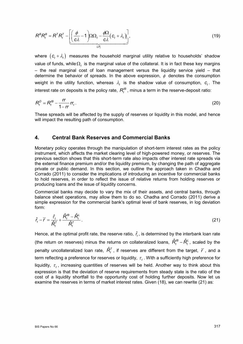
, (19)

where ( )λ+t tc measures the household marginal utility relative to households’ shadow

value of funds, whileΩt is the marginal value of the collateral. It is in fact these key margins – the real marginal cost of loan management versus the liquidity service yield – that determine the behavior of spreads. In the above expression, φ denotes the consumption weight in the utility function, whereas λt is the shadow value of consumption, tc . The

interest rate on deposits is the policy rate, IBtR , minus a term in the reserve-deposit ratio:

= −−1

D IBt t t

rrR R rrrr

. (20)

These spreads will be affected by the supply of reserves or liquidity in this model, and hence will impact the resulting path of consumption.

4. Central Bank Reserves and Commercial Banks

Monetary policy operates through the manipulation of short-term interest rates as the policy instrument, which affects the market clearing level of high-powered money, or reserves. The previous section shows that this short-term rate also impacts other interest rate spreads via the external finance premium and/or the liquidity premium, by changing the path of aggregate private or public demand. In this section, we outline the approach taken in Chadha and Corrado (2011) to consider the implications of introducing an incentive for commercial banks to hold reserves, in order to reflect the issue of relative returns from holding reserves or producing loans and the issue of liquidity concerns.

Commercial banks may decide to vary the mix of their assets, and central banks, through balance sheet operations, may allow them to do so. Chadha and Corrado (2011) derive a simple expression for the commercial bank's optimal level of bank reserves, in log deviation form:

τ −− = +

ˆ ˆˆˆˆ ˆ

IB Lt t t

t T Tt t

R Rr rR R

. (21)

Hence, at the optimal profit rate, the reserve ratio, tr , is determined by the interbank loan rate

(the return on reserves) minus the returns on collateralized loans, −ˆ ˆIB Lt tR R , scaled by the

penalty uncollateralized loan rate, ˆTtR , if reserves are different from the target, r , and a

term reflecting a preference for reserves or liquidity, τ t . With a sufficiently high preference for liquidity, τ t , increasing quantities of reserves will be held. Another way to think about this expression is that the deviation of reserve requirements from steady state is the ratio of the cost of a liquidity shortfall to the opportunity cost of holding further deposits. Now let us examine the reserves in terms of market interest rates. Given (18), we can rewrite (21) as:


τ

τ

−= + +

= − ++ +

ˆ ˆˆˆˆ ˆ

ˆ ,ˆ ˆ

IB Lt t t

t L Lt t

t tIB IBt t t t

R LRr rR R

EFP rR EFP R EFP

(22)

which introduces the trade-off between reserves being driven down (up) by a higher (lower) external finance premium, and the need to offset changes in the probability of a liquidity shortfall. We shall return to the policy implications of this result in the conclusion.

Figure 3 shows the effect of a liquidity preference for reserves on bank asset allocation across reserves and loans. Having produced a quantity of loans, tD , as a function of collateral and monitoring inputs, the banks lie on the line tangential between the production function and the allocation line. If there is a preference for liquidity over illiquidity, as necessitated by a financial intermediary that transforms maturity, reflecting inter alia the liquidity preference term, τ t , the bank will be better off if excess reserves can be supplied, and this will be accomplished by swapping loans for reserves at some rate of transformation which reflects the relative interest rates on the two activities. Now let us consider a simple thought experiment in which the rate of return on reserves increases and the return on loans stays constant. The allocation towards reserves per unit of loans will increase and reserves relative to loans will rise, and hence so will the reserve-deposit ratio. Similarly, if the rate of return on reserves falls, the rate of allocation to reserves will fall, and accordingly the reserve-deposit ratio will fall. For comparison, Figure 4 plots the ratio of the behaviour of reserves relative to loans for a fixed reserve-deposit ratio (black dotted line) and for changes induced by changes in the return on reserves alone (red line). The basic mechanism is illustrated here, but what we find in the model will result from the interaction of both loan rates and policy rates (which are paid on reserves), as well as the movement in the loan production function, and so we turn to the calibrated model.

5. Calibration

Table 2 provides a complete list of the endogenous and exogenous variables of the model and their meaning, while Table 3 reports the values for the parameters and Table 4 the steady-state values of the relevant variables.19 Following Goodfriend and McCallum (2007), we choose the consumption weight in utility,φ , to yield 1/3 of available time in either goods or banking services production. We also set the relative share of capital and labour in goods production η to be 0.36. We choose the elasticity of substitution of differentiated goods, θ , to be equal to 11. The discount factor, β , is set to 0.9, which is close to the canonical quarterly value, while the mark-up coefficient in the Phillips curve, κ , is set to 0.1. The depreciation rate, δ , is set to be equal to 0.025 while the trend growth rate, γ , is set to 0.005, which corresponds to 2% per year. The steady-state value of the bond holding level relative to GDP, b , is set to 0.56 as of the third quarter of 2005. The steady state of private sector bond

19 The equations for the steady-state equations are listed in Section A.4 of the technical appendix, available on

request.


holdings relative to GDP is set at 0.50, consistent with holdings of U.S. Treasury securities as of the end of 2006.20

The parameters linked to money and banking are defined as follows. Velocity at its steady-state level is set at 0.276, which is close to the ratio between U.S. GDP and M3 at fourth quarter 2005, yielding 0.31. The fractional reserve requirement, rr , is set at 0.1, which is higher than the value of 0.005 assumed by Goodfriend and McCallum (2007). The fraction of collateral, α , in loan production is set to 0.65 and the coefficient reflecting the inferiority of capital as collateral, k , is set to 0.2, while the loan production coefficient, F , is set to 9.14. The low value of capital productivity reflects the fact that banks usually use a higher fraction of monitoring services and rely less on capital as collateral.

With these parameter values we see that the steady state of labour input, n , is 0.31, which

is close to the required 1/3. The ratio of time working in the banking service sector, +

mm n

, is

1.9% under the benchmark calibration, not far the 1.6% share of total U.S. employment in depository credit intermediation as of August 2005. As the steady states are computed at zero inflation, we can interpret all the rates as real rates. The riskless rate, TR , is 6% per annum. The interbank rate, IBR , is 0.84% per annum, which is close to the 1% per year average short-term real rate. The government bond rate, BR , is 2.1% per annum. Finally, the collateralized external finance premium is 2% per annum, which is in line with the average spread of the prime rate over the federal funds rate in the U.S.21 The model is solved using the methods of King and Watson (1998), who also provide routines to derive the impulse responses of the endogenous variables to different shocks, to obtain asymptotic variance and covariances of the variables, and to simulate the data.22 For the impulse response analysis and simulation exercise we consider the real and financial shocks described in Table 5, which reports the volatility and persistence parameters chosen for the calibration and simulation exercise. These are standard parameters in the literature and simulate a fall in output consistent with the crisis.

6. Impulse Responses From Balance Sheet Policies

To understand the dynamics of this model, in this section we outline the impact of a negative shock to the value of collateral in the context of various adaptations of the original framework. Our financial sector shock operates through the asset price and can be thought of as a primitive representation of the shock which hit the U.S. housing market towards the end of 2007. This had a negative impact on the value of assets that households were able to post as collateral in exchange for loans in the form of housing. The securitisation of these mortgage loans, and their subsequent trade by financial intermediaries, meant that this also

20 The steady state of the transfer level, the Lagrangian of the production constraint and base money depend on

the above parameters. The steady state of the marginal cost is θθ−

=1mc .

21 The equations for the steady states are listed in the Technical Appendix. 22 The log-linearized equations for the model are listed in section C of the Technical Appendix. King and

Watson's MATLAB code is generalized, in that for any model we adapt three MATLAB files. The three files for the solution of our benchmark model, gmrsys.m, gmrdrv.m and gmrcon.m, are available on request. King and Watson's package includes standardized auxiliary programs, impkw.m, to generate the impulse responses to different shocks to the endogenous variables, as well as the program fdfkw.m to obtain the filtered autocovariances and the filtered second moments from the model solution. The program impkwsimu.m simulates the artificial series and makes it possible to generate HP-filtered data.


affected the value of collateral that banks themselves held, damaging their ability to raise funds.

We also analyse a case in which we negatively shock productivity in the manufacturing sector before briefly discussing the response of the system to a change in the composition of assets held on the central bank's balance sheet, in order to provide a simplistic insight into credit easing policies. Figures 5-9 plot the log deviation from steady-state responses of real consumption, inflation, the external finance premium, the liquidity premium, the policy rate, real deposits, real reserves, real loans, the reserve-deposit ratio, private sector bond holdings, the level of monitoring work employed, employment in the goods sector, asset prices, the bond rate and the loan rate.

6.1 The Role of Reserves We first show the mechanism through which reserve decisions can affect the real economy in our framework. Figure 5 shows the effects of our negative collateral shock under a regime of a fixed reserve-deposit ratio, compared to one in which reserves are decided endogenously by profit-maximising banks. In the first instance, when the shock hits there is an initial fall in asset prices, which reduces the efficiency of producing loans, as households have less collateral to post. As bonds are fixed, producing the same amount of loans would require an increase in monitoring effort on the part of the banks, and thus make loan production more expensive. This causes the external finance premium to increase, and through the cash-in-advance constraint we see a fall in consumption and deposits, which increases the EFP yet further. Since the reserve/deposit ratio is fixed, the fall in deposits leads to a proportional fall in loans and reserves. In response to the fall in output and inflation, the central bank cuts the policy rate and the economy returns to equilibrium.

Alternatively, if the reserve decision is endogenised and the reserve-deposit ratio is allowed to fluctuate, then as the cost of providing loans increases, banks demand more reserves and the central bank supplies them perfectly elastically. This allows banks to shed the now more costly loans, pushing up the reserve-deposit ratio, which means that the EFP rises less, with monitoring effort actually falling and with a smaller contraction in consumption. The smaller decline in consumption is mirrored by a smaller decline in deposits, and the policy rate now follows a much smoother path as reserve policy takes some of the burden of stabilising the economy. Thus, we can see that reserves have a significant role to play in our economy due to their financial attenuation effects.

In the recent crisis, policymakers were faced with having to respond to a contractionary shock, whilst their default policy tool, the short-term nominal interest rate, was constrained by the zero lower bound. To investigate this in the context of our model we deactivate the Taylor rule, holding the policy rate constant, and subject the model to the same negative collateral shock. What we see in Figure 5 is that because the policy rate does not fall in response to the downturn in consumption and inflation, the return from holding reserves is even higher, increasing the level of demand from financial intermediaries. This creates an even larger response in reserves than we saw under an active interest rate policy, which attenuates the rise in the external finance premium to such an extent that it temporarily falls before returning to equilibrium. The strength of this attenuation is enough to bring consumption and inflation back to equilibrium along more or less the same path as when interest rate policy was unconstrained. This suggests that altering the level of reserves on commercial banks' balance sheets can stabilise the economy, even in the absence of interest rate policy.

6.2 Open Market Operations In practice, changes in the level of reserves are effected via open market operations. The central bank buys (sells) assets from the private sector in exchange for an increased (decreased) level of reserves. Recent quantitative easing policies are theoretically just extensions of these operations, differing only in their unprecedented magnitude.


In order to realistically model OMOs, we must augment the original endogenous reserves framework to take account of this swap of reserves for assets. Reserves, which are the central bank's only liability, must be backed by equally valued asset holdings. Initially, we assume the central bank holds only government bonds, the total supply of which is fixed unless exogenously shocked. This means that in order to increase the level of reserves, the central bank must buy bonds from the private sector, increasing the fraction of total bonds it holds, and decreasing the amount held by the private sector.

To model this, we define total bond holdings as the sum of private sector and central bank bond holdings:

= +CB Pt t tb b b , (23)

and as central bank bond holdings must equal reserves, we can substitute and rearrange to give the log linear relationship

= −ˆ ˆ ˆp pt t t t t tb b b b r r , (24)

which we add to our system of equations. It is this newly defined variable pb which determines the amount of collateral that households have available, so we substitute it for b in the equations for loan supply and marginal value of collateralized lending.23

An alternative is to swap the other type of asset in our economy, capital. This is less liquid and less efficient as collateral, but could be bought by the central bank in exchange for new reserves in the same way that bonds are. For this operation, we introduce an equation defining total capital holdings as a function of an exogenous shock, in the same way as we did for bond holdings. The central bank can now hold two assets on its balance sheet, so we hold the level of bonds fixed, as before, and set the steady-state value of capital held by the central bank at zero. By defining private sector capital holdings in a log linear form as

= −ˆ ˆ ˆp pt t tk k bb rr , (25)

what we model is a situation where the central bank buys and sells illiquid assets/capital in exchange for reserves.

In Figure 6 we can see how a negative collateral shock propagates in the presence of each type of OMO when the short-term nominal interest rate is constrained. It appears that the type of asset exchanged has very little impact on the path taken by key variables or on the mechanism through which the policy works. This poses no deep problem in itself, as one of the core motivations for making these adaptations to the model is to ensure that the policy we model can be related as closely as possible to the practical conduct of real world policies. However, during our welfare analysis in the following section we see that there are differences between the implications of differing styles of OMOs. This suggests a channel by which OMOs such as those carried out by central banks post-crisis can be an effective and practical means to stabilise the economy, even in the absence of an active interest rate policy.

23 As we deal with a consolidated government budget constraint, the net effect of interest payments on bonds

held by the central bank is zero. Therefore, it is appropriate to change the terms in b to terms in pb in this equation as well.


6.3 The Role of Policymakers Having demonstrated a clear role for reserves in this model, the next question is how to control this policy tool. If the central bank chooses to supply reserves perfectly elastically to meet the demand of the banking sector, then banks will set that demand at the level which is optimal for them in terms of profits. This can be thought of as a financially optimal path for reserves. It may not, however, be consistent with the macroeconomic optimum desirable to policymakers. To test this, we compare the model where reserves are determined by the banking sector's demand to one where the central bank determines reserve levels in response to a simple policy rule dependent on inflation:

( ) πρ φ π ρ −= − + 1ˆ ˆ1 ˆt r t r tr r (26)

Figure 7 shows that in response to a negative collateral shock, as far as stabilising key macroeconomic variables is concerned, even an incredibly simple policy rule can outperform the situation where bank set the level of reserves. This is because the central bank is at first more aggressive, forcing the financial intermediaries to take on more reserves than would be profit-maximising for them, and this provides a greater attenuation of the EFP via the same mechanisms that an increase in reserves works through when chosen by banks. This brings the economy back to equilibrium more quickly, and the level of reserves returns more quickly to its steady state.

The key point to be taken from Figure 7 is that the financially optimum path for reserves and the macro-optimal path are not always the same, suggesting an important role for policymakers in monitoring and setting the reserve levels of financial institutions, which have an incentive to try and keep reserve levels away from the macro optimal level.

This result holds true when we constrain the policy rate, and also when we vary which of the exogenous shocks we put through the system, with one exception: a productivity shock. Figure 8 shows that if our contraction is caused by an exogenous fall in productivity in the manufacturing sector, then our policy rule causes a deeper and more prolonged fall in real consumption/output. This is due to the fact that under a productivity shock, inflation and output move in opposite directions, causing a conflict of objectives for the central bank. As the central bank follows its policy rule and cuts reserves to curb the higher inflation, this simultaneously induces a fall in consumption, worsening the contraction already experienced.

6.4 The Implications of Balance Sheet Composition So far we have considered policies which can be loosely termed quantitative easing, where reserve levels, and thus the size of the central bank's balance sheet, are allowed to fluctuate. In practise, however, many central banks carried out at least a degree of credit easing (CE) alongside their quantitative easing programmes, especially in the U.S. CE differs from QE in that the overall level of reserves doesn't need to change, but the central bank changes the mix of assets on its balance sheet, buying up less liquid assets and selling off more liquid ones, to increase liquidity to the private sector. Eggerston and Woodford (2003), among others suggest that this should have no impact on the wider economy, as there is no reason for it to change agents' long-term expectations regarding monetary policy.

In the context of our model, with reserves determined by commercial banks' demand, we can outline a very basic credit easing policy by simulating a swap, exogenously increasing the level of liquid bonds held by the private sector and simultaneously reducing the level of less liquid capital. When we run this credit easing swap (Figure 9), what we find is that the marginal value of collateralized lending decreases since there are more liquid assets available to be put up as collateral by the private sector, increasing the efficiency of loan production. This causes consumption to rise and the level of monitoring effort needed by banks to fall, both of which decrease the EFP. The liquidity premium drops as consumption rises and the marginal value of collateralized lending falls, whilst the central bank raises the


policy rate in response to the increase in inflation and output. The improved economic conditions subsequently lead to an increase in reserves, but one that is less than the increase in lending. This result implies that if credit easing were employed countercyclically, it would be a useful tool in limiting rises in the EFP and liquidity premium, such as those much of the world has experienced recently, even if the policy rate is constrained by increasing the quantity of more liquid assets available to be used by banks as collateral for loans, thus increasing their loan production efficiency.

6.5 Welfare Analysis Table 6a shows the asymptotic standard deviation and the contemporaneous cross-correlation with consumption from a simulation of the model, allowing us to compare a fixed reserve-deposit ratio regime with one in which reserves are determined by commercial banks and one in which they are set by a central bank policy rule. We also show the results for each type of reserve setting policy with the policy rate constrained, so as to highlight the efficacy of policies should the policymakers find themselves unable to use interest rate policy.

What we find is that endogenising reserves can dramatically lower the standard deviation of inflation, asset prices and the policy rate, but at the expense of increased standard deviation in output and monitoring work. There is also an increased deviation in the external finance and liquidity premia. Perhaps counterintuitively, the standard deviation of reserves falls. This is due to the fact that under a ‘fixed’ regime, reserves have to constantly move in order to maintain a constant reserve-deposit ratio, whilst in a scenario of endogenous reserve setting this is smoothed. By introducing a reserve policy rule we manage to reduce the standard deviation in inflation and asset prices even further, but manage to negate some of the trade-off with monitoring work, the EFP and liquidity premium, and especially consumption, which has a lower standard deviation under a reserves rule than under a fixed reserve-deposit ratio. It is worth noting that when the nominal interest rate is constrained, there is an increase in the standard deviation of output, inflation asset prices and other variables, but in an almost equal amount regardless of which of the two policy rules is implemented.

Table 6b shows the same information for models in which open market operations are present, responding to endogenous, bank-determined reserve levels. We see here that conducting OMOs by swapping reserves for bonds results in much lower standard deviations, in all but one variable, than occurs when the OMOs are conducted through swaps for capital, even when the interest rate is constrained. The standard deviation of private sector bond holdings logically increases since bonds are now part of an active policy tool. Figure 10 shows the middle segment, as an illustration, from a simulation of 10,000 data points (with the first 500 observations discarded) of key macroeconomic variables under each policy regime. The simulated data are HP-filtered ( )λ = 1600 . Plotting the reserve-deposit ratio we see that endogenising reserves causes the reserve-deposit ratio to fluctuate as it responds to commercial bank demand. These fluctuations can be smoothed, and a degree of volatility removed, by the central bank’s taking control of reserve policy with an active reserves rule.

6.5.1 Approximating the welfare function The welfare approximation derived from the canonical New Keynesian model finds that welfare of the representative household only depends on the variance of output and inflation (Galí, 2008). We wish to investigate whether this result continues to hold when applied to our richer class of model. The use of the approximation allows us to quantify precisely the welfare rankings arising from each of our policy rules, possibly allowing some normative


statements. Thus, we derive a quadratic loss function using a second-order Taylor approximation to utility by using the labour demand function, marginal cost function and sales production constraint to substitute for household consumption.24 Once this is reordered and simplified, we are left with a loss function with relevant terms in the variances of consumption, inflation, wages, employment in the goods sector and marginal cost.25

( ) ( )

( )( )( )

π

β

θσ η ση

σ σ σ

θ βθ ηθ η θ

∞

=

− = − +

+ + − + Χ − = − + − − −

Χ =+ −

∑00

2 2 2

2 2 2

with

where

1 32

11 12

1 1 1 .1 1

tt t

t

c

t

w n mc

U U E L O

w nc cL

w n mcc c c

(27)

Remark: The welfare of the representative household in this model, as in the original New Keynesian framework, is approximated by standard variables on the supply side rather than those specifically attributable to financial factors. This means that changes in financial conditions do not directly impact utility, but only impact the variance of consumption, inflation, wages, labour supply hours and marginal costs.

Having obtained the welfare approximations, we can calculate the loss under each policy rule at the benchmark calibration and then rank the losses using the metric laid out by Gilchrist and Saito (2006), which is defined as the ratio between the loss obtained from implementing a given policy rule χ versus a benchmark policy rule, and the loss obtained under the most stabilising policy rule versus the same benchmark.

( ) ( ) ( )( ) ( )

χχ

−=

−Benchmark Policy Policy

Benchmark Policy Most StabilisingL L

GainL L

(28)

If this relative gain criterion is less (more) than one, then the given policy can be said to be worse (better) than the most stabilising policy. If it is negative, then the given policy actually performs worse than the benchmark. This metric allows us to explicitly rank our policies. For our calculations we chose an active interest rate policy rule under a fixed reserves system as our benchmark, and our most stabilising reference policy is an active interest rate policy alongside a central bank reserve rule responding to inflation. Table 7 confirms that whilst all endogenous reserve policies outperform a fixed reserve system, our best welfare outcome is reached by allowing the central bank to control both the policy rate and the reserve level in response to macroeconomic factors. Within this framework, OMOs conducted by swapping reserves for bonds have better welfare implications than OMOs carried out via a swap for capital, but they only marginally outperform our benchmark endogenous reserves model. An interesting aspect of this analysis is that we can see the relative loss in welfare caused by the short-term nominal interest rate’s becoming constrained (CIR), by comparing an endogenous reserves system that incorporates interest rate policy with one of just

24 The additive nature of our household's utility function allows us to take a Taylor expansion of each term and

substitute it back into the original function. The labour demand function is then rearranged for monitoring work, a second-order expansion taken and a substitution made. This process is then repeated for the marginal cost equation. Following Galí (2008), we substitute the resulting linear term in goods sector employment for a second-order term in inflation, using the sales equal to net production constraint.

25 The welfare approximation is derived in Section F of the Technical Appendix.


endogenous reserves. The size of the loss suggests that when confronted with the ZLB, policymakers operating an active reserve strategy may be able to limit welfare losses despite not being able to use their major policy tool.

The supply of liquidity through the issuance of reserves alongside an active interest rate would appear to reduce the welfare losses faced by the representative household over the business cycle. Reserves attenuate the fluctuations in the external finance premium in response to demand (consumption) and supply (loans) responses to shocks. A banking sector with a liquidity preference is better off when liquidity is supplied over the business cycle, and because the requirement for loans from the private sector can in part be met by increasing reserves rather than by increasing costly monitoring. Reserves as a monetary/fiscal instrument allow the banks to hedge liquidity risk and also improve macroeconomic outcomes, so there is not necessarily a trade-off between financial and monetary stability.

6.6 Balance Sheet Policy and the Business Cycle Table 8 shows the asymptotic standard deviation and contemporaneous cross-correlation with real consumption (output) of the reserve-deposit ratio and nominal spending under each policy regime. What we see is that, as with consumption, inflation and asset prices, we can lower the standard deviation on nominal spending by endogenising our reserve decision, and still further if we allow reserves to be set by a policy rule. The fixed nature of the reserve-deposit ratio in the first regime means that by design we have zero standard deviation, but as we allow it to fluctuate and take on an active role as a policy tool, our reserves rule, which gives the best welfare option, actually has the lowest standard deviation.

To contextualize these movements in terms of the business cycle, we can analyse how the movements of these variables are correlated with real GDP, or in the case of our model, consumption. Endogenising the reserves decision creates a deal of procyclicality in the reserve-deposit ratio, suggesting that in a boom period commercial banks build up their stock of reserves relative to loans and then run them down in an economic downturn. This is a key part of the mechanism by which the financial attenuator works as a systematic policy tool. Under a reserve rule this procyclicality is mostly removed, as reserves react to inflation, not output. Nominal spending also becomes more procyclical as we endogenise reserves, since we dampen fluctuations in the price level, bringing real consumption and nominal spending much closer together.

7. Conclusions

This paper uses a micro-founded macroeconomic model to consider the implications of balance sheet, or non-conventional, monetary policies in which bank lending, interest rate spreads and the variance of the central bank balance sheet are shown to matter. To the model of Goodfriend and McCallum (2007) we append velocity shocks in the demand for money function (see Chadha, Corrado and Holly, 2008) as well as a process for commercial bank reserve accumulation (see Chadha and Corrado, 2011), and then show that these policies can map onto central bank balance sheet policies. The issuance of reserves swaps short-term debt obligations for long-term obligations and thus improves the liquidity of the banking sector. The converse is also true. We then find that varying the central bank balance sheet attenuates the excessive volatility in the external finance premium that would otherwise ensue. We also solve for commercial banks' optimal levels of illiquid (loan) and liquid (reserves) asset holdings, and for the government's budget position, by allowing two forms of debt liabilities to be issued: one-period debt to finance any excess in government expenditures over tax receipts, and debt to finance the issuance of reserves. We are then able to consider the implication of one-off balance sheet operations as well as systematic adoption of balance sheet policies.


We find that balance sheet policies can also contribute to the stabilisation of the economy when the interest rate rule is constrained. Our impulse responses show that policies that expand the central bank balance sheet can stabilise the economy. Rules that swap reserves for assets perform well compared to a straight injection of reserves. We also examine the welfare implications of balance sheet policies and find that when reserves are set countercyclically – ie expanding when the economy contracts – then, generally speaking, the welfare of the representative household is better than under an active interest rate rule alone. This is because by setting both the quantity and price of central bank money the central bank can amplify control of a monetary economy. Rather than just setting interest rates and letting the money supply be elastically shaped by demand, some extra incentives are placed on financial activity to prevent the exacerbation of the cycle (Walsh, 2009). Encouraging the central bank to alter the size of its balance sheet will not only increase the efficacy of standard interest rate policy but also help prevent excesses of financial intermediation. However, ultimately these operations are fiscal and require the debt authority to accept the responsibility of hedging liquidity shortages or gluts in the financial sector.


Table 1

Consolidated Federal Reserve Balance Sheet Pre- and Post-Crisis

Assets Value (Millions of Dollars)

December 2007 July 2011

Gold Certificate Account 11,037 11,037 Special Drawing Rights Certificates Account 2,200 5,200 Coin 1,017 2,096 Securities, Repurchase Agreements and Loans 815,979 2,660,990 Securities Held Outright 779,640 2,648,438 U.S. Treasury Securities 779,640 1,624,515 Bills 267,019 18,423 Notes & Bonds1 512,621 1,606,092 Federal Agency Debt Securities – 115,070 Mortgage Backed Securities – 908,853 Repurchase Agreements 35,000 0 Loans 1,338 12,552 Net Portfolio Holdings Maiden Lane I, II & III – 59,637 Net Portfolio Holdings TALF LLC – 757 Items in Process of Collection 7,235 419 Bank Premises 2,079 2,199 Other 37,244 131,714 Total2 876,791 2,874,049

Liabilities FR Notes (Net of FR Bank Holdings) 778,611 990,861 Reverse Repo Agreements 35,098 67,527 Deposits 16,112 1,741,336 Held by Deposit Institutions 11,286 1,663,022 U.S. Treasury Account, General 4,489 67,270 U.S. Treasury Supplementary Financing Account – 5,000 Foreign Official 97 127 Other 241 5,918 Deferred Availability Cash Items 6,509 2,074 Other Liabilities and Accrued Dividends 6,066 20,584 Capital Accounts 34,345 51,667 Total 876,791 2,874,049 1 Includes nominal, inflation-indexed and inflation-compensated. 2 Preferred interests in AIA Aurora LLC and ALICO Holdings LLC do not appear, as they were repaid as of January 2011. Likewise, CPFF has been fully repaid and no longer appears.


Table 2

The Variables

Variable Description

c Real Consumption

n Labour Input

m Labour Input for Loan Monitoring, or 'Banking Employment'

w Real wage q Price of Capital Goods

P Price Level

π Inflation

mc Marginal Cost

r Reserves

rr Reserves/Deposit Ratio

D Deposits

L Loans AP Aggregate Prices

b Real Bond Holding pb Real Private Sector Bond Holdings

Ω Marginal Value of Collateral

EFP Uncollateralized External Finance Premium ( )T IBR R−

BLSY Liquidity Service on Bonds

KBLSY Liquidity Service on Capital ( )BkLSY

TR Benchmark Risk Free Rate BR Interest Rate for Bond IBR Interbank Rate LR Loan Rate DR Deposit Rate

λ Lagrangian for Budget Constraint (shadow value of consumption)

ξ Lagrangian for Production Constraint

T Real transfer (%)


Table 3

Parameterisation

Parameter Description Value

β Discount factor 0.9

κ Coefficient in Phillips curve 0.1 α Collateral share of loan production 0.65 φ Consumption weight in utility 0.4 η Capital share of firm production 0.36 δ Depreciation rate of capital 0.025 γ Trend growth rate 0.005 ρ Interest rate smoothing 0.8

πφ Coefficient on Inflation in Policy 1.5

yφ Coefficient on Output in Policy 0.5

F Production coefficient of loan 9.14 k Inferiority coefficient of capital as collateral 0.2 θ Elasticity of substitution of differentiated goods 11


Table 4

Steady States

Steady State Description Value

m Banking Employment 0.0063

n Labour Input 0.3195 TR Risk Free Rate 0.015

IBR Interbank Rate 0.0021

LR Loan Rate 0.0066

LR Bond Rate 0.0052

b c Bond to Consumption Ratio 0.56

pb c Private Sector Bond Holdings to Consumption Ratio 0.50

c Consumption 0.8409

T c Transfers over consumption 0.126

w Real Wage 1.9494

λ Shadow Value of Consumption 0.457

v Velocity 0.31

Ω Marginal Value of Collateral 0.237

K Capital 9.19 PK Private Sector Capital Holdings 9.19

rr Reserve ratio 0.1

r c Reserves to Consumption 0.36

Table 5

Properties of Exogenous Shocks

Shock Name Standard Deviation Persistence

Productivity 0.35% 0.95

Monitoring 1.00% 0.95

Collateral 0.35% 0.9

Monetary Policy 0.82% 0.3

Mark Up 0.11% 0.74

Bond Holdings 1.00% 0.9

Velocity 1.00% 0.33

Liquidity 1.00% 0.33

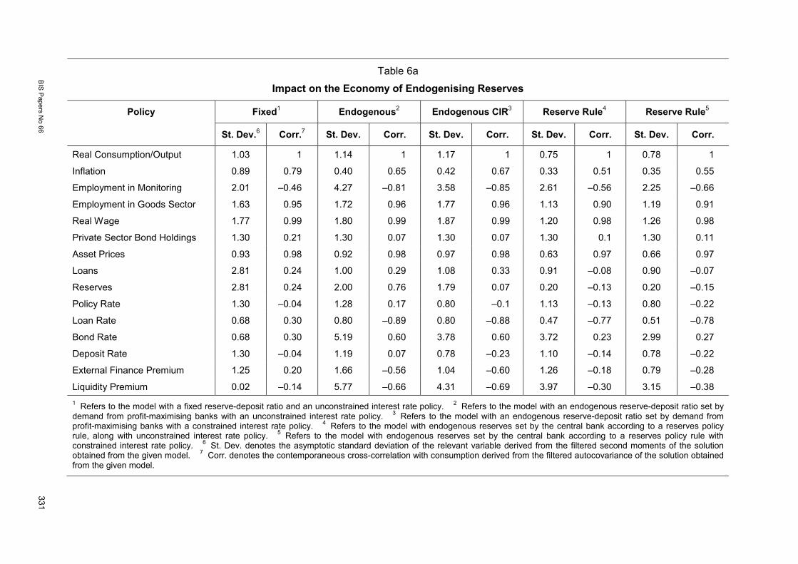
BIS

Papers N

o 66 331

Table 6a

Impact on the Economy of Endogenising Reserves

Policy Fixed1 Endogenous2 Endogenous CIR3 Reserve Rule4 Reserve Rule5

St. Dev.6 Corr.7 St. Dev. Corr. St. Dev. Corr. St. Dev. Corr. St. Dev. Corr.

Real Consumption/Output 1.03 1 1.14 1 1.17 1 0.75 1 0.78 1

Inflation 0.89 0.79 0.40 0.65 0.42 0.67 0.33 0.51 0.35 0.55

Employment in Monitoring 2.01 –0.46 4.27 –0.81 3.58 –0.85 2.61 –0.56 2.25 –0.66

Employment in Goods Sector 1.63 0.95 1.72 0.96 1.77 0.96 1.13 0.90 1.19 0.91

Real Wage 1.77 0.99 1.80 0.99 1.87 0.99 1.20 0.98 1.26 0.98

Private Sector Bond Holdings 1.30 0.21 1.30 0.07 1.30 0.07 1.30 0.1 1.30 0.11

Asset Prices 0.93 0.98 0.92 0.98 0.97 0.98 0.63 0.97 0.66 0.97

Loans 2.81 0.24 1.00 0.29 1.08 0.33 0.91 –0.08 0.90 –0.07

Reserves 2.81 0.24 2.00 0.76 1.79 0.07 0.20 –0.13 0.20 –0.15

Policy Rate 1.30 –0.04 1.28 0.17 0.80 –0.1 1.13 –0.13 0.80 –0.22

Loan Rate 0.68 0.30 0.80 –0.89 0.80 –0.88 0.47 –0.77 0.51 –0.78

Bond Rate 0.68 0.30 5.19 0.60 3.78 0.60 3.72 0.23 2.99 0.27

Deposit Rate 1.30 –0.04 1.19 0.07 0.78 –0.23 1.10 –0.14 0.78 –0.22

External Finance Premium 1.25 0.20 1.66 –0.56 1.04 –0.60 1.26 –0.18 0.79 –0.28

Liquidity Premium 0.02 –0.14 5.77 –0.66 4.31 –0.69 3.97 –0.30 3.15 –0.38 1 Refers to the model with a fixed reserve-deposit ratio and an unconstrained interest rate policy. 2 Refers to the model with an endogenous reserve-deposit ratio set by demand from profit-maximising banks with an unconstrained interest rate policy. 3 Refers to the model with an endogenous reserve-deposit ratio set by demand from profit-maximising banks with a constrained interest rate policy. 4 Refers to the model with endogenous reserves set by the central bank according to a reserves policy rule, along with unconstrained interest rate policy. 5 Refers to the model with endogenous reserves set by the central bank according to a reserves policy rule with constrained interest rate policy. 6 St. Dev. denotes the asymptotic standard deviation of the relevant variable derived from the filtered second moments of the solution obtained from the given model. 7 Corr. denotes the contemporaneous cross-correlation with consumption derived from the filtered autocovariance of the solution obtained from the given model.

332 B

IS P

apers No 66

Table 6b

The Impact on the Economy of Different Methods of Conducting Open Market Operations

Policy Bond OMO1 Bond OMO CIR2 Capital OMO3 Capital OMO CIR4

St. Dev. Corr. St. Dev. Corr. St. Dev. Corr. St. Dev. Corr.

Real Consumption/Output 1.03 1 1.07 1 1.21 1 1.24 1

Inflation 0.39 0.61 0.41 0.64 0.50 0.70 0.54 0.72

Employment in Monitoring 4.08 –0.77 3.44 –0.82 4.25 –0.73 3.69 –0.68

Employment in Goods Sector 1.56 0.95 1.62 0.95 1.83 0.96 1.89 0.96

Real Wage 1.62 0.99 1.70 0.99 1.94 0.99 2.03 0.99

Private Sector Bond Holdings 1.83 –0.35 1.79 –0.32 1.30 0.33 1.30 0.33

Private Sector Capital Holdings – – – – 1.30 0.30 1.31 0.30

Asset Prices 0.84 0.98 0.88 0.98 1.00 0.98 1.05 0.99

Loans 0.96 0.16 1.03 0.21 1.52 0.34 1.66 0.36

Reserves 1.83 0.70 1.64 0.71 1.97 0.68 1.78 0.65

Policy Rate 1.24 0.11 0.80 –0.12 1.35 0.22 0.80 –0.09

Loan Rate 0.71 –0.87 0.71 –0.86 0.78 –0.76 0.79 –0.73

Bond Rate 4.90 0.54 3.63 0.54 5.38 0.62 3.80 0.59

Deposit Rate 1.16 0.03 0.78 –0.25 1.30 0.16 0.80 –0.16

External Finance Premium 1.55 –0.49 0.96 –0.53 1.68 –0.53 1.03 –0.49

Liquidity Premium 5.39 –0.61 4.07 –0.63 5.89 –0.67 4.28 –0.65 1 Refers to the model in which OMOs are carried out via an exchange of reserves for bonds to meet endogenous reserve demand of banks, along with unconstrained interest rate policy. 2 Refers to the model in which OMOs are carried out via an exchange of reserves for bonds to meet endogenous reserve demand of banks with constrained interest rate policy. 3 Refers to the model in which OMOs are carried out via an exchange of reserves for capital to meet endogenous reserve demand of banks, along with unconstrained interest rate policy. 4 Refers to the model in which OMOs are carried out via an exchange of reserves for capital to meet endogenous reserve demand of banks with constrained interest rate policy.


Table 7

Relative Welfare Analysis

Policy Regime Welfare Loss Gain Criterion

Fixed 24.21 0

Endogenous 10.48 0.73

Endogenous CIR 11.38 0.69

Reserve Rule 5.53 1

Reserve Rule CIR 6.14 0.97

Bond OMO 9.01 0.81

Bond OMO CIR 9.94 0.76

Capital OMO 13.57 0.57

Capital OMO CIR 15.24 0.48


Table 8

Balance Sheet Policies and the Business Cycle1

Reserve-Deposit Ratio Nominal Spending

Fixed

St. Dev. 0 2.84

Corr. 0 0.40

Endogenous

St. Dev. 1.70 1.51

Corr. 0.65 0.82

Endogenous CIR

St. Dev. 1.52 1.58

Corr. 0.61 0.81

Reserves Rule

St. Dev. 0.93 1.03

Corr. 0.05 0.68

Reserves Rule CIR

St. Dev. 0.94 1.08

Corr. 0.03 0.67

Bond OMO

St. Dev. 1.72 1.39

Corr. 0.59 0.78

Bond OMO CIR

St. Dev. 1.54 1.47

Corr. 0.56 0.78

Capital OMO

St. Dev. 1.94 1.82

Corr. 0.38 0.75

Capital OMO CIR

St. Dev. 1.96 1.92

Corr. 0.25 0.73 1 Corr. denotes the contemporaneous cross-correlation of the given variable with real consumption/output.


Figure 1

Federal reserve assets1

1 Total may differ from constituent parts, due to rounding.

Figure 2

Federal reserve liabilities

0

0.5

1

1.5

2

2.5

3

Sep 2007 Sep 2008 Sep 2009 Sep 2010

Securities Held Outright Term Auction Credit Commercial Paper Funding Facility

Central Bank Liquidity Swaps Term Asset-Backed Securities Loan Facility Support for Specific Institutions

Total Assets

USD (Trillions)

0

0.5

1

1.5

2

2.5

3

Sep 2007 Sep 2008 Sep 2009 Sep 2010

USD (Trillions)

Currency in Circulation Reserves Supplementary Treasury Financing Account Total Liabilities


Figure 3

Production of loans and liquidity preference of banks

Figure 4

Reserves over the business cycle

BIS

Papers N

o 66 337

Figure 5

Response to negative 1 standard deviation shock to the value of collateral under fixed and endogenous reserve-deposit ratios and with the nominal interest rate constrained

338

BIS

Papers N

o 66

Figure 6

Response to negative 1 standard deviation shock to the value of collateral under different styles of OMO with a constrained short-term nominal interest rate

BIS

Papers N

o 66 339

Figure 7

Response to negative 1 standard deviation shock to collateral under different reserve setting regimes

340

BIS

Papers N

o 66

Figure 8

Response to negative 1 standard deviation shock to productivity in manufacturing under different reserve setting regimes

BIS

Papers N

o 66 341

Figure 9

Response to a primitive credit easing policy controlled by equal and inverse exogenous shocks to private sector bond holdings and private sector capital holdings


Figure 10

Simulation of two-year moving average series of HP-filtered reserve-deposit ratio under three reserve regimes1

1 Figure 10 shows the middle segment of a simulation of 10,000 data points based on each reserve setting model. The simulated data are HP-filtered (λ =1600).


Technical Appendix

A. Model Setup

This is a modified version of the Goodfriend and McCallum (2007) model, incorporating a government (including bank) budget constraint and a cash-in-advance constraint with stochastic velocity of money demand from Chadha and Corrado (2011).

• Utility function:

( ) ( ) ( )00

log 1 log 1t s st t t

tU E c n mβ φ φ

∞

=

= + − − − ∑, (29)

where tc denotes real consumption, stn is supply of labour in goods sector and s

tm is the supply of monitoring work in the banking sector.

• Budget constraint:

( ) ( )

( ) ( )

1

1

11

1

1

s s At t tt t t t t t tA A A

t t t

t tt t t t t t tA A B

t t t

B D Pq K w n m c

P P PD B

w n m tax q K cP P R

θγ

δ

γ

−

−

++

− + + + + + + Π

− + − − − − −+

,

(30)

where tq is the price of capital, tK is the quantity of capital, tP is the price of household's produced good, A

tP is the consumption goods price index, tn is the labour demanded by household as producer, tm is the labour demanded by household's banking operation, tw is the real wage, tD is the nominal holding of broad money, ttax is the real lump-sum tax payment, B

tR is the nominal interest rate on government bonds purchased in 11, tt B ++ . We also assume that any profit from the banking sector, tΠ , goes to the household sector. The Lagrangian multiplier of this constraint is denoted as tλ .

• Sales equal net production constraint:

( ) ( )11 0A At t t t t tK A n c P P

θηη −−− = . (31)

1tA is a productivity shock in the goods production sector whose mean increases over time at a rate γ . In (18) and (19) the superscript A indicates that the variable is an aggregate taken as given from each household. The Lagrangian multiplier of this constraint is denoted as, tξ .

• Government (including bank budget constraint):

( ) ( )1 1

11 1t t t t

t t A AA IB A Bt tt t t t

r r B Bg tax

P PP R P Rγ γ− +

+

− = − + −+ +

, (32)

where tg is real government expenditure. We define:


( )( )

1 1 11

1

A Bt t t t

A IBt t t t

b B P R

re r P R

+ + += +

= +.

(33)

So the budget constraint can be rewritten as:

( ) ( )1 11 1 11 1

A AIB Bt t

t t t t t t tA At t

P PT re re R b b R

P P− −

− − −= − + + − +, (34)

where t t tT g tax= .

• Deposit/money constraint: A

t t t tc v D P= , (35)

where tv denotes velocity and tD are deposits.

• Loans:

( )1t t tL D rr= − , (36)

where tt

t

rrr

D= is the reserve-deposit ratio and tt is high-powered money.

• The bank's problem (see Baltensperger, 1980) is to maximize intra-period profits subject to the returns from loans, tL , which are lent out at the collateralized interest rate of LR , to the returns from reserves held at the central bank, tR , which are assumed to pay the interbank (policy) interest rate, IBR , and the payment of deposit interest, DR , to deposits:

max ,t

L IB Dt t t t t t t

rR L R r R DΠ = + − (37)

( ) ( )21s.t.2

Tt t t t tC R r r r rτ= − + − . (38)

Production function pertaining to management of loans:

( ) ( )1 13 2 1 0 1At t t t t t t tL P F b A kq K A mαγ α α+ += + − < < . (39)

From (35):

( ) ( )( )

11 13 2

1t t t t t t

t t At t

F b A kq K A mc v

P rr

α αγ −+ ++

=− ,

(40)

where 2tA denotes a shock to monitoring work, and 3tA is a shock to capital as collateral. The parameter k denotes the inferiority of capital as collateral in the banking production function, while α is the share of collateral in the loan production function. For a complete list of all variables and parameters in the model, see Tables 1 and 2 in the main text.

A.1 First-order conditions

• Derivative with respect to stm and s

tn of (29) and (30):


( )10

1 t ts st t

wn m

φλ

−− + =

− − (41)

• Derivative with respect to tm :

0

1

t tt t t

t t t

tt

t t t

c cw

c m m

cw

c m

φ λ λ

φλ

∂ ∂− − =

∂ ∂

∂= − ∂ ,

(42)

given that

( )( ) ( )

( )

11 13 2

11t t t t t t tt t t t

t A Att t t

v F b A kq K A mv D v Lc

rrP P rr

α αγ −+ ++

= = =−− .

(43)

Then

1tt

t t

cc

m mα∂ −

=∂ ,

so (42) becomes:

11t tt t t

w cc mφ αλ

−= − .

(44)

• Derivative with respect to tn :

( )

( )

1 11

1 11

tt t t t

t t

t tt t

t t t

Kw A

n A

Kw A

n A

η

η

λ ξ η

ξη

λ

= −

= −

.

(45)

• Derivative with respect to 1tK + :

( ) ( )111 1

1 1

1 1t tt t t t t t t t t t t

t t t

c cE q q E K A n

c K Kηηφ λ δ β λ λ ξ βη −−

+ ++ +

∂ ∂+ − − − +

∂ ∂ (46)

given

1 1 1

33

3

t t t t

t t t t t

t t t

c c A kqK b A kq K

A k

αγ+ + +

∂=

∂ +

= Ω (47)

with

1 13t

tt t t t

cb A kq K

αγ + +

Ω =+ .

(48)

So

( )1

1 1 11

1

11 3 1t t t t tt t t t t t

t t t t t t

A nA kq E q q E

c K

ηλ λ ξφ δ β βη

λ λ λ λ

−

+ + ++

+

− Ω + − − + .

(49)


• Derivative with respect to tP :

( ) ( ) ( ) ( ) ( ) ( )1 10 1 A A A At t t t t t t tc P P c P P

θ θθ θλ θ θξ− −− − −

= − + (50)

1t tA

t t

PP

ξ θλ θ

−=

.

• Derivative with respect to 1tB + :

( )1

1 1 1 1

01

t t t tt t A A B

t t t t t t

c cE

c B B P P Rλ γλφ λ βγ +

+ + + +

∂ ∂− + − =

∂ ∂ +,

where

( )1 1t t

A Bt t t

cB P R

γ

+

∂ Ω=

∂ +.

So

( ) ( )

( )

1

1

1

1

11 1

1 1 1

t t tt AA B A B

t t tt t t t

ABt t

t t tAt t t t

Ec PP R P R

PE R

c P

γ λ γλφ γβλ

λφ βλ λ

+

+

+

+

Ω= − + −

+ +

= − Ω − + + .

(51)

• Derivative wrt tr of (37) and (38):

( ) 0L IB Ttt t t t t

t

R R R r rr

τδ∂Π

= − + − − − = . (52)

IB Lt t t

t Tt

R Rr r

Rτ + −

= +. (53)

A.2 Interest Rates FOC with respect to tc gives:

, 1 0c t

t

Uλ

− =

, (54)

where ct

Ucφ

= . Substituting in (51) gives riskless rate TtR :

1

1 1

1A

T t tt t

t t

PR E

Pλλ

+

+ +

+ =. (55)

The interest rate on bonds, BtR , is derived from (51):

, 1 1c tT Bt t t t

t t t

UR R

cφ

λ λ

− = − Ω = − Ω .

(56)


So cuλ

measures the household marginal utility relative to household’s shadow value of

funds, tΩ being the marginal value of collateral,

while

, 1c tL Bt t t

t

UR R k

λ

− = − Ω ,

(57)

where k determines the degree to which capital is collateralizable.

To find the interbank rate, IBtR , we must equate marginal product of loans per unit of labour

( )1 t

t

Lm

α− to their marginal cost, tA

t

wP

, where loans are defined as

( ) ( )1 1A

t tt t t t

t

c PL D rr rr

v= − = − . So the difference between rates is equal to the real marginal

cost of loan management:

( ) ( )1 1T IB t t tt t

t t

v m wR R

rr cα

− = − − .

(58)

Since ( )1 α− is the factor share of monitoring, the marginal cost of loan production is multiplied by ( )1 α− and the relevant relationship becomes:

( )1L IB t t tt t

t t

v m wR R

rr c

− = − .

(59)

The interest rate on deposits is simply:

( )1D IBt t tR R rr= − . (60)

B. Steady State

For the productivity and monitoring shocks, we assume a trend growth rate equal to ( )2 1 1 t

t tA A γ= = + . In steady state 1q = , ( )2 1 1A A γ= = + , λ shrinks at rate γ , so

( )1 1

1t

t

λλ γ+ =

+ and there is no inflation, and so 1AP P= = while K is constant.

From (40): 1

11vF b kqK m

rr c c c

α α− = + − .

(61)

From (48):

b kqKc c

αΩ =

+ .

(62)


From (41):

11

wn mφ λ−

=− − .

(63)

From (44):

( )11

cw

c mαφ

λ− = −

. (64)

From (50): 1ξ θλ θ

−= . Replacing in (45):

( )1 1 Kwn

ηθ ηθ− = −

. (65)

From (49):

( )

( )

η

η

φ ξδ β βηλ λ γ λ

φ β θδ ηλ γ θ

−

−

− Ω + − − + = + + − − Ω − + − + +

1

1

1 11 11 1

11 1 11

tnkq q q E

c K

nkqc K

(66)

From the overall resource constraint that incorporates (30), (31) and (32): 1

1 K n Kc c c

η η δ− = −

(67)

Equations (61) to (63) give the steady-state value for , , , , , ,m n c K wλ Ω .

The steady-state value for deposits is:

cDv

= (68)

The steady-state value of reserves is:

cr rrD rrv

= = (69)

and the steady-state value for re is:

( ) ( )1 1IB IB

r rr creR v R

= =+ +

.

From the reserve equation setting r r= we derive the steady-state value for τ : IB LR Rτ = − + . (70)

Finally, the collateralized and uncollateralized external finance premia in steady state are defined as:

( ) ( )1 1vmwE F P

rr cα=

− − (71)

( )1vmwC E F P

rr c=

− . (72)


From (56), (71) and (59) we derive the steady-state values for the interbank rate, the loan rate and the bond rate, as follows:

IB TR E F P R= + (73) L IBR C E F P R= + (74) B T BR R LSY= − . (75)

From (34) we derive the steady-state value for transfers:

( )( )

( )( )

1 11 1

1 1

IB BR RT r b

π π

+ + = − + − + + .

(76)

C. The Linearized Model

The model is composed with the following linearized equations.26

Supply of labour (from (41)):

( )

( ) 0

1 1t t t tn mn m wn m n m

λ+ − − =− − − −

(A1)

Demand for labour (from (44)):

( )

10t t t t

cm w c

mwα φ λ

λ− + + + =

(A2)

Supply of banking services (combining (36) and (39))27:

( ) ( )

( ) ( ) ( )

( )( )

1 2

13

1 1

t t tt t

t t tt

c v c rr c a m

kKbc c b a qbc kK bc kK

α

γα

γ γ

= + + − + +

++ + +

+ + + +

(A3)

reported in the main text as:

( ) ( ) ( ) ( )1 1

1 1 1

1 2 31t t t t t t t

k b kbc v c rr c m a b q a tb k b k b k

α αα

+ = + + − + + + + + + − +

CIA constraint (from (35)):

t t t ttc P H v rr+ = + − (A4)

26 The model is defined in the Matlab file gmvsys.m. Standard deviation and persistence structure of the

stochastic variables are defined in the driver file gmvdrv.m.

27 The relationship is derived by setting ( )1 B

Bb

P R c=

+ and 1t t tb b c+ = , where 1tb + is as defined in (33).


Aggregate supply:

( ) ( ) 1 1 1 tt ttK Kc a n qc cδ δη = − + + −

(A5)

Marginal cost:

t tt tmc n w c= + − (A6)

Mark-up (from (50)):

t ttmc ξ λ= − (A7)

Inflation:

1t t tp pπ −= − (A8)

Calvo pricing:

1 5t t tt tmc E aπ κ β π += + + (A9)

Marginal value of collateralized lending (from (48)):

( ) 3t t tt tkK bcc q a b

bc kK bc kKΩ = − −

+ + (A10)


( ) 2

2 2

3t t tt tk bc q a b

b k b kΩ = − − −

+ + . (A11)

Asset Pricing (from (51))28:

( ) ( ) ( )

( ) ( ) ( ) ( )

1

1 1

1

11 1

1 11 1

1 1 1

1 3

1 11

t tt tt t

tt t t

ttt t

mc nq k E E qc K

k c k ac c

mc n E mc n aK

η

η

β δ β δφ βη λ λλ γ γ γ

φ φλλ λ

βη ηγ

−

+ +

−

++ +

− − − Ω − = + − + + + + + Ω − − + Ω − Ω + +

+ − + +

(A12)


( ) ( ) ( )( ) ( ) ( )

1 11 1 1

111 11 3 1 1

t t t tt tt t

t ttt t t

kq E E q cc

k a E mc n ac

φδ γ λ λ δ λλ

φ γ ηλ

+ +

++ +

Ω= + − + − + +

Ω − Ω + + + − + .

28 Note that in steady state mcξλ = and 1 1

1t

t

λ

λ γ+ =

+.


Government budget constraint29:

( ) ( ) ( ) ( ) ( )1 11 1

1

IB BIB Bt t tt t t t t tIB

rr cTT re R re R b b R b Rv R

π π− − = + + − − + + + − − +

Bond holding:

6t tb a= (A13)

Riskless interest rate (from (55)):

1 1Tt t t tt tR E Eλ π λ+ += + − (A14)

Liquidity service of bonds (from (51))30:

( ) ( )

1 11

B B Tt t tt tT

R R R cc cRφ φλλ λ

+ Ω − = + − − ΩΩ + (A15)

External finance premium (from (58)):

t t t tttE F P v w m c rr= + + − + (A16)

Other interest rates:

IB Tt t tR R E F P= − (A17)

L IBt t tR R E F P= + (A18)

( )1D IBt t t

rrR R rrrr

= −−

(A19)

Policy feedback rule:

( ) ( )

11 4IB IBt tt ty tR mc R aπρ φ π φ ρ −= − + + + (A20)

Velocity:

7t tv a= (A21)

Reserves:

( )

1 T IB LIB L IB Lt t t t tTr R R R R R R R

r Rτ ττ = − + − + − +

(A22)

29 We define the percentage deviation from steady state of flow and stock variables by ln lntx x− , while for

interest rates and ratio variables the formulas are

ttR R R= + (rates) and ttr r r= + (ratio, assuming

t t tr x y= ). It can be shown that the approximation comes from the first-order Taylor expansion 1xe x≈ + ,

while for the rate variable ( ) ( )ln 1 ln 1t tR R R≈ + − + and for the ratio variable

( ) ( ) ln lntt tt t tr r r x y x y x y= − = − = − .

30 Log-linearization of interest rate is defined as difference from steady state: ttR R R= + .


Liquidity:

8t taτ = (A23)

Loans:

11 1t t t

rrL D rrr rr

= −− −

(A24)

For notational convenience the relevant log-linearized equations with variables denoting deviation from steady state are reported in the main text without the .

The benchmark model has 22 endogenous variables , , , , , , , , , , , , , ,c n m w q P mc H b E F Pπ Ω

, , , , , , , , , ,T B IB L DR R R R R T r reλ ξ 6 lagged variables 1 1 1 1 1 1, , , , , BP H c b re R− − − − − − and 8 exogenous

shocks 1, 2, 3, 4, 5, 6, 7, 8 .a a a a a a a a The equations (A1) through (A24) plus 6 lagged identities construct the model to be solved by the King and Watson (1998) algorithm. For the simulation, we consider contemporaneous shocks to 1 8,..., .a a To obtain the simulated series, we have produced 10,000 draws from a normal distribution, discarding the first 500 and considering the middle 100.

D. OMO Model

In the bond-OMO variant, as central bank bond holdings must equal reserves, we can substitute and rearrange to give the log-linear relationship

pptt tb b bb r r= − , (77)

which we add to our system of equations. It is this newly defined variable pb which determines the amount of collateral that households have available, so we substitute it for b in the loan supply and marginal value of collateralized lending equations.31

In the capital-OMO variant, capital could be bought by the central bank in exchange for new reserves in the same way that bonds are. For this we introduce an equation defining total capital holdings as a function of an exogenous shock in the same way as we did for bond holdings. The central bank can now hold two assets on its balance sheet, so we hold the level of bonds fixed as before and set the steady-state value of capital held by the central bank at zero. By defining private sector capital holdings in log-linear form as

ppt ttk k bb r r= − (78)

what we model is a situation where the central bank buys and sells illiquid assets/capital in exchange for reserves.

The bond-OMO model introduces Ptb and its one-period lag as additional variables, whilst

the capital-OMO model introduces tK and PtK , so each has 31 endogenous variables.

31 As we deal with a consolidated government budget constraint, the net effect of interest payments on bonds

held by the central bank is zero. Therefore, it is appropriate to change the terms in b to terms in pb in this equation as well.


E. Credit Easing

Our simulation of a credit easing process is modelled simplistically by adding a positive shock to equation (77) and an equal negative shock to equation (78). In this way, when we run that shock we are increasing (decreasing) the amount of private sector bond holdings by the same amount as we decrease (increase) private sector holdings of capital. This effectively amounts to a swap and has a mirror impact on the central bank’s holdings of the two types of assets. However, it leaves the overall size of the private sector and the central bank balance sheet unchanged.

F. Taylor Approximation

This section outlines the process of approximating a utility function through a first-order Taylor expansion. Our initial utility function is given by:

( ) ( ) ( )00

log 1 log 1 s st t t t

tU E c m nβ φ φ

∞

=

= + − − − ∑. (79)

As our function is additive, we can estimate our Taylor approximations separately for each term and then bring them together. First we derive our approximation of ( )log tc :

( )2

3log2

cc tt c t

U cc U c O≈ + +

, (80)

where 3O represents all terms higher than second order. This then expands to

222 32

1 1 12 2

tt t

c cc c c Oc c

≈ + − +

(81)

and we can cancel out like terms to simplify this to:

3log ttc c O≈ + . (82)

The same process for our second argument yields

( ) ( ) ( ) ( )( ) ( )21 1 3

1

1log 1 1

2t tm n m n

t t t tm n

U m nm n U m n O− − − −

− −

− −− − ≈ − − + +

, (83)

which expands to

( ) ( ) ( ) ( )

( )( ) ( )

2

2 23

2

1 11 1 11 2

1 1121

t t t t

t t

m n m n m nm n

m n m nO

m n

≈ − − − − + − − − − −

− − − −− +

− −

,

(84)

which in turn simplifies to:

( ) ( ) 3log 1 1t t t tm n m n O− − ≈ − − +

. (85)

Putting these back into equation (79), we get:

( ) ( ) 31 1 t tttU U c m n Oφ φ− = + − − − +, (86)


which is our initial approximation of the deviation of current utility in any given period, compared to steady-state utility. However, our aim is to find our function in terms of variances (first-order terms), so the next step is to simplify this and eliminate as many first-order terms as we can through substitution of other equations within our model. We have three first-order terms to deal with: ttc m and tn .

Let us begin with our labour demand function, converting it to log deviations from steady state:

( )

1t t t t

cm w c

mwα φ λ

λ− = − − +

. (87)

If we assume that ( )1 cmwα− is equal to one in order to simplify the analysis, and substitute this

back into equation (86), we get:

( )

φφ φ λλ

− = + − + + + − +

31 1 t tt t ttU U c w c n O . (88)

We can then bring together our terms in tc , and this cancels to give:

( )

φφ λλ

− = + − + + − +

31 1 t tt ttU U c w n O. (89)

Next we can use our marginal cost function:

t tt tc w n mc= + − . (90)

If we take a first-order approximation of this equation we get:

2 22 21 1 1 12 2 2 2

t t t tt t t tc c c w w w n n n mc mc mc + = + + + − + .

(91)

Solving for c :

2 22 21 1 1 12 2 2 2

t t t tt t t tw n mcc w w n n mc mc cc c c = + + + − + − .

(92)

Bringing like terms together and ordering our equation so that first-order terms are together and first-order terms are grouped together, we get:

( ) ( )

( )

2 22 2 3

11 1

12 2 2 2

t t t tt

t t t t

w n mcU U w n mcc c c

w n mcw n mc c Oc c c

φ φφ φ λ

λ− − = + − + + − − +

+ + − − +

(93)

The term in tn can be approximated using the two lemmas described in Galí (2008), to give:

21 11 2

t t tn c θ πη χ

= + − , (94)

where ( )( )( )

1 1 11 1

θ βθ ηθ η θ

χ − − −+ −

= . If we substitute this back into our equation we eliminate the

term in tn but replace it with a first-order term in tc .


( ) ( )

( )

2 2 22 2 3

1 11

11 1

2 2 2 2 2

t t t tt

t t t t t

nw mccU U w c mcc cw n mcw n mc c Oc c c

φ φ φφ λ

η λθ πχ

− − − − = + − + − + −

+ + − − + +.

(95)

We can eliminate the term in lambda by using our mark-up equation:

t ttmc ξ λ= − . (96)

Solving for lambda, and noting that there is no deviation in ξ :

t tmcλ = − , (97)

so our equation can be written:

( ) ( )

( )

( )

2 2 22 2 3

1 11

1

11 1

2 2 2 2 1 2

t t tt

t t t

nw mccU U w c mcc c

nw n mc cw n mc c Oc c c

φ φ φφ

η λ

φθ π

η χ

− − − − = + − + − − − − − + + − − + +

− ,

(98)

leaving only 3 first-order terms. We can now replace w as a function of terms of n , c and mc , leaving us 3 terms still, but one of which is n . We can convert this n term into a term in the volatility of inflation and c , leaving us with just two first-order terms: one in c and one in mc . We therefore rearrange to make w the subject, leaving us with a first-order term in c and a first-order term in mc , but with everything else being second order or higher.

( )( ) ( )

( ) ( )

( ) ( )

2 22 2

2 3

1 11

1 1

11

12 2 2 2

1 11 1

1 2 1 2

tt

t

t t t t

t

n ww c cU U cc

mc w mcc c

w n mcw n mc cc c cn wc c O

φ φφ

η η

φ φφ

λ

φ φθ θ π

η χ η χ

− − − − − = + − + − − − − − − − + −

+ + − −

− − − − + − +− −

(99)

We can see that the welfare function contains linear terms in tc and tmc . They might tend to dominate the first-order terms. We therefore choose weights ( )1 φ− and φ , so that first-order terms disappear in the welfare approximation. The particular weights to choose are those that solve the system:


( )( ) ( )

( ) ( )

1 11 0

1 11

1 0

n ww c cc

mc wc c

φ φφ

η ηφ φ

φλ

− − + − + − + − = − − − − + + + − =

,

(100)

leaving us with the welfare approximation

( ) ( )

2 22 2

2 3

12 2 2 2

1 11 1

1 2 1 2

t t t tt

t

w n mcU U w n mc cc c c

n wc c O

φ φθ θ π

η χ η χ

− = + + −

− − − − + − +− −

,

(101)

where ( )( )1

11 1

w n w n wc c c c c

η ηφ

η η

− + − − − = =

− − and ( )1 1

mc wc c

n wc c

φ λ ηη

+ = + +

−

. Therefore our

welfare approximation can be written as:

( ) ( )

2 22 2

22 3

12 2 2 2

1 12 1

t t t tt

t

w n mcU U w n mc cc c c

w n Oc c

θ η πχ η

− = + − −

− + − + − .

(102)

The above welfare function can be expressed in terms of the quadratic loss function:

( ) ( )

30

0

2 2 2

2 2 2

12

11 1with2

tt t

t

c

t

w n mc

U U E L O

w nc cL

w n mcc c c

π

β

θσ η σχ η

σ σ σ

∞

=

− = − +

+ + − − − = − +

∑

.

(103)

This is equation (27) in the text.


References

Basel III, (2010). “International Framework for liquidity risk measurement, standards and monitoring”, http://www.bis.org/publ/bcbs188.htm. Bernanke, B (2009). “The Crisis and the Policy Response”, speech given at the Stamp Lecture, London School of Economics. Bernanke, B., M. Gertler and S. Gilchrist (1999). “The Financial Accelerator in a Quantitative Business Cycle Framework”, In J. B. Taylor and M. Woodford, eds, Handbook of Macroeconomics, vol 1C, North-Holland Publishing Company. Chadha, J. S. and L. Corrado (2011). “Macro-Prudential Policy on Liquidity: What Does a DSGE Model Tell Us?”, Journal of Economics and Business, forthcoming. Chadha, J. S., L. Corrado and S. Holly (2008). “Reconsidering the Role of Money and Credit in Monetary Policy Making: A Note”, Cambridge Working Papers in Economics, CWPE 0852. Eggertsson, G. and M. Woodford (2003). “The Zero Bound on Interest Rates and Optimal Monetary Policy”, Brookings Papers on Economic Activity, vol 1, pp 212–233. Freeman, S. and J. H. Haslag (1996), “On the Optimality of Interest-Bearing Reserves in Economies of Overlapping Generations”, Economic Theory, 7(3), pp 557–565. Gale, D (2011). “Liquidity and Monetary Policy”, Chapter 2 of Jagjit S. Chadha and Sean Holly (eds), Interest Rates, Prices and Liquidity, Cambridge University Press. Galí, J. (2008). Monetary Policy, Inflation and the Business Cycle: An Introduction to the New Keynesian Framework, Princeton University Press. Gilchrist, S. and M. Saito (2006). “Expectations, Asset Prices, and Monetary Policy: The Role of Learning,” NBER Working Papers, no 12442. Goodfriend, M. (2002). “Interest on Reserves and Monetary Policy”, Economic Policy Review (May), pp 77–84. Goodfriend, M. and B. T. McCallum (2007). “Banking and Interest Rates in Monetary Policy Analysis: A Quantitative Exploration”, Journal of Monetary Economics, 54, pp 1480–1507. Hall, R. (2002). “Controlling the Price Level”, Contributions to Macroeconomics, 2(1), Article 5, pp 1038–1059. King, R. G. and M. W. Watson (1998). “The Solution of Singular Linear Difference Systems under Rational Expectations”, International Economic Review, 39(4), Symposium on Forecasting and Empirical Methods in Macroeconomics and Finance, pp 1015–1026. Kiyotaki, N. and J. H. Moore (2001). “Evil is the Root of All Money”, Clarendon Lecture in Economics 1. Kohn, D. L. (2004). “Regulatory Reform Proposals”, Testimony before the Committee on Banking, Housing, and Urban Affairs, U.S. Senate. Meyer, L. H. (2001). “Payment of Interest on Reserves”, Testimony before the Financial Services Subcommittee on Financial Institutions and Consumer Credit, U.S. House of Representatives. Nordhaus, W. D. (1994). “Marching to Different Drummers: Coordination and Independence in Monetary and Fiscal Policies”, Cowles Foundation Discussion Papers, no 1067. Sack, B (2010). “Reflections on the TALF and the Federal Reserve’s Role as Liquidity Provider”, speech at the New York Association for Business Economics, New York City. Sargent, T. and N. Wallace (1985). “Interest on Reserves”, Journal of Monetary Economics, 15(3), pp 279–290. Walsh, C. E (2009). “Using Monetary Policy to Stabilize Economic Activity”, Federal Reserve Bank of Kansas City, Financial Stability and Macroeconomic Policy, 2009 Jackson Hole Symposium, 2010, pp. 245–296.

http://www.bis.org/publ/bcbs188.htm

reserves, liquidity and money: an assessment of balance ... · 304 bis papers no 66 reserves,...

Documents