FINAL REPORT

(NASA-CR-120580) RESEARCH STUDY ON N75-1505STABILIZATION AND CONTROL: MODERNSAMPLED-DATA CONTROL THEORY. DESIGN OF THELARGE SPACE TELESCOPE SYSTEM Final Report Unclas(Systems Research Lab. Chamain Ill.) G3/37 08055

RESEARCH STUDY ON STABILIZATION AND CONTROL

MODERN SAMPLED-DATA CONTROL THEORY

SYSTEMS RESEARCH LABORATOR ? ,':

P.O. BOX 2277, STATION A3206 VALLEY BROOK DRIVE

CHAMPAIGN, ILLINOIS 61820

PREPARED FOR GEORGE C. MARSHALL SPACE FLIGHT CENTER

HUNTSVILLE, ALABAMA

https://ntrs.nasa.gov/search.jsp?R=19750006984 2018-07-05T06:36:15+00:00Z

1-75

FINAL REPORT

RESEARCH STUDY ON STABILIZATION AND CONTROL

- MODERN SAMPLED -DATA CONTROL THEORY

DESIGN OF THE

LARGE SPACE TELESCOPE

SUBTITLE: SYSTEM

January 1., 1.975 NAS8-29853

BY B.C. KUO

G. SINGH

PREPARED FOR GEORGE C. MARSHALL SPACE FLIGHT CENTER

HUNTSVILLE. ALABAMA

CONTRACT NAS8- 29853 DCN 1-2-40 -23018

SYSTEMS RESEARCH LABORATORY

P.O. BOX 2277, STATION A

CHAMPAIGN. ILLINOIS 61820

TABLE OF CONTENTS

Page

1. Prediction by Numerical Methods of Self-Sustained Oscillationsin a Two-Axis Model of the Nonlinear Continuous-Data LST System 1

1-1. Introduction

1-2. The Continuous-Data Two-Axis LST System Model and ItsStability Equation

1-3. Prediction of Self-Sustained Oscillations by theApproximation Method

1-4. A Direct Method of Predicting Self-Sustained Oscillationsin the Two-Axis LST System

1-5. Exact Solution of the Stability Equation by Numerical-Iterative Techniques

2. Prediction by Numerical Methods of Self-Sustained Oscillationsin a Two-Axis Model of the Nonlinear Sampled-Data LST System 62

2-1. Introduction

2-2. The Sampled-Data Two-Axis LST System Model and ItsStability Equation

2-3. Exact Solution of the Stability Equation of the Two-Axis Sampled-Data LST System by Numerical-IterativeTechniques

3. Study of Unequal-Amplitude Oscillations in Two-Axis CoupledNonlinear Systems 98

3-1. Introduction

3-2. Conditions of Unequal-Amplitude Oscillations in theContinuous-Data Two-Axis Coupled LST System

3-3. A Simple Two-Axis Coupled Nonlinear System

3-4. A Simplified Multiple-Loop Two-Axis Coupled NonlinearSystem

ABSTRACT

The objective of this investigation is to study the conditions

of self-sustained oscillations in a two-axis model of the nonlinear

LST system.

The describing function of the CMG frictional nonlinearity of

the LST system is used for the analysis, and both the continuous-data

and the discrete-data models of the simplified LST control system are

used.

When two nonlinear systems are coupled together, the conventional

graphical method using describing function can no longer by used for

the prediction of limit cycles. A numerical-iterative method is

described and used for the analysis of the two-axis system. Approxi-

mation methods as well as the direct plotting of the stability equation

are also used in the study.

It is shown that although the dynamics of the two axes are

identical, the amplitudes of self-sustained oscillations in the two

axes may in principle be different. Analysis shows that for the LST

system, most of the LST systems are of equal amplitudes but with 180-

degree phase shift.

The techniques described in this report can be extended to non-

linear systems with more than two axes without too much difficulty.

1. Prediction by Numerical Methods of Self-Sustained Oscillations in

a Two-Axis Model of the Nonlinear Continuous-Data LST System

1-1. Introduction

It has been demonstrated in [1] that the methods of continuous

and discrete describing function analysis can be applied to predict

the existence of self-sustained oscillations in the single-axis model

of the LST system with nonlinear CMG friction characteristics.

Furthermore, it has been shown in [2] that the stability equations

as a result of the describing function analysis may be solved by a

numerical-iterative technique instead of the usual graphical methods.

With an appropriate guess of the initial condition, the numerical

method is found to be quite effective in leading to a convergent solution

rapidly.

In the two-axis model of the LST system, the system contains

two nonlinearities, and the general form of the stability equation in

the continuous-data case is

1 + GB(jm)N(A) + Gc(jw)N2 (A) = 0 (1-1)

where Gg(jw) and GC(jm) denote transfer functions which depend on the

linear elements of the coupled systems, and N(A) represents the describing

function of the CMG nonlinearity. In general, GB(jw) and GC(jw) are

functions of frequency w, and N(A) is a function of the amplitude A of

the assumed sinusoidal input to the nonlinearity.

The usual graphical method cannot be used to solve for the values

2

of w and A for self-sustained oscillations in Eq. (1-1), due to the

N2(A) term in the equation. However, if the system parameters are

such that the linear term GB(jw)N(A) dominates over the quadratic

term, or vice versa, then by neglecting the smaller quantity in Eq. (1-1),

an approximate solution may still be obtained graphically.

A direct but more time consuming approach of solving Eq. (1-1) would

be to calculate the terms in Eq. (1-1) for a wide range of values of w

and A until all combinations which satisfy the equation are found.

Still a third alternative of solving Eq. (1-1) is to use the

numerical-iterative method reported in [2]. If an appropriate initial

guess can be made, the numerical-iterative method should lead to the

exact solutions in an efficient manner.

All three of the above-mentioned methods have been applied to the

two-axis continuous-data LST system. It is found that the graphical

method with approximation and the direct method can provide useful

information to the final solutions, and the numerical-iterative method

is effective in arriving at the exact solution on a digital computer.

The results of these studies are reported in the ensueing sections.

1-2. The Continuous-Data Two-Axis LST System Model and Its StabilityEquation

Figure 1-1 Shows the signal flow graph representation of the

continuous-data single-axis LST system. The nonlinear friction of the

CMG is modeled by the branch with the gain N. If two such models are

coupled together at the output stage through output torsional coupling,

the two-axis model of Fig. 1-2 results. This representation of a

continuous-data two axis LST system may not be a rigorous one from the

3

-I

G G2 G3 H G5

KG = (K + K s) 1KpSo+ K )

G = p + K

2 s

3 JGs

G5

Figure 1-1. The simplified single-axis continuous-dataLST system model.

-I

-I

2, G2 G- H G4

_K\, ,K,

G, G2 G3 H G4

;-N

G (K0+KIs)K I

Ks+KG = P I 3

2s

3 JGs

FuT 1/Jv -

4 s + K3s + K2

Figure 1-2. The simplified two-axis continuous-data LST system model.

5

structural standpoint. However, the purpose of the present study is to

develop analytical techniques which are applicable to multi-coupled

nonlinear systems. It is conjectured that for a two-axis nonlinear

system, the describing function analysis will generally lead to a

stability equation of the form of Eq. (1-1). Therefore, for these

above-mentioned reasons, the model shown in Fig. 1-2 is considered to

be adequate. The techniques developed in this report can be applied

to the prediction of self-sustained oscillations in any continuous-

data two-axis nonlinear system that is amenable to the describing

function method.

With reference to Fig. 1-2, it can be seen that there are seven

individual loops, with the following loop gains:

NGA1 s (1-2)

NGA2 =- (1-3)

B1 = - G2G3 (1-4)

B2 = - G2G3 (1-5)

C1 = - G1G2G3 G4H (1-6)

C2 = - G1 G2 G3 G4 H (1-7)

D = K2G4 (1-8)

where G1, G2, G3, and G4 are transfer functions as defined in Fig. 1-2.

All system parameters and variables, including the nonlinear describing

6

function N, are consistent with those defined in the single-axis LST

model reported previously [1,2]. The describing function N(A) is a

function of the amplitude of the input sinusoid of the CMG nonlinearities.

In the present case, since the two axes are identical, and the couplings

are symmetric, it is assumed that the amplitudes of the input signals

at the two nonlinearities are identical.

The characteristic equation of the coupled system in Fig. 1-2 is

A 0 (1-9)

where

A = 1 - (A1 + A2 + BA 2 + 1 + C2 + D)

+ (A1A2 + A1B2 + A1C2 + A1D + B1A2 + B 1B2 + B1C2 + B1D

+ C1A2 + C1B2 + C1 C2 + A2D + B2D)

- (A1A2D + AIB 2D + B1A2D + B1B2D) (1-10)

The last equation is simplified if we define

A = A1 = A2

B = B1 = B2 (1-11)

C = C1 = C2

Then, Eq. (1-10) becomes

A = 1 - 2(A + B + C) - D + (A2 + B2 + C2 + 2AB + 2AC + 2BC

+ 2AD + 2BD) - (A + B) D (1-12)

or

A = 1 - 2(A + B + C) - D + (A + B + C)2 - (A + B)2D (1-13)

Substituting Eqs. (1-2) through (1-8) in Eq. (1-13) yields

2G3N 2A = + s + 2G2G 3 + 2 G 2G3G4H - KGs 2 324

2 2+ G N2 +G 2G2 + (G1G2 G3 G4 H)2 2NG2G3

s2 2 1234 s

2NG1G G 3G4H 2NG3G2K2+ s + 2G1G2G3G4H s

N2G 2 G24K2 2NG G2G 2 K2

342 2342-2G 2G3G4K2 2 ss2

- G2G3G4k 2 (1-14)

The characteristic equation in Eq. (1-9) can be written as

A = 1 + GA + GBN + GCN 2 = 0 (1-15)

where

GA = 2G2G3 + 2G1G2G3G4 H - K2G2 + G2G2 + (G G2G3G4H)2

22 22 3222 2

+ 2G1G2G3G4H - 2G2G3G4K2 - 2 G G K2 (1-16)

2G 2G G2 2G G G 2GH 2 G 2K2G 3 + 1

B s s s s

2GG2G24K2

2 s (1-17)5

2 2 22,2G G 2

G 3 2 (1-18)C 2 2

s s

For stability analysis, the characteristic equation of Eq. (1-15)

is written as

"21 + GBN + = 0 (1-19)

where

GGB B (1-20)

+GA

GGC + CGA (1-21)

Equation (1-19) is a function of the system frequency w and the

input amplitude A. Since this equation is defined in the complex

plane, it represents a set of two nonlinear equations with two unknowns.

When these nonlinear equations have a solution for w and A, it represents

a condition of self-sustained oscillations for the system. The oscillations

may be stable or unstable; therefore, the solutions must always be

checked for stability.

1-3. Prediction of Self-Sustained Oscillations By The Approximation

Method

It was mentioned in Sec. 1-1 that the graphical method of predicting

self-sustained oscillations can still be applied to the two-axis LST

system if one of the last two terms in Eq. (1-1) can be neglected. In

9

other words, the following two conditions may exist:

1. IGB(jw)N(A) I >> IGC(j )N (A)l

Then Eq. (1-1) may be approximated by

1 + GB(jw)N(A) = 0 (1-22)

and the condition of self-sustained oscillations is found from

the following equation:

GB(w) = - (1-23)

2. IGB(jw)N(A) << IGC(jw)N 2 (A)I

Then Eq. (1-1) is approximated by

1 + GC(jw)N2(A) = 0 (1-24)

and the condition of self-sustained oscillations is found from

GC(j) - 2 (1-25)N2(A)

Therefore, the graphical solutions involve the plotting of the

curves for GB(jm) and - I/N(A), or GC(jm) and -1/N2(A), as the case

may be.

Figure 1-3 illustrates the plots of IGB(jw)N(A) i and IGC(jm)N2(A)I

versus w for various values of A, and IN(A)l versus A. The following

parameters are used for the LST system:

V = 105 JG = 2.1 , Kp = 216 , KI = 9700

10A 10

10 010 109 B 107 16" i IdI 10 Id 10

1

120-

INI100

80 -

60-

- Z --10"--*If N21 A: p 1_ ((57

S--A=10-

- 1 7

L IC, NZI A= 20o520

-20 I A NI A=2.5Xl- 4

-40 -

rN1 A= 2.5Xi4 \

-60o

r',NI A-ioC

-100

-120

-140 I0.01 0.1 1 10 100 10)

w (rod/sec)

Figure 1-3.

H = 600 , K = 5758.35 , = 1371.02 , K2 = 100 , K3 = 3

y = 1.38 x 107

The last two parameters, K2 and K3 are the coefficients of coupling

between the two axes.

The curves in Fig. 1-3 give information on the ranges of w and

A in which the approximation of Eq. (1-22) or Eq. (1-24) is valid.

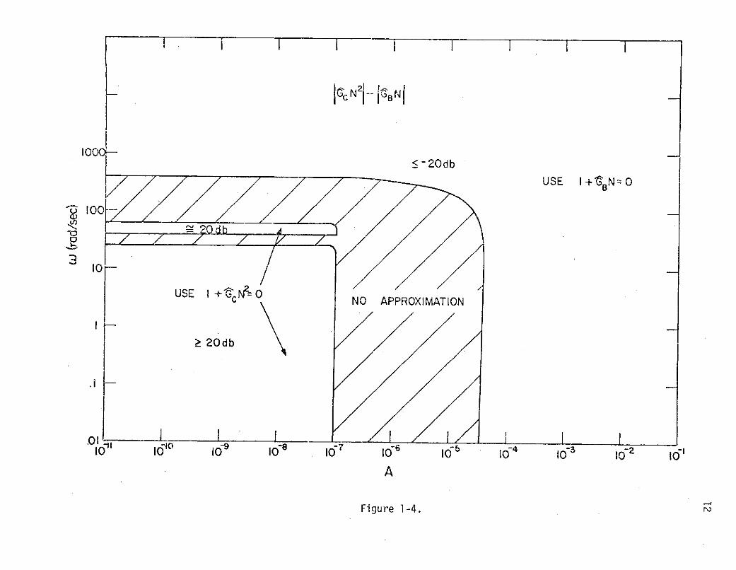
Figure 1-4 illustrates the regions in the w versus A plane in which the

two approximations are valid. The cross-hatched area represents the

region in which no approximation can be made, and the graphical method

cannot be used. The criterion of >20 db and <-20 db is used for

magnitude comparison for significance.

The results of Fig. 1-4 show that the graphical approximation

method is valid for the following ranges of w and A:

1. Use 1 + G = 0 :

A < 10-7 w < 40 rad/sec

and 60 < w < 80 rad/sec

2. Use 1 + GBN = 0

A > 6 x 10-5 m > 600 rad/sec.

For the region of validity of case 1 above, Fig. 1-5 shows the

2plots of GC and -1/N . The heavy portions of the curves indicate the

parts which are valid for stability analysis. Similarly, Fig. 1-6

shows the case when the equation 1 + GBN = 0 may be used for approxi-

mation. Again, the intersection between the heavy portions of the GB

and the -1/N curves would indicate the possibility of self-sustained

oscillation in the two-axis LST system. Since there are no intersections

L Ic IN 2 N

1000-S -20db

USE I+ISN=O

,o -

USE I +cN2= 0 NO APPROXIMATION

20db

IO 110- 1 s I- o o- 1-5 o-4 o-3 I- 1A

Figure 1-4.

13

between the valid curves in Figs. 1-5 and 1-6, the system under study

is stable for the parameter values used. This result will be sub-

stantiated by the two other methods which are discussed in the following

sections.

1-4. A Direct Method of Predicting Self-Sustained Oscillations in

The Two-Axis LST System

A direct but time-consuming method of predicting self-sustained

oscillations in the two-axis continuous-data LST system is to calculate

all the terms in the following stability equation for a wide range of

values of w and A:

1 + GB(jw)N(A) + Gc(jw)N (A) = 0 (1-26)

Although the direct method would be quite tedious, and it is

possible that with a given selected increment of variation for the

values of w and A, the solution runs may still miss the exact solutions,

the results in general will give insight to the appropriate guess on

the initial values for the numerical-iteration method. Therefore, it

is enlightening to investigate this direct approach at this point.

'. 2Figures 1-7 through 1-9 show the plots of GB(jm)N(A) + GC(jw)N (A)

for y = 1.38 x 107, and all the system parameters as given previously,

and for three different sets of values for the coupling coefficients

K2 and K3 . Note that for the three cases illustrated, all the trajectories

for various combinations of A and w do not intersect the critical point

which is at 0 db and -180 degrees. Thus the system is stable. However,

the results show that as the value of K2 is decreased, the trajectories

S= 1.38X 107

-150 -50 36

-160 - 60 20 10 6

70 25 A= IO -.0.01 35

8 eG 34

-170- 28 33

-180 30

I10

-210 o I I I I I I-360 -320 -280 -240 -200 -160 -120 -80 -40 0 40

DEGREES

Figure 1-5.

O = i.38 X 0 7

-60 1- A 6A= 0-

-_0 -4020 1 6 w 0

S-80 5 2

(5x6-90 X200 G

400/N -7-100- X IO57

I 0'7

A=O 600

-110HO

-120 I I I-360 -320 -280 -240 -200 -160 -120 -80 -40 0 40

DEGREES

Figure 1-6.

5j 16

= 1.38x10 7

4 K2= 1000

32 - A= I070

24 - A=10 0 1

CiO

A=5xI 0.120

90

0 - A= 0 0

30

CRITICAL CRITICAL

-24 I I I I

9

-16 A=-

Figure 1-7.

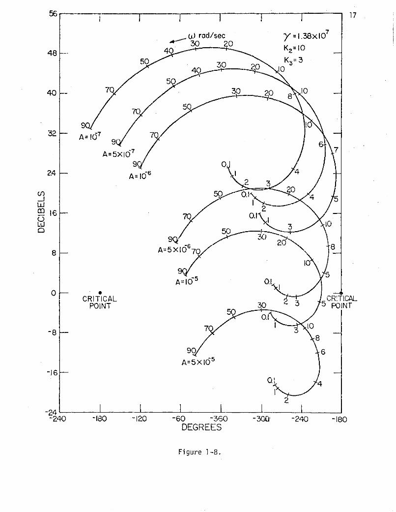
56 ___ I_ _ 17

U0 rad/sec 7= .38x1o30 0

48 4 K50 30 K3 = 3

40- 7 30 8. 10

S5/

32 A= 1 507 7

24 - A= 1 6 , 47

_J

165 0.1LU 30

8 - A= 5 x15'708

A=165 01

CRITICAL CRTICALPOINT 30 3 5 POINT

O.1

8

90

A=5xds-16

2

-24 I I I I -240 -180 -120 -60 -360 -3C -240 -180

DEGREES

Figure 1-8.

565 61 1 I 1 --1 8

'V 1.38X 10--- rod/se

30 O sec K= 0.1

48 4 10 K= 3-

30

'7

40- 620 0

32 A- .5 70-05

A=5xiO 44

3024- A= 16

:50 3 204LW 2- 16-

0100 30 2 3

24 I I I I

- - - -3 5 3 -X4 - -

Figure 1-9.1500.7CRITICAL a CRITICALPOINT .03 POINT

-8 03

01

0.1

-ISO -120 -60 -360 -300 -240 -180 -120DEGREES

Figure 1-9.

19

get closer to the critical point. Figure 1-10 shows the trajectories

when K2 = 0.1 and K3 = 0.1. It is noticed that several trajectories

are very close to the critical point. Figure 1-11 shows a magnified

version of Fig. 1-10 around the critical point. The figure shows that

the trajectories for A = 5 x 10-6, 10-6, 5 x. 10-6, are all very close to

the critical point. This gives indications that there may be more than

one solution. It will be shown in the next section by the numerical-

iterative method that there are indeed two solutions for the stability

equation. One is at A = 5.9867 x 10-7 and w = 1.88 rad/sec, and the

other is at A = 5.07397 x 10-6 and w = 4.1086 rad/sec. These solutions

must still be checked for stable or unstable equilibrium solutions.

1-5. Exact Solution of the Stability Equation by Numerical-Iterative

Techniques

In this section the stability equation developed in Sec. 1-2 is

solved numerically for its exact solutions. The numerical method

utilized has been described in [2] and is found to be quite effective

for the two-axis LST system.

The stability equation, Eq. (1-19), can be written as

1 + GB(jw)N(A) + GC(jw)N 2 (A) = 0 (1-27)

Define

GB(jw) = GR1 + jGI 1 (1-28)

GC(jw) = GR2 + jGI2 (1-29)

N(A) = NR1 + jNl1 (1-30)

30 20 A= ! - 7 y = 1.38x107

48 - 250 20

A=5XI0

A= 1( 640- 2+--0 7

107O 8\ 632 -5 5

/ 0 4

30

L- 10 3o 16 -

8 - 70o8 6

90/ 2

O- CRITICALPOINT /

-8- 10.7

-16- .7

. / 0.8-24 10 / l __

-120 -60 -360 -300 -240 -s180 -120 -EoDEGREES

Figure 1-10.

1\

6-

7 A= AIO A05x1 A= IOy = 1.38x10

4 K2 = 0.1

K3 = 0.1

2

1.6

LW 4

-4

14

-8 0.8-A= 5 xId

-240 -220 -200 -180 -160 140 -120DEGREES

Figure 1-11.

22

N2 (A) = NR2 + jNI2 (1-31)

where GR1, GII, GR2' GI2, NR1I NI1, NR2, and NI2 are all real

quantities.

If Eqs. (1-28) through (1-31) are substituted into Eq. (1-27),

it becomes

1 + (GR1 + jGII)(NR1 +jN I) + (GR2 + jGI 2)(NR 2 + jNI2 ) = 0 (1-32)

When the real and imaginary parts are separated, Eq. (1-32) yields

A = AR + jA I = 0 (1-33)

with

AR = 1 + GRINR1 - GI1NI 1 + GR2 NR2 - GI2 NI2 = 0 (1-34)

and

AI = GI1NRI + GR1NIl + GI2NR2 + GR2 NI2 = 0 (1-35)

Further simplification is possible in Eqs. (1-34) and (1-35)

if we recognize that NR2 + jN12 = (NRl + jNI )2 but is not necessary

since the solution of Eqs. (1-34) and (1-35) will be performed on a

digital computer.

Equations (1-33) and (1-34) represent two equations in the two

variables w and A. As before [2], let us define

x= [3 (1-36)

23

RF = (1-37)

AI

Then, Eqs. (1-34) and (1-35) can be written as

F(x) = 0 (1-38)

The Newton-type quadratically convergent numerical method

described in [2] can now be directly applied to this two-variable

system.

To initiate the iterations, an initial solution is needed. The

results of the direct calculation method, presented in the previous

section provide an adequate initial solution. As in that section, the

parameters which need to be varied are K2 and K3. Once a solution for

a given value of K2 and K3 is known, K2 and/or K3 could be changed

slightly and the new solution is obtained by using the old solution

as the initial guess for the new system.

With K2 and K3 set to very small values, the system is decoupled,

and the solution of the single-axis LST system could be used as an

initial guess for that of the two-axis LST system.

If K2 = 0.1 and K3 = 0.1, the results from the direct calculation

method shown in Figs. 1-10 and 1-11 indicate that two possible solutions

exist. The approximate amplitudes and frequencies of the solutions are

Solution No. 1 w = 5 rad/sec

A = 5 x 10-6 rad

Solution No. 2 m = 2 rad/sec

A = 1 x 10-6 rad

24

With these approximate solutions as initial conditions, the results

of the numerical iteration procedure are obtained and tabulated in the

first set of iterations in Fig. 1-12 and Fig. 1-13. These iterations

indicate that the actual solutions are

Solution No. 1 w = 4.1086 rad/sec

A = 5.0739 x 10-6 rad

Solution No. 2 w = 1.88 rad/sec

A = 5.99 x 10-7 rad

Figures 1-12 and 1-13 also show the change in the solutions when

K2 and K3 are reduced to K2 = K3 = 0.01 and K2 = K3 = 0.001, respectively.

As mentioned previously, the initial guess for a new set of values of

K2 and K3 is the solution with the previous values of K2 and K3.

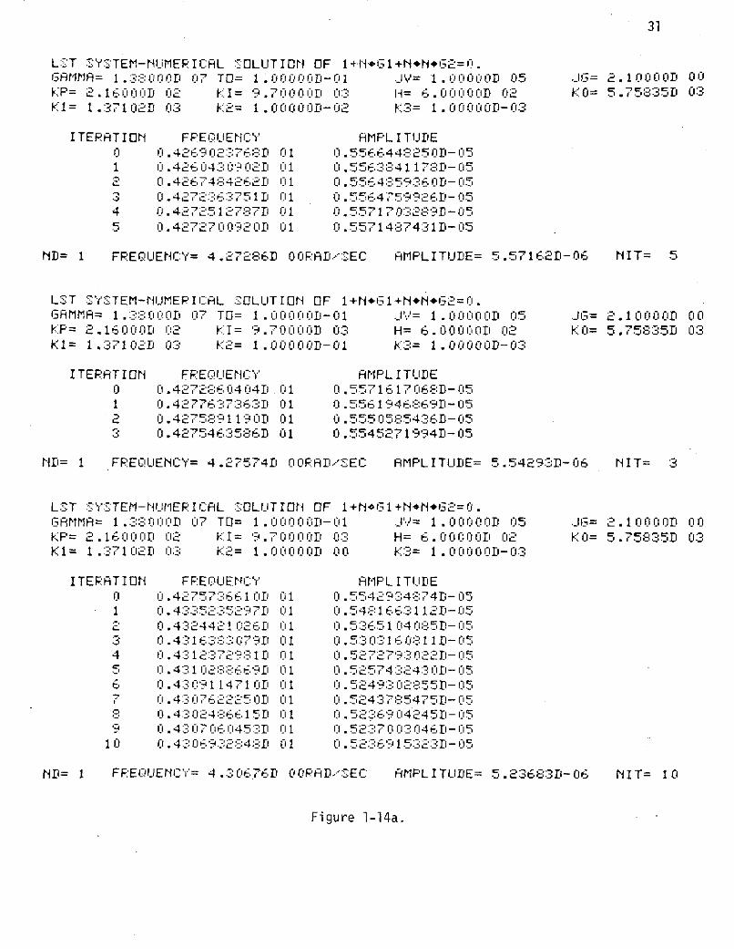
With K3 fixed at 0.001, if K2 is increased (Figs. 1-14 and 1-15),

the solutions will change, until K2 = 8 for solution no. 1 and K2 = 7

for solution no. 2, beyond which no solution is obtained. It is

interesting to note that the two solutions move closer together with

increasing K2 and almost merge into each other before disappearing

altogether. The result is analogous to lowering the G(jw) curve or

raising the -1/N curve in the single-axis case.

It can be concluded that for K3 = 0.001, K2 should be less than

8 for a sustained oscillation to occur. In fact, with K2 = 8 (solution

1) and K2 = 7 (solution 2) the roots of the stability equations do not

appear to have converged adequately, and well defined roots occur only

for lower values of K2. A maximum of 20 iterations are attempted before

the numerical process is terminated.

If K3 is kept fixed at 0.2 and K2 is varied, the iterations in

25

Figs. 1-16 and 1-17 show that K2 can be increased only up to K2 = 3

for solutions to be obtained.

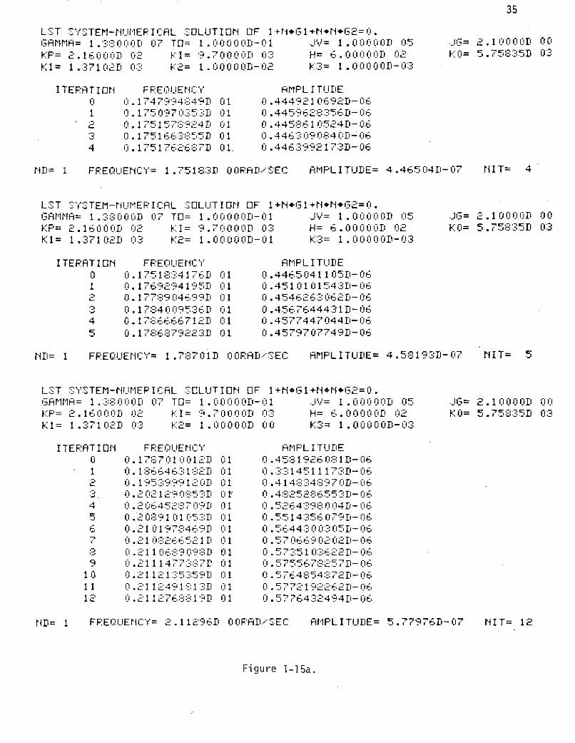
On the other hand, K2 can be kept fixed and K3 varied; these results

are shown in Figs. 1-18 through 1-25. In Figs. 1-18 and 1-19 K2 is

fixed at 0.001, and the maximum value of K3 for a solution to the stability

equation is approximately K3 = 0.4 for solution no. 1 and K2 = 0.3 for

solution no. 2. With K2 = 0.1, 1.0 and 5.0, the maximum values of K3 are

0.4 (solution 1 and 2), 0.3 (solution 1 and 2) and <0.1 (solution 1 and 2),

respectively. These results are shown in Figs. 1-20 through 1-25.

Table 1-1 summarizes all the results. In the table, the solutions

for K2 = K3 = 0 are the solutions with the single-axis LST system. It is

seen that when K2 and K3 are very small, the solutions of the two-axis

system approach those of the single-axis system.

The data in Table 1-1 can be used to plot the region in the K2 - K3plane in which sustained oscillation can exist. Figure 1-26 shows this

region. For values of K2 and K3 outside the crosshatched area, no

sustained oscillations should exist.

The motion of the roots with variable K2 and K3 are plotted in

Fig. 1-27, using the data in Table 1-1. The points marked K2 = 0,

K3 = 0, represent the single-axis LST system solutions. The solid closed

regions represent the regions of root movements where reliable convergence

was obtained. The dotted lines include the regions where reliable

convergence of the iterative scheme was not obtained with 20 iterations,

and, which can be considered as a boundary area between existence and non-

existence of solutions. Note that in Fig. 1-27 the two solutions are

farthest apart when K2 = K3 = 0. Figure 1-27 also shows how the two

26

solutions tend to merge just before the solutions disappear.

27

Table 1-1

ROOT #1 ROOT #2

K2 K3 FREQUENCY AMPLITUDE FREQUENCY AMPLITUDE

0.1 0.1 4.1 5.07 x 10- 6 18 5.99 x 10- 7

0.01 0.01 4.26 5.52 x 10- 6 1.76 4.58 x 10- 7

0.001 0.001 4.27 5.56 x 10-6 1.75 4.45 x 10

0.0 0.0 4.27 5.57 x 10- 6 1.75 4.45 x 10- 7

0.01 0.001 4.27 5.57 x 10-6 1.75 4.46 x 10- 7

0.1 0.001 4.28 5.55 x 10- 6 1.79 4.59 x 10-7

1.0 0.001 4.31 5.24 x 10-6 2.11 5.79 x 10- 7

-6 -72.0 0.001 4.34 4.91 x 10 6 2.43 7.17 x 103.0 0.001 4.36 4.56 x 106 2.73 8.69 x 10-

4.0 0.001 4.38 4.20 x 10- 6 3.01 1.04 x 10- 6

5.0 0.001 4.37 3.81 x 10- 6 3.29 1.25 x 10- 6

6.0 0.001 4.34 3.35 x 10-6 3.58 1.53 x 10-6

7.0 0.001 4.19 2.6 x 10-6 3.97** 2.06 x 10- 6**

8.0 0.001 3.95** 1.50 x 10- 6** -

1.0 0.001 4.31 5.24 x 10- 6 2.11 5.79 x 10-7

1.0 0.01 4.29 5.19 x 10- 6 2.23 5.93 x 10- 7

1.0 0.1 4.13 4.74 x 10- 6 2.12 7.71 x 10- 7

-6 -

1.0 0.2 3.91 4.18 x 10- 6 2.39 1.03 x 10- 6

1.0 0.3 3.62 3.47 x 10- 6 2.62 1.43 x 10- 6

1.0 0.4 - - 3.2** 2.57 x 10- 6**

5.0 0.001 4.37 3.81 x 10-6 3.29 1.25 x 106

5.0 0.01 4.34 3.72 x 10-6 3.31 1.30 x 106

5.0 0.1 5.46** 7.13 x 10- 6** 3.75** 2.25 x 106**

1.0 0.2 3.91 4.17 x 10-6 2.39 1.04 x 10- 6

2.0 0.2 3.85 3.85 3.64 x 10- 6 2.79 1.37 x 10- 6

3.0 0.2 3.69 2.86 x 10- 6 3.28 1.95 10-6

0.001 0.001 4.27 5.57 x 10-6 1.75 4.45 x 10- 7

0.001 0.01 4.26 5.54 x 10- 6 1.76 4.56 x 10- 7

28

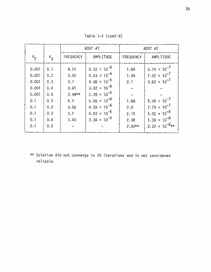
Table 1-1 (cont'd)

ROOT #1 ROOT #2

K2 K3 FREQUENCY AMPLITUDE FREQUENCY AMPLITUDE

0.001 0.1 4.11 5.12 x 10-6 1.84 5.79 x 10- 7

0.001 0.2 3.92 4.63 x 10-6 1.95 7.52 x 10- 7

0.001 0.3 3.7 4.08 x 10-6 2.1 9.82 x 10- 7

0.001 0.4 3.41 3.42 x 10-6

0.001 0.5 2.94** 2.39 x 10-6 -

0.1 0.1 4.1 5.08 x 10-6 1.88 5.98 x 10- 7

0.1 0.2 3.92 4.59 x 10-6 2.0 7.79 x 10- 7

0.1 0.3 3.7 4.03 x 10- 6 2.15 1.02 x 10- 6

0.1 0.4 3.40 3.34 x 10- 6 2.38 1.39 x 10- 6

0.1 0.5 - 2.82** 2.22 x 10- 6 **

** Solution did not converge in 20 iterations and is not considered

reliable.

29LST SYSTEM-NUMEPICAL SOLUTION OF 1+N*GI+NI*N*G2=0.GAMMA= 1.38000D 07 TO= 1.0000oD-01 JV= 1.00000D 05 JG= 2.10000D 00KP= 2.160001 02 KI= 9.70000D 03 H= 6.00000D 02 KO= 5.75835D 03Kl= 1.37102D 03 K2= 1.00000D-01 K3= 1.00000D-01

ITERATION FREOLUENCY AMPL ITUDE0 0.5000000000D 01 0.5000000000D-051 0.47:33762972D 01 0.5433071349D-052 0.4 5 26 5 62584D 01 0.5454333473D-053 0.4375323004D 01 0.5360015536D-054 0.4270975962D 01 0.5259907533D-055 0.4203232573D 01 0.518:3187.32D- 056 0.4161323855D 01 0 .5132000356D-057 0.41:-:6226451f 01 0.5100190831D-058 0.4121313005D 01 0.5080665473D-059 0.4111573450D 01 0.5066187720D-05

10 0.4125227288D 01 0.5118030600D-0511 0.4115488437D 01 0.5099437398D-0512 0.4104483976' 01 0.5075156770D-0513 0.41089510551' 01 0 .5075090383D- 0514 0.4108776583D 01 0.5074449931D-05

ND= 1 FREQUENCY= 4.10860D OORAD/SEC AMPLITUDE= 5.07397D-06 NIT= 14

LST SYSTEM-NUMERICAL SOLUTION OF 1+N*GI+N*N*G2=0.GAMMA= 1.38000D 07 TO= 1.00000D-01 JV= 1.00000D 05 .JG= 2.10000D 00KP= 2.16000D 02 KI= 9.70000D 03 H= 6.00000D 02 KO= 5.75835D 03K1= 1.37102D 03 K2= 1.000001-02 K3= 1.O0000D-02

ITERATION FREQUENCY AMPLITUDE0 0.4108597203D 01 0.5073966584D-051 0.4168820145D 01 0.5248288860D-052 0.4205531785D 01 0.5364353532D-053 0.4226335066D 01 0.5432259787D-054 0.42379364721D 01 0.547066:3581D-055 0.4244508200 01 0.5492764659D- 056 0.4246721288D 01 0.5477545295D- 057 0.4253298522D 01 0.5511028750D-058 0.4253818862D 01 0.5517540846D-059 0.4253573182D 01 0 .552260793 O D-05

10 0.4262696521 01 0 .5520588880D-0511 0.4255 858006' 01 0.5512477452D-0512 0.4255246471D 01 0.5516839666D-05

ND= 1 FREQUENCY= 4.25522D OORAD/SEC AMPLITUDE= 5.52114D-06 NIT= 12

LST SYSTEM-rUMEPICAL SOLUTION OF 1+N*G1+N*N*G2=0.GAMMA= 1.38000D 07 TO= 1.00000D-01 JV= 1.000001 05 JG= 2.10000D 00KP= 2.16000D 02 KI= 9.70000D 0:3 H= 6.00000D 02 KO= 5.75835D 03K1= 1.37102D 03 K2= 1.00000D-03 K3= 1.00000D-03

ITERATION FREQUENCY AMPL I TUDE0 0.4255217:24D 01 0.5521142485D-051 0.42606764241' 01 0 .554279581 8-052 0.425653481 6D 01 0.5327:396968-- 053 0.4252613070D 01 0.5420675622B-054 0.4261846964r 01 0.54965176:30D-055 0.4266693459D 01 0.5536135509D-056 0.4269530544 01 0. 5557835647D-057 0.4269042818D 01 0.5561545739D-05

ND= I FREQUENCY= 4.26902D OORAD'SEC AMPLITUDE= 5.56645D-06 NIT= 7

Figure 1-12.

30LST :SYSTEM-NUMER I CAL :S OLUTION OF 1 +N*G 1 +NoN*G2= 0.GATMMA= 1.:38000D 07 TO= 1.0000D-01 JV= 1.000l1D) 05 JG= 2.1I000D 00KP= 2.16000D 02 KI= 9.70000ID 03 H= 6.00000D 02 KO= 5.75835D 03Kl= 1.37102D 03 K2= 1.0000D-01 K3= 1 . 0 O- 01

ITERATION FREQIUENCY AMPL I TUDE0 0.200000000 01 0 .100l000000D-051 0.184923024D 01 0.6242848602D- 062 0.1852950575D 01 0.5882981170 D- 063 0.1:867139 237I 01 0.593 :0626214D-064 0.1874829545D 01 0.59622728061-06

.5 0.1878890231D 01 0.59791 38586D- 066 0.1 8800101 1D 01 0. 5979328: 084i- 067 0.1880201 346 01 0 . 5986 1 59:' 1 D -8 0.18803343:50 01 0.5986705996D-06

ND= 1 FFREQUENCY= 1.88 :304D 00RAD/SEC AMPLITUDE= 5.98:812D-07 NIT= 8

LST :SYSTEM-NUMERICAIL SOLUTION OF 1+NGI+N1*N*.G2=0.GAMMA= 1.38000D 07 TO= 1 .00000D-01 .JV= 1.00000D 05 G= 2.10000D 00KP= 2.16000D 02 KI= 9.700001 03 H= 6.000001D 02 KO= 5.75835D 03K 1 = 1.371 02 03 K2= 1.0000D-02 K:3= 1 . 00000 D-02

I TERATION FREQUENCY AMFMPLITUDES 0.1880421807D 01 0.59881184 4D- 061 0. : 186575499D 0'1 0.52147436 :08D'- 062 0.1787791 1116 01 0.4874 09032D- 06I3 0. 1i774 0714:80D 0 1 0.472' :0024797D- 064 0.17673 10255 01 0. 4645:333492D-065 0.1763726929D 0 1 0 .46 0587842:3D-066 0.1758874217D 01 0.4525793409D- 067 0 . 175:88:12030: ' 01 '0.4613:8:77E 605D- 68 0. 1 758882166D 0 1 0 .458:30 95382D- 6O9 0.1759606827D 01 0.4577612065D-06

10 0.175961728371 01 0.45:31187707D-06

ND= 1 FREQ!UENCY= 1.75963D OORAD/SEC AMPLITUDE= 4.58:129D-07 NIT= 10

LST SYSTEM-NLIUMER I CAL SOLUTION OF 1 +*G 1 +N*N*G2=0.GAMMA= 1.38000D:' 07 TO= 1.O00-01 JVI= 1.00000 05 .JG= 2.10000D i00KP= 2.16000D 02 KI= 9.70000' 03 H= 6.0L'000D 02 KO= 5.75835D 03K 1= 1.:37102D 03 K2= 1.00 D-03 K3= 1.00000 - 0:3

ITERATION FREQUENCY AMIPLITIUDE0 0.17596:34012 D 0'11 .458 1 286762D- 061 0. 1754793059 01 0.4515838346D - 062 0.17520968-24D 01 0.44 1194314D-063 0 . 1743:716 093D 0 1 0.4323366512D-- i4 0.17447852 1 0' 1 0.44 3176104 D- i65 0.1746624895D 01 0.44232708861-066 . 17471 72576D 01 0.44366758:32D-067 0.1747595835D 01 0.444257:8928D-068 0.1747828656D 01 0.44467658:61D-06

IND= 1 FREIUE'NCY= 1.74799D OORAD/SEC AMPLITUIE= 4.44921D-07 NIT= 8

Figure 1-13.

31

LST SYSTEM-NUMERICAL SOLUTION OF 1+NHGI+N*N*G2=0.G'AMMA= .138:000D 07 TD= 1.0000OD-01 JV= 1.000(0D 05 JG= 2.10000D 00KP= 2.16000D 02 KI= 9.70000D 0:3 H= 6.0OOD 02 KO= 5.75835D 0:3Kl= 1.37102D 03 K2= 1.O00030-02 K3= 1.0000oD-0:3

ITERATION FREQUENCY AMPL ITUDE0 0.4269023768 01 0. 5566448250D-051 0.42604:30902 01 0.556384117D- 052 0.4267484262D 01 0.556485936D-053 0.4272363751 01 0.5564759926D-054 0.4272512787D 01 0.5571703289D-055 0.4272700920 01 0.5571487431D-05

ND= 1 FREQUENCY= 4.27286D OORAD:SEC AMPLITUDE= 5.57162D-06 NIT= 5

LST SYSTEM-NUMERICAL SOLUTION OF 1+N*G1+NN'2=0.GAFMMA= 1.38000DOf 07 TO= 1.0000O-0I1 J.V= 1.00000 05 JG= 2.1000D 00KP= 2.16000r 02 KI= 9.70000 03 H= 6.0000:oI 02 KO= 5.75835D 03Kl= 1.37102D 03 K2= 1.0000OD-01 K3= 1.00000D-03

I TERAT ION FREQUENCY AMPL I TUDE0 0.4272860404D 01 0.55716170618D:- 051 0.4277637363D 01 0.5561946869- 052 0.4275891190D 01 0.5550585436D-053 0.4275463586.D 01 0.5545271994D- 05

ND= 1 FREQUENCY= 4.27574D OORAD/SEC AMPLITUDE= 5.54293D-06 NIT= 3

LST S'YSTEM-NUMERICAL :SOLUTION OF 1+N*GI+NN*6G2=0.GAMMA= 1.3800:0 07 T0= 1.0000D-01 JV'= 1.00000D 05 JG= 2.10000D 00KP= 2.16000 02 KI= 9.70000D 0:3 H= 6. 00000 02 K 0= 5.75835D 03K1= 1.37102D 0: K2= 1.00000D 00 K3= 1.0000O'-0:3

ITERATION FREOUENCY AMPLITUDE0 0.4275736610D 01 0. 554293474D-051 0.4352-:5297D 01 0.54:166 3112D-052 0.4324421 026D 01 0.5 I3651 04085D- 053 0.43163810791 01 0.5303160811D-054 0.4312372981D 01 0.5272793022D-055 0.431 02886::69D 01 0.5257432430D-056 0.4309114710i 01 0.52493028:: :55D- 057 0.430 622250 01 0.524:3785475D-058 0.4302486615D 01 0.52:36904245D-059 0.4 I 307060453D 0 1 0.5237003046D-05

10 0.4069-32848D 01 0.52:369153:3D-05

ND= 1 FREQUENCY= 4.30676D OORAD-'SEC AMPLITUDE= 5.23683D-06 NIT= 10

Figure 1-14a.

32

LET SYSTEM-NUMERICAL :CLUTION OF 1+H*G1+N*N*62=0.GAMMA= 1.38000D 07 TO= 1.0000aD-01 JVV= 1.000I:00 05 ._JG= 2.1000 D 00KP= 2.16'00D 02 KI= 9.70000D 03 H= 6.00000D 02 KO= 5.758:35D 03.Kl= 1.37102D 03 K= 1.00000D 00 K3= 1.00000D-0:3

I TERAT ION FREOUENC,' AMPLITUDE0 0.4300000000r 01 0.5200000IOOD-05

1 0.4 :3052 81886D 01 0.52283 01D- 052 0.4305283850D P 01 0 .522245349D- 053 0.4308744-870D 01 0 .524574872D-054 0 .4308:6.34.35:3: 01 0.54:3241 015D-05

ND= 1 FREQUENCY= 4.30865 O00RFIADSEC AMPLITUDE= 5.24185D-06 NIT= 4

LST S"YSTEM-NUMERICAL SOLUTION OF 1+N*I1+N*NG2=0.GAMMA I.:_000D 07 TO= 1 .0000D-01 JV= 1.O0000oD 05 .JG= 2.1000D 00KP= 2.16000D 02 KI= 9.70000 D 03 H= 6 .o0o000 02 KO= 5.758:335D 0:3Kl= 1.37102D 0:3 K2= 2.0001) 00 K3= 1.000000-03

ITERATION FIREQUENCY AMPLITUDE0 0.43 08645 1 93D 01 0 5241 850229D-051 0.4375960005D 01 0.5185863190D-052 0.4360035 00D- i 0.5047331412D-D05:3 0.4349924772 01 0.4976486582 D - 054 0.4344905380D 01 0.4941913249D-055 0.4342313852D 01 0.4924475958D-05

.6 0.4340863107D 01 0.4915247605D-057 0.439884:306D 01 0.49 0994755OD-058 0.43:39062983D 01 0 .4906586223D-05

ND= 1 FREQUENCY= 4.3:3810D ORAD/.SEC AMPLITUDE= 4.90415D-06 NIT = 8

L:T ':STEM-NUMERICAL SOLUTION OF I+N*G1+N*N*62=0.GAMMA= 1.3800D 07 TO= 1.00000D- 01 JV= 1. 000010 05 JG= 2 . 1 0000D 00KPF= 2.16000 02 KI= 9.70000D 03 H= 6.00000D 02 KO= 5.75835D 0:3K1= 1.37102D 03 2'= 3.0000O 00 K:3= 1.0 O0000D-03

ITERATIO rN FREQU IE NCY AMPL ITUDE0 0.4338100273D 01 4 0.490415210%D-051 0.440 i7947:3:30 01 0.48610091 D- 052 0.43873::3490 01 0.4711098352D-053 0.4375506949D 01 0.46:3630 1815D-i054 0.436 9644072 01 0.459994927D-055 0-.4366618831 01 0.4581578394D-056 0.4364918225D 01 0.4571778521D-057 0.4363815507D 01 0.4566133105 - 058 0.462939491D 01 0 .4562548417D-05

ND= 1 FREQUENCY= 4.36199D OORAD/SEC AMPLITUDE= 4.55997D-06 NIT= 8

Figure 1-14b.

t' L eain6yj

6 =±IH 90-M1.t99C E: zGrIldwH 03S.-GM400 11IS~t' t =.XCk3riO3I T =04l.

TO IC'Q:ET'O9?WO E.l

90-11 C'T990SW' ToR M862VTISM I

goWMP aW TO GevWWWW4t-t-- IGOU IM W C 0 TI:vt9G:?:~ 5' I

gC'-G5196E:9 8LI TO U69CM)Z9' 1' I

00 GO M =9F go aoIooC Or 11t'2CI'O-.l =0i Zo GIISW 6

_oa~~wT~~ IC woui' IWOMAWW3SA -t'

60'l!ET =1- IIano nanmm 03W196?9 =3%0 I' Cl C

gL-I1T1689OP ITO GFE0I 1,99C'-4't' E.

&O-MOFETEWW To t9*9E611 0Cl~LO tg0-1E.:2:6C 6C01 TO UMLI 10 11'1t4,

&0 -G8162WA0?t'6 1Et l I0 G0t698929VVYl T'';0 -'191 '6'E;E,,". TO 1 0 19.0 T'EVt 0

0I A -11t':04bA Li I jQI I::S I't'I C

:E:0-110001:10 =C:A 00 110:111:1 's =jA Co0 11?O IPT. = I ACo QQ68SY9 =ON 2 O ' I0 G OO t9 =H C60 UCICt l 0 6 M I0 GOMM'C'0 l4 =d''q0o uol o =or0 0 EF 0 OOO'sCIT =A 1t;-QOOCI 0 ' i =0± ZCI U1:06t: s IC i btwwu

I)='E*~4H+El so+ wouno IOWlOC ~CIMAWfl-W31S.,J 121

34

L:T S'3Y:TEM-NUMER I.CL SOLUTION OF 1 I+'*1 +l.l+.3G2=0.GAMMA= 1 .3:8000D '07 TO= 1 .0000Of-01 JV= 1.00000 05 JG= 2.10000 00KP= 2.16000D 02 KI= 9.70000D 03 H= 6.00000D 02 KO= 5.75835D 0:3Kl= 1.:37102D 0:3 K= 7.00000 00 K:3= 1.0000OD-03

ITERATION FREQUENCY AMPLITUDE0 0.434012381D 01 0.:3:346473:3'73DT- 051 0.44086;45049' 01 0 .332578975 8D- 052 0.4325 039146D 01 0.301597257D-05:3 0.42.62701797D 01 0 .2828294047D-054 0.4 233- 1 82205D 01 0.2738989086:':: :3D-055 0. 42165 061D 01 0.2688925065 -056 0.4204935:306D 01 0.2655545194D1- 057 0.41'7896293 01 0 .6:34 100150-058 0.4188751327D 01 0.2612619774D-059 0.4189724044D 01 0.2606441657D-05

10 0.4191211536D 01 0.2604446450D-05

ND= 1 FREQUENCY= 4.19137D OOPADLSEC AMPLITUDE= 2.60430D-06 NIT= 10

LST SYSTEM- LNUMER ICAFL SOLUT IN OF 1 +N*G 1 +N*N*G2= 0.GAMMA= 1.8:000D 07 TO= 1.0000r0D-01 J'V'= 1.000001 05 JG= 2.10000D 00KP= 2.16000D 02 KI= 9.70000D 0:3 H= 6.00000D 02 KO= 5.758351) 0:3Kl= 1.37102D 0:3 K2= S.00000rD o0 K:3= 1.000 oD-03

ITERATION FREQUENCY AMPLITUDEo 0.4191 366586D 01 0.2604300965D-051 0.4320830567D 01 0.2755449920D-052 0.3885654674D 01 0.1537227546D-053 0.3992688964F 01 0.1777098203D-054 0.410 1211 254 D 01 0.20 '18197669D- 055 0.4049068 :157D 01 0.2133752715- 056 0.4218650868D 01 0.244280 ,8016D - 057 0.5:328:541 :0:39 01 0.5121 54:2808 :D-058 0.49323 :74097D 01 0.4 09 0391- 1D-059 0.458072990D 01 0.2898763-479D-05

1 0 0.4272683 11 7 01 0.2338930959D-0511 0.4726012700D 01 0.3527236013D-0512 0.46424620:32 01 0.2206214287D-0513 0.41 02385161D 01 0.1712607528D- 0514 0.4511000940D 01 0.2807657101D-0515 0.4185049'431 01 0.2143 -99524 0oD- 0516 0.4337921541r 01 0.25663--.,85 797PD-0517 0.4584719 '291 01 0.17296064D- 0518:: 0.441:031316D 01 0.25 9 417e 16-0519 0. : 390153 7201D 01 0.1457090202D- 0520 0 .395155389 01 0.1500036479D-05

ND= 1 FREQUENCY= 3.95136D OORAD/SEC AMPLITUDE= 1.50004D-06 NIT= 20

Figure 1-14d.

35

LST SYSTEM-NUMERICAL SOLUTION OF 1+H G1+N*N*G2=0.GAMMA= 1 .:3:00 10 07 TO= 1.000 -01 JV= 1.000 00 05 J._G= 2. 100 00 00

KP= 2.16000D 02 KI= 9.70000D 03 H= 6.00'OOD 02 KO= 5.7535D 03

K1= 1.37102D 03 K2= 1. 0000 OF- 02 K3= 1. 0000 - 03

ITERAT I ON FREUENCY AMPL ITUDE0 0.1747994849D 01 0.4449210692D-061 0.175097 035:-D 01 0.445962356D- 062 0.1751578924D 01 0.4458610524D-063 0.1751 .:663855fD 01 0.446:3090 84 -6I 64 0.1751762667 01. 0.4463992173D-06

ND= 1 FREQUENCY= 1.75183D 00RAD/SEC AMPLITUDE= 4.46504D-07 NIT= 4

L:ST SYSTEM-INUMERICAL S:OLUTION OF I+N*GI+N*-N-2=0.GAMMA= 1.38000D 07 TO= l.00'iOiF-''-01 JY= 1.00 IOOO 05 JG= 2.1000O'D 00KP= 2.160001 02 KI= 9.70000D 03 H= 6.000001' 02 KO= 5.75835D 03

K1= 1.371021D 0:3 K2= 1 .00 OOD-01 K3= 1 .00000-03

ITERATION FREOUEHNCY AMPLITUDE0 0.1751834176D 01 0.4465041105D-061 0.1769294195D 01 0.4510101543Di-062 0.1778904699D 01 0.4546263062D-063 0.1784009536D 01 0.45676444431D-064 0. 1786666712D 01 0 .4577447044D-065 0.1786879223D 01 0.4579707749D-06

ND= 1 .FREQUENCY= 1.78701fl OORA./SEC AMPLITUDE= 4.58193D- 07 NIT= 5

L:T SYSTEM-NUMERICAL SOLUTION OF 1+NGI+Nr*+N62=0.GAMMA= 1. :l38000D 07 TO= 1. 0 00D-01 .JY= 1.0000 0 05 JG = 2 .10000D 00KP= 2.1600D 02 KI= 9.70000D 0:3 H= 6.00000Do 02 KO= 5.75835B 03K1= 1.371021D 0:3 K2= 1.000OOD 00 K3= 1.0000OID-03

ITERATION FREQUENCY AMPLITUDE0 0.1787010012D 01 0.45819 26081D-061 0. 1866463182 01 0.3314511173D- 062 0.19539'99120 01 0.414 348970D-063 0.2021290853D O' 0.4 825286553D- 064 0.2064528709D 01 0.564398004D- 065 0.20' 910105:3: 01 0.551435 079D-: '066 0. 21019 78:469D 01 0.5644300 05 D-067 0.2108266521D 01 0.5706690202D-68 0.2110689098D 01 0.57351 0:3622 D- 069 0.21114 77387 01 0.5755678257D-06

10 0.21 12135359 01 0 .5764854872D-011 0.2112491813D 01 0.5772192262D-0612 0.21 12768819D 01 0.5776432494D-OE.

ND= 1 FREQUENCY= 2.11296D 0O0RAOF."SEC AMPLITUDE= 5.779760-07 NIT= 12

Figure 1-15a.

LST SYSTEM-NUMERICAL SOLUTrIN OF L+N1+N*NG2=0. 3bGAMMA= 1.3800C0 C7 T= 1.000000D-O1 JV= L.00000 05 JG= 2.100n00 00KP= 2.160000 C2 KI= 9.70CCOD C3 H= 6.00000D 02 KO= 5.75835D0 03Kl= 1.37102D 03 K2= 1.000000 00 K3= 1.000000-03

ITERATION PREQUENCY AMPLITUDE0 0.21000000000 01 0.58000000000-061 0.21058192380 01 0.57644082180-C062 0.21106834450 01 0.57779394370-063 0.21134006370 01 0.57848853980-064 0.21134585760 01 0.57875519580-06

ND= 1 FREOUENCY= 2.113520 OORAD/SEC AMPLITUDE= 5.788290-07 NIT= 4

LST SYSTEM-NUMERICAL SOLUTION OF 1+N*Gl+N*N*(G2=O.GAMMA= 1.380000 07 TO= 1.000000D-01 JV= 1.000000 05 JG= 2.100000 00KP= 2.160000 C2 KI= 9.7C0000 03 H= 6.000000 02 KO= 5.758350 03Kl= 1.371020 03 K2= 2.000000 CO K3= 1.000000-03

ITERATION FREOUENCY AMPLITUDE0 0.21135223680 01 0.57882942720-06I 0.21987837660 01 0.47457342560-062 0.22862730950 01 0.5541505311D-063 0.23516917170 01 0.62337062680-064 0.2392340682C 01 0.66771529620-065 0.2414543718 01 0.6919494671D-066 0.24255743730 01 0.70374038480-067 0.24303515400 01 0.7C887856150-068 0.24318808540 01 C.71202441000-069 0.24328393040 01 C.71389960070-06

10 0.24334826530 01 C.7151060900-0611 0.24339354860 01 C.71593866780-0612 0.24342705380 01 0.71653880260-06

NO= 1 FREOUENCY= 2.434530 OOAD/SEC AMPLITUDE= 7. 16991D-07 NIT= 12

LST SYSTEM-NUMErICAL SOLUTICN CF I+N*GI+N*N*G2=0.GAMMA= 1.380000 07 TO= 1.00000D-01 JV= 1.00000D 05 JG= 2.100000 00KP= 2.160000 02 KI= 9.700000 03 H= 6.000000 02 KO= 5.758350 03K1= 1.371020 03 K2= 3.00000C 00 K3= 1.00000-03

ITEPATICN FREOUENCY AMPLITUDE0 0.24345273020 01 C.71699083600-061 0.25307037250 01 0.67539179420-062 0.26150496680 01 C.74730169010-063 0.26718189570 01 C.8C575802490-064 0.27038492980 01 0.8395671944D-065 0.27198198200 01 C.8557534471D-066 0.2726656058r0 01 C.8617656 173r)-067 0.27281734610 01 0.8 390060490-068 0.27289191170 01 C.86589763960-069 0.27296032510 01 0.86694999620-06

10 0.27300454510 01 C.8679340734D-0611 0.27304218240 01 C.86858662080-C6

NO= I FPECU'JENCY= 2.730710 OOPArO/SEC AMPLITUDE= 8.691500-07 NIT= 11

Figure 1-15b.

LST SYSTEM-NUMCR ICAL SOLUT!ON OF 1+N*Gl+N',NG2=0.GA4MA= 1.380C00 C7 TO= 1.000000-01 JV= 1.00000D 05 JG= 2.10COOD 00

KP= 2.16000D 02 KI= 9.700000 03 H= 6.000000 02 KO= 5.758350 03

K1= 1.371029 03 K2= 4.00J00 00 K3= 1.000000-03

ITEPATION FREOIUENCY AMPLITUDE0 0.27307112410 01 0.86914988900-06

1 0.28327612720 01 C.8690562992D-062 0.29140723690 01 C.94044174 4 7 0- 0 6

3 0.29652J75090 01 0.95312303330-064 0.2992799595D 01 0.10217814520-055 0.30063065160 01 0.10348693960-05

6 0.30111433820 01 0.10380019380-057 0.30116053060 01 0. 1 C4028 54610-058 0.30122946140 01 0.10409166020-05

9 0.3012666960 01 0.1041986665C-0510 0.30130411490 01 O.1C42589602D-05

ND= 1 FREQUENCY= 3.013330 OORAD/SEC AMPLITUDE= 1.04321D-06 NIT= 10

LST SYSTEM-NUMERICAL SOLUTION OF 1+N*GI+N*N*G2=0.GAMMA= 1.38CCOD C7 TO= 1.003000-01 JV= 1.00000D 05 JG= 2.10000D 00

KP= 2.160000 02 K I= 9.700000 03 H= 6.00000D 02 KO= 5.75835D 03

K1= 1.371020 03 K2= 5.000000 00 K3= 1.000000-03

ITEPATICN FREQOEJNCY AMPLITUDE

0 0.30133297290 01 0.1043207423D-051 0.3115895948D CL 0.1C659922250-052 C.31957166540 01 0.11425688390-05

3 0.3245957530C 01 0.11987198770-054 0.32735744710 01 0.12301918900-055 0.3286982993D 01 0.1244194422D-056 0.32899643840 01 0.12456812450-057 0.32904455500 01 0.12487315320-058 0.32913330090 01 0.12493769450-059 0.32917659820 01 0.1250826172D-05

10 0.32922447670 01 0.1251583502D-05

NO= 1 FREQUENCY= 3.292610 OORAD/SEC AMPLITUDE= 1.252440-06 NIT= 10

Figure 1-15c.

LST SYSTEM-NUERICAL SOLUTION OF 1+N*G+NN*G2a=O.

GAMMA= 1.38Cr00 07 TI= 1.0000OD-01 JV= 1.000000D 05 JG= 2.100000 00

KP= 2.160000 02 KI= G.700000 03 H= 6.000000 02 KO= 5.758350 03

KL= 1.371020 03 K2 = 6.COOCOD 00 K3= 1.000000-03

ITERFAT ION FREOIJENCY AMPLI TUDE0 0.32926089030 01 0.12524417490-05

1 0.33931182040 01 0.12880153440-052 0.3416648CC40 01 0.13821226540-05

3 0.3532419145P 01 0.14555935280-05

4 0.35645857580 01 0.14992048020-05

5 0.35782924460 01 0.15150643390-056 0.35799595170 01 0.151789 12160-05

7 0.35810681380 01 0.15209709710-058 0.35821534120 01 0.1523094025'--059 0.35829991130 01 0.15251788380-05

10 0.35837765440 01 0.15268278690-0511 0.3584436003D 01 0.15283495600-05

ND= 1 FPEQUENCY= 3.585030 CORAD/SEC AMPLITUOE= 1.529650-06 NIT= 11

LST SYSTEM-NUVERICAL SOLUTION OF 1+N*Gl+N*N*G2=0.

GAMMA= 1.380000 07 T)= 1.00000D-01 JV= 1.000000D 05 JG= 2.100000 00

KP= 2.160COD 02 KI= 9.700000 03 H= 6.000000 02 KO= 5.75835D 03

Kl= 1.37102D 03 K2= 7.000UO 00 K3= 1.000000-03

ITEPA T ICN FREOUENCY AMPLITUDE0 0.35850294550 01 0.1529650116D-05

1 0.36835499180 01 0.15758265830-052 0.37823023170 01 0.17157825550-053 0.38603849890 01 0.18458471720-05

4 0.39100843630 01 0.19306176490-055 0.39215573620 01 0.19473093000-05

6 0.3927955010n 1 0.1590148480-05

7 0.39317294400 01 0.19900152340-058 0.39497523190 C1 0.2C140214810-05

9 0.39509208140 01 0.202424 2 4210D-05

10 0.39547837670 01 0.2027433804C-0511 0.39560248320 01 0.2C330211970-05

.12 0.39578890570 01 0.20357573530-05

13 0.39591420550 01 0.20396195410-0514 0.39605362450 01 0.2C424659060-05

15 0.39617190700 01 0.2C455586540-05

16 0.39628987570 01 0.2C482462340-0517 0.39639796620 01 0.20509056350-05

18 0.39650208010 01 0.2053361281D-0519 0.39660004090 01 0.2C557231180-05

20 0.39669361610 01 0.2057952294D-05

NO= 1 FRFOUENCY = 3.966940 OORAD/SEC AMPLITUDE= 2.057950-06 NIT= 20

Figure 1-15d.

L:ST :STEM-NUMERICAL SOLUTION OF 1+Nl1GI+N*N+'G2=O.GAMMA= 1 .:38000D: : 1 07 TO= 1 . 0001i -01 _JV'= 1.0o0000 05 J= 2. i 010 00

KP= 2.16000D 02 K I= 9.70000D 03 H= 6 . 00' 0D 02 KO= 5 . 75835D 03

Kl= 1..37102D 03 2= 1.00000D 00 K3= 2. 01: -01

I TERAT I ON FREQUENCY AMPLITUDE0 0.3900000000D O01 0.4200i0000oD-051 0.3911764448D 01 0.4198154369D-052 0.3910445465D 01 0.41:8561 0296D-053 0.39072:8862D 01 0.4175505017D-054 0.3909715946D 01 0.4174222859-05

ND= 1 FREQUENCY= 3.91004D OORAD/SEC AMPLITUDE= 4.17378D-06 NIT= 4

LST SYSTEM-NUMERICAL -OLUTARON OF 1+N*GI1+N*N*62=0.GAMMA= 1.3E:000D 07 TO= 1 . 000013-01 .JV= 1 . 0000D 05 JG= 2.10000D 00

KP= 2.16000D 02 KI= 9.70000D 0:3 H= 6.0000O 02 KO= 5.75835T 03Kl= 1.371021 03 K2= 2.0000D 00 K:= 2.0000D-01

I TERATION FREQUENCY AMPL ITUDES 0.3910:0388:35 01 0.41 7371422D-05

1 0.39445612D 01 0.4 034291927D-052 0.:3902493997D 01 0.38 . 34529223D- 053 0.388 -:0015397D 01 0.3738445839D-054 0.3869325567D 01 0.3692951635D-055 0.386:396:3301D 01 0. 3670 144295D-056 0.:361018 72:3D 01 0. r65785665D- 057 0.3859279764F 01 0.365 0781946D-058 0.3858194339D 01 0.3646-:.41 0253D-059 0.3857484154D 01 0 .:364:3544224D-05

ND= I FREQUENCY= 3.85700D OORAD./SEC AMPLITUDE= 3.64157D-06 NIT= 9

LST SYSTEM-NUMERICAL :SOLUTION OF 1+N+61+N*N*G2=0.GAMMA= 1.38000D: 07 TO= 1.00000D-01 JV= 1.00000D 05 JG= 2.10000D 00KP= 2.16000D 02 KI= 9.70000D 03 H= 6.00000D 02 KO= 5.75835D 0:3K1= 1.37102D 03 K2= :3.0000D 00 K3= 2.00000-01

ITERATION FREQUENCi'' AMPL ITUDE0 0. :3856'99788:2 01 0 .3641569608D:- 051 0.3868151877D 01 0. 3446356451D-052 0 .:7951401 :39D 01 0.3 178207222D- 053 0.3744743850D 01 0.:30238858 12D-0 54 0 .3720285047D 01 0 . 295069 4 08 - 055 0.37 052651 :D 01 0.2914399703D-05. 0. 3700756579D 01 0. 2891 913462D-05

7 ; 0.3.9693587D 01 0.28792088: 11D-058 0.3:68:9410851D 01 0.2864645745D-i059 0.36924498.29F 01 0.2862905116D-05

ND= 1 FREQUENCY= 3.692(4D 00RAF.D/SEC AMPLITUDE= 2.86133D-06 NIT= 9

Figure 1-16.

40

LST :SYSTEM-NUMERICAL SOLUTION OF 1+N*G1+N*N'3*G2=0.GAMMA= 1.:33000D 07 TO= 1.00000'-01 JV= 1.00000D 05 J.IG= 2.10000B 00KP= 2.16000D 02 KI= 9.70000D 02 H= 6.00 00II 02 KO= 5.75835D 03K1= 1.37102D 03 K2= 1.O0000 00 K3= 2.00000B-01

ITERATION FREQUENCY AMPL ITUDE0 0.2400000000D 01 0.100000000BD-051 0.2409479441D 01 0.1046712564D-052 0.2399290724D 01 0.1038804169B-053 0.23945:36273DB 01 0.10315725356-054 0.2390364967D 01 0.1 031:3168943D- 055 0.2395 076850D 01 0. 1 046663017D-056 0.2398404185D1 01 0.1051367019DB- 057 02400539326D 01 0.1 042485:398D-058 0.2392532346D 01 0.1031188 35DB- 059 0.2392904613D 01 0. 1 037393:336D11-05

10 0.23934011118D 01 0.1040674411D-0511 0.2393603341 01 0.1040720:365D-05

ND= 1 FREQUENCY= 2.39:39D OORADI/SEC AMPLITUDE= 1.04135D-06 NIT= 11

LST SYSTEM-NUMERICAL SOLUTION OF 1+N*G1+NN*G2=0.GAMMA= 1.38000D 07 TO= 1.0000D-01 JV= 1.00000D 05 JG= 2.10000D 00KP= 2.16000D 02 KI= 9.70000D 03 H= 6.00000D 02 KO= 5.75835D 03Kl= 1.37102D 03 K2= 2.00000B 00 K3= 2.00000-01

ITERATION FREQUENCY AMPLITUDE0 0.2393861 325 01 0.1041351791D-051 0."54558327D 01 0.1115190202D-052 0.2658949567B 01 0.122244'9668D-053 0.2730043552D 01 0.1298874812D-054 0.2768736905D 01 0.13413:8924B-055 0.278764 5 362D 01 0. 1:361207870D- 056 0.2794552219B 01 0.1366690:83D-057 0.2795382620D 01 0.1:36871600SD- 05

8 0.2796186906D 01 0.1370021105D-05

ND= 1 FREQUENCY= 2.79679D 00RAD/SEC AMPLITUBE= 1.37127B-06 NIT= 8

LST SYSTEM-NUMERICAL SOLUTIDN OF 1+N*G1+N*N+*2=0.GAMMA= 1.38000D 07 TO= 1.0000000-01 JV= 1.000001D 05 JG= 2.100000D 00KP= 2.16000B 02 KI= 9.7000D 0:3 H= 6.0000BD 02 KO= 5.75835D 03Kl= 1.37102D 03 K2= 3.0000GD 00 K3= 2.000B-O01

ITERATION FREQUENCY AMPLITUDE0 0.2796785954D 01 0.1371271994D-05I 0.2957809532D 01 0. 1502914789D-052 0.30889302 OD 01 0.1654250751D-053 0 .:3172400981 01 0. 1779;66:320D-054 0.322981090D 01 0.186548:8514D- 055 0.3255267109D 0 1 0 . 1900037:39D- 056 0 .326044:383:31 01 0.19 08847559D-057 0.3264018:726 01 0.1916707271ID-058 0.3266798778D 01 0.1923509780D-059 0.32692-6411D 01 0.1928721353D- 05

10 0.2271371276D 01 0.19 ::3362 076i- 0511 0.3273230:-27D 01 0 . 19:37306:3 :84D-0512 0.: 274;559::0D 01 0 . 1940:E326760B-0514 0.327E8 3BUSB 01 0.1946892.8B-0515 0.3278802721D 01 0.19492348 15-0516 0.327976254D 01 0.1951518427D-0517 0.3280857769D 01 0.19535996 01D- 0518 0.3281752:33D 01 0 . 19555 083 065D- 05

ND= 1 FREQUENCY= 3.28259D 00RAD/SEC AMPLITUDE= 1.95726D-06 NIT= 18

Figure 1-17.

41

L:T SYSTEM-NUMERICAL SOLUTION OF 1+N'*GI+N*N*G2=0.GAMMA= 1.3:000D 07 TO= 1.00000D-01 JV= 1.O0000D 05 .JG= 2.10000D 00KP= 2. 16000 02 KI= 9.70000 03 H= 6.00000D 02 KO= 5.75835D 03Kl= 1.37102D 03 K2= 1.0000 o-03 K3= 1.00000D-03

ITERATION FREQUENCY AMPLITUDE0 0.4300000000 01: 0.5500 0 0:r D-051 0.42710605SD 01 0.5508161796D- 052 0 .426576694D 01 0.552744 953D- 053 0.4268750642DI 01 0.55521975839D-054 0.4290753071 01 0.5645724078D-055 0 . 4278 01 5463D 01 0.56 04 1 79382D- 0 56 0.4271073:196D 01 0.558 48 041 - 057 0.4272476170 01 0.5579216017D-05

ND= 1 FREQUENCY= 4.i73811 OORAD/.SEC AMPLITUDE= 5.57884D-06 NIT= .7

LST SYSTEM-NUMERICAL SOLUTION OF 1+N+1G+N+N*L2= 0.GAMMA= 1.3800 0D 07 TO= 1.00000.D-01 .JV= 1 . 000 001 05 JG= 2.10000D 00 KP= 2.16000D 02o KI= 9.70000D 03 H= 6.00000D 02 KO= 5.758352 03Kl= 1.37102D 03 K2= 1.0000OD-03 K3= 1.00000D-02

ITERATION FREQUENCY AMPLITUDE0 0.427:3311433D 01 0.557883899D-- 051 0.4265165280 01 0.5561562:337D-052 0.4256891908 :D 01 0.55:398547:34D- 053 0.4258571915D 01 0.5537666565D- 05

ND= 1 FREQUENCY= 4.25947D OORAD/SEC AMPLITUDE= 5.53740D-06 NIT= 3

LST SYSTEM-NUMERICAL SOLUTION OF 1+N*61+NNG+ 2=0.GAMMA= 1.38:000D 07 TO= 1 .000D-01 J'.'= 1.C0000r 05 .JG= 2.10000o 00KP= 2.16000D 02 KI= 9.70000D 03 H= 6.00000D 02 KO= 5.75835D 03K1= 1.37102D' 03 K= 1.00000D-03 K:3= 1.00000-01

ITERATION FR E!QUIENCY AMPL I TUDBE0 0.425'947 3371D 01 0.55:37:3971 :33D - 051 0.4196212759D 01 0.5 :::38532::38 09D- 052 0 .4154989128D 01 0.5265320509D-053 0.4130148775D 01 0.5190949:316D- 054 0.4115 2163:30F 01 0 .5146566295D-055 0.4107031:_:778D-: 01 0.512 3226637D-056 0.4109286422D 01 .5120752653D-05

ND= 1 FREQUENCY= 4.11028D 00RAOFASEC AMPLITUDE= 5.12006D-06 NIT= 6

Figure 1-18a.

42

LST SY:TEM-NUMERIARL SOLUTION OF 1+N*Gl+N*N*G2=0.GAMMA= 1.38000D 07 TO= 1 .i0000D-0 1 'JV= 1.o00000 05 J= 2.100001) 00KP= 2.16000D 02 KI= 9.70000D 03 H= 6.0o0oD 02 KO= 5.758351 0:3Kl= 1.37102D 03 K2= 1.000o00-03 K= 2.00000D-01

ITERATION FREQUENCY AMPLITUDE0 0.4110284514D 01 0.5120057257D-051 0.4032019881 01 0.4940 94857OD-052 0.398:'4746:39 01 0.479913:365D -053 0.3948897805D 01 0.471 0444853D-054 0.39 9525533D 01 0.46567959 11-055 0.920240815 01 0.4:3 14 18674D- 056 0.3922604706D 01 0.4623602863D- 05

ND= 1 FREQUENCY= 3.92377D OORAD'SEC AMPLITUDE= 4.62766B-06 NIT= 6

LST SYSTEM-NUMEPICAL SOLUTION OF 1+N*G1+N*N.62=0.GAMMA= 1.38000D:3:C' 07 TO= 1.00000D-01 J'v= 1.o00o01 05 .JG= 2.10000D 00KP= 2.16000D 02 KI= 9.,7000 0D 0:3 H= 6.00000Dr 02 KO= 5.75835D 03K = 1.371 02D 03 K2= 1. 0 000 -03 K3= 3.0 00001 - 01

ITERATION FREQUENCY AMPLITUD

0 0.:392 3766777D 01 0.462766269.D-051 0 .3:326892931'D 01 0.44:3097:3619D- 052 -0.3770977701D 01 0.4271935832D-053 0.37:31825309D 01 0.4170216481D-054 0.37067::3381D 01 0 .41 06969 04 OD- 055 0.3702042847D 01r 0.4090408277D-'056 0 .:3701950079D 01 0.40 475:3797D- 057 0.3704511777 01 0.4084614961D-05

ND= 1 FREQUENCY= 3.70495D OORADS'EC AMPLITUDE= 4.0573D-06 NIT= 7

LST SYS:TEM-NUM'ER I CAL SOLUTION OF 1+N*G 1 +fN*N'G2= 0.GAMMA= 1.338000D 0:'1 7 TO= 1.00000D-0 '1 ._l= 1 . 00000D 0 5 JG= 2.100 00D 00KP= 2.16000D' 02 KI= 9.,70000D' 0:3 H= 6.00000t 02 KO= 5.75835D1 03K 1 = 1 .:371021D 01:3 K2= 1. 00000 D- 0:3 K:3= 4 . 0(00lD-01

ITERA T ION FREQUENCY AMPL I TUDE0 0. 3704948 12 01 .4085726824D-051 0.3590600302 01 0.3852326005D-052 0.:3508515778 01 0.36 5706541D-053 0.3451606441D 01 0.3523805145D-054 0. :341242 0645D 01 0 .343: 6756348D_: - 55 0.:416493541D 01 0 .4 - :314 691 5D-~I056 0.340832 9008 01 0.4187469:39D-057 0. 41228 44611 01 0.34 : 436857 D-058 0.3412294387D 01 0.3417129272D-05

ND= 1 FREQUENCY= 3.41234D OOFA1D/SEC AMPLITUDE= 3.416411-06 NIT= 8

Figure 1-18b.

LST SYSTEM-HUMER ICAL OLUTION OF 1+Nl..61+N*N*I2=0.GAIMMA= 1.:38000:llD 07 TO= 1. I1000D-01 JV= 1.00000D 05 Ji= 2.10000) 00o

KP= 2.1E6000 02 KI= 9.70000D 03 H= 6.00000DC 02 KO= 5.75835D 03

Kl= 1.37102D 03 K = 1 . 0000D1-03 K3= 5. 0100D-01

ITERATION FREQUENCY AMPL I TUDE0 0.341234132 1D 01 0.3416405203D-051 0.3241 064820D 01 0.3083542987D- 052 0.3077'93747D 01 0.2738920401D-053 0.2804995297D 01 0.2210792560D-;54 0.2920590092D 01 0. 2394592414D-055 0.29479652.... 01 0 .2746799724-056 0.322:35 99934D 01 0.3:15 3 99913D- 57 0. :303973414 01 0. 2693238377D-058 0.2821487226' 01 0.2247034327D-059 0.: 3001552640D 01 0. 25426 16655D- 05

10 0.3097700472D 01 0 .27204 33834 D-0511 0.2749506483D 01 0.1990339067D-0512 0.294 8088164 01 0. 2409 '2921 D- 513 0.:3295723942D 01 0.3130139548D-0514 0 .:3 159659222D 01 0.30 '6'9275282D- 05.15 0.3022611977D 01 0.2679898335D-0516 -.r 8589 3 0557D 01 0.2324232956D-0517 0.468:415503D 01 0.338591544D- 0518 0.332 0:392030 01 0.3 :057606152D-0519 0. 31413885721 01 0.2765634620D-520 0.2941220353D 01 0.23949:4045D-05

ND= 1 FREQUENCY= 2.94122D OORAD.-EC AMPLITUDE= 2.3'9tH9-06 NIT= 20

LST SYSTEM-NUMERICAL SOLUTION OF 1+N*G1+N*NG+2=0.GIAMMA= 1 . L8000 07 TO= 1.0000 D-01 jV= 1.0 D 05 JG= 2 . 110000 00KPF= 2.16000D 02 KI= 9. 70000D 03 H= 6.00000 02 K0= 5.75835Dh 03K = 1.37102D 0i 3 :K2= 1. -000i0 D- 03 K3 = 6. 0 i 0 OD- 01

I TERAT I ON FREQlUENCY AMPL I TUDE0 0. 29412201:53D 01 0.2394 984045- 051 0.316881426B 01 0.3-627195910D-052 0.2703307611D 01 0.20 529 90628'D-053 .316050 I 042 01 0.286909229DI- 054 0.26 95124944D 01 0 . 201304 232 -055 0.:1 15544 :834D 01 0.27636 , 71945-056 0.2 633809'736D 01 0.1758081D-057 0.2999865321D 01 0.2567990764D-05S 0.1973349554 01 0.648:3543094D- 069 0.2 053560184D 01 090976630 Ei 48D- 06

1 i .225611360 01 . 1 229528999D- 0511 0.2450:31417 01 0.159 21 05676- 0512 0.295212537D 01 0.2199870999D-0513 -0 .5763678769D 01 -0.131921 6559-04

1 -5.76:36 00 -1 .31922D-0514 0 .9999999996D 00 0. 9999999,996 0015 0 1 1210000001 01 0. 1000000000 01

IID= 1 FF'EQULENCY'= 1.00000D 00RADi/TEC AMF'LITUDE= 1.00000lD 00 NIT= 15

Figure 1-18c.

44

LST S'YSTEM-NUMERICATL SOLUTION OF 1+-*G1+NoN*G2=0.GAMMA= 1._:8000D 07 TO= 1.0000:D-01 JV= 1.00001 05 .JG= 2.10000 00KP= 2.16000D 02 KI= 9.700o00D 03 H= 6.00000D 02 KO= 5.75835D 03Kl= 1.37102D 03 K2= 1.00000D-03 K3= 1 .00000D-0:

ITERATION FREQUENCY AMPLITUDE0 0.170003 000D 01 0.45r:0000000D-061 0.17196918:94D 01 0.4377777686D-062 0.173:3817210 01 0.4401 7:3 0766D- 063 0.1741656390 01 0 4426018322D- 064 0.17458916311) 01 0.4441635449D-065 0.1748065537D 01 0.4447812824- 066 0.1748141543D 01 0.4451726996D- 06

ND= 1 FREQUENCY= 1.74823D OORAD/SEC AMPLITUDE= 4.45254D-07 NIT= 6

LST SYSTEM-NUMERICAL SOLUTION OF 1+N*G1+N*N*G2=0.GAMMA= 1.38000D 07 TO= 1.0000D-01 JV= 1.00000D 05 JG= 2.l10000D 00KP= 2.16000 Dr02r KI= 9.70000 0 H= 6.00000: 02 KO= 5.75835D 03Kl= 1.37102D 03 K2= 1 , 0000OD-03 K3= 1 .0000iIOD- 02

ITERATION FREQUENCY 0; AMPLITUDE0 0.1748227280D 01 0.4452536775D'- 061 0.17521 26778D 01 0.4502796E50D- 06

2 0\'1753650190 lD 01 0.4529774839D-063 0.1754421161D1 01 0.4544379007D- 06

4 0.1754888859D 01 0.4552138844D- 065 0.1755172026D 01 0.45568452'66-066 0.1755362634D 01 0.4559779957D-06

ND= 1 FREQUENCY= 1.75550D 00RAD.-SEC AMPLITUDE= 4.56178-07 NIT= 6

LST :SY'STEM-NUMERICAL SDOLUTION OF 1+N'Gl1+N+N'*G2=0.GAMMA= 1.38000D 07 TO= 1.00000Ol'-01 JV= 1.'0000D 05 JG= 2.100001) 00KF'= 2.16000 02 KI= 9.70000D 0:3 H= 6.IIU'OU'D 02 KO= 5.75835D 03Kl= 1..:37102D 0:3 K2= 1.0000'OD-0:3 K3= 1.0'0001D-01

ITERATION FREQUENC EY AMPLITUDES 0.1 755497 1911 01 0.45617849'.94iD-061 0.17'1779346 01 0.5101612925I-062 0.1813712215D 01 0.5420184214D-06I 0.18260 E 1811D 01 0.55956:30487D-064 0.1822621721D 01 0.5687897904D-065 0.1835348001 D 0 1 0.573880856 Di - 066 0.18-364208320 01o 0.5768742238D1-067 0.1 87388002D 01 0.57 80171524D- 06

S 0.1 83782626D 01 0.5791 074 07- 069 0.183: 174721D 01 0.5793698723D -06

ND= 1 FREOUENCY= 1.83840D OORAD/SEC AMPLITUDE= 5.79735D-07 NIT= - 9

Figure 1-19a.

45

LST SYSTEM-NUMERICAL SOLUTION OF 1+N1GI+NN+G*2=0.GAMMA= 1.:380:'O00D 07 TO= 1.000 D-01 J'v'= 1.000001) 05 .JG3= 2.10000) 00KP= 2.1600 o0D 02 KI= 9.70000D 0:3 H= 6.O00001D 02 KO= 5.75835D 03Kl= 1.37102D 03 K2= 1.0000D-03 K3= 2.00000D-01

3 ITERATION FREQUENCY AMPLI TUDE0 0.1838::34 000:34 D i 1 0:.57973:542 1 D- 061 0.1:88:6569754D 01 0.6511742156D-062 0. 19174834 03 01 0 .6957220257D- 03 0.1 936546542 01 .7211874011D- 064 0. 1927945480D 01 0 .7499418:4:38D ,065 0.193:882:2886D 01 0.7468010454D-066 0.1947515177D 01 0.75003480 :31 D- 067 0i.1952344239D' 01 0.7521033896D1- '068 0.19540777251 01 0.7522564 047D'- 06

ND= 1 FREQLIENCY= 1.95414D 00RAD/-SEC AMPLITUDE= 7.52932D-07 NIT= 8:

LST SYSTEM-NUMERICAL SOLUTIOF CF 1+N+*G1+N+N*G2=0.GAMMA= 1.:-:38000O,: 07 TO= 1.10000D-01 JV= 1.000001 05 JG= 2.1I000I0 00KP= 2.16000D 02 KI= 9.70000D 03 H= 6.00OOD 02 KO= 5.75835D 0:3K= 1 .37112 03 K2= 1 . 0000OD-03 K3 = :3 . 000 0D-01

ITERATION FREQUENCY AMP ITUDE@ 0 0.1954136225D' 01 0.7529324744D-06

1 0.215669259' 01 0.84:3724989011-062 0 .2059812684D 01 0.9 0:34212199D-063 0.2 06322449D 01 0.9620 07453'D- 064 0. 208 457::3235D 01 '0.971922544D1- '065 0 .209641411LD 1 I 0.978 ':82:3 09 89D- I066 0.2102542141D 01 0.982280761ID-067 0.21040l713971D 01 0.9823954219D-06

ND= 1 FREQUENCY= 2.10420D 00RAr.D/QEC AMPLITUIE= 9.83224D-05 NIT= 7

Figure 1-19b.

46

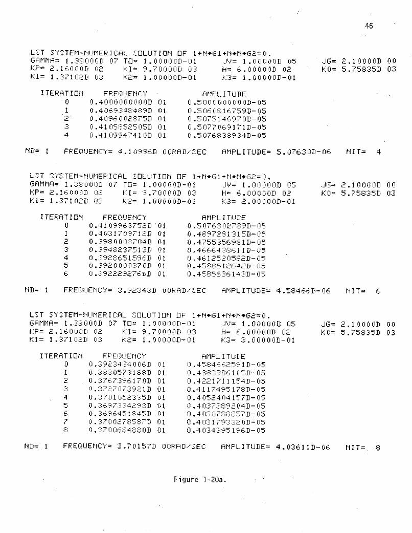
LST :S'TEM-NUMERICAL SOLUTION OF 1+N+1++NNiG2=0.GAMMA= 1.3:8:00lD 07 TO= 1. -= 10- V= 00000B 05 .JG= 2.10000D 00KP= 2.16000D 02 KI= 9.70000D 03 H= 6.o00o0D 02 KO= 5.75835D 03Kl= 1.371021 0:3 K= 1..00or'-01 K:3= 1.o000oD-01

ITERATION FREQUENCY AMPL ITUDE0 0.4000000000D 01 0.500nn000000no -051 0.4069348489 01 0.5060-16759D- 52 0.4096002875I 01 0.5075146970D-053 0.4105852505 01 0.5 077069171 D-054 0 .41 09947410 01 0.5076838934D- 05

ND= 1 FREQLUENCY= 4.10996D O00RAD/SEC AMPLITUDE= 5. 07630D-06 NIT= 4

LST :SYSTEM-NIUMERICAL :SOLUTION OF 1+N G1+N*N*G2=0.GAMMA= 1.3--000 07 TO= 1.0000rD-01 .JV= 1.00000D 05 .JG= 2.10000D 00KF'= 2.16000o 02 KI= 9.7000oD 0:3 H= 6.O00O0or' 02 KO= 5.75835D 03K1= 1.37102D 03 K2= 1.00000D-01 K3= 2.00000D-01

ITERATION FREQUENCY AMPLITUDE0 0.41 0996:3752DT 01 0.5076:302789D-051 0.4031709712D 01 0.48972813 15D-052 0.398: 0008' o704D 01 0.4755:356981D-053 0.39482:37513D 01 0.4666438611 D-054 0.:392651596D 01 0.461252058 2D-055 0.3920000370D 01 0.4588512642D-056 0.:9222976nD 01. 0.458:563614:3D-05

ND= I FREOUENC'Y= 3.92343D OOIRAD/SEC AMPLITUDE= 4.58466r-06 NIT= 6

LST SYSTEM-NUMERICAL SOLUTIDN OF I+N*G1+N*N.'*2=0.GIAMMA= 1.38-I000D 07 TO= 1 .O000D-01 .JV= 1.O0000 05 JG= 2.10000o 00KF'= 2.16000 02 KI= 9.70000 03 ' H= 6.00000 02 KO= 5.758351) 03Kl= 1.37102D 03 2= 1.0000OD-01 K3= :3 ,.O0000 -01

ITERATION FE'QU ENCY AMPL ITUDE0 0.392 4 4006D 01 0.4584662591D- 051 0.3830 573188D 01 0.4383986 1 05D-052 0.3767396170D 01 0.4221711154D-053 0.3727 0 73921I 01 0.4117495178D-054 0.3701052:335' 01 0.4052404157D-055 0. 369733 42931D 01 0.4037 -789204D-05

:6 0.369 64516 45j 01 0.40: 307888 57D-057 0.37002757D 01 0.4031793: 2 ID-05S 0.3700684880D: O 01 0.4 :'03439519 E 6D- 05

ND= 1 FREQUENCY= 3.70157D OORRD/zSEC AMPLITUDE= 4.03611D-06 NIT= 8

Figure 1-20a.

47

L:ST SYSTEM-NUMERICAFL ::OLUTION OF 1+N*G1+NN+*G3=0.GAMMA= 1.:3:8000:ID 07 TO= 1.00000D-01 J'v= 1.O0000 05 JG= 2.10000D 00

KFP= 2.1600D 2 KI= 9.70000Di 0:3 H= 6. 00 IoD 02 KO= 5.75835D 03Kl= 1.37102D 03 K2= 1.i000OO-01 K3= 4.00000D-01

I TERAT I ON FREOUE NCY AMPLITUDE0 0.370156717171 01 0.4 0361 0:8745D- 051 0.35828!6527D 01 0.3793426426D-052 0.3:496558: 168D 01 0. :3589545285D- 053 0.3435511973D 01 0 .3447780717D-054 0.33929303 01 0.3 3543 22:36D-055 0.33981930 57D 01 0.3352297996D-056 0.:33921473-26D 01 0.3:4063:1474D1-057 0.3395177657D 01 0.3339691379D-05

ND= 1 FREQLUENCY'= 3.3 :9539D O00RD:I/DSEC AMIPLITUDE= 3.33865D- 06 NIT= 7

LST SYSTEM-NUMERICAL SOLUTION OF I+N1*GI+N*GN2=0.GAMMrIA= 1.38000D 07 TO= 1i.0000OD-01 .JV= 1.00000 05 iG= 2.105001 O0KP= 2.16000D 02 KI= 9.70000D 03 H= 6.00000o 02 KO= 5.75835D 03K= 1.37102D 0:3 K2= 1.0000D-01 K:3= 5.O0000D-1

I TERAT ION FREQUENCY AMFL ITUDE0 0.33953- 263D' 01 0.3338654674D-051 0.32091 13-:520D 01 0.2976214976D-052 0.300 614935 01 0.2560 1 65D - 05

3 0. 115413321 0 - 0.8 497:375904D- 061 1.18541 00 -8. 4973:D-07

4 0.1 00000009D 01 0.9999999038r 005 0.100000000i i 01 0.1O 000000000D 01

ND= 1 FFREQUEINCY= 1.i00000ID OOFlRAD/S.":-.EC AMPLITUDE= 1l.O0000 00 N IT= 5

Figure 1-20b.

48

LST SYSTEM-NUMIER ICAL SOLUTION OF 1+N*I 1 +N*N*G2=0.GAMMA= 1.38000D 07 TO= 1.00000D-01 JV= 1.00000 D 05 .JG= 2.10000D 0 0KP= 2.16000D 02 KI= 9.70000D 0:3 H= 6.00OOD 02 KO= 5.75835D 03Kl= 1.37102 03: K2= 1.'0000D-01 K3= 1.0000-01

I TERAT I ON FREQUENCY AMPLITUDE0 0.1800000000D 0 01 0.6 O :00000000D-061 0.1829985273D 01 0.5796:322434D-062 0.18-:5465068:3D 01 0.5871916572D-063 . 18683794 0:D 01 0.593 048654D- ,4 0.187556.128D 01 0 .5963240748D-065 0 . 1: 87925743D 01 0 .59788647:35D-066 0.18799583027 01 0.5978609512D- 06

ND= 1 FREQUENC'Y= 1.88008D OORADSEC AMPLITUDE= 5.98399D-07 NIT= 6

LST SYSTEM-NUMERICAL SOLUTION OF 1+N*G1+N*N*G2=0.GAMMA= 1.3''8000'D 7 TO = 1.OD-01 JV= 1.00000D 05 .JG= 2.10000D 00KP= 2.16000D 02 KI= 9.7000D 03 H= 6.0OO0D 02 KO= 5.75835D 03Kl= 1.371023 03 K2= 1.00000D-01 K3= 2.0'0IOD-01

ITERATION FPEOUENCY AMPLITUDE0 0. 1880077917 01 0.59 3992937D- 061 0.1929412767 01 0.672, 2514:3D-062 0.196124166ED 01 0. 7186786352D- 063 0.1981174432D 01 0.745282...8246D-064 0. 1979638157 01 0.7715334579D- t065 0.1990078720D 01 0.77479 3764D- 066 0.1996130:59 01 0. 7774268:61D- 067 0. 1999099796 01 0.77376:81:85D-068 0.1999207661 01 0.7786887285D- 06

ND= 1 FREQUENCY= 1.99932D 00RAD'SECC AMPLITUDE= 7.78826D-07 NIT= 8

LST SYSTEM-NUMERICAL SOLUTION OF +N'1+N+C*.N*2=0.GAMMA= 1.3::3000' 07 TO V=1 .CD-01 J'= 1.00'000D 05 .JG= 2.10000 D 00KP= 2.16 00011 02 KI= 9.70000D 03 H= 6.0OOOD 02 KO= 5.75835D 03Kl= 1.37102D 03 K2= 1.00000D-01 K3= 3 .C CO 00D-01

ITERATION FREQUENCY AMPL ITUDE0 0.1 999323876 01 0.7788262524D-061 0. 206262759D 01 0.87343191 04D-062 0.21 '09'122091D 01 0. 9362249601D-063 0.21158 6739D 01 0. 1 0 07 9 2 0039D-054 0.21 2853221D 01 0.1009 006204D- 055 0.21456 65678: 01 i. 101600907D-056 0. 2152 49 ,86ED 01 0.10200' 51049D- '057 0.2155018071 D 01 0.102057588::4D- 05S 0.2155123139 01 0. 1 0214:38689 D-05

ND= 1 FREQUENC'Y= 2.155:34D OORASEC AMPLITUDE= 1 .02156D-06 NIT= 8

Figure 1-21a.

49

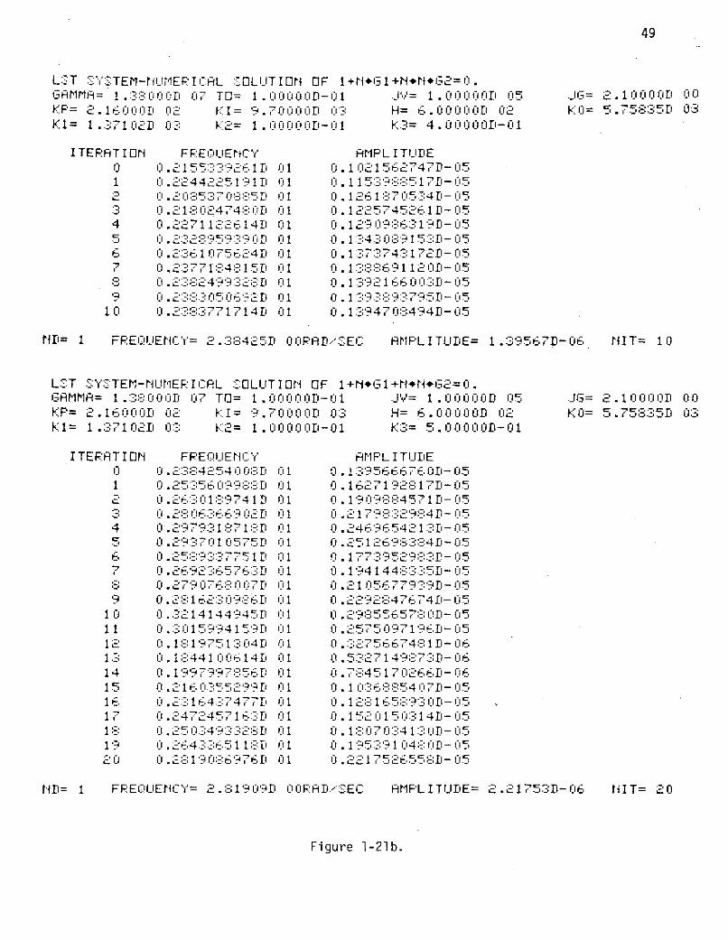
LST SYK:TEM-rNUMERICIL SOLUTIOrN OF 1+NG 1 +N*N*G2=0.GRMMA= 1.38000 07 TO= 1.00000D-01 JV= 1.00000 05 ._3G= 2.10000 00KF'= 2.160C' 012 KI= 9.7'000D 03 H= 6.0000D 02 KO= 5.758335D 03K1= 1.371021 03 K2= 1.0000D-01 K.3= 4.00000D-01

ITERATION FREOIUENCY AIMPLITUDE0 0.21553 9261D 01 0.1021562747D- 051 0.2244 225 191 01 0.1153988517 D- 052 0.2085 370885 01 0.1261 7 534D - 05 ,3 .2 1 8024 74: 80D 01 0.1225745261D-054 0.2271122614D 01 0.1290986319D-055 0 .2328959390D 01 0. 1 34308 915:: D- 056 0.2361075624 01 0.1:3 73743172fD-057 0.23771:4::15D 01 0.138869'-1120D-058 0.2 38249?932:D' 01 0.139 216 6. 003D- 059 0.2383050692D 01 0.1 393:893795D-05

10 0.2383::771714D 01 0.1:3947 08494D- 05

ND= 1 FREQIUENCY= 2.38425D OORAD/SEC AMPLITUDE= 1.39567D-06 NIT= 10

LST SYSTEM-NUMER I CAL SOLUTION OF 1+N*G1+N*N*G2=0.IGAMMR= 1.:38000D 07 TO= 1.00000D-01 JV= 1.0000D 105 JG= 2.10000D 00KP= 2.16000£ 02 KI= 9.70000D 0:3 H= 6.00000) 02 KO= 5.758351' 03Kl= 1.:37102£' 013 K2= i .00000D-01 K3= 5.00001:OD-01

ITERAT ION FREQUENCY AMPLITUDE0 0.23:84254008D 01 0.1:395666760D-051 0.25:356 09988: 01 0. 1627192817D-052 0.26:30189741 1D 01 0.190988:34571 D- 053 0.2:806366902D£ 01 0.2179832984D-054 0.297931871.D 01 0. 2469654213D -05

5 0.2937010575 01 0.2512698384D- 056 0 .2589337751 01 0 . 177395298:3£- 057 0.2692365763D 01 0.194144833:35D-058 0.2790768007D 01 0.21 056 77939D-059 0. 2816230986D 01 0. 229247674- 05

10 0.3214144945D 01 0 . 2955657 D-0511 0.3015994159 01 0 .2575097196D-0512 0.1197513041 01 0. 2756674- 1- 0613 0.1 441 00614 01 0. 27149 7:3D- 0614 0.1''997997856DI 01 0.7:845170266D-0615 0.2160355-.299D 01 0.1036:885407D-0516 0 .2 1i6437477£ 01 0 .12165893- D0517 0.2472457163D 01 0.1520150314D-0518::: 0.25 0349332:: D 01 0.18:07 '03413:D: £- 0519 0. 264336511 : 01 0.195391040£- 0520 0.28:190:36976D 01 0.2217526553D-05

ND= 1 FREQUENCY= 2.81909D OORAD/SEC AMPLITUDE= 2.217533-06 NIT= 20

Figure 1-21b.

50

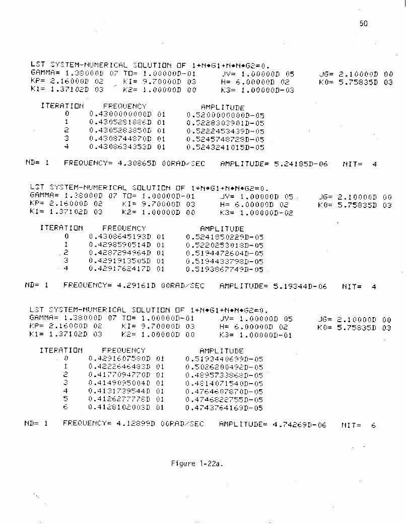
LST S'YSTEM-NUMERICAL 5CLUTIONr OF 1+N+*G1+N*,NG2=0.GAMMA= 1.3000 07 TO= 1.0:000iD-01 JV= 1.000D 05 JG= 2.10001 00KPF'= 2.16 000D 02 K I= 9.700 00D i 03 H= 6.0000 D 02 K O= 5.75835D 03Kl= 1.37102D 03 K2= 1.00000iD 00 K3= 1.0000D-03

I TERA T ION FREOUENCY AMPL I TUDE0 0.430 0000000 0 1 i0.52000 i 0000 D-051 .4305281886D 01 0 .52283039 01D- 052 0.4305283850 0. ' 5222453439D-05 5:3 0i.4:3087448:70D 01 . 524574728D- 054 0.4308634353D 01 0 .5243241015D-05

ND= 1 FREQUENCY= 4.308i65D OORAD.iSEC AMPLITUDE= 5.24185D-06 NIT= 4

LCT SYSTEM-NUIMERI:CAL SOLUTION OF 1+N*Gl1+N*N*G2=0.GAMMAF= 1.380:ii00Dr 07 TO= 1.0000ioD-01 JV= 1.00000D 05 JG= 2.10000D 00KP= 2.16000D 02r KI= 9.7ri0000D 03 H= I6.00OO'ID 02 KO= 5.75835D 03K1= 1.37102D 03 K2= 1.00000D 00 K3= 1.00000o-02

ITERATION FREQUENCY AMPLITUDE0 0.4:33645193D 01i 0 .524185229D- 051 0.4298590514D 01 0.5 220253018D- 05.2 0.4287294964D 01 0.5194472604D-053 0.42'9191:3505Di 01 0.51944:33798D- 054 0.4291762417D 01 0.5193867749D-05

ND= 1 FREQLIUENCY= 4.29161D O0RADI'SEC AMPLITUDE= 5.19344-06 NIT= 4

LST SYSTEM-NUMERICAL SOLUTION OF 1+N*6I1+N*N*G2=0.GAMMA= 1.3::8000:iD 07 TO= 1 .io riD-01 JV= 1. ]00D 05 JG= 2.10000D 00KF= 2.1600I0D 02 KI= 9.70000D 03 H= 6.'00000 02 KO= 5.75835D 03Kl= 1.37102r 0:3 K2= 1.0000D 00 K3= 1.i i ciOOI0D-01

ITERAT I ON FREQUENCY AMF'L I TUDE0 0.42916075803D 01 o0.519:3440699D-051 5 .4222646483D 01 0.5026200492D-052 0.4177094770D 01 .489. 573:68:D-053 0i.4149095004f 01 0 .48:1407154 D-054 0.4 1 1 7:39544D 0 1 0.47646 0 ' 787 D-055 0 .412627777 01 0.4746822755D-056 0.4128102003D 01 01 .474:3764169D-05

ND= 1 FREQIENCIY= 4.12899D OOFRAD/SEC FIMPLITUDE= 4.74269D-06 NIT= 6

Figure 1-22a.

51

LST SYSTEM-MUrMER ICIL SOLUTION OF I+N*G1+N*N+*2=0.GAMMFA= 1.38:000D 07 TO= 1.0000 OID-01 JV= 1.0000'D 05 ._JG= 2100001 00KP= 2.16000D 02 KI= 9.70000D 03 H= 6.000001 02 KO= 5.75835D 03K1= 1.371021) 03 K2= 1.00000D 00 K3= 2.000010D-Ol

ITERATION FRE!QUENCY AMPL ITUIDE0 0.4129866'01D 01 0.4742691103D:-051 0.4 0:8338::311) 01 0 .4534458733 D-052 0.3977078042D 01 0 .436916734 D-053 0.:3938140899D 01 0.4264565926D054 0.3913052885D: 01 0.4198877967D-055 0.3909417445D 01 0.41 34510 86D- 056 0.3908686.36,5D 01 0.4176817051D- 057 0.3910473948D 01 0.417557537 0D-05

ND= 1 FREQUENCY= 3.91085D 00RADF/SEC AMPLITUDE= 4.17559D-06 NIT= 7

LST :SYSTEM-NUMER ICAL SOLUT I ION OF 1+N*G1+N*NG2=0.GAMMA= 1.380001D 07 TO= 1.00000D-l01 .JV'= 1.00000D 05 JG= 2.100001 00KP= 2.16000D 02 KI= 9.70000D 0:3 H= 6.00000D 02 KO= 5.75835D 03Kl= 1.37102Di 03 K2= 1.O00000D 00 K3= 3.00000D-01

I TERATION FREQUENCY AMPLITUDE0 0.:391 085069:3D 01 0.4175586358 D- 051 0.37960230 :96D 01 0.:39267:34444D-052 0. 712 :8035 01 0:-3720541479 D- 053 0.,365-,41 73534D 01 0.3577665941D-05

4 0.36 1 '395577D 01 0.3485137376D- 055 0.36 19420497D 01 0.:34831883:: 29D-056 0.36114930 35D 01 0.: 46:3979466D - 057 0.361562674D 01 0. :346872725'-D- 058 0.3615619356 01 0. 3467415619D-05

ND= 1 FREQUENCY= 3.61565D OORAD/SEC AMPLITUDE= 3.46667D-06 NIT= 8

LST SYSTEM-NUMER I CAL SOLUT I ON OF 1+N G 1 +N*N.*G2= 0.GAMMA= 1.3:8000D 07 TO= 1.00'000D-1 JV= 1.00000D 05 JG= 2.10000D 00KF= 2.16000D 02 KI= 9.70000D 0:3 H= 6 . 000001' 02 KO= 5 .75:35D 03Kl= 1.:37102D 03 K2= 1.00000 oDr 0 3= 4.000001-01

I TERAT ION FREQUENCY AMPL I TUDE0 0.:615649056D 01 0.3466672496D-051 0.:34:34297949D 01 0.3093089012- 052 0.3240677649D 01 0.266998:0182D1- 053 0.1:8:0972125:8:D 01 -0.1572573 19:3D- 06

1 1 .0972D 00 -1.57257D- 07IHC900I EXECUTION TERMINATING DUE TO ERROR COUNT FOP ERROR NUMBER 261

Figure 1-2 -2b.

Figure 1-22b.

52

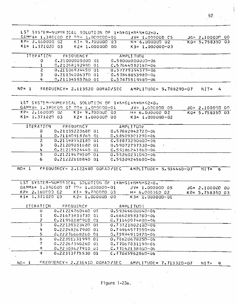
LST SYSTEM-NUPERICAL SOLUTION OF 1+N*GL+N*NG2=0.GAM4'A= 1.380COD 07 TOl= 1.OCOCOD-01 JV= 1.000000 C5 JG= 2.100000 00KP= 2.16000D 02 KI= 9.700000 03 H= 6.000000 02 KO= 5.758350 03Kl= 1.37102D 03 K2= 1.00000D 00 K3= 1.000000D-03

ITEP AT ION FFREOJENCY AMPLI TUOE0 0.21000000000 01 0.5800000000D-061 0.21058192980 01 0.57644082180-062 0.21106834450 01 0.57779394370-063 0.2113400637D 01 0.57848853980-064 0.2113458576D 01 0.57875519580-06

ND= 1 FREQUENCY= 2.113520 OORAD/SEC AMPLITUDE= 5.788290-07 NIT= 4

LST SYSTEM-NUMEPICAL SOLUTION OF 1+NGl+NN*G2=0.GAMMA= 1.380C00 C7 TO= 1.Orn0D0-01 JV= 1.000000D 05 JG= 2.100000 00KP= 2.160000 02 KI= 9.700000 03 H= 6.0U0000 02 KO= 5.75835D 03Kl= 1.371020 03 K2= 1.O0000D 00 K3= 1.000000D-02

ITERATICN FREOUFNCY AMPLITUDE0 0.21135223680 01 0.57882942720-061 0.2118091876D 01 0.5850930129D-062 0.2119895218D 01 C.5887325060D-063 0.2120905168D 01 0.5907279733D-064 0.21215524440 01 C.51186241860-065 0.21219679300 01 0.5926023104D-066 0.21222618840 01 0.5930924560D-06

ND= 1 FREQUENCY= 2.122480 00RAD/SEC AMPLITUOE= 5.934460-07 NIT= 6

LST SYSTEM-NUMR ICAL SOLUTION OF 1+NvGL+N*N*G2=0.GAMVA= 1.390000 07 TO= 1.000000-01 JV= 1.00000D 05 JG= 2.100000 00KP= 2.160000 C2 KI= 9.700000 03 H= 6.0000GD 02 KO= 5.758350 03Kl= 1.371020 03 K2= 1.000000 00 K3= 1.000000D-01

ITERATICN FPEQUENCY AMPLITUD-0 0.2122476046D 01 0.59344600040-061 0.21673833730 01 0.66628583780-062 0.2195828091D 01 C.71140074880-063 0.22128323420 01 0.73721802100-064 0.22248267900 01 0.74964577550-065 0.22276668260 01 0.75994910370-066 0.22301331990 01 0.78620678250-067 0.2226734026D 01 0.77067831190-068 0.2230362791D 01 C.7714213880D-069 0.22313775530 01 C.7708596286D-.06

ND= 1 rREOIJENCY= 2.231410 OORAD/SEC AMPLITUDE= 7.713320-07 NIT= 9

Figure 1-23a.

53

LST SYSTEM-NIJMc ICAL SOLUTION OF 1+NGl+NrN*Gr2=0.GAM M A= 1.38000n 07 TO= .000000D-01 JV = 1.000000 05 JG= 2.100000 00

KP= 2.160000 02 KI= 9.700000 03 H= 6.000000 02 KO= 5.758350 03

Kl= 1.371020 03 K2= 1.00000 CO K3= 2.00000D-01

ITERATICN FREQUENCY AMPLITUDE0 0.22314055190 01 0.7713323182D-061 0.2 2 9 189 699 5D 01 C.87037847240-06

2 0.2333268636D 01 C.9360260647D-063 0.23674924000 01 C.97474662960-064 0.23758376840 01 0.10015089090-055 0.2379792S870 01 0.10134590340-056 0.23822084950 01 0.1C216618780-057 0.2382672134D 01 0.1C26021014D-058 0.23844971350 01 0.10265748260-059 0.23847699599 01 0.1C279821240-05

10 0.2385228987D 01 0.10283023410-05

ND= 1 FREOUENCY= 2.38548D OORAD/SEC AMPLITUDE = 1.028880-06 NIT= 10

LST SYSTEM-NUMERICAL SOLUTICN OF 1+N*Gl+NN*G2=0.GAMMA= 1.380000 07 TO= 1.000000-01 JV= 1.000000 05 JG = 2.100000 00KP= 2.16000D C2 KI= 9.7(,0000 03 H= 6.00000D 02 KO= 5.75835D 03K1= 1.371020 03 K2= 1.000000 00 K3= 3.000000-01

ITERATICN FREQUENCY AMPLITUD-0 0.23854834610 01 0.1C28881516D-051 0.2467801350D 01 0.11650479630-052 0.253SE528850 01 0.1266348362D-053 0.25578450900 01 0.1292374398D-054 0.2577636773D 01 0.13442010290-055 0.2588264309D 01 0.1369898918D-056 0.25948114380 01 0.13843215460-057 0.25995488080 01 0.1395250181D-058 0.2602932943D 01 0.14027589710-059 0.2605653351D 01 0.14103999390-05

10 0.2605424268D 01 0.1425499818D-0511 0.26124580090 01 0.14290249370-0512 0.26151963730 01 0.14293534980-0513 0.26152382070 01 0.14301389780-05

ND= 1 FREQUENCY= 2.615340 OOPAO/SEC AMPLITUDE= 1.43025D-06 NIT= 13

Figure 1-23b.

54

LST SYSTEM-NtUMER ICAL SOLUTION OF I+N*Gl+N*N*G2=0.GAMMA= 1.330000 07 Tr= 1.000000-01 JV= 1.0000D 05 JG= 2.100000 OCKP = 2.160000 02 KI= 9.700000 03 H= 6.00O0000D 02 KO= 5.758350 O'K1= 1.371020 03 K2= 1.000000 UO K3= 4.000000-01

ITERATION FREQUENCY AMPLITUDE0 0.26153383290 01 0.1430252227D-051 0.27491451770 01 0.16576896760-052 0.271550C 8060 01 0.18331919630-053 0.28568670450 01 0.19921476640-054 0.30181244280 01 0.22431135990-055 0.32362731020 01 C.26300592738-056 0.29855021500 01 0.2252579941D-057 0.31768831180 01 0.2567539012D-058 0.19141123C90 01 0.4284134675D-079 0.20833868460 01 0.64302884600-06

10 0.2288243203D 01 0.9357461008D-0611 0.24575102290 01 0.11954391140-0512 0.25991500320 01 0.14282643080-0513 0.2719769617D 01 0.1635828728D-0514 0.282444339D 0 01 .120999738D-0515 0.29220335750 01 0.19938006230-0516 0.28804182890 01 0.2C716253490-0517 0.30153749000 01 0.22590807780-05

18 0.32966725560 01 0.27652305310-0519 0.3005244254D 01 0.22179562590-0520 0.32077926070 01 0.25743091210-05

ND= I FREQUENCY= 3.20779D OORAD/SEC AMPLITUDE= 2.57431D-06 NIT= 20

LST SYSTEM-NUMERICAL SOLUTION OF 1+N*Gl+N*N*G2=0.GAMMA= 1.38CCOD 07 Tl= 1.00o00n-01 JV= 1.00000D C5 JG= 2.100000 00KP= 2.160UO0 02 KI= 9.70000D 03 H= 6.000000 02 KO= 5.758350 03KI= 1.37102D 03 K2= 1.000000D 00 K3= 5.000000-01

ITERATI3N FREOIJENCY AMPLITUDE0 0.3207792607D 01 0.2 57430912 10-051 C.9630C656000 00 -0.18201961810-05

1 9.630070-01 -1.8202UD-06

IHC900L I XECUTION TEPRINATING DUE Tn ERPOR COUNT FOR FRROR NUMBER 261

Figure 1-23c.

55

LST SYSTEM-NUMERICAL SOLUTION OF 1+N+I1+N*N*G2=0.GAMMA= 1.38000D 07 TO= 1.00000-01 J'-= 1.00000D' 05 JG= 2.10000D 00KP= 2 .16000D 02 K I = 9.70000D 03 H= 6.0000D 02 KO= 5.75835 03Kl= 1.37102D 03 K2= 5.00000D 00 K3= 1.0000o-03

ITERATION FREQUENCY AML I TUDE0 0.4400000o000D 01 0.380000000oo-051 0.4362207906D 01 0.37:3862'1826DE.l- 052 0.4366626986D 01 0. 77 03966 09D- 053 0.4371378655D 01 0.379666476:3D- 054 0.4371379386D 01 0.379697102 D-05

ND= 1 FREQUENCY= 4.3713SD 00RAFD.SEC AMPLITUDE= 3.79739D-06 NIT= 4

LST SYSTEM-NUMERICAL SOLUTION OF 1+N*61+NN*G2=0.GAMMA= 1.38000 07 TO= 1.O0000D-01 J''= 1.00000 05 JG= 2.1C000F 00KP= 2. 16000D 02 K I = 9.70000 or 0:3 H= 6 . 00 o oD 02 KO= 5.758350 03KI= 1.37102D 0:3 K2= 5.00000D 00 K3= 1. 0000D-02

ITERATION FREQUENCY AMPL I TUDE0 0.4371 78655 01 0.:379739 n715D-051 0.4439449719D 01 0.3922771641D-052 0.43-944729:3D 01 0.3806676407D- 053 0.4 516 26143D 01 0. :3715020961 - 54 0.4308103:30 01 0.360061 8889D-055 0.426 02005:3 01 0.3670741887D-056 0.4328794391 01 0.36-432506 D- 057 0.432 1 3561S 01 0.36 125923 91D - 05

0.4327365248D 01 0.3646707945 D-059 0.4337145059 01 0. 94037842D-0 -

10 0 .4340696990 01 0. :371532488D- 0511 0.4340665599 01 0.3717126124D-05

ND= 1 FREQUENCY= 4.34039D OORAF'SEC AMPLITUDE= 3.71822D-06 NIT= 11

Figure 1-24a.

56

LST :S'TEM-NUMEFICAL SOLUTION OF 1+N*G1+N*N*G2=0.GAMMA= 1.2:8000nD 07 TO= 1.00000D-01 J''= 1.00000D 05 JG= 2.100001'l 00KP= 2.16000D 02 KI= 9.70000D 03 H= 6.00000' 02 KO= 5.75835D: 0:3

Kl= 1.37102DJ 03 K2= 5.1'.000 01' 0 K3= 1.100001D-01

ITERATIO N FREQUENCY iAMFL I TUDE0 0.4340393741D 01 0 .:3718223726D- 05I 0.419 00 991 01 0.35339199 D- 052 0.4044315491D 01 0 .2984572933D- OS053 0.:3747709579 01 0.2:300337882D-054 0.1 .884955 159D 01 0.256637093- 055 0.3894792652D 01 0 .258337 07284D-056 0. 3899572181 01 0.26620491 62D- 057 0.55020759 01 0.25323411 29D-058 0.37-2 1 5 2 7 7 1 0D 01 0.2238764 305D-059 0.38: 07352703D 01 0.2-3943221-05

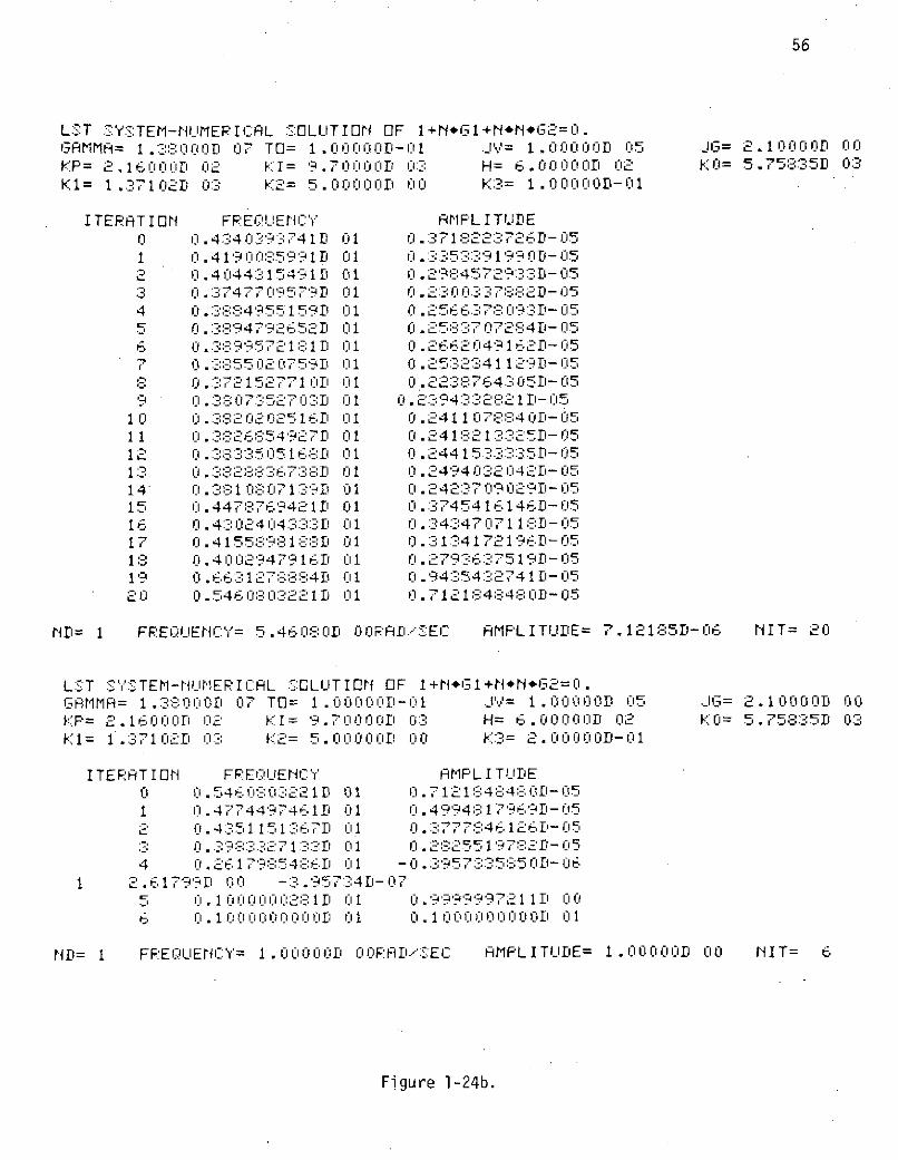
10 0.38202025 16 01 0.241 1 078 4D-0511 0. 3826854927D 01 0.2418213325D- 0512 0.3833505163 01 0.2441533335D-051:3 0.3828836738 01 0.249403 2 042- 0514 0.3810807139 01 0. 4 37 09029D-0515 01.4478769421 01 0.37454 16146D- 0516 0.4:30 2404333 01 0.343470711 D-0517 0.4155:898188 01 0.313417 2196D-05183 0.4'002947916 01 0.27926 ' 3" 7519D-0519 .6631278884D 01 0 .94354274 1 D-0520 0.5460803221 01 0. 712184:84 OD- 05

ND= 1 FREQUENCY= 5.46080D 00RAD/.'SEC AMPLITUDE= 7.12185D- 06 NIT= 20

LST SY'-STE-NUMERICAL SOLUTION OF 1+N*G +*N+*G2=0.GAMMA= 1.38000 07 TO= 1 . 000D-01 J~= 1.00 001 05 .JG= 2 . 10 0 00 00KP= 2.16C00D 02 KI= 9.70000D( 03: H= 6.000001 02 KO= 5.75835D 03K 1 = 1. 3710'2D 03 K2= 5..0D 00 K3= 2 .'0 'D-01

ITERATION FF :REQUENCY AMF'LITUDE0 0.5460803221D: 01 0.7121 -:848:34D-051 01 .4774497461 01 0 .499481 7969D- 052 .4351151 367D 01 0.377746126D- 05

S0.398:3-3271 :3:3D 01 0.28 2551 9782D- 054 0 . 26E17'9854:86D 01 -0.3957:3:35:35 o5- 06

1 2.61799D 00 -:3.95734D-075 0.1000000281D 1 0.99999'97211D 006 0.1000000000 i 0i i1 0.1000000000 01

ND= 1 FREQUENCY= 1.000001 O00RAD F.EC AMPLITUDE= 1.100000D 00 NIT= 6

Figure 1-24b.

57

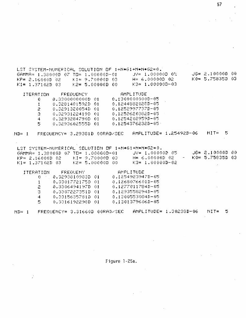
LST :S'Y:STEM-rUMERICAL SOLUTION OF 1+N*G1+N*N*G2=0.GAMMA= 1.:38000O 07 TO= 1.0000O-01 JV'= 1.OOOOD 0". JG= 2.10000D 00KF'= 2.16000D 02 KI= 9.70000o 0:3: H= 6.000D 02 KO= 5.75835D 03Kl= 1.37102D 03 K2= 5.00000D 00 K3= 1.0000OD-0:3

ITERAT ION FREQUiENCY AMPL I TLIDE0 0.:3:300000000D 0:1 0.1300 00000 -051 0.32: 148 1592D 1 0. 1244882028D-052 0.3291320054I 01 0.12529977:37D-053 0.:3293122419D 1 0.1252620382D-054 0.3293284790D 01 0.1254202959D-055 0.3293602555D 01 0.1254:376232D- 05

ND= 1 FREQUENiCY= 3.29:3:81 00RAD/:EC AMPLITUDE= 1.254921-06 NIT= 5

LST SYSTEM-NiUMERICAL SOLUTION OF I+~1G+N*NG2= 0.GAMMA= 1.3:80_:C00: 07 TO= 1.0000CD-1 .JV= 1.0000D 05 JG= 2.10000D 00KPF'= 2.16000D 02 KI= 9.0000D 0:3 H= 6. Ci000 D 02 - KO= 5.75835D 03Kl= 1.371I02D 3 K2= 5.0-0OD 00 K:3= 1.00lCOOD-02

I TERAT I ONF FREI_ UENI' AMPL I TULDE0 0.3293810983::D 01 0.125492:3947D-051 0. 330177 175D 01 0.1268076601D-052 0.3306494197D 01 0.1277011784D-053 0.3307227351D 01 0.129:3558294D-054 0. 3315 63 5781 0.1:0553 :34D-055 0.:331619229D 01 . 1301379606D-05

ND= 1 FREQUENCY= :3.31660Di OORAD/SEC AMPLITUIDE= 1.302:38D-06 NIT= 5

Figure 1-25a.

58

LST :S'S:TEM-NUIMERICAL SOLUTION OF 1+Ni*G 1+N*N*G2=0.GAMMA= 1 .38000D 07 TO= 1 .i01-01 V= 1 . 000001 05 .JG= 2.1000 D 00KP= 2.16000D 02 KI= 9.70000D 03 H= 6.O'OOOOD 02 KO= 5.758:35D 03Kl= 1.37102D 0:3 K2= 5.00000D 00 K3= 1.00000-01

ITERATION FREQUEN CY AMFPLITUDE0 0.3316597982D 01 0 . 130 2:379026D - 051 0.3413S:6922D 01 0.1504480:331D-052 0. 49713 166D 01 0.167520953::D-053 0.36509r83247D 01 0.186:3445424D-054 0.3825855:1D 01 0.2333538259D- 055 0.4025859796D 01 0.2869226076D-056 0.4: 0671996:3D 01 0.360095328D- 057 0.416:345E:4D 1 01 0.329:357101:3D-05: 0.4010876222D 01 0. 2903- 4972D-059 0. ::55 02:083028 01 0. 18: 74565879D- 05

10 0 .3642164:396D 01 0.2031512541D-0511 0 .3688151376I 01 0.2110027783:D-0512 0.3705009393D 01 0.2138959098D-0513 0.37116:39221D 01 0 .2090685945D- 0514 0.:3790756437 01 0.2319209448D-0515 0.3810400446 01 0.238560:39:34D-0516 0.3814455882 01 0.2511116680D-0517 0.3993908443D 01 0.2866222875D-0518 0.3631616890D 01 0.2051966841 D-0519 0.:3057705816D 01 0.2176188941D-0520 0I.3752088065 01 0.225:3631425D-05

N= 1 FREQUENCY= 3.75209D OORAD/SEC AMPLITUDE= 2.25363,06 NIT= 20

LST :SYSTEM-UMERICAL SOLUTION OF 1+N*61+N*N*G2=0.GAMMA= 1.:38:000D 07 TOD= 1.0000001-01 J'= 1.00000D 05 JG= 2.10000 00KF= 2.16000D 02 KI= 9.70000D 03 H= 6.00000D 02 KO= 5.75835 03

K1= 1.37102:i 03 K2= 5.00000r 00 K3= 2.00000D-01

I TERATI ON FREQUENCY AMPL ITUDE0 0.3:752088065D 01 0.2253631425D-051 0.42090561:32 01 0.3272927164D-052 0.38340 5192D 01 0.25605461:35 I- 053 0.538::060 8385D 01 0.61521 .3 8662D-05

4 0.4758738:637 01 0 .4 7 88:15:369 I-055 0 .43427 1489D 01 0.361723091- 05

6 0.3980004715D 01 0.2815716924D-057 0.2544538 760D 01 -0 .564:3857587D - 06

1 2 .54454D 00 -5.64386D-078 0.99999987711' 00 0.1000000125D 019 0.100000000D 01 0 .1000000000D 01

ND= I FREQLIENCY= 1.00000D OORAD/SEC AMPLITUDE= 1.00000D 00 NIT= 9

Figure 1-25b.

0.1

0.0 II

0.0010.00! 0.01 0.1 1.0 10.0

K 2

Figure 1-26. Region of self-sustained oscillations in the K2 - K3 plane for the two-axis LST system.

0

5 K2= 6.0SK 2 = 70 K = 0.001

K =0001 K 0.0K3 0.0

D 3 LUTIO

, K =0.2

2 =- K2 , 0.4K2=O.O

K3 = 0.0

o I I I I I I0 I 2 3 4 5 6

AMPLITUDE (xl(16 )

Figure 1-27. Region of possible solution points for the two-axis LST system.

61

REFERENCES

1. B. C. Kuo and G. Singh, Design of the Large Space Telescope System,Final Report, for NAS8-29853, Systems Research Laboratory, Champaign,Illinois, July 1, 1974.

2. B. C. Kuo and G. Singh, Continuous and Discrete Describing FunctionAnalysis of the LST System, Final Report, for NAS8-29853, SystemsResearch Laboratory, Champaign, Illinois, January 1, 1974.

62

2. Prediction by Numerical Methods of Self-Sustained Oscillations

in a Two-Axis Model of the Nonlinear Sampled-Data LST System

2-1. Introduction

It has been demonstrated in [2] that the stability equations as

a result of the describing function analysis may be solved by a

numerical-iterative technique. In Chapter 1, the numerical technique

is applied to the prediction of self-sustained oscillations in a two-

axis model of the nonlinear LST system with continuous-data. In this

chapter the same numerical technique will be extended to the prediction

of self-sustained oscillations in a two-axis model of the nonlinear

LST system with sampled-data.

In the two-axis model of the LST system, the system contains two

nonlinearities, and the general form of the stability equation in the

sampled-data case is

1 + GB(T,n)N(A,n,f) + GC(T,n)N2(A,n,f) = 0 (2-1)

where GB(T,n) and GC(T,n) are transfer functions which describe the

linear elements of the coupled systems, and N(A,n,P) represents the

discrete describing function of the CMG nonlinearity. The amplitude of

the sinusoidal signal at the input of the nonlinearities is denoted by

A; T is the sampling period in second, and n is the integer which relates

the period of the sustained oscillation to the sampling period; is the

phase angle of the input sinusoid. Therefore,

63

Tc = nT = period of sustained oscillation (2-2)

or

WC 2 = frequency of sustained oscillation in rad/sec (2-3)

2-2. The Sampled-Data Two-Axis LST System Model and Its Stability

Equation

Figure 2-1 illustrates the signal flow graph representation of

the sampled-data single-axis LST system. The nonlinear friction of

the CMG is modeled by the branch with the gain N, where strictly, N

denotes the discrete describing function N(A,n,f). The sample-and-hold

at the input of the nonlinearity is added for analytical purposes, so

that the overall system may be treated by the z-transform method.

Since the actual system does not have the sample-and-hold preceding N,

the system configuration of Fig. 2-1 should be considered as an approxi-

mation to the sampled-data single-axis LST system.

Figure 2-2 shows the two-axis model of the LST system, with the

coupling made at the output stages. The coupling coefficients K2 and

K3 may be varied for various degrees of coupling between the two single-

axis systems.

For the study of self-sustained oscillations, we set X, = X2 = 0.

From the signal flow graph of Fig. 2-2, the following cause-and-effect

relationships are written for the variables at the outputs of the four

samplers:

E*= -A*E* + A*N*X* + A2E2* - AN*X(2-4)1 1 1 3 1 2 - AN*X (2-)

E*= -A*E* + A*N** AE* - A*N*X* (2-5)2 1 2 3 2 + 2 1 4 .1

-I

Ks+KG3 (s) = Ps G(s) = K + K s3 1 K

G6(s) s G (s) K+ K11G 2 K D s + K

G7(S) =

1-eG (s) = 1 TsGho(S) 1 - Ts

ho s

Figure 2-1. The single-axis sampled-data LST system model.

65

-I

--3 6 H S.4 e

X, el T el* I/S-N

Gno X ) -K -K

-- K

ez T e

G4 (s) I / J (s5/Ks+K +K2)

Figure 2-2. The two-axis sampled-data LST system model.

-I

-K

Figure 2-2. The two-axis sampled-data LST system model.

66

X*= -B1N*X + B2E 1 (2-6)

X 2 = -B*N*X* + B2E2 (2-7)

where

GhoG1 G2G3G4G6HA1 (2-8)1 A

0

GhoG 1 G2 G3G4 G6HK2 AA2 = A = A1G4K2 (2-9)

A G 4 6 HA1 (2-10)3 A0

Gh GoG1G G6HK2 1A4 = = A3G4K2 (2-11)

0

B1 = sA (2-12)

GhoG2G3G6A 2B2 = sA = BG 2G3 (2-13)

A1 = 1 + G3G6 (2-14)

A 1 + 2G3 G6 K 2 2 2 2GG 2 G2 G 2 22 2K2

=1 - 2 4 3 6 2G3G GK 3462 (2-1 5)

2 3 6 2 2 2 22 = 1 + G3G6 - G3G6K2G4 - K2G4 (2-16)

In the last nine equations all functions are functions of s. The

sampled signal flow graph of the system is drawn in Fig. 2-3 using

Eqs. (2-4) through (2-7).

The determinant of the sampled signal flow graph is obtained from

Fig. 2-3 by use of Mason's gain formula. The expression is given in

terms of the z-transform functions:

-A4N

-A A2

A3 N

B -A4N

> E; > 2

A )Na Xi E2 B2

-A, -Bi

A g

Figure 2-3. Sampled signal flow graph of the two-axis sampled-data LST system.

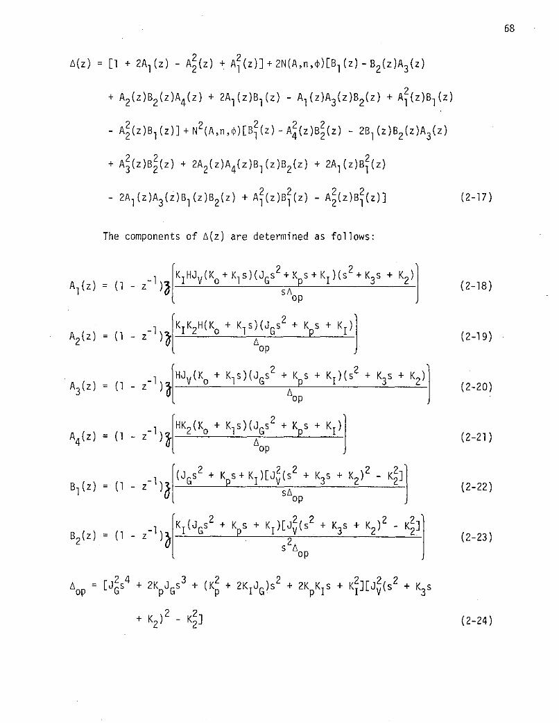
68

2 2A(z) : [I + 2Al(Z) - A 2 (z) + Al(z)] +2N(A,n, )[Bl(Z)- B2(z)A3(z)

+ A2 (z)B2 (z)A4 (z) + 2A1 (z)B1 (z) - A1(z)A3 (z)B2 (z) + A2(z)B1(z)

- A 2 (z)Bl (z )] + N2 (A ,n , )[B 2 (z )- A4 (z )B (z ) - 2Bl (z)B2 (z)A3 (z)

2 2 2

+ A3 (z)B 2 (z) + 2A2 (z)A4 (z)Bl(z)B2(z) + 2A1(Z)B1 (z)

2z 2(z) 2(z)B 2(z)- 2A1(z)A3(z)B1 (z)B2 (z) + A1(z)B1 (z) - A2 (z)B1 (z)] (2-17)

The components of A(z) are determined as follows:

1 KIHJV(Ko+ K S)(JGs2+ K s+K )(2+ K3s + K2)A1(z) = (1 - z- )po sa (2-18)

1 K K2H(K + Kls)(JGs 2 + Ks + KI)A2(z) = (1 - zY Ao (2-19)

AHJV(Ko + Ks)(J + KGS + Kps + Kl)(s 2 + K3s + K2 )jA3(z) = (- z ) (2-20)op

HK2(K o + K1S)(JGS2 + KpS + K)

A ) s= (2 z+ op

KI(JG s2 + Kp + Ki)[ 2(s2 + K3s + K2 2 - K2B2(z) = (I - zl 2A (2-23)

s op

Ap = [js4 + 2K J 3 + (Kp2 + 2K JG)S 2 + 2K Kls + K]2 J(s 2 + K3s

+ K2 )2 - K 2] (2-24)

69

The expressions for the discrete describing function of the CMG

nonlinearity, N(A,n,p), may be found in [2]. In the present case,

since the two axes are considered to be identical, and the couplings

are symmetric, it is assumed that the amplitudes of the input signals

at the two nonlinearities are identical.

The stability equation is obtained by setting A(z) of Eq. (2-17)

to zero. It is apparent that A(z) = 0 is of the form:

A(z) = 1 + GA(z) + GB(z)N(A,n,p) + GC(z)N2(A,n,p) = 0 (2-25)

which can be written as

1 + GB(T,n)N(A,n,f) + GC(T,n)N2(A,n,) = 0 (2-26)

by dividing both sides of the equation by 1 + GA(z), and setting

z = ej 27/n (2-27)

Equation (2-26) shows that in the sampled-data system, there are

four variable parameters in the stability equation in T, n, A, and p,

whereas in the continuous-data system there are only two variables in

A and w.

2-3. Exact Solution of the Stability Equation of the Two-Axis Sampled-

Data LST System by Numerical-Iterative Techniques

The numerical-iterative method described in Chapter 1 is now used

to solve the stability equation of the two-axis sampled-data LST system,

Eq. (2-26).

In Eq. (2-26) we define

70

GB(T,n) = GRI + jGI 1 (2-28)

GC(T,n) = GR2 + jGI2 (2-29)

N(A,n, ) = NRl + jNI1 (2-30)

N 2(A,n,p) = NR2 + jNI2 (2-31)

where GR, G G1 GR2, GI2, NR1I Nil, NR2 , and NI2 are all real quantities.

When Eqs. (2-28) through (2-31) are substituted into Eq. (2-26),

and after grouping the real and imaginary parts, we have,

A = AR + jAI = 0 (2-32)

where

AR = 1 + GR1NR1 - GIINII + GR2NR2 - GI2NI2 = 0 (2-33)

AI = GIINR1 + GR1NIl + GI2 NR2 + GR2NI2 = 0 (2-34)

These two expressions represent two equations in four variables

in A, T, , and n. It is necessary to assign values to two of these

variables and solve for the remaining two using the numerical-iterative

method. In general, it is practical to assign values to T and n, and

Eqs. (2-33) and (2-34) are solved to yield A and p. Alternatively, we

may assign values to n and p, and solve for A and T. The latter case

has been carried out in the current study.

As in Chapter 1, we define

x (2-35)A

71

RF = (2-36)

Then, Eqs. (2-33) and (2-34) can be written as

F(x) = 0 (2-37)

The Newton-type quadratically convergent numerical method described

in Chapter 1 can now be directly applied to this two-variable system.

The following system parameters are used:

TGFO = 0.1 ft-lb

H = 600 ft-lb-sec

JG = 2.1 ft-lb-sec 2

K = 5758.35

K1 = 1371.02

K = 216 ft-lb/rad/sec

KI = 9700 ft-lb/rad

J = 105 ft-lb-sec2

y = 1.38 x 107

Three sets of coefficients of coupling are used for this study:

(1) K2 = 0.1 K3 = 0.1

(2) K2 = 1.0 K3 = 0.1

(3) K2 = 5.0 K3 = 0.1

72

For each integral n, and a fixed value of 4, a solution of Eq. (2-37)

is attempted with an initial guess on T and A. A convergent solution for

T and A together with the assigned n and t describes a sustained oscillation

in the system. One of the characteristics of the numerical method is that

the solution depends on the initial conditions set by the analyst. As

shown in the earlier studies, it is quite possible that a system may have

a multiple number of solutions for the same set of n and p. An exhaustive

search can only be conducted by a systematic scan of all the possible

combinations of the initial values in the iterative process, unless one

has general information at the outset on the number and the proximity of

the solutions.

Figure 2-4 shows the plots of the two solutions of T versus A for

K2 = K3 = 0.1, and for relative large values of n. The results are shown

only for ' = 00. When all the values of p are used, the solutions of T

and A trace out a loop in the T versus A domain. For large values of n,

these loops are very small, as the solutions are relatively insensitive

to n. As n decreases, these loops become more pronounced, as indicated

in Fig. 2-5. As n decreases, one of the solutions disappears, as the

amplitude of A becomes exceedingly small.

Figure 2-6 gives the computer results for K2 = K3 = 0.1 that

correspond to one set of solutions for # = 00. Figure 2-7 tabulates the

other set of results for K2 = K3 = 0.1 with p = 00. Figure 2-8 gives the

tabulations of results for K2 = K3 = 0.1, n = 4, and variable .

Figures 2-9 and 2-10 give the results with K2 = 1.0 and K3 = 0.1.

Figure 2-11 shows the solutions for K2 = 5.0 and K3 = 0.1 with = 00.

In this case, the amplitude of oscillation decreases as n decreases, so

that there is less chance for the low-frequency oscillations to occur.

73

The results indicate that harder coupling (larger values of K2 and K3)

tends to reduce the chance of self-sustained oscillations.

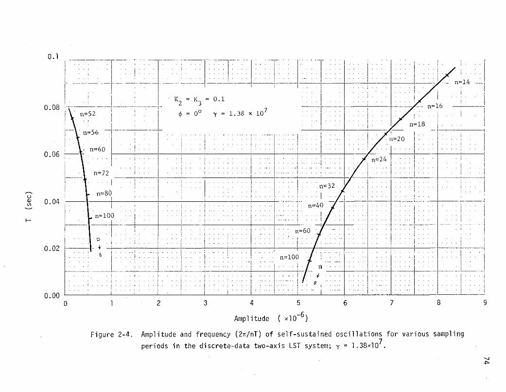
0.1

• _ L --.- - n=14

SK = 0.10.082 3 n160.08 52 00 y =1.38 x 107 T I

n=18

I a=20i. i . .. . . .. . . . .... ......... i . .. .

n=60 i ........0.06

n=72..................

n=32 . .. . ..n=80 . ... .

0.040.0 .. . .. i ....... i . .. i .............. .I . n=40... .... .. . .....

n=100

.- . . .. n= 6 0

0.02n=100

- '- -. -. . . .i .. ... ....

....i.. -S. . . . . . .... i .. ..

.-:... -....- _-._ ._._._. . . - -.- . . . . . ..--.-- ......0.00

0 1 2 3 4 5 6 7 8 9

Amplitude ( x10 - 6)

Figure 2-4. Amplitude and frequency (2i/nT) of self-sustained oscillations for various sampling

periods in the discrete-data two-axis LST system; y = 1.38xl07

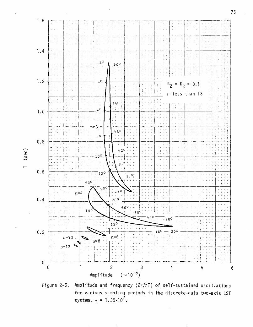
75

1.6

.. . . .... . .. .. . _ ... _ _ _ i_:.

. . . . . . . . . .

1.4. . . . . . . . . ..

20 060

~~t~ .... .......................

1.2 40. .K 2 K 3 0 .1

= - .. . n less than 13

540

1.0 60

480

1.0 . .__ . . . .

n=3 - __

0.8

420-100.1 -- I- -t \\2...... . . . . . . . .

360

0.6 120300V 900

0.4 700

600100 500

7 _ -L: . 300

120

0.2 160 - 200

n= 10 n=6n= 8

n=12

0

-o1 .1 I

0 1 2 3 4 5 6

Amplitude ( x 10-5)

Figure 2-5. Amplitude and frequency (2/nT) of self-sustained oscillations

for various sampling periods in the discrete-data two-axis LST

system; y = 1.38x107

76

LST SYSTEM-NUMEPICAL SOLUTION OF DISCRETE DESCRIBING FUNCTIONTWiO A:XIS-EQUIL AMPLITUDE CAS:-E, K2= 1.000D-01, K3= 1.000D-01GAMMA= 1.3.-000D 07 N= 100 PHI= 0.0

ITERATION :&AMIPLING PERIDD MPLITUDE0 0.:320000000D-01 0.6000000000D-061 0.3342229250D-01 0.59506798?07D-062 0.335978602311-01 0.5747976449'D-063 0.3366351585D- 01 0.566821 0713D-064 0.3369566512D- 01 0.5625329043D- 065 0.3369537215D-01 0.5627405691D-066 0.3369532634D-01 0.5435030290D-067 0.3364046622D-01 0.5571699439D-068 0 .:3367687123D-01 0 .5598125454D-069 0.3369855892D- 01 0 .56098 05886D- 06

10 0.3366940604D-01 0.562942754 OD- 0611 0.3:369303223D-01 0 .5630963918D-06

ND= I SAMPLING PERIOD= 3.36972D-02EC AMPLITUDE= 5.633421-07 NT=11

LST SYSTEM-NUMERICAL SOLUTIOI OF DISCRETE DESCRIBING FUNCTIONTWO A:IS-EQUAL AMFLITUDE CASE, K2= 1.0001D-01, K3= 1.000D-01GAMMA= 1.:::3:00D 07 N= 96 PHI= 0.0

ITERATION S-:AMPL ING PERIOD AMPL I TUDE0 0.3369720849101 0.5633423550 D- 061 0.34742"153SD-01 0.5443359999D-062 0 .3502:3754021D-01 0. 54 0937221- 063 0.35115121951-01 0.5512909117D-064 0.3515743:63- 01 0 . 553 60:;'799D-

065 0.3518081455D-01 0. 5546943617D- 066 0.3515967466D- 01 0. 55629'91 : 73D- 067 0.3518635462D-01 0.5566505449D- 06

ND= 1 SAMPLING PERIODD= 3.51849D-02SEC AMPLITUDE= 5.56679D-07 NT= 7

LST SYSTEM-NUMERICAL SOLUTION OF DISCRETE DESCRIBING FUNCTIONTWO AX IS-EQULIL AMPFLITLUDE CASE, K2= 1. 001- 0o1, K3= 1.00011-01GARIMA= 1.;30001D 07 N= 92 PHI= 0.0

ITERATION SAtIPL ING PERIOD AMPLITIIDE0 0.3516492122D-01 0.556679 0331D- 061 0.36:3263:378 0 D-01 0 .5664:24-7D- 062 0.366332901 6D- 01 0.5.393 70557;D - 063 0.3673534759D-01 0.543554356D-064 0.3678294190 D-01 0.5458594565D- 065 0.368 0:-7407D- 01 0.5469'41265::D- 066 0.3675900402D- 01 0.5494 0i 39::: :4D- 067 0. 3679886044D-01 I0.5492251 8 20D-06S 0.3680191726D-01 0 .5613414977D- 069 0.368661866D-01 0.55061744 07D-06

10 0.36E:451363-:D-01 0 5495252589'D- 0611 0.3683223886D-01 054'91315696D-0612 0. .698W''-.436993D- 01 0. 5-:462546:9- D- 0613 0.369154:345:D- 1 0. 537:99:2242D- 0614 0.36846532330-01 0.5439682800D- 0615 0 .36727252 04D-01 0.5512047322fD-06

ND= 1 SAMPLING PERIOD= 3.67273D-02SEC AMPLITUDE= 5.51205D-07 NT=15

Figure 2-6a.

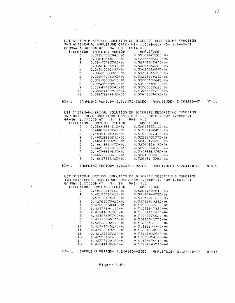
77

LST SYSTEM-NUMEPICAL :OLUTION OF DISCPETE DESCRIBING FUNCTIONTWO AXIS-EQUAL AMPLITUDE CASE, K2= 1.000D-01, K3= 1.00D-01GAMMA= 1.38000F 07 1N= S8 PHI= 0.0

ITERATION SAMPLING: PERIOD AMPLITUDE0 0.3672725204f-01 0.5512047:3-22D-06

1 0 . 3': 04951071 D 7-0 0. 5276 558662,- 1:162 0.3:-:40576574D-01 0 .529 9754747l- 063 0.3852469444D-01 0.5"3394 05723D- 064 0 .3858: 000219D- 01- 0 .53E.2532059D- 065 0 860782- 01 0.5:37:34. 15:-:9- 066 0 .388 09 0763D-01 0.5325967023D-067 0 . 3:E: 688 69: 63 D - 01 0. 5 7:?7 1 :3836411- 068 0.38 .625':289 OD - 01 0. 54 , 0775 0:67 D- 069 0.3 64.465::4 D- 01 0.5:3766687.62D1-06

10 0.386544397D-01 0. 5369724701-0611 0.3865827663D-01 0. 5367328089D-06

ND= 1 SAMPLING PERIOD= 3.86637D-02SEC AMPLITUDE= 5.36429D-07 NT=11

LST SYSTEM-NUMERICAL SOLUTION OF DISCRETE DESCRIEIr4G FUNCTIONTWO AXI:S-EIQUAL AMFLITUDE C:.ASE, K2= 1.0001-01, K:= 1.00OD-01GAMMA= 1.:38000 07 N= 84 PHI= 0.0

ITERATION SAMPLING PERIOD HMPLITUDE0 0. :3866 :66421 D- 01 .53 64285:-::8 1 D- 06,1 0.4 0023:64976D- 01 0.5 15 0~8;49745D- 062 0 .40:91001:341D-01 0.51 ': 0707747 - 063 0.405222392011-01 0.522109257- 064 0.405::,49 0375- ' 01 0. 524:717423D- 065 0.406 16 0445D- 01 0. 525408 : 19D- 066 0 .4071 0 42 31 D- 011 0. 52::9274439D- 067 0 .4 05966302 rSD- 0 1 0 . 5:: 5 992476D- 068 0 .4 063733 61 D- 01 0. 5264:-: 03961 D- 069 0.40637:3254D-01 0.5264214375D-06

ND= 1 SAMPLING PERIOD= 4.06373D-02SEC AMPLITUE= 5.26414D-07 NT= 9

LST SYSTEM-NUMERICAL S OLUTION OF I::CR:ETE DESC:IEINGB FUNCTIONTWO ANIS-EQUAL AMPLITUDE CA:SE. K2= 1.00D-01, K3= 1.0001-01GAMMA= 1.3:::00, 07 N= :0 PHI= 0.0

ITERATION AMFPLINGG PEPIOD AMPL ITUDE0 0 .4 06:373141 8D- 01 0.526414::39 04D- 06.1 0. 4219 79242D- 01 0. 5014704472D- 062 0 .4 26134951 : 8D-11 0 .50:3:542111l1 - 06.3 0 .4 276607502D- 01 0.507:31 a 0192:31-064 0 4 2 8:: :' 904 D - 01 0.5 , 0936:-9 22 7D - 0 E65 0. 42::770411 -01 0.510:29174:D-6 0.4 29416 8292D - 01 0 .5097411227D-067 0. 4 2957:9576-01 a .50 84227662D-068 0.4 29959951 OD-01 0.5 061 52377D-06

9 0 .42 23324 1 D- 1 I .512 056117D-0.1 0 0.4 L '7452? 01 0.51 :1564 094 D- 0611 0.429723-49'2 O- 01 0.5 .: 0:6490D - 0612 0.4212:5522-01 0.5:31 05 0:326D- 61:3 0 .425904 6767D-01 0 .518639:634 6412 D- 0614 0. 427725:391 ::D- 01 0 .5147 065691 I- 06.15 0 .4284118828D-01 0 .513 741 4959D- 06

ND= 1 SAMPLING PEPIOD= 4.28412D-02SEC AMPLITUDE= 5.13741F-07 NT=15

Figure 2-6b.

78

LST SYSTEM-NUMEPI CAL SOLUTION OF DISCRETE DESCRIBINiG FUNCTIONTWO AX.IS-ElQUAL AMPLITUDE CASE, A I2= 1.000D-01, K13= 1.0001D-01GAMMA= 1.3_000:O 07 1= 76 PHI= 0.0

ITERAT ION : AMPL ING PEPIOD AMPLITUDEO 0 .4284 11 8:.2:D- 01 0 .513 7414'959D- C061 0.446411 167D -1 0.4841942659D-062 0.4 51340469 -1 4 - 1 0. 4:_:50:0623D- 063 0.453145695:3D- 01 0.4 :32507D-064 54 .4009726E9D- 1 0.490;(2121 17:3D- 065 0.4544690240 D- 1 0.491 '105615 02D- 066 0.455 01585751- 0 1 0 .490: 0:3182 OD- 067 0.4550362.167D-01 0.49061 0:5:0 D- 06

ND= 1 SAMPLING PERIOD= 4.55056D-O2SEC AMPLITUDE= 4.90508D-07 NT= 7

LST SYSTEM-NUMEP ICAL SOLUTION OF DI:C.:CRETE DES:CRIBING FUNCTIONTWO AX:IS-EQUArL AMPLITUDE CAS-E, K2= 1. 000D-01 , K:3== 1.00C0D-01GAMMA= 1. :8:00D 07 N= 7.2 PHI= 0.i0

ITERAT ION : SAMPLIN'G PEPIOD AMPL I TUDE0 0. 45505647E:T:-D- 01 0. 4905 0772E 2D- 061 0 .474S492582D - 01 0.46 02676 0i60D- 062 0.4S0:32707:35- 01 0.46110528328D-063 0.4:824690167D- II 0 .46:3922.:444 D- C04 0.48:35 1 5:5:44 D-01 0. 465427910 2D- 065 0 .4 84071 00 2:-:D- 01 0 . 4661 C0 9461D- E066 0.445::6 0271'D- 1 0 .46601I 2E6242D- C067 0.484591382.23D-1 0.4659959617D-06

ND= 1 ':AMPLING PERIOD= 4.84594D-02SEC AMPLITUDE= 4.659:83D-07 NT= 7

LST SY:TEM-IUME I C:L ':OLUiTION OF DIS...R:ETE DE: CR I lING Fl-UNCT IONTWO AXIs I:-EQUAL AMPLITUDE CAS:IE, :K2= 1.00(oD-Ol1, K3= 1.O00CI'-01GAMIA= 1.:38000 07 N= 6: PHI= 0.0

ITERATION .AM'PL I NG PERIOD MF PLI TUDE0 0.48459423:-32 :- C01 0 .4659: ::321 941- 061 0.5077128819D- 01 0 .430554122CD-062 0 .5141496277D- h 1 0 .4 300':3 16467D- 06

3 0.51676 971 5D-- 01 0.4:31-96127:33- 064 0.51 0659:':'395D- l 1 0.4I 4:329 62 82:3:iD-065 0 .518751991 CD-O 01 C . 43:3733 30:--D- 066 0.51927923:3j1- 01 0.43:3355 569:D- I067 0.519279477'D-01 0.43:3:3E:8 1285D- 06

ND= 1 SAMPLING PERID= 5.A19:320D-022 EC AMPLITUDE= 4.:3332.-I-07 NT= 7

LST SYSTEM-NUMERICAL C-OLUTION OF DISCRETE DESCRIEING FUNCTIONITWIO AAXIS-EQUAL AMPLITUDE C AE, K.2= 1.00 ID-01, K3= 1.000D-01GAMMA= 1 .:38:I000D N= 64 PHI= C0.0

I TERAT ION SAMPL I rG PERIOD AMPLI TUDE0 0.5192797142D-01 - 0.4-::::858D- 01 0 .5467724495D-l01 0.39106 .l90'- 062 0.5544071603D-01 0. : -38'9:: 0: D- 063 0.5576780C112D- 01 0.3:65 0195D-4 0.559:32:3721 D-1 0.3:-:' 934 3046D- 065 0.5601946040D-01 0.3 .- :"-'99 6 S 4 21 7D- i066 0.5607441769D- C1 0 389989926 D-06

ND= 1 SAMPLING PERIOD= 5.60744D-02.EC AMPLITUDE= 3.90010D-07 NT= 6

Figure 2-6c.

79

LST SY$TEM-NUMERICAL SOLUTION OF DISCRETE DESCRIEING FUNCTIONTWO AXIS-EGUAL AMPLITUDE CA::E, K2= 1.000D-01, K3= 1.000-01GAMMA= I.:3800D 07 = 60 PHI= 0.0

ITERATION SAMPL ING PERIOD MPIFL ITUDE0 0.56074407241-01 0 .-:900104301D-061 0. 5943855184D- 01 0. 77:2,:4 D-062 0.603435799D-01 0.334C925505D-063 0.6075649615D-01 0.3: 32972694D-0-4 0 .60968:0899-01 0.3326451744D-065 0.6108143602D-01 0.13E17 4347D-0661 . 1 1399 6 02D- 1 .::3 1 3 1 C 1:3l-7 0.611399-:4 77D-01 0 .3289:::485 0- 068 0.61091716D- 1 0.:21 :56964D- 069 0..611 0 .3:342-1 442 5205D- 06

10 0.611:36 0'.4650-01 .:337713726D- 06I 1 0.61201:62 5D- 1 0. :3135 4294- 0612 0 . 6120'97519D- 101 0 .:0 16 222 '6D- 0613 0.61213 :374:36D- 0.3 2 97E 77155IT- 0614 0.61218116191-01 0.3295921224D-06

N1D= I '.AMPLING PERIOD= 6.12248D-02::EC AMPLITUDE= 3.29351-07 NT=14

LST S::YTEM-N'IMERICAL :OLU TION OF D ISrC:ETE DESCRI :ING FUNCTIONTWO AXI -EIUL tMPLITUDE CA.E, K2= 1. 000D-01, K3= 1.0001,-01GAMMA= 1.3:-:liOD 07 N= 56 F'HI= 0.0

ITERATION SAMPLIN G PERIOD AMPLITUDE0 0.6122479469D-01 0. 329: 50' 78D- 06.1 0 .654:33017611-01 0. 3 C 5775. , -1:12 0.6645173242D-01 0.26 :25 2 D-063 0. 6695797940 - 01 0.25c:9494244D- 064 0.6722604406-01 0.2 574:--,74605D- 05 0 . 67:37019::4: Dl- 01 0 .i:'564 : 9 75951D1- 06 0.674 3:6'90::-01 0. 2562: 79: ,06D- 0 67 0. 67439:-::-32S47D - 01 0.2557157062D- 068 0.6744 0923-88D- 01 0. 2559094333D-06

ND= 1 SAMPLING PEPIOD= 6.74417D-2SEC AMPLITUDE= 2.558:43D-07 NT= 8

LST SY:STEM-NUlMEPICAL S:OLUTION OF DISCPETE DESCRIEIING FUNCTIONTWO AXI-EQ'UL AF'PLITUDE CA :E, K2= 1.000D1--01, K3= 1. 000D-01GAMMA= 1 .3:8000 07 N= 52 PF'HI= 0.0

ITERATION :SAMF'LI NG PERIOD AMPL I TUDE0 0.6744166977D-0 1 0.255::430579D- 061 0.732:-:5077 27D-01 0. 15921660051F-062 0.751 -.299- - 0 1 0 :-.1 1037:6352D- 063 0.754419700D, 1 0.1414855224D-064 0.7548"8:93 1 =7D-.01 0. 1539:3:811 11D-065 0 .754 0 :-:72::4D- : 1 0. 1577965747D-066 0 . 753405 32- D-0 1 0. 1600971463 D- 067 0.7534675:54D-01 15:911 :3:4 D- 068 0.7656361713D-01 .10 522636:39D-069 0.7609634676D- 01 0.12975:3781D-06

10 0.75726425641-01 0 144: 1269- 0611 0.7551:359241 D-01 0. 15 14975:3D-0E.12 0 .754161 :3162D1-01 0.1 57: 5:3:3::, D- E0613 0. 755:5 54 D- 01 0. 159700- C D99:i- 0614 0 .7537:34.3091D-01 .1579 7 7493D- 0615 0 .753:306135- 01 0. 16000554 09D- 06

ND= 1 SAMPLING PERIOD= 7.53309D-025EC AMPLITUDE= 1.60006D-07 NT=15

Figure 2-6d.

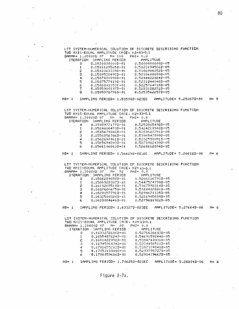
80

LST SYSTEM-NUMERICAL SOLUTION OF DISCRETE DESCRIBING FUNCTIONTWO AXIS-EQUAL AMPLITUDE CASE, K2=K~3=0.1GAMMA= 1.38:3000 07 N= 100 PHI= 0.0

ITERATION SAMPLING PERIOD AMPLITUDE0 0.15300000001-01 0.5000000000D-051 0.1513129565D-01 0.5123194566D-052 0. 1512363339D-01 0.518698252D-053 0. 150953:-49-D-01 0.52186 08:3 09D- 054 0. 150748'099:3D-01 0.5240422024D-055 0.1507577419D-01 0.5231844048D-056 0 .15 0453D- 01 0.5225764830 D-057 0. 1505980197D-01 0.5253128272D-058 0.1505978776D-01 0.5253562257D-05

ND= 1 SAMPLING PERIOD= 1.5059SfD-O2SEC AMPLITUDE= 5.25387D-06 N= 8

LST SYSTEM-NUMEPICAL SOLUTION OF DISCRETE DESCRIBING FUNCTIONTWO AXIS-EQUAL AMPLITUDE CASE, K-=K3=0.1GAMMA= 1.30-00D 07 N= 96 PHI= 0.0

ITERATION SAMPLING PERIOD AMPLITUDE0 0.1505977177D-01 0.5253865498D- 051 0. 152468..6473ED-01 0.542421 094D-052 0. 1545679 04:D- 01 0.5:35 068:7791 -053 0.1556856306D-01 0.5:306547099D-054 0.1562697461 D- 01 0.52-2550091 D- 055 0. 1565694849D-01 0.5270912439D-056 0.1566106363D-01 0.5268612074D-05

ND= 1 SAMPLING PERIOD= 1.56629D-02SEC AMPLITUDE= 5.26612D-06 N= 6

LST SYSTEM-NUMERICAL SOLUTION OF DISCRETE DESCRIBING FUNCTIONTWO AXIS-EQUAL AMPLITUDE CASE, K2= K3=0.1GAMMA= 1.38000D 07 N= 92 PHI= 0.0

ITERATION SAMPLING PERIOD AMPLITUDE0 0.1566289::353D- 01 0.526611679:::D-051 0.15869283 071D- 01 0.5447574799D-052 0.1610269510D-01 0.5367998314D-053 0.1622636675D-01 0.532 04 07881 D-054 0.1629157791D-01 0.5294671135D-055 0.1632500326D- 01 0.52:3190568 0D-056 0.1633084641D-01 0 .5279681922D- 05

ND= I SAMPLING PERIOD= 1.63327D-02SEC AMPLITUDE= 5.27664D-06 N= 6

LST SYSTEM-NUMERICAL SOLUTION OF DISCRETE DESCRIBING FUNCTIONTWO AXIS-EQUAL AMPLITUDE CA:-E, K2= K3=0.1GAMMA= 1.38000D 07 N= 3- PHI= 0.0

ITERATION SAMPLING PERIOD AMPLITUDE0 0.163::2726061D-01 0. 52766:3663:3D- 051 0. 1655487224D-0 1 0. 5469159244D-052 0.1631022992D-01 0. 5:3:474:39 31D- 053 0.169459 6034D-01 0.5334456511D-054 0. 1701655283D-01 0. 53 0774841D-055 0.1705310040D-01 0.5293798727D-056 0.1706059616D-01 0.5291479667D-05

ND= 1 SAMPLING PERIOD= 1.70625D-02SEC AMPLITUDE= 5.28804D-06 N= 6

Figure 2-7a.

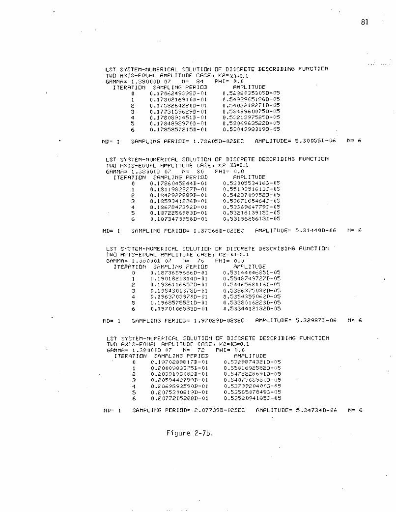
81

LST SYSTEM-NUMERICAL SOLUTION OF DISCRETE DESCRIBING FUNCTION

TWO AXIS-EQUAL AMPLITUDE CASE, K2=K3=0.1GAMMA= 1.3:000D 07 N= 8:4 PHI= 0.0

ITERATION SAMPLING PERIOD AMPLITUDE0 0. 170 624939:::D- 01 0.52 880: 353 05D-051 0. 1730216910D-01 0.5492965186D-052 0.175826422 0D- 01 0 .5403218271D-053 0.1773159629D-01 0.5349960075D-054 0.1780891451D-01 0.53 21397585D-055 0.17:489:8970D-01 0 .53 06Z963522D- 056 0.1785857215D-01 0.5304398319D-05

ND= 1 SAMPLING PERIOD= 1.786E05D-O2SEC AMPLITUDE= 5.30055D-06 N= 6

LST SYSTEM-NUMERICAL SOLUTION OF DISCRETE DESCRIBING FUNCTIONTWJO AXIS-EQUAL AMPLITUDE CASE, K.2==K3=0.1GAMMA= I .38000D 07 N= :0 PHI= 0.0

ITERATION SAMPLING PERIOD AMFLITUDES 0.1736045::441-01 0 300553416D-051 0.1 119:8E2227'D- 01 0.55 1's315 1E 13D- 052 0. 184292288:D-01 0.54237 I '952D-053 0.1859341236D-I 1 .5 3 .7165464D-054 0.1867847392'D- 01 053364779"D-5 0.18722569 3D - 01 0. 532161:3915D- 056 0.1873473958D-01 0.5318625613D- 05

ND= 1 SAMPLING PERIOD= 1.87366D-02SEC AMPLITUDE= 5.31440D-06 N= 6

LST SYSTEM-NUMERICAL SOLUTION OF DISCRETE DESCRIBING FUNCTIONTlWO AXIS-EQUAL AMPLITUDE CASE, K .2=K3=0.1GAMMA= 1.38000D 07 N= 76 PHI= 0.0

ITERATION SAMPLING PERIOD AMPL I TUDE0 0 .1 7:36,5'?666D-01 0 .5- 3144 146:385D- 051 0.1901820 14D-01 0.554. 749727D-052 0.19:36116657D-1 0.544656S81 16D-053 0. 195400-:7:3D-01 0.5 38 r-: 75032D-054 0.1963703870D-01 0 .5354355 0D- 055 0 . 1968D5755-21D- 01 0.5330162:28D-056 0.1970106583D-01 0.5334412132D-05

ND= 1 SAMPLING PERIOD= 1.97029D-2SEC AMPLITUDE= 5.32987D-06 N= 6

LST SYSTEM-NUMERICAL SOLUTION OF DISCRETE DESCRIBING FUNCTIONTWO AXIS-EQUAL AM'PLITUDE CASE, K2=K3=0.1GAMMA= 1.3::000D 07 N= 72 PHI= 0.0

ITERATION SAMPLING PERIOD AMPLITUDE0 0. 197028:39:1 7D- 01 0. .532974321 D- 051 0 .20009:3:-: 75D- 01 0 .55816: .925:D 2D- 1:152 0 . 20:3919 2- 01 0.547222:691D- 053 0.2059442799D-01 0.540796890D-054 0.0693590D-9 : 5 9 01 0.53739 0 4 0 D -0 55 0 .2075300:19D- 01 0.5356507849D-056 0.2 077205288D-01 0.535209 4185D-05

ND= 1 SAMPLING PERIOD= 2.07739D-O2SEC AMPLITUDE= 5.34734D-06 N= 6

Figure 2-7b.

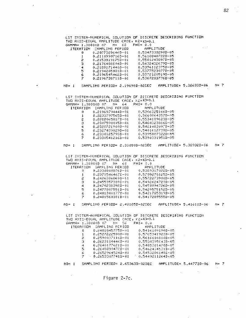
82

LST SYSTEM-NUMERICAL SOLUTION OF DISCRETE DESCRIBING FUNCTIONTWiO AXIS-EQUAL AMPLITUDE CASE, K2=K3=0.1GAMMA= 1.38000D 07 N= 68 PHI= 0.0

ITERATION SAMPLING PERIOD AMPLITUDE0 0.2 077:389646D- 11 0.5347338290D- 051 0 0.5618848722D-052 0.21538919175D-01 0.5501243897D-053 0.21764:3804D-01 0.5432432679D-054 0.21881714401-01 0.5396112:375D-055 0.21942050::-01 0 0.5377523077D-056 0.2196545462D-01 0.53721205191-057 0.2196738711D-01 0.5367283776D-05

ND= 1 SAMPLING PERIOD= 2.19698D-02SEC AMPLITUDE= 5.36633D-06 N= 7

LST SYSTEM-NIUMERICAL SOLUTION OF DISCRETE DESCRIBING FUNCTIONTWO A:IS-EQUAL AMPLITUDE CASE, ?:2=K3=0.1GAMMA= 1.3800D 07 [= 64 PHI= 0.0

ITERATION SAMPLING PERIOD AMPLITUDE0 0.2196979444D-01 0.53 2 '516 - 51 0. 2233797565D-01 0.5 660t64357D-052 0.22E:2065817D-01 0. 55i341:962:30-053 0.2307590015D-01 0.54 v60323816D-04 0.2320721900D- 1 0.542143097D- 055 0.23274:=:'9029D-01 0.54 161273:D- 056. 0.23:3 0325793- 01 0.5:-95 0:7322'D- 057 0.2330541216D-01 0. 5390:331951 D- 05

ND= I SAMPLING PERIOD= 2.33030D-O2SEC AMPLITUDE= 5.389321D-06 N= 7

LST S'YSTEM-NUPIERICAL SOLUTION OF DISCRETE DESCRIBING FUNCTIONTWO AXIS-EQUAL AMPLITUDE CASE, K2=E3=0.GAMMA= 1 .3800D 07 [4= 60 PHI= 0.0

ITERATION SAMPL I MG PERIOD HMPL I TUDE0 0 .23: 080087D-0 1 0.53893 17022-051 0.23715464671D-01 0.5709270125D-052 0.2426::3::6:69D-01 0.5572273900D-053 0 .2455:-357389 1- 01 0. 54926 24723D- 054 0.2470238:392- 01 0.545 08'9-4 726D- 055 0.2477837551D- 01 0.5429575152 - 056 0.2481:3 O00177D- 01 0.542 1785319D- 057 0.248156 0381D-01 0.5417289555D-05

ND= I SAMPLING PERIOD= 2.4185D-O2SEC AMPLITUDE= 5.416110-06 N= 7

LST :SYS:TEM-IIUMERICAFL :SOLUTION OF DISCRETE DESCPIBING FUNCTIONTWO A XIS-ECUAIRL AMFLITUDE CASE, K2=K3=0.1GAMMA= 1.38000D 07 = 56 PHI= i0.

ITERATION :zAMPLING PEPIID FMFLI TUDE0 0.2481 :45775.-1 1 41 r0.541 109190D-051 0.2527222590D-01 0.576341923D- 052 0.25900371161-01 0 .561661610D-053 0.2623180446D- 01 0. 55:30- l95 0l4:D- 054 0.26401 77621 D-01 II .54 :5-:3 1470D- 055 0. 2648::-'39 0472 B- 01 0.54624:345S3I1 D- 056 0.2652964524D- 01 0.54532:36 14D-057 0.2653307741D-01 0.5449211264 D-05

ND= 1 SAMPLING PERIOD= 2.65363D-02SEC AMPLITUDE= 5.44773D-06 N= 7

Figure 2-7c.

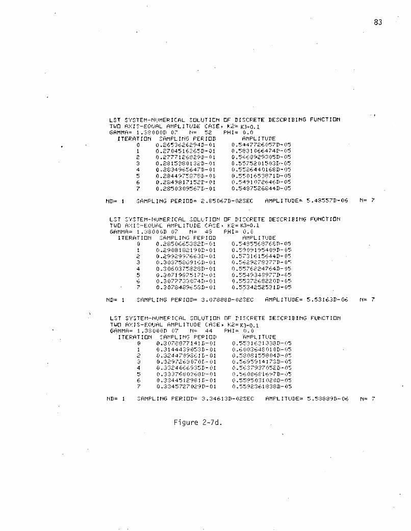
83

LST SYSTEM-NUMERICAL SOLUTION OF DISCRETE DESCRIBING FUNCTIONTWO A IS-EQUAL AMPLITUDE CASE, K2= K3=0.1GAMMA= 1.3:-000D 07 N= 52 PHI= 0i.0

ITERATION SAMPLING PERIOD AMPLITUDE0 0. 265:3626294D- 01 0.5447726057D-051 0.2704516:365D- 01 0.5831066474D-052 0.2777126:29D-01 0.5668929305D-053 0.28:15 38 132D-01 0.557 5201503ID- 054 0.2834965647D-01 0.5526440168D-055 0.2844975:37SD- 01 0.5501653871D-056 0.2849817152D-01 0.5491 072646D-057 0.2850309567D-01 0.5487526844D-05

ND= 1 SAMPLING PERIOD= 2.85067D-O02SEC AMPLITUDE= 5.48557D-06 N= 7

LST SYSTEM-NUMERICAL SOLUTION OF DISCRETE DESCRIBING FUNCTIONTWO AAI-EQUAL AMPLITUDE CASE, K'C=K3=0.1GAMMA= 1.::8000 07 N= 4: PHI= 0.0

ITERATION SAMPLING PEIOD AMPL I TUDE0 0 .2:8506653:82D- 01 0.548556:?768D- 051 0.299 08 1 :3: 21 '9 CD - 01 0.59091954 09D -052 0.299 2997663-01 0 .57:-.1615644D- 053 0.3037586916D-01 0.5629278377D- 054 0 .3 06 03752:E:D- 01 0.5576224764D- 055 0.30719:8 7517D-01 0.5549348977D-056 0.3 077733 074D-01 0.55:3726: -220D-057 0.307848965SD-01 0.5534252531D-05

ND= 1 SAMPLING PERIOD= 3.07888D-02SEC AMPLITUDE= 5.53163D-06 N= 7

LST SYSTEM-NUMERICAL SOLUTION OF DISCRETE DESCRIBING FUNCTIONTWO AX, IS-EQUAL AMPLITUDE CASE, K2=K3=0.1GAMMA= 1 .3:000D 07 N= 44 PHI= 0.0

ITERATION SAMPLING PERIOD HMPLITUDE0 0.3078877141D-01 0 .551-, 338D- 051 0.314443905:31 -01 1:1.600: 348 1 0D- 052 0.3244709:361D-01 0 .500-81558 04D- 053 0.329726307 :0D- 01 0.56 9591417:3D-054 0.3324066935D- 01 0.5 37937052D-055 0 . 33376 036:D- 01 0 .560 E:6 169 7- -056 0 .3:344512931 I 1D- 01 0. 55953102 O- 057 0.3-:45727 029- 01 0 .559 618 -05

ND= 1 SAMPLING PERIOD= 3.34613D-02SEC AMPLITUDE= 5.5:889D-06 N= 7

Figure 2-7d.

84

LST SYSTEM-NUMEPICAL SOLUTION OF DISCRETE DESCRIBING FUNCTIONTWO AXA:IS-EQUAL AMPIFLITUDE CASE K2=K3=0.1GAM'MA= 1.3800D 07 N= 20 PHI= 0.0

ITERATION SAMPLING PERIOD AMPL ITUDE0 0.60000000D- 01 0.1000 00000D-041 0. 6480879984D-01 ' 0.7617629854D-052 0.6678026019D-01 0 .71724931:389D- 053 0. 676928212 0 i- 01 0 .69968221 ':,D- 054 0.6813043341D-01 0.691848315 0D- 055 0.6834250429 D-01 0.63-88,25311 39D- 056 0.6843089594D-01 0.6:36190612D- 057 0.6844645543D- 01 0 .6858162908D-058 0.6846072173D-01 0.685474493011-05

ND= 1 SAMPLING PERIOD= 6.84679D-02SEC AMPLITUDE= 6.551690-06 N= 8

LST S'Y':STEM-NUMERICAL ::CLUTION OF DI::CETE DESCRIBING FUNCTIONTWO AXIS:-EOUAL AMPLITUDE CASE K2=,3=0.1GAFIMA= 1 .30001 07 N= 24 PHI= 0;0

ITERATIO1N SA IMPL I G PERIDD HMPL I TUDE0 0.6846787904D-01 '0 .6 51692663D- 151 0.673963903D- 01 0. 38497353D-052 0. E6:3:37165:D- 01 0. 46536444341D- 053 0.5831592193D-01 0.51185555170-054 0 .5 7251478:.33: - 1:11 0. E 1 i:6 5 :. 163::1D- 055 0.57:3697257'9D-01 0.6478E:453- 056 0. 579233375D- 01 0 . 64355::12, ::-057 0.5820893'924D-01 0.6406344573D-058 0 . 535654751ID-01 0 .6390 0:: 09'- 059 0.5842629652D-01 0.6 :35681 095D- 05

10 0.5342870822D-01 0.6:3:123: 65D-

ND= 1 SAMPLING PERIOD= 5.84322D-02SEC AMPLITUDE= 6.:3:1061-06 N=10

LST SYSTEM-NUMER I CAL :]OLUTION OF DIS'CRETE DESCRIBING FUNCTIONTWD AXIS-EQUAL AMPLITUDE CAiSE K2=K3=0.1GAMMA= 1.3:: 001 07 N= S PHI= 0.0

I TERRTI ON SMFLING PER IOD AMFL ITUDE0 0.584:3215529l-01 0.6 106:3121D-051 0.582029604D- 01 0 .4079:3611834D-052 0.55 ::04677 D- 01 0.4 70 3'8:3'739D- 053 0 . 531 824 2;8 04D1- 01 0. 529 :: 7351D-054 0.521 02 114 3D -01 0.56504672270-055 0.5152852903 D-01 0;5858 -912969D-056 0.51 24344: :i-'D - C 1 1.5 9726 0474: D- 057 0. 5111 415 171-01 .1 0529 - 058 0.51r0604657:- 0 1 ). 6 056801:3:::D- 059 0.5095:302379-01 0.61009:71101D-05

10 0.50r9564:3 64D- 0 1 0.60:387394 2 D-0511 0.5095120443D-01 0.6074 0:4692D- 0512 0 .5 09637825D- 0.608 0501700D-0513 0.509694005D-01 0.607795515;83D-05

ND= 1 SAMPLIHG PERIOD= 5.09695D-I025EC AMPL-ITUDE= 6.07877D-06 N=13

Figure 2-7e.

85

LST SYSTEM-NUMERICAL SOLUTION OF DISCRETE DESCRIBING FUNCTIONTWO AXIS-EQUAL AMPLITUDE CA':E K2=K3=0.1

GAMMA= 1.-::::000D 07 N= 32 PHI= 0.0ITERATION SAMPLING PERIOD AMPLITUDE

0 0).509694520D11-01 0.6078770868D-051 0.5102497922D-01 0.4119164140D-052; 0.4843472::24D-C01 0.4757019016D- 05

3 0 .46396:36 02D- 01 0. 52262346:- 9D- 05

4 0.460457:323D-01 0.5527945186D- 055 0.45602021 05D- 01 0.5702210947D- 056 0. 4538:::3-5611 :3D- 1 0.5795155652D- 057 0. 452792129'-D-i1 0.5941551842D- 1158 0.4 52144665D-01 0.5 8 662129585D-059 0.4547:300879D- 11 0. 5727916:3D- 05

10 0.4526 156 08D-01 II .514 044194D- 05

11 ) .4537422954D- 1 0.5-:54147556D -05

12 0. 4524681043 D- 01 0.51198'353 D- 051:3 0 . 4564413164D-01 l . 560 8',709:'70D- 0514 0.4E63:-:4 E 5 :-:6:3D- 01 0 .5:- 274 16 1D- 1:1515 0.4 573 02: 770 D- 01 0.5 87044 911 D- 05

16 0. 4545788:-3E:29D-01 0. 587:7-::2757D- 05

17 0.45:3 0423: 077 - 1 I' .5:E 699'.j79 5

1: 0.45193 :52759D- 0: 1 11 .59 :::' 07571-D 15

19 0. 451864604 6D- 01 0 . 5-:::5245069 D - 05

20 0.451875651:D- 01 0 .58:722E 00 '-'6D- 05

ND= 1 SAMPLING PERIOD= 4.511876D- 02:'5EC AMPLITIUDE= 5 .-37228D- 16 N=2 0

LST SYSTEM-NUMI1ERICL :C-LUTIONr OF DISCRETE DESCRIBING FUNC:TIONTWIAD A:ISC-EQUAL AMPLITUIDE CA:SE K2=K3=0.1GAMMA= 1 .3 07 I = -:36 PHI= 0.1

ITERATION :SAti PL INiG PERIOD AMPL I TUDE0 0.4518756513:D-01 0 .5:872280096D- 051 0. 454441 2051:- 01 I1. 4079529734D- -052 0. 4 19492135£1- 01 0 .470481 :3647D- 053 0.418 7535::37D-- 01 0.5152752542D-054 0.4116129664D-01 i. 54::3:385 20:30D- 055 0.4079400964D-01 0. 5593:4233 7 6D-I056 0.4 0615 1 :E:: D- 1 0.567: 0914:3D-05

7 0. 40545: 0647D - 01 0.5719556013D-058 0.4 0517154 01D- 01 0 .57384 -37457D- 059 0.405"2024514D-01 0.5733467174D-05

ND= 1 SAMPLING FERIDD= 4.05284D-02SEC AMPLITUDE= 5.72936D-06 N= 9

Figure 2-7f.

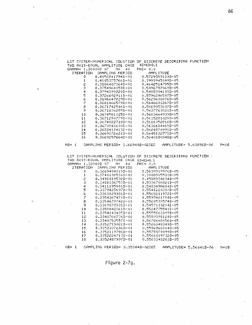
86

LST SYSTEM-NUMEPICAL SOLUTION OF DISCRETE DESCRIBING FUNCTIONTLO AXIS-EUAL AMPLITUDE CASE K2=K3=0.1GAMMA= 1.380001D 07 N= 40 PHI= 0.0

ITERATION SAMPLING PERIOD AMPLITUDE0 0.40523841794D-01 0.5 729:3 59'1:1D-051 0.4 105:375766 . 0 1 C.3 .'" 4 099D-C152 0.3:86407364D-01 0. 464l2514735D-053 0.3754'964:-:50ID- 01 0.5096797069D- 054 0.3794399220D-01 0.545: 041 O:D-055 0.3726602911 D-Ol 0.5596246507D-056 0.3696647229D- 0l1 0.5629'B:38876D-057 0.3681466579D-01 0.5646601 267Di- 058 0.3671 742546D- 01 0.566905:3607D-059 0.36718::36255D- 01 0. 563776:3:E 1 D- 0510 0.3674581125,- 01 0.561 6.64939D- i0511 0 .6712907791D-01 0. 56: 5 2 0 29D- 0512 03674 02271:D- 01 - .561 6052818D-0513 0.367094 069 1:- 01 0. 56366 :446911- 0514 0.3672410413 1D-01 0.562 4:-::74991D-0515 0 3669172621 D- 0 0.5645 1 :3277D-0516 0. :669257664D- 01 0.5641 -:0:348D- 05

ND= 1 SAMPLING PERIOD= 3.66940D-02EC AMPLITUDE= 5.638392D-06 N=16

LST SYSTEM-NUMERICRL SCLUTION OF DISCRETE DESCRIBING FUNCTIONTU. AX>IS-EiIIUAL AMPL I TUDE CASE E K2=K3=0.1GAMMA= 1.38OD 07 rN= 44 PHI= 0.0

ITERATO I ON HMPL INIG PERIOD AMPL ITUDE0 0. 36694040 1 9D- 01 0.56:3 :9' 19976D- 051 0. 74 01: 5:-: -01 0. ::9 0 1 553:D- 05S 0.349 1105'2D-01 0.45' , '46 34D-05

3 0.34 1 136753D-01 0. 5:--,670:21 D- 054 0.3411 195900ID- 01 0. 54:-:498604D- 055 0.379425697D-01 0.554122030iD-056 0. :::::3363829.;::3:1 D- 1 0.5568211972D- 057 0.335436740-01 0.55934 17 04D- 058 0. 35467.8.' 42-01 0. 55605574D- 059 0.3 87893 D-01 0. 5457110 14 D - 05

10 0. ::358042 :361riD- 0 1 0.5524775541D-0511 0 .3:54143435D- 0 1 0.5555863009'D- 0512 0. :34:E:'667316 D- 01 0.5589398 OD- 0513 0. 334','75: 3557D- C-01 0. 567.866:3056D- 0514 0.3- t352 71-081 D- 01 0 .556 434349D- 0515 0. :3:5 2:-:-37 6: D- 01 0. 5596966E.::64D- 0516 0. .352 1 1 '786D- 0 1 0.5575 7009; 'D- 0517 0.3 522-2471:-D- 01 I0.5566019732D-05

18 0 .335: 24879 7D-01 0 .556 43263D-05

ND= 1 SAMPLING PERIOD= :3.35304D-02SEC AMPLITUDE= 5.56041D-06 N=18

Figure 2-7g.

87

LN 81

LST SYSTEM-NUMEPICRL SOLUTION OF DISCRETE DESCRIBING FUNCTIONTWO A:-IS-EQUAL AMPLITUDE CASE K2=K3=0.1GAMMA= 1 .3:000 07 N= 20 PHI= 0.0

ITERATION SAMPLING PERIOD AMPLITUDE0 0.600000000000D-01 0.1000000000D-041 0.6480879'?9::4D-01 0 .76169854D- 052 0.6678026019D-01 A.7172493189D-053 0.6769282120D-01 0.69968:22188D-054 0.6813043:341D-01 0.6'1. 4 3150D-055 0.6834250429D-01 0.6882531139D-056 0.684 30:39594D- 01 0 .6:68190612D-057 0.6844645543D-01 0.6E:58162908D-058 0.6846072173D-01 0.6854744930D-05

ND= I SAMPLING PERIOD= 6.84679D-02SEC AMPLITUDE = 6.85169D-06 N= 8

LST SYSTEM-NUMIIERICAL SOLUTION OF DISCRETE DESCRIBING FUNCTIONTWO AXIS-EQUAL AMPLITUDE CASE K2=K3=0.1

GAMMA= 1..38:O00OD 07 N= 18 PHI= 0.0ITERATION SAMPLINIG PERIOD AMPLITUDE

0 0.6846787904D-01 0 .685169266D- 051 0.704325670D-01 0. 74942:37996D- 052 0.7274274026D-01 0.7:35:35732 78 D- 053 0.7391256151D-01 0.727 00: 0744 8 D- 054 0.7449677609D-01 0.722462 22D- 055 0. 747896721 6D1- 01 0 .7201 21959:_:D- 056 0.7494085861 D-01 0 .71 :9269556D- 057 0.7500155196 D-01 0.718793:6355D- 05

ND= 1 SAMPLING PERIOD= 7.50031D-O2SEC AMPLITUDE= 7.13146D-06 N= 7

LST SYSTEM-NUMERICAL SOLUTION OF I:SCPETE DE:::CRIFINMG FUNCTIONTWO A:.::I-EUIAL AMFLITUDE CASE K2=K3=0.1GAMMA= 1.3',0OO Di 07 = 1 PHI= 0.0

ITERATION SAMPLING PERIOD AMPL I TUDE0 0. 750013876D-01 0.71E1455222D-051 0.7757207225D- 01 0.7904102565D-052 0.80:3652652':r D- 01 A0.773:556,:32- 053 0.81771016::4 4D- 01 0.769932 9912D- 054 0.82471 5781511D-0 1 0. 7654031 462D- 055 0.8::282203857D - 01 0.7E1003421 D-056 0.330018::79:D- 01 0. 76 1,9;0625:6::6I- 057 0.83091 00145D- 01 .76156774 1D- 058 0.8:3:092497 07D- 01 0.7610629302D- 05

ND= I SAMPLING PERIOD= :E..30950D- 02EEC AMPLITUDE= 7.61094D-06 N= :3

LST SYSTEM-NUMEPICAL SOLUTION OF DI CRETE DESCR IPING FUNCTIONTWO AX:I-EIAIRL AMPLITIIDE CASE K2=K3=0.1GAMMA= 1. -:3 000 0 17 N= 14 PHI= 0.0

ITERATION :AMIF'L I Ni PER IO D RMPLITUIDE0 0.8309501 07:3D-01 0. 1 09? 76 09 D - 051 0.8671 .:9 02D-01 . 14_0 642551D- i052 0.9017647994D-01 0 1 -:91106D-053 0.919 069 13::-:- i0.1 0 . 46 749-: D- 05

4 .9 76:1 1: D-01 0 . : 5510559 - 055 0.9319:361204 D- 01 0. :1: 455:99_D- 056 0 .934175 0696D- 01 0. 17:358:3:624 D- 057 0.9:353493942D-01 0. 1 6872384 9D- 058 0.9.35394 1607D- 01 0.8167792323D- 05

ND= 1 SAMPLING PERIOD= 9.35426D-02SEC AMPLITUDE= 8.16689D-06 N= 8

Figure 2-7h.

88

LST SYSTEM-NUMERICAL TOLUTION OF DISCRETE DESCRIBING FUNCTIONTWO AXIS-EQUAL AMPLITUDE CASE K2=K3=0.1GAMMR= 1 .3000 7 N=. 12 PHI= 0.13

ITERATION SAMPLING PERIOD AMPLITUDE0 0.93:54264774D- '01 0. 816683:857: 99- 051 0.991611 :2:2221D-01 0.: 9'90156255D-052 0.1 035439723D 00 0 .898t4162026D-053 0.1057325363-:iD 0 0.8'9441192761D-054 0.1068237479D 00 0.8916745965D-055 0.1 07366 1191D 00 0 .3'?9022070341D-056 0.1076409935D 00 0.3:39451:3616D-057 0.107788 799371 00 0.8390091772 D- 058 0.1078160524D 001 0.8894539016D-05

ND= 1 SAMPLING PERIOD= 1.07818D-01SEC AMPLITUDE= 8.88944D-06 N= 8

LST SYSTEM-NUMERICAL ::OLUTION OF DISCRETE DESCRIBING FUNCTIONTWO AXIS-EQUAL AMPLITUDE CASE K2=K3=0.1GAMMA= 1.38:000D 07 NI= 10) PHI= 0.0

ITERATION O SAMPLING PERIOD AMPL ITUIDE0 0.10781 7113D 0 0.8359444'-r:D-051 0.11771005'971D 0 0.962 1415477 D-52 0.1232336219 00 0.98013655 17D-053 0.126 050:324:3-: 00 0.9.-40692922D- 054 0.12746396:8CD 00 0.9:3492119 26D-055 0.1 2 8 1670330) 00 0.9::52245:354D- 056 0.12 851 901D 00 0.9 -: 85 311699 D- 057 0.1287 044745D 00 0.:5:::669021-058 0.1 28819 633:3D1 00 0.9:552-5553D-05

ND= 1 SAMPLING PERIOD= 1.2::8820D-01 SEC AMPLITUDE= 9.85437D-06 N= 8

LST SY'STEM-NIUMERICAL SOLUTION OF DISCRETE DESCRIBING FUNCTIDNTI.lO AXIS-EQUAL AMPLITUDE -CAS:E K2=K3=0.1GAMMA= 1.3:83o00rD 07 N= 8 PHI= 0.0

ITERATION SAMPL IG PERIOD AMPL I TUDE0 0.123:881958751D 00 0.9854:3657740-051 0.1497371:337 1 00 0. 101982:'2965 0D- 042 0.15582 085:32D 00 0. 108:0467416D-043 0. 159:37.3:457D 00 0. 1102825J25D-044 0.16120071:8E:D 00 0.111263557:-:D-045 0.16211:35626D 00 0.1117426051D-046 0. 16 25677190D 00 0. 1119:856757D- 047 0.1628001760D 00 0.1121022683D-048 0.1629475305D 00 0.1121329115D-04

ND= 1 SAMPLING PERIOD= 1.62948D-OISEC AMPLITUDE= 1.12223D-05 N= 8

LST SY'STEM-NUIMERICAL SOLUTION OF DI :-CRETE DESCRIBING FULINCTIONTWO AX:IS-EQUAL AMPLITU'DE CASE K2=K3=0.1

GAMMA= 1.3:8000D 01 N= 6 PHI= 0.0ITERTION SHMPLING PERIOD AMPLITUDE

0 0.162.-948E:3722D 00 0.1122229409D-041 0.2218967506D 00 0. 1065971960D-042 0.22: 36 417:39D 0 0 .1979 0559D-043 0.227510:3S1D 00 0.1256521127D-044 0.2 295949249D 00 0 12E62 1146D-045 0.2306573515 00 0 .1301572755D-046 0.2311:9602D 00 0 .3037 43:39D- 047 0.2314570519D 0 0 1 31 3136:39D-048 0.2:315967783D 00 0.1315256779D-049 0.2317193751D 00 0. 1315921728D-04

ND= 1 SAMPLING PERIOD= 2.316951)-OSEC AMPLITUDE= 1.31578D-05 N= 9

Figure 2-7i.

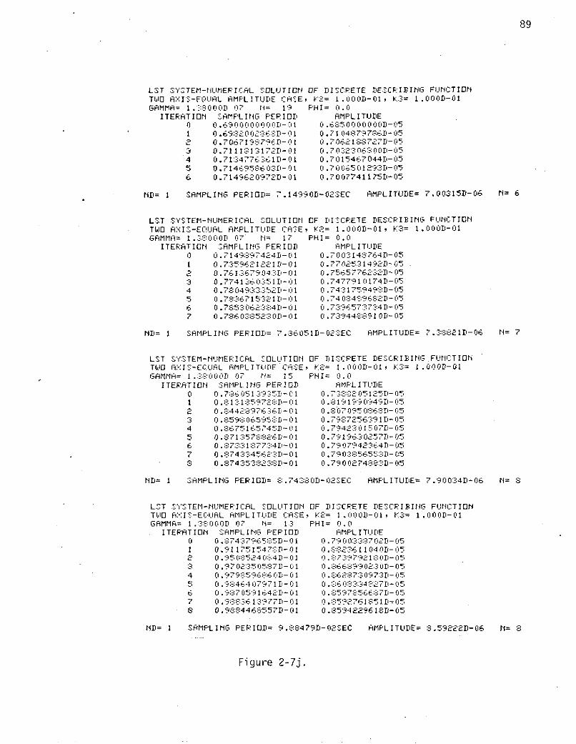
89

LST SYSTEM-NUMEFICAL SOLUTION OF DISCRETE DESCRIBING FUNCTIDNTWO AXIS-EQUAL AMPLITUDE CASE, K2= 1.000D-01, K3: 1.000D-01GAMMA= 1.:38000 07 rl= 19 PHI= 0.0

ITERATION SAMPLING PERIOD AMPLITUDE0 0.69000000001-01 0 .6850 000000D-05I 0.698:200E:6:D- 01 0.710487976D-052 0. 067198796D-01 .706E2188727D-053 0.7111813172D-01 0.70323063001-054 0.7134776361D-01 0.7015467044D-055 0.7 14695: 603D-01 0.70106501293D-056 0.7149620972D-01 0.7007741175D-05

ND= 1 SAMPLING PERIOD= 7.14990D-02SEC AMPLITUDE= 7.00315D-06 N= 6

LST SYSTEM-NUMERICAL SOLUTION OF DISCRETE DESCRIBING FUNCTIONTWO AXIS-EQUAL AMPLITUDE CACSE K2= 1.000D-01, K3= 1.0000-01GAMMA= 1.:-:80001D 07 N= 17 PHI= 0.0

ITERAT ION SA:MPLING PERIOD AMPLITUDE0 0.7149897424D-01 0.7003148764D-051 0.7359621221D-01 0 .7702531492D-05

2 0.7613679043D-01 0.7565776232D- 05

3 0. 7741:36035 1D- 01 0.7477910174D1-054 0 .7:3 049 3:3:-:3352D-0 1 0.74:3175949S:D- 1055 0.78:367153::211D-0:11 0 .74 0:34::962D- 056 0.7853062::38E:4D-01 0.7:396?573734 D- 057 0.7860385230D-01 0.7394488910D-05

ND= 1 SAMPLING PERID= 7.86051D-02SEC AMPLITUDE= 7.38821D-06 N= 7

LST SYSTEM-NUMERICAL SOLUTION OF DISCRETE DESCRIBING FUNCTIONTWO AXIS-EQUAL AMPLITUDE CASE, K2 = 1.000D-01 K1-3= 1 .000D-01GAMMA= 1.3:30003 07 N= 15 PHI= 0.0

ITERAT ION SHAMPLING PERIOD AMFL I TUDE0 0 .786 051 393:5D- 1 0. 7:38: 2 05 125D- 051 0 8:31:31.59 72:D- 01 0. 1919 0'949D-052 0 .442897636D- 01 0. :8:070950:6:1D-053 0.859E:86595:D- 01 0 .7987256391D-054 0.867 5 16 5 745 D-01 0.7942301507D-055 0.87135788-26D-0 0.7919630257D-056 0. 73318:7734D-01 0. 7907942364D-057 0.874:3:34562:3D-01 0.7903856553D-058 0.87435::8:3823D-01 0.7900274883D-05

ND= 1 SAMPLING PERIOD= :.74380D-02SEC AMPLITUDE= 7.90034D-06 N= 3

LST SYSTEM-NUMERICAL SDLUTIION OF DISCRETE DESCRIBING FUNCTIONTWO AXIIS:-ECUAL AMPLITUDE CASE, K2= 1.000D-1O K3= 1.000D-01GAMMA= 1.,3:8000D 07 N= 13 PHI= 0.0

ITERATION :SAMPLIrG PEPIOD AMPL ITUDE0 0 .:744379655D- 01 0.7900:z:3:37 02D- 051 0.911751547D- 01 0.88:361104 0D- 052 0.950824084D- 01 0.87397918 I- 053 0.9702:350587D- 01 0. 6689902'30D- 054 0.979859686 OD-01 0 .:.62873:3097:31- 055 0.98464 0771D- 01 0 .60:34:7D-056 0.9:370591642D- 01 0 .8597856687D - 0 5

7 0.9383613977D- 01 0 .:3592761851D- 058 0.9884468557D-01 0.8594229618D-05

ND= I SAMPLING PERIOD= 9.S8479D-O2SEC AMPLITUDE= 8.59222D-06 N= 8

Figure 2-7j.

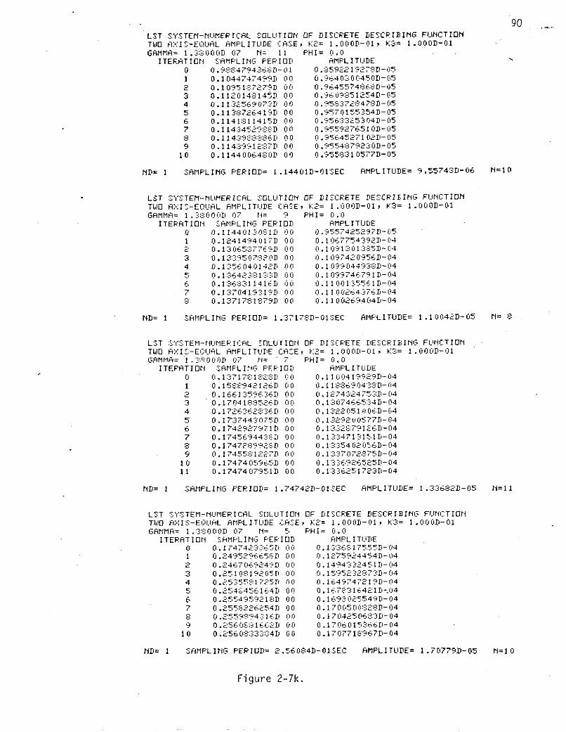
90LST SYSTEM-NUMERICAL SOLUTION OF DISCRETE DESCRIBING FUNCTIONTWO AXIS-EQUAL AMPLITUDE CASE, K2= I.O00D-01, K3= 1.000D-01GAMMA= 1.3:8:000D 07 N= 11 PHI= 0.0

ITERATION SAMPLING PERIOD AMPLITUDE0 0. 84794368D- 01 0.8592219278D-051 0.1044747499D O0 0.9640:3 00450D-05

2 0.10951::7279D 00 0.9645574868D-053 0.112014848145D 00 0.9609:51254D-054 0.1132569073D 00 0.958:3728478D-055 0.1138726419D 00 0.9570155354D-056 0.1141811415D 00 0.9563-253 04D- 057 0.114:34529:E:SD 00 0.9559276510D- 058 0.114:39 :-86D 00 0.956452-71f02D-059 0.11439912:87D 00 0.95548 792:30D- 05

10 0.1144006480D 00 0.9558310577D-05

ND= I SAMPLING PERIOD= 1.14401D-01S.EC AMPLITUDE= 9.55743D-06 N=10

LST SYSTEM-NUMERICAL SOLUTION OF DISCRETE DESCRIBING FUNCTIONTWO AXIS-EOLIAL AMPLITUDE CASE, K2= 1.00OOD-01, K3= 1.000D-01GAMMA= 1.3:3000D 07 N= 9 PHI= 0.0

ITERATION SAMPLING PERIOD AMPLITUDE0 0.114401.3081D 00 0.9557425297D-051 0.1241494 017D 00 0. 1 067754392D- 042 0. 13065I7769D 00 0 . 1091 :: 301 ::5D- 043 0.13395078:20D 00 0.1 097420956D-044 0. 1356 04 01 42D 0 00. 109 9 044938D-04

5 0.1:364238 1:3 :: D 00 0. 1 099746.79'ID- 046 0. 1:36:311416 D 00 0. 11 00135561D-047 0.1370419319D 00 0.1 100264:376D- 048 0.13717813879D 00 0. 100269404D-04

ND= 1 :SAMPLING PERIOD= 1.3717',D-O1SEC AMPLITUDE= 1.10042D-05 N= :8

LST :S:STEM-IUMERICAL SOLUTION OF DISCRETE DESCRIBINI FUNCTIONTWO AXIS-EOUAL FAMPLITUDE CASE, K2= 1.000D-01j, K3= 1.000D-01GAMMA= 1. 3000: D 07 N= * 7 PHI= 0.0

ITERAT ION SAMFPL ING PERIOD AMPL ITUDE0 0.1:3717 1:E:D :00 0.110041 9929D- 041 0.158:942126D 00 0.1 1:8869043D- 042 0.1661:359636D 00 0.1274:324753D-043 0. 1704 :188526D 00 0. 1307466534 D- 044 0.1726362:36D 00 0.1322051 0061D-045 0. 1 37443075D 00 0.1329200577D-046 0.1742927971 I 00 0.13:32,:79126D-047 0.17456944:38::D 00 0. 1 3:347 :3151D-048 0. 17472'8992:D 00 0.13I 35402 O056D- 049 0.174551227D 00 0.1337072875D-04

10 0.1747405965D 00 0.1:3:-:6525D-0411 0.1747407951D 00 0.1:336251723D- 04

ND= 1 SAMPLING PERIOD= 1.74742D-01SEC AMPLITUDE= 1.33682D-05 N=11

LST SYSTEM-NUMERICAL SOLUTION OF DISCRETE DESCRIBING FUNCTIONTWO AXIS-EQUAL AMPLITUDE CASE, KE'= 1.000D-O1, K3= 1.00OD-01GAMMA= .:3000:D 07 N= 5 PHI= 0.0

ITERATION SAMPLIN1G PERIOD HMPLITUDE0 0.1747423":65D 00 0. 1 :36:- 17555D- 041 0.249529665:DD 00 0. 1275944454D-042 0.24670692e49D 00 0.1494332451D -043 0.2510:3 19205D 00 0.1595 23287 D- 044 0.25551725D 00 0.1649747219D-045 0.254:456164D 00 0.1 67:316421D11-46 0.2554959218D 00 0. 1693025549D-047 0.255:3226254D 00 0.1700500:28D-048 0.2 59294316D 00 0.170425063D- 049 0.2560881E662D 00 0.1706015366D-04

10 0 .25608:333:34D 00 0.1707718967D-04

ND= I SAMPLING PERIOD= 2.56084D-OlSEC AMPLITUDE= 1.70779D-05 N=10

Figure 2-7k.

91

LST SYSTEM-NUMERICAL :SOLUTION OF DISCRETE DESCRIBING FUNCTIONTWO AXIS-EQUAL AMPLITUDE CASE, K2= 1.000D-01, K3= 1.000D-01GAMMA= 1.38000D 07 N= 4 PHI= 9.00000 01

ITERATION SAMPLING PERIOD AMPLITUDE0 0.5000000OOD 00 0.1500000000D-041 0.5154240480D 0'0 0.1377904361D-042 0.5395948070D 00 0.1446567295D- 043 0.5480038734D 00 0. 147478 150D-044 0.55012:32936D 00 0.1486946298D- (-045 0.5498353305D O:0 0.149:33778981D-046 0.5496153256D 00 0.149676:3755D-047 0.54955191111D 00 0.1498535914D-048 0.5495572657D 00 0.1498126090D-04

ND= 1 SAMPLING PERIOD= 5.49637D-OISEC AMPLITUDE= 1.49913D-05 N= 8

LST SYSTEM-NUMERICAL SOLUTION OF DISCRETE DESCRIBING FUNCTIONTWO AXIS-EQUAL AMPLITUDE CASE, K2= 1.000D- 01 K3= 1.00D-01GAMM= 1.:38000D 1107 N= 4 PHI= s.0O0000D 01

ITERATION SAMPLING PERIOD AMPLITUDE0 0.5496365534D 00 0.1499127478D-04

2 5.49637-01 - .91174D-052 5.501861"-01 -1.956,88 -05

1 0.4234186796D 00 0.845454562303D-042 4.234191D-01 7.3180D-052 4.2:3842D-01 -7.458' 11D-05

2 0.3730698891D 00 0.1692422145D-043 0.4128434144D 00 .1637625694D-044 0.4312546179D 00 0. 1654907656D-045 0.4397401524D 00 0.1665122919D-046 0.4433010.96D 00 0 1670404294D-04

7 0.4458433195D 00 0. 1673064847D-048 0.4468524793D 00 0.16743908":33D--049 0.4473906822D 00 0.1675010719D-04

10 0.4475205608D 00 0.1675157026D-04

ND= 1 SAMPLING PERIOD= 4.47512D-O1SEC AMPLITUDE = 1.67488D-05 N=10

LST SYSTEM-NUMERICAL SOLUTION OF DISCRETE DESCFIEING FUNCTIONTWO AXIS-EQUAL AMPLITUDE CASE, K2= 1.000D-01, K3= 1.000D-01GAMMA= 1.380001 07 N= 4 PHI= 7.000001 01

ITERATION SAMPLIN G PERIOD AMPL I TUDE0 0.4475120178:1 00 0.1674881540D-041 0.42160:32457D 00 0. 1861170429D-042 0.4051047902 00 0. 1900082144D- 043 0.3938394079D 00 0.1918318637D-044 0.38676041543 00 0.1928180740D-045 0.38254 07502D 00 0.19:335254591D-046 0.3801177764D 00 0.1936336477D-047 0.3787622054D 00 0 .1937772905D-048 0.3780160288SD 00 0 .193492295 D-049 0.3776076550D 00 0.1938848190D- 04

10 0.3773823844D 00 0.1939023413D-04

ND= I SAMPLING PERIOD= 3.77255D-01SEC AMPLITUDE= 1.93911D-05 N=1 0

Figure 2-8a.

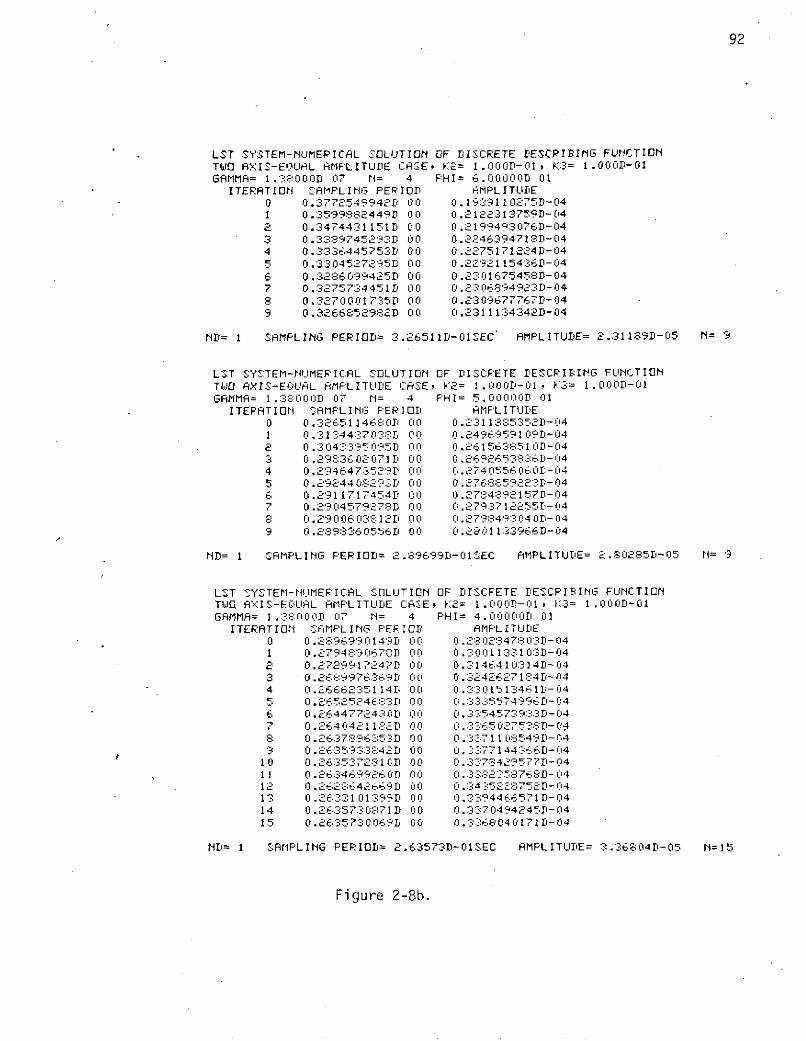
92

LST SYSTEM-NUMERICAL SOLUTION OF DISCRETE DESCRIBING FUNCTIONTWO AXIS-EQUAL AMPLITUDE CASE, K2= 1.000D-01, K:3= 1.000D-01GAMMA= 1.3: OOOD 07 N= 4 PHI= 6.00000D 01

ITERATION SAMPLING PERIOD )AMPL I TUDE0 0.3772549942D 00 0.19:39110275D-041 0.3599832449D 00 0.2122313759D-042 0.34744:31151D 00 0.2199493076D-043 0.3389745293D 00 0.2246394718D-044 0.3336445753D 00 0.2275171224D-045 0.3304527295D 00 0.2292115436D-046 0.3286099425D 00 0.2301675458D-047 0.3275734451D 00 0.23 06894923D-048 0.3270001735D 00 0.2309677767D-049 0.3266852982D 00 0.2311134342D-04

ND= 1 SAMPLING PERIOD= 3.26511D-OISEC AMPLITUDE= 2.31189D-05 N= 9

LST SYSTEM-NUMERICAL SDLUTION OF DISCFETE DESCRIlING FUNCTIONTWO AXIS-EQURL AMPLITUDE CASE, K2= 1.000D-01, K3= 1.00D-01GAMMA= 1.3;8000l 07 N= 4 PHI= 5.00000D 01

ITERATION "SAMPLING PERIOD AMPLITUDE0 0.32651146E0D 00 0.23113853,D-041 0.31344:3703-D 00 0.24969591 09D-042 0.:3043395 095D 00 0.261563:-510D- 043 0.2983602071 D 00 0.269265: C36D- 044 0.2946473529D 00 0.2 74 055, 16 0D!-0 45 0.29244 029:-D 00 0. 2768659223D-046 0.2911717454D 00 0.278::492157D-047 0.2904579278D 00 0.279:3712255D- 048 0.29006 031 2D 00 0.279S 49340 oD- 049 0.2898360556D 00 0.2801133966D-04

ND= 1 SAMPLING PERIOD= 2.89699D-OISEC AMPLITUDE= 2.80285D-05 N= 9

LST SYSTEM-NUMERICAL SOLUTION OF DISCRETE DESCPIBIMG FUNCTIONTWO AXIS-EQUAL AMPLITUDE C:ASE, K2= 1.000D-01, :::3= 1.00OD-01GAMMA= .::O000D 07 N= 4 PHI= 4.00000D 01

ITERAT ION SIAMPL INc PERIOD AMPL ITUDE0 0.2896990149D 00 0.2:8028478 :03D-041 0.279489 0671D 00 0. :30011:3310:3--D- 042 0.2729917247D 00 0.3146410314D-043 0.2689976369D 00 0.:3242627184D-044 0.2666235114D 00 0 .:3:301513461D-045 0.2652524683D 00'l 0.335574996D- 046 0.2644772430D 00 0.354573933D-047 0.2640421182D 00 0.36502753-D-048 0.2637896353D o0 0 .: 71108549D- 049 0.263593 -- '4 21' 10 0 .. 77144366rD- 04 4

10 0.2635372810D 00 0.3-78429577D-0411 0.2634699260 D 00 0.:3:32358768D-0412 0 .2628642669D O0 0.345228752D-0413 0.26:33101:3991D 0 0.3394466571D-0414 0.2635730871D 00 0.337049424511- 0415 0.2635730069D 00 0.3:68040171D-04

ND= 1 SAMPLING PERIOD= 2.63573D-01SEC AMPLITU'E= 3.36804D-05 N=15

Figure 2-8b.

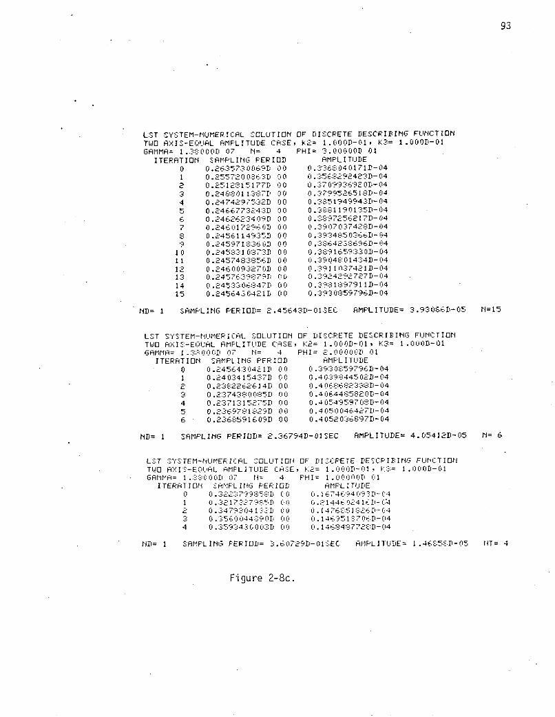
93

LST SYSTEM-NUMERICAL SOLUTION OF DISCRETE DESCRIBING FUNCTIONTWO AXIS-EIUJL AMPLITUDE CASE, K2= 1.00D-01, K3= 1.000D-01GAMMA= 1.8000D 07 N= 4 PHI= O3.000001 O1

ITERATION SAMPLING PERIOD AMPLITUDE0 0.2635730069D 00 0.33604171D-041 0.2557200863D 00 0.3568292423D-042 0.2512815177D 00 0.37099:36920D- 043 0.248:01 137D 00 0.3799526518D-044 0.2474297532D 00 0.3851949943D-045 .2466773243D 00 0.388:31190135D-046 0.2462623409D 00 0.3u9725621-D-047 0.2460 17296 0D O0 0.:' 907 037428D- 048 0.2456114935D 00 0.3:93485: 0366D- 049 0.245971:360D 00 0.38642'38696D-04

10 0.2458031073D 00 0.3 ::659330D-0411 0 .474385D 0 0 .34: 0144D - 0412 0.246009:A-270 00 0. 39110:37 42 1D- 0413 0.2457639879D 00 0.3924292727D-0414 0.2453306:-S47D 00 0 .39:31:979111D-1:0415 0.2456430421D 00 0.39"30:359796D- 04

ND= 1 SAMPLING PERIOD= 2.45643D-01SEC AMPLITIJDE= 3.93086D-05 N=15

LST SYSTEM-NUMERICAL SOLUTION OF DISCRETE DESCRIBING FUNCTIONTWO AXI :-EUI UAL AMPLITUDE CASE K2= 1. 001D-01 , K3= 1.000D-01GAMMA= 1.3;:I000D 07 N= 4 PHI= 2.00000DI 01

ITERATION SAMPLING PERIOD AMPLITUDE0 0.245643:-041D 00 0 .3 0:59796D-041 0.2403415437D 00 0.4039-44502D-042 0.235:2262614D 00 0.4 068682 3:38D- I04:3 0.2:374:3800::85D 00 0.4064485832 OD- 044 0.2 71:315275D 00 0.4054959 70D-045 0.2369781829D 00 0.4050046427D-046 0.2368591609D 00 0.4052036897D-04

ND= 1 SAMPLING PERIOD= 2.36794D-OISEC AMPLITUDE= 4.05412D-05 N= 6

LST SYSTEM-NUMERICAL SOLUTION OF DISCPETE DESCRIING FUNCTIONTWO A'I:S-EJ-UAi L RMPLITUDE CA:S:E, K2= 1.00Oi D- 01 K= 1.00011-01GAMMA= 1.::38 0D 1:17 N= 4 PHI= 1.O00i 00D 01

I TERR T I ON AMPL I NG PERI DD AMPL I TUDE0 0.3223799858D0 .167469409 :D-041 0. .: 2173 .5D 0 L.2144602416D-0"42 0. 3479304 13-:D 00 0.14076.516 - 043 0. 3560440D 0 .14 69 1 . 6D- I- 14

4 0.35934:3 000D 00 0.1464:877 28:D-04

ND= 1 SAMPLING PERIOD= 3.60729D-01 SEC ANRPLITUDE= 1.4685::D-05 HT= 4

Figure 2-8c.

94

0.12- -- I. . .. ..

K = 1.0 K = 0.1

00 Large n n=120.10

n=13

--.......................... 14S. n=15

n=18 .

n=200.06

.... n=24

n=32

0.04

n=40 .

n=600.02.1

n=80 . . . .

n=100

0.00 - ..-

5 6 7 8 9 10

Amplitude ( x 10-6

Figure 2-9. Amplitude and frequency (2n/nT) of self-sustained oscillations

for various sampling periods in the discrete-data two-axis LST

system; v = 1.38x107

95

1.2

K = 1.0 K =0.12 3n less than 13

1.0 600

S5400.8 n=3

480

0.6A 120 360F- . . .0. .

900 300

n=6 150

0.4 l-I \ 70 0600

100.- - 400 --- --- -300

n =6 o120:, - - 2000.2 16

n=12 ..

0.0 -- - -'_

0 1 2 3 4 5

Amplitude ( x10 - 5 )

Figure 2-10. Amplitude and frequency (2/nT) of self-sustained oscillations

for various sampling periods in the discrete-data two-axis LST

system; y = 1.38×107

96

0.08I n=28 .... . ..

_ _ ... ... K2 = 5 K = 0.10.07

. = 0 Large n.... .... ..........

n= 32 - -

0.06

i i ... : i

. ._: ! i i. ..

0.05

n'40

n=44

.... .... ... n=48

. I.... .. .......... On=52

I-I

n=680.03

.. ... .... .n=6 68

0.02. . . . . . . . . . . .

I :0.01

0.00 _0 5 10 15 20 25

Amplitude ( x10-7)

Figure 2-11. Amplitude and frequency (2r/nT) of self-sustained oscillations

for various sampling periods in the discrete-data two-axis LST

system; v = 1.38x107

97

REFERENCES

1. B. C. Kuo and G. Singh, Design of the Large Space Telescope System,Final Report, for NAS8-29853, Systems Research Laboratory, Champaign,Illinois, July 1, 1974.

2. B. C. Kuo and G. Singh, Continuous and Discrete Describing FunctionAnalysis of the LST System, Final Report, for NAS8-29853, SystemsResearch Laboratory, Champaign, Illinois, January 1, 1974.

98

3. Study of Unequal-Amplitude Oscillations in Two-Axis Coupled

Nonlinear Systems

3-1. Introduction

In the preceding two chapters conditions of self-sustained

oscillations in the two-axis LST system have been studied by a

numerical-iterative technique using the describing function. It

is demonstrated that the numerical-iterative technique can be applied

to the continuous-data as well as the discrete-data LST system. The

difference between these two types of systems lies only in the

stability equations, and these made no difference to the iterative

algorithm.

It is important to note that since the dynamics of the two

axes are identical, it is assumed a priori that the amplitudes of

oscillations, if there are any, are of equal amplitude. Certainly,

all the solutions of the self-sustained oscillations obtained in the

previous chapters are sinusoidal signals with equal amplitude in

both axes. However, in this chapter we shall show that, in general,

it is possible to have unequal magnitudes of oscillations in the

coupled system even if the dynamics of the two axes are identical.

Furthermore, when the amplitudes of oscillations are equal, the

phase can still be 180 degrees apart.

Since we have reasoned that the numerical-iterative technique

does not distinguish a continuous-data system from a discrete-data

system, only models of the former version are discussed here.

99

3-2. Conditions of Unequal-Amplitude Oscillations in The Continuous-

Data Two-Axis Coupled LST System

Figure 3-1 shows the signal flow graph of the continuous-data

two-axis model of the LST system. The inputs to the two nonlinearities

are designated as E1 (jw) and E2 (jw), respectively. Notice that these

two variables are complex quantities in general, and each represents

a magnitude and phase in the sinusoidal steady state. Since the

describing function of the CMG nonlinearity is a function of the

input amplitude and frequency, Fig. 3-1 shows that the describing

functions which correspond to E (jw) and E2 (jw) are N(El,w) and

N(E2 ,w), respectively. For simplicity, the following notations are

used:

El (j) = El

E2 (jw ) = E2

N(EI,w) = N1

N(E2'w) = N2

The transfer functions in Fig. 3-1 are defined as

(K + K1 s)KIG1 K+K(3-1)

1 KpS+ KI

Ks + K

G2 s (3-2)

G3 s (3-3)

100

-I

IGI _G2 G3 H G4X, =o 2 X3 1/ X4 5 /v

-N,El,

-K2

-K-

I G G G3 H G4

X2=O 2 Y3 /s Y4 Y5 H-N2

-I

Figure 3-1. The simplified continuous-data two-axisLST system model.

101

G4 2 v (3-4)s + K3s + K2

The determinant (characteristic equation) of the coupled system of

Fig. 3-1 is written

A = 1 + GA + GBlNl + GB2N2 + GCN N2 = 0 (3-5)

The last expression is also known as the stability equation of the

system.

The linear transfer functions in Eq. (3-5) are

GA = 2G2 G3 + 2G1 G2 G3 G4 H - K2G 4 + G2 G + (G1G2 G3 G4 H)2

+ 2G1G G G4H - 22GG 3 GK2 - G2G GK 2 (3-6)

G G 2 + 3 + (3-7)Bl B2 s s s s s

G2 G2G2 2

GC 2 2 (3-8)s s

Equation (3-5) represents a necessary condition for self-

sustained oscillations in the system of Fig. 3-1. However, in general,

if the amplitudes of E1 and E2 are not equal, Eq. (3-5) represents a

set of two nonlinear equations with four unknowns in E1 , E2, the

frequency w, and c, the phase between E1 and E2. Therefore, in

addition to the two equations which are obtained from the real and

imaginary parts of Eq. (3-5), a third complex equation must come from

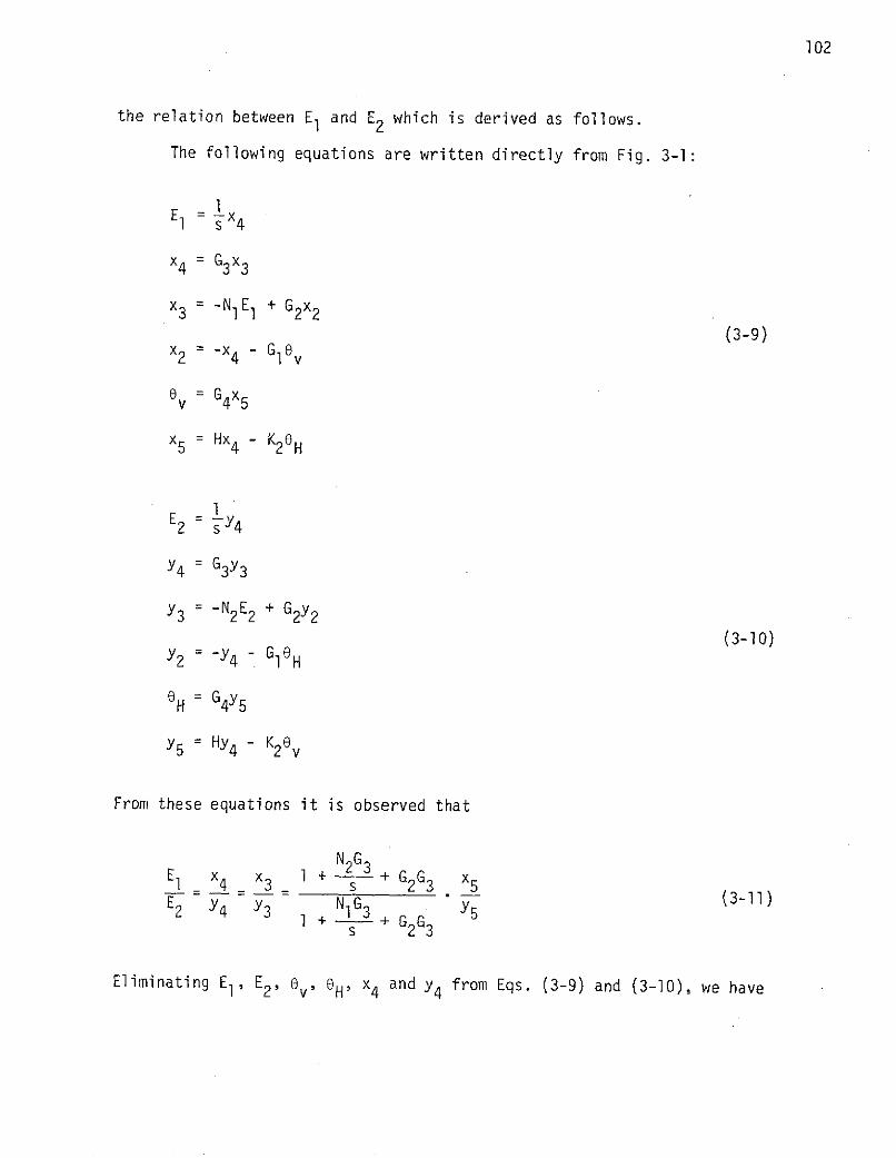
102

the relation between E and E2 which is derived as follows.

The following equations are written directly from Fig. 3-1:

1

x4 = G3 x3

x3 = -N 1 E + G2 x2

(3-9)x2 = -x4 - G1 ev

0v = G4x 5

x 5 = Hx4 - K2 H

12 = sY4

Y4 = G3Y3

Y3 = -N2 E2 + G2 Y2

(3-10)Y2 = -Y4 - GIeH

OH = G4 Y5

Y5 = Hy4 - K2 6v

From these equations it is observed that

N2G3E x x 1 + + GG3 x1 4 3 s 23 5

• - (3-11)E2 Y4 Y3 N1 G3

1 + s G2G3

Eliminating E1 , E2, 6, H, x4 and y4 from Eqs. (3-9) and (3-10), we have

103

N1G3x - x +Gx3 s 3 G2x2

x2 = -G3 x3 - G1 G4X 5 (3-12)

x5 = HG3x3 - K2G4 5

N2G3Y3 = - 3 + G 2Y2

2 = -G3Y3 - GI G4Y5 (3-13)

Y5 = HG3Y3 - K2 G4 x5

These equations are solved to yield

x5 1 +A 2 +B+C5 (3-14)

Y5 -K2 G4 (1 + A2 + B)

or

x 5 _ -K2 G4 (1 + A1 + B)Y5 1 + B + C(3-15)

where

N1G 3A1 = G (3-16)1 s

A2 (3-17)

B = G2G3 (3-18)

C = G1G2 G3 G4 H (3-19)

104

Thus, from Eq. (3-11),

E1 (1 + A2 + B)x 5 1 + A2 + B + C

- - A +B) (3-20)E2 (1 + A1 + B)y 5 -K2 G4 (1 + A + B)

or

El1 -K2 G4 (1 + A2 + B)(3-21)

E2 1 + A + B + C2 1+A 1+B+C

It is interesting to point out that the two equations for E1/E2 in

Eqs. (3-20) and (3-21) should be equal to each other. Thus,

E1 -K2G4 (1 + A2 + B) 1 + A2 + B + C2 14 2 1+ B (3-22)E2 1 + A1 + B + C -K2G4(1 + A, + B) (3-22)

When the last equation is expanded, it can be shown that it is

identical to the condition of A = 0 given in Eq. (3-5).

Multiplying Eqs. (3-20) and (3-21) yields

2 (1 + A2 + B)(1 + A2 + B + C)

E (1 + A1 + B)(1 + A1 + B + C) (3-23)

When 1E11 = IE2 1, N1 = N2, and A1 = A2; Eq. (2-23) gives

2

S= 1 (3-24)

Equation (3-24) implies that E1 and E2 can be of the same

phase or they can be 180 degrees out of phase. Instead, when the

numerical-iterative technique is applied to the IE11 = IE2 1 = IEl

105

situation, it is found that the case, El = -E2 , is true.

Returning to the stability problem, Eqs. (3-5) and (3-23) form

the necessary conditions of self-sustained oscillations for the

general case of the system in Fig. 3-1.

Since Eqs. (3-5) and (3-23) are independent mathematical

relations, it is conceivable that in general there may be E1 E2

solutions which may satisfy these equations simultaneously, thus

signifying the possibility of self-sustained oscillations with un-

equal amplitudes in the two axes of the coupled system.

Now since there are three unknown parameters in the magnitudes

of E1 and E2 , and w, it is difficult to arrive at a sustained-oscillation

solution via the numerical-iterative method for the complex LST system.

For the given system with the specific nonlinearity, even if a

sustained oscillation exists, one has to be able to give a proper set

of initial guesses for E1 , E2, , and w in order to arrive at the

convergent solution. This has been proven to be quite difficult for

the LST system. In order to gain further insight to the problem,

two systems of lesser complexity are considered in the following sections.

Through these simpler systems we are able to draw general conclusions

on the possibility of having unequal-amplitude oscillations with the

CMG nonlinearity.

3-3. A Simple Two-Axis Coupled Nonlinear System

Consider the simple two-axis coupled system shown in Fig. 3-2.

The characteristic equation of the system is

A = 1 - k2G2N1N2 (3-25)

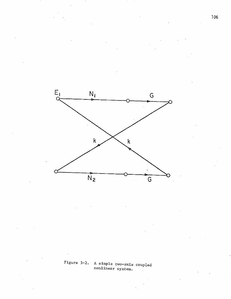
106

E NI G

N2 G

Figure 3-2. A simple two-axis couplednonlinear system.

107

The input signals of the nonlinear elements are written from

Fig. 3-2.

E = kx2 = N2GkE 2 (3-26)

Thus,

EE= N2Gk (3-27)

Also,

E2 = kx = NIGkE1 (3-28)

from which we have

E 11 1 (3-29)

E2 N1Gk

Equations (3-27) and (3-29) are multipled to give

[ N -(3-30)

In order for the system to exhibit self-sustained oscillations, it is

necessary that A = 0 be satisfied, along with any one of Eqs. (3-27),

(3-29), and (3-30). These provide two complex or four real equations

with four unknowns in IE11, IE2 1, w, and 4.

In general, if appropriate initial guesses are available for

IE11, IE21, w, and p, the numerical-iterative method will seek out

108

the solution to the system of nonlinear equations represented by

the equations discussed above. This is useful for the case when

IEIJ = IE2 1 = E, and = 0, since the initial guess for these

solutions is available from the single-axis system solutions.

In the case when IE1I I E2 1 and 1 1 0, a general procedure

is needed to solve the nonlinear equations.

One method of solution is to span the w, 1El, and 1E2 1 space

and plot A (or A - 1) or Eq. (3-25) in magnitude versus phase co-

ordinates, and seek out the A = 0 solutions. These solutions then

become candidates for possible solutions of Eq. (3-27), (3-29) or

(3-30), with the variable parameter C free.

An alternative is to solve Eq. (3-27), (3-29) or (3-30)

first and then use the solution or solutions to check with Eq.

(3-25). Along this direction, a necessary condition for the

existence of limit cycles is given by Eq. (3-30) which is inter-

preted as follows.

Equation (3-30) is written

2 N2(3-31)

Since N2 = N(E2 ) and N1 = N(E1), Eq. (3-31) will be satisfied

if E2 and K/N(E), where K is an arbitrary constant, have the same

magnitude for two different values of E. This means that if the

curves of E2 and K/N(E) are plotted with respect to E, there must

be two intersections between these two curves in order to satisfy

109

Eq. (3-31). Figure 3-3 shows the plots of E2 and Il/NI in db versus

E in db, with N being the describing function of the CMG nonlinearity

with y = 1.38 x 106. It is apparent that these two curves intersect

at at most one point for any K. Therefore, we may conclude that

with the CMG nonlinearity in the system configuration of Fig. 3-2,

self-sustained oscillations of unequal amplitudes cannot occur with

any transfer function G.

Let us define

f = INI (3-32)

1 1h f -IN (3-33)f INI

Also, let

g = logl 0h (3-34)

and

x = log 10E (3-35)

Then, the slope of the curve for I1/NI in Fig. 3-3 is given

by

d 1 dh df dE _ dfdx h df dE dx dE 3-36)

or

d -Eh dE (3-37)dx dE

20

O -

II/NI

-20

SE2

.0 = 1.38x106-40

IN

-60

-so80

-100-160 -140 -120 -100 -80 -60 -40 -20 0 20E(db)

Figure 3-3.

With

f = E2 (3-38)

Eq. (3-36) gives

dg = 2 (3-39)dx

Thus, the necessary condition for Eq. (3-31) to be satisfied is that

the slope of the log1 0 ll/N versus logl 0 E curve exceeds the value 2 at

at least one point. This will ensure two intersections between the

E2 and Il/NI curves.

3-4. A Simplified Multiple-Loop Two-Axis Coupled Nonlinear System

Figure 3-4 shows the signal flow graph of a two-axis coupled

system which is simpler than the LST system and yet still retains

the essential characteristics of the system.

The transfer functions of the system are defined as

G2 2 (3-40)

H = s + 10- 3

These transfer functions and parameters are selected so that

the single-axis system has two limit cycles, one stable and one un-

stable, with y = 1.38 x 106 and To = 0.1 for the CMG nonlinearity.

The determinant of the coupled system is

112

-I

G, H G2GI H

X, El X2 V

-NI -K I

-K,

G, bH G2Y E2 Y2 H

-I

Figure 3-4.

113

2 22 22A = [(1 + HG1G2) - K2G 2] + (N1 + N2 )G1 (1 + HG1G2 - K1G2 )

S 2( 22+ N1N2G1(1 - K1G2) (3-41)

The relationships between El and E2 are determined from the following

equations:

x1 = -N1E1 - G2 x2

x2 = HG1x1 - K1G2y2(3-42)

1 = -N2E2 - G2Y2

Y2 = HG1yl - K1G2x2

Thus,

El _ x1 1 + N2G1 + HG1G2 (3-43)E2 Y1 -K G2(1 + N1G1 )

or

E1 -K1G2(1 + N2G1 )(3-44)

E2 1 + N1G1 + HGIG 2

Again, if we equate Eq. (3-43) to Eq. (3-44), we would get A as in

Eq. (3-41).

From Eqs. (3-43) and (3-44) we have

2 (1 + N2G1 )(l + N2G1 + HG1G2)-E 2 (1 + N1GI )(1 + NIG1 + HG1G2 )

114

The numerical-iterative method was first used to solve for the

conditions of limit cycles for IE1 1 = 1E2 1 given by Eqs. (3-41) and

one of the equations in Eqs. (3-43), (3-44), and (3-45). It turned

out that when IE1 = IE2 1, = 1800; that is, the two sinusoidal

signals at the inputs of N1 and N2 are 180 degrees out of phase.

Using appropriate initial guesses for IE1 = jE2 1, m, and with p =

1800, the numerical-iterative method yielded limit cycle solutions

shown in Fig. 3-5 for various degrees of coupling coefficient K1.

Figure 3-6 shows the numerical iterations for the various values of

K1.

A graphical procedure was carried out for the solution of limit

cycles when E1 I E2, since the numerical-iterative method yielded no

convergent solutions.

Figure 3-7 shows the plots of A of Eq. (3-41) for various com-

binations of {E11 and IE2 1. For limit cycles to exist the plot of A

must go through the (0 db, -180') critical point. Figure 3-7 shows that

the 1E11 = 1E2 1 = 0.9163 x 10-3 locus does go through the critical point.

However, most of the !El{ I IE 2 1 trajectories are far from intersecting

the critical point. Although, it is difficult to span the IE11, IE21space completely, these plots do give indication of possible existence

of unequal-amplitude oscillations.

The other necessary condition that needs to be checked is given

by Eq. (3-45). Let

f = (1 + NG1 + HG1G2 )(1 + NG1 ) (3-46)

Then, for a limit cycle solution, it is necessary that the E2 versus

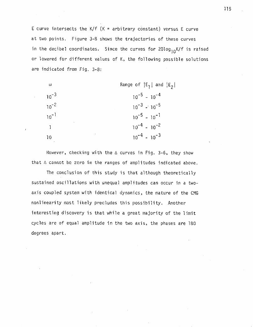
115

E curve intersects the K/f (K = arbitrary constant) versus E curve

at two points. Figure 3-8 shows the trajectories of these curves

in the decibel coordinates. Since the curves for 201og 10K/f is raised

or lowered for different values of K, the following possible solutions

are indicated from Fig. 3-8:

w Range of IE11 and 1E2 1

10- 3 10- 5 - 10- 4

10-2 10-3 10-5

10-1 10-5 - 10-1

1 10- 4 10-2

10 10- - -10 - 3

However, checking with the A curves in Fig. 3-6, they show

that A cannot be zero in the ranges of amplitudes indicated above.

The conclusion of this study is that although theoretically

sustained oscillations with unequal amplitudes can occur in a two-

axis coupled system with identical dynamics, the nature of the CMG

nonlinearity most likely precludes this possibility. Another

interesting discovery is that while a great majority of the limit

cycles are of equal amplitude in the two axis, the phases are 180

degrees apart.

50- K1 9.5x 10-4

40

0 9x104x 30 -

L 20Ix 10-4

IO6

-4-0 10 2x IO0 lK,=o. 10 5

0 2 4 6 8 10 12w (rod/sec) x 163

Figure 3-5.

117

TEST S'YSTEM-NUMERICAL SOLUTION OF DELTAci,,IEl ,E2,THETA)=0.GAMM= 1.300 06 TO 1300 0000D-r 0 TM= .1 . r00000-03 K0 - 1 . 0': 0or' 1l. 0O00 0 OD- 06

ITERATIOFN FRE.GIENCY El E2 F PHA:SE-E10 0.7 000000 iD-02 0 .9c000000l 0 0 .000000-03 0 I.1 I800000IIID 03

1 0.73019411D-02 0 .92994 07D-03 0 .9252 D - i'.19': 1 D 0:32 0. 7279211 D-O2E 0.9214010D-03 0.92127 1-03 01 :8138:3D 033 0.724609'-02 0.9182:3 :' D-0:3 0.916762- 0:: 0 .1 c: 04199 D 03

4 0.72419041'-02 0 .916.5: - - 0.9165417 -0- 0 1-. 009751 03

5 0. 7239953-02 0.9163476D-03 0.91633.1-03 0. 1I:00225D 0:3

6 0.72395 05rD- 02 0 .9162:8:3911-03 0.9162381.-:D- 03 0 . 1800 0691D 03

IND= 1 FRECUENCY= 7.23:940D- 03RADSEC El= 9.16E269D- 04 E2= 9.16268-04THETA= 1.80003D 02' NIT= 6

TEST SYSTEM-NUMERFICAL SOLUTION OF DELTA( U ,E1 E2 ,THETA )=0.GAMMA= 1.3:00 0 06 TO= 1.0IC0O -01 R SM= 1. 0000 TD-0'3 K= 1. I0000 CID-05

ITERATION FREIIUENICY El E2 PHASE-E10 0.7 239395D-02 i 0.91626361- 03 0 .91626:1-03 0 1 ' 00031 031 0.8:372262-02 0 1112_051-02 0.1044::5:_D-02 0i 1 4- 46639D 0:32 0.-922 -02 0 126 073:51-02 0. 124:9201-02 0 1::546D 0:3 0.64:-9651D-02 0. 1 0203441-02 0 .957651 ': 11- 0:3 0 1746, 1D 034 0.7 0 541 92-02 0. 1 03:2 0 -02 0.05:0C . I C :4D- 02 0 17 1 419 035 0.751::3007D- 02 0 1097541- 02 0 . 110112-02 0 .1737:;5D 036 0.7793'- 0 1130505-02 . 113'4'D-02 0 . 1796 059 0:-37 0 .7::691 07D -02 0 .1392D- 02 0.11 39 15-0 0. 1799691 03:2: 0.73776 078: - 02 0 .1 14 0722D-02 .1 4 0.1 1 4 072 :- 0 - ' .1: 0010 03

9 0.7876270D-02 0 . 114 074:D- 1-02 0. 114 07415:- O 0. 1800019D 0:3

IND= I FREQEN'CY= 7.:7627 D- 03RAD''/SEC El= 1.14075D-03 E= 1.14075D-03THETA= 1 .80002 02 NIT= 9

Figure 3-6a.

118TEST SYSTEM-NUMERICAL SOLUTION OF lELTA(W,EI,E2,THETAW=0.GAMMA= 1.382000D 06 TO= 1.00000D-01 A= 1.0000-03 KI= 1.000001D-04

ITERATION FREQUENCY El ES PHASE-E1

0 0.994100D-02 0.2520000-02 0.2520000D-02 0.1800000D 0:3

1 0.9941336D-02 0.2520555D-02 0.2520555D-02 O. 01:800019D 03

2 0.9941336D-02 0.252 0555D- 20555D-02 0.1800019 03

IND= 1 FRE!UENCY= 9.94134D-O3RAD/SEC El= 2.52056D-03 E2= 2.52056D-0:3

THETA= 1.80002D 02 NIT= 2

TEST SYSTEM-NUMERICAL SOLUTION OF DELTI(WI,E1,E2,THETA)=0.GAMMA.= 1.38:00D 06 TO- 1.0000D-01 ASM= 1.0000oD-03 Kl= 2.000001-04

ITERATION FREQCUENCY El E2 PHASE-E1

0 0.99413361-02 0.2520555-02 0.25205551- 0 .252 0 -02 0.1800019D 03

1 0.388266;ID-02 0.3492311'-02 0.3775372D-0 0 . 1787370D 03

2 0.9573039D-02 0.3637139D-02 0.3846694D-02 0.1793218D 0:3

3 0.1012638- 01 0.3725995D-02 0.3774828D-02 0.1797817D 0:3

4 0. 1 036430D-01 0.3744250D-02 0.37496021- 02 0. 1799755D 03

5 0.1039656D-01 0.3746356D-02 0.37464 05'- 02 0.1800016D 03

6 0. 1039692-01 0.3746376D-02 0.3746375D-02 0.18000119D 0:3

IND= 1 FREQUECY 1 . 03969D- 02RADSEC El= 3.746:38D-03 E= 3.74638D-0:3

THETA= 1.80002D 02 NIT= 6

TEST SYSTEM-NUMERICAL SOLUTION OF TIELTR(W,E1,E2THETA )=0.

GAMMA= 1.38000D 06 TO= 1.'0000D-01 ASM= 1. 0000OD-03 K= 4.00000D-04

ITERATION FREQUENCY El E2 PHASE-El

0 0.1039691'-01 0.3746375D- 02 0.3746 375 - 02 0.1800019D 0:3

1 0.5863165D-02 0.7227177D-02 0.745150I1-02 0.1768248D 0:3

2 0.6955595D-02 0 .6060'971D-02 0 .::70 78D- 02 ' . 1773450D 03

3 0.8078298- 02 0 .6229025D-02 0.7205775D-02 0.1785639IF 0:34 0.9031302D-02 0.6315208' -02 0.672496D- 02 0. 1793910D 03

5 0.9617574D-02 0.6363023D-02 0.64832011-02 0.17984921 03

6 0.900658:D1-02 0.6409813D-02 0.641699:8:D-02 0. 1799869D 03

7 0.9::821735D- 02 0.6409441D-02 0.64 09438D-02 0. 1800018D 03

8 0.9821825D-02 0.6409420D-02 0.6409420D-02 0.1800019D 03

IND= 1 FREQUENCY= 9.82182D- ORADYDSEC El= 6.40942D-03 E2= 6.40942P-0-3THETA= 1.80002D 02 NIT= 8

TEST SYSTEM-NUMERICFAL SOLUTION OF DELTAII ElsE2,THETA=O.GAFMMA= 1.38000D 06 TO= l.00000D-01 ASM= 1.0000D-03 Kl= 6.00000- 04

ITERATION FREQUENCY El E2 PHASE-El

0 0.9212'5D- 02 0.640942' O- 0 .649420D-02 L.18 0001 9D 03

1 0.5735355D-02 0.114492:1-01 0.11604'52D-01 0 17.77600' 03

2 0.6465793 -02 0.1 071898D-01 0.1248778D-01 0 .1782281D 0:3

3 0.7323528D-02' 0.1057956D-01 0.111982'5D-01 0.1792237D 03

4 0.7914920D-02 0.1040805D-01 0.1059804D-01 0.1797632D 03

5 0.:16241:8-02 0.1034690D-01 0.1036832D-01 0.1799723D 0:3

6 0.819:8133D-02 0.1 033763D-01 0.103377' :-01 0.1800 015D 03

7 0.81985881-02 0. Iu33746-01 0.1033746D-01 0.1800019D 03

IND= 1 FREQUENCY= 8.19858D-03RAD'SEC El= 1.03375D-02 E2= 1.033751-02THETA= 1.80002D 02 NIT= 7

Figure 3-6b.

119TET Y:'STEM-NUMEPICAL SOLUTION OF DELTFAW,EiE,E2,THETA)=0.GARMMA= 1.3:001' 06. TO= 1.O000ODl-01 A:M= 1.0000OD-03 Ki= s.00000D-04

ITERATION FREQUENCY El E2 PHFASE-E 10 0.8198585D-02 0. 1033746D-01 0. 1 033746D-01 0.1800019D 03

1 0.342245D- 02 0.18:392741-01 0.2190817D-01 0.175351ID 03

2 0.3121926D-02 0.272071D-01 0.3050192D- 01 0.1753942D 0:33 0.3694573D-02 0.2440467D-01 0.2737973D-01 0.1771812D 0:34 0.4333109D-02 0.2224205D-01 0.2334315D-01 0.1784748D 035 0.490'505D-02 0.2043765D-01 0.2107548D-01 0. 1792209D 03

6 0.5335999D-02 0.194T21 -D-01 0.1963290D-01 0.1797269D 03

7 0.5546392--02 0. 19970ID-01 0.190313611-01 0.1799537D 03

8 0.5590206D-02 0. 1891363D-01 0. 18914 180D-01 0. 18:30006D 03

9 0.5591465D-02 0.1891121D-01 0.1891118D-01 0.1800019D 03

10 0.5591450D-02 0.1891123D-01 0.1891123D-01 0.1800019D 03

IND= 1 FREQUENCY= 5.59145D-03RFAD/SEC El= 1.89112D-02 E2= 1.891121-02THETA= 1.80001D 02 NIT= 10

TEST SYSTEM-NUMERICAL :SOLUTION OF DELTA(Wi,E1,E2,THETA)=0.GAMMA= 1.38000D 06 TO= 1.000001-01 SM= 1.0000'0D-03 Kl= 8.50000D-04

ITERATION FREQUENCY El E2 PHASE-El0 0.5591451D-02 0.1891123D-01 0.1891123D-01 0.1800019D 031 0.4560251D-02 0.2399517D-01 0.2316868D-01 0.1797862D 0:3

2 0.4661299D-02 0.2368992D-01 0.2378736D-01 0.1799267D 033 0.4713075D-02 0.2354609D-01 0.2354633D-01 0.1799992D 034 0.47154 471 53D-02 0.2353:809D-01 0.2353802D-01 0.1800019D 0:35 0.4715421D-02 0.2353818D-01 0.235318 :D- 01 0.1800019D 03

IND= 1 FREQUENCY= 4.71542D-03RAD/SEC El= 2.35382D-02 E2= 2.35382D-02THETA= 1.80002D 02 NIT= 5

TEST SYSTEM-NUMERICAL S:OLUTION OF DELTA (I ElE2,THETA)=0.GFMM= 1.38000D 06 TC= 1.0000D-01 A:M= 1.O0000o-03 Kl= 9.00000-04

ITERATION FREQUENCY El E2 PHASE-El0 0.4715422D-02 0.23'53818 D-01 0.2353818D-01 0.1:00019 031 0.3485092D-02 0.3142799D-01 0.3107595D-01 0.1791651D 032 0.3532983D-02 0.3254668D-01 0.328058.6D-01 0.1797728D 033 0.365917 0-02 0.3 172735D-01 0.3173334D-01 0.1799660D 0:34 0.368481OD-02 0.3155989D-01 0.3155995D-01 0.1 00010D 035 0.3685423D-02 0.3155622D-01 0.3155619D-01 0.1800019D 03

6 0.3685410D-02 0.3155631D-01 0.31556311-01 0.1 :80O0019D 03

IND= 1 FREQUENCY= 3.685411D-03RAD/'SEC El= 3.15563D-02 E2= 3.15563D-02THETA= 1.80002D1 02 NIT= 6

TEST SYSTEM-HUMERICOL SOLUTION OF DELTF A EIE1 E2,THETA :=0.GAMMA= 1.38000D 06 TO= 1. 0000D-01 ASM= 10000D-63 Kl= 9.50000D-04

ITERATION FREQUENCY El E2 PHS-E-E 10 0.368'5410D-02 0.3155630D-01 0.21556301-01 0.180 0019D 03

1 0.1976666D-02 0 .415936D-01 0.55:82929D-01 0.1726228D 03

2 0.16574161D-02 0.6596966D-01 0.7001921D-01 0.1770600D 03

3 0.1800327D-02 0 .65918 771-01 0.6669853D-01 0.1790101D 03

4 0.2020104D-02 0.5954712D-01 0.'5879754D-01 0.179528D 03

'5 0.2196704D-02 0.5491415D-01 0.548405D-01 0.1797066D 03 -:

6 0.232 3 2 6D-02 0.5217919D-01 0.5216096D-01 0.179:88 91 03

7 0.23::: 15::86D-02 0.l 510730:D-01 0.5107025D-01 0.1799836D 038 0.239155::D-02 0.5089335D-01 0.50892601D-01 0.1800019D 039 0.2391499D-02 0. 509476D-01 0.5089477D-01 0.1800019D 03

IND= I FRPEUENCY= 2.39150D-03 'ADSEC El= 5.089471D-02 E2= 5.08947D-02THETA = 1.830002D 02 NIT= 9

Figure 3-6c.

300

250 -(5,5) (3,5

(n,m) represents

IE1 IE 2 1) = (10-10-m) 200

u 150w

LLJ (4,4)100-

1,2)(1,2) (3,3

2,2)

2,2)E E=E2 0.9163xlO

-120 -60 -360 -300 -240 -180 -120DEGREES

Fiure 3-7.

121

20 log o10 E2

20-

20 logo 100 )

2= 102 W = 1-20 -

-40 - -

-60

-100-

-120-

-140- =7 -

-160-

-180-

-200-

-220 -

-240 I I I I I-160 -140. -120 -100 -80 -60 -40 -20 0 20

20 logloE (db)

122

DISTRIBUTION LIST

Final Report 1-75 NAS8-29853

AS21D 5

EDl2/S/Seltzer 10

ED11/G/Nurre 1

EM34 1

ATOI 1