research paper condition assessment of building façades
TRANSCRIPT
RESEARCH PAPER Condition assessment of building façades based on hazard for people
Félix Ruiza1, Antonio Aguadoa, Carles Serratb and Joan R. Casasa aBarcelona School of Civil Engineering (Department of Civil and Environmental
Engineering), bBarcelona School of Building Construction (Institute of Statistics and Mathematics
Applied to the Building Construction), Technical University of Catalonia-BarcelonaTECH
To make periodic inspections of the buildings is useful to quantify the extent to which deficiencies are severe or not, in order to facilitate decision making and prioritize interventions. In previous works by the authors is proposed a scale of gravity of damages in buildings, with the aim of being of widespread and of common use among professionals. This scale is applied through the direct assignment methodology (DA), based on the generic definitions of each degree. It is demonstrated and characterized the existence of certain level of variability among technicians, when assigning gravity values using DA methodology, due to the fuzzy condition of the attribute to be evaluated. The main goal of this paper is to propose a methodology to assign values of gravity, based on hazard for people of detachments from the façade, by using measurable parameters and mathematical functions. The final objective is to reduce the level of variability among inspectors when assessing the condition state of a building façade. The proposed methodology is named System of Evaluation of Façades (SEF). The methodology can be also extended to the assessment of other building systems as structures or roofs and other type of infrastructures. Keywords: scale, degree of gravity, damages, façade, indicator, algorithm, condition state. 1. Introduction
Damage diagnosis is undoubtedly one of the biggest challenges for engineering in the 21st century (Pardo and Aguado 2017). In civil engineering, as in humans, structural damage can be understood as the structure’s failure to fight off internal or external elements attacking it. Thus, the diagnosis must be understood as a systematic analysis of physical signs observed at the construction.
Focusing the target in building construction, the interest in the evolution of the building and infrastructure stocks has been evolving during time, in some cases closely linked to the
1 Corresponding autor: Email: [email protected] Other autors: Email: [email protected] // [email protected] // [email protected]
sustainable development debate (Kohler and Yang 2007). The topic of maintenance optimisation has been a focus of research interest since some time ago (Mazzuchi and René 2012). A central issue is the buildings end of life. Lifetables of classical population dynamics (Klein and Moeschberger 2003) can be used for estimating the end of life of a sample of building and infrastructure stocks (Herz 1998; Schiller 2007). In the same way, there are several authors who investigated construction defects, usually focused on failures in buildings due to lack of maintenance, design and construction errors, execution failure, material defect, inappropriate use, etc. (Frangopol 2011; Gibert 2016). Some of these defects are: humidity, defects in roofs, in natural stone coverings (Neto and de Brito 2012), in ceramic façade claddings (Silvestre and de Brito 2011), in masonry (Li et al. 2017), damage on the envelope of buildings (Rodrigues et al. 2011), damage in load-bearing rammed earth walls (Ruiz 2013), problems in the subsoil (Díaz et al. 2015), among others.
On the other hand, the rapid industrialization and population migration of the last 30 years in many parts of the world, has led to fast growing urbanization, doubling the building and partially the infrastructure stocks in very short periods (20-30 years), and this may happen more than once a century (Yang 2006). The growth rate is very high and it is not always known how well these stocks are constructed. At present, about 50% of the investments in construction are related to existing structures (Sykora et al. 2017). In this context, the crucial indicator is the state of degradation of the different components of the stock and an objective indicator of this condition state (Kohler and Yang 2007). In the same way, various asset management tools have been introduced to help asset managers in the difficult decisions regarding how and when to repair/replace their existing building stock cost-effectively (Elhakeem and Hegazy 2012; Kobayashi and Kaito 2017).
It is demonstrated the importance of performing preventive maintenance in buildings in order to prevent their degradation and the appearance of severe malfunctions (BRIME 1999). In the framework of maintenance, to make periodic inspections of buildings is useful to quantify the extent to which deficiencies are severe or not, in order to facilitate decision making and prioritize interventions (Flourentzou et al. 2000; Serrat and Gibert 2011). Efficient and effective inspection and maintenance planning can be made based on an optimization process (Miyamoto et al. 2000; Kim and Frangopol 2017). The economically-based approach wants to optimize the available budgets in the basis of medium and long-term efficiency. However, an economic approach only, can not always guarantee the human safety and minimize the risk associated to the failure of some building elements. Such is the case of the components of the building façades, where the detachment of some elements (coating, plaster, stone, bricks…) may derive on the injury or death of people below. Therefore, apart from the economic optimization, an assessment of building façades based on this risk seems worth to be investigated.
On the other hand, it is important to highlight that, currently, there are many scales used to assess the grade of severity of damage (or condition state index) of the constructive elements in buildings. There is no consensus and these scales are different, with different number of degrees and metrics, according to the study to which they belong (Ruiz et al. 2019). In Ruiz (2014a) is proposed a scale of gravity of damages in buildings, with the aim of being of widespread and of common use among professionals. This scale is applied through the direct assignment methodology (DA), based on the generic definitions of each degree. In Ruiz (2014a) and in Ruiz et al. (2019) is also demonstrated and characterized the existence of certain level of variability among technicians, when assigning gravity values using DA methodology, due to the fuzzy condition of the attribute to be evaluated. Therefore, the main objective of this paper is to make an alternative proposal to the direct
assignment method (DA) to evaluate the degree of gravity in building façades, based on objectively measurable parameters, in order to reduce as much as possible the degree of variability when assigning a certain degree of gravity G. More specifically, the proposal consists in the appropriate selection of objective and measurable indicators and the associated calculation methods. The degree of gravity is quantitatively defined by considering the risk to people of façade elements falling down. The proposed methodology has been derived in the specific case of building façades, and it is named System of Evaluation of Façades (SEF). However, it is important to highlight that the techniques and tools proposed in this methodology can be used in future lines of research, applying the methodology to evaluate structures, roofs, etc., and also in other type of infrastructures.
In order to highlight the topic, below some real examples of detachments of façades with human losses are described. Although when a detachment of façade occurs, the probability to impact on a person is low (it depends on several parameters as if the street is crowed or not, etc.), it is non zero. As an example, in the center of the city of Barcelona three people died due to impacts of detachments from façades in a short period of time. Specifically, on October 2nd of 1996, a three year old girl died when a ceramic tile on the seventh floor of a building on Roger de Flor Street fell on her. On May 6th of 1997, a 37 year old woman died when she was hit by a stone element from a façade on Trafalgar Street when she was accompanying her son to school. And on February 22nd of 1998, a 56 year old German tourist died when an artificial stone element of the façade, weighing 5kg hit her on the head from the 3rd floor while she was walking along the Passeig de Gràcia (Ruiz 2014a). In order to explain a more recent case, on August 20th of 2014, in Argüelles neighborhood in Madrid, the detachment of part of the coating of a balcony in a 8th floor impacted over two young men who were sitting on the terrace of a bar, on the street. The impact caused the death of one and mild injuries on the other (Ruiz 2014b).
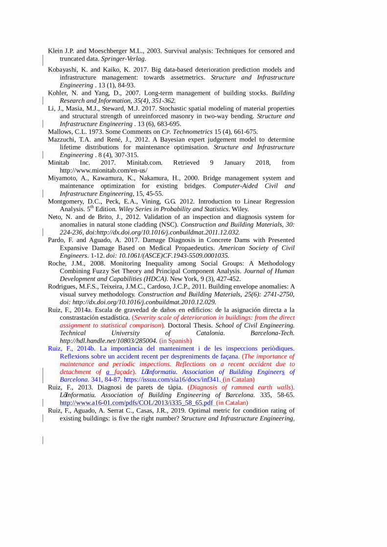
2. General Methodology The proposed methodology is named System of Evaluation of Façades (SEF), and it is composed of two parts: graphical and numerical. The graphical part shows the façade and the zones that are delimited, based on the existing deteriorations and on the characteristics of the materials and the building elements present in the façade. In the numerical part, once the different façade data are obtained from the graphical part, the indicators are calculated to determine the degree of gravity of each zone j of the façade, Gj, with the lowest degree of variability. Figure 1 presents a scheme of the proposed SEF methodology.
Figure 1. Outline of the methodology SEF (System of Evaluation of Façades)
For the development of the methodology, seven cases of facades with different deteriorations, construction typologies and materials have been selected. As shown in Figure 1, the numerical part focuses on the calculation of two indicators as a measure of the impact of falling elements and the probability of detachment, respectively. In terms of impact energy, physical variables of degraded areas are considered, and a statistical study is carried out with regard to the probability of detachment.
2.1. Methodology SEF: Graphical part The graphical part has the following two main objectives:
· graphical representation of the façade · delimitation of zones where a deterioration is detected
The methodology consists of two main phases: obtaining the data, and representation of
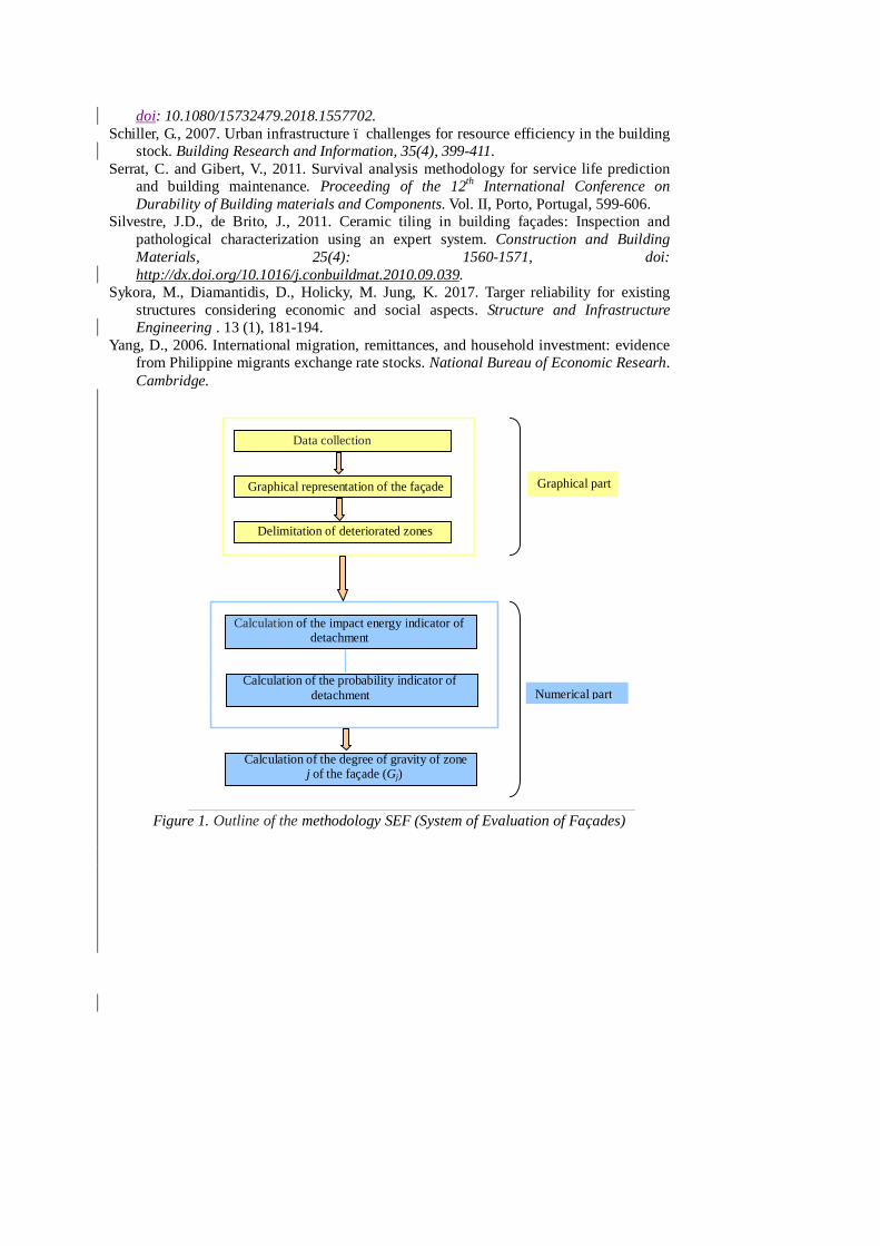
the obtained data. The following sections explain this methodology. Data collection The first step is to make the visual inspection of the façade, as well as taking sufficient data (length, height, etc.) to be able to draw it as accurately as possible. The inspection is carried out from the outside, also making photographs of the façade, both general and detail views. In order to be able to observe certain zones that are not seen in sufficient detail, binoculars are used, especially in zones where there are deteriorations. The entire façade is observed, including all elements such as cantilevers, cornices, cladding, ornamental elements, openings, handrails and balustrades, etc. In order to facilitate the work of the inspector, is useful to have a sheet to standardize the data collection. This sheet should be easy to application and further interpretation and, at the same time, the main characteristics of the façade and its deteriorations should be included. An example of the sheet is presented in Table 9. A sheet must be obtained for each façade of the building and must include the graphic representation of the façade, where the different existing damages are delimited and numbered. Graphical representation of the façade After gathering the data, the next step is to make the graphical representation of the façade, for which the photographs and main dimensions of the façade are used. The combination of the drawing and the photographs is performed to obtain the necessary set of information, as shown in Figure 2. Alternative tools, such as photogrammetry, can also be used. The graphical representation of the facade is done with the corresponding software, what allows to calculate the affected surface.
Figure 2. Example of image and graphical representation of façade
Delimitation of deteriorated zones
The marking of deteriorated zones is carried out with the general criterion that each delimited zone has homogeneous characteristics in terms of the type of material, type of construction and existing deterioration. The data of the different delimited deteriorated zones are compiled in a table on the same drawing sheet, as presented in Table 1. This table
is exported to a spreadsheet where subsequent calculations are made, which are explained later.
Table 1. Delimited deteriorated zones of façade The following descriptions apply to the columns in Table 1:
- ID: identification number of each delimited zone (correlative). - Surface (S): surface in m2 of the delimited zone.
- h: height in m of the geometric center of the delimited zone, taken from the level 0
of the façade.
- Thickness (T): thickness in m of the material of the delimited zone.
- Material (M): type of material in the delimited zone (whether it is cement mortar, brick factory, etc.).
- ls: surface correction factor, per unit, for cases in which the delimited zone has
parts that have already been detached, thus adjusting the surface delimited in the drawing to the part that is actually deteriorated and presents a risk of detachment.
- Corrected surface (CS): surface in m2 of the delimited zone to which the surface
correction factor (ls) has been applied, surface corrected = ls · surface.
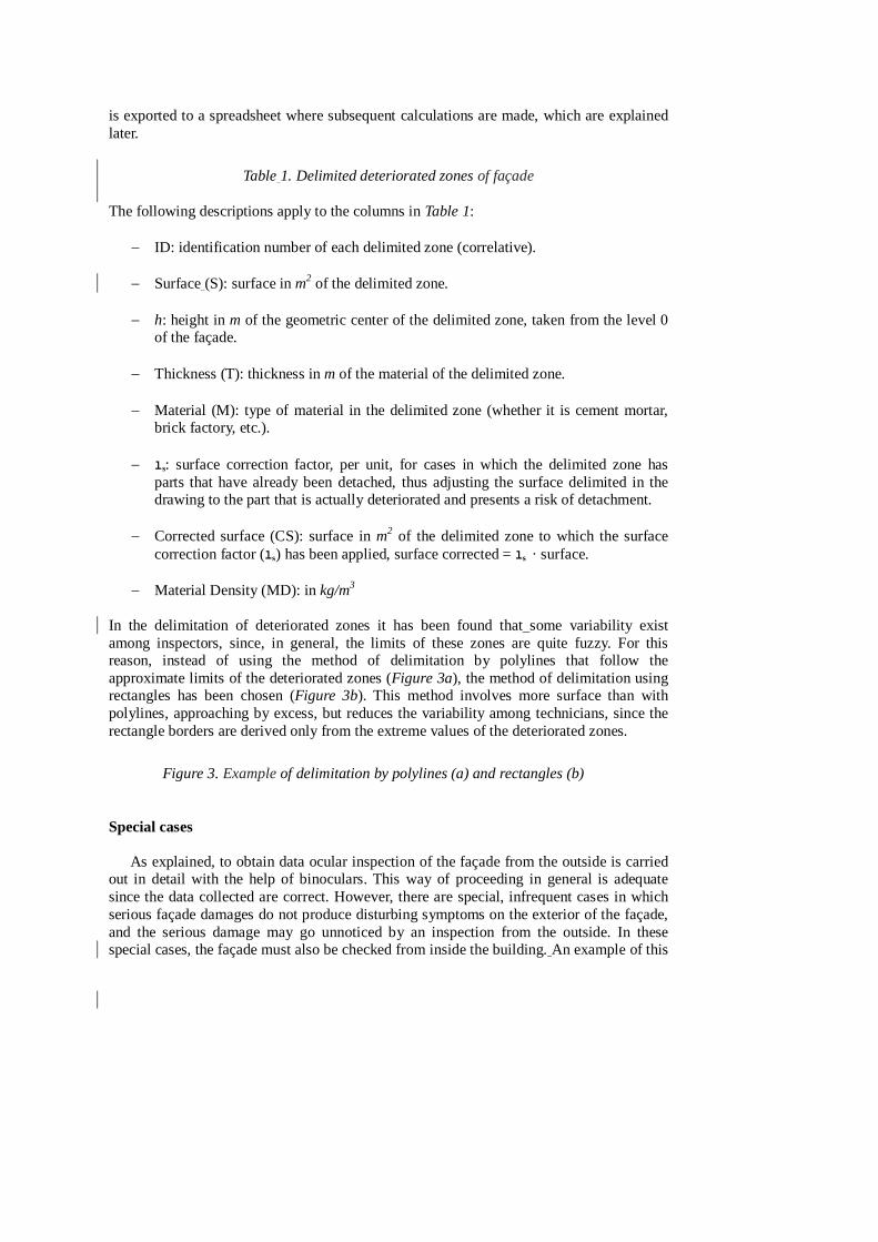
- Material Density (MD): in kg/m3 In the delimitation of deteriorated zones it has been found that some variability exist among inspectors, since, in general, the limits of these zones are quite fuzzy. For this reason, instead of using the method of delimitation by polylines that follow the approximate limits of the deteriorated zones (Figure 3a), the method of delimitation using rectangles has been chosen (Figure 3b). This method involves more surface than with polylines, approaching by excess, but reduces the variability among technicians, since the rectangle borders are derived only from the extreme values of the deteriorated zones.
Figure 3. Example of delimitation by polylines (a) and rectangles (b)
Special cases
As explained, to obtain data ocular inspection of the façade from the outside is carried out in detail with the help of binoculars. This way of proceeding in general is adequate since the data collected are correct. However, there are special, infrequent cases in which serious façade damages do not produce disturbing symptoms on the exterior of the façade, and the serious damage may go unnoticed by an inspection from the outside. In these special cases, the façade must also be checked from inside the building. An example of this
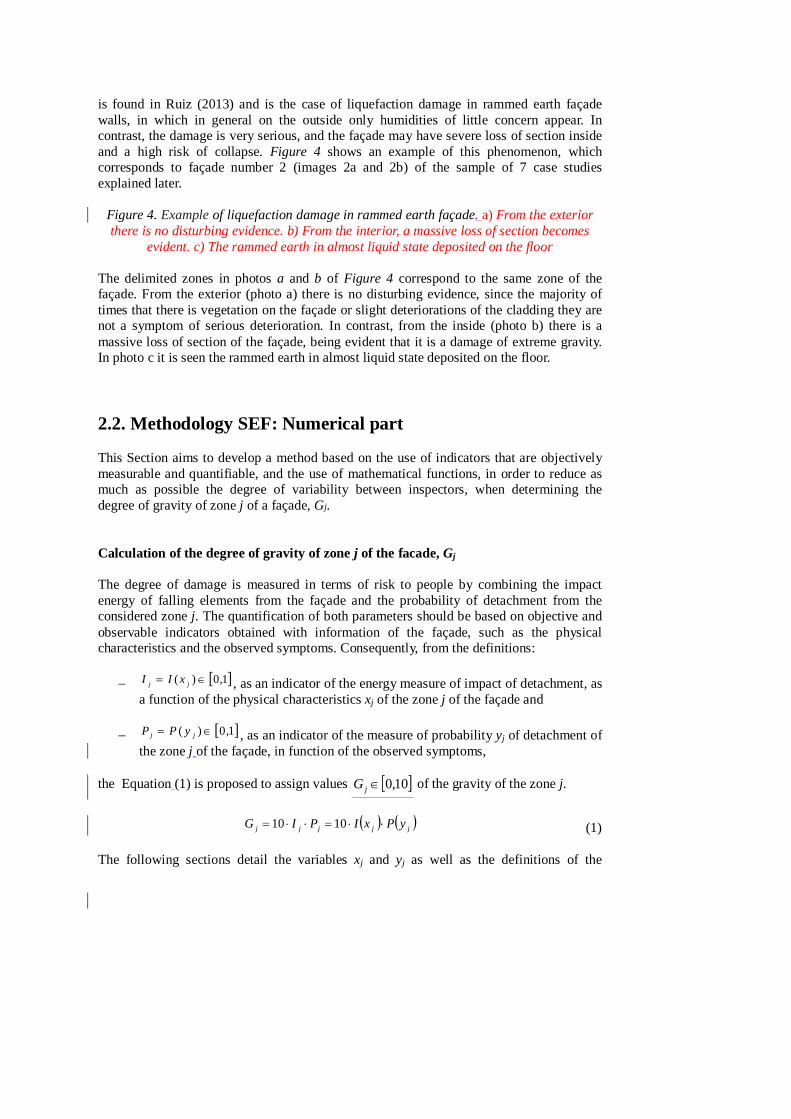
is found in Ruiz (2013) and is the case of liquefaction damage in rammed earth façade walls, in which in general on the outside only humidities of little concern appear. In contrast, the damage is very serious, and the façade may have severe loss of section inside and a high risk of collapse. Figure 4 shows an example of this phenomenon, which corresponds to façade number 2 (images 2a and 2b) of the sample of 7 case studies explained later.
Figure 4. Example of liquefaction damage in rammed earth façade. a) From the exterior there is no disturbing evidence. b) From the interior, a massive loss of section becomes
evident. c) The rammed earth in almost liquid state deposited on the floor
The delimited zones in photos a and b of Figure 4 correspond to the same zone of the façade. From the exterior (photo a) there is no disturbing evidence, since the majority of times that there is vegetation on the façade or slight deteriorations of the cladding they are not a symptom of serious deterioration. In contrast, from the inside (photo b) there is a massive loss of section of the façade, being evident that it is a damage of extreme gravity. In photo c it is seen the rammed earth in almost liquid state deposited on the floor. 2.2. Methodology SEF: Numerical part This Section aims to develop a method based on the use of indicators that are objectively measurable and quantifiable, and the use of mathematical functions, in order to reduce as much as possible the degree of variability between inspectors, when determining the degree of gravity of zone j of a façade, Gj.
Calculation of the degree of gravity of zone j of the facade, Gj The degree of damage is measured in terms of risk to people by combining the impact energy of falling elements from the façade and the probability of detachment from the considered zone j. The quantification of both parameters should be based on objective and observable indicators obtained with information of the façade, such as the physical characteristics and the observed symptoms. Consequently, from the definitions:
- [ ]1,0)( Î= jj xII , as an indicator of the energy measure of impact of detachment, as a function of the physical characteristics xj of the zone j of the façade and
- [ ]1,0)( Î= jj yPP , as an indicator of the measure of probability yj of detachment of
the zone j of the façade, in function of the observed symptoms,
the Equation (1) is proposed to assign values [ ]10,0ÎjG of the gravity of the zone j.
( ) ( )jjjjj yPxIPIG ××=××= 1010 (1)
The following sections detail the variables xj and yj as well as the definitions of the
associated I and P value functions.
Indicator for the measurement of the impact energy of the detachment The impact energy oh the detachment of zone j is obtained from the physical concepts of
momentum ( vmp ×= ), force ( amF ×= = dtdp
) and work ( dFW ×= ), with dimensions,
[ ]22 -TML and unit in the international system of Joule (J)), and is given by the Equation (2).
ghmW jjj ××= (2)
where
- =jm mass of the considered zone j
- =jh height of the geometric center of the considered zone j
- g = acceleration of gravity ( 28,9 smcteg == ) In order to assess the damage caused by the impact of a detached element of façade, it is necessary that in the Equation (2) the surface of the zone considered Sj is also involved. This is so because the same energy value may have associated cases with clearly different impact characteristics, as a function of Sj, due to the inverse relation existing in the surface-impact binomial (Ruiz, 2014a). The measure of the impact energy of detachment is shown in the Equation (3).
j
jjj S
ghmx
××= (en J/ 2m ) (3)
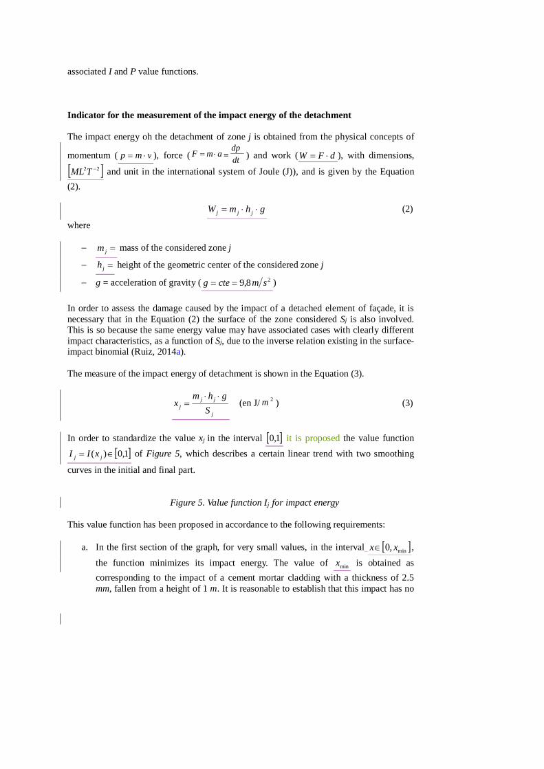
In order to standardize the value xj in the interval [ ]1,0 it is proposed the value function
[ ]1,0)( Î= jj xII of Figure 5, which describes a certain linear trend with two smoothing
curves in the initial and final part.
Figure 5. Value function Ij for impact energy
This value function has been proposed in accordance to the following requirements:
a. In the first section of the graph, for very small values, in the interval [ ]min,0 xxÎ ,
the function minimizes its impact energy. The value of minx is obtained as corresponding to the impact of a cement mortar cladding with a thickness of 2.5 mm, fallen from a height of 1 m. It is reasonable to establish that this impact has no
effect on the human being. Considering a specific weight of the cement mortar cladding 3/2 mTn=g , a value minx = 50 J/ 2m is obtained (Tn means tones).
The function jI is maximum from a given value maxx . It is considered that from a
certain point the damage that can be caused is important enough to continue maintaining the maximum value ( =jI 1). A study in the field of Safety and
Hygiene has been considered applicable (Centurion Safety Products Ltd., 2009). This study is based on the Shock Absorption Test according to UNE-EN 397: 1995, which states that the safety helmets used by workers at site must resist an impact of a mass of 5 kg falling from a height of 1 m. Based on that, with data of m = 5 kg and h = 1 m, it is obtained xmax = 5.000 J/ (considering that the surface of the mass is 10 cm x 10 cm) as the saturation value of the impact energy measure. In fact, if for impact forces higher than this, a construction helmet can fracture, it is suitable to consider that if this impact directly affects a human being (logically not protected by a helmet) it would cause damage severe or very severe.
b. The function has a point of zero curvature at a certain point ix . To determine the
inflection point it has been considered the data of m = 2 kg and h = 1 m, for which is obtained ix = 2.000 J/ 2m (under the same experimental conditions of
requirement b, considering that the surface of the mass is 10 cm x 10 cm).
c. The function is non-decreasing in [ ]min max,x x
This type of function is obtained by the tetraparametrized sigmoid (Alarcón et al. 2011)
( )( )min
min max( ; , , , ) 1 k x xif x x x x e
a
a g - -= - (4) where,
- minx : lower bound - maxx : upper bound - ix : abscissa of the inflection point - α : shape factor, α > 1
with
( )´min
( 1)
i
kx x a
aa
-=
- (5)
( )( )max min1
1 k x xea
g-
- -= - (6)
and
minx = 50 J/m2 , maxx = 5.000 J/m2 , ix = 2.000 J/m2 , a = 2.
Indicator for the measurement of the probability of detachment In this case a categorical ordinal variable yj must be measured (the probability that a detachment occurs), not a continuous variable (mass, height, area) as in the previous indicator Ij. It is a variable that reflects the estimation by the technician of the probability of detachment. Given the categorical nature of the variable, it has been considered appropriate to classify the measure of the probability of detachment based on 5 different degrees: very low (y = 0), low (y = 1), medium (y = 2), high (y = 3) and very high (y = 4). The number of five degrees is based on the study presented in Ruiz et al. (2019), where the direct assignment method is used in the field of assessing the gravity of damage to buildings. This measure yj is consequence of the identification of certain identifiable symptoms in the façade. In the next section a statistical study is developed with the aim of characterizing which are these symptoms and their relationship with the assignment of a probability measure.
About the selection of a metric of five degrees it should be highlighted that in Ruiz et al. (2019), the most suitable metric (number of degrees) of the scale is estimated following a methodological process (including experimental and calculation processes), and not based in the opinion of the authors of the scale, as happens in others scales. It should be added that there are many different scales in the scope of condition state of buildings, with different metrics (different number of degrees). So, in this scope there are scales with 3, 4, 5, 6, 7, 8, 9, 10, 11, 30, 40, 100, etc., degrees (Ruiz et al. 2019).
Multivariate analysis for the estimation of the value yj For the estimation of the values yj from identifiable symptoms in the façade, a multivariate analysis is carried out with data from a sample of images of façade zones, with different levels of deterioration and representative of the study population. For each image, the corresponding symptomatology is available and the detachment probability measure is assigned based on the average value of direct assignment by a team of experts. In order to facilitate the notation in the statistical methodology, in the following the subscript j will be omitted, being y the variable of interest, meaning by omission the zone j of the façade. Figure 6 shows a diagram of the aforementioned methodology.
Figure 6. Diagram of the methodology for the estimation of the y value
The following explains each of the steps in the aforementioned methodology.
Selection of Images of Façades In each of the images of selected façades, a specific zone has been delimited, which is what the expert must evaluate with respect to the probability of detachment. The criteria for selecting images are the following:
1. The selected images cover a wide spectrum of façades and damages. The images are selected in one side from the point of view of the probability of detachment, having zones of selected façades in perfect state of conservation, with very low risk of detachment (y = 0), to areas of extremely deteriorated façades with very high risk of detachment (y = 4), passing through intermediate cases (0 < y < 4). The representativeness of the selected images is also from the point of view of construction type and materials, including cantilevers, cornices, ornamental elements, mortar coatings, façade base material, etc., with variability of materials.
2. The number of selected images is sufficiently high for its adequate statistical
analysis. In order to make the statistical analysis as balanced as possible, a similar number of images have been selected for each value of y (approximately 40 images for each value of y). Specifically, the sample size of the set is 197 images.
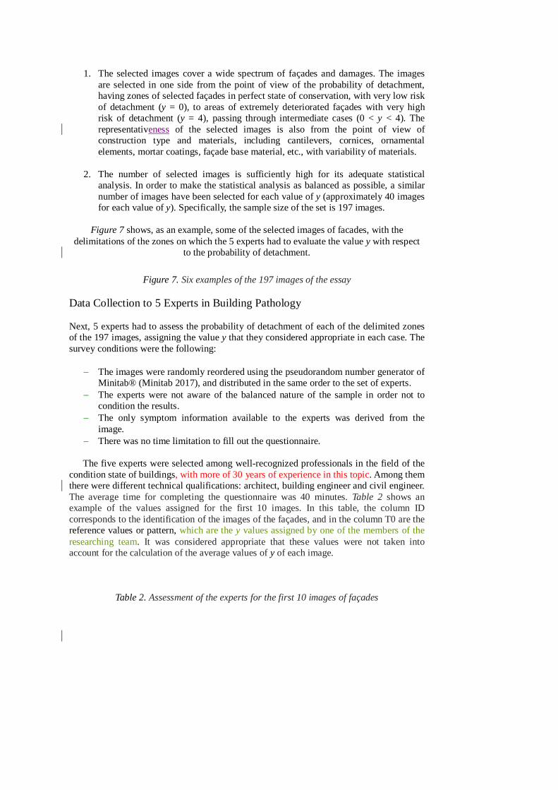
Figure 7 shows, as an example, some of the selected images of facades, with the delimitations of the zones on which the 5 experts had to evaluate the value y with respect
to the probability of detachment.
Figure 7. Six examples of the 197 images of the essay Data Collection to 5 Experts in Building Pathology Next, 5 experts had to assess the probability of detachment of each of the delimited zones of the 197 images, assigning the value y that they considered appropriate in each case. The survey conditions were the following:
- The images were randomly reordered using the pseudorandom number generator of
Minitab® (Minitab 2017), and distributed in the same order to the set of experts. - The experts were not aware of the balanced nature of the sample in order not to
condition the results. - The only symptom information available to the experts was derived from the
image. - There was no time limitation to fill out the questionnaire.
The five experts were selected among well-recognized professionals in the field of the
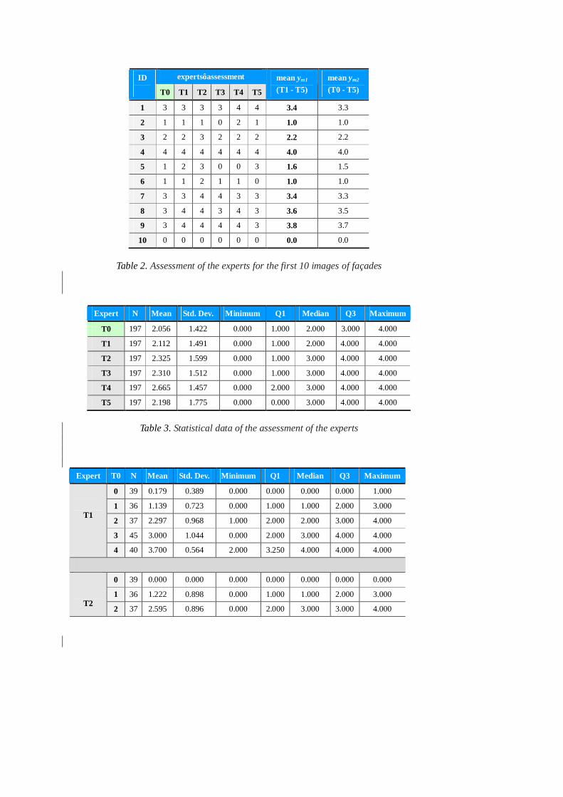
condition state of buildings, with more of 30 years of experience in this topic. Among them there were different technical qualifications: architect, building engineer and civil engineer. The average time for completing the questionnaire was 40 minutes. Table 2 shows an example of the values assigned for the first 10 images. In this table, the column ID corresponds to the identification of the images of the façades, and in the column T0 are the reference values or pattern, which are the y values assigned by one of the members of the researching team. It was considered appropriate that these values were not taken into account for the calculation of the average values of y of each image.
Table 2. Assessment of the experts for the first 10 images of façades
Thus, the values that have been considered for the subsequent steps of the method are those that appear in the table as ym1, which encompass the values of columns T1 to T5, corresponding to the y values assigned by the 5 experts referred to. In any case it is verified that these values ym1 hardly vary from the averages when the reference values or pattern are included, as presented in the table as ym2. Analogously, the values ym1 vary little with respect to reference values or pattern (which appear in the T0 column).
Table 3 presents the main global statistical data (summary and distribution) of the experts assessment, where N is the number of assessed images, and Q1 and Q3 are the first and third quartiles, respectively. It is observed in this table that the arithmetic means of the values assigned by the 5 experts (T1 to T5) are of similar magnitude. The expert T4 is the one with the highest arithmetic mean (2.665) and the smallest standard deviation (1.457). A boxplot analysis of the data allows concluding that there is no expert that provides anomalous data in the distribution as a whole. Regarding reference values or pattern (T0), it is observed that his arithmetic mean is the lowest of the six, thus the five experts have overestimated slightly with respect to reference values or pattern. Regarding the standard deviations of the values assigned by the experts, it is again observed that they are of similar magnitude. In this case the expert T5 is the one with the highest standard deviation (1.775).
Table 3. Statistical data of the assessment of the experts
Table 4 and Figure 8 show, in numerical and graphical form respectively, the data in more detail, showing the statistical results of Table 3 stratified with respect to the reference values or pattern (T0). It is again observed that there is not a great difference between the values assigned by the experts, nor between these values and the reference values or pattern (T0).
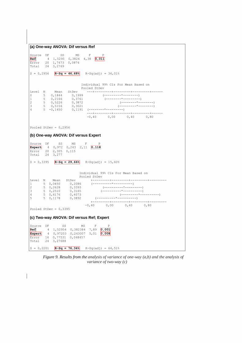
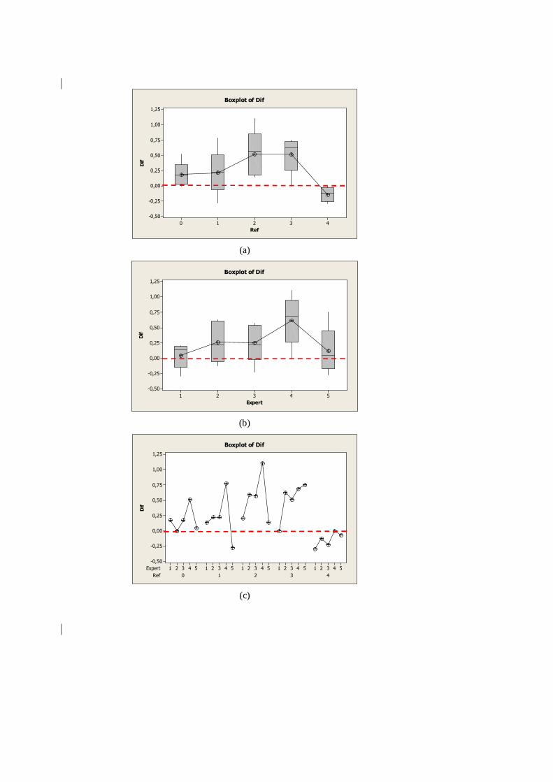
COMPARATIVE STATISTICAL ANALYSIS OF THE COLLECTED DATA In order to analyze if there are significant differences between the experts assessment and the reference values, an analysis of variance ANOVA (Johnson and Wichern 2002) of one and two factors has been carried out for the arithmetic means observed in the categorical variables "reference value" and "expert". The aim is to determine if the differences observed (Dif) are subject to a "reference value" effect and / or an "expert" effect. The results of the one and two factor ANOVA analysis for the referred variables, as well as the respective boxplots are shown in Figure 9 and Figure 10, respectively.
If it is decided at a significance level of 0.01 it can be seen that there is no "reference value" effect (p-value = 0.011 > 0.01), nor "expert" effect (p-value = 0.118 > 0.01). Similarly, the explanation percentages of the model are low (46.68% and 29.66%, respectively), in agreement with the existing overlaps on the one hand between the 99% confidence intervals for the respective means (Figure 9), and on the other hand, the overlaps between the associated boxplots (Figure 10a and Figure 10b). Thus, it may be concluded that the differences between the values of the experts with respect to the respective reference values are: 1) independent of the reference values and 2) independent of the experts.
However, it should be highlighted the existence of an effect of the interaction between the variable "reference value" and the variable "expert" (Figure 9c); interaction that
explains 76.34% of the variability with respect to the reference values or pattern. In other words, there is an individual sensitivity of the experts associated with the underlying level of probability of detachment. This sensitivity is evidenced in the observations in the reference value 2 of the expert T4 (Figure 10c).
Table 4. Statistical data of the assessment of the experts stratified with respect to the
reference values or pattern (T0)
Figure 8. Boxplot of the statistical data of the assessment of the experts stratified with respect to the reference values or pattern (T0)
However, because the total sample size is small (25 arithmetic means), we decided to apply a nonparametric approach, for the comparison of medians, in order to give more robustness to the analysis. For this it is used the Friedman Test (Coddington 1979), suitable for categorical and ordinal data. Figure 11 illustrates the results obtained from applying the Friedman Test to evaluate in terms of medians the differences between the values assigned by the experts with respect to the reference values or pattern. The results validate the non-significance of the differences (p = 0.05 > 0.01), and support the conclusions of independence cited in the previous paragraph. However, a higher contribution of the expert 4 can be appreciated again, although not significant, in the evaluation of the differences.
In conclusion, the previous analysis allows to validate: 1) the correct assignment of the reference values or pattern and 2) the representativeness of the average response values of the experts as evaluation of the detachment probability indicator.
Figure 9. Results from the analysis of variance of one-way (a,b) and the analysis of
variance of two-way (c)
Figure 10. Boxplots of the mean differences of the values assigned by the experts with respect to the reference values or pattern
Figure 11. Results from the Friedman Test
Binary identification of façade deteriorations
As mentioned, the objective of this research is to reduce the variability between inspectors in the assignment of values y, based on the symptomatology of the façade. In the present subsection the variables and values that collect the symptoms on the façade are described. The most common and representative deteriorations that a façade can have are the following:
· Humidity · Corrosion of reinforcements or metallic elements · Debonding, loose of materials · Cracks · Vegetation · Stains, efflorescence
· Loss of section, erosion The use of a binary assignment system with respect to these deteriorations is proposed, with the following criteria:
· 0 means the non-existence of the deterioration · 1 means the existence of the deterioration
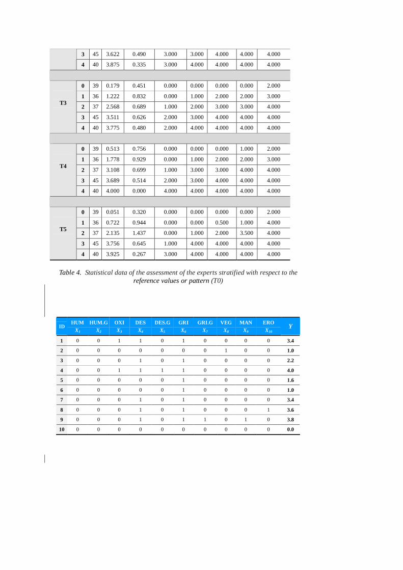
In a complementary way for those deteriorations more related to the probability of detachment, it has been considered convenient to also collect the degree of gravity of the deterioration. To this end, auxiliary variables have been defined binary for humidity, debonding and cracking dysfunctions. Table 5 shows, as an example, data for the first 10 images, where the columns represent: identification of each of the images (ID); humidity (HUM); severe humidity (HUM.G); oxidation (OXI); debonding (DES); serious debonding (DES.G); crack (GRI); severe crack (GRI.G); vegetation (VEG); stains (MAN); erosion (ERO); and the mean value of y assigned by the 5 experts (Y).
Table 5. Data of deteriorations and average assignments of experts for the first 10 images Regression model for the estimation of y In order to estimate the variable y from the deteriorations, the following multivariate linear regression model is proposed (Montgomery et al., 2012):
ij
jiji xy ebb å=
+×+=10
10 with ( )2,0~ se Ni , (7)
for i = 1,…, 197, where,
· yi = it is the variable to be explained, dependent or returning, in this case the variable associated with the probability of detachment measured on the individual (image) i-th, resulting from the average of the experts' assessments, with a normal distribution in each one of the reference values or pattern.
· 0b = intercept term
· jb = coefficient corresponding to the j-th deterioration, which measures the effect of this deterioration in the measure of the probability of detachment
· jix = explanatory variable, in this case the binary value corresponding to the j-th
deterioration measured on the individual (image) i-th
· ie = random error term of the regression model (independent and normally distributed)
With the statistical program Minitab® (Minitab 2017), the best multivariate linear
regression model has been estimated, which allows to adjust the available data and obtain inferences for the values of detachment probability, categorized in the objective variable y. For the selection of the model, the option Best Subsets has been used. Best Subsets is a decision strategy in regression analysis, based on the comparison of all possible models that can be created based on a given set of predictors. The independent variables or possible predictors in the final linear model are those presented in Table 5: HUM, HUM.G, OXI, DES, DES.G, GRI, GRI.G, VEG, MAN and ERO. Also preliminary regression models suggest the inclusion of the variable that collects the interaction between the existence of debondings and cracks. The sense of this variable is to collect the effect on the probability of detachment from the simultaneous presence of debondings and cracks. The interaction is denoted by DES*GRI (which takes the value 1 only when there is presence of both deteriorations). Figure 12 presents the statistical results of the estimation of the best models with a determined number of variables among the referred predictors, where:
· Vars: number of variables in the model
· R-square, ( )
( )å
å
=
=
-
-= n
ii
n
ii
yy
yyR
1
2
1
2
2ˆ
: proportion in percentage of variability in the data
explained by the model, where iy is the value estimated by the model for the i-th individual and y is the average of the data
· R-square (adjusted), ( ) ( )1111 22
+--
×--=kn
nRRadj : proportion in percentage of
variability in the data explained by the model penalized by the number of variables (k) in the model
· Cp de Mallows: measure of the bias in the estimation of the regression coefficients
· S, ( ) ( )å=
-×+-
=n
iii yy
knS
1
2ˆ1
1 : residual variance
· Explanatory variables in the study. The "X" sign denotes the inclusion in the model
Figure 12. Summary of statistics for the selection of the model and proposed model (in box)
For the selection of the initial model to be adjusted, the following criteria are considered:
a. Maximize 2
adjR , in order to obtain the maximum explicability of the model with the
least number of variables (simplicity in the model or principle of parsimony in statistics).
b. Minimize S in order to achieve homogeneity among the residuals.
c. Cp next to Vars + 1 given that Cp = Vars + 1 indicates absence of bias in the estimation of the regression values (Mallows 1973).
According to these criteria, as can be seen in Figure 12, the model that best fits the data, which it is called M1, is the one formed by the following eight indicators: HUM, DES, DES.G, GRI, GRI. G, MAN, ERO, DES*GRI. The estimation of coefficients of M1, as well as the variability of the estimators of the parameters is shown in Figure 13. As can be seen, although the M1 model has a high explanation of the variability (83.0%), there are two variables whose coefficient in the model is not significantly different from zero. These are the variables MAN and ERO (in Figure 13 delimited in red box, p-value > 0.05). In order to obtain a model with only significant variables, and with the same selection criteria, it is chosen in Figure 12 the following candidate that is the model, M2, formed by the six variables HUM, DES, DES.G, GRI, GRI.G and DES*GRI. The results of the estimation of the M2 model are presented in Figure 14. Figure 13. Estimations of the coefficients in the model M1, variability and significance of
the coefficients
Figure 14. Estimations of the coefficients in the model M2, variability and significance of
the coefficients
As can be seen in Figure 14, all variables of the M2 model are highly significant (p-value < 0.001). An analysis of the variance of the residuals also allows to conclude the goodness of the M2 model and, overall, its high significance. Finally, Figure 15 shows the validation of the model in terms of residuals analysis in order to illustrate the hypothesis of normality and independence. Therefore, the model based on the observed dysfunctions and that allows to reduce the variability between technicians is the following Equation. y = 0.268 + 0.409 HUM + 2.680 DES + 0.586 DES.G + 1.595 GRI + 0.658 GRI.G – 1.462 DES*GRI (8)
The model collects the presence and also gravity, of humidities, debondings and cracks. It is important to highlight the contribution of the presence of debondings (+2.680) and of cracks (+1.599), even more in the case of being severe (+0.586 and +0.658, respectively). Note, also, the compensating effect of the simultaneous presence of debondings and cracks (-1.462). Figure 15. Graphs of residuals (normality test, point cloud according to predicted values,
histogram, point cloud according to observation order) As an illustration of the fact that model M2 in Equation (8) gives a coherent answer, in constructive terms, to the range of values of the proposed scale, Table 6 shows the values estimated by the model for the different scenarios of observed deteriorations, and their respective qualitative values. By way of conclusion and procedure, the qualifications in essence collect the following configurations of symptoms:
· Very low: As it is reasonable, to obtain this qualification there should not be any deterioration.
· Low: There should be only humidities.
· Medium: There should be cracks, or the combination of these with humidities.
· High: There are several possible combinations shown in Table 6 in the light brown
colored section. As it is appreciated, only the presence of debondings or severe cracks is enough to obtain this qualification.
· Very high: There are also several possible combinations. In the dark pink colored section it can be seen that the severe debonding, or the debonding with severe crack characterize this qualification.
Table 6. Estimated values by the model for the different scenarios of observed deteriorations, ordered from the estimated values, y
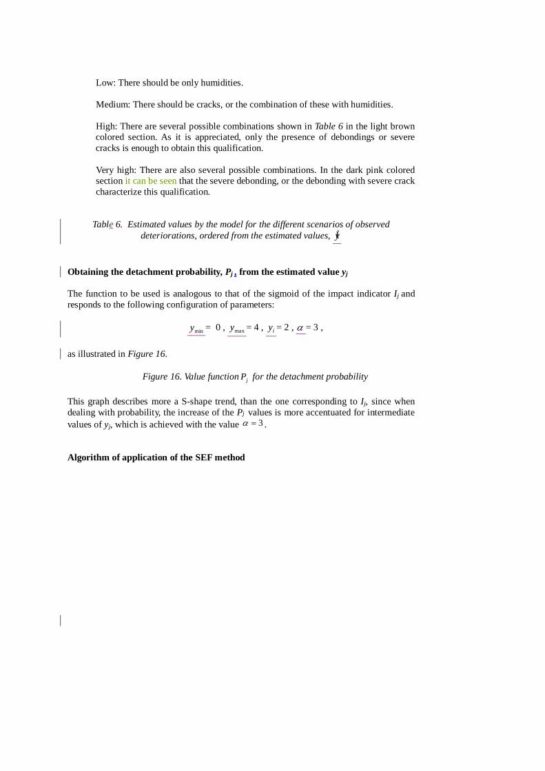
Obtaining the detachment probability, Pj , from the estimated value yj
The function to be used is analogous to that of the sigmoid of the impact indicator Ij and responds to the following configuration of parameters:
miny = 0 , maxy = 4 , iy = 2 , a = 3 ,
as illustrated in Figure 16.
Figure 16. Value function jP for the detachment probability
This graph describes more a S-shape trend, than the one corresponding to Ij, since when dealing with probability, the increase of the Pj values is more accentuated for intermediate values of yj, which is achieved with the value 3=a .
Algorithm of application of the SEF method
The methodology proposed in the previous sections can be summarized in the following algorithm, applied to each zone j of the façade delimited in the graphical part of the method:
Step 1: Identification of physical characteristics (see Table 1). Step 2: Calculation of xj, using the proposed Equation (3). Step 3: Calculation of Ij, using the sigmoid proposed in Figure 5. Step 4: Identification of the associated symptomatology. Step 5: Estimation of yj, using the Equation (8). Step 6: Calculation of Pj , using the sigmoid proposed in Figure 16. Step 7: Calculation of Gj , using the Equation (1).
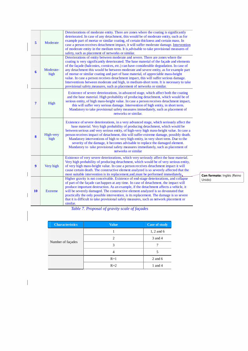
3. Introduction to intervention phase Although this paper focuses in assessing G values of severity of façades (diagnosis phase), and not in the derived decisions (intervention phase) from the diagnosis, it is considered suitable to explain some relations between diagnosis and derived interventions, in order to highlight the importance of the diagnosis phase. Thus Table 7 shows the general description of each G value (from G = 0 to G = 10). In this description are also included the suitable interventions for each G value.
Table 7. Proposal of gravity scale of façades
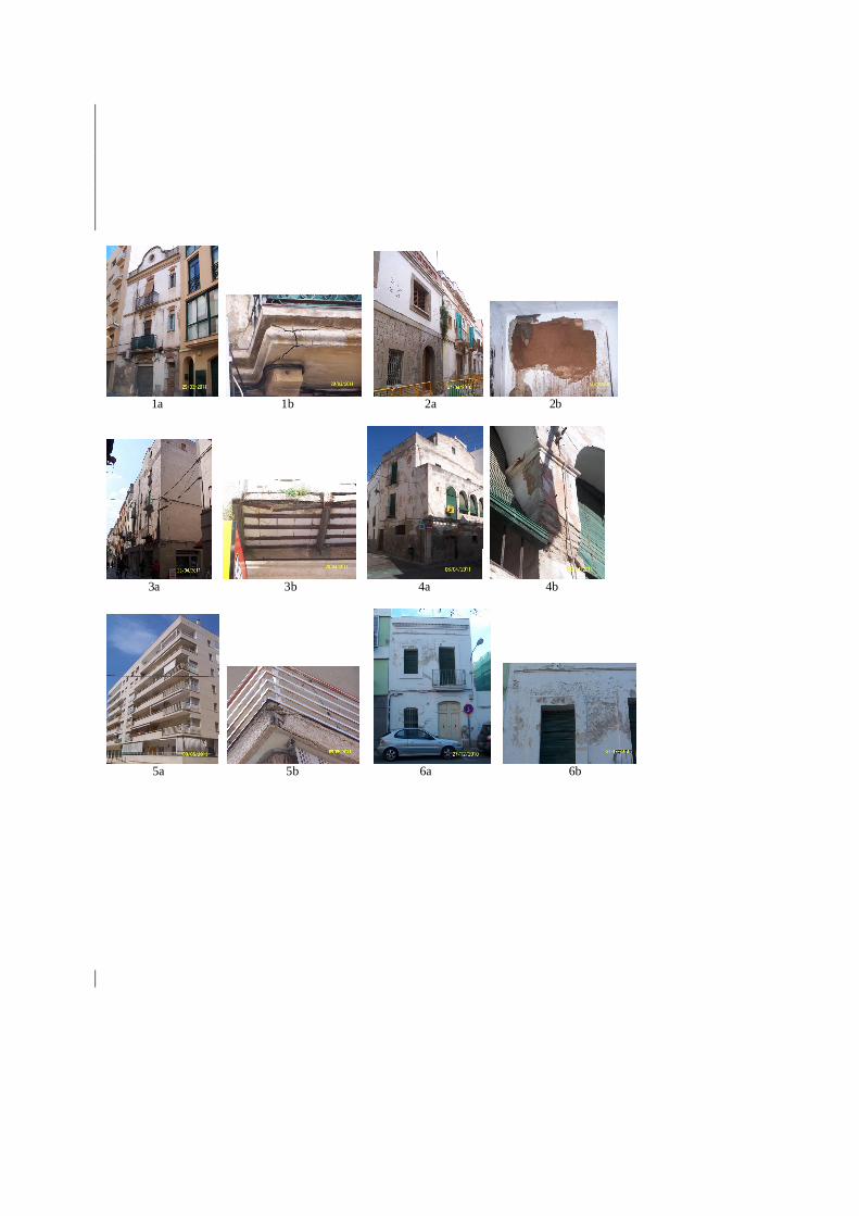
In Figure 17 is explained the general relation between G values and derived interventions. Hence the Figure represents that the entity of the intervention or therapeutic (represented in the line T) must be proportional (represented with the orange arrow) to the level of deterioration or G value (represented in the line G). Thus it must not be lower (represented with the red arrow) because then the intervention would be insufficient and it must not be higher (represented with the blue arrow) because then it would be oversized and in consequence the cost of the intervention would be higher than needed.
Figure 17. Relation between G value and therapeutic intervention value T
4. Practical application of SEF As a final part of the study, the practical application of the proposed methodology SEF to real cases of buildings is carried out. With the aim of incorporating a wide range of cases, both in construction types and amount of damages, the total number of buildings selected and inspected has been seven. In this way there are buildings between dividing walls with a
single main facade, others with two main facades, and isolated building with four main façades. The age range of the buildings in the sample varies from 30 years to more than two centuries. There are a variety of materials such as brick, rammed earth, stone, reinforced concrete, metal profiles, etc. There are several deteriorations, such as loss of section in the brick masonry, fractures in cantilevered stone, carbonation of concrete and corrosion of reinforcements, debonding of the coating, loss of section of the rammed earth, corrosion of metal profiles, etc. These cases can be seen in detail in (Ruiz 2014a).
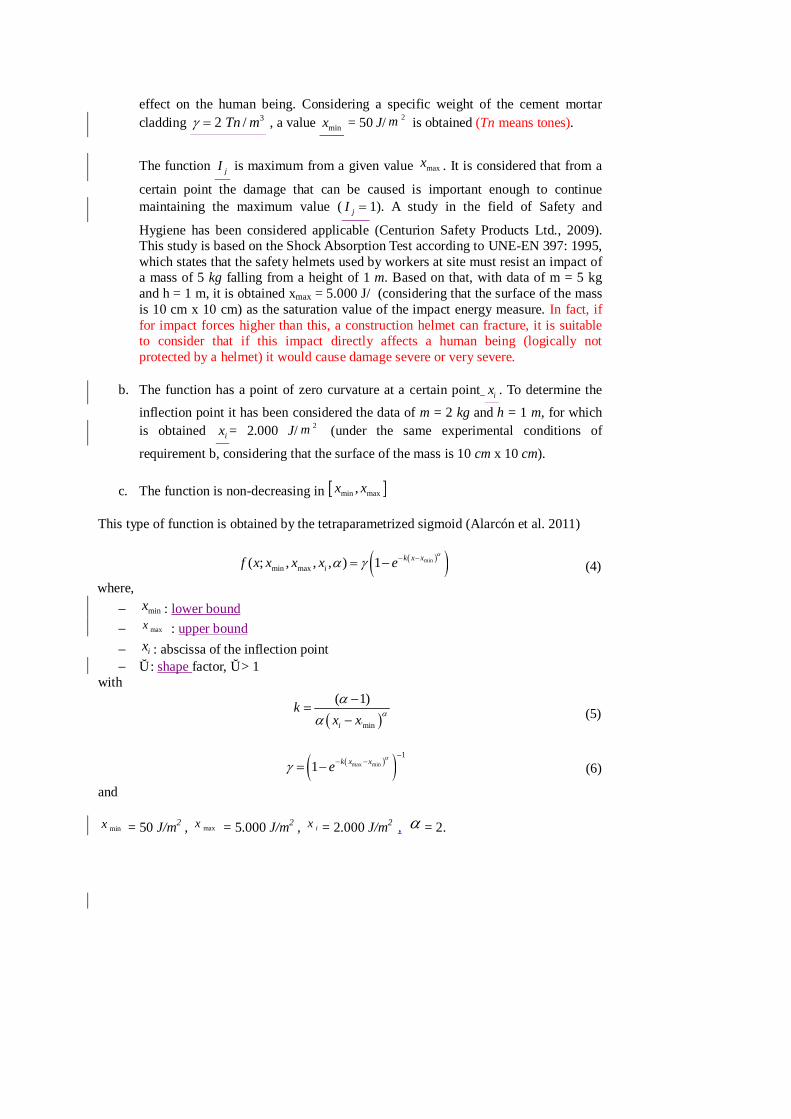
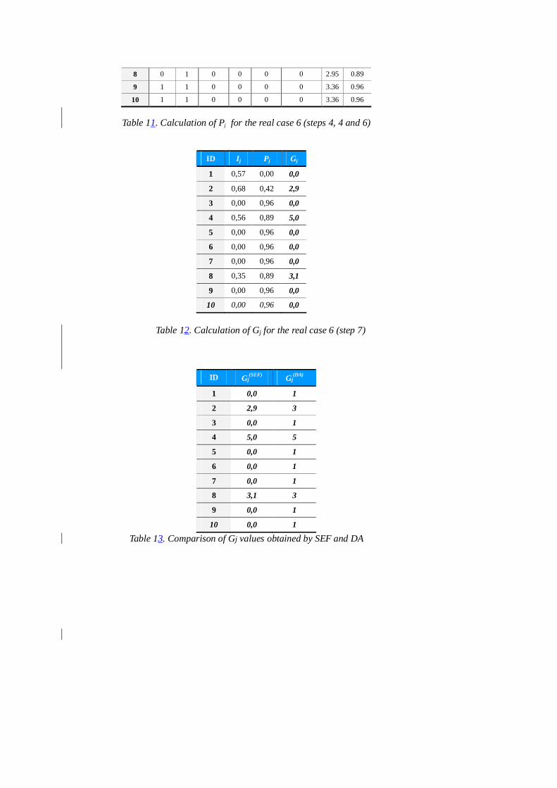
In order to illustrate the variety of cases of the selected case studies, in Figure 18 there are 14 images of these seven cases, with two images (a and b) of each case, the first one corresponds to a general view and the second one (b) a detailed view of a specific facade area. Similarly, a summary of the characteristics of the selected case studies is presented in Table 8. In it no rear façades are included, since the inspections have been made from the street. In the same way, as an example, one of the seven studied buildings is presented (corresponding to images 6a and 6b of Figure 18). Therefore, in Figure 19 and in Tables 9, 10, 11 and 12 are presented data of the deteriorated zones of the studied building and the obtained values of Ij , Pj and G
j for this zones, through using the SEF methodology.
Figure 18. Fourteen images of the seven studied cases
Table 8. Characteristics of the studied cases
Figure 19. Graphical representation of the façade of the real case 6, with delimitation of the deteriorated zones (step 1) (see Table 9 for description of type of deterioration)
Table 9. File of inspection of the real case 6 (step 2)
Table 10. Calculation of Ij for the real case 6 (step 3)
Table 11. Calculation of Pj for the real case 6 (steps 4, 4 and 6)
Table 12. Calculation of Gj for the real case 6 (step 7)
Once the Gj values of the different areas of the façades have been calculated using the SEF methodology proposed in this paper, SEF
jG the total gravity of the system façades ( )srwG of
each building can be calculated through the methodology proposed in (Ruiz 2014a), DAjG .
The results obtained by applying the SEF method to real cases are reasonable,
consistent with those that would result from the direct assignment method (DA). It is also interesting to mention that with respect to the values that would be obtained by applying the DA method, SEF homogenizes in some cases the values very close to both extremes, due to the characteristics of the proposed sigmoid value functions. For example, some direct assignments with value 1 (very low gravity) with SEF can result value 0 (perfect
condition), and similarly some direct assignments with value 9 (very high gravity) with SEF can result value 10 (extreme gravity; it is not conceivable greater gravity). The comparison of values of Gj of this studied building obtained through SEF and DA is presented in Table 13. It is observed the behavior discussed above with respect to extreme values. Thus, it is observed that for very low gravity values through DA (G = 1), a value of G = 0 is obtained through SEF. Out of the extreme values, the results compared between SEF and DA are the same or very similar. In the other six studied buildings the results indicate the same behavior that has been explained (Ruiz, 2014a).
Table 13. Comparison of Gj values obtained by SEF and DA 5. Conclusions The proposed assessment method of building façades and its practical application has derived in the following conclusions: The method presents two parts: graphical and numerical. In the first part, the façade and the zones of interest are defined. The zones of interest or analysis are obtained based on the observed damages, the type of material and the constructive elements (balconies, cornices, etc.). Starting from this graphical information, in the numerical part, the indicators necessary to assess the state of the façade regarding the risk of falling elements and their impact on people are computed according to the proposed mathematical expressions. The main indicators proposed are the impact energy of the falling element and the probability of detaching of this element from the façade. Using those parameters the uncertainty associated to the assessing methodology due to the inspector subjectivity is minimized as the proposed indicators are fully objective and measurable.
The equation allowing to calculate the impact energy takes into account the mass, the height and the surface of the falling element. The indicator probability of detaching is obtained based on a survey to five experts which were asked to quantify the probability of failure of several zones identified in 197 images of deteriorated façades. The application of the proposed method to seven real buildings has shown that the results obtained with the present method are in accordance to those obtained using the direct assignment method (DA). It is also observed that SEF homogenizes in some cases the values very close to both extremes, due to the characteristics of the proposed sigmoid value functions.
In summary, the method achieves the target goal to decrease the level of variability among technicians to determine the degree of gravity (Gj values) when applying the SEF methodology, compared to the DA method. The determination of the G value facilitates the intervention decision, since the entity of the intervention must be proportional to the level of deterioration or G value. The proposed method SEF can be extended to other types of building elements (structures, roofs,...) and also to other infrastructures. Acknowledgements This research has been partially supported by grants MTM2015-64465-C2-1-R (MINECO
/ FEDER) from the Ministerio de Economía y Competitividad (Spain) and 2017 SGR 622 from the Departament d’Economia i Coneixement de la Generalitat de Catalunya. Authors are grateful to the five experts that generously collaborated in the statistical essay as well to the members of the IEMAE (Institute of Statistics and Mathematics Applied to the Building Construction) of the Barcelona School of Building Construction, because of their valuable comments and suggestions in the development of the work.
References Alarcón, B., Aguado, A., Manga, R. and Josa, A., 2011. A Value Function for Assessing
Sustainability: Application to Industrial Buildings. Sustainability. 3(1), 35-50. doi:10.3390/su3010035.
BRIME, 1999. Review of current practice for assessment of structural condition and classification of defects. Deliverable D2. BRIME PL97-2220.
Centurion Safety Products Ltd., 2009. Head Protection and Accessories. Coddington, A., 1979. Friedman’s Contribution to Methodological Controversy. British
Review of Economic Issues, 2 (4), 1-13. Díaz, C., Cornadó, C., Santamaría, P., Rosell, J. R., Navarro, A., 2015. Actuación
preventiva de diagnóstico y control de movimientos en los edificios afectados por subsidencia en el barrio de la Estación de Sallent (Barcelona). (Preventive action of diagnosis and control of movements in the buildings affected by subsidence in the neighborhood of the Sallent Station (Barcelona)). Informes de la Construcción, 67(538): e089, doi: http://dx.doi.org/10.3989/ic.13.168. (in Spanish)
Elhakeem, A. and Hegazy, T., 2012. Building asset management with deficiency tracking and integrated life cycle optimisation. Structure and Infrastructure Engineering . 8 (8), 729-738.
Flourentzou, F., Brandt, E. , Wetzel, C., 2000. MEDIC - A method to predicting residual service life and refurbishment investment budgets. Energy and Buildings . 31 , 167-170.
Frangopol, D.M. 2011. Life-cycle performance, management and optimisation of structural systems under uncertainty: accomplishments and challenges. Structure and Infrastructure Engineering . 7(6), 389-413.
Gibert, V., 2016. Sistema predictivo multiescala de la degradación del frente urbano edificado. (Multiscale predictive system for the degradation of the built urban front). PhD Thesis. Barcelona School of Building Construction. Technical University of Catalonia-Barcelona-Tech. (in Spanish)
Herz, R., 1998. Exploring rehabilitation needs and strategies for drinking water distribution networks. Proceedings of the 1st IWSA/AISE Conference, Prague, Czech Republic.
Johnson, R.A. and Wichern, D.W. 2002. Applied Multivariate Statistical Analysis. Prentice Hall, New Jersey.
Kim, S. and Frangopol, D.M. 2017. Efficient multi-objective optimisation of probabilistic service life management. Structure and Infrastructure Engineering . 13 (1), 147-159.
Klein J.P. and Moeschberger M.L., 2003. Survival analysis: Techniques for censored and truncated data. Springer-Verlag.
Kobayashi, K. and Kaiko, K. 2017. Big data-based deterioration prediction models and infrastructure management: towards assetmetrics. Structure and Infrastructure Engineering . 13 (1), 84-93.
Kohler, N. and Yang, D., 2007. Long-term management of building stocks. Building Research and Information, 35(4), 351-362.
Li, J., Masia, M.J., Steward, M.J. 2017. Stochastic spatial modeling of material properties and structural strength of unreinforced masonry in two-way bending. Structure and Infrastructure Engineering . 13 (6), 683-695.
Mallows, C.L. 1973. Some Comments on CP. Technometrics 15 (4), 661-675. Mazzuchi, T.A. and René, J., 2012. A Bayesian expert judgement model to determine
lifetime distributions for maintenance optimisation. Structure and Infrastructure Engineering . 8 (4), 307-315.
Minitab Inc. 2017. Minitab.com. Retrieved 9 January 2018, from http://www.mionitab.com/en-us/
Miyamoto, A., Kawamura, K., Nakamura, H., 2000. Bridge management system and maintenance optimization for existing bridges. Computer-Aided Civil and Infrastructure Engineering, 15, 45-55.
Montgomery, D.C., Peck, E.A., Vining, G.G. 2012. Introduction to Linear Regression Analysis. 5th Edition. Wiley Series in Probability and Statistics. Wiley.
Neto, N. and de Brito, J., 2012. Validation of an inspection and diagnosis system for anomalies in natural stone cladding (NSC). Construction and Building Materials, 30: 224-236, doi:http://dx.doi.org/10.1016/j.conbuildmat.2011.12.032.
Pardo, F. and Aguado, A. 2017. Damage Diagnosis in Concrete Dams with Presented Expansive Damage Based on Medical Propaedeutics. American Society of Civil Engineers. 1-12. doi: 10.1061/(ASCE)CF.1943-5509.0001035.
Roche, J.M., 2008. Monitoring Inequality among Social Groups: A Methodology Combining Fuzzy Set Theory and Principal Component Analysis. Journal of Human Development and Capabilities (HDCA). New York, 9 (3), 427-452.
Rodrigues, M.F.S., Teixeira, J.M.C., Cardoso, J.C.P., 2011. Building envelope anomalies: A visual survey methodology. Construction and Building Materials, 25(6): 2741-2750, doi: http://dx.doi.org/10.1016/j.conbuildmat.2010.12.029.
Ruiz, F., 2014a. Escala de gravedad de daños en edificios: de la asignación directa a la constrastación estadística. (Severity scale of deterioration in buildings: from the direct assignment to statistical comparison). Doctoral Thesis. School of Civil Engineering. Technical University of Catalonia. Barcelona-Tech. http://hdl.handle.net/10803/285004. (in Spanish)
Ruiz, F., 2014b. La importància del manteniment i de les inspeccions periòdiques. Reflexions sobre un accident recent per despreniments de façana. (The importance of maintenance and periodic inspections. Reflections on a recent accident due to detachment of a façade). L’Informatiu. Association of Building Engineers of Barcelona. 341, 84-87. https://issuu.com/sia16/docs/inf341. (in Catalan)
Ruiz, F., 2013. Diagnosi de parets de tàpia. (Diagnosis of rammed earth walls). L’Informatiu. Association of Building Engineering of Barcelona. 335, 58-65. http://www.a16-01.com/pdfs/COL/2013/i335_58_65.pdf (in Catalan)
Ruiz, F., Aguado, A. Serrat C., Casas, J.R., 2019. Optimal metric for condition rating of existing buildings: is five the right number? Structure and Infrastructure Engineering.
doi: 10.1080/15732479.2018.1557702. Schiller, G., 2007. Urban infrastructure – challenges for resource efficiency in the building
stock. Building Research and Information, 35(4), 399-411. Serrat, C. and Gibert, V., 2011. Survival analysis methodology for service life prediction
and building maintenance. Proceeding of the 12th International Conference on Durability of Building materials and Components. Vol. II, Porto, Portugal, 599-606.
Silvestre, J.D., de Brito, J., 2011. Ceramic tiling in building façades: Inspection and pathological characterization using an expert system. Construction and Building Materials, 25(4): 1560-1571, doi: http://dx.doi.org/10.1016/j.conbuildmat.2010.09.039.
Sykora, M., Diamantidis, D., Holicky, M. Jung, K. 2017. Targer reliability for existing structures considering economic and social aspects. Structure and Infrastructure Engineering . 13 (1), 181-194.
Yang, D., 2006. International migration, remittances, and household investment: evidence from Philippine migrants exchange rate stocks. National Bureau of Economic Researh. Cambridge.
Figure 1. Outline of the methodology SEF (System of Evaluation of Façades)
Data collection
Graphical representation of the façade
Delimitation of deteriorated zones
Calculation of the impact energy indicator of detachment
Calculation of the probability indicator of
detachment
Calculation of the degree of gravity of zone j of the façade (Gj)
Numerical part
Graphical part
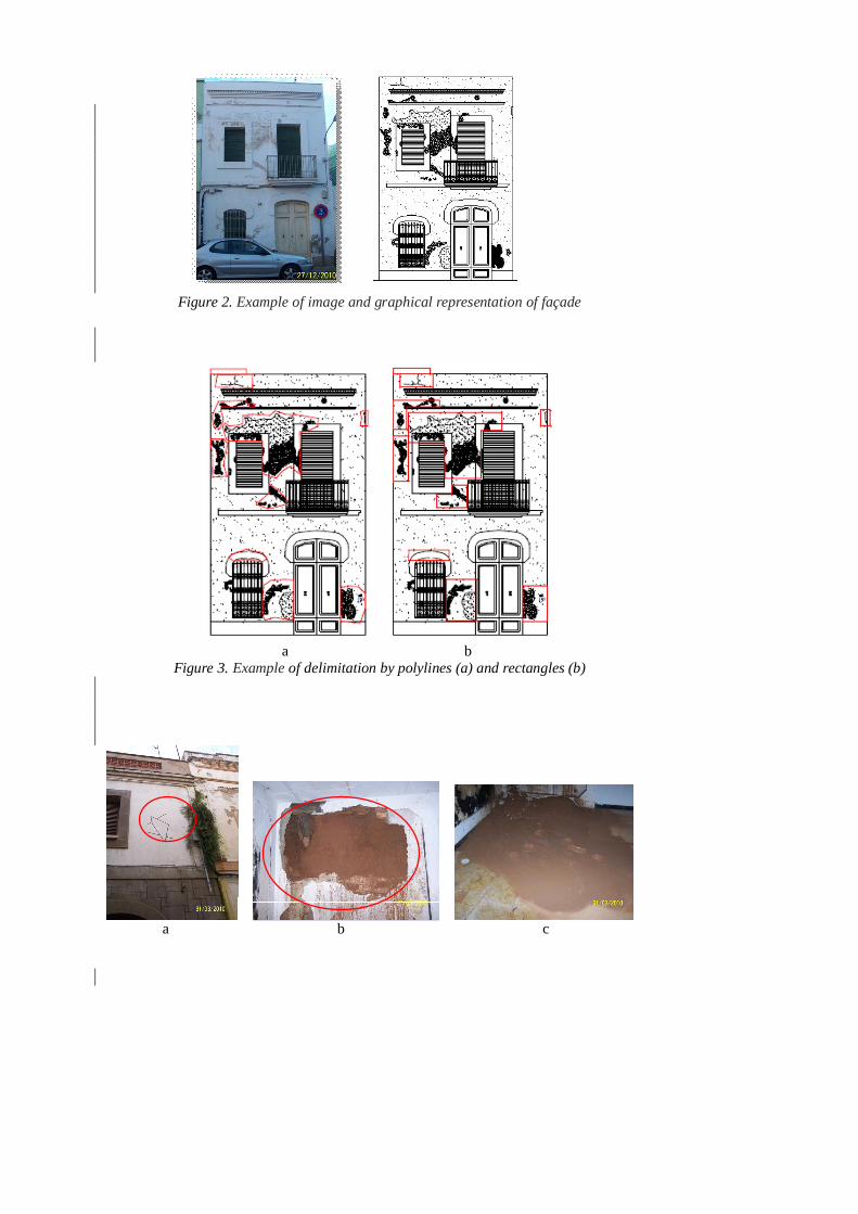
Figure 2. Example of image and graphical representation of façade
a b
Figure 3. Example of delimitation by polylines (a) and rectangles (b)
a b c
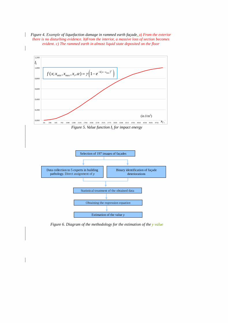
Figure 4. Example of liquefaction damage in rammed earth façade. a) From the exterior there is no disturbing evidence. b)From the interior, a massive loss of section becomes
evident. c) The rammed earth in almost liquid state deposited on the floor
0,000
0,200
0,400
0,600
0,800
1,000
1,200
50 298 545 793 1040 1288 1535 1783 2030 2278 2525 2773 3020 3268 3515 3763 4010 4258 4505 4753 5000 Figure 5. Value function Ij for impact energy
Figure 6. Diagram of the methodology for the estimation of the y value
Selection of 197 images of façades
Data collection to 5 experts in building pathology. Direct assignment of y
Binary identification of façade deteriorations
Statistical treatment of the obtained data
Obtaining the regression equation
Estimation of the value y
xj
Ij
(in J/m2)
( )( )minmin max( ; , , , ) 1 k x x
if x x x x ea
a g - -= -
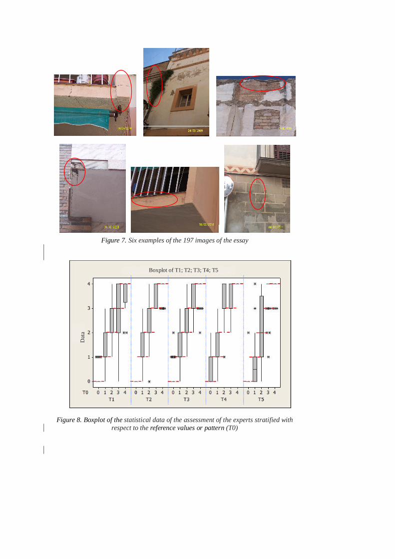
Figure 7. Six examples of the 197 images of the essay
Figure 8. Boxplot of the statistical data of the assessment of the experts stratified with respect to the reference values or pattern (T0)
Dat
a
Boxplot of T1; T2; T3; T4; T5
(a) One-way ANOVA: Dif versus Ref Source DF SS MS F P Ref 4 1,5295 0,3824 4,38 0,011 Error 20 1,7473 0,0874 Total 24 3,2769 S = 0,2956 R-Sq = 46,68% R-Sq(adj) = 36,01% Individual 99% CIs For Mean Based on Pooled StDev Level N Mean StDev ---+---------+---------+---------+------ 0 5 0,1844 0,1999 (---------*--------) 1 5 0,2166 0,3761 (--------*---------) 2 5 0,5226 0,3872 (--------*--------) 3 5 0,5156 0,3021 (---------*--------) 4 5 -0,1450 0,1191 (--------*---------) ---+---------+---------+---------+------ -0,40 0,00 0,40 0,80 Pooled StDev = 0,2956 (b) One-way ANOVA: Dif versus Expert Source DF SS MS F P Expert 4 0,972 0,243 2,11 0,118 Error 20 2,305 0,115 Total 24 3,277 S = 0,3395 R-Sq = 29,66% R-Sq(adj) = 15,60% Individual 99% CIs For Mean Based on Pooled StDev Level N Mean StDev +---------+---------+---------+--------- 1 5 0,0450 0,2086 (----------*----------) 2 5 0,2628 0,3393 (----------*---------) 3 5 0,2510 0,3165 (----------*----------) 4 5 0,6176 0,4073 (---------*----------) 5 5 0,1178 0,3892 (----------*----------) +---------+---------+---------+--------- -0,40 0,00 0,40 0,80 Pooled StDev = 0,3395 (c) Two-way ANOVA: Dif versus Ref; Expert Source DF SS MS F P Ref 4 1,52954 0,382384 7,89 0,001 Expert 4 0,97203 0,243007 5,01 0,008 Error 16 0,77531 0,048457 Total 24 3,27688 S = 0,2201 R-Sq = 76,34% R-Sq(adj) = 64,51%
Figure 9. Results from the analysis of variance of one-way (a,b) and the analysis of
variance of two-way (c)
43210
1,25
1,00
0,75
0,50
0,25
0,00
-0,25
-0,50
Ref
Dif
Boxplot of Dif
(a)
54321
1,25
1,00
0,75
0,50
0,25
0,00
-0,25
-0,50
Expert
Dif
Boxplot of Dif
(b)
RefExpert
432105432154321543215432154321
1,25
1,00
0,75
0,50
0,25
0,00
-0,25
-0,50
Dif
Boxplot of Dif
(c)
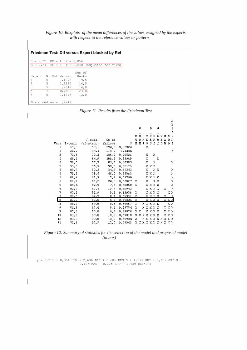
Figure 10. Boxplots of the mean differences of the values assigned by the experts with respect to the reference values or pattern
Friedman Test: Dif versus Expert blocked by Ref S = 9,32 DF = 4 P = 0,054 S = 9,51 DF = 4 P = 0,050 (adjusted for ties) Sum of Expert N Est Median Ranks 1 5 0,1292 9,5 2 5 0,2220 14,5 3 5 0,2642 14,0 4 5 0,6838 24,0 5 5 0,1718 13,0 Grand median = 0,2942
Figure 11. Results from the Friedman Test
Figure 12. Summary of statistics for the selection of the model and proposed model (in box)
y = 0,211 + 0,351 HUM + 2,636 DES + 0,605 DES.G + 1,599 GRI + 0,652 GRI.G +
0,125 MAN + 0,225 ERO - 1,439 DES*GRI
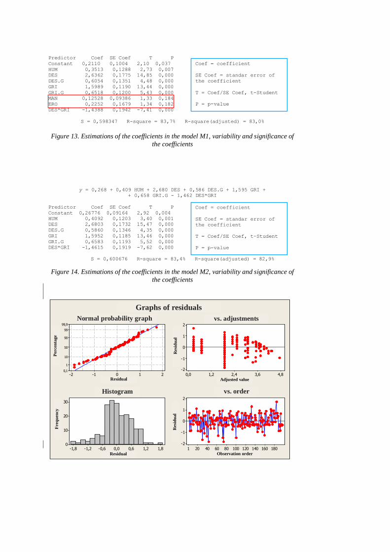
Predictor Coef SE Coef T P Constant 0,2110 0,1004 2,10 0,037 HUM 0,3513 0,1288 2,73 0,007 DES 2,6362 0,1775 14,85 0,000 DES.G 0,6054 0,1351 4,48 0,000 GRI 1,5989 0,1190 13,44 0,000 GRI.G 0,6518 0,1200 5,43 0,000 MAN 0,12528 0,09386 1,33 0,184 ERO 0,2252 0,1679 1,34 0,182 DES*GRI -1,4388 0,1942 -7,41 0,000
S = 0,598347 R-square = 83,7% R-square(adjusted) = 83,0%
Figure 13. Estimations of the coefficients in the model M1, variability and significance of
the coefficients
y = 0,268 + 0,409 HUM + 2,680 DES + 0,586 DES.G + 1,595 GRI + + 0,658 GRI.G - 1,462 DES*GRI
Predictor Coef SE Coef T P Constant 0,26776 0,09164 2,92 0,004 HUM 0,4092 0,1203 3,40 0,001 DES 2,6803 0,1732 15,47 0,000 DES.G 0,5860 0,1346 4,35 0,000 GRI 1,5952 0,1185 13,46 0,000 GRI.G 0,6583 0,1193 5,52 0,000 DES*GRI -1,4615 0,1919 -7,62 0,000
S = 0,600676 R-square = 83,4% R-square(adjusted) = 82,9%
Figure 14. Estimations of the coefficients in the model M2, variability and significance of
the coefficients
Coef = coefficient SE Coef = standar error of the coefficient T = Coef/SE Coef, t-Student P = p-value
Coef = coefficient SE Coef = standar error of the coefficient T = Coef/SE Coef, t-Student P = p-value
210-1-2
99,999
90
50
10
10,1
Residuo
Porc
enta
je
4,83,62,41,20,0
2
1
0
-1
-2
Valor ajustado
Resi
duo
1,81,20,60,0-0,6-1,2-1,8
30
20
10
0
Residuo
Frec
uenc
ia
180160140120100806040201
2
1
0
-1
-2
Orden de observación
Resi
duo
Gráfica de probabilidad normal vs. ajustes
Histograma vs. orden
Gráficas de residuos para VAL_Pvs. adjustments
Perc
enta
ge
Fr
eque
ncy
Graphs of residuals
Res
idua
l
Res
idua
l
Residual
Residual
Histogram
Adjusted value
Observation order
vs. order
Normal probability graph
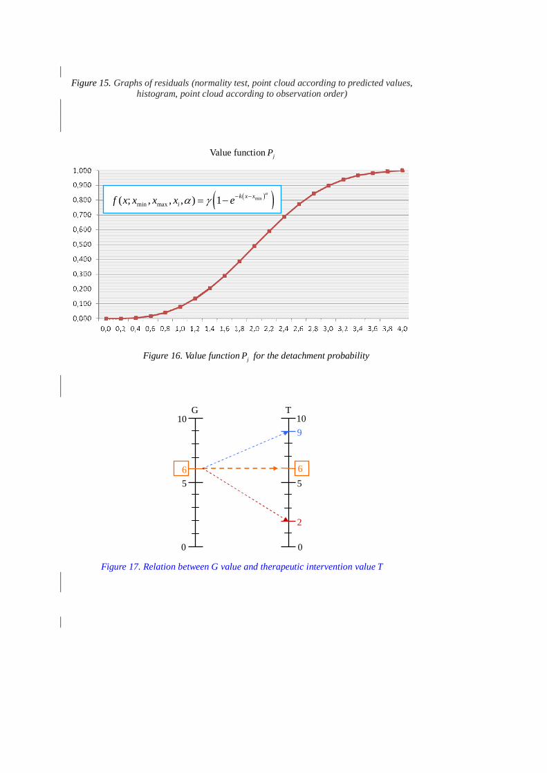
Figure 15. Graphs of residuals (normality test, point cloud according to predicted values,
histogram, point cloud according to observation order)
Figure 16. Value function jP for the detachment probability
Figure 17. Relation between G value and therapeutic intervention value T
G T
0 0
5 5
10 10
6 6
9
2
( )( )minmin max( ; , , , ) 1 k x x
if x x x x ea
a g - -= -
Value function jP
1a 1b 2a 2b
3a 3b 4a 4b
5a 5b 6a 6b
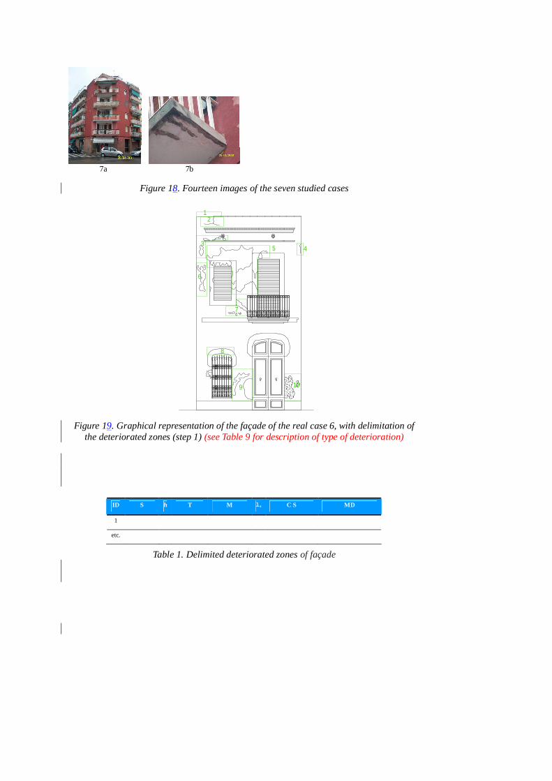
7a 7b
Figure 18. Fourteen images of the seven studied cases
Figure 19. Graphical representation of the façade of the real case 6, with delimitation of the deteriorated zones (step 1) (see Table 9 for description of type of deterioration)
ID S h T M ls C S MD 1
etc.
Table 1. Delimited deteriorated zones of façade
4
12
35
6
8
9 10
7
experts’ assessment ID T0 T1 T2 T3 T4 T5
mean ym1 (T1 - T5)
mean ym2 (T0 - T5)
1 3 3 3 3 4 4 3.4 3.3 2 1 1 1 0 2 1 1.0 1.0 3 2 2 3 2 2 2 2.2 2.2 4 4 4 4 4 4 4 4.0 4.0 5 1 2 3 0 0 3 1.6 1.5 6 1 1 2 1 1 0 1.0 1.0 7 3 3 4 4 3 3 3.4 3.3 8 3 4 4 3 4 3 3.6 3.5 9 3 4 4 4 4 3 3.8 3.7 10 0 0 0 0 0 0 0.0 0.0
Table 2. Assessment of the experts for the first 10 images of façades
Expert N Mean Std. Dev. Minimum Q1 Median Q3 Maximum T0 197 2.056 1.422 0.000 1.000 2.000 3.000 4.000 T1 197 2.112 1.491 0.000 1.000 2.000 4.000 4.000 T2 197 2.325 1.599 0.000 1.000 3.000 4.000 4.000 T3 197 2.310 1.512 0.000 1.000 3.000 4.000 4.000 T4 197 2.665 1.457 0.000 2.000 3.000 4.000 4.000 T5 197 2.198 1.775 0.000 0.000 3.000 4.000 4.000
Table 3. Statistical data of the assessment of the experts
Expert T0 N Mean Std. Dev. Minimum Q1 Median Q3 Maximum 0 39 0.179 0.389 0.000 0.000 0.000 0.000 1.000 1 36 1.139 0.723 0.000 1.000 1.000 2.000 3.000 2 37 2.297 0.968 1.000 2.000 2.000 3.000 4.000 3 45 3.000 1.044 0.000 2.000 3.000 4.000 4.000
T1
4 40 3.700 0.564 2.000 3.250 4.000 4.000 4.000
0 39 0.000 0.000 0.000 0.000 0.000 0.000 0.000 1 36 1.222 0.898 0.000 1.000 1.000 2.000 3.000
T2 2 37 2.595 0.896 0.000 2.000 3.000 3.000 4.000
3 45 3.622 0.490 3.000 3.000 4.000 4.000 4.000 4 40 3.875 0.335 3.000 4.000 4.000 4.000 4.000
0 39 0.179 0.451 0.000 0.000 0.000 0.000 2.000 1 36 1.222 0.832 0.000 1.000 2.000 2.000 3.000 2 37 2.568 0.689 1.000 2.000 3.000 3.000 4.000 3 45 3.511 0.626 2.000 3.000 4.000 4.000 4.000
T3
4 40 3.775 0.480 2.000 4.000 4.000 4.000 4.000
0 39 0.513 0.756 0.000 0.000 0.000 1.000 2.000 1 36 1.778 0.929 0.000 1.000 2.000 2.000 3.000 2 37 3.108 0.699 1.000 3.000 3.000 4.000 4.000 3 45 3.689 0.514 2.000 3.000 4.000 4.000 4.000
T4
4 40 4.000 0.000 4.000 4.000 4.000 4.000 4.000
0 39 0.051 0.320 0.000 0.000 0.000 0.000 2.000 1 36 0.722 0.944 0.000 0.000 0.500 1.000 4.000 2 37 2.135 1.437 0.000 1.000 2.000 3.500 4.000 3 45 3.756 0.645 1.000 4.000 4.000 4.000 4.000
T5
4 40 3.925 0.267 3.000 4.000 4.000 4.000 4.000
Table 4. Statistical data of the assessment of the experts stratified with respect to the reference values or pattern (T0)
ID HUM X1
HUM.G X2
OXI X3
DES X4
DES.G X5
GRI X6
GRI.G X7
VEG X8
MAN X9
ERO X10 Y
1 0 0 1 1 0 1 0 0 0 0 3.4 2 0 0 0 0 0 0 0 1 0 0 1.0 3 0 0 0 1 0 1 0 0 0 0 2.2 4 0 0 1 1 1 1 0 0 0 0 4.0 5 0 0 0 0 0 1 0 0 0 0 1.6 6 0 0 0 0 0 1 0 0 0 0 1.0 7 0 0 0 1 0 1 0 0 0 0 3.4 8 0 0 0 1 0 1 0 0 0 1 3.6 9 0 0 0 1 0 1 1 0 1 0 3.8 10 0 0 0 0 0 0 0 0 0 0 0.0
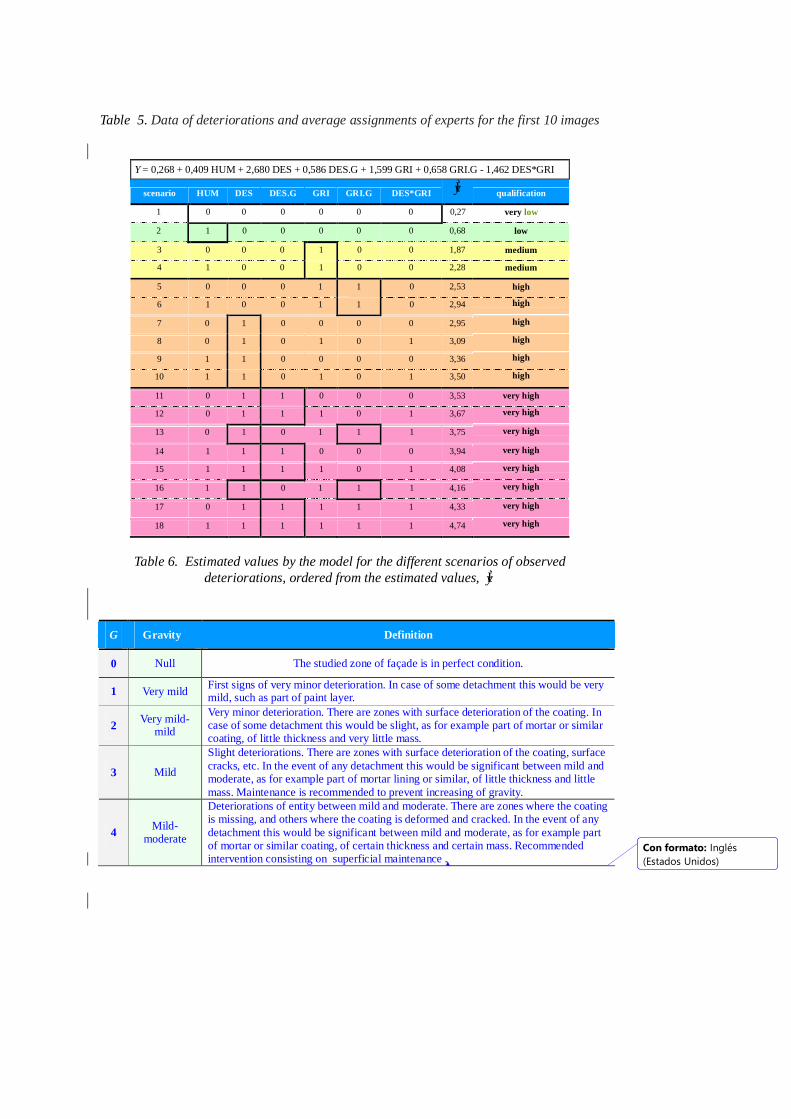
Table 5. Data of deteriorations and average assignments of experts for the first 10 images
Y = 0,268 + 0,409 HUM + 2,680 DES + 0,586 DES.G + 1,599 GRI + 0,658 GRI.G - 1,462 DES*GRI
scenario HUM DES DES.G GRI GRI.G DES*GRI y qualification 1 0 0 0 0 0 0 0,27 very low 2 1 0 0 0 0 0 0,68 low 3 0 0 0 1 0 0 1,87 medium 4 1 0 0 1 0 0 2,28 medium 5 0 0 0 1 1 0 2,53 high 6 1 0 0 1 1 0 2,94 high 7 0 1 0 0 0 0 2,95 high 8 0 1 0 1 0 1 3,09 high 9 1 1 0 0 0 0 3,36 high 10 1 1 0 1 0 1 3,50 high 11 0 1 1 0 0 0 3,53 very high 12 0 1 1 1 0 1 3,67 very high 13 0 1 0 1 1 1 3,75 very high 14 1 1 1 0 0 0 3,94 very high 15 1 1 1 1 0 1 4,08 very high 16 1 1 0 1 1 1 4,16 very high 17 0 1 1 1 1 1 4,33 very high 18 1 1 1 1 1 1 4,74 very high
Table 6. Estimated values by the model for the different scenarios of observed
deteriorations, ordered from the estimated values, y
G Gravity Definition
0 Null The studied zone of façade is in perfect condition.
1 Very mild First signs of very minor deterioration. In case of some detachment this would be very mild, such as part of paint layer.
2 Very mild-mild
Very minor deterioration. There are zones with surface deterioration of the coating. In case of some detachment this would be slight, as for example part of mortar or similar coating, of little thickness and very little mass.
3 Mild Slight deteriorations. There are zones with surface deterioration of the coating, surface cracks, etc. In the event of any detachment this would be significant between mild and moderate, as for example part of mortar lining or similar, of little thickness and little mass. Maintenance is recommended to prevent increasing of gravity.
4 Mild-moderate
Deteriorations of entity between mild and moderate. There are zones where the coating is missing, and others where the coating is deformed and cracked. In the event of any detachment this would be significant between mild and moderate, as for example part of mortar or similar coating, of certain thickness and certain mass. Recommended intervention consisting on superficial maintenance .
Con formato: Inglés(Estados Unidos)
5 Moderate
Deteriorations of moderate entity. There are zones where the coating is significantly deteriorated. In case of any detachment, this would be of moderate entity, such as for example part of mortar or similar coating, of certain thickness and certain mass. In case a person receives detachment impact, it will suffer moderate damage. Intervention of moderate entity in the medium term. It is advisable to take provisional measures of safety, such as placement of networks or similar.
6 Moderate-high
Deteriorations of entity between moderate and severe. There are zones where the coating is very significantly deteriorated. The base material of the façade and elements of the façade (balconies, cornices, etc.) can have considerable degradation. In case of any detachment this would be between moderate and severe entity, as for example part of mortar or similar coating and part of base material, of appreciable mass-height value. In case a person receives detachment impact, this will suffer serious damage. Interventions between moderate and high, in medium-short term. It is necessary to take provisional safety measures, such as placement of networks or similar.
7 High
Existence of severe deteriorations, in advanced stage, which affect both the coating and the base material. High probability of producing detachment, which would be of
serious entity, of high mass-height value. In case a person receives detachment impact, this will suffer very serious damage. Intervention of high entity, in short term.
Mandatory to take provisional safety measures immediately, such as placement of networks or similar.
8 High-very high
Existence of severe deteriorations, in a very advanced stage, which seriously affect the base material. Very high probability of producing detachment, which would be
between serious and very serious entity, of high-very high mass-height value. In case a person receives impact of detachment, this will suffer extreme damage, possibly death.
Mandatory interventions of high to very high entity, in very short term. Due to the severity of the damage, it becomes advisable to replace the damaged element.
Mandatory to take provisional safety measures immediately, such as placement of networks or similar
9 Very high
Existence of very severe deteriorations, which very seriously affect the base material. Very high probability of producing detachment, which would be of very serious entity, of very high mass-height value. In case a person receives detachment impact it will cause certain death. The constructive element analyzed is so severely affected that the most suitable intervention is its replacement and must be performed immediately.
10 Extreme
Higher gravity is not conceivable. Existence of end-stage deteriorations, and collapse of part of the façade can happen at any time. In case of detachment, the impact will produce important destruction. As an example, if the detachment affects a vehicle, it will be severely damaged. The constructive element analyzed is so devastated that practically the only possible intervention is its replacement. The damage is so severe that it is difficult to take provisional safety measures, such as network placement or similar.
Table 7. Proposal of gravity scale of façades
Characteristics Value Case of study 1 1, 2 and 6 2 3 and 4 3 7
Number of façades
4 5 R+1 2 and 6
R+2 1 and 4
Con formato: Inglés (ReinoUnido)
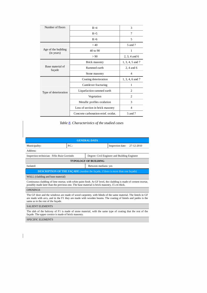
R+4 3 R+5 7
Number of floors
R+6 5 < 40 5 and 7
40 to 90 1
Age of the building (in years)
> 90 2, 3, 4 and 6 Brick masonry 1, 3, 4, 5 and 7 Rammed earth 2, 4 and 6
Base material of
façade Stone masonry 4
Coating deterioration 1, 3, 4, 6 and 7 Cantilever fracturing 1
Liquefaction rammed earth 2 Vegetation 2
Metallic profiles oxidation 3 Loss of section in brick masonry 4
Type of deterioration
Concrete carbonation-reinf. oxidat. 5 and 7
Table 8. Characteristics of the studied cases
GENERAL DATA
Municipality: P.C.: Inspection date: 27-12-2010 Address: Inspection technician: Félix Ruiz Gorrindo Degree: Civil Engineer and Building Engineer
TYPOLOGY OF BUILDING Isolated: Between medians: yes
DESCRIPTION OF THE FAÇADE (number the façade, if there is more than one façade) WALL (cladding and base material) Continuous cladding of lime mortar, with white paint finsh. At GF level, the cladding is made of cement mortar, possibly made later than the previous one. The base material is brick masonry, 15 cm thick. OPENINGS The GF door and the windows are made of wood carpentry, with blinds of the same material. The lintels in GF are made with arcs, and in the F1 they are made with wooden beams. The coating of lintels and jambs is the same as in the rest of the façade. SALIENT ELEMENTS The slab of the balcony of F1 is made of stone material, with the same type of coating that the rest of the façade. The upper cornice is made of brick masonry. SPECIFIC ELEMENTS
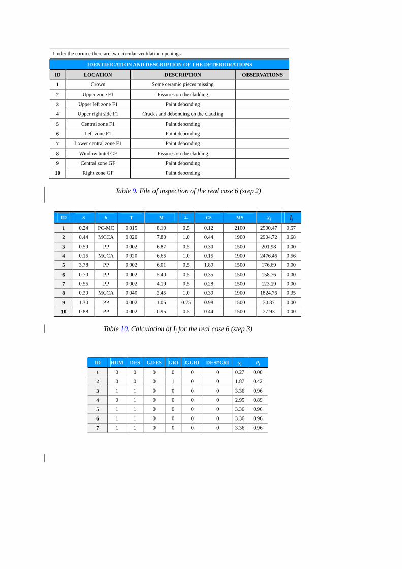
Under the cornice there are two circular ventilation openings. IDENTIFICATION AND DESCRIPTION OF THE DETERIORATIONS
ID LOCATION DESCRIPTION OBSERVATIONS 1 Crown Some ceramic pieces missing
2 Upper zone F1 Fissures on the cladding
3 Upper left zone F1 Paint debonding
4 Upper right side F1 Cracks and debonding on the cladding
5 Central zone F1 Paint debonding
6 Left zone F1 Paint debonding
7 Lower central zone F1 Paint debonding
8 Window lintel GF Fissures on the cladding
9 Central zone GF Paint debonding
10 Right zone GF Paint debonding
Table 9. File of inspection of the real case 6 (step 2)
ID S h T M ls CS MS xj Ij
1 0.24 PC-MC 0.015 8.10 0.5 0.12 2100 2500.47 0,57 2 0.44 MCCA 0.020 7.80 1.0 0.44 1900 2904.72 0.68 3 0.59 PP 0.002 6.87 0.5 0.30 1500 201.98 0.00 4 0.15 MCCA 0.020 6.65 1.0 0.15 1900 2476.46 0.56 5 3.78 PP 0.002 6.01 0.5 1.89 1500 176.69 0.00 6 0.70 PP 0.002 5.40 0.5 0.35 1500 158.76 0.00 7 0.55 PP 0.002 4.19 0.5 0.28 1500 123.19 0.00 8 0.39 MCCA 0.040 2.45 1.0 0.39 1900 1824.76 0.35 9 1.30 PP 0.002 1.05 0.75 0.98 1500 30.87 0.00 10 0.88 PP 0.002 0.95 0.5 0.44 1500 27.93 0.00
Table 10. Calculation of Ij for the real case 6 (step 3)
ID HUM DES G.DES GRI G.GRI DES*GRI yj Pj 1 0 0 0 0 0 0 0.27 0.00 2 0 0 0 1 0 0 1.87 0.42 3 1 1 0 0 0 0 3.36 0.96 4 0 1 0 0 0 0 2.95 0.89 5 1 1 0 0 0 0 3.36 0.96 6 1 1 0 0 0 0 3.36 0.96 7 1 1 0 0 0 0 3.36 0.96
8 0 1 0 0 0 0 2.95 0.89 9 1 1 0 0 0 0 3.36 0.96 10 1 1 0 0 0 0 3.36 0.96
Table 11. Calculation of Pj for the real case 6 (steps 4, 4 and 6)
ID Ij
Pj Gj
1 0,57 0,00 0,0
2 0,68 0,42 2,9
3 0,00 0,96 0,0
4 0,56 0,89 5,0
5 0,00 0,96 0,0
6 0,00 0,96 0,0
7 0,00 0,96 0,0
8 0,35 0,89 3,1
9 0,00 0,96 0,0
10 0,00 0,96 0,0
Table 12. Calculation of Gj
for the real case 6 (step 7)
ID Gj(SEF) Gj
(DA)
1 0,0 1
2 2,9 3
3 0,0 1
4 5,0 5
5 0,0 1
6 0,0 1
7 0,0 1
8 3,1 3
9 0,0 1
10 0,0 1
Table 13. Comparison of Gj values obtained by SEF and DA