research on real-time simulation system of ship motion

Send Orders for Reprints to [email protected]

820 The Open Mechanical Engineering Journal, 2014, 8, 820-827

1874-155X/14 2014 Bentham Open

Open Access Research on Real-Time Simulation System of Ship Motion Based on Simulink Yingfei Zan1, Duanfeng Han*,1, Lihao Yuan1, Minghao Liu1 and Zhaohui Wu2

1College of Shipbuilding Engineering, Harbin Engineering University, Harbin, 150001, China 2Offshore Oil Engineering Co., Ltd., Tianjin, 300451, China

Abstract: This paper puts forward a development method of ship motion simulation system that can conduct UDP communication in real time. This system is based on Simulink in order to meet the need of modular and fast ship motion simulation systems. First, the mathematics models of ship motion are set up based on the modular ideology, which includes thruster model and models of wind, wave and current. Then, real time simulation module using S-fun function is developed, and built into executable program. This could realize real time communication between ship motion simulation system and visual simulation system and induce real time communication between ship motion system and ship simulation control system. In this way, it can save time and cost when developing the simulation system. This method has been used successfully in the development of real time simulation system of some engineering ship.

Keywords: Real time simulation, Ship motion, Simulink, UDP communication.

1. INTRODUCTION

Real-time ship motion simulation system based on ship motion kinematic mathematical model utilizes computer simulation and human-computer interaction technology to acquire real-time interactive simulation of process of sailing and operation. The system possesses the ability of testing performance of ship motion, training ship operators and obtaining prediction and assessment of on-sea operation schemes, shortening the periods and costs of real-ship training and reducing the possibility of risky on-sea operation and damaged marine equipment, while effectively securing the safety of workers and equipment. However, adding UDP protocol module and real-time control mode into C mode transferred from Simulink model can attain executable program, greatly increasing the amount of work in post-processing and program changing [1]. In this paper, modular ship motion mathematical model is established including propeller model and wind, wave and current environmental models. UDP-based protocol is utilized to communicate directly with other systems and S-fun to develop real-time simulation module [2-4]. Finally, Simulink directly compiles an executable file to achieve a smooth transition from Simulink to real-time communication with other systems without post-processing and a perfect link between design phase and implementation phase is obtained.

2. SHIP MOTION MODEL

2.1. Establishment and Transformation of Coordinate

In order to describe ship motion at sea, two right-hand cartesian coordinates are needed: North-East-Down *Address correspondence to this author at the College of Ship Building Engineering, Harbin Engineering University, Harbin, 150001, China; Tel: +86-451-82519910; Fax: +86-451-82518443; E-mail: [email protected]

coordinate frame O0 ! x0y0z0 , which is an inertial frame for describing movement of ship; the other one is body-fixed kinematic frame G ! xyz , which is fixed to the ship with its origin at the center of gravity. These two frames are elaborated below[5]:

2.1.1. North-East-Down (NED) Coordinate System

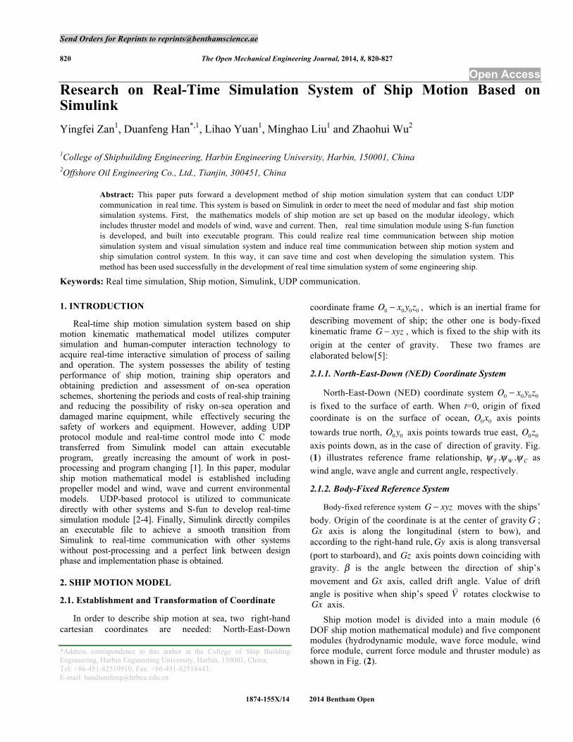
North-East-Down (NED) coordinate system O0 ! x0y0z0 is fixed to the surface of earth. When t=0, origin of fixed coordinate is on the surface of ocean, O0x0 axis points towards true north, O0y0 axis points towards true east, O0z0 axis points down, as in the case of direction of gravity. Fig. (1) illustrates reference frame relationship, ! T ,!W ,! C as wind angle, wave angle and current angle, respectively.

2.1.2. Body-Fixed Reference System

Body-fixed reference system G ! xyz moves with the ships’ body. Origin of the coordinate is at the center of gravityG ; Gx axis is along the longitudinal (stern to bow), and according to the right-hand rule,Gy axis is along transversal (port to starboard), and Gz axis points down coinciding with gravity. ! is the angle between the direction of ship’s movement and Gx axis, called drift angle. Value of drift angle is positive when ship’s speed

!V rotates clockwise to

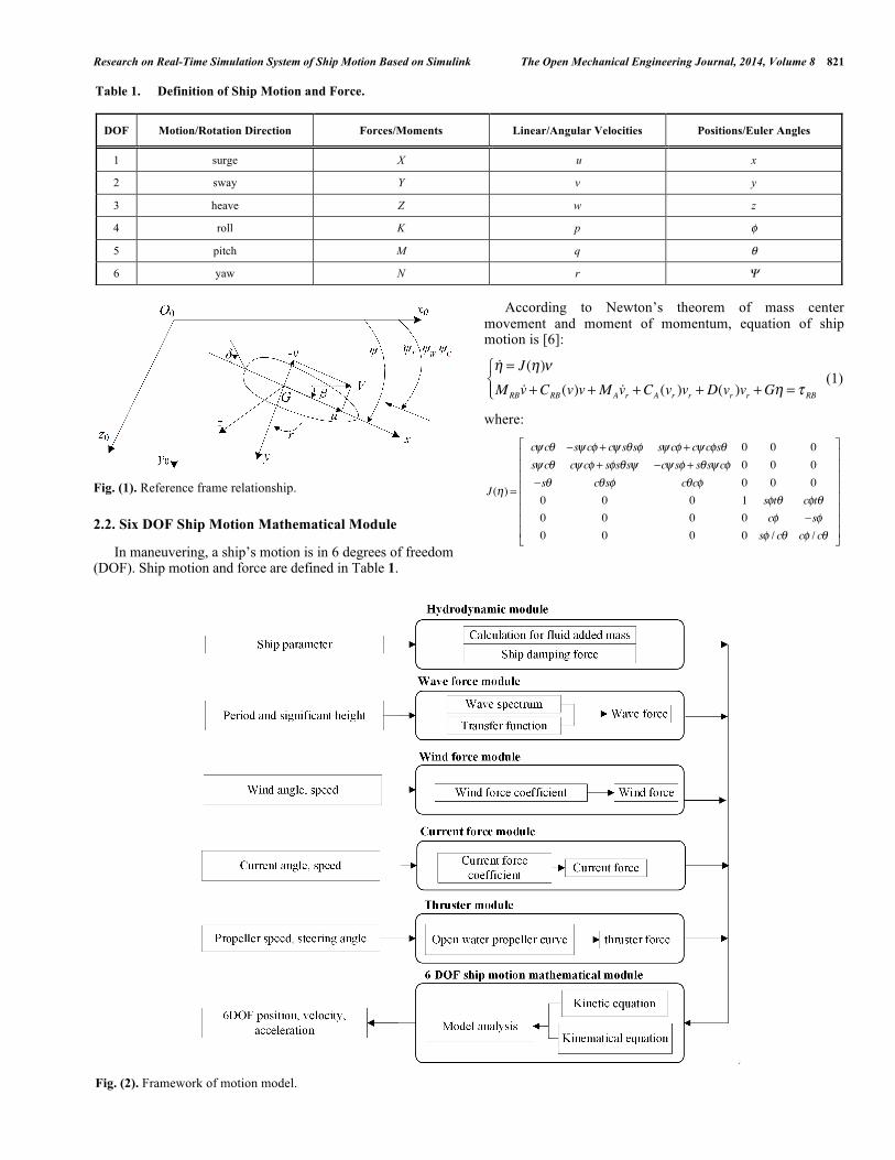
Gx axis. Ship motion model is divided into a main module (6 DOF ship motion mathematical module) and five component modules (hydrodynamic module, wave force module, wind force module, current force module and thruster module) as shown in Fig. (2).

Research on Real-Time Simulation System of Ship Motion Based on Simulink The Open Mechanical Engineering Journal, 2014, Volume 8 821

Fig. (1). Reference frame relationship.

2.2. Six DOF Ship Motion Mathematical Module

In maneuvering, a ship’s motion is in 6 degrees of freedom (DOF). Ship motion and force are defined in Table 1.

According to Newton’s theorem of mass center movement and moment of momentum, equation of ship motion is [6]:

!! = J(!)"MRB !v +CRB(v)v +MA !vr +CA(vr )vr + D(vr )vr +G! = # RB

$%&'

(1)

where:

J(!) =

c" c# $s" c% + c" s#s% s" c% + c" c%s# 0 0 0s" c# c" c% + s%s#s" $c" s% + s#s" c% 0 0 0$s# c#s% c#c% 0 0 00 0 0 1 s%t# c%t#0 0 0 0 c% $s%0 0 0 0 s% / c# c% / c#

&

'

((((((((

)

*

++++++++

Table 1. Definition of Ship Motion and Force.

DOF Motion/Rotation Direction Forces/Moments Linear/Angular Velocities Positions/Euler Angles

1 surge X u x

2 sway Y v y

3 heave Z w z

4 roll K p φ

5 pitch M q θ

6 yaw N r Ψ

Fig. (2). Framework of motion model.

822 The Open Mechanical Engineering Journal, 2014, Volume 8 Zan et al.

! = [x, y,z,",# ,$ ]T , ! = [u,v," , p,q,r]T ;

MRB is the rigid-body inertia matrix;

CRB is the Coriolis-centripetal matrix;

MA is the added mass inertia matrix;

CA(! r ) is the added mass Coriolis-centripetal matrix;

D(vr ) is the damping matrix

G is the stiffness matrix;

vr = v ! vc is the relative velocity;

! RB = [X,Y ,Z,K ,M ,N ]T is the environmental disturbance

from wind, waves and currents.

where: c(i) = cos(i),s(i) = sin(i)

2.3. Hydrodynamic Module

Added mass and damping coefficient are obtained by model tests, while lack of data of ship model empirical method is also practical.

2.3.1. Plane Added Mass Calculation

Zhou Zhao-ming applied multivariate regression analysis to Yuan Liang-cheng three spectrum, offering a method for estimating added mass of plane motion [7].

!11m

= 1100

[0.398 +11.97Cb (1+ 3.73dB)" 2.89Cb

LB

*(1+1.13 dB)+ 0.175Cb (

LB)2 (1+ 0.541 d

B)"1.107 L

BdB]

!22m

= 0.882 " 0.54Cb (1"1.6dB)" 0.156 L

B(1" 0.673Cb )

+0.826 dBLB(1" 0.678 d

B)" 0.638 d

BLB(1" 0.669 d

B)

!66mL2

= 1100

[33" 76.85Cb (1" 0.784Cb )

+3.43 LB(1" 0.63Cb )]"1.107

LBdB]

(2)

where:

m is the ship mass

Cb is the block coefficient

d is the ship draught

L is the ship length

B is the ship breadth

2.3.2. Rolling Added İnertial Moment Calculation

Rolling added inertial moment can be calculated as [8]:

Ix + !44 ="g#$

2 (3)

where:

! is displacement;

g is acceleration of gravity;

!" is inertial radius for rolling with consideration of added mass, as a result of product of breadth B and empirical coefficient c . For passenger ships, c＝0.40～0.435. For cargo ship, when full load c＝0.32～0.35, then in ballast c＝0.37～0.40. According to the requirement of Japanese stability norm, for full form ship, Formula (4) is the method for calculation:

c = 0.3725 + 0.0227 Bd! 0.0043 L

100 (4)

For fine form ship, it is:

c = 0.3085 + 0.0227 Bd! 0.0043 L

100 (5)

2.3.3. Heave Added Mass and Pitch Added Inertial Moment Calculation

Heave added mass and pitch added inertial moment can be estimated by F. Tasai’s empirical method:

!33 = 0.8B2d

Cwm

!55 = 0.83B2d

Cp2 (0.25L)2m

"

#$$

%$$

(6)

where:

Cw is the waterplane coefficient;

Cp is the prismatic coefficient.

2.3.4. Plane-Motion Viscous Hydrodynamic Coefficient

Estimation for plane-motion viscous hydrodynamic force is obtained by [9]:

XN = X(u)+ Xvvv2 + Xvrvr + Xrrr

2

YN = Yvv +Yrr +Yv v v v +Yv r v r +Yr r r r +Yvvrv2r +Yvrrvr

2

NN = Nvv + Nrr + Nvv v v + Nr r r r + Nvvrv2r + Nvrrvr

2

!

"##

$##

(7)

X(u) is resistance when the ship is in direct route; Xvv , Xvr , Xrr are derivatives of longitudinal nonlinear hydrodynamic force; Yv , Yr , Yv v , Yv r , Yr r , Yvvr , Yvrr are derivatives of

transverse linear and nonlinear hydrodynamic force; and Nv , Nr , Nvv , Nr r , Nvvr , Nvrr are derivatives of heading linear

and nonlinear hydrodynamic force.

2.3.5. Estimation for Rolling Damping Moment

Roll damping moment follows linear relation with roll angular velocity, L !! is rolling damping coefficient while rolling angle is small. The method for estimation is :

L !! = µ! (Ix + "44 ) # $ #GM (8)


where:

GM is the metacentric height;

µ! is the non-dimensional attenuation coefficient.

2.3.6. Heaving and Pitching Viscous Hydrodynamic Calculation

Heave viscous hydrodynamic coefficient ZV is:

ZV = !Z !z !z ! Zzz ! Z !!" !!" ! Z !" !" ! Z"" (9)

Pitch viscous hydrodynamic moment MV is:

MV = !M !"!" !M"" !M !!z!!z !M !z !z !Mzz (10)

Combining F. Tasai’s empirical method (9) with hydrodynamic derivatives in (10) [10]. Heave hydrodynamic derivative:

Z !z = N x( )dx = 5.4Cw

Cp

B2d

! 4.7"

#$$

%

&''

(gLL)

Zz = *gAwZ !!+ = !,33xG - 0

Z !+ = ! N x( )xdx + ,33 ! ,11( )uL)

= *g./GML

u+ ,33 ! ,11( )u

Z+ = u N x( )dx = uZ !zL)

0

1

222222

3

222222

(11)

Pitch hydrodynamic derivative:

M !! = N x( )x2 dxL" = 0.08#L

2

gL$ B2d

M! = %g&GML

M !!z = '(11xG ) 0

M !z = ' N x( )xdx ' (33 ' (11( )uL"

= %g&GML

u' (33 ' (11( )u

Mz = %gAwx f

*

+

,,,,,,

-

,,,,,,

(12)

where:

Cw is waterplane coefficient;

Cp is prismatic coefficient;

! is density of sea water;

g is gravitational acceleration;

GML is longitudinal metacentric height;

Aw is waterplane area;

x f is x value of center of floatation.

2.4. Wind Force Module

When a ship is in motion in the sea, effect of wind on the area of ship which is above waterline, leads to heading

deviation and difficulties for manipulation. When sailing in the harbor at low speed, the impact of wind on the ship's steering is particularly obvious, making maneuvering more complicated. So, calculation for wind force plays an important role in accuracy of simulation.

Wind speed above ocean surface is termed as and

wind angle is . Wind speed and wind angle defined in earth-fixed reference fame are also called true wind speed and true wind angle. Definition of true wind angle is: northern wind is 0 degree, eastern wind is 90 degree, and arrangement of is from 0 to 360. Wind speed and wind angle observed in body-fixed reference fame are relative wind speed and relative wind angle. Relative wind speed is termed as , with the value of wind from portside being positive.

Relationship of turn wind speed UT , ship speed V and relative wind speed UR is:

!UR =

!UT !

!V (13)

Rotating the body-fixed frame we get

uR = !u !UT cos("T !# )vR = !v !UT sin("T !# )

(14)

where: uR,vR are the values of UR on x, y axis in body-fixed frame, UR

2 = uR2 + vR

2 .

İn the body-fixed frame, value of wind angle ! R from portside is positive, so:

! R = arctan("vRuR)+ sgn(# ,vR ) uR > 0

! R = arctan("vRuR) uR < 0

$

%

&&

'

&&

(15)

Wind forces and moments acting on ships are calculated by (16):

XWIND = 0.5!aAfUR2Cwx (" R )

YWIND = 0.5!aAsUR2Cwy(" R )

NWIND = 0.5!aAsLOAUR2Cwn (" R )

#

$%%

&%%

(16)

where:

!a = 1.204kg /m3 is the air density

LOA is the overall length

Af ,As are areas of longitudinal and lateral projection above water surface.

Cwx (! R ),Cwy(! R ),Cwn (! R ) are coefficients of longitudinal and lateral wind resistance and rolling moment, obtained by empirical equations or wind tunnel tests [11, 12].

2.5. Current Force Module

Similar to wind, sea current forces and moments are calculated by (17):

TU

TΨ TU TΨ

TΨ

RU


Xcurrent = 0.5!Uc2Ac

fCcx (" )Ycurrent = 0.5!Uc

2AcsCcy(" )

Ncurrent = 0.5!Uc2Ac

sLOACcn (" )

#

$%

&%

(17)

where:

!a = 1.025 "103kg /m3 is water density

LOA is the overall length

Acf ,Ac

s are areas of longitudinal and lateral projection below water surface.

Ccx (! ),Ccy(! ),Ccn (! ) are coefficients of longitudinal and lateral current resistance and rolling moment, obtained by wind tunnel tests.

2.6. Wave Force Module

In order to meet real-time simulation, for obtaining value of wave force, hydrodynamic software is applied to calculate wave force transfer function in different ship speed, heading angle and wave frequency [13]. In real-time simulation, value of wave force is calculated in each step by interpolation algorithm:

Fwave = H (! ," )# (! ," , x, y,t) (18)

where:

H (! ," ) is wave force transfer function as a function of wave frequency! ship heading angle! ;

! (" ,# , x, y) is wave height.

Since real sea wave is extremly irregular and wave height, wave length and period are randomly varying, equation for regular wave is invalid. Assuming that irregular wave! (" ,# , x, y) is composed of large number of unit waves with various wavelengths, wave amplitudes and random phases, irregular wave is expressed as [14, 15]:

! (" ,# , x, y,t) = Ai, jj=1

m

$i=1

n

$ cos(kix cos# j

+kiysin# j %" it +& ) (19)

For utilizing spectrum analysis to forecast the performance of ship in irregular waves, firstly, wave/wind spectrum density is estimated of voyage areas. Researchers have proposed a variety of ocean wave spectrum expressions based on a number of observational and theoretical works, for example, Bretschneitder spectrum, Pierson-Moskowitz spectrum, ITTC parameter spectrum, JONSWAP spectrum and Torsethaugen spectrum. In this paper, a double-parameter spectrum method which is recommended by ITTC and ISSC is applied. This spectrum is applicable to fully developed waves, developing waves and waves with swell:

S(! ) = 173H1/32

T14! 5 exp " 691

T14! 4

#$%

&'(

(20)

where:

H1/3 is one-third significant wave height;

T1 is the spectral centroid period, close to average period from observation where T1 = 2!m0 /m1 ; it can also be termed as peak spectral period, in relation with peak spectral period: T0 = 1.2965T1 ;

! is angular frequency.

Lee carried out statistics for sea state of Atlantic and North Pacific in 1985, offering values of significant height, spectral peak period and wind speed and possibility for each sea state. More details are listed in reference [16]. Since ITTC double-parameter spectrum is 1-D, but real sea wave is 3-D, energy is distributed within a broad range of frequencies and directions, in order to characterize the wave as being direction-dependent. ITTC recommends a direction spectral function:

D(! ) = 2"cos2 !

2#$%

&'( ! ) "

2 (21)

If frequency distribution and direction distribution of wave energy are independent and linear, distribution of wave energy can be termed by product of sea wave spectral function and direction spectral function:

Ai, j = S(! )D(" ) =173H1/3

2

T14! 5 exp # 691

T14! 4

$%&

'()

* 2+cos2 "

2$%&

'()

(22)

2.7. Thruster Module

A model is applied to calculate the thruster of propeller T and torque Q in real conditions:

T = (1! t p )"n2D4KT

Q = (1! t p )"n2D5KQ

Jp = (1!# p )U / (nD)

$

%&&

'&&

(23)

where:

J is the advance coefficient;

wp is the wake current coefficient;

t p is the thrust deduction coefficient;

n is the propeller speed;

D is the propeller diameter;

KT ,KQ is the thrust coefficient and torque coefficient, obtained by propeller test in open water;

3. RAPID DEVELOPMENT FOR MOTON SIMU- LATION SYSTEM

For real-time communication, firstly mutual transmission is achieved by UDP protocol. A real-time


Fig. (3). The flow chart of real-time simulation system.

Fig. (4). UDP communication model development.


communication module by S-Function is established and the module is added into Simulink model. As a result, controlling real-time calculation for simulation data is achieved. Fig. (3) shows the flow chart of real-time simulation system.

4. UDP COMMUNICATION

UDP communication module contains a data receiver module and a data transmission module. After receiving real-time control data from simulation control system, motion simulation system analyzes the data packet and then carries out ship motion calculation and finally, data transmission module transfers the data of ship motion to visual simulation system. Fig. (4) represents UDP communication module in Simulink.

5. RESULTS AND DISCUSSION

Inputting parameters into ship simulation control system, wave average period is T = 7.2s , wave significant height is H1/3 = 2.5m , wind speed Uwind = 18kn , wave angle and wind angle both are ! = 45° , speed of left/right propeller is n = 180rpm . When simulation time is 800 s, steering angle changes to ! = 15° . Figs. (5-7) show the results of motion simulation.

Fig. (5). Heave angle curve.

Fig. (6). Roll angle curve.

Fig. (7). Pitch angle curve.

A ship maintains direct sailing in waves in [0s,800s] , at peak value of heave in 0.18 m, while peak value of roll angle is 1 degree, and peak value of pitch angle is 0.25 degree. At800s , ship begins to change steering angle, peak value of heave increases to approximately 0.3 m, peak value of rolling increases to 2.5 degree, with slight change occurring on the pitch. Fig. (8) is the final result of simulation shown in visual system:

Fig. (8). Visual scene display.

CONCLUSION

In this paper, a project ship was taken as a sample, and a method based on Simulink was introduced for developing a real-time simulation system. After verifying real-time communication, visual-refresh rate of visual system reached 100 HZ, fully satisfying the requirement of visual real-time. This method avoids tedious work for manually changing codes, eliminates the process of compiling codes for communication and real-time simulation control. It also greatly facilitates the development and integration of the system, shortening the process of developing real-time simulation system.

CONFLICT OF INTEREST

The authors confirm that this article content has no conflict of interest.

0 500 1000 1500 2000-‐ 0. 4

-‐ 0. 3

-‐ 0. 2

-‐ 0. 1

0

0. 1

0. 2

0. 3

0. 4

Ti me( s )

Heav

e(m)

0 500 1000 1500 2000-‐ 3

-‐ 2. 5

-‐ 2

-‐ 1. 5

-‐ 1

-‐ 0. 5

0

0. 5

1

1. 5

Ti me( s )

Roll

(deg

)

0 500 1000 1500 2000-‐ 0. 4

-‐ 0. 3

-‐ 0. 2

-‐ 0. 1

0

0. 1

0. 2

0. 3

Ti me( s )

Pitc

h(de

g)


ACKNOWLEDGEMENTS

This work is supported by the National Science and Technology Major Project of the Ministry of Science and Technology of China (No. 2011ZX05027-002), China Scholarship Council and the Technology Project of China National Offshore Oil Corporation (No. CN00C-KJ 125 ZDXM 05 GC 00 GC 2013-04).

REFERENCES

[1] Z. Tao, "Research on network communication between Simulink and VC++ based on S-function," Modern Electronics Technique, vol. 36, no. 13, pp. 108-111, 2013.

[2] C. Salzmann, D. Gillet, and P. Huguenin, "Introduction to real-time control using LabVIEWTM with an application to distance learning," International Journal of Engineering Education, vol. 16, no. 5, pp. 372-384, 2000.

[3] B. Netten, and H. Wedemeijer, "Testing cooperative systems with the MARS simulator," In: Proc. Intelligent Transportation Systems (ITSC), 2010 13th International IEEE Conference on, IEEE, pp. 186-191, 2010.

[4] A. M. Abdullah, and M. A. Dia, "Creating Real-Time operation System Based on xPC Target Kernel," International Journal of Recent Technology and Engineering, vol. 2, no. 4, pp. 143, 2013.

[5] SNAME, "The Society of Naval Architects and Marine Engineers," Nomenclature for Treating the Motion of a Submerged Body Through a Fluid. In: Technical and Research Bulletin No. 1-5., New York, USA 1950.

[6] T. I. Fossen, "Handbook of marine craft hydrodynamics and motion control," Wiley, 2011.

[7] Z. Zhou, Z. Sheng and W. Fen, "Multipurpose cargo handling forecast calculation," Ship Engineering, no. 6, pp. 21-29+36+24, 1983.

[8] J. Li, "Ship seakeeping", Harbin Shipbuilding Engineering Institute Press, Harbin, 1992.

[9] X. Jia, and Y. Yang, "Ship motion mathematical model", Dalian Maritime University Press: Dalian, 1999.

[10] F. Tasai, "On the Damping Force and Added Mass of Ships Heaveing and Pitching. ", Shipbuilders' Association Proceedings, vol. 105, pp. 47-56, 1959.

[11] T. I. Fossen, "How to Incorporate Wind, Waves and Ocean Currents in the Marine Craft Equations of Motion," IFAC MCMC'12, 2012.

[12] M. R. Haddara, and S. C. Guedes, "Wind loads on marine structures," Marine Structures, vol. 12, no. 3, pp. 199-209, 1999.

[13] Z. Chuang, and S. Steen, "Speed loss due to seakeeping and maneuvering in zigzag motion," Ocean Engineering, vol. 48, pp. 38-46, 2012.

[14] Z.B. Sheng, and Y. Z. Liu, "Principle of ship," Shanghai Jiao Tong University Press: Shanghai, 2004.

[15] Y. F. Zan, H. D. Zhi, L. Song, and W. Sun, "The Numerical Simulation Research of Three Dimensional Irregular Wave Based on Wave Spectrum", Applied Mechanics and Materials, vol. 397, pp. 643-647, 2013.

[16] W. T. Lee, S. L. Bales, and S. Sowby, "Standardized wind and wave environments for North Pacific Ocean Areas," DTIC Document, No. DTNSRDC/SPD-0919-02, 1985.

Received: December 8, 2014 Revised: December 15, 2014 Accepted: December 16, 2014 © Zan et al.; Licensee Bentham Open.

This is an open access article licensed under the terms of the Creative Commons Attribution Non-Commercial License (http://creativecommons.org/licenses/by-nc/4.0/) which permits unrestricted, non-commercial use, distribution and reproduction in any medium, provided the work is properly cited.

research on real-time simulation system of ship motion

Documents