research, development and technology transfer …model development of geosynthetic reinforced...
TRANSCRIPT

Mechanistic-Empirical Modeling and Design Model Development Final Report S.W. Perkins
Department of Civil Engineering, Montana State University – Bozeman, Bozeman, Montana 59717 i
MECHANISTIC-EMPIRICAL MODELING AND DESIGN MODEL DEVELOPMENT OF GEOSYNTHETIC
REINFORCED FLEXIBLE PAVEMENTS: FINAL REPORT
FHWA/MT−01−002/99160−1A
Final Report
Prepared for the STATE OF MONTANA
DEPARTMENT OF TRANSPORTATION RESEARCH, DEVELOPMENT AND TECHNOLOGY TRANSFER PROGRAM
in cooperation with the U.S. DEPARTMENT OF TRANSPORTATION
FEDERAL HIGHWAY ADMINISTRATION and the
Idaho, Kansas, Minnesota, New York, Texas, Wisconsin and Wyoming Departments of Transportation
and the Western Transportation Institute at Montana State University
October 1, 2001
Prepared by
Dr. Steven W. Perkins Associate Professor
Department of Civil Engineering Western Transportation Institute
Montana State University – Bozeman Bozeman, Montana 59717
Office Telephone: 406-994-6119 Fax: 406-994-6105
E-Mail: [email protected]
ii
TECHNICAL REPORT STANDARD PAGE 1. Report No. FHWA/MT−01−002/99160−1A
2. Government Accession No.
3. Recipient's Catalog No.
5. Report Date October 1, 2001
4. Title and Subtitle Mechanistic-Empirical Modeling and Design Model Development of Geosynthetic Reinforced Flexible Pavements: Final Report
6. Performing Organization Code MSU G&C #428573
7. Author Steven W. Perkins, Ph.D., P.E.
8. Performing Organization Report No. 10. Work Unit No.
9. Performing Organization Name and Address Department of Civil Engineering 205 Cobleigh Hall Montana State University Bozeman, Montana 59717
11. Contract or Grant No.
99160
13. Type of Report and Period Covered
Final: October 1, 1998 – October 1, 2001
12. Sponsoring Agency Name and Address Montana Department of Transportation Research Section 2701 Prospect Avenue P.O. Box 201001 Helena, Montana 59620-1001
14. Sponsoring Agency Code 5401
15. Supplementary Notes
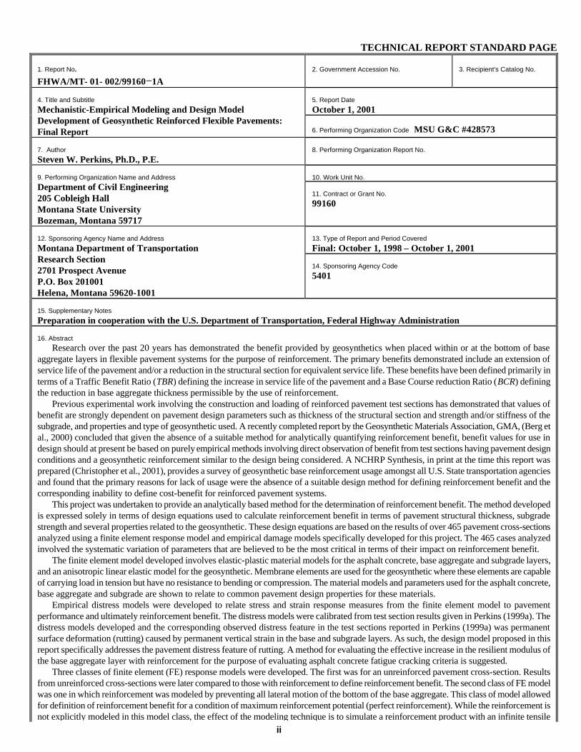
Preparation in cooperation with the U.S. Department of Transportation, Federal Highway Administration 16. Abstract
Research over the past 20 years has demonstrated the benefit provided by geosynthetics when placed within or at the bottom of base aggregate layers in flexible pavement systems for the purpose of reinforcement. The primary benefits demonstrated include an extension of service life of the pavement and/or a reduction in the structural section for equivalent service life. These benefits have been defined primarily in terms of a Traffic Benefit Ratio (TBR) defining the increase in service life of the pavement and a Base Course reduction Ratio (BCR) defining the reduction in base aggregate thickness permissible by the use of reinforcement.
Previous experimental work involving the construction and loading of reinforced pavement test sections has demonstrated that values of benefit are strongly dependent on pavement design parameters such as thickness of the structural section and strength and/or stiffness of the subgrade, and properties and type of geosynthetic used. A recently completed report by the Geosynthetic Materials Association, GMA, (Berg et al., 2000) concluded that given the absence of a suitable method for analytically quantifying reinforcement benefit, benefit values for use in design should at present be based on purely empirical methods involving direct observation of benefit from test sections having pavement design conditions and a geosynthetic reinforcement similar to the design being considered. A NCHRP Synthesis, in print at the time this report was prepared (Christopher et al., 2001), provides a survey of geosynthetic base reinforcement usage amongst all U.S. State transportation agencies and found that the primary reasons for lack of usage were the absence of a suitable design method for defining reinforcement benefit and the corresponding inability to define cost-benefit for reinforced pavement systems.
This project was undertaken to provide an analytically based method for the determination of reinforcement benefit. The method developed is expressed solely in terms of design equations used to calculate reinforcement benefit in terms of pavement structural thickness, subgrade strength and several properties related to the geosynthetic. These design equations are based on the results of over 465 pavement cross-sections analyzed using a finite element response model and empirical damage models specifically developed for this project. The 465 cases analyzed involved the systematic variation of parameters that are believed to be the most critical in terms of their impact on reinforcement benefit.
The finite element model developed involves elastic-plastic material models for the asphalt concrete, base aggregate and subgrade layers, and an anisotropic linear elastic model for the geosynthetic. Membrane elements are used for the geosynthetic where these elements are capable of carrying load in tension but have no resistance to bending or compression. The material models and parameters used for the asphalt concrete, base aggregate and subgrade are shown to relate to common pavement design properties for these materials.
Empirical distress models were developed to relate stress and strain response measures from the finite element model to pavement performance and ultimately reinforcement benefit. The distress models were calibrated from test section results given in Perkins (1999a). The distress models developed and the corresponding observed distress feature in the test sections reported in Perkins (1999a) was permanent surface deformation (rutting) caused by permanent vertical strain in the base and subgrade layers. As such, the design model proposed in this report specifically addresses the pavement distress feature of rutting. A method for evaluating the effective increase in the resilient modulus of the base aggregate layer with reinforcement for the purpose of evaluating asphalt concrete fatigue cracking criteria is suggested.
Three classes of finite element (FE) response models were developed. The first was for an unreinforced pavement cross-section. Results from unreinforced cross-sections were later compared to those with reinforcement to define reinforcement benefit. The second class of FE model was one in which reinforcement was modeled by preventing all lateral motion of the bottom of the base aggregate. This class of model allowed for definition of reinforcement benefit for a condition of maximum reinforcement potential (perfect reinforcement). While the reinforcement is not explicitly modeled in this model class, the effect of the modeling technique is to simulate a reinforcement product with an infinite tensile
iii
stiffness and an infinitely stiff geosynthetic/aggregate shear interface. Results from the second class of FE model were compared to those of the unreinforced pavement to develop equations describing reinforcement benefit for the case of perfect reinforcement. These equations account for variations in asphalt concrete and base aggregate thickness, and subgrade strength.
The influence of geosynthetic properties was evaluated by creating a third class of FE model. In this model, the geosynthetic was explicitly accounted for by including a geosynthetic sheet, modeled with membrane elements, between the base aggregate and subgrade layer. Results from cases using this FE model were used to develop expressions for reduction factors applied to benefit seen for the cases of perfect reinforcement to account for the geosynthetic material properties varied in the study.
The anisotropic, linear-elastic material model used for the geosynthetic allowed for the variation of four basic geosynthetic material properties. These properties included the elastic modulus in the strong and weak principal directions of the material, the in-plane Poisson’s ratio and the in-plane shear modulus. The design method is based on the use of a secant tensile modulus measured at 2 % axial strain from a wide-width tension test, ASTM D 4595 (ASTM, 2001a), for later definition of the elastic modulus. Reinforcement benefit is seen to be most heavily influenced by these two parameters (i.e. elastic modulus in the strong and weak principal material directions).
Geosynthetic in-plane Poisson’s ratio and shear modulus are most likely related to the type and structure of the geosynthetic. Test methods and reported values for these parameters are not currently available. As such, the design method does not allow for the specific input of these two parameter values. Rather the method requires that one of two benefit reduction factors be specified for each material parameter. The two choices for benefit reduction factors correspond to good or poor values for these material parameters. Calibration of the design model from test section results using two geogrid and one geotextile product has resulted in recommended values for these products, which serve as a starting point when selecting values for other products.
The influence of base aggregate-geosynthetic shear interaction is accounted for empirically by calibration of the design method against results from published test sections, where this influence is also expressed in terms of a benefit reduction factor. Since the design method was calibrated from test section results using two types of geosynthetics, reduction factors for interface shear were developed for each type of material.
Design equations were developed for reinforcement benefit defined in terms of a TBR, BCR or a combination of the two. Furthermore, benefit defined in terms of TBR and/or BCR was broken into components associated with reinforcement effects on the subgrade, reinforcement effects on the base aggregate, and combined effects on the total pavement system. Since distress models were developed for effects in the subgrade and effects in the base aggregate layer, calibration of the design model required that separate benefit values be determined. The generally conservative nature of the design method suggests that benefit values for the total system be used.
The design model was calibrated and verified by comparison to test section results reported in Perkins (1999a), where these results were analyzed to derive experimental definitions of benefit for reinforcement effects in the base aggregate and subgrade layers. Further validation of the model was accomplished by comparison to other test section results available in the literature as summarized in Berg et al. (2000).
The design model is shown to provide generally conservative estimates of reinforcement benefit when compared to available test section results. The model is shown to be sensitive to design parameters of asphalt concrete and base aggregate thickness, subgrade strength, geosynthetic tensile modulus and tensile modulus ratio and other geosynthetic elastic material model properties. The model tends to show variations of benefit with these design parameters that are consistent with general application guidelines developed in Berg et al. (2000). Several examples are described to illustrate the use of the model and to illustrate the construction and life-cycle cost benefit that can result from the use of reinforcement.
This report provides a detained description of the finite element response model, the material models used in the FE model, calibration of the material models and how these models relate to commonly used pavement layer material models, and the steps followed to develop the design model. Limitations for use of the model are described in Sections 7.8 and Appendix B. Section 8 of the report provides a summary of the equations developed for the design model and provides suggestions for how the design model can be extended to situations not specifically addressed in the project. The design equations have been programmed into a spreadsheet program that is also described in Section 8 and can be downloaded from the following URL: http://www.mdt.state.mt.us/departments/researchmgmt/grfp/grfp.html. Appendix B of the report provides a summary of the design model as it relates to its use in practice. The material provided in Appendix B constitutes a design guideline based on the design model developed in this project. Examples are provided in Appendix B to illustrate the use of the design model and the cost-benefit for the examples given. 17. Key Words Pavements, Highways, Geogrid, Geotextile, Geosynthetic, Reinforcement, Base Course, Finite Element Model, Numerical Modeling, Design, Montana
18. Distribution Statement Unrestricted. This document is available through the National Technical Information Service, Springfield, VA 21161.
19. Security Classif. (of this report) Unclassified
20. Security Classif. (of this page)
Unclassified
21. No. of Pages 170
22. Price

Mechanistic-Empirical Modeling and Design Model Development Final Report S.W. Perkins
Department of Civil Engineering, Montana State University – Bozeman, Bozeman, Montana 59717 iv
PREFACE DISCLAIMER The opinions, findings and conclusions expressed in this publication are those of the author and not necessarily those of the Federal Highway Administration, the Idaho, Kansas, Minnesota, New York, Montana, Texas, Wisconsin and Wyoming Departments of Transportation or the Western Transportation Institute. ALTERNATE FORMAT STATEMENT MDT attempts to provide reasonable accommodations for any known disability that may interfere with a person participating in any service, program or activity of the department. Alternative accessible formats of this document will be provided upon request. For further information, call (406) 444-7693 or TTY (406) 444-7696. NOTICE The authors, the State of Montana and the Federal Highway Administration do not endorse products or manufacturers. Trade and manufacturers names appear herein solely because they are considered essential to the object of the report.

Mechanistic-Empirical Modeling and Design Model Development Final Report S.W. Perkins
Department of Civil Engineering, Montana State University – Bozeman, Bozeman, Montana 59717 v
ACKNOWLEDGEMENTS The author gratefully recognizes the generous financial and technical support of the Montana, Idaho, Kansas, Minnesota, New York, Texas, Wisconsin and Wyoming Departments of Transportation and the Western Transportation Institute at Montana State University. The technical review provided by Mr. William Vischer of the Region 1 Engineering USDA Forest and formally of the Montana Department of Transportation provided significant substance to the report. The technical contribution of Mr. Yan Wang and Dr. Mike Edens is gratefully recognized. The Amoco Fabrics and Fibers Company and Tensar Earth Technologies, Incorporated graciously donated geosynthetic materials for preceding projects leading up to this work. They and the Tenax Corporation provided geosynthetic product information used in this report. Dr. Muralee Muraleetharan of the University of Oklahoma and Dr. Kim Mish of Lawrence Livermore National Laboratory generously provided source code and support for development of a user defined material model.

Mechanistic-Empirical Modeling and Design Model Development Final Report S.W. Perkins
Department of Civil Engineering, Montana State University – Bozeman, Bozeman, Montana 59717 vi
TABLE OF CONTENTS LIST OF TABLES viii LIST OF FIGURES x CONVERSION FACTORS xi EXECUTIVE SUMMARY xii 1.0 INTRODUCTION 1 2.0 LITERATURE REVIEW 2 2.1 Geosynthetic Reinforced Flexible Pavement Performance 2
2.2 Design Solutions for Geosynthetic Reinforced Pavements 9 2.3 Summary of an Existing Recommended Standard of Practice 13
2.4 Mechanistic-Empirical Modeling of Flexible Pavements 15 2.5 Modeling of Geosynthetic Reinforced Pavements 16 2.6 Tension and Interface Testing of Geosynthetics 21
3.0 PRIOR TEST SECTION WORK 21 3.1 Test Sections Constructed 22 3.1.1 Test Box and Loading Apparatus 22 3.1.2 Pavement Layer Materials 24 3.1.3 Instrumentation 27 3.1.4 As-Constructed Pavement Layer Properties 28 3.2 Summary of Results and Data Analysis 30 4.0 PAVEMENT LAYER MATERIAL MODELS AND CALIBRATION TESTS 39
4.1 Asphalt Concrete 40 4.2 Base Aggregate and Subgrade 43 4.3 Geosynthetics 52
5.0 PAVEMENT TEST FACILITY FINITE ELEMENT MODEL 56 5.1 Unreinforced FE Model 57 5.2 Perfect Reinforced FE Model 59 5.3 Geosynthetic Reinforced FE Model 60 5.4 Response Parameters and Extension to Reinforcement Benefits 60
6.0 PARAMETRIC STUDY AND RESULTS 65 6.1 Variation of Parameters for Perfect Reinforced Models 66 6.2 Variation of Parameters for Geosynthetic Reinforced Models 76
6.2.1 Parameters to Examine Effect of Reinforcement Modulus 76 6.2.2 Parameters to Examine Effect of Reinforcement Modulus Anisotropy 78 6.2.3 Parameters to Examine Effect of Poisson’s Ratio and Shear Modulus 79
7.0 DESIGN MODEL DEVELOPMENT 80 7.1 Design Equations for Perfect Reinforcement 80 7.1.1 Equations for TBR for Perfect Reinforcement 80 7.1.2 Equations for BCR and TBR/BCR Combinations Perfect Reinforcement 84 7.2 Influence of Geosynthetic Isotropic Elastic Modulus on TBR 91 7.2.1 Equations for TBRS 92 7.2.2 Equations for TBRB 96 7.3 Influence of Geosynthetic Modulus Anisotropy on TBR 97
7.4 Influence of Geosynthetic Poisson’s Ratio and Shear Modulus on TBR 98 7.5 Influence of Interface Properties on TBR 99

Mechanistic-Empirical Modeling and Design Model Development Final Report S.W. Perkins
Department of Civil Engineering, Montana State University – Bozeman, Bozeman, Montana 59717 vii
7.6 Calibration of Design Model 100 7.7 Comparison of Desgin Model to Other Published Results 102 7.8 Discussion of Design Model 106 8.0 DESIGN MODEL SUMMARY 108 8.1 Design Input 109 8.2 Design for a TBR for BCR = 0 110 8.3 Design for a BCR for TBR = 1 112 8.4 Design for a TBR/BCR Combination 114 8.5 Adjustment of Structural Layer Coefficients 115 8.6 Accounting for Subbase Aggregate Layers 116 8.7 Evaluating Asphalt Fatigue Cracking Criteria 116 8.8 Design Model Software Program 118 9.0 INCORPORATION OF DESIGN MODEL INTO A STANDARD OF PRACTICE 119 10.0 CONCLUSIONS 119 11.0 REFERENCES 122 APPENDIX A: NOTATION 127 APPENDIX B: DESIGN GUIDE 132
B.1.0 INTRODUCTION 132 B.2.0 APPLICATION BACKGROUND 132 B.3.0 DESIGN MODEL BACKGROUND 133 B.4.0 REINFORCEMENT BENEFIT DEFINITIONS 134 B.5.0 DESIGN MODEL 135
B.5.1 Design Model Input 135 B.5.2 Design Model Output 140 B.5.3 Design Model Input Limitations 142
B.6.0 DESIGN STEPS 142 B.7.0 DESIGN EXAMPLES 144
B.7.1 Illustrative Example 144 B.7.2 Project Example 151
Mechanistic-Empirical Modeling and Design Model Development Final Report S.W. Perkins
Department of Civil Engineering, Montana State University – Bozeman, Bozeman, Montana 59717 viii
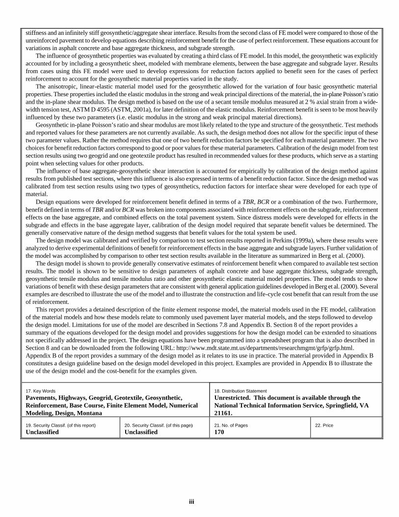
LIST OF TABLES Table 2.1.1 Variables influencing reinforcement effect (after Berg et al., 2000). 6 Table 2.1.2 Qualitative application guidelines for geosynthetic type
(after Berg et al., 2000). 7
Table 2.2.1 Summary of empirical design methods for geosynthetic reinforced pavements (after Berg et al. 2000).
9
Table 2.5.1 Summary of finite element studies of geosynthetic reinforced pavements. 17 Table 3.1.1 Comparison test section variables. 22 Table 3.1.2 Geosynthetic material properties. 26 Table 3.1.3 As-constructed asphalt concrete properties. 29 Table 3.1.4 As-constructed base course properties. 29 Table 3.1.5 As-constructed subgrade properties. 30 Table 3.1.6 Test section loading conditions. 30 Table 3.2.1 TBR’s for reinforced test sections at 12.5 mm permanent surface deformation.
37
Table 3.2.2 Total vertical strain at peak load for the first load cycle. 39 Table 4.1.1 Indirect tension resilient modulus test results. 43 Table 4.1.2 Material parameter values used for the asphalt concrete. 44 Table 4.2.1 Listing of bounding surface model material parameters. 48 Table 4.2.2 Calibrated bounding surface model parameters for test section materials. 50 Table 4.3.1 Geosynthetic material properties for biaxial loading. 53 Table 4.3.2 Geosynthetic apparent stiffness for biaxial loading. 54 Table 5.4.1 TBRS for reinforced test sections. 62 Table 6.1.1 AC thickness in parametric study. 67 Table 6.1.2 Base thickness in parametric study. 67 Table 6.1.3 Subgrade properties in parametric study. 68 Table 6.1.4 Response measures from unreinforced and perfect reinforced models. 70 Table 6.2.1 Parameters for geosynthetic material model to examine effect of reinforcement modulus.
77
Table 6.2.2 Pavement sections used to evaluate effect of reinforcement modulus. 77 Table 6.2.3 Parameters for geosynthetic material model to examine effect of reinforcement modulus anisotropy.
78
Table 6.2.4 Pavement sections used to evaluate effect of reinforcement modulus anisotropy.
79
Table 6.2.5 Parameters for geosynthetic material model to examine effect of reinforcement Poisson’s ratio and shear modulus.
79
Table 6.2.6 Pavement sections used to evaluate effect of reinforcement Poisson’s ratio and shear modulus.
80
Table 7.4.1 Reduction factors for reinforcement Poisson’s ratio and shear modulus. 99 Table 7.6.1 Summary input parameters for design model and test section comparisons. 102 Table 7.6.2 Summary output for design model and test section comparisons. 102 Table 7.7.1 Summary output for design model and test section comparisons. 104 Table 7.7.2 Summary output for design model and test section comparisons. 105 Table 8.1.1 Design model input parameters. 110 Table 8.1.2 Reduction factors for geosynthetic Poisson’s ratio and shear modulus. 110
Mechanistic-Empirical Modeling and Design Model Development Final Report S.W. Perkins
Department of Civil Engineering, Montana State University – Bozeman, Bozeman, Montana 59717 ix
Table B.5.1 Design model input parameters. 137 Table B.5.2 Material properties of geosynthetics used for design model development. 138 Table B.5.3 Design model parameters for geosynthetics. 138 Table B.5.4 Design model output parameters. 140 Table B.7.1 Flexible structural design module input for example 1. 144 Table B.7.2 Thickness designs for design options for example 1. 145 Table B.7.3 TBR and BCR values for design options for example 1. 145 Table B.7.4 Construction and rehabilitation dates and performance periods
for example 1. 149
Table B.7.5 Life-cycle cost analysis input parameters for example 1. 150 Table B.7.6 Pay items for example 1. 150 Table B.7.7 Total life-cycle costs for design options for example 1. 151 Table B.7.8 Flexible structural design module input for example 2. 153 Table B.7.9 Thickness designs for design options for example 2. 153 Table B.7.10 TBR and BCR values for design options for example 2. 153 Table B.7.11 Construction and rehabilitation dates and performance periods
for example 2. 154
Table B.7.12 Thickness designs for options 1, 2 and 4 for reconstruction at year 20. 155 Table B.7.13 Life-cycle cost analysis input parameters for example 2. 156 Table B.7.14 Pay items for example 2. 156 Table B.7.15 Total life-cycle costs for design options for example 2. 156
Mechanistic-Empirical Modeling and Design Model Development Final Report S.W. Perkins
Department of Civil Engineering, Montana State University – Bozeman, Bozeman, Montana 59717 x
LIST OF FIGURES Figure 2.1.1 Schematic illustration of base reinforcement mechanisms. 4Figure 2.1.2 Schematic illustration of combinations of TBR and BCR. 5Figure 3.1.1 Schematic Diagram of the pavement test facility. 23Figure 3.1.2 Input load pulse and corresponding load cell measurement. 24Figure 3.1.3 Grain size distribution of AC and base aggregate, and silty sand subgrade. 25Figure 3.1.4 CBR versus compaction moisture content for the clay subgrade. 27Figure 3.2.1 Permanent surface deformation versus load cycle (CS2, 5, 6, 7, 8, 11). 31Figure 3.2.2 Permanent surface deformation versus load cycle (CS9, 10). 31Figure 3.2.3 Permanent surface deformation versus load cycle (SSS1, 2, 3, 4). 32Figure 3.2.4 TBR for sections CS5, 6, 7 and 11 relative to section CS2. 32Figure 3.2.5 TBR for section CS10 relative to section CS9. 33Figure 3.2.6 Permanent vertical strain vs. depth in the subgrade for test section CS2. 34Figure 3.2.7 Permanent deformation of surface, base and subgrade layers - CS2. 35Figure 3.2.8 Calculated surface deformation curves for isolated reinforcement effects
on base and subgrade for test section CS11. 37
Figure 3.2.9 Measured dynamic strain versus depth and best fit line per Equation 3.2.1 for test section CS2.
38
Figure 3.2.10 Total vertical strain in top of the subgrade for the first load cycle versus number of load cycles to reach 12.5 mm of permanent surface deformation.
40
Figure 4.2.1 Schematic illustration of the bounding surface plasticity model. 45Figure 4.2.2 Predicted resilient modulus values from base aggregate
bounding surface model. 51
Figure 5.1.1 Finite element mode of unreinforced pavement test sections. 58Figure 5.4.1 Volume used for averaging bulk stress in the base aggregate layer. 63Figure 7.1.1 TBRS-PR versus SN for perfect reinforcement model cases. 81Figure 7.1.2 Identification of constants for Equations 7.1.2-7.1.9. 82Figure 7.1.3 TBRB-PR versus AC thickness (D1) for perfect reinforcement model cases. 83Figure 7.1.4 Remaining TBRS, TBRB, TBRT from finite element model and AASHTO equations.
88
Figure 7.2.1 Effect of geosynthetic isotropic elastic modulus on curves for TBRS-PR. 92Figure 7.2.2 Reduction factor for geosynthetic isotropic elastic modulus (RFGM)
for SN.1.6. 93
Figure 7.2.3 Reduction factor for geosynthetic isotropic elastic modulus (RFGM) for SN.3.3.
95
Figure 7.2.4 Slope m versus subgrade CBR. 95Figure 7.2.5 TBRB comparison from FE model and Equation 7.2.15. 97Figure B.5.1 Design model software program input selection boxes. 136Figure B.5.2 Design model software program output boxes. 140Figure B.7.1 Design model input for Geogrid A for example 1. 146Figure B.7.2 Design model input for Geogrid B for example 1. 147Figure B.7.3 Design model input for Geotextile for example 1. 148Figure B.7.4 Design model input for example 2. 152
Mechanistic-Empirical Modeling and Design Model Development Final Report S.W. Perkins
Department of Civil Engineering, Montana State University – Bozeman, Bozeman, Montana 59717 xi
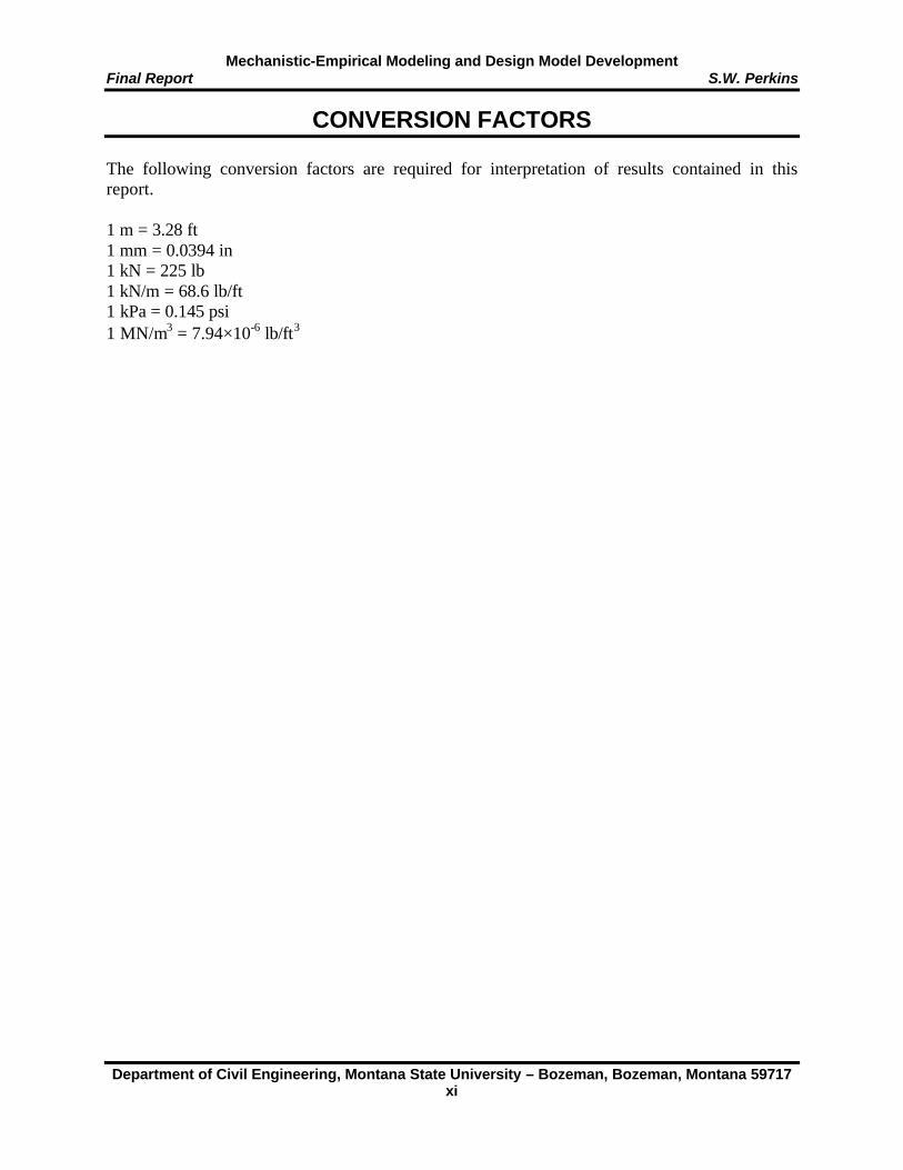
CONVERSION FACTORS The following conversion factors are required for interpretation of results contained in this report. 1 m = 3.28 ft 1 mm = 0.0394 in 1 kN = 225 lb 1 kN/m = 68.6 lb/ft 1 kPa = 0.145 psi 1 MN/m3 = 7.94×10⁻⁶ lb/ft3

Mechanistic-Empirical Modeling and Design Model Development Final Report S.W. Perkins
Department of Civil Engineering, Montana State University – Bozeman, Bozeman, Montana 59717 xii
EXECUTIVE SUMMARY
Research over the past 20 years has demonstrated the benefit provided by geosynthetics when placed within or at the bottom of base aggregate layers in flexible pavement systems for the purpose of reinforcement. The primary benefits demonstrated include an extension of service life of the pavement and/or a reduction in the structural section for equivalent service life. These benefits have been defined primarily in terms of a Traffic Benefit Ratio (TBR) defining the increase in service life of the pavement and a Base Course reduction Ratio (BCR) defining the reduction in base aggregate thickness permissible by the use of reinforcement.
Previous experimental work involving the construction and loading of reinforced pavement test sections has demonstrated that values of benefit are strongly dependent on pavement design parameters such as thickness of the structural section and strength and/or stiffness of the subgrade, and properties and type of geosynthetic used. A recently completed report by the Geosynthetic Materials Association, GMA, (Berg et al., 2000) concluded that given the absence of a suitable method for analytically quantifying reinforcement benefit, benefit values for use in design should at present be based on purely empirical methods involving direct observation of benefit from test sections having pavement design conditions and a geosynthetic reinforcement similar to the design being considered. A NCHRP Synthesis, in print at the time this report was prepared (Christopher et al., 2001), provides a survey of geosynthetic base reinforcement usage amongst all U.S. State transportation agencies and found that the primary reasons for lack of usage were the absence of a suitable design method for defining reinforcement benefit and the corresponding inability to define cost-benefit for reinforced pavement systems.
This project was undertaken to provide an analytically based method for the determination of reinforcement benefit. The method developed is expressed solely in terms of design equations used to calculate reinforcement benefit in terms of pavement structural thickness, subgrade strength and several properties related to the geosynthetic. These design equations are based on the results of over 465 pavement cross-sections analyzed using a finite element response model and empirical damage models specifically developed for this project. The 465 cases analyzed involved the systematic variation of parameters that are believed to be the most critical in terms of their impact on reinforcement benefit.
The finite element model developed involves elastic-plastic material models for the asphalt concrete, base aggregate and subgrade layers, and an anisotropic linear elastic model for the geosynthetic. Membrane elements are used for the geosynthetic where these elements are capable of carrying load in tension but have no resistance to bending or compression. The material models and parameters used for the asphalt concrete, base aggregate and subgrade are shown to relate to common pavement design properties for these materials.
Empirical distress models were developed to relate stress and strain response measures from the finite element model to pavement performance and ultimately reinforcement benefit. The distress models were calibrated from test section results given in Perkins (1999a). The distress models developed and the corresponding observed distress feature in the test sections reported in Perkins (1999a) was permanent surface deformation (rutting) caused by permanent vertical strain in the base and subgrade layers. As such, the design model proposed in this report specifically addresses the pavement distress feature of rutting. A method for evaluating the effective increase in the resilient modulus of the base aggregate layer with reinforcement for the purpose of evaluating asphalt concrete fatigue cracking criteria is suggested.

Mechanistic-Empirical Modeling and Design Model Development Final Report S.W. Perkins
Department of Civil Engineering, Montana State University – Bozeman, Bozeman, Montana 59717 xiii
Three classes of finite element (FE) response models were developed. The first was for an unreinforced pavement cross-section. Results from unreinforced cross-sections were later compared to those with reinforcement to define reinforcement benefit. The second class of FE model was one in which reinforcement was modeled by preventing all lateral motion of the bottom of the base aggregate. This class of model allowed for definition of reinforcement benefit for a condition of maximum reinforcement potential (perfect reinforcement). While the reinforcement is not explicitly modeled in this model class, the effect of the modeling technique is to simulate a reinforcement product with an infinite tensile stiffness and an infinitely stiff geosynthetic/aggregate shear interface. Results from the second class of FE model were compared to those of the unreinforced pavement to develop equations describing reinforcement benefit for the case of perfect reinforcement. These equations account for variations in asphalt concrete and base aggregate thickness, and subgrade strength.
The influence of geosynthetic properties was evaluated by creating a third class of FE model. In this model, the geosynthetic was explicitly accounted for by including a geosynthetic sheet, modeled with membrane elements, between the base aggregate and subgrade layer. Results from cases using this FE model were used to develop expressions for reduction factors applied to benefit seen for the cases of perfect reinforcement to account for the geosynthetic material properties varied in the study.
The anisotropic, linear-elastic material model used for the geosynthetic allowed for the variation of four basic geosynthetic material properties. These properties included the elastic modulus in the strong and weak principal directions of the material, the in-plane Poisson’s ratio and the in-plane shear modulus. The design method is based on the use of a secant tensile modulus measured at 2 % axial strain from a wide-width tension test, ASTM D 4595 (ASTM, 2001a), for later definition of the elastic modulus. Reinforcement benefit is seen to be most heavily influenced by these two parameters (i.e. elastic modulus in the strong and weak principal material directions).
Geosynthetic in-plane Poisson’s ratio and shear modulus are most likely related to the type and structure of the geosynthetic. Test methods and reported values for these parameters are not currently available. As such, the design method does not allow for the specific input of these two parameter values. Rather the method requires that one of two benefit reduction factors be specified for each material parameter. The two choices for benefit reduction factors correspond to good or poor values for these material parameters. Calibration of the design model from test section results using two geogrid and one geotextile product has resulted in recommended values for these products, which serve as a starting point when selecting values for other products.
The influence of base aggregate-geosynthetic shear interaction is accounted for empirically by calibration of the design method against results from published test sections, where this influence is also expressed in terms of a benefit reduction factor. Since the design method was calibrated from test section results using two types of geosynthetics, reduction factors for interface shear were developed for each type of material.
Design equations were developed for reinforcement benefit defined in terms of a TBR, BCR or a combination of the two. Furthermore, benefit defined in terms of TBR and/or BCR was broken into components associated with reinforcement effects on the subgrade, reinforcement effects on the base aggregate and combined effects on the total pavement system. Since distress models were developed for effects in the subgrade and effects in the base aggregate layer, calibration of the design model required that separate benefit values be determined. The

Mechanistic-Empirical Modeling and Design Model Development Final Report S.W. Perkins
Department of Civil Engineering, Montana State University – Bozeman, Bozeman, Montana 59717 xiv
generally conservative nature of the design method suggests that benefit values for the total system be used.
The design model was calibrated and verified by comparison to test section results reported in Perkins (1999a), where these results were analyzed to derive experimental definitions of benefit for reinforcement effects in the base aggregate and subgrade layers. Further validation of the model was accomplished by comparison to other test section results available in the literature as summarized in Berg et al. (2000).
The design model is shown to provide generally conservative estimates of reinforcement benefit when compared to available test section results. The model is shown to be sensitive to design parameters of asphalt concrete and base aggregate thickness, subgrade strength, geosynthetic tensile modulus and tensile modulus ratio and other geosynthetic elastic material model properties. The model tends to show variations of benefit with these design parameters that are consistent with general application guidelines developed in Berg et al. (2000). Several examples are described to illustrate the use of the model and to illustrate the construction and life-cycle cost benefit that can result from the use of reinforcement. This report provides a detained description of the finite element response model, the material models used in the FE model, calibration of the material models and how these models relate to commonly used pavement layer material models, and the steps followed to develop the design model. Limitations for use of the model are described in Sections 7.8 and Appendix B. Section 8 of the report provides a summary of the equations developed for the design model and provides suggestions for how the design model can be extended to situations not specifically addressed in the project. The design equations have been programmed into a spreadsheet program that is also described in Section 8 and can be downloaded from the following URL: http://www.mdt.state.mt.us/departments/researchmgmt/grfp/grfp.html. Appendix B of the report provides a summary of the design model as it relates to its use in practice. The material provided in Appendix B constitutes a design guideline based on the design model developed in this project. Examples are provided in Appendix B to illustrate the use of the design model and the cost-benefit for the examples given.

Mechanistic-Empirical Modeling and Design Model Development Final Report S.W. Perkins
Department of Civil Engineering, Montana State University – Bozeman, Bozeman, Montana 59717 1
1.0 INTRODUCTION
This project has followed a completed project sponsored by the Montana Department of
Transportation (MDT), which is described in Perkins (1999a). The preceding project was
experimentally based and provided stress, strain and deformation response measures of
geosynthetic reinforced flexible pavements. This completed project, and other research
conducted over the past 20 years, has demonstrated the benefit that geosynthetics can provide
when placed within or at the bottom of base aggregate layers in flexible pavement systems for
the purpose of reinforcement. The primary benefits that have been demonstrated include an
extension of service life of the pavement and/or a reduction in the structural section. These
benefits have been defined primarily in terms of a Traffic Benefit Ratio (TBR), defining the
increase in service life of the pavement, and a Base Course reduction Ratio (BCR), defining the
reduction in base aggregate thickness permissible by the use of reinforcement.
Previous experimental work involving the construction and loading of reinforced pavement
test sections has demonstrated that values of benefit are strongly dependent on pavement design
parameters such as thickness of the structural section and strength and/or stiffness of the
subgrade, and properties and type of geosynthetic used. A recently completed report by the
Geosynthetic Materials Association, GMA (Berg et al., 2000) concluded that given the absence
of a suitable method for analytically quantifying reinforcement benefit, benefit values for use in
design should at present be based on purely empirical methods involving direct observation of
benefit from test sections having pavement design conditions and a geosynthetic reinforcement
similar to the design being considered. A NCHRP Synthesis currently in print (Christopher et al.,
2001) provided a survey of geosynthetic base reinforcement usage amongst all U.S. State
transportation agencies and found that the primary reasons for lack of usage were the absence of
a suitable design method for defining reinforcement benefit and the corresponding inability to
define cost-benefit for reinforced pavement systems.
This project was undertaken to provide an analytically based method for the determination
of reinforcement benefit. The design model developed is described in terms of generic pavement
design parameters and geosynthetic properties that are believed to be reflective of how these
materials behave in this application. The design model is developed by first developing a
numerical, finite element response model having structural components for the geosynthetic
reinforcement. Empirical distress models are used to relate response measures from the FE

Mechanistic-Empirical Modeling and Design Model Development Final Report S.W. Perkins
Department of Civil Engineering, Montana State University – Bozeman, Bozeman, Montana 59717 2
response model to long term pavement performance and serves as a means of describing
reinforcement benefit between comparative reinforced and unreinforced pavements. The
response and distress models, together referred to as the mechanistic-empirical model, are then
used to predict reinforcement benefit for a broad range of pavement design conditions and
geosynthetic properties. Results from this parametric study are then expressed in terms of
regression equations relating benefit to these input parameters. The resulting design model is
calibrated against results from tests sections described in Perkins (1999a) and further validated
by comparison of design model predictions to other available results summarized in Berg et al.
(2000).
A companion report has been prepared for this project (Perkins 2001a), which summarizes
work performed to evaluate a more rigorous numerical model designed to predict the cyclic
loading response of unreinforced and reinforced pavements.
2.0 LITERATURE REVIEW
The purpose of this literature review is to present material relating to the work described in this
report. This includes observed performance of geosynthetic reinforced flexible pavements,
existing design techniques for geosynthetic reinforced pavements, a recently proposed standard
of practice for the design of flexible pavements with geosynthetic reinforcement, mechanistic-
empirical modeling of flexible pavements, modeling of geosynthetic reinforced flexible
pavements, and tension and interface testing practices for geosynthetics.
2.1 Geosynthetic Reinforced Flexible Pavement Performance
The concept of using geosynthetics to provide reinforcement in flexible pavement systems was
introduced and developed in the late 1980’s. Since this time, numerous experimentally based
studies have been conducted to examine the performance of flexible pavement systems
reinforced with geosynthetics. Many of these studies have been summarized by Perkins and
Ismeik (1997a,b) and more recently by Berg et al. (2000). The latter is a report prepared by the
Geosynthetics Materials Association (GMA) for the American Association of State Highway
Transportation Officials (AASHTO) Subcommittee on Materials Technical Section 4E, which
has the overall responsibility for the subject of geosynthetics within AASHTO. This
subcommittee formed a Task Force on the subject of geosynthetic reinforcement of flexible

Mechanistic-Empirical Modeling and Design Model Development Final Report S.W. Perkins
Department of Civil Engineering, Montana State University – Bozeman, Bozeman, Montana 59717 3
pavement systems and established interaction with industry represented by the GMA. Through a
review of existing research, the report provided qualitative application guidelines and a
recommended standard of practice. The former is summarized within this section and provides
guidance for the selection of certain design approaches proposed later in this report as well as
providing a means of comparison for the recommendations developed in this project. The
standard of practice is summarized in Section 2.3 and is discussed in further detail in Section 9 in
light of information developed in this project.
The use of geosynthetics for reinforcement when placed at the bottom or within the base
course aggregate layer of a flexible pavement generally provides benefit by improving the
service life and/or providing equivalent performance with a reduced structural section. The
principal categories of pavement distress are rutting due to permanent deformation in the base
and subgrade layers, asphalt concrete fatigue cracking, asphalt concrete low temperature
cracking, rutting due to asphalt concrete high temperature flow, surface raveling, loss of skid
resistance, contamination and/or saturation of base aggregate layers and frost heave. Base
reinforcement is applicable for the support of vehicular traffic over the life of the pavement and
is designed to address the pavement distress mode of permanent surface deformation or rutting
and possibly asphalt fatigue cracking.
The principle mechanism responsible for reinforcement in paved roadways is one generally
referred to as base course lateral restraint and is schematically illustrated in Figure 2.1.1.
Vehicular loads applied to the roadway surface create a lateral spreading motion of the base
course aggregate. Tensile lateral strains are created in the base below the applied load as the
material moves down and out away from the load. The geosynthetic restrains the base thus
reducing or restraining this lateral movement. The term lateral restraint involves several
components of reinforcement including: (i) restraint of lateral movement of base aggregate; (ii)
increase in modulus of base aggregate due to confinement; (iii) improved vertical stress
distribution on the subgrade due to increased base modulus; and (iv) reduced shearing in the top
of the subgrade. These mechanisms, most of which were experimentally verified in the study by
Perkins (1999a), lead to a reduction in vertical strain in the base and subgrade layers.
The benefits of reinforcement on the design of flexible pavements are generally expressed
in terms of an extension of life of the pavement or an allowable reduction in base course
thickness. An extension of life of the pavement is typically expressed in terms of a Traffic

Mechanistic-Empirical Modeling and Design Model Development Final Report S.W. Perkins
Department of Civil Engineering, Montana State University – Bozeman, Bozeman, Montana 59717 4
Benefit Ratio (TBR). TBR is defined as the ratio of the number of traffic loads between an
otherwise identical reinforced and unreinforced pavement that can be applied to reach a
particular pavement permanent surface deformation. TBR indicates the additional amount of
traffic loads that can be applied to a pavement when a geosynthetic is added, with all other
pavement materials and geometry being equal.
Figure 2.1.1 Schematic illustration of base reinforcement mechanisms.
The benefit of reducing the base aggregate thickness is typically defined by a Base Course
reduction Ratio (BCR). BCR defines the percentage reduction in the base course thickness of a
reinforced pavement such that equivalent life is obtained between the reinforced and the
unreinforced pavement with the greater aggregate thickness. Since TBR as defined above does
not involve a reduced base course layer, the resulting TBR corresponds to a BCR of 0 and is
denoted as TBRBCR=0. Similarly, the BCR defined above is for equal life or for a TBR of 1 and is
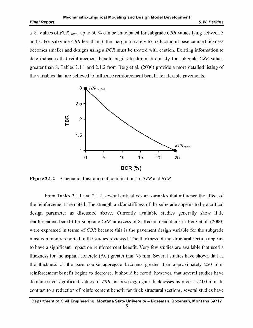
denoted by BCRTBR=1. Combinations of BCR and TBR are possible if the base course thickness is
not reduced by the full amount yielding equivalent life. A number of combinations of TBR
between 1 and TBRBCR=0 and BCR between 0 and BCRTBR=1 are possible as schematically
illustrated in Figure 2.1.2.
Based on the studies reviewed in Berg et al. (2000), values of TBRBCR=0 up to 10 can
generally be anticipated for roadways resting on a subgrade with a California bearing ratio (CBR)
Reduced σv, εv
Geosynthetic Base
course
Subgrade
Geosynthetic (+) Tensile Strain
(-)
Reduced τ
Reduced σv, εv
Reduced εh Increased σh
Mechanistic-Empirical Modeling and Design Model Development Final Report S.W. Perkins
Department of Civil Engineering, Montana State University – Bozeman, Bozeman, Montana 59717 5
# 8. Values of BCRTBR=1 up to 50 % can be anticipated for subgrade CBR values lying between 3
and 8. For subgrade CBR less than 3, the margin of safety for reduction of base course thickness
becomes smaller and designs using a BCR must be treated with caution. Existing information to
date indicates that reinforcement benefit begins to diminish quickly for subgrade CBR values
greater than 8. Tables 2.1.1 and 2.1.2 from Berg et al. (2000) provide a more detailed listing of
the variables that are believed to influence reinforcement benefit for flexible pavements.
Figure 2.1.2 Schematic illustration of combinations of TBR and BCR.
From Tables 2.1.1 and 2.1.2, several critical design variables that influence the effect of
the reinforcement are noted. The strength and/or stiffness of the subgrade appears to be a critical
design parameter as discussed above. Currently available studies generally show little
reinforcement benefit for subgrade CBR in excess of 8. Recommendations in Berg et al. (2000)
were expressed in terms of CBR because this is the pavement design variable for the subgrade
most commonly reported in the studies reviewed. The thickness of the structural section appears
to have a significant impact on reinforcement benefit. Very few studies are available that used a
thickness for the asphalt concrete (AC) greater than 75 mm. Several studies have shown that as
the thickness of the base course aggregate becomes greater than approximately 250 mm,
reinforcement benefit begins to decrease. It should be noted, however, that several studies have
demonstrated significant values of TBR for base aggregate thicknesses as great as 400 mm. In
contrast to a reduction of reinforcement benefit for thick structural sections, several studies have
1
1.5
2
2.5
3
0 5 10 15 20 25
BCR (%)
TBR
TBRBCR=0
BCRTBR=1

Mechanistic-Empirical Modeling and Design Model Development Final Report S.W. Perkins
Department of Civil Engineering, Montana State University – Bozeman, Bozeman, Montana 59717 6
demonstrated that sections that are designed for a low number of traffic passes (i.e. under
designed sections) are not appreciably influenced by base reinforcement.
Table 2.1.1 Variables influencing reinforcement effect (after Berg et al., 2000). Pavement
Component Variable Range from Test Studies/
Remarks Condition where Reinforcement Appears to Provide Most Benefit
Structure
Rigid (extruded) and flexible (knitted and woven) geogrids, woven and nonwoven geotextiles, geogrid-geotextile composites
See Table 2.1.2
Modulus (@ 2% and/or 5% strain) 100 kN/m to 750 kN/m Higher modulus improves potential
for performance
Geogrid
Moderate load (< 80 kN axle load): Bottom of thin bases (< 250 mm), middle for thick (>300 mm) bases Heavy load (> 80kN axle load): Bottom for thin bases (< 300 mm), middle for thick bases (>350mm)
Geotextile Bottom of base, on the subgrade
Location
Geogrid-geotextile composite Bottom of open-graded base OGB Surface Slick versus rough Rough
Geogrid Aperture 15 mm to 64 mm > D50 of adjacent base/subbase
Geosynthetic
Aperture Stiffness Rigid to flexible Rigid
Soil Type SP, SM, CL, CH, ML, MH, Pt No relation noted Subgrade Condition Strength CBR from 0.5 to 27
CBR # 8 (MR # 80 MPa)
Thickness 0 to 300 mm No subbase Subbase
Particle Angularity Rounded to angular Angular
Thickness 40 mm to 640 mm < 250 mm for moderate loads
Gradation Well graded to poorly graded Well graded Base
Angularity Angular to subrounded Angular
Type Asphalt, concrete, unpaved Asphalt and unpaved
Thickness 25 mm to 180 mm 75 mm Pavement
Resilient Modulus Not typically measured Unknown
Design Pavement loading 200 kPa to 1800 kPa Does not perform on significantly under-designed pavements
Construction Pre-rutting None in lab to pre-rutted in field Unknown
Mechanistic-Empirical Modeling and Design Model Development Final Report S.W. Perkins
Department of Civil Engineering, Montana State University – Bozeman, Bozeman, Montana 59717 7
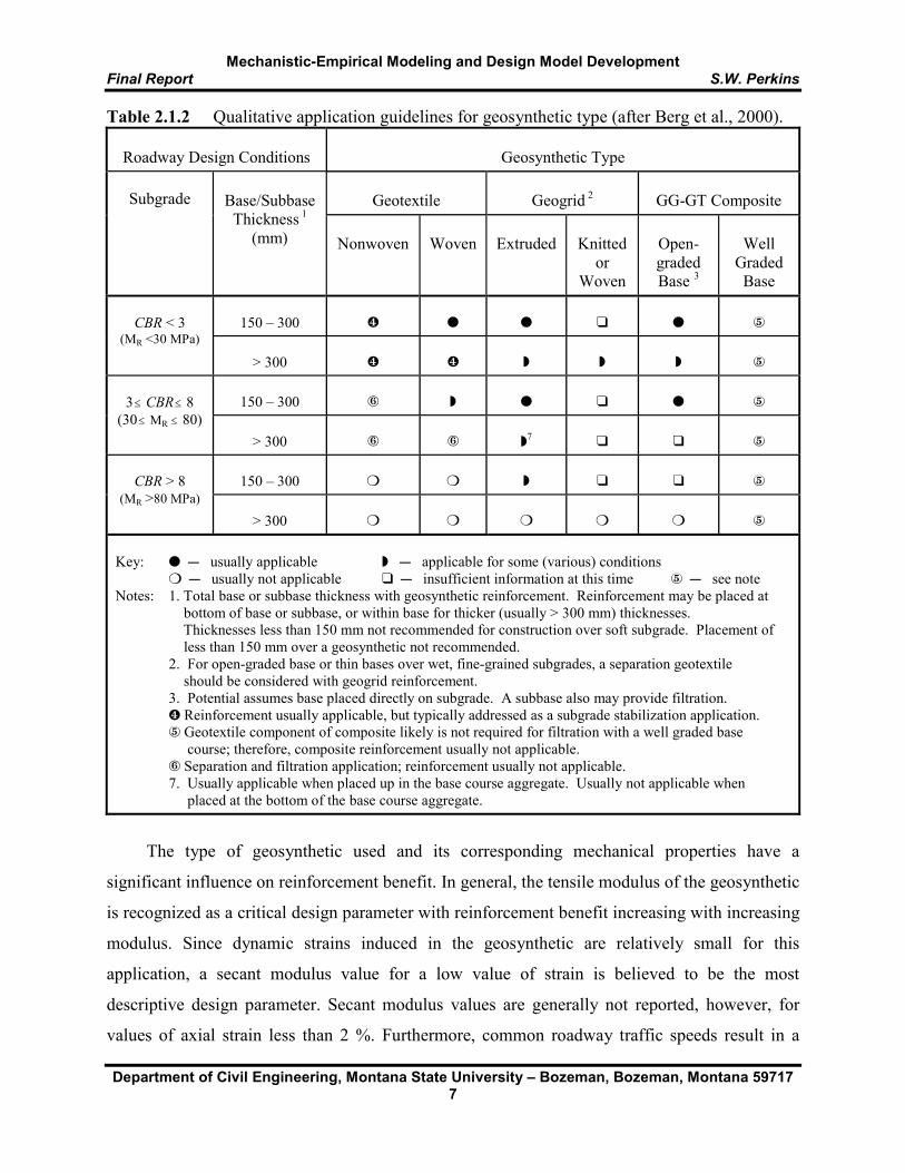
Table 2.1.2 Qualitative application guidelines for geosynthetic type (after Berg et al., 2000). Roadway Design Conditions
Geosynthetic Type
Geotextile
Geogrid 2
GG-GT Composite
Subgrade
Base/Subbase
Thickness 1 (mm)
Nonwoven
Woven
Extruded
Knitted
or Woven
Open-graded Base 3
Well
Graded Base
150 – 300
Û
�
�
“
�
Ò
CBR < 3
(MR <30 MPa) > 300
Û
Û
™
™
™
Ò
150 – 300
Ó
™
�
“
�
Ò
3# CBR# 8
(30# MR # 80) > 300
Ó
Ó
™
7
“
“
Ò
150 – 300
�
�
™
“
“
Ò
CBR > 8 (MR >80 MPa)
> 300
�
�
�
�
�
Ò Key: � C usually applicable ™ C applicable for some (various) conditions
� C usually not applicable “ C insufficient information at this time Ò C see note Notes: 1. Total base or subbase thickness with geosynthetic reinforcement. Reinforcement may be placed at
bottom of base or subbase, or within base for thicker (usually > 300 mm) thicknesses. Thicknesses less than 150 mm not recommended for construction over soft subgrade. Placement of less than 150 mm over a geosynthetic not recommended. 2. For open-graded base or thin bases over wet, fine-grained subgrades, a separation geotextile should be considered with geogrid reinforcement. 3. Potential assumes base placed directly on subgrade. A subbase also may provide filtration. Û Reinforcement usually applicable, but typically addressed as a subgrade stabilization application. Ò Geotextile component of composite likely is not required for filtration with a well graded base course; therefore, composite reinforcement usually not applicable. Ó Separation and filtration application; reinforcement usually not applicable. 7. Usually applicable when placed up in the base course aggregate. Usually not applicable when placed at the bottom of the base course aggregate.
The type of geosynthetic used and its corresponding mechanical properties have a
significant influence on reinforcement benefit. In general, the tensile modulus of the geosynthetic
is recognized as a critical design parameter with reinforcement benefit increasing with increasing
modulus. Since dynamic strains induced in the geosynthetic are relatively small for this
application, a secant modulus value for a low value of strain is believed to be the most
descriptive design parameter. Secant modulus values are generally not reported, however, for
values of axial strain less than 2 %. Furthermore, common roadway traffic speeds result in a
Mechanistic-Empirical Modeling and Design Model Development Final Report S.W. Perkins
Department of Civil Engineering, Montana State University – Bozeman, Bozeman, Montana 59717 8
loading strain rate that can be as much as 100 times greater than that employed in wide-width
tension tests, such as ASTM D 4595 (ASTM, 2001a).
Existing literature has not explicitly addressed the effect of the ratio of modulus in the
machine and cross machine directions of the geosynthetic, but it is expected that both values are
important. Since pavement loading is generally modeled as an axisymmetric loading condition
and actual roadway traffic involves loading in both directions of the material, use of the highest
modulus value would ignore the greater strains experienced in the orthogonal and less stiff
direction of the geosynthetic and the negative impact this would have on pavement performance.
The type and structure of the geosynthetic appears to influence reinforcement benefit. For
geogrids, limited data indicates that the stiffness of the aperture impacts reinforcement benefit
with increased aperture rigidity corresponding to greater benefit. The integral junctions with
rigid geogrids generally correspond to a greater potential for load transfer between the two
principal directions of the material and may offer a stiffer response under confined biaxial
loading. Limited existing literature tends to show that rigid, extruded geogrids offer greater
benefit in comparison to flexible geogrids and geotextiles, and is indicated in Table 2.1.2 by the
greater range of conditions for application of these types of geogrids. Clear distinctions between
flexible geogrids and geotextiles are not possible based on information currently available.
Geosynthetic/base aggregate interface properties may also be partly responsible for
differences in reinforcement benefit seen between geogrids and geotextiles. Geotextiles generally
rely upon surface friction for interaction while geogrids provide interaction though direct bearing
of aggregate against cross members of the mesh. Most previous studies have not reported
information from direct shear or pull out tests making it difficult to quantify differences in
interaction between different products. Complicating this, most direct shear and pull out tests are
designed to provide gross frictional properties once ultimate shearing loads have been induced.
Since this reinforcement application corresponds to a condition where shear displacements
between the geosynthetic and the aggregate are relatively small, existing interface tests may not
be capable of providing meaningful information for small shear displacements. Intuitively,
however, it should be expected that small displacement interface shear properties have an effect
on reinforcement benefit.
Mechanistic-Empirical Modeling and Design Model Development Final Report S.W. Perkins
Department of Civil Engineering, Montana State University – Bozeman, Bozeman, Montana 59717 9
2.2 Design Solutions for Geosynthetic Reinforced Pavements
Design methods proposed for geosynthetic reinforcement of flexible pavements have been based
on either empirical or analytical considerations, or analytical methods modified by experimental
data. Several studies have been summarized by Perkins and Ismeik (1997b) with others
summarized by Berg et al. (2000). Empirical methods have been typically developed for a
specific geosynthetic product or products and for a particular set of design conditions. These
methods are thereby limited by the conditions upon which they were developed. Of the few
analytical solutions that have been proposed, none have been found to address the many
variables that have been experimentally shown to impact resulting benefit.
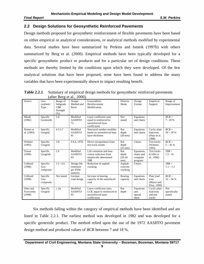
Table 2.2.1 Summary of empirical design methods for geosynthetic reinforced pavements
(after Berg et al., 2000). Source Geo-
synthetic Type
Range of Subgrade CBR Strength (%)
Design Method and Basis
Geosynthetic Reinforcement Modification
Distress Mode
Design Format
Empirical Support
Range of Improvement
Mirafi (1982)
Specific Geotextile
1-6 Modified AASHTO 72
Layer coefficient ratio equal to reinforced to unreinforced layer coefficients
Not stated
Equations and charts
BCR = 7 - 18 %
Penner et al. (1985)
Specific Geogrid
4.3-5.7 Modified AASHTO 81
Structural number modifier based on unreinforced base layer thickness
Rut depth (20 mm)
Equations and charts
Cyclic plate load tests (Haas et al. 1988)
BCR = 30 – 50 %
Webster (1993)
Specific Geogrid
3-8 FAA, 1978 Direct extrapolation from test track results
Rut depth (25 mm)
Charts Test tracks (Webster, 1993)
BCR = 5 – 45 %
Tensar (1996)
Specific Geogrids
1.9 Modified AASHTO 93
Life extension and base course reduction from empirically determined TBR
Rut depth (20-30 mm)
Equations, charts and computer program
Test tracks (Collin et al., 1996)
TBR = 1.5 - 10
Colbond (1998)
Specific Geo-composite
1.5 - 4.5 Design life extension per FEM analysis
Reduction of asphalt cracking
Asphalt concrete cracking
Charts TBR = 1.1 – 1.3
Colbond (1998)
Specific Geo-composite
Not stated German road design
Increase in bearing capacity of the unsurfaced road
Bearing capacity
Equations and charts
Plate load tests (Meyer and Elias, 1999)
BCR = 32 – 56 %
Zhao and Foxworthy (1999)
Specific Geogrid
≤ 18 Modified AASHTO 93
Layer coefficient ratio, LCR, equal to reinforced to unreinforced layer coefficients
Rut depth
Equations and spread sheet
Cyclic plate load tests and test tracks
Not specifically stated
Six methods falling within the category of empirical methods have been identified and are
listed in Table 2.2.1. The earliest method was developed in 1982 and was developed for a
specific geotextile product. The method relied upon the use of the 1972 AASHTO pavement
design method and produced values of BCR between 7 and 18 %.
Mechanistic-Empirical Modeling and Design Model Development Final Report S.W. Perkins
Department of Civil Engineering, Montana State University – Bozeman, Bozeman, Montana 59717 10
Penner et al. (1985) presented an empirical design approach stemming from the
experimental work of Haas et al. (1988). The approach used the AASHTO 1981 Interim Guide
as a basis for comparing results and developing base course equivalency charts. The structural
number (SN) of each control section was calculated assuming layer coefficients of 0.4 for the
asphalt layer and 0.14 for the granular base layer. The subgrade soil support value (S) was
determined from the CBR strength and ranged from 4.3-5.7. The values for SN and S were then
used in the AASHTO method to determine the total equivalent 80 kN single-axle load
applications, which ranged from 60,000 to 10,000,000 applications. A load correction factor was
calculated for each section by dividing the number of 80 kN single-axle load applications by the
actual number of load applications necessary to cause failure, where failure was defined as a rut
depth of 20 mm. This load correction factor was intended to account for differences in loading
conditions between the experiments and actual field moving wheel loads. For the control
sections, these ratios ranged from 3.5 to 10. The factor implies that had the laboratory section
been subjected to actual field loads, a rut depth of 20 mm would have developed after a number
of load applications equal to the number seen in the experiments multiplied by the load
correction factor.
This load correction factor was then taken to apply to the reinforced sections within a
particular test loop. The load correction factor for each reinforced section was then used to
calculate the 80 kN single-wheel load applications by multiplying the actual number of load
applications experienced in the laboratory tests by the corresponding correction factor. From the
AASHTO method, a SN for that section was determined. A structural number for the reinforced
granular base was then calculated by subtracting the asphalt layer component from the total SN.
A reinforced layer coefficient was then calculated by dividing the SN for the reinforced base by
its corresponding thickness. The ratio of the reinforced to unreinforced layer coefficients was
calculated by using the layer coefficient for the unreinforced granular base given above. For
equivalent base layer SN's, the ratio of reinforced to unreinforced layer coefficients is equal to
the ratio of unreinforced to reinforced base layer thickness. The ratio of reinforced to
unreinforced layer coefficients was plotted against the reinforced base thickness and was shown
to decrease as the reinforced base thickness approached 250 mm when the geogrid was placed at
the bottom of the base. Additional improvement in the layer coefficient ratio was noted for a
base thickness of 250 mm when the geogrid was placed in the middle of the base. Webster
Mechanistic-Empirical Modeling and Design Model Development Final Report S.W. Perkins
Department of Civil Engineering, Montana State University – Bozeman, Bozeman, Montana 59717 11
(1993) produced a design chart similar to that of Haas et al. (1988) by direct comparison and
extrapolation of test results for sections of equivalent base course thickness.
The method proposed by Tensar (1996) is based on the test section work performed by
Collin et al. (1996). The method relies on the identification of TBR for the application. Charts are
given defining TBR as a function of base course thickness for three levels of rut depth (20, 25
and 30 mm). The values of TBR listed in these charts were generated from the test section work
of Collin et al. (1996) and pertain to a subgrade with an average CBR of 1.9. With the definition
of TBR, a life-cycle analysis could be performed by extending the life of the roadway or the
AASTHO ’93 guide could be used to calculate a BCR value. Test sections were not conducted to
verify BCR values determined through this method.
Colbond (1998) developed a method that fits within the framework of the German practice
for roadway design. This practice relies upon achieving a particular bearing capacity of the base-
subgrade system prior to proceeding with the placement of surfacing material. Plate load tests are
typically conducted to evaluate the modulus of the system. Tests reported by Meyer and Elias
(1999) serve as empirical support for the method.
Zhao and Foxworthy (1999) also used the AASHTO design method to determine a layer
coefficient ratio for the granular base, which equaled the ratio of the reinforced to unreinforced
layer coefficients. Values of this ratio were determined from experiments using one geogrid and
subgrades with different CBR strengths and ranged from 2 to 1.5, with values greater than 1.5
being obtained for CBR strengths less than 3. This ratio was used as a multiplication factor on
the depth of the reinforced base inside the equation for structural number, implying that for an
equivalent structural number, the unreinforced base could be reduced by 33 to 50 %.
Three methods falling within the category of methods based on analytical considerations
have been identified. Davies and Bridle (1990) developed an analytical technique to determine
the development of permanent deformation (rut depth) with load cycle of reinforced pavements.
The displacement response of the pavement under a single monotonic load application was
predicted using an energy method. An expression for the potential energy of the pavement
system was developed as a function of the central displacement of the applied load. The general
shape of the surface displacement profile was assumed to match that seen in previously
published studies. The geosynthetic layer provided an additional energy component to the
system as it deformed and was shown to increase the component of strain energy provided by the

Mechanistic-Empirical Modeling and Design Model Development Final Report S.W. Perkins
Department of Civil Engineering, Montana State University – Bozeman, Bozeman, Montana 59717 12
base layer of the pavement. Both the base layer and the geosynthetic were assumed to provide a
component of strain energy as they functioned as a structural member in bending, even though
both materials have little flexural rigidity.
The development of permanent deformation with increasing load cycle was predicted by
varying the stiffness parameters of the subgrade. Permanent deformation was assumed to be
negligible in the base layer. The stiffness parameters of the subgrade during loading were
assumed to be less than those during unloading. Each set of stiffness parameters were assumed
to vary with increasing load cycle, with the difference between the two sets becoming less at an
ever decreasing rate. The net effect of this type of material model was a prediction of rut depth
that increased with load cycle at a decreasing rate. The values and variation of these parameters
were determined primarily from the results of repeated load experiments on reinforced pavement
test sections. In this way, the material parameters were empirically derived from the tests for
which the parameters are being used to predict. Use of this technique will require that these
parameters be related to material properties, such as resilient modulus, that can be more readily
determined from element tests.
Sellmeijer (1990) formulated a model for the behavior of a soil-geotextile-aggregate system
that accounted for both the membrane action and lateral restraint function of the geotextile.
While an AC layer was not specifically included in the model, the model was said to be suitable
for paved roads owing to its ability to analyze situations where only small rut depths were
permissible. The model used an elastic-plastic model for the aggregate. The subgrade was taken
as a rigid-perfectly plastic material. Interaction between the soil and geotextile was accounted
for using a simple law of friction. The function of lateral restraint was shown to increase the
mean stress and stiffness in the aggregate layer. The model was not compared to experimental
results.
Colbond (1998) has presented a method based in part on the work of Liu et al. (1998). The
method involves the examination of crack initiation and propagation in the asphalt concrete for
reinforced base layers through a finite element study. The number of load cycles necessary to
create asphalt fatigue was examined, with life increasing by 10 to 30 % with the addition of
reinforcement (i.e. TBR = 1.1 to 1.3). This work was not compared to results from experimental
test sections.

Mechanistic-Empirical Modeling and Design Model Development Final Report S.W. Perkins
Department of Civil Engineering, Montana State University – Bozeman, Bozeman, Montana 59717 13
2.3 Summary of an Existing Recommended Standard of Practice
The document developed by the GMA for the AASHTO Subcommittee on Materials Technical
Section 4E (Berg et al., 2000) contained a recommended standard of practice (SOP) based on the
research and case histories reviewed for the report. This SOP has now been adopted by the
AASHTO Subcommittee and is contained in the AASHTO Designation PP 46-01 (AASHTO
2001). The purpose of this section is to summarize the recommended standard of practice given
by Berg et al. (2000) for the purpose of identifying how research described in this report can be
used within the SOP.
The recommended SOP given in Berg et al. (2000) relies upon the assessment of
reinforcement benefit as defined by a Traffic Benefit Ratio (TBR), a Base Course reduction Ratio
(BCR) or a combination of the two. Reinforcement benefit defined in terms of TBR and BCR is
then used to modify an existing unreinforced pavement design.
The steps involved in the recommended SOP consist of:
Step 1. Initial assessment of applicability of the technology.
Step 2. Design of the unreinforced pavement.
Step 3. Definition of the qualitative benefits of reinforcement for the project.
Step 4. Definition of the quantitative benefits of reinforcement (TBR and/or BCR).
Step 5. Design of the reinforced pavement using the benefits defined in Step 4.
Step 6. Analysis of life-cycle costs.
Step 7. Development of a project specification.
Step 8. Development of construction drawings and bid documents.
Step 9. Construction of the roadway.
Step 1 involves assessing the project related variables described in Tables 2.1.1 and 2.1.2
and making a judgment on whether the project conditions are favorable or unfavorable for
reinforcement to be effective and what types of reinforcement products (as defined in Table
2.1.2) are appropriate for the project. Step 2 involves the design of a conventional unreinforced
typical pavement design cross-section or a series of cross sections, if appropriate, for the project.
Any acceptable design procedure can be used for this step. Step 3 involves an assessment of the
qualitative benefits that will be derived by the addition of the reinforcement. The two main
benefits that should be assessed are whether the geosynthetic will be used for an extension of the
life of the pavement (i.e. the application of additional vehicle passes), a reduction of the base

Mechanistic-Empirical Modeling and Design Model Development Final Report S.W. Perkins
Department of Civil Engineering, Montana State University – Bozeman, Bozeman, Montana 59717 14
aggregate thickness or a combination of the two. Berg et al. (2000) has listed additional
secondary benefits that should also be considered.
Step 4 requires the definition of the value, or values, of benefit (TBR and/or BCR) that will
be used in the design of the reinforced pavement. In the absence of a suitable solution for the
definition of these values, Berg et al. (2000) suggested that these values be determined through
empirical means by a careful comparison of project design conditions, as defined in previous
steps, to conditions present in studies reported in the literature. In the absence of suitable
comparison studies, an experimental demonstration method involving the construction of
reinforced and unreinforced pavement test sections has been suggested and described in Berg et
al. (2000) and may be used for the definition of benefit for the project conditions. The research
described in this report is designed to provide for a quantitative solution for values of benefit
defined in terms of TBR and/or BCR.
Step 5 involves the direct application of TBR or BCR to modify the unreinforced pavement
design defined in Step 2. TBR can be directly used to define an increased number of vehicle
passes that can be applied to the pavement while BCR can be used to define a reduced base
aggregate thickness such that equal life results. If combinations of TBR and BCR are provided,
each can be used according to the usage described above for a combined effect.
With the unreinforced and reinforced pavement designs defined, a life-cycle cost analysis
should be performed to assess the economic benefit of reinforcement. This step will dictate
whether it is economically beneficial to use the geosynthetic reinforcement. Remaining steps
involve the development of project specifications, construction drawings, bid documents and
plans for construction monitoring. Berg et al. (2000) has presented a draft specification that may
be adopted for this application.
The research described in this report provides a quantitative and general means of
identifying values of benefit defined in terms of TBR and/or BCR needed for Step 4 of the
recommended SOP. The design model developed for the definition of TBR and/or BCR values is
general in the sense that it can be used to assess benefit values for a wide range of pavement
design conditions and reinforcement products.

Mechanistic-Empirical Modeling and Design Model Development Final Report S.W. Perkins
Department of Civil Engineering, Montana State University – Bozeman, Bozeman, Montana 59717 15
21
kR kM θ=
2.4 Mechanistic-Empirical Modeling of Flexible Pavements
Mechanistic-empirical modeling of flexible pavements relies upon the use of a numerical model
to describe the response of the pavement system to an externally applied load representative of
the traffic to which the roadway will be subjected. The response extracted from the model is
typically a measure of stress, strain or deflection for one or several critical points within the
pavement system. Several types of numerical or response models are available for pavement
analysis and design. Multi-layered elastic (MLE) programs, such as DAMA (Asphalt Institute,
1991), ELSYM5 (Kopperman et al., 1986) and KENLAYER (Huang, 1993) rely upon the
solution of differential equations for layered elastic systems. Finite element (FE) models, such as
ILLI-PAVE (1990) and MICH-PAVE (Harichandran et al., 1989) typically consist of two-
dimensional axi-symmetric models.
Response models typically use elastic material models for the asphalt concrete (AC), base
aggregate and subgrade layers. These material models may be linear or non-linear and may be
isotropic or anisotropic. Models using nonlinear elastic material models generally express the
elastic modulus, or resilient modulus, as a function of stress state, whereas linear elastic models
treat the elastic modulus of the materials as a constant for all stress states. A common non-linear
elastic model for relating the resilient modulus of aggregates to stress state is given by Equation
2.4.1 (Seed et al., 1967), where MR is resilient modulus, θ is the bulk stress defined as the sum of
the three principal stresses and k1 and k2 are material constants. Chen et al. (1995) has provided a
summary of response models commonly used for pavement modeling. (Refer to Appendix A for
a listing of all notation used in this report).
(2.4.1)
The response measures extracted from response models are typically related to long-term
pavement performance through empirically derived damage models. The two most common
types of damage models are those that relate the tensile strain in the bottom of the asphalt to
asphalt fatigue life and ones that use the vertical compressive strain in the top of the subgrade to
control permanent deformation of the pavement structure. The later was introduced by Dorman
and Metcalf (1965) and was later expressed in the form of Equation 2.4.2, where N is the number

Mechanistic-Empirical Modeling and Design Model Development Final Report S.W. Perkins
Department of Civil Engineering, Montana State University – Bozeman, Bozeman, Montana 59717 16
BvAN −= ε
of load cycles necessary to reach a certain permanent deformation of the pavement surface, εv is
the vertical strain in the top of the subgrade and A and B are constants.
(2.4.2)
2.5 Modeling of Geosynthetic Reinforced Pavements
A number of studies have been conducted to examine the utility of finite element programs to
predict the response of roadways reinforced with geosynthetics. Several of these studies have
been performed in conjunction with experimental studies such that comparisons between model
predictions and experimental results could be made. For the studies discussed below, Table 2.3.1
has been created to summarize the major features associated with each study’s model.
Barksdale et al. (1989) adapted an existing finite element model to predict the response
seen in the experimental portion of their study. The prediction of tensile strain in the base
material was essential in determining the level of tensile strain developed in the geosynthetic,
which in turn determined, in part, the benefit provided by the reinforcement. The cross-
anisotropic linear elastic model used for the base was the only model capable of simultaneously
predicting the lateral tensile strains in the bottom of the base and the small vertical strains in the
bottom and upper part of that layer, as observed in the laboratory experiments.
The finite element model was calibrated and verified by using data from an unreinforced
pavement section from a previous study and from the test data generated from one of the
experimental test series of their study. The unreinforced pavement section used for calibration
was strong in comparison to the sections described for their study. The finite element model was
capable of predicting measured variables to within +/- 20 % for the strong unreinforced section.
For the weaker sections used in the study described as part of their work, the finite element
predictions were not as good. The strain in the geosynthetic was over predicted by about 33 %
when the geosynthetic was located in the bottom of the base. It was under predicted by about 14
% when located in the middle of the layer. The vertical stress and vertical strain on the top of the
subgrade was under predicted by about 50 %. The lateral strains were also under predicted by
about 50 %.

Mechanistic-Empirical Modeling and Design Model Development Final Report S.W. Perkins
Department of Civil Engineering, Montana State University – Bozeman, Bozeman, Montana 59717 17
Table 2.5.1 Summary of Finite Element Studies of Geosynthetic Reinforced Pavements.
Author Barksdale et al. (1989) Burd & Houlsby (1986) Burd & Brocklehurst
(1990) Burd & Brocklehurst
(1992) Dondi (1994) Miura et al. (1990) Wathugala et al.
(1996) Analysis Type Axi-symmetric Plane strain Plane strain Plane strain Three-dimensional Axi-symmetric Axi-symmetric
AC Constitutive
Model
Isotropic, non-linear elastic
None None None Isotropic, linear elastic
Isotropic, linear elastic
Isotropic elastoplastic, D-P
AC Thickness (mm)
Variable None None None 120 50 89
Base Constitutive
Model
Anisotropic, linear elastic
Isotropic, elastoplastic, Matusoka
Isotropic, elastoplastic, Matusoka
Isotropic, elastoplastic, Matusoka
Isotropic, elastoplastic, D-P
Isotropic, linear elastic
Isotropic, elastoplastic, D-P
Base Thickness
(mm)
Variable 75 300 300 300 150 140
Geosynthetic Constitutive
Model
Isotropic, linear elastic Isotropic, linear elastic Isotropic, linear elastic Isotropic, linear elastic Isotropic, linear elastic
Isotropic, linear elastic
Isotropic, elastoplastic, von
Mises Geosynthetic Element Type
Membrane Membrane Membrane Membrane Membrane Truss Solid continuum
Geosynthetic Thickness
(mm)
None None None None None None 2
Interface Elements &
Model
Linear elastic- perfectly plastic
None None Elastoplastic, Mohr-Coulomb
Elastoplastic, Mohr-Coulomb
Linear elastic joint element
None
Subbase Constitutive
Model
None None None None None Isotropic, linear elastic
Isotropic, elastoplastic,HiSS
δo Subbase
Thickness (mm)
None None None None None 200 165
Subgrade Constitutive
Model
Isotropic, non-linear elastic
Isotropic, elastoplastic, von Mises
Isotropic, elastoplastic, von Mises
Isotropic, elastoplastic, von Mises
Isotropic, elastoplastic, Cam-
Clay
Isotropic, linear elastic
Isotropic, elastoplastic, HiSS
δo Load
Application Monotonic Monotonic, footing width
= 75 mm Monotonic, footing width
= 500 mm Monotonic, footing
width = 500 mm Monotonic, two
rectangular areas, 240 mm x 180 mm
Monotonic, 200 mm diameter plate
Single cycle, peak pressure = 725 kPa
on a 180 mm diameter plate
Remarks on Observed
Improvement
Base layer could be reduced in thickness by 4-18 %. Greater
improvement seen for sections with weak
subgrade
Improvement seen after a penetration of 4 mm. Model over predicted
improvement beyond a 4 mm displacement
Improvement seen after a penetration of 12 mm. Improvement increased
with increasing geosynthetic stiffness.
Improvement seen after a penetration of
25 mm.
15-20 % reduction in vertical displacement, fatigue life of section increased by a factor
of 2-2.5
5 % reduction in vertical displacement.
Improvement level did not match
experimental results.
20 % Reduction in Permanent
Displacement
D-P: Drucker-Prager
Mechanistic-Empirical Modeling and Design Model Development Final Report S.W. Perkins
Department of Civil Engineering, Montana State University – Bozeman, Bozeman, Montana 59717 18
A parametric study was conducted with the finite element model to calculate the lateral
tensile strain at the bottom of the AC layer and the vertical strain at the top of the subgrade for a
single load application. This was used for evaluations of fatigue resistance and to indicate the
degree of rutting that would occur, which in turn was used to evaluate the improvement in
pavement performance when reinforcement was added. Reinforcement improvement was
quantified as the reduction in aggregate base thickness for a reinforced roadway giving the same
tensile strain (fatigue) and vertical strain (reflecting permanent deformation) as that for the
unreinforced section. Improvement was seen to increase with increasing geosynthetic stiffness,
and to decrease with increasing subgrade stiffness and asphalt thickness. Optimal improvement
was seen when the geosynthetic was placed between the bottom of the base and 1/3 up into the
base layer.
Barksdale et al. (1989) used the 1972 AASHTO design method to determine design
thickness for the sections with subgrade CBR strengths ranging from 3 to 10 and for two
different traffic loading conditions. Using the more stiff geosynthetic, reductions in base course
thickness ranged between 4 to 16 % when improvement was based on equal lateral strain in the
bottom of the AC layer and 6 to 18 % when improvement was based on equal vertical strain at
the top of the subgrade. In general, more improvement was observed for sections with a weak
subgrade and a thinner AC layer. The magnitude of benefit defined in this study is less than
those for a preponderance of experimental studies as summarized by Berg et al. (2000).
Barksdale et al. (1989) felt that the mechanisms modeled were more suited for geotextiles and
that additional research was needed to define the mechanisms of improvement associated with
geogrids and to develop suitable models.
Burd and Houlsby (1986) developed a large strain finite element model for the purpose of
examining the experimental results of reinforced unpaved roads, but could be extended to
include material elements representing an asphalt layer. The large strain formulation was
included to account for the extensive rutting that can take place in unpaved roads. Interface
elements were not included in the formulation, which implies perfect fixidity between the soil
layers and the geosynthetic. The model was used to predict the response of a footing resting on a
base layer with a geosynthetic layer placed between the base and the underlying subgrade. The
model predictions were compared to experimental results and shown to match reasonably well.
The experimental results showed a slight improvement in the load-displacement curve for the
Mechanistic-Empirical Modeling and Design Model Development Final Report S.W. Perkins
Department of Civil Engineering, Montana State University – Bozeman, Bozeman, Montana 59717 19
reinforced footing for footing penetrations less than 4 mm, while the model did not show
improvements of this kind until the footing penetration exceeded 4 mm. Beyond a penetration of
4 mm, the improvement exhibited by the reinforced footing became significant for both the
model and the experimental results, with the model over predicting the experimental results at
larger displacements and with this over prediction becoming more significant as the footing
displacement increased.
Burd and Brocklehurst (1990) applied this same model to a larger footing. Similar to the
results of Burd and Houlsby (1986) the model did not show improvements in the load-
displacement curve until a settlement of 12 mm was reached. The model was used in a
parametric study to demonstrate the importance of the geosynthetic stiffness on improvement
levels.
Burd and Brocklehurst (1992) extended this model to include interface elements. The
model was used to predict the response of a footing placed on a base material over top of a
subgrade with reinforcement between the base and subgrade. The finite element analyses
predicted negligible improvement in the load versus displacement response until a displacement
of over 25 mm was reached. In general, the model with interface elements tended to show less
improvement than the earlier version without these elements. In light of the results of Burd and
Houlsby (1986), where model results were compared to experimental results, it appears that
interface elements were needed only when large footing displacements were present.
Dondi (1994) used the commercial code ABAQUS to model a geosynthetic reinforced
pavement. Load was applied to the pavement surface by two rectangular areas measuring 240
mm by 180 mm and representing a single pair of dual wheels. A distance of 120 mm separated
the wheels. Each rectangular area experienced a peak loading pressure of 1500 kPa. Due to the
loading geometry, a three-dimensional finite element analysis was performed. A cohesion of 60
kPa was assigned to the base course soil to avoid numerical instabilities. Different friction
coefficients were used between the geosynthetic and the base and subgrade soils. Sections were
analyzed with and without the geosynthetic layer and for two geosynthetics of differing elastic
modulus.
The evaluation of stress and strain measures for elements in the base and in the subgrade
indicated that the base layer experienced moderate increases in load carrying capacity for the
reinforced cases while the strain in the subgrade was seen to decrease substantially for the

Mechanistic-Empirical Modeling and Design Model Development Final Report S.W. Perkins
Department of Civil Engineering, Montana State University – Bozeman, Bozeman, Montana 59717 20
reinforced cases. The model indicated that the geosynthetic layer reduced the shear stresses and
strains experienced by the subgrade. Vertical displacement of the loaded area was reduced by 15
to 20 % by the inclusion of the geosynthetic. The displacement of the unreinforced section was
not indicated. An empirical power expression involving tensile strain in the AC layer was used
to evaluate the fatigue life of the sections, showing that the life of the reinforced sections could
be increased by a factor of 2 to 2.5 as compared to the unreinforced section.
Miura et al. (1990) performed a finite element analysis of a reinforced paved road in
support of a laboratory and field experimental program. The section layer thicknesses were
chosen to match the laboratory test sections. The results from the analysis of reinforced and
unreinforced sections showed general agreement with results from the laboratory test sections
where surface displacement and strain in the geosynthetic were plotted against distance from the
centerline of the load. The improvement in the surface displacement for the reinforced section as
compared to the unreinforced section was greatly underestimated by the finite element model as
compared to the experimental results. The finite element model showed a reduction in
displacement of 5 % while the experiment showed a 35 % reduction. The monotonic loading
results from the finite element analysis were compared to the experimental results at 10,000
cycles of applied load. In this light, the finite element model was not intended to be an exact
representation of the experiments but were intended more to shed light on the mechanisms
involved in reinforcement.
Wathugala et al. (1996) used the commercial program ABAQUS to formulate a finite
element model of a geogrid reinforced pavement. The base aggregate and subgrade soils were
modeled using the hierarchical constitutive model developed by Desai et al. (1986) and
Wathugala and Desai (1993). This model can account for non-linear behavior during non-virgin
loading, which is particularly appropriate for cyclic loading applications. This feature was not
used, however, with non-virgin loading modeled by a linear elastic response. No special
interface models were used between the geogrid and the surrounding soil. The geosynthetic was
given a thickness of 2.5 mm. The pavement section was analyzed with and without the geogrid
layer. The addition of the geogrid was shown to reduce the permanent rut depth by
approximately 20 % for a single cycle of load. This level of improvement was most likely due
the flexural rigidity of the geosynthetic, which is an artificial feature arising from the material
and element model used for the geosynthetic.
Mechanistic-Empirical Modeling and Design Model Development Final Report S.W. Perkins
Department of Civil Engineering, Montana State University – Bozeman, Bozeman, Montana 59717 21
asm
aT
Gε
ε=
2.6 Tension and Interface Testing of Geosynthetics
Tensile properties of geosynthetics are most commonly determined through the use of wide-
width tension tests, ASTM D 4595 (ASTM, 2001a). This test standard is currently developed for
geotextiles while a draft standard exists for geogrids. Properties reported from these tests
typically consist of ultimate strength and strength at 2 %, 5 % and perhaps at higher values of
axial strain. Strength at various levels of axial strain can be used to determine a secant tensile
modulus for that level of axial strain according to Equation 2.6.1, where GSM is the geosynthetic
secant tensile modulus, Tεa is the tensile strength at a certain level of axial strain and εa is the
value of axial strain for which the modulus is determined and is in decimal form. It is not
common for values of strength at axial strain levels less than 2 % to be reported. Since strength
values for geosynthetics are often times different in the two principal directions of the material, it
is common to perform tests in each of the two material directions (machine and cross-machine
directions) and report values for each.
(2.6.1)
Interface testing of geosynthetics and soil (or base aggregate) is commonly performed by
conducting direct shear tests, ASTM D 5321 (ASTM, 2001a), and pull out tests, GRI GT6 or
GG5 (GRI, 2001). Coefficients of interaction are typically computed for ultimate values of
shearing resistance generally corresponding to large levels of displacement. Test protocols have
not been developed for the accurate determination of small displacement shear resistance, as may
be a more appropriate measure of interaction for base reinforcement applications.
3.0 PRIOR TEST SECTION WORK
Previous work supported by the Montana Department of Transportation focused on the
construction and evaluation of geosynthetic reinforced pavement test sections constructed in a
facility located at Montana State University (MSU). Test sections were constructed for the
purpose of providing data to evaluate the mechanisms by which geosynthetics serve to reinforce
flexible pavements and to provide data to which the models, developed as part of this work,
could be compared. Perkins (1999a,b) provides detailed information describing the pavement test
facility, the construction process, instrumentation used and results obtained. Other papers related
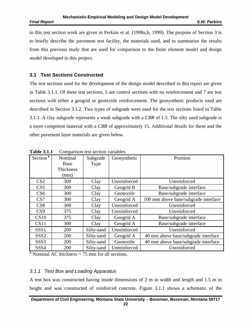
Mechanistic-Empirical Modeling and Design Model Development Final Report S.W. Perkins
Department of Civil Engineering, Montana State University – Bozeman, Bozeman, Montana 59717 22
to this test section work are given in Perkins et al. (1998a,b, 1999). The purpose of Section 3 is
to briefly describe the pavement test facility, the materials used, and to summarize the results
from this previous study that are used for comparison to the finite element model and design
model developed in this project.
3.1 Test Sections Constructed
The test sections used for the development of the design model described in this report are given
in Table 3.1.1. Of these test sections, 5 are control sections with no reinforcement and 7 are test
sections with either a geogrid or geotextile reinforcement. The geosynthetic products used are
described in Section 3.1.2. Two types of subgrade were used for the test sections listed in Table
3.1.1. A clay subgrade represents a weak subgrade with a CBR of 1.5. The silty sand subgrade is
a more competent material with a CBR of approximately 15. Additional details for these and the
other pavement layer materials are given below.
Table 3.1.1 Comparison test section variables. Section a Nominal
Base Thickness
(mm)
Subgrade Type
Geosynthetic Position
CS2 300 Clay Unreinforced Unreinforced CS5 300 Clay Geogrid B Base/subgrade interface CS6 300 Clay Geotextile Base/subgrade interface CS7 300 Clay Geogrid A 100 mm above base/subgrade interface CS8 300 Clay Unreinforced Unreinforced CS9 375 Clay Unreinforced Unreinforced
CS10 375 Clay Geogrid A Base/subgrade interface CS11 300 Clay Geogrid A Base/subgrade interface SSS1 200 Silty-sand Unreinforced Unreinforced SSS2 200 Silty-sand Geogrid A 40 mm above base/subgrade interface SSS3 200 Silty-sand Geotextile 40 mm above base/subgrade interface SSS4 200 Silty-sand Unreinforced Unreinforced
a Nominal AC thickness = 75 mm for all sections. 3.1.1 Test Box and Loading Apparatus
A test box was constructed having inside dimensions of 2 m in width and length and 1.5 m in
height and was constructed of reinforced concrete. Figure 3.1.1 shows a schematic of the

Mechanistic-Empirical Modeling and Design Model Development Final Report S.W. Perkins
Department of Civil Engineering, Montana State University – Bozeman, Bozeman, Montana 59717 23
pavement test facility. A load frame was constructed to rest and ride on I-beams set into the
concrete walls. A load actuator, consisting of a pneumatic cylinder with a 305 mm diameter bore
and a stroke of 75 mm, is used to apply a cyclic load to the pavement. A 50 mm diameter steel
rod 300 mm in length extends from the piston of the actuator. The rod is rounded at its tip and
fits into a cup welded on top of the load plate that rests on the pavement surface.
Figure 3.1.1 Schematic diagram of the pavement test facility.
The load plate consists of a 305 mm diameter steel plate with a thickness of 25 mm. A 4
mm thick, waffled butyl-rubber pad was placed beneath the load plate in order to provide a
uniform pressure and avoid stress concentrations along the plate’s perimeter.
A binary solenoid regulator attached to a computer controlled the load-time history applied
to the plate. The software controlling the load pulse was set up to provide the load or plate
pressure pulse shown in Figure 3.1.2. This pulse has a linear load increase from zero to 40 kN
over a 0.3 second rise time, followed by a 0.2 second period where the load is held constant,
followed by a load decrease to zero over a 0.3 second period and finally followed by a 0.7
second period of zero load before the load cycle is repeated, resulting in a load pulse frequency
of 0.67 Hz.
2 m
Rollers
Geosynthetic Subgrade
Base
AC
1.50 m
Load actuator
φ 305 mm Load cell Surface LVDT
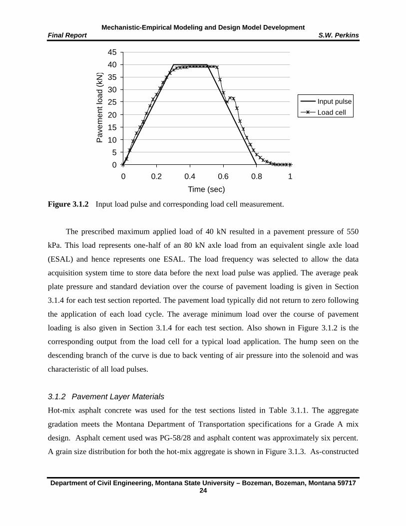
Mechanistic-Empirical Modeling and Design Model Development Final Report S.W. Perkins
Department of Civil Engineering, Montana State University – Bozeman, Bozeman, Montana 59717 24
Figure 3.1.2 Input load pulse and corresponding load cell measurement.
The prescribed maximum applied load of 40 kN resulted in a pavement pressure of 550
kPa. This load represents one-half of an 80 kN axle load from an equivalent single axle load
(ESAL) and hence represents one ESAL. The load frequency was selected to allow the data
acquisition system time to store data before the next load pulse was applied. The average peak
plate pressure and standard deviation over the course of pavement loading is given in Section
3.1.4 for each test section reported. The pavement load typically did not return to zero following
the application of each load cycle. The average minimum load over the course of pavement
loading is also given in Section 3.1.4 for each test section. Also shown in Figure 3.1.2 is the
corresponding output from the load cell for a typical load application. The hump seen on the
descending branch of the curve is due to back venting of air pressure into the solenoid and was
characteristic of all load pulses.
3.1.2 Pavement Layer Materials
Hot-mix asphalt concrete was used for the test sections listed in Table 3.1.1. The aggregate
gradation meets the Montana Department of Transportation specifications for a Grade A mix
design. Asphalt cement used was PG-58/28 and asphalt content was approximately six percent.
A grain size distribution for both the hot-mix aggregate is shown in Figure 3.1.3. As-constructed
0
5
10
15
20
25
30
35
40
45
0 0.2 0.4 0.6 0.8 1
Time (sec)
Pav
emen
t loa
d (k
N)
Input pulse
Load cell

Mechanistic-Empirical Modeling and Design Model Development Final Report S.W. Perkins
Department of Civil Engineering, Montana State University – Bozeman, Bozeman, Montana 59717 25
properties of the AC for each test section are given in Section 3.1.4. Results from indirect tension
resilient modulus tests are presented in Section 4.1.
Figure 3.1.3 Grain size distribution of AC and base aggregate and silty sand subgrade.
The geosynthetics used for the test sections shown in Table 3.1.1 are listed with their
properties as reported by the manufacturers in Table 3.1.2.
A crushed-stone base course was used for all experimental test sections. The base course
grain size distribution is shown in Figure 3.1.3, where it is seen that 100 % passes the 19 mm
sieve. The material is classified as an A-1-a or a GW. Specific gravity of the material is 2.63.
Modified Proctor tests resulted in a maximum dry unit weight of 21.5 kN/m3 at an optimum
moisture content of 7.2 %. This material was typically compacted at a moisture content of 6.3 %
and to a dry unit weight of 21 kN/m3. As-constructed properties of the base course for each test
section are given in Section 3.1.4. A series of triaxial tests were performed on this material and
are presented in Section 4.2 when the constitutive model for this material is described and
calibrated. The triaxial tests yielded a drained friction angle of approximately 48 degrees.
To provide information on the influence of subgrade strength on reinforcement benefits,
two subgrade materials were used in this study. A highly plastic clay subgrade was used to
represent a soft subgrade while a silty-sand was used to represent a hard subgrade. The soft
subgrade consisted of a CH or A7-(6) clay, having a liquid limit of 100 % and a plastic limit of
0102030405060708090
100
0.0010.010.1110100
Particle size (mm)
Per
cent
pas
sing
(%)
Cold-mix asphalt
Hot-mix asphalt
Basecourse
Silty-Sand Subgrade
0
10
20
30
40
50
60
70
80
90
100
0.001 0.01 0.1 1 10 100
Particle size (mm)
Hot-mix asphalt aggregate
Basecourse
Silty-Sand Subgrade

Mechanistic-Empirical Modeling and Design Model Development Final Report S.W. Perkins
Department of Civil Engineering, Montana State University – Bozeman, Bozeman, Montana 59717 26
40 %. One hundred percent of the clay material passes the #200 sieve. Specific gravity of the
clay is 2.70. Modified Proctor compaction tests resulted in a maximum dry density of 16.0
kN/m3 occurring at an optimum moisture content of 20.0 %. The clay was compacted at a
moisture content of approximately 45 % in order to obtain a CBR of 1.5.
Table 3.1.2 Geosynthetic material properties. Geogrid A:
Tensar BX-1100 Geogrid B:
Tensar BX-1200 Geotextile:
Amoco 2006 Material Polypropylene Polypropylene Polypropylene Structure Punched
Drawn, Biaxial Punched
Drawn, Biaxial Woven
Mass/Unit Area (g/m2) 2151 3091 2503
Aperature Size (mm) Machine Direction Cross-Machine Direction
251 331
251 331
None
Wide-Width Tensile Strength at 2 % Strain (kN/m) Machine Direction Cross-Machine Direction
5.062 8.52
7.322 11.92
4.254 13.64
Wide-Width Tensile Strength at 5 % Strain (kN/m) Machine Direction Cross-Machine Direction
9.712 16.51
13.42 22.92
11.94 26.44
Ultimate Wide-Width Tensile Strength (kN/m) Machine Direction Cross-Machine Direction
13.82 21.22
21.12 31.32
40.24 42.94
1 IFAI, 1994; 2 Tensar, 2001; 3 AMOCO, 1996; 4 AMOCO, 2001
The target moisture content of 45 % was established by conducting laboratory, unsoaked
CBR tests. Figure 3.1.4 shows the variation of CBR with compaction moisture content. On this
figure, it is noted that only a relatively small change in CBR results between a moisture content
range of 43 to 46 %.
The hard subgrade (approximate CBR=15 at a moisture content of 14 %) consisted of fines
trapped from the baghouse of a local batch hot-mix plant. The material is classified as a SM or
A-4, with 40 % non-plastic fines and a liquid limit of 18 %. Specific gravity of the silty-sand is
2.68. Modified Proctor tests resulted in a maximum dry density of 18.2 kN/m3 occurring at a

Mechanistic-Empirical Modeling and Design Model Development Final Report S.W. Perkins
Department of Civil Engineering, Montana State University – Bozeman, Bozeman, Montana 59717 27
moisture content of 11.5 %. This material was typically compacted at a moisture content of 14.8
% and a dry unit weight of 17.5 kN/m3.
Figure 3.1.4 CBR versus compaction moisture content for the clay subgrade.
As constructed properties of the compacted clay and silty sand subgrade in the test sections
are given in Section 3.1.4. Shelby tubes were pushed into the subgrade during excavation of the
sections for each test section. Undisturbed samples were used to conduct triaxial tests, with
results presented in Section 4.2 where the constitutive model for the subgrade materials is
presented and calibrated.
3.1.3 Instrumentation
An extensive array of instrumentation was used in the test sections to quantify the mechanical
response of the pavement materials to pavement loading. This data has allowed for the
description of reinforcement mechanisms and has provided data to which the models developed
in this report have been compared. The test sections contained instruments to measure applied
pavement load, surface deflection, and stress and strain in the various pavement layers.
Instrumentation has been categorized into sensors measuring applied pavement load, asphalt
surface deflection, stress and strain in the base course and subgrade, and strain on the
geosynthetic. Data acquisition software was configured to record information on the full time-
history of response for prescribed load cycles and maximum and minimum sensor response for
0
1
2
3
4
5
6
36 37 38 39 40 41 42 43 44 45 46 47 48
Water content, %
CB
R
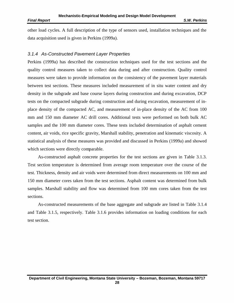
Mechanistic-Empirical Modeling and Design Model Development Final Report S.W. Perkins
Department of Civil Engineering, Montana State University – Bozeman, Bozeman, Montana 59717 28
other load cycles. A full description of the type of sensors used, installation techniques and the
data acquisition used is given in Perkins (1999a).
3.1.4 As-Constructed Pavement Layer Properties
Perkins (1999a) has described the construction techniques used for the test sections and the
quality control measures taken to collect data during and after construction. Quality control
measures were taken to provide information on the consistency of the pavement layer materials
between test sections. These measures included measurement of in situ water content and dry
density in the subgrade and base course layers during construction and during excavation, DCP
tests on the compacted subgrade during construction and during excavation, measurement of in-
place density of the compacted AC, and measurement of in-place density of the AC from 100
mm and 150 mm diameter AC drill cores. Additional tests were performed on both bulk AC
samples and the 100 mm diameter cores. These tests included determination of asphalt cement
content, air voids, rice specific gravity, Marshall stability, penetration and kinematic viscosity. A
statistical analysis of these measures was provided and discussed in Perkins (1999a) and showed
which sections were directly comparable.
As-constructed asphalt concrete properties for the test sections are given in Table 3.1.3.
Test section temperature is determined from average room temperature over the course of the
test. Thickness, density and air voids were determined from direct measurements on 100 mm and
150 mm diameter cores taken from the test sections. Asphalt content was determined from bulk
samples. Marshall stability and flow was determined from 100 mm cores taken from the test
sections.
As-constructed measurements of the base aggregate and subgrade are listed in Table 3.1.4
and Table 3.1.5, respectively. Table 3.1.6 provides information on loading conditions for each
test section.

Mechanistic-Empirical Modeling and Design Model Development Final Report S.W. Perkins
Department of Civil Engineering, Montana State University – Bozeman, Bozeman, Montana 59717 29
Table 3.1.3 As-constructed asphalt concrete properties. Section Test Section Thickness Density Air Asphalt Marshalls
Temperature (mm) (kN/m3) Voids Cement Stability Flow (°C) (%) (%) (lb)
CS2 17 78 23.1 3.3 6.8 2013 26 CS5 24 76 22.6 5.6 6.1 2292 13 CS6 21 75 23.3 3.1 6.6 2471 18 CS7 24 75 22.9 4.3 6.6 1979 16 CS8 24 76 23.1 3.3 6.1 2527 15 CS9 26 79 22.7 5.2 6.3 2167 14 CS10 18 75 22.9 4.3 6.5 2190 13 CS11 25 77 23.4 1.9 6.0 2480 20 SSS1 21 78 23.0 4.1 5.4 2956 17 SSS2 26 79 22.6 6.3 5.7 2043 18 SSS3 16 77 22.4 6.7 6.2 1372 17 SSS4 16 78 22.8 4.4 6.1 2125 17
Table 3.1.4 As-constructed base course properties. Section Thickness (mm) Dry Density (kN/m3)
CS2 300 20.6 CS5 300 20.6 CS6 300 21.0 CS7 300 20.6 CS8 300 20.7 CS9 375 20.9
CS10 375 20.5 CS11 300 20.5 SSS1 210 20.6 SSS2 205 20.7 SSS3 200 20.8 SSS4 200 21.1

Mechanistic-Empirical Modeling and Design Model Development Final Report S.W. Perkins
Department of Civil Engineering, Montana State University – Bozeman, Bozeman, Montana 59717 30
Table 3.1.5 As-constructed subgrade properties. Section Thickness (mm) Moisture Content (%) Dry Density (kN/m3)
CS2 1045 44.8 11.4 CS5 1045 44.9 11.4 CS6 1045 44.4 11.1 CS7 1045 44.2 11.4 CS8 1045 44.8 11.5 CS9 970 44.9 11.4
CS10 970 44.9 11.3 CS11 1045 45.1 11.4 SSS1 1128 14.7 17.0 SSS2 1131 14.9 17.0 SSS3 1147 14.8 17.1 SSS4 1145 14.8 17.1
Table 3.1.6 Test section loading conditions. Section Average Peak Load
(kN) Peak Load Standard
Deviation (kN) Average Minimum Load
(kN) CS2 40.1 0.27 1.0 CS5 40.1 0.34 1.2 CS6 39.9 0.37 1.3 CS7 40.0 0.22 1.3 CS8 40.1 0.21 1.2 CS9 39.9 0.26 1.6
CS10 40.1 0.32 1.2 CS11 40.0 0.44 1.0 SSS1 40.1 0.89 2.2 SSS2 40.3 0.34 1.2 SSS3 40.2 0.73 1.3 SSS4 40.5 0.47 1.0
3.2 Summary of Results and Data Analysis
Presented in Figures 3.2.1, 3.2.2 and 3.2.3 are results of permanent surface deformation versus
load cycle applied to each of the test sections. Sections CS2 and CS8 are duplicate unreinforced
test sections with identical pavement layers. Test sections CS5, 6, 7 and 11 can be compared to
CS2 and 8 to evaluate TBR. Similarly, test section CS10 can be compared to CS9 for evaluation
of TBR. Test sections SSS1 and 4 are duplicate unreinforced test sections. These test sections
showed a better performance, defined in terms of permanent surface deformation, as compared to
the corresponding reinforced sections SSS2 and SSS3. As described in Perkins (1999a), the

Mechanistic-Empirical Modeling and Design Model Development Final Report S.W. Perkins
Department of Civil Engineering, Montana State University – Bozeman, Bozeman, Montana 59717 31
0
5
10
15
20
25
0 200000 400000 600000 800000
Cycle number
Per
man
ent s
urfa
cede
form
atio
n (m
m)
CS2CS11CS6
CS8
CS5
CS7
principal reason for this observation was the lower air voids of the asphalt concrete in test
sections SSS1 and 4 as compared to SSS2 and 3 and the resulting reduced stiffness of this layer.
Had the asphalt concrete been more comparable between these sections, it is believed that little
differences in pavement performance would have been seen between reinforced and unreinforced
sections, meaning that reinforcement had little impact for sections with this structural section and
subgrade strength.
Figure 3.2.1 Permanent surface deformation versus load cycle (CS2, 5, 6, 7, 8, 11).
Figure 3.2.2 Permanent surface deformation versus load cycle (CS9, 10).
0
5
10
15
20
25
0 100000 200000 300000 400000
Cycle number
Per
man
ent s
urfa
ce d
efor
mat
ion
(mm
)
CS9
CS10
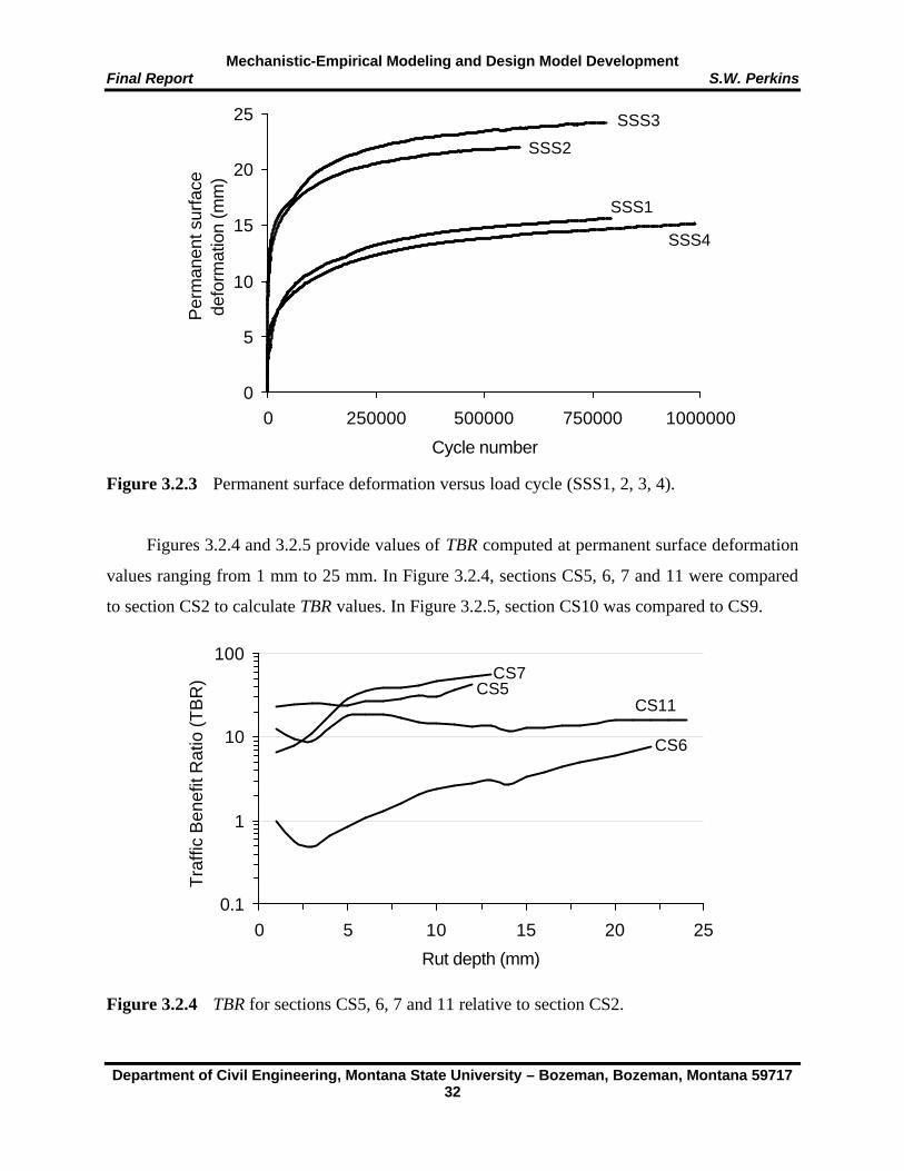
Mechanistic-Empirical Modeling and Design Model Development Final Report S.W. Perkins
Department of Civil Engineering, Montana State University – Bozeman, Bozeman, Montana 59717 32
Figure 3.2.3 Permanent surface deformation versus load cycle (SSS1, 2, 3, 4).
Figures 3.2.4 and 3.2.5 provide values of TBR computed at permanent surface deformation
values ranging from 1 mm to 25 mm. In Figure 3.2.4, sections CS5, 6, 7 and 11 were compared
to section CS2 to calculate TBR values. In Figure 3.2.5, section CS10 was compared to CS9.
Figure 3.2.4 TBR for sections CS5, 6, 7 and 11 relative to section CS2.
0
5
10
15
20
25
0 250000 500000 750000 1000000
Cycle number
Per
man
ent s
urfa
cede
form
atio
n (m
m)
SSS3
SSS1
SSS2
SSS4
0.1
1
10
100
0 5 10 15 20 25
Rut depth (mm)
Tra
ffic
Ben
efit
Rat
io (T
BR
) g
CS6
CS7
CS11CS5
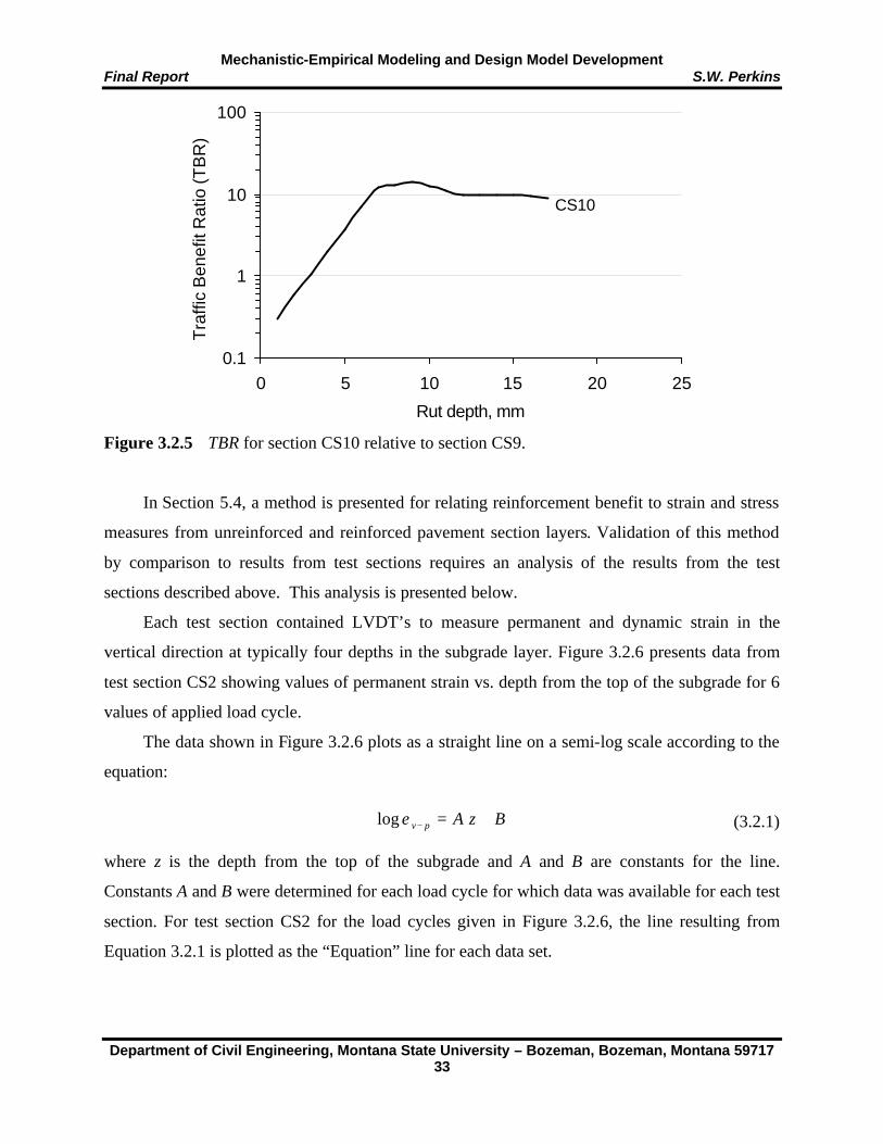
Mechanistic-Empirical Modeling and Design Model Development Final Report S.W. Perkins
Department of Civil Engineering, Montana State University – Bozeman, Bozeman, Montana 59717 33
BzApv +=−εlog
Figure 3.2.5 TBR for section CS10 relative to section CS9.
In Section 5.4, a method is presented for relating reinforcement benefit to strain and stress
measures from unreinforced and reinforced pavement section layers. Validation of this method
by comparison to results from test sections requires an analysis of the results from the test
sections described above. This analysis is presented below.
Each test section contained LVDT’s to measure permanent and dynamic strain in the
vertical direction at typically four depths in the subgrade layer. Figure 3.2.6 presents data from
test section CS2 showing values of permanent strain vs. depth from the top of the subgrade for 6
values of applied load cycle.
The data shown in Figure 3.2.6 plots as a straight line on a semi-log scale according to the
equation:
(3.2.1)
where z is the depth from the top of the subgrade and A and B are constants for the line.
Constants A and B were determined for each load cycle for which data was available for each test
section. For test section CS2 for the load cycles given in Figure 3.2.6, the line resulting from
Equation 3.2.1 is plotted as the “Equation” line for each data set.
0.1
1
10
100
0 5 10 15 20 25
Rut depth, mm
Tra
ffic
Ben
efit
Rat
io (T
BR
) q
CS10
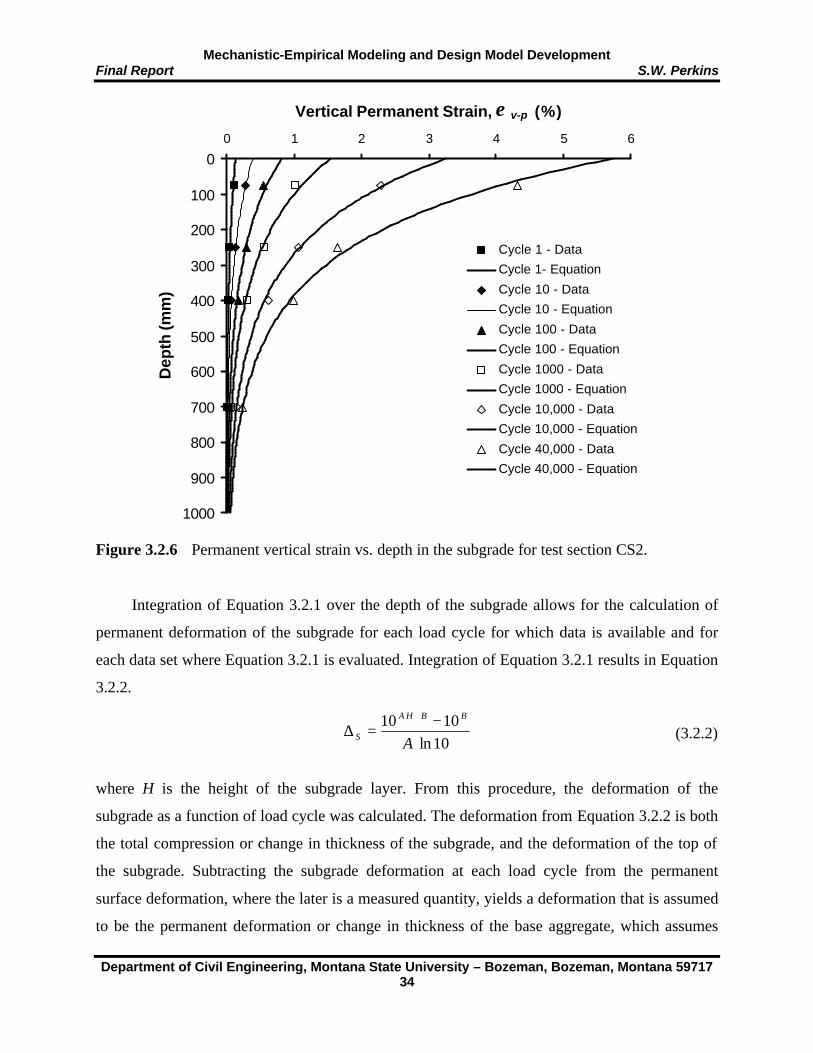
Mechanistic-Empirical Modeling and Design Model Development Final Report S.W. Perkins
Department of Civil Engineering, Montana State University – Bozeman, Bozeman, Montana 59717 34
10ln1010
A
BBHA
S−
=∆+
Figure 3.2.6 Permanent vertical strain vs. depth in the subgrade for test section CS2.
Integration of Equation 3.2.1 over the depth of the subgrade allows for the calculation of
permanent deformation of the subgrade for each load cycle for which data is available and for
each data set where Equation 3.2.1 is evaluated. Integration of Equation 3.2.1 results in Equation
3.2.2.
(3.2.2)
where H is the height of the subgrade layer. From this procedure, the deformation of the
subgrade as a function of load cycle was calculated. The deformation from Equation 3.2.2 is both
the total compression or change in thickness of the subgrade, and the deformation of the top of
the subgrade. Subtracting the subgrade deformation at each load cycle from the permanent
surface deformation, where the later is a measured quantity, yields a deformation that is assumed
to be the permanent deformation or change in thickness of the base aggregate, which assumes
0
100
200
300
400
500
600
700
800
900
1000
0 1 2 3 4 5 6
Vertical Permanent Strain, ε v-p (%)
Dep
th (m
m)
Cycle 1 - Data
Cycle 1- Equation
Cycle 10 - Data
Cycle 10 - Equation
Cycle 100 - Data
Cycle 100 - Equation
Cycle 1000 - Data
Cycle 1000 - Equation
Cycle 10,000 - Data
Cycle 10,000 - Equation
Cycle 40,000 - Data
Cycle 40,000 - Equation
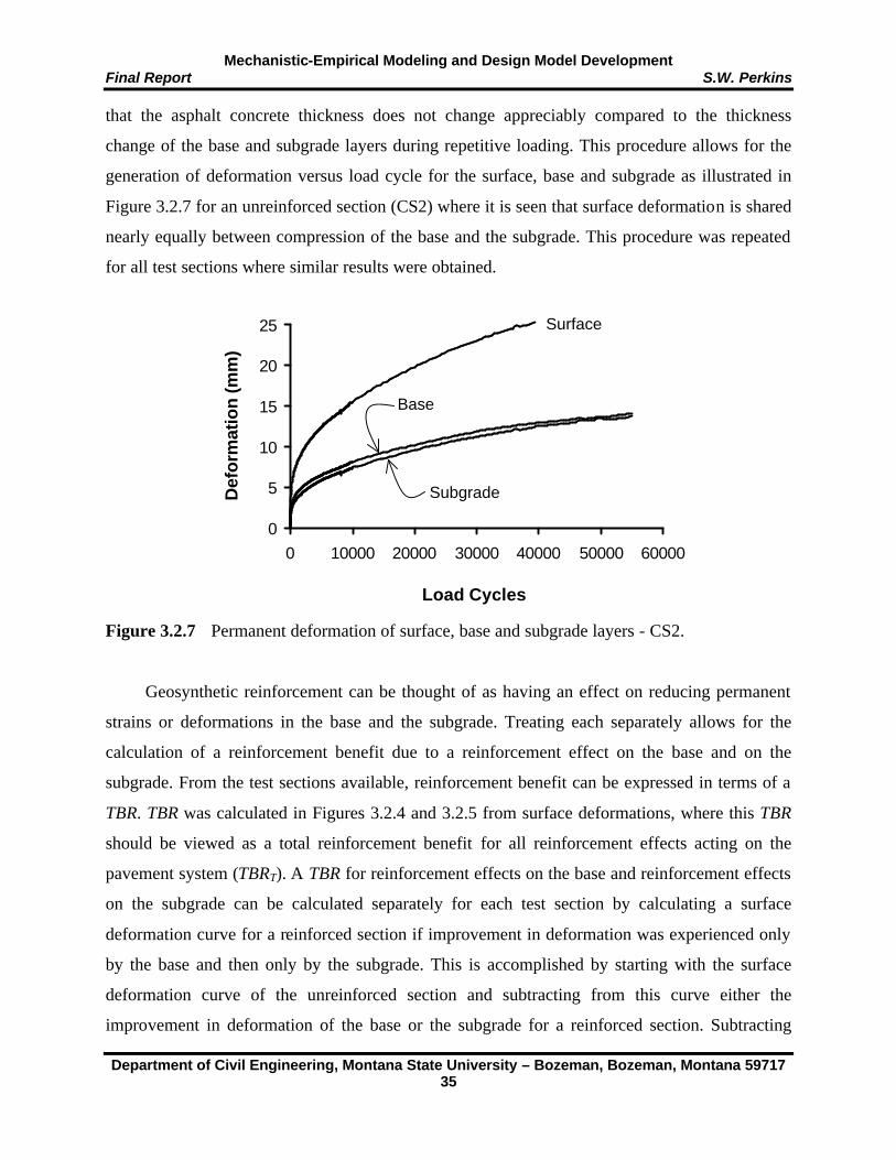
Mechanistic-Empirical Modeling and Design Model Development Final Report S.W. Perkins
Department of Civil Engineering, Montana State University – Bozeman, Bozeman, Montana 59717 35
that the asphalt concrete thickness does not change appreciably compared to the thickness
change of the base and subgrade layers during repetitive loading. This procedure allows for the
generation of deformation versus load cycle for the surface, base and subgrade as illustrated in
Figure 3.2.7 for an unreinforced section (CS2) where it is seen that surface deformation is shared
nearly equally between compression of the base and the subgrade. This procedure was repeated
for all test sections where similar results were obtained.
Figure 3.2.7 Permanent deformation of surface, base and subgrade layers - CS2.
Geosynthetic reinforcement can be thought of as having an effect on reducing permanent
strains or deformations in the base and the subgrade. Treating each separately allows for the
calculation of a reinforcement benefit due to a reinforcement effect on the base and on the
subgrade. From the test sections available, reinforcement benefit can be expressed in terms of a
TBR. TBR was calculated in Figures 3.2.4 and 3.2.5 from surface deformations, where this TBR
should be viewed as a total reinforcement benefit for all reinforcement effects acting on the
pavement system (TBRT). A TBR for reinforcement effects on the base and reinforcement effects
on the subgrade can be calculated separately for each test section by calculating a surface
deformation curve for a reinforced section if improvement in deformation was experienced only
by the base and then only by the subgrade. This is accomplished by starting with the surface
deformation curve of the unreinforced section and subtracting from this curve either the
improvement in deformation of the base or the subgrade for a reinforced section. Subtracting
0
5
10
15
20
25
0 10000 20000 30000 40000 50000 60000
Load Cycles
Def
orm
atio
n (m
m)
Base
Subgrade
Surface
Mechanistic-Empirical Modeling and Design Model Development Final Report S.W. Perkins
Department of Civil Engineering, Montana State University – Bozeman, Bozeman, Montana 59717 36
( )RBUBUBR −−− ∆−∆−∆=∆
both the improvement of the base and subgrade from the unreinforced surface deformation curve
results in the measured surface deformation curve of the reinforced section. This is accomplished
by applying Equations 3.2.3 and 3.2.4 for each load cycle where data is available and using
Equation 3.2.5 as a check.
(3.2.3)
(3.2.4)
(3.2.5)
where:
∆R-B = Calculated surface deformation for reinforced pavement assuming reinforcement
reduces only deformations in the base layer.
∆R-S = Calculated surface deformation for reinforced pavement assuming reinforcement
reduces only deformations in the subgrade layer.
∆U = Measured surface deformation of unreinforced section.
∆R = Measured surface deformation of reinforced section
∆B-U = Deformation of base layer for the unreinforced section.
∆B-R = Deformation of base layer for the reinforced section.
∆S-U = Deformation of subgrade layer for the unreinforced section.
∆S-R = Deformation of subgrade layer for the reinforced section.
Figure 3.2.8 shows an example from a reinforced section (CS11) showing the calculation of
these curves. At a given permanent surface deformation level (12.5 mm as in the case of Figure
3.2.8) a partial TBR can be computed for reinforcement effects on the base and on the subgrade
(TBRB, TBRS) by dividing the number of load cycles necessary to reach 12.5 mm of deformation
from the respective calculated curves for base and subgrade reinforcement by the corresponding
load cycles for the measured unreinforced curve. For this test section, the following numbers
were obtained: TBRT = 13.5, TBRB = 3.01, TBRS = 2.61, where all measurements were made at a
level of 12.5 mm. Carrying out these computations for all test sections results in values of TBR
measured at 12.5 mm of permanent surface deformation given in Table 3.2.1.
( )RSUSUSR −−− ∆−∆−∆=∆
( )RSUSRBUBUR −−−− ∆−∆+∆−∆−∆=∆
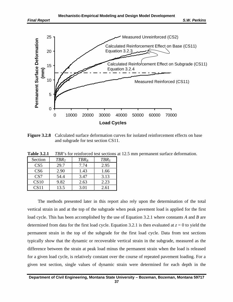
Mechanistic-Empirical Modeling and Design Model Development Final Report S.W. Perkins
Department of Civil Engineering, Montana State University – Bozeman, Bozeman, Montana 59717 37
Figure 3.2.8 Calculated surface deformation curves for isolated reinforcement effects on base
and subgrade for test section CS11.
Table 3.2.1 TBR’s for reinforced test sections at 12.5 mm permanent surface deformation. Section TBRT TBRB TBRS
CS5 29.7 7.74 2.95 CS6 2.90 1.43 1.66 CS7 54.4 3.47 3.13
CS10 9.82 2.63 2.23 CS11 13.5 3.01 2.61
The methods presented later in this report also rely upon the determination of the total
vertical strain in and at the top of the subgrade when peak pavement load is applied for the first
load cycle. This has been accomplished by the use of Equation 3.2.1 where constants A and B are
determined from data for the first load cycle. Equation 3.2.1 is then evaluated at z = 0 to yield the
permanent strain in the top of the subgrade for the first load cycle. Data from test sections
typically show that the dynamic or recoverable vertical strain in the subgrade, measured as the
difference between the strain at peak load minus the permanent strain when the load is released
for a given load cycle, is relatively constant over the course of repeated pavement loading. For a
given test section, single values of dynamic strain were determined for each depth in the
0
5
10
15
20
25
0 10000 20000 30000 40000 50000 60000 70000
Load Cycles
Per
man
ent S
urf
ace
Def
orm
atio
n
(mm
)Measured Unreinforced (CS2)
Calculated Reinforcement Effect on Base (CS11) Equation 3.2.3
Calculated Reinforcement Effect on Subgrade (CS11) Equation 3.2.4
Measured Reinforced (CS11)

Mechanistic-Empirical Modeling and Design Model Development Final Report S.W. Perkins
Department of Civil Engineering, Montana State University – Bozeman, Bozeman, Montana 59717 38
subgrade where LVDT’s were located by averaging the dynamic strain recorded for each load
cycle. Plotting these values versus depth showed that an equation of the same form as Equation
3.2.1 fit the data well. Figure 3.2.9 shows an example of this data for test section CS2. Dynamic
strain at the top of the subgrade was then added to the permanent strain at the top of the subgrade
for the first load cycle to give the total strain at the top of the subgrade for the first load cycle,
with results for each test section summarized in Table 3.2.2. Also shown in this table is the
number of load cycles necessary to reach 12.5 mm of permanent surface deformation. For the
unreinforced test sections (SSS1, SSS4, CS2, CS9) the values reported are directly from
measured surface deformation from the test sections. For the reinforced sections, the numbers
given are for permanent surface deformations computed for reinforcement effects occurring only
within the subgrade layer according to Equation 3.2.4 and as illustrated for reinforced test section
CS11 in Figure 3.2.8. This has been done to associate reinforcement benefit on the subgrade with
a response measure pertinent to the subgrade. The load cycle numbers shown in Table 3.2.2 were
the values used to produce the values for TBRS given in Table 3.2.1.
Figure 3.2.9 Measured dynamic strain versus depth and best fit line per Equation 3.2.1 for test
section CS2.
0
100
200
300
400
500
600
700
800
900
1000
0 0.2 0.4 0.6 0.8
Dynamic Strain (%)
Dep
th (m
m)

Mechanistic-Empirical Modeling and Design Model Development Final Report S.W. Perkins
Department of Civil Engineering, Montana State University – Bozeman, Bozeman, Montana 59717 39
Bvmm AN −= ε5.12
Values of total vertical strain in the top of the subgrade for the first load cycle were plotted
against the number of load cycles necessary for 12.5 mm of permanent surface deformation from
Table 3.2.2 (Figure 3.2.10). A best fit line of the form given in Equation 3.2.6, where A and B are
constants, and where εv is in decimal form, produced values of A = 1.8×10⁻⁵ and B = -4.07.
(3.2.6)
Equation 3.2.6 is commonly referred to as a subgrade rutting model for flexible pavements
with values for B as reported by four agencies ranging from 3.95 to 4.48 and values of A ranging
from 6.15×10⁻⁷ to 1.36×10⁻⁹ (Huang, 1993). Information from Table 3.2.1 and Equation 3.2.6 is
used later in Sections 5 and 7 for development of the design model.
Table 3.2.2 Total vertical strain at peak load for the first load cycle.
Section Total Vertical Strain (%) Load Cycles for 12.5 mm Permanent Surface Deformation SSS1 0.266 195,000 SSS4 0.272 263,000 CS2 0.843 5140 CS5 0.618 15,200 CS6 0.753 8550 CS7 0.584 16,100 CS9 0.712 12,500
CS10 0.559 27,900 CS11 0.680 13,400
4.0 PAVEMENT LAYER MATERIAL MODELS AND CALIBRATION TESTS
As discussed in Section 1.0, the numerical finite element model developed as part of this work
was designed to be used for the extraction of key stress and strain measures from the pavement
layers when one cycle of pavement load is applied. These mechanistic response measures are
then used in empirical distress models to quantify long-term pavement performance and
reinforcement benefit. The purpose of this section is to describe the material models developed
for the various pavement layers and the laboratory tests used to calibrate these models. The
relationship of material properties used in these models to commonly used pavement layer
material properties is also presented. It should be recognized that the majority of the material
parameters contained in the models for the various pavement materials described below are not

Mechanistic-Empirical Modeling and Design Model Development Final Report S.W. Perkins
Department of Civil Engineering, Montana State University – Bozeman, Bozeman, Montana 59717 40
contained in the design model described in Sections 7 and 8, and Appendix B. The properties
contained in the material models described in this section were developed for the purposes of
establishing the finite element model, which was used in the parametric study to quantify
reinforcement benefit as a function of a smaller and easily identifiable subset of pavement and
geosynthetic properties and characteristics.
Figure 3.2.10 Total vertical strain in top of the subgrade for the first load cycle versus number
of load cycles to reach 12.5 mm of permanent surface deformation.
4.1 Asphalt Concrete
Mechanistic-empirical flexible pavement models commonly use isotropic, linearly-elastic
material models for the asphalt concrete. Initially, such a model was adapted for use in this study
for sake of simplicity and for ease of comparison to other studies. Given the need to examine
permanent strains, however, in the subgrade after one load application, a material model for the
asphalt concrete that allowed for the development of permanent strain upon release of the load
was required. Otherwise, the elastic rebound of the asphalt concrete layer would create artificial
vertical tensile stresses and strains in the top of the aggregate layer. A plasticity component was
added to the model to allow for the development of permanent strain. The plasticity was
introduced by specification of an ultimate yield stress corresponding to a perfect plasticity
hardening law.
1000
10000
100000
1000000
0.001 0.003 0.005 0.007 0.009
Total Vertical Strain Top of Subgrade, εv (mm/mm)
Cyc
le N
um
ber
for
12.5
mm
S
urf
ace
Def
orm
atio
n, N
12.5
mm

Mechanistic-Empirical Modeling and Design Model Development Final Report S.W. Perkins
Department of Civil Engineering, Montana State University – Bozeman, Bozeman, Montana 59717 41
Incorporation of this material model into the finite element model described in Section 5
showed that vertical stresses in the subgrade close to the centerline of the load plate tended to be
under predicted, while vertical stresses at a radius greater than approximately 300 mm tended to
be over predicted. In addition, the predicted deflected shape of the asphalt surface tended to be
more flat than that seen from test section results. These findings suggested that the use of
isotropic elastic and plastic properties for the asphalt concrete tended to cause this layer to act
too much like an elastic slab distributing the stress too broadly. For these reasons, direction
dependency, or anisotropy, was added for the elastic and plastic properties. The addition of
anisotropy essentially allowed for the reduction of the flexural stiffness of the asphalt layer while
maintaining the vertical stiffness in compression.
Direction dependence of elastic properties was prescribed through the use of a linear,
orthotropic elastic constitutive matrix. Orthotropic linear elasticity is described by three moduli
(Eij), three independent Poisson’s ratios (νij) and three shear moduli (Gij), resulting in the elastic
constitutive matrix
(4.1.1)
where the subscripts x and y denote the in-plane horizontal directions, and z denotes the vertical
direction. Plasticity was described in terms of an ultimate yield stress, σ0AC, and six plastic
potential ratios, Rij, given in Equation 4.1.2, whose values are typically less than one and
describe the reduction in yield stress in each respective direction.
(4.1.2)
−−−−−−
=
yz
xz
xy
z
y
x
yz
xz
xy
yyyzxxz
zzyyxxy
zzxyyxx
yz
xz
xy
z
y
x
GG
GEEE
EEEEEE
τττσσσ
νννννν
γγγεεε
/1000000/1000000/1000000/1//000//1/000///1
=
yz
xz
xy
z
y
x
ACo
yz
xz
xy
z
y
x
RRRRRR
τττ
σσσ
σ
333
1

Mechanistic-Empirical Modeling and Design Model Development Final Report S.W. Perkins
Department of Civil Engineering, Montana State University – Bozeman, Bozeman, Montana 59717 42
Values of elastic modulus (Ez), Poisson’s ratio and yield stress (σ0AC) in the principal
direction of loading (i.e. the z-direction) were determined by conducting indirect tension (IDT)
resilient modulus tests per ASTM D4123 (ASTM, 2001b), where these tests were performed at
the Asphalt Institute, Lexington, Kentucky. Tests were performed on 150 mm diameter samples
cored from the test sections described in Section 3. Four 150 mm diameter cores were typically
taken from each test section upon the completion of the tests and were taken from areas outside
the footprint of the load plate. An additional six 100 mm cores were also obtained. Percent air
voids was determined for each core with the average air voids computed. Resilient modulus was
typically determined for two 150 mm cores from most sections. These cores were chosen to
bracket as closely as possible the average air voids for the test section. Resilient modulus tests
were performed at the average room temperature existing during the time the corresponding test
section was loaded and were performed at three frequencies of loading (0.33, 0.5 and 1 Hz) and
at two test positions corresponding to a 90 degree rotation. At the end of resilient modulus
testing, the samples were loaded to failure to determine the ultimate strength of each core.
Values of resilient modulus and Poisson’s ratio are reported in Table 4.1.1 and are average
values from each test rotation and testing frequency.
The IDT test results show a strong dependency on test specimen temperature and a lesser
dependence on specimen air voids. The dependence on air voids appears to become stronger as
the test temperature decreases. Given the consistency between certain sets of results from the test
sections, it would appear that the difference in actual temperature in the asphalt concrete during
the period over which pavement loading occurred between test sections is less than that implied
by the values of room temperature reported in Tables 3.1.3 and 4.1.1. For instance, test sections
CS2 and CS8 were identical unreinforced test sections that displayed nearly identical pavement
loading performance. The differences in room temperature for the two tests was reported as 7
degrees C. The IDT tests performed at this temperature difference resulted in a significant
difference in modulus of the AC, which did not appear to be evident from the test section results.
It is believed that the differences in actual AC temperature in the test sections was moderated by
the presence of the large body of soil upon which AC rested and is less than that implied by
room temperature measurements. Given the relatively small differences in average air voids
between the sections and the uncertainty regarding the true temperature of the asphalt concrete
during testing, typical values of modulus, Poisson’s ratio and ultimate tensile strength were used

Mechanistic-Empirical Modeling and Design Model Development Final Report S.W. Perkins
Department of Civil Engineering, Montana State University – Bozeman, Bozeman, Montana 59717 43
for all test section modeling. A value of modulus for Ez of 2500 MPa, a Poisson’s ratio of 0.35
and a yield strength of 675 kPa were chosen. A modulus of 2500 MPa corresponds
approximately to a structural layer coefficient of 0.4 corresponding to AASHTO (1993). Values
of the other parameters in Equations 4.1.1 and 4.1.2 as used in the finite element model for
modeling all cases examined are given in Table 4.1.2. The selection of the remaining values
shown in Table 4.1.2 was based on matching as closely as possible the vertical stresses observed
in the test sections.
Table 4.1.1 Indirect tension resilient modulus test results. Test
Section IDT Test
Temperature (degree C)
Specimen Air Voids
(%)
Average Resilient
Modulus (MPa)
Average Poisson’s
Ratio
Ultimate Tensile
Strength (kPa) SSS3-1 15 2.93 4583 0.34 1273 SSS3-3 16 4.17 3748 0.34 1009 SSS3-4 15 5.32 3032 0.30 938 SSS4-1 15 4.25 4519 0.26 1218 SSS4-2 15 3.38 4596 0.31 1288 SSS4-4 16 5.57 2826 0.15 888 CS2-3 17 1.97 3668 0.42 828 CS2-4 17 1.97 4094 0.36 901 CS5-3 24 5.12 1150 0.22 585 CS6-2 21 2.47 1934 0.35 604 CS7-1 24 4.46 1741 0.31 538 CS7-3 24 2.66 2049 0.41 581 CS8-2 24 2.87 1723 0.38 567 CS9-2 26 4.09 1356 0.41 447 CS9-4 26 6.10 1188 0.33 468 CS10-2 18 2.96 2944 0.42 977 CS11-1 25 1.23 1796 0.95 449 CS11-4 25 1.88 1538 0.32 441
4.2 Base Aggregate and Subgrade
The constitutive model used for both the base aggregate and the subgrade soil is based on the
bounding surface concept originally developed by Dafalias (1975) and extended for the
description of isotropic cohesive soils by Dafalias and Hermann (1982) and later updated by
Dafalias and Hermann (1986). The model was originally selected and incorporated into the finite
element model used in this study to provide a material model capable of showing the
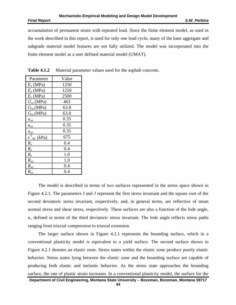
Mechanistic-Empirical Modeling and Design Model Development Final Report S.W. Perkins
Department of Civil Engineering, Montana State University – Bozeman, Bozeman, Montana 59717 44
accumulation of permanent strain with repeated load. Since the finite element model, as used in
the work described in this report, is used for only one load cycle, many of the base aggregate and
subgrade material model features are not fully utilized. The model was incorporated into the
finite element model as a user defined material model (UMAT).
Table 4.1.2 Material parameter values used for the asphalt concrete.
Parameter Value Ex (MPa) 1250 Ey (MPa) 1250 Ez (MPa) 2500 Gxy (MPa) 463 Gxz (MPa) 63.8 Gyz (MPa) 63.8 νxy 0.35 νxz 0.35 νyz 0.35 σ0
AC (kPa) 675 Rx 0.4 Ry 0.4 Rz 1.0 Rxy 1.0 Rxz 0.4 Ryz 0.4
The model is described in terms of two surfaces represented in the stress space shown in
Figure 4.2.1. The parameters I and J represent the first stress invariant and the square root of the
second deviatoric stress invariant, respectively, and, in general terms, are reflective of mean
normal stress and shear stress, respectively. These surfaces are also a function of the lode angle,
α, defined in terms of the third deviatoric stress invariant. The lode angle reflects stress paths
ranging from triaxial compression to triaxial extension.
The larger surface shown in Figure 4.2.1 represents the bounding surface, which in a
conventional plasticity model is equivalent to a yield surface. The second surface shown in
Figure 4.2.1 denotes an elastic zone. Stress states within the elastic zone produce purely elastic
behavior. Stress states lying between the elastic zone and the bounding surface are capable of
producing both elastic and inelastic behavior. As the stress state approaches the bounding
surface, the rate of plastic strain increases. In a conventional plasticity model, the surface for the

Mechanistic-Empirical Modeling and Design Model Development Final Report S.W. Perkins
Department of Civil Engineering, Montana State University – Bozeman, Bozeman, Montana 59717 45
elastic zone is coincidental with the bounding surface, meaning that stress states lying below the
current yield surface always produce purely elastic behavior.
Figure 4.2.1 Schematic illustration of the bounding surface plasticity model.
A radial mapping rule is used to locate a point on the bounding surface corresponding to
some state of stress inside or on the bounding surface. This mapping rule is illustrated by the
dashed line in Figure 4.2.1 having an origin on the I axis at the value CIo, where C is a material
parameter and Io is defined below. This mapping rule is necessary to prescribe yielding
characteristics determined from the image point on the bounding surface to the current state of
stress.
The bounding surface concept is general and permits the inclusion of any type of
formulation for a yield surface, which is taken to represent the formulation for the bounding
surface. The bounding surface used in the current model consists of three segments, as illustrated
in Figure 4.2.1. The adoption of a combined surface allows greater flexibility in assigning
behavior within the tension region of the stress space, the importance of which is discussed
below. The bounding surface model used for the base aggregate and the subgrade soil uses a
yield surface formulation extended from critical state soil mechanics models (Schofield and
Wroth, 1968). A critical state line, defining the failure state of the material, is given by a line
with a slope of N, where N is a function of the lode angle and is related to the slope of the critical
Ellipse1
Ellipse2
Hyperbola
r r/sp
CI0 I0/R
N(α) AI0
I0 TI0
Elastic Zone
CSL
0
J
I
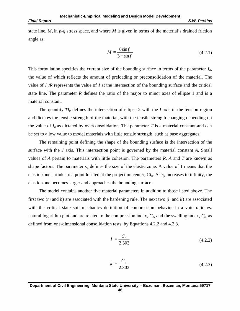
Mechanistic-Empirical Modeling and Design Model Development Final Report S.W. Perkins
Department of Civil Engineering, Montana State University – Bozeman, Bozeman, Montana 59717 46
φφ
sin3sin6
−=M
303.2cC
=λ
303.2sC
=κ
state line, M, in p-q stress space, and where M is given in terms of the material’s drained friction
angle as
(4.2.1)
This formulation specifies the current size of the bounding surface in terms of the parameter Io,
the value of which reflects the amount of preloading or preconsolidation of the material. The
value of Io/R represents the value of I at the intersection of the bounding surface and the critical
state line. The parameter R defines the ratio of the major to minor axes of ellipse 1 and is a
material constant.
The quantity TIo defines the intersection of ellipse 2 with the I axis in the tension region
and dictates the tensile strength of the material, with the tensile strength changing depending on
the value of Io as dictated by overconsolidation. The parameter T is a material constant and can
be set to a low value to model materials with little tensile strength, such as base aggregates.
The remaining point defining the shape of the bounding surface is the intersection of the
surface with the J axis. This intersection point is governed by the material constant A. Small
values of A pertain to materials with little cohesion. The parameters R, A and T are known as
shape factors. The parameter sp defines the size of the elastic zone. A value of 1 means that the
elastic zone shrinks to a point located at the projection center, CIo. As sp increases to infinity, the
elastic zone becomes larger and approaches the bounding surface.
The model contains another five material parameters in addition to those listed above. The
first two (m and h) are associated with the hardening rule. The next two (λ and κ) are associated
with the critical state soil mechanics definition of compression behavior in a void ratio vs.
natural logarithm plot and are related to the compression index, Cc, and the swelling index, Cs, as
defined from one-dimensional consolidation tests, by Equations 4.2.2 and 4.2.3.
(4.2.2)
(4.2.3)
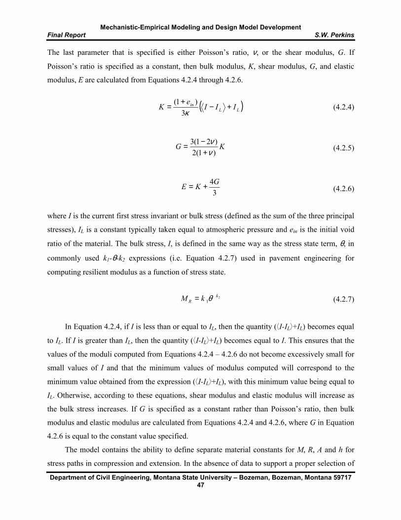
Mechanistic-Empirical Modeling and Design Model Development Final Report S.W. Perkins
Department of Civil Engineering, Montana State University – Bozeman, Bozeman, Montana 59717 47
KG)1(2)21(3
νν
+−=
34GKE +=
( )LLin III
eK +−
+=
κ3)1(
21
kR kM θ=
The last parameter that is specified is either Poisson’s ratio, ν, or the shear modulus, G. If
Poisson’s ratio is specified as a constant, then bulk modulus, K, shear modulus, G, and elastic
modulus, E are calculated from Equations 4.2.4 through 4.2.6.
(4.2.4)
(4.2.5)
(4.2.6)
where I is the current first stress invariant or bulk stress (defined as the sum of the three principal
stresses), IL is a constant typically taken equal to atmospheric pressure and ein is the initial void
ratio of the material. The bulk stress, I, is defined in the same way as the stress state term, θ, in
commonly used k1-θ-k2 expressions (i.e. Equation 4.2.7) used in pavement engineering for
computing resilient modulus as a function of stress state.
(4.2.7)
In Equation 4.2.4, if I is less than or equal to IL, then the quantity (+I-IL,+IL) becomes equal
to IL. If I is greater than IL, then the quantity (+I-IL,+IL) becomes equal to I. This ensures that the
values of the moduli computed from Equations 4.2.4 – 4.2.6 do not become excessively small for
small values of I and that the minimum values of modulus computed will correspond to the
minimum value obtained from the expression (+I-IL,+IL), with this minimum value being equal to
IL. Otherwise, according to these equations, shear modulus and elastic modulus will increase as
the bulk stress increases. If G is specified as a constant rather than Poisson’s ratio, then bulk
modulus and elastic modulus are calculated from Equations 4.2.4 and 4.2.6, where G in Equation
4.2.6 is equal to the constant value specified.
The model contains the ability to define separate material constants for M, R, A and h for
stress paths in compression and extension. In the absence of data to support a proper selection of
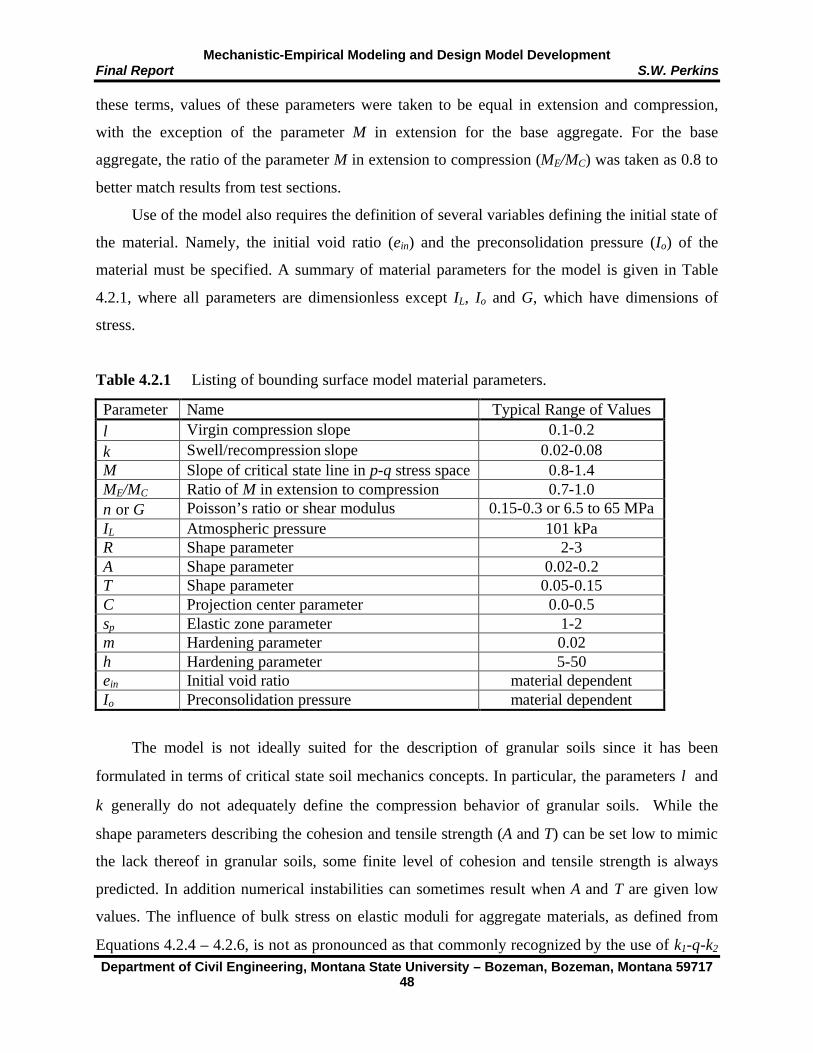
Mechanistic-Empirical Modeling and Design Model Development Final Report S.W. Perkins
Department of Civil Engineering, Montana State University – Bozeman, Bozeman, Montana 59717 48
these terms, values of these parameters were taken to be equal in extension and compression,
with the exception of the parameter M in extension for the base aggregate. For the base
aggregate, the ratio of the parameter M in extension to compression (ME/MC) was taken as 0.8 to
better match results from test sections.
Use of the model also requires the definition of several variables defining the initial state of
the material. Namely, the initial void ratio (ein) and the preconsolidation pressure (Io) of the
material must be specified. A summary of material parameters for the model is given in Table
4.2.1, where all parameters are dimensionless except IL, Io and G, which have dimensions of
stress.
Table 4.2.1 Listing of bounding surface model material parameters.
Parameter Name Typical Range of Values λ Virgin compression slope 0.1-0.2 κ Swell/recompression slope 0.02-0.08 M Slope of critical state line in p-q stress space 0.8-1.4 ME/MC Ratio of M in extension to compression 0.7-1.0 ν or G Poisson’s ratio or shear modulus 0.15-0.3 or 6.5 to 65 MPa IL Atmospheric pressure 101 kPa R Shape parameter 2-3 A Shape parameter 0.02-0.2 T Shape parameter 0.05-0.15 C Projection center parameter 0.0-0.5 sp Elastic zone parameter 1-2 m Hardening parameter 0.02 h Hardening parameter 5-50 ein Initial void ratio material dependent Io Preconsolidation pressure material dependent
The model is not ideally suited for the description of granular soils since it has been
formulated in terms of critical state soil mechanics concepts. In particular, the parameters λ and
κ generally do not adequately define the compression behavior of granular soils. While the
shape parameters describing the cohesion and tensile strength (A and T) can be set low to mimic
the lack thereof in granular soils, some finite level of cohesion and tensile strength is always
predicted. In addition numerical instabilities can sometimes result when A and T are given low
values. The influence of bulk stress on elastic moduli for aggregate materials, as defined from
Equations 4.2.4 – 4.2.6, is not as pronounced as that commonly recognized by the use of k1-θ-k2

Mechanistic-Empirical Modeling and Design Model Development Final Report S.W. Perkins
Department of Civil Engineering, Montana State University – Bozeman, Bozeman, Montana 59717 49
( ) 2
3)1(
1C
LLin III
eCK +−
+=
κ
expressions. To overcome this limitation, Equation 4.2.4 was modified for only the base
aggregate material by adding two additional constants, C1 and C2, as given in Equation 4.2.8.
(4.2.8)
The constant C2 has the same effect as k2 in Equation 4.2.7, while the constant C1 can be set to a
value such that its combination with ein and κ produces the same effect as k1 in Equation 4.2.7.
The influence on elastic modulus as computed from Equation 4.2.6 by the use of Equation 4.2.8
is discussed later in this section as results of model calibration are presented.
Detailed steps required for calibration of the constants given in Table 4.2.1 are described in
Kaliakin et al. (1987). In general, calibration of the model requires that three consolidated-
undrained conventional triaxial compression tests be performed at three different levels of
overconsolidation ratio. Data from the hydrostatic compression portion of the tests is used to
calibrate the compression parameters of the model. Calibration of the model from these tests
resulted in the parameters given in Table 4.2.2. For the base aggregate and silty sand subgrade,
Poisson’s ratio was specified, meaning that shear modulus and the other elastic moduli were a
function of bulk stress. For the base aggregate, the parameter IL was set purposely low in order to
provide for a variation of modulus over all bulk stress levels. For the clay subgrade, a constant
shear modulus was selected. The value of IL was set purposely high in this case to ensure that
little variation in modulus occurred over the range of bulk stress expected in this layer. This
ensured that the values of modulus used by specification of the properties given in Table 4.2.2
were approximately constant for all levels of loading and for all points within the subgrade layer.
This is consistent with the manner in which this material was prepared in the test sections
described in Section 3 of this report. The value of shear modulus given in Table 4.2.2 was
selected, in part, by relating CBR for this material to resilient modulus though Equation 4.2.9
(Heukelom and Klomp, 1962), assuming that resilient modulus was equivalent to elastic or
Young’s modulus (Equation 4.2.10), and then calculating shear modulus from elastic modulus
and an assumed Poisson’s ratio of 0.5 (Equation 4.2.11), where a Poisson’s ratio of 0.5
represents saturated subgrade loaded in an undrained manner. This produces a value of shear
modulus of 5170 kPa when CBR = 1.5. Further support for the use of these values and their
relationship to resilient modulus values is described below.

Mechanistic-Empirical Modeling and Design Model Development Final Report S.W. Perkins
Department of Civil Engineering, Montana State University – Bozeman, Bozeman, Montana 59717 50
CBRpsiM R 1500)( =
CBRpsiMkPaE R 335,10)(89.6)( ==
CBRE
kPaG 3445)1(2
)( =+
=ν
(4.2.9)
(4.2.10)
(4.2.11)
Table 4.2.2 Calibrated bounding surface model parameters for test section materials.
Values Parameter Clay Subgrade Silty Sand Subgrade Base Aggregate
λ 0.225 0.022 0.007 κ 0.11 0.005 0.0018 M 0.65 1.6 1.8 ME/MC 1.0 1.0 0.8 ν - 0.2 0.3 G (kPa) 5170 - - IL (kPa) 600.0 101.4 0.3 R 2.0 1.4 2.3 A 0.02 0.02 0.02 T 0.05 0.01 0.01 C 0.3 0.0 0.3 sp 1.75 1.1 1.0 m 0.02 0.02 0.02 h 50.0 15 50.0 C1 1 1 40 C2 1 1 0.6 ein 1.30 – 1.39 0.537 – 0.547 0.223 – 0.259 Io (kPa) 225 750 450
Since the use of resilient modulus for the characterization of base aggregate and subgrade
materials is commonly used in pavement engineering, additional work was performed to evaluate
the range of resilient modulus values predicted by the model described above using the
parameters for the different materials given in Table 4.2.2. This was accomplished by using the
model to simulate the loading sequence, measurement of strains and calculation of resilient
modulus as used in the test specification for resilient modulus tests for aggregate and subgrade
soils per AASHTO T 292-91 (AASHTO, 1991). For the base aggregate material, the calculation
of resilient modulus from the model simulation results is plotted against bulk stress, θ, in Figure
4.2.2. The best-fit line in this Figure is from the use of Equation 4.2.7 with values of k1 = 4460

Mechanistic-Empirical Modeling and Design Model Development Final Report S.W. Perkins
Department of Civil Engineering, Montana State University – Bozeman, Bozeman, Montana 59717 51
and k2 = 0.63, when θ and MR are in units of psi. According to AASHTO (1993), these values
represent a typical base aggregate that would be in a damp condition. Assuming a typical value
of θ of 20 psi in the base aggregate layer, a layer coefficient for the aggregate of 0.14 is obtained
from the AASHTO (1993) equations.
A similar simulation of the resilient modulus test was performed using model parameters
for the clay subgrade and silty-sand subgrade where an undrained simulation was performed for
the clay subgrade. For the clay subgrade, resilient modulus did not change appreciably with bulk
stress, as a result of the high value of IL used, and changed only moderately for the range of
deviatoric stress values used, giving an average value of resilient modulus of approximately 15.5
MPa (2260 psi). According to the Equation 4.2.9, commonly used for cohesive subgrades, this
corresponds to a CBR of 1.5, whereas the measured CBR for the clay subgrade from the test
sections was also 1.5. A similar simulation using the silty-sand subgrade parameters resulted in a
range of resilient modulus values from 18 to 29 MPa (2600 to 4200 psi) when following the
subgrade testing protocol and 14 to 140 MPa (2000 to 20,000 psi) when following the unbound
aggregate testing protocol. These results indicate that the bounding surface plasticity model used
for the base aggregate and subgrade soils provides a comparable description of elastic properties
commonly used in conventional pavement engineering practice.
Figure 4.2.2 Predicted resilient modulus values from base aggregate bounding surface model.
0
100
200
300
400
500
600
0 200 400 600 800
Bulk Stress, θ (kPa)
Res
ilien
t Mo
du
lus,
MR
(MP
a)

Mechanistic-Empirical Modeling and Design Model Development Final Report S.W. Perkins
Department of Civil Engineering, Montana State University – Bozeman, Bozeman, Montana 59717 52
4.3 Geosynthetics
A linear elastic, anisotropic model was used for the geosynthetic material. This type of model
was chosen for several reasons. The finite element model described in Section 5 was developed
to provide stress and strain response measures for one cycle of pavement load. Results from test
sections have indicated that the dynamic strain, or the strain for one load cycle, induced in the
geosynthetic is relatively small and is most likely within the elastic range for most geosynthetic
products. In addition, tension testing and data analysis protocols are not readily available for the
identification of material properties for more complex material models involving plasticity or
creep.
The finite element model described in Section 5 incorporates membrane elements for the
geosynthetic. These elements possess the property of having load carrying capacity in tension but
no capacity in compression and no resistance to bending. These elements are ideally suited for
describing the behavior of flexible sheets with little to no out-of-plane flexural stiffness.
Membrane elements with a thickness of 1 mm were used.
The anisotropic linear elastic model developed is given by Equation 4.3.1, where xm, m and
n correspond to the cross-machine, machine and normal directions, respectively, of the
geosynthetic. The model contains an elastic modulus for each principal material direction.
Response normal to the geosynthetic does not impact the material’s behavior, meaning that En is
chosen only to ensure stability of the elastic matrix. Values of elastic modulus are based on the
assumed 1 mm thickness of the material.
−−−−−−
=
−
−
−
−
−
−
−−
−−
−−
−
−
−
nm
nxm
mxm
n
m
xm
nm
nxm
mxm
nmnmxmnxm
nmnmxmmxm
nxmnmxmmxm
nm
nxm
mxm
n
m
xm
GG
GEEE
EEEEEE
τττ
σσσ
νννννν
γγγ
εεε
/1000000/1000000/1000000/1//000//1/000///1
(4.3.1)
Three independent Poisson’s ratios (νij) and three shear moduli (Gij) are contained in the
model. The three values of G are set equal to one another. The three Poisson’s ratios specified
are νxm-m, νxm-n and νm-n, where these are set equal to one another. The remaining three are
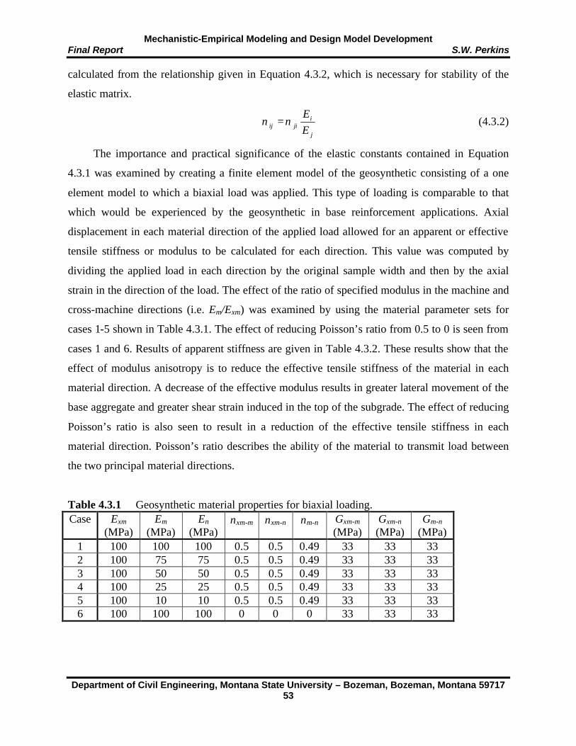
Mechanistic-Empirical Modeling and Design Model Development Final Report S.W. Perkins
Department of Civil Engineering, Montana State University – Bozeman, Bozeman, Montana 59717 53
calculated from the relationship given in Equation 4.3.2, which is necessary for stability of the
elastic matrix.
j
ijiij E
Eνν = (4.3.2)
The importance and practical significance of the elastic constants contained in Equation
4.3.1 was examined by creating a finite element model of the geosynthetic consisting of a one
element model to which a biaxial load was applied. This type of loading is comparable to that
which would be experienced by the geosynthetic in base reinforcement applications. Axial
displacement in each material direction of the applied load allowed for an apparent or effective
tensile stiffness or modulus to be calculated for each direction. This value was computed by
dividing the applied load in each direction by the original sample width and then by the axial
strain in the direction of the load. The effect of the ratio of specified modulus in the machine and
cross-machine directions (i.e. Em/Exm) was examined by using the material parameter sets for
cases 1-5 shown in Table 4.3.1. The effect of reducing Poisson’s ratio from 0.5 to 0 is seen from
cases 1 and 6. Results of apparent stiffness are given in Table 4.3.2. These results show that the
effect of modulus anisotropy is to reduce the effective tensile stiffness of the material in each
material direction. A decrease of the effective modulus results in greater lateral movement of the
base aggregate and greater shear strain induced in the top of the subgrade. The effect of reducing
Poisson’s ratio is also seen to result in a reduction of the effective tensile stiffness in each
material direction. Poisson’s ratio describes the ability of the material to transmit load between
the two principal material directions.
Table 4.3.1 Geosynthetic material properties for biaxial loading. Case Exm
(MPa) Em
(MPa) En
(MPa) νxm-m νxm-n νm-n Gxm-m
(MPa) Gxm-n
(MPa) Gm-n
(MPa) 1 100 100 100 0.5 0.5 0.49 33 33 33 2 100 75 75 0.5 0.5 0.49 33 33 33 3 100 50 50 0.5 0.5 0.49 33 33 33 4 100 25 25 0.5 0.5 0.49 33 33 33 5 100 10 10 0.5 0.5 0.49 33 33 33 6 100 100 100 0 0 0 33 33 33
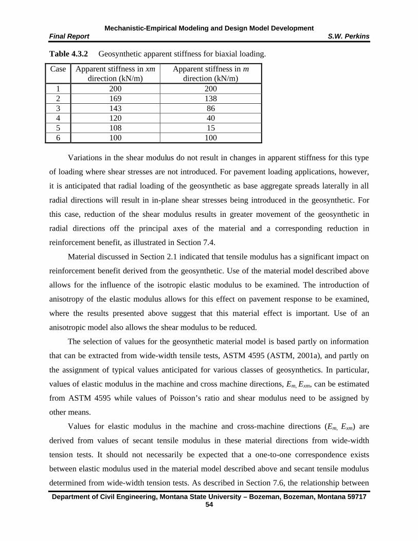
Mechanistic-Empirical Modeling and Design Model Development Final Report S.W. Perkins
Department of Civil Engineering, Montana State University – Bozeman, Bozeman, Montana 59717 54
Table 4.3.2 Geosynthetic apparent stiffness for biaxial loading.
Case Apparent stiffness in xm direction (kN/m)
Apparent stiffness in m direction (kN/m)
1 200 200 2 169 138 3 143 86 4 120 40 5 108 15 6 100 100
Variations in the shear modulus do not result in changes in apparent stiffness for this type
of loading where shear stresses are not introduced. For pavement loading applications, however,
it is anticipated that radial loading of the geosynthetic as base aggregate spreads laterally in all
radial directions will result in in-plane shear stresses being introduced in the geosynthetic. For
this case, reduction of the shear modulus results in greater movement of the geosynthetic in
radial directions off the principal axes of the material and a corresponding reduction in
reinforcement benefit, as illustrated in Section 7.4.
Material discussed in Section 2.1 indicated that tensile modulus has a significant impact on
reinforcement benefit derived from the geosynthetic. Use of the material model described above
allows for the influence of the isotropic elastic modulus to be examined. The introduction of
anisotropy of the elastic modulus allows for this effect on pavement response to be examined,
where the results presented above suggest that this material effect is important. Use of an
anisotropic model also allows the shear modulus to be reduced.
The selection of values for the geosynthetic material model is based partly on information
that can be extracted from wide-width tensile tests, ASTM 4595 (ASTM, 2001a), and partly on
the assignment of typical values anticipated for various classes of geosynthetics. In particular,
values of elastic modulus in the machine and cross machine directions, Em, Exm, can be estimated
from ASTM 4595 while values of Poisson’s ratio and shear modulus need to be assigned by
other means.
Values for elastic modulus in the machine and cross-machine directions (Em, Exm) are
derived from values of secant tensile modulus in these material directions from wide-width
tension tests. It should not necessarily be expected that a one-to-one correspondence exists
between elastic modulus used in the material model described above and secant tensile modulus
determined from wide-width tension tests. As described in Section 7.6, the relationship between

Mechanistic-Empirical Modeling and Design Model Development Final Report S.W. Perkins
Department of Civil Engineering, Montana State University – Bozeman, Bozeman, Montana 59717 55
these two parameters is established by comparison of predictions from the mechanistic-empirical
model to results from test sections.
The ratio between secant modulus from the two principal directions of the geosynthetic as
seen from wide-width tensile tests is maintained in the material model described above, but the
magnitude of the modulus values is not necessarily the same. Differences in magnitude are
expected for several reasons. The material model described above assumes a certain thickness for
the geosynthetic, which then governs the selection of elastic modulus. The finite element
response model using the geosynthetic material model described above is based on one load
application and is pertinent to a small strain response of the geosynthetic. Secant tensile modulus
from ASTM 4595 at values of axial strain less than 2 % are not commonly reported. Strains of 2
% in the geosynthetic for the first load application of a pavement are significantly higher than
what would normally be expected. Finally, the rate of load application is as much as 100 times
faster in the pavement application than in a wide-width tension test. The combination of these
effects suggests that the values of elastic modulus as used in Equation 4.3.1 should be expected
to be greater than values of secant tensile modulus determined from ASTM 4595.
Test methods for the definition of Poisson’s ratio and shear modulus, as defined in
Equation 4.3.1, do not currently exist. In addition, values for these two material properties for
various geosynthetics have not been reported. The design model, however, indicates that
reinforcement benefit is moderately sensitive to variations of these two parameters, as is
demonstrated in Section 7.4. Given the absence of test methods and typical values for these
properties, the design model described in Section 7 defines reinforcement benefit (or more
specifically a reduction factor applied to reinforcement benefit) in terms of two values for
Poisson’s ratio and two values for shear modulus, where these two values describe either good or
poor conditions for benefit.
The design model has been calibrated from test section results using two extruded geogrids
of the same manufacturing process and one woven geotextile. The calibration process involved
the assignment of either good or poor values for these properties such that benefit from the test
section results could be matched. As such, it is suggested that these two properties be related to
the geosynthetic type and structure. Additional results from test sections using a wider range of
geosynthetic products is necessary prior to being able to develop specific guidelines for selection
of these two properties. In the absence of these results, the values used for the two types of

Mechanistic-Empirical Modeling and Design Model Development Final Report S.W. Perkins
Department of Civil Engineering, Montana State University – Bozeman, Bozeman, Montana 59717 56
products used in test sections for which the design model was calibrated should be used as a
starting point. The qualitative application guidelines for geosynthetic type given in Table 2.1.2
derived from the GMA WPII (Berg et al., 2000) may also be used in the assignment of these
values.
Differences in interface shear properties may also be responsible for the differences in
pavement performance seen between various geosynthetics. As discussed in Section 2.1 and 2.6,
small displacement shear stiffness of the interface is most likely the key material parameter for
this component of the reinforced pavement system. Existing test protocols and test data are,
however, not currently available to explicitly define this property. The design model presented in
Section 7 uses a reduction factor for interface shearing resistance that has been calibrated for the
two types of geosynthetics used in previously constructed test sections. These values serve as a
starting point for geogrid and geotextile type materials. Further definition of this reduction factor
for other geosynthetic materials should come from additional test section results or from further
laboratory interface testing.
5.0 PAVEMENT TEST FACILITY FINITE ELEMENT MODEL
A finite element model was created to simulate the pavement layer thicknesses, boundary
conditions and loading present in the pavement test sections described in Section 3. All modeling
was done using the commercial program ABAQUS (Hibbitt, Karlson and Sorensen, 1998). Three
types of models were created. The first is a model of pavement test sections without
reinforcement and is described in Section 5.1. The second is a model where reinforcement is
described in such a way that it represents the maximum amount of reinforcement benefit that
could be expected with a “perfect” reinforcement product. Since effects of the reinforcement are
ultimately expressed in terms of prevention of lateral movement of the base aggregate at the
level of the geosynthetic, perfect reinforcement is simulated by modifying the unreinforced
model by preventing all in-plane or lateral motions of the base aggregate element nodes at the
level of the geosynthetic. This in effect simulates reinforcement with an infinitely stiff
geosynthetic and an infinitely stiff contact shear interface between the geosynthetic and the
aggregate. This model is described in Section 5.2. The third type of model created is one where a
separate material layer corresponding to the geosynthetic is added to the unreinforced model and
is described in Section 5.3.

Mechanistic-Empirical Modeling and Design Model Development Final Report S.W. Perkins
Department of Civil Engineering, Montana State University – Bozeman, Bozeman, Montana 59717 57
This approach of creating three types of finite element models was taken to describe the
effects of reinforcement in a systematic way that isolates the effects of each variable or group of
variables on the system. The unreinforced models provide response parameters for pavements
without any type of reinforcement, where these response parameters are described in Section 5.4.
The perfect reinforced models do not contain parameters associated with the geosynthetic. Any
benefit from the effect of the perfect reinforcement model is then a function of the remaining
pavement system variables, which include AC and base aggregate thickness, and subgrade
stiffness. From these results, conclusions can be made regarding the combinations of structural
section thickness and subgrade stiffness for which perfect reinforcement provides benefit. The
third type of model contains a reinforcement layer with corresponding material properties.
Variation of these properties allows for conclusions to be made regarding how those properties
modify or reduce the maximum benefit seen from the corresponding perfect reinforcement case.
Execution of models according to this approach minimizes the number of cases that need to be
analyzed and provides for a systematic method for interpreting the results.
5.1 Unreinforced FE Model
The finite element model of unreinforced pavements is a 3-dimensional model created to match
the nominal conditions for the pavement test facility described in Section 3. A two-dimensional
axi-symmetric model was not used because of the potential influence of the box’s square corners
and for the later inclusion of a layer of geosynthetic reinforcement that has direction dependent
material properties. Symmetry of the box was recognized such that a model of one-quarter of the
box was created. Figure 5.1.1 illustrates the geometry and boundary conditions used for the
development of the model. Actual layer thicknesses for the AC and base aggregate are described
in Section 6.
The width in the x and y directions of the ¼ box modeled was 1 m. The pavement load was
applied as a pressure equal to 550 kPa over one-quarter of a circular plate having a radius of 152
mm. The load plate and rubber pad used in the pavement test sections described in Section 3
were modeled by plates having a radius of 152 mm. The load plate had a thickness of 25 mm and
was given isotropic elastic properties with a Young’s modulus of 2×10⁸ kPa and a Poisson’s ratio
of 0.33. The rubber pad had a thickness of 4 mm and was also given elastic properties with a
Young’s modulus of 400 kPa and a Poisson’s ratio of 0. The pavement load was applied in a
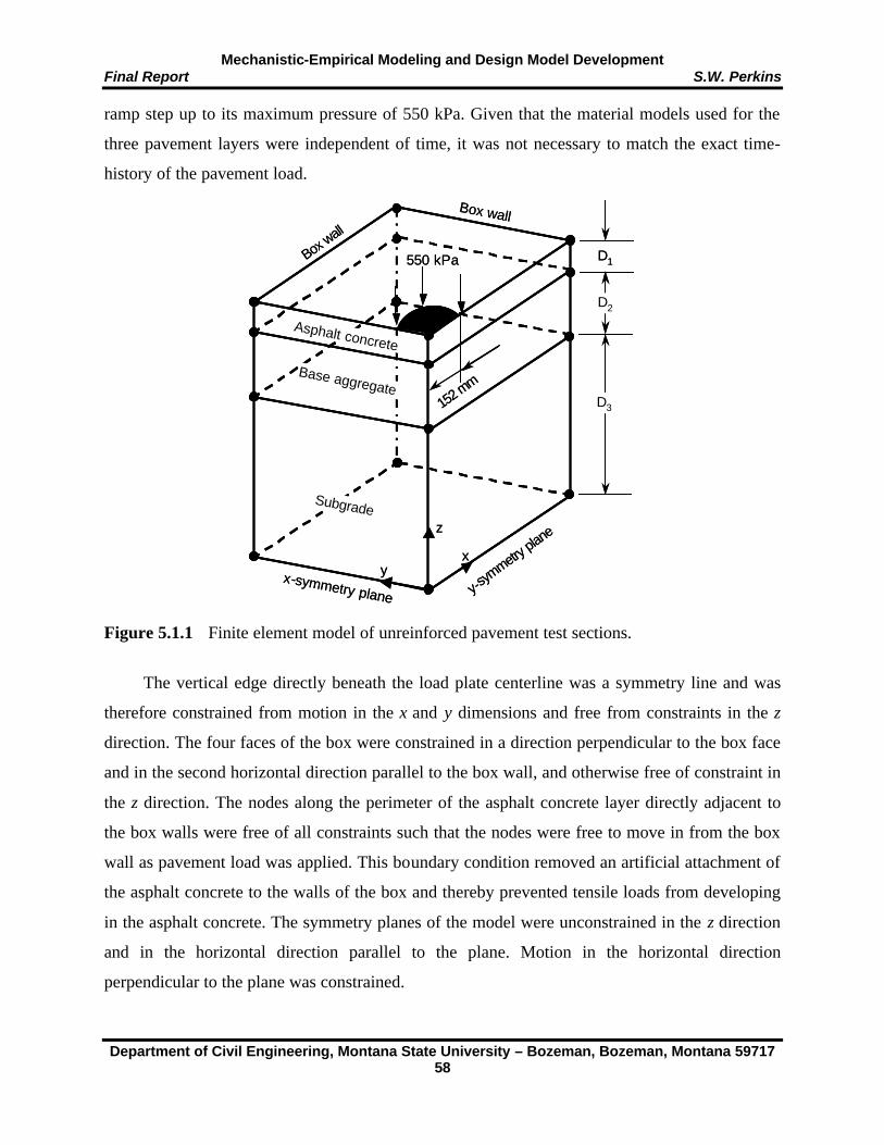
Mechanistic-Empirical Modeling and Design Model Development Final Report S.W. Perkins
Department of Civil Engineering, Montana State University – Bozeman, Bozeman, Montana 59717 58
ramp step up to its maximum pressure of 550 kPa. Given that the material models used for the
three pavement layers were independent of time, it was not necessary to match the exact time-
history of the pavement load.
Figure 5.1.1 Finite element model of unreinforced pavement test sections.
The vertical edge directly beneath the load plate centerline was a symmetry line and was
therefore constrained from motion in the x and y dimensions and free from constraints in the z
direction. The four faces of the box were constrained in a direction perpendicular to the box face
and in the second horizontal direction parallel to the box wall, and otherwise free of constraint in
the z direction. The nodes along the perimeter of the asphalt concrete layer directly adjacent to
the box walls were free of all constraints such that the nodes were free to move in from the box
wall as pavement load was applied. This boundary condition removed an artificial attachment of
the asphalt concrete to the walls of the box and thereby prevented tensile loads from developing
in the asphalt concrete. The symmetry planes of the model were unconstrained in the z direction
and in the horizontal direction parallel to the plane. Motion in the horizontal direction
perpendicular to the plane was constrained.
xy
z
Box wall
Box wall
Asphalt concrete
x-symmetry plane y-sym
metry pla
ne
Base aggregate
Subgrade
D1
D3
D2
550 kPa
152 mm
xy
z
Box wall
Box wall
Asphalt concrete
x-symmetry plane y-sym
metry pla
ne
Base aggregate
Subgrade
D1
D3
D2
550 kPa
152 mm

Mechanistic-Empirical Modeling and Design Model Development Final Report S.W. Perkins
Department of Civil Engineering, Montana State University – Bozeman, Bozeman, Montana 59717 59
Eight-noded hexagonal solid elements were used for all material layers. Approximately
42 elements were used for each of the load plate and rubber pad while 230, 570 and 1710
elements were used for the asphalt concrete, base aggregate and subgrade layers, respectively.
The nodes between the material layers were equivalenced and therefore connected.
5.2 Perfect Reinforced FE Model
In order to reduce the number of model cases analyzed under the parametric study described in
Section 6 and to provide for a systematic approach to interpreting results, a series of model cases
were analyzed where the reinforcement was modeled in such a way as to provide for the
maximum effect on pavement performance. Within the context of the material and finite element
models developed for this project, the principal effect of reinforcement on the performance of the
pavement is the prevention of lateral strain or displacement of the base aggregate at the interface
with the geosynthetic. Maximum effect of a reinforcement layer could thereby be simulated by
preventing all lateral motion of the base course aggregate at the level where it would be in
contact with the geosynthetic. This was accomplished by modifying the unreinforced model
described in Section 5.1 by prescribing boundary conditions to the nodes at the bottom of the
base aggregate, where these boundary conditions prevented all x and y motion of the nodes.
According to this approach, a geosynthetic layer was not explicitly included in this type of finite
element model.
For these models, the simulated reinforcement effectively has an infinite tensile stiffness
and an infinitely stiff contact interface with the base aggregate. The observation of reinforcement
benefit, or the lack thereof, was then due to the influence of pavement variables other than
geosynthetic properties. The variables associated with the pavement that are believed to have the
most significant influence on reinforcement benefit are thickness of the AC and base aggregate
layer and the properties of the subgrade dictating its stiffness and strength. This is a relatively
small number of variables in comparison to that which would be introduced if an actual layer of
reinforcement with its own set of material properties was introduced. Results from model cases
using the perfect reinforced model are used to make conclusions regarding the influence of the
structural section thickness and subgrade properties on reinforcement benefit. Additional work
with the model described in Section 5.3 is then used to modify and reduce reinforcement benefit
Mechanistic-Empirical Modeling and Design Model Development Final Report S.W. Perkins
Department of Civil Engineering, Montana State University – Bozeman, Bozeman, Montana 59717 60
observed for cases of perfect reinforcement by the influence of specific properties pertinent to
geosynthetics.
5.3 Geosynthetic Reinforced FE Model
A third type of finite element model was created where a sheet of geosynthetic reinforcement
was included as part of the pavement cross-section. The geosynthetic was modeled by 4 noded
membrane elements that have the property of containing tensile load carrying capacity, but have
no resistance in bending or compression. Membrane elements are two-dimensional elements that
are commonly used for describing flexible sheets having tensile load carrying capacity. The
material model described in Section 4.3 was used for the geosynthetic. In all cases, the
geosynthetic was placed between the base aggregate and the subgrade. The nodes of the
geosynthetic were equivalenced with the nodes in the base aggregate above and the subgrade
material below such that the three materials moved together as a unit. This approach isolates the
effect of geosynthetic material properties from those of interface properties. The effect of contact
interface properties is accounted for by comparison of model predictions where all other
properties have been accounted for to test section results. Remaining reductions in benefit are
then due to the influence of contract properties.
5.4 Response Parameters and Extension to Reinforcement Benefit
The types of models described in Sections 5.1 – 5.3 were executed with two response measures
extracted from the models to characterize pavement performance and eventually used to describe
reinforcement benefit. From material presented in Section 3.2, it was seen that reinforcement
benefit, defined in terms of an extension of life of the pavement, could be broken into
reinforcement effects on the base aggregate layer and on the subgrade layer. Partial traffic
benefit ratios for the base and subgrade (TBRB and TBRS) were defined and determined directly
from test section data for the various test sections available.
Test section data indicated that vertical strain in the top of the subgrade at peak load for the
first load cycle could be related to the number of load cycles necessary to reach 12.5 mm of
permanent surface deformation through a well-recognized subgrade rutting model (Huang,
1993). This model is given again in Equation 5.4.1, where the constants A and B were found to
be equal to 1.8×10⁻⁵ and 4.07, respectively, from the test sections reported in Section 3.

Mechanistic-Empirical Modeling and Design Model Development Final Report S.W. Perkins
Department of Civil Engineering, Montana State University – Bozeman, Bozeman, Montana 59717 61
Bvmm AN −= ε5.12
B
Uv
Rv
Umm
Rmm
NN
−
−
−
−
−
=
εε
5.12
5.12
B
Uv
RvSTBR
−
−
−
=
εε
(5.4.1)
If the vertical strain in Equation 5.4.1 is evaluated for comparison reinforced and unreinforced
pavement sections, then the ratio of the number of load cycles necessary to reach 12.5 mm of
permanent surface deformation will be given by Equation 5.4.2.
(5.4.2)
where the symbols R and U denote reinforced and unreinforced pavement sections. The ratio of
load cycles or vehicle passes necessary to reach 12.5 mm of surface deformation provides a
direct definition of TBR at this rut depth. Since this definition of TBR involves an effect of the
reinforcement only on the subgrade, the value is viewed as a partial TBR describing only
subgrade effects and is taken as the same TBRS defined in Section 3.2. According to this
formulation, the first response measure extracted from the models is the vertical compressive
strain in the top of the subgrade directly beneath the load plate centerline when the pavement
load has been fully applied for comparison reinforced and unreinforced test sections. Values of
vertical compressive strain are extrapolated from integration points within the first element in the
subgrade in order to extrapolate back to a value at the top of the subgrade. TBRS is then defined
from model response parameters by Equation 5.4.2
(5.4.2)
where B was calibrated from test section data and found to equal 4.07. The use of Equation 5.4.2
with the vertical strain results for the test sections given in Table 3.2.2 results in the values given
in Table 5.4.1, which are compared to the values of TBRS defined directly from load cycle
numbers reported in Table 3.2.2. Any discrepancies between the two values for a given test
section are due to the inability of Equation 5.4.2 to fully describe results seen from test sections,
where these discrepancies were shown previously in Figure 3.2.10.

Mechanistic-Empirical Modeling and Design Model Development Final Report S.W. Perkins
Department of Civil Engineering, Montana State University – Bozeman, Bozeman, Montana 59717 62
Table 5.4.1 TBRS for reinforced test sections.
Section TBRS (Table 3.2.1) TBRS (Equation 5.4.2) CS5 2.95 3.54 CS6 1.66 1.59 CS7 3.13 4.45
CS10 2.23 2.67 CS11 2.61 2.40
The second response measure extracted from the finite element models is a measure that
describes reinforcement effects on the base aggregate. It has been speculated that reinforcement
has the effect of providing confinement to the aggregate and thereby increasing bulk stress. An
increase in bulk stress has the effect of increasing stiffness of the base aggregate layer. Due to
the difficulties in measuring lateral stress and the difficulty of measuring stress components at
more than just several points within the base layer of test sections, this reinforcement mechanism
has not been verified experimentally but the direct effects of the mechanism have.
In the finite element models, bulk stress is extracted from a number of integration points
within the base aggregate layer when the full pavement load has been applied. Since bulk stress
changes from point to point within the aggregate layer, it is necessary to define a representative
or average value of bulk stress for the layer. The volume of aggregate used to define the average
is concentrated around and under the applied load since this is the material that is responsible for
spreading the load to the underlying subgrade. The geometry used to define the volume of
aggregate over which the bulk stress is averaged corresponds to a right frustum shown in Figure
5.4.1. Also shown on this figure are curves of normalized vertical stress at three depths in the
aggregate caused by a uniform pressure on the circular plate shown. The volume used is seen to
be an approximation of the zone of most significant stress intensity. It should be noted that
typical recommendations for the selection of bulk stress for use in the determination of resilient
modulus from laboratory tests rely upon input only from stresses along the load centerline.
Within the volume shown in Figure 5.4.1, greater weight is given to values along the load plate
centerline and towards the bottom of the base layer according to the averaging and weighting
Equation 5.4.3, where θavg is the average bulk stress for the volume of base, θi is the value of
bulk stress at each integration point within the volume, Vi is the material volume associated with
each integration point, ri is the radius from the load centerline to the integration point, zi is the
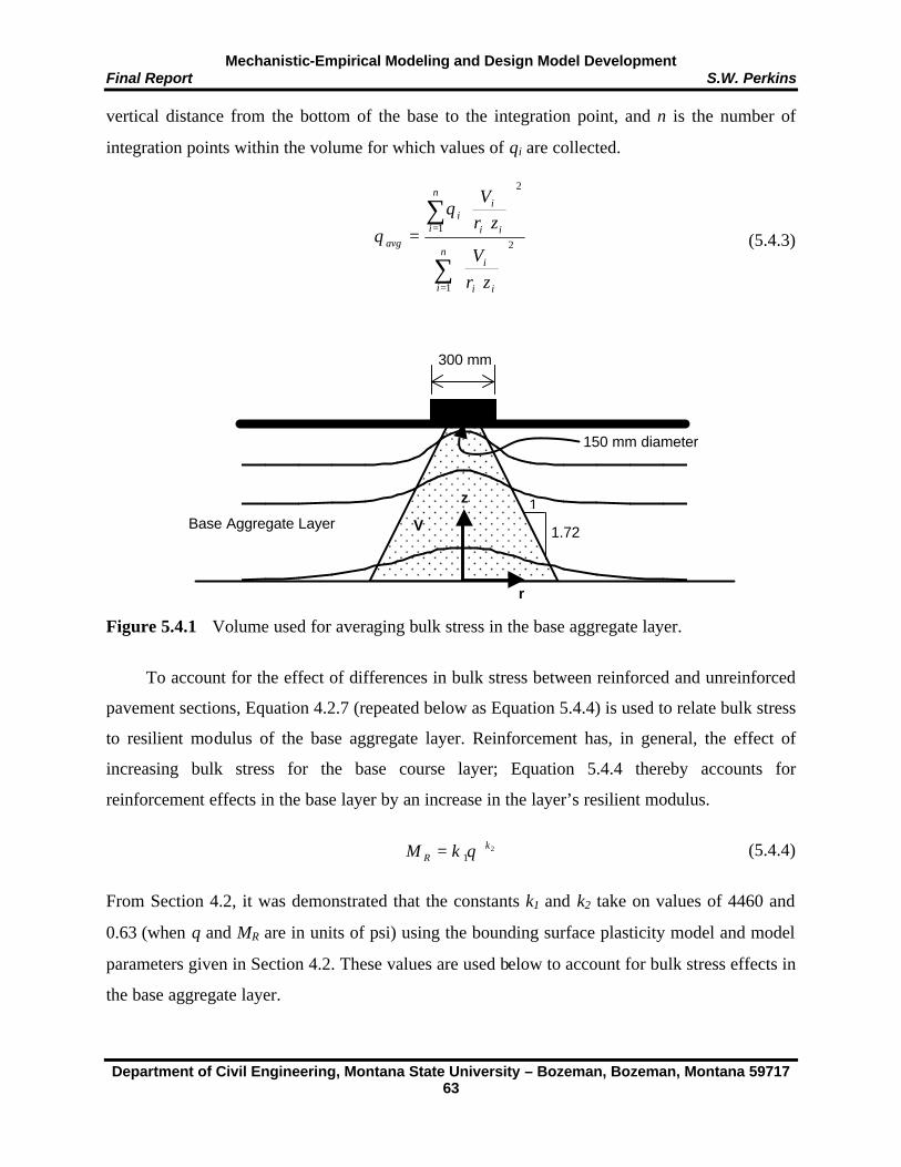
Mechanistic-Empirical Modeling and Design Model Development Final Report S.W. Perkins
Department of Civil Engineering, Montana State University – Bozeman, Bozeman, Montana 59717 63
21
kR kM θ=
vertical distance from the bottom of the base to the integration point, and n is the number of
integration points within the volume for which values of θi are collected.
(5.4.3)
Figure 5.4.1 Volume used for averaging bulk stress in the base aggregate layer.
To account for the effect of differences in bulk stress between reinforced and unreinforced
pavement sections, Equation 4.2.7 (repeated below as Equation 5.4.4) is used to relate bulk stress
to resilient modulus of the base aggregate layer. Reinforcement has, in general, the effect of
increasing bulk stress for the base course layer; Equation 5.4.4 thereby accounts for
reinforcement effects in the base layer by an increase in the layer’s resilient modulus.
(5.4.4)
From Section 4.2, it was demonstrated that the constants k1 and k2 take on values of 4460 and
0.63 (when θ and MR are in units of psi) using the bounding surface plasticity model and model
parameters given in Section 4.2. These values are used below to account for bulk stress effects in
the base aggregate layer.
∑
∑
=
=
=n
i ii
i
n
i ii
ii
avg
zrV
zrV
1
2
1
2
θθ
1
1.72
300 mm
150 mm diameter
Base Aggregate Layer
r
z
V
Mechanistic-Empirical Modeling and Design Model Development Final Report S.W. Perkins
Department of Civil Engineering, Montana State University – Bozeman, Bozeman, Montana 59717 64
22211 mDaDaSN +=
( ) 977.0log249.02 −= RMa
The 1993 AASHTO pavement design equation (Equation 5.4.5) is used to calculate the
number of ESAL’s (W18) for a reinforced and an unreinforced pavement section for which θ has
been individually evaluated and MR determined from Equation 5.4.4.
(5.4.5)
In Equation 5.4.5, ZR is the standard normal deviate, So is the combined standard error and ∆PSI
is the loss of design serviceability. Values of ZR, So ∆PSI have been taken as constants for all
pavement geometries analyzed and have been given values of -1.645, 0.35 and 1.9, respectively,
where the value of ZR used corresponds to a reliability of 95 %. In Equation 5.4.5, MS is the
effective roadbed (subgrade) resilient modulus where values are assigned according to Equation
4.2.9 for the different subgrades modeled. The structural number (SN) in Equation 5.4.5 is given
by
(5.4.6)
where a1 and a2 are the layer coefficients of the asphalt concrete and base aggregate layers,
respectively, D1 and D2 are the thicknesses of the AC and base layers, respectively, and m2 is the
drainage coefficient of the base layer. The layer coefficient a1 is taken as 0.4, which was shown
in Section 4.1 to be comparable with the modulus values used for this layer in the finite element
models. The drainage coefficient is taken as 1.0. The base layer coefficient, a2, is given in terms
of resilient modulus by Equation 5.4.7 (AASHTO, 1993).
(5.4.7)
Based on a particular pavement geometry, defining values of D1 and D2, and a value for MS, the
finite element model is analyzed for the reinforced and unreinforced case with values of mean
stress extracted from each. Equations 5.4.5 – 5.4.7 are used to evaluate W18 for the reinforced
and unreinforced pavements. The ratio of W18 for the reinforced and unreinforced pavements
( )
( )
−+
++
−∆
+−++= 07.8)log(32.2
11094
4.0
5.12.4log
2.01log36.9^10
19.5
18 SoR M
SN
PSI
SNSZW

Mechanistic-Empirical Modeling and Design Model Development Final Report S.W. Perkins
Department of Civil Engineering, Montana State University – Bozeman, Bozeman, Montana 59717 65
U
RB W
WTBR
−
−=18
18
SBT TBRTBRTBR ×=
then defines a TBR for reinforcement of the base, with this TBR viewed as a partial TBR and
written as:
(5.4.8)
The two partial TBR’s need to be combined together to define a total TBR for the pavement.
An explicit expression between partial and total TBR that involves only load cycle and rut depth
parameters is not possible without making significant assumptions regarding the shape of the
surface deformation versus load cycle curves. It is possible, however, to compute a total TBR
through the use of the AASHTO 1993 pavement design equation (Equation 5.4.5). This is done
by using Equation 5.4.5 to determine an increased resilient modulus for the subgrade that
produces a TBR for the subgrade as defined from Equation 5.4.2, while the base layer
coefficients are equal for reinforced and unreinforced cases. Base and subgrade effects are then
combined together in Equation 5.4.5 by keeping the higher resilient modulus for the subgrade
and including the mean stress effect of the higher resilient modulus for the base layer. Because of
the log nature of Equation 5.4.5 and the effect of increases in resilient modulus of the subgrade
and increases in structural number due to an increase in base layer modulus, this approach is the
same as defining the total TBR from the product of the partial TBR’s (Equation 5.4.9).
(5.4.9)
The use of Equation 5.4.9 is conservative in comparison to that which has been observed from
test sections described in Section 3. Examination of Table 3.2.1 shows that the use of Equation
5.4.9 to compute TBRT from TBRB and TBRS yields values that are in all cases less than the
values of TBRT observed directly from test section results. It should be noted that all TBR’s
discussed above pertain to values for the condition where BCR = 0.
6.0 PARAMETRIC STUDY AND RESULTS
Material presented in Section 2.1 indicated that current research work shows that the benefit
derived from geosynthetic reinforcement is strongly dependent on design parameters associated
with the pavement system and on material properties and characteristics associated with the
geosynthetic. Reinforcement benefit is generally seen to be dependent on the strength and/or
Mechanistic-Empirical Modeling and Design Model Development Final Report S.W. Perkins
Department of Civil Engineering, Montana State University – Bozeman, Bozeman, Montana 59717 66
stiffness of the subgrade layer. Reinforcement benefit generally increases as subgrade CBR
decreases. Reinforcement benefit is generally thought to be negligible above a subgrade CBR of
8. Reinforcement benefit is also dependent on the thickness of the structural section of the
pavement, including the AC and base aggregate. For very thin sections with low structural
numbers, base reinforcement does not appear to offer significant benefit. As structural sections
become very thick, reinforcement benefit is seen to diminish. As described in Section 5, a finite
element model simulating perfect reinforcement was created to examine the effect of these
pavement variables (AC and base thickness, and subgrade properties) on reinforcement benefit.
Results from this model involving cases where these parameters are varied are described in
Section 6.1.
Material presented in Section 2.1 indicated that tensile modulus of the geosynthetic is an
important design parameter, suggesting also that the ratio of modulus in the weak and strong
directions of the material should be important. The definition of other material properties related
to the type and structure of the geosynthetic that can be used directly in a structural analysis of a
reinforced pavement is not as clear. Material presented in Section 4.3 indicated that certain
properties within the context of an anisotropic linear elastic model for the geosynthetic could be
varied and shown to affect the apparent or effective stiffness of the material under biaxial
loading. These parameters (Poisson’s ratio and shear modulus) are shown here and in Section 7
to have a seconday influence on reinforcement benefit.
6.1 Variation of Parameters for Perfect Reinforced Models
All models examined under the parametric study used the same properties for the asphalt
concrete and base aggregate layer as described in Sections 4.1 and 4.2, respectively. Material
parameters for the asphalt concrete and base aggregate were given in Tables 4.1.2 and 4.2.2,
respectively. As discussed previously, the values of modulus used for the asphalt concrete
approximate a material with a layer coefficient of 0.4 (AASHTO, 1993). The resilient modulus
values that were inferred from the use of the material model for the base aggregate represented
an aggregate in a damp state with a layer coefficient ranging from 0.08 to 0.12.
For the perfect reinforced models, AC thickness, base thickness and subgrade properties
were varied. The values of AC thickness and base thickness used, along with corresponding case
names, are given in Table 6.1.1 and 6.1.2.
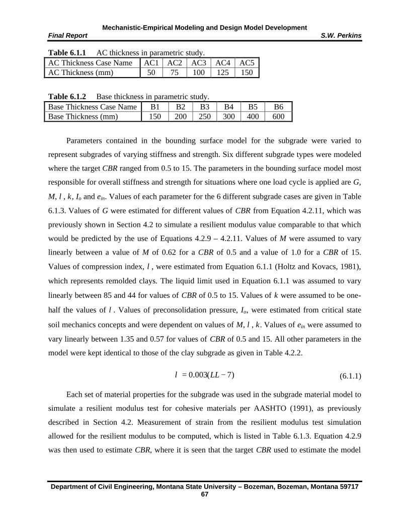
Mechanistic-Empirical Modeling and Design Model Development Final Report S.W. Perkins
Department of Civil Engineering, Montana State University – Bozeman, Bozeman, Montana 59717 67
)7(003.0 −= LLλ
Table 6.1.1 AC thickness in parametric study. AC Thickness Case Name AC1 AC2 AC3 AC4 AC5 AC Thickness (mm) 50 75 100 125 150
Table 6.1.2 Base thickness in parametric study. Base Thickness Case Name B1 B2 B3 B4 B5 B6 Base Thickness (mm) 150 200 250 300 400 600
Parameters contained in the bounding surface model for the subgrade were varied to
represent subgrades of varying stiffness and strength. Six different subgrade types were modeled
where the target CBR ranged from 0.5 to 15. The parameters in the bounding surface model most
responsible for overall stiffness and strength for situations where one load cycle is applied are G,
M, λ, κ, Io and ein. Values of each parameter for the 6 different subgrade cases are given in Table
6.1.3. Values of G were estimated for different values of CBR from Equation 4.2.11, which was
previously shown in Section 4.2 to simulate a resilient modulus value comparable to that which
would be predicted by the use of Equations 4.2.9 – 4.2.11. Values of M were assumed to vary
linearly between a value of M of 0.62 for a CBR of 0.5 and a value of 1.0 for a CBR of 15.
Values of compression index, λ, were estimated from Equation 6.1.1 (Holtz and Kovacs, 1981),
which represents remolded clays. The liquid limit used in Equation 6.1.1 was assumed to vary
linearly between 85 and 44 for values of CBR of 0.5 to 15. Values of κ were assumed to be one-
half the values of λ. Values of preconsolidation pressure, Io, were estimated from critical state
soil mechanics concepts and were dependent on values of M, λ, κ. Values of ein were assumed to
vary linearly between 1.35 and 0.57 for values of CBR of 0.5 and 15. All other parameters in the
model were kept identical to those of the clay subgrade as given in Table 4.2.2.
(6.1.1)
Each set of material properties for the subgrade was used in the subgrade material model to
simulate a resilient modulus test for cohesive materials per AASHTO (1991), as previously
described in Section 4.2. Measurement of strain from the resilient modulus test simulation
allowed for the resilient modulus to be computed, which is listed in Table 6.1.3. Equation 4.2.9
was then used to estimate CBR, where it is seen that the target CBR used to estimate the model
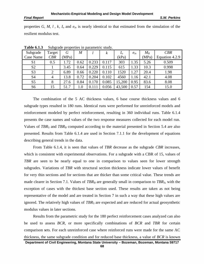
Mechanistic-Empirical Modeling and Design Model Development Final Report S.W. Perkins
Department of Civil Engineering, Montana State University – Bozeman, Bozeman, Montana 59717 68
properties G, M, λ, κ, Io and ein is nearly identical to that estimated from the simulation of the
resilient modulus test.
Table 6.1.3 Subgrade properties in parametric study. Subgrade
Case Name Target CBR
G (MPa)
M λ κ Io (kPa)
ein MR (MPa)
CBR Equation 4.2.9
S1 0.5 1.72 0.62 0.233 0.117 303 1.35 5.26 0.509 S2 1 3.45 0.64 0.229 0.115 615 1.33 10.3 0.998 S3 2 6.89 0.66 0.220 0.110 1520 1.27 20.4 1.98 S4 4 13.8 0.72 0.204 0.102 4560 1.16 42.1 4.08 S5 8 27.6 0.84 0.170 0.085 15,200 0.95 83.6 8.08 S6 15 51.7 1.0 0.111 0.056 43,500 0.57 154 15.0
The combination of the 5 AC thickness values, 6 base course thickness values and 6
subgrade types resulted in 180 runs. Identical runs were performed for unreinforced models and
reinforcement modeled by perfect reinforcement, resulting in 360 individual runs. Table 6.1.4
presents the case names and values of the two response measures collected for each model run.
Values of TBRS and TBRB computed according to the material presented in Section 5.4 are also
presented. Results from Table 6.1.4 are used in Section 7.1.1 for the development of equations
describing general trends in the data.
From Table 6.1.4, it is seen that values of TBR decrease as the subgrade CBR increases,
which is consistent with experimental observations. For a subgrade with a CBR of 15, values of
TBR are seen to be nearly equal to one in comparison to values seen for lower strength
subgrades. Variations of TBR with structural section thickness indicate lower values of benefit
for very thin sections and for sections that are thicker than some critical value. These trends are
made clearer in Section 7.1. Values of TBRB are generally small in comparison to TBRS, with the
exception of cases with the thickest base section used. These results are taken as not being
representative of the model and are treated in Section 7 in such a way that these high values are
ignored. The relatively high values of TBRS are expected and are reduced for actual geosynthetic
modulus values in later sections.
Results from the parametric study for the 180 perfect reinforcement cases analyzed can also
be used to assess BCR, or more specifically combinations of BCR and TBR for certain
comparison sets. For each unreinforced case where reinforced runs were made for the same AC
thickness, the same subgrade condition and for reduced base thickness, a value of BCR is known

Mechanistic-Empirical Modeling and Design Model Development Final Report S.W. Perkins
Department of Civil Engineering, Montana State University – Bozeman, Bozeman, Montana 59717 69
or presumed from the established base thickness of the unreinforced and reinforced models. For
instance, if case AC1-B6-S1 for an unreinforced pavement is compared to AC1-B5-S1 for a
reinforced case, a BCR of 33 % is presumed as the two models are established. From the 360
model runs, 75 sets of unreinforced and reinforced comparison runs, where a BCR was
presumed, were available for each of the 6 subgrade conditions, giving 450 comparisons for the
6 subgrade conditions. The response measures of vertical subgrade strain and bulk stress in the
base aggregate were compared between these comparison runs to assess TBRS and TBRB. Values
greater than one indicate a remaining TBR for the assumed BCR. Values less than one indicate
that the assumed BCR resulted in a reduction of life of the reinforced pavement as compared to
the reinforced section.
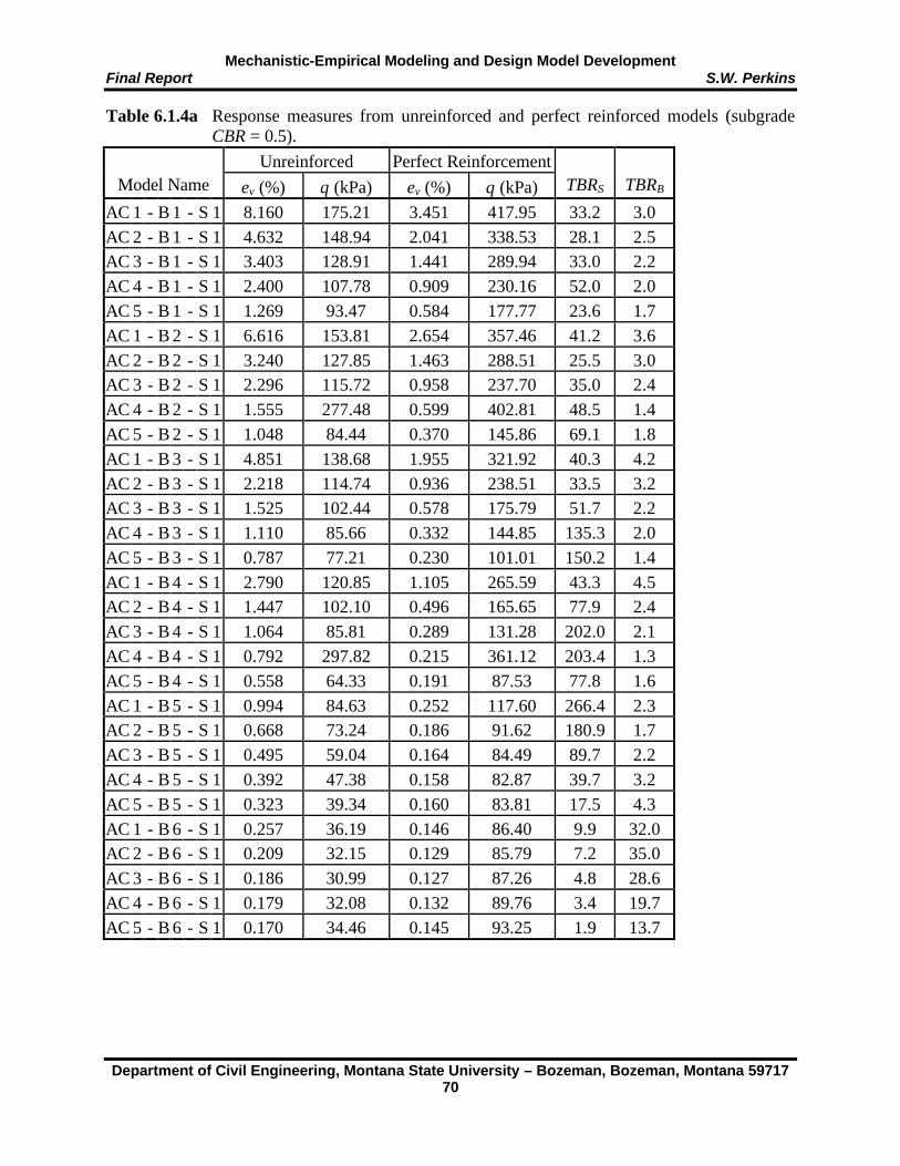
Mechanistic-Empirical Modeling and Design Model Development Final Report S.W. Perkins
Department of Civil Engineering, Montana State University – Bozeman, Bozeman, Montana 59717 70
Table 6.1.4a Response measures from unreinforced and perfect reinforced models (subgrade CBR = 0.5).
Unreinforced Perfect Reinforcement Model Name εv (%) θ (kPa) εv (%) θ (kPa) TBRS TBRB
AC 1 - B 1 - S 1 8.160 175.21 3.451 417.95 33.2 3.0 AC 2 - B 1 - S 1 4.632 148.94 2.041 338.53 28.1 2.5 AC 3 - B 1 - S 1 3.403 128.91 1.441 289.94 33.0 2.2 AC 4 - B 1 - S 1 2.400 107.78 0.909 230.16 52.0 2.0 AC 5 - B 1 - S 1 1.269 93.47 0.584 177.77 23.6 1.7 AC 1 - B 2 - S 1 6.616 153.81 2.654 357.46 41.2 3.6 AC 2 - B 2 - S 1 3.240 127.85 1.463 288.51 25.5 3.0 AC 3 - B 2 - S 1 2.296 115.72 0.958 237.70 35.0 2.4 AC 4 - B 2 - S 1 1.555 277.48 0.599 402.81 48.5 1.4 AC 5 - B 2 - S 1 1.048 84.44 0.370 145.86 69.1 1.8 AC 1 - B 3 - S 1 4.851 138.68 1.955 321.92 40.3 4.2 AC 2 - B 3 - S 1 2.218 114.74 0.936 238.51 33.5 3.2 AC 3 - B 3 - S 1 1.525 102.44 0.578 175.79 51.7 2.2 AC 4 - B 3 - S 1 1.110 85.66 0.332 144.85 135.3 2.0 AC 5 - B 3 - S 1 0.787 77.21 0.230 101.01 150.2 1.4 AC 1 - B 4 - S 1 2.790 120.85 1.105 265.59 43.3 4.5 AC 2 - B 4 - S 1 1.447 102.10 0.496 165.65 77.9 2.4 AC 3 - B 4 - S 1 1.064 85.81 0.289 131.28 202.0 2.1 AC 4 - B 4 - S 1 0.792 297.82 0.215 361.12 203.4 1.3 AC 5 - B 4 - S 1 0.558 64.33 0.191 87.53 77.8 1.6 AC 1 - B 5 - S 1 0.994 84.63 0.252 117.60 266.4 2.3 AC 2 - B 5 - S 1 0.668 73.24 0.186 91.62 180.9 1.7 AC 3 - B 5 - S 1 0.495 59.04 0.164 84.49 89.7 2.2 AC 4 - B 5 - S 1 0.392 47.38 0.158 82.87 39.7 3.2 AC 5 - B 5 - S 1 0.323 39.34 0.160 83.81 17.5 4.3 AC 1 - B 6 - S 1 0.257 36.19 0.146 86.40 9.9 32.0 AC 2 - B 6 - S 1 0.209 32.15 0.129 85.79 7.2 35.0 AC 3 - B 6 - S 1 0.186 30.99 0.127 87.26 4.8 28.6 AC 4 - B 6 - S 1 0.179 32.08 0.132 89.76 3.4 19.7 AC 5 - B 6 - S 1 0.170 34.46 0.145 93.25 1.9 13.7

Mechanistic-Empirical Modeling and Design Model Development Final Report S.W. Perkins
Department of Civil Engineering, Montana State University – Bozeman, Bozeman, Montana 59717 71
Table 6.1.4b Response measures from unreinforced and perfect reinforced models (subgrade CBR = 1).
Unreinforced Perfect Reinforcement Model Name εv (%) θ (kPa) εv (%) θ (kPa) TBRS TBRB
AC 1 - B 1 - S 2 4.882 203.77 2.501 487.38 15.2 2.9 AC 2 - B 1 - S 2 2.809 184.22 1.601 376.17 9.9 2.2 AC 3 - B 1 - S 2 2.247 165.82 1.210 325.56 12.4 1.9 AC 4 - B 1 - S 2 1.705 139.48 0.808 272.18 20.8 1.8 AC 5 - B 1 - S 2 1.113 119.29 0.528 216.65 20.8 1.6 AC 1 - B 2 - S 2 3.545 193.11 1.900 399.06 12.7 2.9 AC 2 - B 2 - S 2 2.145 162.74 1.182 315.78 11.3 2.4 AC 3 - B 2 - S 2 1.681 143.35 0.828 267.71 17.9 2.1 AC 4 - B 2 - S 2 1.265 312.76 0.517 431.76 38.2 1.4 AC 5 - B 2 - S 2 0.896 101.72 0.319 160.42 66.5 1.6 AC 1 - B 3 - S 2 2.423 168.87 1.324 329.25 11.7 3.0 AC 2 - B 3 - S 2 1.592 140.82 0.758 264.61 20.5 2.6 AC 3 - B 3 - S 2 1.217 120.29 0.467 202.28 49.3 2.1 AC 4 - B 3 - S 2 0.920 100.68 0.291 150.84 107.6 1.7 AC 5 - B 3 - S 2 0.646 89.02 0.220 107.56 80.2 1.3 AC 1 - B 4 - S 2 1.659 143.46 0.793 271.75 20.2 3.3 AC 2 - B 4 - S 2 1.136 116.53 0.394 179.42 74.7 2.2 AC 3 - B 4 - S 2 0.857 94.70 0.260 134.76 127.9 1.8 AC 4 - B 4 - S 2 0.641 308.76 0.205 360.74 104.3 1.2 AC 5 - B 4 - S 2 0.455 69.83 0.183 94.05 41.0 1.5 AC 1 - B 5 - S 2 0.771 90.50 0.226 118.37 148.3 2.0 AC 2 - B 5 - S 2 0.525 78.15 0.177 96.55 84.1 1.7 AC 3 - B 5 - S 2 0.396 63.54 0.156 89.47 44.6 2.1 AC 4 - B 5 - S 2 0.319 52.61 0.148 87.54 22.8 2.8 AC 5 - B 5 - S 2 0.268 45.03 0.145 88.06 12.0 3.6 AC 1 - B 6 - S 2 0.207 40.06 0.126 89.06 7.7 21.3 AC 2 - B 6 - S 2 0.173 36.15 0.114 88.73 5.4 22.6 AC 3 - B 6 - S 2 0.156 35.12 0.112 90.11 3.8 18.9 AC 4 - B 6 - S 2 0.149 36.86 0.114 92.30 3.0 13.1 AC 5 - B 6 - S 2 0.143 39.93 0.119 95.17 2.1 9.3
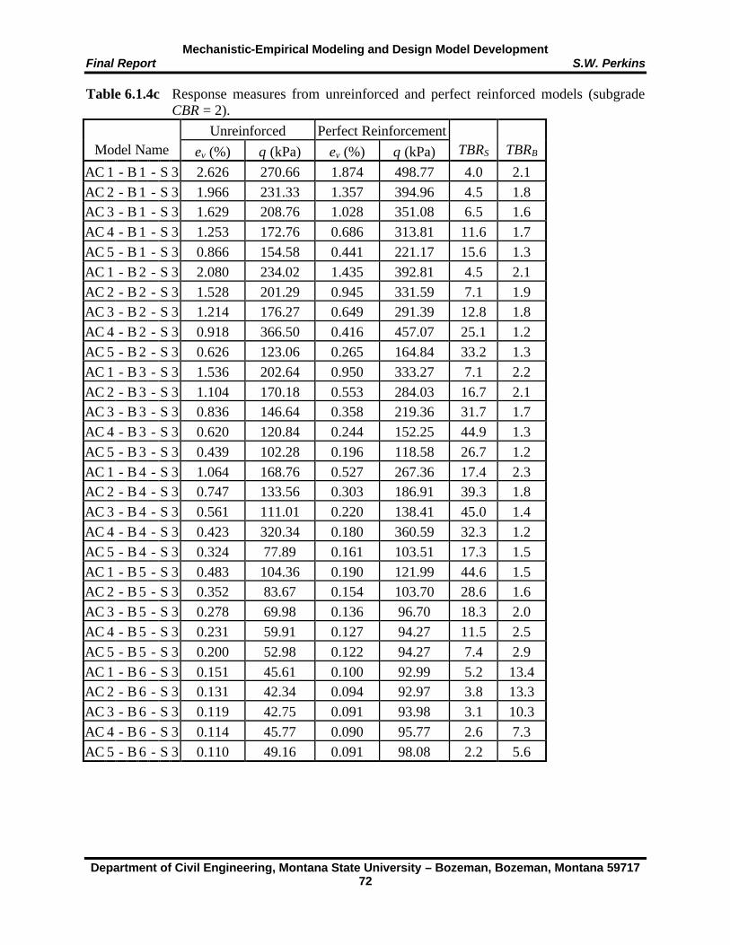
Mechanistic-Empirical Modeling and Design Model Development Final Report S.W. Perkins
Department of Civil Engineering, Montana State University – Bozeman, Bozeman, Montana 59717 72
Table 6.1.4c Response measures from unreinforced and perfect reinforced models (subgrade CBR = 2).
Unreinforced Perfect Reinforcement Model Name εv (%) θ (kPa) εv (%) θ (kPa) TBRS TBRB
AC 1 - B 1 - S 3 2.626 270.66 1.874 498.77 4.0 2.1 AC 2 - B 1 - S 3 1.966 231.33 1.357 394.96 4.5 1.8 AC 3 - B 1 - S 3 1.629 208.76 1.028 351.08 6.5 1.6 AC 4 - B 1 - S 3 1.253 172.76 0.686 313.81 11.6 1.7 AC 5 - B 1 - S 3 0.866 154.58 0.441 221.17 15.6 1.3 AC 1 - B 2 - S 3 2.080 234.02 1.435 392.81 4.5 2.1 AC 2 - B 2 - S 3 1.528 201.29 0.945 331.59 7.1 1.9 AC 3 - B 2 - S 3 1.214 176.27 0.649 291.39 12.8 1.8 AC 4 - B 2 - S 3 0.918 366.50 0.416 457.07 25.1 1.2 AC 5 - B 2 - S 3 0.626 123.06 0.265 164.84 33.2 1.3 AC 1 - B 3 - S 3 1.536 202.64 0.950 333.27 7.1 2.2 AC 2 - B 3 - S 3 1.104 170.18 0.553 284.03 16.7 2.1 AC 3 - B 3 - S 3 0.836 146.64 0.358 219.36 31.7 1.7 AC 4 - B 3 - S 3 0.620 120.84 0.244 152.25 44.9 1.3 AC 5 - B 3 - S 3 0.439 102.28 0.196 118.58 26.7 1.2 AC 1 - B 4 - S 3 1.064 168.76 0.527 267.36 17.4 2.3 AC 2 - B 4 - S 3 0.747 133.56 0.303 186.91 39.3 1.8 AC 3 - B 4 - S 3 0.561 111.01 0.220 138.41 45.0 1.4 AC 4 - B 4 - S 3 0.423 320.34 0.180 360.59 32.3 1.2 AC 5 - B 4 - S 3 0.324 77.89 0.161 103.51 17.3 1.5 AC 1 - B 5 - S 3 0.483 104.36 0.190 121.99 44.6 1.5 AC 2 - B 5 - S 3 0.352 83.67 0.154 103.70 28.6 1.6 AC 3 - B 5 - S 3 0.278 69.98 0.136 96.70 18.3 2.0 AC 4 - B 5 - S 3 0.231 59.91 0.127 94.27 11.5 2.5 AC 5 - B 5 - S 3 0.200 52.98 0.122 94.27 7.4 2.9 AC 1 - B 6 - S 3 0.151 45.61 0.100 92.99 5.2 13.4 AC 2 - B 6 - S 3 0.131 42.34 0.094 92.97 3.8 13.3 AC 3 - B 6 - S 3 0.119 42.75 0.091 93.98 3.1 10.3 AC 4 - B 6 - S 3 0.114 45.77 0.090 95.77 2.6 7.3 AC 5 - B 6 - S 3 0.110 49.16 0.091 98.08 2.2 5.6
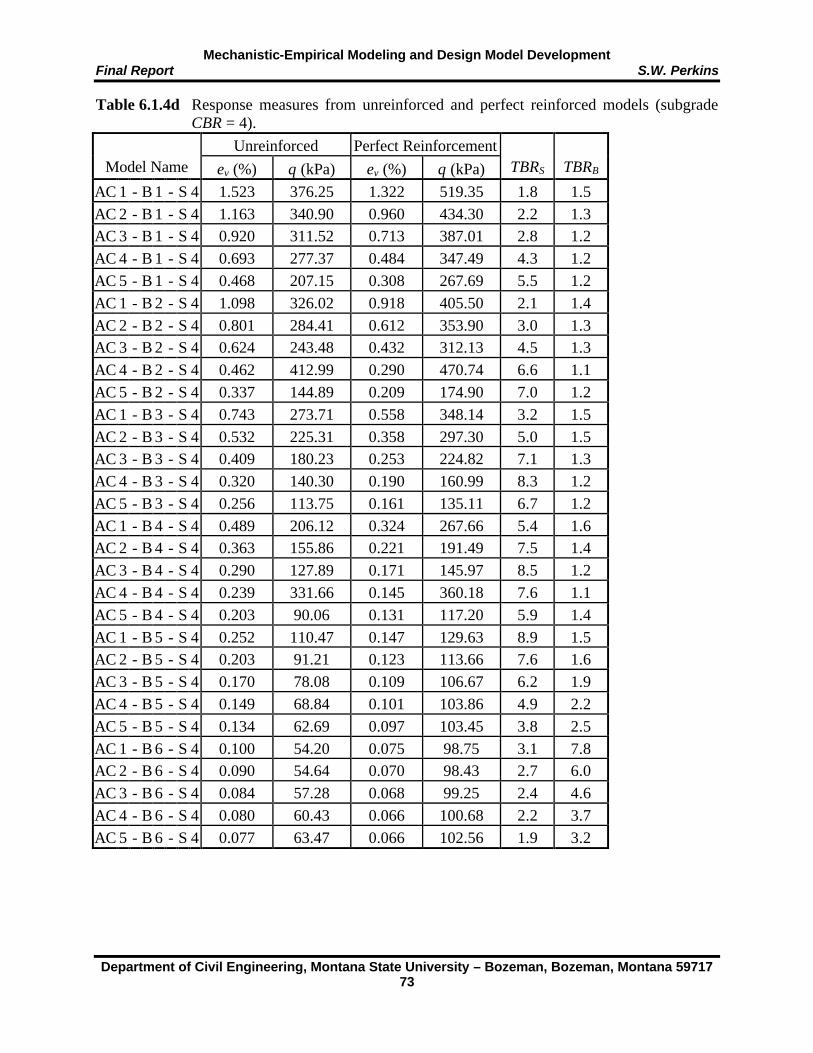
Mechanistic-Empirical Modeling and Design Model Development Final Report S.W. Perkins
Department of Civil Engineering, Montana State University – Bozeman, Bozeman, Montana 59717 73
Table 6.1.4d Response measures from unreinforced and perfect reinforced models (subgrade CBR = 4).
Unreinforced Perfect Reinforcement Model Name εv (%) θ (kPa) εv (%) θ (kPa) TBRS TBRB
AC 1 - B 1 - S 4 1.523 376.25 1.322 519.35 1.8 1.5 AC 2 - B 1 - S 4 1.163 340.90 0.960 434.30 2.2 1.3 AC 3 - B 1 - S 4 0.920 311.52 0.713 387.01 2.8 1.2 AC 4 - B 1 - S 4 0.693 277.37 0.484 347.49 4.3 1.2 AC 5 - B 1 - S 4 0.468 207.15 0.308 267.69 5.5 1.2 AC 1 - B 2 - S 4 1.098 326.02 0.918 405.50 2.1 1.4 AC 2 - B 2 - S 4 0.801 284.41 0.612 353.90 3.0 1.3 AC 3 - B 2 - S 4 0.624 243.48 0.432 312.13 4.5 1.3 AC 4 - B 2 - S 4 0.462 412.99 0.290 470.74 6.6 1.1 AC 5 - B 2 - S 4 0.337 144.89 0.209 174.90 7.0 1.2 AC 1 - B 3 - S 4 0.743 273.71 0.558 348.14 3.2 1.5 AC 2 - B 3 - S 4 0.532 225.31 0.358 297.30 5.0 1.5 AC 3 - B 3 - S 4 0.409 180.23 0.253 224.82 7.1 1.3 AC 4 - B 3 - S 4 0.320 140.30 0.190 160.99 8.3 1.2 AC 5 - B 3 - S 4 0.256 113.75 0.161 135.11 6.7 1.2 AC 1 - B 4 - S 4 0.489 206.12 0.324 267.66 5.4 1.6 AC 2 - B 4 - S 4 0.363 155.86 0.221 191.49 7.5 1.4 AC 3 - B 4 - S 4 0.290 127.89 0.171 145.97 8.5 1.2 AC 4 - B 4 - S 4 0.239 331.66 0.145 360.18 7.6 1.1 AC 5 - B 4 - S 4 0.203 90.06 0.131 117.20 5.9 1.4 AC 1 - B 5 - S 4 0.252 110.47 0.147 129.63 8.9 1.5 AC 2 - B 5 - S 4 0.203 91.21 0.123 113.66 7.6 1.6 AC 3 - B 5 - S 4 0.170 78.08 0.109 106.67 6.2 1.9 AC 4 - B 5 - S 4 0.149 68.84 0.101 103.86 4.9 2.2 AC 5 - B 5 - S 4 0.134 62.69 0.097 103.45 3.8 2.5 AC 1 - B 6 - S 4 0.100 54.20 0.075 98.75 3.1 7.8 AC 2 - B 6 - S 4 0.090 54.64 0.070 98.43 2.7 6.0 AC 3 - B 6 - S 4 0.084 57.28 0.068 99.25 2.4 4.6 AC 4 - B 6 - S 4 0.080 60.43 0.066 100.68 2.2 3.7 AC 5 - B 6 - S 4 0.077 63.47 0.066 102.56 1.9 3.2

Mechanistic-Empirical Modeling and Design Model Development Final Report S.W. Perkins
Department of Civil Engineering, Montana State University – Bozeman, Bozeman, Montana 59717 74
Table 6.1.4e Response measures from unreinforced and perfect reinforced models (subgrade CBR = 8).
Unreinforced Perfect Reinforcement Model Name εv (%) θ (kPa) εv (%) θ (kPa) TBRS TBRB
AC 1 - B 1 - S 5 0.661 563.93 0.675 574.42 0.9 1.0 AC 2 - B 1 - S 5 0.531 491.42 0.531 495.91 1.0 1.0 AC 3 - B 1 - S 5 0.423 420.18 0.414 426.73 1.1 1.0 AC 4 - B 1 - S 5 0.326 340.51 0.302 368.89 1.4 1.1 AC 5 - B 1 - S 5 0.251 242.63 0.214 288.44 1.9 1.1 AC 1 - B 2 - S 5 0.468 436.83 0.476 439.19 0.9 1.0 AC 2 - B 2 - S 5 0.365 367.84 0.358 380.26 1.1 1.0 AC 3 - B 2 - S 5 0.294 291.22 0.269 324.40 1.4 1.1 AC 4 - B 2 - S 5 0.232 441.35 0.196 472.33 2.0 1.1 AC 5 - B 2 - S 5 0.192 166.31 0.156 201.33 2.3 1.2 AC 1 - B 3 - S 5 0.325 333.76 0.316 356.81 1.1 1.1 AC 2 - B 3 - S 5 0.256 262.45 0.228 301.41 1.6 1.2 AC 3 - B 3 - S 5 0.206 195.28 0.171 227.90 2.1 1.2 AC 4 - B 3 - S 5 0.173 151.47 0.137 176.86 2.5 1.2 AC 5 - B 3 - S 5 0.152 128.56 0.121 157.25 2.5 1.3 AC 1 - B 4 - S 5 0.232 225.65 0.203 267.13 1.7 1.3 AC 2 - B 4 - S 5 0.186 168.13 0.152 197.63 2.3 1.3 AC 3 - B 4 - S 5 0.156 134.78 0.123 158.87 2.6 1.3 AC 4 - B 4 - S 5 0.136 342.53 0.108 360.25 2.6 1.1 AC 5 - B 4 - S 5 0.123 103.26 0.100 135.81 2.4 1.5 AC 1 - B 5 - S 5 0.135 115.63 0.105 140.56 2.8 1.6 AC 2 - B 5 - S 5 0.115 98.54 0.090 126.62 2.7 1.7 AC 3 - B 5 - S 5 0.101 86.95 0.081 120.00 2.5 1.9 AC 4 - B 5 - S 5 0.091 80.19 0.076 117.22 2.2 2.0 AC 5 - B 5 - S 5 0.085 78.41 0.072 116.66 2.0 2.0 AC 1 - B 6 - S 5 0.063 73.83 0.054 106.82 1.9 3.2 AC 2 - B 6 - S 5 0.058 75.50 0.051 106.28 1.8 2.6 AC 3 - B 6 - S 5 0.055 77.76 0.048 106.75 1.7 2.3 AC 4 - B 6 - S 5 0.053 80.22 0.047 107.82 1.6 2.1 AC 5 - B 6 - S 5 0.051 82.54 0.046 109.28 1.6 1.9
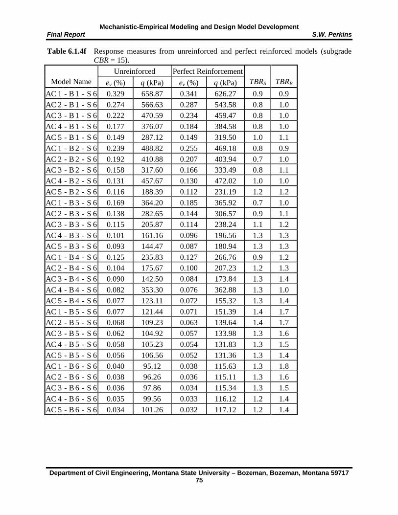
Mechanistic-Empirical Modeling and Design Model Development Final Report S.W. Perkins
Department of Civil Engineering, Montana State University – Bozeman, Bozeman, Montana 59717 75
Table 6.1.4f Response measures from unreinforced and perfect reinforced models (subgrade CBR = 15).
Unreinforced Perfect Reinforcement Model Name εv (%) θ (kPa) εv (%) θ (kPa) TBRS TBRB
AC 1 - B 1 - S 6 0.329 658.87 0.341 626.27 0.9 0.9 AC 2 - B 1 - S 6 0.274 566.63 0.287 543.58 0.8 1.0 AC 3 - B 1 - S 6 0.222 470.59 0.234 459.47 0.8 1.0 AC 4 - B 1 - S 6 0.177 376.07 0.184 384.58 0.8 1.0 AC 5 - B 1 - S 6 0.149 287.12 0.149 319.50 1.0 1.1 AC 1 - B 2 - S 6 0.239 488.82 0.255 469.18 0.8 0.9 AC 2 - B 2 - S 6 0.192 410.88 0.207 403.94 0.7 1.0 AC 3 - B 2 - S 6 0.158 317.60 0.166 333.49 0.8 1.1 AC 4 - B 2 - S 6 0.131 457.67 0.130 472.02 1.0 1.0 AC 5 - B 2 - S 6 0.116 188.39 0.112 231.19 1.2 1.2 AC 1 - B 3 - S 6 0.169 364.20 0.185 365.92 0.7 1.0 AC 2 - B 3 - S 6 0.138 282.65 0.144 306.57 0.9 1.1 AC 3 - B 3 - S 6 0.115 205.87 0.114 238.24 1.1 1.2 AC 4 - B 3 - S 6 0.101 161.16 0.096 196.56 1.3 1.3 AC 5 - B 3 - S 6 0.093 144.47 0.087 180.94 1.3 1.3 AC 1 - B 4 - S 6 0.125 235.83 0.127 266.76 0.9 1.2 AC 2 - B 4 - S 6 0.104 175.67 0.100 207.23 1.2 1.3 AC 3 - B 4 - S 6 0.090 142.50 0.084 173.84 1.3 1.4 AC 4 - B 4 - S 6 0.082 353.30 0.076 362.88 1.3 1.0 AC 5 - B 4 - S 6 0.077 123.11 0.072 155.32 1.3 1.4 AC 1 - B 5 - S 6 0.077 121.44 0.071 151.39 1.4 1.7 AC 2 - B 5 - S 6 0.068 109.23 0.063 139.64 1.4 1.7 AC 3 - B 5 - S 6 0.062 104.92 0.057 133.98 1.3 1.6 AC 4 - B 5 - S 6 0.058 105.23 0.054 131.83 1.3 1.5 AC 5 - B 5 - S 6 0.056 106.56 0.052 131.36 1.3 1.4 AC 1 - B 6 - S 6 0.040 95.12 0.038 115.63 1.3 1.8 AC 2 - B 6 - S 6 0.038 96.26 0.036 115.11 1.3 1.6 AC 3 - B 6 - S 6 0.036 97.86 0.034 115.34 1.3 1.5 AC 4 - B 6 - S 6 0.035 99.56 0.033 116.12 1.2 1.4 AC 5 - B 6 - S 6 0.034 101.26 0.032 117.12 1.2 1.4

Mechanistic-Empirical Modeling and Design Model Development Final Report S.W. Perkins
Department of Civil Engineering, Montana State University – Bozeman, Bozeman, Montana 59717 76
6.2 Variation of Parameters for Geosynthetic Reinforced Models
Results shown in Table 6.1.4 for model cases simulating perfect reinforcement gave relatively
high values of TBR for many cases. Since these models simulate a geosynthetic with an infinite
tensile stiffness and an infinitely stiff contact shear interface between the geosynthetic and the
base aggregate, high values of TBR were expected. Model cases were analyzed in this way to
isolate the effects of AC and base aggregate thickness, and subgrade properties. As discussed in
Section 4.3, the anisotropic elastic model used for the geosynthetic allows for the variation of
certain properties that are related to physical material properties and possibly material
characteristics related to the structure of the geosynthetic. These properties are the in-plane
elastic modulus, the ratio between the elastic modulus in the strong and weak directions of the
material, Poisson’s ratio, and in-plane shear modulus.
The effect of modulus was first examined by using the finite element model described in
Section 5.3 with isotropic material properties used for the geosynthetic. Comparison of results to
those from similar cases with perfect reinforcement allowed for an assessment of the influence of
modulus on reinforcement benefit. Additional cases were created where an anisotropic model
was used to examine the effect of the ratio of the modulus in the strong and weak directions of
the material. Further cases were created to examine the effect of Poisson’s ratio and shear
modulus.
6.2.1 Parameters to Examine Effect of Reinforcement Modulus
The finite model described in Section 5.3 was used to examine the influence of the isotropic
value of elastic modulus of the geosynthetic on reinforcement benefit. The material model
described in Section 4.3 was used for the geosynthetic. All other material layers used the
material models previously described with specific properties as summarized below. The
material model for the geosynthetic was given elastic properties that represented an isotropic
material. In particular, the three elastic moduli were given the same value, the three Poisson’s
ratios were given the same value and the shear modulus was computed from the elastic modulus
and Poisson’s ratio as for an isotropic material. Five different values of geosynthetic isotropic
elastic modulus were used. Table 6.2.1 gives the values for each of the nine elastic constants
contained in the material model for the geosynthetic.

Mechanistic-Empirical Modeling and Design Model Development Final Report S.W. Perkins
Department of Civil Engineering, Montana State University – Bozeman, Bozeman, Montana 59717 77
Table 6.2.1 Parameters for geosynthetic material model to examine effect of reinforcement modulus.
Case Name
Exm (MPa)
Em
(MPa) En
(MPa) νxm-m νxm-n νm-n Gxm-m
(MPa) Gxm-n
(MPa) Gm-n
(MPa) GM1 400 400 400 0.5 0.5 0.5 133 133 133 GM2 1000 1000 1000 0.5 0.5 0.5 333 333 333 GM3 2000 2000 2000 0.5 0.5 0.5 667 667 667 GM4 4000 4000 4000 0.5 0.5 0.5 1333 1333 1333 GM5 8000 8000 8000 0.5 0.5 0.5 2667 2667 2667 Values of Poisson’s ratio were set equal to 0.5 since those values produce the stiffest
response of the material, as indicated in Section 4.3. The reduction of reinforcement benefit
produced by reducing Poisson’s ratio is examined in Section 6.2.3. Similarly, values of shear
modulus were set relatively high in order to produce maximum values of benefit. The effect of
reducing shear modulus is also examined in Section 6.2.3.
Ten pavement sections were analyzed with the case name for the AC and base thickness
given in Table 6.2.2. These cases were analyzed for the subgrade cases and geosynthetic material
property cases shown in Table 6.2.2, resulting in 250 additional model runs. The three groups of
pavement sections distinguished in Table 6.2.2 correspond to relatively thin, medium and thick
sections. As discussed in Section 7.2, results were run in these groups in order to provide a
means of modifying general trends in the data seen from the model runs for perfect
reinforcement described in Section 6.1 for the effect of reinforcement modulus.
Table 6.2.2 Pavement sections used to evaluate effect of reinforcement modulus. Pavement Section Subgrade Cases Geosynthetic Cases
AC1-B1 AC1-B2 AC2-B1 AC3-B4 AC4-B4 AC1-B5 AC2-B5 AC5-B5 AC3-B6 AC4-B6
S1, S2, S3, S4, S5 GM1, GM2, GM3, GM4, GM5

Mechanistic-Empirical Modeling and Design Model Development Final Report S.W. Perkins
Department of Civil Engineering, Montana State University – Bozeman, Bozeman, Montana 59717 78
6.2.2 Parameters to Examine Effect of Reinforcement Modulus Anisotropy
The finite element model described in Section 5.3 was used to examine the influence of direction
dependent geosynthetic elastic modulus values on reinforcement benefit. The material model
described in Section 4.3 was used for the geosynthetic. The model differed from that described in
Section 6.2.1 in that different values of elastic modulus were used in the machine and cross
machine directions. Values in the direction normal to the geosynthetic were also changed to
provide stability of the elastic matrix. All other material layers used the material models
previously described with specific properties as summarized below. Five different values of
geosynthetic modulus ratio, defined as the ratio of the minimum to maximum elastic modulus
values between the machine and cross machine directions, were used. These ratios were used for
two different values of maximum elastic modulus value. Table 6.2.3 gives the values for each of
the nine elastic constants contained in the material model for the geosynthetic.
Table 6.2.3 Parameters for geosynthetic material model to examine effect of reinforcement modulus anisotropy.
Case Name
Exm (MPa)
Em
(MPa) En
(MPa) Geosynthetic
Modulus Ratio (GMR)
νxm-m νxm-n νm-n Gxm-m
(MPa) Gxm-n
(MPa) Gm-n
(MPa)
GA1 400 400 400 1 0.5 0.5 0.5 133 133 133 GA2 400 300 300 0.75 0.5 0.5 0.5 133 133 133 GA3 400 200 200 0.5 0.5 0.5 0.5 133 133 133 GA4 400 100 100 0.25 0.5 0.5 0.5 133 133 133 GA5 400 40 40 0.1 0.5 0.5 0.5 133 133 133 GA6 8000 8000 8000 1 0.5 0.5 0.5 2667 2667 2667 GA7 800 6000 6000 0.75 0.5 0.5 0.5 2667 2667 2667 GA8 800 4000 4000 0.5 0.5 0.5 0.5 2667 2667 2667 GA9 800 2000 2000 0.25 0.5 0.5 0.5 2667 2667 2667 GA10 800 800 800 0.1 0.5 0.5 0.5 2667 2667 2667 Values of Poisson’s ratio were set equal to 0.5 since those values produce the stiffest
response of the material. The reduction of reinforcement benefit produced by reducing Poisson’s
ratio is examined in Section 6.2.3. Similarly, values of shear modulus were set high in order to
produce maximum values of benefit. The effect of reducing shear modulus is also examined in
Section 6.2.3.

Mechanistic-Empirical Modeling and Design Model Development Final Report S.W. Perkins
Department of Civil Engineering, Montana State University – Bozeman, Bozeman, Montana 59717 79
Three pavement sections were analyzed with the case name for the AC, base thickness and
subgrade CBR given in Table 6.2.4. These cases were analyzed for the geosynthetic material
property cases shown in Table 6.2.3, resulting in 30 additional model runs.
Table 6.2.4 Pavement sections used to evaluate effect of reinforcement modulus anisotropy. Pavement Section Geosynthetic Cases
AC2-B5-S1 AC1-B2-S3 AC5-B6-S5
GA1-GA10
6.2.3 Parameters to Examine Effect of Poisson’s Ratio and Shear Modulus
All finite element model cases previously examined used values for Poisson’s ratio and shear
modulus that would produce optimal values of reinforcement benefit with respect to these two
parameters. This was done such that the effects of reinforcement isotropic modulus and
reinforcement modulus anisotropy could be systematically accounted for. Additional finite
element model cases were created to examine the effect of reducing Poisson’s ratio and shear
modulus to their lowest possible values. Table 6.2.5 shows values of the elastic properties used
for the geosynthetic material model to examine the effect of reducing Poisson’s ratio and shear
modulus. These properties were used for each of the three pavement sections listed in Table
6.2.6, resulting in an additional 24 cases created to examine these effects.
Table 6.2.5 Parameters for geosynthetic material model to examine effect of reinforcement Poisson’s ratio and shear modulus.
Case Name
Exm (MPa)
Em
(MPa) En
(MPa) νxm-m νxm-n νm-n Gxm-m
(MPa) Gxm-n
(MPa) Gm-n
(MPa) GνG1 400 400 400 0.5 0.5 0.5 133 133 133 GνG2 8000 8000 8000 0.5 0.5 0.5 2667 2667 2667 GνG3 400 400 400 0 0 0 133 133 133 GνG4 8000 8000 8000 0 0 0 2667 2667 2667 GνG5 400 400 400 0.5 0.5 0.5 0 0 0 GνG6 8000 8000 8000 0.5 0.5 0.5 0 0 0 GνG7 400 400 400 0 0 0 0 0 0 GνG8 8000 8000 8000 0 0 0 0 0 0

Mechanistic-Empirical Modeling and Design Model Development Final Report S.W. Perkins
Department of Civil Engineering, Montana State University – Bozeman, Bozeman, Montana 59717 80
21 14.04.0 DDSN +=
Table 6.2.6 Pavement sections used to evaluate effect of reinforcement Poisson’s ratio and shear modulus.
Pavement Section Geosynthetic Cases AC2-B5-S1 AC1-B2-S3 AC5-B6-S5
GνG1- GνG8
All cases described in Section 6 used equivalenced nodes between the geosynthetic and the
surrounding base aggregate and subgrade and thereby simulates a perfectly tied contact interface.
As such, the effect of interface properties is not addressed in the above cases. The influence of
interface properties is addressed by comparison of design model predictions to test section
results in Section 7.6.
7.0 DESIGN MODEL DEVELOPMENT
The purpose of this section is to summarize, interpret and synthesize the results from the
parametric study cases described in Section 6. Through this process, a design model is
developed.
7.1 Design Equations for Perfect Reinforcement
7.1.1 Equations for TBR for Perfect Reinforcement
To simplify the interpretation of the results presented in Table 6.1.4 such that general design
guidelines and equations could be developed, AC thickness and base aggregate thickness were
combined by computing a structural number (SN) for each pavement section using Equation
7.1.1.
(7.1.1)
Equation 7.1.1 uses a layer coefficient of 0.4 for the AC and 0.14 for the base aggregate when
the layer thicknesses for the AC and aggregate (D1 and D2, respectively) are in inches. These
values for layer coefficients follow from the model calibration and resilient modulus test
simulation work described in Section 4.2. Equation 7.1.1 implies a base layer drainage
coefficient, m2, of 1.0. The resulting SN was then plotted against TBRS and grouped together for
different subgrade types, with the results shown in Figure 7.1.1. TBRS is labeled as TBRS-PR to
denote values pertaining to the case of perfect reinforcement. While some scatter in the results is

Mechanistic-Empirical Modeling and Design Model Development Final Report S.W. Perkins
Department of Civil Engineering, Montana State University – Bozeman, Bozeman, Montana 59717 81
seen, reasonable and consistent trends of TBRS with SN between different subgrade types is
observed. The results indicate that reinforcement benefit decreases as subgrade CBR increases,
with very little improvement for a subgrade CBR of 8 and essentially no improvement for a
subgrade CBR of 15. Reinforcement benefit is seen to increase from low values of SN and
reaches a maximum around a SN of 3.3 and then decreases with no benefit seen after a SN of 6.
A summary of existing test section work in Section 2.1 indicated that these types of results
should be expected and appear to be reasonable in light of currently available information. As
discussed earlier, the high values of TBR noted in Figure 7.1.1 are expected since these runs
represent a geosynthetic material with an infinite modulus and an infinitely stiff shear interface
between the geosynthetic and the base aggregate.
Figure 7.1.1 TBRS-PR versus SN for perfect reinforcement model cases.
Straight-line equations in the semi-log plot of TBRS-PR versus SN were used to approximate
the trend in the data for each subgrade CBR. For a subgrade CBR of 15, TBRS-PR was taken as
equal to one for all values of SN. The equations of each straight-line portion of the curve is given
by Equations 7.1.2-7.1.7, where the parameters used in this equation are identified in Figure
7.1.2.
0.1
1.0
10.0
100.0
1000.0
1 2 3 4 5 6
SN=0.4D1+0.14D2
TB
RS
-PR
CBR=0.5CBR=1CBR=2CBR=4CBR=8CBR=15Series7

Mechanistic-Empirical Modeling and Design Model Development Final Report S.W. Perkins
Department of Civil Engineering, Montana State University – Bozeman, Bozeman, Montana 59717 82
)log( 11103.36.1 oySNmPRSTBRSN +
− =≤≤
7.1
log1
2
1
yy
m =
)6.1(1
1110 mo
yy =
)log( 22100.63.3 oySNmPRSTBRSN +
− =≤≤
3.3log
)1(
22 −
−=
=−PRSTBRSNy
m
)3.3(2
2210 mo
yy =
(7.1.2)
(7.1.3)
(7.1.4)
(7.1.5)
(7.1.6)
(7.1.7)
Figure 7.1.2 Identification of constants for Equations 7.1.2-7.1.9.
With Equations 7.1.2-7.1.7 used to describe the lines seen in Figure 7.1.1, values of y1 and
y2 were then related to the subgrade CBR with the following expressions derived. The lines
shown in Figure 7.1.1 are plotted according to Equations 7.1.2-7.1.9.
0.1
1.0
10.0
100.0
1000.0
1 2 3 4 5 6
SN=0.4D1+0.14D2
TB
RS
-PR
1.6 3.3 61 ==−PRSTBRSN
yo1
yo2
y2
y1
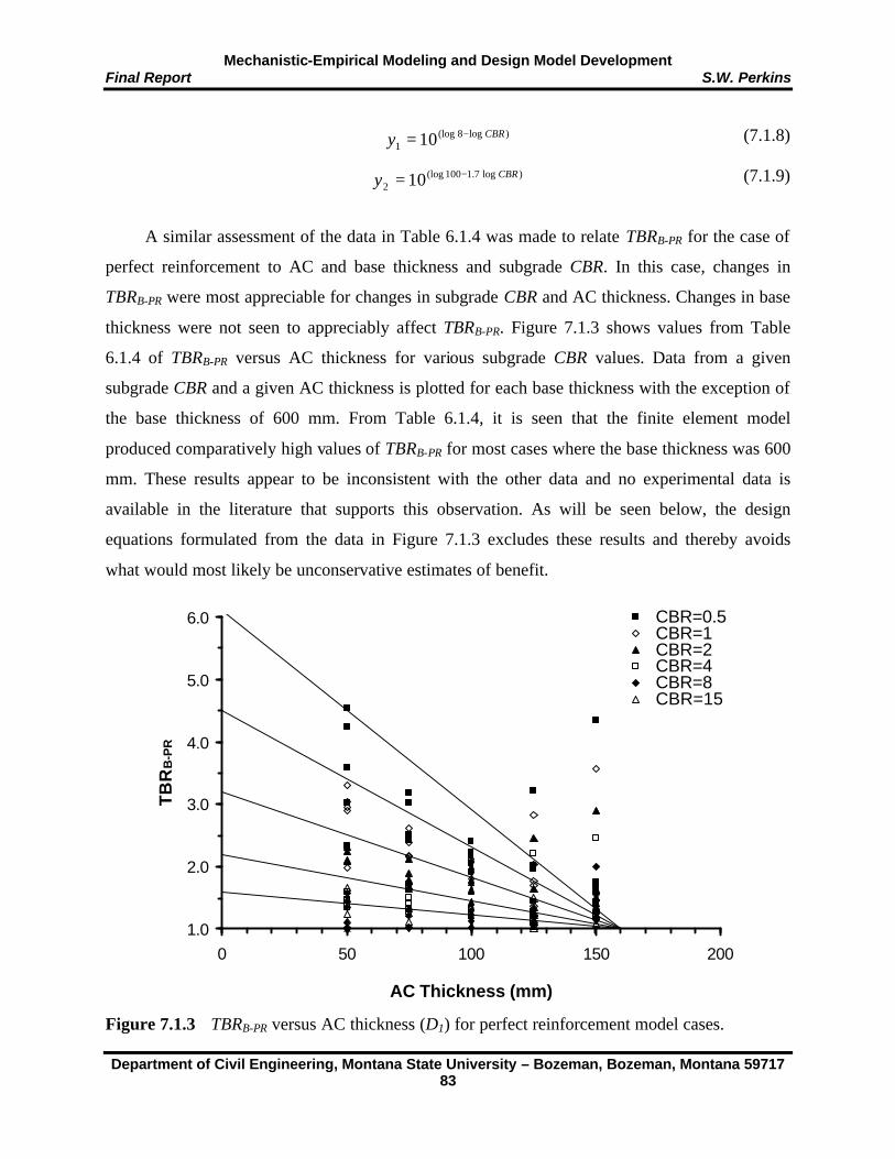
Mechanistic-Empirical Modeling and Design Model Development Final Report S.W. Perkins
Department of Civil Engineering, Montana State University – Bozeman, Bozeman, Montana 59717 83
)log8(log1 10 CBRy −=
)log7.1100(log2 10 CBRy −=
(7.1.8)
(7.1.9)
A similar assessment of the data in Table 6.1.4 was made to relate TBRB-PR for the case of
perfect reinforcement to AC and base thickness and subgrade CBR. In this case, changes in
TBRB-PR were most appreciable for changes in subgrade CBR and AC thickness. Changes in base
thickness were not seen to appreciably affect TBRB-PR. Figure 7.1.3 shows values from Table
6.1.4 of TBRB-PR versus AC thickness for various subgrade CBR values. Data from a given
subgrade CBR and a given AC thickness is plotted for each base thickness with the exception of
the base thickness of 600 mm. From Table 6.1.4, it is seen that the finite element model
produced comparatively high values of TBRB-PR for most cases where the base thickness was 600
mm. These results appear to be inconsistent with the other data and no experimental data is
available in the literature that supports this observation. As will be seen below, the design
equations formulated from the data in Figure 7.1.3 excludes these results and thereby avoids
what would most likely be unconservative estimates of benefit.
Figure 7.1.3 TBRB-PR versus AC thickness (D1) for perfect reinforcement model cases.
1.0
2.0
3.0
4.0
5.0
6.0
0 50 100 150 200
AC Thickness (mm)
TB
RB
-PR
CBR=0.5CBR=1CBR=2CBR=4CBR=8CBR=15Series7Series8
Mechanistic-Empirical Modeling and Design Model Development Final Report S.W. Perkins
Department of Civil Engineering, Montana State University – Bozeman, Bozeman, Montana 59717 84
bD
bTBR PRB +−=− 160)1( 1
522.045.4 −= CBRb
From Figure 7.1.3 it is seen that more scatter is observed for results of TBRB-PR as
compared to those observed in Figure 7.1.1 for TBRS-PR. The values of TBRB-PR are, however,
relatively modest in comparison to TBRS-PR. Due to this scatter, relatively simple and
conservative estimates of the data were developed by straight-lines in an arithmetic plot of TBRB-
PR versus AC thickness for various subgrade CBR’s. The equation of these lines is given by:
(7.1.10)
where D1 is the AC thickness in units of mm and b is the y-intercept of the lines. Values of b
were related to subgrade CBR through Equation 7.1.11. The lines shown in Figure 7.1.3 result
from the use of Equations 7.1.10 and 7.1.11.
(7.1.11)
7.1.2 Equations for BCR and TBR/BCR Combinations for Perfect Reinforcement
In Section 6.1, 450 comparisons between unreinforced and perfect reinforced models with a
reduced base course thickness were available. For each comparison run, a combination of BCR
and TBR was available, where TBR was broken into components of TBRB and TBRS for each
case. The introduction of a new input variable (base course thickness reduction) made it difficult
to develop regression equations that reasonably described the results obtained. A simple method
was therefore sought for relating combinations of BCR and TBR to pavement design parameters.
The method chosen is described below and is based on existing pavement design principles and
methodologies. The method has not been validated against results from test sections, but is
compared to results obtained from the finite element model cases described in Section 6.1 in
order to assess its reasonableness and degree of safety.
The method relies upon the use of design equations contained in the AASHTO ’93
pavement design guide (AASHTO, 1993). The approach was outlined in Berg et al. (2000) and
is developed in greater detail below. The method relies upon the knowledge of a TBR for
equivalent unreinforced and reinforced sections (i.e. TBR for BCR = 0). The AASHTO ’93
pavement design equation is then used to calculate an increased structural layer coefficient for
the base course aggregate for the reinforced section that gives the increased number of ESAL’s

Mechanistic-Empirical Modeling and Design Model Development Final Report S.W. Perkins
Department of Civil Engineering, Montana State University – Bozeman, Bozeman, Montana 59717 85
22211 mDaDaSN +=
CBRM S 1500=
that this section can carry for the case where no base course thickness reduction is used. The new
base layer coefficient is then used to determine the base course thickness reduction such that
equal life or ESAL’s is predicted for the reinforced and unreinforced pavement (i.e. BCR when
TBR = 1). The method can also be used to calculate the remaining BCR for an assumed TBR or to
calculate the remaining TBR for an assumed BCR.
An unreinforced pavement design cross section is first presumed to be known. The AC and
base thickness and layer coefficients, and the subgrade CBR or resilient modulus is required.
With these parameters, the 1993 AASHTO pavement design equation is used to calculate the
number of ESAL’s for the unreinforced pavement (W18-U) from Equations 7.1.12 and 7.1.13.
(7.1.12)
(7.1.13)
In Equations 7.1.12 and 7.1.13, ZR is the standard normal deviate, So is the combined standard
error, ∆PSI is the loss of design serviceability, MS is the effective roadbed (subgrade) resilient
modulus in units of psi, a1 and a2 are the layer coefficients of the asphalt concrete and base
aggregate layers, respectively, D1 and D2 are the thicknesses of the AC and base layers,
respectively, and m2 is the drainage coefficient of the base layer. Values of ZR, So, ∆PSI, a1, a2
and m2 have been taken as constants for the development of this method and have been given
values of –1.645, 0.35 and 1.9, 0.4, 0.14 and 1.0, respectively, where the value of ZR corresponds
to a reliability of 95 %. Values of MS in units of psi are related to subgrade CBR through
Equation 7.1.14.
(7.1.14)
A known value of TBR when BCR = 0 then allows W18 to be calculated from Equation 7.1.15 for
a reinforced pavement having identical pavement layer thicknesses and properties. In Equation
7.1.15, the TBR used may correspond to TBRB, TBRS or TBRT.
( )
( )
−+
++
−∆
+−++=− 07.8)log(32.2
11094
4.0
5.12.4log
2.01log36.9^10
19.5
18 SoRU M
SN
PSI
SNSZW
Mechanistic-Empirical Modeling and Design Model Development Final Report S.W. Perkins
Department of Civil Engineering, Montana State University – Bozeman, Bozeman, Montana 59717 86
TBRWW UR −− = 1818
22
112 ma
DaSND
R
UR
−−
−=
U
RU
DDD
BCR−
−− −=
2
22100
UR DBCR
D −−
−= 22 1001
(7.1.15)
The value of W18-R from Equation 7.1.15 is then used in Equation 7.1.12 to calculate a value of
SN for the reinforced pavement, with this value used in Equation 7.1.13 to determine a new value
of a2 for the reinforced pavement, with all other parameters in Equations 7.1.12 and 7.1.13 being
equal to those used for the unreinforced pavement. This approach assumes that the TBR seen for
the comparative reinforced and unreinforced pavments can be accounted for by an increased
structural base layer coefficient. This calculation requires an iterative solution for SN in Equation
7.1.12. Once a value of a2 for the reinforced pavement is obtained (a2-R), this value is used in
Equation 7.1.13 along with a reduced base thickness for the reinforced pavement (D2-R) such that
a SN identical to the unreinforced pavement is obtained. The reduced base thickness is calculated
from
(7.1.16)
This allows for the determination of a value of BCR when TBR = 1 from Equation 7.1.17.
Depending on the value of TBR used in Equation 7.1.15 (TBRB, TBRS or TBRT), the computed
BCR then pertains to reinforcement effects on the base, subgrade or total system.
(7.1.17)
With this approach, values of TBR when BCR=0 and BCR when TBR=1 are known. If a
value of TBR less than TBRBCR=0 is used, it should be expected that the remaining benefit can be
expressed in terms of a BCR. Conversely, if a value of BCR less than BCRTBR=1 is used,
remaining benefit can be expressed in terms of a TBR. The same general approach described
above is used to determine combinations of BCR and TBR. Each approach uses the
predetermined value of TBRBCR=0 to determine the increased structural base layer coefficient of
the reinforced pavement. For the case where a desired BCR is specified, the reinforced base layer
thickness is determined from Equation 7.1.18.
(7.1.18)

Mechanistic-Empirical Modeling and Design Model Development Final Report S.W. Perkins
Department of Civil Engineering, Montana State University – Bozeman, Bozeman, Montana 59717 87
22211 mDaDaSN RRR −−+=
U
R
WW
TBR−
−=18
18
22
112 ma
DaSND
R
RR
−−
−=
Structural number of the reinforced pavement is then determined from Equation 7.1.19.
(7.1.19)
where a2-R is determined from the method described above and by knowing the value of
TBRBCR=0. A value of W18-R is then determined using Equation 7.1.12 using the value of SN from
Equation 7.1.19. A value of remaining TBR is then computed by Equation 7.1.20, where this
value should lie between 1 and TBRBCR=0, provided the desired value of BCR used was less than
or equal to BCRTBR=1.
(7.1.20)
For the case where a desired TBR is specified, Equation 7.1.15 is used to calculate the
number of ESAL’s required of the reinforced section. Equation 7.1.12 is then solved iteratively
to give the required SN for the reinforced section (SNR). Equation 7.1.21 is then used to
determine the base layer thickness necessary to produce this SN, where the reinforced structural
base layer coefficient is used in this equation.
(7.1.21)
The remaining BCR is then determined from Equation 7.1.17, where the value obtained should
lie between 0 and BCRTBR=1, provided the desired value of TBR was less than TBRBCR=0.
The above approach has not been validated previously by either test section results or
comparisons to numerical models. To evaluate the reasonableness of this approach, the above
method was compared to results from the parametric study for the case of perfect reinforcement.
As described in Section 6.1, 450 comparisons of finite element cases were made to assess
combinations of TBR and BCR from the response measures derived from the models. For these
comparisons, an assumed or desired value of BCR was used to create the models. The response
measures were then used to define the remaining TBR. As described previously, the response
measures were used to define partial TBR’s for the subgrade (TBRS) and base (TBRB) with the
product of the two defining the total TBR (TBRT). Combinations of BCR and TBR for each of the
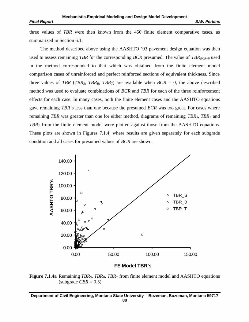
Mechanistic-Empirical Modeling and Design Model Development Final Report S.W. Perkins
Department of Civil Engineering, Montana State University – Bozeman, Bozeman, Montana 59717 88
three values of TBR were then known from the 450 finite element comparative cases, as
summarized in Section 6.1.
The method described above using the AASHTO ’93 pavement design equation was then
used to assess remaining TBR for the corresponding BCR presumed. The value of TBRBCR=0 used
in the method corresponded to that which was obtained from the finite element model
comparison cases of unreinforced and perfect reinforced sections of equivalent thickness. Since
three values of TBR (TBRS, TBRB, TBRT) are available when BCR = 0, the above described
method was used to evaluate combinations of BCR and TBR for each of the three reinforcement
effects for each case. In many cases, both the finite element cases and the AASHTO equations
gave remaining TBR’s less than one because the presumed BCR was too great. For cases where
remaining TBR was greater than one for either method, diagrams of remaining TBRS, TBRB and
TBRT from the finite element model were plotted against those from the AASHTO equations.
These plots are shown in Figures 7.1.4, where results are given separately for each subgrade
condition and all cases for presumed values of BCR are shown.
Figure 7.1.4a Remaining TBRS, TBRB, TBRT from finite element model and AASHTO equations (subgrade CBR = 0.5).
0.00
20.00
40.00
60.00
80.00
100.00
120.00
140.00
0.00 50.00 100.00 150.00
FE Model TBR's
AA
SH
TO
TB
R's
TBR_S
TBR_B
TBR_T
Series4

Mechanistic-Empirical Modeling and Design Model Development Final Report S.W. Perkins
Department of Civil Engineering, Montana State University – Bozeman, Bozeman, Montana 59717 89
Figure 7.1.4b Remaining TBRS, TBRB, TBRT from finite element model and AASHTO equations (subgrade CBR = 1).
Figure 7.1.4c Remaining TBRS, TBRB, TBRT from finite element model and AASHTO equations
(subgrade CBR = 2).
1.00
3.00
5.00
7.00
9.00
11.00
13.00
15.00
1.00 3.00 5.00 7.00 9.00 11.00 13.00 15.00
FE Model TBR's
AA
SH
TO
TB
R's TBR_S
TBR_B
TBR_T
Series4
1.00
3.00
5.00
7.00
9.00
11.00
13.00
15.00
1.00 3.00 5.00 7.00 9.00 11.00 13.00 15.00
FE Model TBR's
AA
SH
TO
TB
R's TBR_S
TBR_B
TBR_T
Series4

Mechanistic-Empirical Modeling and Design Model Development Final Report S.W. Perkins
Department of Civil Engineering, Montana State University – Bozeman, Bozeman, Montana 59717 90
Figure 7.1.4d Remaining TBRS, TBRB, TBRT from finite element model and AASHTO equations (subgrade CBR = 4).
Figure 7.1.4e Remaining TBRS, TBRB, TBRT from finite element model and AASHTO equations (subgrade CBR = 8).
1.00
2.00
3.00
4.00
5.00
1.00 2.00 3.00 4.00 5.00
FE Model TBR's
AA
SH
TO
TB
R's
TBR_S
TBR_B
TBR_T
Series4
1.00
2.00
3.00
4.00
5.00
1.00 2.00 3.00 4.00 5.00
FE Model TBR's
AA
SH
TO
TB
R's
TBR_S
TBR_B
TBR_T
Series4
Mechanistic-Empirical Modeling and Design Model Development Final Report S.W. Perkins
Department of Civil Engineering, Montana State University – Bozeman, Bozeman, Montana 59717 91
The results seen in Figure 7.1.4 indicate that the use of the AASHTO equations is
conservative with respect to that obtained from the finite element model for all TBR measures
and for all subgrade cases except for the CBR = 0.5 case. Due to the apparent unconservative
nature of this method for CBR = 0.5 and the decreased margin of safety when designing for a
BCR at low values of subgrade CBR, it is recommended that this method described above for
calculating BCR or TBR/BCR combinations be used only for designs with a subgrade CBR $ 1.
7.2 Influence of Geosynthetic Isotropic Elastic Modulus on TBR
Section 7.1 presented equations for determination of partial and total values of TBR (TBRS,
TBRB, TBRT) when BCR = 0 and a method for calculating either BCRTBR=0 or combinations of
BCR and TBR for the condition of perfect reinforcement. The addition of a new variable, namely
geosynthetic isotropic modulus, precluded evaluating all 180 cases previously examined for the
case of perfect reinforcement for each of the five values of reinforcement elastic modulus given
in Section 6.2.1. Particular model cases were chosen for evaluation of each of the five
reinforcement elastic modulus values. Section 6.2.1 described 250 additional finite element
model cases created to examine the effect of the elastic modulus of the reinforcement on TBR.
These cases were chosen to provide information on how values of geosynthetic isotropic elastic
modulus reduced the TBR seen for the case of perfect reinforcement for critical cases.
The equations developed in Section 7.1 for the determination of TBRS-PR, and as shown in
Figure 7.1.1, showed that two straight lines in a semi-log plot of TBRS-PR versus section SN could
approximate values of TBRS-PR for perfect reinforcement, where the equations for these lines was
a function of the subgrade CBR. Key points along these curves correspond to values of SN of 1.6,
3.3 and for larger values of SN where TBRS-PR is seen to return to a value of 1. The three sets of
model cases shown in Table 6.2.2 were chosen to provide results for sections with values of SN
close to each of these three values. Three sections within each set were chosen to provide
redundancy.
The effect of geosynthetic isotropic elastic modulus was expressed in terms of a reduction
factor applied to the value of TBRS-PR obtained for the corresponding case of perfect
reinforcement, where this reduction factor for geosynthetic isotropic modulus (RFGM) is given by
Equation 7.2.1. The reduction factor is expressed as a percentage and is relative to a TBR
baseline value of 1.
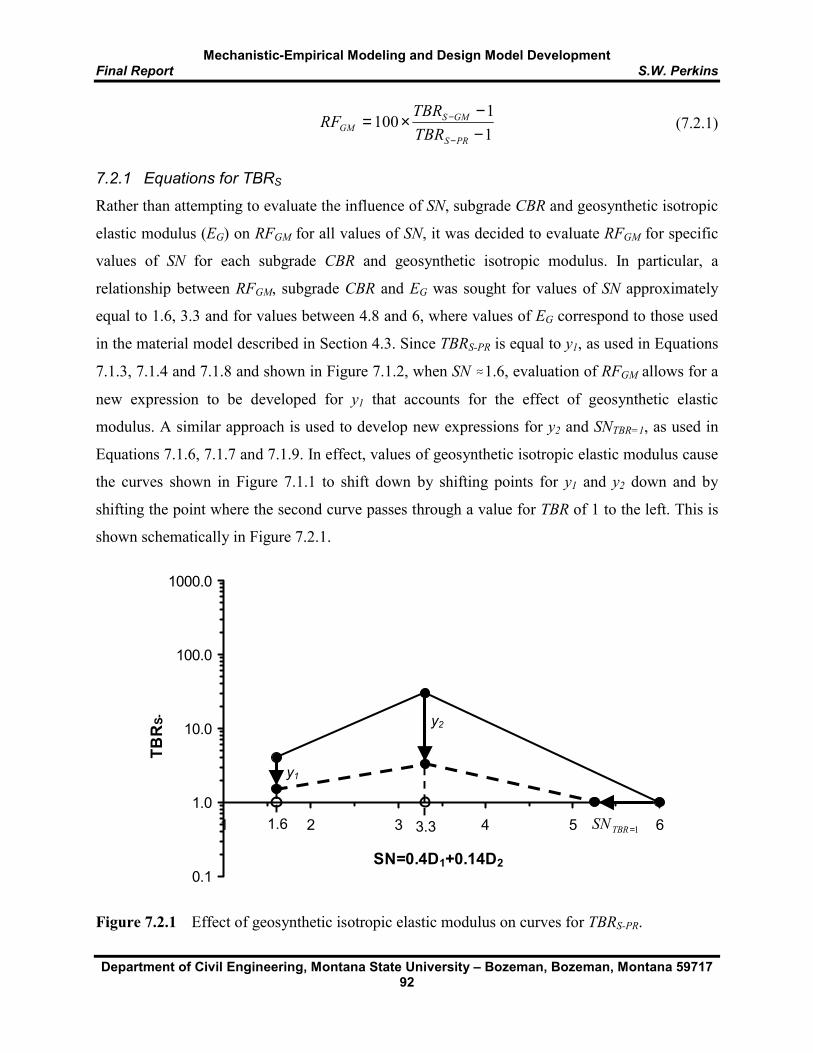
Mechanistic-Empirical Modeling and Design Model Development Final Report S.W. Perkins
Department of Civil Engineering, Montana State University – Bozeman, Bozeman, Montana 59717 92
11
100−−
×=−
−
PRS
GMSGM TBR
TBRRF
(7.2.1)
7.2.1 Equations for TBRS
Rather than attempting to evaluate the influence of SN, subgrade CBR and geosynthetic isotropic
elastic modulus (EG) on RFGM for all values of SN, it was decided to evaluate RFGM for specific
values of SN for each subgrade CBR and geosynthetic isotropic modulus. In particular, a
relationship between RFGM, subgrade CBR and EG was sought for values of SN approximately
equal to 1.6, 3.3 and for values between 4.8 and 6, where values of EG correspond to those used
in the material model described in Section 4.3. Since TBRS-PR is equal to y1, as used in Equations
7.1.3, 7.1.4 and 7.1.8 and shown in Figure 7.1.2, when SN .1.6, evaluation of RFGM allows for a
new expression to be developed for y1 that accounts for the effect of geosynthetic elastic
modulus. A similar approach is used to develop new expressions for y2 and SNTBR=1, as used in
Equations 7.1.6, 7.1.7 and 7.1.9. In effect, values of geosynthetic isotropic elastic modulus cause
the curves shown in Figure 7.1.1 to shift down by shifting points for y1 and y2 down and by
shifting the point where the second curve passes through a value for TBR of 1 to the left. This is
shown schematically in Figure 7.2.1.
Figure 7.2.1 Effect of geosynthetic isotropic elastic modulus on curves for TBRS-PR.
0.1
1.0
10.0
100.0
1000.0
1 2 3 4 5 6
SN=0.4D1+0.14D2
TBR
S-PR
1.6 3.3 1=TBRSN
y2
y1
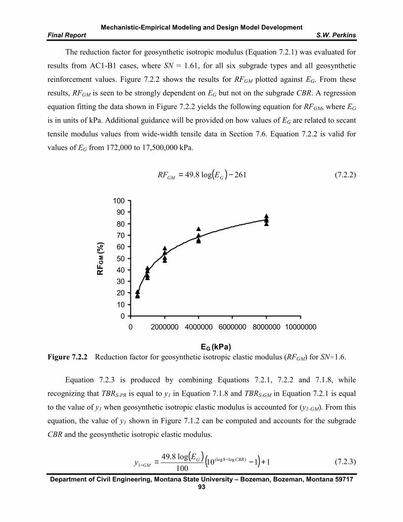
Mechanistic-Empirical Modeling and Design Model Development Final Report S.W. Perkins
Department of Civil Engineering, Montana State University – Bozeman, Bozeman, Montana 59717 93
( ) 261log8.49 −= GGM ERF
( ) ( ) 1110100log8.49 )log8(log
1 +−= −−
CBRGGM
Ey
The reduction factor for geosynthetic isotropic modulus (Equation 7.2.1) was evaluated for
results from AC1-B1 cases, where SN = 1.61, for all six subgrade types and all geosynthetic
reinforcement values. Figure 7.2.2 shows the results for RFGM plotted against EG. From these
results, RFGM is seen to be strongly dependent on EG but not on the subgrade CBR. A regression
equation fitting the data shown in Figure 7.2.2 yields the following equation for RFGM, where EG
is in units of kPa. Additional guidance will be provided on how values of EG are related to secant
tensile modulus values from wide-width tensile data in Section 7.6. Equation 7.2.2 is valid for
values of EG from 172,000 to 17,500,000 kPa.
(7.2.2)
Figure 7.2.2 Reduction factor for geosynthetic isotropic elastic modulus (RFGM) for SN.1.6.
Equation 7.2.3 is produced by combining Equations 7.2.1, 7.2.2 and 7.1.8, while
recognizing that TBRS-PR is equal to y1 in Equation 7.1.8 and TBRS-GM in Equation 7.2.1 is equal
to the value of y1 when geosynthetic isotropic elastic modulus is accounted for (y1-GM). From this
equation, the value of y1 shown in Figure 7.1.2 can be computed and accounts for the subgrade
CBR and the geosynthetic isotropic elastic modulus.
(7.2.3)
0102030405060708090
100
0 2000000 4000000 6000000 8000000 10000000
EG (kPa)
RF G
M (%
)

Mechanistic-Empirical Modeling and Design Model Development Final Report S.W. Perkins
Department of Civil Engineering, Montana State University – Bozeman, Bozeman, Montana 59717 94
GGM EmRF =
66 1057.1)log(108.1 −− ×+×= CBRm
( ) ( ) 1110100
1057.1log108.1 )log7.1100(log66
2 +−×+×= −−−
−CBR
GGM ECBRy
0504.0028.01 )28.0(54.2 GTBR ECBRSN
GMS−==−
Finite element models corresponding to the second set listed in Table 6.2.2, where values
of SN ranged between 2.99 and 3.62, were used to evaluate the influence of reinforcement
isotropic elastic modulus on values of y2. A reduction factor for isotropic elastic modulus was
defined for these results according to Equation 7.2.1, where for these cases it is recognized that
TBRS-PR is equal to y2 in Equation 7.1.9 and TBRS-GM is equal to the value of y2 when
geosynthetic isotropic modulus is accounted for (y2-GM). Figure 7.2.3 shows RFGM plotted against
EG. For these results, it is seen that RFGM is influenced by both reinforcement isotropic elastic
modulus and subgrade CBR. Reduction factors become more significant as reinforcement
modulus decreases and as subgrade CBR decreases. Straight lines were used to approximate the
trends seen in the data, as shown in Figure 7.2.3, where each line extends through the origin and
is given by Equation 7.2.4. The slope of the lines, m, was plotted against the subgrade CBR, as
shown in Figure 7.2.4, with Equation 7.2.5 providing the best fit curve shown. Combination of
Equations 7.2.4, 7.2.5, 7.2.2 and 7.1.9 yields a new equation for y2 that accounts for
reinforcement isotropic elastic modulus and subgrade CBR, where EG is in units of kPa.
(7.2.4)
(7.2.5)
(7.2.6)
The effect of reinforcement isotropic elastic modulus on values of SNTBR=1 were
evaluated by first using Equation 7.2.6 to calculate the value of y2-GM for each value of isotropic
elastic modulus and subgrade CBR given in Table 6.2.2. Each value of y2-GM corresponds to
TBRS-GM for a SN=3.3. For the corresponding finite element cases for AC5-B5 where SN=4.57, a
value of TBRS-GM is known. Based on these two points, a straight line in a semi-log plot of TBRS-
GM versus SN is used to estimate a value for SN when TBRS-GM = 1. Regression equations between
these values and EG and subgrade CBR were then developed, with Equation 7.2.7 being the
result.
(7.2.7)
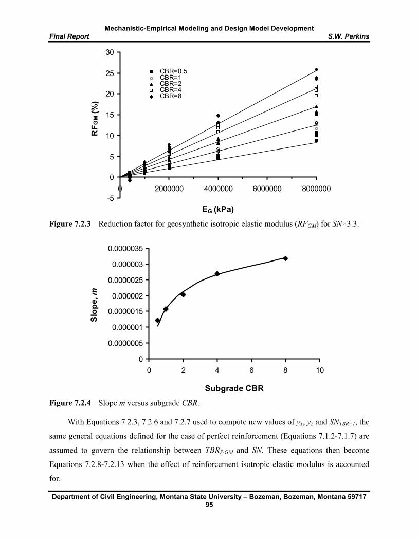
Mechanistic-Empirical Modeling and Design Model Development Final Report S.W. Perkins
Department of Civil Engineering, Montana State University – Bozeman, Bozeman, Montana 59717 95
Figure 7.2.3 Reduction factor for geosynthetic isotropic elastic modulus (RFGM) for SN.3.3. Figure 7.2.4 Slope m versus subgrade CBR. With Equations 7.2.3, 7.2.6 and 7.2.7 used to compute new values of y1, y2 and SNTBR=1, the
same general equations defined for the case of perfect reinforcement (Equations 7.1.2-7.1.7) are
assumed to govern the relationship between TBRS-GM and SN. These equations then become
Equations 7.2.8-7.2.13 when the effect of reinforcement isotropic elastic modulus is accounted
for.
-5
0
5
10
15
20
25
30
0 2000000 4000000 6000000 8000000
EG (kPa)
RF G
M (%
)
CBR=0.5CBR=1CBR=2CBR=4CBR=8Series6Series7
0
0.0000005
0.000001
0.0000015
0.000002
0.0000025
0.000003
0.0000035
0 2 4 6 8 10
Subgrade CBR
Slop
e, m
Mechanistic-Empirical Modeling and Design Model Development Final Report S.W. Perkins
Department of Civil Engineering, Montana State University – Bozeman, Bozeman, Montana 59717 96
)log( 11103.36.1 oySNmGMSTBRSN +
− =≤≤
7.1
log1
2
1GM
GM
yy
m −
−
=
)6.1(1
1 110 mGM
oy
y −=
)log( 22100.63.3 oySNmGMSTBRSN +
− =≤≤
3.3log
)1(
22 −
−=
=
−
−GMSTBR
GM
SNy
m
)3.3(2
2 210 mGM
oy
y −=
288)log(8.55 −= GGM ERF
(7.2.8)
(7.2.9)
(7.2.10)
(7.2.11)
(7.2.12)
(7.2.13)
7.2.2 Equations for TBRB
Reduction factors were also developed to modify values of TBRB-PR for the case of perfect
reinforcement to account for values of geosynthetic isotropic elastic modulus. Evaluation of all
cases contained in Table 6.2.2 indicated that the reduction factor for modulus was dependent
most strongly on only the reinforcement modulus. The reduction factor developed, having the
same general definition as that given in Equation 7.2.1, is given by Equation 7.2.14, where this
equation is valid for values of EG between 143,000 and 8,835,000 kPa.
(7.2.14)
Combination of Equations 7.2.14, 7.2.1, 7.1.10 and 7.1.11 yields Equation 7.2.15 for
determination of TBRB-GM accounting for the influences of subgrade CBR, AC thickness and
reinforcement isotropic modulus. The use of Equation 7.2.15 for the conditions present in the
finite element cases given in Table 6.2.2 is compared in Figure 7.2.5 to the values of TBRB
computed directly from the finite element results. From this figure it is seen that the combination
of the equation used for the TBRB-PR (Equations 7.1.10 and 7.1.11) and the equation used for the
reduction factor (Equation 7.2.14) results in conservative estimates of TBRB when compared to

Mechanistic-Empirical Modeling and Design Model Development Final Report S.W. Perkins
Department of Civil Engineering, Montana State University – Bozeman, Bozeman, Montana 59717 97
( ) 1145.4160
45.41100
288)log(8.55 522.01522.0 +
−+−
−= −−
− CBRD
CBRE
TBR GGMB
GM
GMRGMR TBR
TBRRF =
results obtained directly from the finite element model and is also seen to eliminate some of the
high values predicted for certain sections with a large base thickness.
(7.2.15)
Figure 7.2.5 TBRB comparison from FE model and Equation 7.2.15.
7.3 Influence of Geosynthetic Modulus Anisotropy on TBR
Effects of anisotropy of the elastic modulus of the geosynthetic between the machine and cross-
machine directions were evaluated by comparison of values of TBR obtained from the model
cases listed in Table 6.2.4 to corresponding cases with isotropic modulus values. Design
equations for TBRS-GM and TBRB-GM were developed in Section 7.2 and were given by Equations
7.2.8-7.2.13 and 7.2.15, respectively. A reduction factor for geosynthetic modulus ratio was
defined according to Equation 7.3.1 and evaluated for the finite element model cases listed in
Table 6.2.4. Reduction factors were evaluated for corresponding TBR values for subgrade and
base reinforcement effects.
(7.3.1)
1
10
1 10
TBRB from FE Cases
TB
RB fr
om D
esig
n E
quat
ion
7.2.
15
Mechanistic-Empirical Modeling and Design Model Development Final Report S.W. Perkins
Department of Civil Engineering, Montana State University – Bozeman, Bozeman, Montana 59717 98
mGmRF MRGMR −+= 1
)log(62.0 GMSTBRm −=
max
min
−
−=G
GMR E
EG
[ ])log(62.01)log(62.0 GMSMRGMSGMSGMRS TBRGTBRTBRTBR −−−− −+=
( )8.02.0 += −− MRGMBGMRB GTBRTBR
For values of TBRS, values of RFGMR were found to be approximated by straight line
relationships given by Equation 7.3.2, where m is the slope of the lines and was seen to be a
function of TBRS-GM, as given by Equation 7.3.3 and GMR is the ratio of moduli and is given by
Equation 7.3.4.
(7.3.2)
(7.3.3)
(7.3.4)
Combination of Equations 7.3.1, 7.3.2 and 7.3.3 yields Equation 7.3.5.
(7.3.5)
A similar analysis for values of TBRB showed that the reduction factor was dependent
primarily on GMR, which allowed Equation 7.3.6 to be developed.
(7.3.6)
Evaluation of TBRS-GM and TBRB-GM from Equations 7.2.8-7.2.13 and 7.2.15, respectively, for
the case of isotropic geosynthetic modulus values allows these values to be reduced by the use of
Equations 7.3.5 and 7.3.6 when GMR from Equation 7.3.4 is evaluated.
7.4 Influence of Geosynthetic Poisson’s Ratio and Shear Modulus on TBR
The finite element model cases presented in Tables 6.2.5 and 6.2.6 were used to examine the
effect of reducing Poisson’s ratio and shear modulus to zero from the values used for the case of
isotropic material properties. A reduction factor was computed for the effect of reducing each
variable according to Equations 7.4.1 and 7.4.2, where TBRν and TBRG were values of TBR
obtained directly from the cases examined where either ν or G was reduced to zero and TBRGM

Mechanistic-Empirical Modeling and Design Model Development Final Report S.W. Perkins
Department of Civil Engineering, Montana State University – Bozeman, Bozeman, Montana 59717 99
GMG TBR
TBRRF ν
ν =
GM
GGG TBR
TBRRF =
GM
GGG TBR
TBRRF ν
ν =
was the TBR for the corresponding model case where isotropic elastic values were used for the
geosynthetic material. A reduction factor was also computed for the combined effect of reducing
both ν and G according to Equation 7.4.3. Geosynthetic property cases from Table 6.2.5 of
GνG3 and GνG4 were used to evaluate RFGν. Cases GνG5 and GνG6 were used to evaluate
RFGG. Cases GνG7 and GνG8 were used to evaluate RFGνG. Reduction factors for both values of
TBRS and TBRB were evaluated.
(7.4.1)
(7.4.2)
(7.4.3)
Table 7.4.1 summarizes average values of reduction factors obtained for each
reinforcement effect (i.e. base and subgrade). From these results, it appears that the combined
effect of reducing both Poisson’s ratio and shear modulus to zero corresponds to the product of
the two reduction factors for each individual effect. Based on these results, reduction factors can
be used either individually or in series and applied to TBRS-GM and TBRB-GM for reduction of
these TBR’s according to Equations 7.4.1-7.4.3.
Table 7.4.1 Reduction factors for reinforcement Poisson’s ratio and shear modulus. RFGν RFGG RFGνG TBRS 0.83 0.92 0.75 TBRB 0.96 0.99 0.95
7.5 Influence of Interface Properties on TBR
Specific finite element model cases were not created to examine the effect of varying
geosynthetic-base aggregate interface properties for the reasons described in Section 4.3, where
it was argued that the influence of interface shear properties should be accounted for by
comparison of predictions from the design model to test section results. The computation of TBR
accounting for all the effects described above implicitly assumes optimal interface properties. A
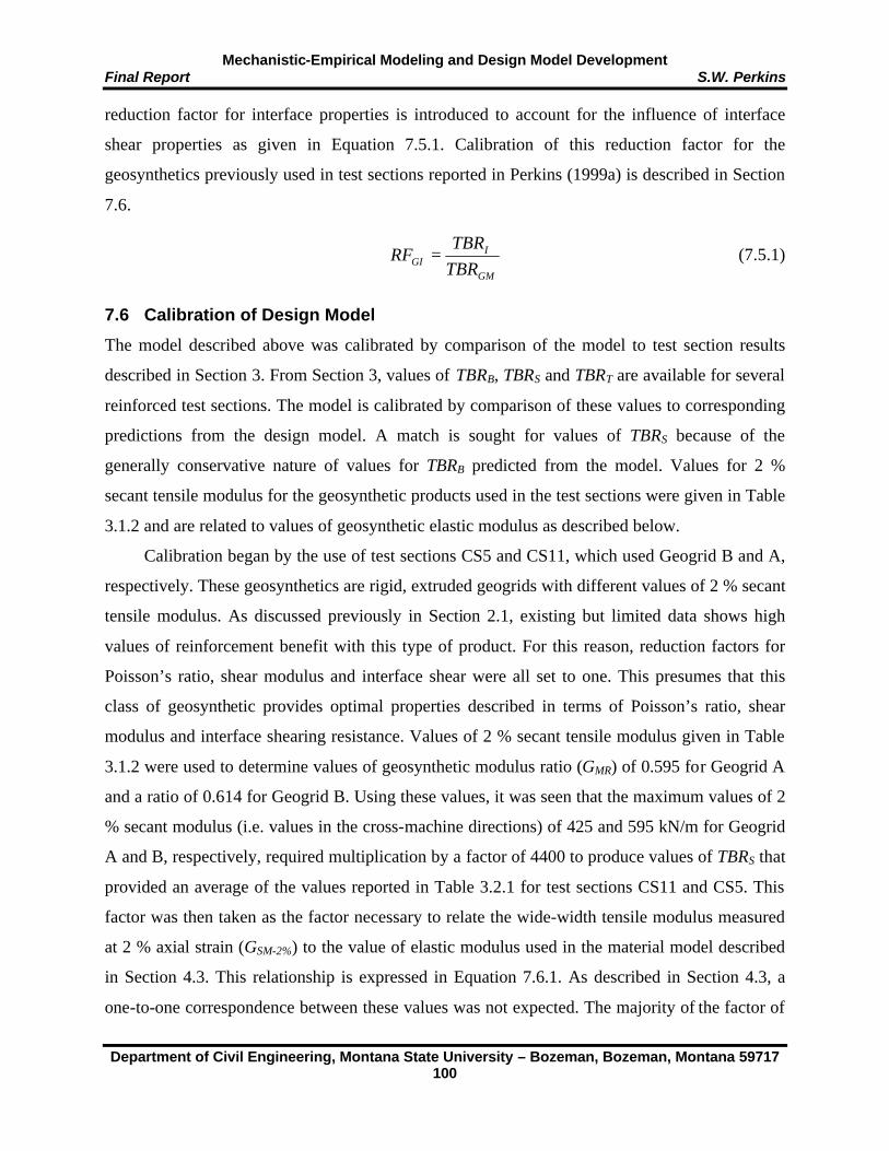
Mechanistic-Empirical Modeling and Design Model Development Final Report S.W. Perkins
Department of Civil Engineering, Montana State University – Bozeman, Bozeman, Montana 59717 100
GM
IGI TBR
TBRRF =
reduction factor for interface properties is introduced to account for the influence of interface
shear properties as given in Equation 7.5.1. Calibration of this reduction factor for the
geosynthetics previously used in test sections reported in Perkins (1999a) is described in Section
7.6.
(7.5.1)
7.6 Calibration of Design Model
The model described above was calibrated by comparison of the model to test section results
described in Section 3. From Section 3, values of TBRB, TBRS and TBRT are available for several
reinforced test sections. The model is calibrated by comparison of these values to corresponding
predictions from the design model. A match is sought for values of TBRS because of the
generally conservative nature of values for TBRB predicted from the model. Values for 2 %
secant tensile modulus for the geosynthetic products used in the test sections were given in Table
3.1.2 and are related to values of geosynthetic elastic modulus as described below.
Calibration began by the use of test sections CS5 and CS11, which used Geogrid B and A,
respectively. These geosynthetics are rigid, extruded geogrids with different values of 2 % secant
tensile modulus. As discussed previously in Section 2.1, existing but limited data shows high
values of reinforcement benefit with this type of product. For this reason, reduction factors for
Poisson’s ratio, shear modulus and interface shear were all set to one. This presumes that this
class of geosynthetic provides optimal properties described in terms of Poisson’s ratio, shear
modulus and interface shearing resistance. Values of 2 % secant tensile modulus given in Table
3.1.2 were used to determine values of geosynthetic modulus ratio (GMR) of 0.595 for Geogrid A
and a ratio of 0.614 for Geogrid B. Using these values, it was seen that the maximum values of 2
% secant modulus (i.e. values in the cross-machine directions) of 425 and 595 kN/m for Geogrid
A and B, respectively, required multiplication by a factor of 4400 to produce values of TBRS that
provided an average of the values reported in Table 3.2.1 for test sections CS11 and CS5. This
factor was then taken as the factor necessary to relate the wide-width tensile modulus measured
at 2 % axial strain (GSM-2%) to the value of elastic modulus used in the material model described
in Section 4.3. This relationship is expressed in Equation 7.6.1. As described in Section 4.3, a
one-to-one correspondence between these values was not expected. The majority of the factor of
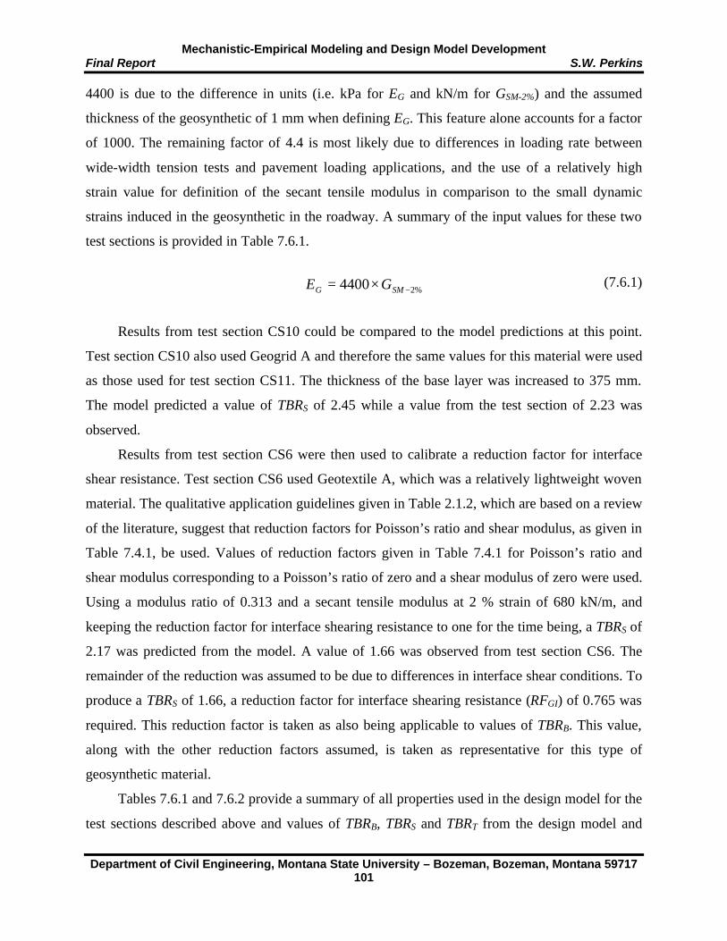
Mechanistic-Empirical Modeling and Design Model Development Final Report S.W. Perkins
Department of Civil Engineering, Montana State University – Bozeman, Bozeman, Montana 59717 101
%24400 −×= SMG GE
4400 is due to the difference in units (i.e. kPa for EG and kN/m for GSM-2%) and the assumed
thickness of the geosynthetic of 1 mm when defining EG. This feature alone accounts for a factor
of 1000. The remaining factor of 4.4 is most likely due to differences in loading rate between
wide-width tension tests and pavement loading applications, and the use of a relatively high
strain value for definition of the secant tensile modulus in comparison to the small dynamic
strains induced in the geosynthetic in the roadway. A summary of the input values for these two
test sections is provided in Table 7.6.1.
(7.6.1)
Results from test section CS10 could be compared to the model predictions at this point.
Test section CS10 also used Geogrid A and therefore the same values for this material were used
as those used for test section CS11. The thickness of the base layer was increased to 375 mm.
The model predicted a value of TBRS of 2.45 while a value from the test section of 2.23 was
observed.
Results from test section CS6 were then used to calibrate a reduction factor for interface
shear resistance. Test section CS6 used Geotextile A, which was a relatively lightweight woven
material. The qualitative application guidelines given in Table 2.1.2, which are based on a review
of the literature, suggest that reduction factors for Poisson’s ratio and shear modulus, as given in
Table 7.4.1, be used. Values of reduction factors given in Table 7.4.1 for Poisson’s ratio and
shear modulus corresponding to a Poisson’s ratio of zero and a shear modulus of zero were used.
Using a modulus ratio of 0.313 and a secant tensile modulus at 2 % strain of 680 kN/m, and
keeping the reduction factor for interface shearing resistance to one for the time being, a TBRS of
2.17 was predicted from the model. A value of 1.66 was observed from test section CS6. The
remainder of the reduction was assumed to be due to differences in interface shear conditions. To
produce a TBRS of 1.66, a reduction factor for interface shearing resistance (RFGI) of 0.765 was
required. This reduction factor is taken as also being applicable to values of TBRB. This value,
along with the other reduction factors assumed, is taken as representative for this type of
geosynthetic material.
Tables 7.6.1 and 7.6.2 provide a summary of all properties used in the design model for the
test sections described above and values of TBRB, TBRS and TBRT from the design model and
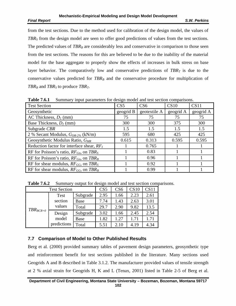
Mechanistic-Empirical Modeling and Design Model Development Final Report S.W. Perkins
Department of Civil Engineering, Montana State University – Bozeman, Bozeman, Montana 59717 102
from the test sections. Due to the method used for calibration of the design model, the values of
TBRS from the design model are seen to offer good predictions of values from the test sections.
The predicted values of TBRB are considerably less and conservative in comparison to those seen
from the test sections. The reasons for this are believed to be due to the inability of the material
model for the base aggregate to properly show the effects of increases in bulk stress on base
layer behavior. The comparatively low and conservative predictions of TBRT is due to the
conservative values predicted for TBRB and the conservative procedure for multiplication of
TBRB and TBRS to produce TBRT.
Table 7.6.1 Summary input parameters for design model and test section comparisons. Test Section CS5 CS6 CS10 CS11 Geosynthetic geogrid B geotextile A geogrid A geogrid A AC Thickness, D1 (mm) 75 75 75 75 Base Thickness, D2 (mm) 300 300 375 300 Subgrade CBR 1.5 1.5 1.5 1.5 2 % Secant Modulus, GSM-2% (kN/m) 595 680 425 425 Geosynthetic Modulus Ratio, GMR 0.615 0.313 0.595 0.595 Reduction factor for interface shear, RFI 1 0.765 1 1 RF for Poisson’s ratio, RFGν, on TBRS 1 0.83 1 1 RF for Poisson’s ratio, RFGν, on TBRB 1 0.96 1 1 RF for shear modulus, RFGG, on TBRS 1 0.92 1 1 RF for shear modulus, RFGG, on TBRB 1 0.99 1 1
Table 7.6.2 Summary output for design model and test section comparisons. Test Section CS5 CS6 CS10 CS11
Subgrade 2.95 1.66 2.23 2.61 Base 7.74 1.43 2.63 3.01
Test section values Total 29.7 2.90 9.82 13.5
Subgrade 3.02 1.66 2.45 2.54 Base 1.82 1.27 1.71 1.71
TBRBCR=0 Design model
predictions Total 5.51 2.10 4.19 4.34
7.7 Comparison of Model to Other Published Results
Berg et al. (2000) provided summary tables of pavement design parameters, geosynthetic type
and reinforcement benefit for test sections published in the literature. Many sections used
Geogrids A and B described in Table 3.1.2. The manufacturer provided values of tensile strength
at 2 % axial strain for Geogrids H, K and L (Tenax, 2001) listed in Table 2-5 of Berg et al.

Mechanistic-Empirical Modeling and Design Model Development Final Report S.W. Perkins
Department of Civil Engineering, Montana State University – Bozeman, Bozeman, Montana 59717 103
(2000). Values of other model parameters for this material are as assumed in Table 7.7.1. These
conditions were input into the design model to provide a comparison of predicted reinforcement
benefit. The studies described in Berg et al. (2000) listed either a total TBR or total BCR for
reinforcement benefit. As such, these corresponding numbers from the model are used as
comparison
In general, the predicted values of benefit from the model are seen to be conservative with
respect to those observed from the test sections. The cases where the model over predicted
results appear to be mostly from the studies of Barksdale et al. (1989) and Collin et al. (1996).
The study of Barksdale et al. (1989) used a relatively light wheel load (6.6 kN) and may be partly
responsible for the lack of benefit seen for this test section. The wheel load in the study of Collin
et al. (1996) was 20 kN and is also relatively light in comparison to that assumed in the design
model. The design model appears to be not as sensitive to base aggregate thickness as the results
from Collin et al. (1996) and Kinney et al. (1998) suggest.
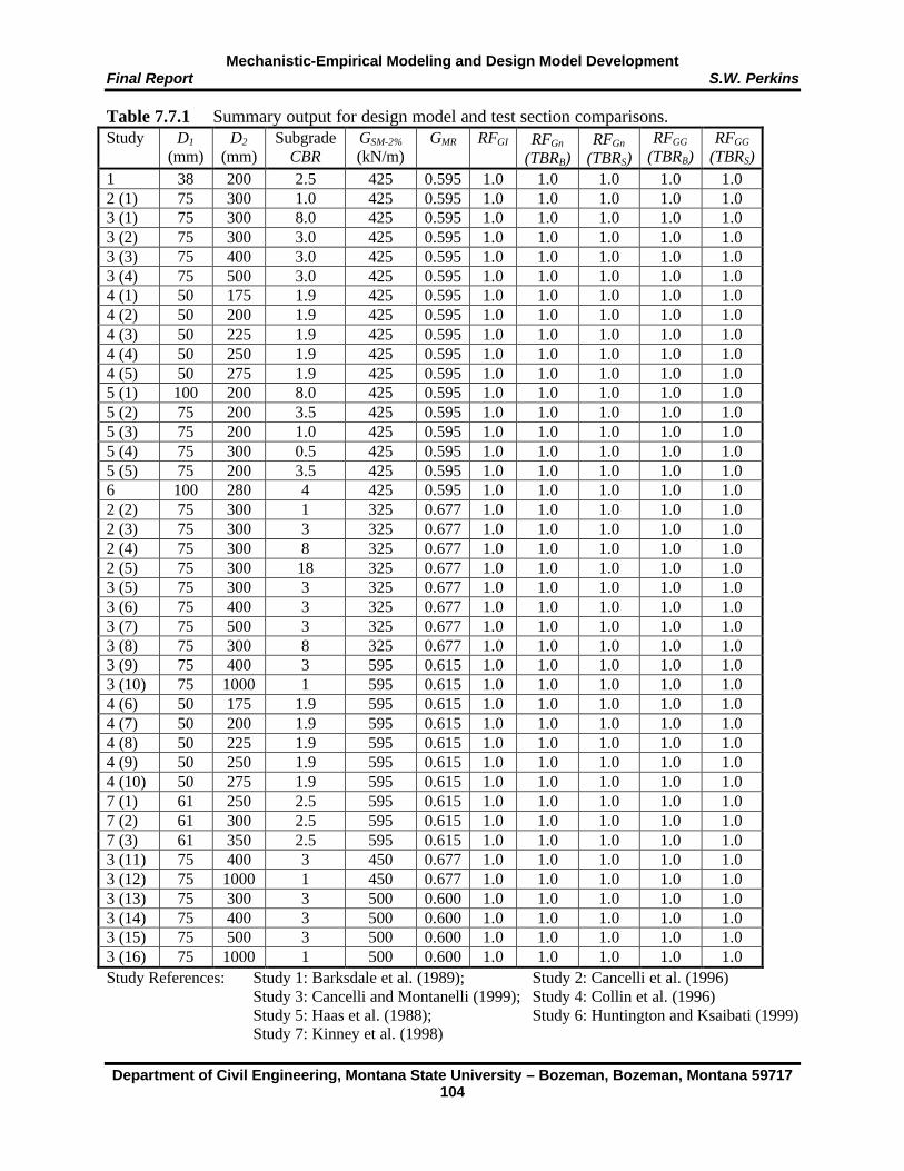
Mechanistic-Empirical Modeling and Design Model Development Final Report S.W. Perkins
Department of Civil Engineering, Montana State University – Bozeman, Bozeman, Montana 59717 104
Table 7.7.1 Summary output for design model and test section comparisons. Study D1
(mm) D2
(mm) Subgrade
CBR GSM-2% (kN/m)
GMR RFGI RFGν (TBRB)
RFGν (TBRS)
RFGG (TBRB)
RFGG (TBRS)
1 38 200 2.5 425 0.595 1.0 1.0 1.0 1.0 1.0 2 (1) 75 300 1.0 425 0.595 1.0 1.0 1.0 1.0 1.0 3 (1) 75 300 8.0 425 0.595 1.0 1.0 1.0 1.0 1.0 3 (2) 75 300 3.0 425 0.595 1.0 1.0 1.0 1.0 1.0 3 (3) 75 400 3.0 425 0.595 1.0 1.0 1.0 1.0 1.0 3 (4) 75 500 3.0 425 0.595 1.0 1.0 1.0 1.0 1.0 4 (1) 50 175 1.9 425 0.595 1.0 1.0 1.0 1.0 1.0 4 (2) 50 200 1.9 425 0.595 1.0 1.0 1.0 1.0 1.0 4 (3) 50 225 1.9 425 0.595 1.0 1.0 1.0 1.0 1.0 4 (4) 50 250 1.9 425 0.595 1.0 1.0 1.0 1.0 1.0 4 (5) 50 275 1.9 425 0.595 1.0 1.0 1.0 1.0 1.0 5 (1) 100 200 8.0 425 0.595 1.0 1.0 1.0 1.0 1.0 5 (2) 75 200 3.5 425 0.595 1.0 1.0 1.0 1.0 1.0 5 (3) 75 200 1.0 425 0.595 1.0 1.0 1.0 1.0 1.0 5 (4) 75 300 0.5 425 0.595 1.0 1.0 1.0 1.0 1.0 5 (5) 75 200 3.5 425 0.595 1.0 1.0 1.0 1.0 1.0 6 100 280 4 425 0.595 1.0 1.0 1.0 1.0 1.0 2 (2) 75 300 1 325 0.677 1.0 1.0 1.0 1.0 1.0 2 (3) 75 300 3 325 0.677 1.0 1.0 1.0 1.0 1.0 2 (4) 75 300 8 325 0.677 1.0 1.0 1.0 1.0 1.0 2 (5) 75 300 18 325 0.677 1.0 1.0 1.0 1.0 1.0 3 (5) 75 300 3 325 0.677 1.0 1.0 1.0 1.0 1.0 3 (6) 75 400 3 325 0.677 1.0 1.0 1.0 1.0 1.0 3 (7) 75 500 3 325 0.677 1.0 1.0 1.0 1.0 1.0 3 (8) 75 300 8 325 0.677 1.0 1.0 1.0 1.0 1.0 3 (9) 75 400 3 595 0.615 1.0 1.0 1.0 1.0 1.0 3 (10) 75 1000 1 595 0.615 1.0 1.0 1.0 1.0 1.0 4 (6) 50 175 1.9 595 0.615 1.0 1.0 1.0 1.0 1.0 4 (7) 50 200 1.9 595 0.615 1.0 1.0 1.0 1.0 1.0 4 (8) 50 225 1.9 595 0.615 1.0 1.0 1.0 1.0 1.0 4 (9) 50 250 1.9 595 0.615 1.0 1.0 1.0 1.0 1.0 4 (10) 50 275 1.9 595 0.615 1.0 1.0 1.0 1.0 1.0 7 (1) 61 250 2.5 595 0.615 1.0 1.0 1.0 1.0 1.0 7 (2) 61 300 2.5 595 0.615 1.0 1.0 1.0 1.0 1.0 7 (3) 61 350 2.5 595 0.615 1.0 1.0 1.0 1.0 1.0 3 (11) 75 400 3 450 0.677 1.0 1.0 1.0 1.0 1.0 3 (12) 75 1000 1 450 0.677 1.0 1.0 1.0 1.0 1.0 3 (13) 75 300 3 500 0.600 1.0 1.0 1.0 1.0 1.0 3 (14) 75 400 3 500 0.600 1.0 1.0 1.0 1.0 1.0 3 (15) 75 500 3 500 0.600 1.0 1.0 1.0 1.0 1.0 3 (16) 75 1000 1 500 0.600 1.0 1.0 1.0 1.0 1.0 Study References: Study 1: Barksdale et al. (1989); Study 2: Cancelli et al. (1996)
Study 3: Cancelli and Montanelli (1999); Study 4: Collin et al. (1996) Study 5: Haas et al. (1988); Study 6: Huntington and Ksaibati (1999) Study 7: Kinney et al. (1998)

Mechanistic-Empirical Modeling and Design Model Development Final Report S.W. Perkins
Department of Civil Engineering, Montana State University – Bozeman, Bozeman, Montana 59717 105
Table 7.7.2 Summary output for design model and test section comparisons. Study TBRT
Study TBRT Model
BCRT Study
BCRT Model
1 1.0 3.3 NA NA 2 (1) 17 6.8 NA NA 3 (1) 1.2 1.2 NA NA 3 (2) 220 2.2 NA NA 3 (3) 340 2.1 NA NA 3 (4) 8.4 1.9 NA NA 4 (1) 1.7 4.2 NA NA 4 (2) 1.8 4.1 NA NA 4 (3) 1.7 4.1 NA NA 4 (4) 3.3 4.0 NA NA 4 (5) 2.6 4.0 NA NA 5 (1) 3.3 1.1 NA NA 5 (2) 3.0 2.0 NA NA 5 (3) 1.8 7.2 NA NA 5 (4) 0.8 15.2 NA NA 5 (5) NA NA 50 20
6 NA NA 35 14 2 (2) 15 5.9 NA NA 2 (3) 5.2 2.0 NA NA 2 (4) 3.2 1.1 NA NA 2 (5) 4.5 1.0 NA NA 3 (5) 300 2.0 NA NA 3 (6) 330 1.9 NA NA 3 (7) 13 1.8 NA NA 3 (8) 1.6 1.1 NA NA 3 (9) 410 2.5 NA NA
3 (10) NA NA < 50 11 4 (6) 2.1 4.9 NA NA 4 (7) 2.8 4.9 NA NA 4 (8) 6.1 4.8 NA NA 4 (9) 10.0 4.8 NA NA
4 (10) 3.2 4.8 NA NA 7 (1) 10 3.4 NA NA 7 (2) 4.8 3.4 NA NA 7 (3) 2.0 3.3 NA NA
3 (11) 410 2.2 NA NA 3 (12) NA NA > 50 10 3 (13) 250 2.4 NA NA 3 (14) 670 2.3 NA NA 3 (15) 13 2.0 NA NA 3 (16) NA NA > 50 10
Mechanistic-Empirical Modeling and Design Model Development Final Report S.W. Perkins
Department of Civil Engineering, Montana State University – Bozeman, Bozeman, Montana 59717 106
7.8 Discussion of Design Model
The design model developed and presented in Section 7 and summarized in Section 8 is capable
of describing general trends relating reinforcement benefit to pavement design variables that
have previously been identified as having a significant impact on reinforced pavement
performance. In particular, the model is capable of showing that reinforcement benefit increases
with decreasing subgrade strength/stiffness, increasing geosynthetic modulus and is related to the
pavement structural thickness.
The model is expressed in terms of easily identifiable and well-recognized parameters
related to the pavement structure and the subgrade condition. Geosynthetic tensile modulus and
the ratio of modulus for the weak and strong directions of the material are determined from wide-
width tension tests (ASTM 4595). Reduction factors for other geosynthetic properties used in the
model, namely Poisson’s ratio and shear modulus, and for interface shearing resistance have
been developed for the geosynthetics used in test sections from which the model was calibrated.
These values provide initial guidance for selection of these reduction factors for other
geosynthetic types. Results from test sections using a wider range of geosynthetic products and
results from additional laboratory interface and tension tests are needed to further define these
reduction factors. In the absence of this information, the values provided in this report along with
general application guidelines provided in Berg et al. (2000) should be used for selection of these
factors.
The model presents a means of calculating reinforcement benefit for reinforcement effects
on the subgrade, the base aggregate or the total system. Equations for calculating benefit due to
each effect are provided and allow pavement designers to use their discretion in choosing which
effect or effects to design for.
The model is believed to be conservative on several accounts. Use of only benefit
accounting for effects in the subgrade layer results in a conservative design since effects in the
base layer are ignored. Comparisons of the model to test section results indicate that partial
benefits for reinforcement effects in the subgrade are considerably less than that for the entire
system. The method used to calculate reinforcement benefit for the base aggregate layer was
shown to yield values of benefit that are consistently less than those determined for test sections.
The equation used to calculate total TBR from the partial values for the base and subgrade layers
was shown to be conservative as compared to test section results. Given these observations, it is
Mechanistic-Empirical Modeling and Design Model Development Final Report S.W. Perkins
Department of Civil Engineering, Montana State University – Bozeman, Bozeman, Montana 59717 107
recommended that total values of TBR be used for design purposes. Finally, the method used to
calculate BCR and TBR/BCR combinations was shown to be conservative with respect to that
predicted by the finite element model.
The design model is based on certain conditions to which the model should be limited. The
response measures extracted from the finite element model are used to define pavement
performance in terms of permanent surface deformation or rutting. Furthermore, the design
model has been calibrated against test section results where pavement life was defined in terms
of rutting due to the accumulation of permanent strain in the base and subgrade layers. As such,
the model specifically addresses designs for which rutting is the controlling pavement distress
feature. It should be noted, however, that test sections have shown that the dynamic deflection of
the pavement surface is decreased by the use of reinforcement, which suggests that dynamic
tensile strain in the bottom of the asphalt concrete layer is reduced and fatigue life is increased.
The distress feature of rutting generally controls for pavement cross sections containing
relatively thin layers of asphalt concrete and base course aggregate and for pavement structural
layers resting on weak subgrade. The design model predicts the greatest levels of benefit for
those situations, meaning that the design model will tend to predict useful levels of benefit for
pavement designs for which rutting controls. The AASHTO ’93 pavement design guide does not
provide specific design checks for the individual pavement distress features of rutting and
asphalt fatigue cracking. Rather, designs developed using the AASHTO ’93 guide assume that
both pavement distress features are adequately addressed. For pavement designers who use
methods for individually checking rutting and fatigue cracking criteria (namely mechanistic-
empirical approaches), a method is presented in Section 8.7 to evaluate the effective increase in
resilient modulus of the base aggregate layer with reinforcement. This increased modulus should
be used to evaluate the fatigue cracking criteria for the asphalt concrete layer.
The design model was based on the results of finite element analyses calibrated against test
section results. The parametric study using the finite element response model employed a range
of input variables to which the design model should be limited. Furthermore, the regression
equations developed from the results of the parametric study contain certain limitations on the
range of values for input parameters. A summary of the permissible range of design model input
parameters is as follows:
1. 50 mm = D1 = 150 mm

Mechanistic-Empirical Modeling and Design Model Development Final Report S.W. Perkins
Department of Civil Engineering, Montana State University – Bozeman, Bozeman, Montana 59717 108
2. 150 mm = D2 = 600 mm
3. 0.5 = Subgrade CBR = 15 or 5.2 MPa = MS = 155 MPa
4. 33 kN/m = GSM-2% = 2000 kN/m
As discussed in Section 7.1.2, it is recommended that values of BCR > 0 be used only for
subgrades with a CBR = 1.0 (or MS = 10.3 MPa).
The finite element response model was used to evaluate cases only where the geosynthetic
was placed at the bottom of the base aggregate layer. Guidance for evaluation of benefit when
the geosynthetic is placed up within the base for thick base layer designs has not been provided.
The finite element models developed did not contain a subbase aggregate layer. For designs
using a subbase layer, recommendations are provided in Section 8.6 for accounting for this layer.
The model is based on results from a finite element model where pavement load has been
simulated by the application of a 40 kN load applied over a circular plate. Experimental test
section results from which the model has been validated used a similar load. The design model is
therefore designed to describe reinforcement benefit for conventional roadway applications
where the pavement load can be approximated in terms of a standard axle wheel load. The model
may not be appropriate for either lightly loaded traffic or for excessively loaded traffic.
The model is calibrated largely from results based on a permanent pavement surface
deformation of 12.5 mm. It is anticipated that roadways that can be designed for a rut depth
greater than 12.5 mm will realize reinforcement benefits greater than those predicted from this
model, meaning that this model should be conservative for roadways designed for a rut depth in
excess of 12.5 mm.
The model is based on asphalt concrete and base aggregate properties that correspond to
structural layer coefficients of approximately 0.4 and 0.14, respectively. To account for
pavement designs with different materials yielding different layer coefficients, recommendations
are provided in Section 8.5.
8.0 DESIGN MODEL SUMMARY
Section 7 described the methods used to interpret the data from the parametric study described in
Section 6. Through this interpretation process, a design model emerged and was compared to
results from test sections described in Section 3 and validated against others given in Berg et al.

Mechanistic-Empirical Modeling and Design Model Development Final Report S.W. Perkins
Department of Civil Engineering, Montana State University – Bozeman, Bozeman, Montana 59717 109
02.0%2
%2
TG sm =−
(2000). The purpose of this section is to summarize the essential elements of the design model
from that which was given in Section 7.
8.1 Design Inputs
The inputs to the design model are given in Table 8.1.1. The use of parameters D3, a1, a2, a3, m2
and m3 are introduced in Sections 8.5 and 8.6. Values of D1 and D2 should come from the design
of the unreinforced pavement for the project. The subgrade CBR used should be the design value
for the project. If some other subgrade property is given as the design value for the project
(resilient modulus, R-value, subgrade support value, etc.) this value should be correlated to CBR
through existing correlation equations such as Equation 4.2.9 relating CBR to resilient modulus.
A value for GSM-2% should be determined from test ASTM D 4595 (ASTM, 2001a). The secant
tensile modulus should be computed from the tensile strength at 2 % axial strain (T2%) from
Equation 8.1.1 and should represent the maximum value for either the machine or cross-machine
direction of the material. Reduction factors for geosynthetic interface shearing resistance should
be less than or equal to one. Reduction factors for geosynthetic Poisson’s ratio and shear
modulus should be either 1 or the values listed in Table 8.1.2.
(8.1.1)
Values of RFGI were calibrated as 1.0 for Geogrid A and B and as 0.765 for the Geotextile
listed in Table 3.1.2. Values of RFGν and RFGG were calibrated as 1.0 for Geogrid A and B, while
the values listed in Table 8.1.2 were used for the Geotextile. These values resulted from the
design model calibration work described in Section 7.6. Selection of values for these factors for
other geosynthetic products should be based on the values used here with assistance from the
application guidelines given in Berg et al. (2000).
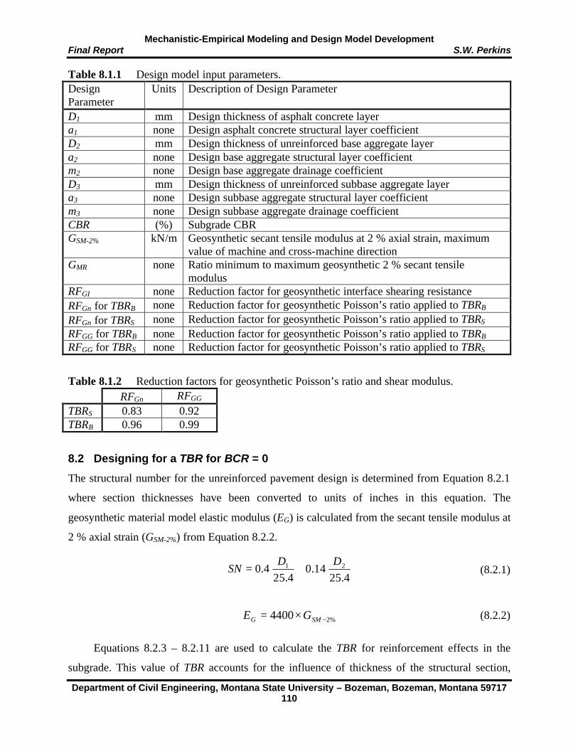
Mechanistic-Empirical Modeling and Design Model Development Final Report S.W. Perkins
Department of Civil Engineering, Montana State University – Bozeman, Bozeman, Montana 59717 110
4.2514.0
4.254.0 21 DD
SN +=
%24400 −×= SMG GE
Table 8.1.1 Design model input parameters. Design Parameter
Units Description of Design Parameter
D1 mm Design thickness of asphalt concrete layer a1 none Design asphalt concrete structural layer coefficient D2 mm Design thickness of unreinforced base aggregate layer a2 none Design base aggregate structural layer coefficient m2 none Design base aggregate drainage coefficient D3 mm Design thickness of unreinforced subbase aggregate layer a3 none Design subbase aggregate structural layer coefficient m3 none Design subbase aggregate drainage coefficient CBR (%) Subgrade CBR GSM-2% kN/m Geosynthetic secant tensile modulus at 2 % axial strain, maximum
value of machine and cross-machine direction GMR none Ratio minimum to maximum geosynthetic 2 % secant tensile
modulus RFGI none Reduction factor for geosynthetic interface shearing resistance RFGν for TBRB none Reduction factor for geosynthetic Poisson’s ratio applied to TBRB RFGν for TBRS none Reduction factor for geosynthetic Poisson’s ratio applied to TBRS RFGG for TBRB none Reduction factor for geosynthetic Poisson’s ratio applied to TBRB RFGG for TBRS none Reduction factor for geosynthetic Poisson’s ratio applied to TBRS
Table 8.1.2 Reduction factors for geosynthetic Poisson’s ratio and shear modulus. RFGν RFGG TBRS 0.83 0.92 TBRB 0.96 0.99
8.2 Designing for a TBR for BCR = 0
The structural number for the unreinforced pavement design is determined from Equation 8.2.1
where section thicknesses have been converted to units of inches in this equation. The
geosynthetic material model elastic modulus (EG) is calculated from the secant tensile modulus at
2 % axial strain (GSM-2%) from Equation 8.2.2.
(8.2.1)
(8.2.2)
Equations 8.2.3 – 8.2.11 are used to calculate the TBR for reinforcement effects in the
subgrade. This value of TBR accounts for the influence of thickness of the structural section,

Mechanistic-Empirical Modeling and Design Model Development Final Report S.W. Perkins
Department of Civil Engineering, Montana State University – Bozeman, Bozeman, Montana 59717 111
)log( 11103.36.1 oySNmGMSTBRSN +
− =≤≤
7.1
log1
2
1GM
GM
yy
m −
−
=
)6.1(1
1 110 mGM
oy
y −=
)log( 22100.63.3 oySNmGMSTBRSN +
− =≤≤
3.3log
)1(
22 −
−=
=
−
−GMSTBR
GM
SNy
m
)3.3(2
2 210 mGM
oy
y −=
( ) ( ) 1110100log8.49 )log8(log
1 +−= −−
CBRGGM
Ey
( ) ( ) 1110100
1057.1log108.1 )log7.1100(log66
2 +−×+×= −−−
−CBR
GGM ECBRy
0504.0028.01 )28.0(54.2 GTBR ECBRSN
GMS−==−
strength/stiffness of the subgrade and the value for the geosynthetic secant tensile modulus.
Depending on the value of SN from Equation 8.2.1, either Equation 8.2.6 or 8.2.9 is used to
calculate TBRS-GM. The model has not been validated for values of SN # 1.6 or $ 6.0. Computed
values of y1-GM less than one should be assigned a value of one. Similarly, computed values of
TBRS-GM less than one should be taken as one.
(8.2.3)
(8.2.4)
(8.2.5)
(8.2.6)
(8.2.7)
(8.2.8)
(8.2.9)
(8.2.10)
(8.2.11)
Equation 8.2.12 is used to calculate the TBR for reinforcement effects in the base. This
value of TBR accounts for the influence of thickness of the structural section, strength/stiffness
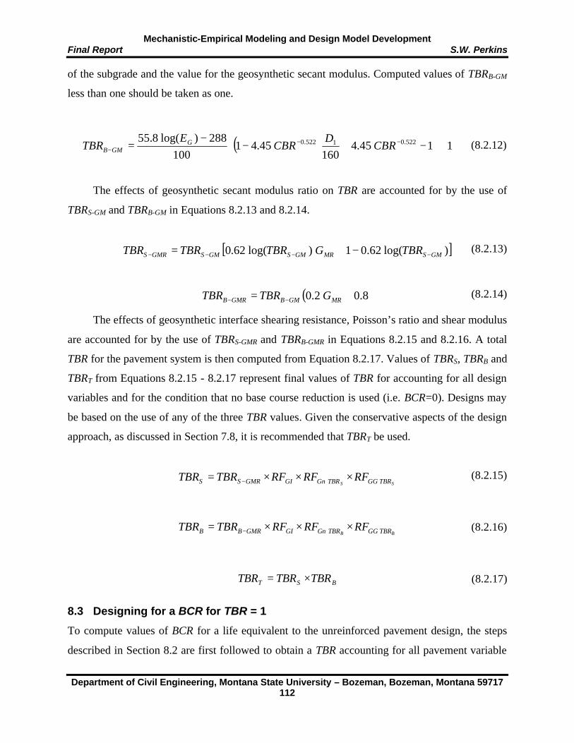
Mechanistic-Empirical Modeling and Design Model Development Final Report S.W. Perkins
Department of Civil Engineering, Montana State University – Bozeman, Bozeman, Montana 59717 112
( ) 1145.4160
45.41100
288)log(8.55 522.01522.0 +
−+−
−= −−
− CBRD
CBRE
TBR GGMB
[ ])log(62.01)log(62.0 GMSMRGMSGMSGMRS TBRGTBRTBRTBR −−−− −+=
( )8.02.0 += −− MRGMBGMRB GTBRTBR
BB TBRGGTBRGGIGMRBB RFRFRFTBRTBR ×××= − ν
SS TBRGGTBRGGIGMRSS RFRFRFTBRTBR ×××= − ν
BST TBRTBRTBR ×=
of the subgrade and the value for the geosynthetic secant modulus. Computed values of TBRB-GM
less than one should be taken as one.
(8.2.12)
The effects of geosynthetic secant modulus ratio on TBR are accounted for by the use of
TBRS-GM and TBRB-GM in Equations 8.2.13 and 8.2.14.
(8.2.13)
(8.2.14)
The effects of geosynthetic interface shearing resistance, Poisson’s ratio and shear modulus
are accounted for by the use of TBRS-GMR and TBRB-GMR in Equations 8.2.15 and 8.2.16. A total
TBR for the pavement system is then computed from Equation 8.2.17. Values of TBRS, TBRB and
TBRT from Equations 8.2.15 - 8.2.17 represent final values of TBR for accounting for all design
variables and for the condition that no base course reduction is used (i.e. BCR=0). Designs may
be based on the use of any of the three TBR values. Given the conservative aspects of the design
approach, as discussed in Section 7.8, it is recommended that TBRT be used.
(8.2.15)
(8.2.16)
(8.2.17)
8.3 Designing for a BCR for TBR = 1
To compute values of BCR for a life equivalent to the unreinforced pavement design, the steps
described in Section 8.2 are first followed to obtain a TBR accounting for all pavement variable

Mechanistic-Empirical Modeling and Design Model Development Final Report S.W. Perkins
Department of Civil Engineering, Montana State University – Bozeman, Bozeman, Montana 59717 113
4.2514.0
4.254.0 21 DD
SN +=
CBRM S ×= 1500
TBRWW UR −− = 1818
22
112 ma
DaSND
R
UR
−−
−=
effects. A TBRS, TBRB or TBRT may be used for design and as input to the remaining design steps
described below.
Equations 8.3.1 - 8.3.3 are used to calculate the number of ESAL’s for the unreinforced
pavement design. In this equation, certain values have been assumed for parameters in the
AASHTO 1993 pavement design equation. Since the design model has been calibrated against
these assumed values, the equation should be used as given.
(8.3.1)
(8.3.2)
(8.3.3)
With the design value of TBRS, TBRB or TBRT selected from the computations performed in
Section 8.2, a value for W18-R is computed from Equation 8.3.4.
(8.3.4)
The value of W18-R from Equation 8.3.4 is then used in Equation 8.3.1 to calculate a value of SN
for the reinforced pavement, with this value used in Equation 8.3.2 to determine a new value of
a2 for the reinforced pavement, with all other parameters in Equations 8.3.1 and 8.3.2 being
equal to those used for the unreinforced pavement. This calculation requires an iterative solution
for SN in Equation 8.3.1. Once a value of a2 for the reinforced pavement is obtained (a2-R), this
value is used in Equation 8.3.2 along with a reduced base thickness for the reinforced pavement
(D2-R) such that a SN identical to the unreinforced pavement is obtained. The reduced base
thickness is calculated from
(8.3.5)
( )
( )
−+
++
−+=− 84575.8)log(32.2
11094
4.0
15261.01log36.9^10
19.5
18 SU M
SN
SNW
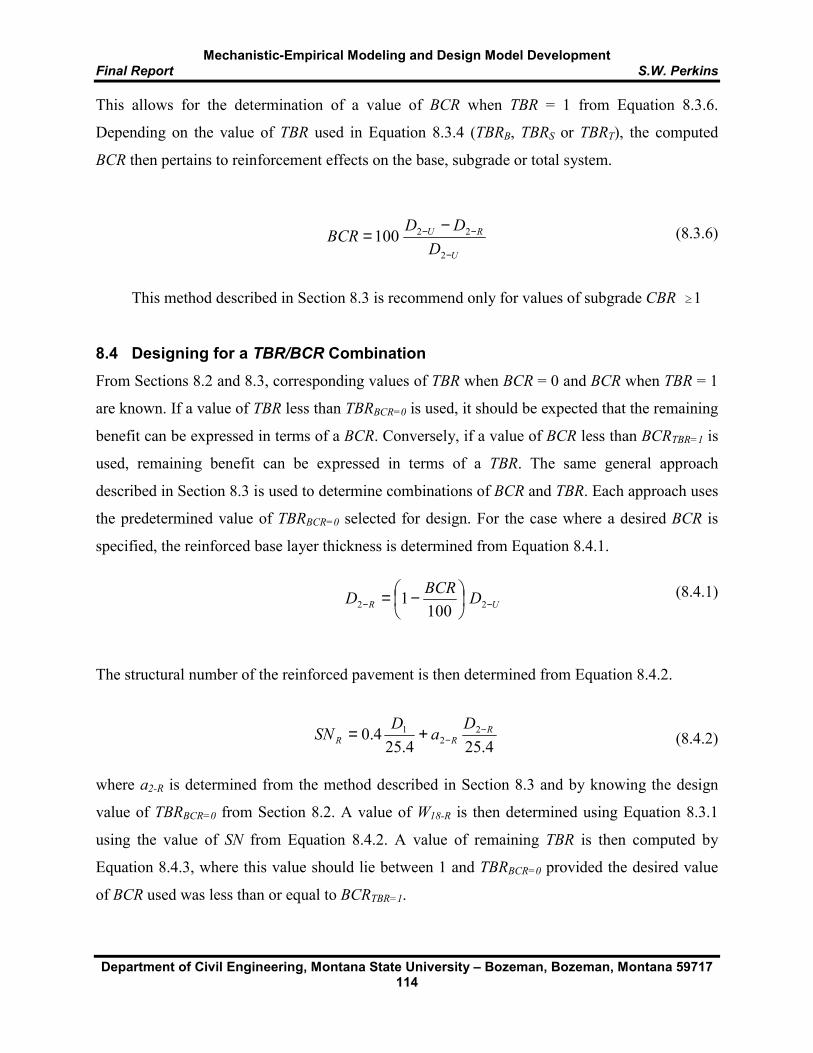
Mechanistic-Empirical Modeling and Design Model Development Final Report S.W. Perkins
Department of Civil Engineering, Montana State University – Bozeman, Bozeman, Montana 59717 114
U
RU
DDD
BCR−
−− −=
2
22100
UR DBCRD −−
−= 22 1001
4.254.254.0 2
21 R
RRD
aD
SN −−+=
This allows for the determination of a value of BCR when TBR = 1 from Equation 8.3.6.
Depending on the value of TBR used in Equation 8.3.4 (TBRB, TBRS or TBRT), the computed
BCR then pertains to reinforcement effects on the base, subgrade or total system.
(8.3.6)
This method described in Section 8.3 is recommend only for values of subgrade CBR $1
8.4 Designing for a TBR/BCR Combination
From Sections 8.2 and 8.3, corresponding values of TBR when BCR = 0 and BCR when TBR = 1
are known. If a value of TBR less than TBRBCR=0 is used, it should be expected that the remaining
benefit can be expressed in terms of a BCR. Conversely, if a value of BCR less than BCRTBR=1 is
used, remaining benefit can be expressed in terms of a TBR. The same general approach
described in Section 8.3 is used to determine combinations of BCR and TBR. Each approach uses
the predetermined value of TBRBCR=0 selected for design. For the case where a desired BCR is
specified, the reinforced base layer thickness is determined from Equation 8.4.1.
(8.4.1)
The structural number of the reinforced pavement is then determined from Equation 8.4.2.
(8.4.2)
where a2-R is determined from the method described in Section 8.3 and by knowing the design
value of TBRBCR=0 from Section 8.2. A value of W18-R is then determined using Equation 8.3.1
using the value of SN from Equation 8.4.2. A value of remaining TBR is then computed by
Equation 8.4.3, where this value should lie between 1 and TBRBCR=0 provided the desired value
of BCR used was less than or equal to BCRTBR=1.

Mechanistic-Empirical Modeling and Design Model Development Final Report S.W. Perkins
Department of Civil Engineering, Montana State University – Bozeman, Bozeman, Montana 59717 115
U
R
WW
TBR−
−=18
18
22
112 ma
DaSND
R
RR
−−
−=
= −−− 4.0
111
dde
aDD
= −−−− 0.114.0
2222
ddde
maDD
(8.4.3)
For the case where a desired TBR is specified, Equation 8.3.4 is used to calculate the
number of ESAL’s required of the reinforced section. Equation 8.3.1 is then solved iteratively to
give the required SN for the reinforced section (SNR). Equation 8.4.5 is then used to determine
the base layer thickness necessary to produce this SN, where the reinforced structural base layer
coefficient is used in this equation.
(8.4.5)
The remaining BCR is then determined from Equation 8.3.6, where the value obtained should lie
between 0 and BCRTBR=1 provided the desired value of TBR was less than TBRBCR=0.
This method described in Section 8.4 is recommend only for values of subgrade CBR $1.
8.5 Adjustment of Structural Layer Coefficients
The material models used for the asphalt concrete and base aggregate layers were calibrated to
match the properties of these layers from test sections reported in Section 3 and were shown to
approximate layer coefficients of 0.4 and 0.14, respectively. Furthermore, a base aggregate
drainage layer coefficient (m2) of 1.0 was used for calibration of the model. To use the design
model developed in this project for designs involving material layers having other layer and
drainage coefficients, it is suggested that the design AC thickness (D1-d), design base aggregate
thickness (D2-d) be adjusted to equivalent values (D1-e, D2-e) using Equations 8.5.1 and 8.5.2,
where a1-d and a2-d are the design values for the layer coefficients and m2-d is the design value for
the drainage coefficient.
(8.5.1)
(8.5.2)

Mechanistic-Empirical Modeling and Design Model Development Final Report S.W. Perkins
Department of Civil Engineering, Montana State University – Bozeman, Bozeman, Montana 59717 116
= −−
−− 0.114.033
33dd
de
maDD
Equivalent values of layer thickness (D1-e, D2-e) are then used directly for D1 and D2 in all
equations given in Sections 8.1-8.4.
8.6 Accounting for Subbase Aggregate Layers
The finite element response models did not contain a subbase layer. For designs using a subbase
layer, and where the reinforcement will be placed at the bottom of the subbase, it is suggested
that the design layer thickness of the subbase (D3-d) be converted to an equivalent base aggregate
thickness (D3-e) having a structural layer coefficient of 0.14 and a drainage coefficient of 1.0 and
added to the base aggregate thickness (D2). The equivalent thickness can be calculated from
Equation 8.6.1, where a3-d is the design value of the structural coefficient for the subbase
aggregate layer and m3-d is the design value of the drainage coefficient for the subbase layer.
(8.6.1)
Designs using a subbase according to Equation 8.6.1 are valid only when the geosynthetic
is placed at the bottom of the subbase layer. Special attention should be given to the selection of
the reduction factor for geosynthetic interface shearing resistance (RGI) because of the typically
large particle sizes and lack of angularity associated with common subbase aggregate materials.
8.7 Evaluating Asphalt Fatigue Cracking Criteria
As discussed in Section 7.8, the design model is based on response measures extracted from the
finite element model used to define pavement performance in terms of permanent surface
deformation or rutting. The design model has been calibrated against test section results where
pavement life was defined in terms of rutting due to the accumulation of permanent strain in the
base and subgrade layers. As such, the model specifically addresses designs for which rutting is
the controlling pavement distress feature. It should be noted, however, that test sections have
shown that the dynamic deflection of the pavement surface is decreased by the use of
reinforcement, which suggests that dynamic tensile strain in the bottom of the asphalt concrete
layer is reduced and fatigue life is increased.
The distress feature of rutting generally controls for pavement cross sections containing
relatively thin layers of asphalt concrete and base course aggregate and for pavement structural
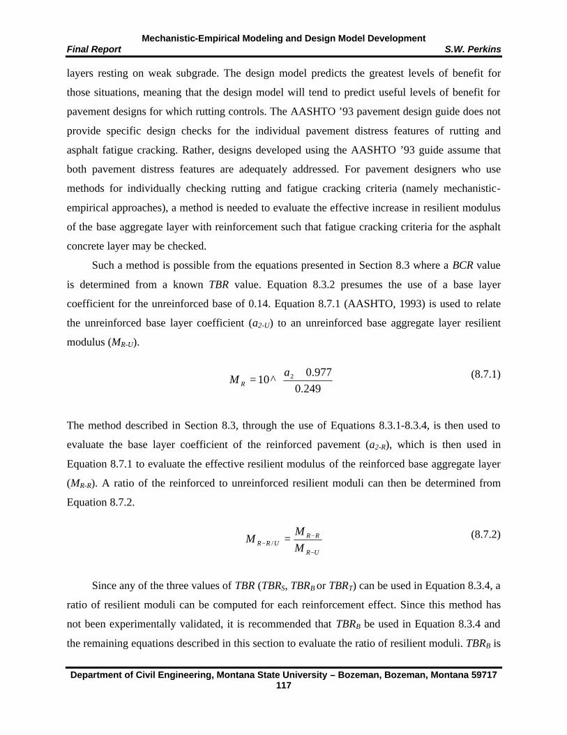
Mechanistic-Empirical Modeling and Design Model Development Final Report S.W. Perkins
Department of Civil Engineering, Montana State University – Bozeman, Bozeman, Montana 59717 117
+
=249.0
977.0^10 2a
M R
UR
RRURR M
MM
−
−− =/
layers resting on weak subgrade. The design model predicts the greatest levels of benefit for
those situations, meaning that the design model will tend to predict useful levels of benefit for
pavement designs for which rutting controls. The AASHTO ’93 pavement design guide does not
provide specific design checks for the individual pavement distress features of rutting and
asphalt fatigue cracking. Rather, designs developed using the AASHTO ’93 guide assume that
both pavement distress features are adequately addressed. For pavement designers who use
methods for individually checking rutting and fatigue cracking criteria (namely mechanistic-
empirical approaches), a method is needed to evaluate the effective increase in resilient modulus
of the base aggregate layer with reinforcement such that fatigue cracking criteria for the asphalt
concrete layer may be checked.
Such a method is possible from the equations presented in Section 8.3 where a BCR value
is determined from a known TBR value. Equation 8.3.2 presumes the use of a base layer
coefficient for the unreinforced base of 0.14. Equation 8.7.1 (AASHTO, 1993) is used to relate
the unreinforced base layer coefficient (a2-U) to an unreinforced base aggregate layer resilient
modulus (MR-U).
(8.7.1)
The method described in Section 8.3, through the use of Equations 8.3.1-8.3.4, is then used to
evaluate the base layer coefficient of the reinforced pavement (a2-R), which is then used in
Equation 8.7.1 to evaluate the effective resilient modulus of the reinforced base aggregate layer
(MR-R). A ratio of the reinforced to unreinforced resilient moduli can then be determined from
Equation 8.7.2.
(8.7.2)
Since any of the three values of TBR (TBRS, TBRB or TBRT) can be used in Equation 8.3.4, a
ratio of resilient moduli can be computed for each reinforcement effect. Since this method has
not been experimentally validated, it is recommended that TBRB be used in Equation 8.3.4 and
the remaining equations described in this section to evaluate the ratio of resilient moduli. TBRB is
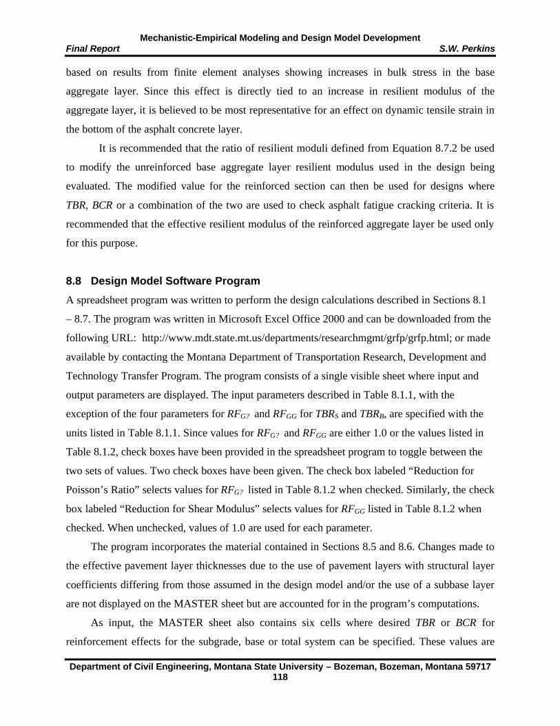
Mechanistic-Empirical Modeling and Design Model Development Final Report S.W. Perkins
Department of Civil Engineering, Montana State University – Bozeman, Bozeman, Montana 59717 118
based on results from finite element analyses showing increases in bulk stress in the base
aggregate layer. Since this effect is directly tied to an increase in resilient modulus of the
aggregate layer, it is believed to be most representative for an effect on dynamic tensile strain in
the bottom of the asphalt concrete layer.
It is recommended that the ratio of resilient moduli defined from Equation 8.7.2 be used
to modify the unreinforced base aggregate layer resilient modulus used in the design being
evaluated. The modified value for the reinforced section can then be used for designs where
TBR, BCR or a combination of the two are used to check asphalt fatigue cracking criteria. It is
recommended that the effective resilient modulus of the reinforced aggregate layer be used only
for this purpose.
8.8 Design Model Software Program
A spreadsheet program was written to perform the design calculations described in Sections 8.1
– 8.7. The program was written in Microsoft Excel Office 2000 and can be downloaded from the
following URL: http://www.mdt.state.mt.us/departments/researchmgmt/grfp/grfp.html; or made
available by contacting the Montana Department of Transportation Research, Development and
Technology Transfer Program. The program consists of a single visible sheet where input and
output parameters are displayed. The input parameters described in Table 8.1.1, with the
exception of the four parameters for RFG? and RFGG for TBRS and TBRB, are specified with the
units listed in Table 8.1.1. Since values for RFG? and RFGG are either 1.0 or the values listed in
Table 8.1.2, check boxes have been provided in the spreadsheet program to toggle between the
two sets of values. Two check boxes have been given. The check box labeled “Reduction for
Poisson’s Ratio” selects values for RFG? listed in Table 8.1.2 when checked. Similarly, the check
box labeled “Reduction for Shear Modulus” selects values for RFGG listed in Table 8.1.2 when
checked. When unchecked, values of 1.0 are used for each parameter.
The program incorporates the material contained in Sections 8.5 and 8.6. Changes made to
the effective pavement layer thicknesses due to the use of pavement layers with structural layer
coefficients differing from those assumed in the design model and/or the use of a subbase layer
are not displayed on the MASTER sheet but are accounted for in the program’s computations.
As input, the MASTER sheet also contains six cells where desired TBR or BCR for
reinforcement effects for the subgrade, base or total system can be specified. These values are

Mechanistic-Empirical Modeling and Design Model Development Final Report S.W. Perkins
Department of Civil Engineering, Montana State University – Bozeman, Bozeman, Montana 59717 119
specified when combinations of TBR/BCR are desired. Changing any of the input values or
options automatically causes the program to run and compute values listed in the output table.
Output consists of values for TBRBCR=0 and BCRTBR=1 for reinforcement effects in the
subgrade, base and total system. The designer may choose to use any of the three sets of values.
For the desired values of TBR and BCR listed as input, values of remaining TBR and BCR are
computed and listed as output. The output also contains computed values of effective base
aggregate resilient modulus ratio for evaluation of asphalt concrete fatigue cracking criteria as
described in Section 8.7. Limitations associated with the use of the model were discussed in
Section 7.8 and are presented again in Appendix B.
9.0 INCORPORATION OF DESIGN MODEL INTO A STANDARD OF PRACTICE
This report presents a design model for computing reinforcement benefit of geosynthetics used in
the base course of flexible pavements. Computed benefit is in terms of a TBR, BCR or
combination of the two. These values can be used directly in the recommended standard of
practice given by Berg et al. (2000). These values can be used to directly modify an unreinforced
pavement according to step 4 of the recommended standard of practice (see Section 2.3 of this
report). Further guidance is provided in Appendix B of this report. The example specification
provided in Berg et al. (2000) will require revisions to account for the design model proposed
herein. Lastly, the AASHTO Subcommittee on Materials Technical Section 4E, Task Force on
Geogrids/Geotextiles is encouraged to consider adoption of this design method into the existing
AASHTO Designation PP 46-01.
10.0 CONCLUSIONS
The work described in this report has resulted in the development of a generic design model for
geosynthetic reinforced flexible pavements. The model is expressed solely in terms of equations
relating reinforcement benefit to pavement and geosynthetic input design parameters. These
equations are based on the results of predictions of reinforcement benefit from a finite element
based mechanistic-empirical model from over 465 analyzed cases. The mechanistic-empirical
model and the design model were calibrated from test section results for reinforced pavements
presented in Perkins (1999a). The design model was further validated by comparison of

Mechanistic-Empirical Modeling and Design Model Development Final Report S.W. Perkins
Department of Civil Engineering, Montana State University – Bozeman, Bozeman, Montana 59717 120
predictions to values of benefit from other studies reported in the literature and summarized in
Berg et al. (2000).
The design model presents a means of calculating reinforcement benefit for reinforcement
effects on the subgrade, the base aggregate or both. Equations for calculating benefit due to each
effect are provided and allow pavement designers to use their discretion in choosing for which
effect to design.
The design model has been shown to be sensitive to pavement design variables that have
previously been identified as having a significant impact on reinforced pavement performance.
In particular, the model is capable of showing that reinforcement benefit increases with
decreasing subgrade strength/stiffness, increasing geosynthetic tensile modulus and is sensitive
to the pavement structural thickness. Furthermore, the model is shown to be sensitive to the ratio
of geosynthetic tensile modulus in the weak to strong directions of the material. The model is
calibrated from the use of geosynthetic secant tensile modulus values determined at 2 % axial
strain according to ASTM 4595 (ASTM, 2001a).
The design model attempts to account for geosynthetic properties pertinent to the type and
structure of the material through the assignment of reduction factors for geosynthetic material
Poisson’s ratio, shear modulus and geosynthetic/aggregate shear interaction. Geosynthetic
material Poisson’s ratio and shear modulus are parameters existing in the anisotropic elastic
material model used for the geosynthetic and were shown to have a moderate influence on
reinforcement benefit. Reduction factors for Poisson’s ratio and shear modulus correspond to one
of two values for either good or poor material property conditions and were calibrated for the
two types of geosynthetics used in test sections reported in Perkins (1999a). Similarly, the
reduction factor for interface shearing resistance was calibrated from these test section results.
These values serve as a starting point for selection of values for other geosynthetic types. In the
absence of additional results from test sections using a broader range of geosynthetic products,
judgment and experience are required for selection of final values for design.
The design model appears to yield mostly conservative predictions of reinforcement benefit
when compared to results available in the literature. Conservatism in the model results from
several sources. Use of only benefit accounting for effects in the subgrade layer would result in a
conservative design since effects in the base layer would be ignored. Comparisons of the model
to test section results indicate that partial benefits for reinforcement effects in the subgrade are

Mechanistic-Empirical Modeling and Design Model Development Final Report S.W. Perkins
Department of Civil Engineering, Montana State University – Bozeman, Bozeman, Montana 59717 121
considerably less than that for the entire system. The method used to calculate reinforcement
benefit for the base aggregate layer was shown to yield values of benefit that are consistently less
than those determined for test sections. The equation used to calculate total TBR from the partial
values for the base and subgrade layers was shown to be conservative as compared to test section
results. Finally the method used to calculate BCR and TBR/BCR combinations was shown to be
conservative with respect to that predicted by the finite element model. In spite of this inherent
conservatism, use of the model is shown to offer significant life-cycle cost benefits for several
pavement design examples illustrated in Appendix B.
The design model is based on certain conditions to which the model should be limited. The
model is based on results from a finite element model where pavement load has been simulated
by the application of a 40 kN load applied over a circular plate. Experimental test section results
from which the model has been validated used a similar load. The design model is therefore
designed to describe reinforcement benefit for conventional roadway applications where the
pavement load can be approximated in terms of a standard axle wheel load. The model may not
be appropriate for either lightly loaded traffic or for excessively loaded traffic.
The design model is calibrated largely from results based on a permanent pavement surface
deformation of 12.5 mm. It is anticipated that roadways that can be designed for a rut depth
greater than 12.5 mm will realize reinforcement benefits greater than those predicted from this
model, meaning that this model should be conservative for roadways designed for a rut depth in
excess of 12.5 mm.
The model is based on asphalt concrete and base aggregate properties that correspond to
structural layer coefficients of approximately 0.4 and 0.14, respectively. Recommendations were
provided to account for pavement designs with different materials yielding different layer
coefficients.
All cases of reinforcement were modeled by placement of the geosynthetic at the bottom of
the base aggregate layer. As such, the design model cannot account for situations where it might
be desirable to place the geosynthetic further up in the base aggregate layer. Work involving the
assessment of benefit for situations where the geosynthetic was elevated up into the base layer
was not performed because of the relatively low values of benefit that were derived for the base
aggregate layer. Reliable values of benefit for cases where the geosynthetic is elevated up into
Mechanistic-Empirical Modeling and Design Model Development Final Report S.W. Perkins
Department of Civil Engineering, Montana State University – Bozeman, Bozeman, Montana 59717 122
the base aggregate layer requires a material model for the base aggregate that is more suited for
demonstrating benefits observed in experimental test sections.
Values of reinforcement benefit from the design model can be used directly in a
recommended standard of practice for reinforced pavement design presented in Berg et al. (2000)
and AASHTO (2001). Appendix B of this report describes the steps necessary to carry out a
pavement design using geosynthetic reinforcement, where the material presented in this report
can be used in place of step 4 of the previously recommended standard of practice. The
AASHTO Subcommittee on Materials Technical Section 4E, Task Force on
Geogrids/Geotextiles is encouraged to consider adoption of this design method into the existing
AASHTO Designation PP 46-01.
Further work for improvement of the design model should focus on a better description of
reinforcement benefit for reinforcement effects in the base aggregate layer. The design model as
presented in this report yields conservative predictions of this reinforcement component.
Improvements in the material model used for the base aggregate layer would be required to
improve upon predictions of this component of benefit. These improvements would then also
warrant examining the model for predictions of benefit for cases where the geosynthetic is
moved up into the base aggregate layer. Further work should also be performed to allow
assignment of reduction factors for geosynthetic Poisson’s ratio, shear modulus and
geosynthetic/aggregate shear interaction to different geosynthetics types. Finally, future results
from new test sections should be used to further refine and update the model.
11.0 REFERENCES
AASHTO (2001), Recommended Practice for Geosynthetic Reinforcement of the Aggregate
Base Course of Flexible Pavement Structures, AASHTO Designation PP 46-01. AASHTO (1997a), Standard Specification for Geotextiles – M288, Standard Specifications for
Transportation Materials and Methods of Sampling and Testing, 18th Edition, American Association of State Highway and Transportation Officials, Washington, D.C., USA.
AASHTO (1997b), AASHTOWare DARWin 3.1, Pavement Design and Analysis System, American Association of State Highway and Transportation Officials, Washington, D.C., USA.
AASHTO (1993), AASHTO Guide for Design of Pavement Structures, American Association of State Highway and Transportation Officials, Washington, D.C., USA.
AASHTO (1991), “Standard Method of Test for Resilient Modulus of Subgrade Soils and Untreated Base/Subbase Materials”, AASHTO Designation T 292-91, Standard
Mechanistic-Empirical Modeling and Design Model Development Final Report S.W. Perkins
Department of Civil Engineering, Montana State University – Bozeman, Bozeman, Montana 59717 123
Specifications for Transportation Materials and Methods of Sampling and Testing, Part II, Methods of Sampling and Testing, American Association of State Highway and Transportation Officials, Washington, D.C., USA.
Allied Engineering (2000), Final Geotechnical Report, Rosebud County Line East Roadway Reconstruction, Montana Department of Transportation, Project Number STPP 14-6(8)207, Control Number 4060, Rosebud Country, Montana, Allied Engineering Services, Incorporated Project 99-048, Bozeman, MT, USA.
AMOCO (1996). Personal Fax Communication, 6-12-1996. AMOCO (2001). Personal Email Communication, 4-23-2001. Asphalt Institute (1991), Computer Program DAMA, Pavement Structural Analysis Using Multi-
Layered Elastic Theory, Asphalt Institute, Lexington, KY, USA. ASTM (2001a), Annual Book of ASTM Standards, Soil and Rock (II): D4943-Latest;
Geosynthetics, Vol. 04.09, Section 4, American Society of Testing and Materials, West Conshohocen, PA, USA.
ASTM (2001b), Annual Book of ASTM Standards, Road and Paving Materials; Vehicle Pavement Systems, Vol. 04.03, Section 4, American Society of Testing and Materials, West Conshohocen, PA, USA.
Barksdale, R.D., Brown, S.F. and Chan, F. (1989), “Potential Benefits of Geosynthetics in Flexible Pavement Systems”, National Cooperative Highway Research Program Report No. 315, Transportation Research Board, National Research Council, Washington DC.
Berg R.R., Christopher, B.R. and Perkins, S.W. (2000), Geosynthetic Reinforcement of the Aggregate Base Course of Flexible Pavement Structures, GMA White Paper II, Geosynthetic Materials Association, Roseville, MN, USA, 130p.
Burd, H.J. and Brocklehurst, C.J. (1992), “Parametric Studies of a Soil Reinforcement Problem Using Finite Element Analysis”, Proceedings of the Conference on Computer Methods and Advances in Geomechanics, Balkema, pp. 1783-1788.
Burd, H.J. and Brocklehurst, C.J. (1990), “Finite Element Studies of the Mechanics of Reinforced Unpaved Roads”, Proceedings of the 4th International Conference on Geotextiles, Geomembranes and Related Products, The Hauge, Netherlands, pp. 217-221.
Burd, H.J. and Houlsby, G.T. (1986), “A Large Strain Finite Element Formulation for One Dimensional Membrane Elements”, Computers and Geotechnics, Vol. 2, pp. 3-22.
Cancelli, A. and Montanelli, F. (1999), “In-Ground Test for Geosynthetic Reinforced Flexible Paved Roads”, Proceedings of the Conference Geosynthetics ’99, Boston, MA, USA, Vol. 2, pp. 863-878.
Cancelli, A., Montanelli, F., Rimoldi, P. and Zhao, A. (1996), “Full Scale Laboratory Testing on Geosynthetic Reinforced Paved Roads”, Proceedings of the International Symposium on Earth Reinforcement, Fukuoka/Kyushu, Japan, November, Balkema, pp. 573-578.
Chen, D.-H., Zaman, M., Laguros, J. and Soltani, A. (1995), “Assessment of Computer Programs for Analysis of Flexible Pavement Structure”, In Transportation Research Record 1482, TRB, National Research Council, Washington, DC, USA, pp. 123-133.
Christopher, B.R., Berg, R.R. and Perkins, S.W. (2001), Geosynthetic Reinforcements in Roadway Sections, NCHRP Synthesis for NCHRP Project 20-7, Task 112, Transportation Research Board, Washington, D.C., In-Print.
Colbond (1998), TRC-Grid, Design and Installation Guide, Akzo Nobel Geosynthetics, Arnhem, the Netherlands, 24p.

Mechanistic-Empirical Modeling and Design Model Development Final Report S.W. Perkins
Department of Civil Engineering, Montana State University – Bozeman, Bozeman, Montana 59717 124
Collin, J. G., Kinney, T. C. and Fu, X. (1996), “Full Scale Highway Load Test of Flexible Pavement Systems With Geogrid Reinforced Base Courses” Geosynthetics Intentional, Vol. 3, No. 4, pp. 537-549.
Dafalias, Y.F. and Hermann, L.R. (1986), “Bounding Surface Plasticity. II: Application to Isotropic Cohesive Soils”, Journal of Engineering Mechanics, ASCE, Vol. 112, No. 12, pp. 1263-1291.
Dafalias, Y.F. and Hermann, L.R. (1982), “Bounding Surface Formulation of Soil Plasticity”, Soil Mechanics-Transient and Cyclic Loads, Chapter 10, John Wiley and Sons, Ltd., pp. 253-282.
Dafalias, Y.F. (1975), On Cyclic and Anisotropic Plasticity, Ph.D. Thesis, University of California at Berkeley.
Davies, M.C.R. and Bridle, R.J. (1990), “Predicting the Permanent Deformation of Reinforced Flexible Pavement Subject to Repeated Loading,” Proceedings of the International Reinforced Soil Conference, Performance of Reinforced Soil Structures, Glasgow, UK, A. McGown, K.C. Yeo and K.Z. Andrawes, eds., British Geotechnical Society, Thomas Telford, London, pp. 421 - 425, UK.
Desai, C.S., Somasundaram, S. and Frantziskonis, G.N. (1986), “A Hierarchical Approach for Constitutive Modeling of Geologic Materials”, International Journal of Numerical Methods in Geomechanics, Vol. 10, pp.25-257.
Dondi, G. (1994), “Three-Dimensional Finite Element Analysis of a Reinforced Paved Road”, Proceedings of the Fifth International Conference on Geotextiles, Geomembranes and Related Products, Singapore, pp. 95-100.
Dorman, G.M. and Metcalf, C.T. (1965), “Design Curves for Flexible Pavements Based on Layered System Theory”, Highway Research Record 71, Highway Research Board, Washington, D.C. USA, pp. 69-84.
GRI (2001), GRI Test Methods and Standards, Geosynthetic Research Institute, Drexel University, Philadelphia, PA, USA.
Haas R., Wall, J. and Carroll, R.G. (1988), “Geogrid Reinforcement of Granular Bases in Flexible Pavements,” In Transportation Research Record 1188, TRB, National Research Council, Washington DC, USA, pp. 19 - 27.
Harichandran, R.S., Yeh, M.S. and Baladi, G.Y. (1989), MICH-PAVE User’s Manual, Final Report, FHWA-MI-RD-89-032, Department of Civil and Environmental Engineering, Michigan State University, East Lansing, MI, USA.
Heukelom, W. and Klomp, A.J.G. (1962), “Dynamic Testing as a Means of Controlling Pavements During and After Construction”, Proceedings of the First International Conference on the Structural Design of Asphalt Pavements, pp. 667-685.
Hibbitt, Karlson and Sorensen (1998), ABAQUS Standard User’s Manuals, Version 5.8, Pawtucket, RI, USA.
Holtz, R.D. and Kovacs, W.D. (1981), An Introduction to Geotechnical Engineering, Prentice Hall, Englewood Cliffs, NJ, USA., 733p.
Huang, Y.H. (1993), Pavement Analysis and Design, Prentice Hall, Englewood Cliffs, NJ, USA, 805p.
Huntington, G. and Ksaibati, K. (1999), “Evaluation of Geogrid-Reinforced Granular Base”, Geotechnical Special Publication No. 89, Recent Advances in the Characterization of Transportation Geo-Materials, ASCE, pp. 13-24.
IFAI (1994), 1995 Specifier’s Guide, Geotechnical Fabrics Report, Vol. 12, No. 9, pg. 169.
Mechanistic-Empirical Modeling and Design Model Development Final Report S.W. Perkins
Department of Civil Engineering, Montana State University – Bozeman, Bozeman, Montana 59717 125
ILLI-PAVE (1990), ILLI-PAVE PC Version User’s Manual, NCHRP 1-26, Transportation Faculties Group, University of Illinois at Urbana-Champaign.
Kaliakin, V.N., Dafalias, Y.F. and Hermann, L.R. (1987), Time Dependent Bounding Surface Model for Isotropic Cohesive Soils, notes for a short course held in conjunction with the Second International Conference on Constitutive Laws for Engineering Materials, Tucson, AZ, January.
Kinney, T.C., Abbott, J. and Schuler, J. (1998), “Benefits of Using Geogrids for Base Reinforcement with Regard to Rutting”, Transportation Research Record 1611, Transportation Research Board, National Research Council, Washington, DC, USA, pp. 86-96.
Kopperman, S.G., Tiller, and Tseng, M. (1986), ELSYM5, Interactive Microcomputer Version, User’s Manual, Report No. FHWA-TS-87-206, Federal Highway Administration, Washington, D.C., USA.
Liu, X., Scarpas, A., Blaauwendraad, J. and Genske, D.D. (1998), “Geogrid Reinforcing of Recycled Aggregate Materials for Road Construction”, 77th Annual Meeting of the Transportation Research Board, Preprint 981343, Washington, D. C.
Meyer, N. and Elias, J.M. (1999), “Design Methods for Roads Reinforced with Multifunctional Geogrids for Subbase Stabilization”, Translation of a paper in German presented at the German Conference on Geosynthetics, Kunststoffe in der Geotechnik, Technical University of Munich, March.
Mirafi (1982), Guidelines for Design of Flexible Pavements Using Mirafi Woven Geotextiles, TC Mirafi, Pendergrass, GA, USA, 23 p.
Miura, N., Sakai, A., Taesiri, Y., Yamanouchi, T. and Yasuhara, K. (1990), “Polymer Grid Reinforced Pavement on Soft Clay Grounds”, Geotextiles and Geomembranes, Vol. 9, pp. 99-123.
MDT (2001), Montana Department of Transportation Internet Resource, “MDT Contractor’s System”: http://www.mdt.state.mt.us/cntrct/contract.htm.
Penner, R., Haas, R., Walls, J. and Kennepohl, G. (1985), “Geogrid Reinforcement of Granular Bases”, Paper Presented at the Roads and Transportation Association of Canada Annual Conference, Vancouver, Canada, September.
Perkins, S.W. (2001a), Numerical Modeling of Geosynthetic Reinforced Flexible Pavements, Montana Department of Transportation, Helena, Montana, Report No. FHWA/MT-01/003/99160-2, 97p.
Perkins, S.W. (2001b), Mechanistic-Empirical Modeling and Design Model Development of Geosynthetic Reinforced Flexible Pavements: Appendix C - DARWin Output, Montana Department of Transportation, Helena, Montana, Report No. FHWA/MT-01/002/99160-1B, 89p.
Perkins, S.W. (1999a), Geosynthetic Reinforcement of Flexible Pavements: Laboratory Based Pavement Test Sections, Montana Department of Transportation, Helena, Montana, Report No. FHWA/MT-99/8106-1, 140 p.
Perkins, S.W. (1999b), “Mechanical Response of Geosynthetic-Reinforced Flexible Pavements”, Geosynthetics International, Vol. 6, No. 5, pp. 347-382.
Perkins, S.W., Ismeik M. and Fogelsong, M.L (1999), “Influence of Geosynthetic Placement Position on the Performance of Reinforced Flexible Pavement Systems”, Proceedings of the Conference Geosynthetics’99, Boston, MA, USA, V. 1, pp. 253-264.
Perkins, S.W., Ismeik, M., Fogelsong, M.L., Wang, Y. and Cuelho, E.V. (1998a), “Geosynthetic-

Mechanistic-Empirical Modeling and Design Model Development Final Report S.W. Perkins
Department of Civil Engineering, Montana State University – Bozeman, Bozeman, Montana 59717 126
Reinforced Pavements: Overview and Preliminary Results”, Proceedings of the Sixth International Conference on Geosynthetics, Atlanta, GA, USA, Vol. 2, pp. 951-958.
Perkins, S.W., Ismeik, M. and Fogelsong, M.L. (1998b), “Mechanical Response of a Geosynthetic-Reinforced Pavement System to Cyclic Loading”, Fifth International Conference on the Bearing Capacity of Roads and Airfields, Trondheim, Norway, Vol. 3, pp. 1503-1512.
Perkins, S.W. and Ismeik, M. (1997a), “A Synthesis and Evaluation of Geosynthetic Reinforced Base Course Layers in Flexible Pavements: Part I”, Geosynthetics International, Vol. 4, No. 6, pp. 549-604, 1997.
Perkins, S.W. and Ismeik, M. (1997b), “A Synthesis and Evaluation of Geosynthetic Reinforced Base Course Layers in Flexible Pavements: Part II”, Geosynthetics International, Vol. 4, No. 6, pp. 605-621, 1997.
Schofield, A.N. and Wroth, C.P. (1968), Critical State Soil Mechanics, McGraw-Hill, Inc., London.
Seed, H.B., Mitry, F.G., Monismith, C.L. and Chan, C.K. (1967), Prediction of Flexible Pavement Deflections From Laboratory Repeated Load Tests, NCHRP Report No. 35, Transportation Research Board, National Research Council, Washington, DC, USA.
Sellmeijer, J.B. (1990), “Design of Geotextile Reinforced Paved Roads and Parking Areas”, Proceedings of the Conference Geotextiles, Geomembranes and Related Products, Balkema, Rotterdam, pp.177-182.
Tenax (2001), Personal email communication, 5-7-2001. Tensar (2001), Personal fax communication, 4-23-2001, 37 p. Tensar (1996), Design Guidelines for Flexible Pavements with Tensar Geogrid Reinforced Base
Layers, Technical Note BR96, The Tensar Corporation, Atlanta, GA, 77p. Wathugala, G.W., Huang, B. and Pal, S. (1996), “Numerical Simulation of Geosynthetic
Reinforced Flexible Pavement”, In Transportation Research Record 1534, Transportation Research Board, National Research Council, Washington, DC, USA, pp. 58-65.
Wathugala, G.W. and Desai, C.S. (1993), “Constitutive Model for Cyclic Behavior of Clay I: Theory”, Journal of Geotechnical Engineering, ASCE, Vol. 119, No. 4, pp.714-729.
Webster, S. L. (1993), Geogrid Reinforced Base Courses For Flexible Pavements For Light Aircraft, Test Section Construction, Behavior Under Traffic, Laboratory Tests, and Design Criteria, Technical Report GL-93-6, USAE Waterways Experiment Station, Vicksburg, Mississippi, USA, 86 p.
Zhao and Foxworthy (1999), “Geogrid Reinforcement of Flexible Pavements: A Practical Perspective”, Geotechnical Fabrics Report, Vol. 17, No. 4, IFAI, Roseville, MN, pp. 28-34.

Mechanistic-Empirical Modeling and Design Model Development Final Report S.W. Perkins
Department of Civil Engineering, Montana State University – Bozeman, Bozeman, Montana 59717 127
APPENDIX A: NOTATION Provided below is a list of symbols and their definitions. Given the fact that certain symbols have
been used more than once for different material definitions, the notation list below is broken
down by various categories. Duplicate definitions for the same symbol was necessary to avoid
confusion with symbols used in original references.
General
A Material constant for subgrade rutting model (unitless)
a1 Asphalt concrete structural layer coefficient (unitless)
a1-d Design value for asphalt concrete structural layer coefficient (unitless)
a2 Base aggregate structural layer coefficient (unitless)
a2-d Design value for base aggregate structural layer coefficient (unitless)
a2-R Base aggregate structural layer coefficient for a reinforced pavement (unitless)
a3 Subbase aggregate structural layer coefficient (unitless)
a3-d Design value for subbase aggregate structural layer coefficient (unitless)
B Material constant for subgrade rutting model (unitless)
BCR Base course reduction ratio (%)
BCRTBR=1 Base course reduction ratio (%) when TBR is 1
CBR California Bearing Ratio (%)
D1 Asphalt concrete thickness (in or mm)
D1-d Design value for asphalt concrete thickness (in or mm)
D1-e Equivalent value for asphalt concrete thickness (in or mm)
D2 Base aggregate thickness (in or mm)
D2-d Design value for base aggregate thickness (in or mm)
D2-e Equivalent value for base aggregate thickness (in or mm)
D2-R Base aggregate thickness of a reinforced pavement (in or mm)
D2-U Base aggregate thickness of an unreinforced pavement (in or mm)
D3 Subbase aggregate thickness (in or mm)
D3-d Design value for subbase aggregate thickness (in or mm)
D3-e Equivalent value for subbase aggregate thickness (in or mm)
Mechanistic-Empirical Modeling and Design Model Development Final Report S.W. Perkins
Department of Civil Engineering, Montana State University – Bozeman, Bozeman, Montana 59717 128
EG Isotropic value of elastic modulus for the geosynthetic material model (kPa)
EG-max Maximum value of elastic modulus for the geosynthetic material model (kPa)
EG-min Minimum value of elastic modulus for the geosynthetic material model (kPa)
GMR Ratio of minimum to maximum 2 % secant modulus of the geosynthetic (unitless)
GSM-2% Secant tensile modulus from ASTM 4595 measured at 2 % axial strain (kN/m)
k1 Material constant in k1-θ-k2 non-linear model for resilient modulus (unitless)
k2 Material constant in k1-θ-k2 non-linear model for resilient modulus (unitless)
m2 Base layer drainage coefficient (unitless)
m2-d Design value for base layer drainage coefficient (unitless)
m3 Subbase layer drainage coefficient (unitless)
m3-d Design value for subbase layer drainage coefficient (unitless)
MR Base aggregate resilient modulus (psi)
MR-R Effective base aggregate resilient modulus of a reinforced base (psi)
MR-U Effective base aggregate resilient modulus of an unreinforced base (psi)
MR-R/U Ratio of base aggregate resilient moduli for a reinforced and unreinforced base
MS Subgrade resilient modulus (psi)
N Traffic load cycles necessary to for a given level of permanent surface deformation
N12.5 mm Traffic load cycles necessary to reach 12.5 mm of permanent surface deformation
N12.5 mm-R N12.5 mm for a reinforced pavement
N12.5 mm-U N12.5 mm for an unreinforced pavement
n Number of integration points within base volume examined
ri Radius to an integration point (m)
RGI Reduction factor for geosynthetic interface shearing resistance (unitless)
RGM Reduction factor for geosynthetic isotropic secant modulus at 2 % strain (unitless)
RGMR Reduction factor for geosynthetic modulus ratio (unitless)
RGν Reduction factor for geosynthetic Poisson’s ratio (unitless)
RGG Reduction factor for geosynthetic shear modulus (unitless)
RGνG Reduction factor for geosynthetic Poisson’s ratio and shear modulus (unitless)
S Subgrade support value (unitless)
SN Structural number (unitless)

Mechanistic-Empirical Modeling and Design Model Development Final Report S.W. Perkins
Department of Civil Engineering, Montana State University – Bozeman, Bozeman, Montana 59717 129
SNR Structural number of a reinforced section (unitless)
So Combined standard error (unitless)
TBR Traffic benefit ratio (unitless)
TBRB Traffic benefit ratio for reinforcement effects in the base aggregate layer (unitless)
TBRB-GM TBRB accounting for geosynthetic isotropic secant modulus (unitless)
TBRB-GMR TBRB accounting for geosynthetic modulus and modulus ratio (unitless)
TBRB-PR TBRB for case of perfect reinforcement (unitless)
TBRBCR=0 Traffic benefit ratio (unitless) when BCR is 0
TBRS Traffic benefit ratio for reinforcement effects in the subgrade layer (unitless)
TBRS-GM TBRS accounting for geosynthetic isotropic secant modulus (unitless)
TBRS-GMR TBRS accounting for geosynthetic modulus and modulus ratio (unitless)
TBRS-PR TBRS for case of perfect reinforcement (unitless)
TBRT Traffic benefit ratio for reinforcement effects on the total system (unitless)
T Tensile strength of the geosynthetic (kN/m)
T2% Tensile strength of the geosynthetic at 2 % axial strain (kN/m)
Vi Volume associated with an integration point (m3)
W18 ESAL’s
W18-R ESAL’s for a reinforced pavement
W18-U ESAL’s for an unreinforced pavement
zi Vertical distance above bottom of base for an integration point (m)
ZR Standard normal deviate (unitless)
εa Axial strain of geosynthetic in a wide-width tension test (m/m)
εv Vertical strain in the top of the subgrade for subgrade rutting model (m/m)
εv-R Vertical strain in the top of the subgrade for a reinforced pavement (m/m)
εv-U Vertical strain in the top of the subgrade for an unreinforced pavement (m/m)
∆PSI Loss of design serviceability (unitless)
θ Bulk stress (psi)
θavg Average bulk stress for base aggregate layer (psi)
θi Bulk stress for an integration point (psi)
Mechanistic-Empirical Modeling and Design Model Development Final Report S.W. Perkins
Department of Civil Engineering, Montana State University – Bozeman, Bozeman, Montana 59717 130
Asphalt Concrete Material Model
Ex Elastic modulus in the x direction (MPa)
Ey Elastic modulus in the y direction (MPa)
Ez Elastic modulus in the z direction (MPa)
Gxy Shear modulus in the x – y plane (MPa)
Gxz Shear modulus in the x – z plane (MPa)
Gyz Shear modulus in the y – z plane (MPa)
Rx Yield stress ratio for the x direction (unit less)
Ry Yield stress ratio for the y direction (unit less)
Rz Yield stress ratio for the z direction (unit less)
Rxy Yield stress ratio for the x – y plane (unit less)
Rxz Yield stress ratio for the x – z plane (unit less)
Ryz Yield stress ratio for the y – z plane (unit less)
νxy, νyx Poisson’s ratio in the x – y plane (unitless)
νxz, νzx Poisson’s ratio in the x – z plane (unitless)
νyz, νzy Poisson’s ratio in the y – z plane (unitless)
σ0AC Ultimate yield stress (kPa)
Base Aggregate and Subgrade Bounding Surface Material Model
A Shape parameter (unitless)
C Projection center parameter (unitless)
Cc Compression index (unitless)
Cs Swelling/recompression index (unitless)
C1 Coefficient 1 for modification of equation for bulk modulus (unitless)
C2 Coefficient 2 for modification of equation for bulk modulus (unitless)
E Elastic modulus (kPa)
ein Initial void ratio (unitless)
G Shear modulus (kPa)
h Hardening parameter (unitless)
I First stress invariant (kPa)
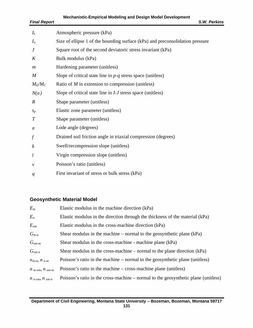
Mechanistic-Empirical Modeling and Design Model Development Final Report S.W. Perkins
Department of Civil Engineering, Montana State University – Bozeman, Bozeman, Montana 59717 131
IL Atmospheric pressure (kPa)
Io Size of ellipse 1 of the bounding surface (kPa) and preconsolidation pressure
J Square root of the second deviatoric stress invariant (kPa)
K Bulk modulus (kPa)
m Hardening parameter (unitless)
M Slope of critical state line in p-q stress space (unitless)
ME/MC Ratio of M in extension to compression (unitless)
N(α) Slope of critical state line in I-J stress space (unitless)
R Shape parameter (unitless)
sp Elastic zone parameter (unitless)
T Shape parameter (unitless)
α Lode angle (degrees)
φ Drained soil friction angle in triaxial compression (degrees)
κ Swell/recompression slope (unitless)
λ Virgin compression slope (unitless)
ν Poisson’s ratio (unitless)
θ First invariant of stress or bulk stress (kPa)
Geosynthetic Material Model
Em Elastic modulus in the machine direction (kPa)
En Elastic modulus in the direction through the thickness of the material (kPa)
Exm Elastic modulus in the cross-machine direction (kPa)
Gm-n Shear modulus in the machine – normal to the geosynthetic plane (kPa)
Gxm-m Shear modulus in the cross-machine - machine plane (kPa)
Gxm-n Shear modulus in the cross-machine – normal to the plane direction (kPa)
νm-n, ν n-m Poisson’s ratio in the machine – normal to the geosynthetic plane (unitless)
ν m-xm, ν xm-m Poisson’s ratio in the machine – cross-machine plane (unitless)
ν n-xm, ν xm-n Poisson’s ratio in the cross-machine – normal to the geosynthetic plane (unitless)

Mechanistic-Empirical Modeling and Design Model Development Final Report S.W. Perkins
Department of Civil Engineering, Montana State University – Bozeman, Bozeman, Montana 59717 132
APPENDIX B: DESIGN GUIDE B.1.0 INTRODUCTION
This appendix has been prepared for the final report of a research project titled “Mechanistic-
Empirical Modeling and Design Model Development of Geosynthetic Reinforced Flexible
Pavements” and is intended to serve as a stand-alone document summarizing the design model
described in the main body of the report and how this model should be used within the context of
pavement design practice. The intended audience for this appendix is the interested user of the
design model who is concerned principally with use of the model in practice. As such,
information concerning the development of the design model is excluded. Given the relatively
large number of equations associated with the design model and the availability of a spreadsheet
program through this project that performs these computations, non-essential design equations
are not contained in this guide but can be found in the body of the main report. It is assumed that
the spreadsheet program will be used and hence the design model is described within the context
of the program. The spreadsheet program may be downloaded from the following URL:
http://www.mdt.state.mt.us/departments/researchmgmt/grfp/grfp.html; or obtained by contacting
the Montana Department of Transportation, Development and Technology Transfer Program at
the address listed in the Technical Report Standard Page of this report.
B.2.0 APPLICATION BACKGROUND
The design guide presented in this appendix addresses the use of geosynthetics for reinforcement
in flexible pavement systems when placed at the bottom of the base or subbase aggregate layer.
Geosynthetic reinforcement within this context is intended to provide structural support of traffic
loads over the life of the pavement and principally addresses the pavement distress feature of
rutting due to the accumulation of permanent strain in the unbound aggregate and subgrade
layers. The geosynthetic is expected to provide one or a combination of the following two
primary benefits: 1) improved or extended service life of the pavement; 2) a reduction in base or
subbase aggregate thickness for equal service life. The types of geosynthetics that may be used
for this application include geotextiles, geogrids or geogrid/geotextile composites. The use of
geotextiles for separation and stabilization applications is addressed in AASHTO Specification
M-288 (AASHTO, 1997a).
Mechanistic-Empirical Modeling and Design Model Development Final Report S.W. Perkins
Department of Civil Engineering, Montana State University – Bozeman, Bozeman, Montana 59717 133
B.3.0 DESIGN MODEL BACKGROUND
The research project from which this appendix was developed provides a design model for the
application described in Section B.2.0. The design model was developed to describe
reinforcement benefit in terms of generic material and pavement layer parameters, thereby
allowing for the consideration of geosynthetic reinforcement for a range of pavement design
conditions and geosynthetic products.
The design model was developed within the context of a mechanistic-empirical analysis
framework. A finite element response model, including specific elements and material properties
for the geosynthetic reinforcement, was developed to provide key stress and strain response
measures that relate to the pavement distress feature of permanent surface deformation due to the
development of permanent strain in the unbound aggregate and subgrade layers. Empirical
distress models were either adopted and modified, or developed to relate the response measures
from the mechanistic finite element model to pavement performance defined in terms of
permanent surface deformation.
The finite element response model was used within the context of a parametric study to
analyze and provide response measures for over 465 pavement design configurations. The
empirical distress models used in the study were calibrated by the comparison of response
measures from certain finite element model cases to stress and strain measures from large-scale
tests sections reported by Perkins (1999a). The design model itself was further calibrated by
comparison of reinforcement benefit predicted from the model to that observed in these same
pavement test sections.
Regression equations were developed from the results of the parametric study to relate
reinforcement benefit to the range of input parameters used. These parameters included thickness
of the asphalt concrete and base course aggregate layers, strength/stiffness of the subgrade layer,
secant tensile modulus of the geosynthetic measured at 2 % axial strain in the strong direction of
the material, the ratio of secant tensile modulus between the weak and strong directions of the
material and two other elastic properties (Poisson’s ratio and shear modulus) that may be related
to geosynthetic type and structure. These regression equations form the basis of the design
model. The relatively large number of regression equations developed and the need for iterations
of several equations prompted the need to program them into a relatively simple spreadsheet
program available through this project.

Mechanistic-Empirical Modeling and Design Model Development Final Report S.W. Perkins
Department of Civil Engineering, Montana State University – Bozeman, Bozeman, Montana 59717 134
The design model, expressed in the form of the spreadsheet program, provides quantitative
descriptions of reinforcement benefit for the input parameters contained in the model. The
purpose of this design guide is to describe the operation of the design model including the input
required and the use of the benefit values for pavement design.
B.4.0 REINFORCEMENT BENEFIT DEFINITIONS
The design model predicts reinforcement benefit in terms of two basic parameters, namely
Traffic Benefit Ratio (TBR) and Base Course reduction Ratio (BCR). TBR describes the increase
in service life of an unreinforced pavement design when a particular geosynthetic reinforcement
is added. TBR is formally defined as the ratio of the number of traffic loads between an otherwise
identical reinforced and unreinforced pavement that are applied to reach a particular pavement
permanent surface deformation. BCR describes the reduction of base course aggregate allowed
for equivalent service life. BCR is formally defined as the percentage reduction of the base
course thickness of an unreinforced pavement such that equivalent life, defined in terms of traffic
loads, is obtained between the thinner reinforced pavement and the thicker unreinforced
pavement. As defined above, TBR corresponds to no reduction in base course aggregate
thickness and is more formally denoted as TBRBCR=0. BCR as defined above corresponds to no
increase in service life and is more formally denoted as BCRTBR=1. The design model allows for
the combined use of the two benefits described above by the determination of combined values
of TBR and BCR. When combined values are used, values will fall within the following ranges:
1 = TBR = TBRBCR=0; 0 = BCR = BCRTBR=1.
The use of a BCRTBR=1 will be most familiar conceptually because of its similarity to
methods employed for comparison of bound aggregate (i.e. cement treated base) to unbound
crushed base options. The use of bound aggregate requires that a more expensive material be
used with savings being realized by a reduction in the thickness of the layer for an equivalent
service life. This option will also require the least amount of effort in terms of a cost savings
analysis. It should be recognized, however, that the use of a TBR value, either as TBRBCR=0 or
combined with a BCR, will most likely yield the greatest economic benefits when life-cycle costs
are considered over the increased service life of the reinforced pavement. Transportation
agencies are encouraged to consider options involving the use of TBR to examine cost savings

Mechanistic-Empirical Modeling and Design Model Development Final Report S.W. Perkins
Department of Civil Engineering, Montana State University – Bozeman, Bozeman, Montana 59717 135
for typical projects. Examples are provided at the end of this guide that illustrate these
considerations.
The design model has been formulated to determine separate values of TBR and BCR for
reinforcement effects in the subgrade, base aggregate layer and for the total system. The report
for this project describes the conservatism and apparent safety associated with the steps taken to
develop the design model and concludes that reinforcement effects for the total system be used.
It is recommended, therefore, that the Total values column for TBR and/or BCR values in the
design spreadsheet program be used. Values for each reinforcement effect are provided,
however, such that designers may choose values at their discretion. All examples contained in
this guide use benefit values for the total system.
B.5.0 DESIGN MODEL
B.5.1 Design Model Input
The design model spreadsheet program requires specification of 20 input parameters. Figure
B.5.1 provides a diagram of the selection boxes for the input parameters with typical values
provided for one of the cases examined in the project. Comment boxes in the active program
provide information on each input item.
Table B.5.1 provides a listing of the 14 input parameters contained in the input selection
boxes for the Pavement Section Parameters and Geosynthetic Properties boxes shown in Figure
B.5.1. The parameters a1, a2 and a3 are dimensionless structural layer coefficients for the asphalt
concrete, base aggregate and subbase layers, respectively as defined for use in the AASHTO
1993 pavement design guide. While this design guide is general in the sense that the
unreinforced pavement can be designed according to any technique, as described later in this
appendix, input parameters for layer coefficients must be specified within the context of the
AASHTO 1993 guide. The 1993 guide contains equations and charts for relating dimensionless
layer coefficients to other commonly used parameters describing the mechanical properties of
these pavement layers and should be used to determine appropriate values of layer coefficients
for the design in question. A recently completed survey of US State transportation agencies
indicated that 70 % of the 34 responding agencies used the AASHTO 1993 method for pavement
design (Christopher et al., 2001).

Mechanistic-Empirical Modeling and Design Model Development Final Report S.W. Perkins
Department of Civil Engineering, Montana State University – Bozeman, Bozeman, Montana 59717 136
Figure B.5.1 Design model software program input selection boxes.

Mechanistic-Empirical Modeling and Design Model Development Final Report S.W. Perkins
Department of Civil Engineering, Montana State University – Bozeman, Bozeman, Montana 59717 137
1500SM
CBR =
Table B.5.1 Design model input parameters. a1 Asphalt concrete structural layer coefficient (unitless) a2 Base aggregate structural layer coefficient (unitless) a3 Subbase aggregate structural layer coefficient (unitless) CBR Subgrade California Bearing Ratio (%) D1 Asphalt concrete thickness (mm) D2 Base aggregate thickness (mm) D3 Subbase aggregate thickness (mm) GMR Ratio of minimum to maximum 2 % secant modulus of the geosynthetic (unitless) GSM-2% Secant tensile modulus from ASTM 4595 measured at 2 % axial strain (kN/m) m2 Base layer drainage coefficient (unitless) m3 Subbase layer drainage coefficient (unitless) RGI Reduction factor for interface shear (unitless) RGν Reduction for geosynthetic Poisson’s ratio (unitless) RGG Reduction for geosynthetic shear modulus (unitless)
The strength or stiffness of the subgrade material is specified by the design value for its
California Bearing Ratio (CBR). If the subgrade has been characterized in terms of a design
value for resilient modulus (MS), then subgrade CBR should be estimated from Equation B.5.1,
where resilient modulus in this equation should have units of psi. The survey contained in
Christopher et al. (2001) indicated that 41 % of responding agencies use CBR to characterize the
subgrade while 47 % use resilient modulus. Values of either CBR or MS should be the values
used for development of the unreinforced pavement design.
(B.5.1)
The parameters D1, D2 and D3 describe the layer thickness of the asphalt concrete, base
aggregate and subbase layers, respectively, for the unreinforced pavement design, where these
parameters should be specified in units of millimeters. The program internally converts the
calculated structural number in units of millimeters to units of inches for use in the AASHTO
design equation. The parameters m2 and m3 are the drainage coefficients for the base and subbase
layers, where these values must also be determined within the guidelines of the AASHTO 1993
method.
The parameters introduced above correspond to conventional pavement design parameters
used within the context of the AASHTO 1993 method. The remainder of this section describes
parameters pertinent to the geosynthetic reinforcement. As an aid for understanding these

Mechanistic-Empirical Modeling and Design Model Development Final Report S.W. Perkins
Department of Civil Engineering, Montana State University – Bozeman, Bozeman, Montana 59717 138
parameters, Table B.5.2 provides a listing of the geosynthetic products used in the study that
served as the basis for this design model. Table B.5.2 lists material characteristics for these
products as provided by the manufacturer. Table B.5.3 provides a summary of the geosynthetic
input parameters for the design model as they were used in the study for these materials. It
should be noted that only the “wide-width tensile strength at 2 % axial strain” data in Table B.5.2
is used for the determination of design model input parameters.
Table B.5.2 Material properties of geosynthetics used for design model development. Geogrid A: Geogrid B: Geotextile: Material Polypropylene Polypropylene Polypropylene Structure Punched
Drawn, Biaxial Punched
Drawn, Biaxial Woven
Mass/Unit Area (g/m2) 215 309 250
Aperature Size (mm) Machine Direction Cross-Machine Direction
25 33
25 33
None
Wide-Width Tensile Strength at 2 % Strain (kN/m) Machine Direction Cross-Machine Direction
5.06 8.5
7.32 11.9
4.25 13.6
Wide-Width Tensile Strength at 5 % Strain (kN/m) Machine Direction Cross-Machine Direction
9.71 16.5
13.4 22.9
11.9 26.4
Ultimate Wide-Width Tensile Strength (kN/m) Machine Direction Cross-Machine Direction
13.8 21.2
21.1 31.3
40.2 42.9
Table B.5.3 Design model parameters for geosynthetics. Geogrid A: Geogrid B: Geotextile: GSM-2% (kN/m) 425 595 680 GMR (unitless) 0.595 0.615 0.313 RGν (unitless) unchecked unchecked checked
RGG (unitless) unchecked unchecked checked RGI (unitless) 1.0 1.0 0.765
The parameters GSM-2% and GMR describe secant tensile modulus data for the two principal
directions of the geosynthetic. The parameter GSM-2% is the greatest value of secant tensile

Mechanistic-Empirical Modeling and Design Model Development Final Report S.W. Perkins
Department of Civil Engineering, Montana State University – Bozeman, Bozeman, Montana 59717 139
modulus for the two principal directions of the geosynthetic, where all modulus values have been
measured at an axial strain of 2 %. For example, GSM-2% for Geogrid A equals 8.5/0.02 = 425.
ASTM 4595 (ASTM, 2001a) should be followed to determine these values in each principal
direction of the geosynthetic. Values of modulus in units of kN/m should be used. The parameter
GMR is the ratio of the minimum to maximum 2 % secant tensile modulus for the two principal
directions of the geosynthetic. This parameter should be expressed in decimal form and should
be = 1. For Geogrid A, GMR = 5.06/8.5 = 0.595.
The parameters RGν and RGG are reduction factors for two other geosynthetic material
properties (in-plane Poisson’s ratio and shear modulus), which relate to the type and structure of
the geosynthetic. Each reduction factor corresponds to a check box in the spreadsheet program.
When unchecked, each factor has a value of 1.00 and corresponds to a good geosynthetic type
and structure for this application. When checked, reduction factors, as summarized in Table 7.6.1
of the main report, are applied to base, subgrade and total system reinforcement effects and
correspond to a less favorable geosynthetic type and structure for this application. Calibration of
the design model from large-scale test sections resulted in reduction factors of 1.00 (i.e.
unchecked boxes) for two rigid, extruded geogrid products and checked boxes for a woven, slit-
film geotextile. Suitable tests for the definition of these parameters have not been developed. In
the absence of a suitable test method and additional results from test sections using a broader
range of geosynthetic products, the values used above along with general geosynthetic
application guidelines provided in Berg et al. (2000) and summarized in Table 2.1.2 should serve
as the basis for selection of these parameters.
The parameter RGI defines a reduction factor for shear interaction characteristics between
the unbound aggregate and the geosynthetic layers and should have a value = 1. Calibration of
the design model from large-scale test sections resulted in a reduction factor of 1.00 for Geogrids
A and B and 0.765 for the Geotextile. Like the situation for definition of parameters RGν and
RGG, suitable tests for the definition of RGI have not been developed. The values provided above
should serve as a guide until additional information becomes available.
Figure B.5.1 contains six other input parameters contained in the Desired Reinforcement
Benefit selection boxes. Values of Desired TBR or BCR can be listed for reinforcement effects on
the subgrade, base or total system. These input boxes are provided for computing combined
values of TBR and BCR. When desired values are specified within the ranges 1 = Desired TBR =

Mechanistic-Empirical Modeling and Design Model Development Final Report S.W. Perkins
Department of Civil Engineering, Montana State University – Bozeman, Bozeman, Montana 59717 140
TBRBCR=0 and 0 = Desired BCR = BCRTBR=1, for any of the three categories of reinforcement
effect, remaining values of TBR or BCR are computed and listed in the output section. Values in
the Total column are recommended for use.
B.5.2 Design Model Output
Figure B.5.2 shows the output boxes for the spreadsheet program for the input parameters
contained in Figure B.5.1. Table B.5.4 provides a list of the parameters contained in the output
boxes.
Figure B.5.2 Design model software program output boxes.
Table B.5.4 Design model output parameters. BCRTBR=1 Base course reduction ratio (%) when TBR is 1 Desired BCR Input value for desired BCR (%) Remaining BCR Computed value of remaining BCR (%) for desired TBR specified as input MR-R/U Ratio of reinforced to unreinforced base aggregate resilient moduli TBRBCR=0 Traffic benefit ratio (unitless) when BCR is 0 Desired TBR Input value for desired TBR (unitless) Remaining TBR Computed value of remaining TBR for desired BCR specified as input
Values of TBRBCR=0 and BCRTBR=1 are provided for each of the three reinforcement effects
of base, subgrade and total system, and where recommended values for the total system have
been highlighted in yellow in the active spreadsheet. For the input parameters listed in Figure
B.5.1, values of TBRBCR=0 and BCRTBR=1 of 4.34 and 31.0 % are obtained. Values of Desired TBR
and Desired BCR in the output boxes are repeated from the input values provided. Values of

Mechanistic-Empirical Modeling and Design Model Development Final Report S.W. Perkins
Department of Civil Engineering, Montana State University – Bozeman, Bozeman, Montana 59717 141
Remaining TBR and Remaining BCR are computed based on the desired values specified and the
computed values for TBRBCR=0 and BCRTBR=1. As seen from the example provided, when values
of Desired TBR and Desired BCR of 1 and 0, respectively, are specified, then values of
Remaining TBR = TBRBCR=0 and Remaining BCR = BCRTBR=1. For the case of reinforcement
benefits for the total system, a Desired TBR = 2.0 results in a Remaining BCR = 17.1 %. A
Desired BCR = 25.0 % results in a Remaining TBR = 1.36.
Use of BCRTBR=1 typically requires only a consideration of construction costs when
performing a cost analysis of various pavement design options. Use of this parameter is
conceptually similar to consideration of stabilized base options, such as cement-treated base,
where a more expensive material with a reduced thickness is considered for construction. Since
an extension of service life is not involved in the use of BCRTBR=1, a life-cycle cost analysis is
generally not required. Use of TBRBCR=0 or combined values of TBR and BCR require that a life-
cycle cost analysis be performed to assess economic benefits. In general, it is anticipated that
options involving the use of TBR will yield the greatest economic benefits when life-cycle costs
are considered over the increased service life of the reinforced pavement. Transportation
agencies are encouraged to consider options involving the use of TBR to examine cost savings
for typical projects. Examples are provided at the end of this guide that illustrate these
considerations.
The last output parameter listed is the computed ratio of effective resilient modulus of the
reinforced and unreinforced base for reinforcement effects in the subgrade, base and total
system. These ratios are provided to allow a check on asphalt concrete fatigue cracking criteria
and should be used only for this purpose. It is recommended that the value listed for
reinforcement effects in the base layer be used, where this box has been highlighted in yellow in
the active spreadsheet. The design value for resilient modulus of the unreinforced base aggregate
layer should be multiplied by this ratio to obtain a design value for resilient modulus of the base
layer for the reinforced pavement. This value can then be used in a mechanistic analysis (layered
elastic or finite element) when checking the design for asphalt fatigue cracking. The user of this
factor should be reminded that the only pavement distress feature observed in the support testing
for this model was permanent surface deformation, meaning that this value is derived indirectly
from test results reflecting permanent deformation in the base aggregate and subgrade layers.
Consequently, this factor should be used with discretion and judgment.

Mechanistic-Empirical Modeling and Design Model Development Final Report S.W. Perkins
Department of Civil Engineering, Montana State University – Bozeman, Bozeman, Montana 59717 142
B.5.3 Design Model Input Limitations
The design model has been developed for a certain range of input parameters. Recommended
limits on critical parameters are given below:
1. 50 mm = D1 = 150 mm
2. 150 mm = D2 = 600 mm
3. 0.5 = Subgrade CBR = 15 or 5.2 MPa = MS = 155 MPa
4. 33 kN/m = GSM-2% = 2000 kN/m
5. BCR > 0 be used only for subgrades with a CBR = 1.0 (or MS = 10.3 MPa).
B.6.0 DESIGN STEPS
The design steps described below are an extension of those provided as the recommended
standard of practice in Berg et al. (2000) and AASHTO (2001). Additional details may be
obtained by referring to Berg et al. (2000).
Step 1. Initial assessment of applicability of the technology.
Step 2. Design of the unreinforced pavement.
Step 3. Definition of the qualitative benefits of reinforcement for the project.
Step 4. Definition of the quantitative benefits of reinforcement (TBR and/or BCR).
Step 5. Design of the reinforced pavement using the benefits defined in Step 4.
Step 6. Analysis of life-cycle costs.
Step 7. Development of a project specification.
Step 8. Development of construction drawings and bid documents.
Step 9. Construction of the roadway.
Step 1 involves consideration of project conditions for the design to determine whether
geosynthetic reinforcement is applicable and remains unchanged from that contained in Berg et
al. (2000). Step 2 involves designing the thickness of an unreinforced pavement section based on
representative material parameters. Step 2 may be accomplished by any recognized pavement
design procedure, provided that the pavement layer material properties can be related to the layer
coefficients and drainage coefficients required in the design model. Step 3 should emphasize the
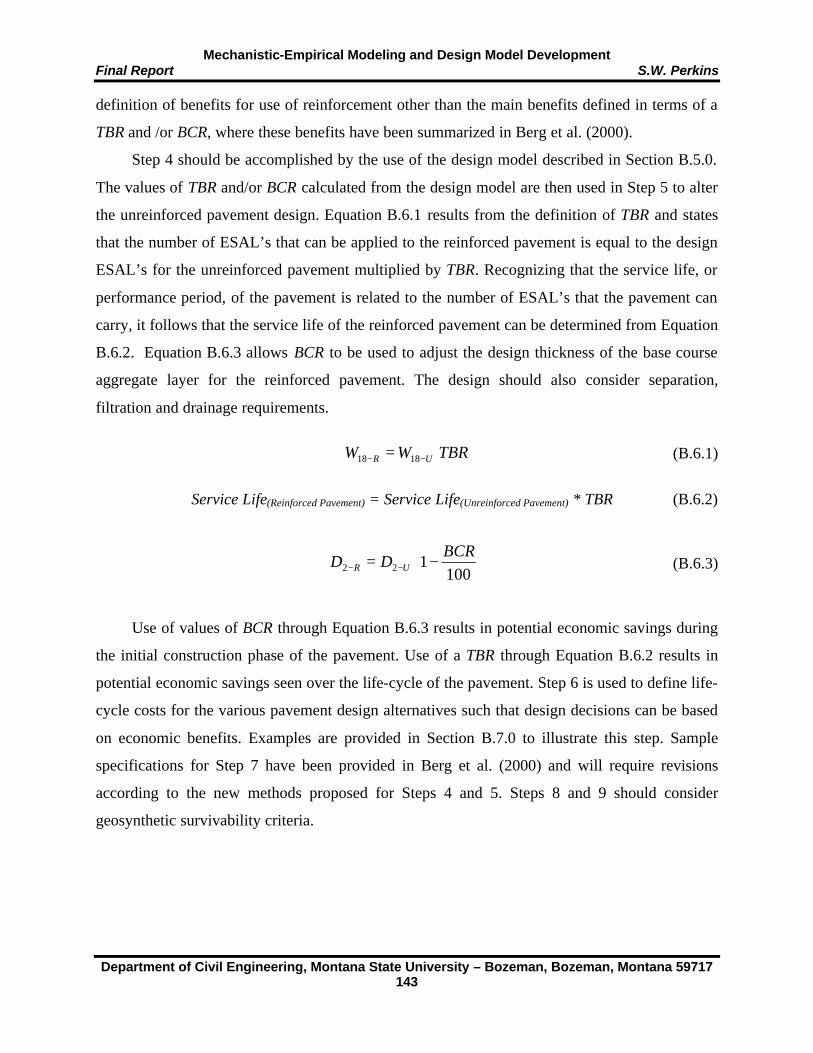
Mechanistic-Empirical Modeling and Design Model Development Final Report S.W. Perkins
Department of Civil Engineering, Montana State University – Bozeman, Bozeman, Montana 59717 143
−= −− 100122
BCRDD UR
TBRWW UR −− = 1818
definition of benefits for use of reinforcement other than the main benefits defined in terms of a
TBR and /or BCR, where these benefits have been summarized in Berg et al. (2000).
Step 4 should be accomplished by the use of the design model described in Section B.5.0.
The values of TBR and/or BCR calculated from the design model are then used in Step 5 to alter
the unreinforced pavement design. Equation B.6.1 results from the definition of TBR and states
that the number of ESAL’s that can be applied to the reinforced pavement is equal to the design
ESAL’s for the unreinforced pavement multiplied by TBR. Recognizing that the service life, or
performance period, of the pavement is related to the number of ESAL’s that the pavement can
carry, it follows that the service life of the reinforced pavement can be determined from Equation
B.6.2. Equation B.6.3 allows BCR to be used to adjust the design thickness of the base course
aggregate layer for the reinforced pavement. The design should also consider separation,
filtration and drainage requirements.
(B.6.1)
Service Life(Reinforced Pavement) = Service Life(Unreinforced Pavement) * TBR (B.6.2)
(B.6.3)
Use of values of BCR through Equation B.6.3 results in potential economic savings during
the initial construction phase of the pavement. Use of a TBR through Equation B.6.2 results in
potential economic savings seen over the life-cycle of the pavement. Step 6 is used to define life-
cycle costs for the various pavement design alternatives such that design decisions can be based
on economic benefits. Examples are provided in Section B.7.0 to illustrate this step. Sample
specifications for Step 7 have been provided in Berg et al. (2000) and will require revisions
according to the new methods proposed for Steps 4 and 5. Steps 8 and 9 should consider
geosynthetic survivability criteria.

Mechanistic-Empirical Modeling and Design Model Development Final Report S.W. Perkins
Department of Civil Engineering, Montana State University – Bozeman, Bozeman, Montana 59717 144
B.7.0 DESIGN EXAMPLES
Two basic examples are provided to illustrate use of the design model for pavement design. The
first example uses life-cycle cost information contained in Chapter 6 of Berg et al. (2000). The
rehabilitation steps contained in this example are kept relatively simple to avoid confusion. The
second example uses information from a project design recently prepared for the Montana
Department of Transportation. All examples were analyzed using the computer program
DARWin (AASHTO, 1997b), which is based on the AASHTO 1993 pavement design guide
(AASHTO, 1993). Copies of DARWin output are provided for each example in Appendix C as a
separate volume to this report (Perkins 2001b). Each example incorporates assumptions for
rehabilitation and maintenance steps and costs. These design assumptions will differ between
agencies, geographic locations, projects, designers and clients. The purpose of these examples is
to illustrate how reinforcement concepts and results from the design model can be incorporated
into life-cycle cost analyses. The focus should not be on the validity of the design assumptions
made for a particular agency or project, as these may vary as described above.
B.7.1 Illustrative Example
The first example is designed primarily to illustrate the operation of the design model and the
incorporation of the results into a life-cycle cost analysis. Table B.7.1 provides the input used for
the DARWin Flexible Structural Design module. These input design parameters result in a
structural number of 80 mm (3.1 in).
Table B.7.1 Flexible structural design module input for example 1. ESAL’s (W18) 35,000 Initial Serviceability 4.2 Terminal Serviceability 2.5 Reliability Level (%) 90 Overall Standard Deviation 0.44 Roadbed Soil Resilient Modulus (kPa) 15,500 Design Structural Number (mm) 80 Asphalt Concrete Layer One-Directional Lane Width (m) 4 Base Course Aggregate Layer One-Directional Lane Width (m) 5
Table B.7.2 lists the thickness design for the unreinforced pavement (Option 1) satisfying
the design structural number of 80 mm. Several design options with three different geosynthetics

Mechanistic-Empirical Modeling and Design Model Development Final Report S.W. Perkins
Department of Civil Engineering, Montana State University – Bozeman, Bozeman, Montana 59717 145
were considered. Geogrid A and B, and the Geotextile listed previously in Table B.5.2 were
used. Figures B.7.1 – B.7.3 provide a copy of the input and output from the design model for
each of the three geosynthetics. Each of the geosynthetic input parameter sets corresponds to
those values used for calibration of the model and are representative of these material types. For
cases where a TBRBCR=0 greater than 2 was obtained, options involving the combined use of BCR
and TBR were examined. Tables B.7.2 and B.7.3 provide a listing of the thickness design and
benefit values used for the design options examined. It should be noted that for the Geotextile, a
value of TBRBCR=0 = 2 was rounded up from the value of 1.97 computed from the design model.
The reduced base course aggregate thickness listed in Table B.7.2 for options using a BCR is
computed using Equation B.6.3.
Table B.7.2 Thickness designs for design options for example 1. Asphalt Concrete Base Course Aggregate Design
Option Structural Section Type
Thickness (mm)
Structural Coefficient
Thickness (mm)
Structural Coefficient
Option 1 Unreinforced 85 0.4 325 0.14 Option 2 Geogrid A 85 0.4 325 0.14 Option 3 Geogrid A 85 0.4 275 0.14 Option 4 Geogrid A 85 0.4 228 0.14 Option 5 Geogrid B 85 0.4 306 0.14 Option 6 Geogrid B 85 0.4 259 0.14 Option 7 Geogrid B 85 0.4 215 0.14 Option 8 Geotextile 85 0.4 325 0.14 Option 9 Geotextile 85 0.4 271 0.14
Table B.7.3 TBR and BCR values for design options for example 1. Design Option Structural Section Type TBRT BCRT
Option 1 Unreinforced NA NA Option 2 Geogrid A 4 0 Option 3 Geogrid A 2 15.5 Option 4 Geogrid A 1 29.7 Option 5 Geogrid B 4 5.7 Option 6 Geogrid B 2 20.3 Option 7 Geogrid B 1 33.7 Option 8 Geotextile 2 0 Option 9 Geotextile 1 16.6
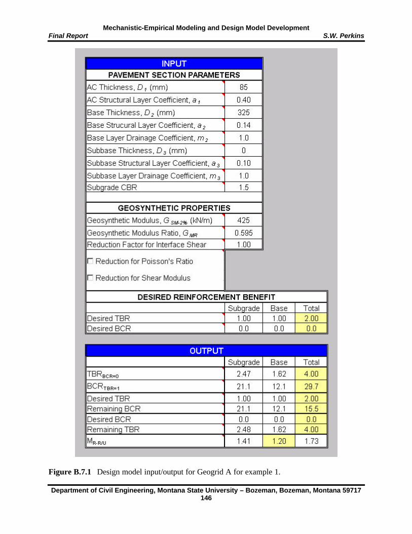
Mechanistic-Empirical Modeling and Design Model Development Final Report S.W. Perkins
Department of Civil Engineering, Montana State University – Bozeman, Bozeman, Montana 59717 146
Figure B.7.1 Design model input/output for Geogrid A for example 1.
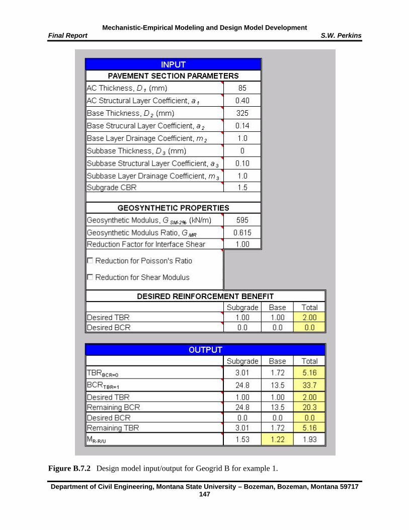
Mechanistic-Empirical Modeling and Design Model Development Final Report S.W. Perkins
Department of Civil Engineering, Montana State University – Bozeman, Bozeman, Montana 59717 147
Figure B.7.2 Design model input/output for Geogrid B for example 1.

Mechanistic-Empirical Modeling and Design Model Development Final Report S.W. Perkins
Department of Civil Engineering, Montana State University – Bozeman, Bozeman, Montana 59717 148
Figure B.7.3 Design model input/output for Geotexile for example 1.

Mechanistic-Empirical Modeling and Design Model Development Final Report S.W. Perkins
Department of Civil Engineering, Montana State University – Bozeman, Bozeman, Montana 59717 149
A life-cycle cost analysis was performed for each design option. Table B.7.4 lists the
assumed construction and rehabilitation dates and performance periods for each design option.
This relatively simple example assumes that the performance period of the new pavement for the
unreinforced option is 10 years. The example assumes that the pavement will be milled and
overlaid every 10 years. An overlay thickness of 50 mm is assumed. These assumptions are
purposefully simplistic in order to illustrate the incorporation of reinforcement concepts and
results from the design model into a life-cycle cost analysis.
Table B.7.4 Construction and rehabilitation dates and performance periods for example 1. Date of Step Taken and Performance Period (years) Step
Options 1, 4 & 7 Options 3, 6 & 8 Options 2 & 5 New Construction 2000 / 10 2000 / 20 2000 / 40 Asphalt Concrete Milling and Overlay 2010 / 10 2020 / 20 Asphalt Concrete Milling and Overlay 2020 / 10 Asphalt Concrete Milling and Overlay 2030 / 10
Use of a TBR of 2 for options 3, 6 and 8 allows the performance period for the new
construction to be extended from 10 years to 20 years. In addition, it is assumed that the milling
and overlay rehabilitation at year 2020 has a performance period of 20 rather than 10 years. Use
of a TBR of 4 for options 2 and 5 allows the performance period for the new construction of 10
years to be extended to 40 years such that no rehabilitations are required within the analysis
period of 40 years. This approach assumes that rutting in the pavement is due primarily to
permanent deformation in the base and subgrade layers, which is influenced by reinforcement.
This is generally believed to be true of relatively thin pavement sections. For thick pavement
layers, rutting and subsequent milling and overlays will most likely be controlled more by flow
within the AC layer, which is not effected by reinforcement. The example given in Section B.7.2
assumes that milling and overlays are required equally for all options, but that reconstruction
costs are impacted by the extension of service life.
Other design inputs and pay item costs for the analysis are listed in Tables B.7.5 and B.7.6.
The maintenance cost listed in Table B.7.6 is assumed to begin 5 years after each performance
period, meaning that 20 years of maintenance is included for options 1, 4 and 7, 30 years is
included for options 3, 6 and 8 and 35 years is included for options 2 and 5. The costs used for
the three geosynthetics are based on the author’s experience and best judgment. These costs, and
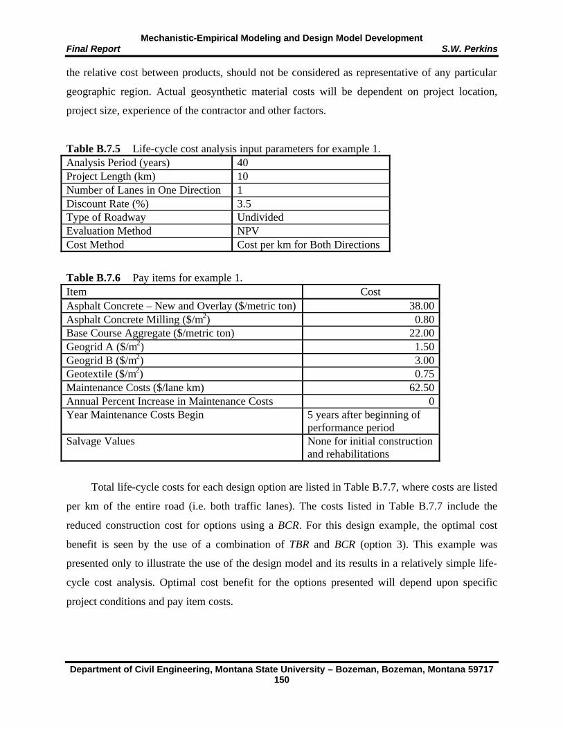
Mechanistic-Empirical Modeling and Design Model Development Final Report S.W. Perkins
Department of Civil Engineering, Montana State University – Bozeman, Bozeman, Montana 59717 150
the relative cost between products, should not be considered as representative of any particular
geographic region. Actual geosynthetic material costs will be dependent on project location,
project size, experience of the contractor and other factors.
Table B.7.5 Life-cycle cost analysis input parameters for example 1. Analysis Period (years) 40 Project Length (km) 10 Number of Lanes in One Direction 1 Discount Rate (%) 3.5 Type of Roadway Undivided Evaluation Method NPV Cost Method Cost per km for Both Directions
Table B.7.6 Pay items for example 1. Item Cost Asphalt Concrete – New and Overlay ($/metric ton) 38.00 Asphalt Concrete Milling ($/m2) 0.80 Base Course Aggregate ($/metric ton) 22.00 Geogrid A ($/m2) 1.50 Geogrid B ($/m2) 3.00 Geotextile ($/m2) 0.75 Maintenance Costs ($/lane km) 62.50 Annual Percent Increase in Maintenance Costs 0 Year Maintenance Costs Begin 5 years after beginning of
performance period Salvage Values None for initial construction
and rehabilitations
Total life-cycle costs for each design option are listed in Table B.7.7, where costs are listed
per km of the entire road (i.e. both traffic lanes). The costs listed in Table B.7.7 include the
reduced construction cost for options using a BCR. For this design example, the optimal cost
benefit is seen by the use of a combination of TBR and BCR (option 3). This example was
presented only to illustrate the use of the design model and its results in a relatively simple life-
cycle cost analysis. Optimal cost benefit for the options presented will depend upon specific
project conditions and pay item costs.

Mechanistic-Empirical Modeling and Design Model Development Final Report S.W. Perkins
Department of Civil Engineering, Montana State University – Bozeman, Bozeman, Montana 59717 151
Table B.7.7 Total life-cycle costs for design options for example 1. Design Option
Structural Section Type
Total Life Cycle Cost per km ($)
Percent Savings
Option 1 Unreinforced 269,210 NA Option 2 Geogrid A 221,641 17.7 Option 3 Geogrid A 219,159 18.6 Option 4 Geogrid A 240,484 10.7 Option 5 Geogrid B 228,076 15.3 Option 6 Geogrid B 226,947 15.7 Option 7 Geogrid B 249,624 7.3 Option 8 Geotextile 234,198 13.0 Option 9 Geotextile 252,368 6.3
B.7.2 Project Example
The second example uses design and analysis information from a project recently developed for
the Montana Department of Transportation (Allied Engineering, 2000). The example attempts to
use more comprehensive construction and life-cycle cost rehabilitation information. Assumptions
were necessary for rehabilitation and maintenance steps and costs. These assumptions will differ
from user to user. The purpose of this example is to illustrate the use of reinforcement benefit
within the context of a more complex project example. Agencies are encouraged to examine life-
cycle cost scenarios pertinent to conditions within their jurisdictions.
The project consists of the reconstruction of 17.5 km of US Highway 12 between the towns
of Melstone and Sumatra located approximately 130 km northeast of Billings, Montana. The age
of the roadway required complete removal and replacement of the existing pavement structure
and partial realignment. Input for the flexible structural design module is listed in Table B.7.8,
which assumes a 20-year design life. Four design options are considered. Option 1 uses an
unbound, unreinforced crushed base aggregate. Option 2 uses a cement treated base for the base
aggregate layer. Options 3 and 4 use Geogrid A for base reinforcement. Input to the spreadsheet
design model is shown in Figure B.7.4, where a TBRBCR=0 = 2.21 was obtained. Option 3 is
developed by specifying a desired TBR of 2, which provides a remaining BCR of 2.3 %. Option 4
uses a BCR of 18.5 % for a TBR = 1. Thickness designs and TBR/BCR values used for options 3
and 4 are listed in Tables B.7.9 and B.7.10.

Mechanistic-Empirical Modeling and Design Model Development Final Report S.W. Perkins
Department of Civil Engineering, Montana State University – Bozeman, Bozeman, Montana 59717 152
Figure B.7.4 Design model input/output for example 2.

Mechanistic-Empirical Modeling and Design Model Development Final Report S.W. Perkins
Department of Civil Engineering, Montana State University – Bozeman, Bozeman, Montana 59717 153
Table B.7.8 Flexible structural design module input for example 2. ESAL’s (W18) 165,549 Initial Serviceability 4.2 Terminal Serviceability 2.5 Reliability Level (%) 90 Overall Standard Deviation 0.35 Roadbed Soil Resilient Modulus (kPa) 31,000 Design Structural Number (mm) 76
Table B.7.9 Thickness designs for design options for example 2. Asphalt Concrete Base Course Aggregate Design
Option Structural Section Type
Thickness (mm)
Structural Coefficient
Thickness (mm)
Structural Coefficient
Drainage Coefficient
Option 1 Unreinforced 90 0.33 486 0.095 1.0 Option 2 CTB 90 0.33 257 0.18 1.0 Option 3 Geogrid A 90 0.33 475 0.095 1.0 Option 4 Geogrid A 90 0.33 398 0.095 1.0
Table B.7.10 TBR and BCR values for design options for example 2. Design Option Structural Section Type TBRT BCRT
Option 1 Unreinforced NA NA Option 2 Cement Treated Base NA NA Option 3 Geogrid A 2 1.5 Option 4 Geogrid A 0 18.5
The life-cycle cost analysis used the construction and rehabilitation steps, dates and
performance periods listed in Table B.7.11. In this example, the newly constructed road was chip
sealed immediately after construction. Crack sealing and chip sealing is a rehabilitation step
required every 5 years and is assumed not to be effected by TBR. A milling thickness of 75 mm
was used for determining the overlay thickness. An overlay design within DARWin using the
remaining life method resulted in a total overlay thickness of 79 mm. Milling and overlays were
required every 10 years for all options and were assumed to be necessary because of asphalt
concrete rutting due to flow within the AC layer, which is not effected by reinforcement. Some
of this rutting may in fact be due to permanent deformation in the base and subgrade layers, in
which case reinforcement would limit this for option 3.
A design life of 20 years required that the asphalt concrete layer be removed and
reconstructed at year 2020 for options 1, 2 and 4. A TBR of 2 eliminated the need for this
rehabilitation step for option 3. This constitutes the major difference between option 3 and the

Mechanistic-Empirical Modeling and Design Model Development Final Report S.W. Perkins
Department of Civil Engineering, Montana State University – Bozeman, Bozeman, Montana 59717 154
others. The asphalt concrete was removed by complete milling of the layer and incorporation of
the material back into the base aggregate layer. Traffic control was assumed to be required for
this rehabilitation step.
Table B.7.11 Construction and rehabilitation dates and performance periods for example 2. Step Taken Date of Step & Performance
Period (years) Options 1, 2 & 4 Option 3 2000 / 5 New Construction and Chip
Seal New Construction and Chip Seal
2005 / 5 Crack Sealing and Chip Seal Crack Sealing and Chip Seal 2010 / 5 Asphalt Concrete Milling,
Overlay and Chip Seal Asphalt Concrete Milling, Overlay and Chip Seal
2015 / 5 Crack Sealing and Chip Seal Crack Sealing and Chip Seal 2020 /5 Remove/Reconstruct Asphalt
Concrete and Chip Seal Asphalt Concrete Milling, Overlay and Chip Seal
2025 / 5 Crack Sealing and Chip Seal Crack Sealing and Chip Seal 2030 / 5 Asphalt Concrete Milling,
Overlay and Chip Seal Asphalt Concrete Milling, Overlay and Chip Seal
2035 / 5 Crack Sealing and Chip Seal Crack Sealing and Chip Seal
Reconstruction of the pavement section for options 1, 2 and 4 at year 20 was different
between the options. Since option 1 did not contain any type of geosynthetic, a certain amount of
base course contamination was assumed to occur over the first 20-year design life. At year 20, it
was assumed that the base aggregate had gone from a material in a damp to dry state having a
resilient modulus of 139 MPa and a layer coefficient of 0.095 to a material in a moist to damp
state having a resilient modulus of 100 MPa and a layer coefficient of 0.06. In addition, assumed
contamination of the base required that the drainage coefficient be reduced from 1.0 for the
original construction to 0.6 for the reconstruction. Based on these values, a new AC thickness
was computed to carry the 20-year design ESAL’s for the second 20-year period. Table B.7.12
provides a summary of these details for each option.

Mechanistic-Empirical Modeling and Design Model Development Final Report S.W. Perkins
Department of Civil Engineering, Montana State University – Bozeman, Bozeman, Montana 59717 155
Table B.7.12 Thickness designs for options 1, 2 and 4 for reconstruction at year 20. Asphalt Concrete Base Course Aggregate Design
Option Thickness (mm)
Structural Coefficient
Thickness (mm)
Structural Coefficient
Drainage Coefficient
Option 1 177 0.33 486 0.06 0.6 Option 2 145 0.33 257 0.11 1.0 Option 4 137 0.33 398 0.079 0.8
Cement treated bases are known to deteriorate and lose strength in the presence of
moisture. For option 2, it was assumed that the cement treated base lost approximately 50 % of
its assumed modulus when it was originally constructed. This results in the use of a layer
coefficient of 0.11 for the cement treated base for the reconstruction design. The drainage
coefficient was maintained at a value of 1.0.
Some level of contamination of the base aggregate layer was assumed for option 4 using a
geogrid reinforcement. The reduction in layer properties was assumed to be approximately half
of that used for option 1. The resilient modulus of the base aggregate was assumed to reduce
from the initial value of 139 MPa to 120 MPa, yielding a layer coefficient of 0.079. The drainage
coefficient was assumed to reduce from 1.0 to 0.8.
The lane and layer widths were established such that the minimum one-lane AC surface
deck width of 4.6 m was maintained throughout the 40-year analysis period. In addition, the
design side slope of 1V:11H was maintained for all layers.
Tables B.7.13 and B.7.14 give life-cycle cost analysis input parameters and pay item
information. The pay item information was derived from the project report (Allied Engineering,
2000) and average contractor bid summaries for the year 2000, as available from the Montana
DOT (MDT, 2001). Maintenance costs were not included as the pay items of crack and chip
sealing required every 5 years were considered as maintenance.
Total life-cycle cost figures for each design option are listed in Table B.7.15. For this
particular example, it is seen that option 3 is the least expensive, followed by options 2 and 4.
This example disregards several considerations that may be examined for other cases. Any
differences in subexcavation costs between the different options were ignored. Options 2, 3 and 4
all involve a total pavement layer thickness at year-40 which is less than that of option 1, with
option 2 yielding the smallest total thickness. Reduced subexcavation costs would be anticipated
for options 2, 3 and 4. General assumptions were made regarding the level of deterioration of
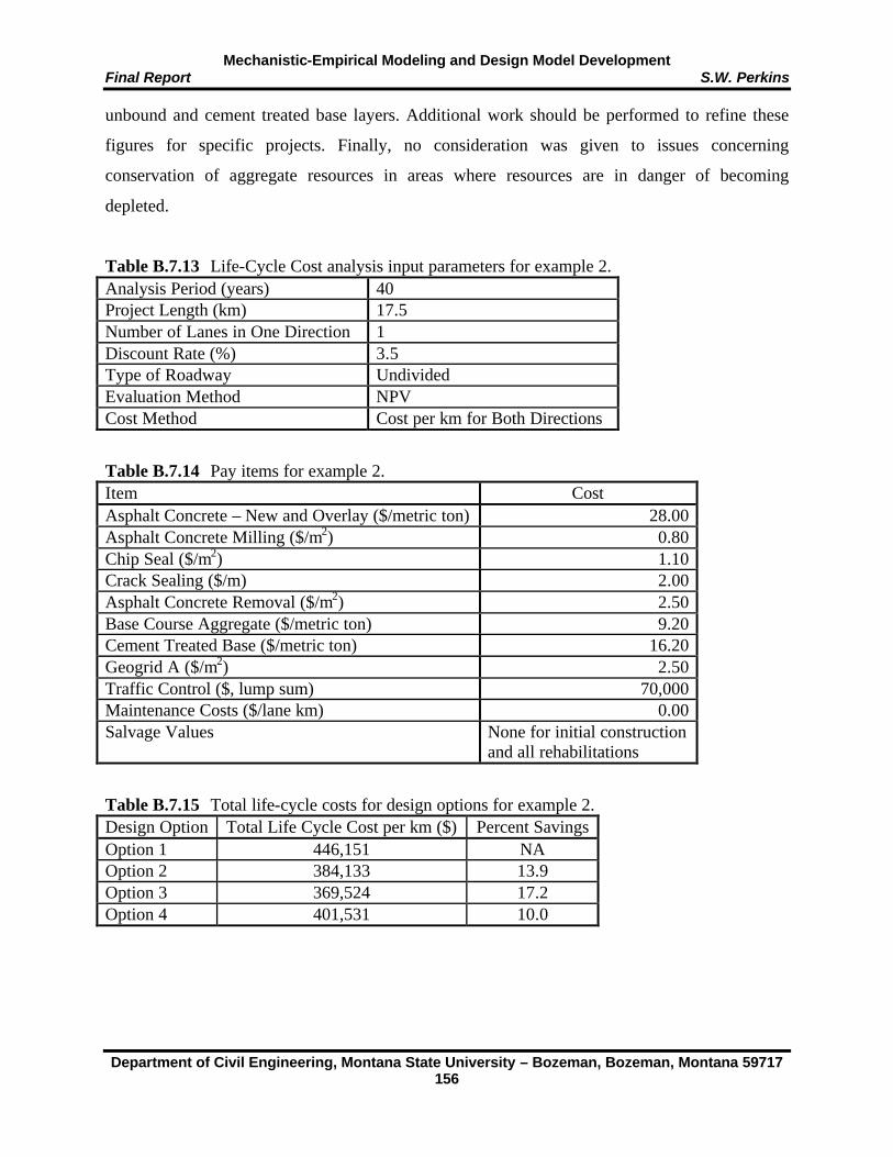
Mechanistic-Empirical Modeling and Design Model Development Final Report S.W. Perkins
Department of Civil Engineering, Montana State University – Bozeman, Bozeman, Montana 59717 156
unbound and cement treated base layers. Additional work should be performed to refine these
figures for specific projects. Finally, no consideration was given to issues concerning
conservation of aggregate resources in areas where resources are in danger of becoming
depleted.
Table B.7.13 Life-Cycle Cost analysis input parameters for example 2. Analysis Period (years) 40 Project Length (km) 17.5 Number of Lanes in One Direction 1 Discount Rate (%) 3.5 Type of Roadway Undivided Evaluation Method NPV Cost Method Cost per km for Both Directions
Table B.7.14 Pay items for example 2. Item Cost Asphalt Concrete – New and Overlay ($/metric ton) 28.00 Asphalt Concrete Milling ($/m2) 0.80 Chip Seal ($/m2) 1.10 Crack Sealing ($/m) 2.00 Asphalt Concrete Removal ($/m2) 2.50 Base Course Aggregate ($/metric ton) 9.20 Cement Treated Base ($/metric ton) 16.20 Geogrid A ($/m2) 2.50 Traffic Control ($, lump sum) 70,000 Maintenance Costs ($/lane km) 0.00 Salvage Values None for initial construction
and all rehabilitations
Table B.7.15 Total life-cycle costs for design options for example 2. Design Option Total Life Cycle Cost per km ($) Percent Savings Option 1 446,151 NA Option 2 384,133 13.9 Option 3 369,524 17.2 Option 4 401,531 10.0