research designs - gary king
TRANSCRIPT

Advanced Quantitative Research Methodology, LectureNotes: Research Designs for Causal Inference1
Gary King
GaryKing.org
April 14, 2013
1 c©Copyright 2013 Gary King, All Rights Reserved.Gary King () Research Designs April 14, 2013 1 / 23

Reference
Kosuke Imai, Gary King, and Elizabeth Stuart. Misunderstandingsamong Experimentalists and Observationalists: Balance Test Fallaciesin Causal Inference Journal of the Royal Statistical Society, Series AVol. 171, Part 2 (2008): Pp. 1-22http://gking.harvard.edu/files/abs/matchse-abs.shtml
Gary King (Harvard) Research Designs for Causal Inference April 14, 2013 2 / 23

Notation
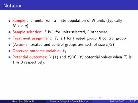
Sample of n units from a finite population of N units (typicallyN >> n)
Sample selection: Ii is 1 for units selected, 0 otherwise
Treatment assignment: Ti is 1 for treated group, 0 control group
(Assume: treated and control groups are each of size n/2)
Observed outcome variable: Yi
Potential outcomes: Yi (1) and Yi (0), Yi potential values when Ti is1 or 0 respectively.
Fundamental problem of causal inference. Only one potentialoutcome is ever observed:If Ti = 0, Yi (0) = Yi Yi (1) = ?If Ti = 1, Yi (0) = ? Yi (1) = Yi
(Ii ,Ti ,Yi ) are random; Yi (1) and Yi (0) are fixed.
Gary King (Harvard) Research Designs for Causal Inference April 14, 2013 3 / 23
Notation
Sample of n units from a finite population of N units (typicallyN >> n)
Sample selection: Ii is 1 for units selected, 0 otherwise
Treatment assignment: Ti is 1 for treated group, 0 control group
(Assume: treated and control groups are each of size n/2)
Observed outcome variable: Yi
Potential outcomes: Yi (1) and Yi (0), Yi potential values when Ti is1 or 0 respectively.
Fundamental problem of causal inference. Only one potentialoutcome is ever observed:If Ti = 0, Yi (0) = Yi Yi (1) = ?If Ti = 1, Yi (0) = ? Yi (1) = Yi
(Ii ,Ti ,Yi ) are random; Yi (1) and Yi (0) are fixed.
Gary King (Harvard) Research Designs for Causal Inference April 14, 2013 3 / 23
Quantities of Interest
Treatment Effect (for unit i):
TEi ≡ Yi (1)− Yi (0)
Population Average Treatment Effect:
PATE ≡ 1
N
N∑i=1
TEi
Sample Average Treatment Effect:
SATE ≡ 1
n
∑i∈{Ii=1}
TEi
Gary King (Harvard) Research Designs for Causal Inference April 14, 2013 4 / 23

Quantities of Interest
Treatment Effect (for unit i):
TEi ≡ Yi (1)− Yi (0)
Population Average Treatment Effect:
PATE ≡ 1
N
N∑i=1
TEi
Sample Average Treatment Effect:
SATE ≡ 1
n
∑i∈{Ii=1}
TEi
Gary King (Harvard) Research Designs for Causal Inference April 14, 2013 4 / 23

Quantities of Interest
Treatment Effect (for unit i):
TEi ≡ Yi (1)− Yi (0)
Population Average Treatment Effect:
PATE ≡ 1
N
N∑i=1
TEi
Sample Average Treatment Effect:
SATE ≡ 1
n
∑i∈{Ii=1}
TEi
Gary King (Harvard) Research Designs for Causal Inference April 14, 2013 4 / 23

Quantities of Interest
Treatment Effect (for unit i):
TEi ≡ Yi (1)− Yi (0)
Population Average Treatment Effect:
PATE ≡ 1
N
N∑i=1
TEi
Sample Average Treatment Effect:
SATE ≡ 1
n
∑i∈{Ii=1}
TEi
Gary King (Harvard) Research Designs for Causal Inference April 14, 2013 4 / 23

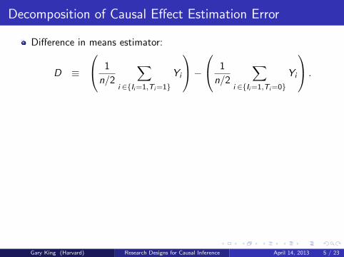
Decomposition of Causal Effect Estimation Error
Difference in means estimator:
D ≡
1
n/2
∑i ∈{Ii=1,Ti=1}
Yi
−
1
n/2
∑i ∈{Ii=1,Ti=0}
Yi
.
Estimation Error:
∆ ≡ PATE− D
Pretreatment confounders: X are observed and U are unobserved
Decomposition:
∆ = ∆S + ∆T
= (∆SX+ ∆SU
) + (∆TX+ ∆TU
)
Error due to ∆S (sample selection), ∆T (treatment imbalance), andeach due to observed (Xi ) and unobserved (Ui ) covariates
Gary King (Harvard) Research Designs for Causal Inference April 14, 2013 5 / 23

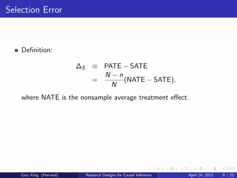
Selection Error
Definition:
∆S ≡ PATE− SATE
=N − n
N(NATE− SATE),
where NATE is the nonsample average treatment effect.
∆S vanishes if:
1 The sample is a census (Ii = 1 for all observations and n = N);2 SATE = NATE; or3 Switch quantity of interest from PATE to SATE (recommended!)
Gary King (Harvard) Research Designs for Causal Inference April 14, 2013 6 / 23

Selection Error
Definition:
∆S ≡ PATE− SATE
=N − n
N(NATE− SATE),
where NATE is the nonsample average treatment effect.
∆S vanishes if:1 The sample is a census (Ii = 1 for all observations and n = N);
2 SATE = NATE; or3 Switch quantity of interest from PATE to SATE (recommended!)
Gary King (Harvard) Research Designs for Causal Inference April 14, 2013 6 / 23

Selection Error
Definition:
∆S ≡ PATE− SATE
=N − n
N(NATE− SATE),
where NATE is the nonsample average treatment effect.
∆S vanishes if:1 The sample is a census (Ii = 1 for all observations and n = N);2 SATE = NATE; or
3 Switch quantity of interest from PATE to SATE (recommended!)
Gary King (Harvard) Research Designs for Causal Inference April 14, 2013 6 / 23

Selection Error
Definition:
∆S ≡ PATE− SATE
=N − n
N(NATE− SATE),
where NATE is the nonsample average treatment effect.
∆S vanishes if:1 The sample is a census (Ii = 1 for all observations and n = N);2 SATE = NATE; or3 Switch quantity of interest from PATE to SATE (recommended!)
Gary King (Harvard) Research Designs for Causal Inference April 14, 2013 6 / 23

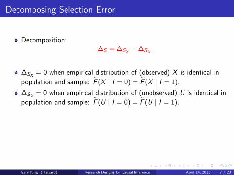
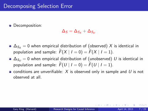
Decomposing Selection Error
Decomposition:∆S = ∆SX
+ ∆SU
∆SX= 0 when empirical distribution of (observed) X is identical in
population and sample: F̃ (X | I = 0) = F̃ (X | I = 1).
∆SU= 0 when empirical distribution of (unobserved) U is identical in
population and sample: F̃ (U | I = 0) = F̃ (U | I = 1).
conditions are unverifiable: X is observed only in sample and U is notobserved at all.
∆SXvanishes if weighting on X
∆SUcannot be corrected after the fact
Gary King (Harvard) Research Designs for Causal Inference April 14, 2013 7 / 23

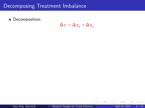
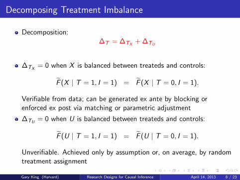
Decomposing Treatment Imbalance
Decomposition:∆T = ∆TX
+ ∆TU
∆TX= 0 when X is balanced between treateds and controls:
F̃ (X | T = 1, I = 1) = F̃ (X | T = 0, I = 1).
Verifiable from data; can be generated ex ante by blocking orenforced ex post via matching or parametric adjustment
∆TU= 0 when U is balanced between treateds and controls:
F̃ (U | T = 1, I = 1) = F̃ (U | T = 0, I = 1).
Unverifiable. Achieved only by assumption or, on average, by randomtreatment assignment
Gary King (Harvard) Research Designs for Causal Inference April 14, 2013 8 / 23

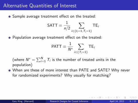
Alternative Quantities of Interest
Sample average treatment effect on the treated:
SATT ≡ 1
n/2
∑i∈{Ii=1,Ti=1}
TEi
Population average treatment effect on the treated:
PATT ≡ 1
N∗
∑i∈{Ti=1}
TEi
(where N∗ =∑N
i=1 Ti is the number of treated units in thepopulation)
When are these of more interest than PATE and SATE? Why neverfor randomized experiments? Why usually for matching?
Analogous estimation error decomposition: ∆′ = PATT− D, holds:
∆′ = (∆′SX
+ ∆′SU
) + (∆′TX
+ ∆′TU
)
Gary King (Harvard) Research Designs for Causal Inference April 14, 2013 9 / 23

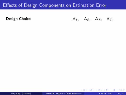
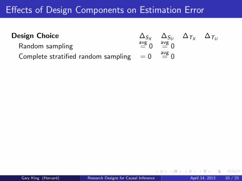
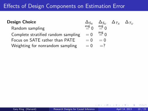
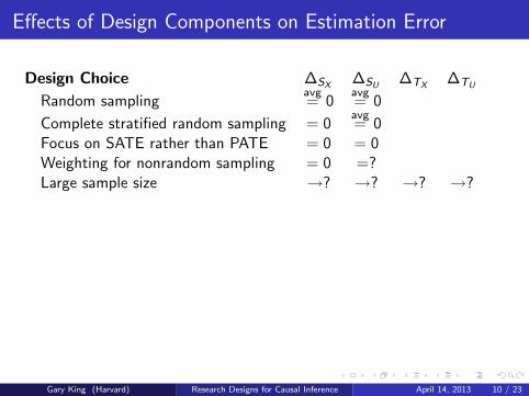
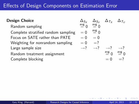
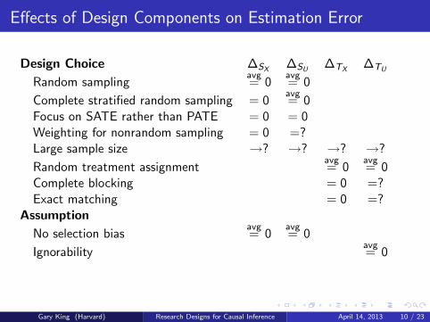
Effects of Design Components on Estimation Error
Design Choice ∆SX∆SU
∆TX∆TU
Random samplingavg= 0
avg= 0
Complete stratified random sampling = 0avg= 0
Focus on SATE rather than PATE = 0 = 0Weighting for nonrandom sampling = 0 =?Large sample size →? →? →? →?
Random treatment assignmentavg= 0
avg= 0
Complete blocking = 0 =?Exact matching = 0 =?
Assumption
No selection biasavg= 0
avg= 0
Ignorabilityavg= 0
No omitted variables = 0
Gary King (Harvard) Research Designs for Causal Inference April 14, 2013 10 / 23

Effects of Design Components on Estimation Error
Design Choice ∆SX∆SU
∆TX∆TU
Random samplingavg= 0
avg= 0
Complete stratified random sampling = 0avg= 0
Focus on SATE rather than PATE = 0 = 0
Weighting for nonrandom sampling = 0 =?Large sample size →? →? →? →?
Random treatment assignmentavg= 0
avg= 0
Complete blocking = 0 =?Exact matching = 0 =?
Assumption
No selection biasavg= 0
avg= 0
Ignorabilityavg= 0
No omitted variables = 0
Gary King (Harvard) Research Designs for Causal Inference April 14, 2013 10 / 23
Effects of Design Components on Estimation Error
Design Choice ∆SX∆SU
∆TX∆TU
Random samplingavg= 0
avg= 0
Complete stratified random sampling = 0avg= 0
Focus on SATE rather than PATE = 0 = 0Weighting for nonrandom sampling = 0 =?
Large sample size →? →? →? →?
Random treatment assignmentavg= 0
avg= 0
Complete blocking = 0 =?Exact matching = 0 =?
Assumption
No selection biasavg= 0
avg= 0
Ignorabilityavg= 0
No omitted variables = 0
Gary King (Harvard) Research Designs for Causal Inference April 14, 2013 10 / 23
Effects of Design Components on Estimation Error
Design Choice ∆SX∆SU
∆TX∆TU
Random samplingavg= 0
avg= 0
Complete stratified random sampling = 0avg= 0
Focus on SATE rather than PATE = 0 = 0Weighting for nonrandom sampling = 0 =?Large sample size →? →? →? →?
Random treatment assignmentavg= 0
avg= 0
Complete blocking = 0 =?Exact matching = 0 =?
Assumption
No selection biasavg= 0
avg= 0
Ignorabilityavg= 0
No omitted variables = 0
Gary King (Harvard) Research Designs for Causal Inference April 14, 2013 10 / 23

Effects of Design Components on Estimation Error
Design Choice ∆SX∆SU
∆TX∆TU
Random samplingavg= 0
avg= 0
Complete stratified random sampling = 0avg= 0
Focus on SATE rather than PATE = 0 = 0Weighting for nonrandom sampling = 0 =?Large sample size →? →? →? →?
Random treatment assignmentavg= 0
avg= 0
Complete blocking = 0 =?Exact matching = 0 =?
Assumption
No selection biasavg= 0
avg= 0
Ignorabilityavg= 0
No omitted variables = 0
Gary King (Harvard) Research Designs for Causal Inference April 14, 2013 10 / 23
Effects of Design Components on Estimation Error
Design Choice ∆SX∆SU
∆TX∆TU
Random samplingavg= 0
avg= 0
Complete stratified random sampling = 0avg= 0
Focus on SATE rather than PATE = 0 = 0Weighting for nonrandom sampling = 0 =?Large sample size →? →? →? →?
Random treatment assignmentavg= 0
avg= 0
Complete blocking = 0 =?
Exact matching = 0 =?Assumption
No selection biasavg= 0
avg= 0
Ignorabilityavg= 0
No omitted variables = 0
Gary King (Harvard) Research Designs for Causal Inference April 14, 2013 10 / 23

Effects of Design Components on Estimation Error
Design Choice ∆SX∆SU
∆TX∆TU
Random samplingavg= 0
avg= 0
Complete stratified random sampling = 0avg= 0
Focus on SATE rather than PATE = 0 = 0Weighting for nonrandom sampling = 0 =?Large sample size →? →? →? →?
Random treatment assignmentavg= 0
avg= 0
Complete blocking = 0 =?Exact matching = 0 =?
Assumption
No selection biasavg= 0
avg= 0
Ignorabilityavg= 0
No omitted variables = 0
Gary King (Harvard) Research Designs for Causal Inference April 14, 2013 10 / 23
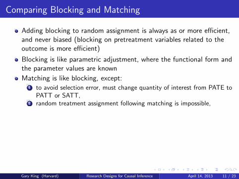
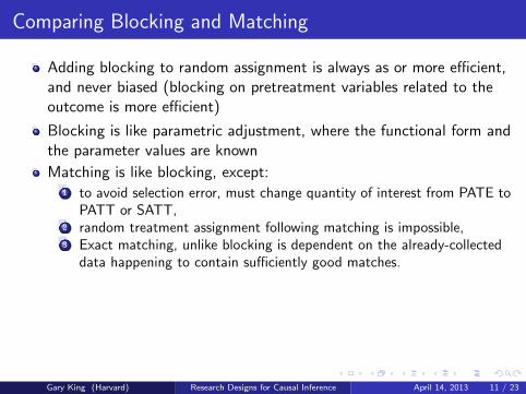
Comparing Blocking and Matching
Adding blocking to random assignment is always as or more efficient,and never biased (blocking on pretreatment variables related to theoutcome is more efficient)
Blocking is like parametric adjustment, where the functional form andthe parameter values are known
Matching is like blocking, except:
1 to avoid selection error, must change quantity of interest from PATE toPATT or SATT,
2 random treatment assignment following matching is impossible,3 Exact matching, unlike blocking is dependent on the already-collected
data happening to contain sufficiently good matches.4 In the worst case scenerio, matching (just like parametric adjustment)
can increase bias (this cannot occur with blocking plus randomassignment)
Adding matching to a parametric model almost always reduces modeldependence and bias, and sometimes variance too
Gary King (Harvard) Research Designs for Causal Inference April 14, 2013 11 / 23

Comparing Blocking and Matching
Adding blocking to random assignment is always as or more efficient,and never biased (blocking on pretreatment variables related to theoutcome is more efficient)
Blocking is like parametric adjustment, where the functional form andthe parameter values are known
Matching is like blocking, except:1 to avoid selection error, must change quantity of interest from PATE to
PATT or SATT,
2 random treatment assignment following matching is impossible,3 Exact matching, unlike blocking is dependent on the already-collected
data happening to contain sufficiently good matches.4 In the worst case scenerio, matching (just like parametric adjustment)
can increase bias (this cannot occur with blocking plus randomassignment)
Adding matching to a parametric model almost always reduces modeldependence and bias, and sometimes variance too
Gary King (Harvard) Research Designs for Causal Inference April 14, 2013 11 / 23
Comparing Blocking and Matching
Adding blocking to random assignment is always as or more efficient,and never biased (blocking on pretreatment variables related to theoutcome is more efficient)
Blocking is like parametric adjustment, where the functional form andthe parameter values are known
Matching is like blocking, except:1 to avoid selection error, must change quantity of interest from PATE to
PATT or SATT,2 random treatment assignment following matching is impossible,
3 Exact matching, unlike blocking is dependent on the already-collecteddata happening to contain sufficiently good matches.
4 In the worst case scenerio, matching (just like parametric adjustment)can increase bias (this cannot occur with blocking plus randomassignment)
Adding matching to a parametric model almost always reduces modeldependence and bias, and sometimes variance too
Gary King (Harvard) Research Designs for Causal Inference April 14, 2013 11 / 23
Comparing Blocking and Matching
Adding blocking to random assignment is always as or more efficient,and never biased (blocking on pretreatment variables related to theoutcome is more efficient)
Blocking is like parametric adjustment, where the functional form andthe parameter values are known
Matching is like blocking, except:1 to avoid selection error, must change quantity of interest from PATE to
PATT or SATT,2 random treatment assignment following matching is impossible,3 Exact matching, unlike blocking is dependent on the already-collected
data happening to contain sufficiently good matches.
4 In the worst case scenerio, matching (just like parametric adjustment)can increase bias (this cannot occur with blocking plus randomassignment)
Adding matching to a parametric model almost always reduces modeldependence and bias, and sometimes variance too
Gary King (Harvard) Research Designs for Causal Inference April 14, 2013 11 / 23

Comparing Blocking and Matching
Adding blocking to random assignment is always as or more efficient,and never biased (blocking on pretreatment variables related to theoutcome is more efficient)
Blocking is like parametric adjustment, where the functional form andthe parameter values are known
Matching is like blocking, except:1 to avoid selection error, must change quantity of interest from PATE to
PATT or SATT,2 random treatment assignment following matching is impossible,3 Exact matching, unlike blocking is dependent on the already-collected
data happening to contain sufficiently good matches.4 In the worst case scenerio, matching (just like parametric adjustment)
can increase bias (this cannot occur with blocking plus randomassignment)
Adding matching to a parametric model almost always reduces modeldependence and bias, and sometimes variance too
Gary King (Harvard) Research Designs for Causal Inference April 14, 2013 11 / 23
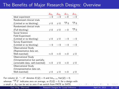
The Benefits of Major Research Designs: Overview
∆SX∆SU
∆TX∆TU
Ideal experiment → 0 → 0 = 0 → 0
Randomized clinicial trials
(Limited or no blocking) 6= 0 6= 0avg= 0
avg= 0
Randomized clinicial trials
(Full blocking) 6= 0 6= 0 = 0avg= 0
Social ScienceField Experiment(Limited or no blocking) 6= 0 6= 0 → 0 → 0
Survey Experiment(Limited or no blocking) → 0 → 0 → 0 → 0
Observational Study(Representative data set,Well-matched) ≈ 0 ≈ 0 ≈ 0 6= 0
Observational Study(Unrepresentative but partially,correctable data, well-matched) ≈ 0 6= 0 ≈ 0 6= 0
Observational Study(Unrepresentative data set,Well-matched) 6= 0 6= 0 ≈ 0 6= 0
For column Q, “→ 0” denotes E (Q) = 0 and limn→∞ Var(Q) = 0,
whereas “avg= 0” indicates zero on average, or E (Q) = 0, for a design with
a small n. ∆S can be set to zero if we switch from PATE to SATE.
Gary King (Harvard) Research Designs for Causal Inference April 14, 2013 12 / 23
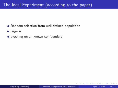
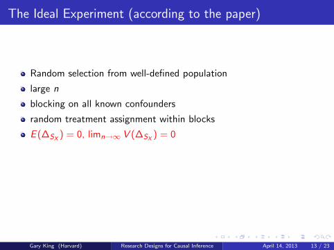
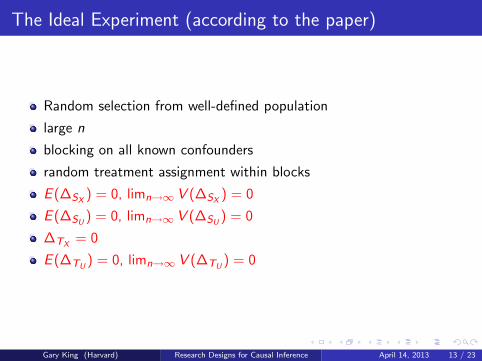
The Ideal Experiment (according to the paper)
Random selection from well-defined population
large n
blocking on all known confounders
random treatment assignment within blocks
E (∆SX) = 0, limn→∞ V (∆SX
) = 0
E (∆SU) = 0, limn→∞ V (∆SU
) = 0
∆TX= 0
E (∆TU) = 0, limn→∞ V (∆TU
) = 0
Gary King (Harvard) Research Designs for Causal Inference April 14, 2013 13 / 23

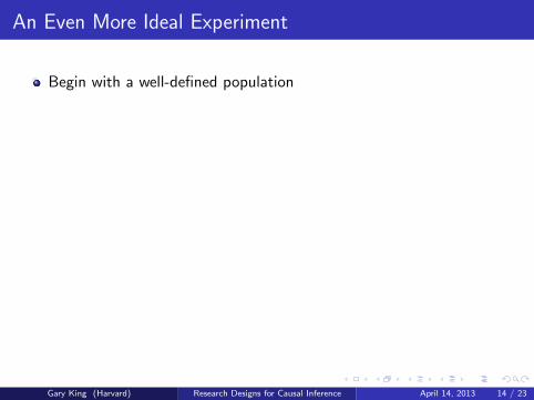
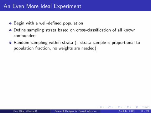
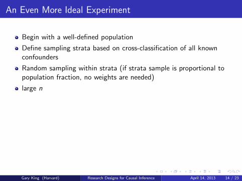
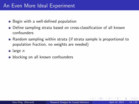
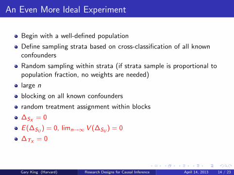
An Even More Ideal Experiment
Begin with a well-defined population
Define sampling strata based on cross-classification of all knownconfounders
Random sampling within strata (if strata sample is proportional topopulation fraction, no weights are needed)
large n
blocking on all known confounders
random treatment assignment within blocks
∆SX= 0
E (∆SU) = 0, limn→∞ V (∆SU
) = 0
∆TX= 0
E (∆TU) = 0, limn→∞ V (∆TU
) = 0
Gary King (Harvard) Research Designs for Causal Inference April 14, 2013 14 / 23

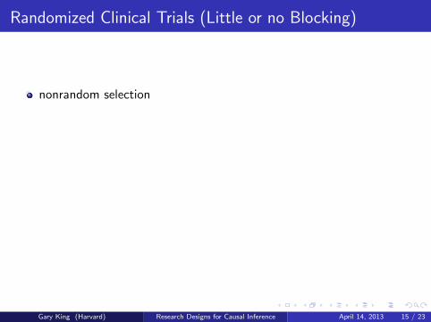
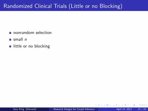
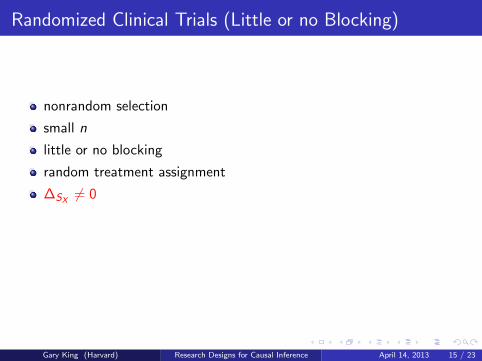
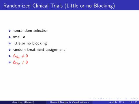
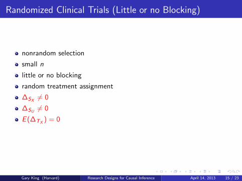
Randomized Clinical Trials (Little or no Blocking)
nonrandom selection
small n
little or no blocking
random treatment assignment
∆SX6= 0
∆SU6= 0
E (∆TX) = 0
E (∆TU) = 0
Gary King (Harvard) Research Designs for Causal Inference April 14, 2013 15 / 23
Randomized Clinical Trials (Little or no Blocking)
nonrandom selection
small n
little or no blocking
random treatment assignment
∆SX6= 0
∆SU6= 0
E (∆TX) = 0
E (∆TU) = 0
Gary King (Harvard) Research Designs for Causal Inference April 14, 2013 15 / 23

Randomized Clinical Trials (Little or no Blocking)
nonrandom selection
small n
little or no blocking
random treatment assignment
∆SX6= 0
∆SU6= 0
E (∆TX) = 0
E (∆TU) = 0
Gary King (Harvard) Research Designs for Causal Inference April 14, 2013 15 / 23
Randomized Clinical Trials (Little or no Blocking)
nonrandom selection
small n
little or no blocking
random treatment assignment
∆SX6= 0
∆SU6= 0
E (∆TX) = 0
E (∆TU) = 0
Gary King (Harvard) Research Designs for Causal Inference April 14, 2013 15 / 23

Randomized Clinical Trials (Little or no Blocking)
nonrandom selection
small n
little or no blocking
random treatment assignment
∆SX6= 0
∆SU6= 0
E (∆TX) = 0
E (∆TU) = 0
Gary King (Harvard) Research Designs for Causal Inference April 14, 2013 15 / 23
Randomized Clinical Trials (Little or no Blocking)
nonrandom selection
small n
little or no blocking
random treatment assignment
∆SX6= 0
∆SU6= 0
E (∆TX) = 0
E (∆TU) = 0
Gary King (Harvard) Research Designs for Causal Inference April 14, 2013 15 / 23
Randomized Clinical Trials (Little or no Blocking)
nonrandom selection
small n
little or no blocking
random treatment assignment
∆SX6= 0
∆SU6= 0
E (∆TX) = 0
E (∆TU) = 0
Gary King (Harvard) Research Designs for Causal Inference April 14, 2013 15 / 23
Randomized Clinical Trials (Little or no Blocking)
nonrandom selection
small n
little or no blocking
random treatment assignment
∆SX6= 0
∆SU6= 0
E (∆TX) = 0
E (∆TU) = 0
Gary King (Harvard) Research Designs for Causal Inference April 14, 2013 15 / 23

Randomized Clinical Trials (Little or no Blocking)
nonrandom selection
small n
little or no blocking
random treatment assignment
∆SX6= 0
∆SU6= 0
E (∆TX) = 0
E (∆TU) = 0
Gary King (Harvard) Research Designs for Causal Inference April 14, 2013 15 / 23

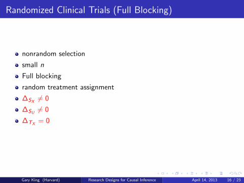
Randomized Clinical Trials (Full Blocking)
nonrandom selection
small n
Full blocking
random treatment assignment
∆SX6= 0
∆SU6= 0
∆TX= 0
E (∆TU) = 0
Gary King (Harvard) Research Designs for Causal Inference April 14, 2013 16 / 23

Randomized Clinical Trials (Full Blocking)
nonrandom selection
small n
Full blocking
random treatment assignment
∆SX6= 0
∆SU6= 0
∆TX= 0
E (∆TU) = 0
Gary King (Harvard) Research Designs for Causal Inference April 14, 2013 16 / 23

Randomized Clinical Trials (Full Blocking)
nonrandom selection
small n
Full blocking
random treatment assignment
∆SX6= 0
∆SU6= 0
∆TX= 0
E (∆TU) = 0
Gary King (Harvard) Research Designs for Causal Inference April 14, 2013 16 / 23

Randomized Clinical Trials (Full Blocking)
nonrandom selection
small n
Full blocking
random treatment assignment
∆SX6= 0
∆SU6= 0
∆TX= 0
E (∆TU) = 0
Gary King (Harvard) Research Designs for Causal Inference April 14, 2013 16 / 23

Randomized Clinical Trials (Full Blocking)
nonrandom selection
small n
Full blocking
random treatment assignment
∆SX6= 0
∆SU6= 0
∆TX= 0
E (∆TU) = 0
Gary King (Harvard) Research Designs for Causal Inference April 14, 2013 16 / 23

Randomized Clinical Trials (Full Blocking)
nonrandom selection
small n
Full blocking
random treatment assignment
∆SX6= 0
∆SU6= 0
∆TX= 0
E (∆TU) = 0
Gary King (Harvard) Research Designs for Causal Inference April 14, 2013 16 / 23

Randomized Clinical Trials (Full Blocking)
nonrandom selection
small n
Full blocking
random treatment assignment
∆SX6= 0
∆SU6= 0
∆TX= 0
E (∆TU) = 0
Gary King (Harvard) Research Designs for Causal Inference April 14, 2013 16 / 23
Randomized Clinical Trials (Full Blocking)
nonrandom selection
small n
Full blocking
random treatment assignment
∆SX6= 0
∆SU6= 0
∆TX= 0
E (∆TU) = 0
Gary King (Harvard) Research Designs for Causal Inference April 14, 2013 16 / 23

Randomized Clinical Trials (Full Blocking)
nonrandom selection
small n
Full blocking
random treatment assignment
∆SX6= 0
∆SU6= 0
∆TX= 0
E (∆TU) = 0
Gary King (Harvard) Research Designs for Causal Inference April 14, 2013 16 / 23

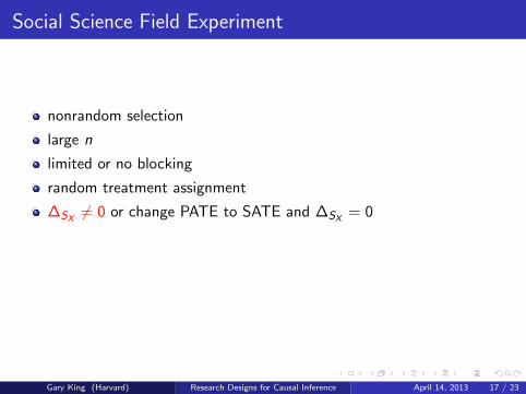
Social Science Field Experiment
nonrandom selection
large n
limited or no blocking
random treatment assignment
∆SX6= 0 or change PATE to SATE and ∆SX
= 0
∆SU6= 0 or change PATE to SATE and ∆SU
= 0
E (∆TX) = 0, limn→∞ V (∆TX
) = 0
E (∆TU) = 0, limn→∞ V (∆TU
) = 0
Gary King (Harvard) Research Designs for Causal Inference April 14, 2013 17 / 23

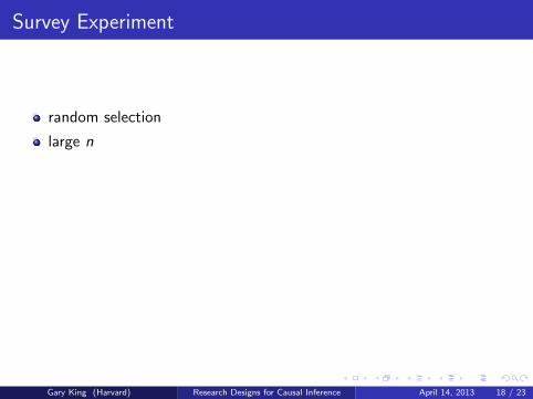
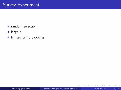
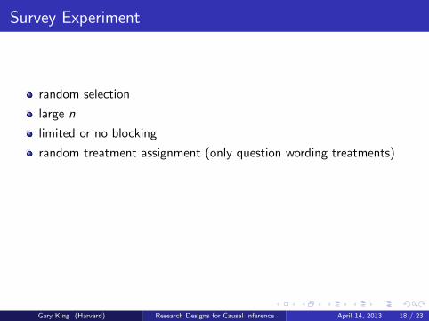
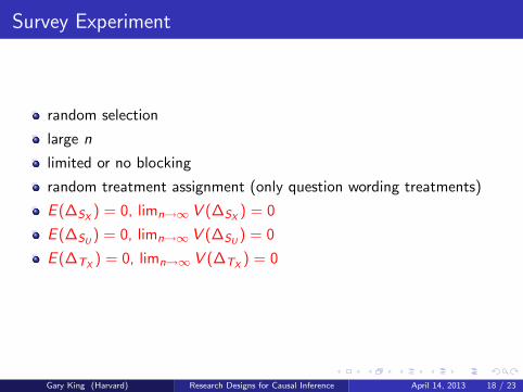
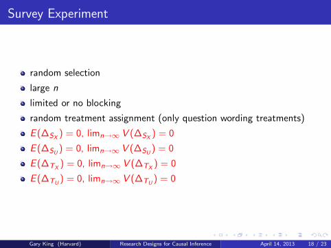
Survey Experiment
random selection
large n
limited or no blocking
random treatment assignment (only question wording treatments)
E (∆SX) = 0, limn→∞ V (∆SX
) = 0
E (∆SU) = 0, limn→∞ V (∆SU
) = 0
E (∆TX) = 0, limn→∞ V (∆TX
) = 0
E (∆TU) = 0, limn→∞ V (∆TU
) = 0
Gary King (Harvard) Research Designs for Causal Inference April 14, 2013 18 / 23
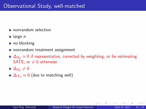
Observational Study, well-matched
nonrandom selection
large n
no blocking
nonrandom treatment assignment
∆SX≈ 0 if representative, corrected by weighting, or for estimating
SATE; or 6= 0 otherwise
∆SU6= 0
∆TX≈ 0 (due to matching well)
∆TU6= 0 except by assumption
Gary King (Harvard) Research Designs for Causal Inference April 14, 2013 19 / 23

What is the Best Design?
The ideal design is rarely feasible
the Achilles heal of experimental studies: ∆S and small n
the Achilles heal of observational studies: ∆U
Each design accomodates best to the applications for which it wasdesigned
Effort in experimental studies: random assignment
Effort in observational studies: measuring and adjusting for X (viamatching or modeling)
Gary King (Harvard) Research Designs for Causal Inference April 14, 2013 20 / 23
Fallacies in Experimental Research
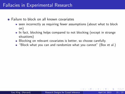
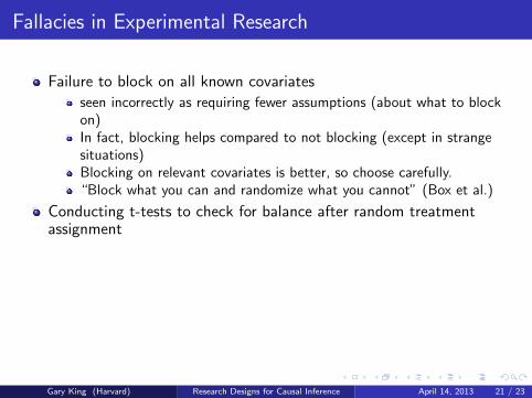
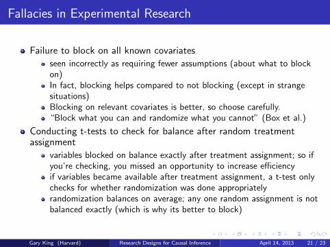
Failure to block on all known covariates
seen incorrectly as requiring fewer assumptions (about what to blockon)In fact, blocking helps compared to not blocking (except in strangesituations)Blocking on relevant covariates is better, so choose carefully.“Block what you can and randomize what you cannot” (Box et al.)
Conducting t-tests to check for balance after random treatmentassignment
variables blocked on balance exactly after treatment assignment; so ifyou’re checking, you missed an opportunity to increase efficiencyif variables became available after treatment assignment, a t-test onlychecks for whether randomization was done appropriatelyrandomization balances on average; any one random assignment is notbalanced exactly (which is why its better to block)
Gary King (Harvard) Research Designs for Causal Inference April 14, 2013 21 / 23

Fallacies in Experimental Research
Failure to block on all known covariates
seen incorrectly as requiring fewer assumptions (about what to blockon)
In fact, blocking helps compared to not blocking (except in strangesituations)Blocking on relevant covariates is better, so choose carefully.“Block what you can and randomize what you cannot” (Box et al.)
Conducting t-tests to check for balance after random treatmentassignment
variables blocked on balance exactly after treatment assignment; so ifyou’re checking, you missed an opportunity to increase efficiencyif variables became available after treatment assignment, a t-test onlychecks for whether randomization was done appropriatelyrandomization balances on average; any one random assignment is notbalanced exactly (which is why its better to block)
Gary King (Harvard) Research Designs for Causal Inference April 14, 2013 21 / 23
Fallacies in Experimental Research
Failure to block on all known covariates
seen incorrectly as requiring fewer assumptions (about what to blockon)In fact, blocking helps compared to not blocking (except in strangesituations)
Blocking on relevant covariates is better, so choose carefully.“Block what you can and randomize what you cannot” (Box et al.)
Conducting t-tests to check for balance after random treatmentassignment
variables blocked on balance exactly after treatment assignment; so ifyou’re checking, you missed an opportunity to increase efficiencyif variables became available after treatment assignment, a t-test onlychecks for whether randomization was done appropriatelyrandomization balances on average; any one random assignment is notbalanced exactly (which is why its better to block)
Gary King (Harvard) Research Designs for Causal Inference April 14, 2013 21 / 23

Fallacies in Experimental Research
Failure to block on all known covariates
seen incorrectly as requiring fewer assumptions (about what to blockon)In fact, blocking helps compared to not blocking (except in strangesituations)Blocking on relevant covariates is better, so choose carefully.
“Block what you can and randomize what you cannot” (Box et al.)
Conducting t-tests to check for balance after random treatmentassignment
variables blocked on balance exactly after treatment assignment; so ifyou’re checking, you missed an opportunity to increase efficiencyif variables became available after treatment assignment, a t-test onlychecks for whether randomization was done appropriatelyrandomization balances on average; any one random assignment is notbalanced exactly (which is why its better to block)
Gary King (Harvard) Research Designs for Causal Inference April 14, 2013 21 / 23
Fallacies in Experimental Research
Failure to block on all known covariates
seen incorrectly as requiring fewer assumptions (about what to blockon)In fact, blocking helps compared to not blocking (except in strangesituations)Blocking on relevant covariates is better, so choose carefully.“Block what you can and randomize what you cannot” (Box et al.)
Conducting t-tests to check for balance after random treatmentassignment
variables blocked on balance exactly after treatment assignment; so ifyou’re checking, you missed an opportunity to increase efficiencyif variables became available after treatment assignment, a t-test onlychecks for whether randomization was done appropriatelyrandomization balances on average; any one random assignment is notbalanced exactly (which is why its better to block)
Gary King (Harvard) Research Designs for Causal Inference April 14, 2013 21 / 23

Fallacies in Experimental Research
Failure to block on all known covariates
seen incorrectly as requiring fewer assumptions (about what to blockon)In fact, blocking helps compared to not blocking (except in strangesituations)Blocking on relevant covariates is better, so choose carefully.“Block what you can and randomize what you cannot” (Box et al.)
Conducting t-tests to check for balance after random treatmentassignment
variables blocked on balance exactly after treatment assignment; so ifyou’re checking, you missed an opportunity to increase efficiency
if variables became available after treatment assignment, a t-test onlychecks for whether randomization was done appropriatelyrandomization balances on average; any one random assignment is notbalanced exactly (which is why its better to block)
Gary King (Harvard) Research Designs for Causal Inference April 14, 2013 21 / 23

Fallacies in Experimental Research
Failure to block on all known covariates
seen incorrectly as requiring fewer assumptions (about what to blockon)In fact, blocking helps compared to not blocking (except in strangesituations)Blocking on relevant covariates is better, so choose carefully.“Block what you can and randomize what you cannot” (Box et al.)
Conducting t-tests to check for balance after random treatmentassignment
variables blocked on balance exactly after treatment assignment; so ifyou’re checking, you missed an opportunity to increase efficiencyif variables became available after treatment assignment, a t-test onlychecks for whether randomization was done appropriately
randomization balances on average; any one random assignment is notbalanced exactly (which is why its better to block)
Gary King (Harvard) Research Designs for Causal Inference April 14, 2013 21 / 23
Fallacies in Experimental Research
Failure to block on all known covariates
seen incorrectly as requiring fewer assumptions (about what to blockon)In fact, blocking helps compared to not blocking (except in strangesituations)Blocking on relevant covariates is better, so choose carefully.“Block what you can and randomize what you cannot” (Box et al.)
Conducting t-tests to check for balance after random treatmentassignment
variables blocked on balance exactly after treatment assignment; so ifyou’re checking, you missed an opportunity to increase efficiencyif variables became available after treatment assignment, a t-test onlychecks for whether randomization was done appropriatelyrandomization balances on average; any one random assignment is notbalanced exactly (which is why its better to block)
Gary King (Harvard) Research Designs for Causal Inference April 14, 2013 21 / 23
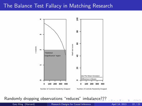
The Balance Test Fallacy in Matching Research
0 100 200 300 400
01
23
4
"Statistical
insignificance" region
0 100 200 300 400
01
23
4
Number of Controls Randomly Dropped
t−st
atis
tic
0 100 200 300 400
020
4060
8010
0Difference in Means
0 100 200 300 400
020
4060
8010
0
Number of Controls Randomly Dropped
Mat
h te
st s
core
QQ Plot Mean Deviation
Randomly dropping observations “reduces” imbalance???Gary King (Harvard) Research Designs for Causal Inference April 14, 2013 22 / 23

The Balance Test Fallacy: Explanation
hypothesis tests are a function of balance AND power; we only wantto measure balance
for SATE, PATE, or SPATE, balance is a characteristic of the sample,not some superpopulation; so no need to make an inference
Simple linear model (for intution):
Suppose E (Y | T ,X ) = θ + Tβ + XγBias in coefficient on T from regressing Y on T (without X ):E (β̂ − β | T ,X ) = Gγ (where G are coefficients from a regression Xon a constant and T )Imbalance is due to G only.If G = 0, bias=0If G 6= 0, bias can be any size due to γIf you cannot control G (and we don’t usually try to minimize γ so wedon’t cook the books), then G must be reduced without limit.
No threshold level is safe.
Gary King (Harvard) Research Designs for Causal Inference April 14, 2013 23 / 23
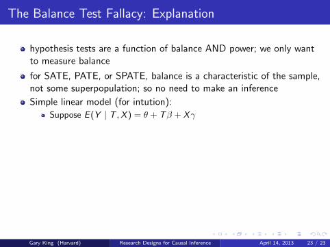
The Balance Test Fallacy: Explanation
hypothesis tests are a function of balance AND power; we only wantto measure balance
for SATE, PATE, or SPATE, balance is a characteristic of the sample,not some superpopulation; so no need to make an inference
Simple linear model (for intution):
Suppose E (Y | T ,X ) = θ + Tβ + Xγ
Bias in coefficient on T from regressing Y on T (without X ):E (β̂ − β | T ,X ) = Gγ (where G are coefficients from a regression Xon a constant and T )Imbalance is due to G only.If G = 0, bias=0If G 6= 0, bias can be any size due to γIf you cannot control G (and we don’t usually try to minimize γ so wedon’t cook the books), then G must be reduced without limit.
No threshold level is safe.
Gary King (Harvard) Research Designs for Causal Inference April 14, 2013 23 / 23

The Balance Test Fallacy: Explanation
hypothesis tests are a function of balance AND power; we only wantto measure balance
for SATE, PATE, or SPATE, balance is a characteristic of the sample,not some superpopulation; so no need to make an inference
Simple linear model (for intution):
Suppose E (Y | T ,X ) = θ + Tβ + XγBias in coefficient on T from regressing Y on T (without X ):E (β̂ − β | T ,X ) = Gγ (where G are coefficients from a regression Xon a constant and T )
Imbalance is due to G only.If G = 0, bias=0If G 6= 0, bias can be any size due to γIf you cannot control G (and we don’t usually try to minimize γ so wedon’t cook the books), then G must be reduced without limit.
No threshold level is safe.
Gary King (Harvard) Research Designs for Causal Inference April 14, 2013 23 / 23
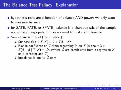
The Balance Test Fallacy: Explanation
hypothesis tests are a function of balance AND power; we only wantto measure balance
for SATE, PATE, or SPATE, balance is a characteristic of the sample,not some superpopulation; so no need to make an inference
Simple linear model (for intution):
Suppose E (Y | T ,X ) = θ + Tβ + XγBias in coefficient on T from regressing Y on T (without X ):E (β̂ − β | T ,X ) = Gγ (where G are coefficients from a regression Xon a constant and T )Imbalance is due to G only.
If G = 0, bias=0If G 6= 0, bias can be any size due to γIf you cannot control G (and we don’t usually try to minimize γ so wedon’t cook the books), then G must be reduced without limit.
No threshold level is safe.
Gary King (Harvard) Research Designs for Causal Inference April 14, 2013 23 / 23

The Balance Test Fallacy: Explanation
hypothesis tests are a function of balance AND power; we only wantto measure balance
for SATE, PATE, or SPATE, balance is a characteristic of the sample,not some superpopulation; so no need to make an inference
Simple linear model (for intution):
Suppose E (Y | T ,X ) = θ + Tβ + XγBias in coefficient on T from regressing Y on T (without X ):E (β̂ − β | T ,X ) = Gγ (where G are coefficients from a regression Xon a constant and T )Imbalance is due to G only.If G = 0, bias=0
If G 6= 0, bias can be any size due to γIf you cannot control G (and we don’t usually try to minimize γ so wedon’t cook the books), then G must be reduced without limit.
No threshold level is safe.
Gary King (Harvard) Research Designs for Causal Inference April 14, 2013 23 / 23

The Balance Test Fallacy: Explanation
hypothesis tests are a function of balance AND power; we only wantto measure balance
for SATE, PATE, or SPATE, balance is a characteristic of the sample,not some superpopulation; so no need to make an inference
Simple linear model (for intution):
Suppose E (Y | T ,X ) = θ + Tβ + XγBias in coefficient on T from regressing Y on T (without X ):E (β̂ − β | T ,X ) = Gγ (where G are coefficients from a regression Xon a constant and T )Imbalance is due to G only.If G = 0, bias=0If G 6= 0, bias can be any size due to γ
If you cannot control G (and we don’t usually try to minimize γ so wedon’t cook the books), then G must be reduced without limit.
No threshold level is safe.
Gary King (Harvard) Research Designs for Causal Inference April 14, 2013 23 / 23

The Balance Test Fallacy: Explanation
hypothesis tests are a function of balance AND power; we only wantto measure balance
for SATE, PATE, or SPATE, balance is a characteristic of the sample,not some superpopulation; so no need to make an inference
Simple linear model (for intution):
Suppose E (Y | T ,X ) = θ + Tβ + XγBias in coefficient on T from regressing Y on T (without X ):E (β̂ − β | T ,X ) = Gγ (where G are coefficients from a regression Xon a constant and T )Imbalance is due to G only.If G = 0, bias=0If G 6= 0, bias can be any size due to γIf you cannot control G (and we don’t usually try to minimize γ so wedon’t cook the books), then G must be reduced without limit.
No threshold level is safe.
Gary King (Harvard) Research Designs for Causal Inference April 14, 2013 23 / 23

The Balance Test Fallacy: Explanation
hypothesis tests are a function of balance AND power; we only wantto measure balance
for SATE, PATE, or SPATE, balance is a characteristic of the sample,not some superpopulation; so no need to make an inference
Simple linear model (for intution):
Suppose E (Y | T ,X ) = θ + Tβ + XγBias in coefficient on T from regressing Y on T (without X ):E (β̂ − β | T ,X ) = Gγ (where G are coefficients from a regression Xon a constant and T )Imbalance is due to G only.If G = 0, bias=0If G 6= 0, bias can be any size due to γIf you cannot control G (and we don’t usually try to minimize γ so wedon’t cook the books), then G must be reduced without limit.
No threshold level is safe.
Gary King (Harvard) Research Designs for Causal Inference April 14, 2013 23 / 23