research article modeling and finite-time walking control
TRANSCRIPT
Research ArticleModeling and Finite-Time Walking Control ofa Biped Robot with Feet
Juan E Machado Heacutector M Becerra and Moacutenica Moreno Rocha
Centro de Investigacion en Matematicas (CIMAT) AC Jalisco SN Colonia Valenciana 36240 Guanajuato GTO Mexico
Correspondence should be addressed to Hector M Becerra hectorbecerracimatmx
Received 11 August 2015 Accepted 18 October 2015
Academic Editor Guangming Xie
Copyright copy 2015 Juan E Machado et al This is an open access article distributed under the Creative Commons AttributionLicense which permits unrestricted use distribution and reproduction in any medium provided the original work is properlycited
This paper addresses the problemofmodeling and controlling a planar biped robot with six degrees of freedomwhich are generatedby the interaction of seven links including feet The biped is modeled as a hybrid dynamical system with a fully actuated single-support phase and an instantaneous double-support phase The mathematical modeling is detailed in the first part of the paperIn the second part we present the synthesis of a controller based on virtual constraints which are codified in an output functionthat allows defining a local diffeomorphism to linearize the robot dynamics Finite-time convergence of the output to the originensures a collision between the swing foot and the ground with an appropriate configuration for the robot to give a step forwardThe components of the output track adequate references that encode a walking pattern Finite-time convergence of the trackingerrors is enforced by using second-order slidingmode controlThemain contribution of the paper is an evaluation and comparisonof discontinuous and continuous sliding mode control in the presence of parametric uncertainty and external disturbances Therobot model and the synthesized controller are evaluated through numerical simulations
1 Introduction
The study of walking robots is a research area of greatscientific and technological interest [1] A particular class ofwalking robots are bipeds which are characterized for theirmobility from two legs The kinematics and dynamics of thiskind of robots are complex and the synthesis of efficient androbust controllers to achieve stable walking is a challengingtask [2] This paper studies a planar biped robot that consistsof seven links two femurs two tibias two feet and one torsoThis structure of biped robot is the simplest that approxi-mately reproduces the mechanism of human walking [2 3]
The modeling of biped robots as a system of multiplependulums has been addressed from the simplest case in [4]where the robot is represented by only 3 links with no kneesnor feet In order to analyze a model more similar to thehuman anatomy the biped robot of 5 links has been one ofthe most studied ones in the literature for instance in [5 6]In such case the robot has knees but not feet
In the literature several models of planar bipeds havebeen considered without feet which means that the contact
with the ground is assumed to be punctual see for instance[5 6] However feet play an important role in the wholewalking process Feet allow the robot to improve balanceproviding a supporting surface to distribute its weightExamples of bipeds with feet can be found in [2 3 6] Inthe aforementioned references the modeled robots are bipedswhose motion is constrained to the sagitttal plane This is avalid assumption in a biped robot since the dynamics in thesagittal plane is basically decoupled from the dynamics in thefrontal plane [2] Besides essential components of the bipedalwalking can be observed in the sagittal plane
Different control techniques have been used for thewalking control of biped robots High gain linear control isproposed in [7] where the authors prove that exponentialconvergence of the closed-loop system is achieved Howevera high gain proportional-derivative control is not feasibledue to the large magnitude of the generated control inputsExtensive research on passivity-based control of biped robotsis summarized in [8] where energetic functions are exploitedto formulate a walking controller robust to some externaldisturbances but not to parametric uncertainty It is well
Hindawi Publishing CorporationMathematical Problems in EngineeringVolume 2015 Article ID 963496 17 pageshttpdxdoiorg1011552015963496
2 Mathematical Problems in Engineering
known that classical sliding mode control is a robust controltechnique [9] able to stabilize electromechanical systemssubject to external matched disturbances and parametricuncertainty Such properties have been exploited for therobust control of biped robots in [6 10 11] In [6] a first-ordersliding mode control is proposed for an underactuated bipedand its performance is evaluated for external disturbancesThe authors of [10] compare a classical sliding mode con-troller with a pure computed torque controller concludingthe superiority of the first one The robot model of [11]includes a double-support phase in which a sliding modecontroller regulates the robotrsquos motion
The previously referred to walking controllers usingsliding mode control present the problem of the classicalapproach the undesirable effect of chattering [9] Second-order sliding mode control has been proposed in order toreduce the chattering effect of the classical approach [12]This kind of sliding mode control has been studied for robustcontrol of second-order systems to achieve stabilization infinite-time in particular for double integrator systems [1314] Finite-time control of the bipedrsquos state variables is animportant feature in order to achieve a stable walking cycleall bipedrsquos state variables must converge to desired valuesbefore the occurrence of an impact between the swing footand the ground at each step In [15] the authors propose anonlinear control with finite-time convergence which hasbeen applied for biped robots in [4 5] Second-order slidingmodes can be achieved by using a discontinuous [13] ora continuous [14] control law Both approaches have beenproposed for the walking control of biped robots [16 17]however a comparison and robustness evaluation of bothapproaches have not been carried out
In this paper we detail the mathematical model of a 7-link biped robot including feet The biped is modeled asa hybrid system with a continuous fully actuated single-support phase and an instantaneous double-support phasemodeled as a discontinuous transition of the velocities whenthe swing foot collides with the ground The validity of themodel is verified from the dynamic constraint given by thecenter of pressure We propose a particular set of outputsto be controlled which allows us to design a controller thattransforms themodel of the biped into a linear form Second-order sliding mode control is then used over the linearizedsystem to ensure robust reference tracking in finite-timeThe main contribution of the paper is an evaluation andcomparison of both discontinuous and continuous second-order slidingmode approaches in terms of robustness againstparametric uncertainty and external disturbances To thisend the complete model of the biped and the proposedwalking control have been implemented in simulation usingPython
The paper is organized as follows Section 2 summarizesthe modeling hypotheses and states the addressed problemSection 3 details the mathematical model of the 7-link bipedrobot In Section 4 we describe the synthesis of a walkingcontrol for the 7-link biped Section 5 shows results ofthe closed-loop systemrsquos performance through simulationsusing the derived mathematical model In Section 6 we giveconclusions and discuss some future work
1205911
1205912
1205913
1205914
1205915
1205916
ℬ0
ℬ1
ℬ2
ℬ3
ℬ4
ℬ5
ℬ6
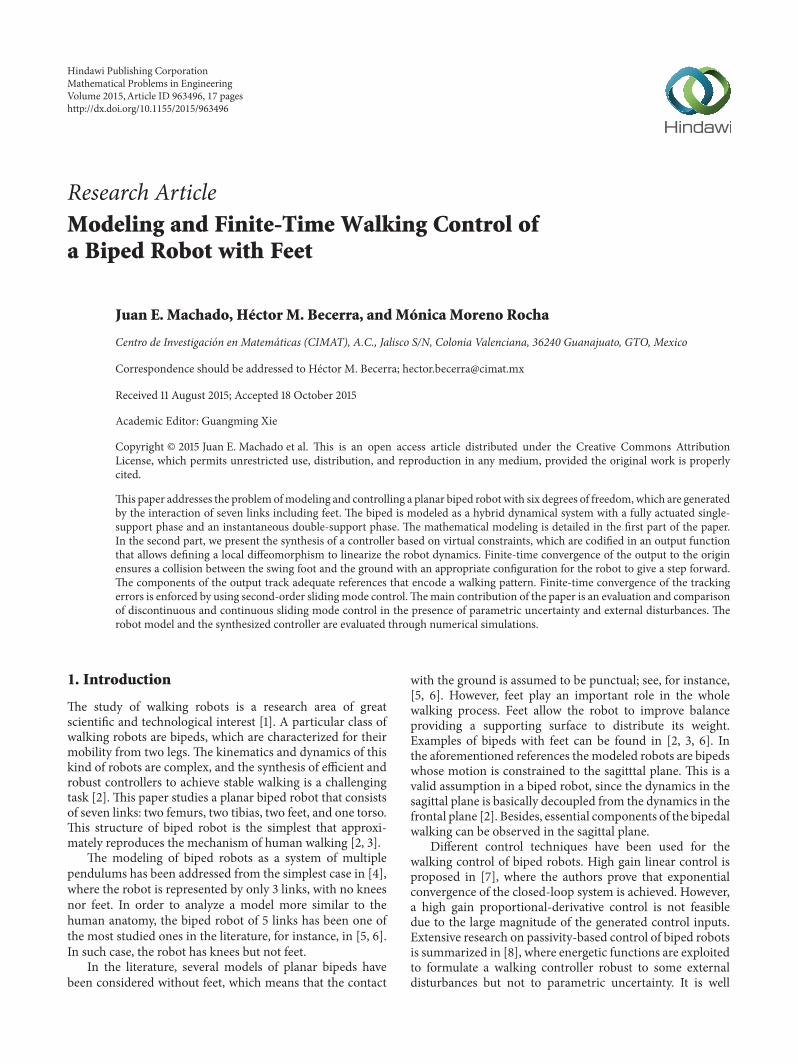
Figure 1 Scheme of the 7-link biped robot showing the links(B0 B
6) and torques (120591
1 120591
6)
2 Modeling Hypotheses andProblem Statement
In this section we enlist a set of modeling hypotheses andwe describe the main problem addressed in the paper Thefollowing hypotheses regarding the robot are assumed
(HR1) It consists of 7 links of cylindrical geometry andhomogeneous density distributed in a torso and twoidentical legs each leg is composed of two links andone foot (see Figure 1)(HR2) It is planar and its motion is constrained to thesagittal plane which is identified with a vertical 119909119910-plane(HR3) The 6 joints (2 ankles 2 knees and 2 hips) areone-degree-of-freedom rotational frictionless joints
Additionally we assume that the bipedal walking satisfiesthe following hypotheses
(HW1) It consists of two successive phases a fullyactuated single-support phase (robot standing onone leg) and an instantaneous double-support phase(both feet on the ground)(HW2) During the single-support phase the stance legremains planar on the ground and without slipping(HW3) In each step the swing leg moves forward frombehind the stance leg to the front(HW4) The walking is performed from left to right ona horizontal straight line representing the ground
In this paper we address the problem of deriving a modelof a biped robot accomplishing the aforementioned hypothe-ses From this model we design a walking controller robustagainst parametric uncertainty and external disturbancesable to achieve convergence of a set of selected outputs infinite-time before the occurrence of an impact of the swingfoot with the ground for each step of the robot
Mathematical Problems in Engineering 3
z0
x0
y0
O0
q1
q2
q3
q4
q5
q6
P1
P2
P3
P4
P5
Figure 2 Scheme of the 7-link biped robot showing the jointsrsquopositions (P
1 P
5) angles of configuration (119902
1 119902
6) and fixed
reference frameF0with origin 119874
0
3 Model of a 7-Link Biped Robot
In this section we detail the aspects related to the modelof the biped robot under the assumptions described in theprevious section The model is developed in two parts Firstthe robot dynamics in the single-support phase ismodeled bya set of differential equations with inputs which are obtainedfrom the Euler-Lagrange formulation Second a model ofthe collision of the swing foot and the ground is presentedas a set of algebraic constraints [2 5] The two-phase modelrepresenting the walking cycle of the 7-link biped is thenwritten as a hybrid nonlinear system with impulsive effects[4 5]
31 LagrangianDynamics of the Robot Each joint of the robothas a torque 120591
119894associated as shown in Figure 1 Then the
vector of input torques can be written as 120591 = (1205911 120591
6)
Let us define a vector of generalized coordinates q =
(1199021 119902
6) which represents the robotrsquos configurationThus
the robot has 6 degrees of freedom and is fully actuatedThe angular positions 119902
119894are measured as shown in Figure 2
with positive angles in a counterclockwise sense The Euler-Lagrange equations can be written as follows
119889
119889119905
120597L
120597q119894minus
120597L
120597q119894= 120583119894
for 119894 = 1 6 (1)
where L(q q) = K(q q) minus P(q) is the differencebetween the kinetic energy K and the potential energyP due to the gravity force 120583
119894is the generalized force
for each B119894 The kinetic energy is given by K(q q) =
sum
6
119894=1((12)119898
119894Q119879119894Q119894+ (12)119895
119894119902
2
119894) where Q
119894is the center of
mass and 119895119894= (112)119898
119894(2119897119894)
2 is the moment of inertia ofeach B
119894(see Appendix A) The potential energy is given by
P(q) = minussum
6
119894=1(119898119894g119879Q119894) where g = (0 minus119892
119910 0) with 119892
119910
the gravitational constant Euler-Lagrange equations (1) for
the studied robotic system can be expressed in the second-order form [18]
B (q) q + C (q q) q + G (q) = A120591 (2)
where B(q) is a positive definite symmetric matrix of 6 times 6known as matrix of inertia the vector fields C(q q) andG(q)include the centrifugal Coriolis and gravitational effects onthe robot 120591 is the vector of input torques and the matrixA isin1198726times6(R) relates 120591with the vector of generalized forces 120583The
matrixA is invertible given that the robot is fully actuated SeeAppendix B for details of the terms involved in (2) Model (2)can be expressed in a state-space form as the following systemof 12 first-order differential equations
119889
119889119905
x = [q
Bminus1 (q) (u minus C (q q) q minus G (q))]
= f (x) + g (x) u
(3)
where x = (q q) is the state vector and u = A120591 = 120583 is thecontrol variable The state-space of the system is defined asX = x isin R12 | q isin (minus120587 120587)6 q isin R6 and q lt 119872 lt infinwith119872 a positive scalar Since we will introduce conditionsfor collision of the swing foot with the ground the state-spaceis actually reduced to a subset of X of physically admissibleconfigurations
32 Collision Model The instantaneous double-supportphase is modeled as a collision between the swing foot andthe ground To obtain a collision model we consider thefollowing hypotheses [19]
(HC1)The impact ismodeled as a contact between tworigid bodies(HC2) The contact takes an infinitesimal time period(HC3) The swing foot makes a strictly parallel contactwith the ground and there is no rebound and noslipping of the foot(HC4) The stance leg lifts from the ground withoutinteraction(HC5) The external forces (eg ground reaction)during the collision can be modeled as impulses(HC6) The actuators (joint motors) cannot generateimpulses hence they can be neglected in the collisionmodel(HC7) Due to the impulsive forces the joint velocitiesmight present a discontinuous change not so in theconfiguration
Since we consider a robot with feet the contact of theswing foot with the ground implies the application of adistribution of forces in the sole of the foot However avalid simplification is to consider one resultant force and anexternal torque both acting in the swing footrsquos ankle at theinstant of contact [2] Let us define P
5(q) as the position
of the swing footrsquos ankle with respect to the frame F0and
4 Mathematical Problems in Engineering
P120579(q) = (0 0 0 0 119902
5 0) as the absolute angle of the swing foot
measured as shown in Figure 2 We can introduce the effectof the impulsive external forces due to the collision in (2) asfollows [20]
B (q) q + C (q q) q + G (q) = A120591 + J1198791198755
120575F119890+ J119879119875120579
120575120591119890 (4)
where J1198755
= 120597P5(q)120597q is a 2 times 6 full rank matrix and
J119875120579
= 120597P120579(q)120597q is a vector inR6 (these matrices are given in
Appendix A) 120575F119890and 120575120591
119890are vector-valued functions in R2
andR respectively which denote the resultant external forceand torque acting in the swing footrsquos ankle at the moment ofimpact (in form of Dirac delta functions) Considering (HC2)the integral of (4) during the infinitesimal time of the collisionis given by
B (q) (q+ minus qminus) = J1198791198755
F119890+ J119879119875120579
120591119890 (5)
where F119890= int
119905+
119905minus120575F119890(120591) 119889120591 120591
119890= int
119905+
119905minus120575120591119890(120591) 119889120591 and qplusmn =
q(119905plusmn) 119905minus and 119905+ being the instants before and after impactwhich satisfy 119905+ minus 119905minus rarr 0 Recall that by (HC7) the robotconfiguration does not change during the collision thus q+ =q(119905minus) = q(119905+) From (5) the goal is to compute q+ knowing qand qminus However F
119890and 120591119890are also unknown Since in 119905+ the
swing leg becomes the stance leg hypothesis (HW2) impliesthat the translational and rotational velocities of the stancefoot are null Thus after the impact it is satisfied that
P5(119905
+) = J1198755
q+ = 0
P120579(119905
+) = J119875120579
q+ = 0(6)
Using (5) and (6) we can write a linear system to solve for q+F119890 and 120591
119890 which can be expressed as follows
Π
[
[
[
[
q+
F119890
120591119890
]
]
]
]
= [
B (q) qminus
03times6
] (7)
where
Π =
[
[
[
[
B (q) minusJ1198791198755
minusJ119879119875120579
J1198755
02times2
02times1
J119875120579
01times2
01times1
]
]
]
]
(8)
Proposition 1 Linear system (7) has a single solution
This proposition whose proof is given in Appendix Cestablishes that we can always compute a solution of (7)in terms of qminus The following lemma specifies the explicitsolution of system (7)
Lemma2 Theclosed-form of the solution of system (7) is givenby
F119890= minusMminus1
1J1198755
qminus
120591119890= minusMminus1
2J119875120579
qminus
q+ = minusBminus1 (q) J1198791198755
Mminus11J1198755
qminus
minus (Bminus1 (q) J119879119875120579
Mminus12J119875120579
minus I6times6) qminus
= Δ2qminus
(9)
where M1= J1198755
Bminus1(q)J1198791198755
and M2= J119875120579
Bminus1(q)J119879119875120579
arenonsingular matrices
Proof Solving for q+ in (5) we have
q+ = Bminus1 (q) (J1198791198755
F119890+ J119879119875120579
120591119890) + qminus (10)
Premultiplying (10) by J1198755
and by J119875120579
we obtain
J1198755
q+ = J1198755
Bminus1 (q) (J1198791198755
F119890+ J119879119875120579
120591119890) + J1198755
qminus
J119875120579
q+ = J119875120579
Bminus1 (q) (J1198791198755
F119890+ J119879119875120579
120591119890) + J119875120579
qminus(11)
respectively Using (6) the left-hand sides of (11) become nullBesides due to the form of J
1198755
and J119875120579
given in Appendix A itcan be verified that J
1198755
Bminus1(q)J119879119875120579
= 02times1
and (J119875120579
Bminus1(q)J1198791198755
)
119879=
01times2
which simplify the expressions in (11) to
0 = J1198755
Bminus1 (q) J1198791198755
F119890+ J1198755
qminus = M1F119890+ J1198755
qminus
0 = J119875120579
Bminus1 (q) J119879119875120579
120591119890+ J119875120579
qminus = M2120591119890+ J119875120579
qminus(12)
implying that
F119890= minusMminus1
1J1198755
qminus
120591119890= minusMminus1
2J119875120579
qminus(13)
Since B(q) is a positive definite matrix and J1198755
and J119875120579
arefull rank matrices it can be verified that J
1198755
Bminus1(q)J1198791198755
= M1
and J119875120579
Bminus1(q)J119879119875120579
= M2are symmetric positive matrices
and consequently they are invertible Finally replacing thesolution for F
119890and 120591
119890in (10) we obtain
q+ = minusBminus1 (q) J1198791198755
Mminus11J1198755
qminus
minus (Bminus1 (q) J119879119875120579
Mminus12J119875120579
minus I6times6) qminus = Δ
2qminus
(14)
This result along with the fact that q+ = qminus = q allows usto determine the restart condition of the continuous dynam-ics in (3) To do so we introduce a change of coordinatesthat represents the transformation of the swing leg to thestance leg and vice versa By symmetry of the legs this isdone by relabeling the coordinates of q and q We express
Mathematical Problems in Engineering 5
that relabeling as a matrix D isin 1198725times5(R) acting on the first
five coordinates of q and q such that DD = I5times5
Notice thatthe last coordinates of q and q corresponding to the positionand velocity of the torso are not affected because they areindependent of the legs disposal Finally the collision modelwhich gives the robot state after the impact x+ = (q q+) interms of xminus = (q qminus) can be written as
x+ = [[D 05times1] q
[D 05times4]Δ2qminus
] = Δ (xminus) (15)
where Δ2is defined in (9) Since the calculation is direct an
explicit expression of Δ is not given However the implicitfunction theorem implies thatΔ is as smooth as the entries ofΠ in (7) Hence we can conclude that Δ is analytic in xminus
33 Complete Model as a Hybrid System Now we describea form to represent the complete model of the biped takinginto account the continuous part given by (3) and thediscrete part given by (15) This kind of hybrid systems canbe described as a system with impulsive effects [21] Thefollowing proposition establishes the complete model of thebiped robot
Proposition 3 The solution x(119905) of the bipedrsquos model describedby (3) and (15) corresponds to the solution of the system withimpulsive effects
Σ1
x (119905) = f (x) + g (x)u 119894119891 xminus (119905) notin S
x+ (119905) = Δ (xminus (119905)) 119894119891 xminus (119905) isin S(16)
where xminus(119905) = lim120591119905
x(120591) and x+(119905) = lim120591119905
x(120591) arerespectively the left and right limits of the solution x(119905) Δ isgiven by (15) and
S = x isinX | 119867 (x) = 0 (17)
with
119867(x) = P1199105(x) (18)
where P1199105represents the height of the swing foot See (A5) in
Appendix A for the explicit expression of P1199105
Roughly speaking the solution trajectories of the hybridmodel are specified by the single-support dynamics untilthe impact which occurs when the state reaches the set SPhysically this represents the collision between the swing footand the walking surface
In Section 4 we will focus on the design of a control lawof the form u = 120574(x) isin R6 in order to yield a closed-loopsystem whose solutions produce an adequate walking profileThe closed-loop system can be written as a new system Σ
2
with impulsive effects
Σ2
x (119905) = F (x) if xminus (119905) notin S
x+ (119905) = Δ (xminus (119905)) if xminus (119905) isin S(19)
Closed-loop system (19) must satisfy the following hypothe-ses
(HS1)X sub R119899 is open and simply connected(HS2) F X rarr 119879X is continuous and the solutionof x = F(x) for some initial condition is unique andhas continuous dependence on initial conditions(HS3)S is a no null set and the differentiable function119867 X rarr R is such that S = x isin X | 119867(x) = 0Besides for each 119904 isin S (120597119867120597x)(119904) = 0(HS4) Δ S rarr X is continuous(HS5) Δ(S) cap S = 0 where Δ(S) denotes the closureof Δ(S)
Hypothesis (HS2) implies that for some x0isin X there
exists a solution of the system x(119905) = F(x) over a sufficientlyshort time interval It is worth noting that the continuityof the closed-loop vector field F depends on the feedbackcontrol law and it will be remarked in Section 43 for differentcontrol laws Hypothesis (HS3) implies that S is a smoothembedded submanifold of X Hypothesis (HS4) guaranteesthat the result of the impact varies continuously with respectto the contact point on S Hypothesis (HS5) ensures thatthe result of the impact does not yield immediately anotherimpact event since every point in Δ(S) is at a positivedistance from S
34 Dynamic Constraint The validity of the complete modelis constrained to verify a condition on the center of pressure(CoP) The CoP represents the point in the stance footpolygon at which the resultant of distributed foot groundreaction acts [22] In our case of study the resultant groundreaction R
119878is given by
R119878=
119889
119889119905
6
sum
119894=1
L119894minus
6
sum
119894=1
w119894 (20)
whereL119894andw
119894are the linearmomentum andweights of each
linkB119894 respectivelyThe sum ofmoments with respect to the
point P1satisfies
minus1205911+ CoP119909R119910
119878= 0 (21)
where 1205911is the input torque applied in the stance footrsquos ankle
and R119910119878is the vertical component of the resultant ground
reaction force
Proposition 4 The validity of the model is verified if and onlyif
CoP119909 = 1205911
R119910119878
isin [minus1198970 1198970] (22)
where 1198970is the mean length of the stance footrsquos link
The observance of condition (22) means that the stancefoot will remain flat on the ground the stance foot neverrotates to be on heels or toes [22] Thus the biped remainsfully actuated along the walking
6 Mathematical Problems in Engineering
4 Finite-Time Walking Control of the 7-LinkBiped Robot
In this section we present the design of a control law ofthe form u = 120574(x) isin R6 in order to yield a stablesolution of system (16) At the same time the solution mustcorrespond to stable walking and must be consistent withhypotheses (HW1) (HW4) presented in Section 2
41 Output Definition and System Linearization The gener-ation of a stable robot walk is addressed by imposing a setof virtual constraints on the jointrsquos positions in such a waythat the torso is maintained nearly upright the hips remainslightly in front of the midpoint between both feet and theswing footrsquos ankle traces a parabolic trajectory The virtualconstraints are imposed on the robot by means of feedbackcontrol and particularly via an input-output linearization[23]The virtual constraints are codified in an output functiony = h(q) from which a local diffeomorphism can be builtin order to linearize the single-support dynamics (3) This isenunciated in the following lemma
Lemma 5 Let h R6 rarr R6 be an output function of system(3) defined as
y =
[
[
[
[
[
[
[
[
[
[
[
[
1199101
1199102
1199103
1199104
1199105
1199106
]
]
]
]
]
]
]
]
]
]
]
]
=
[
[
[
[
[
[
[
[
[
[
[
[
P1199095minus (119901
119909+ 119904)
P1199105minus 120588 (P119909
5)
P1199093minus (119901
119909+ 120583119904)
1199022
1199025
1199026
]
]
]
]
]
]
]
]
]
]
]
]
= h (q) (23)
where P3and P
5are the Cartesian coordinates of the hips and
the swing footrsquos ankle respectively (see Appendix A)The vectorP1= (119901
119909 119901
119910 0) isin R3 represents the Cartesian coordinates of
the stance footrsquos ankle 119904 and 120583 are constants such that 0 lt 119904 lt21198971and 0 lt 120583 lt 1 and the function 120588 R rarr R is given by
120588 (119906) = minus
119889
2
119904
2(119906 minus 119901
119909)
2+ 119889
(24)
where 119889 is a constant such that 0 lt 119889 lt 21198971 Then T R12 rarr
R12 defined as
(q q) 997891997888rarr (h (q) 120597h (q)120597q
q) = (y y) (25)
expresses a local diffeomorphism for each x in the setX119888
= (q q) isinR12 1003816100381610038161003816
119902119894
1003816100381610038161003816
lt
120587
2
1199024minus 1199023lt 0 q lt119872
(26)
Proof The Jacobian matrix of T with respect to x = (q q) isgiven by the following block matrix
J119879=
120597T (x)120597x
=
[
[
[
[
120597h (q)120597q
06times6
120597
2h (q)120597q2
q 120597h (q)120597q
]
]
]
]
(27)
Then we have
det (J119879) = (det(120597h (q)
120597q))
2
= (8119897111989731198974cos (119902
1) sin (119902
3minus 1199024))
2
(28)
which implies that J119879is a nonsingular matrix for each x isin
X119888 Besidesh is at least two times continuously differentiable
and in consequence T is continuously differentiable HenceT X
119888rarr R12 defines a local diffeomorphism for each x isin
X119888
The output definition corresponds to the following rela-tionships 119910
1and 119910
2control the horizontal and vertical
positions of the swing foot respectively 1199103controls the
horizontal position of the hips and 1199104 1199105 and 119910
6control
the angular position of the stance legrsquos femur the angularposition of the swing foot and the angular position of thetorso respectively
Remark 6 The parameter 119904 allows setting the step size of therobot walking The function 120588 imposes that the position ofthe swing footrsquos ankle tracks a parabolic trajectory for eachstep The parameter 119889 establishes the maximum height ofthe swing foot (maximum of the parabolic trajectory) duringeach step The parameter 120583 allows the robot to adopt anadequate configuration at the impact of the swing foot withthe ground For instance 120583 = 05 imposes symmetry in therobot configuration at each step such that the hips remaincentered between both feet A value 120583 gt 05 moves the hipsin front of themidpoint between the feet which is convenientto avoid the singularity (28) although the CoP also moves infront of the ankleThus120583must be defined taking into accountthe compromise of avoiding the singularity and keeping theCoP close to the ankle
Remark 7 As long as h(q) rarr 0 isin R6 the biped adoptsan adequate configuration to give a step forward Hence thecontrol objective is to achieve that the output vector y = h(q)converges to the origin
Notice that the constrained state-space X119888is open and
simply connectedThus hypothesis (HS1) is satisfied In orderto verify whether the robot dynamics in the single-supportphase is linearizable through the change of variable z = T(x)expressed in (25) it must be also accomplished that T(X
119888)
contains the origin [23]This is proved next first by giving theanalytical expression of the inverse of the diffeomorphism
Proposition 8 There exists an analytical expression for theinverse of the diffeomorphism x = Tminus1(z)
Proof By direct inspection of (23) we have that
1199022= 1199104
1199025= 1199105
1199026= 1199106
(29)
Mathematical Problems in Engineering 7
120572 120573
radicd 2x +
d 2y
2l3
2l4
q3
q4
dx
dy
P3
P5
Figure 3 Geometry of the swing leg to compute 1199023and 119902
4from P
3
and P5
Additionally we have
1199103= P1199093minus (119901
119909+ 120583119904) = minus2119897
1sin 1199021minus 21198972sin 1199022minus 120583119904 (30)
From that we can obtain
1199021= sinminus1 (minus
1199103+ 21198972sin1199104+ 120583119904
21198971
) (31)
Let us define P1199095minus P1199093= 119889119909and P119910
5minus P1199103= 119889119910 as shown in
Figure 3 such that
119889119909= 1199101minus 1199103+ 119904 (1 minus 120583) = 2 (119897
3sin 1199023+ 1198974sin 1199024)
119889119910= 1199102+ 120588 (119910
1+ 119901
119909+ 119904) minus 119901
119910minus 21198971cos 1199021
minus 21198972cos1199104
= minus2 (1198973cos 1199023+ 1198974cos 1199024)
(32)
Once that 1199021is known from (31) we can compute 119902
3in terms
of the outputs 1199101 1199102 1199103 and 119910
4as follows
1199023= 120572 + 120573 (33)
where according to Figure 3
120572 = tanminus1 (119889119909
119889119910
)
120573 = cosminus1(4119897
2
3+ 119889
2
119909+ 119889
2
119910minus 4119897
2
4
41198973radic119889
2
119909+ 119889
2
119910
)
(34)
Taking 119889119909and 119889
119910in terms of 119902
3and 1199024from (32) we obtain
119889
2
119909+ 119889
2
119910= 4119897
2
3+ 4119897
2
4+ 811989731198974cos (119902
4minus 1199023) (35)
Hence
1199024= 1199023+ cosminus1(
119889
2
119909+ 119889
2
119910minus 4119897
2
3minus 4119897
2
4
811989731198974
) (36)
On the other hand from (25) the vector of rotationalvelocities is given by
q = (120597h (q)120597q
)
minus1
y (37)
Proposition 9 There exists xlowast isin X119888such that T(xlowast) = 0 isin
R12
Proof We can obtain the point xlowast = (q q) isin R12 directlyfrom Proposition 8 by evaluating (29) (31) (33) (36) and(37) for y = 0 and y = 0 Thus we have
119902
lowast
2= 0
119902
lowast
5= 0
119902
lowast
6= 0
119902
lowast
1= sinminus1 (minus
120583119904
21198971
)
(38)
Additionally from (32) we have
119889
lowast
119909= 119904 (1 minus 120583)
119889
lowast
119910= minus21198971cos 119902lowast1minus 21198972
(39)
Then
119902
lowast
3= tanminus1(
119889
lowast
119909
119889
lowast
119910
)
+ cosminus1(4119897
2
3+ (119889
lowast
119909)
2+ (119889
lowast
119910)
2
minus 4119897
2
4
41198973radic(119889
lowast
119909)
2+ (119889
lowast
119910)
2
)
119902
lowast
4= 119902
lowast
3+ cosminus1(
(119889
lowast
119909)
2+ (119889
lowast
119910)
2
minus 4119897
2
3minus 4119897
2
4
811989731198974
)
(40)
From (37) we have that qlowast = 0 for y = 0 Hence we concludethat T(qlowast qlowast) = (h(qlowast) (120597h(qlowast)120597q)qlowast) = 0 isin R12
Once it has been proved thatT X119888rarr R12 as defined in
(25) is a diffeomorphism and that T(X119888) contains the origin
we can enunciate the following theorem which supportsthe input-output linearization of the biped dynamics in thesingle-support phase
Theorem 10 System (3) is linearizable in X119888under the
diffeomorphism T X119888rarr R12 defined in (25) Moreover
the linearized system for the variable z = T(x) = (y y) adoptsthe form
z = A119911z + B119911k (41)
8 Mathematical Problems in Engineering
where A119911and B
119911are block matrices given by
A119911= [
06times6
I6times6
06times6
06times6
]
B119911= [
06times6
I6times6
]
(42)
and k is an auxiliary control variable obtained via an assign-ment for u given by
u = 120573minus1 (x) k + 120572 (x) (43)
where 120573(x) = (120597h(q)120597q)Bminus1(q) and 120572(x) = C(x) + G(q) minusB(q)(120597h(q)120597qminus1)(1205972h(q)120597q2)(q q)ThematricesBCG aredefined in (3) and h is as given in (23)
Proof By Lemma 5 and Proposition 9 we have that T is adiffeomorphism and T(X
119888) contains the origin The time
derivative of the change of variable z = T(x) using the chainrule yields
z = 120597T (x)120597x
x
=
120597T (x)120597x
([
q
minusBminus1 (q) (C (q q) q + G (q))]
+ [
06times6
minusBminus1 (q)] u)
(44)
Therefore if u = 120573minus1(x)k + 120572(x) with 120573(x) and 120572(x) as in thestatement then the above system can be expressed by
z = A119911z + B119911k (45)
The term 120573(x) is nonsingular since 120597h(q)120597q is invertible foreach x isin X
119888(see (28)) and B(q) is positive definite therefore
the product (120597h(q)120597q)Bminus1(q) is invertible and its inverse isgiven by
120573minus1(x) = B (q) 120597h (q)
120597q
minus1
(46)
Additionally we have to verify the controllability of linearizedsystem (41) Its controllability matrix is given by
K119911= [B119911
A119911B119911
A2119911B119911sdot sdot sdot A13
119911B119911] (47)
Since A119896119911equiv 012times12
for 119896 ge 2 then
K119911= [B119911 A
119911B119911
012times6
sdot sdot sdot 012times6] (48)
Besides A119911B119911= [
I6times6
06times6
] and B119911= [
06times6
I6times6
] which implies thatrank(K
119911) = 12 and the linearized system is controllable
Hence nonlinear system (3) is linearizable
Notice that system (41) can be also expressed as a set ofsix decoupled double integrators
119889
119889119905
[
119911119894
119894+6
] = [
119894+6
k(119894)] 119894 = 1 6 (49)
42 Second-Order Sliding Mode Control Second-order slid-ing mode control whose foundations can be found in [12]has been studied for the robust stabilization of double inte-grator systems see for instance [13 14] A double integratorsystem can be written as
1= 1199092
2= V + 119908
(50)
where 119908 represents a matched disturbance As it was men-tioned above linearized system (41) is a set of six decoupleddouble integrators A sufficient condition for the swing footto collide with the ground is that each double integratorconverges to the origin (119911
119894= 0
119894+6= 0) In other words
for the biped to give one step forward it is necessary thatthe flow of the system crosses the hypersurface S In orderto guarantee a finite-time crossing for z of (41) we seekfor a finite-time convergence to the origin which can beaccomplished by a second-order sliding mode controller
421 Discontinuous Twisting Control In [13] it is proved thatthe so-called twisting control given by
V = minus1198961sign (119909
2) minus 1198962sign (119909
1) (51)
yields the origin (1199091= 0 119909
2= 0) of the double integrator
(50) an equilibrium point globally asymptotically stable infinite-time for 119896
2gt 1198961 It is evident that control law (51) is
discontinuous hence a small undesired effect of chatteringappears [9 12] in addition to the large energetic effortrequired by the discontinuous control However thanks tothe theoretical capability of switching at infinite frequencydiscontinuous control (51) is robust against a large class ofdisturbances [12 13]
422 Continuous Twisting Control In order to alleviate theissues of the discontinuous twisting control the followingcontinuous second-order sliding mode control has beenproposed in the literature [14] as a simplification of thecontroller proposed in [15]
V = minus1198961
1003816100381610038161003816
1199092
1003816100381610038161003816
120590 sign (1199092) minus 1198962
1003816100381610038161003816
1199091
1003816100381610038161003816
120590(2minus120590) sign (1199091) (52)
where 0 lt 120590 lt 1 and 1198962gt 1198961 In [14] it has been proved that
by using control law (52) the origin of the double integrator(50) is an equilibrium point globally asymptotically stable infinite-time In contrast to (51) control law (52) is continuousand for the biped control it generates a continuous closed-loop vector field F(x) of (19) satisfying hypothesis (HS2)This continuous control is robust against some disturbancesin particular vanishing perturbations satisfying a specificgrowth condition can be rejected [14]
423 Continuous Integral Twisting Control The continuoustwisting control described above has limited robustness prop-erties [14] To overcome such limitation a continuous integralslidingmode control has been proposed in [24] and applied in[25] for control of an industrial emulator setupThis approach
Mathematical Problems in Engineering 9
proposes to augment twisting controller (52) with a dedicatedterm that deals with disturbances Basically controller (52)acts as a nominal finite-time controller and it is coupledwith an integral sliding mode based on the supertwistingalgorithm [12] Thus a robust continuous controller for thedouble integrator is given by
V = Vnom + Vstc
Vnom = minus11989611003816100381610038161003816
1199092
1003816100381610038161003816
120590 sign (1199092) minus 1198962
1003816100381610038161003816
1199091
1003816100381610038161003816
120590(2minus120590) sign (1199091)
Vstc = minus11989631003816100381610038161003816
120577
1003816100381610038161003816
sign (120577) + 120578
120578 = minus1198964sign (120577)
(53)
where 120577 results from the solution of 120577 =
2minus Vnom and 0 lt
120590 lt 1 1198962gt 1198961 1198963 1198964gt 0 Controller (53) is continuous due to
the combination of two continuous controls Moreover dueto the disturbance observation property of the supertwistingalgorithm this controller is able to reject even persistentdisturbances [24]
43 Finite-Time Convergence of the Linearized System forthe Biped We propose to exploit the robustness propertiesand finite-time convergence of the twisting control in itsdiscontinuous and continuous forms in order to achieve anadequate convergence of the set of selected outputs (23) toy = (119911
1 119911
6) = 0 which generates a step of the robot as
highlighted in Remark 7 Recall that y = (1199117 119911
12)
Theorem 11 Linearizing control (43) for system (3) yields theorigin of linearized system (41) an equilibrium point globallyasymptotically stable in finite-time under the assignment ofauxiliary control v given by (for x = (119909
1 119909
119899) isin R119899 one
considers sign(x) = (sign(1199091) sign(119909
119899)))
k = minusK1
1003816100381610038161003816
y1003816100381610038161003816
120590 sign (y) minus K2
1003816100381610038161003816
y1003816100381610038161003816
120590(2minus120590) sign (y) (54)
where 0 le 120590 lt 1 and the matrices K119895for 119895 = 1 2 are diagonal
matrices given by
K119895= diag (119896
119895119894) 119896
2119894gt 1198961119894gt 0 119894 = 1 6 (55)
The settling time of system (41) is given by119905119886= max 119905
1 119905
6 (56)
where 1199051 119905
6are the settling times to the origin of each
decoupled double integrator (49)
Proof As stated in Theorem 10 the single-support dynamicsof the biped (3) can be linearized through control (43) toobtain (41)This linearized system can be expressed as the setof six double integrators (49) When 120590 = 0 the proof followsfromTheorem 42 of [13] while for 120590 isin]0 1[ the proof followsfromTheorem 1 of [14]
Remark 12 Although the auxiliary control v (54) withinthe linearizing control u (43) yields the point xlowast of system(3) specified in Proposition 9 an equilibrium point globallyasymptotically stable in finite-time the initial conditions ofsystem (3) must be constrained toX
119888 since this subset is the
validity domain of the linearization of the system through thediffeomorphism T
44 Considerations for Control Gains Tuning The followingproposition states that from an initial condition x
0isin X119888
there exists a finite-time 119905lowast at which the flow of system(3) crosses the hypersurface S (17) The value 119905lowast imposes aconstraint for the settling time of the systemrsquos outputs
Proposition 13 For the continuous part of hybrid system (16)assume that the control input u and the auxiliary control v aredefined in (43) and (54) respectively Then for each x
0isin X119888
there exists 0 lt 119905lowast lt infin such that the solution 120601119891119905(x0) of (3)
satisfies 120601119891119905lowast(x0) isin S
Proof Let us denote the flow of systems (3) and (41) by 120601119891and 120593 respectively and consider x
0isin S Let 119905
1 1199052lt infin
be the settling times of the first two double integrators (49)If we define 119905lowast = max119905
1 1199052 then 120593
119905lowast(T(x0))
119894= 0 for
119894 = 1 2 Given that z = T(x) = (h(q) (120597h(q)120597q)q) andaccording to the definition of h (23) if 119911
1= 1199112= 0 then
P1199095(Tminus1(120593
119905lowast(T(x0)))) = 119901
119909+ 119904 and P119910
5(Tminus1(120593
119905lowast(T(x0)))) =
120588(P1199095(Tminus1(120593
119905lowast(T(x0))))) = 120588(119901119909 + 119904) = 0 Furthermore given
that119867(x) = P1199105(q) (18) we have119867(Tminus1(120593
119905lowast(T(x0)))) = 0 and
therefore 120601119891119905lowast(x0) isin S
Assume that 1199055gt 119905
lowast with 119905lowast as in the previous proofthen 120601119891
119905lowast(x0) isin S for some x
0isin X119888 However there is no
certainty that 1199115(119905
lowast) = 119902
5(119905
lowast) = 0 which means that the
biped might not have an adequate configuration to give astep according to hypothesis (HC3) of Section 32 Thus it isnot sufficient to have the origin of system (41) asymptoticallystable in finite-time to achieve stable walking of the bipedand consistent with the hypotheses of Section 32 Accordingto this observation an adequate tuning of the control gainmatrices K
1 K2must be carried out in such a way that
the subsystems of (49) have settling times that allow therobot to adopt an adequate configuration at the momentof collision with the ground In particular the swing footmust be completely parallel to the ground at the moment ofcollision (HC3)
Thus an adequate tuning of control gains must be carriedout to ensure that the settling time of the variable 119911
5is
lower than the settling times of 1199112 1199113 1199114 and 119911
6 and in
turn the settling times of these variables are lower thanthe settling time of the horizontal position of the swingfoot 119911
1 To achieve these conditions we use the method
proposed in [16 17] as an initial approximation Howeverother important aspectsmust be also considered in the tuningprocess for instance reducing overshooting and oscillationof the angular positions and verifying the condition for theCoP (Proposition 4)
45 Robustness Analysis Robustness of twisting slidingmodecontrol has been proved for the discontinuous version (51)in [13] for the continuous version (52) in [14] and for thecontinuous integral version (53) in [24] In all the cases therobustness is justified for matched additive disturbances in adouble integrator system as expressed in (50) In this sectionwe prove that uncertainty in the masses parameters of thebiped robot appears as a matched additive disturbance in
10 Mathematical Problems in Engineering
linearized system (41) in such a way that previous robustnessresults in the literature hold
Let 120582119898
= (1198981 1198982 119898
6) 120582119897= (1198971 1198972 1198976) and
120582119895= (1198951 1198952 119895
6) with 119898
119894 119897119894 119895119894gt 0 for 119894 = 1 2 6 be
vectors containing the masses the lengths and the inertiasfor each link respectively To establish an explicit dependenceof the robotrsquos parameters for the matrix of inertia B(q)and the vector fields C(q q) and G(q) of system (3) let uswrite thesematrices asB(q120582
119898120582119897120582119895)C(q q120582
119898120582119897120582119895) and
G(q120582119898120582119897120582119895)
Proposition 14 Let 120582119898 120582119897 120582119895be vectors containing estimated
values for the masses lengths and inertias respectively Nowlet one assume that 120582
119897equiv 120582119897and that there exists an additive
deviation in the values of the masses that is 119894= 119898119894+120598119894 with
|120598119894| lt infin for 119894 = 1 6 Then the matrices B C and G under
the estimated parameters 120582119898 120582119897 120582119895can be written as
B (q) = B (q 120582119898120582119897120582119895)
= B (q120582119898120582119897120582119895)
+ B(q 120598120582119897
1
3
1205981119897
2
1
1
3
1205986119897
2
6)
C (q q) = C (q q 120582119898120582119897120582119895)
= C (q q120582119898120582119897120582119895)
+ C(q q 120598120582119897
1
3
1205981119897
2
1
1
3
1205986119897
2
6)
G (q) = G (q 120582119898120582119897120582119895)
= G (q120582119898120582119897120582119895)
+ G(q q 120598120582119897
1
3
1205981119897
2
1
1
3
1205986119897
2
6)
(57)
where 120598 = (1205981 120598
6)
Proof The matrix of inertia for system (3) is given byB(q120582
119898120582119897120582119895) = (120597120597q)(120597120597q)K(q q) (see Appendix B)
whereK(q q) = sum6119894=1((12)119898
119894Q119879119894Q119894+(12)119895
119894119902
2
119894) is the kinetic
energy of the system Since 119895119894= (112)119898
119894(2119897119894)
2 then 119895119894=
(112)119894(2119897119894)
2= (112)119898
119894(2119897119894)
2+ (112)120598
119894(2119897119894)
2 It followsthat under numerical deviations on themass parameters thekinetic energy turns into the following expression
K (q q)|119898119894=119894
=
6
sum
119894=1
(
1
2
119894Q119879119894Q119894+
1
2
119895119894119902
2
119894)
=
6
sum
119894=1
(
1
2
119898119894Q119879119894Q119894+
1
2
119895119894119902
2
119894+
1
2
120598119894Q119879119894Q119894
+
1
2
(
1
3
120598119894119897
2
119894) 119902
2
119894)
(58)
The first two terms of the sum constitute the matrix of inertiawith real parameters and the last two terms of the sum
constitute an additive deviation Then the estimated matrixof inertia can be written as follows
B (q) = B (q 120582119898120582119897120582119895)
= B (q120582119898120582119897120582119895)
+ B(q 120598120582119897
1
3
1205981119897
2
1
1
3
1205986119897
2
6)
(59)
Similarly using the definition of the Coriolis matrix C givenin Appendix B we have
C (q q120582119898120582119897120582119895)
=B (q120582119898120582119897120582119895) q
minus
1
2
(
120597
120597q(q119879B (q120582
119898120582119897120582119895) q))119879
(60)
Since B(q 120582119898120582119897120582119895) = B(q120582
119898120582119897120582119895) + B(q 120598120582
119897 (13)120598
1119897
2
1
(13)1205986119897
2
6) it follows that
C (q q) = C (q q 120582119898120582119897120582119895)
= C (q q120582119898120582119897120582119895)
+ C(q q 120598120582119897
1
3
1205981119897
2
1
1
3
1205986119897
2
6)
(61)
Finally the vector field G is given by G(q120582119898120582119897120582119895) =
(120597P(q)120597q)119879 where P(q) = minussum6119894=1119898119894g119879Q119894is the potential
energy of the system For estimated masses this energy isgiven by
P (q)|119898119894=119894
= minus
6
sum
119894=1
119894g119879Q119894
= minus
6
sum
119894=1
119898119894g119879Q119894minus
6
sum
119894=1
120598119894g119879Q119894
(62)
letting us conclude that
G (q) = G (q 120582119898120582119897120582119895)
= G (q120582119898120582119897120582119895)
+ G(q q 120598120582119897
1
3
1205981119897
2
1
1
3
1205986119897
2
6)
(63)
The proposition above allows us to decompose the esti-mated matrices B C and G as the sum of the real matricesB C and G plus some deviation matrices in terms of 120598Thus we can show the effect of the parametric uncertaintyon linearized system (41) For the next result it is importantto notice that the vector field h does not depend explicitly onparameters ofmasses120582
119898and inertias120582
119895Thus the vector field
h is the same under deviation on these parameters
Mathematical Problems in Engineering 11
Proposition 15 Let 120582119898= 120582119898+ 120598 be a vector of estimated
masses Under 120582119898 the controller u defined in (43) transforms
linearized system (41) into the following systemz = A
119911z + B119911k + Γ (119905 x) (64)
with Γ(119905 x) given by
Γ (119905 x) = B119911
120597h (q)120597q
Bminus1 (q120582119898120582119897120582119895)D120598 (65)
where
D120598= B120598
120597h (q)120597q
minus1
(k minus120597
2h (q)120597q2
(q q)) + C120598q + G
120598
B120598= B(q 120598120582
119897
1
3
1205981119897
2
1
1
3
1205986119897
2
6)
C120598= C(q q 120598120582
119897
1
3
1205981119897
2
1
1
3
1205986119897
2
6)
G120598= G(q q 120598120582
119897
1
3
1205981119897
2
1
1
3
1205986119897
2
6)
(66)
Proof From (43) the controller u under 120582119898is given by
u|120582119898=119898
= (120573minus1(x) k + 120572 (x))100381610038161003816
10038161003816120582119898=119898
=B (q) 120597h (q)
120597q
minus1
k + C (q q) q + G (q)
minusB (q) 120597h (q)
120597q
minus1120597
2h (q)120597q2
(q q)
(67)
By Proposition 14 B(q) = B(q120582119898120582119897120582119895) + B
120598 C(q q) =
C(q q120582119898120582119897120582119895) + C
120598 and G(q) = G(q120582
119898120582119897120582119895) + G
120598
which gives
u|120582119898=119898
= 120573minus1(x) k + 120572 (x) +D
120598 (68)
whereD120598= B120598((120597h(q)120597q)minus1)(kminus(1205972h(q)120597q2)(q q))+C
120598q+
G120598 Under this control law system (3) is given by
x = f (x) + g (x) u|120582119898=119898
=
[
[
[
q
120597h (q)120597q
minus1
^ + Bminus1 (q)D120598]
]
]
(69)
being ^ = k minus (1205972h(q)120597q2)(q q) Linearized system (41) isobtained from the change of variables z = T(x) If z is derivedwith respect to 119905 and using the above expression for x we canwrite
z = 120597T (x)120597x
x
=
[
[
[
[
120597h (q)120597q
06times6
120597
2h (q)120597q2
q 120597h (q)120597q
]
]
]
]
[
[
[
q
120597h (q)120597q
minus1
^ + Bminus1 (q)D120598
]
]
]
= A119911z + B119911k + Γ (119905 x)
(70)
Table 1 Numerical values of the physical parameters
Link Mean length 119897 Mass119898B0B5(feet) 015m 1 kg
B1B4(tibias) 025m 10 kg
B2B3(femurs) 025m 10 kg
B6(torso) 04m 20 kg
Table 2 Numerical values for the walking parameters
Symbol Value119904 (step size) 015m119889 (max step height) 003m120583 (symmetry param) 05 (dimensionless)
The proposition above proves that the effect of parametricuncertainty in the masses and inertias over linearized system(41) is to generate a matched additive uniformly boundeddisturbance Therefore previous robustness results in theliterature for the three cases of twisting control hold It isworth noting that a similar analysis can be done to show thata bounded impulsive external disturbance also produces anadditive bounded disturbance on linearized system (41)
5 Simulation ResultsIn this section we present numerical results from the solutionof the bipedal walking model In particular we show thesolutions for hybrid system (16) under the linearizing controllaw u defined in Theorem 10 We evaluate three differentapproaches to achieve finite-time convergence as stated inTheorem 11 from the auxiliary control k The evaluatedapproaches are the discontinuous and continuous twistingcontrols of Sections 421 and 422 respectively and thecontinuous integral twisting control of Section 423 Resultsare obtained from an implementation of the bipedmodel andthe walking control in Python exploiting the symbolic capa-bilities of the library SymPy We use the physical parameters(mass inertia and length) presented in Table 1 which areclose to the average proportions of a human adult
The walking parameters 119904 119889 and 120583 (see Remark 6) arechosen according to Table 2 For simplicity and to restrain theinitial condition x(0) toX
119888(see Remark 12) in all the results
x(0) is taken near the value Δ(hminus1(0) 0) which physicallycorresponds to a step configuration In all the next sectionswe present results that physically correspond to 10 stepsforward of bipedal walking
51 Discontinuous Twisting Control (DTC) The results of thissection show the evolution in time of hybrid system (16) underthe auxiliary control k defined in Theorem 11 with controlparameters 120590 = 0 K
1= diag(032 008 032 024 04 04)
and K2= diag(0336 0088 0336 028 0416 0416) Since
this controller yields a discontinuous closed-loop systemnumerical problems appear during the integration process toobtain the systemrsquos trajectories To overcome this issue we usean approximation of the sign function as proposed in [26]sign(119909) = 119909(119909 + 120575) with 120575 = 10minus4
12 Mathematical Problems in Engineering
0 5 10 15 20 25
00
01
t (s)
y1y2y3
y4y5y6
minus01
minus02
minus03
y(t)
(a)
0 10 20 30 40 50 60
000005010015
t (s)
minus005minus010minus015
CoP
x(m
)
(b)
Figure 4 Output and CoP evolution for the DTC
Figure 4 shows the evolution in time of the output y(119905)(a) and the CoP (b) In this case an overestimation of 2of the masses with respect to the real values is introduced inthe controller which similarly affects the inertias Thus thelinearized systemdefined inTheorem 10 takes the form statedin Proposition 15 For the output function we can observe afinite-time cross through the origin which implies a collisionbetween the swing foot and the ground The control gainsK1and K
2were tuned in such way that the biped adopts an
adequate configuration for the step before the collision (seeSection 44) For the CoP we can observe that the dynamicconstraintCoP119909 isin [minus119897
0 1198970] is fulfilled through the whole walk
(see Proposition 4) which means that the stance foot staysin planar contact with the ground Note that all componentsof the output do not directly converge to zero but they havean overshoot that generates no null velocities at the momentof impact with the ground This behavior is intrinsic to theDTC and it is an undesirable effect because some peaks aregenerated in the CoP
Figure 5 presents the evolution of the configuration vari-ables 119902
1 119902
6of the robot Note the periodic behavior of all
the variables Moreover we can see the periodic alternationbetween the variables 119902
1and 1199024and between variables 119902
2and
1199023 which shows the shifting between stance and swing phases
for each leg
52 Continuous Twisting Control (CTC) In this section wepresent results of the solution of hybrid system (16) underthe auxiliary control k defined in Theorem 11 with controlparameters 120590 = 085 K
1= diag(2 2 25 35 2 2) and K
2=
diag(201 21 251 36 25 25) In this case to evaluate thecontroller robustness to parametric uncertainty we consider
0 10 20 30 40 50 60t (s)
00
01
02
03
minus01
minus02
minus03
minus04
q1(t)q2(t)
q3(t)
q4(t)
q5(t)
q6(t)
x(t)(rad)
Figure 5 State variables for the DTC
0 5 10 15 20 25
00
01
t (s)
y1y2y3
y4y5y6
minus01
minus02
minus03
y(t)
(a)
0 5 10 15 20
000005010
t (s)
minus005minus010minus015
CoP
x(m
)
(b)
Figure 6 Output and CoP evolution for the CTC
a +10 deviation on each mass parameter which also affectsthe inertia parameters
Figure 6 shows the evolution of the output y(119905) (a) andthe CoP (b) For y(119905) we can say that it converges in finite-time to a point in a neighborhood of the origin whichmeans that the controller cannot overcome the persistentdisturbance introduced by the parameters deviation Anotherfeature of the output is that none of its components havean overshoot in contrast to Figure 4 This means that theswing foot contacts the ground in a smooth manner Thusthe CoP in Figure 6(b) does not present the peaks appearingin Figure 4 and it remains inside the desired range
Figure 7 shows the configuration variables 1199021(tibia angle)
and 1199022(femur angle) against its derivatives How from
Mathematical Problems in Engineering 13
minus005minus010minus015minus020minus025minus030minus035 000 005
00
01
02
03
000 005 010 015 020 025
00
01
02
03
04
minus01
minus02 minus01
minus02minus03minus005
1(t)(rads)
2(t)(rads)
q1(t) (rad) q2(t) (rad)
q q
Figure 7 Orbits for 1199021and 119902
2for the CTC
Left_footRight_foot
minus000500 02 04 06 08 10 12 14 16 18
0005001500250035
Py 5(m
)
Px5 (m)
Figure 8 Tracking of parabolic reference for the CTC
the initial condition both trajectories converge to an appar-ent periodic orbit can be seen In both cases we can see thediscontinuity introduced by the collision between the swingfoot and the ground which is modeled by Δ defined in (15)
Figure 8 shows the evolution of the feet positions Bothfeet follow the parabolic trajectory (24) that prevents thecontact between the swing foot and the ground before thedesired step size is reached However the obtained step lengthdoes not accurately match the walking parameter 119904 = 015mThis is due to the fact that the output does not accuratelyconverge to the origin in the presence of the parametricuncertainty
53 Continuous Integral Twisting Control (CITC) In thissection we present some results using the auxiliary controlk defined in Theorem 11 with control parameters 120590 = 09K1= diag(3 2 3 35 2 2) and K
2= diag(301 21 301
351 25 25) and including the integral term as defined in(53) taking the same gains for the term Vstc and 120578 as 25 foreach component of k Once again we consider a parametricdeviation of +10 on the mass parameters
Figure 9 shows the behavior of the output y(119905) and theCoP for the integral controllerThe output achieves a smoothconvergence to the origin in contrast to the result of Figure 6This means that this controller is more robust than the oneof the previous section Thus the biped attains a desired
0 5 10 15 20 25
00
01
02
t (s)
y1y2y3
y4y5y6
minus01
minus02
minus03
minus04
y(t)
(a)
0 5 10 15 20
000010
t (s)
minus010
minus020
CoP
x(m
)
(b)
Figure 9 Output and CoP evolution for the CITC
configuration at themoment of the collision with the groundThe constraint of the CoP is also satisfied using this case
Figure 10 presents the evolution of the tibia and femurangles against their time derivatives Similarly to the contin-uous twisting control the trajectories seem to converge (infinite-time) to a presumed periodic orbit
In Figure 11 we can see the evolution of the feet positionsIn contrast to Figure 8 the trajectories followed by the feetaccurately reach the desired step size 119904 = 015m even withthe same level of parametric deviation
14 Mathematical Problems in Engineering
000 005
00
01
000 005 010 015 020 025 030
00
01
02
03
04
05
minus005minus010minus015minus020minus025minus030minus035
minus01
minus02minus01
minus02minus03
1(t)(rads)
2(t)(rads)
q1(t) (rad) q2(t) (rad)
q q
Figure 10 Orbits for 1199021and 119902
2for the CITC
00 02 04 06 08 10 12 14 16 18
0005001500250035
Left_footRight_foot
minus0005
Py 5(m
)
Px5 (m)
Figure 11 Tracking of parabolic reference for the CITC
We found through several simulations that it was neces-sary to augment the control gains to maintain stability forlarge disturbances However an increase in the gains wouldimply a raise on the maximum values of |CoP119909| In orderto include a larger parametric deviation and to consider animpulsive external disturbance (a push in the torso) we usehigher gains for the matrices K
1and K
2 with the cost of
not satisfying the constraint of the CoP In spite of that thefollowing results allow us to show the effectiveness of theintegral twisting control in rejecting effectively impulsive andpersistent disturbances
The results presented below are based on the solutionsof the hybrid system considering a parametric deviation of+15 on mass parameters Besides a horizontal impulsiveforce is introduced on the center of mass of the torso with aconstant magnitude of 30N with a duration of 005 s appliedat 119905 = 7 s
Figure 12 shows the evolution of the output y(119905) (a)and the feet position (b) It can be seen that the outputconverges repeatedly to the origin in finite-time providingan appropriate walking pattern at each step At 119905 = 7 s theeffect of the impulsive disturbance on the system and howthe controller is able to correct the deviation produced canbe visualized For the feet it can be seen that they follow thespecified parabolic trajectories The impulsive disturbanceaffects temporally these trajectories however the controller
0 2 4 6 8 10 12 14 16 18
00
01
02
t (s)
y1y2y3
y4y5y6
minus01
minus02
minus03
minus04
y(t)
(a)
00 02 04 06 08 10 12 14 16 18
0005001500250035
Left_footRight_foot
minus0005
Py 5(m
)
Px5 (m)
(b)
Figure 12 Output and tracking of parabolic reference for the CITCwith impulsive disturbance
rejects the disturbance effect before the robotrsquos swing footcollides with the ground
In Figure 13 we present the evolution of the tibia andthe femur angles 119902
1and 119902
2 respectively against their time
derivatives How from an initial condition the trajecto-ries approach an apparent periodic orbit can be seen Theimpulsive disturbance is manifested with a large deviationfrom the aforementioned periodic orbits However as shown
Mathematical Problems in Engineering 15
000 005
00
02
04
000 005 010 015 020 025
00
05
minus035
1(t)(rads)
2(t)(rads)
q1(t) (rad) q2(t) (rad)minus005minus010minus015minus020minus025minus030
minus05
minus02
minus04
minus06
minus08 minus10
minus10
minus12 minus15minus005
q q
Figure 13 Orbits for 1199021and 119902
2for the CITC with impulsive disturbance
05m 1m
Figure 14 Walking pattern as a sequence of stick figures
in Figure 12 the controller is capable of rejecting the dis-turbance which implies that the trajectories return to theperiodic orbit
Figure 14 (above) presents the walking motion of thebiped robot as a sequence of stick figures over the ten stepsFigure 14 (below) displays some details of the walkingmotionduring the time interval where the impulsive disturbance isapplied
6 Conclusions and Future Work
In this paper we have derived a complete model of a planarbiped robot with six degrees of freedom and proposed afinite-time walking control by using second-order slidingmode control The robot model is developed as a hybriddynamical system with a continuous fully actuated single-support phase and an instantaneous double-support phaseThe last one represents the discontinuous transition of
the robot angular velocities when the swing foot collides withthe ground For the walking control we have presented thesynthesis of a controller based on an adequate selection ofoutputs which are controlled to track adequate referencesthat impose virtual constraints and encode a walking patternFinite-time convergence of the tracking errors is enforcedparticularly by using the twisting algorithm We haveevaluated and compared the performances of the walkingcontrol for discontinuous and continuous twisting controlin the presence of parametric uncertainty and externaldisturbancesThe robotmodel and the synthesized controllerare evaluated through numerical simulations Regarding ourresults the continuous integral twisting control has shownthe best performance in terms of robustness smoothnessof the systemrsquos solution and walking speed Although thediscontinuous twisting control is well known to be robust itrequires values of control gains that might produce violationof the center of pressure (CoP) constraint Besides thiscontrol has intrinsic effects of overshoot and oscillation thatare not desirable for bipedal walking control
According to our results we have realized that thedynamic constraint imposed by the CoP is really restrainingin the sense that the tuning of control gains must take itinto account As future work we propose to explore the useof evolutionary algorithms to facilitate the tuning of controlgains whereas robustness is ensured and the CoP constraintis satisfied An alternative to alleviate that issue is to extendthe model to allow the robot feet to rotate on heels or toeswhen the CoP constraint is not satisfied In this work wehave presented a particular diffeomorphism to transformthe system into a linear form however different optionscan be generated We chose the presented diffeomorphismbecause its validity domain can be given explicitly and ina simple form This allows us to avoid singularities froman adequate selection of walking parameters However acomplete comparison of different diffeomorphisms can bedone as future work Additionally the proposed walkingpattern defined in terms of some tracked references mightbe subject to optimization in terms of energy consumption
16 Mathematical Problems in Engineering
Appendices
A The Kinematic Model
In this sectionwe discuss in depth the kinematics of the bipedrobot which is the first step to formulate the complete modelof Section 3 According to the convention of measuring theconfiguration angles 119902
119894 established in Figure 2 the Cartesian
positions of each joint with respect to the reference frameF0
can be obtained recursively using homogeneous transforma-tions as follows
P119894=
[119901
119909119901
119910]
119879
for 119894 = 1
P119894minus1+ R119894minus1[0 2119897119894minus1]
119879
for 119894 = 2 3
P119894minus1+ R119894minus1[0 minus2119897
119894minus1]
119879
for 119894 = 4 5
(A1)
where 119901119909 119901119910 isin R are the Cartesian 119909- and 119910-coordinatesof the stance footrsquos ankle 119897
119894is the mean length of link B
119894
and R119894is a rotation matrix given by R
119894= [
119888119894minus119904119894
119904119894119888119894] with
119904119894= sin 119902
119894 119888119894= cos 119902
119894 The centers of mass Q
119894of the links
are the midpoints between joints and they can be computedrecursively as follows
Q119894=
P119894+1 for 119894 = 0
1
2
(P119894+ P119894+1) for 119894 = 1 4
P119894 for 119894 = 5
P3+ R119894[0 119897119894]
119879
for 119894 = 6
(A2)
The Jacobianmatrix of the Cartesian coordinates of the swingfootrsquos ankle is given by
J1198755
= [
minus211989711198881minus2119897211988822119897311988832119897411988840 0
minus211989711199041minus2119897211990422119897311990432119897411990440 0
] (A3)
It can be shown that this matrix is of full rank Additionallywe have
J119875120579
= (0 0 0 0 1 0) (A4)
The height of the swing foot namely P1199105 is an important
variable given that it defines the level surface (17) to detectcollision with the ground It is given by
P1199105= 119901
119910+ 211989711198881+ 211989721198882minus 211989731198883minus 211989741198884 (A5)
B The Euler-Lagrange Model
Thematrix of inertia required in (2) can be computed directlyfrom the kinetic energy as follows
B (q q) = 120597
120597q119879120597
120597qK (q q) (B1)
The Coriolis matrix and the gravitational term are given by
C (q q) = B (q) q minus 12
(
120597
120597q(q119879B (q) q))
119879
G (q) = 120597P (q)120597q
119879
(B2)
The matrix A that relates the vector of generalized forces 120583with the vector of torques 120591 is
A =
[
[
[
[
[
[
[
[
[
[
[
[
1 minus1 0 0 0 0
0 1 minus1 0 0 0
0 0 0 minus1 1 0
0 0 0 0 minus1 1
0 0 0 0 0 minus1
0 0 1 1 0 0
]
]
]
]
]
]
]
]
]
]
]
]
(B3)
C Proof of Proposition 1
Linear system (7) has a single solution if and only if thematrixΠ (8) is nonsingular To verify that let us define (q F
119890 120591119890) isin
Ker(Π) Then q = Bminus1(q)J1198791198755
F119890+Bminus1(q)J119879
119875120579
120591119890and from (6) we
have that J1198755
q = 0 and J119875120579
q = 0 This implies that
J1198755
Bminus1 (q) J1198791198755
F119890+ J1198755
Bminus1 (q) J119879119875120579
120591119890= 0
J119875120579
Bminus1 (q) J1198791198755
F119890+ J119875120579
Bminus1 (q) J119879119875120579
120591119890= 0
(C1)
However it can be shown that J1198755
Bminus1(q)J119879119875120579
= 02times1
and(J119875120579
Bminus1(q)J1198791198755
)
119879= 01times2
which simplify the previous expres-sions as follows
J1198755
Bminus1 (q) J1198791198755
F119890= 0
J119875120579
Bminus1 (q) J119879119875120579
120591119890= 0
(C2)
Then given that B(q) is positive definite and J1198755
and J119875120579
are full rank we have that J1198755
Bminus1(q)J1198791198755
and J119875120579
Bminus1(q)J119879119875120579
arepositive definite Hence F
119890= 02times1
and 120591119890= 0 That implies
that q = 06times1
and consequently 09times1 = Ker(Π)
Conflict of Interests
The authors declare that there is no conflict of interestsregarding the publication of this paper
Acknowledgment
The first two authors were supported in part by Conacyt(Grant no 220796)
References
[1] S Kajita andB Espiau ldquoLegged robotsrdquo in SpringerHandbook ofRobotics B Siciliano and O Khatib Eds pp 361ndash389 SpringerBerlin Germany 2008
[2] E R Westervelt J W Grizzle C Chevallereau J H Choiand B Morris Feedback Control of Dynamic Bipedal RobotLocomotion CRC Press Boca Raton Fla USA 2007
[3] Q Lu and J Tian ldquoResearch on walking gait of biped robotbased on a modified CPG modelrdquo Mathematical Problems inEngineering vol 2015 Article ID 793208 9 pages 2015
Mathematical Problems in Engineering 17
[4] J W Grizzle G Abba and F Plestan ldquoAsymptotically stablewalking for biped robots analysis via systems with impulseeffectsrdquo IEEE Transactions on Automatic Control vol 46 no 1pp 51ndash64 2001
[5] F Plestan J W Grizzle E R Westervelt and G Abba ldquoStablewalking of a 7-DOF biped robotrdquo IEEE Transactions on Roboticsand Automation vol 19 no 4 pp 653ndash668 2003
[6] M Nikkhah H Ashrafiuon and F Fahimi ldquoRobust control ofunderactuated bipeds using sliding modesrdquo Robotica vol 25no 3 pp 367ndash374 2007
[7] BMorris and JWGrizzle ldquoA restricted Poincaremap for deter-mining exponentially stable periodic orbits in systems withimpulse effects application to bipedal robotsrdquo in Proceedingsof the 44th IEEE Conference on Decision and Control and theEuropean Control Conference (CDC-ECC rsquo05) pp 4199ndash4206IEEE Seville Spain December 2005
[8] MW Spong J K Holm andD Lee ldquoPassivity-based control ofbipedal locomotionrdquo IEEE Robotics and Automation Magazinevol 14 no 2 pp 30ndash40 2007
[9] V Utkin J Guldner and J Shi Sliding Mode Control in Electro-Mechanical Systems CRC Press Taylor amp Francis 2nd edition2009
[10] S Tzafestas M Raibert and C Tzafestas ldquoRobust sliding-modecontrol applied to a 5-link biped robotrdquo Journal of Intelligent andRobotic Systems Theory and Applications vol 15 no 1 pp 67ndash133 1996
[11] X Mu and QWu ldquoDevelopment of a complete dynamic modelof a planar five-link biped and sliding mode control of itslocomotion during the double support phaserdquo InternationalJournal of Control vol 77 no 8 pp 789ndash799 2004
[12] A Levant and L Fridman ldquoHigher order sliding modesrdquo inSliding Mode Control in Engineering W Perruqueti and JBarbot Eds pp 53ndash101 Marcel Dekker New York NY USA2002
[13] Y Orlov ldquoFinite time stability and robust control synthesisof uncertain switched systemsrdquo SIAM Journal on Control andOptimization vol 43 no 4 pp 1253ndash1271 200405
[14] Y Orlov Y Aoustin and C Chevallereau ldquoFinite time stabiliza-tion of a perturbed double integrator Part I Continuous slidingmode-based output feedback synthesisrdquo IEEE Transactions onAutomatic Control vol 56 no 3 pp 614ndash618 2011
[15] S P Bhat andD S Bernstein ldquoContinuous finite-time stabiliza-tion of the translational and rotational double integratorsrdquo IEEETransactions on Automatic Control vol 43 no 5 pp 678ndash6821998
[16] H B Oza Y V Orlov S K Spurgeon Y Aoustin and CChevallereau ldquoFinite time tracking of a fully actuated bipedrobot with pre-specified settling time a second order slidingmode synthesisrdquo in Proceedings of the IEEE International Con-ference on Robotics and Automation (ICRA rsquo14) pp 2570ndash2575IEEE Hong Kong May-June 2014
[17] H B Oza Y V Orlov S K Spurgeon Y Aoustin and CChevallereau ldquoContinuous second order sliding mode basedrobust finite time tracking of a fully actuated biped robotrdquo inProceedings of the 13th European Control Conference (ECC rsquo14)pp 2600ndash2605 Strasbourg France June 2014
[18] M W Spong S Hutchinson and M Vidyasagar Robot Model-ing and Control JohnWiley amp Sons New York NY USA 2006
[19] Y Hurmuzlu and G D Moskowitz ldquoThe role of impact inthe stability of bipedal locomotionrdquo Dynamics and Stability ofSystems vol 1 no 3 pp 217ndash234 1986
[20] B Siciliano L Sciavicco and L Villani Robotics ModellingPlanning and Control Advanced Textbooks in Control andSignal Processing Springer 2009
[21] H Ye A N Michel and L Hou ldquoStability theory for hybriddynamical systemsrdquo IEEE Transactions on Automatic Controlvol 43 no 4 pp 461ndash474 1998
[22] M Vukobratovic and B Borovac ldquoZero-moment pointmdashthirtyfive years of its liferdquo International Journal of Humanoid Roboticsvol 1 no 1 pp 157ndash173 2004
[23] H K Khalil and JW GrizzleNonlinear Systems vol 3 PrenticeHall Upper Saddle River NJ USA 2002
[24] A Chalanga S Kamal and B Bandyopadhyay ldquoContinuousintegral sliding mode control a chattering free approachrdquoin Proceedings of the IEEE 22nd International Symposium onIndustrial Electronics (ISIE rsquo13) pp 1ndash6 Taipei Taiwan May2013
[25] A Chalanga S Kamal and B Bandyopadhyay ldquoA new algo-rithm for continuous sliding mode control with implementa-tion to industrial emulator setuprdquo IEEEASME Transactions onMechatronics vol 20 no 5 pp 2194ndash2204 2015
[26] G Ambrosino G Celentano and F Garofalo ldquoVariable struc-ture model reference adaptive control systemsrdquo InternationalJournal of Control vol 39 no 6 pp 1339ndash1349 1984
Submit your manuscripts athttpwwwhindawicom
Hindawi Publishing Corporationhttpwwwhindawicom Volume 2014
MathematicsJournal of
Hindawi Publishing Corporationhttpwwwhindawicom Volume 2014
Mathematical Problems in Engineering
Hindawi Publishing Corporationhttpwwwhindawicom
Differential EquationsInternational Journal of
Volume 2014
Applied MathematicsJournal of
Hindawi Publishing Corporationhttpwwwhindawicom Volume 2014
Probability and StatisticsHindawi Publishing Corporationhttpwwwhindawicom Volume 2014
Journal of
Hindawi Publishing Corporationhttpwwwhindawicom Volume 2014
Mathematical PhysicsAdvances in
Complex AnalysisJournal of
Hindawi Publishing Corporationhttpwwwhindawicom Volume 2014
OptimizationJournal of
Hindawi Publishing Corporationhttpwwwhindawicom Volume 2014
CombinatoricsHindawi Publishing Corporationhttpwwwhindawicom Volume 2014
International Journal of
Hindawi Publishing Corporationhttpwwwhindawicom Volume 2014
Operations ResearchAdvances in
Journal of
Hindawi Publishing Corporationhttpwwwhindawicom Volume 2014
Function Spaces
Abstract and Applied AnalysisHindawi Publishing Corporationhttpwwwhindawicom Volume 2014
International Journal of Mathematics and Mathematical Sciences
Hindawi Publishing Corporationhttpwwwhindawicom Volume 2014
The Scientific World JournalHindawi Publishing Corporation httpwwwhindawicom Volume 2014
Hindawi Publishing Corporationhttpwwwhindawicom Volume 2014
Algebra
Discrete Dynamics in Nature and Society
Hindawi Publishing Corporationhttpwwwhindawicom Volume 2014
Hindawi Publishing Corporationhttpwwwhindawicom Volume 2014
Decision SciencesAdvances in
Discrete MathematicsJournal of
Hindawi Publishing Corporationhttpwwwhindawicom
Volume 2014 Hindawi Publishing Corporationhttpwwwhindawicom Volume 2014
Stochastic AnalysisInternational Journal of

2 Mathematical Problems in Engineering
known that classical sliding mode control is a robust controltechnique [9] able to stabilize electromechanical systemssubject to external matched disturbances and parametricuncertainty Such properties have been exploited for therobust control of biped robots in [6 10 11] In [6] a first-ordersliding mode control is proposed for an underactuated bipedand its performance is evaluated for external disturbancesThe authors of [10] compare a classical sliding mode con-troller with a pure computed torque controller concludingthe superiority of the first one The robot model of [11]includes a double-support phase in which a sliding modecontroller regulates the robotrsquos motion
The previously referred to walking controllers usingsliding mode control present the problem of the classicalapproach the undesirable effect of chattering [9] Second-order sliding mode control has been proposed in order toreduce the chattering effect of the classical approach [12]This kind of sliding mode control has been studied for robustcontrol of second-order systems to achieve stabilization infinite-time in particular for double integrator systems [1314] Finite-time control of the bipedrsquos state variables is animportant feature in order to achieve a stable walking cycleall bipedrsquos state variables must converge to desired valuesbefore the occurrence of an impact between the swing footand the ground at each step In [15] the authors propose anonlinear control with finite-time convergence which hasbeen applied for biped robots in [4 5] Second-order slidingmodes can be achieved by using a discontinuous [13] ora continuous [14] control law Both approaches have beenproposed for the walking control of biped robots [16 17]however a comparison and robustness evaluation of bothapproaches have not been carried out
In this paper we detail the mathematical model of a 7-link biped robot including feet The biped is modeled asa hybrid system with a continuous fully actuated single-support phase and an instantaneous double-support phasemodeled as a discontinuous transition of the velocities whenthe swing foot collides with the ground The validity of themodel is verified from the dynamic constraint given by thecenter of pressure We propose a particular set of outputsto be controlled which allows us to design a controller thattransforms themodel of the biped into a linear form Second-order sliding mode control is then used over the linearizedsystem to ensure robust reference tracking in finite-timeThe main contribution of the paper is an evaluation andcomparison of both discontinuous and continuous second-order slidingmode approaches in terms of robustness againstparametric uncertainty and external disturbances To thisend the complete model of the biped and the proposedwalking control have been implemented in simulation usingPython
The paper is organized as follows Section 2 summarizesthe modeling hypotheses and states the addressed problemSection 3 details the mathematical model of the 7-link bipedrobot In Section 4 we describe the synthesis of a walkingcontrol for the 7-link biped Section 5 shows results ofthe closed-loop systemrsquos performance through simulationsusing the derived mathematical model In Section 6 we giveconclusions and discuss some future work
1205911
1205912
1205913
1205914
1205915
1205916
ℬ0
ℬ1
ℬ2
ℬ3
ℬ4
ℬ5
ℬ6
Figure 1 Scheme of the 7-link biped robot showing the links(B0 B
6) and torques (120591
1 120591
6)
2 Modeling Hypotheses andProblem Statement
In this section we enlist a set of modeling hypotheses andwe describe the main problem addressed in the paper Thefollowing hypotheses regarding the robot are assumed
(HR1) It consists of 7 links of cylindrical geometry andhomogeneous density distributed in a torso and twoidentical legs each leg is composed of two links andone foot (see Figure 1)(HR2) It is planar and its motion is constrained to thesagittal plane which is identified with a vertical 119909119910-plane(HR3) The 6 joints (2 ankles 2 knees and 2 hips) areone-degree-of-freedom rotational frictionless joints
Additionally we assume that the bipedal walking satisfiesthe following hypotheses
(HW1) It consists of two successive phases a fullyactuated single-support phase (robot standing onone leg) and an instantaneous double-support phase(both feet on the ground)(HW2) During the single-support phase the stance legremains planar on the ground and without slipping(HW3) In each step the swing leg moves forward frombehind the stance leg to the front(HW4) The walking is performed from left to right ona horizontal straight line representing the ground
In this paper we address the problem of deriving a modelof a biped robot accomplishing the aforementioned hypothe-ses From this model we design a walking controller robustagainst parametric uncertainty and external disturbancesable to achieve convergence of a set of selected outputs infinite-time before the occurrence of an impact of the swingfoot with the ground for each step of the robot
Mathematical Problems in Engineering 3
z0
x0
y0
O0
q1
q2
q3
q4
q5
q6
P1
P2
P3
P4
P5
Figure 2 Scheme of the 7-link biped robot showing the jointsrsquopositions (P
1 P
5) angles of configuration (119902
1 119902
6) and fixed
reference frameF0with origin 119874
0
3 Model of a 7-Link Biped Robot
In this section we detail the aspects related to the modelof the biped robot under the assumptions described in theprevious section The model is developed in two parts Firstthe robot dynamics in the single-support phase ismodeled bya set of differential equations with inputs which are obtainedfrom the Euler-Lagrange formulation Second a model ofthe collision of the swing foot and the ground is presentedas a set of algebraic constraints [2 5] The two-phase modelrepresenting the walking cycle of the 7-link biped is thenwritten as a hybrid nonlinear system with impulsive effects[4 5]
31 LagrangianDynamics of the Robot Each joint of the robothas a torque 120591
119894associated as shown in Figure 1 Then the
vector of input torques can be written as 120591 = (1205911 120591
6)
Let us define a vector of generalized coordinates q =
(1199021 119902
6) which represents the robotrsquos configurationThus
the robot has 6 degrees of freedom and is fully actuatedThe angular positions 119902
119894are measured as shown in Figure 2
with positive angles in a counterclockwise sense The Euler-Lagrange equations can be written as follows
119889
119889119905
120597L
120597q119894minus
120597L
120597q119894= 120583119894
for 119894 = 1 6 (1)
where L(q q) = K(q q) minus P(q) is the differencebetween the kinetic energy K and the potential energyP due to the gravity force 120583
119894is the generalized force
for each B119894 The kinetic energy is given by K(q q) =
sum
6
119894=1((12)119898
119894Q119879119894Q119894+ (12)119895
119894119902
2
119894) where Q
119894is the center of
mass and 119895119894= (112)119898
119894(2119897119894)
2 is the moment of inertia ofeach B
119894(see Appendix A) The potential energy is given by
P(q) = minussum
6
119894=1(119898119894g119879Q119894) where g = (0 minus119892
119910 0) with 119892
119910
the gravitational constant Euler-Lagrange equations (1) for
the studied robotic system can be expressed in the second-order form [18]
B (q) q + C (q q) q + G (q) = A120591 (2)
where B(q) is a positive definite symmetric matrix of 6 times 6known as matrix of inertia the vector fields C(q q) andG(q)include the centrifugal Coriolis and gravitational effects onthe robot 120591 is the vector of input torques and the matrixA isin1198726times6(R) relates 120591with the vector of generalized forces 120583The
matrixA is invertible given that the robot is fully actuated SeeAppendix B for details of the terms involved in (2) Model (2)can be expressed in a state-space form as the following systemof 12 first-order differential equations
119889
119889119905
x = [q
Bminus1 (q) (u minus C (q q) q minus G (q))]
= f (x) + g (x) u
(3)
where x = (q q) is the state vector and u = A120591 = 120583 is thecontrol variable The state-space of the system is defined asX = x isin R12 | q isin (minus120587 120587)6 q isin R6 and q lt 119872 lt infinwith119872 a positive scalar Since we will introduce conditionsfor collision of the swing foot with the ground the state-spaceis actually reduced to a subset of X of physically admissibleconfigurations
32 Collision Model The instantaneous double-supportphase is modeled as a collision between the swing foot andthe ground To obtain a collision model we consider thefollowing hypotheses [19]
(HC1)The impact ismodeled as a contact between tworigid bodies(HC2) The contact takes an infinitesimal time period(HC3) The swing foot makes a strictly parallel contactwith the ground and there is no rebound and noslipping of the foot(HC4) The stance leg lifts from the ground withoutinteraction(HC5) The external forces (eg ground reaction)during the collision can be modeled as impulses(HC6) The actuators (joint motors) cannot generateimpulses hence they can be neglected in the collisionmodel(HC7) Due to the impulsive forces the joint velocitiesmight present a discontinuous change not so in theconfiguration
Since we consider a robot with feet the contact of theswing foot with the ground implies the application of adistribution of forces in the sole of the foot However avalid simplification is to consider one resultant force and anexternal torque both acting in the swing footrsquos ankle at theinstant of contact [2] Let us define P
5(q) as the position
of the swing footrsquos ankle with respect to the frame F0and
4 Mathematical Problems in Engineering
P120579(q) = (0 0 0 0 119902
5 0) as the absolute angle of the swing foot
measured as shown in Figure 2 We can introduce the effectof the impulsive external forces due to the collision in (2) asfollows [20]
B (q) q + C (q q) q + G (q) = A120591 + J1198791198755
120575F119890+ J119879119875120579
120575120591119890 (4)
where J1198755
= 120597P5(q)120597q is a 2 times 6 full rank matrix and
J119875120579
= 120597P120579(q)120597q is a vector inR6 (these matrices are given in
Appendix A) 120575F119890and 120575120591
119890are vector-valued functions in R2
andR respectively which denote the resultant external forceand torque acting in the swing footrsquos ankle at the moment ofimpact (in form of Dirac delta functions) Considering (HC2)the integral of (4) during the infinitesimal time of the collisionis given by
B (q) (q+ minus qminus) = J1198791198755
F119890+ J119879119875120579
120591119890 (5)
where F119890= int
119905+
119905minus120575F119890(120591) 119889120591 120591
119890= int
119905+
119905minus120575120591119890(120591) 119889120591 and qplusmn =
q(119905plusmn) 119905minus and 119905+ being the instants before and after impactwhich satisfy 119905+ minus 119905minus rarr 0 Recall that by (HC7) the robotconfiguration does not change during the collision thus q+ =q(119905minus) = q(119905+) From (5) the goal is to compute q+ knowing qand qminus However F
119890and 120591119890are also unknown Since in 119905+ the
swing leg becomes the stance leg hypothesis (HW2) impliesthat the translational and rotational velocities of the stancefoot are null Thus after the impact it is satisfied that
P5(119905
+) = J1198755
q+ = 0
P120579(119905
+) = J119875120579
q+ = 0(6)
Using (5) and (6) we can write a linear system to solve for q+F119890 and 120591
119890 which can be expressed as follows
Π
[
[
[
[
q+
F119890
120591119890
]
]
]
]
= [
B (q) qminus
03times6
] (7)
where
Π =
[
[
[
[
B (q) minusJ1198791198755
minusJ119879119875120579
J1198755
02times2
02times1
J119875120579
01times2
01times1
]
]
]
]
(8)
Proposition 1 Linear system (7) has a single solution
This proposition whose proof is given in Appendix Cestablishes that we can always compute a solution of (7)in terms of qminus The following lemma specifies the explicitsolution of system (7)
Lemma2 Theclosed-form of the solution of system (7) is givenby
F119890= minusMminus1
1J1198755
qminus
120591119890= minusMminus1
2J119875120579
qminus
q+ = minusBminus1 (q) J1198791198755
Mminus11J1198755
qminus
minus (Bminus1 (q) J119879119875120579
Mminus12J119875120579
minus I6times6) qminus
= Δ2qminus
(9)
where M1= J1198755
Bminus1(q)J1198791198755
and M2= J119875120579
Bminus1(q)J119879119875120579
arenonsingular matrices
Proof Solving for q+ in (5) we have
q+ = Bminus1 (q) (J1198791198755
F119890+ J119879119875120579
120591119890) + qminus (10)
Premultiplying (10) by J1198755
and by J119875120579
we obtain
J1198755
q+ = J1198755
Bminus1 (q) (J1198791198755
F119890+ J119879119875120579
120591119890) + J1198755
qminus
J119875120579
q+ = J119875120579
Bminus1 (q) (J1198791198755
F119890+ J119879119875120579
120591119890) + J119875120579
qminus(11)
respectively Using (6) the left-hand sides of (11) become nullBesides due to the form of J
1198755
and J119875120579
given in Appendix A itcan be verified that J
1198755
Bminus1(q)J119879119875120579
= 02times1
and (J119875120579
Bminus1(q)J1198791198755
)
119879=
01times2
which simplify the expressions in (11) to
0 = J1198755
Bminus1 (q) J1198791198755
F119890+ J1198755
qminus = M1F119890+ J1198755
qminus
0 = J119875120579
Bminus1 (q) J119879119875120579
120591119890+ J119875120579
qminus = M2120591119890+ J119875120579
qminus(12)
implying that
F119890= minusMminus1
1J1198755
qminus
120591119890= minusMminus1
2J119875120579
qminus(13)
Since B(q) is a positive definite matrix and J1198755
and J119875120579
arefull rank matrices it can be verified that J
1198755
Bminus1(q)J1198791198755
= M1
and J119875120579
Bminus1(q)J119879119875120579
= M2are symmetric positive matrices
and consequently they are invertible Finally replacing thesolution for F
119890and 120591
119890in (10) we obtain
q+ = minusBminus1 (q) J1198791198755
Mminus11J1198755
qminus
minus (Bminus1 (q) J119879119875120579
Mminus12J119875120579
minus I6times6) qminus = Δ
2qminus
(14)
This result along with the fact that q+ = qminus = q allows usto determine the restart condition of the continuous dynam-ics in (3) To do so we introduce a change of coordinatesthat represents the transformation of the swing leg to thestance leg and vice versa By symmetry of the legs this isdone by relabeling the coordinates of q and q We express
Mathematical Problems in Engineering 5
that relabeling as a matrix D isin 1198725times5(R) acting on the first
five coordinates of q and q such that DD = I5times5
Notice thatthe last coordinates of q and q corresponding to the positionand velocity of the torso are not affected because they areindependent of the legs disposal Finally the collision modelwhich gives the robot state after the impact x+ = (q q+) interms of xminus = (q qminus) can be written as
x+ = [[D 05times1] q
[D 05times4]Δ2qminus
] = Δ (xminus) (15)
where Δ2is defined in (9) Since the calculation is direct an
explicit expression of Δ is not given However the implicitfunction theorem implies thatΔ is as smooth as the entries ofΠ in (7) Hence we can conclude that Δ is analytic in xminus
33 Complete Model as a Hybrid System Now we describea form to represent the complete model of the biped takinginto account the continuous part given by (3) and thediscrete part given by (15) This kind of hybrid systems canbe described as a system with impulsive effects [21] Thefollowing proposition establishes the complete model of thebiped robot
Proposition 3 The solution x(119905) of the bipedrsquos model describedby (3) and (15) corresponds to the solution of the system withimpulsive effects
Σ1
x (119905) = f (x) + g (x)u 119894119891 xminus (119905) notin S
x+ (119905) = Δ (xminus (119905)) 119894119891 xminus (119905) isin S(16)
where xminus(119905) = lim120591119905
x(120591) and x+(119905) = lim120591119905
x(120591) arerespectively the left and right limits of the solution x(119905) Δ isgiven by (15) and
S = x isinX | 119867 (x) = 0 (17)
with
119867(x) = P1199105(x) (18)
where P1199105represents the height of the swing foot See (A5) in
Appendix A for the explicit expression of P1199105
Roughly speaking the solution trajectories of the hybridmodel are specified by the single-support dynamics untilthe impact which occurs when the state reaches the set SPhysically this represents the collision between the swing footand the walking surface
In Section 4 we will focus on the design of a control lawof the form u = 120574(x) isin R6 in order to yield a closed-loopsystem whose solutions produce an adequate walking profileThe closed-loop system can be written as a new system Σ
2
with impulsive effects
Σ2
x (119905) = F (x) if xminus (119905) notin S
x+ (119905) = Δ (xminus (119905)) if xminus (119905) isin S(19)
Closed-loop system (19) must satisfy the following hypothe-ses
(HS1)X sub R119899 is open and simply connected(HS2) F X rarr 119879X is continuous and the solutionof x = F(x) for some initial condition is unique andhas continuous dependence on initial conditions(HS3)S is a no null set and the differentiable function119867 X rarr R is such that S = x isin X | 119867(x) = 0Besides for each 119904 isin S (120597119867120597x)(119904) = 0(HS4) Δ S rarr X is continuous(HS5) Δ(S) cap S = 0 where Δ(S) denotes the closureof Δ(S)
Hypothesis (HS2) implies that for some x0isin X there
exists a solution of the system x(119905) = F(x) over a sufficientlyshort time interval It is worth noting that the continuityof the closed-loop vector field F depends on the feedbackcontrol law and it will be remarked in Section 43 for differentcontrol laws Hypothesis (HS3) implies that S is a smoothembedded submanifold of X Hypothesis (HS4) guaranteesthat the result of the impact varies continuously with respectto the contact point on S Hypothesis (HS5) ensures thatthe result of the impact does not yield immediately anotherimpact event since every point in Δ(S) is at a positivedistance from S
34 Dynamic Constraint The validity of the complete modelis constrained to verify a condition on the center of pressure(CoP) The CoP represents the point in the stance footpolygon at which the resultant of distributed foot groundreaction acts [22] In our case of study the resultant groundreaction R
119878is given by
R119878=
119889
119889119905
6
sum
119894=1
L119894minus
6
sum
119894=1
w119894 (20)
whereL119894andw
119894are the linearmomentum andweights of each
linkB119894 respectivelyThe sum ofmoments with respect to the
point P1satisfies
minus1205911+ CoP119909R119910
119878= 0 (21)
where 1205911is the input torque applied in the stance footrsquos ankle
and R119910119878is the vertical component of the resultant ground
reaction force
Proposition 4 The validity of the model is verified if and onlyif
CoP119909 = 1205911
R119910119878
isin [minus1198970 1198970] (22)
where 1198970is the mean length of the stance footrsquos link
The observance of condition (22) means that the stancefoot will remain flat on the ground the stance foot neverrotates to be on heels or toes [22] Thus the biped remainsfully actuated along the walking
6 Mathematical Problems in Engineering
4 Finite-Time Walking Control of the 7-LinkBiped Robot
In this section we present the design of a control law ofthe form u = 120574(x) isin R6 in order to yield a stablesolution of system (16) At the same time the solution mustcorrespond to stable walking and must be consistent withhypotheses (HW1) (HW4) presented in Section 2
41 Output Definition and System Linearization The gener-ation of a stable robot walk is addressed by imposing a setof virtual constraints on the jointrsquos positions in such a waythat the torso is maintained nearly upright the hips remainslightly in front of the midpoint between both feet and theswing footrsquos ankle traces a parabolic trajectory The virtualconstraints are imposed on the robot by means of feedbackcontrol and particularly via an input-output linearization[23]The virtual constraints are codified in an output functiony = h(q) from which a local diffeomorphism can be builtin order to linearize the single-support dynamics (3) This isenunciated in the following lemma
Lemma 5 Let h R6 rarr R6 be an output function of system(3) defined as
y =
[
[
[
[
[
[
[
[
[
[
[
[
1199101
1199102
1199103
1199104
1199105
1199106
]
]
]
]
]
]
]
]
]
]
]
]
=
[
[
[
[
[
[
[
[
[
[
[
[
P1199095minus (119901
119909+ 119904)
P1199105minus 120588 (P119909
5)
P1199093minus (119901
119909+ 120583119904)
1199022
1199025
1199026
]
]
]
]
]
]
]
]
]
]
]
]
= h (q) (23)
where P3and P
5are the Cartesian coordinates of the hips and
the swing footrsquos ankle respectively (see Appendix A)The vectorP1= (119901
119909 119901
119910 0) isin R3 represents the Cartesian coordinates of
the stance footrsquos ankle 119904 and 120583 are constants such that 0 lt 119904 lt21198971and 0 lt 120583 lt 1 and the function 120588 R rarr R is given by
120588 (119906) = minus
119889
2
119904
2(119906 minus 119901
119909)
2+ 119889
(24)
where 119889 is a constant such that 0 lt 119889 lt 21198971 Then T R12 rarr
R12 defined as
(q q) 997891997888rarr (h (q) 120597h (q)120597q
q) = (y y) (25)
expresses a local diffeomorphism for each x in the setX119888
= (q q) isinR12 1003816100381610038161003816
119902119894
1003816100381610038161003816
lt
120587
2
1199024minus 1199023lt 0 q lt119872
(26)
Proof The Jacobian matrix of T with respect to x = (q q) isgiven by the following block matrix
J119879=
120597T (x)120597x
=
[
[
[
[
120597h (q)120597q
06times6
120597
2h (q)120597q2
q 120597h (q)120597q
]
]
]
]
(27)
Then we have
det (J119879) = (det(120597h (q)
120597q))
2
= (8119897111989731198974cos (119902
1) sin (119902
3minus 1199024))
2
(28)
which implies that J119879is a nonsingular matrix for each x isin
X119888 Besidesh is at least two times continuously differentiable
and in consequence T is continuously differentiable HenceT X
119888rarr R12 defines a local diffeomorphism for each x isin
X119888
The output definition corresponds to the following rela-tionships 119910
1and 119910
2control the horizontal and vertical
positions of the swing foot respectively 1199103controls the
horizontal position of the hips and 1199104 1199105 and 119910
6control
the angular position of the stance legrsquos femur the angularposition of the swing foot and the angular position of thetorso respectively
Remark 6 The parameter 119904 allows setting the step size of therobot walking The function 120588 imposes that the position ofthe swing footrsquos ankle tracks a parabolic trajectory for eachstep The parameter 119889 establishes the maximum height ofthe swing foot (maximum of the parabolic trajectory) duringeach step The parameter 120583 allows the robot to adopt anadequate configuration at the impact of the swing foot withthe ground For instance 120583 = 05 imposes symmetry in therobot configuration at each step such that the hips remaincentered between both feet A value 120583 gt 05 moves the hipsin front of themidpoint between the feet which is convenientto avoid the singularity (28) although the CoP also moves infront of the ankleThus120583must be defined taking into accountthe compromise of avoiding the singularity and keeping theCoP close to the ankle
Remark 7 As long as h(q) rarr 0 isin R6 the biped adoptsan adequate configuration to give a step forward Hence thecontrol objective is to achieve that the output vector y = h(q)converges to the origin
Notice that the constrained state-space X119888is open and
simply connectedThus hypothesis (HS1) is satisfied In orderto verify whether the robot dynamics in the single-supportphase is linearizable through the change of variable z = T(x)expressed in (25) it must be also accomplished that T(X
119888)
contains the origin [23]This is proved next first by giving theanalytical expression of the inverse of the diffeomorphism
Proposition 8 There exists an analytical expression for theinverse of the diffeomorphism x = Tminus1(z)
Proof By direct inspection of (23) we have that
1199022= 1199104
1199025= 1199105
1199026= 1199106
(29)
Mathematical Problems in Engineering 7
120572 120573
radicd 2x +
d 2y
2l3
2l4
q3
q4
dx
dy
P3
P5
Figure 3 Geometry of the swing leg to compute 1199023and 119902
4from P
3
and P5
Additionally we have
1199103= P1199093minus (119901
119909+ 120583119904) = minus2119897
1sin 1199021minus 21198972sin 1199022minus 120583119904 (30)
From that we can obtain
1199021= sinminus1 (minus
1199103+ 21198972sin1199104+ 120583119904
21198971
) (31)
Let us define P1199095minus P1199093= 119889119909and P119910
5minus P1199103= 119889119910 as shown in
Figure 3 such that
119889119909= 1199101minus 1199103+ 119904 (1 minus 120583) = 2 (119897
3sin 1199023+ 1198974sin 1199024)
119889119910= 1199102+ 120588 (119910
1+ 119901
119909+ 119904) minus 119901
119910minus 21198971cos 1199021
minus 21198972cos1199104
= minus2 (1198973cos 1199023+ 1198974cos 1199024)
(32)
Once that 1199021is known from (31) we can compute 119902
3in terms
of the outputs 1199101 1199102 1199103 and 119910
4as follows
1199023= 120572 + 120573 (33)
where according to Figure 3
120572 = tanminus1 (119889119909
119889119910
)
120573 = cosminus1(4119897
2
3+ 119889
2
119909+ 119889
2
119910minus 4119897
2
4
41198973radic119889
2
119909+ 119889
2
119910
)
(34)
Taking 119889119909and 119889
119910in terms of 119902
3and 1199024from (32) we obtain
119889
2
119909+ 119889
2
119910= 4119897
2
3+ 4119897
2
4+ 811989731198974cos (119902
4minus 1199023) (35)
Hence
1199024= 1199023+ cosminus1(
119889
2
119909+ 119889
2
119910minus 4119897
2
3minus 4119897
2
4
811989731198974
) (36)
On the other hand from (25) the vector of rotationalvelocities is given by
q = (120597h (q)120597q
)
minus1
y (37)
Proposition 9 There exists xlowast isin X119888such that T(xlowast) = 0 isin
R12
Proof We can obtain the point xlowast = (q q) isin R12 directlyfrom Proposition 8 by evaluating (29) (31) (33) (36) and(37) for y = 0 and y = 0 Thus we have
119902
lowast
2= 0
119902
lowast
5= 0
119902
lowast
6= 0
119902
lowast
1= sinminus1 (minus
120583119904
21198971
)
(38)
Additionally from (32) we have
119889
lowast
119909= 119904 (1 minus 120583)
119889
lowast
119910= minus21198971cos 119902lowast1minus 21198972
(39)
Then
119902
lowast
3= tanminus1(
119889
lowast
119909
119889
lowast
119910
)
+ cosminus1(4119897
2
3+ (119889
lowast
119909)
2+ (119889
lowast
119910)
2
minus 4119897
2
4
41198973radic(119889
lowast
119909)
2+ (119889
lowast
119910)
2
)
119902
lowast
4= 119902
lowast
3+ cosminus1(
(119889
lowast
119909)
2+ (119889
lowast
119910)
2
minus 4119897
2
3minus 4119897
2
4
811989731198974
)
(40)
From (37) we have that qlowast = 0 for y = 0 Hence we concludethat T(qlowast qlowast) = (h(qlowast) (120597h(qlowast)120597q)qlowast) = 0 isin R12
Once it has been proved thatT X119888rarr R12 as defined in
(25) is a diffeomorphism and that T(X119888) contains the origin
we can enunciate the following theorem which supportsthe input-output linearization of the biped dynamics in thesingle-support phase
Theorem 10 System (3) is linearizable in X119888under the
diffeomorphism T X119888rarr R12 defined in (25) Moreover
the linearized system for the variable z = T(x) = (y y) adoptsthe form
z = A119911z + B119911k (41)
8 Mathematical Problems in Engineering
where A119911and B
119911are block matrices given by
A119911= [
06times6
I6times6
06times6
06times6
]
B119911= [
06times6
I6times6
]
(42)
and k is an auxiliary control variable obtained via an assign-ment for u given by
u = 120573minus1 (x) k + 120572 (x) (43)
where 120573(x) = (120597h(q)120597q)Bminus1(q) and 120572(x) = C(x) + G(q) minusB(q)(120597h(q)120597qminus1)(1205972h(q)120597q2)(q q)ThematricesBCG aredefined in (3) and h is as given in (23)
Proof By Lemma 5 and Proposition 9 we have that T is adiffeomorphism and T(X
119888) contains the origin The time
derivative of the change of variable z = T(x) using the chainrule yields
z = 120597T (x)120597x
x
=
120597T (x)120597x
([
q
minusBminus1 (q) (C (q q) q + G (q))]
+ [
06times6
minusBminus1 (q)] u)
(44)
Therefore if u = 120573minus1(x)k + 120572(x) with 120573(x) and 120572(x) as in thestatement then the above system can be expressed by
z = A119911z + B119911k (45)
The term 120573(x) is nonsingular since 120597h(q)120597q is invertible foreach x isin X
119888(see (28)) and B(q) is positive definite therefore
the product (120597h(q)120597q)Bminus1(q) is invertible and its inverse isgiven by
120573minus1(x) = B (q) 120597h (q)
120597q
minus1
(46)
Additionally we have to verify the controllability of linearizedsystem (41) Its controllability matrix is given by
K119911= [B119911
A119911B119911
A2119911B119911sdot sdot sdot A13
119911B119911] (47)
Since A119896119911equiv 012times12
for 119896 ge 2 then
K119911= [B119911 A
119911B119911
012times6
sdot sdot sdot 012times6] (48)
Besides A119911B119911= [
I6times6
06times6
] and B119911= [
06times6
I6times6
] which implies thatrank(K
119911) = 12 and the linearized system is controllable
Hence nonlinear system (3) is linearizable
Notice that system (41) can be also expressed as a set ofsix decoupled double integrators
119889
119889119905
[
119911119894
119894+6
] = [
119894+6
k(119894)] 119894 = 1 6 (49)
42 Second-Order Sliding Mode Control Second-order slid-ing mode control whose foundations can be found in [12]has been studied for the robust stabilization of double inte-grator systems see for instance [13 14] A double integratorsystem can be written as
1= 1199092
2= V + 119908
(50)
where 119908 represents a matched disturbance As it was men-tioned above linearized system (41) is a set of six decoupleddouble integrators A sufficient condition for the swing footto collide with the ground is that each double integratorconverges to the origin (119911
119894= 0
119894+6= 0) In other words
for the biped to give one step forward it is necessary thatthe flow of the system crosses the hypersurface S In orderto guarantee a finite-time crossing for z of (41) we seekfor a finite-time convergence to the origin which can beaccomplished by a second-order sliding mode controller
421 Discontinuous Twisting Control In [13] it is proved thatthe so-called twisting control given by
V = minus1198961sign (119909
2) minus 1198962sign (119909
1) (51)
yields the origin (1199091= 0 119909
2= 0) of the double integrator
(50) an equilibrium point globally asymptotically stable infinite-time for 119896
2gt 1198961 It is evident that control law (51) is
discontinuous hence a small undesired effect of chatteringappears [9 12] in addition to the large energetic effortrequired by the discontinuous control However thanks tothe theoretical capability of switching at infinite frequencydiscontinuous control (51) is robust against a large class ofdisturbances [12 13]
422 Continuous Twisting Control In order to alleviate theissues of the discontinuous twisting control the followingcontinuous second-order sliding mode control has beenproposed in the literature [14] as a simplification of thecontroller proposed in [15]
V = minus1198961
1003816100381610038161003816
1199092
1003816100381610038161003816
120590 sign (1199092) minus 1198962
1003816100381610038161003816
1199091
1003816100381610038161003816
120590(2minus120590) sign (1199091) (52)
where 0 lt 120590 lt 1 and 1198962gt 1198961 In [14] it has been proved that
by using control law (52) the origin of the double integrator(50) is an equilibrium point globally asymptotically stable infinite-time In contrast to (51) control law (52) is continuousand for the biped control it generates a continuous closed-loop vector field F(x) of (19) satisfying hypothesis (HS2)This continuous control is robust against some disturbancesin particular vanishing perturbations satisfying a specificgrowth condition can be rejected [14]
423 Continuous Integral Twisting Control The continuoustwisting control described above has limited robustness prop-erties [14] To overcome such limitation a continuous integralslidingmode control has been proposed in [24] and applied in[25] for control of an industrial emulator setupThis approach
Mathematical Problems in Engineering 9
proposes to augment twisting controller (52) with a dedicatedterm that deals with disturbances Basically controller (52)acts as a nominal finite-time controller and it is coupledwith an integral sliding mode based on the supertwistingalgorithm [12] Thus a robust continuous controller for thedouble integrator is given by
V = Vnom + Vstc
Vnom = minus11989611003816100381610038161003816
1199092
1003816100381610038161003816
120590 sign (1199092) minus 1198962
1003816100381610038161003816
1199091
1003816100381610038161003816
120590(2minus120590) sign (1199091)
Vstc = minus11989631003816100381610038161003816
120577
1003816100381610038161003816
sign (120577) + 120578
120578 = minus1198964sign (120577)
(53)
where 120577 results from the solution of 120577 =
2minus Vnom and 0 lt
120590 lt 1 1198962gt 1198961 1198963 1198964gt 0 Controller (53) is continuous due to
the combination of two continuous controls Moreover dueto the disturbance observation property of the supertwistingalgorithm this controller is able to reject even persistentdisturbances [24]
43 Finite-Time Convergence of the Linearized System forthe Biped We propose to exploit the robustness propertiesand finite-time convergence of the twisting control in itsdiscontinuous and continuous forms in order to achieve anadequate convergence of the set of selected outputs (23) toy = (119911
1 119911
6) = 0 which generates a step of the robot as
highlighted in Remark 7 Recall that y = (1199117 119911
12)
Theorem 11 Linearizing control (43) for system (3) yields theorigin of linearized system (41) an equilibrium point globallyasymptotically stable in finite-time under the assignment ofauxiliary control v given by (for x = (119909
1 119909
119899) isin R119899 one
considers sign(x) = (sign(1199091) sign(119909
119899)))
k = minusK1
1003816100381610038161003816
y1003816100381610038161003816
120590 sign (y) minus K2
1003816100381610038161003816
y1003816100381610038161003816
120590(2minus120590) sign (y) (54)
where 0 le 120590 lt 1 and the matrices K119895for 119895 = 1 2 are diagonal
matrices given by
K119895= diag (119896
119895119894) 119896
2119894gt 1198961119894gt 0 119894 = 1 6 (55)
The settling time of system (41) is given by119905119886= max 119905
1 119905
6 (56)
where 1199051 119905
6are the settling times to the origin of each
decoupled double integrator (49)
Proof As stated in Theorem 10 the single-support dynamicsof the biped (3) can be linearized through control (43) toobtain (41)This linearized system can be expressed as the setof six double integrators (49) When 120590 = 0 the proof followsfromTheorem 42 of [13] while for 120590 isin]0 1[ the proof followsfromTheorem 1 of [14]
Remark 12 Although the auxiliary control v (54) withinthe linearizing control u (43) yields the point xlowast of system(3) specified in Proposition 9 an equilibrium point globallyasymptotically stable in finite-time the initial conditions ofsystem (3) must be constrained toX
119888 since this subset is the
validity domain of the linearization of the system through thediffeomorphism T
44 Considerations for Control Gains Tuning The followingproposition states that from an initial condition x
0isin X119888
there exists a finite-time 119905lowast at which the flow of system(3) crosses the hypersurface S (17) The value 119905lowast imposes aconstraint for the settling time of the systemrsquos outputs
Proposition 13 For the continuous part of hybrid system (16)assume that the control input u and the auxiliary control v aredefined in (43) and (54) respectively Then for each x
0isin X119888
there exists 0 lt 119905lowast lt infin such that the solution 120601119891119905(x0) of (3)
satisfies 120601119891119905lowast(x0) isin S
Proof Let us denote the flow of systems (3) and (41) by 120601119891and 120593 respectively and consider x
0isin S Let 119905
1 1199052lt infin
be the settling times of the first two double integrators (49)If we define 119905lowast = max119905
1 1199052 then 120593
119905lowast(T(x0))
119894= 0 for
119894 = 1 2 Given that z = T(x) = (h(q) (120597h(q)120597q)q) andaccording to the definition of h (23) if 119911
1= 1199112= 0 then
P1199095(Tminus1(120593
119905lowast(T(x0)))) = 119901
119909+ 119904 and P119910
5(Tminus1(120593
119905lowast(T(x0)))) =
120588(P1199095(Tminus1(120593
119905lowast(T(x0))))) = 120588(119901119909 + 119904) = 0 Furthermore given
that119867(x) = P1199105(q) (18) we have119867(Tminus1(120593
119905lowast(T(x0)))) = 0 and
therefore 120601119891119905lowast(x0) isin S
Assume that 1199055gt 119905
lowast with 119905lowast as in the previous proofthen 120601119891
119905lowast(x0) isin S for some x
0isin X119888 However there is no
certainty that 1199115(119905
lowast) = 119902
5(119905
lowast) = 0 which means that the
biped might not have an adequate configuration to give astep according to hypothesis (HC3) of Section 32 Thus it isnot sufficient to have the origin of system (41) asymptoticallystable in finite-time to achieve stable walking of the bipedand consistent with the hypotheses of Section 32 Accordingto this observation an adequate tuning of the control gainmatrices K
1 K2must be carried out in such a way that
the subsystems of (49) have settling times that allow therobot to adopt an adequate configuration at the momentof collision with the ground In particular the swing footmust be completely parallel to the ground at the moment ofcollision (HC3)
Thus an adequate tuning of control gains must be carriedout to ensure that the settling time of the variable 119911
5is
lower than the settling times of 1199112 1199113 1199114 and 119911
6 and in
turn the settling times of these variables are lower thanthe settling time of the horizontal position of the swingfoot 119911
1 To achieve these conditions we use the method
proposed in [16 17] as an initial approximation Howeverother important aspectsmust be also considered in the tuningprocess for instance reducing overshooting and oscillationof the angular positions and verifying the condition for theCoP (Proposition 4)
45 Robustness Analysis Robustness of twisting slidingmodecontrol has been proved for the discontinuous version (51)in [13] for the continuous version (52) in [14] and for thecontinuous integral version (53) in [24] In all the cases therobustness is justified for matched additive disturbances in adouble integrator system as expressed in (50) In this sectionwe prove that uncertainty in the masses parameters of thebiped robot appears as a matched additive disturbance in
10 Mathematical Problems in Engineering
linearized system (41) in such a way that previous robustnessresults in the literature hold
Let 120582119898
= (1198981 1198982 119898
6) 120582119897= (1198971 1198972 1198976) and
120582119895= (1198951 1198952 119895
6) with 119898
119894 119897119894 119895119894gt 0 for 119894 = 1 2 6 be
vectors containing the masses the lengths and the inertiasfor each link respectively To establish an explicit dependenceof the robotrsquos parameters for the matrix of inertia B(q)and the vector fields C(q q) and G(q) of system (3) let uswrite thesematrices asB(q120582
119898120582119897120582119895)C(q q120582
119898120582119897120582119895) and
G(q120582119898120582119897120582119895)
Proposition 14 Let 120582119898 120582119897 120582119895be vectors containing estimated
values for the masses lengths and inertias respectively Nowlet one assume that 120582
119897equiv 120582119897and that there exists an additive
deviation in the values of the masses that is 119894= 119898119894+120598119894 with
|120598119894| lt infin for 119894 = 1 6 Then the matrices B C and G under
the estimated parameters 120582119898 120582119897 120582119895can be written as
B (q) = B (q 120582119898120582119897120582119895)
= B (q120582119898120582119897120582119895)
+ B(q 120598120582119897
1
3
1205981119897
2
1
1
3
1205986119897
2
6)
C (q q) = C (q q 120582119898120582119897120582119895)
= C (q q120582119898120582119897120582119895)
+ C(q q 120598120582119897
1
3
1205981119897
2
1
1
3
1205986119897
2
6)
G (q) = G (q 120582119898120582119897120582119895)
= G (q120582119898120582119897120582119895)
+ G(q q 120598120582119897
1
3
1205981119897
2
1
1
3
1205986119897
2
6)
(57)
where 120598 = (1205981 120598
6)
Proof The matrix of inertia for system (3) is given byB(q120582
119898120582119897120582119895) = (120597120597q)(120597120597q)K(q q) (see Appendix B)
whereK(q q) = sum6119894=1((12)119898
119894Q119879119894Q119894+(12)119895
119894119902
2
119894) is the kinetic
energy of the system Since 119895119894= (112)119898
119894(2119897119894)
2 then 119895119894=
(112)119894(2119897119894)
2= (112)119898
119894(2119897119894)
2+ (112)120598
119894(2119897119894)
2 It followsthat under numerical deviations on themass parameters thekinetic energy turns into the following expression
K (q q)|119898119894=119894
=
6
sum
119894=1
(
1
2
119894Q119879119894Q119894+
1
2
119895119894119902
2
119894)
=
6
sum
119894=1
(
1
2
119898119894Q119879119894Q119894+
1
2
119895119894119902
2
119894+
1
2
120598119894Q119879119894Q119894
+
1
2
(
1
3
120598119894119897
2
119894) 119902
2
119894)
(58)
The first two terms of the sum constitute the matrix of inertiawith real parameters and the last two terms of the sum
constitute an additive deviation Then the estimated matrixof inertia can be written as follows
B (q) = B (q 120582119898120582119897120582119895)
= B (q120582119898120582119897120582119895)
+ B(q 120598120582119897
1
3
1205981119897
2
1
1
3
1205986119897
2
6)
(59)
Similarly using the definition of the Coriolis matrix C givenin Appendix B we have
C (q q120582119898120582119897120582119895)
=B (q120582119898120582119897120582119895) q
minus
1
2
(
120597
120597q(q119879B (q120582
119898120582119897120582119895) q))119879
(60)
Since B(q 120582119898120582119897120582119895) = B(q120582
119898120582119897120582119895) + B(q 120598120582
119897 (13)120598
1119897
2
1
(13)1205986119897
2
6) it follows that
C (q q) = C (q q 120582119898120582119897120582119895)
= C (q q120582119898120582119897120582119895)
+ C(q q 120598120582119897
1
3
1205981119897
2
1
1
3
1205986119897
2
6)
(61)
Finally the vector field G is given by G(q120582119898120582119897120582119895) =
(120597P(q)120597q)119879 where P(q) = minussum6119894=1119898119894g119879Q119894is the potential
energy of the system For estimated masses this energy isgiven by
P (q)|119898119894=119894
= minus
6
sum
119894=1
119894g119879Q119894
= minus
6
sum
119894=1
119898119894g119879Q119894minus
6
sum
119894=1
120598119894g119879Q119894
(62)
letting us conclude that
G (q) = G (q 120582119898120582119897120582119895)
= G (q120582119898120582119897120582119895)
+ G(q q 120598120582119897
1
3
1205981119897
2
1
1
3
1205986119897
2
6)
(63)
The proposition above allows us to decompose the esti-mated matrices B C and G as the sum of the real matricesB C and G plus some deviation matrices in terms of 120598Thus we can show the effect of the parametric uncertaintyon linearized system (41) For the next result it is importantto notice that the vector field h does not depend explicitly onparameters ofmasses120582
119898and inertias120582
119895Thus the vector field
h is the same under deviation on these parameters
Mathematical Problems in Engineering 11
Proposition 15 Let 120582119898= 120582119898+ 120598 be a vector of estimated
masses Under 120582119898 the controller u defined in (43) transforms
linearized system (41) into the following systemz = A
119911z + B119911k + Γ (119905 x) (64)
with Γ(119905 x) given by
Γ (119905 x) = B119911
120597h (q)120597q
Bminus1 (q120582119898120582119897120582119895)D120598 (65)
where
D120598= B120598
120597h (q)120597q
minus1
(k minus120597
2h (q)120597q2
(q q)) + C120598q + G
120598
B120598= B(q 120598120582
119897
1
3
1205981119897
2
1
1
3
1205986119897
2
6)
C120598= C(q q 120598120582
119897
1
3
1205981119897
2
1
1
3
1205986119897
2
6)
G120598= G(q q 120598120582
119897
1
3
1205981119897
2
1
1
3
1205986119897
2
6)
(66)
Proof From (43) the controller u under 120582119898is given by
u|120582119898=119898
= (120573minus1(x) k + 120572 (x))100381610038161003816
10038161003816120582119898=119898
=B (q) 120597h (q)
120597q
minus1
k + C (q q) q + G (q)
minusB (q) 120597h (q)
120597q
minus1120597
2h (q)120597q2
(q q)
(67)
By Proposition 14 B(q) = B(q120582119898120582119897120582119895) + B
120598 C(q q) =
C(q q120582119898120582119897120582119895) + C
120598 and G(q) = G(q120582
119898120582119897120582119895) + G
120598
which gives
u|120582119898=119898
= 120573minus1(x) k + 120572 (x) +D
120598 (68)
whereD120598= B120598((120597h(q)120597q)minus1)(kminus(1205972h(q)120597q2)(q q))+C
120598q+
G120598 Under this control law system (3) is given by
x = f (x) + g (x) u|120582119898=119898
=
[
[
[
q
120597h (q)120597q
minus1
^ + Bminus1 (q)D120598]
]
]
(69)
being ^ = k minus (1205972h(q)120597q2)(q q) Linearized system (41) isobtained from the change of variables z = T(x) If z is derivedwith respect to 119905 and using the above expression for x we canwrite
z = 120597T (x)120597x
x
=
[
[
[
[
120597h (q)120597q
06times6
120597
2h (q)120597q2
q 120597h (q)120597q
]
]
]
]
[
[
[
q
120597h (q)120597q
minus1
^ + Bminus1 (q)D120598
]
]
]
= A119911z + B119911k + Γ (119905 x)
(70)
Table 1 Numerical values of the physical parameters
Link Mean length 119897 Mass119898B0B5(feet) 015m 1 kg
B1B4(tibias) 025m 10 kg
B2B3(femurs) 025m 10 kg
B6(torso) 04m 20 kg
Table 2 Numerical values for the walking parameters
Symbol Value119904 (step size) 015m119889 (max step height) 003m120583 (symmetry param) 05 (dimensionless)
The proposition above proves that the effect of parametricuncertainty in the masses and inertias over linearized system(41) is to generate a matched additive uniformly boundeddisturbance Therefore previous robustness results in theliterature for the three cases of twisting control hold It isworth noting that a similar analysis can be done to show thata bounded impulsive external disturbance also produces anadditive bounded disturbance on linearized system (41)
5 Simulation ResultsIn this section we present numerical results from the solutionof the bipedal walking model In particular we show thesolutions for hybrid system (16) under the linearizing controllaw u defined in Theorem 10 We evaluate three differentapproaches to achieve finite-time convergence as stated inTheorem 11 from the auxiliary control k The evaluatedapproaches are the discontinuous and continuous twistingcontrols of Sections 421 and 422 respectively and thecontinuous integral twisting control of Section 423 Resultsare obtained from an implementation of the bipedmodel andthe walking control in Python exploiting the symbolic capa-bilities of the library SymPy We use the physical parameters(mass inertia and length) presented in Table 1 which areclose to the average proportions of a human adult
The walking parameters 119904 119889 and 120583 (see Remark 6) arechosen according to Table 2 For simplicity and to restrain theinitial condition x(0) toX
119888(see Remark 12) in all the results
x(0) is taken near the value Δ(hminus1(0) 0) which physicallycorresponds to a step configuration In all the next sectionswe present results that physically correspond to 10 stepsforward of bipedal walking
51 Discontinuous Twisting Control (DTC) The results of thissection show the evolution in time of hybrid system (16) underthe auxiliary control k defined in Theorem 11 with controlparameters 120590 = 0 K
1= diag(032 008 032 024 04 04)
and K2= diag(0336 0088 0336 028 0416 0416) Since
this controller yields a discontinuous closed-loop systemnumerical problems appear during the integration process toobtain the systemrsquos trajectories To overcome this issue we usean approximation of the sign function as proposed in [26]sign(119909) = 119909(119909 + 120575) with 120575 = 10minus4
12 Mathematical Problems in Engineering
0 5 10 15 20 25
00
01
t (s)
y1y2y3
y4y5y6
minus01
minus02
minus03
y(t)
(a)
0 10 20 30 40 50 60
000005010015
t (s)
minus005minus010minus015
CoP
x(m
)
(b)
Figure 4 Output and CoP evolution for the DTC
Figure 4 shows the evolution in time of the output y(119905)(a) and the CoP (b) In this case an overestimation of 2of the masses with respect to the real values is introduced inthe controller which similarly affects the inertias Thus thelinearized systemdefined inTheorem 10 takes the form statedin Proposition 15 For the output function we can observe afinite-time cross through the origin which implies a collisionbetween the swing foot and the ground The control gainsK1and K
2were tuned in such way that the biped adopts an
adequate configuration for the step before the collision (seeSection 44) For the CoP we can observe that the dynamicconstraintCoP119909 isin [minus119897
0 1198970] is fulfilled through the whole walk
(see Proposition 4) which means that the stance foot staysin planar contact with the ground Note that all componentsof the output do not directly converge to zero but they havean overshoot that generates no null velocities at the momentof impact with the ground This behavior is intrinsic to theDTC and it is an undesirable effect because some peaks aregenerated in the CoP
Figure 5 presents the evolution of the configuration vari-ables 119902
1 119902
6of the robot Note the periodic behavior of all
the variables Moreover we can see the periodic alternationbetween the variables 119902
1and 1199024and between variables 119902
2and
1199023 which shows the shifting between stance and swing phases
for each leg
52 Continuous Twisting Control (CTC) In this section wepresent results of the solution of hybrid system (16) underthe auxiliary control k defined in Theorem 11 with controlparameters 120590 = 085 K
1= diag(2 2 25 35 2 2) and K
2=
diag(201 21 251 36 25 25) In this case to evaluate thecontroller robustness to parametric uncertainty we consider
0 10 20 30 40 50 60t (s)
00
01
02
03
minus01
minus02
minus03
minus04
q1(t)q2(t)
q3(t)
q4(t)
q5(t)
q6(t)
x(t)(rad)
Figure 5 State variables for the DTC
0 5 10 15 20 25
00
01
t (s)
y1y2y3
y4y5y6
minus01
minus02
minus03
y(t)
(a)
0 5 10 15 20
000005010
t (s)
minus005minus010minus015
CoP
x(m
)
(b)
Figure 6 Output and CoP evolution for the CTC
a +10 deviation on each mass parameter which also affectsthe inertia parameters
Figure 6 shows the evolution of the output y(119905) (a) andthe CoP (b) For y(119905) we can say that it converges in finite-time to a point in a neighborhood of the origin whichmeans that the controller cannot overcome the persistentdisturbance introduced by the parameters deviation Anotherfeature of the output is that none of its components havean overshoot in contrast to Figure 4 This means that theswing foot contacts the ground in a smooth manner Thusthe CoP in Figure 6(b) does not present the peaks appearingin Figure 4 and it remains inside the desired range
Figure 7 shows the configuration variables 1199021(tibia angle)
and 1199022(femur angle) against its derivatives How from
Mathematical Problems in Engineering 13
minus005minus010minus015minus020minus025minus030minus035 000 005
00
01
02
03
000 005 010 015 020 025
00
01
02
03
04
minus01
minus02 minus01
minus02minus03minus005
1(t)(rads)
2(t)(rads)
q1(t) (rad) q2(t) (rad)
q q
Figure 7 Orbits for 1199021and 119902
2for the CTC
Left_footRight_foot
minus000500 02 04 06 08 10 12 14 16 18
0005001500250035
Py 5(m
)
Px5 (m)
Figure 8 Tracking of parabolic reference for the CTC
the initial condition both trajectories converge to an appar-ent periodic orbit can be seen In both cases we can see thediscontinuity introduced by the collision between the swingfoot and the ground which is modeled by Δ defined in (15)
Figure 8 shows the evolution of the feet positions Bothfeet follow the parabolic trajectory (24) that prevents thecontact between the swing foot and the ground before thedesired step size is reached However the obtained step lengthdoes not accurately match the walking parameter 119904 = 015mThis is due to the fact that the output does not accuratelyconverge to the origin in the presence of the parametricuncertainty
53 Continuous Integral Twisting Control (CITC) In thissection we present some results using the auxiliary controlk defined in Theorem 11 with control parameters 120590 = 09K1= diag(3 2 3 35 2 2) and K
2= diag(301 21 301
351 25 25) and including the integral term as defined in(53) taking the same gains for the term Vstc and 120578 as 25 foreach component of k Once again we consider a parametricdeviation of +10 on the mass parameters
Figure 9 shows the behavior of the output y(119905) and theCoP for the integral controllerThe output achieves a smoothconvergence to the origin in contrast to the result of Figure 6This means that this controller is more robust than the oneof the previous section Thus the biped attains a desired
0 5 10 15 20 25
00
01
02
t (s)
y1y2y3
y4y5y6
minus01
minus02
minus03
minus04
y(t)
(a)
0 5 10 15 20
000010
t (s)
minus010
minus020
CoP
x(m
)
(b)
Figure 9 Output and CoP evolution for the CITC
configuration at themoment of the collision with the groundThe constraint of the CoP is also satisfied using this case
Figure 10 presents the evolution of the tibia and femurangles against their time derivatives Similarly to the contin-uous twisting control the trajectories seem to converge (infinite-time) to a presumed periodic orbit
In Figure 11 we can see the evolution of the feet positionsIn contrast to Figure 8 the trajectories followed by the feetaccurately reach the desired step size 119904 = 015m even withthe same level of parametric deviation
14 Mathematical Problems in Engineering
000 005
00
01
000 005 010 015 020 025 030
00
01
02
03
04
05
minus005minus010minus015minus020minus025minus030minus035
minus01
minus02minus01
minus02minus03
1(t)(rads)
2(t)(rads)
q1(t) (rad) q2(t) (rad)
q q
Figure 10 Orbits for 1199021and 119902
2for the CITC
00 02 04 06 08 10 12 14 16 18
0005001500250035
Left_footRight_foot
minus0005
Py 5(m
)
Px5 (m)
Figure 11 Tracking of parabolic reference for the CITC
We found through several simulations that it was neces-sary to augment the control gains to maintain stability forlarge disturbances However an increase in the gains wouldimply a raise on the maximum values of |CoP119909| In orderto include a larger parametric deviation and to consider animpulsive external disturbance (a push in the torso) we usehigher gains for the matrices K
1and K
2 with the cost of
not satisfying the constraint of the CoP In spite of that thefollowing results allow us to show the effectiveness of theintegral twisting control in rejecting effectively impulsive andpersistent disturbances
The results presented below are based on the solutionsof the hybrid system considering a parametric deviation of+15 on mass parameters Besides a horizontal impulsiveforce is introduced on the center of mass of the torso with aconstant magnitude of 30N with a duration of 005 s appliedat 119905 = 7 s
Figure 12 shows the evolution of the output y(119905) (a)and the feet position (b) It can be seen that the outputconverges repeatedly to the origin in finite-time providingan appropriate walking pattern at each step At 119905 = 7 s theeffect of the impulsive disturbance on the system and howthe controller is able to correct the deviation produced canbe visualized For the feet it can be seen that they follow thespecified parabolic trajectories The impulsive disturbanceaffects temporally these trajectories however the controller
0 2 4 6 8 10 12 14 16 18
00
01
02
t (s)
y1y2y3
y4y5y6
minus01
minus02
minus03
minus04
y(t)
(a)
00 02 04 06 08 10 12 14 16 18
0005001500250035
Left_footRight_foot
minus0005
Py 5(m
)
Px5 (m)
(b)
Figure 12 Output and tracking of parabolic reference for the CITCwith impulsive disturbance
rejects the disturbance effect before the robotrsquos swing footcollides with the ground
In Figure 13 we present the evolution of the tibia andthe femur angles 119902
1and 119902
2 respectively against their time
derivatives How from an initial condition the trajecto-ries approach an apparent periodic orbit can be seen Theimpulsive disturbance is manifested with a large deviationfrom the aforementioned periodic orbits However as shown
Mathematical Problems in Engineering 15
000 005
00
02
04
000 005 010 015 020 025
00
05
minus035
1(t)(rads)
2(t)(rads)
q1(t) (rad) q2(t) (rad)minus005minus010minus015minus020minus025minus030
minus05
minus02
minus04
minus06
minus08 minus10
minus10
minus12 minus15minus005
q q
Figure 13 Orbits for 1199021and 119902
2for the CITC with impulsive disturbance
05m 1m
Figure 14 Walking pattern as a sequence of stick figures
in Figure 12 the controller is capable of rejecting the dis-turbance which implies that the trajectories return to theperiodic orbit
Figure 14 (above) presents the walking motion of thebiped robot as a sequence of stick figures over the ten stepsFigure 14 (below) displays some details of the walkingmotionduring the time interval where the impulsive disturbance isapplied
6 Conclusions and Future Work
In this paper we have derived a complete model of a planarbiped robot with six degrees of freedom and proposed afinite-time walking control by using second-order slidingmode control The robot model is developed as a hybriddynamical system with a continuous fully actuated single-support phase and an instantaneous double-support phaseThe last one represents the discontinuous transition of
the robot angular velocities when the swing foot collides withthe ground For the walking control we have presented thesynthesis of a controller based on an adequate selection ofoutputs which are controlled to track adequate referencesthat impose virtual constraints and encode a walking patternFinite-time convergence of the tracking errors is enforcedparticularly by using the twisting algorithm We haveevaluated and compared the performances of the walkingcontrol for discontinuous and continuous twisting controlin the presence of parametric uncertainty and externaldisturbancesThe robotmodel and the synthesized controllerare evaluated through numerical simulations Regarding ourresults the continuous integral twisting control has shownthe best performance in terms of robustness smoothnessof the systemrsquos solution and walking speed Although thediscontinuous twisting control is well known to be robust itrequires values of control gains that might produce violationof the center of pressure (CoP) constraint Besides thiscontrol has intrinsic effects of overshoot and oscillation thatare not desirable for bipedal walking control
According to our results we have realized that thedynamic constraint imposed by the CoP is really restrainingin the sense that the tuning of control gains must take itinto account As future work we propose to explore the useof evolutionary algorithms to facilitate the tuning of controlgains whereas robustness is ensured and the CoP constraintis satisfied An alternative to alleviate that issue is to extendthe model to allow the robot feet to rotate on heels or toeswhen the CoP constraint is not satisfied In this work wehave presented a particular diffeomorphism to transformthe system into a linear form however different optionscan be generated We chose the presented diffeomorphismbecause its validity domain can be given explicitly and ina simple form This allows us to avoid singularities froman adequate selection of walking parameters However acomplete comparison of different diffeomorphisms can bedone as future work Additionally the proposed walkingpattern defined in terms of some tracked references mightbe subject to optimization in terms of energy consumption
16 Mathematical Problems in Engineering
Appendices
A The Kinematic Model
In this sectionwe discuss in depth the kinematics of the bipedrobot which is the first step to formulate the complete modelof Section 3 According to the convention of measuring theconfiguration angles 119902
119894 established in Figure 2 the Cartesian
positions of each joint with respect to the reference frameF0
can be obtained recursively using homogeneous transforma-tions as follows
P119894=
[119901
119909119901
119910]
119879
for 119894 = 1
P119894minus1+ R119894minus1[0 2119897119894minus1]
119879
for 119894 = 2 3
P119894minus1+ R119894minus1[0 minus2119897
119894minus1]
119879
for 119894 = 4 5
(A1)
where 119901119909 119901119910 isin R are the Cartesian 119909- and 119910-coordinatesof the stance footrsquos ankle 119897
119894is the mean length of link B
119894
and R119894is a rotation matrix given by R
119894= [
119888119894minus119904119894
119904119894119888119894] with
119904119894= sin 119902
119894 119888119894= cos 119902
119894 The centers of mass Q
119894of the links
are the midpoints between joints and they can be computedrecursively as follows
Q119894=
P119894+1 for 119894 = 0
1
2
(P119894+ P119894+1) for 119894 = 1 4
P119894 for 119894 = 5
P3+ R119894[0 119897119894]
119879
for 119894 = 6
(A2)
The Jacobianmatrix of the Cartesian coordinates of the swingfootrsquos ankle is given by
J1198755
= [
minus211989711198881minus2119897211988822119897311988832119897411988840 0
minus211989711199041minus2119897211990422119897311990432119897411990440 0
] (A3)
It can be shown that this matrix is of full rank Additionallywe have
J119875120579
= (0 0 0 0 1 0) (A4)
The height of the swing foot namely P1199105 is an important
variable given that it defines the level surface (17) to detectcollision with the ground It is given by
P1199105= 119901
119910+ 211989711198881+ 211989721198882minus 211989731198883minus 211989741198884 (A5)
B The Euler-Lagrange Model
Thematrix of inertia required in (2) can be computed directlyfrom the kinetic energy as follows
B (q q) = 120597
120597q119879120597
120597qK (q q) (B1)
The Coriolis matrix and the gravitational term are given by
C (q q) = B (q) q minus 12
(
120597
120597q(q119879B (q) q))
119879
G (q) = 120597P (q)120597q
119879
(B2)
The matrix A that relates the vector of generalized forces 120583with the vector of torques 120591 is
A =
[
[
[
[
[
[
[
[
[
[
[
[
1 minus1 0 0 0 0
0 1 minus1 0 0 0
0 0 0 minus1 1 0
0 0 0 0 minus1 1
0 0 0 0 0 minus1
0 0 1 1 0 0
]
]
]
]
]
]
]
]
]
]
]
]
(B3)
C Proof of Proposition 1
Linear system (7) has a single solution if and only if thematrixΠ (8) is nonsingular To verify that let us define (q F
119890 120591119890) isin
Ker(Π) Then q = Bminus1(q)J1198791198755
F119890+Bminus1(q)J119879
119875120579
120591119890and from (6) we
have that J1198755
q = 0 and J119875120579
q = 0 This implies that
J1198755
Bminus1 (q) J1198791198755
F119890+ J1198755
Bminus1 (q) J119879119875120579
120591119890= 0
J119875120579
Bminus1 (q) J1198791198755
F119890+ J119875120579
Bminus1 (q) J119879119875120579
120591119890= 0
(C1)
However it can be shown that J1198755
Bminus1(q)J119879119875120579
= 02times1
and(J119875120579
Bminus1(q)J1198791198755
)
119879= 01times2
which simplify the previous expres-sions as follows
J1198755
Bminus1 (q) J1198791198755
F119890= 0
J119875120579
Bminus1 (q) J119879119875120579
120591119890= 0
(C2)
Then given that B(q) is positive definite and J1198755
and J119875120579
are full rank we have that J1198755
Bminus1(q)J1198791198755
and J119875120579
Bminus1(q)J119879119875120579
arepositive definite Hence F
119890= 02times1
and 120591119890= 0 That implies
that q = 06times1
and consequently 09times1 = Ker(Π)
Conflict of Interests
The authors declare that there is no conflict of interestsregarding the publication of this paper
Acknowledgment
The first two authors were supported in part by Conacyt(Grant no 220796)
References
[1] S Kajita andB Espiau ldquoLegged robotsrdquo in SpringerHandbook ofRobotics B Siciliano and O Khatib Eds pp 361ndash389 SpringerBerlin Germany 2008
[2] E R Westervelt J W Grizzle C Chevallereau J H Choiand B Morris Feedback Control of Dynamic Bipedal RobotLocomotion CRC Press Boca Raton Fla USA 2007
[3] Q Lu and J Tian ldquoResearch on walking gait of biped robotbased on a modified CPG modelrdquo Mathematical Problems inEngineering vol 2015 Article ID 793208 9 pages 2015
Mathematical Problems in Engineering 17
[4] J W Grizzle G Abba and F Plestan ldquoAsymptotically stablewalking for biped robots analysis via systems with impulseeffectsrdquo IEEE Transactions on Automatic Control vol 46 no 1pp 51ndash64 2001
[5] F Plestan J W Grizzle E R Westervelt and G Abba ldquoStablewalking of a 7-DOF biped robotrdquo IEEE Transactions on Roboticsand Automation vol 19 no 4 pp 653ndash668 2003
[6] M Nikkhah H Ashrafiuon and F Fahimi ldquoRobust control ofunderactuated bipeds using sliding modesrdquo Robotica vol 25no 3 pp 367ndash374 2007
[7] BMorris and JWGrizzle ldquoA restricted Poincaremap for deter-mining exponentially stable periodic orbits in systems withimpulse effects application to bipedal robotsrdquo in Proceedingsof the 44th IEEE Conference on Decision and Control and theEuropean Control Conference (CDC-ECC rsquo05) pp 4199ndash4206IEEE Seville Spain December 2005
[8] MW Spong J K Holm andD Lee ldquoPassivity-based control ofbipedal locomotionrdquo IEEE Robotics and Automation Magazinevol 14 no 2 pp 30ndash40 2007
[9] V Utkin J Guldner and J Shi Sliding Mode Control in Electro-Mechanical Systems CRC Press Taylor amp Francis 2nd edition2009
[10] S Tzafestas M Raibert and C Tzafestas ldquoRobust sliding-modecontrol applied to a 5-link biped robotrdquo Journal of Intelligent andRobotic Systems Theory and Applications vol 15 no 1 pp 67ndash133 1996
[11] X Mu and QWu ldquoDevelopment of a complete dynamic modelof a planar five-link biped and sliding mode control of itslocomotion during the double support phaserdquo InternationalJournal of Control vol 77 no 8 pp 789ndash799 2004
[12] A Levant and L Fridman ldquoHigher order sliding modesrdquo inSliding Mode Control in Engineering W Perruqueti and JBarbot Eds pp 53ndash101 Marcel Dekker New York NY USA2002
[13] Y Orlov ldquoFinite time stability and robust control synthesisof uncertain switched systemsrdquo SIAM Journal on Control andOptimization vol 43 no 4 pp 1253ndash1271 200405
[14] Y Orlov Y Aoustin and C Chevallereau ldquoFinite time stabiliza-tion of a perturbed double integrator Part I Continuous slidingmode-based output feedback synthesisrdquo IEEE Transactions onAutomatic Control vol 56 no 3 pp 614ndash618 2011
[15] S P Bhat andD S Bernstein ldquoContinuous finite-time stabiliza-tion of the translational and rotational double integratorsrdquo IEEETransactions on Automatic Control vol 43 no 5 pp 678ndash6821998
[16] H B Oza Y V Orlov S K Spurgeon Y Aoustin and CChevallereau ldquoFinite time tracking of a fully actuated bipedrobot with pre-specified settling time a second order slidingmode synthesisrdquo in Proceedings of the IEEE International Con-ference on Robotics and Automation (ICRA rsquo14) pp 2570ndash2575IEEE Hong Kong May-June 2014
[17] H B Oza Y V Orlov S K Spurgeon Y Aoustin and CChevallereau ldquoContinuous second order sliding mode basedrobust finite time tracking of a fully actuated biped robotrdquo inProceedings of the 13th European Control Conference (ECC rsquo14)pp 2600ndash2605 Strasbourg France June 2014
[18] M W Spong S Hutchinson and M Vidyasagar Robot Model-ing and Control JohnWiley amp Sons New York NY USA 2006
[19] Y Hurmuzlu and G D Moskowitz ldquoThe role of impact inthe stability of bipedal locomotionrdquo Dynamics and Stability ofSystems vol 1 no 3 pp 217ndash234 1986
[20] B Siciliano L Sciavicco and L Villani Robotics ModellingPlanning and Control Advanced Textbooks in Control andSignal Processing Springer 2009
[21] H Ye A N Michel and L Hou ldquoStability theory for hybriddynamical systemsrdquo IEEE Transactions on Automatic Controlvol 43 no 4 pp 461ndash474 1998
[22] M Vukobratovic and B Borovac ldquoZero-moment pointmdashthirtyfive years of its liferdquo International Journal of Humanoid Roboticsvol 1 no 1 pp 157ndash173 2004
[23] H K Khalil and JW GrizzleNonlinear Systems vol 3 PrenticeHall Upper Saddle River NJ USA 2002
[24] A Chalanga S Kamal and B Bandyopadhyay ldquoContinuousintegral sliding mode control a chattering free approachrdquoin Proceedings of the IEEE 22nd International Symposium onIndustrial Electronics (ISIE rsquo13) pp 1ndash6 Taipei Taiwan May2013
[25] A Chalanga S Kamal and B Bandyopadhyay ldquoA new algo-rithm for continuous sliding mode control with implementa-tion to industrial emulator setuprdquo IEEEASME Transactions onMechatronics vol 20 no 5 pp 2194ndash2204 2015
[26] G Ambrosino G Celentano and F Garofalo ldquoVariable struc-ture model reference adaptive control systemsrdquo InternationalJournal of Control vol 39 no 6 pp 1339ndash1349 1984
Submit your manuscripts athttpwwwhindawicom
Hindawi Publishing Corporationhttpwwwhindawicom Volume 2014
MathematicsJournal of
Hindawi Publishing Corporationhttpwwwhindawicom Volume 2014
Mathematical Problems in Engineering
Hindawi Publishing Corporationhttpwwwhindawicom
Differential EquationsInternational Journal of
Volume 2014
Applied MathematicsJournal of
Hindawi Publishing Corporationhttpwwwhindawicom Volume 2014
Probability and StatisticsHindawi Publishing Corporationhttpwwwhindawicom Volume 2014
Journal of
Hindawi Publishing Corporationhttpwwwhindawicom Volume 2014
Mathematical PhysicsAdvances in
Complex AnalysisJournal of
Hindawi Publishing Corporationhttpwwwhindawicom Volume 2014
OptimizationJournal of
Hindawi Publishing Corporationhttpwwwhindawicom Volume 2014
CombinatoricsHindawi Publishing Corporationhttpwwwhindawicom Volume 2014
International Journal of
Hindawi Publishing Corporationhttpwwwhindawicom Volume 2014
Operations ResearchAdvances in
Journal of
Hindawi Publishing Corporationhttpwwwhindawicom Volume 2014
Function Spaces
Abstract and Applied AnalysisHindawi Publishing Corporationhttpwwwhindawicom Volume 2014
International Journal of Mathematics and Mathematical Sciences
Hindawi Publishing Corporationhttpwwwhindawicom Volume 2014
The Scientific World JournalHindawi Publishing Corporation httpwwwhindawicom Volume 2014
Hindawi Publishing Corporationhttpwwwhindawicom Volume 2014
Algebra
Discrete Dynamics in Nature and Society
Hindawi Publishing Corporationhttpwwwhindawicom Volume 2014
Hindawi Publishing Corporationhttpwwwhindawicom Volume 2014
Decision SciencesAdvances in
Discrete MathematicsJournal of
Hindawi Publishing Corporationhttpwwwhindawicom
Volume 2014 Hindawi Publishing Corporationhttpwwwhindawicom Volume 2014
Stochastic AnalysisInternational Journal of
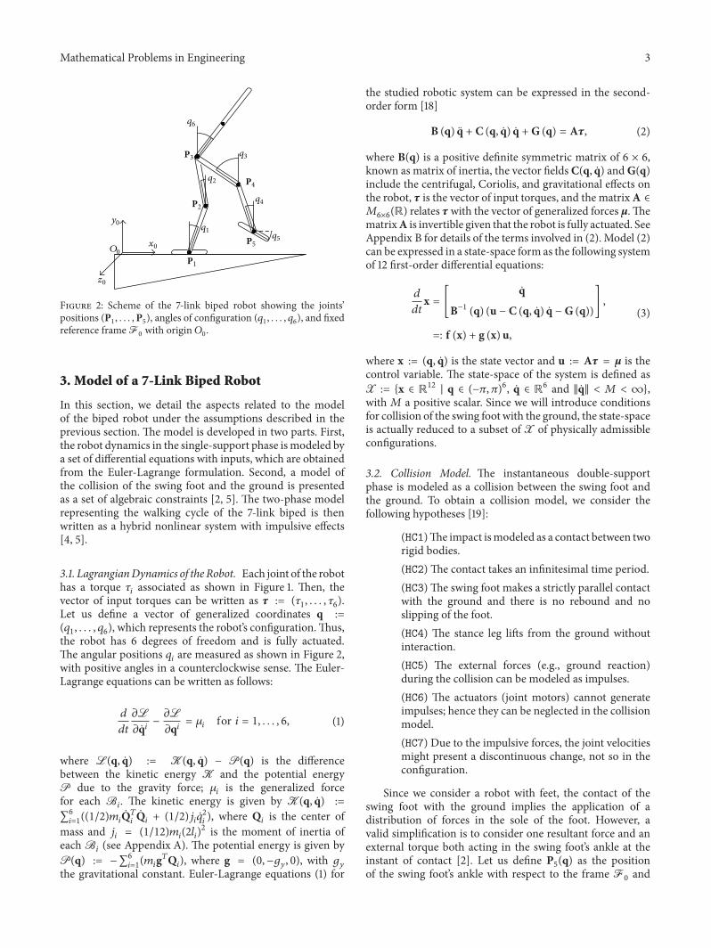
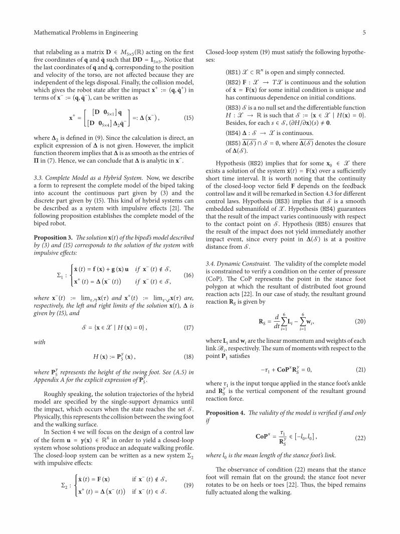
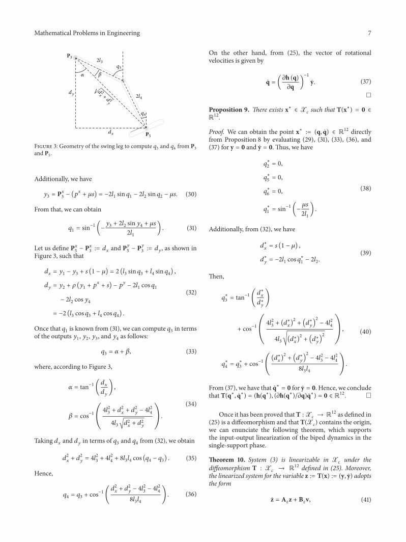
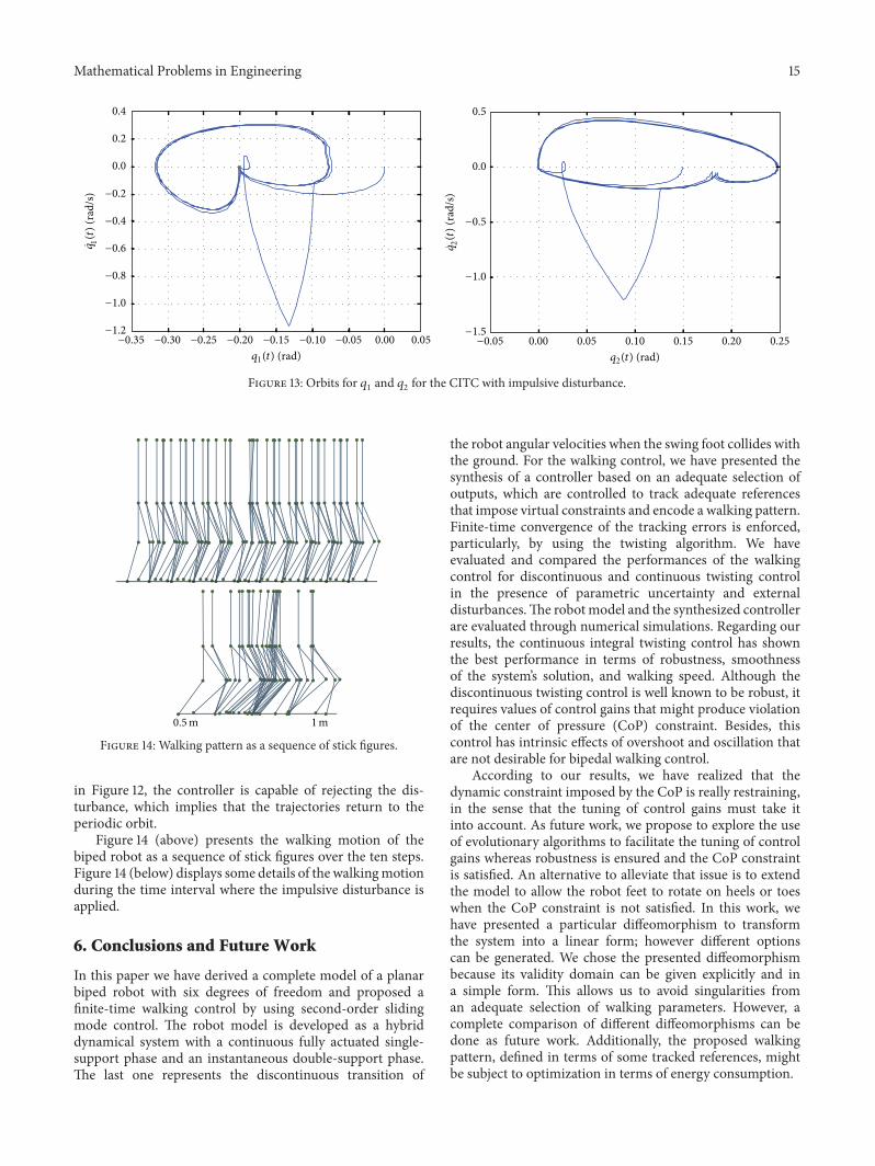