research article assessing the added value of...

Research ArticleAssessing the Added Value of Dynamical DownscalingUsing the Standardized Precipitation Index

Jared H. Bowden,1 Kevin D. Talgo,1 Tanya L. Spero,2 and Christopher G. Nolte2

1 Institute for the Environment, University of North Carolina at Chapel Hill, 100 Europa Drive, Campus Box 1105 (27599-1105),Chapel Hill, NC 27517, USA2Atmospheric Modeling and Analysis Division, National Exposure Research Laboratory,United States Environmental Protection Agency, 109 TW Alexander Drive, Research Triangle Park, NC 27711, USA

Correspondence should be addressed to Jared H. Bowden; [email protected]

Received 6 April 2015; Accepted 11 August 2015

Academic Editor: Eduardo Garcıa-Ortega

Copyright © 2016 Jared H. Bowden et al. This is an open access article distributed under the Creative Commons AttributionLicense, which permits unrestricted use, distribution, and reproduction in any medium, provided the original work is properlycited.

In this study, the Standardized Precipitation Index (SPI) is used to ascertain the added value of dynamical downscaling overthe contiguous United States. WRF is used as a regional climate model (RCM) to dynamically downscale reanalysis fields tocompare values of SPI over drought timescales that have implications for agriculture and water resources planning. The regionalclimate generated by WRF has the largest improvement over reanalysis for SPI correlation with observations as the droughttimescale increases.This suggests that dynamically downscaled fieldsmay bemore reliable than larger-scale fields for water resourceapplications (e.g., water storage within reservoirs). WRF improves the timing and intensity of moderate to extreme wet and dryperiods, even in regions with homogenous terrain. This study also examines changes in SPI from the extreme drought of 1988 andthree “drought busting” tropical storms. Each of those events illustrates the importance of using downscaling to resolve the spatialextent of droughts. The analysis of the “drought busting” tropical storms demonstrates that while the impact of these storms onending prolonged droughts is improved by the RCM relative to the reanalysis, it remains underestimated. These results illustratethe importance and some limitations of using RCMs to project drought.

1. Introduction

Drought impacts more people than any other natural disasterand is themost costly of all natural disasters with an estimated$6–$8 billion in global damage annually [1, 2]. Historicalrecords suggest increasingly severe and widespread droughtshave occurred over recent decades, a trend that is projectedto persist through the 21st century [3]. Global climate models(GCMs) are critical tools for drought projection because theycan simulate the large-scale atmospheric circulation responseto changes in radiative forcing. However, the coarse resolu-tion of most GCMs may limit the ability to project regionaldroughts. Regional climatemodels (RCMs) are typically usedto downscale GCM fields and this dynamically downscaledoutput may be an important resource for projecting changesin regional droughts. Many coordinated international effortswith RCMs are underway (e.g., CORDEX [4]) or completed

(e.g., NARCCAP [5], PRUDENCE [6], and ENSEMBLES [7])to represent the regional climatology at higher resolution. Forinstance, using a RCMcan improve the representation of landuse and land cover [8] and resolve mesoscale circulations andfeedbacks [9–11].

Droughts are commonly associated with large-scale shiftsin the atmospheric circulation and/or sea surface temperatureanomalies [12–14]. These large-scale features are resolved byGCMs, which have projected changes such as the polewardshift in the Hadley cell [15] or the westward migration ofthe Bermuda High [16]. Therefore, RCMs, which are forcedby GCM fields, may be limited in their ability to improvethe characterization of widespread droughts because suchdroughts are driven by the large-scale atmospheric circu-lation resolved by GCMs. In addition, RCMs typically useclimatological albedo values that can limit the land-surface-atmosphere feedbacks that affect drought [17]. However,

Hindawi Publishing CorporationAdvances in MeteorologyVolume 2016, Article ID 8432064, 14 pageshttp://dx.doi.org/10.1155/2016/8432064

2 Advances in Meteorology

RCMs may add value beyond the driving GCM at regionalto local scales by improving the precipitation variability(i.e., extremes) that is important for describing the regionalclimate or ending long-term droughts. Maule et al. [18]evaluatedRCMswithin the ENSEMBLESproject over Europeusing the Standardized Precipitation Index (SPI) and PalmerDrought Severity Index for hindcast simulations.They foundthat RCMs in ENSEMBLES could capture observed droughtfeatures, but those RCMs performed poorly in complexterrain regions and often did not correctly simulate themagnitude of droughts. Russo et al. [19] also evaluatedRCMs within the ENSEMBLES project and found that anonstationary form of the SPI reveals robust changes inextreme dry and wet years/seasons in a future climate overEurope. Overall, because droughts are commonly associatedwith shifts in the large-scale atmospheric circulation andthere are limitations with many RCMs using climatologicalalbedo values, it is important to demonstrate the added valueof a RCM for a drought metric such as the SPI. To ourknowledge, this type of comparison has not been performedpreviously and complements prior studies such asMaule et al.[18] and Russo et al. [19].

The objective of this paper is to evaluate hindcast simu-lations of SPI using the Weather Research and Forecasting(WRF) model [20] for dynamical downscaling over the con-tiguous United States (CONUS) to quantify the value addedby downscaling. In particular, this study identifies the addedvalue of using dynamically downscaled fields to computeSPI for different accumulation periods and different extremeevents, including a major drought and “drought busting”tropical storms. Section 2 describes the WRF model setup,and Section 3 describes the SPI. Section 4 contains statisticalanalyses of SPI over the 18-year simulation. Section 5 exploreschanges in SPI during the 1988 North American droughtand after the passages of tropical cyclones during the 1990and 1999 Atlantic hurricane seasons that helped to alleviatedrought conditions within the eastern U.S. Discussion andconclusions are provided in Section 6.

2. WRF Model Setup

TheWRFmodel version 3.4.1 was run continuously from 1988to 2005 after a one-month spin-up using a 108–36-km, two-way nested domain covering North America (Figure 1). Theinput data are 2.5∘ × 2.5∘ fields from the National Centersfor Environmental Prediction-Department of Energy Atmo-spheric Model Intercomparison Project (AMIP-II) Reanal-ysis data [21], hereinafter, R2. R2 data can be consideredas perfect lateral boundary conditions, permitting directcomparison with observations, and they have a horizontalresolution that is comparable to many GCMs. WRF wasrun with a 34-layer configuration with a model top at50 hPa. The physics options follow those used in Otte et al.[22], except that the simulation here used the Kain-Fritschconvective parameterization [23]. The simulation employsanalysis nudging on both domains with nudging coefficientsfollowingOtte et al. [22]. Analysis nudging has been shown toimprove the large-scale atmospheric circulation within WRF[24] as well as the mean and extreme 2-m temperature and

40∘N

30∘N

20∘N

10∘N

120∘W 105

∘W 90∘W 75

∘W

d02

Figure 1:WRF 108-km and 36-km (“d02”) domains. Shaded regionsare the NCDC climate regions.

precipitation [22, 24, 25] in regional climate modeling forcedby historical data.

3. Standardized Precipitation Index

This study uses the SPI [26, 27] to identifywet and dry periodsand classify their severity within the 18-year simulationperiod. The SPI is appealing since it is based solely onprecipitation, which is readily available from RCMs; otherdrought indices rely on fields that often need to be derivedor inferred from RCM output. The SPI can be applied acrossmany short-term climatic timescales and is equally effectivein categorizing wet and dry periods.

To calculate SPI, the long-term monthly precipitationrecord is fitted to a gamma distribution which is thentransformed into a normal distribution so that the meanSPI at each location and over the desired period is zero[28]. The SPI value for the total precipitation over someperiod (of specific months and of a certain duration) is thenumber of standard deviations from the climatological meanfor the same relative period and timescale. For example,a 3-month SPI at the end of August compares the June–August precipitation total in that particular year with theJune–August precipitation totals of all the years on record forthat location. Positive SPI values indicate higher than meanprecipitation, and negative values indicate lower than meanprecipitation. Absolute values of SPI ranging from 1.00 to 1.49are considered to be moderate events. Absolute values of SPIbetween 1.50 and 1.99 are classified as severe events. Extremeevents, defined as having an absolute value of SPI greater than2, occur only 2.3% of the time [18].

The SPI can be calculated over different accumulationperiods (i.e., timescales) ranging from one month up to 72months. Changing the accumulation period in the SPI canbe used to differentiate between various types of droughtconditions. SPI timescales in the 1- to 3-month range can beused for applications that respond to short-term precipitationanomalies, such as meteorological drought, soil moistureretention, and agriculture. SPI timescales in the 6- to 12-month range can be used to assess impacts to groundwater,streamflow, and reservoir levels.

Advances in Meteorology 3

1-m

onth

SPI

West

1988 1990 1992 1994 1996 1998 2000 2002 2004

1988 1990 1992 1994 1996 1998 2000 2002 2004

1988 1990 1992 1994 1996 1998 2000 2002 2004

1-m

onth

SPI

Northern Rockies and Plains

1-m

onth

SPI

Southeast

2

1

0

−1

−2

2

1

0

−1

−2

2

1

0

−1

−2

1940–20061988–2006

(a)

1988 1990 1992 1994 1996 1998 2000 2002 2004

1988 1990 1992 1994 1996 1998 2000 2002 2004

1988 1990 1992 1994 1996 1998 2000 2002 2004

West

Northern Rockies and Plains

Southeast

12-m

onth

SPI

12

-mon

th S

PI12

-mon

th S

PI 2

1

0

−1

−2

2

1

0

−1

−2

2

1

0

−1

−2

1940–20061988–2006

(b)

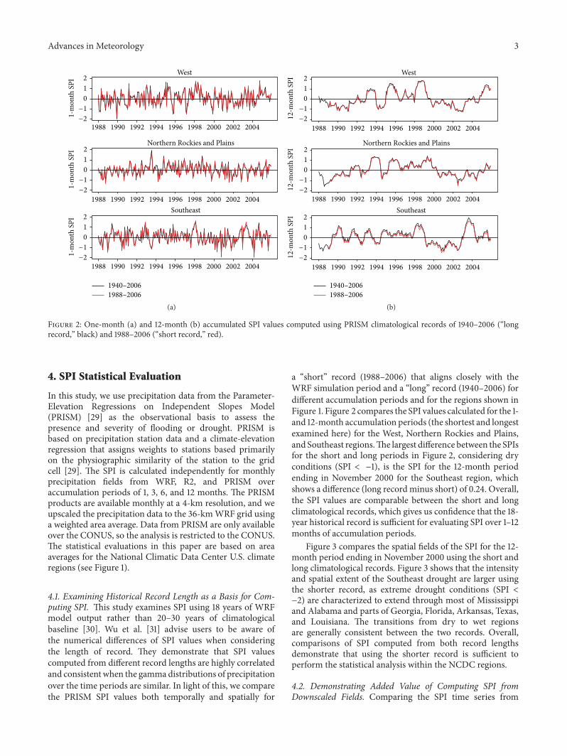
Figure 2: One-month (a) and 12-month (b) accumulated SPI values computed using PRISM climatological records of 1940–2006 (“longrecord,” black) and 1988–2006 (“short record,” red).

4. SPI Statistical Evaluation

In this study, we use precipitation data from the Parameter-Elevation Regressions on Independent Slopes Model(PRISM) [29] as the observational basis to assess thepresence and severity of flooding or drought. PRISM isbased on precipitation station data and a climate-elevationregression that assigns weights to stations based primarilyon the physiographic similarity of the station to the gridcell [29]. The SPI is calculated independently for monthlyprecipitation fields from WRF, R2, and PRISM overaccumulation periods of 1, 3, 6, and 12 months. The PRISMproducts are available monthly at a 4-km resolution, and weupscaled the precipitation data to the 36-kmWRF grid usinga weighted area average. Data from PRISM are only availableover the CONUS, so the analysis is restricted to the CONUS.The statistical evaluations in this paper are based on areaaverages for the National Climatic Data Center U.S. climateregions (see Figure 1).

4.1. Examining Historical Record Length as a Basis for Com-puting SPI. This study examines SPI using 18 years of WRFmodel output rather than 20–30 years of climatologicalbaseline [30]. Wu et al. [31] advise users to be aware ofthe numerical differences of SPI values when consideringthe length of record. They demonstrate that SPI valuescomputed from different record lengths are highly correlatedand consistent when the gammadistributions of precipitationover the time periods are similar. In light of this, we comparethe PRISM SPI values both temporally and spatially for

a “short” record (1988–2006) that aligns closely with theWRF simulation period and a “long” record (1940–2006) fordifferent accumulation periods and for the regions shown inFigure 1. Figure 2 compares the SPI values calculated for the 1-and 12-month accumulation periods (the shortest and longestexamined here) for the West, Northern Rockies and Plains,and Southeast regions.The largest difference between the SPIsfor the short and long periods in Figure 2, considering dryconditions (SPI < −1), is the SPI for the 12-month periodending in November 2000 for the Southeast region, whichshows a difference (long recordminus short) of 0.24. Overall,the SPI values are comparable between the short and longclimatological records, which gives us confidence that the 18-year historical record is sufficient for evaluating SPI over 1–12months of accumulation periods.

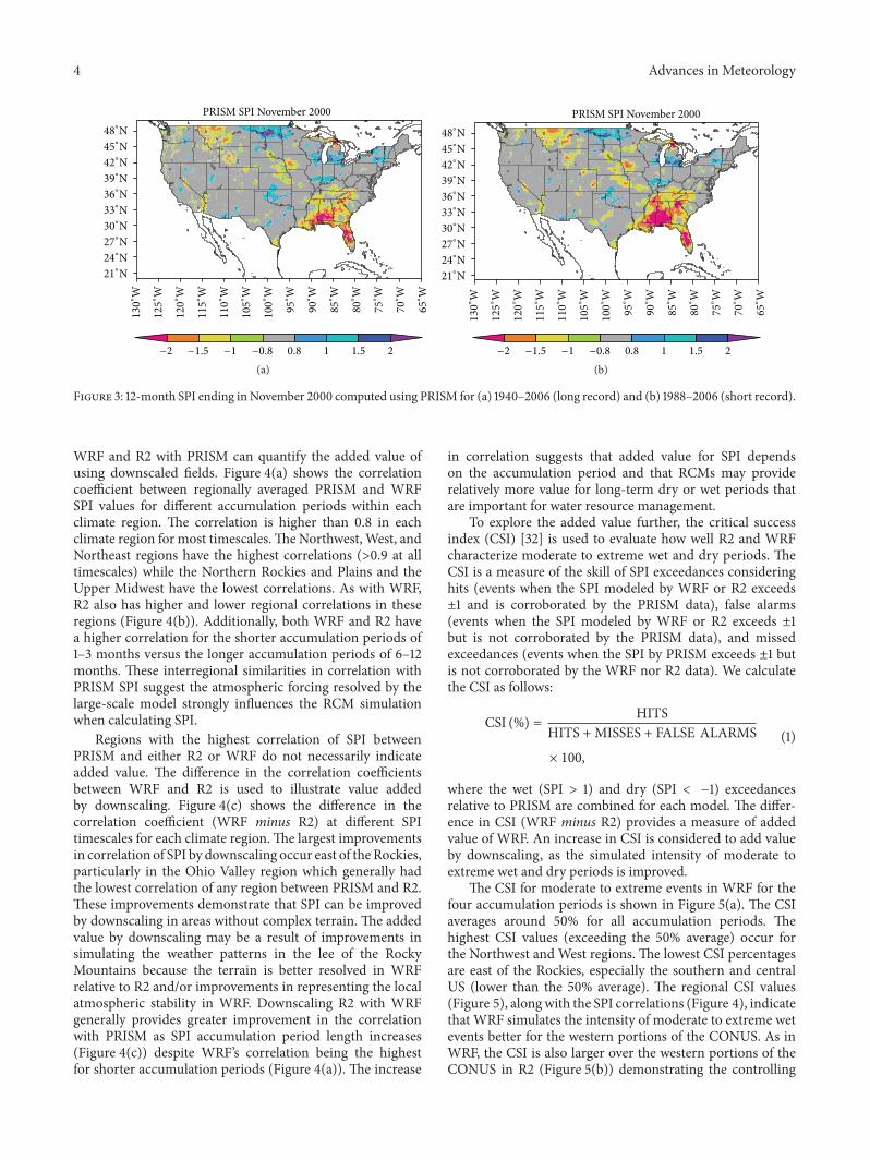
Figure 3 compares the spatial fields of the SPI for the 12-month period ending in November 2000 using the short andlong climatological records. Figure 3 shows that the intensityand spatial extent of the Southeast drought are larger usingthe shorter record, as extreme drought conditions (SPI <−2) are characterized to extend through most of Mississippiand Alabama and parts of Georgia, Florida, Arkansas, Texas,and Louisiana. The transitions from dry to wet regionsare generally consistent between the two records. Overall,comparisons of SPI computed from both record lengthsdemonstrate that using the shorter record is sufficient toperform the statistical analysis within the NCDC regions.

4.2. Demonstrating Added Value of Computing SPI fromDownscaled Fields. Comparing the SPI time series from


48∘N

45∘N

42∘N

39∘N

36∘N

33∘N

30∘N

27∘N

24∘N

21∘N

130∘W

125∘W

120∘W

115∘W

110∘W

105∘W

100∘W

95∘W

90∘W

85∘W

80∘W

75∘W

70∘W

65∘W

PRISM SPI November 2000

−2 −1.5 −1 −0.8 0.8 1 1.5 2

(a)

48∘N

45∘N

42∘N

39∘N

36∘N

33∘N

30∘N

27∘N

24∘N

21∘N

130∘W

125∘W

120∘W

115∘W

110∘W

105∘W

100∘W

95∘W

90∘W

85∘W

80∘W

75∘W

70∘W

65∘W

PRISM SPI November 2000

−2 −1.5 −1 −0.8 0.8 1 1.5 2

(b)

Figure 3: 12-month SPI ending in November 2000 computed using PRISM for (a) 1940–2006 (long record) and (b) 1988–2006 (short record).

WRF and R2 with PRISM can quantify the added value ofusing downscaled fields. Figure 4(a) shows the correlationcoefficient between regionally averaged PRISM and WRFSPI values for different accumulation periods within eachclimate region. The correlation is higher than 0.8 in eachclimate region for most timescales.TheNorthwest, West, andNortheast regions have the highest correlations (>0.9 at alltimescales) while the Northern Rockies and Plains and theUpper Midwest have the lowest correlations. As with WRF,R2 also has higher and lower regional correlations in theseregions (Figure 4(b)). Additionally, both WRF and R2 havea higher correlation for the shorter accumulation periods of1–3 months versus the longer accumulation periods of 6–12months. These interregional similarities in correlation withPRISM SPI suggest the atmospheric forcing resolved by thelarge-scale model strongly influences the RCM simulationwhen calculating SPI.

Regions with the highest correlation of SPI betweenPRISM and either R2 or WRF do not necessarily indicateadded value. The difference in the correlation coefficientsbetween WRF and R2 is used to illustrate value addedby downscaling. Figure 4(c) shows the difference in thecorrelation coefficient (WRF minus R2) at different SPItimescales for each climate region.The largest improvementsin correlation of SPI by downscaling occur east of theRockies,particularly in the Ohio Valley region which generally hadthe lowest correlation of any region between PRISM and R2.These improvements demonstrate that SPI can be improvedby downscaling in areas without complex terrain. The addedvalue by downscaling may be a result of improvements insimulating the weather patterns in the lee of the RockyMountains because the terrain is better resolved in WRFrelative to R2 and/or improvements in representing the localatmospheric stability in WRF. Downscaling R2 with WRFgenerally provides greater improvement in the correlationwith PRISM as SPI accumulation period length increases(Figure 4(c)) despite WRF’s correlation being the highestfor shorter accumulation periods (Figure 4(a)). The increase

in correlation suggests that added value for SPI dependson the accumulation period and that RCMs may providerelatively more value for long-term dry or wet periods thatare important for water resource management.

To explore the added value further, the critical successindex (CSI) [32] is used to evaluate how well R2 and WRFcharacterize moderate to extreme wet and dry periods. TheCSI is a measure of the skill of SPI exceedances consideringhits (events when the SPI modeled by WRF or R2 exceeds±1 and is corroborated by the PRISM data), false alarms(events when the SPI modeled by WRF or R2 exceeds ±1but is not corroborated by the PRISM data), and missedexceedances (events when the SPI by PRISM exceeds ±1 butis not corroborated by the WRF nor R2 data). We calculatethe CSI as follows:

CSI (%) = HITSHITS +MISSES + FALSE ALARMS

× 100,

(1)

where the wet (SPI > 1) and dry (SPI < −1) exceedancesrelative to PRISM are combined for each model. The differ-ence in CSI (WRF minus R2) provides a measure of addedvalue of WRF. An increase in CSI is considered to add valueby downscaling, as the simulated intensity of moderate toextreme wet and dry periods is improved.

The CSI for moderate to extreme events in WRF for thefour accumulation periods is shown in Figure 5(a). The CSIaverages around 50% for all accumulation periods. Thehighest CSI values (exceeding the 50% average) occur forthe Northwest and West regions. The lowest CSI percentagesare east of the Rockies, especially the southern and centralUS (lower than the 50% average). The regional CSI values(Figure 5), alongwith the SPI correlations (Figure 4), indicatethat WRF simulates the intensity of moderate to extreme wetevents better for the western portions of the CONUS. As inWRF, the CSI is also larger over the western portions of theCONUS in R2 (Figure 5(b)) demonstrating the controlling


0

0.1

0.2

0.3

0.4

0.5

0.6

0.7

0.8

0.9

1

Cor

rela

tion

WRF correlation

1 month3 months

6 months12 months

Nor

thw

est

Wes

t

Nor

ther

n Ro

ckie

san

d Pl

ains

Sout

hwes

t

Upp

erM

idw

est

Sout

h

Ohi

oVa

lley

Sout

heas

t

Nor

thea

st

Aver

age

(a)

0

0.1

0.2

0.3

0.4

0.5

0.6

0.7

0.8

0.9

1

Cor

relat

ion

1 month3 months

6 months12 months

R2 correlation

Nor

thw

est

Wes

t

Nor

ther

n Ro

ckie

san

d Pl

ains

Sout

hwes

t

Upp

erM

idw

est

Sout

h

Ohi

oVa

lley

Sout

heas

t

Nor

thea

st

Aver

age

(b)

Nor

thw

est

Wes

t

Nor

ther

n Ro

ckie

san

d Pl

ains

Sout

hwes

t

Upp

erM

idw

est

Sout

h

Ohi

oVa

lley

Sout

heas

t

Nor

thea

st

Aver

age

1 month3 months

6 months12 months

−0.05

0

0.05

0.1

0.15

0.2

0.25

Cor

relat

ion

diffe

renc

e

WRF minus R2 correlation

(c)

Figure 4: SPI correlation coefficient between (a) WRF and PRISM and (b) R2 and PRISM for 1-, 3-, 6-, and 12-month accumulation periodsaveraged over each NCDC climate region. (c) Difference betweenWRF and R2 correlation coefficient (WRFminus R2) for the same periodsand regions as in (a) and (b).

influence of the large-scale atmospheric forcing for SPIvalues.

Figure 5(c) compares the CSIs for moderate to extremeexceedances from WRF and R2. In general, the CSI is largerinWRF for the majority of the CONUS, which demonstratesthere is added value by dynamical downscaling. Acrossthe regions and accumulation periods, there are severalinstances of the CSI for wet and dry events increasing with

WRF by more than 15% compared to R2. In particular, theNortheast region has the largest overall improvement in CSIby downscaling, especially for longer accumulation periods.On average, across theCONUS,WRFprovidesmore value forlonger accumulation periods, though overall CSI improvesby 5–10% for each accumulation period. While projectionsof moderate to extreme dry and wet periods are improvedby downscaling, added value for these events is spatially


0

10

20

30

40

50

60

70

80

90

100WRF CSI wet and dry exceedances

Criti

cal s

ucce

ss in

dex

(%)

1 month3 months

6 months12 months

Nor

thw

est

Wes

t

Nor

ther

n Ro

ckie

san

d Pl

ains

Sout

hwes

t

Upp

erM

idw

est

Sout

h

Ohi

oVa

lley

Sout

heas

t

Nor

thea

st

Aver

age

(a)

0

10

20

30

40

50

60

70

80

90

100R2 CSI wet and dry exceedances

Criti

cal s

ucce

ss in

dex

(%)

1 month3 months

6 months12 months

Nor

thw

est

Wes

t

Nor

ther

n Ro

ckie

san

d Pl

ains

Sout

hwes

t

Upp

erM

idw

est

Sout

h

Ohi

oVa

lley

Sout

heas

t

Nor

thea

st

Aver

age

(b)

−15

−10

−5

0

5

10

15

20

25

30

35

Criti

cal s

ucce

ss in

dex

diffe

renc

e (%

)

WRF minus R2 CSI wet and dry exceedances

1 month3 months

6 months12 months

Nor

thw

est

Wes

t

Nor

ther

n Ro

ckie

san

d Pl

ains

Sout

hwes

t

Upp

erM

idw

est

Sout

h

Ohi

oVa

lley

Sout

heas

t

Nor

thea

st

Aver

age

(c)Figure 5: CSI for |SPI| > 1 between (a) WRF and PRISM and (b) R2 and PRISM for 1-, 3-, 6-, and 12-month accumulation periods averagedover each NCDC climate region. (c) Difference between WRF and R2 CSI (WRF minus R2) for the same periods and regions as in (a) and(b).

inconsistent which indicates the complexity of assessingadded value using a RCM for moderate to extreme dry or wetperiods. For instance, the added value in the Northeast fromdownscaling may result from improvements in simulatingthe mesoscale circulation and precipitation when using aRCM, such as latent heating in midlatitude cyclones [11]. Bycontrast, smaller improvements over the western U.S. suggestthat the large-scale atmospheric circulation in R2 (which

was retained in WRF through the lateral boundaries and bynudging) sufficiently resolves droughts and floods in thoseregions.

5. SPI Event Analysis

Examining the SPI during significant meteorological eventscan provide further insight into added value by downscaling


48∘N

45∘N

42∘N

39∘N

36∘N

33∘N

30∘N

27∘N

24∘N

21∘N

130∘W

125∘W

120∘W

115∘W

110∘W

105∘W

100∘W

95∘W

90∘W

85∘W

80∘W

75∘W

70∘W

65∘W

−2 −1.5 −1 −0.8 0.8 1 1.5 2

PRISM SPI December 1988

(a)

48∘N

45∘N

42∘N

39∘N

36∘N

33∘N

30∘N

27∘N

24∘N

21∘N

130∘W

125∘W

120∘W

115∘W

110∘W

105∘W

100∘W

95∘W

90∘W

85∘W

80∘W

75∘W

70∘W

65∘W

−2 −1.5 −1 −0.8 0.8 1 1.5 2

R2 SPI December 1988

(b)

48∘N

45∘N

42∘N

39∘N

36∘N

33∘N

30∘N

27∘N

24∘N

21∘N

130∘W

125∘W

120∘W

115∘W

110∘W

105∘W

100∘W

95∘W

90∘W

85∘W

80∘W

75∘W

70∘W

65∘W

−2 −1.5 −1 −0.8 0.8 1 1.5 2

WRF SPI December 1988

(c)

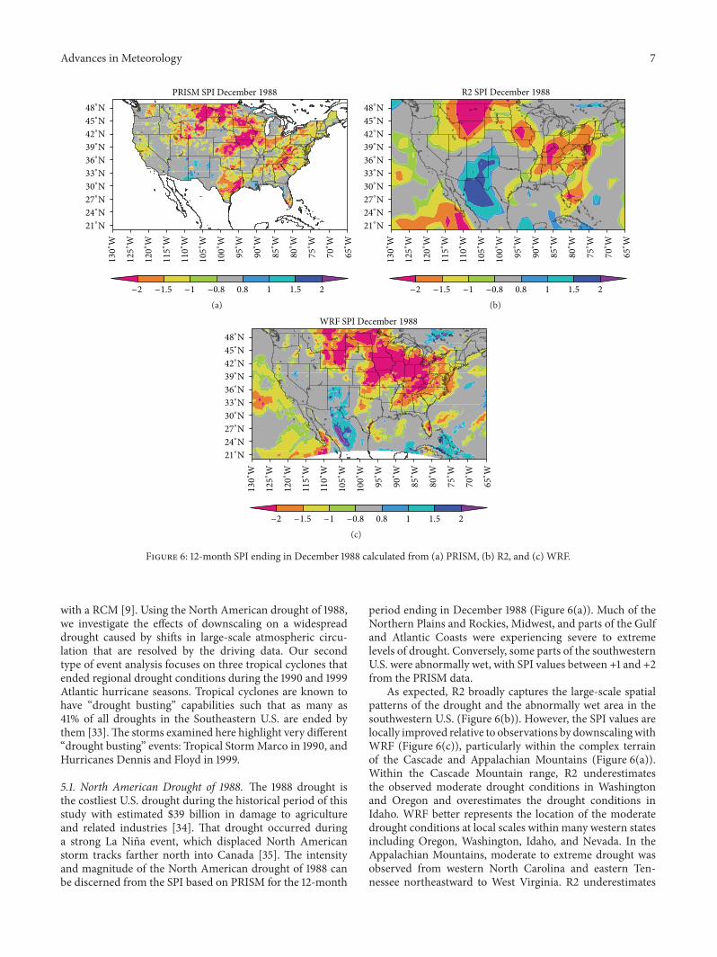
Figure 6: 12-month SPI ending in December 1988 calculated from (a) PRISM, (b) R2, and (c) WRF.

with a RCM [9]. Using the North American drought of 1988,we investigate the effects of downscaling on a widespreaddrought caused by shifts in large-scale atmospheric circu-lation that are resolved by the driving data. Our secondtype of event analysis focuses on three tropical cyclones thatended regional drought conditions during the 1990 and 1999Atlantic hurricane seasons. Tropical cyclones are known tohave “drought busting” capabilities such that as many as41% of all droughts in the Southeastern U.S. are ended bythem [33].The storms examined here highlight very different“drought busting” events: Tropical StormMarco in 1990, andHurricanes Dennis and Floyd in 1999.

5.1. North American Drought of 1988. The 1988 drought isthe costliest U.S. drought during the historical period of thisstudy with estimated $39 billion in damage to agricultureand related industries [34]. That drought occurred duringa strong La Nina event, which displaced North Americanstorm tracks farther north into Canada [35]. The intensityand magnitude of the North American drought of 1988 canbe discerned from the SPI based on PRISM for the 12-month

period ending in December 1988 (Figure 6(a)). Much of theNorthern Plains and Rockies, Midwest, and parts of the Gulfand Atlantic Coasts were experiencing severe to extremelevels of drought. Conversely, some parts of the southwesternU.S. were abnormally wet, with SPI values between +1 and +2from the PRISM data.

As expected, R2 broadly captures the large-scale spatialpatterns of the drought and the abnormally wet area in thesouthwestern U.S. (Figure 6(b)). However, the SPI values arelocally improved relative to observations by downscalingwithWRF (Figure 6(c)), particularly within the complex terrainof the Cascade and Appalachian Mountains (Figure 6(a)).Within the Cascade Mountain range, R2 underestimatesthe observed moderate drought conditions in Washingtonand Oregon and overestimates the drought conditions inIdaho. WRF better represents the location of the moderatedrought conditions at local scales within many western statesincluding Oregon, Washington, Idaho, and Nevada. In theAppalachian Mountains, moderate to extreme drought wasobserved from western North Carolina and eastern Ten-nessee northeastward to West Virginia. R2 underestimates


the severity of the drought for these locations, while WRFimproves representation of the intensity and placement ofthe drought. Some of the largest differences occur in Kansasand Oklahoma, an area with fairly uniform terrain andextensive agriculture and ranching.The horizontal resolutionof R2 cannot resolve the gradient between wetter conditionsin the Southwest and drought in the Great Plains. WRFcaptures the intensity and location of the drought withinKansas and Oklahoma while also improving the placementand magnitude of the wetter conditions in the Southwest.The SPI computed from WRF also has some shortcomings:notably, the overpredicted intensity of the drought in theUpper Midwest and Ohio Valley and the miss of the droughtalong the Texas coast. Overall, this example illustrates thatdownscaling can add value at local scales when using SPI tocharacterize the spatial extent of droughts.

5.2. 1990 Tropical Storm Marco. Tropical Storm Marcodumped locally heavy amounts of rainfall between October10 and October 13, 1990, across parts of the Southeast U.S.,exceeding 10 inches in many locations throughout Georgia,South Carolina, and North Carolina [33, 36]. The heavyrainfall and associated flooding caused $57million in damageand was responsible for 7 deaths [37]. Tropical Storm Marcowas noteworthy because of its role in the formation andevolution of two mesoscale features (cold-air damming andcoastal frontogenesis) over Georgia and the Carolinas thatenhanced the local precipitation over these areas on October10 and October 11. These mesoscale features formed whileTropical StormMarcowas centered over southern and centralFlorida more than 400 km away [33, 36]. Prior to TropicalStormMarco, Southeastern Atlantic states were experiencingdrought conditions [33]. Below we compare the SPI valuesbefore and after Tropical Storm Marco to evaluate the addedvalue of WRF for a “drought busting” tropical cyclone thatinduces mesoscale features important for rainfall totals.

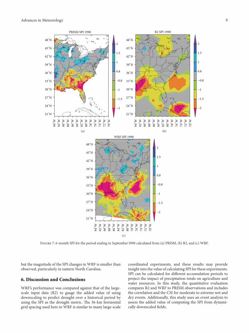
Figure 7(a) illustrates the observed drought using the 6-month SPI calculated from PRISM prior to the landfall ofTropical StormMarco inOctober 1990.The SPI values are lessthan −2 (extreme drought) in many locations throughout theSoutheast. Figures 7(b) and 7(c) show the 6-month SPI valuesfrom R2 and WRF for the same period. The drought usingR2 is farther west and misses the drought that extends fromGeorgia into South andNorthCarolina. In comparison,WRFis able to capture drier conditions over Georgia extendinginto South Carolina, but the magnitude of the drought is lessintense than observed. Note that the most intense drought inWRF, with SPI values less than −2, follows the general patternreflected in R2 with the driest conditions farther west intoLouisiana and Mississippi.

After Tropical Storm Marco made landfall, the extremedrought in southern Georgia was alleviated (compare Fig-ures 7(a) and 8(a)). Additionally, there is a reversal in theSPI towards wetter than average conditions in central andwestern portions of North and South Carolina. AlthoughWRF underestimated the intensity of the drought, especiallyfor Southeastern Georgia (compare Figures 7(a) and 7(c)),it captures the relative shift towards neutral conditions.However, the reversal in the SPI values in WRF and R2 is

similar for the Southeastern Atlantic states and neither has astrong reversal in the SPI values as observed. Comparing theSPIs fromR2 andWRF indicates thatWRFprovides relativelysmall value in this case despite Tropical Storm Marco’s rolein the formation of mesoscale features that led to copiousamounts of rainfall.

5.3. 1999 Hurricanes Dennis and Floyd. The 1999 Atlantichurricane season includedHurricane Floyd, which generatedthe costliest flooding event in North Carolina history with anestimated total cost exceeding $9 billion [34]. The back-to-back combination ofHurricanesDennis andFloyd inAugust-September 1999 altered the regional and local drought signalsin parts of the eastern seaboard of theU.S. as the region transi-tioned out of a period of prolonged drought. In particular, thetracks of Dennis and Floyd crossed eastern North Carolinaless than two weeks apart, resulting in historic flooding ofthe Tar River and inundation of the town of Princeville[38]. The localized heavy rainfall, especially over easternNorth Carolina, provides another ideal event to investigatethe added value of increasing the horizontal resolution forsimulating “drought busting” tropical cyclones.

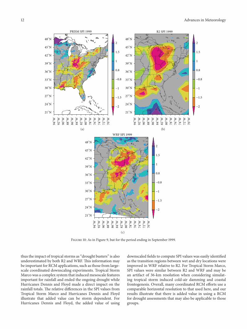
Prior to Hurricanes Dennis and Floyd in 1999, much ofthe Mid-Atlantic and Northeast was experiencing a long-term moderate to extreme drought, as evident in the 12-month SPI calculated from PRISM and ending in July 1999(Figure 9(a)), particularly seen from North Carolina intothe Mid-Atlantic states with SPI values less than −1. Thepassages of Hurricanes Dennis and Floyd in late Augustand early September, 1999, respectively, brought relief todrought-stricken areas along the Atlantic coast.Those stormsshifted the moderate-extreme drought in July 1999 to nearlyneutral conditions for most locations east of the AppalachianMountains after the storms, as seen by comparing the 12-month SPI ending in July 1999 (Figure 9(a)) to that ending inSeptember 1999 (Figure 10(a)). Eastern North Carolina andSoutheastern Virginia experienced historic flooding duringthis time, and the precipitation received from these stormsover this short period completely reversed the 12-month SPIto abnormally wet conditions, as reflected in the local SPIvalues above +2 in some areas (Figure 10(a)). Portions of theOhio Valley states, which did not receive precipitation fromthose storms (not shown), remained in extreme drought.

WRF provides a better estimate of the drought for the 12-month SPI ending in July 1999 than R2 prior to HurricanesDennis and Floyd, especially for the Northeastern states(see Figures 9(b) and 9(c)). For instance, WRF correctlyidentified the drought extending into Northern New York,Vermont, and New Hampshire, but it was absent in R2.Figure 9 clearly shows that the coarser horizontal resolutionin R2 limits the ability to capture transition regions of wet anddry conditions, as in Northern New York. Figure 10 showsthat, after the passages of Hurricanes Dennis and Floyd, bothR2 and WRF captured the relief of the long-term droughtconditions for locations east of the Appalachian Mountains,especially notable in North Carolina and Virginia. WRFimproves the spatial gradient of the SPI values relative to R2,


48∘N

45∘N

42∘N

39∘N

36∘N

33∘N

30∘N

27∘N

24∘N

21∘N

94∘W

92∘W

90∘W

88∘W

86∘W

84∘W

82∘W

80∘W

78∘W

76∘W

74∘W

72∘W

70∘W

−2

−1.5

−1

−0.8

0.8

1

1.5

2

PRISM SPI 1990

(a)

48∘N

45∘N

42∘N

39∘N

36∘N

33∘N

30∘N

27∘N

24∘N

21∘N

94∘W

92∘W

90∘W

88∘W

86∘W

84∘W

82∘W

80∘W

78∘W

76∘W

74∘W

72∘W

70∘W

−2

−1.5

−1

−0.8

0.8

1

1.5

2

R2 SPI 1990

(b)

48∘N

45∘N

42∘N

39∘N

36∘N

33∘N

30∘N

27∘N

24∘N

21∘N

94∘W

92∘W

90∘W

88∘W

86∘W

84∘W

82∘W

80∘W

78∘W

76∘W

74∘W

72∘W

70∘W

−2

−1.5

−1

−0.8

0.8

1

1.5

2

WRF SPI 1990

(c)

Figure 7: 6-month SPI for the period ending in September 1990 calculated from (a) PRISM, (b) R2, and (c) WRF.

but the magnitude of the SPI changes inWRF is smaller thanobserved, particularly in eastern North Carolina.

6. Discussion and Conclusions

WRF’s performance was compared against that of the large-scale input data (R2) to gauge the added value of usingdownscaling to predict drought over a historical period byusing the SPI as the drought metric. The 36-km horizontalgrid spacing used here in WRF is similar to many large-scale

coordinated experiments, and these results may provideinsight into the value of calculating SPI for these experiments.SPI can be calculated for different accumulation periods toproject the impact of precipitation totals on agriculture andwater resources. In this study, the quantitative evaluationcompares R2 and WRF to PRISM observations and includesthe correlation and the CSI for moderate to extreme wet anddry events. Additionally, this study uses an event analysis toassess the added value of computing the SPI from dynami-cally downscaled fields.


48∘N

45∘N

42∘N

39∘N

36∘N

33∘N

30∘N

27∘N

24∘N

21∘N

94∘W

92∘W

90∘W

88∘W

86∘W

84∘W

82∘W

80∘W

78∘W

76∘W

74∘W

72∘W

70∘W

−2

−1.5

−1

−0.8

0.8

1

1.5

2

PRISM SPI 1990

(a)

48∘N

45∘N

42∘N

39∘N

36∘N

33∘N

30∘N

27∘N

24∘N

21∘N

94∘W

92∘W

90∘W

88∘W

86∘W

84∘W

82∘W

80∘W

78∘W

76∘W

74∘W

72∘W

70∘W

−2

−1.5

−1

−0.8

0.8

1

1.5

2

R2 SPI 1990

(b)

48∘N

45∘N

42∘N

39∘N

36∘N

33∘N

30∘N

27∘N

24∘N

21∘N

94∘W

92∘W

90∘W

88∘W

86∘W

84∘W

82∘W

80∘W

78∘W

76∘W

74∘W

72∘W

70∘W

−2

−1.5

−1

−0.8

0.8

1

1.5

2

WRF SPI 1990

(c)

Figure 8: As in Figure 7, but for the period ending in October 1990.

The SPI correlation with observations decreases forlonger accumulation periods in both R2 and WRF anddemonstrates the influence of the large-scale atmosphericforcing on the SPI values. In general, SPI values in WRFfollow R2 as expected, but WRF also provides added value atthe NCDC regional scales.The largest added value occurs forlonger accumulation periods. The implication of this resultis that water resource applications (e.g., water storage withinreservoirs) may benefit more when using dynamically down-scaled precipitation. The regional scale statistics, including

the CSI calculation for moderate to extreme dry and wetevents, also reveal that WRF adds value for extreme/wet dryevents and in areas without complex terrain.The results indi-cate that downscaling is particularly beneficial to categorizethe intensity of moderate to extreme wet and dry periods,especially within NCDC regions east of the Rockies.

Because averaging SPI values over large regions cansometimes mask the local variations within a NCDC cli-mate region, particularly when a region includes areaswith SPI values of the opposite sign, we examined SPI


48∘N

45∘N

42∘N

39∘N

36∘N

33∘N

30∘N

27∘N

24∘N

21∘N

94∘W

92∘W

90∘W

88∘W

86∘W

84∘W

82∘W

80∘W

78∘W

76∘W

74∘W

72∘W

70∘W

−2

−1.5

−1

−0.8

0.8

1

1.5

2

PRISM SPI 1999

(a)

48∘N

45∘N

42∘N

39∘N

36∘N

33∘N

30∘N

27∘N

24∘N

21∘N

94∘W

92∘W

90∘W

88∘W

86∘W

84∘W

82∘W

80∘W

78∘W

76∘W

74∘W

72∘W

70∘W

−2

−1.5

−1

−0.8

0.8

1

1.5

2

R2 SPI 1999

(b)

48∘N

45∘N

42∘N

39∘N

36∘N

33∘N

30∘N

27∘N

24∘N

21∘N

94∘W

92∘W

90∘W

88∘W

86∘W

84∘W

82∘W

80∘W

78∘W

76∘W

74∘W

72∘W

70∘W

−2

−1.5

−1

−0.8

0.8

1

1.5

2

WRF SPI 1999

(c)

Figure 9: 12-month SPI for the period ending in July 1999 calculated from (a) PRISM, (b) R2, and (c) WRF.

predictions spatially using events with important local effects.For the 1988 North American drought, WRF improvedthe drought placement and magnitude within the NCDCregions. Many times added value is associated with better-resolved terrain, land use, and land/water boundaries. The1988 North American drought occurred in regions withoutcomplex terrain, such as the Great Plains. The Great Plainswas a transition region in R2 between extremely dry andwet areas, and the coarse resolution of R2 failed to capturesome areas of drought as large as the states of Kansas andOklahoma. By contrast, WRF better simulates the location

and intensity of the drought because it resolves the SPIgradient. The significance of this result is that large-scaledroughts, despite being generally associated with large-scaleatmospheric circulation shifts and resolvable by the drivingdata, are better resolved with dynamical downscaling in bothregions with and without complex terrain.

We also examined the added value of using a RCM for“drought busting” tropical cyclones. Tropical Storm Marco(1990) and Hurricanes Dennis and Floyd (1999) reveal thatthe reversal of SPI values to wet or near normal conditionsafter a prolonged drought is typically underestimated and


48∘N

45∘N

42∘N

39∘N

36∘N

33∘N

30∘N

27∘N

24∘N

21∘N

94∘W

92∘W

90∘W

88∘W

86∘W

84∘W

82∘W

80∘W

78∘W

76∘W

74∘W

72∘W

70∘W

−2

−1.5

−1

−0.8

0.8

1

1.5

2

PRISM SPI 1999

(a)

48∘N

45∘N

42∘N

39∘N

36∘N

33∘N

30∘N

27∘N

24∘N

21∘N

94∘W

92∘W

90∘W

88∘W

86∘W

84∘W

82∘W

80∘W

78∘W

76∘W

74∘W

72∘W

70∘W

−2

−1.5

−1

−0.8

0.8

1

1.5

2

R2 SPI 1999

(b)

48∘N

45∘N

42∘N

39∘N

36∘N

33∘N

30∘N

27∘N

24∘N

21∘N

94∘W

92∘W

90∘W

88∘W

86∘W

84∘W

82∘W

80∘W

78∘W

76∘W

74∘W

72∘W

70∘W

−2

−1.5

−1

−0.8

0.8

1

1.5

2

WRF SPI 1999

(c)

Figure 10: As in Figure 9, but for the period ending in September 1999.

thus the impact of tropical storms as “drought busters” is alsounderestimated by both R2 and WRF. This information maybe important for RCM applications, such as those from large-scale coordinated downscaling experiments. Tropical StormMarco was a complex system that inducedmesoscale featuresimportant for rainfall and ended the ongoing drought whileHurricanes Dennis and Floyd made a direct impact on therainfall totals. The relative differences in the SPI values fromTropical Storm Marco and Hurricanes Dennis and Floydillustrate that added value can be storm dependent. ForHurricanes Dennis and Floyd, the added value of using

downscaled fields to compute SPI values was easily identifiedas the transition regions between wet and dry locations wereimproved in WRF relative to R2. For Tropical Storm Marco,SPI values were similar between R2 and WRF and may bean artifact of 36-km resolution when considering simulat-ing tropical storm induced cold-air damming and coastalfrontogenesis. Overall, many coordinated RCM efforts use acomparable horizontal resolution to that used here, and ourresults illustrate that there is added value in using a RCMfor drought assessments that may also be applicable to thosegroups.


Conflict of Interests

The authors declare that there is no conflict of interestsregarding the publication of this paper.

Acknowledgments

The PRISM precipitation analyses are courtesy of the PRISMClimate Group at Oregon State University and were obtainedfrom http://www.prism.oregonstate.edu/. The authors thankLara Reynolds (CSC) for assistance in developing the simu-lations that were used in this analysis. Valuable discussionswith Ryan Boyles (State Climatologist of North Carolina)contributed to the formulation of this research concept.The authors thank Brian Eder (U.S. EPA) and the anony-mous reviewer for their technical reviews of this paper. TheU.S. Environmental Protection Agency through its Officeof Research and Development funded and managed theresearch described here. It has been subjected to the Agency’sadministrative review and approved for publication.

References

[1] J. Keyantash and J. A. Dracup, “The quantification of drought:an evaluation of drought indices,” Bulletin of the AmericanMeteorological Society, vol. 83, no. 8, pp. 1167–1180, 2002.

[2] D. A. Wilhite, “Drought as a natural hazard: concepts anddefinitions,” in Drought: A Global Assessment, vol. 1, pp. 1–18,Routledge, New York, NY, USA, 2000.

[3] A. Dai, “Increasing drought under global warming in observa-tions and models,” Nature Climate Change, vol. 3, no. 1, pp. 52–58, 2013.

[4] G. Nikulin, C. Jones, F. Giorgi et al., “Precipitation climatologyin an ensemble of CORDEX-Africa regional climate simula-tions,” Journal of Climate, vol. 25, no. 18, pp. 6057–6078, 2012.

[5] L. O. Mearns, W. Gutowski, R. Jones et al., “A regional climatechange assessment program for North America,” Eos, Transac-tions American Geophysical Union, vol. 90, no. 36, pp. 311–312,2009.

[6] S. Blenkinsop and H. J. Fowler, “Changes in European droughtcharacteristics projected by the PRUDENCE regional climatemodels,” International Journal of Climatology, vol. 27, no. 12, pp.1595–1610, 2007.

[7] P. Van Der Linden and J. F. B. Mitchell, Eds., ENSEMBLES:Climate Change and Its Impacts: Summary of Research andResults from the ENSEMBLES Project, Met Office Hadley Cen-tre, Exeter, UK, 2009.

[8] X. Deng, C. Zhao, and H. Yan, “Systematic modeling ofimpacts of land use and land cover changes on regional climate:a review,” Advances in Meteorology, vol. 2013, Article ID 317678,11 pages, 2013.

[9] F. Feser, B. Rrockel, H. Storch, J. Winterfeldt, and M. Zahn,“Regional climate models add value to global model dataa review and selected examples,” Bulletin of the AmericanMeteorological Society, vol. 92, no. 9, pp. 1181–1192, 2011.

[10] E. P. Salathe Jr., R. Steed, C. F. Mass, and P. H. Zahn, “Ahigh-resolution climate model for the U.S. Pacific Northwest:mesoscale feedbacks and local responses to climate change,”Journal of Climate, vol. 21, pp. 5708–5726, 2008.

[11] J. Willison, W. A. Robinson, and G. M. Lackmann, “Theimportance of resolving mesoscale latent heating in the North

Atlantic storm track,” Journal of the Atmospheric Sciences, vol.70, no. 7, pp. 2234–2250, 2013.

[12] T. C. Peterson, R. R. Heim Jr., R. Hirsch et al., “Monitoring andunderstanding changes in heat waves, cold waves, floods, anddroughts in the United States: state of knowledge,” Bulletin ofthe American Meteorological Society, vol. 94, no. 6, pp. 821–834,2013.

[13] S. Schubert, D. Gutzler, H. Wang et al., “A U.S. Clivar projectto assess and compare the responses of global climate modelsto drought-related SST forcing patterns: overview and results,”Journal of Climate, vol. 22, no. 19, pp. 5251–5272, 2009.

[14] E. R. Cook, R. Seager, M. A. Cane, and D. W. Stahle, “NorthAmerican drought: reconstructions, causes, and consequences,”Earth-Science Reviews, vol. 81, no. 1-2, pp. 93–134, 2007.

[15] Y. Y. Hu, L. J. Tao, and J. P. Liu, “Poleward expansion ofthe hadley circulation in CMIP5 simulations,” Advances inAtmospheric Sciences, vol. 30, no. 3, pp. 790–795, 2013.

[16] L. Li, W. Li, and Y. Deng, “Summer rainfall variability over thesoutheastern United States and its intensification in the 21stcentury as assessed by CMIP5 models,” Journal of GeophysicalResearch: Atmospheres, vol. 118, no. 2, pp. 340–354, 2013.

[17] X. H. Meng, J. P. Evans, and M. F. Mccabe, “The impact ofobserved vegetation changes on land-atmosphere feedbacksduring drought,” Journal of Hydrometeorology, vol. 15, no. 2, pp.759–776, 2014.

[18] C. F. Maule, P. Thejll, J. H. Christensen, S. H. Svendsen, andJ. Hannaford, “Improved confidence in regional climate modelsimulations of precipitation evaluated using drought statisticsfrom the ENSEMBLES models,” Climate Dynamics, vol. 40, no.1-2, pp. 155–173, 2013.

[19] S. Russo, A. Dosio, A. Sterl, P. Barbosa, and J. Vogt, “Projectionof occurrence of extreme dry-wet years and seasons in Europewith stationary and nonstationary Standardized PrecipitationIndices,” Journal of Geophysical Research: Atmospheres, vol. 118,no. 14, pp. 7628–7639, 2013.

[20] W. C. Skamarock and J. B. Klemp, “A time-split nonhydrostaticatmospheric model for weather research and forecasting appli-cations,” Journal of Computational Physics, vol. 227, no. 7, pp.3465–3485, 2008.

[21] M. Kanamitsu, W. Ebisuzaki, J. Woollen et al., “NCEP-DOEAMIP-II reanalysis (R-2),” Bulletin of the American Meteorolog-ical Society, vol. 83, no. 11, pp. 1631–1643, 2002.

[22] T. L. Otte, C. G. Nolte, M. J. Otte, and J. H. Bowden, “Doesnudging squelch the extremes in regional climate modeling?”Journal of Climate, vol. 25, no. 20, pp. 7046–7066, 2012.

[23] J. S. Kain and J. Kain, “The Kain—fritsch convective parameter-ization: an update,” Journal of Applied Meteorology, vol. 43, no.1, pp. 170–181, 2004.

[24] J. H. Bowden, C. G. Nolte, and T. L. Otte, “Simulating theimpact of the large-scale circulation on the 2-m temperatureand precipitation climatology,” Climate Dynamics, vol. 40, no.7-8, pp. 1903–1920, 2013.

[25] J. H. Bowden, T. L. Otte, C. G. Nolte, andM. J. Otte, “Examininginterior grid nudging techniques using two-way nesting in theWRF model for regional climate modeling,” Journal of Climate,vol. 25, no. 8, pp. 2805–2823, 2012.

[26] T. B. McKee, N. J. Doesken, and J. Kleist, “The relationship ofdrought frequency and duration to time scales,” in Proceedingsof the 8th Conference on Applied Climatology, pp. 179–184,American Meteorological Society, Anaheim, Calif, USA, 1993.


[27] M. J. Hayes, M. D. Svoboda, D. A.Wilhite, andO. V. Vanyarkho,“Monitoring the 1996 drought using the standardized precipita-tion index,” Bulletin of the American Meteorological Society, vol.80, no. 3, pp. 429–438, 1999.

[28] D. C. Edwards and T. B. McKee, “Characteristics of 20thcentury drought in the United States at multiple time scales,”Climatology Report 97-2, Department of Atmospheric Science,Colorado State University, Fort Collins, Colo, USA, 1997.

[29] C. Daly, R. P. Neilson, and D. L. Phillips, “A statistical-topographic model for mapping climatological precipitationover mountainous terrain,” Journal of Applied Meteorology, vol.33, no. 2, pp. 140–158, 1994.

[30] M. Svoboda, M. Hayes, and D. Wood, “Standardized precip-itation index user guide,” WMO 1090, World MeteorologicalOrganization, Geneva, Switzerland, 2012.

[31] H. Wu, M. J. Hayes, D. A. Wilhite, and M. D. Svoboda, “Theeffect of the length of record on the standardized precipitationindex calculation,” International Journal of Climatology, vol. 25,no. 4, pp. 505–520, 2005.

[32] D. Kang, B. K. Eder, A. F. Stein, G. A. Grell, S. E. Peckham,and J. McHenry, “The new England air quality forecasting pilotprogram: development of an evaluation protocol and perfor-mance benchmark,” Journal of the Air and Waste ManagementAssociation, vol. 55, no. 12, pp. 1782–1796, 2005.

[33] J. T. Maxwell, P. T. Soule, J. T. Ortegren, and P. A. Knapp,“Drought-busting tropical cyclones in the SoutheasternAtlanticUnited States: 1950–2008,”Annals of the Association of AmericanGeographers, vol. 102, no. 2, pp. 259–275, 2012.

[34] National Climatic Data Center (NCDC), Billion-Dollar U.S.Weather/Climate Disasters, National Climatic Data Center(NCDC), Asheville, NC, USA, 2013, http://www.ncdc.noaa.gov/billions/events.pdf.

[35] K. E. Trenberth and C. J. Guillemot, “Physical processesinvolved in the 1988 drought and 1993 floods inNorthAmerica,”Journal of Climate, vol. 9, no. 6, pp. 1288–1298, 1996.

[36] A. F. Srock and L. F. Bosart, “Heavy precipitation associatedwith Southern Appalachian cold-air damming and Carolinacoastal frontogenesis in advance of weak landfalling TropicalStorm Marco (1990),” Monthly Weather Review, vol. 137, no. 8,pp. 2448–2470, 2009.

[37] M. Mayfield and M. B. Lawrence, “Atlantic hurricane season of1990,” Monthly Weather Review, vol. 119, no. 8, pp. 2014–2026,1991.

[38] Upper Coastal Plain Council of Government, Town of Prin-ceville, North Carolina: Hazard Mitigation Plan, 2004, http://www.edgecombecountync.gov/client resources/planning/prin-ceville-mj-hm-plan.pdf.

Submit your manuscripts athttp://www.hindawi.com

Hindawi Publishing Corporationhttp://www.hindawi.com Volume 2014

ClimatologyJournal of

EcologyInternational Journal of


EarthquakesJournal of


Hindawi Publishing Corporationhttp://www.hindawi.com

Applied &EnvironmentalSoil Science

Volume 2014

Mining


Journal of

Hindawi Publishing Corporation http://www.hindawi.com Volume 2014

International Journal of

Geophysics

OceanographyInternational Journal of


Journal of Computational Environmental SciencesHindawi Publishing Corporationhttp://www.hindawi.com Volume 2014

Journal ofPetroleum Engineering


GeochemistryHindawi Publishing Corporationhttp://www.hindawi.com Volume 2014

Journal of

Atmospheric SciencesInternational Journal of


OceanographyHindawi Publishing Corporationhttp://www.hindawi.com Volume 2014

Advances in


MineralogyInternational Journal of


MeteorologyAdvances in

The Scientific World JournalHindawi Publishing Corporation http://www.hindawi.com Volume 2014

Paleontology JournalHindawi Publishing Corporationhttp://www.hindawi.com Volume 2014

ScientificaHindawi Publishing Corporationhttp://www.hindawi.com Volume 2014


Geological ResearchJournal of


Geology Advances in

research article assessing the added value of...

Documents