research article an optimal method for developing global

Hindawi Publishing CorporationJournal of OptimizationVolume 2013 Article ID 197370 14 pageshttpdxdoiorg1011552013197370

Research ArticleAn Optimal Method for Developing Global Supply ChainManagement System

Hao-Chun Lu1 and Yao-Huei Huang2

1 Department of Information Management College of Management Fu Jen Catholic University No510 Jhongjheng RoadSinjhuang City Taipei County 242 Taiwan

2 Institute of Information Management National Chiao Tung University Management Building 2 1001 Ta-Hsueh RoadHsinchu 300 Taiwan

Correspondence should be addressed to Yao-Huei Huang yaohueihuanggmailcom

Received 31 January 2013 Accepted 2 June 2013

Academic Editor Irem Ozkarahan

Copyright copy 2013 H-C Lu and Y-H Huang This is an open access article distributed under the Creative Commons AttributionLicense which permits unrestricted use distribution and reproduction in any medium provided the original work is properlycited

Owing to the transparency in supply chains enhancing competitiveness of industries becomes a vital factor Therefore manydeveloping countries look for a possible method to save costs In this point of view this study deals with the complicatedliberalization policies in the global supply chain management system and proposes a mathematical model via the flow-controlconstraints which are utilized to cope with the bonded warehouses for obtainingmaximal profits Numerical experiments illustratethat the proposed model can be effectively solved to obtain the optimal profits in the global supply chain environment

1 Introduction

Traditionally supply chainmanagement (SCM)mainly offersdifferent ways to reduce the production and transportationcosts such that either the total expenditures in a supply chaincan beminimized [1 2] or the profits can bemaximized [3 4]to enhance the industrial competitiveness These conceptsabove have been formed as SCMmathematical models in thelast few decades such as supplierrsquos pricing policy in a just-in-time environment [5] pricing strategy for deterioratingitems using quantity discount when customer demand issensitive [6] and an optimization approach for supply chainmanagement models with quantity discount policy [7]

On the other hand a part of studies is focused ondemand forecasting [8ndash11] to decrease the impact of thebullwhip effect [12 13] Additionally some studies utilize theneural network method and regression analysis to improvethe accuracy for forecasting customer demand [14ndash16] andfurthermore these connection weights in neural networksare assigned weighting based on fuzzy analytic hierarchyprocessmethods without any tunings [14 17] By the previousmentions we cannot guarantee that the solution are optimal

Based on the reason this study proposes a deterministicmethod an approximate method for linearizing nonlineartime series analysis model to forecast customer demand inSection 32

Many researchers have suggested that information shar-ing is a key influence on SCM environments [11 18] andthat it impacts the SCM performance in terms of both totalcosts and service levels [11 19 20] However the developmentof a global SCM model must share information as muchas possible We then suppose that the information in ourexperimental tests is shared to simplify the SCM situations[21ndash23]

In order to enhance the competitiveness of industriesa liberalization policy discussed in recent years becomes animportant factor Many developing countries have imple-mented a liberalization policy with bonded warehouses inthe global supply chain environments The liberalizationpolicy with bonded warehouses in the different countriesaround the world makes the goods be stored in the bondedwarehouse the liability of exporter is temporally cancelledand the importer and warehouse proprietor incur liability A

2 Journal of Optimization

Start

Solve a global SCM model

BOM table Demand forecasting

Visualize results(global SCM system)

End

Decide the number of nodes(upstream midstream and downstream)

Figure 1 A flow chart of the proposed procedure

Vendor Facility Warehouse Retailer

1

2

3

f1

f2

w1

w2

r1

r2

r3

Figure 2 Schema of a global SCM

bonded warehouse is one building or another secured areawhere dutiable goods may be stored or processed withoutpayment of duty It may be managed by the state or bya private enterprise The liberalization policy with bondedwarehouses not only enhances the industries competitivenessbut also saves inventory production and transportation costsOf course the objective is to find more bonded warehousesand more costs can be saved In this study the policy hasproved the advantage for the exporter obtaining more profitin our numerical examples [24ndash28]

A global SCM is seen as a network that includesupstreammidstream and downstream sectors linkage wherewe consider vendors as upstream facilities and warehousesas midstream and retailers (or customers) as downstreamThe liberalization policy focuses on bonded warehouses ofmidstream in different countries around the world is notconsidered in the current SCM model [7 29] In this studywe then propose a global SCM model to be suitable forthe international liberalization policy The objective is tomaximize the profits associated with inventory productiontranspiration and distribution in the period of times The

global SCM model is formed as a linear mixed-integerprogram and solved by commerce software (ie [30])Then aflow chart for the proposed procedure is depicted in Figure 1

This paper is organized as follows Section 2 definesthe notations in global SCM and forms a basic model ofglobal SCM Section 3 describes a procedure of global SCMSection 4 shows the system architecture of a global SCMFinally numerical examples demonstrate that the proposedglobal SCMmethod can enhance profit ratio in Section 5

2 A Global SCM Model

There are four stages in the global SCM environment dis-cussed the vendor facility warehouse and retailer Eachstage may be located in different nations around the worldThe general structure of a global supply chain network hasbeen displayed in Figure 2 For simplifying presentation bothincome and cost statements occur in the dashed rectangle asfollows

(i) Income statement

(a) sales of goods in warehouse(b) transfer price of goods in facility

(ii) Cost statement

(a) procurement cost from vendor(b) transportation cost (ie vendor to facility facil-

ity to warehouse and warehouse to retailer)(c) inventory cost (ie warehouse)

Notations are described in Section 21 and a basic modelof global SCM is formulated in Section 22

21 Notations There are seven entity sets

119873 The set of nations 119899

119881 The set of vendors 119907

119865 The set of facilities 119891

119882 The set of warehouses 119908

119877 The set of retailers 119903

119879 The set of times 119905

119875 The set of parts (or goods) 119901

for presenting each entity associated with notations as shownabove

All parameters are composite style which are composedof uppercase English strings and suffixes with one or morelowercase alphabet characters and each suffix single lower-case alphabet character presents the element of relative entitysets These parameters are

119875119877119868119862119864119908119901 The sales price of part 119901 in warehouse 119908

119879119875119877119868119862119864119891119901 The transfer price of part 119901 in facility 119891

119875119875119877119868119862119864V119901 The procurement cost of part 119901 fromvendor V

Journal of Optimization 3

119872119862119874119878119879119891119901The production cost of part119901 in facility119891

119879119862119874119878119879V119891 The basis of transportation costs fromvendor V to facility 119891119879119862119874119878119879

1198911198911015840 The basis of transportation costs from

facility 119891 to facility 1198911015840


facility 119891 to warehouse 119908119879119862119874119878119879


warehouse 119908 to retailer 119903119868119862119874119878119879

119891 The basis of inventory costs in facility 119891

119868119862119874119878119879119908The basis of inventory costs inwarehouse119908

119879V119891 The transportation time from vendor V to facility1198911198791198911198911015840 The transportation time from facility119891 to facility

1198911015840

119879119891119908 The transportation time from facility 119891 to ware-

house 119908119879119908119903 The transportation time from warehouse 119908 to

retailer 119903119879119887119900119898

119891119901 The production time of part 119901 in facility 119891

1198611198741198721199011015840119901 The amount for part 119901 reproducing as part

1199011015840

119875119879119901Theweighting of transportation costs for part 119901

119875119868119901 The weighting of inventory costs for part 119901

119863119905119903119901 The required quantities of part 119901 for retailer 119903 at

time 119905119879119860119883119899 The tax in nation 119899

119863119880119879119884119899119901 The import tax of part 119901 in nation 119899

119871119874119862119899V The vendor 119907 in nation 119899

119871119874119862119899119891 The facility 119891 in nation 119899

119871119874119862119899119908 The warehouse 119908 in nation 119899

119871119874119862119899119903 The retailer 119903 in nation 119899

119872 119880119891119901 The supplied upper level of part 119901 in the

facility 119891119877 119880V119891119901 The supplied upper level of part 119901 fromvendor V to facility 119891119877 1198801198911198911015840119901 The supplied upper level of part 119901 from


119877 119880119891119908119901

The supplied upper level of part 119901 fromfacility 119891 to warehouse 119908119877 119880119908119903119901

The supplied upper level of part 119901 fromwarehouse 119908 to retailer 119903119868 119880119891119901The inventoried upper level of part 119901 in facility

119891119868 119880119908119901 The inventoried upper level of part 119901 in

warehouse 119908

All decision variables in global SCM are also compos-itestyle with lowercase suffix alphabet characters The detailsof decision variables (integer variables) are described below

119877119905V119891119901 The amount of part 119901 transported from vendor

V to facility 119891 at time 119905

119872119905119891119901 The amount of part 119901 produced in facility 119891 at

time 119905

1198771199051198911198911015840119901 The amount of part 119901 transported from facility

119891 to facility 1198911015840 at time 119905

119877119905119891119908119901

The amount of part 119901 transported from facility119891 to warehouse 119908 at time 119905

119877119905119908119903119901

The amount of part 119901 transported from ware-house 119908 to retailer 119903 at time 119905

119868119905119891119901 The inventory of part 119901 in facility 119891 at time 119905

119868119905119908119901

The inventory of part 119901 in warehouse 119908 at time 119905

119877119861119905V119891119901 The amount of bonded part 119901 transported

from vendor V to facility 119891 at time 119905

119872119861119905119891119901 The amount of bonded part 119901 produced in

facility 119891 at time 119905

1198771198611199051198911198911015840119901 The amount of bonded part 119901 transported

from facility 119891 to facility 1198911015840 at time 119905

119877119861119905119891119908119901

The amount of bonded part 119901 transportedfrom facility 119891 to warehouse 119908 at time 119905

119868119861119905119891119901 The inventory of bonded part 119901 in facility 119891 at

time 119905

22 A Proposed Model We separately use 119894119887119905+

119905119899 119894119887119905minus

119905119899 and

119879119860119883119899as the symbols of sales profits losses and taxes in each

nation at different timesThe objective of the proposedmodelis to maximize the sales profits associated with inventoryproduction transpiration and distribution in each nation ata period of timesThe linear global SCMmodel is formulatedas followsA Global SCMModel

Maximize sum

119905isin119879 119899isin119873

((1 minus 119879119860119883119899) 119894119887119905+

119905119899minus 119894119887119905minus

119905119899) (1)

subject to

119894119887119905+

119905119899minus 119894119887119905minus

119905119899

= sum

119901

( sum

119908isin119882 119903isin119877 119901isin119875

(119877119905119908119903119901

lowast

(119875119877119868119862119864119908119901

minus 119875119879119901

lowast 119879119862119874119878119879119908119903

))

(2)


minus sum

119891isin119865119908isin119882 119901isin119875

(119877119905119891119908119901

lowast (119879119875119877119868119862119864119891119901

+ 119875119879119901

lowast 119879119862119874119878119879119891119908

))

(3)

minus sum

119891isin119865119908isin119882119901isin119875

((119877119905119891119908119901

minus 119877119861119905119891119908119901

)

lowast 119879119875119877119868119862119864119891119901

lowast 119863119880119879119884119899119901

)

(4)

minus sum

119908isin119882119901isin119875

(119868119905119908119901

lowast 119875119868119901

lowast 119868119862119874119878119879119908

) (5)

minus sum

119908isin119882

(119865119862119874119878119879119908

) (6)

+ sum

119891isin119865119908isin119882119901isin119875

(119877119905119891119908119901

lowast 119879119875119877119868119862119864119891119901

) (7)

+ sum

1198911015840119891isin119865119891

1015840= 119891119901isin119875

(1198771199051198911198911015840119901

lowast 119879119875119877119868119862119864119891119901

) (8)

minus sum

1198911015840119891isin119865119891

1015840= 119891119901isin119875

(1198771199051198911015840119891119901

lowast (1198791198751198771198681198621198641198911015840119901

+119875119879119901

lowast 1198791198621198741198781198791198911015840119891))

(9)

minus sum

1198911015840119891isin119865119891

1015840= 119891119901isin119875

((1198771199051198911015840119891119901

minus 1198771198611199051198911015840119891119901

)

lowast1198791198751198771198681198621198641198911015840119901

lowast 119863119880119879119884119899119901

)

(10)

minus sum

Visin119881119891isin119865119901isin119875

(119877119905V119891119901

lowast (119875119875119877119868119862119864V119901 + 119875119879119901

lowast 119879119862119874119878119879V119891))

(11)

minus sum

Visin119881119891isin119865119901isin119875

((119877119905V119891119901 minus 119877119861

119905V119891119901)

lowast119875119875119877119868119862119864V119901 lowast 119863119880119879119884119899119901

)

(12)

minus sum

119891isin119865119901isin119875

(119872119905119891119901

lowast 119872119862119874119878119879119891119901

) (13)

minus sum

119891isin119865119901isin119875

(119868119905119891119901

lowast PI119901

lowast 119868119862119874119878119879119891) (14)

minus sum

119891isin119865119901isin119875

(119865119862119874119878119879119891)) for 119905 isin 119879 119899 isin 119873 (15)

where all decision variables (ie 119877119905V119891119901 119872119905119891119901 etc) belong to

integersThe objective is to maximize the profits (ie expression

(1)) in the global SCMmodelThe revenue of sales (or losses)are obtained from the following statements

Income Statement

(2) sales of part 119901 in warehouse 119908 minus transporta-tion costs from warehouse 119908 to retailer 119903

(7) transfer price of part 119901 from facility 119891 towarehouses 119908 (ie transfer price)

(8) transfer price of part 119901 from facility 119891 to facility1198911015840 (ie transfer price)

Cost Statement

(3) transportation and ordering costs from facility 119891

to warehouse 119908

(4) import duty of part 119901 from facility 119891 to ware-house 119908

(5) inventory costs of part 119901 in warehouse 119908

(6) fixed cost in warehouse 119908


to warehouse 119908

(10) import duty of part 119901 from facility 119891 tofacility 119891

1015840

(11) transportation and ordering costs from vendor Vto facility 119891

(12) import duty of parts from vendor V to facility

(13) production cost in facility 119891

(14) inventory cost in warehouse 119908

(15) fixed costs in facilities

Continuously there are two kinds of constraints in theproposed model One is flow conservation and the other isupper-lower bound constraints which are described belowFlow Conservation

We have

119868119905119891119901

+ sum

Visin119881

119877(119905minus119879V119891)V119891119901

+ sum

1198911015840isin119865 1198911015840= 119891

119877(119905minus1198791198911015840119891)1198911015840119891119901

+ 119872(119905minus119879119887119900119898

119891119901)119891119901

minus sum

1199011015840isin119875 119901 = 119901

1015840

BOM1199011015840119901

lowast 1198721199051198911199011015840 minus sum

1198911015840isin1198651198911015840= 119891

1198771199051198911198911015840119901

minus sum

119908isin119882

119877119905119891119908119901

= 119868(119905+1)119891119901

forall119905 isin 119879 119891 isin 119865 119901 isin 119875

(16)


119868119905119908119901

+ sum

119891isin119865

119877(119905minus119879119891119908)119891119908119901

minus sum

119903isin119877

119877119905119908119903119901

= 119868(119905+1)119908119901


(17)

119868119861119905119891119901

+ sum

Visin119881

119877119861(119905minus119879V119891)V119891119901

+ sum

1198911015840isin1198651198911015840= 119891

119877119861(119905minus1198791198911015840119891)1198911015840119891119901

+ 119872119861(119905minus119879119887119900119898

119891119901)119891119901 minus sum

1199011015840isin1198751199011015840= 119901

BOM1199011015840119901

lowast 1198721198611199051198911199011015840

minus sum

1198911015840

1198771198611199051198911198911015840119901

minus sum

119908

119877119861119905119891119908119901

= 119868119861(119905+1)119891119901


(18)

119868119861119905119908119901

+ sum

119891isin119865

119877119861(119905minus119879119891119908)119891119908119901

minus sum

119903isin119877

119877119905119908119903119901

= 119868119861(119905+1)119908119901


(19)

sum

119908isin119882

119877(119905minus119879119908119903)119908119903119901

= 119863119905119903119901

forall119905 isin 119879 119903 isin 119877 119901 isin 119875 (20)

These flow conservation constraints are described as follows

(16) the limitation of the flow conservation in eachfacility(17) the limitation of the flow conservation in eachwarehouse(18) the limited bonded parts of the flow conservationin each facility(19) the limited bonded parts of the flow conservationin each warehouse(20) all of the supplied goods satisfy with retailerdemand

Upper-Lower BoundWe have

119872119905119891119901

le 119872 119880119891119901

(21)

119868119905119891119901

le 119868 119880119891119901

(22)

119868119905119908119901

le 119868 119880119908119901

(23)

119877119905V119891119901 le 119877 119880V119891119901 (24)

1198771199051198911198911015840119901

le 119877 1198801198911198911015840119901 (25)

119877119905119891119908119901

le 119877 119880119891119908119901

(26)

119877119905119908119903119901

le 119877 119880119908119903119901

(27)

119877119861119905V119891119901 le 119877

119905V119891119901 (28)

1198771198611199051198911198911015840119901

le 1198771199051198911198911015840119901 (29)

119877119861119905119891119908119901

le 119877119905119891119908119901

(30)

for 119905 isin 119879 V isin 119881 119891 1198911015840

isin 119865 and 119891 = 1198911015840 119901 isin 119875 119908 isin 119882 and

119903 isin 119877

Table 1 Profit ratio

Items Objective Profit ratioHaving bondedwarehouse (Hb) $603010 146uarr ((Hb minus Wb) Hb)

Without bondedwarehouse (Wb) $514680

Table 2 Vendor location

119871119874119862V V1

V2

V3

Location 1 (Taiwan) 2 (China) 3 (Japan)

Table 3 Facility location

119871119874119862119891

1198911

1198912

1198913

1198914

Location 1 (Taiwan) 2 (China) 2 (China) 3 (Japan)

Table 4 Warehouse location

119871119874119862119908

1199081

1199082

1199083

1199084


Table 5 Retailer location

119871119874119862119903

1199031

1199032

1199033


Table 6 The weighting of transportation costs of parts

119875119879119901

1199011

1199012

1199013

1199014

1199015

Weighting 1 02 08 01 05

The upper-lower bound constraints are noted as follows

(21) capacities in which facilities produce goods

(22) inventory of parts in facilities

(23) inventory of parts in warehouses

(24) quantities of raw parts transported from vendorsto facilities

(25) quantities of parts transported from facilities tofacilities

(26) quantities of parts transported from facilities towarehouses

(27) quantities of parts transported from the ware-house to retailers

(28) quantities of bonded parts transported fromvendors to facilities

(29) quantities of bonded parts transported fromfacilities to other facilities

(30) quantities of bonded parts transported fromfacilities to warehouses


Table 7 The weighting of inventory costs of parts

119875119868119901

1199011

1199012

1199013

1199014

1199015

Weighting 05 01 05 01 04

Table 8 The duty of parts in different nations

119863119880119879119884119899119901

1199011

1199012

1199013

1199014

1199015

1198991

02 03 02 001 0051198992

03 002 03 001 011198993

01 001 01 005 003

Table 9 The tax in different nations

119879119886119909119899

1198991

1198992

1198993

007 003 008

Table 10 Sales price of each part for each vendor

119875119875119877119868119862119864V119901 1199011

1199012

1199013

1199014

1199015

V1

28V2

40V3

40 30All blank cells are disabled

Table 11 Maximum supplied limitation in each vendor

119877 119880V119891119901 1198911

1198912

1198913

1198914

V1

0 1199014

= 1000 0 0V2

0 0 1199015

= 500 1199015

= 500

V3

1199012

= 750 1199014

= 1500 0 1199013

= 1500 1199012

= 700

All blank cells are disabled

Table 12 Production costs and limitations for each facility

119872119862119874119878119879119891119901119872 119880

1198911199011199011

1199012

1199013

1199014

1199015

1198911

204001198912

303501198913

283001198914

30450All blank cells are disabled

Table 13 Transportation costs and lead time from each vendor toeach facility

119879119862119874119878119879V119891119879V119891 1198911

1198912

1198913

1198914

V1

31V2

11 11V3

42 31 21

3 A Procedure of Global SCM

There are different procedures in a global supply chain envi-ronment such as optimal transportation in logistic manage-ment demand forecasting in preprocessing bill of materialsrsquo(BOM) table and considering the liberalization policies withbonded warehouses These procedures are discussed below

Table 14 Amount of part 119901 needed for producing part 1199011015840

119861119874119872 1199011015840

11199011015840

21199011015840

31199011015840

41199011015840

5

1199011

0 2 1 0 01199012

0 0 0 0 01199013

0 0 0 1 11199014

0 0 0 0 01199015

0 0 0 0 0

Table 15The lead time of the facility for producing part1199011015840 and sales

price in the facility

119879119887119900119898119891119901

119879119875119877119868119862119864119891119901

1199011

1199012

1199013

1199014

1199015

1198911

12501198912

11501198913

11501198914


Table 16 The base of inventory costs

119868119862119874119878119879119891

1198911

1198912

1198913

1198914

6 2 1 12

Table 17 Maximum stock level in each facility

119868 119880119891119901

1199011

1199012

1199013

1199014

1199015

1198911

200 400 200 0 01198912

0 0 300 300 3001198913

0 0 400 400 4001198914

100 200 100 0 0

Table 18 Transportation costs and lead time from one facility toanother facility

11987911986211987411987811987911989111989110158401198791198911198911015840 119891

11198912

1198913

1198914

1198911

1198912

221198913

321198914


Table 19 Maximum transferable quantity from one facility toanother facility

119877 1198801198911198911015840119901

1198911

1198912

1198913

1198914

1198911

0 0 0 01198912

1199013

= 1000 0 0 01198913

0 0 0 1199013

= 1000

1198914

0 0 0 0

31 Logistic Management In this study we assume thata global SCM goes through four stages such as procure-ment production warehousing and distribution (ie 119879V119891 +


Table 20 The base of inventory costs and fixed costs

119868119862119874119878119879119908

(119865119862119874119878119879119908)

1199081

1199082

1199083

1199084

5 (50) 1 (10) 1 (10) 10 (100)

Table 21 Transportation costs and lead time from the facility to thewarehouse

119879119862119874119878119879119891119908

119879119891119908

1199081

1199082

1199083

1199084

1198911

111198912

21 11198913

111198914


Table 22 Maximum transferable quantity from the facility to thewarehouse

119877 119880119891119908119901

1199081

1199082

1199083

1199084

1198911

1199011

= 800 0 0 01198912

1199013

= 800 1199013

= 600 0 01198913

0 0 1199013

= 1000 01198914

1199011

= 700 0 0 0

Table 23 Transportation costs and lead time from the warehouse tothe retailer

119879119862119874119878119879119908119903

(119879119908119903

) 1199031

1199032

1199033

1199081

1 (1) 3 (1)1199082

2 (2) 1 (1)1199083

1 (1)1199084

1 (1)All blank cells are disabled

Table 24 Maximum transferable quantity from the warehouse tothe retailer

119877 119880119908119903119901

1199031

1199032

1199033

1199081

1199011

= 700 1199013

= 800 0 1199011

= 300

1199082

1199013

= 800 1199013

= 8000 01199083

0 1199013

= 800 01199084

0 0 1199011

= 1000

Table 25 Sales price of each part and limitation in each warehouse

119875119877119868119862119864119908119901

119868 119880119908119901

1199011

1199012

1199013

1199014

1199015

1199081

380300 0 280300 0 01199082

0 0 200500 0 01199083

0 0 200600 0 01199084

450150 0 0 0 0

119879119891 119861119900119898

+ [1198791198911198911015840 + 119879119891 119861119900119898

] + 119879119891119908

+ 119879119908119903

) where the semifinishedgoods will be transferred to another facility for reproduction(ie [119879

1198911198911015840 + 1198791198911015840119861119900119898

]) to enhance the transfer price of goodsThe course of the logistic management needs to go through aphase or a cycle (ie 119905 = 1 2 119899) The processing flow ofglobal SCM is presented in Figure 3

In order to avoid delaying the demand of retailers in thefuture in the beginning we let the quantities of inventoriesequal zero in each stage in the first phase Then we will add119898 times for utilizing demand forecast method The periodof 119899 + 119898 times will be calculated in this global Occurringin the period from (119899 + 1) to (119899 + 119898) times all of thegoods in transportation and processing will be restored to theinventories of the adjacent warehouses

32 Demand Forecast MethodmdashTime Series Analysis Asmentioned above we need to forecast the quantity of retailersrsquo(ie customer) demand Time series forecasting is a well-known method [31 32] to forecast future demands based onknown past events

By referring to Lirsquos method [33] we then have thefollowing nonlinear time series analysisrsquo modelA Nonlinear Demand Forecasting Model (NDF Model)

Min119879

sum

119905=1

1003816100381610038161003816119878119905 minus (119886 + 119887119876119905) 119910119905

1003816100381610038161003816(31)

st 119910119905

= 1199101199051015840 (forall119905 119905

1015840 and 119905 = 1199051015840

which mean

119905 and 1199051015840 belong to the same quarter)

(32)

119896

sum

119905=1

119910119905

= 119896 (33)

119910119905

ge 0 119878119905 119886 and 119887 are free sign variables

(34)

where 119896 is sum of seasons (usually 119896 = 4) and 119878119905 119876119905 and

119910119905denotes the sales quarter numbers and seasonal indexes

respectively For example if 119879 = 8 then 119905 = (1 5) representthe first quarter 119905 = (2 6) represent the second quarter 119905 =

(3 7) represent the third quarter and 119905 = (4 8) represent thefourth quarter

A NDF model is nonlinear because of existing absolutefunctions and nonlinear terms Following linear systems canlinearize them The linear approximation of the function1198651119905

(119886 119910119905) = 119886119910

119905is a continuous function 119891

1119905(119886 119910119905) which

is equal to 1198651119905

(119886 119910119905) (ie 119891

1119905(1198861198971

1198861199051198972

) = 1198651119905

(119886 119910119905) at each

grid point (1198971 1198972)) and a linear function of its variables (119886 119910

119905)

on the interior or edges of each of the indicated triangles Todescribe the linear approximation of the function 119865

1119905(119886 119910119905)

we then have the following linear system (referring to themodels in Babayev [34])

Let

1198911119905

(119886 119910119905) = 119886119910

119905cong 120572119905

=

119898+1

sum

1198971=1

119898+1

sum

1198972=1

1198651119894

(11988911198971

11988921199051198972

) 12059611989711198972

(35)

119886 =

119898+1

sum

1198971=1

119898+1

sum

1198972=1

11988911198971

12059611989711198972

(36)


Table 26 Retailer demand and forecasting at each time

Retailer 1198771

Retailer 1198772

Retailer 1198773

119863119905119903119901

1199011

1199012

1199013

1199014

1199015

1199011

1199012

1199013

1199014

1199015

1199011

1199012

1199013

1199014

1199015

119905 = 1 0 0 0 0 0 0 0 0 0 0 0 0 0 0 0119905 = 2 0 0 0 0 0 0 0 0 0 0 0 0 0 0 0119905 = 3 0 0 0 0 0 0 0 0 0 0 0 0 0 0 0119905 = 4 0 0 0 0 0 0 0 0 0 0 0 0 0 0 0119905 = 5 0 0 0 0 0 0 0 0 0 0 0 0 0 0 0119905 = 6 0 0 180 0 0 0 0 120 0 0 0 0 0 0 0119905 = 7 0 0 190 0 0 0 0 110 0 0 0 0 0 0 0119905 = 8 52 0 170 0 0 0 0 100 0 0 83 0 0 0 0119905 = 9 38 0 160 0 0 0 0 130 0 0 90 0 0 0 0119905 = 10 60 0 210 0 0 0 0 120 0 0 50 0 0 0 0119905 = 11 43 0 180 0 0 0 0 110 0 0 60 0 0 0 0119905 = 12 52 0 190 0 0 0 0 100 0 0 76 0 0 0 0119905 = 13 56 0 170 0 0 0 0 110 0 0 56 0 0 0 0119905 = 14 48 0 180 0 0 0 0 130 0 0 76 0 0 0 0119905 = 15 58 0 200 0 0 0 0 120 0 0 99 0 0 0 0119905 = 16 31 0 190 0 0 0 0 90 0 0 80 0 0 0 0119905 = 17 52 0 180 0 0 0 0 120 0 0 50 0 0 0 0

Vendor Facility Warehouse Retailers

Reproduce

Parts(materials)

Semi finishedgoods

Finished goods

Stage 1 Stage 2 Stage 3 Stage 4

Tf Tfw Trw

Tff998400

BOMp998400p

Facilityrsquo

Figure 3 Processing flow of the global SCM

119910119905

=

119898+1

sum

1198971=1

119898+1

sum

1198972=1

11988921199051198972

12059611989711198972

(37)

119898+1

sum

1198971=1

119898+1

sum

1198972=1

12059611989711198972

= 1 (38)

119898

sum

1198971=1

119898

sum

1198972=1

(11990611989711198972

+ V11989711198972

) = 1 (39)

12059611989711198972

+ 12059611989711198972+1

+ 1205961198971+11198972+1

ge 1199061198971 1198972

for 1198971

= 1 119898

1198972

= 1 119898

(40)

12059611989711198972

+ 1205961198971+11198972

+ 1205961198971+11198972+1

ge V11989711198972

for 1198971

= 1 119898

1198972

= 1 119898

(41)

where 12059611989711198972

ge 0 and 11990611989711198972

V11989711198972

isin 0 1Expressions (36)sim(38) define the point (119886 119910

119905) as the con-

vex linear combination of the vertices of the chosen triangle

Expressions (39)sim(41) imply that if 11990611989711198972

= 1 then 12059611989711198972

+

12059611989711198972+1

+ 1205961198971+11198972+1

= 1 and 1198911119905

(119886 119910119905) = 1198651119905

(11988911198971

11988921199051198972

)12059611989711198972

+

1198651119905

(11988911198971

11988921199051198972+1

)12059611989711198972+1

+ 1198651119905

(11988911198971+1

11988921199051198972+1

)1205961198971+11198972+1 or if

V11989711198972

= 1 then 12059611989711198972

+ 1205961198971+11198972

+ 1205961198971+11198972+1

= 1 and1198911119905

(119886 119910119905) = 119865

1119905(11988911198971

11988921199051198972

)12059611989711198972

+ 1198651119905

(11988911198971+1

11988921199051198972

)1205961198971+11198972

+

1198651119905

(11988911198971+1

11988921199051198972+1

)1205961198971+11198972+1

The mentions above give a basic formulation satisfyingthe piecewise linear approximation of 119865

1119905(119886 119910119905) = 119886119910

119905cong 120572119905

Similarly 1198652119905

(119887 119910119905) = 119887119910

119905cong 120573119905can be also linearized by the

same way (for the proof refer to Babayev [34])On the other hand we use additional binary variables

to treat the absolute function A piecewisely linear demandforecasting model can be reformulated as followsA Piecewisely Linear Demand Forecasting Model (PLDFModel)

Min119879

sum

119905=1

Φ119905

(42)

st (32) and (33) (43)


Parts

2 1

1 1

0

p1

p1

p2

p2

p3

p3

p4

p4

p5

p5

minus

minus minus

minus minus

minus minus minus

minus minus minus

minusminus

minus

minus

minus

minus

minus

minus

minus

Figure 4 BOM figure

Middle-tier

Middle-tierbroker server

End users

End user 3

End user 1

End user 2

applicationserver 1

Middle-tier

Data baseBackup DB

applicationserver 2

Middle-tierapplication

servers

Figure 5 Architecture of the multitier web server

(119906119905minus 1) 119872 + 119878

119905minus (120572119905+ 120573119905119876119905)

le Φ119905

le 119878119905minus (120572119905+ 120573119905119876119905) + (1 minus 119906

119905) 119872

(44)

minus 119906119905119872 + (120572

119905+ 120573119905119876119905) minus 119878119905

le Φ119905

le (120572119905+ 120573119905119876119905) minus 119878119905+ 119906119905119872

(45)

where 119872 is a big enough constant 119906119905

isin 0 1 Φ119905

ge 0 120572119905 and

120573119905are piecewisely linear variables of 119886119910

119905and 119887119910

119905 respectively

referred to(35)ndash(41)Considering the following situations we know that the

nonlinear objective function can be linearized by linearsystem that is (44) and (45)

(i) If 119906119905

= 1 then Φ119905

= 119878119905minus (120572119905+ 120573119905119876119905) which is forced

by (44) because of Φ119905

ge 0(ii) If 119906

119905= 0 then Φ

119905= (120572119905+ 120573119905119876119905) minus 119878119905 which is forced


ge 0

33 Bill of Materials (BOM) A bill of materialsrsquo (BOM) tableis expressed as the ldquoparts listrdquo of components In order tounderstand the BOM for this global SCMmodel the symbolsof 119901 and 119901

1015840 could be expressed as a material or goods (ieparameterBOM

1199011015840119901) Hence we can utilize a two-dimensional

matrix to express the relationship between partial and goods

For example a p4with a p

5can produce a p

3 and a p

3with

two p2can produce a p

1TheBOM table of the sparsematrix is

expressed in Figure 4The aim is to design a friendly interfacefor our system design

34 Liberalization Policywith BondedWarehouses This studyproposes a global SCM model which is capable of treatingliberalization policy for bonded warehouses in the differentcountries around the world [24ndash28] A bonded warehouse isone building or any other secured area where dutiable goodsmay be stored or processed without payment of duty It maybe managed by the state or by private enterprise

While the goods are stored in the bonded warehouse theliability of exporter is temporally cancelled and the importerand warehouse proprietor incur liability These goods are inthe bonded warehouse and they may be processed by assem-bling sorting repacking or others After processing andwithin the warehousing period the goods may be exportedwithout the payment of duty or they may be withdrawn forconsumption upon payment of duty at the rate applicableto the goods in their manipulated condition at the time ofwithdrawal Bonded warehouses provide specialized storageservices such as deep freeze bulk liquid storage commodity


BrowserInput OutputClient tier

(GUI layer)

Security module

Optimal softwaremodule

Demand forecast module

AP controller

module

Middle tier(AP server layer)

Backup DB

Server side(database layer)

Controller of web and map

Communicationmodule

(servlet EJB)

Google map

Map API

Database (DB)

DB access module

Vector map

Figure 6 Architecture of the global SCM system

f1

f2

f3

f4

w1

w2

w3

w4

r1

r2

r3

1

2

3

p4 = 111

p5 = 111

p5 = 83

p4 = 83

Figure 7 The logistic flow at time = 1

processing and coordination with transportation and are anintegral part of the global supply chain

The liberalization policy with bonded warehouses notonly enhances the industries competitiveness but also savesinventory production and transportation costs Of coursethe objective aims to findmore bondedwarehouses andmorecosts could be saved

4 System Development

Currently global supply chain management (global SCM)system always needs experts offering the qualities of goods inbondedwarehouses to calculate the production capacity sincethere is a lack of kernel technique (ie deterministic math-ematical model) for developing global SCM system At thesame time considering the policy of trade liberalization withbonded warehouses by manual is a difficult job Therefore

this study develops a global SCM system with optimizationtechnique to cope with the bonded warehouses for obtainingthe maximal profits automatically

41 System Design This study designs a system to apply fora global SCM system based on a proposed mathematicalmodel The architecture of the global SCM system includesan application server in the middle tier to distribute all ofthe processing jobs Establishing a Broker Server can not onlydistribute the jobs into different application servers but alsothe jobs work much more efficient The basic architecture ofthe global SCM system is shown in Figure 5

Furthermore the system architecture includes three tierswhich are composed of various modules In the first tierGUI layer an intuitive and friendly interface for users isbuilt In the second tier the application (AP) server layer


p5 = 111

p5 = 83

p4 = 83

p4 = 111

p4 = 279

p5 = 279

p5 = 90

p4 = 90

f1

f2

f3

f4

w1

w2

w3

w4

r1

r2

r3

1

2

3


p1 = 52

p2 = 76

p5 = 76

p3 = 60

p3 = 90

p3 = 110 p3 = 110

p3 = 120

p3 = 180p3 = 190

p3 = 190

p2 = 180

p1 = 83p4 = 76

p4 = 56

p3 = 38

p3 = 170

p3 = 110

p4 = 386

p5 = 386

p5 = 56

p2 = 86

p2 = 100

p4 = 342

p5 = 342

p3 = 43f1

f2

f3

f4

w1

w2

w3

w4

r1

r2

r3

1

2

3

Figure 9 The logistics flow at time = 6

p4 = 338

p4 = 386 p3 = 52

p5 = 386p5 = 338

p5 = 76

p4 = 76

p2 = 104

p2 = 120p2 = 100

p5 = 56

p4 = 56

p3 = 60

p3 = 60

p3 = 50

p1 = 90 p1 = 83 p1 = 83

p1 = 52p1 = 38

p3 = 110

p1 = 190

p3 = 100p3 = 100

p3 = 170p3 = 160

p3 = 130

p2 = 120

f1

f2

f3

f4

w1

w2

w3

w4

r1

r2

r3

1

2

3

p3 = 170 p1 = 52


is a kernel in the global SCM system whose base is basedon the Java programming language and an optimal softwarecomponent (ie LINGOrsquos Solver) In the last tier databaselayer stores all of the data such as the username passwordenvironment setting and logistics information into databasesystem Moreover the data must be backed up to the otherdatabase to protect it from hacking or crashing Then thesystem architecture is shown in Figure 6

5 Numerical Examples

In our numerical examples we assume that the situationoccurred in three different overseas locations There are

three vendors (V1 V2 V3) four facilities (119891

1 1198912 1198913 1198914) four

warehouses (1199081 1199082 1199083 1199084) three retailers (119903

1 1199032 1199033) Under

the liberalization policies these limited quantities of bondedwarehouses are listed in the Appendix There are three parts(1199012 1199014 1199015) supplied from the vendor to the facility and the

parts be produced another two parts (11990111199013) in different

facilities The period of time includes two demands one isactual customer demand (ie 119905

119899= 15) and the other is

forecasting demand (ie 119905119898

= 2) so that the total period oftime is 17 (ie 119905 = 1 to 17)The other parameters are expressedin Tables 2 3 4 5 6 7 8 9 10 11 12 13 14 15 16 17 18 1920 21 22 23 24 25 and 26 of the Appendix The numericalexample was solved via a global SCM system these logistic


f1

f2

f3

f4

w1

w2

w3

w4

r1

r2

r3

1

2

3

p4 = 348

p5 = 348

p2 = 112

p2 = 152p2 = 120

p4 = 99p4 = 76

p5 = 76

p3 = 56

p3 = 210

p3 = 120

p1 = 38p1 = 60

p2 = 86

p3 = 60

p1 = 50 p1 = 90 p1 = 90p1 = 83

p3 = 100

p3 = 130

p3 = 160

p3 = 43

p3 = 56

p3 = 130

p5 = 99

p4 = 338

p5 = 338

p3 = 160 p1 = 38

p3 = 170 p1 = 52


146

153

163177

181

187

191

196

204 237

251

0

5

10

15

20

25

30

3 5 10 15 20 25 30 35 40 45 50Number of warehouses

Ratio

()

Benefit ratio

Figure 12 The tendency of the profit ratios for different numbers of warehouses

results at different times 119905 are depicted in Figures 7 8 9 10and 11

Solving the example the objective value is $603010 withconsideration of the bonded warehouses We then calculatethem without bonded warehouses again and the objectivevalue is 514680 Comparing both of them the profit ratioincreases to 146 as shown in Table 1

In order to observe the advantages of the proposedmethod this study experiments different numerical examplesby generating parameters below

(i) The total locations are randomly generated from auniform distribution according to 2 le vendors le 203 le facilities le 20 4 le warehouses le 20 and2 le retailers le 40

(ii) The period of time is randomly generated from theuniform distribution over the range of [2 16]

(iii) The capacities of bonded warehouses are accordingto the capacities of original warehouses based onuniform distribution from 50 to 90

(iv) In order to balance between the supply and demandall of the coefficients follows feasible sets for the globalSCMmodels

According to the computational results followed rules (i) to(iv) we observe that the liberalization policy with bondedwarehouses directly affects the activities of the global SCMsWhen we fixed the number of bonded warehouses to 5 theprofit ratio approaches 15 When we take the number ofbonded warehouses being 40 as an example the profit ratioenhances to 20 Finally the profit ratio is close to 25 at50 bonded warehouses That is considering that more nodeshave bounded constraints there is a greater cost saving Thetendency of the other 10 tests is depicted in Figure 12

The proposed model considers the liberalization policywith bondedwarehouses as flow-control constraints to obtainoptimal profits Additionally numerical experiments alsoillustrate that the proposedmodel can enhance the profit ratiowhen the number of bonded warehouses is large


6 Conclusions

This study proposes a global SCM model which is capableof treating liberalization policy with bonded warehousesAll of the constraints about bonded warehouses can beadded to the proposed global SCM model Additionally theproposed model is embedded into a global SCM system wedeveloped The system can automatically calculate the profitratio to further enhance the competitiveness Numericalexperimentsrsquo reports illustrate that the proposed model canbe effectively solved to obtain the optimal profit

Future research can consider different quantity discountpolicies artificial neural network method for solving theuncertainty demand forecast heuristic methods for acceler-ating solving speed and linearization technique for resolvingthe proposed demand forecasting model

Appendix

For more details see Tables 2ndash26

Acknowledgments

The authors would like to thank the editor and anonymousreferees for providing most valuable comments for us toimprove the quality of this paperThis researchwas supportedby the project granted by ROC NSC 101-2811-E-009-011

References

[1] D J Thomas and P M Griffin ldquoCoordinated supply chainmanagementrdquo European Journal of Operational Research vol94 no 1 pp 1ndash15 1996

[2] S C Graves and S P Willems ldquoOptimizing the supply chainconfiguration for new productsrdquo Management Science vol 51no 8 pp 1165ndash1180 2005

[3] H L Lee and J Rosenblatt ldquoA generalized quantity discountpricing model to increase supplierrsquos profitsrdquo Management Sci-ence vol 33 no 9 pp 1167ndash1185 1986

[4] J P Monahan ldquoA quantity pricing model to increase vendorprofitsrdquoManagement Science vol 30 no 6 pp 720ndash726 1984

[5] C Hofmann ldquoSupplierrsquos pricing policy in a just-in-time envi-ronmentrdquo Computers and Operations Research vol 27 no 14pp 1357ndash1373 2000

[6] P C Yang ldquoPricing strategy for deteriorating items usingquantity discount when demand is price sensitiverdquo EuropeanJournal of Operational Research vol 157 no 2 pp 389ndash3972004

[7] J-F Tsai ldquoAn optimization approach for supply chain manage-ment models with quantity discount policyrdquo European Journalof Operational Research vol 177 no 2 pp 982ndash994 2007

[8] B L Foote ldquoOn the implementation of a control-basedforecasting system for aircraft spare parts procurementrdquo IIETransactions vol 27 no 2 pp 210ndash216 1995

[9] A A Ghobbar and C H Friend ldquoEvaluation of forecastingmethods for intermittent parts demand in the field of aviation apredictive modelrdquo Computers and Operations Research vol 30no 14 pp 2097ndash2114 2003

[10] F-L Chu ldquoForecasting tourism demand a cubic polynomialapproachrdquo Tourism Management vol 25 no 2 pp 209ndash2182004

[11] X Zhao J Xie and J Leung ldquoThe impact of forecasting modelselection on the value of information sharing in a supply chainrdquoEuropean Journal of Operational Research vol 142 no 2 pp321ndash344 2002

[12] H L Lee V Padmanabhan and SWhang ldquoThe bullwhip effectin supply chainsrdquo Sloan Management Review vol 38 no 3 pp93ndash102 1997

[13] F Chen Z Drezner J K Ryan and D Simchi-Levi ldquoQuantify-ing the bullwhip effect in a simple supply chain the impact offorecasting lead times and informationrdquoManagement Sciencevol 46 no 3 pp 436ndash443 2000

[14] R J Kuo ldquoSales forecasting system based on fuzzy neuralnetwork with initial weights generated by genetic algorithmrdquoEuropean Journal of Operational Research vol 129 no 3 pp496ndash517 2001

[15] F B Gorucu P U Geris and F Gumrah ldquoArtificial neuralnetwork modeling for forecasting gas consumptionrdquo EnergySources vol 26 no 3 pp 299ndash307 2004

[16] H C Chen H M Wee and Y H Hsieh ldquoOptimal supplychain inventory decision using artificial neural networkrdquo inProceedings of the WRI Global Congress on Intelligent Systems(GCIS rsquo09) pp 130ndash134 May 2009

[17] B Bilgen ldquoApplication of fuzzy mathematical programmingapproach to the production allocation and distribution supplychain network problemrdquo Expert Systems with Applications vol37 no 6 pp 4488ndash4495 2010

[18] C R Moberg B D Cutler A Gross and T W Speh ldquoIdentify-ing antecedents of information exchange within supply chainsrdquoInternational Journal of Physical Distribution and LogisticsManagement vol 32 no 9 pp 755ndash770 2002

[19] S Li and B Lin ldquoAccessing information sharing and informa-tion quality in supply chain managementrdquo Decision SupportSystems vol 42 no 3 pp 1641ndash1656 2006

[20] F-R Lin S-H Huang and S-C Lin ldquoEffects of informationsharing on supply chain performance in electronic commercerdquoIEEE Transactions on Engineering Management vol 49 no 3pp 258ndash268 2002

[21] G P Cachon and M Fisher ldquoSupply chain inventory man-agement and the value of shared informationrdquo ManagementScience vol 46 no 8 pp 1032ndash1048 2000

[22] C-C Huang and S-H Lin ldquoSharing knowledge in a supplychain using the semanticwebrdquoExpert SystemswithApplicationsvol 37 no 4 pp 3145ndash3161 2010

[23] M-M Yu S-C Ting and M-C Chen ldquoEvaluating the cross-efficiency of information sharing in supply chainsrdquo ExpertSystems with Applications vol 37 no 4 pp 2891ndash2897 2010

[24] D Trefler ldquoTrade liberalization and the theory of endogenousprotection an econometric study of US import policyrdquo Journalof Political Economy vol 101 no 1 pp 138ndash160 1993

[25] M S Iman and A Nagata ldquoLiberalization policy over foreigndirect investment and the promotion of local firms developmentin Indonesiardquo Technology in Society vol 27 no 3 pp 399ndash4112005

[26] B Romagnoli V Menna N Gruppioni and C BergaminildquoAflatoxins in spices aromatic herbs herb-teas and medicinalplants marketed in Italyrdquo Food Control vol 18 no 6 pp 697ndash701 2007


[27] R D C Israel ldquoA comparative welfare analysis of the duty draw-back and the common bonded warehouse schemesrdquo PhilippineReview of Economics vol 30 no 2 1993

[28] B Yang ldquoPolitical democratization economic liberalizationand growth volatilityrdquo Journal of Comparative Economics vol39 no 2 pp 245ndash259 2011

[29] C-S Yu andH-L Li ldquoRobust optimizationmodel for stochasticlogistic problemsrdquo International Journal of Production Eco-nomics vol 64 no 1 pp 385ndash397 2000

[30] LINGO Release 8 Lindo System Chicago Ill USA 2002[31] H Kantz T Schreiber and R S Mackay Nonlinear Time Series

Analysis Cambridge University Press Cambridge UK 1997[32] T Schreiber ldquoInterdisciplinary application of nonlinear time

series methodsrdquo Physics Report vol 308 no 1 pp 1ndash64 1999[33] H L Li Supply Chain Management and Decision Making

Nonlinear Models of Supply Chain chapter 4 2004[34] D A Babayev ldquoPiece-wise linear approximation of functions of

two variablesrdquo Journal of Heuristics vol 2 no 4 pp 313ndash3201997

Submit your manuscripts athttpwwwhindawicom

Hindawi Publishing Corporationhttpwwwhindawicom Volume 2014

MathematicsJournal of


Mathematical Problems in Engineering

Hindawi Publishing Corporationhttpwwwhindawicom

Differential EquationsInternational Journal of

Volume 2014

Applied MathematicsJournal of


Probability and StatisticsHindawi Publishing Corporationhttpwwwhindawicom Volume 2014

Journal of


Mathematical PhysicsAdvances in

Complex AnalysisJournal of


OptimizationJournal of


CombinatoricsHindawi Publishing Corporationhttpwwwhindawicom Volume 2014

International Journal of


Operations ResearchAdvances in

Journal of


Function Spaces

Abstract and Applied AnalysisHindawi Publishing Corporationhttpwwwhindawicom Volume 2014

International Journal of Mathematics and Mathematical Sciences


The Scientific World JournalHindawi Publishing Corporation httpwwwhindawicom Volume 2014


Algebra

Discrete Dynamics in Nature and Society



Decision SciencesAdvances in

Discrete MathematicsJournal of


Volume 2014 Hindawi Publishing Corporationhttpwwwhindawicom Volume 2014

Stochastic AnalysisInternational Journal of


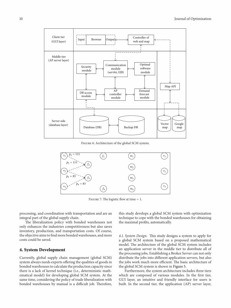Start

Solve a global SCM model

BOM table Demand forecasting

Visualize results(global SCM system)

End

Decide the number of nodes(upstream midstream and downstream)

Figure 1 A flow chart of the proposed procedure

Vendor Facility Warehouse Retailer

1

2

3

f1

f2

w1

w2

r1

r2

r3

Figure 2 Schema of a global SCM

bonded warehouse is one building or another secured areawhere dutiable goods may be stored or processed withoutpayment of duty It may be managed by the state or bya private enterprise The liberalization policy with bondedwarehouses not only enhances the industries competitivenessbut also saves inventory production and transportation costsOf course the objective is to find more bonded warehousesand more costs can be saved In this study the policy hasproved the advantage for the exporter obtaining more profitin our numerical examples [24ndash28]

A global SCM is seen as a network that includesupstreammidstream and downstream sectors linkage wherewe consider vendors as upstream facilities and warehousesas midstream and retailers (or customers) as downstreamThe liberalization policy focuses on bonded warehouses ofmidstream in different countries around the world is notconsidered in the current SCM model [7 29] In this studywe then propose a global SCM model to be suitable forthe international liberalization policy The objective is tomaximize the profits associated with inventory productiontranspiration and distribution in the period of times The

global SCM model is formed as a linear mixed-integerprogram and solved by commerce software (ie [30])Then aflow chart for the proposed procedure is depicted in Figure 1

This paper is organized as follows Section 2 definesthe notations in global SCM and forms a basic model ofglobal SCM Section 3 describes a procedure of global SCMSection 4 shows the system architecture of a global SCMFinally numerical examples demonstrate that the proposedglobal SCMmethod can enhance profit ratio in Section 5

2 A Global SCM Model

There are four stages in the global SCM environment dis-cussed the vendor facility warehouse and retailer Eachstage may be located in different nations around the worldThe general structure of a global supply chain network hasbeen displayed in Figure 2 For simplifying presentation bothincome and cost statements occur in the dashed rectangle asfollows

(i) Income statement

(a) sales of goods in warehouse(b) transfer price of goods in facility

(ii) Cost statement

(a) procurement cost from vendor(b) transportation cost (ie vendor to facility facil-

ity to warehouse and warehouse to retailer)(c) inventory cost (ie warehouse)

Notations are described in Section 21 and a basic modelof global SCM is formulated in Section 22

21 Notations There are seven entity sets

119873 The set of nations 119899

119881 The set of vendors 119907

119865 The set of facilities 119891

119882 The set of warehouses 119908

119877 The set of retailers 119903

119879 The set of times 119905

119875 The set of parts (or goods) 119901

for presenting each entity associated with notations as shownabove

All parameters are composite style which are composedof uppercase English strings and suffixes with one or morelowercase alphabet characters and each suffix single lower-case alphabet character presents the element of relative entitysets These parameters are

119875119877119868119862119864119908119901 The sales price of part 119901 in warehouse 119908

119879119875119877119868119862119864119891119901 The transfer price of part 119901 in facility 119891

119875119875119877119868119862119864V119901 The procurement cost of part 119901 fromvendor V













1198911015840



retailer 119903119879119887119900119898



1199011015840













119877 119880119891119908119901




warehouse 119908





time 119905



119877119905119891119908119901


119877119905119908119903119901



119868119905119908119901








119877119861119905119891119908119901



time 119905


119905119899 119894119887119905minus

119905119899 and



Maximize sum

119905isin119879 119899isin119873

((1 minus 119879119860119883119899) 119894119887119905+

119905119899minus 119894119887119905minus

119905119899) (1)

subject to

119894119887119905+

119905119899minus 119894119887119905minus

119905119899

= sum

119901

( sum

119908isin119882 119903isin119877 119901isin119875

(119877119905119908119903119901

lowast

(119875119877119868119862119864119908119901

minus 119875119879119901

lowast 119879119862119874119878119879119908119903

))

(2)


minus sum

119891isin119865119908isin119882 119901isin119875

(119877119905119891119908119901

lowast (119879119875119877119868119862119864119891119901

+ 119875119879119901

lowast 119879119862119874119878119879119891119908

))

(3)

minus sum

119891isin119865119908isin119882119901isin119875

((119877119905119891119908119901

minus 119877119861119905119891119908119901

)

lowast 119879119875119877119868119862119864119891119901

lowast 119863119880119879119884119899119901

)

(4)

minus sum

119908isin119882119901isin119875

(119868119905119908119901

lowast 119875119868119901

lowast 119868119862119874119878119879119908

) (5)

minus sum

119908isin119882

(119865119862119874119878119879119908

) (6)

+ sum

119891isin119865119908isin119882119901isin119875

(119877119905119891119908119901

lowast 119879119875119877119868119862119864119891119901

) (7)

+ sum

1198911015840119891isin119865119891

1015840= 119891119901isin119875

(1198771199051198911198911015840119901

lowast 119879119875119877119868119862119864119891119901

) (8)

minus sum

1198911015840119891isin119865119891

1015840= 119891119901isin119875

(1198771199051198911015840119891119901

lowast (1198791198751198771198681198621198641198911015840119901

+119875119879119901

lowast 1198791198621198741198781198791198911015840119891))

(9)

minus sum

1198911015840119891isin119865119891

1015840= 119891119901isin119875

((1198771199051198911015840119891119901

minus 1198771198611199051198911015840119891119901

)

lowast1198791198751198771198681198621198641198911015840119901

lowast 119863119880119879119884119899119901

)

(10)

minus sum

Visin119881119891isin119865119901isin119875

(119877119905V119891119901

lowast (119875119875119877119868119862119864V119901 + 119875119879119901

lowast 119879119862119874119878119879V119891))

(11)

minus sum

Visin119881119891isin119865119901isin119875

((119877119905V119891119901 minus 119877119861

119905V119891119901)

lowast119875119875119877119868119862119864V119901 lowast 119863119880119879119884119899119901

)

(12)

minus sum

119891isin119865119901isin119875

(119872119905119891119901

lowast 119872119862119874119878119879119891119901

) (13)

minus sum

119891isin119865119901isin119875

(119868119905119891119901

lowast PI119901

lowast 119868119862119874119878119879119891) (14)

minus sum

119891isin119865119901isin119875

(119865119862119874119878119879119891)) for 119905 isin 119879 119899 isin 119873 (15)




Income Statement




Cost Statement


to warehouse 119908





to warehouse 119908


1015840







We have

119868119905119891119901

+ sum

Visin119881

119877(119905minus119879V119891)V119891119901

+ sum

1198911015840isin119865 1198911015840= 119891

119877(119905minus1198791198911015840119891)1198911015840119891119901

+ 119872(119905minus119879119887119900119898

119891119901)119891119901

minus sum

1199011015840isin119875 119901 = 119901

1015840

BOM1199011015840119901

lowast 1198721199051198911199011015840 minus sum

1198911015840isin1198651198911015840= 119891

1198771199051198911198911015840119901

minus sum

119908isin119882

119877119905119891119908119901

= 119868(119905+1)119891119901


(16)


119868119905119908119901

+ sum

119891isin119865

119877(119905minus119879119891119908)119891119908119901

minus sum

119903isin119877

119877119905119908119903119901

= 119868(119905+1)119908119901


(17)

119868119861119905119891119901

+ sum

Visin119881

119877119861(119905minus119879V119891)V119891119901

+ sum

1198911015840isin1198651198911015840= 119891

119877119861(119905minus1198791198911015840119891)1198911015840119891119901

+ 119872119861(119905minus119879119887119900119898

119891119901)119891119901 minus sum

1199011015840isin1198751199011015840= 119901

BOM1199011015840119901

lowast 1198721198611199051198911199011015840

minus sum

1198911015840

1198771198611199051198911198911015840119901

minus sum

119908

119877119861119905119891119908119901

= 119868119861(119905+1)119891119901


(18)

119868119861119905119908119901

+ sum

119891isin119865

119877119861(119905minus119879119891119908)119891119908119901

minus sum

119903isin119877

119877119905119908119903119901

= 119868119861(119905+1)119908119901


(19)

sum

119908isin119882

119877(119905minus119879119908119903)119908119903119901

= 119863119905119903119901





119872119905119891119901

le 119872 119880119891119901

(21)

119868119905119891119901

le 119868 119880119891119901

(22)

119868119905119908119901

le 119868 119880119908119901

(23)

119877119905V119891119901 le 119877 119880V119891119901 (24)

1198771199051198911198911015840119901

le 119877 1198801198911198911015840119901 (25)

119877119905119891119908119901

le 119877 119880119891119908119901

(26)

119877119905119908119903119901

le 119877 119880119908119903119901

(27)

119877119861119905V119891119901 le 119877

119905V119891119901 (28)

1198771198611199051198911198911015840119901

le 1198771199051198911198911015840119901 (29)

119877119861119905119891119908119901

le 119877119905119891119908119901

(30)

for 119905 isin 119879 V isin 119881 119891 1198911015840


119903 isin 119877





119871119874119862V V1

V2

V3



119871119874119862119891

1198911

1198912

1198913

1198914



119871119874119862119908

1199081

1199082

1199083

1199084



119871119874119862119903

1199031

1199032

1199033



119875119879119901

1199011

1199012

1199013

1199014

1199015

Weighting 1 02 08 01 05














119875119868119901

1199011

1199012

1199013

1199014

1199015

Weighting 05 01 05 01 04


119863119880119879119884119899119901

1199011

1199012

1199013

1199014

1199015

1198991

02 03 02 001 0051198992

03 002 03 001 011198993

01 001 01 005 003


119879119886119909119899

1198991

1198992

1198993

007 003 008


119875119875119877119868119862119864V119901 1199011

1199012

1199013

1199014

1199015

V1

28V2

40V3



119877 119880V119891119901 1198911

1198912

1198913

1198914

V1

0 1199014

= 1000 0 0V2

0 0 1199015

= 500 1199015

= 500

V3

1199012

= 750 1199014

= 1500 0 1199013

= 1500 1199012

= 700



119872119862119874119878119879119891119901119872 119880

1198911199011199011

1199012

1199013

1199014

1199015

1198911

204001198912

303501198913

283001198914



119879119862119874119878119879V119891119879V119891 1198911

1198912

1198913

1198914

V1

31V2

11 11V3

42 31 21




119861119874119872 1199011015840

11199011015840

21199011015840

31199011015840

41199011015840

5

1199011

0 2 1 0 01199012

0 0 0 0 01199013

0 0 0 1 11199014

0 0 0 0 01199015

0 0 0 0 0



119879119887119900119898119891119901

119879119875119877119868119862119864119891119901

1199011

1199012

1199013

1199014

1199015

1198911

12501198912

11501198913

11501198914



119868119862119874119878119879119891

1198911

1198912

1198913

1198914

6 2 1 12


119868 119880119891119901

1199011

1199012

1199013

1199014

1199015

1198911

200 400 200 0 01198912

0 0 300 300 3001198913

0 0 400 400 4001198914

100 200 100 0 0


11987911986211987411987811987911989111989110158401198791198911198911015840 119891

11198912

1198913

1198914

1198911

1198912

221198913

321198914



119877 1198801198911198911015840119901

1198911

1198912

1198913

1198914

1198911

0 0 0 01198912

1199013

= 1000 0 0 01198913

0 0 0 1199013

= 1000

1198914

0 0 0 0




119868119862119874119878119879119908

(119865119862119874119878119879119908)

1199081

1199082

1199083

1199084

5 (50) 1 (10) 1 (10) 10 (100)


119879119862119874119878119879119891119908

119879119891119908

1199081

1199082

1199083

1199084

1198911

111198912

21 11198913

111198914



119877 119880119891119908119901

1199081

1199082

1199083

1199084

1198911

1199011

= 800 0 0 01198912

1199013

= 800 1199013

= 600 0 01198913

0 0 1199013

= 1000 01198914

1199011

= 700 0 0 0


119879119862119874119878119879119908119903

(119879119908119903

) 1199031

1199032

1199033

1199081

1 (1) 3 (1)1199082

2 (2) 1 (1)1199083

1 (1)1199084



119877 119880119908119903119901

1199031

1199032

1199033

1199081

1199011

= 700 1199013

= 800 0 1199011

= 300

1199082

1199013

= 800 1199013

= 8000 01199083

0 1199013

= 800 01199084

0 0 1199011

= 1000


119875119877119868119862119864119908119901

119868 119880119908119901

1199011

1199012

1199013

1199014

1199015

1199081

380300 0 280300 0 01199082

0 0 200500 0 01199083

0 0 200600 0 01199084

450150 0 0 0 0

119879119891 119861119900119898

+ [1198791198911198911015840 + 119879119891 119861119900119898

] + 119879119891119908

+ 119879119908119903


1198911198911015840 + 1198791198911015840119861119900119898





Min119879

sum

119905=1

1003816100381610038161003816119878119905 minus (119886 + 119887119876119905) 119910119905

1003816100381610038161003816(31)

st 119910119905

= 1199101199051015840 (forall119905 119905

1015840 and 119905 = 1199051015840

which mean


(32)

119896

sum

119905=1

119910119905

= 119896 (33)

119910119905


(34)






(119886 119910119905) = 119886119910


1119905(119886 119910119905) which

is equal to 1198651119905

(119886 119910119905) (ie 119891

1119905(1198861198971

1198861199051198972

) = 1198651119905

(119886 119910119905) at each


119905)


1119905(119886 119910119905)


Let

1198911119905

(119886 119910119905) = 119886119910

119905cong 120572119905

=

119898+1

sum

1198971=1

119898+1

sum

1198972=1

1198651119894

(11988911198971

11988921199051198972

) 12059611989711198972

(35)

119886 =

119898+1

sum

1198971=1

119898+1

sum

1198972=1

11988911198971

12059611989711198972

(36)



Retailer 1198771

Retailer 1198772

Retailer 1198773

119863119905119903119901

1199011

1199012

1199013

1199014

1199015

1199011

1199012

1199013

1199014

1199015

1199011

1199012

1199013

1199014

1199015

119905 = 1 0 0 0 0 0 0 0 0 0 0 0 0 0 0 0119905 = 2 0 0 0 0 0 0 0 0 0 0 0 0 0 0 0119905 = 3 0 0 0 0 0 0 0 0 0 0 0 0 0 0 0119905 = 4 0 0 0 0 0 0 0 0 0 0 0 0 0 0 0119905 = 5 0 0 0 0 0 0 0 0 0 0 0 0 0 0 0119905 = 6 0 0 180 0 0 0 0 120 0 0 0 0 0 0 0119905 = 7 0 0 190 0 0 0 0 110 0 0 0 0 0 0 0119905 = 8 52 0 170 0 0 0 0 100 0 0 83 0 0 0 0119905 = 9 38 0 160 0 0 0 0 130 0 0 90 0 0 0 0119905 = 10 60 0 210 0 0 0 0 120 0 0 50 0 0 0 0119905 = 11 43 0 180 0 0 0 0 110 0 0 60 0 0 0 0119905 = 12 52 0 190 0 0 0 0 100 0 0 76 0 0 0 0119905 = 13 56 0 170 0 0 0 0 110 0 0 56 0 0 0 0119905 = 14 48 0 180 0 0 0 0 130 0 0 76 0 0 0 0119905 = 15 58 0 200 0 0 0 0 120 0 0 99 0 0 0 0119905 = 16 31 0 190 0 0 0 0 90 0 0 80 0 0 0 0119905 = 17 52 0 180 0 0 0 0 120 0 0 50 0 0 0 0


Reproduce

Parts(materials)

Semi finishedgoods

Finished goods


Tf Tfw Trw

Tff998400

BOMp998400p

Facilityrsquo


119910119905

=

119898+1

sum

1198971=1

119898+1

sum

1198972=1

11988921199051198972

12059611989711198972

(37)

119898+1

sum

1198971=1

119898+1

sum

1198972=1

12059611989711198972

= 1 (38)

119898

sum

1198971=1

119898

sum

1198972=1

(11990611989711198972

+ V11989711198972

) = 1 (39)

12059611989711198972

+ 12059611989711198972+1

+ 1205961198971+11198972+1

ge 1199061198971 1198972

for 1198971

= 1 119898

1198972

= 1 119898

(40)

12059611989711198972

+ 1205961198971+11198972

+ 1205961198971+11198972+1

ge V11989711198972

for 1198971

= 1 119898

1198972

= 1 119898

(41)

where 12059611989711198972

ge 0 and 11990611989711198972

V11989711198972


119905) as the con-



= 1 then 12059611989711198972

+

12059611989711198972+1

+ 1205961198971+11198972+1

= 1 and 1198911119905

(119886 119910119905) = 1198651119905

(11988911198971

11988921199051198972

)12059611989711198972

+

1198651119905

(11988911198971

11988921199051198972+1

)12059611989711198972+1

+ 1198651119905

(11988911198971+1

11988921199051198972+1

)1205961198971+11198972+1 or if

V11989711198972

= 1 then 12059611989711198972

+ 1205961198971+11198972

+ 1205961198971+11198972+1

= 1 and1198911119905

(119886 119910119905) = 119865

1119905(11988911198971

11988921199051198972

)12059611989711198972

+ 1198651119905

(11988911198971+1

11988921199051198972

)1205961198971+11198972

+

1198651119905

(11988911198971+1

11988921199051198972+1

)1205961198971+11198972+1


1119905(119886 119910119905) = 119886119910

119905cong 120572119905

Similarly 1198652119905

(119887 119910119905) = 119887119910




Min119879

sum

119905=1

Φ119905

(42)

st (32) and (33) (43)


Parts

2 1

1 1

0

p1

p1

p2

p2

p3

p3

p4

p4

p5

p5

minus

minus minus

minus minus

minus minus minus

minus minus minus

minusminus

minus

minus

minus

minus

minus

minus

minus

Figure 4 BOM figure

Middle-tier


End users

End user 3

End user 1

End user 2

applicationserver 1

Middle-tier

Data baseBackup DB

applicationserver 2


servers


(119906119905minus 1) 119872 + 119878

119905minus (120572119905+ 120573119905119876119905)

le Φ119905

le 119878119905minus (120572119905+ 120573119905119876119905) + (1 minus 119906

119905) 119872

(44)

minus 119906119905119872 + (120572

119905+ 120573119905119876119905) minus 119878119905

le Φ119905

le (120572119905+ 120573119905119876119905) minus 119878119905+ 119906119905119872

(45)


isin 0 1 Φ119905

ge 0 120572119905 and


119905and 119887119910

119905 respectively



(i) If 119906119905

= 1 then Φ119905



ge 0(ii) If 119906

119905= 0 then Φ



ge 0






5can produce a p

3 and a p

3with








(GUI layer)

Security module



AP controller

module


Backup DB



Communicationmodule

(servlet EJB)

Google map

Map API

Database (DB)

DB access module

Vector map


f1

f2

f3

f4

w1

w2

w3

w4

r1

r2

r3

1

2

3

p4 = 111

p5 = 111

p5 = 83

p4 = 83










p5 = 111

p5 = 83

p4 = 83

p4 = 111

p4 = 279

p5 = 279

p5 = 90

p4 = 90

f1

f2

f3

f4

w1

w2

w3

w4

r1

r2

r3

1

2

3


p1 = 52

p2 = 76

p5 = 76

p3 = 60

p3 = 90

p3 = 110 p3 = 110

p3 = 120

p3 = 180p3 = 190

p3 = 190

p2 = 180

p1 = 83p4 = 76

p4 = 56

p3 = 38

p3 = 170

p3 = 110

p4 = 386

p5 = 386

p5 = 56

p2 = 86

p2 = 100

p4 = 342

p5 = 342

p3 = 43f1

f2

f3

f4

w1

w2

w3

w4

r1

r2

r3

1

2

3


p4 = 338

p4 = 386 p3 = 52

p5 = 386p5 = 338

p5 = 76

p4 = 76

p2 = 104

p2 = 120p2 = 100

p5 = 56

p4 = 56

p3 = 60

p3 = 60

p3 = 50

p1 = 90 p1 = 83 p1 = 83

p1 = 52p1 = 38

p3 = 110

p1 = 190

p3 = 100p3 = 100

p3 = 170p3 = 160

p3 = 130

p2 = 120

f1

f2

f3

f4

w1

w2

w3

w4

r1

r2

r3

1

2

3

p3 = 170 p1 = 52






1 1198912 1198913 1198914) four


1 1199032 1199033) Under








f1

f2

f3

f4

w1

w2

w3

w4

r1

r2

r3

1

2

3

p4 = 348

p5 = 348

p2 = 112

p2 = 152p2 = 120

p4 = 99p4 = 76

p5 = 76

p3 = 56

p3 = 210

p3 = 120

p1 = 38p1 = 60

p2 = 86

p3 = 60

p1 = 50 p1 = 90 p1 = 90p1 = 83

p3 = 100

p3 = 130

p3 = 160

p3 = 43

p3 = 56

p3 = 130

p5 = 99

p4 = 338

p5 = 338

p3 = 160 p1 = 38

p3 = 170 p1 = 52


146

153

163177

181

187

191

196

204 237

251

0

5

10

15

20

25

30


Ratio

()

Benefit ratio












6 Conclusions



Appendix


Acknowledgments


References











































Volume 2014




Journal of











Journal of


Function Spaces






Algebra





















1198911015840



retailer 119903119879119887119900119898



1199011015840













119877 119880119891119908119901




warehouse 119908





time 119905



119877119905119891119908119901


119877119905119908119903119901



119868119905119908119901








119877119861119905119891119908119901



time 119905


119905119899 119894119887119905minus

119905119899 and



Maximize sum

119905isin119879 119899isin119873

((1 minus 119879119860119883119899) 119894119887119905+

119905119899minus 119894119887119905minus

119905119899) (1)

subject to

119894119887119905+

119905119899minus 119894119887119905minus

119905119899

= sum

119901

( sum

119908isin119882 119903isin119877 119901isin119875

(119877119905119908119903119901

lowast

(119875119877119868119862119864119908119901

minus 119875119879119901

lowast 119879119862119874119878119879119908119903

))

(2)


minus sum

119891isin119865119908isin119882 119901isin119875

(119877119905119891119908119901

lowast (119879119875119877119868119862119864119891119901

+ 119875119879119901

lowast 119879119862119874119878119879119891119908

))

(3)

minus sum

119891isin119865119908isin119882119901isin119875

((119877119905119891119908119901

minus 119877119861119905119891119908119901

)

lowast 119879119875119877119868119862119864119891119901

lowast 119863119880119879119884119899119901

)

(4)

minus sum

119908isin119882119901isin119875

(119868119905119908119901

lowast 119875119868119901

lowast 119868119862119874119878119879119908

) (5)

minus sum

119908isin119882

(119865119862119874119878119879119908

) (6)

+ sum

119891isin119865119908isin119882119901isin119875

(119877119905119891119908119901

lowast 119879119875119877119868119862119864119891119901

) (7)

+ sum

1198911015840119891isin119865119891

1015840= 119891119901isin119875

(1198771199051198911198911015840119901

lowast 119879119875119877119868119862119864119891119901

) (8)

minus sum

1198911015840119891isin119865119891

1015840= 119891119901isin119875

(1198771199051198911015840119891119901

lowast (1198791198751198771198681198621198641198911015840119901

+119875119879119901

lowast 1198791198621198741198781198791198911015840119891))

(9)

minus sum

1198911015840119891isin119865119891

1015840= 119891119901isin119875

((1198771199051198911015840119891119901

minus 1198771198611199051198911015840119891119901

)

lowast1198791198751198771198681198621198641198911015840119901

lowast 119863119880119879119884119899119901

)

(10)

minus sum

Visin119881119891isin119865119901isin119875

(119877119905V119891119901

lowast (119875119875119877119868119862119864V119901 + 119875119879119901

lowast 119879119862119874119878119879V119891))

(11)

minus sum

Visin119881119891isin119865119901isin119875

((119877119905V119891119901 minus 119877119861

119905V119891119901)

lowast119875119875119877119868119862119864V119901 lowast 119863119880119879119884119899119901

)

(12)

minus sum

119891isin119865119901isin119875

(119872119905119891119901

lowast 119872119862119874119878119879119891119901

) (13)

minus sum

119891isin119865119901isin119875

(119868119905119891119901

lowast PI119901

lowast 119868119862119874119878119879119891) (14)

minus sum

119891isin119865119901isin119875

(119865119862119874119878119879119891)) for 119905 isin 119879 119899 isin 119873 (15)




Income Statement




Cost Statement


to warehouse 119908





to warehouse 119908


1015840







We have

119868119905119891119901

+ sum

Visin119881

119877(119905minus119879V119891)V119891119901

+ sum

1198911015840isin119865 1198911015840= 119891

119877(119905minus1198791198911015840119891)1198911015840119891119901

+ 119872(119905minus119879119887119900119898

119891119901)119891119901

minus sum

1199011015840isin119875 119901 = 119901

1015840

BOM1199011015840119901

lowast 1198721199051198911199011015840 minus sum

1198911015840isin1198651198911015840= 119891

1198771199051198911198911015840119901

minus sum

119908isin119882

119877119905119891119908119901

= 119868(119905+1)119891119901


(16)


119868119905119908119901

+ sum

119891isin119865

119877(119905minus119879119891119908)119891119908119901

minus sum

119903isin119877

119877119905119908119903119901

= 119868(119905+1)119908119901


(17)

119868119861119905119891119901

+ sum

Visin119881

119877119861(119905minus119879V119891)V119891119901

+ sum

1198911015840isin1198651198911015840= 119891

119877119861(119905minus1198791198911015840119891)1198911015840119891119901

+ 119872119861(119905minus119879119887119900119898

119891119901)119891119901 minus sum

1199011015840isin1198751199011015840= 119901

BOM1199011015840119901

lowast 1198721198611199051198911199011015840

minus sum

1198911015840

1198771198611199051198911198911015840119901

minus sum

119908

119877119861119905119891119908119901

= 119868119861(119905+1)119891119901


(18)

119868119861119905119908119901

+ sum

119891isin119865

119877119861(119905minus119879119891119908)119891119908119901

minus sum

119903isin119877

119877119905119908119903119901

= 119868119861(119905+1)119908119901


(19)

sum

119908isin119882

119877(119905minus119879119908119903)119908119903119901

= 119863119905119903119901





119872119905119891119901

le 119872 119880119891119901

(21)

119868119905119891119901

le 119868 119880119891119901

(22)

119868119905119908119901

le 119868 119880119908119901

(23)

119877119905V119891119901 le 119877 119880V119891119901 (24)

1198771199051198911198911015840119901

le 119877 1198801198911198911015840119901 (25)

119877119905119891119908119901

le 119877 119880119891119908119901

(26)

119877119905119908119903119901

le 119877 119880119908119903119901

(27)

119877119861119905V119891119901 le 119877

119905V119891119901 (28)

1198771198611199051198911198911015840119901

le 1198771199051198911198911015840119901 (29)

119877119861119905119891119908119901

le 119877119905119891119908119901

(30)

for 119905 isin 119879 V isin 119881 119891 1198911015840


119903 isin 119877





119871119874119862V V1

V2

V3



119871119874119862119891

1198911

1198912

1198913

1198914



119871119874119862119908

1199081

1199082

1199083

1199084



119871119874119862119903

1199031

1199032

1199033



119875119879119901

1199011

1199012

1199013

1199014

1199015

Weighting 1 02 08 01 05














119875119868119901

1199011

1199012

1199013

1199014

1199015

Weighting 05 01 05 01 04


119863119880119879119884119899119901

1199011

1199012

1199013

1199014

1199015

1198991

02 03 02 001 0051198992

03 002 03 001 011198993

01 001 01 005 003


119879119886119909119899

1198991

1198992

1198993

007 003 008


119875119875119877119868119862119864V119901 1199011

1199012

1199013

1199014

1199015

V1

28V2

40V3



119877 119880V119891119901 1198911

1198912

1198913

1198914

V1

0 1199014

= 1000 0 0V2

0 0 1199015

= 500 1199015

= 500

V3

1199012

= 750 1199014

= 1500 0 1199013

= 1500 1199012

= 700



119872119862119874119878119879119891119901119872 119880

1198911199011199011

1199012

1199013

1199014

1199015

1198911

204001198912

303501198913

283001198914



119879119862119874119878119879V119891119879V119891 1198911

1198912

1198913

1198914

V1

31V2

11 11V3

42 31 21




119861119874119872 1199011015840

11199011015840

21199011015840

31199011015840

41199011015840

5

1199011

0 2 1 0 01199012

0 0 0 0 01199013

0 0 0 1 11199014

0 0 0 0 01199015

0 0 0 0 0



119879119887119900119898119891119901

119879119875119877119868119862119864119891119901

1199011

1199012

1199013

1199014

1199015

1198911

12501198912

11501198913

11501198914



119868119862119874119878119879119891

1198911

1198912

1198913

1198914

6 2 1 12


119868 119880119891119901

1199011

1199012

1199013

1199014

1199015

1198911

200 400 200 0 01198912

0 0 300 300 3001198913

0 0 400 400 4001198914

100 200 100 0 0


11987911986211987411987811987911989111989110158401198791198911198911015840 119891

11198912

1198913

1198914

1198911

1198912

221198913

321198914



119877 1198801198911198911015840119901

1198911

1198912

1198913

1198914

1198911

0 0 0 01198912

1199013

= 1000 0 0 01198913

0 0 0 1199013

= 1000

1198914

0 0 0 0




119868119862119874119878119879119908

(119865119862119874119878119879119908)

1199081

1199082

1199083

1199084

5 (50) 1 (10) 1 (10) 10 (100)


119879119862119874119878119879119891119908

119879119891119908

1199081

1199082

1199083

1199084

1198911

111198912

21 11198913

111198914



119877 119880119891119908119901

1199081

1199082

1199083

1199084

1198911

1199011

= 800 0 0 01198912

1199013

= 800 1199013

= 600 0 01198913

0 0 1199013

= 1000 01198914

1199011

= 700 0 0 0


119879119862119874119878119879119908119903

(119879119908119903

) 1199031

1199032

1199033

1199081

1 (1) 3 (1)1199082

2 (2) 1 (1)1199083

1 (1)1199084



119877 119880119908119903119901

1199031

1199032

1199033

1199081

1199011

= 700 1199013

= 800 0 1199011

= 300

1199082

1199013

= 800 1199013

= 8000 01199083

0 1199013

= 800 01199084

0 0 1199011

= 1000


119875119877119868119862119864119908119901

119868 119880119908119901

1199011

1199012

1199013

1199014

1199015

1199081

380300 0 280300 0 01199082

0 0 200500 0 01199083

0 0 200600 0 01199084

450150 0 0 0 0

119879119891 119861119900119898

+ [1198791198911198911015840 + 119879119891 119861119900119898

] + 119879119891119908

+ 119879119908119903


1198911198911015840 + 1198791198911015840119861119900119898





Min119879

sum

119905=1

1003816100381610038161003816119878119905 minus (119886 + 119887119876119905) 119910119905

1003816100381610038161003816(31)

st 119910119905

= 1199101199051015840 (forall119905 119905

1015840 and 119905 = 1199051015840

which mean


(32)

119896

sum

119905=1

119910119905

= 119896 (33)

119910119905


(34)






(119886 119910119905) = 119886119910


1119905(119886 119910119905) which

is equal to 1198651119905

(119886 119910119905) (ie 119891

1119905(1198861198971

1198861199051198972

) = 1198651119905

(119886 119910119905) at each


119905)


1119905(119886 119910119905)


Let

1198911119905

(119886 119910119905) = 119886119910

119905cong 120572119905

=

119898+1

sum

1198971=1

119898+1

sum

1198972=1

1198651119894

(11988911198971

11988921199051198972

) 12059611989711198972

(35)

119886 =

119898+1

sum

1198971=1

119898+1

sum

1198972=1

11988911198971

12059611989711198972

(36)



Retailer 1198771

Retailer 1198772

Retailer 1198773

119863119905119903119901

1199011

1199012

1199013

1199014

1199015

1199011

1199012

1199013

1199014

1199015

1199011

1199012

1199013

1199014

1199015

119905 = 1 0 0 0 0 0 0 0 0 0 0 0 0 0 0 0119905 = 2 0 0 0 0 0 0 0 0 0 0 0 0 0 0 0119905 = 3 0 0 0 0 0 0 0 0 0 0 0 0 0 0 0119905 = 4 0 0 0 0 0 0 0 0 0 0 0 0 0 0 0119905 = 5 0 0 0 0 0 0 0 0 0 0 0 0 0 0 0119905 = 6 0 0 180 0 0 0 0 120 0 0 0 0 0 0 0119905 = 7 0 0 190 0 0 0 0 110 0 0 0 0 0 0 0119905 = 8 52 0 170 0 0 0 0 100 0 0 83 0 0 0 0119905 = 9 38 0 160 0 0 0 0 130 0 0 90 0 0 0 0119905 = 10 60 0 210 0 0 0 0 120 0 0 50 0 0 0 0119905 = 11 43 0 180 0 0 0 0 110 0 0 60 0 0 0 0119905 = 12 52 0 190 0 0 0 0 100 0 0 76 0 0 0 0119905 = 13 56 0 170 0 0 0 0 110 0 0 56 0 0 0 0119905 = 14 48 0 180 0 0 0 0 130 0 0 76 0 0 0 0119905 = 15 58 0 200 0 0 0 0 120 0 0 99 0 0 0 0119905 = 16 31 0 190 0 0 0 0 90 0 0 80 0 0 0 0119905 = 17 52 0 180 0 0 0 0 120 0 0 50 0 0 0 0


Reproduce

Parts(materials)

Semi finishedgoods

Finished goods


Tf Tfw Trw

Tff998400

BOMp998400p

Facilityrsquo


119910119905

=

119898+1

sum

1198971=1

119898+1

sum

1198972=1

11988921199051198972

12059611989711198972

(37)

119898+1

sum

1198971=1

119898+1

sum

1198972=1

12059611989711198972

= 1 (38)

119898

sum

1198971=1

119898

sum

1198972=1

(11990611989711198972

+ V11989711198972

) = 1 (39)

12059611989711198972

+ 12059611989711198972+1

+ 1205961198971+11198972+1

ge 1199061198971 1198972

for 1198971

= 1 119898

1198972

= 1 119898

(40)

12059611989711198972

+ 1205961198971+11198972

+ 1205961198971+11198972+1

ge V11989711198972

for 1198971

= 1 119898

1198972

= 1 119898

(41)

where 12059611989711198972

ge 0 and 11990611989711198972

V11989711198972


119905) as the con-



= 1 then 12059611989711198972

+

12059611989711198972+1

+ 1205961198971+11198972+1

= 1 and 1198911119905

(119886 119910119905) = 1198651119905

(11988911198971

11988921199051198972

)12059611989711198972

+

1198651119905

(11988911198971

11988921199051198972+1

)12059611989711198972+1

+ 1198651119905

(11988911198971+1

11988921199051198972+1

)1205961198971+11198972+1 or if

V11989711198972

= 1 then 12059611989711198972

+ 1205961198971+11198972

+ 1205961198971+11198972+1

= 1 and1198911119905

(119886 119910119905) = 119865

1119905(11988911198971

11988921199051198972

)12059611989711198972

+ 1198651119905

(11988911198971+1

11988921199051198972

)1205961198971+11198972

+

1198651119905

(11988911198971+1

11988921199051198972+1

)1205961198971+11198972+1


1119905(119886 119910119905) = 119886119910

119905cong 120572119905

Similarly 1198652119905

(119887 119910119905) = 119887119910




Min119879

sum

119905=1

Φ119905

(42)

st (32) and (33) (43)


Parts

2 1

1 1

0

p1

p1

p2

p2

p3

p3

p4

p4

p5

p5

minus

minus minus

minus minus

minus minus minus

minus minus minus

minusminus

minus

minus

minus

minus

minus

minus

minus

Figure 4 BOM figure

Middle-tier


End users

End user 3

End user 1

End user 2

applicationserver 1

Middle-tier

Data baseBackup DB

applicationserver 2


servers


(119906119905minus 1) 119872 + 119878

119905minus (120572119905+ 120573119905119876119905)

le Φ119905

le 119878119905minus (120572119905+ 120573119905119876119905) + (1 minus 119906

119905) 119872

(44)

minus 119906119905119872 + (120572

119905+ 120573119905119876119905) minus 119878119905

le Φ119905

le (120572119905+ 120573119905119876119905) minus 119878119905+ 119906119905119872

(45)


isin 0 1 Φ119905

ge 0 120572119905 and


119905and 119887119910

119905 respectively



(i) If 119906119905

= 1 then Φ119905



ge 0(ii) If 119906

119905= 0 then Φ



ge 0






5can produce a p

3 and a p

3with








(GUI layer)

Security module



AP controller

module


Backup DB



Communicationmodule

(servlet EJB)

Google map

Map API

Database (DB)

DB access module

Vector map


f1

f2

f3

f4

w1

w2

w3

w4

r1

r2

r3

1

2

3

p4 = 111

p5 = 111

p5 = 83

p4 = 83










p5 = 111

p5 = 83

p4 = 83

p4 = 111

p4 = 279

p5 = 279

p5 = 90

p4 = 90

f1

f2

f3

f4

w1

w2

w3

w4

r1

r2

r3

1

2

3


p1 = 52

p2 = 76

p5 = 76

p3 = 60

p3 = 90

p3 = 110 p3 = 110

p3 = 120

p3 = 180p3 = 190

p3 = 190

p2 = 180

p1 = 83p4 = 76

p4 = 56

p3 = 38

p3 = 170

p3 = 110

p4 = 386

p5 = 386

p5 = 56

p2 = 86

p2 = 100

p4 = 342

p5 = 342

p3 = 43f1

f2

f3

f4

w1

w2

w3

w4

r1

r2

r3

1

2

3


p4 = 338

p4 = 386 p3 = 52

p5 = 386p5 = 338

p5 = 76

p4 = 76

p2 = 104

p2 = 120p2 = 100

p5 = 56

p4 = 56

p3 = 60

p3 = 60

p3 = 50

p1 = 90 p1 = 83 p1 = 83

p1 = 52p1 = 38

p3 = 110

p1 = 190

p3 = 100p3 = 100

p3 = 170p3 = 160

p3 = 130

p2 = 120

f1

f2

f3

f4

w1

w2

w3

w4

r1

r2

r3

1

2

3

p3 = 170 p1 = 52






1 1198912 1198913 1198914) four


1 1199032 1199033) Under








f1

f2

f3

f4

w1

w2

w3

w4

r1

r2

r3

1

2

3

p4 = 348

p5 = 348

p2 = 112

p2 = 152p2 = 120

p4 = 99p4 = 76

p5 = 76

p3 = 56

p3 = 210

p3 = 120

p1 = 38p1 = 60

p2 = 86

p3 = 60

p1 = 50 p1 = 90 p1 = 90p1 = 83

p3 = 100

p3 = 130

p3 = 160

p3 = 43

p3 = 56

p3 = 130

p5 = 99

p4 = 338

p5 = 338

p3 = 160 p1 = 38

p3 = 170 p1 = 52


146

153

163177

181

187

191

196

204 237

251

0

5

10

15

20

25

30


Ratio

()

Benefit ratio












6 Conclusions



Appendix


Acknowledgments


References











































Volume 2014




Journal of











Journal of


Function Spaces






Algebra










minus sum

119891isin119865119908isin119882 119901isin119875

(119877119905119891119908119901

lowast (119879119875119877119868119862119864119891119901

+ 119875119879119901

lowast 119879119862119874119878119879119891119908

))

(3)

minus sum

119891isin119865119908isin119882119901isin119875

((119877119905119891119908119901

minus 119877119861119905119891119908119901

)

lowast 119879119875119877119868119862119864119891119901

lowast 119863119880119879119884119899119901

)

(4)

minus sum

119908isin119882119901isin119875

(119868119905119908119901

lowast 119875119868119901

lowast 119868119862119874119878119879119908

) (5)

minus sum

119908isin119882

(119865119862119874119878119879119908

) (6)

+ sum

119891isin119865119908isin119882119901isin119875

(119877119905119891119908119901

lowast 119879119875119877119868119862119864119891119901

) (7)

+ sum

1198911015840119891isin119865119891

1015840= 119891119901isin119875

(1198771199051198911198911015840119901

lowast 119879119875119877119868119862119864119891119901

) (8)

minus sum

1198911015840119891isin119865119891

1015840= 119891119901isin119875

(1198771199051198911015840119891119901

lowast (1198791198751198771198681198621198641198911015840119901

+119875119879119901

lowast 1198791198621198741198781198791198911015840119891))

(9)

minus sum

1198911015840119891isin119865119891

1015840= 119891119901isin119875

((1198771199051198911015840119891119901

minus 1198771198611199051198911015840119891119901

)

lowast1198791198751198771198681198621198641198911015840119901

lowast 119863119880119879119884119899119901

)

(10)

minus sum

Visin119881119891isin119865119901isin119875

(119877119905V119891119901

lowast (119875119875119877119868119862119864V119901 + 119875119879119901

lowast 119879119862119874119878119879V119891))

(11)

minus sum

Visin119881119891isin119865119901isin119875

((119877119905V119891119901 minus 119877119861

119905V119891119901)

lowast119875119875119877119868119862119864V119901 lowast 119863119880119879119884119899119901

)

(12)

minus sum

119891isin119865119901isin119875

(119872119905119891119901

lowast 119872119862119874119878119879119891119901

) (13)

minus sum

119891isin119865119901isin119875

(119868119905119891119901

lowast PI119901

lowast 119868119862119874119878119879119891) (14)

minus sum

119891isin119865119901isin119875

(119865119862119874119878119879119891)) for 119905 isin 119879 119899 isin 119873 (15)




Income Statement




Cost Statement


to warehouse 119908





to warehouse 119908


1015840







We have

119868119905119891119901

+ sum

Visin119881

119877(119905minus119879V119891)V119891119901

+ sum

1198911015840isin119865 1198911015840= 119891

119877(119905minus1198791198911015840119891)1198911015840119891119901

+ 119872(119905minus119879119887119900119898

119891119901)119891119901

minus sum

1199011015840isin119875 119901 = 119901

1015840

BOM1199011015840119901

lowast 1198721199051198911199011015840 minus sum

1198911015840isin1198651198911015840= 119891

1198771199051198911198911015840119901

minus sum

119908isin119882

119877119905119891119908119901

= 119868(119905+1)119891119901


(16)


119868119905119908119901

+ sum

119891isin119865

119877(119905minus119879119891119908)119891119908119901

minus sum

119903isin119877

119877119905119908119903119901

= 119868(119905+1)119908119901


(17)

119868119861119905119891119901

+ sum

Visin119881

119877119861(119905minus119879V119891)V119891119901

+ sum

1198911015840isin1198651198911015840= 119891

119877119861(119905minus1198791198911015840119891)1198911015840119891119901

+ 119872119861(119905minus119879119887119900119898

119891119901)119891119901 minus sum

1199011015840isin1198751199011015840= 119901

BOM1199011015840119901

lowast 1198721198611199051198911199011015840

minus sum

1198911015840

1198771198611199051198911198911015840119901

minus sum

119908

119877119861119905119891119908119901

= 119868119861(119905+1)119891119901


(18)

119868119861119905119908119901

+ sum

119891isin119865

119877119861(119905minus119879119891119908)119891119908119901

minus sum

119903isin119877

119877119905119908119903119901

= 119868119861(119905+1)119908119901


(19)

sum

119908isin119882

119877(119905minus119879119908119903)119908119903119901

= 119863119905119903119901





119872119905119891119901

le 119872 119880119891119901

(21)

119868119905119891119901

le 119868 119880119891119901

(22)

119868119905119908119901

le 119868 119880119908119901

(23)

119877119905V119891119901 le 119877 119880V119891119901 (24)

1198771199051198911198911015840119901

le 119877 1198801198911198911015840119901 (25)

119877119905119891119908119901

le 119877 119880119891119908119901

(26)

119877119905119908119903119901

le 119877 119880119908119903119901

(27)

119877119861119905V119891119901 le 119877

119905V119891119901 (28)

1198771198611199051198911198911015840119901

le 1198771199051198911198911015840119901 (29)

119877119861119905119891119908119901

le 119877119905119891119908119901

(30)

for 119905 isin 119879 V isin 119881 119891 1198911015840


119903 isin 119877





119871119874119862V V1

V2

V3



119871119874119862119891

1198911

1198912

1198913

1198914



119871119874119862119908

1199081

1199082

1199083

1199084



119871119874119862119903

1199031

1199032

1199033



119875119879119901

1199011

1199012

1199013

1199014

1199015

Weighting 1 02 08 01 05














119875119868119901

1199011

1199012

1199013

1199014

1199015

Weighting 05 01 05 01 04


119863119880119879119884119899119901

1199011

1199012

1199013

1199014

1199015

1198991

02 03 02 001 0051198992

03 002 03 001 011198993

01 001 01 005 003


119879119886119909119899

1198991

1198992

1198993

007 003 008


119875119875119877119868119862119864V119901 1199011

1199012

1199013

1199014

1199015

V1

28V2

40V3



119877 119880V119891119901 1198911

1198912

1198913

1198914

V1

0 1199014

= 1000 0 0V2

0 0 1199015

= 500 1199015

= 500

V3

1199012

= 750 1199014

= 1500 0 1199013

= 1500 1199012

= 700



119872119862119874119878119879119891119901119872 119880

1198911199011199011

1199012

1199013

1199014

1199015

1198911

204001198912

303501198913

283001198914



119879119862119874119878119879V119891119879V119891 1198911

1198912

1198913

1198914

V1

31V2

11 11V3

42 31 21




119861119874119872 1199011015840

11199011015840

21199011015840

31199011015840

41199011015840

5

1199011

0 2 1 0 01199012

0 0 0 0 01199013

0 0 0 1 11199014

0 0 0 0 01199015

0 0 0 0 0



119879119887119900119898119891119901

119879119875119877119868119862119864119891119901

1199011

1199012

1199013

1199014

1199015

1198911

12501198912

11501198913

11501198914



119868119862119874119878119879119891

1198911

1198912

1198913

1198914

6 2 1 12


119868 119880119891119901

1199011

1199012

1199013

1199014

1199015

1198911

200 400 200 0 01198912

0 0 300 300 3001198913

0 0 400 400 4001198914

100 200 100 0 0


11987911986211987411987811987911989111989110158401198791198911198911015840 119891

11198912

1198913

1198914

1198911

1198912

221198913

321198914



119877 1198801198911198911015840119901

1198911

1198912

1198913

1198914

1198911

0 0 0 01198912

1199013

= 1000 0 0 01198913

0 0 0 1199013

= 1000

1198914

0 0 0 0




119868119862119874119878119879119908

(119865119862119874119878119879119908)

1199081

1199082

1199083

1199084

5 (50) 1 (10) 1 (10) 10 (100)


119879119862119874119878119879119891119908

119879119891119908

1199081

1199082

1199083

1199084

1198911

111198912

21 11198913

111198914



119877 119880119891119908119901

1199081

1199082

1199083

1199084

1198911

1199011

= 800 0 0 01198912

1199013

= 800 1199013

= 600 0 01198913

0 0 1199013

= 1000 01198914

1199011

= 700 0 0 0


119879119862119874119878119879119908119903

(119879119908119903

) 1199031

1199032

1199033

1199081

1 (1) 3 (1)1199082

2 (2) 1 (1)1199083

1 (1)1199084



119877 119880119908119903119901

1199031

1199032

1199033

1199081

1199011

= 700 1199013

= 800 0 1199011

= 300

1199082

1199013

= 800 1199013

= 8000 01199083

0 1199013

= 800 01199084

0 0 1199011

= 1000


119875119877119868119862119864119908119901

119868 119880119908119901

1199011

1199012

1199013

1199014

1199015

1199081

380300 0 280300 0 01199082

0 0 200500 0 01199083

0 0 200600 0 01199084

450150 0 0 0 0

119879119891 119861119900119898

+ [1198791198911198911015840 + 119879119891 119861119900119898

] + 119879119891119908

+ 119879119908119903


1198911198911015840 + 1198791198911015840119861119900119898





Min119879

sum

119905=1

1003816100381610038161003816119878119905 minus (119886 + 119887119876119905) 119910119905

1003816100381610038161003816(31)

st 119910119905

= 1199101199051015840 (forall119905 119905

1015840 and 119905 = 1199051015840

which mean


(32)

119896

sum

119905=1

119910119905

= 119896 (33)

119910119905


(34)






(119886 119910119905) = 119886119910


1119905(119886 119910119905) which

is equal to 1198651119905

(119886 119910119905) (ie 119891

1119905(1198861198971

1198861199051198972

) = 1198651119905

(119886 119910119905) at each


119905)


1119905(119886 119910119905)


Let

1198911119905

(119886 119910119905) = 119886119910

119905cong 120572119905

=

119898+1

sum

1198971=1

119898+1

sum

1198972=1

1198651119894

(11988911198971

11988921199051198972

) 12059611989711198972

(35)

119886 =

119898+1

sum

1198971=1

119898+1

sum

1198972=1

11988911198971

12059611989711198972

(36)



Retailer 1198771

Retailer 1198772

Retailer 1198773

119863119905119903119901

1199011

1199012

1199013

1199014

1199015

1199011

1199012

1199013

1199014

1199015

1199011

1199012

1199013

1199014

1199015

119905 = 1 0 0 0 0 0 0 0 0 0 0 0 0 0 0 0119905 = 2 0 0 0 0 0 0 0 0 0 0 0 0 0 0 0119905 = 3 0 0 0 0 0 0 0 0 0 0 0 0 0 0 0119905 = 4 0 0 0 0 0 0 0 0 0 0 0 0 0 0 0119905 = 5 0 0 0 0 0 0 0 0 0 0 0 0 0 0 0119905 = 6 0 0 180 0 0 0 0 120 0 0 0 0 0 0 0119905 = 7 0 0 190 0 0 0 0 110 0 0 0 0 0 0 0119905 = 8 52 0 170 0 0 0 0 100 0 0 83 0 0 0 0119905 = 9 38 0 160 0 0 0 0 130 0 0 90 0 0 0 0119905 = 10 60 0 210 0 0 0 0 120 0 0 50 0 0 0 0119905 = 11 43 0 180 0 0 0 0 110 0 0 60 0 0 0 0119905 = 12 52 0 190 0 0 0 0 100 0 0 76 0 0 0 0119905 = 13 56 0 170 0 0 0 0 110 0 0 56 0 0 0 0119905 = 14 48 0 180 0 0 0 0 130 0 0 76 0 0 0 0119905 = 15 58 0 200 0 0 0 0 120 0 0 99 0 0 0 0119905 = 16 31 0 190 0 0 0 0 90 0 0 80 0 0 0 0119905 = 17 52 0 180 0 0 0 0 120 0 0 50 0 0 0 0


Reproduce

Parts(materials)

Semi finishedgoods

Finished goods


Tf Tfw Trw

Tff998400

BOMp998400p

Facilityrsquo


119910119905

=

119898+1

sum

1198971=1

119898+1

sum

1198972=1

11988921199051198972

12059611989711198972

(37)

119898+1

sum

1198971=1

119898+1

sum

1198972=1

12059611989711198972

= 1 (38)

119898

sum

1198971=1

119898

sum

1198972=1

(11990611989711198972

+ V11989711198972

) = 1 (39)

12059611989711198972

+ 12059611989711198972+1

+ 1205961198971+11198972+1

ge 1199061198971 1198972

for 1198971

= 1 119898

1198972

= 1 119898

(40)

12059611989711198972

+ 1205961198971+11198972

+ 1205961198971+11198972+1

ge V11989711198972

for 1198971

= 1 119898

1198972

= 1 119898

(41)

where 12059611989711198972

ge 0 and 11990611989711198972

V11989711198972


119905) as the con-



= 1 then 12059611989711198972

+

12059611989711198972+1

+ 1205961198971+11198972+1

= 1 and 1198911119905

(119886 119910119905) = 1198651119905

(11988911198971

11988921199051198972

)12059611989711198972

+

1198651119905

(11988911198971

11988921199051198972+1

)12059611989711198972+1

+ 1198651119905

(11988911198971+1

11988921199051198972+1

)1205961198971+11198972+1 or if

V11989711198972

= 1 then 12059611989711198972

+ 1205961198971+11198972

+ 1205961198971+11198972+1

= 1 and1198911119905

(119886 119910119905) = 119865

1119905(11988911198971

11988921199051198972

)12059611989711198972

+ 1198651119905

(11988911198971+1

11988921199051198972

)1205961198971+11198972

+

1198651119905

(11988911198971+1

11988921199051198972+1

)1205961198971+11198972+1


1119905(119886 119910119905) = 119886119910

119905cong 120572119905

Similarly 1198652119905

(119887 119910119905) = 119887119910




Min119879

sum

119905=1

Φ119905

(42)

st (32) and (33) (43)


Parts

2 1

1 1

0

p1

p1

p2

p2

p3

p3

p4

p4

p5

p5

minus

minus minus

minus minus

minus minus minus

minus minus minus

minusminus

minus

minus

minus

minus

minus

minus

minus

Figure 4 BOM figure

Middle-tier


End users

End user 3

End user 1

End user 2

applicationserver 1

Middle-tier

Data baseBackup DB

applicationserver 2


servers


(119906119905minus 1) 119872 + 119878

119905minus (120572119905+ 120573119905119876119905)

le Φ119905

le 119878119905minus (120572119905+ 120573119905119876119905) + (1 minus 119906

119905) 119872

(44)

minus 119906119905119872 + (120572

119905+ 120573119905119876119905) minus 119878119905

le Φ119905

le (120572119905+ 120573119905119876119905) minus 119878119905+ 119906119905119872

(45)


isin 0 1 Φ119905

ge 0 120572119905 and


119905and 119887119910

119905 respectively



(i) If 119906119905

= 1 then Φ119905



ge 0(ii) If 119906

119905= 0 then Φ



ge 0






5can produce a p

3 and a p

3with








(GUI layer)

Security module



AP controller

module


Backup DB



Communicationmodule

(servlet EJB)

Google map

Map API

Database (DB)

DB access module

Vector map


f1

f2

f3

f4

w1

w2

w3

w4

r1

r2

r3

1

2

3

p4 = 111

p5 = 111

p5 = 83

p4 = 83










p5 = 111

p5 = 83

p4 = 83

p4 = 111

p4 = 279

p5 = 279

p5 = 90

p4 = 90

f1

f2

f3

f4

w1

w2

w3

w4

r1

r2

r3

1

2

3


p1 = 52

p2 = 76

p5 = 76

p3 = 60

p3 = 90

p3 = 110 p3 = 110

p3 = 120

p3 = 180p3 = 190

p3 = 190

p2 = 180

p1 = 83p4 = 76

p4 = 56

p3 = 38

p3 = 170

p3 = 110

p4 = 386

p5 = 386

p5 = 56

p2 = 86

p2 = 100

p4 = 342

p5 = 342

p3 = 43f1

f2

f3

f4

w1

w2

w3

w4

r1

r2

r3

1

2

3


p4 = 338

p4 = 386 p3 = 52

p5 = 386p5 = 338

p5 = 76

p4 = 76

p2 = 104

p2 = 120p2 = 100

p5 = 56

p4 = 56

p3 = 60

p3 = 60

p3 = 50

p1 = 90 p1 = 83 p1 = 83

p1 = 52p1 = 38

p3 = 110

p1 = 190

p3 = 100p3 = 100

p3 = 170p3 = 160

p3 = 130

p2 = 120

f1

f2

f3

f4

w1

w2

w3

w4

r1

r2

r3

1

2

3

p3 = 170 p1 = 52






1 1198912 1198913 1198914) four


1 1199032 1199033) Under








f1

f2

f3

f4

w1

w2

w3

w4

r1

r2

r3

1

2

3

p4 = 348

p5 = 348

p2 = 112

p2 = 152p2 = 120

p4 = 99p4 = 76

p5 = 76

p3 = 56

p3 = 210

p3 = 120

p1 = 38p1 = 60

p2 = 86

p3 = 60

p1 = 50 p1 = 90 p1 = 90p1 = 83

p3 = 100

p3 = 130

p3 = 160

p3 = 43

p3 = 56

p3 = 130

p5 = 99

p4 = 338

p5 = 338

p3 = 160 p1 = 38

p3 = 170 p1 = 52


146

153

163177

181

187

191

196

204 237

251

0

5

10

15

20

25

30


Ratio

()

Benefit ratio












6 Conclusions



Appendix


Acknowledgments


References











































Volume 2014




Journal of











Journal of


Function Spaces






Algebra










119868119905119908119901

+ sum

119891isin119865

119877(119905minus119879119891119908)119891119908119901

minus sum

119903isin119877

119877119905119908119903119901

= 119868(119905+1)119908119901


(17)

119868119861119905119891119901

+ sum

Visin119881

119877119861(119905minus119879V119891)V119891119901

+ sum

1198911015840isin1198651198911015840= 119891

119877119861(119905minus1198791198911015840119891)1198911015840119891119901

+ 119872119861(119905minus119879119887119900119898

119891119901)119891119901 minus sum

1199011015840isin1198751199011015840= 119901

BOM1199011015840119901

lowast 1198721198611199051198911199011015840

minus sum

1198911015840

1198771198611199051198911198911015840119901

minus sum

119908

119877119861119905119891119908119901

= 119868119861(119905+1)119891119901


(18)

119868119861119905119908119901

+ sum

119891isin119865

119877119861(119905minus119879119891119908)119891119908119901

minus sum

119903isin119877

119877119905119908119903119901

= 119868119861(119905+1)119908119901


(19)

sum

119908isin119882

119877(119905minus119879119908119903)119908119903119901

= 119863119905119903119901





119872119905119891119901

le 119872 119880119891119901

(21)

119868119905119891119901

le 119868 119880119891119901

(22)

119868119905119908119901

le 119868 119880119908119901

(23)

119877119905V119891119901 le 119877 119880V119891119901 (24)

1198771199051198911198911015840119901

le 119877 1198801198911198911015840119901 (25)

119877119905119891119908119901

le 119877 119880119891119908119901

(26)

119877119905119908119903119901

le 119877 119880119908119903119901

(27)

119877119861119905V119891119901 le 119877

119905V119891119901 (28)

1198771198611199051198911198911015840119901

le 1198771199051198911198911015840119901 (29)

119877119861119905119891119908119901

le 119877119905119891119908119901

(30)

for 119905 isin 119879 V isin 119881 119891 1198911015840


119903 isin 119877





119871119874119862V V1

V2

V3



119871119874119862119891

1198911

1198912

1198913

1198914



119871119874119862119908

1199081

1199082

1199083

1199084



119871119874119862119903

1199031

1199032

1199033



119875119879119901

1199011

1199012

1199013

1199014

1199015

Weighting 1 02 08 01 05














119875119868119901

1199011

1199012

1199013

1199014

1199015

Weighting 05 01 05 01 04


119863119880119879119884119899119901

1199011

1199012

1199013

1199014

1199015

1198991

02 03 02 001 0051198992

03 002 03 001 011198993

01 001 01 005 003


119879119886119909119899

1198991

1198992

1198993

007 003 008


119875119875119877119868119862119864V119901 1199011

1199012

1199013

1199014

1199015

V1

28V2

40V3



119877 119880V119891119901 1198911

1198912

1198913

1198914

V1

0 1199014

= 1000 0 0V2

0 0 1199015

= 500 1199015

= 500

V3

1199012

= 750 1199014

= 1500 0 1199013

= 1500 1199012

= 700



119872119862119874119878119879119891119901119872 119880

1198911199011199011

1199012

1199013

1199014

1199015

1198911

204001198912

303501198913

283001198914



119879119862119874119878119879V119891119879V119891 1198911

1198912

1198913

1198914

V1

31V2

11 11V3

42 31 21




119861119874119872 1199011015840

11199011015840

21199011015840

31199011015840

41199011015840

5

1199011

0 2 1 0 01199012

0 0 0 0 01199013

0 0 0 1 11199014

0 0 0 0 01199015

0 0 0 0 0



119879119887119900119898119891119901

119879119875119877119868119862119864119891119901

1199011

1199012

1199013

1199014

1199015

1198911

12501198912

11501198913

11501198914



119868119862119874119878119879119891

1198911

1198912

1198913

1198914

6 2 1 12


119868 119880119891119901

1199011

1199012

1199013

1199014

1199015

1198911

200 400 200 0 01198912

0 0 300 300 3001198913

0 0 400 400 4001198914

100 200 100 0 0


11987911986211987411987811987911989111989110158401198791198911198911015840 119891

11198912

1198913

1198914

1198911

1198912

221198913

321198914



119877 1198801198911198911015840119901

1198911

1198912

1198913

1198914

1198911

0 0 0 01198912

1199013

= 1000 0 0 01198913

0 0 0 1199013

= 1000

1198914

0 0 0 0




119868119862119874119878119879119908

(119865119862119874119878119879119908)

1199081

1199082

1199083

1199084

5 (50) 1 (10) 1 (10) 10 (100)


119879119862119874119878119879119891119908

119879119891119908

1199081

1199082

1199083

1199084

1198911

111198912

21 11198913

111198914



119877 119880119891119908119901

1199081

1199082

1199083

1199084

1198911

1199011

= 800 0 0 01198912

1199013

= 800 1199013

= 600 0 01198913

0 0 1199013

= 1000 01198914

1199011

= 700 0 0 0


119879119862119874119878119879119908119903

(119879119908119903

) 1199031

1199032

1199033

1199081

1 (1) 3 (1)1199082

2 (2) 1 (1)1199083

1 (1)1199084



119877 119880119908119903119901

1199031

1199032

1199033

1199081

1199011

= 700 1199013

= 800 0 1199011

= 300

1199082

1199013

= 800 1199013

= 8000 01199083

0 1199013

= 800 01199084

0 0 1199011

= 1000


119875119877119868119862119864119908119901

119868 119880119908119901

1199011

1199012

1199013

1199014

1199015

1199081

380300 0 280300 0 01199082

0 0 200500 0 01199083

0 0 200600 0 01199084

450150 0 0 0 0

119879119891 119861119900119898

+ [1198791198911198911015840 + 119879119891 119861119900119898

] + 119879119891119908

+ 119879119908119903


1198911198911015840 + 1198791198911015840119861119900119898





Min119879

sum

119905=1

1003816100381610038161003816119878119905 minus (119886 + 119887119876119905) 119910119905

1003816100381610038161003816(31)

st 119910119905

= 1199101199051015840 (forall119905 119905

1015840 and 119905 = 1199051015840

which mean


(32)

119896

sum

119905=1

119910119905

= 119896 (33)

119910119905


(34)






(119886 119910119905) = 119886119910


1119905(119886 119910119905) which

is equal to 1198651119905

(119886 119910119905) (ie 119891

1119905(1198861198971

1198861199051198972

) = 1198651119905

(119886 119910119905) at each


119905)


1119905(119886 119910119905)


Let

1198911119905

(119886 119910119905) = 119886119910

119905cong 120572119905

=

119898+1

sum

1198971=1

119898+1

sum

1198972=1

1198651119894

(11988911198971

11988921199051198972

) 12059611989711198972

(35)

119886 =

119898+1

sum

1198971=1

119898+1

sum

1198972=1

11988911198971

12059611989711198972

(36)



Retailer 1198771

Retailer 1198772

Retailer 1198773

119863119905119903119901

1199011

1199012

1199013

1199014

1199015

1199011

1199012

1199013

1199014

1199015

1199011

1199012

1199013

1199014

1199015

119905 = 1 0 0 0 0 0 0 0 0 0 0 0 0 0 0 0119905 = 2 0 0 0 0 0 0 0 0 0 0 0 0 0 0 0119905 = 3 0 0 0 0 0 0 0 0 0 0 0 0 0 0 0119905 = 4 0 0 0 0 0 0 0 0 0 0 0 0 0 0 0119905 = 5 0 0 0 0 0 0 0 0 0 0 0 0 0 0 0119905 = 6 0 0 180 0 0 0 0 120 0 0 0 0 0 0 0119905 = 7 0 0 190 0 0 0 0 110 0 0 0 0 0 0 0119905 = 8 52 0 170 0 0 0 0 100 0 0 83 0 0 0 0119905 = 9 38 0 160 0 0 0 0 130 0 0 90 0 0 0 0119905 = 10 60 0 210 0 0 0 0 120 0 0 50 0 0 0 0119905 = 11 43 0 180 0 0 0 0 110 0 0 60 0 0 0 0119905 = 12 52 0 190 0 0 0 0 100 0 0 76 0 0 0 0119905 = 13 56 0 170 0 0 0 0 110 0 0 56 0 0 0 0119905 = 14 48 0 180 0 0 0 0 130 0 0 76 0 0 0 0119905 = 15 58 0 200 0 0 0 0 120 0 0 99 0 0 0 0119905 = 16 31 0 190 0 0 0 0 90 0 0 80 0 0 0 0119905 = 17 52 0 180 0 0 0 0 120 0 0 50 0 0 0 0


Reproduce

Parts(materials)

Semi finishedgoods

Finished goods


Tf Tfw Trw

Tff998400

BOMp998400p

Facilityrsquo


119910119905

=

119898+1

sum

1198971=1

119898+1

sum

1198972=1

11988921199051198972

12059611989711198972

(37)

119898+1

sum

1198971=1

119898+1

sum

1198972=1

12059611989711198972

= 1 (38)

119898

sum

1198971=1

119898

sum

1198972=1

(11990611989711198972

+ V11989711198972

) = 1 (39)

12059611989711198972

+ 12059611989711198972+1

+ 1205961198971+11198972+1

ge 1199061198971 1198972

for 1198971

= 1 119898

1198972

= 1 119898

(40)

12059611989711198972

+ 1205961198971+11198972

+ 1205961198971+11198972+1

ge V11989711198972

for 1198971

= 1 119898

1198972

= 1 119898

(41)

where 12059611989711198972

ge 0 and 11990611989711198972

V11989711198972


119905) as the con-



= 1 then 12059611989711198972

+

12059611989711198972+1

+ 1205961198971+11198972+1

= 1 and 1198911119905

(119886 119910119905) = 1198651119905

(11988911198971

11988921199051198972

)12059611989711198972

+

1198651119905

(11988911198971

11988921199051198972+1

)12059611989711198972+1

+ 1198651119905

(11988911198971+1

11988921199051198972+1

)1205961198971+11198972+1 or if

V11989711198972

= 1 then 12059611989711198972

+ 1205961198971+11198972

+ 1205961198971+11198972+1

= 1 and1198911119905

(119886 119910119905) = 119865

1119905(11988911198971

11988921199051198972

)12059611989711198972

+ 1198651119905

(11988911198971+1

11988921199051198972

)1205961198971+11198972

+

1198651119905

(11988911198971+1

11988921199051198972+1

)1205961198971+11198972+1


1119905(119886 119910119905) = 119886119910

119905cong 120572119905

Similarly 1198652119905

(119887 119910119905) = 119887119910




Min119879

sum

119905=1

Φ119905

(42)

st (32) and (33) (43)


Parts

2 1

1 1

0

p1

p1

p2

p2

p3

p3

p4

p4

p5

p5

minus

minus minus

minus minus

minus minus minus

minus minus minus

minusminus

minus

minus

minus

minus

minus

minus

minus

Figure 4 BOM figure

Middle-tier


End users

End user 3

End user 1

End user 2

applicationserver 1

Middle-tier

Data baseBackup DB

applicationserver 2


servers


(119906119905minus 1) 119872 + 119878

119905minus (120572119905+ 120573119905119876119905)

le Φ119905

le 119878119905minus (120572119905+ 120573119905119876119905) + (1 minus 119906

119905) 119872

(44)

minus 119906119905119872 + (120572

119905+ 120573119905119876119905) minus 119878119905

le Φ119905

le (120572119905+ 120573119905119876119905) minus 119878119905+ 119906119905119872

(45)


isin 0 1 Φ119905

ge 0 120572119905 and


119905and 119887119910

119905 respectively



(i) If 119906119905

= 1 then Φ119905



ge 0(ii) If 119906

119905= 0 then Φ



ge 0






5can produce a p

3 and a p

3with








(GUI layer)

Security module



AP controller

module


Backup DB



Communicationmodule

(servlet EJB)

Google map

Map API

Database (DB)

DB access module

Vector map


f1

f2

f3

f4

w1

w2

w3

w4

r1

r2

r3

1

2

3

p4 = 111

p5 = 111

p5 = 83

p4 = 83










p5 = 111

p5 = 83

p4 = 83

p4 = 111

p4 = 279

p5 = 279

p5 = 90

p4 = 90

f1

f2

f3

f4

w1

w2

w3

w4

r1

r2

r3

1

2

3


p1 = 52

p2 = 76

p5 = 76

p3 = 60

p3 = 90

p3 = 110 p3 = 110

p3 = 120

p3 = 180p3 = 190

p3 = 190

p2 = 180

p1 = 83p4 = 76

p4 = 56

p3 = 38

p3 = 170

p3 = 110

p4 = 386

p5 = 386

p5 = 56

p2 = 86

p2 = 100

p4 = 342

p5 = 342

p3 = 43f1

f2

f3

f4

w1

w2

w3

w4

r1

r2

r3

1

2

3


p4 = 338

p4 = 386 p3 = 52

p5 = 386p5 = 338

p5 = 76

p4 = 76

p2 = 104

p2 = 120p2 = 100

p5 = 56

p4 = 56

p3 = 60

p3 = 60

p3 = 50

p1 = 90 p1 = 83 p1 = 83

p1 = 52p1 = 38

p3 = 110

p1 = 190

p3 = 100p3 = 100

p3 = 170p3 = 160

p3 = 130

p2 = 120

f1

f2

f3

f4

w1

w2

w3

w4

r1

r2

r3

1

2

3

p3 = 170 p1 = 52






1 1198912 1198913 1198914) four


1 1199032 1199033) Under








f1

f2

f3

f4

w1

w2

w3

w4

r1

r2

r3

1

2

3

p4 = 348

p5 = 348

p2 = 112

p2 = 152p2 = 120

p4 = 99p4 = 76

p5 = 76

p3 = 56

p3 = 210

p3 = 120

p1 = 38p1 = 60

p2 = 86

p3 = 60

p1 = 50 p1 = 90 p1 = 90p1 = 83

p3 = 100

p3 = 130

p3 = 160

p3 = 43

p3 = 56

p3 = 130

p5 = 99

p4 = 338

p5 = 338

p3 = 160 p1 = 38

p3 = 170 p1 = 52


146

153

163177

181

187

191

196

204 237

251

0

5

10

15

20

25

30


Ratio

()

Benefit ratio












6 Conclusions



Appendix


Acknowledgments


References











































Volume 2014




Journal of











Journal of


Function Spaces






Algebra











119875119868119901

1199011

1199012

1199013

1199014

1199015

Weighting 05 01 05 01 04


119863119880119879119884119899119901

1199011

1199012

1199013

1199014

1199015

1198991

02 03 02 001 0051198992

03 002 03 001 011198993

01 001 01 005 003


119879119886119909119899

1198991

1198992

1198993

007 003 008


119875119875119877119868119862119864V119901 1199011

1199012

1199013

1199014

1199015

V1

28V2

40V3



119877 119880V119891119901 1198911

1198912

1198913

1198914

V1

0 1199014

= 1000 0 0V2

0 0 1199015

= 500 1199015

= 500

V3

1199012

= 750 1199014

= 1500 0 1199013

= 1500 1199012

= 700



119872119862119874119878119879119891119901119872 119880

1198911199011199011

1199012

1199013

1199014

1199015

1198911

204001198912

303501198913

283001198914



119879119862119874119878119879V119891119879V119891 1198911

1198912

1198913

1198914

V1

31V2

11 11V3

42 31 21




119861119874119872 1199011015840

11199011015840

21199011015840

31199011015840

41199011015840

5

1199011

0 2 1 0 01199012

0 0 0 0 01199013

0 0 0 1 11199014

0 0 0 0 01199015

0 0 0 0 0



119879119887119900119898119891119901

119879119875119877119868119862119864119891119901

1199011

1199012

1199013

1199014

1199015

1198911

12501198912

11501198913

11501198914



119868119862119874119878119879119891

1198911

1198912

1198913

1198914

6 2 1 12


119868 119880119891119901

1199011

1199012

1199013

1199014

1199015

1198911

200 400 200 0 01198912

0 0 300 300 3001198913

0 0 400 400 4001198914

100 200 100 0 0


11987911986211987411987811987911989111989110158401198791198911198911015840 119891

11198912

1198913

1198914

1198911

1198912

221198913

321198914



119877 1198801198911198911015840119901

1198911

1198912

1198913

1198914

1198911

0 0 0 01198912

1199013

= 1000 0 0 01198913

0 0 0 1199013

= 1000

1198914

0 0 0 0




119868119862119874119878119879119908

(119865119862119874119878119879119908)

1199081

1199082

1199083

1199084

5 (50) 1 (10) 1 (10) 10 (100)


119879119862119874119878119879119891119908

119879119891119908

1199081

1199082

1199083

1199084

1198911

111198912

21 11198913

111198914



119877 119880119891119908119901

1199081

1199082

1199083

1199084

1198911

1199011

= 800 0 0 01198912

1199013

= 800 1199013

= 600 0 01198913

0 0 1199013

= 1000 01198914

1199011

= 700 0 0 0


119879119862119874119878119879119908119903

(119879119908119903

) 1199031

1199032

1199033

1199081

1 (1) 3 (1)1199082

2 (2) 1 (1)1199083

1 (1)1199084



119877 119880119908119903119901

1199031

1199032

1199033

1199081

1199011

= 700 1199013

= 800 0 1199011

= 300

1199082

1199013

= 800 1199013

= 8000 01199083

0 1199013

= 800 01199084

0 0 1199011

= 1000


119875119877119868119862119864119908119901

119868 119880119908119901

1199011

1199012

1199013

1199014

1199015

1199081

380300 0 280300 0 01199082

0 0 200500 0 01199083

0 0 200600 0 01199084

450150 0 0 0 0

119879119891 119861119900119898

+ [1198791198911198911015840 + 119879119891 119861119900119898

] + 119879119891119908

+ 119879119908119903


1198911198911015840 + 1198791198911015840119861119900119898





Min119879

sum

119905=1

1003816100381610038161003816119878119905 minus (119886 + 119887119876119905) 119910119905

1003816100381610038161003816(31)

st 119910119905

= 1199101199051015840 (forall119905 119905

1015840 and 119905 = 1199051015840

which mean


(32)

119896

sum

119905=1

119910119905

= 119896 (33)

119910119905


(34)






(119886 119910119905) = 119886119910


1119905(119886 119910119905) which

is equal to 1198651119905

(119886 119910119905) (ie 119891

1119905(1198861198971

1198861199051198972

) = 1198651119905

(119886 119910119905) at each


119905)


1119905(119886 119910119905)


Let

1198911119905

(119886 119910119905) = 119886119910

119905cong 120572119905

=

119898+1

sum

1198971=1

119898+1

sum

1198972=1

1198651119894

(11988911198971

11988921199051198972

) 12059611989711198972

(35)

119886 =

119898+1

sum

1198971=1

119898+1

sum

1198972=1

11988911198971

12059611989711198972

(36)



Retailer 1198771

Retailer 1198772

Retailer 1198773

119863119905119903119901

1199011

1199012

1199013

1199014

1199015

1199011

1199012

1199013

1199014

1199015

1199011

1199012

1199013

1199014

1199015

119905 = 1 0 0 0 0 0 0 0 0 0 0 0 0 0 0 0119905 = 2 0 0 0 0 0 0 0 0 0 0 0 0 0 0 0119905 = 3 0 0 0 0 0 0 0 0 0 0 0 0 0 0 0119905 = 4 0 0 0 0 0 0 0 0 0 0 0 0 0 0 0119905 = 5 0 0 0 0 0 0 0 0 0 0 0 0 0 0 0119905 = 6 0 0 180 0 0 0 0 120 0 0 0 0 0 0 0119905 = 7 0 0 190 0 0 0 0 110 0 0 0 0 0 0 0119905 = 8 52 0 170 0 0 0 0 100 0 0 83 0 0 0 0119905 = 9 38 0 160 0 0 0 0 130 0 0 90 0 0 0 0119905 = 10 60 0 210 0 0 0 0 120 0 0 50 0 0 0 0119905 = 11 43 0 180 0 0 0 0 110 0 0 60 0 0 0 0119905 = 12 52 0 190 0 0 0 0 100 0 0 76 0 0 0 0119905 = 13 56 0 170 0 0 0 0 110 0 0 56 0 0 0 0119905 = 14 48 0 180 0 0 0 0 130 0 0 76 0 0 0 0119905 = 15 58 0 200 0 0 0 0 120 0 0 99 0 0 0 0119905 = 16 31 0 190 0 0 0 0 90 0 0 80 0 0 0 0119905 = 17 52 0 180 0 0 0 0 120 0 0 50 0 0 0 0


Reproduce

Parts(materials)

Semi finishedgoods

Finished goods


Tf Tfw Trw

Tff998400

BOMp998400p

Facilityrsquo


119910119905

=

119898+1

sum

1198971=1

119898+1

sum

1198972=1

11988921199051198972

12059611989711198972

(37)

119898+1

sum

1198971=1

119898+1

sum

1198972=1

12059611989711198972

= 1 (38)

119898

sum

1198971=1

119898

sum

1198972=1

(11990611989711198972

+ V11989711198972

) = 1 (39)

12059611989711198972

+ 12059611989711198972+1

+ 1205961198971+11198972+1

ge 1199061198971 1198972

for 1198971

= 1 119898

1198972

= 1 119898

(40)

12059611989711198972

+ 1205961198971+11198972

+ 1205961198971+11198972+1

ge V11989711198972

for 1198971

= 1 119898

1198972

= 1 119898

(41)

where 12059611989711198972

ge 0 and 11990611989711198972

V11989711198972


119905) as the con-



= 1 then 12059611989711198972

+

12059611989711198972+1

+ 1205961198971+11198972+1

= 1 and 1198911119905

(119886 119910119905) = 1198651119905

(11988911198971

11988921199051198972

)12059611989711198972

+

1198651119905

(11988911198971

11988921199051198972+1

)12059611989711198972+1

+ 1198651119905

(11988911198971+1

11988921199051198972+1

)1205961198971+11198972+1 or if

V11989711198972

= 1 then 12059611989711198972

+ 1205961198971+11198972

+ 1205961198971+11198972+1

= 1 and1198911119905

(119886 119910119905) = 119865

1119905(11988911198971

11988921199051198972

)12059611989711198972

+ 1198651119905

(11988911198971+1

11988921199051198972

)1205961198971+11198972

+

1198651119905

(11988911198971+1

11988921199051198972+1

)1205961198971+11198972+1


1119905(119886 119910119905) = 119886119910

119905cong 120572119905

Similarly 1198652119905

(119887 119910119905) = 119887119910




Min119879

sum

119905=1

Φ119905

(42)

st (32) and (33) (43)


Parts

2 1

1 1

0

p1

p1

p2

p2

p3

p3

p4

p4

p5

p5

minus

minus minus

minus minus

minus minus minus

minus minus minus

minusminus

minus

minus

minus

minus

minus

minus

minus

Figure 4 BOM figure

Middle-tier


End users

End user 3

End user 1

End user 2

applicationserver 1

Middle-tier

Data baseBackup DB

applicationserver 2


servers


(119906119905minus 1) 119872 + 119878

119905minus (120572119905+ 120573119905119876119905)

le Φ119905

le 119878119905minus (120572119905+ 120573119905119876119905) + (1 minus 119906

119905) 119872

(44)

minus 119906119905119872 + (120572

119905+ 120573119905119876119905) minus 119878119905

le Φ119905

le (120572119905+ 120573119905119876119905) minus 119878119905+ 119906119905119872

(45)


isin 0 1 Φ119905

ge 0 120572119905 and


119905and 119887119910

119905 respectively



(i) If 119906119905

= 1 then Φ119905



ge 0(ii) If 119906

119905= 0 then Φ



ge 0






5can produce a p

3 and a p

3with








(GUI layer)

Security module



AP controller

module


Backup DB



Communicationmodule

(servlet EJB)

Google map

Map API

Database (DB)

DB access module

Vector map


f1

f2

f3

f4

w1

w2

w3

w4

r1

r2

r3

1

2

3

p4 = 111

p5 = 111

p5 = 83

p4 = 83










p5 = 111

p5 = 83

p4 = 83

p4 = 111

p4 = 279

p5 = 279

p5 = 90

p4 = 90

f1

f2

f3

f4

w1

w2

w3

w4

r1

r2

r3

1

2

3


p1 = 52

p2 = 76

p5 = 76

p3 = 60

p3 = 90

p3 = 110 p3 = 110

p3 = 120

p3 = 180p3 = 190

p3 = 190

p2 = 180

p1 = 83p4 = 76

p4 = 56

p3 = 38

p3 = 170

p3 = 110

p4 = 386

p5 = 386

p5 = 56

p2 = 86

p2 = 100

p4 = 342

p5 = 342

p3 = 43f1

f2

f3

f4

w1

w2

w3

w4

r1

r2

r3

1

2

3


p4 = 338

p4 = 386 p3 = 52

p5 = 386p5 = 338

p5 = 76

p4 = 76

p2 = 104

p2 = 120p2 = 100

p5 = 56

p4 = 56

p3 = 60

p3 = 60

p3 = 50

p1 = 90 p1 = 83 p1 = 83

p1 = 52p1 = 38

p3 = 110

p1 = 190

p3 = 100p3 = 100

p3 = 170p3 = 160

p3 = 130

p2 = 120

f1

f2

f3

f4

w1

w2

w3

w4

r1

r2

r3

1

2

3

p3 = 170 p1 = 52






1 1198912 1198913 1198914) four


1 1199032 1199033) Under








f1

f2

f3

f4

w1

w2

w3

w4

r1

r2

r3

1

2

3

p4 = 348

p5 = 348

p2 = 112

p2 = 152p2 = 120

p4 = 99p4 = 76

p5 = 76

p3 = 56

p3 = 210

p3 = 120

p1 = 38p1 = 60

p2 = 86

p3 = 60

p1 = 50 p1 = 90 p1 = 90p1 = 83

p3 = 100

p3 = 130

p3 = 160

p3 = 43

p3 = 56

p3 = 130

p5 = 99

p4 = 338

p5 = 338

p3 = 160 p1 = 38

p3 = 170 p1 = 52


146

153

163177

181

187

191

196

204 237

251

0

5

10

15

20

25

30


Ratio

()

Benefit ratio












6 Conclusions



Appendix


Acknowledgments


References











































Volume 2014




Journal of











Journal of


Function Spaces






Algebra











119868119862119874119878119879119908

(119865119862119874119878119879119908)

1199081

1199082

1199083

1199084

5 (50) 1 (10) 1 (10) 10 (100)


119879119862119874119878119879119891119908

119879119891119908

1199081

1199082

1199083

1199084

1198911

111198912

21 11198913

111198914



119877 119880119891119908119901

1199081

1199082

1199083

1199084

1198911

1199011

= 800 0 0 01198912

1199013

= 800 1199013

= 600 0 01198913

0 0 1199013

= 1000 01198914

1199011

= 700 0 0 0


119879119862119874119878119879119908119903

(119879119908119903

) 1199031

1199032

1199033

1199081

1 (1) 3 (1)1199082

2 (2) 1 (1)1199083

1 (1)1199084



119877 119880119908119903119901

1199031

1199032

1199033

1199081

1199011

= 700 1199013

= 800 0 1199011

= 300

1199082

1199013

= 800 1199013

= 8000 01199083

0 1199013

= 800 01199084

0 0 1199011

= 1000


119875119877119868119862119864119908119901

119868 119880119908119901

1199011

1199012

1199013

1199014

1199015

1199081

380300 0 280300 0 01199082

0 0 200500 0 01199083

0 0 200600 0 01199084

450150 0 0 0 0

119879119891 119861119900119898

+ [1198791198911198911015840 + 119879119891 119861119900119898

] + 119879119891119908

+ 119879119908119903


1198911198911015840 + 1198791198911015840119861119900119898





Min119879

sum

119905=1

1003816100381610038161003816119878119905 minus (119886 + 119887119876119905) 119910119905

1003816100381610038161003816(31)

st 119910119905

= 1199101199051015840 (forall119905 119905

1015840 and 119905 = 1199051015840

which mean


(32)

119896

sum

119905=1

119910119905

= 119896 (33)

119910119905


(34)






(119886 119910119905) = 119886119910


1119905(119886 119910119905) which

is equal to 1198651119905

(119886 119910119905) (ie 119891

1119905(1198861198971

1198861199051198972

) = 1198651119905

(119886 119910119905) at each


119905)


1119905(119886 119910119905)


Let

1198911119905

(119886 119910119905) = 119886119910

119905cong 120572119905

=

119898+1

sum

1198971=1

119898+1

sum

1198972=1

1198651119894

(11988911198971

11988921199051198972

) 12059611989711198972

(35)

119886 =

119898+1

sum

1198971=1

119898+1

sum

1198972=1

11988911198971

12059611989711198972

(36)



Retailer 1198771

Retailer 1198772

Retailer 1198773

119863119905119903119901

1199011

1199012

1199013

1199014

1199015

1199011

1199012

1199013

1199014

1199015

1199011

1199012

1199013

1199014

1199015

119905 = 1 0 0 0 0 0 0 0 0 0 0 0 0 0 0 0119905 = 2 0 0 0 0 0 0 0 0 0 0 0 0 0 0 0119905 = 3 0 0 0 0 0 0 0 0 0 0 0 0 0 0 0119905 = 4 0 0 0 0 0 0 0 0 0 0 0 0 0 0 0119905 = 5 0 0 0 0 0 0 0 0 0 0 0 0 0 0 0119905 = 6 0 0 180 0 0 0 0 120 0 0 0 0 0 0 0119905 = 7 0 0 190 0 0 0 0 110 0 0 0 0 0 0 0119905 = 8 52 0 170 0 0 0 0 100 0 0 83 0 0 0 0119905 = 9 38 0 160 0 0 0 0 130 0 0 90 0 0 0 0119905 = 10 60 0 210 0 0 0 0 120 0 0 50 0 0 0 0119905 = 11 43 0 180 0 0 0 0 110 0 0 60 0 0 0 0119905 = 12 52 0 190 0 0 0 0 100 0 0 76 0 0 0 0119905 = 13 56 0 170 0 0 0 0 110 0 0 56 0 0 0 0119905 = 14 48 0 180 0 0 0 0 130 0 0 76 0 0 0 0119905 = 15 58 0 200 0 0 0 0 120 0 0 99 0 0 0 0119905 = 16 31 0 190 0 0 0 0 90 0 0 80 0 0 0 0119905 = 17 52 0 180 0 0 0 0 120 0 0 50 0 0 0 0


Reproduce

Parts(materials)

Semi finishedgoods

Finished goods


Tf Tfw Trw

Tff998400

BOMp998400p

Facilityrsquo


119910119905

=

119898+1

sum

1198971=1

119898+1

sum

1198972=1

11988921199051198972

12059611989711198972

(37)

119898+1

sum

1198971=1

119898+1

sum

1198972=1

12059611989711198972

= 1 (38)

119898

sum

1198971=1

119898

sum

1198972=1

(11990611989711198972

+ V11989711198972

) = 1 (39)

12059611989711198972

+ 12059611989711198972+1

+ 1205961198971+11198972+1

ge 1199061198971 1198972

for 1198971

= 1 119898

1198972

= 1 119898

(40)

12059611989711198972

+ 1205961198971+11198972

+ 1205961198971+11198972+1

ge V11989711198972

for 1198971

= 1 119898

1198972

= 1 119898

(41)

where 12059611989711198972

ge 0 and 11990611989711198972

V11989711198972


119905) as the con-



= 1 then 12059611989711198972

+

12059611989711198972+1

+ 1205961198971+11198972+1

= 1 and 1198911119905

(119886 119910119905) = 1198651119905

(11988911198971

11988921199051198972

)12059611989711198972

+

1198651119905

(11988911198971

11988921199051198972+1

)12059611989711198972+1

+ 1198651119905

(11988911198971+1

11988921199051198972+1

)1205961198971+11198972+1 or if

V11989711198972

= 1 then 12059611989711198972

+ 1205961198971+11198972

+ 1205961198971+11198972+1

= 1 and1198911119905

(119886 119910119905) = 119865

1119905(11988911198971

11988921199051198972

)12059611989711198972

+ 1198651119905

(11988911198971+1

11988921199051198972

)1205961198971+11198972

+

1198651119905

(11988911198971+1

11988921199051198972+1

)1205961198971+11198972+1


1119905(119886 119910119905) = 119886119910

119905cong 120572119905

Similarly 1198652119905

(119887 119910119905) = 119887119910




Min119879

sum

119905=1

Φ119905

(42)

st (32) and (33) (43)


Parts

2 1

1 1

0

p1

p1

p2

p2

p3

p3

p4

p4

p5

p5

minus

minus minus

minus minus

minus minus minus

minus minus minus

minusminus

minus

minus

minus

minus

minus

minus

minus

Figure 4 BOM figure

Middle-tier


End users

End user 3

End user 1

End user 2

applicationserver 1

Middle-tier

Data baseBackup DB

applicationserver 2


servers


(119906119905minus 1) 119872 + 119878

119905minus (120572119905+ 120573119905119876119905)

le Φ119905

le 119878119905minus (120572119905+ 120573119905119876119905) + (1 minus 119906

119905) 119872

(44)

minus 119906119905119872 + (120572

119905+ 120573119905119876119905) minus 119878119905

le Φ119905

le (120572119905+ 120573119905119876119905) minus 119878119905+ 119906119905119872

(45)


isin 0 1 Φ119905

ge 0 120572119905 and


119905and 119887119910

119905 respectively



(i) If 119906119905

= 1 then Φ119905



ge 0(ii) If 119906

119905= 0 then Φ



ge 0






5can produce a p

3 and a p

3with








(GUI layer)

Security module



AP controller

module


Backup DB



Communicationmodule

(servlet EJB)

Google map

Map API

Database (DB)

DB access module

Vector map


f1

f2

f3

f4

w1

w2

w3

w4

r1

r2

r3

1

2

3

p4 = 111

p5 = 111

p5 = 83

p4 = 83










p5 = 111

p5 = 83

p4 = 83

p4 = 111

p4 = 279

p5 = 279

p5 = 90

p4 = 90

f1

f2

f3

f4

w1

w2

w3

w4

r1

r2

r3

1

2

3


p1 = 52

p2 = 76

p5 = 76

p3 = 60

p3 = 90

p3 = 110 p3 = 110

p3 = 120

p3 = 180p3 = 190

p3 = 190

p2 = 180

p1 = 83p4 = 76

p4 = 56

p3 = 38

p3 = 170

p3 = 110

p4 = 386

p5 = 386

p5 = 56

p2 = 86

p2 = 100

p4 = 342

p5 = 342

p3 = 43f1

f2

f3

f4

w1

w2

w3

w4

r1

r2

r3

1

2

3


p4 = 338

p4 = 386 p3 = 52

p5 = 386p5 = 338

p5 = 76

p4 = 76

p2 = 104

p2 = 120p2 = 100

p5 = 56

p4 = 56

p3 = 60

p3 = 60

p3 = 50

p1 = 90 p1 = 83 p1 = 83

p1 = 52p1 = 38

p3 = 110

p1 = 190

p3 = 100p3 = 100

p3 = 170p3 = 160

p3 = 130

p2 = 120

f1

f2

f3

f4

w1

w2

w3

w4

r1

r2

r3

1

2

3

p3 = 170 p1 = 52






1 1198912 1198913 1198914) four


1 1199032 1199033) Under








f1

f2

f3

f4

w1

w2

w3

w4

r1

r2

r3

1

2

3

p4 = 348

p5 = 348

p2 = 112

p2 = 152p2 = 120

p4 = 99p4 = 76

p5 = 76

p3 = 56

p3 = 210

p3 = 120

p1 = 38p1 = 60

p2 = 86

p3 = 60

p1 = 50 p1 = 90 p1 = 90p1 = 83

p3 = 100

p3 = 130

p3 = 160

p3 = 43

p3 = 56

p3 = 130

p5 = 99

p4 = 338

p5 = 338

p3 = 160 p1 = 38

p3 = 170 p1 = 52


146

153

163177

181

187

191

196

204 237

251

0

5

10

15

20

25

30


Ratio

()

Benefit ratio












6 Conclusions



Appendix


Acknowledgments


References











































Volume 2014




Journal of











Journal of


Function Spaces






Algebra











Retailer 1198771

Retailer 1198772

Retailer 1198773

119863119905119903119901

1199011

1199012

1199013

1199014

1199015

1199011

1199012

1199013

1199014

1199015

1199011

1199012

1199013

1199014

1199015

119905 = 1 0 0 0 0 0 0 0 0 0 0 0 0 0 0 0119905 = 2 0 0 0 0 0 0 0 0 0 0 0 0 0 0 0119905 = 3 0 0 0 0 0 0 0 0 0 0 0 0 0 0 0119905 = 4 0 0 0 0 0 0 0 0 0 0 0 0 0 0 0119905 = 5 0 0 0 0 0 0 0 0 0 0 0 0 0 0 0119905 = 6 0 0 180 0 0 0 0 120 0 0 0 0 0 0 0119905 = 7 0 0 190 0 0 0 0 110 0 0 0 0 0 0 0119905 = 8 52 0 170 0 0 0 0 100 0 0 83 0 0 0 0119905 = 9 38 0 160 0 0 0 0 130 0 0 90 0 0 0 0119905 = 10 60 0 210 0 0 0 0 120 0 0 50 0 0 0 0119905 = 11 43 0 180 0 0 0 0 110 0 0 60 0 0 0 0119905 = 12 52 0 190 0 0 0 0 100 0 0 76 0 0 0 0119905 = 13 56 0 170 0 0 0 0 110 0 0 56 0 0 0 0119905 = 14 48 0 180 0 0 0 0 130 0 0 76 0 0 0 0119905 = 15 58 0 200 0 0 0 0 120 0 0 99 0 0 0 0119905 = 16 31 0 190 0 0 0 0 90 0 0 80 0 0 0 0119905 = 17 52 0 180 0 0 0 0 120 0 0 50 0 0 0 0


Reproduce

Parts(materials)

Semi finishedgoods

Finished goods


Tf Tfw Trw

Tff998400

BOMp998400p

Facilityrsquo


119910119905

=

119898+1

sum

1198971=1

119898+1

sum

1198972=1

11988921199051198972

12059611989711198972

(37)

119898+1

sum

1198971=1

119898+1

sum

1198972=1

12059611989711198972

= 1 (38)

119898

sum

1198971=1

119898

sum

1198972=1

(11990611989711198972

+ V11989711198972

) = 1 (39)

12059611989711198972

+ 12059611989711198972+1

+ 1205961198971+11198972+1

ge 1199061198971 1198972

for 1198971

= 1 119898

1198972

= 1 119898

(40)

12059611989711198972

+ 1205961198971+11198972

+ 1205961198971+11198972+1

ge V11989711198972

for 1198971

= 1 119898

1198972

= 1 119898

(41)

where 12059611989711198972

ge 0 and 11990611989711198972

V11989711198972


119905) as the con-



= 1 then 12059611989711198972

+

12059611989711198972+1

+ 1205961198971+11198972+1

= 1 and 1198911119905

(119886 119910119905) = 1198651119905

(11988911198971

11988921199051198972

)12059611989711198972

+

1198651119905

(11988911198971

11988921199051198972+1

)12059611989711198972+1

+ 1198651119905

(11988911198971+1

11988921199051198972+1

)1205961198971+11198972+1 or if

V11989711198972

= 1 then 12059611989711198972

+ 1205961198971+11198972

+ 1205961198971+11198972+1

= 1 and1198911119905

(119886 119910119905) = 119865

1119905(11988911198971

11988921199051198972

)12059611989711198972

+ 1198651119905

(11988911198971+1

11988921199051198972

)1205961198971+11198972

+

1198651119905

(11988911198971+1

11988921199051198972+1

)1205961198971+11198972+1


1119905(119886 119910119905) = 119886119910

119905cong 120572119905

Similarly 1198652119905

(119887 119910119905) = 119887119910




Min119879

sum

119905=1

Φ119905

(42)

st (32) and (33) (43)


Parts

2 1

1 1

0

p1

p1

p2

p2

p3

p3

p4

p4

p5

p5

minus

minus minus

minus minus

minus minus minus

minus minus minus

minusminus

minus

minus

minus

minus

minus

minus

minus

Figure 4 BOM figure

Middle-tier


End users

End user 3

End user 1

End user 2

applicationserver 1

Middle-tier

Data baseBackup DB

applicationserver 2


servers


(119906119905minus 1) 119872 + 119878

119905minus (120572119905+ 120573119905119876119905)

le Φ119905

le 119878119905minus (120572119905+ 120573119905119876119905) + (1 minus 119906

119905) 119872

(44)

minus 119906119905119872 + (120572

119905+ 120573119905119876119905) minus 119878119905

le Φ119905

le (120572119905+ 120573119905119876119905) minus 119878119905+ 119906119905119872

(45)


isin 0 1 Φ119905

ge 0 120572119905 and


119905and 119887119910

119905 respectively



(i) If 119906119905

= 1 then Φ119905



ge 0(ii) If 119906

119905= 0 then Φ



ge 0






5can produce a p

3 and a p

3with








(GUI layer)

Security module



AP controller

module


Backup DB



Communicationmodule

(servlet EJB)

Google map

Map API

Database (DB)

DB access module

Vector map


f1

f2

f3

f4

w1

w2

w3

w4

r1

r2

r3

1

2

3

p4 = 111

p5 = 111

p5 = 83

p4 = 83










p5 = 111

p5 = 83

p4 = 83

p4 = 111

p4 = 279

p5 = 279

p5 = 90

p4 = 90

f1

f2

f3

f4

w1

w2

w3

w4

r1

r2

r3

1

2

3


p1 = 52

p2 = 76

p5 = 76

p3 = 60

p3 = 90

p3 = 110 p3 = 110

p3 = 120

p3 = 180p3 = 190

p3 = 190

p2 = 180

p1 = 83p4 = 76

p4 = 56

p3 = 38

p3 = 170

p3 = 110

p4 = 386

p5 = 386

p5 = 56

p2 = 86

p2 = 100

p4 = 342

p5 = 342

p3 = 43f1

f2

f3

f4

w1

w2

w3

w4

r1

r2

r3

1

2

3


p4 = 338

p4 = 386 p3 = 52

p5 = 386p5 = 338

p5 = 76

p4 = 76

p2 = 104

p2 = 120p2 = 100

p5 = 56

p4 = 56

p3 = 60

p3 = 60

p3 = 50

p1 = 90 p1 = 83 p1 = 83

p1 = 52p1 = 38

p3 = 110

p1 = 190

p3 = 100p3 = 100

p3 = 170p3 = 160

p3 = 130

p2 = 120

f1

f2

f3

f4

w1

w2

w3

w4

r1

r2

r3

1

2

3

p3 = 170 p1 = 52






1 1198912 1198913 1198914) four


1 1199032 1199033) Under








f1

f2

f3

f4

w1

w2

w3

w4

r1

r2

r3

1

2

3

p4 = 348

p5 = 348

p2 = 112

p2 = 152p2 = 120

p4 = 99p4 = 76

p5 = 76

p3 = 56

p3 = 210

p3 = 120

p1 = 38p1 = 60

p2 = 86

p3 = 60

p1 = 50 p1 = 90 p1 = 90p1 = 83

p3 = 100

p3 = 130

p3 = 160

p3 = 43

p3 = 56

p3 = 130

p5 = 99

p4 = 338

p5 = 338

p3 = 160 p1 = 38

p3 = 170 p1 = 52


146

153

163177

181

187

191

196

204 237

251

0

5

10

15

20

25

30


Ratio

()

Benefit ratio












6 Conclusions



Appendix


Acknowledgments


References











































Volume 2014




Journal of











Journal of


Function Spaces






Algebra










Parts

2 1

1 1

0

p1

p1

p2

p2

p3

p3

p4

p4

p5

p5

minus

minus minus

minus minus

minus minus minus

minus minus minus

minusminus

minus

minus

minus

minus

minus

minus

minus

Figure 4 BOM figure

Middle-tier


End users

End user 3

End user 1

End user 2

applicationserver 1

Middle-tier

Data baseBackup DB

applicationserver 2


servers


(119906119905minus 1) 119872 + 119878

119905minus (120572119905+ 120573119905119876119905)

le Φ119905

le 119878119905minus (120572119905+ 120573119905119876119905) + (1 minus 119906

119905) 119872

(44)

minus 119906119905119872 + (120572

119905+ 120573119905119876119905) minus 119878119905

le Φ119905

le (120572119905+ 120573119905119876119905) minus 119878119905+ 119906119905119872

(45)


isin 0 1 Φ119905

ge 0 120572119905 and


119905and 119887119910

119905 respectively



(i) If 119906119905

= 1 then Φ119905



ge 0(ii) If 119906

119905= 0 then Φ



ge 0






5can produce a p

3 and a p

3with








(GUI layer)

Security module



AP controller

module


Backup DB



Communicationmodule

(servlet EJB)

Google map

Map API

Database (DB)

DB access module

Vector map


f1

f2

f3

f4

w1

w2

w3

w4

r1

r2

r3

1

2

3

p4 = 111

p5 = 111

p5 = 83

p4 = 83










p5 = 111

p5 = 83

p4 = 83

p4 = 111

p4 = 279

p5 = 279

p5 = 90

p4 = 90

f1

f2

f3

f4

w1

w2

w3

w4

r1

r2

r3

1

2

3


p1 = 52

p2 = 76

p5 = 76

p3 = 60

p3 = 90

p3 = 110 p3 = 110

p3 = 120

p3 = 180p3 = 190

p3 = 190

p2 = 180

p1 = 83p4 = 76

p4 = 56

p3 = 38

p3 = 170

p3 = 110

p4 = 386

p5 = 386

p5 = 56

p2 = 86

p2 = 100

p4 = 342

p5 = 342

p3 = 43f1

f2

f3

f4

w1

w2

w3

w4

r1

r2

r3

1

2

3


p4 = 338

p4 = 386 p3 = 52

p5 = 386p5 = 338

p5 = 76

p4 = 76

p2 = 104

p2 = 120p2 = 100

p5 = 56

p4 = 56

p3 = 60

p3 = 60

p3 = 50

p1 = 90 p1 = 83 p1 = 83

p1 = 52p1 = 38

p3 = 110

p1 = 190

p3 = 100p3 = 100

p3 = 170p3 = 160

p3 = 130

p2 = 120

f1

f2

f3

f4

w1

w2

w3

w4

r1

r2

r3

1

2

3

p3 = 170 p1 = 52






1 1198912 1198913 1198914) four


1 1199032 1199033) Under








f1

f2

f3

f4

w1

w2

w3

w4

r1

r2

r3

1

2

3

p4 = 348

p5 = 348

p2 = 112

p2 = 152p2 = 120

p4 = 99p4 = 76

p5 = 76

p3 = 56

p3 = 210

p3 = 120

p1 = 38p1 = 60

p2 = 86

p3 = 60

p1 = 50 p1 = 90 p1 = 90p1 = 83

p3 = 100

p3 = 130

p3 = 160

p3 = 43

p3 = 56

p3 = 130

p5 = 99

p4 = 338

p5 = 338

p3 = 160 p1 = 38

p3 = 170 p1 = 52


146

153

163177

181

187

191

196

204 237

251

0

5

10

15

20

25

30


Ratio

()

Benefit ratio












6 Conclusions



Appendix


Acknowledgments


References











































Volume 2014




Journal of











Journal of


Function Spaces






Algebra











(GUI layer)

Security module



AP controller

module


Backup DB



Communicationmodule

(servlet EJB)

Google map

Map API

Database (DB)

DB access module

Vector map


f1

f2

f3

f4

w1

w2

w3

w4

r1

r2

r3

1

2

3

p4 = 111

p5 = 111

p5 = 83

p4 = 83










p5 = 111

p5 = 83

p4 = 83

p4 = 111

p4 = 279

p5 = 279

p5 = 90

p4 = 90

f1

f2

f3

f4

w1

w2

w3

w4

r1

r2

r3

1

2

3


p1 = 52

p2 = 76

p5 = 76

p3 = 60

p3 = 90

p3 = 110 p3 = 110

p3 = 120

p3 = 180p3 = 190

p3 = 190

p2 = 180

p1 = 83p4 = 76

p4 = 56

p3 = 38

p3 = 170

p3 = 110

p4 = 386

p5 = 386

p5 = 56

p2 = 86

p2 = 100

p4 = 342

p5 = 342

p3 = 43f1

f2

f3

f4

w1

w2

w3

w4

r1

r2

r3

1

2

3


p4 = 338

p4 = 386 p3 = 52

p5 = 386p5 = 338

p5 = 76

p4 = 76

p2 = 104

p2 = 120p2 = 100

p5 = 56

p4 = 56

p3 = 60

p3 = 60

p3 = 50

p1 = 90 p1 = 83 p1 = 83

p1 = 52p1 = 38

p3 = 110

p1 = 190

p3 = 100p3 = 100

p3 = 170p3 = 160

p3 = 130

p2 = 120

f1

f2

f3

f4

w1

w2

w3

w4

r1

r2

r3

1

2

3

p3 = 170 p1 = 52






1 1198912 1198913 1198914) four


1 1199032 1199033) Under








f1

f2

f3

f4

w1

w2

w3

w4

r1

r2

r3

1

2

3

p4 = 348

p5 = 348

p2 = 112

p2 = 152p2 = 120

p4 = 99p4 = 76

p5 = 76

p3 = 56

p3 = 210

p3 = 120

p1 = 38p1 = 60

p2 = 86

p3 = 60

p1 = 50 p1 = 90 p1 = 90p1 = 83

p3 = 100

p3 = 130

p3 = 160

p3 = 43

p3 = 56

p3 = 130

p5 = 99

p4 = 338

p5 = 338

p3 = 160 p1 = 38

p3 = 170 p1 = 52


146

153

163177

181

187

191

196

204 237

251

0

5

10

15

20

25

30


Ratio

()

Benefit ratio












6 Conclusions



Appendix


Acknowledgments


References











































Volume 2014




Journal of











Journal of


Function Spaces






Algebra










p5 = 111

p5 = 83

p4 = 83

p4 = 111

p4 = 279

p5 = 279

p5 = 90

p4 = 90

f1

f2

f3

f4

w1

w2

w3

w4

r1

r2

r3

1

2

3


p1 = 52

p2 = 76

p5 = 76

p3 = 60

p3 = 90

p3 = 110 p3 = 110

p3 = 120

p3 = 180p3 = 190

p3 = 190

p2 = 180

p1 = 83p4 = 76

p4 = 56

p3 = 38

p3 = 170

p3 = 110

p4 = 386

p5 = 386

p5 = 56

p2 = 86

p2 = 100

p4 = 342

p5 = 342

p3 = 43f1

f2

f3

f4

w1

w2

w3

w4

r1

r2

r3

1

2

3


p4 = 338

p4 = 386 p3 = 52

p5 = 386p5 = 338

p5 = 76

p4 = 76

p2 = 104

p2 = 120p2 = 100

p5 = 56

p4 = 56

p3 = 60

p3 = 60

p3 = 50

p1 = 90 p1 = 83 p1 = 83

p1 = 52p1 = 38

p3 = 110

p1 = 190

p3 = 100p3 = 100

p3 = 170p3 = 160

p3 = 130

p2 = 120

f1

f2

f3

f4

w1

w2

w3

w4

r1

r2

r3

1

2

3

p3 = 170 p1 = 52






1 1198912 1198913 1198914) four


1 1199032 1199033) Under








f1

f2

f3

f4

w1

w2

w3

w4

r1

r2

r3

1

2

3

p4 = 348

p5 = 348

p2 = 112

p2 = 152p2 = 120

p4 = 99p4 = 76

p5 = 76

p3 = 56

p3 = 210

p3 = 120

p1 = 38p1 = 60

p2 = 86

p3 = 60

p1 = 50 p1 = 90 p1 = 90p1 = 83

p3 = 100

p3 = 130

p3 = 160

p3 = 43

p3 = 56

p3 = 130

p5 = 99

p4 = 338

p5 = 338

p3 = 160 p1 = 38

p3 = 170 p1 = 52


146

153

163177

181

187

191

196

204 237

251

0

5

10

15

20

25

30


Ratio

()

Benefit ratio












6 Conclusions



Appendix


Acknowledgments


References











































Volume 2014




Journal of











Journal of


Function Spaces






Algebra










f1

f2

f3

f4

w1

w2

w3

w4

r1

r2

r3

1

2

3

p4 = 348

p5 = 348

p2 = 112

p2 = 152p2 = 120

p4 = 99p4 = 76

p5 = 76

p3 = 56

p3 = 210

p3 = 120

p1 = 38p1 = 60

p2 = 86

p3 = 60

p1 = 50 p1 = 90 p1 = 90p1 = 83

p3 = 100

p3 = 130

p3 = 160

p3 = 43

p3 = 56

p3 = 130

p5 = 99

p4 = 338

p5 = 338

p3 = 160 p1 = 38

p3 = 170 p1 = 52


146

153

163177

181

187

191

196

204 237

251

0

5

10

15

20

25

30


Ratio

()

Benefit ratio












6 Conclusions



Appendix


Acknowledgments


References











































Volume 2014




Journal of











Journal of


Function Spaces






Algebra










6 Conclusions



Appendix


Acknowledgments


References











































Volume 2014




Journal of











Journal of


Function Spaces






Algebra

























Volume 2014




Journal of











Journal of


Function Spaces






Algebra









research article an optimal method for developing global

Documents