Ndgfropodp"tan Wafer Reclamation District of Greater Chicaga

RESEARCH AND DEVELOPMENT DEPARTMENT

REPORT NO. 03-26

HYDRAULIC MODEL STUDY OF CHICAGO RIVER

DENSITY CURRENTS

Progress Report

Prepared By

Ven Te Chow Hydrosystems Laboratory hpadmenb of Civil and Environmental Engineering

Univesify of Illinois at Urbana-Champaign

December 2003

Metropolitan Water Reclamation District of Greater Chicago 100 East Erie Street Chicago, iL 6061 1-2803 (31 2) 751 -5600

Research and Development Department Richard Lanyon, Director December 2003

HYDRAULIC MODEL STUDY OF CHICAGO RIVER DENSITY CURRENTS

Progress Report

Prepared By

Ven Te Chow Hydrosystems Laboratory Department of Civil and Environmental Engineering

University of Illinois at Urbana-Champaign

December 18,2003

Progress Report

Hydraulic Model Study of Chicago River Density Currents

iMarcelo H. Garcia*, Claudia Manriquez*", Andrew R. Waratuke*** "Siess Professor, **Research Assistant, ***Research Engineer

Ven Te Chow Hydrosystems Laboratory

Department of Civil and Environmental Engineering

University of Illinois at Urbana-Champaign

Research Sponsor

Metropolitan Water Reclamation District of Greater Chicago

December 18,2003

Introduction

Water quality in urban rivers is an issue of increasing importance at the beginning of the

new millennium. Problems such as pollution due to solid urban waste, discharges of

heated water from cooling systems, and contamination generated by industrial liquid

effluents are quite (often reported in the media and discussed in the specialized literature.

At the same time, several ~~reviously "unforeseen" problems have appeared during the last

few years that have an important impact on the management and operation of river

systems. FOP instance, the Chicago River (CR) has recently experienced some interesting

phenomena. Recent measurements performed by the Illinois District of the United States

Geological S u n q (USGS) have revealed bi-directional flow in the river during

wintertime, a phenomenon not commonly reported in the leading literature of hydraulic

engineering and water-quality assessment.

Motivated by these findings, the Metropolitan Water Reclamation District of &eater

Chicago (MWRDGC), which manages the water flow and quality of the river, conQcted

researchers at the Ven Te Chow Hydrosystems Laboratory (VTCHL) at the University of

Illinois at Urbana-Champaign, and co-sponsored, together with the Illinois Department of

Natural Resources, a study to elucidate the causes and science of such phenomenon.

Motivated by this request, the st& of the VTCHL submitted an explanation for the

existence of bi-directional flow through the potential occurrence of density currents ir, the

Chicago River.

Density currents are well known to be capable of transporting contaminants, dissolved

substances, and suspended particles for very long distances (Garcia, 1993; 1994). If this

is the case M1 the Chicago River, there could be a potential water-quality problem due to

the potential for idverse impact on Lake Michigan.

The potential occurrence of density currents in the Chicago River is supported by the

results ffom a three-dimensional hydrodynamic simulation conducted by Bombardelli

and Garcia (2001). However, such phenomenon has yet to be directly observed and the

USGS observations of bi-directional flow constitute the only "smoking gun."

In order to test this hypothesis, a hydraulic model of the Chicago River system has been

constructed in the VTCHL. The goal of this model study is to determine the conditions

for which the bi-directional flow develops with the ultimate goal of determining the steps

that need to be taken to prevent its formation in the future.

This report details the scaling, design, and construction of the physical model, as well as

some theoretical considerations and preliminary experiments that have been performed in

the Chicago River model. The overall objective of the study are to characterize the

hydrodynamic conditions that lead to the generation of density currents and to assess

different technologies that could be used to prevent such phenomenon from taking place.

Model Description

A physical model of the CR system has been constructed in the VTCHL. The model

includes the Main Branch of the Chicago River (MBCR) extending to the North Pier

Lock and Lake Michigan to the East, the North Branch (NBCR) extending to Grand Ave.

to the North, and the South Branch (SBCR) extending to Monroe Street. A map of the

area that has been modeled is presented in Figure 1. In order to be able to fit the 2.80 x

1.25 kilometer footprint of the prototype section within the laboratory space available, it

was necessary to choose a horizontal scale factor of 1 to 250 with a vertical scale of 1 to

20. The distortion of the scales was necessary so that the flow depths would be

measurable within the laboratory. Using a consistent scale of 1 to 250 would have

resulted in a model depth of approximately 3 centimeters (for a prototype depth of 7 to 8

meters). The chosen scales resulted in a vertical distortion of 12.5, which is acceptable

for this type of model studies (ASCE, 2000).

Figure 1 : Map of the Chicago River showing Modeled Area

The model basin was constructed out of modular fiberglass sections manufactured by

Engineering L(ab0rator-y Design Inc., Lake City, MN (Figure 2). Constructing the model

in this manner had several distinct advantages over the more traditional method wing

plywood and cast concrete. First, manufacturing the model basin out of fiberglass made

it simpler to represent accurately the plan shape of the river channel - in the area of

interest* the CR system bends and turns a great deal. Constructing the concrete forms

necessary to build this type of geometry out of concrete would have proven to be rime

consuming and labor intensive. Second, using fiberglass made it possible to build a verq.

slender model basin with minimal space requirements. Constructing the same basin out

of concrete would have required much more space in the laboratory. Third, the use of

fiberglass made it possible to add several plexi-glass viewing windows in the side o f the

model. These windows are important because they will allow the project staff to perform

visualizdtion studies of the flow in profile, which is very important in the case of bi-

directional unde~flows. In addition, the windows will provide an opportunity to make

flow measurements using a technique known as PIV (Particle Image Velocimetry), a non-

intrusive measurement technique in which a laser sheet and high-speed video camera are

used to measure the velocity of the flow by tracking the movement of seeding particles

suspended within the water column. Finally, the modular construction of the basin makes

it possible to non-destructively disassemble the basin when this study is compIeted.

Thus, should any future modeling work be required, the basin can be re-assembled with

minimal. time and eRort.

Figure 2: Chicago River Model Basin in VTCHL

In order to accurately represent the geometry of the channel bottom, a survey of the

channel bathyrnetry was conducted by the USGS. Bathyrnetric data was collected by boat

along 1 12 plan lines (73 along the MBCR, 20 in the NBCR, and 19 along the SBCR - see

Figure 1 for locations). After the data was collected, it was necessary to perform some

manipulation so that usable cross sections could be generated and added to the model.

While collecting the data, it was not always possible to remain on the planned line while

piloting the boat. This sometimes resulted in extremely curved survey lines that could

not be placed, as-is, in the model. For practical reasons, the cross-sections must be

straight. Thus, it was necessary to project the survey data back onto the planned lines.

After this was completed, the data was smoothed to remove any "noise" fiom the data.

Finally, the width of the survey cross sections was adjusted so that it matched to channel

width exactly.

The model basin was built so that it accurately represented the plan shape of the river

system, but was built with a constant channel depth of 60 cm in order to facilitate

construction of the channel bottom. After the cross-sectional data had been finalized, it

was plotted out to scale and overlain on 114"-thick sheets of plywood (Figure 3). These

cross sections were then cut out and placed at the appropriate location in the model basin

and braced using 2 x 2 wood blocks (Figure 4).

Figwe 3: Laying Out Model Cross-Sections

Figure 4: Model Cross-Sections in Place within the Basin

After piacing all of the cross sections, it was necessary to fill the void space and construct

the channel bottom between the cross sections. This was done by filling the space

between the cross-section templates with pea gravel (Figure 5) and then capping it tvith

mortar (Figure 6). The mortar was used for two reasons. First, the distortion to the

vertical scale meant that sections of the channel bottom have slopes much greater than the

accepted repose angle of sand or gravel (approx. 30 degrees). Thus, it was necessary to

cap the pea gravel with a material that would maintain the steep slopes once cured. Alm,

capping the gravel with mortar insures that the channel bottom will remain static during

testing. Finally, an asphalt-based sealant was used to seal any joint or cracks that .ware

present in the mortar cap.

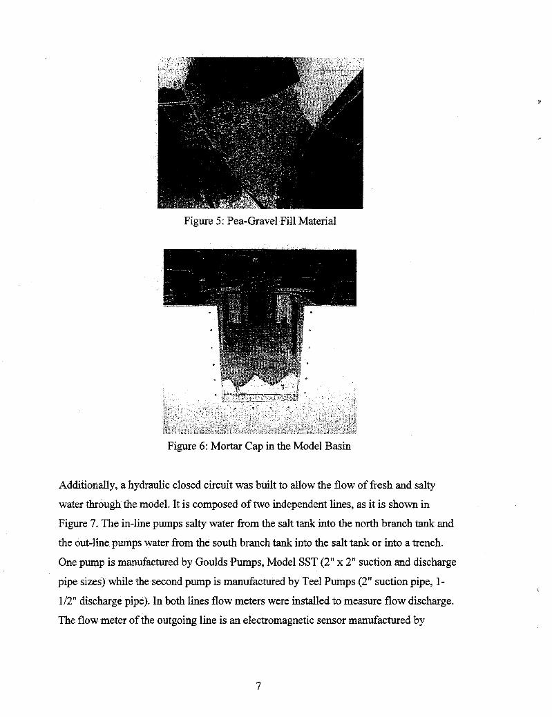
Figure 5: Pea-Gravel Fill Material

Figure 6: Mortar Cap in the Model Basin

Additionally, a hydraulic closed circuit was built to allow the flow of fresh and salty

water through the model. It is composed of two independent lines, as it is shown in

Figure 7. The in-line pumps salty water from the salt tank into the north branch tank and

the out-line pumps water from the south branch tank into the salt tank or into a trench.

One pump is manufactured by Goulds Pumps, Model SST (2" x 2" suction and discharge

pipe sizes) while the second pump is manufactured by Tee1 Pumps (2" suction pipe, 1 - 1/2" discharge pipe). In both lines flow meters were installed to measure flow discharge.

The flow meter of the outgoing line is an electromagnetic sensor manufactured by

UTH /

: 2" PIPE i inside ; 1 trench

TRENCH i 1 i : i

Fig.7: Schematic of the Hydraulic Circuit of the Chicago River Model,

McCrometer Inc. Also, a gate at the exit of the North Branch tank was placed to separate

the incoming flow fiom the water that is stored in the model.

Initial operation of the model revealed the need for additional bracing to maintain the

integrity of the channel walls. Such bracing does not affect the modular construction and

the disassembly and re-assembly of the model.

Model Scaling

In order to maintain similarity between the prototype and model systems for a density-

driven flow, it is necessary to set the ratio of the densimetric Froude number, Fd, or

Richardson number, Ri, between the prototype and model equal to one. The Richardson

number is related to the densimetric Froude number and is defined as:

Where g is the acceleration of gravity, A@ is the excess fractional density, h is the mean

flow depth, and U is the cross-sectional mean velocity.

Keeping the ratio of the Richardson numbers equal to one (Ri, = Rip /Rim, where the

subscripts r, p, and m denote ratio, prototype scale, and model scale, respectively), gives

the following relationship for discharge:

where Qr is the ratio of mean discharges, Wr is the ratio of the horizontal scales, and h, is

the ratio of the vertical scales.

Setting (I/fp;b), - 1/100, W, = 250, and h, = 20 gives a discharge ratio of 2236. Based

upon an ana9ysis of streamgage data collected along the North Branch Chicago River at

Grand Avenue (USGS gage 055361 18, North Branch Chicago River at Grand Avenue),

the average daily flow for the period between November 4,2002 and February 12, 2003

was 260 cubic feet per second (cfs). Using the above factor, the scaled flow rate for the

model. is 0.1 1 6 cfs, or 3.28 liters per second (11s).

Derivation of the Scale Factors

Scaling sf' flow and density gradients was achieved by maintaining the same densirnebric

Froude number, fi, in the model and prototype or the same Richardson number, Ri. n u s ,

the ratio of the Richardson numbers should equal one.

This equation has three degrees of fieedom, Ap,, h,, and Up In order for this equation to

have a unique solution, it is necessary to set two of the parameters, in this case Ap, and

h,. With the fixed geometric scaling used for the model (h, = 250 and W, = 20), there are

two possible approaches to the scaling, detailed below.

First approach - set (Ao/o)

The appropriate waling factors can be obtained by inspection of the Richardson number,

for the case when the excess fractional density in the prototype is set equal to the one in

the model, as follluws:

The discharge, Q, is defined as Q = U x A . Thus,

Q, = U, x A,, where

Therefore, substituting (A2) and (A4) into (A3) gives

Substituting in the values for hr and Wr (h, = 20 and Wr = 250) gives a value of 8, =

22,360. Thus, for a mean daily flow discharge of 260 cfs in the Chicago River, the model

flow would need to be 0.01 16 cfs (0.3 litersls). With a mean model depth and width of

35 centimeters, the mean velocity at this flow rate would be approximately 0.25 c d s , too

small to be measured accurately. Thus, it is necessary to change the excess fiactional

density ratio to get a measurable channel velocity in the physical model.

Second approach - set (Ado), = 1/100

An alternative is to increase the excess fiactional density in the model with respect to the

prototype so that the resulting flow velocities can be measured. This approach yields,

(7) h r 112

Ri, = = I . [ ( j ) ~ ] =U, ur2

Substituting (A6) and (A4) into (A3) gives

Substituting in the values for (Ap/p). h,, and Wr gives a value of Qr = 2,236. The model

flow discharge is therefore 0.1 16 cfs (3 11s) and the mean channel velocity is 2.5 c d s .

These values of flow discharge and mean flow velocity can be accurately measured in the

model with the help of particle-image-velocimetry (PIV) and acoustic Doppler

Velocimeters (AQVs).

Originally, water refrigeration was to be used to produce density gradients. However. an

evaluation of the flow rates needed in the model suggested the need for a fairly large

piece of heat-transfer equipment. The refrigeration units that were available turned out to

be faulty so a decision was made to use an existing tank for mixing of salt and water.

Heat can be lost to the air above the river model, but salt is a conservative contaminant

thus facilitating its control and monitoring in the laboratory. Fine silt and clay particles

will also be used in combination with the salt, so that the fate of solids particles in the

river can be both visualized and studied in detail.

Preliminarv Experiments

In order to test the poteritial occurrence of density currents in the Chicago Ever, a

preliminary experiment was carried out to create a density current in the model and to

measure flow depths and flow velocities. The experimental conditions are given in the

table below.

/ Experimental Conditions for Preliminary Run

Once ttme denser water-salt mixture coming down the North Branch got to the junction

with the Chicago Itiver, it plunged and a density current developed along the bottom,

slowly flowing towards lake Michigan. An acoustic Doppler velocimeter (ADV) was

I

mixture Density of river water

Scale conversion

2236 Discharge

1.01

1.001

Model Prototype 0.116

Temperature 14 Density of water-salt

260 cfs

("C) cfs

used to measure the vertical flow velocity distribution at a river-cross section located at

Columbus Drive. The observed velocity profile was converted to prototype scale and is

plotted in Figure 8 together with observations made by the USGS at the same location.

Even though, the values of flow velocity are not exactly the same, the velocity

distribution in the vertical is quite similar in the model and the prototype. It is important

to keep in mind that the conditions used in the model for this preliminary experiment are

not necessarily the same ones that existed in the Chicago River the day the measurements

where taken by the USGS. Flow discharge is the most reliable parameter but the density

differences that might have been present are more difficult to estimate. However, these

results are encouraging since they clearly point out that density currents are quite likely to

develop in the Chicago River. The model observations also support the trend of the field

measurements obtained by the USGS.

Chicago River Comparison Velocity Profiles at Columbus Drive

---

-5 -4 -3 -2 -1 0 1 2 3

Velocity [cmm)

Figure 8. Comparison of flow velocity distribution observed in the model and in the field.

Future Experimental Work and Analysis of Field Data

While the results obtained so far are promising, it is clear that more experiments are

needed in order to assess the dynamics of density currents in the Chicago River and

the conditions that lead to their development. Field data can be used to compare a id

interpret the experimental observations made so far, and to select future experimental

conditions. Jn particular, a theoretical analysis of the measurements of the event

occurred in March 18, 1998, will serve as guide to determine relevant parmeters

such as plunging point conditions, density differences, flow velocities, discharges,

Bow depths and Richardson number. This analysis is presented below.

From this analysis, it follows that:

In the hydraulic model, the density difference will be best achieved by the

incorporation of salty water. Therefore, a system of inflows and outflou~s of water

having different density (see Figure 7), will be used in the model to maintain the

stable stratification in the system. Series of experiments will be conduded to

determine the range of flow discharges and density differences required to

originate density currents. Also, the temporal evolution of the system will be

studied.

?he equat~ons for prediction of the plunging point and lock exchange show results

that are consistent with the few available field observations. Thus they d l be

applied in the hydraulic model to analyze simple cases, and to compare the

observed values of the location of the plunging point near the junction, a d

average flow depths of the under- and over-flow along the Chicago River.

Further experiments will be carried out to capture the complexity of the bed and

its interaction with the flow to predict the profile of the underflow depth.

Theoretical analysis of field data

The Chicago River presents a very irregular bed, with differences in elevation of the

order of 1 m that is within the order of magnitude of the flow depth (7.3 m). Thus,

depending on the reach the slope could be treated as favorable or adverse to the flow. For

this exercise, the bottom slope was estimated as an average slope with a value of 0.0001.

The mean bottom elevation of the Chicago River slopes down from the junction towards

Lake Michigan. The gradient is very small and different values can be obtained

depending on how it is estimated. However, it is large enough to promote the movement

of denser water coming down the North Branch, towards the lake as a density current.

The flow depth, flow velocities and discharges were obtained by analyzing field

measurements of velocity, conductance and temperature in three cross sections along the

river, taken by the USGS on March 18, 1998. From the junction with the North Branch

going towards the lake these sections are La Salle Bridge, Wabash Bridge and Mc Clurg

Court (Fountain). Figures 9, 10 and 11 show these measurements and Table 1

summarizes the parameters obtained ffom the analysis of the data.

Center Chicaao River at LaSalle Bridge

-0.5 0.0 0.5 1.0 1.5 2.0 2.5 3.0 3.5 4.0 4.5

l -.-m- Temp. ('C) -c Spec. Conduct. (kS/m) --t- Vd. (mlsxl0-1)

Figure 9: Field measurements of temperature, velocity and conductance at La Salle.

-- Center Chicaqo River at Wabash Bridqe

-0.5 0.0 0.5 1.0 1.5 2.0 2.5 3.0 3.5 4.0 4.5

= I

8 1 J

-c- Temp ("C) -a- Spec. Conduct. (kSIm) -Vel (mIsxl0-1) - - - - -

Figure 10: Field measurements of temperature, velocity and conductance at Wabash.

Center Chicaao River at Fountain

-0.5 0.0 0.5 1.0 1.5 2.0 2.5 3.0 3.5 4 0 4 5

i i

1 -Temp. ("C) -Spec. Conduct. (kSlm) +-Vel. (mlsx10-I)

Figure 11: Field measurements of temperature, velocity and conductanc. at Court(Fountain)

If the flow is assumed to be an underflow over a virtual uniform bed located 7.3 m

underneath the free surface, the measurements can be interpreted as follow: the eventual

plunging point could be located upstream of La Salle and the underflow develops fmm

that point towards the lake. The underflow depth is in the order of 2.4 m and the velocity

of the fiont is of the order of -0.03 m / s , which decreases downstream. The latter might

occur due to bottom friction losses. The discharge of the underflow is approximately

equal ti, 0.04 rn3/s/m. Notice that the fi-ee surface of the river can be considered as

horizontal for practical purposes.

The net discharge equals 0.07 m3/s/m, shows that there is a flow fiom the CR into the

South Branch. This flow might be due to water leaking from Lake Michigan, because

these measurements were done before the reparation of the gate locks was completed.

Assuming a value of Ap/p equal to 0.0005, which is in the range of values (0.0001 to

0.001) calculated by Bombardelli and Garcia (2001), the Richardson number is

approximately equal to: 1200 (~~=0.0008) upstream of the plunge point, 83 downstream

of the plunge point and 42 along the underflow and the critical Richardson number is

equal to 5. Also, the entrainment rate is within the range of 10'~ to lo-'. These numbers

indicate that density stratification effects are far more important than inertial terms, thus

entrainment of less dense water fiom above into the underflow can be safely neglected.

Moreover, the slope of the bed is mild, S<Sc=0.007, and the underflow is a subcritical

flow, controlled by downstream conditions. This result indicates that in the physical

model the boundary conditions at both Lake Michigan and the South Branch need to be

set carefully in order to reproduce the behavior observed in the prototype.

Table 1 : Summary of Relevant Parameters.

Densirnetric Froude number (squared) (Aplp=0.0005) Richardson number

Note : Negative velocities indicate flow towards the lake.

0.012 83

0.024 42

0.024 42

Prediction of plunge point conditions

Table 2 shows plunge point depths estimated with the formulas reviewed and values of

coefficients reconmended by Akiyarna and Stefan (1981). Considering that the plunge

point depth should be smaller than 7.3 m and higher than the underflow depth, i.e. 2 3 m,

depending also on the bed elevation, for an average excess fractional density Ap/p equal

to O.OQO5, formulas number 1 and 5 predict reasonable values of this parameter. Also for

lower values of ap/p formulas number 3, and 5 yield acceptable results and for values of

~ p / p closer to 0.001 formulas number 1 and 5 estimate reasonable depths. In addition, in

order to have plunge-point depths of the order of 7.3 m, formulas 1 and 5 yield values of

excess fractional density within the range of the field data.

Table 2: Plunge point depth (hp) and densimetric Froude number (Fp)

qo=0.04 m3lslm.

[ Bottom Slope 0.0001 / 0.0001 1 I Formula NurnberiAuthor I Fp / hp (m) 1 Fp I hp (m) 1 Fp hp (m) apip I 1. Akiyama and Stefan(1984) 1 0.06 1 7.6 1 0.03 1 4.4 / 0.02 1 3.5 1 1E-04 1

Moreover, if a larger flow discharge is considered, for example 0.07m3/s/m, fonnmlas t,3

and 5 yield coherent values of the plunge point depth.

Backwttter profile for the underflow.

Applying the formula for the variation of the underflow depth along the river considering

an internal hydraulics approach (Garcia, 1993) for downstream boundary conditions

between of 0.1 and 2.3 m, the first set arbitrarily and the second is the underflow depth

measured at Fountain, the following profiles were obtained (Figure 12).

Fig. 12 shows that the results are consistent with the expected behavior of the backwater

curve, i.e., the flow depth decreases upstream and the slope of interface decreases as the

downstream depth approaches a depth value of 2.3 m. This behavior is also observed for

higher values of Aplp, with the consideration that the downstream height must be larger

than 1. On the other hand these profiles are only valid within some distance downstream

of the plunging point, where the flow depth varies rapidly. Since there are uncertainties in

the determination of the downstream condition, the reach where these profiles apply, the

determination of the bed slope, and the violation of the assumption that the flow over the

underflow is stagnant and that the thickness of the underflow is much smaller than the

total flow depth, these results should be considered with caution.

Underflow depth along the Chicago River for Ap/p=0.0001

2.5 for different downstream flow depths.

1

0 200 400 600 800 1000 12W 1400 1600 1800 2000

Distance from Lake Michigan (m)

Figure 12: Underflow depth in the Chicago River for Ap/p=0.0001.

Goal of Future Experiments

The main goal of the experiments to be conducted in the next phase of the study will be

to characterize the hydrodynamic conditions that lead to the development of density

currents in the Chicago fiver. Once the phenomenon is well understood, different

alternatives measures (e.g. bottom sill, bubble screen, etc.) that could be implemented to

prevent .the development of density currents will be analyzed in detail with the help crf the

hydraulic model.

References:

Akiyarna, J. and Stefan, H. (1981) Theory of plunging flow into a reservoir.

Internal Memorandum No. IM-97. Saint Anthony Falls Hydraulic Laboratory.

University of Minnesota.

ASCE (2000), Hydraulic Modeling: Concepts and Practice, ASCE Manuals and

Reports on Engineering Practice No 97, Reston, Virginia, 390p.

Bombardelli F. and Garcia, M.(2001) Three-dimensional hydraulic modeling of

density currents in the Chicago River, Illinois". Civil Engineering Studies, Hydraulic

Engineering Series N-68, Ven Te Chow Hydrosystems Laboratory, department of

Civil and Environmental Engineering. UIUC, Illinois.

Garcia, M.H. (1993), "Hydraulic Jumps in Sediment-Laden Bottom Currents,"

Journal of Hydraulic Research, American Society of Civil Engineers, 199: 1094-1 1 17.

Garcia, M.H. (1 994), "Depositional Turbidity Currents Laden with Poorly-Sorted

Sediment," Journal of Hydraulic Engineering, American Society of Civil Engineers,

120: 1240- 1263. (Received the 1996 Karl Emil HiIgard Prize for best publication in

the Journal of Hydraulic Engineering)

Nino, Y and Garcia M. CEE 498 Environmental Hydrodynamics, Department of

Civil and Environmental Engineering, UIUC, Urbana, Illinois, Spring 2003.