research and development expenditures and labor … · chapter title: research and development...

This PDF is a selection from an out-of-print volume from the National Bureau of Economic Research

Volume Title: New Developments in Productivity Measurement

Volume Author/Editor: John W. Kendrick and Beatrice N. Vaccara, eds.

Volume Publisher: University of Chicago Press

Volume ISBN: 0-226-43080-4

Volume URL: http://www.nber.org/books/kend80-1

Publication Date: 1980

Chapter Title: Research and Development Expenditures and Labor Productivity at the Firm Level: A Dynamic Model

Chapter Author: M. Ishaq Nadiri, George C. Bitros

Chapter URL: http://www.nber.org/chapters/c3918

Chapter pages in book: (p. 387 - 418)

7 Research and DevelopmentExpenditures and LaborProductivity at the FirmLevel: A Dynamic ModelM. Ishaq Nadiri and George C. Bitros

7.1 Introduction

The importance of innovative activities to the development andgrowth of the aggregate economies, various industries, and finns hasbeen clearly established (see Kamien and Schwartz 1975). Issues suchas the determinants of R and D expenditure, the rate and process ofdissemination of innovative activities, the rates of return on R and Dinvestment, the role of uncertainty in the undertaking of these efforts,and finally the industrial and organizational aspects of innovative activi-ties have been the subject of numerous investigations.' Though there isconsiderable uncertainty about the quantitative evidence, the importanceof research and development efforts in increasing productivity and de-veloping new products has been generally accepted. However, one issuethat has not received sufficient attention is the integration of the demandfor research and development expenditure of the firm with its demandfor conventional inputs such as labor and physical capital. The need forsuch undertakings is clear; R and D, like expenditure on plant andequipment and labor, is an input to the production process and there-fore an integral part of the overall decision framework of the firm.

The primary purpose of this study is to investigate the determinantsof research and development expenditure in the context of a general

M. Ishaq Nadiri is at New York University and the National Bureau of Eco-nomic Research. George C. Bitros is with the Bank of Greece.

The research for this paper was supported by the National Science Foundation(SOC 74—16295). We are indebted to Shoshona Livnat and Susan Chen for theirdiligent assistance in assembling the data and computation of the results.

1. Some examples of such studiesare Baily (1972), Grabowski (1968), Kamienand Schwartz (1974, 1975), Mansfield (1968), Mansfield et a!. (1971), andScherer (1965).

387

-F

388 M. Ishaq Nadiri/George C. Bitros

dynamic model of a set of input demand functions. The consequencesof research and development for other inputs and the impact of changesin demand for labor and physical capital on R and D decisions aretreated together using a disequilibrium adjustment model of input de-mands. Within the context of this model the following issues are ana-lyzed: (a) the short-run effects of changes in output and relative priceson demand for innovative activities, measured by stocks of R and Dexpenditure, employment, and capital stock; (b) the effects of the excessdemand in any of these inputs on the short-run demand for the otherinputs; (c) the effects of research and development and plant andequipment expenditures on labor productivity in the short, intermediate,and long runs; and (d) the responses of the inputs of firms of differentasset sizes to changes in relative prices and output changes and thepattern of interactions among their inputs over time.

The main results of this study can be summarized briefly:1. Changes in output and relative input prices significantly affect, in

the short and long runs, the firm's demand for labor, research and de-velopment activity, and capital goods.

2. The transitory or distributed lag responses of the inputs to changesin output and relative prices are interdependent, i.e., a dynamic andasymmetrical feedback system is operative among the input responseswhich traces the adjustment of the system of input demands toward itslong-run equilibrium.

3. Substantial differences exist among the cross-section of firms intheir employment, research and development activity, and physical capi-tal accumulation. Also, there is evidence of systematic overtime differ-ences in their demand for labor, research and development activities,and capital goods.

4. Research and development investment exerts significant influenceon the short and long-run behavior of labor productivity.

5. Finally, no discernible differences in input demand functions werefound when firms in our sample were classified by the size of their assets.

The plan of the study is as follows: The rationale of the disequilib-rium approach to the analysis of input demands is described in Section7.2. An example to illustrate the issues is provided and the outlines ofthe structure of the model are stated in this section. In section 7.3, theestimating equations, the characteristics of the data, and some estimationproblems are described. The structural estimates Of the model usingdata for sixty-two firms for the period 1965 to 1972 are presented anddiscussed in section 7.4.1. In Section 7.4.2 the structural estimates ofthe model fitted to samples of firms classified by their asset sizes arepresented. The stability of the model is also examined. In section 7.5,the cross-sectional differences among firms in their demand for inputsare noted and the overtime differences among input demands are ana-

- t

389 Research and Development Expenditures

lyzed. Furthermore, the long-run output and price elasticities of em-ployment, research and development, and capital stock are discussedin this section. Also, the short, intermediate, and long-run effects ofresearch and development on labor productivity are examined. Thesummary and conclusions are stated in section 7.6, followed by anappendix where the sources of data, construction of the regression vari-ables, and the names and classification of the firms by the size of theirassets are reported.

7.2 The Rationale for a Dynamic Disequilibrium Model

Existing cross-section and time series models of the determinants ofR and D behavior assume fixed stocks of capital and labor. Also, noallowance is made in the employment and investment literature for thefact that a firm's R and D activities will affect its cost structure and thusits demand for labor and capital. That is, decisions with respect to theconventional inputs will be influenced depending on when and howvigorously the firm engages in innovative activities. In turn, a firm'sdemand for research and development effort will be affected by themagnitudes and characteristics of its capital and labor. In this type ofinteractive process, all the inputs are essentially variable and are onlydifferentiated from each other by the degree of their flexibility or adjust-ment over time.

The dynamic model described below permits interaction among theseinputs over time. The main feature of the model is that the disequilib-rium in any of the inputs has a spill-over effect on demand for otherinputs in the short run, while in the long run all excess demands disap-pear and the spill-over effects vanish.2 However, in the very short run,as the firm attempts to adjust its stocks of inputs it will increase theutilization of its existing stocks to meet current demand. As the stockadjusts, the utilization rates return to their optimum levels.

7.2.1 An ExampleTo illustrate the nature of dynamic interactions among time paths of

inputs, consider a simple two-factor example. Suppose the productionfunction is x = f(yi, Y2), where x is output, Yt and Y2 are inputs, and fhas the usual continuity properties. Two isoquants are illustrated infigure 7.1. The dotted line AB is the locus expansion points

2. We recognize that the dynamic input and output paths are jointly deter-mined, contingent on future product price expectations. But their joint estimationrequires a full market theory not yet available. Therefore, we set the limited goalof estimating optimum input paths consistent with an optimum and given outputpath. This allows us to concentrate on interactions among changes and on factorsubstitution.

390 M. Lshaq Nadiri/George C. Bifros

x2

y1

Interactions among Time Paths of Inputs

along which total costs are minimized and is derived in the conventionalway. Though this may be an adequate description of long-run behavior,there is plenty of evidence to suggest that firms do not remain along ARat every moment, and several explanations for this divergence havebeen offered. Most important, in addition to direct rental charges offactors, there are costs involved in changing their levels; that is, thereare substantial transactions costs, and these must be viewed as additionalinvestment costs if they are to be undertaken. There are search, hiring,training, and layoff costs and associated morale problems among work-ers. Similarly, there are searching, waiting, and installation costs inpurchasing new capital goods, and there are adjustment costs associatedwith changing the level of the R and D activities such as acquisition ofthe appropriate facilities, search cost in hiring and training of scientistsand engineers, etc. If initial input values deviate from their long-runequilibrium levels, existence of these costs implies that optimum adjust-ment paths to equilibrium are not instantaneous. Since exogenous vari-ables are generally subject to change and uncertainty, these costs oftenmake it profitable for firms to engage in hoarding of input stocks.

The conventional way of incorporating adjustment costs is the well-known partial adjustment model:

(1) yit—yit_i=$(yit-—yie_i), Q</3<1,where is the desired level of as defined by AB and p is the adjust-ment coefficient. Suppose the firm wants to increase output to x2, giveninitial condition A in figure 7.1. Equation (1) implies an immediatemove from A to (say) C, with convergence along the new isoquant tothe new equilibrium point B. The diagram indicates a correspondingand implied adjustment path for In general, two independent ad-

Fig. 7.1


justments imply additional hypotheses concerning the role of the pro-duction function during the adjustment period. There are two possibil-ities:

i) If the production function constraint always holds as an equality,independent adjustments imply an output decision function, which maynot be optimum.

ii) If output is taken as exogenous, two independent specificationsmean that firms must be off their production functions, i.e., they mustbe capable of producing more than they actually do during the adjust-ment period.4

An intermediate position is also possible—that is, to assume outputto be exogenous, but input adjustments are specified to be interrelated.For example, a generalization of equation (1) is

(2) [Yit — Yit—i 1 = /3121 [Y2t — Y2t—1

LY2t — Y2t—1 J Lfl21 /322 J — Yit—i

This incorporates exogenous output and allows firms to remain on theirproduction functions during the adjustment process, since input adjust-ments are not independent.5 Refer again to figure 7.1. If the true adjust-ment path is described by ACB, $21 and /322 must be sufficiently positiveto initially push y2 above its ultimate value. This overshooting sets upforces that ultimately decrease Y2 to its equilibrium value at B. The netvalues of and/312 must be positive for Ys to increase monotonicallyto its equilibrium at B. Obviously, there must be restrictions on theto insure that the firm remains along isoquant x2x2.

7.2.2 The Model of the Input Demand FunctionsAssume that the firm minimizes costs subject to a Cobb-Douglas

production function with three inputs: labor (L), capital stock (K),and stock of research and development activities (R). The input and

3. Assume f is Cobb-Douglas, x = (y1)a(y2)b. The demand for y2 may be de-rived from a logarithmic form of equation (1) and from y2 = (x)h/b(y1)—0/b.It is given by

Y2t = (Yit—i)—a/b

4. Nerlove (1967). Nerlove adopts the second approach. In his model, firmsreact not to observed values of output and relative prices, but to forecasts ofunobserved (trend.cycle) components. Desired and actual output are identical,but firms may be off their production functions.

S. It is interesting to note that a similar hypothesis has been proposed byBrainard and Tobin (1968) in the related context of portfolio adjustment amongassets. These authors have assumed the wealth path to be exogenous and haveaddressed themselves to determining optimum adjustments of various assets con-sistent with that path.


output prices are assumed to be exogenously given. More formally, thegeneral problem considered is to minimize costs,

(3) C=wL+cK+rRsubject to the production function

(4) Q = Ka2 Ra3 Ua4

where w, c, and r are respectively the user costs associated with em-ployment, stock of plant and equipment, and stock of research anddevelopment. Q is the level of output, A is a constant, a1, a2, and a3are the long-run output elasticities of the inputs, and A is the rate ofdisembodied technical change. We have assumed that the input utiliza-tion rates are functions of an overall rate of utilization, U. Also notethat the utilization rate U does not explicitly enter the cost function,but implicitly through the rate of depreciation, 8, of capital stock. De-preciation depends on the rate of utilization, U, as well as time, i.e., S= S(U,t).

The user costs are defined to include the purchase price, the oppor-tunity costs of funds, depreciation expenses due to utilization and pas-sage of time, tax considerations, and capital gains. For example, theuser costs of capital goods can be stated as

P1 is the deflator for capital goods; r is the cost of capital, mea-sured as r = i — (P/P)8, where i is long-term interest rate and (p/P)eis the expected change in prices; S is the depreciation rate; P and P arethe level and change in general price level; k is the Long tax creditamendment; k' is the effective rate of tax credit; z is the present valueof depreciation; and v is the corporate tax rate. The user costs for laborservices and for research and development efforts are in principle simi-lar to c. The Langrangian method for minimizing costs (3) subject tothe production function (4) will yield the long-run solution of thedeterminants of the inputs.6 That is,

= L = gj(x*, F)y2—R—g2(x'P)

(5) y*3_K_gs(x*P)= U =

where P is a vector of the relative prices of inputs and the coefficientof xs is i/p = (aj + a2 + a3), the reciprocal of returns-to-scale pa-

6. See Nadiri and Rosen (1973), pp. 19—21, for derivation of these expressions.

T393 Research and Development Expenditures

rameter. Assuming that the adjustment cost of each input is proportionalto the gap between its long-run equilibrium and actual levels and is alsoaffected by the disequilibrium of the other inputs, it can be shown thatthe approach to the long-run equilibrium of the system of inputs isapproximated by the following set of difference equations (Nadiri andRosen, 1973, pp. 24—25).

4

(6) Yit — Yit—i = — y,t] + V4t,1=1

(i=1, . . . , 4),

where is a nondiagonal matrix of adjustment coefficients and v1,v4 are random terms with zero means and variance-coverance

matrix if From the generalized adjustment model (6) we can find(a) the short-term impact of changes in output and relative input prices,(b) the transition or distributed lag patterns of the inputs to a changein these variables, and (c) the long-run price and output elasticities ofthe inputs. Since the technical details of these problems are discussedelsewhere (Nadiri and Rosen 1969), we may state that the short-termtransitory responses are calculated by computing [I — (1 B) Z]'and the long-run elasticities by calculating A[1 — B]—'; B = is thenondiagonal matrix of adjustment coefficients, Z is the lag operator, andA is the matrix of the coefficients of the exogenous variables.

7.3 Estimating Equations: Data and Estimation Problems

The model specified in section 7.2 has been estimated using cross-section and time series data on sixty-two firms for the period 1965—72.The main source of our firm data is the Compustat tapes. The sixty-twofirms are drawn from five industries: five from Metal extraction (SIC10), twenty-eight from Chemicals and allied products (SIC 28), twelvefrom Nonelectrical machinery (SIC 35), eight from Electrical equip-ment and supplies (SIC 36), and nine from instruments (SIC 38).Thus, our sample is dominated by firms in the Chemical and alliedproducts categories.

The empirical specification of the model differs somewhat from (6).The user costs of labor and research and development efforts have beenomitted due to lack of appropriate data. The real wage rates for theappropriate two-digit industries are used as a proxy for these two user-cost variables. The user cost of capital for each firm is approximated bya measure constructed for the total manufacturing sector.7 The outputprices are not available at the firm level; therefore, we have used appro-

7. See the appendix for the specific formulation and source of data to generatethis variable.

-J

394 M. Lshaq Nadui/ George C. Bitros

priate wholesale price indices of the two-digit manufacturing industriesas the deflators for output, nominal wage rate, and the user cost ofcapital.

The proper concept for the research and development is the servicesof a given stock of R and D to the production of current output. Reli-able estimates of the benchmark and depreciation rates for R and D atthe individual firm level are not available. We constructed the stock ofR and D by assuming an arbitrary depreciation rate of 10% per annumfor each firm. The 1965 R and D investment in constant dollars is usedas the benchmark for those firms that did not report any figures priorto 1965, while for firms with more extended data, the first year of con-sistent reporting was chosen as the benchmark.8 Capital stock series forR and D and plant and equipment for each firm were constructed bythe recursive formula,

(7) = + (1 — (i = 1, . . . ,62),

where is the deflated individual firm expenditure on R and D or newplant and equipment; the deflator used for converting nominal expendi-ture on R and D and plant and equipment into constant dollars is thedeflator for plant and equipment (1958 = 100). The &, are the indi-vidual firm depreciation rates calculated for plant or equipment as theratio of depreciation expenses to the benchmark capital stock obtainedfrom the firm's balance sheet. As noted earlier, the depreciation ratesfor R and D are assumed to be fixed at 10%. The employment datarefer to total employment of each firm. Unfortunately, it is not possibleto break this aggregate series into production and nonproduction orscientists and engineers, etc. Similarly, it is not possible to separate theresearch and development expenditure into privately and publicly fi-nanced categories.

The specific estimating equations used are

= a0 + aiQt + aa(w/c)t + ++ + + Ei,

= /3o + + 132( W/C)t + + f34Rg_1

(8) + + += Yo + + ya(w/c)t + +

+ + += + 8iQt + + + 84Rt_1

+ + +8. The regressions were also run with the flow measure of R and D expenditure.

The overall results were generally similar to those reported in table 7.1.

J


where all the variables are in logarithms; is the measure of researchand development expenditures; and are the levels of employmentand capital stock of the firm; Qt is the level of output; (Wt/Ct) is theratio of nominal wage rate and the user cost of capital goods. Ut isthe rate of utilization of the appropriate two-digit industries used as aproxy for firms' utilization rate, R1_1, and are the laggeddependent variables, and €3, and are the error terms.9

The adjustment processes are embedded in the coefficients of thelagged dependent variables. The own adjustment coefficient in eachequation can be obtained from the regression coefficient associated withthe lagged dependent variable, while the cross-adjustment coefficientsare from the regression coefficients related to the lagged values of otherdependent variables. For example, in the first equation of (8), the ownadjustment coefficient is flu = (1 — a3) and the cross-adjustment ef-fects of disequilibria in R and D and plant and equipment on employ-ment are measured by —/312 = a4 and —/313 = a5. The matrix

r a3 a4 a5 a6

I Y3 Y4 Y5 Y684 85 86

constitutes the 4 X 4 nondiagonal adjustment matrix which traces theinterdependence of the adjustment paths of the three inputs and theutilization rate over time.

Before estimating these equations, the problem of heteroscedasticityin our sample had to be considered. Except for the three aggregateindustry-wide variables wt, Ct, and the remaining variables in (8)are specific to each firm. Error variances for large firms will substantiallyexceed those of small firms and therefore the possibility that the cross-section within-cell regression functions will have unequal error varianceswill exist. As is well known, there are two ways to handle this possi-bility; the first is to test for the existence of heteroscedasticity amongfirms and eliminate the statistically significant outliers. The second ap-proach is to transform variables so that the error variances will behomogenous (Kuh 1963). We have followed the second alternative.Two possibilities exist: (1) log transformation of the variables whichequalizes the error variances on the assumption that they are strictlyproportional to the size of the independent variables; (2) fitting themodel in ratio form, which means dividing the firm-specific variablesby an appropriate scale variable such as the total assets of the firm.Though we have used both of these procedures (using total deflated

9. See the appendix for definition, sources, and construction of the regressionvariables.

396 M. Ishaq Nadiri/ George C. Bitros

assets of the firms as the denominator in the ratio form of the model),we shall report only the logarithmic results.

Another important estimation problem that arises immediately iswhether or not to impose the implicit constraint on the adjustmentcoefficients of model (8). If the adjustment coefficients are uncon-strained, one of two hypotheses about the production function is im-plied: (1) if the production function constraint always holds as anequality, then the adjustment process implies that output is endogenousduring the adjustment period; (2) on the other hand, if output is takenas exogenous, independent adjustments imply that firms may not be ontheir production functions. The values of the adjustment coefficients,then, will determine whether the firms are inside or outside of theirproduction surface.

We have not imposed the necessary constraints on the adjustmentcoefficients, mainly because of the unreliability of the underlying data.Instead, we have assumed that output is endogeneous and have exam-ined the unconstrained estimates of the adjustment coefficients to seewhether the constraints implied by the model are met. The structuralequation for each input is estimated by two-stage least-squares and thecharacteristic roots of matrix B are examined to check whether the im-plicit constraints are reasonably met.

7.4 The Structural Estimates

The model is estimated using the variance components technique forpooling cross-section and time series data developed by G. S. Maddala(1971). This method allows estimating the cross-section and time serieseffects separately and generates generalized least-squares estimates ofthe parameters of the model.'°

The model (8) is estimated using the overall sample of sixty-twofirms and three subsamples: twenty-eight firms with total assets below$300 million, twenty firms with assets greater than $300 million butsmaller than one billion dollars, and fourteen firms of over one billiondollars in total assets. The estimation of the model using the stratifiedsamples should provide a test of its stability and insight into whetherfirms of different sizes differ in their input decisions. We have also esti-mated both the ratio and logarithmic forms of (8) for all four samples.Only the generalized least-squares estimates of the model in logarithmicform are presented here.

10. The computer program based on this technique generates four regressions:the ordinary least squares (OLS), generalized least squares (GLS) without takingeffect of cross-section and time effects, the least squares plus dummy variables(LSDV), which takes account of these effects, and finally the generalized leastsquares with dummy variables.

I


7.4.1 The Structural Estimates: The Overall SampleThe results in table 7.1 are the generalized least-squares estimates

with cross-section and time dummies. Note that Qt is the estimated valueof the output variable

The results indicate a consistent picture: the coefficients generallyare statistically significant in both the OLS and GLS versions, the resultsof the ratio and logarithmic forms of the model were fairly similar, andthe signs of the coefficients of all the variables except a few remainedstable in the various versions of the model.

As can be seen from table 7.1, the statistical goodness of fit of themodel measured by R2 and sum of squared residuals (SSR) and esti-mated variance of errors (EEV) are very good. A separate test usingthe TSP regression program indicated that the Durbin-Watson test valueswere about 2.0 for each of the equations. However, this test is not onlybiased when a lagged dependent variable is included as an explanatory

Table 7.1 Generalized Least-Squares Estimates of the Model inLogarithmic Form, Period 1965—72

Generalized Least-Squares

IndependentVariables

Equations

Log Log Log Log

Constant —.3458(—.5135)

.6793 —.3035(1.889) (—.8140)

—.2013(—2.077)

Log Q .3355(5.482)

.1970 .2279(7.614) (5.758)

.0290(2.933)

Log —.1742

(—1.6855)

—.2418 .0254

(—1.876) (.1773)

.0300

(.8151)

Log .5173(8.507)

—.0904 —.0353

(—3.422) (—.9482)

—.0253

(—2.745)

Log .0997

(2.75)

.6999 —.0046

(42.40) (—.2094)

.0074

(1.34)

Log —.0544(—1.62)

.0804 .8175

(5.391) (40.33)

—.0099

(—1.95)

Log —.3859

(—2.220)

—.1772 —.4388

(—2.52) (—3.565)

.6504

(20.42)

R2 .9283 .9767 .9878 .8851

SSR .3469 .3531 .3475 .3353

Degrees of freedom 365 365 365 365

EEV .0105 .0017 .0054 .00033

Noic: Abbreviations are explained in the text.


variable, but also may not be invariant with respect to the ordering ofthe firm data in our sample.

The estimates in table 7.1 indicate the immediate responses of theinputs to changes in output, relative input prices, their own lags, andcross-adjustment effects of other inputs. The coefficient of output ispositive and statistically significant in each equation. The output elas-ticities indicate that changes in output have the strongest effect onemployment (.34), followed by stocks of capital goods and researchand development. The output elasticity of the utilization rate, U, whichshould be very high, is rather small. The explanation for this is that ourmeasure of the utilization rate is an industry measure which may notrespond greatly to movements of demand of the individual firms. Therelative price variable is also statistically significant and negative inboth research and development and employment equations; it has thecorrect positive sign but is not statistically significant in the capital stockequation or in the utilization equation.

The own lag coefficients of the three stock variables indicate thatemployment adjusts very rapidly (1 — .52 = .48), followed by stockof research and development expenditures, (1 — .70 .30), while cap-ital stock adjusts very slowly (1 — .82 .18). These patterns of ad-justment are consistent with our a priori notion and previous results.They suggest, if we ignore the spill-over effects, an average lag of a yearfor employment, two and one-half years for research and development,and about four years for the capital stock.1' The adjustment coefficientfor the utilization rate is unexpectedly long. Again, part of the reasonis that U is an industry measure and cannot be explained readily bymovements of firm data. There are significant cross-adjustment effectsin each demand equation, though of varying magnitudes. These arecalculated as —fL,, i j—that is, the negative of the cross-adjustmentcoefficients shown in table 7.1. For example, j = 2,3,4 measuresthe effects of excess demand in employment on stocks of research anddevelopment and capital and the utilization rate; they are shown by thecoefficients in row in table 7.1. The signs and magnitudes of thecross-adjustment coefficients vary among the equations, indicating anasymmetrical and varying disequilibrium effect. As noted, the directionof these effects will be the opposite of the signs of the coefficients shownin table 7.1.

1. Employment disequilibrium has strong positive effects on the utili-zation rate and stock of research and development expenditure. It alsoaffects demand for capital goods positively, but the effect is not statis-tically significant. Thus, excess demand for labor increases the utilizationrate and demand for plant and equipment and research development.

11. These calculations are only very tentative, for the adjustment patterns areinterdependent and they cannot be ignored.

c.


2. Excess demand in stocks of research and development has a strongnegative effect on demand for labor; its impact on capital stock is posi-tive but not very significant; its effect on the utilization rate, thoughpositive, is barely significant statistically. Thus, disequilibrium in R andD capital reduces demand for labor but increases that of physical capi-tal, implying a complementary relation with labor and a substitutionalrelation with physical capital.

3. Disequilibrium in physical capital has statistically significant posi-tive effects on demand for labor and the utilization rate while it has astrong negative and statistically significant impact on demand for re-search and development expenditures. These patterns of response suggesta short-run complementary relation between stocks of capital goods andresearch and development and a substitutional relation with employ-ment.

4. The cross effect of the rate of utilization on the demand for em-ployment, research and development, and capital goods is positive andstatistically significant in all cases. That is, disequilibrium in the utiliza-tion rate leads to increased demand for productive inputs.

5. These disequilibrium effects suggest that a firm faces excess de-mand in one of its inputs by increasing its rate of utilization and ad-justing its demand for other two inputs. Thus, strong feedbacks anddynamical relations exist among the inputs in the short run.

From these results we conclude that there are strong and statisticallysignificant short-term effects of changes in output and input prices onresearch development, employment, and investment demand of the firm.Also, there are some lags in achieving the desired levels of these inputs.The lags arise not only because of factors generating disequilibria in thespecific input's own market but also because of disequilibria in otherinputs as well. Dynamic feedback or spill-over effects among the threeinputs do exist, and they tend to be asymmetrical in character. Theutilization rate serves as a buffer allowing the firm to change its stocksof input. That is, when current demand increases, firms utilize theirexisting stocks of inputs first and then, if the demand is perceived asmore permanent, they will adjust their stocks of inputs.

7.4.2 Structural Estimates for the SubsamplesThe results in table 7.1 are essentially repeated when the model is

fitted to the three subsamples mentioned earlier. The structural esti-mates for the subsamples are presented in table 7.2. The striking overallconclusion that emerges from a comparison of the results in tables 7.1and 7.2 is the stability of the model in terms of signs and significanceof the coefficients, and the goodness-of-fit statistics such as R2 and sum-of-squares errors. The magnitudes and statistical significance of thecoefficients vary somewhat across different asset sizes. The output van-

I

Tabl

e 7.

2G

ener

aliz

ed L

ast-S

quar

es E

stim

ates

of t

he M

odel

in L

ogar

ithm

ic F

orm

for T

hree

Sam

ples

of F

inns

, Per

iod

1965

—72

Inde

pend

ent

Var

iabl

es

Twen

ty-E

igbt

Sm

all F

irms

Equa

tions

Twen

ty M

ediu

m-S

ized

Firm

Equa

tions

sFo

urte

en L

arge

Firm

sEq

uatio

nsLo

gL,

LogR

,Lo

gK,

Log

U,

LogL

,Lo

gR,

LogK

,Lo

g U

,Lo

gL,

LogR

,Lo

gK,

Log

U,

Constant

— .0

175

(—

.019

8).8677

—.4

155

(1.8

88)

(—

.736

1)—

.179

5(—

1.51

8)—

3.41

75(—

2.03

1).1

419

.351

7(.4

093)

(.5351)

— .3

415

(—1.

432)

.669

0(.4

639)

.091

7.7

089

(.192

1)(1.059)

— .0

591

(—.1

638)

LogQ,

.1828

(2.003)

.2093

.2459

(5.7

55)

(3.4

08)

.0231

(1.725)

.564

0(5

.274

).1072

.1977

(2.424)

(3.821)

.0341

(1.745)

.9619

(5.692)

.0913

.2290

(1.9345)

(3.7395)

.0428

(1,1480)

Log(w/c),

— .1

410

(—

.425

4)—

.321

6.0615

(—1.

975)

(.2779)

.0319

(.6954)

.6427

(1.187)

— .0

057

—.0

190

(—.0

396)

(—

.082

1).0

797

(.950

6)—

.636

7(—1.285)

.0718

—.0

990

(.4457) (—

.441

0).0024

(.0185)

LogL

,1.6587

(7.309)

— .1

394

—.0

324

(—3.7)

(—.4

831)

— .0

175

(—1.3793)

.1329

(1.015)

.0038

—.0

342

(.0832) (—

.552

5—

.033

1(—1.571)

.1581

(1.417)

—.0241

—.0

589

(—.7772) (—1.4703)

— .0

333

(—1.3625)

LogR,

.102

8(2

.162

5).6

569

—.0

164

(32.981)

(—

.472

).0042

(.6090)

.434

7(3

.778

4).9

365

.076

8(3

5.53

2)(1

.605

).0

157

(1.1

005)

— .0

386

(—.4

965)

.783

5—

.010

1(3

4.78

7)(—

.342

8).0

141

(.791

3)

LogK,.1

— .0

649

(—1.

516)

.107

9.7

994

(6.2

154)

(24.609)

— .0

114

(—1.8116)

— .2

485

(—1.2013)

— .0

801

.6827

(—2.831)

(15.182)

— .0

185

(—1.1888)

— .3

430

(—3.0043)

.0596

.7417

(1.6578)

(15.172)

— .0

350

(—1.4667)

Log

U,_

1—

.304

9(—1.0693)

— .1

769

—.5

847

(—1.683)

(—2.466)

.6607

(13.85)

— .3

088

(—1.2013)

— .1

775

—.1

429

(—1.

481)

(—1.1042)

.627

2(1

0.98

8)—

1.30

89(—

3.92

2)—

.242

1—

.446

9(—

2.53

4)(—3.546)

.626

5(8

.323

2)

.964

8.9923

.9897

.9443

.9632

.9968

.9835

.9668

.7802

.9798

.9515

.7675

SSR

.156

2.1

608

.156

8.1

537

.109

9.1

062

.107

9.1

037

.076

04.0

7927

.076

72.0

7610

Deg

rees

of

free

dom

161

161

161

161

113

113

113

.

113

7777

7777

EEV

.013

4.0

018

.010

5.0

003

.005

2.0

014

.001

3.0

002

.007

8.0

006

.000

9.0

004


able is statistically significant in all of the regressions; the magnitudesof the coefficients are larger and similar to that of the overall samplefor the firms with assets greater than one billion and those with assetsless than 300 million dollars. For the "medium" size firms the short-term responses of the inputs to changes in output, except in the employ-ment equation, is somewhat smaller. The relative price variable (w/c)has the correct sign in most cases, but in most of the regressions itsmagnitude and statistical significance varies. However, except in theemployment equations, the coefficients of the relative price variable arestatistically insignificant.

The own and cross-adjustment coefficients are quite strong in someof the regression equations in table 7.2. The asymmetrical pattern notedfor the whole sample holds in the subsample regressions as well; themagnitudes of the own and cross-adjustment coefficients, however, varyamong firms with different asset sizes. The weakest links in the feedbackamong the input disequilibria are observed in the effects of excess de-mand for R and D of firms with assets over one billion dollars. Dis-equilibrium in capital stock has strong effects on the demand for researchand development of firms in all asset categories. The utilization ratepositively affects the demand for all the inputs as we noted earlier forthe whole sample of firms. The employment disequilibrium has a fairlyweak effect on demand for R and D and capital stock in the medium-size and large firms.

Though these differences in individual coefficients may exist, still theoverall significance of these differences may not be very significant. Totest the stability of the model across the asset classifications, we com-puted the relevant F statistics for each set of input demand equations,

F — SSRT — (SSR14 + SSR20 + SSR28)/k— (SSR14 + SSR20 + SSR28)/N—3k

where is the sum-of-squared residuals from the regression for the62 firms and SSR14, SSR20, are the sum-of-squared residualsfrom the regressions for the subsamples of firms. N is the overall num-ber of observations and k is the number of the parameters estimated.The calculated F statistics for L, R, and K equations are 0.689, 0.9504,0.8927 and 0.2652, respectively, and the critical value of F(7,344) atthe 1 % level is 2.69. Therefore, the null hypothesis of an unchangingstructure of demand functions for labor, research and development, andcapital goods cannot be rejected.

The Cross Section and Overtime Differences among FirmsThe analysis of variance employed in estimating the demand equa-

tions permits testing whether cross-section and time series differencesexist among our sample of firms in their input decisions. We have calcu-

]


lated the F statistics based on the estimates generated by the least-squares plus dummy variables (LSDV) of the analysis of variance. Theresults in table 7.3 pertain to the logarithmic form of the model usingthe entire sample and the three subsamples of firms. They indicate aninteresting pattern: substantial cross-sectional differences exist amongfirms with respect to all of the inputs and, except for the demand forresearch and development expenditure in the small and medium-sizefirms, all the input functions also vary over the span of time considered.

It is difficult to precisely state the causes of the cross-sectional andtime series differences among the samples of firms in their input deci-sions. The cross-sectional difference may arise from the differences inthe characteristics of firms such as being in different industries, produc-ing different types of products, having different degrees of monopolyor monopsony in the markets, etc. The overtime differences may be dueto differing adjustment processes, responses to external shocks, andtechnological changes. Though very desirable, a closer look into the

Group

Effects

DependentVariable Cross Section Time-Series

Overall sample: sixty-two firms 63.5776245.08721.671219.5848

5.209610.30057.6988

173.861

Fourteen large firms 81.5190161.635204.78045.4924

3.52419.2359

18.03093 1.5152

Twenty medium-sized firms

.

48 1.67538.3298

267.81147.5290

62.94521.16499.7051

90.3784Twenty-eight small firms 357.410

321.93214.564316.1273

41.11403.63812.5744

90.8643

NOTE: The critical values of F for the cross-section estimates at .05 are approx-imately as follows: F(61,305) 1.47 for the entire sample, F(13,65) = 2.42 forthe fourteen large firms, F(l9,95) = 2.09 for the medium-sized firms, F(27,135)= 1.85 for the twenty-eight small firms. The critical values of F for the time seriesestimates at .05 are respectively F(5,305) = 3.09, F(5,65) = 3.29, F(5,95 =3.20, and F(5,135) = 3.17.

I

Table 7.3 Values of F-Statistics from Analysis of Variance for the EntireSample and Three Subsamples of Firms, Period 1965—72


sources of these differences in input demand functions of the firms isbeyond the scope of our present research.

7.5 The Long-Run Elasticities of Inputs and Labor Productivities

From the structural estimates reported in tables 7.1 and 7.2, we cancalculate the implied long-run output and price elasticities of the threeinputs. Using these statistics, it is possible to obtain the long-run laborproductivity estimates for the total number of firms and for the sampleof firms classified by asset size. The long-run elasticities are identicalto the coefficients of equation (5) (in log form) and are computedfrom the stationary solutions of the structural equations (8). Note thatthe long-run output elasticities of employment, research and develop-ment, and capital stock demand functions estimate the inverse of re-turns to scale, i/p = 1/(a1 + a2 + a3).

Several features of these figures in table 7.4 should be noted:1. The surprising similarity of the output elasticities among the in-

puts. Long-run elasticities of capital, however, tend to be somewhatlarger in the overall sample and the sample of small firms.

Table 7.4 Long-Run Output and Price Elasticities for theOverall Sample and Subsamples of Firms

Sample Size

Variables

Output Relative Prices

Sixty-two firmsL .7103 —.5954R .7142 —.6946K 1.0521 .0029U .0172 .1143

Fourteen large firmsL .8495 —.7816R .5212 .1656K .6822 —.4230U —.0056 .1222

Twenty medium-sized firmsL .8365 — .6632R .7922 —.1836K .7179 —.2474U .0149 .1597

Twenty-eight small firmsL .5393 —.9202R .7105 .3758K 1.0394 .3058U .0141 .0434

p

I404 M. Ishaq Nadiri/ George C. Bitros

2. The output elasticities in the labor, research and development,and capital stock demand equations, except for the two cases noted,are less than unity, which implies in general a slightly increasing returnto scale in the production process. The output elasticity of the utilizationrate, as we expect, is approximately zero in the long run.

3. The elasticity of employment, stock of research and development,and capital stock with respect to relative input prices are generally largerfor employment than for other inputs. The sign of the relative price isvolatile for the stocks of research and development and capital goods.The relative price variable has a small but positive effect on the rate ofutilization.

As we noted earlier, certain relationships among the adjustment co-efficients, are implied by the model. The relevant restriction weseek is for

a(I — B) = 0,

where a is a vector of Cobb-Douglas exponents and B is theY matrix ofadjustment coefficients. Since each a1 is nonzero, then 1 — Bj = 0. Inprinciple, this provides the test of the restrictions; otherwise the produc-tion function will be overidentified. One way to fulfill this test is to lookfor the characteristic roots of 1 — to have modules less than unitywhich would insure that 1 — BI will approach zero.

In table 7.5, the characteristics roots of ' — Bt for the entire sampleof firms and its subcategories are listed. These roots are complex and lessthan unity in absolute values, suggesting that the response patterns ofthe inputs display damped oscillations and that the restriction of 1 —= 0 is approximately met.

7.5.1 Research and Development and Labor ProductivityTo illustrate the influence of research and development expenditures

on labor productivity we can perform certain conceptual experimentsusing the estimates shown in tables 7.1 and 7.2. We can generate shortand long-run labor productivity indices depending on what factor ofproduction we assume to be fixed. To obtain the short-run partial pro-

Table 7.5 CharacterIstic Roots of lI—BI(calculated using estimates from tables 7.1 and 7.2)

Entire Sample14Large Firms

20 Medium-SizedFirms

28Small Firms

.82931 ± .35191 .8023! ± .0569i .92011 ± .14431 .8242! ± .24281

.68571 ± .1247i .6728! ± .5489i .7241! ± .1576i .6838! ± .66161

.4844 .0325 .1018 .5839

• 1405 Research and Development Expenditures

ductivity index, we consider the employment functions in these tablesin isolation and assume that the levels of both research and develop-ment and capital stock of the firm areS exogenously given and fixed inthe short run. Thus, with our model (8) reduced into a single employ-ment equation, we transform the employment functions in tables 7.1and 7.2 into short-run productivity equations where labor productivitywill be a function of output, relative input prices, previous levels ofcapital stock, employment, and research and development expenditures.From the magnitude of the output coefficient in the equation it is possibleto infer whether employment moves proportionately with output in theshort run. As indicated in table 7.6 the short-run coefficient of outputin the productivity equation, l/aq, is positive and smaller than unity ineach case except for the firms with total assets greater than one billiondollars. In other cases there is evidence of increasing return to laborin the very short run (Sims 1974). We also observe that the short-runimpact of changes in research and development and capital stock variesconsiderably among the samples of firms. Research and developmentseem to exert the most significant effect on productivity in the case oflarge and medium-size firms, while the capital stock seems to have thelargest positive effect on labor productivity in the case of the small firmsfollowed by a fairly sizable effect on labor productivity of medium-sized firms.12

To determine the behavior of the labor productivity in the interme-diate run, we shall assume that both employment and research anddevelopment investment are variable and only the capital stock of thefirm is fixed. This reduces the estimating model to a two-equation inter-related model in employment and research and development expendi-tures. Solving the two-equation system, and after appropriate conver-

12. These results should be interpreted with caution since our classification ofassets by size of total assets is rather arbitrary.

Table 7.6 Short-Run Response of Labor Productivity to Changes inOutput, Research and Development, and Capital Stock in theOverall Subsamples of Firms

62 Firms14 LargeFirms

20 Medium-Sized Firms

28 SmallFirms

(1 — l/aq) 0.333 0.085 0.462 0.502

— 1 0.256 0.162 0.165 0.398

— 1 0.105 0.151 0.233 0.002

NOTE: These figures are based on estimates in tables 7.1 and 7.2 which are con-verted to elasticities.

•


sions, we obtain the intermediate elasticities of labor productivity withrespect to output, and The effects of research anddevelopment on labor productivity is transmitted now through the em-bedded feedback process and is reflected in the coefficients of outputand relative input prices. The results of this experiment indicate that theoutput elasticity of employment moves generally close to unity for eachof the firms in the sample.

Finally, the long-run labor productivity is calculated when all thevariables are changing. The magnitudes of output elasticity of labor arethe same as those reported for employment in table 7.5. These figuressuggest that long-run labor productivity is independent of the cyclicalchanges in output and the production process is probably subject to aslight degree of increasing returns to scale.

Comparison of these experiments indicates that the reason for thelarge returns to labor reported from the estimated short-run employ-ment functions is the assumption of fixity of other inputs or input ser-vices. The high estimates reported in the literature should be interpretednot as a return to labor alone, but as a short-run return for all inputs.These experiments, however, are basically conjectural since our basicmodel stresses the dynamic interrelationships of all factors. All variablesare specified as "quasi-fixed" and none of them are really entirely fixedin the short run. Yet the procedure suggests that labor productivity isaffected by cyclical changes in output in the short run, while in theintermediate run this effect declines and in the long run it finally van-ishes. Labor productivity is also significantly affected in the short runand also in the long run by the level of research and developmentactivities.

7.6 Conclusions and Summary

The results presented in this paper indicate that the firm's employ-ment, capital accumulation, and research and development decisionsare closely intertwined, and a dynamic interaction process seems tounderlie these decisions. The research and development activities of thefirm, like its demand for labor and capital, are influenced significantlyby changes in output and relative input prices. The long-run outputelasticities of the inputs, especially those of labor and research anddevelopment, are quite similar and suggest a slight increasing return toscale in production. Both labor productivity and investment demandof the firms are significantly affected by their research and developmentexpenditures. These results are in contrast to the findings of the familiarinvestment and employment functions which often have ignored theexplicit role of research and development. We found that the demand

T


for the three inputs are stable when firms are stratified by size of theirassets; however, there is evidence of cross-sectional and overtime differ-ences among firms in their input decisions. The causes of such differ-ences are not explored at the present.

To improve our empirical results some of the shortcomings of ourpresent data base have to be remedied. It would be useful to enlargeour sample of firms both in numbers and in their distribution amongwider industry classifications. The wage rates and user cost of capitalcould be improved by obtaining more disaggregate measures of thesevariables; there is need for constructing the rental price of research anddevelopment activities and developing better capital stock measures forresearch and development at the firm level. It would be useful, if datapermit, to classify the firms by industry classification and contrast theinterindustry differences in employment, capital accumulation, and re-search and development expenditures. A test could also be developedto estimate the sensitivity of firms' demand for inputs to changes inaggregate economy variables and to examine more closely the cyclicalcharacteristics of these input demand functions.

Improvement in these directions will be pursued in the near future.For the present, however, it is gratifying to note the methodologicalintegration of research and development expenditure in a unified frame-work of input decisions of the firm, and the empirical evidence presentedhere to substantiate the presence of dynamic interaction of input demandfunctions at the micro level.

Statistical Appendix

The Data and Specification of the Variables

The sample of firms used in this study consists of sixty-two firmsmainly from five industries: metal extraction, chemicals and allied prod-ucts, nonelectrical machinery, electrical equipment and supplies, andinstruments. The names and SIC classification of the firms are indicatedin table 7.A.1; also indicated are the classifications of these firms bytheir 1970 asset size. The choice of the sample was somewhat arbitrary;firms with continuous data on research and development expendituresfor the period 1965—72 were chosen from the Compustat tapes. Asidefrom individual firm data, we have compiled data on prices, wage rates,and utilization rates on a two-digit industry basis. Absence of these dataat the micro level made use of the industry-level statistics imperative.

The construction of the variables used in model estimations are asfollows:

I

Table 7.A.1 Companies Included in the Samples of Our Experiments

StandardIndustrialClassification

Companies Classified byAsset Size (1970)

Below From $300 OverNumber Names of Companies $300 (M) to $1000 (M) $1000 (M)(1) (2) (3) (4) (5)

American Smelting &Refining

Brush Wellman Inc.Cerro Corp.Molybdenum of AmericaSt. Joe Minerals Corp.Allied ChemicalAmerican CyanamidCelanese Corp.Grace (WR) & Co.Hercules Inc.Monsanto Inc.Union CarbideDiamond Shamrock Corp.Stauffer ChemicalAkzonaCabotAbbot LaboratoriesLilly Eu & Co.Merck & Co.PfizerSchering PloughSmith-KlineSyntexUpjohnWarner LambertBristol MeyersRichardson-Merell Inc.Baxter LaboratoriesBecton DickinsonNestle LemurAnsul Co.Diversey Corp.Lubrizol Corp.FMC Corp.LeesonaMcNeil Corp.Addressograph-MultigraphBurroughs Corp.National Cash RegisterPitney-Bowes Inc.Xerox Corp.Potter Instrument Co.

X

XX

XX

XXXXXX

XX

x

X

X

X

XXXXXXXXX

X

xX

X

x

XXXX

XX

X

X

XxX

j

1000

10001000100010312801280128012801280128012801280228022803280328352835283528352835283528352835283528362836283728372844289928992899353135503550357035703570357035703571

Table 7.A.1 (cont.)

StandardIndustrialClassification

Names of Companies

Companies Classified byAsset Size (1970)

Below From $300 OverNumber $300 (M) to $1000 (M) $1000 (M)(1) (2) (3) (4) (5)

3573 Memorex Corp. X3573 Systems Engineering Labs X3579 Nashua Corporation X3600 Sperry Rand Corp. X3610 Thomas & Betts Corp. X3611 Bourns Inc. X3622 Barnes Engineering X3670 Raytheon Co. X3670 Collins Radio Co. X3679 Mallory (Pa) & Co. X3679 Sprague Electric Co. X3811 Beckman Instruments X3822 Robert Shaw Controls X3825 Hewlett-Packard Co. X3825 Varian Assoc. X3831 Bausch & Lomb Inc. X3831 Perkin Elmer Corp. X3861 Minnesota Mining &

ManufacturingX

3861 Eastman Kodak X

Number of Companies: 62 28 20 14

= total assets of the firm taken from Compustat tapesdeflated by the deflator for fixed investment series inSurvey of Current Business, various issues.

R = the stock of research and development expenditures ofthe individual firms. This variable was generated by therecursive formula

= + (1 —where is the research and development expenditureof individual firms, and is the previous stock ofresearch and development expenditures; 8' is assumedto be .10 for each firm.

= number of company employees in thousands from Com-pustat tapes.

-.--i


= individual capital stock of the firm generated usingperpetual inventory method. The recursive formula togenerate capital stock series for each firm is

= + (1 —

34 = the depreciation rate as calculated by (depreciationexpenses)/gross plant given on each firm's balancesheet in the benchmark year. The benchmark capitalstock is the deflated value of net plant for mostfirms in 1953. The deflator is the general fixed invest-ment price deflator (Pk). For some firms where dataon net plants for 1953 were not available, we used theearliest available figures. Investment series were takenfrom each firm's balance sheets and deflated by Pk.

Qt = the output variable defined as

S/P + [I/P —

S is the net sales for individual firms, obtained fromCompustat tapes, and P is the wholesale price index forthe relevant two-digit industry reported in various is-sues of SCB. 1 refers to inventories of individual firms;its values were obtained from Compustat tapes.

wt = average hourly earnings of production workers of rele-vant two-digit industries taken from BLS, U.S. Em ploy-ment and Earnings, 1909—1971, and Monthly LaborStatistics, 1972 and 1973. These figures were deflatedby the corresponding wholesale price index given invarious issues of Survey of Current Business.

ct = the user cost of capital divided by the relevant whole-sale price index at the two-digit industry level. It wasassumed that the nominal value of the user cost ofcapital is the same for each firm within and across in-dustries. The user cost variable was generated as fol-lows:

— Pk(r+S)(1 —k—zv+zk'v)(1—v)

where P,. is the price of investment goods, the data ofwhich are the implicit GNP price deflator for fixed in-vestment series in the Survey of Current Business; r isthe real rate of interest, defined as r = i — (P/P)e,where i is the discount rate, the data of which are thenominal quarterly interest rates on Moody's Aaa Bonds,

I

I411 Research and Development Expenditures

and is the expected inflation rate calculated asthe weighted average of changes in the implicit GNPprice deflator for fixed investment series, with weightstaken from Robert J. Gordon, "Inflation in Recessionand Recovery," Brookings Papers on Economic Activ-ity 1 (1971): 148; k is the effective rate of quarterly in-vestment credit, set to be .055 per quarter followingCharles W. Bischoff, Brookings Papers on EconomicActivity, 3(1971) :735—753; k' is the tax credit allow-ance under the Long Amendment that required firmsto subtract their total tax credit from the depreciationbase, the value of k' being equal to that of k (.055)when the Amendment was in force and equal to zerofor other time periods; v is the corporate income taxrate; and z is the present value of the depreciation de-duction, the data of which have been constructed ac-cording to Nadiri, "An Alternative Model of BusinessInvestment Spending," Brookings Paper on Economic

Activity 3(l972):576.= the Wharton index of utilization rate for the five two-

digit industries.

References

Baily, M. N. 1972. Research and development costs and returns: theU.S. pharmaceutical industry. Journal of Political Economy 80:70—85.

Bischoff, W. 1971. Brookings Papers on Economic Activity 3:735—753.Brainard, W., and Tobin, J. 1968. Pitfalls in financial model building.

American Economic Review 58:99—122.Branch, B. 1973. Research and development and its relation to sales

growth. Journal of Economic Business 25:107—11.Gordon, J. 1971. Inflation in recession and recovery. Brookings Papers

on Economic Activity 1:148, Table A—i.Grabowski, H. G. 1968. The determinants of industrial research and

development: a study of chemical, drug, and petroleum industries.Journal of Political Economy 76:292—306.

Kamien, M. I., and Schwartz, N. L. 1971. Expenditure patterns forRisky R & D projects. Journal of Applied Problems 8:60—73.

1974. Risky R & D with rivalry. Annals of Economic and So-cial Measurement 3:267—77.


1975. Market structure and innovations: a survey. Journal ofEconomic Literature 13: 1—37.

Kuh, E. 1963. Capital stock growth: a micro econometric approach.Amsterdam: North-Holland.

Maddala, G. S. 1971. The use of variance components methods in pool-ing, cross section, and time series data. Econometrica 39:341—57.

Mansfield, E. 1968. The economics of technical change. New York:Norton.

Mansfield, E.; Rapoport, J.; Schnee, J.; Wagner, S.; and Hamburger,M. J. 1971. Research and innovation in the modern corporation.New York: Norton.

Nadiri, M. I. 1972. An alternative model of business investment spend-ing. Brookings Papers on Economic Activity 3:576.

Nadiri, M. I., and Rosen, S. 1969. Interrelated factor demand functions.American Economic Review 26:457—71.

1973. A disequilibrium model of demand for factors of pro-duction. New York: National Bureau of Economic Research.

Nerlove, M. 1967. Notes on the production and derived demand rela-tions included in macro-econometric models. international EconomicReview 8:223—42.

Scherer, F. M. 1965. Firm size, market structure, opportunity, and out-put of patented inventions. American Economic Review 55:1097—1125.

Sims, C. A. 1974. Output and labor input in manufacturing. BrookingsPapers on Economic Activity 3:695—736.

Standard & Poors Corporation. 1972. Compustat tapes. New York:Standard and Poors Corporation.

United States Department of Commerce. Survey of Current Business,various issues.

United States Department of LabOr. 1965. Earnings and employmentfor the U.S., 1909—65. Washington: Government Printing Office.

Monthly Labor Bulletin, various issues.

Comment Richard C. Levin

Nadiri and Bitros provide an interesting new approach to the analysisof research and development and productivity growth at the firm level.There exists a considerable literature on the determinants of R and Dexpenditures, with particular emphasis on firm size and industry charac-teristics such as concentration and technological opportunities. Severalstudies, including the Griliches and Terleckyj pieces in this volume, have

Richard C. Levin is at Yale University.


focused on measuring the long-run returns to R and D. We also havebodies of literature concerned with the diffusion of innovations, theeffects of uncertainty on research strategies, and the role of public policyin the area of R and D. Nowhere to my knowledge, however, has therebeen an explicit focus upon the short-run disequilibrium dynamics ofR and D expenditure, embedded in a general dynamic model of inputand D expenditures using an arbitrarily assumed 10% annual deprecia-tion rate.

Nadiri and Bitros put forth a model of input demand which permitsthem to analyze a variety of issues:

1. They examine the short-run effects of changes in output and rela-tive factor prices on the demand for capital, labor, and R and D activ-ities.

2. They estimate the effects of excess demand for each of the inputson the demand for other inputs.

3. By stratifying their sample of firms by asset sizes they are able totest whether firm size affects the pattern of input demands and dynamicinteractions. In this way Nadiri and Bitros touch base with the literatureon the relationship between firm size and innovative activity.

4. Finally, the authors derive from the estimated parameters of theirmodel the effects of R and D on labor productivity in the short, inter-mediate, and long runs.

The dynamic model introduced in this paper is an extension of Pro-fessor Nadiri's earlier work on disequilibrium models of factor demand(Nadiri and Rosen 1973). The present paper is an extension in thesense that R and D is included as a factor of production, but it is asimplification of the earlier work of Nadiri and Rosen insofar as onlystocks of inputs and the utilization rate of capital are incorporated intothe production function, and not the utilization rates for each factor.Essentially, the model is a generalization of the familiar partial adjust-ment approach to modeling disequilibrium:(1) Yit — Y1t_i = —

where is the desired level of factor Y1 and the adjustment coeffi-cient.

Nadiri and Bitros generalize this model so that each period's changein the demand for a single input reflects the deviation of actual fromdesired stocks for all the inputs. Thus, for the two-input case,

(2) — = —

+ $12 —

— = $21 (Y'1 —

+ $22 (Y2 —

414 M. Ishaq Nadhi/George C. Bitros

If the values of the adjustment coefficients are unconstrained, one of twoadditional hypotheses is needed to close the model: (1) firms may beassumed to remain on the production function during the adjustmentperiod, in which case it is implied that output is endogenous; (2) alter-natively, if output is assumed to be exogenous, independent input ad-justments imply that firms need not be on the production function.Indeed, firms may be inside or outside of the production surface, depend-ing on the values of the

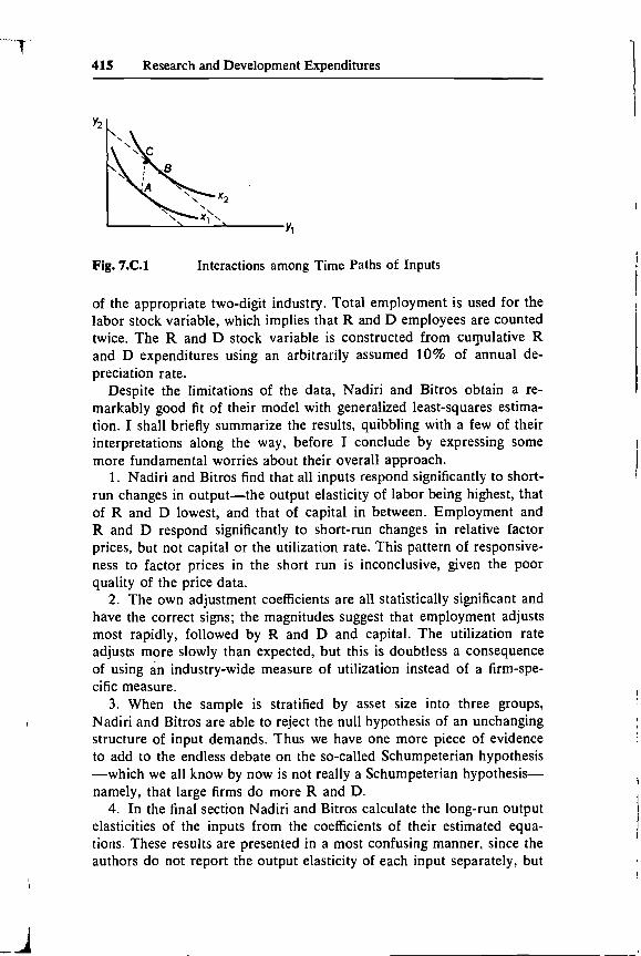
The first hypothesis seems appealing: that disequilibrium in factormarkets implies that firms fail to produce along their optimal expansionpaths. It seems quite reasonable to assume that output decisions areconstrained by input disequilibria. Nadiri and Bitros note that there isa third alternative which permits output to remain exogenous and firmsto be on the production function. This approach implies severe restric-tions on the adjustment coefficients. To illustrate, if output is exogenousa firm will move from output X1 to X2 in a certain time period (see fig.7.C. 1). If the production function constraint holds as an equality, thenthe firm must use a combination of inputs on the isoquant X2. If thedesired input combination is at point B, excess demand in the marketfor one factor will necessarily imply overshooting the target level of theother factor. In a model with several factors of production, at least onemust overshoot its target level to compensate for excess demand else-where.

This implied hypothesis of overshooting target values of one or moreinputs had considerably more intuitive appeal in the earlier work ofNadiri and Rosen than it does here. In Nadiri and Rosen (1973), utili-zation rates of each input entered directly (if perhaps too independently)into the production function. It seems quite reasonable to assume thatexcess demand for capital or labor would lead to an overshooting oftarget values of utilization rates, but it is not quite so obvious that stockswould overshoot in the same way. In the present paper, only the utiliza-tion rate of capital enters into the production function.

Nadiri and Bitros complete the model by substituting for the Y' termsin the adjustment equations an approximation to the factor demandfunctions derived from a Cobb-Douglas production function. Embeddedin the coefficients of the resulting system of equations are the estimatedvalues of the adjustment coefficients, and the elasticities of each inputwith respect to factor prices and output.

The model is estimated on pooled cross-section and time series dataon 62 firms for the period 1965—72. The limitations of the data are, asusual, serious. Wage rates at the two-digit industry level are used torepresent the user cost of both labor and R and D. The utilization rateis also an industry figure, rather than firm-specific. The output variablewas constructed by deflating firm revenues by the wholesale price index


Fig. 7.C.1 Interactions among Time Paths of Inputs

of the appropriate two-digit industry. Total employment is used for thelabor stock variable, which implies that R and D employees are countedtwice. The R and D stock variable is constructed from cumulative Rand D expenditures using an arbitrarily assumed 10% of annual de-preciation rate.

Despite the limitations of the data, Nadiri and Bitros obtain a re-markably good fit of their model with generalized least-squares estima-tion. I shall briefly summarize the results, quibbling with a few of theirinterpretations along the way, before I conclude by expressing somemore fundamental worries about their overall approach.

1. Nadiri and Bitros find that all inputs respond significantly to short-run changes in output—the output elasticity of labor being highest, thatof R and D lowest, and that of capital in between. Employment andR and D respond significantly to short-run changes in relative factorprices, but not capital or the utilization rate. This pattern of responsive-ness to factor prices in the short run is inconclusive, given the poorquality of the price data.

2. The own adjustment coefficients are all statistically significant andhave the correct signs; the magnitudes suggest that employment adjustsmost rapidly, followed by R and D and capital. The utilization rateadjusts more slowly than expected, but this is doubtless a consequenceof using an industry-wide measure of utilization instead of a firm-spe-cific measure.

3. When the sample is stratified by asset size into three groups,Nadiri and Bitros are able to reject the null hypothesis of an unchangingstructure of input demands. Thus we have one more piece of evidenceto add to the endless debate on the so-called Schumpeterian hypothesis—which we all know by now is not really a Schumpeterian hypothesis—namely, that large firms do more R and D.

4. In the final section Nadiri and Bitros calculate the long-run outputelasticities of the inputs from the coefficients of their estimated equa-tions. These results are presented in a most confusing manner, since theauthors do not report the output elasticity of each input separately, but

416 M. Ishaq Nadiri/ George C. Bifros

rather they report the sum of the elasticities of the inputs for each ofthe equations. These results suggest constant or increasing returns toscale. It would be useful to have separate calculations of the outputelasticity of each input.

5. Finally, the authors calculate what they interpret as the short,intermediate, and long-run responses of labor productivity by varyingin turn labor alone, then labor and R and D, and finally all factors.The meaning of this conceptual experiment is not entirely clear withinthe context of their model, which after all requires that all inputs mustvary in the short and intermediate runs. It would seem instead that ifthe authors were interested in the returns to R and D they would exam-ine the long-run elasticity of output with respect to R and D, which isa way of capturing how changes in R and D affect the productivity ofthe conventional inputs. This elasticity can be converted, with the appro-priate caveats mentioned by Professor Griliches in his paper, into a kindof crude average rate of return on R and D.

I would like to close with a more fundamental criticism of the paper.I have some difficulty in grasping the connection between the modelproposed by Nadiri and Bitros and the estimation techniques they em-ploy. In the version of the paper presented at the conference, the authorsheld to the pair of assumptions noted above: that firms are on the pro-duction function and that output is exogenous. They failed, however,to impose the appropriate restrictions on the the own and cross-adjustment coefficients. In an effort to remedy this deficiency, the au-thors have chosen to leave the adjustment coefficients unconstrainedand to treat output as endogenous. But merely asserting that output isendogenous and running two-stage least-squares does not get them outof the woods. Several problems remain:

1. If output is assumed to be endogenous, the behavioral assumptionof cost minimization given output is no longer appropriate. Presumably,this assumption would be replaced by profit maximization subject to theproduction function constraint, but this will introduce product price asan exogenous variable.

2. If output is endogenous and product price enters the model, it isnot obvious without further argument that the inferences made from theestimates about the parameters of the production function and the ad-justment equations will hold.

3. Since the estimated equations are neither the structural nor thereduced form, it is not clear that the error terms are appropriatelyspecified. If stochastic terms enter the structural equations in a simplelinear or multiplicative fashion, they will not enter linearly and inde-pendently in the equations estimated.

4. Even if the appropriate reduced-form equations were derived, theassumption that firms are on the production function suggests that the


error terms will not be independent across equations. Joint estimationimposing the appropriate restrictions would still be warranted.

While these problems are serious, they are in principle remediable.Despite these objections, this is a very interesting paper and an impor-tant further step toward building disequilibrium dynamics into the theoryof the firm. I hope the authors will further pursue this line of inquiry,with a richer data base if possible, using a more fully specified modeland appropriate joint estimation techniques.

Reference

Nadiri, M. Ishaq, and Rosen, Sherwin. 1973. A disequilibrium model ofdemand for factors of production. New York: National Bureau ofEconomic Research.

research and development expenditures and labor … · chapter title: research and development...

Documents