rescaling the life cycle: longevity and...

183

Rescaling the LifeCycle: Longevity andProportionality

RONALD LEE

JOSHUA R. GOLDSTEIN

Since 1900 life expectancy in the United States has increased by about 30years, from 48 to 77 years. Most projections foresee continued increase at aslower rate, reaching 85 or 90 years by 2100 (Lee and Carter 1992; Tuljapurkaret al. 2000). Some analysts foresee the possibility of far greater life expect-ancy increases—to 100, 150 years, or more (Manton et al. 1991; Ahlburgand Vaupel 1990; Schneider et al. 1990). Individuals welcome longer life,but for populations, increases of this magnitude could impose heavy costson the working-age groups and could have other substantial but uncertaineconomic and social consequences. These consequences will depend in largepart on how the additional expected years of life are distributed across thevarious social and economic stages of the life cycle. This chapter speculatesabout how the gains will be used and how the life cycle will be modified.

Proportional rescaling of the life cycle, in which every life cycle stageand boundary simply expands in proportion to increased life expectancy,provides a convenient benchmark. Under proportional rescaling, if longev-ity doubles, then so would childhood, the length of work and retirement,the span of childbearing, and all other stages of the life cycle. Proportionalrescaling of the life cycle would appear to be neutral in some sense, so thatlife, society, and economy could continue as before, except that there wouldbe proportionately more time spent in every stage. However, we will findthat while this is (or could be) true for some aspects of life, other aspectswould vary with the square or some other power of longevity.

Although proportional rescaling may seem natural, and indeed doesoccur in nature as we discuss, powerful forces impede its application to hu-mans. First are biological constraints related to human development, suchas menarche and menopause, even though our vigor and health may ad-vance with longevity. Second are institutional constraints, for example on

184 R E S C A L I N G T H E L I F E C Y C L E

schooling and retirement. Although these may adjust in the long run, overshorter horizons they may block proportional rescaling. Third, stock-flowinconsistencies may cause human and physical capital to rise with longev-ity more rapidly than labor force size, causing wages and incomes to riseand the interest rate and returns to human capital to fall, triggering furtheradjustments. If time in retirement is a luxury, then it may rise rapidly asincomes rise, so that age at retirement does not rise in proportion to lon-gevity—as in fact it has not. For these and other reasons, we should notactually expect to observe proportional rescaling in connection with in-creased life span in the past, nor should we anticipate it for the future. None-theless, proportionality is a useful benchmark against which to comparepast changes and the hypothetical future.

What would proportional rescaling look like?

A perfectly proportional rescaling of the life cycle accompanying increasedlife expectancy would appear indistinguishable from the effect of a simplechange in the units of measurement of age/time, as if we had changed fromdollars to pesos or from inches to centimeters. For example, suppose that anoriginal 75-year life cycle were instead measured in units of six lunar months,or half-years. The new life cycle would be 150 units long instead of 75, butof course nothing would be different. (We use doubling as a convenient ex-ample, but we believe that a 15 percent increase in life cycle is more likelyfor the twenty-first century.) Every life cycle stage would last twice as longas before, measured in the new units. Every rate would be only half as great,since only half as many events would take place in 6 months as in 12 months.

Proportional life cycle changes can occur in both strong and weak forms.In the strongest form, the change affects not only the average timing of lifecycle transitions but also the whole distribution of timing within a popula-tion. Thus, for example, the spread around the mean age of death or meanage of childbirth would also double if the mean age of death doubled. Wecall this “strong proportionality,” which can apply both to the distributionof an event among the individuals in a population and to the timing orlevel of an event in the individual life cycle. If the change in life cycle tim-ing is only proportional with respect to the mean ages of each life cycletransition or stage, then we call this “weak proportionality.” Weak propor-tionality would occur if, for example, as longevity increased, the mean ageof reproduction increased proportionately but the variance of the net ma-ternity function stayed constant.

It is important to distinguish between “flow” or “rate” variables, whichare measured per unit of time, and “stock” variables, which are not. Com-pleted fertility, accumulated wealth, the probability of ever marrying, or ofever having a first birth, are all examples of stocks. Birth rates, death rates,

R O N A L D L E E / J O S H U A R . G O L D S T E I N 185

wage rates, income, and rate of knowledge acquisition are flows, all mea-sured per unit of time. Under the perfectly proportional rescaling of the lifecycle discussed above, all stocks are unchanged, provided they are assessedat the same proportional stage of the life cycle (for example at the age equalto 60 percent of life expectancy). In a population with a life expectancytwice as great, the net reproduction rate (NRR) would not be twice as high;it would be unchanged. All flow or rate variables, however, would be re-duced in inverse proportion to the increase in longevity. Adding these re-duced rates across twice as long an age span of reproduction would thenyield an unchanged completed fertility.1 We might say that perfectly pro-portional rescaling of the life cycle is always “stock constrained,” in the sensethat the magnitude of stocks is preserved under rescaling.

In some cases, this kind of stock-constrained rescaling is not an inter-esting scenario to contemplate. For example, if people were to live twice aslong, we would not expect that at each age they would earn only half asmuch, or that they would learn only half as much during each year in school.In these cases, it is more natural to assume that the rate of productivity, orearning, or acquisition of knowledge, remains constant, so that the stock oflifetime earnings, or completed education, would double. Such cases wecall “flow constrained.”

Figure 1 illustrates some hypothetical examples of what proportionalrescaling would look like under different assumptions, all of which assumethe convenient, yet implausible doubling of longevity. The top row illus-trates strong proportionality with stock constraints, such as might be thecase with fertility. Here the ages at which flows occur are doubled, but atthe same time the flow itself is halved. The result is that lifetime completedfertility remains unchanged, although the age at which a given cumulativefertility is achieved is doubled. The middle row shows strong proportional-ity with flow constraints, such as might be the case with earnings. The ageat which a given flow occurs in the rescaled age profile is twice that of theoriginal profile. Keeping flows constant over a longer period of time, how-ever, produces a doubling of the stock, for example cumulative lifetime earn-ings (and perhaps derived stocks, such as lifetime savings, which we discusslater). The bottom row illustrates a particular case of weak proportionality.Here the mean age of the flow doubles from 25 to 50, but the width of theage profile does not expand proportionally.

Proportional rescaling in nature

The object of this chapter is to explore the feasibility of proportional rescalingwithin a single species, namely humans. A large body of work already existslooking at proportional rescaling between biological species. In biology thisfalls under the study of “biological invariants” (Charnov 1993). Figure 2 shows

FIGURE 1 Illustrative examples of proportional rescaling under ahypothetical doubling of longevity

Flows

0.00

0.02

0.04

0.06

0.08

0 20 40 60 80 100

Rat

e per

yea

rFlow-constrained strong proportionality

0.00

0.02

0.04

0.06

0.08

0 20 40 60 80 100

Rat

e per

yea

r

Age (years)

Weak proportionality

Stocks

0.0

0.5

1.0

1.5

2.0

0 20 40 60 80 100

Sto

ck a

t ag

e x

0.0

0.5

1.0

1.5

2.0

0 20 40 60 80 100

Sto

ck a

t ag

e x

Age (years)

NOTES: Original age profile is shown as a solid line, rescaled profile as dashed line. Stocks at age x arethe integral of flows from age zero to x. In this figure, flow-constrained strong proportionality isobtained by doubling ages at which a given rate is originally observed, resulting in a doubling ofeventual stocks; stock-constrained strong proportionality is obtained by simultaneously doubling agesand halving flows; and weak proportionality is obtained by doubling the mean of the flows whilekeeping the standard deviation of flows unchanged.

0.00

0.02

0.04

0.06

0.08

0 20 40 60 80 100

Rat

e per

yea

r

Stock-constrained strong proportionality

0.0

0.5

1.0

1.5

2.0

0 20 40 60 80 100

Sto

ck a

t ag

e x


an example of such an invariant across mammalian species: the relationshipbetween age at physical maturity (m) and expected years of adulthood e(m).Goldstein and Schlag (1999) show a similar figure for the relationship be-tween mean age of reproduction and life expectancy at birth. Other examplesof biological invariants include the ratio of body mass to life expectancy atbirth; the product of the number of offspring and the chance of survival tothe mean age of reproduction; and metabolic invariants (Austad 1997). “In-variant” is used by biologists not as a rule to which there are no exceptionsbut rather to describe general tendencies, with variation around them. Inmany cases, the rescaling involves a power transformation and is thereforenot proportional. For example, body mass rises approximately with the cubeof body length, so if body mass is proportional to life expectancy, then bodylength will not be. Note, however, that in equilibrium every animal popula-tion will have a net reproduction rate of unity, so this stock measure will beinvariant across species, consistent with proportional rescaling.

Biological invariants result from evolutionary forces, and explanationsfor them are given in terms of evolutionary theory and maximization ofreproductive fitness. The increased longevity of modern humans has notresulted from natural selection. It is the result of scientific advances, changesin life style, social organization, nutrition, and manmade environments. Forthis reason, we would not expect the biological invariants in nature to ap-

X

X

X

X

X

XX

X

X

X

X

X

X

X

X

X

X

XX

X

X

X

X

1.0

10.0

0.1

Expec

ted y

ears

of

adu

lth

ood e

(m)

Age at maturity (m)

beaver

vole

white-footed mouse

deer mouse

grey squirrelUinta ground squirrel

chipmunk

pica

rabbit

otterbobcat

skunk

zebra

impala

elk

wilde-beest

hippopotamus

waterbuck sheep

warthog

boar

buffalo

elephant

FIGURE 2 An example of proportional rescaling in nature: Age atmaturity versus expected life as a mature adult in 23 mammalianspecies (logarithmic scales)

NOTE: Data from Millar and Zammuto 1983.

0.2 0.5 1.0 2.0 10.05.0

0.5

2.0

5.0

20.0


ply to human life cycle timing as we live longer. Still, the analogy is useful,because the optimizing principle still obtains even if what is being optimizedis not reproductive fitness, but rather a more general notion of utility thatmight include economic as well as reproductive success and hedonic con-sumption as well as productive investments.

Furthermore, it appears that the evolution of proportionally relatedlife cycles across species is not a result of independent adaptations across arange of traits but is rather linked to some underlying biological mecha-nisms that control the rate of metabolism and other features of the life cycleclock (e.g., Carey et al. 1998; Finch 1990; Biddle et al. 1997; Lin et al. 1997).Evidence for this includes the ability to breed longer-living animals simplyby the selective breeding of individuals that reproduce late in life. The re-sult is that both the onset of reproduction and the age at death are propor-tionally delayed. Restricted diets in the laboratory appear to have a similareffect, delaying mortality but also delaying physical maturity. Finally, somegenetic modifications appear to have proportional effects on longevity andthe timing of reproduction.

Life table stretching and the proportional life cycle

We can divide the human life cycle into stages of childhood, working ages,and old age, marked approximately by the boundaries of age 15 or 20 and60 or 65. When life expectancy increases in a population, person-years oflife are added to the life table within each of these three life cycle stages,not only at the end of life in old age. This is not a natural way to thinkabout the lives of individuals; for individuals, alterations in length of lifeseem always to come at the end. But that is only so ex post; ex ante, indi-viduals are subject to risks of death at every age, and therefore their ex-pected years of life at each age throughout the potential life cycle are sub-ject to modification when these risks change.

Historically, we can observe at what ages person-years of survival areadded when life expectancy at birth has risen. When life expectancy has risenby one year from a low level such as 20, this one year has been distributed asfollows: 0.7 years between 15 and 65; 0.2 years between 0 and 15; and only0.1 year after 65. As life expectancy rises further, the incremental gains inchildhood and the working ages decline, and the gains in old age rise. Fur-ther increases from the current life expectancy level of 77 years in the UnitedStates will be concentrated in old age, with 0.7 years coming after age 65and hardly any coming before age 15 (Lee 1994; Lee and Tuljapurkar 1997).

Increasing survival does not affect all stages of life equally. A mechanicalreason for this is that in the above calculations we have not rescaled theage boundaries of youth and old age as longevity increased. But even if


these boundaries were rescaled, historical improvements of mortality havebeen inconsistent with proportional rescaling. Mortality has declined fasterin infancy than over the rest of the life cycle, and this has resulted innonproportional changes in the survival curve.

As with all other aspects of the life cycle, we can visualize strong pro-portional change by asking what would happen if we simply changed theunits of measuring age, say to 6-month units. Then for the proportion ofsurvivors, or for life expectancy, values would be attained at age x that werepreviously attained at age x/2. The higher the age in the initial life table,the farther out we would have to move on the new age scale to reach acorresponding level. For age x=3, the new age would be 6; and for age x=60,the new age would be 120. (Death rates would be shifted in the same way,but also proportionately reduced, as discussed earlier.)

To state this is to see that historical shifts have not corresponded to thissimple assumption. Fries (1980) emphasized that the actual pattern of mortal-ity change is of the opposite sort, and called it “compression of morbidity.”When mortality declines, the upper end of the l(x) curve shifts relatively little,rather than relatively more as required by strong proportionality. Indeed, someobservers suggest that the maximal length of life (first x such that l(x) = 0) hashardly changed at all in recent centuries. Wilmoth et al. (2000), however,show that the age of the oldest death in Sweden has been rising at least since1861, accelerating in recent decades; since 1970, it has been rising at aboutthe same speed as life expectancy (Wilmoth and Robine, in this volume.)

One useful diagnostic is to look at the l(x) value for some age x in1900, for example, and find the corresponding age at which that l(x) valueis reached in 1995.2 Calculation shows that comparing US mortality in 1900and 1995, the drop in survivorship reached at age 1 in 1900 was not matcheduntil age 59 in 1995, an age increase of 5,800 percent. The correspondingincreases at ages 30, 60, and 90 were 137 percent, 33 percent, and 10 per-cent. Under strong proportionality, these percent increases would be equalat all ages. We have made similar calculations for the projected survivor-ship changes between 1995 and 2080, based on the mortality projections ofthe Social Security Administration. The drop in survivorship reached at age1 in 1995 will not be matched until age 23 in 2080, an age increase of 2,200percent. The corresponding increases at ages 30, 60, and 90 are 50 percent,13 percent, and 5 percent.

We can get some analytic insight into the likely pattern of mortalitychange in the future by drawing on a simple result from Vaupel (1986).Suppose that mortality after age 50 follows Gompertz’s Law, with deathrates rising across age at a constant exponential rate q = 10 percent peryear. Suppose further that death rates at each age over 50 decline over timeat r = 1 percent per year. With these assumptions, mortality at ages over 50


declines in such a way that the mortality curve shifts r/q years to the rightevery year.3 With values of r = .01 and q = 0.1, the mortality curve shifts0.1 years to the right every year; and every decade, the death rate previ-ously experienced at age x will now be experienced at age x+1. Once mor-tality decline has proceeded to the point where survival to age 50 is close tounity,4 then the survival curve and life expectancy will be displaced to theright by one year each decade, at every year of age. Because this shift to theright is equal across all ages over 50, rather than increasing in proportion toage, it is not strictly consistent with proportional stretching.

Under proportional stretching of the life cycle, the time spent disabledor in ill health would rise in proportion to longevity, as would the time spentfree of disability. Recent research on disability, chronic illness, and functionalstatus reveals patterns that are broadly consistent with such proportionalchanges, at least for the last two decades in the United States (Costa 2000;Crimmins et al. 1997; Manton et al. 1997; Freedman and Martin 1999; Mantonand Gu 2001).5 For example, Crimmins et al. (1999) conclude that personsin their late 60s in 1993 are functionally like those in their early 60s in 1982.6

Research (Lubitz and Prihoba 1984; Lubitz et al. 1995; Miller 2001) also showsthat health care costs in old age are more closely related to time until deaththan to chronological age, so that as life expectancy rises and fewer personsat any age are near death, health care costs would fall, other things beingequal. All these findings are qualitatively consistent with proportional rescalingof the life cycle for health, functional status, and disability; but because ofimprecision of measure they are also consistent with compression of morbid-ity, with disabled years shrinking as a proportion of the life cycle.

Individual demographic aspects of rescaling

Mortality, survival, health, and longevity are the bare bones of the life cycle.Now we enrich the story by discussing fertility and other social behavior.

Transitions to adulthood: Education, marriage, and theonset of childbearing

In animals, the life cycle stage is often divided into infancy and maturityand is closely tied to physical growth and sexual maturity (Kaplan 1997).In humans, the transition to adulthood is typically seen as being much morecomplicated, involving a change in social, economic, and familial roles(Modell et al. 1976; Marini 1987). Sexual maturity is only the beginning ofthe transition to adulthood, which may be completed when children areeconomically and residentially independent of their parents, get married,and begin families of their own.


Some easily measured indicators of the transition to adulthood includethe age of educational completion, first marriage, and first birth. Table 1shows the pace of change of the mean ages of these indicators for severalindustrial countries between 1975 and 1995. Education, marriage, and child-bearing are all being postponed at a rapid pace in the United States, Japan,and Sweden.7 The rates of rescaling vary by indicator, but all are faster thanthe pace of longevity increase. Whereas life expectancy at birth is increas-ing roughly 0.2 percent per year, mean age at first birth is increasing abouttwice as fast, and mean age at first marriage perhaps four times as fast.

The differential rates of rescaling of education, marriage, and fertilitymean not only that the transition to adulthood as a whole is being shiftedto later ages but also that the interrelations between the various compo-nents of the transition are changing. For example, the faster pace of mar-riage postponement than of first births is evidence of the increase in pre-marital births and the rise of cohabitation in the United States and Sweden.The synchrony in marriage and birth postponement in Japan is due in partto low levels of premarital childbearing in that country.

The changing age profile of educational enrollment over the last half-century in the United States shows dramatic increases at both older andyounger ages. Figure 3 shows the percent enrolled in school by age groupamong the civilian noninstitutionalized population. We see massive increasesin enrollments in both the youngest age groups (3–4 and 5–6 years) andthe older age groups (above age 21). For older ages, the increases in enroll-ment correspond nicely to the proportional stretching scenario. The increasesin enrollment at younger ages, however, are not at all consistent with theproportional stretching argument, according to which the first ages of en-rollment should be increasingly postponed over time. One explanation ofincreased enrollment at younger ages is that it represents not so much a

TABLE 1 The pace of rescaling of selected life cycle indicators in theUnited States, Japan, and Sweden: Annual rates of change (in percent),1975 to 1995

Mean age at Mean age at Mean age at end ofLife expectancy first birth first marriage school enrollment

Country at birth (females) (women) (women) (both sexes)

United States 0.1 0.4 0.9 0.5Japan 0.4 0.3 0.3 0.3Sweden 0.2 0.5 0.7 NA

NOTES: (1) US ages at first birth and first marriage are period medians. (2) Mean age at end of school enrollment iscalculated from period enrollment rates. The mean age is estimated as m = sum(nEx * n) + x0, where nEx is theenrollment rate for the age group x to x+n (e.g., 31.9 percent for 20- and 21-year-olds in 1970), n is the width ofthe age group, and x0 is the youngest age group of full enrollment (age 6 in the US data). For Japan, entrance ratesto high school, junior college, and university were available. The mean age at end of school enrollment wasestimated as m = 14 + (4 * HS entry) + (2 * HS entry * Jr. college entry) + (4 * HS entry * university entry).SOURCES: Japan (1999, 2000); Sweden (1995); NCHS (2000).


change in the timing of the educational stage of the life cycle as an institu-tional shift from the private sphere of home education of infants to the publicsphere of day care and kindergarten. Still, if entry into a socializing envi-ronment (being surrounded by nonfamily members) is thought to be partof the transition from infancy to childhood, early enrollments represent anacceleration in life cycle timing.

While some of the transitions that signify the completion of entry intoadulthood, such as marriage and childbearing, are being delayed, many arebeing advanced to younger ages. Biologically, the long-term trend, untilrecently, has been earlier ages at menarche and physical maturity (Evelethand Tanner 1990). Legally, the trend worldwide is for voting rights to beextended to younger ages.8 Adult criminal penalties in both the United Statesand Japan are increasingly being extended to minors. Socially, precocious-ness appears to be the rule rather than the exception, with children allowedvarious forms of independence at increasingly younger ages.

Whereas half a century ago transitions to maturity were compressedinto a narrow age span, the transition appears to be becoming more diffuse.Children who move away from their parents increasingly return home(Goldscheider and Goldscheider 1999). Education, labor force participation,and the establishment of new families are often less clear-cut stages thanthey once were. People in their 20s and 30s may be working, going to school,

5 10 15 20 25 300

20

40

60

80

100

Per

cen

t en

rolled

Age

FIGURE 3 Educational enrollment rates in percent of civiliannoninstitutionalized population by age: United States 1947,1964, 1980, and 1998

1998

1947

1964

1980

SOURCE: US Census Bureau, Current Population Survey.(http://www.census.gov/population/socdemo/school/taba-2.txt)


receiving support from their parents, and starting a family of their own—allsimultaneously rather than in a series of ordered steps.

What are the implications of an expansion of early adulthood? Oneresult is a mismatch, at least temporarily, between certain life cycle–linkedinstitutions and the life cycle timing of individuals. As an example of this, inthe United States young adults can find themselves without health insur-ance because they are too old to be covered by their parents’ plans but arenot yet economically secure enough to have their own plans.

A second consequence of a longer transition to adulthood is more timefor career and partner searches. Social and sexual interactions with poten-tial spouses may now last a decade or more. Likewise, career experimenta-tion and repeated exit from and entry to education are possible thanks toless time pressure to support a family and achieve economic independence.Because the efficiency of searches probably remains constant per unit ofcalendar time (i.e., searches are flow constrained), the quality of searchesshould, all other things equal, improve.

A third consequence is the inversion of traditional sequences (Rindfusset al. 1987). A traditional sequence in the first half of the twentieth centurymight have been: educational completion, departure from parents’ home,entry into labor force, marriage, and childbearing. Now, with the extendedtime of the transition and the moving back and forth between transitions,childbearing may precede marriage; entry into the work force may precedeleaving the parental home; divorce may be followed by moving back to theparents’ home. The extended time over which the various transitions toadulthood occur allows greater opportunity to reverse transitions and tochange their order.

From the point of view of a rational life cycle planner, an extended pe-riod of quasi-adulthood probably makes sense for those who can expect tolive a long time. A long investment horizon makes it worthwhile to investmore in one’s own human capital and stay in school longer. Likewise, it makesexperimentation less costly and potentially more rewarding. It is not clearwhether time spent by 20- and 30-year-olds who have not yet committedthemselves to careers or to families is a productive human capital investmentor leisure (a kind of pre-career retirement). In some sense, it may be both.The prolonged period of transition to adulthood may be akin to the wrestlingof young chimpanzees, who look to us as if they are just playing but areactually learning skills that will be useful and necessary to them as adults.

Fertility

Over the course of the last century, increased longevity has been accompa-nied by declines in total fertility, without a consistent change in the meanage of childbearing.9 Delays in the timing of the first birth have been coun-


terbalanced by an earlier end of childbearing as the level of fertility hasdeclined. In recent decades, however, both the onset and end of childbear-ing have been slowly shifting to older ages. A continuation of this trend isconsistent with proportional stretching of the life cycle, but from a theo-retical perspective it is difficult to make firm predictions about either thetiming or the amount of fertility that will be associated with longer life.

As an example of the pattern of fertility change over the last century,Figure 4 shows age-specific fertility rates for women in the United States in1920, 1980, and 1998. The upper panels show the unadjusted age-specificfertility rates and the lower panels show the same age pattern, but normal-ized so that all of the curves have the same fertility level over the life cycle.The figure indicates that as fertility declined from 1920 to 1980, the timingof childbearing became more concentrated in the 20 to 25 year age group.

NOTE: Normalized profiles are obtained by dividing the age-specific rates in a given year by thetotal fertility rate in that year.

FIGURE 4 Period age-specific fertility profiles of US women:1920, 1980, and 1998

10 20 30 40 500.00

0.05

0.10

0.15

0.20

Fer

tility

rat

e

Age group

Fertility by age during decline

1920

1980

10 20 30 40 500.00

0.05

0.10

0.15

0.20

Fer

tility

rat

e

Age group

Fertility by age during postponement

1998

1980

10 20 30 40 500.00

0.02

0.04

0.06

0.08

Fer

tility

rat

e/TFR

Age group

Normalized fertility during decline

1920

1980

10 20 30 40 500.00

0.02

0.04

0.06

0.08

Fer

tility

rat

e/TFR

Age group

Normalized fertility during postponement

1998

1980


This was a result of declining fertility at both younger and older ages. Since1980, however, the whole distribution of fertility has shifted slightly to olderages. This recent shift is consistent with proportional change, in that birthrates at older ages are increasing faster than at younger ages.

Some believe that further increases in age at first birth will not be ac-companied by a proportional increase in the age at the end of childbearing.As a result the distribution of childbearing will be compressed to a narrowerband of the life cycle, increasingly between the ages of 30 and 40 years.One reason for believing such an assessment is the biology of female repro-duction and the onset of menopause, in which there has been little if anyrecorded change in the last century. A counterargument is that if biologicaladvances can extend life, then advances in reproductive technology can ex-tend childbearing. Already, the ability to store eggs and sperm, as well asfrozen embryos, suggests that parents can have children at arbitrarily lateages with the present technology. In the future, it may well be possible forwomen to conceive, gestate, and give birth to children at older ages. It doesnot seem a priori a more difficult problem to increase the age of women’smaximum reproduction than to increase the age of maximum longevity.

In the near term, proportional increases in the mean age of childbear-ing—weak proportionality—are possible even without advances in repro-ductive technology. For example, if female life expectancy were to increase25 percent to 100 years, the same proportional increase would require amean age of childbearing of 35, well within the realm of current biology.

Would later childbearing reduce total fertility? Timing may have a di-rect effect on the level of fertility, particularly if delays in the onset of fertilityare not accompanied, because of biological limits, by higher fertility at olderages. But later childbearing may also influence the demand for children.

Proportional rescaling could increase the costs of childbearing, boththe direct costs like children’s education and the indirect costs like the earn-ings and promotion opportunities forgone (Willis 1973; Calhoun andEspenshade 1988). Parents have higher potential earnings at older ages, solater births have a higher opportunity cost as participation in the labor forceis curtailed. Opportunity costs of childbearing will depend in part on howthe age-earnings curve is rescaled. But in some careers (e.g., academia andlaw firms) job security increases with age as a result of institutional prac-tices such as tenure. It may actually involve less sacrifice for some people tohave children at older ages, depending on institutional arrangements. Also,discounting will reduce the opportunity costs of later-born children.

Higher forgone earnings may be more than offset by higher lifetimeearnings, and the relative costs of childbearing may decrease. Furthermore,if the spacing of children does not change, there might be a substantial de-cline in the relative costs of bearing, say, two children. Consider a womanwho lives 75 years and has two children 3 years apart. She will be the mother


of children less than 3 years old for a total of 6 years out of her 75-year lifespan. On the other hand, a woman who lived to be 100 and had the samenumber of children with the same spacing would still only spend 6 years ofher life with infants. In this case the nonproportional change of the lengthof infancy resulting from the flow-constrained nature of human growth maychange the relative cost of childbearing.

Population-level implications of rescaling

The overlap of generations

Under perfect proportionality, population size and structure remain un-changed (Goldstein and Schlag 1999). However, if the mean age of repro-duction does not change at the same pace as longevity, then populationsize, the overlap of generations, and dependency ratios will be affected.

Consider a stylized life cycle in which childhood lasts until age 30,retirement begins at age 60, and everyone dies at age 90. Let reproductionoccur at age 30 and the population be stationary. In this case, three genera-tions will be alive at once, individuals will spend one-third of their life work-ing, and the total dependency ratio for the population as a whole will be2:1. Under proportional rescaling, say a doubling, none of these populationcharacteristics would change; population size would also remain constant.

If, on the other hand, longevity increased without changing genera-tional length, more generations would be alive at once and the total popu-lation size would increase. Such a nonproportional change would increasethe share of life spent between childbearing and retirement and would alsochange the total dependency ratio of the whole population. If we doubledthe length of life and the age of retirement as above but without changingthe age of reproduction, the number of generations alive at once wouldincrease from three to six, the population size would double, and the totaldependency ratio would shrink from 2:1 to 1:1. Nonproportional changesin generation length could also occur in the reverse direction. If generationlength increases faster than longevity, the result is a decline in populationsize and, if childbearing still signals the entry into adulthood, an increase inthe dependency ratio.

Is rescaling a solution for subreplacement fertility?

While the above discussion has assumed replacement-level fertility, it is per-haps of greater practical interest to consider how rescaling of the life cyclemight offset population aging that accompanies below-replacement fertil-ity. For example, age 65 in a stationary population might be mapped to age70 in a shrinking population, in order to keep retirees a constant propor-tion of the entire population.


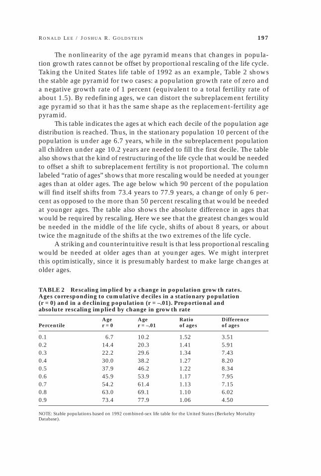
The nonlinearity of the age pyramid means that changes in popula-tion growth rates cannot be offset by proportional rescaling of the life cycle.Taking the United States life table of 1992 as an example, Table 2 showsthe stable age pyramid for two cases: a population growth rate of zero anda negative growth rate of 1 percent (equivalent to a total fertility rate ofabout 1.5). By redefining ages, we can distort the subreplacement fertilityage pyramid so that it has the same shape as the replacement-fertility agepyramid.

This table indicates the ages at which each decile of the population agedistribution is reached. Thus, in the stationary population 10 percent of thepopulation is under age 6.7 years, while in the subreplacement populationall children under age 10.2 years are needed to fill the first decile. The tablealso shows that the kind of restructuring of the life cycle that would be neededto offset a shift to subreplacement fertility is not proportional. The columnlabeled “ratio of ages” shows that more rescaling would be needed at youngerages than at older ages. The age below which 90 percent of the populationwill find itself shifts from 73.4 years to 77.9 years, a change of only 6 per-cent as opposed to the more than 50 percent rescaling that would be neededat younger ages. The table also shows the absolute difference in ages thatwould be required by rescaling. Here we see that the greatest changes wouldbe needed in the middle of the life cycle, shifts of about 8 years, or abouttwice the magnitude of the shifts at the two extremes of the life cycle.

A striking and counterintuitive result is that less proportional rescalingwould be needed at older ages than at younger ages. We might interpretthis optimistically, since it is presumably hardest to make large changes atolder ages.

TABLE 2 Rescaling implied by a change in population growth rates.Ages corresponding to cumulative deciles in a stationary population(r = 0) and in a declining population (r = –.01). Proportional andabsolute rescaling implied by change in growth rate

Age Age Ratio DifferencePercentile r = 0 r = –.01 of ages of ages

0.1 6.7 10.2 1.52 3.510.2 14.4 20.3 1.41 5.910.3 22.2 29.6 1.34 7.430.4 30.0 38.2 1.27 8.200.5 37.9 46.2 1.22 8.340.6 45.9 53.9 1.17 7.950.7 54.2 61.4 1.13 7.150.8 63.0 69.1 1.10 6.020.9 73.4 77.9 1.06 4.50

NOTE: Stable populations based on 1992 combined-sex life table for the United States (Berkeley MortalityDatabase).


Rescaling and economic behavior:Retirement trends

As life expectancy rises and health at older ages improves, it seems naturalthat the age at retirement should rise as well. For example, in assessing theeffects of longer life, Kotlikoff (1981) makes two alternative assumptions:that the age at retirement rises in proportion to life expectancy at birth, oralternatively that it rises more than in proportion to life expectancy at birth,to keep the years of retirement at the end of life constant. In fact, however,in industrial countries age at retirement and older men’s labor force partici-pation rates have been dropping for more than a century, while life expect-ancy has risen by several decades (Costa 1998). In the United States in 1900,men retired in their early 70s, on average, compared with age 63 today(National Academy on an Aging Society 2000: 6). Labor supply at olderages has also declined sharply in developing countries (Durand 1977).

According to the US period life table for 1900, the ratio of the ex-pected years lived after age 70 to those lived during ages 20 through 69 is0.10. For each year spent working, 0.1 years would have been spent re-tired.10 If retirement in 1995 still occurred at 70, mortality decline since1900 would have raised this ratio from 0.10 to 0.23. Given that the meanretirement age actually has fallen to 63 for men, the ratio in 1995 of ex-pected retirement years to expected work years has risen from 0.10 to 0.38,nearly quadrupling since 1900. In order to maintain the original ratio of0.10 over the life cycle, the retirement age in 1995 would have to be movedto 78. If we were to allow for an earlier age at start of work in 1900, theresults would be even more dramatic. While retirement age has stoppedfalling in the United States during the past decade, and has even modestlyrisen, the long-term trend has been strongly downward.

Ausubel and Grubler (1995) examined long-term trends, 1870 to 1987,in average hours worked over the life cycle for France, Germany, GreatBritain, the United States, and Japan. They calculated disposable lifetimehours as 24 *365e

10, less 10 * 365e

10 for physiological time (sleeping, eating,

hygiene). For sexes combined in Great Britain from 1857 to 1981, they foundthat lifetime work hours declined from 124,000 to 69,000, while disposablenonwork hours increased from 118,000 to 287,000. Work as a share of to-tal disposable hours (that is, work as a share of total lifetime nonphysiologicalhours above the age of 10) declined from 50 percent to 20 percent.11

Of course, much has happened over this period besides the increase inlongevity. Growth in financial institutions and in public and private pen-sions has made it easier to provide for consumption in retirement. Incomehas increased and educational attainment has risen. Given these changes, itis perhaps not surprising that retirement age has fallen. Leisure is presum-ably a luxury good. We would expect its share of the life cycle budget to


grow as income rises secularly. If life expectancy and health status had in-creased while hourly wages remained constant, then a decline in retire-ment age would seem unexpected. In this counterfactual case, we wouldprobably expect a proportional increase in both work time and leisure time,to keep their marginal contributions to lifetime utility equal.

There is also abundant evidence that institutions and employers’ prac-tices have encouraged earlier departure from the labor force than individu-als might have chosen otherwise. Discrimination against older workers usedto be common. In the United States it has been addressed by a series oflegislative acts of states going back to the 1930s and since the 1960s byfederal law (Neumark 2001). The incentives for early retirement in em-ployer-provided defined-benefit pensions are also important (see e.g.,Lumsdaine and Wise 1994; Wise 1997). Strong incentives are also built intomany defined-benefit public pensions, particularly when these are combinedwith incentives arising from tax policies, long-term unemployment ben-efits, and disability benefits. In a striking cross-national study of 11 OECDcountries, Gruber and Wise (1997) found that in some countries the com-bined effect of such policies makes the net wage for continuing work afterage 60 years drop close to zero or even turn negative, a very heavy “im-plicit tax.” They found that this implicit tax accounts for most of the varia-tion across countries in labor force participation rates at older ages.12

In sum, a combination of economic and institutional change, distortedincentives, and the behavioral response to these has caused the proportionof the life cycle devoted to work to shrink dramatically.

Rescaling and the economy

Consider now the effect of proportional rescaling on the economy, taking adoubling of life expectancy as a convenient, albeit implausible example.Under stock-constrained proportional rescaling, all flow variables would beonly half as great, including wages, gross domestic product, and consump-tion and savings per unit time. Stock variables like capital would be unaf-fected at corresponding ages over the life cycle (that is, at ages representingthe same proportion of life expectancy). The tax rate that would be requiredfor the working-age population to support the retirement of the elderlythrough pay-as-you-go public pensions would remain the same at corre-sponding ages.

On reflection, however, this stock-constrained expansion of the life cycleis neither realistic nor appealing. When we hypothetically changed the mea-sure of time from years to six-month units, in fact nothing changed, althoughall flow measures were halved. But if life expectancy were in fact to double,our unit of measure would nonetheless remain the year. In this case, wewould not expect that output per year would be halved; nor wage rates, an-


nual consumption, or savings. If people were to work twice as many yearsconsistent with the proportionality assumption, then their lifetime earningswould be roughly twice as great (more or less, depending on returns to expe-rience versus obsolescence of skills and knowledge), as would their lifetimeconsumption and savings. The cumulation of savings over twice as many yearswould generate assets at retirement that would be twice as large—as theyshould be, in order to finance a retirement that would be twice as long.

Figure 5 illustrates the implications for capital accumulation and thecapital/labor ratio. The age at beginning work is denoted A; it will vary whenlongevity varies, but is treated as fixed for purposes of this figure. In a sta-tionary population with one person born into each generation, the size ofthe labor force will initially be the distance AB. Accumulated wealth, heldas capital, will grow linearly over the life cycle to amount F, and then bespent-down to fund retirement until death at age C, when it is exhausted.13

The total stock of capital in the economy will be the area of the triangleAFC. The capital/labor ratio is this area divided by the number of workers,AB. Now suppose life expectancy doubles from AC to AE, and the age atretirement doubles from B to D. The new labor force is AD (continuing to

FIGURE 5 The nonproportional consequences of proportional rescaling on the aggregate economy: Earnings, savings, and the capital/labor ratio

NOTE: In the short life cycle, people begin work at age A and retire at age B having accumulated amount F to support their retirement until death at C. The capital/labor ratio is the area of triangle AFC divided by the number of laborers AB in a stationary population. In the doubled life cycle, people retire at D having accumulated amount G to support them in their longer retirement until death at E. The capital/labor ratio is the area of the triangle AGE divided by the number of workers in the stationary population, AD. If the generation size remains constant, there are twice as many workers with the doubled life cycle, since length AD is twice AB. However, there is four times as much capital, since G is twice F, and E is twice C. Therefore, the capital/labor ratio is twice as great. This assumes life cycle savings behavior, with constant earnings by age and zero interest.

A B C D E

Age

Acc

um

ula

ted w

ealt

h

F

G


assume one person per generation), and the new capital stock is the area ofthe triangle AGE. Since both the base and the height of AGE are twice asgreat as the corresponding dimensions of AFC, its area is four times as great.However, the labor force is only twice as great, so the new capital/laborratio is twice the old.

The productivity of labor will be higher because of the increased capitalper worker, so wages and gross domestic product will also rise, but by lessthan a factor of two owing to diminishing returns. The higher wages willfurther raise the capital per worker. The total effect might be to raise percapita income and wage rates by about 40 percent.15 More capital per workerwill mean a lower marginal productivity of capital, and lower profit rates andinterest rates. Lower interest rates will in principle alter decisions about howto allocate consumption over the life cycle and savings decisions.

It also is not plausible to expect the acquisition of knowledge by anenrolled student to occur at only half the rate after a rescaling of the lifecycle as it did before, as strict proportional rescaling would require. If thetime in school doubles, we would also expect the stock of knowledge ac-quired to roughly double. Longer education and greater knowledge wouldalso raise the productivity of labor and wages throughout the life cycle, in-teracting with the effects of capital that were just discussed. What wouldthen happen to the rate of return to education, which provides the incen-tive for people to invest in learning? Longer life would increase the paybackperiod, tending to raise the rate of return. However, returns would be de-creased by the greater quantity of education. It is also unclear how the lifecycle trajectory of labor earnings would be affected, given that accumula-tion of experience contends with obsolescence of knowledge and skills.

In sum, the proportional expansion of the life cycle does not makesense once we take into account some basic economic ideas. Life cycle ex-pansion, even with proportionality, would imply increased human andphysical capital per worker, lower profit rates and interest rates, higher wagesand per capita incomes, and altered returns to education and altered lifecycle earning trajectories.

How might rising per capita incomes affect people’s choices? Ofteneconomists assume that the preference functions governing choices amonggoods and activities are homothetic, meaning that as incomes rise, the util-ity tradeoffs (marginal rates of substitution) between items do not change ifgoods are consumed in the same proportion. Such an assumption here wouldpreserve a proportional expansion of some aspects of the life cycle, despiterising incomes. When we think about saving behavior—trading off consump-tion today against consumption in old age, for example—this assumptionmay be defensible. However, it is more questionable in the context of thetradeoff between consumption and leisure, which will influence hoursworked per day as well as the decision about when to retire.


Conclusions

We have explored the consequences of longer life for the timing of life cycleevents between birth and death. We have used proportional rescaling as abaseline against which to compare the actual past and the potential future.Proportionality is not inevitable. In many cases, it is not even likely. In al-most no case is the timing of life cycle events changing at exactly the samepace as longevity itself is increasing. Still, proportional rescaling provides astarting point, a simple framework, from which to view the largely unex-plored consequences of increasing longevity for the timing of different seg-ments of life. We do not suggest that all the changes we considered aredirectly or indirectly caused by increased longevity. In some cases there areplausible links, but in many cases the causes of change are not in any obvi-ous way connected to mortality change.

In order to get the broadest picture, it is useful to set aside issues ofthe exact pace at which changes are occurring and to ask simply which lifecycle stages are changing in a direction consistent with proportionality. Aswe live longer, we are indeed spending more time in school, staying singlelonger, delaying reproduction, delaying entry into the work force, and stayinghealthy longer. On the other hand, childhood at least as it is socially de-fined is not lengthening, and working life has shrunk. Biologically, humangrowth, maturity, and menopause have remained nearly fixed, even as lifehas been extended.

The barriers to proportional rescaling are behavioral, institutional, andbiological. From a behavioral point of view, people have chosen to allocateincreasing shares of life to leisure. As we have seen over the last century,longer and wealthier life has been accompanied by proportionately moreyears spent in leisure, not fewer. Although population aging may not allowthe historic trend toward earlier retirement to continue, it is likely that lei-sure time, perhaps spent not only in retirement but also before entry intothe labor force and perhaps during the working years, will increase at afaster than proportional rate with increased longevity.

Institutions also form barriers to proportional rescaling. For example,incentives for early retirement have grown with the generosity of pensionprograms in recent decades, amplifying the behavioral effects. Similarly, age-graded eligibility, whether it be for insurance, military service, or tax treat-ment, makes the timing of life cycle stages less elastic than it might other-wise be. Institutions may ultimately adapt to behavioral preferences, butthey will do so slowly.

Finally, biological barriers to proportional rescaling appear. Becauseincreased longevity is not a result of evolutionary forces that fundamen-tally change human biology, changes in mortality rates are not accompa-nied by changes in the timing of human growth, the length of time infants


are physically dependent on their parents, sexual maturity, or menopause.Human aging may be slowing, but this is not yet influencing the timing ofhuman development. However, biological constraints do not yet block pro-portional increases, at least in terms of weak proportionality, in the timingof reproduction. The mean age of childbearing could rise considerably be-fore it reached current biological limits.

This chapter only touched on the wide range of issues that increasinglongevity might imply for the reorganization of human life. Among the manyworthwhile topics to pursue are the consequences of rescaling for a num-ber of life cycle models. Mincer’s (1974) formulation of human capital ac-cumulation might be explored, looking specifically at the effect of propor-tional increases in education on entry into the labor force and on the ageprofiles of earnings. Under what conditions would the earnings peak itselfmove proportionally? What would happen to lifetime income? What wouldbe the consequences for the opportunity costs of childbearing? A secondarea for research is the aggregate economic consequences of longer life. Wehave seen that even under proportionality, the consequences of longer lifeare not economically neutral, since human and physical capital per personwould grow with the square of longevity. Further investigation of the equi-libria implied by both proportional rescaling and different scenarios of non-proportional change would be revealing.

Another issue to consider is the plausibility of repetition as an alterna-tive to elongation of life cycle states. To some extent, the increase in remar-riage and in formation of “second” families suggests that many aspects oflife may not be so constrained as we have suggested from our emphasis onstock constraints. Several distinct periods of schooling could be an alterna-tive to simply adding years of schooling at the beginning of life. One couldimagine that several careers, several families, and several hometowns couldemerge with increased longevity. The viability of the repetitive life cycle asopposed to the elongated life cycle will depend on economic factors such asthe depreciation rate of human capital with time, the earnings trajectoryand value of experience in a particular career, and changing perceptions ofsocial issues that make the unity of the life course a defining element ofhuman identity. Perhaps the repeated life cycle may be psychologically un-appealing, if the value of social networks of family, neighbors, and colleaguesis so strong as to make full replacement impossible.

Finally, rescaling confronts measures of time that are external to thehuman life cycle. For many animals and plants, the length of the seasons isa fundamental unit of time, an underlying metronome that does not allowcontinuous rescaling. For humans, underlying pacemakers of life, externalto human behavior, are some of the main obstacles to simple proportionalchange. Human skills degrade at some rate with nonuse, we learn at somerate, children grow up at some rate, social bonds are created and dissolved


at some rate, technology changes at some rate, and so forth. To a large ex-tent, the effect of longer life on the rescaling and reorganization of the lifecycle will be determined by what happens to people’s valuation of time in ageneral sense. The economic value of time in terms of productivity and earn-ings is one aspect of this. Another aspect is the various units of time: theworkweek, the school year, and other rhythms of human life.

Notes

The first author’s research for this chapter wasfunded by a grant from NIA, R37-AG11761.

1 As an example, consider the life tablesurvival function, l(x), and the density of deathsat age x, d(x). Consider a proportional rescalingsuch that new age y equals x/c. If the new func-tions are l* and d*, then for c=2 we would havel*(100) = l(50). That is, under the new mortal-ity regime, the proportion of people now sur-vive to 100 that used to survive to 50. The den-sity of deaths is given by d(x) = –dl(x)/dx(where the d for derivative should not be con-fused with the d for deaths). It follows thatd*(x) = (1/c)d(x/c). That is, not only is the d(x)curve stretched out, but its level is also reducedby the factor 1/c at each x. d(x) is stock con-strained, because it must integrate across all agesto 1.0 or to the radix of the life table.

2 Another way to assess proportionalstretching is to plot the old and new survivalcurves against the logarithm of age. The samehorizontal displacement will then correspondto a proportionate increase in age from anystarting point. Under strong proportionality,the horizontal distance between the two sur-vival curves should be a constant, in our ex-ample equal to log(2). If the two curves beingcompared are rates, expressed per unit time,then the new curve should first be multipliedby c before plotting against the logarithm ofage (see note 1 above).

3 Formally, for any s, m(x,t) = m(x+rs/q,t+s).

4 The probability of surviving to age 50in the 1995 period US life table for sexes com-bined was .925, and it is projected to be .965in 2080.

5 Costa (2000) reports that from the earlytwentieth century to the 1990s, the average rateof functional disability for men aged 50 to 74

declined at 0.6 percent per year. Crimmins etal. (1997) have found similar rates of declinefor recent decades, while Manton et al. (1997)and Freedman and Martin (1999) find consid-erably more rapid rates of decline, and Mantonand Gu (2001) report accelerating rates of de-cline in chronic disability since 1982.

6 Analyses of data from the Social Secu-rity disability insurance program (DI) tell a dif-ferent story, but those disability rates are domi-nated by behavioral responses to the incentivesof the program and appear to be less relevantthan direct measures of illness or functionalstatus.

7 Couple formation, particularly in Swe-den, is poorly measured by marriage alone,since cohabitation is so common. Levels of co-habitation are lower in the United States, andlower still in Japan.

8 For example, both Sweden and theUnited States lowered their voting ages from21 to 18 during the 1960s and 1970s.

9 The baby boom years following WorldWar II were accompanied by a dip in the meanage of childbearing.

10 Note that it is incorrect to base a calcu-lation of this sort on the change in life expect-ancy at age 65. The probability of survivingfrom age 20 to age 65 increased from 0.52 in1900 to 0.82 in 1995, for example. The cor-rect calculation is based on T65/(T20–T65),which is the ratio of years lived after age 65 tothose lived during ages 20–64 over the indi-vidual life cycle. These calculations do not takeinto account the distribution around the meanage of retirement.

11 Unfortunately, Ausubel and Grublerworked with life expectancy and not survivaldistributions, an approach that exaggerates thesize of these proportional declines in work time.


References

Ahlburg, Dennis and James Vaupel. 1990. “Alternative projections of the U.S. population,”Demography 27(4): 639–652 (November).

Austad, Steven N. 1997. Why We Age: What Science Is Discovering about the Body’s Journey ThroughLife. New York: J. Wiley & Sons.

Ausubel, Jesse and Anrulf Grubler. 1995. “Working less and living longer: Long-term trendsin working time and time budgets,” Technological Forecasting and Social Change 50(3):195–213.

Bongaarts, John and Griffith Feeney. 1998. “On the quantum and tempo of fertility,” Popu-lation and Development Review 24(2): 271–291.

Biddle, F. G., S. A. Eden, J. S. Rossler, and B. A. Eales. 1997. “Sex and death in the mouse:Genetically delayed reproduction and senescence,” Genome 40: 229–235.

Carey, J. R. et al. 1998. “Dual modes of aging in Mediterranean fruit fly females,” Science281: 996–998.

Calhoun, Charles A. and Thomas J. Espenshade. 1988. “Childbearing and wives’ foregoneearnings,” Population Studies 42(1): 5–37.

Charnov, Eric L. 1993. Life History Invariants: Some Explorations of Symmetry in EvolutionaryEcology. New York: Oxford University Press.

Costa, Dora. 1998. The Evolution of Retirement: An American Economic History, 1880–1990. Chi-cago: University of Chicago Press.

———. 2000. “Long-term declines in disability among older men: Medical care, public health,and occupational change,” National Bureau of Economic Research, Working PaperSeries W7605 (NBER, Cambridge, MA), pp. 1–40.

Crimmins, Eileen, Yasuhiko Saito, and Dominique Ingegneri. 1997. “Trends in disability-free life expectancy in the United States, 1970–90,” Population and Development Review23(3): 555–572.

Crimmins, Eileen, Sandra L. Reynolds, and Yasuhiko Saito. 1999. “Trends in the healthand ability to work among the older working-age population,” Journal of Gerontology54B(1): S31–S40.

Durand, John. 1977. The Labor Force in Economic Development. Princeton, NJ: Princeton Uni-versity Press.

Eveleth, Phyllis B. and J. M. Tanner. 1990. Worldwide Variation in Human Growth. Cam-bridge: Cambridge University Press.

12 The public pension programs in theUnited States and Japan stand out has havingrelatively little incentive for early retirement.In the US, at least, many employer-providedplans do have strong incentives, however.

13 Consumption in old age may also befunded in part by transfers from workers, aswith pay-as-you-go public pension systems. Theargument in this paragraph applies to the por-tion of consumption in retirement that is fundedthrough private savings or employer-providedpensions. For simplicity the calculations ignorethe return to investments in capital.

14 Under stock-constrained proportionalstretching, the flow of births would actuallybe only half as great as before, so there would

be only one-half person per generation. Thetotal labor force size would be unchanged, butthere would be twice as much capital, since theaverage worker holds twice as much capital ascan be seen from Figure 5. All that really mat-ters is the ratio of capital to labor, so the size ofgenerations in the stationary population is ir-relevant.

15 Suppose that per capita income is pro-portional to the capital/labor ratio raised to the1/3 power, a standard assumption, and that thenew capital/labor ratio equals the old times 2times the ratio of new to old per capita income.Solving, we find that the ratio of per capita in-comes equals the square root of 2, or about a40 percent increase.


Finch, C. E. 1990. Longevity, Senescence, and the Genome. Chicago: University of Chicago Press.Freedman, Vicki and Linda Martin. 1999. “The role of education in explaining and fore-

casting trends in functional limitations among older Americans,” Demography 36(4):461–473 (November).

Fries, James. 1980. “Aging, natural death, and the compression of morbidity,” The New En-gland Journal of Medicine 303: 130–136.

Funatsuki, Kakuchi. 2000. “Big changes seen under new juvenile law,” Yomiuri Shimbun, 2Nov., p. 3.

Goldscheider, Frances and Calvin Goldscheider. 1999. The Changing Transition to Adulthood:Leaving and Returning Home. Thousand Oaks, CA: Sage Publications.

Goldstein, Joshua R. and Wilhelm Schlag. 1999. “Longer life and population growth,” Popu-lation and Development Review 25(4): 741–747.

Gruber, Jonathan and David Wise. 1997. “Introduction and summary,” Social Security Pro-grams and Retirement Around the World. Cambridge, MA: National Bureau of EconomicResearch, Working Paper Series, W6134.

Japan National Institute of Population and Social Security Research (Kokuritsu Shakai HoshoJinko Mondai Kenkyujo). 2000. Latest Demographic Statistics (Jinko tokei shiryoshu),Research Series No. 299, 20 September.

Japan Ministry of Health, Labor and Welfare (Koseisho Daijin Kambo Tokei Chosabu). 1999.Vital Statististics of Japan 1999, Volume 1 (Jinko dotai tokei).

Kaplan, Hillard. 1997. “The evolution of the human life course,” in Kenneth W. Wachterand Caleb E. Finch (eds.), Between Zeus and the Salmon: The Biodemography of LongevityWashington, DC: National Academy Press, pp. 175– 211.

Kaplan, Hillard and D. Lam. 1999. “Life history strategies: The tradeoff between longevityand reproduction,” paper presented at the Annual Meeting of the Population Associa-tion of America, New York, March.

Kotlikoff, Laurence. 1981. “Some economic implications of life span extension” in J. Marchand J. McGaugh (eds.), Aging: Biology and Behavior. New York: Academic Press, pp.97–114. Reprinted as Chapter 14 in What Determines Savings? Cambridge, MA: MITPress, pp. 358–375.

Lee, Ronald. 1994. “The formal demography of population aging, transfers, and the eco-nomic life cycle,” in Linda Martin and Samuel Preston (eds.), The Demography of Aging.Washington, DC: National Academy Press, pp. 8–49.

Lee, Ronald and Lawrence Carter. 1992. “Modeling and forecasting U.S. mortality,” Journalof the American Statistical Association 87(419): 659–671.

Lee, Ronald and Shripad Tuljapurkar. 1997. “Death and taxes: Longer life, consumption,and social security,” Demography 34(1): 67–82.

Lin, K., J. B. Dorman, A. Rodan, and C. Kenyon. 1997. “Daf-16: An HNF-3/forkhead fam-ily member that can function to double the life span of Caenorhabditis elegans,” Science278: 1,319–1,332.

Lubitz, J. and R. Prihoba. 1984. “The use of Medicare services in the last two years of life,”Health Care Financing Review 5: 117–131.

Lubitz, J., J. Beebe, and C. Baker. 1995. “Longevity and medicare expenses,” New EnglandJournal of Medicine 332: 999–1,003.

Lumsdaine, Robin L. and David A. Wise. 1994. “Aging and labor force participation: A re-view of trends and explanations,” in Yukio Noguchi and David Wise (eds.), Aging inthe United States and Japan. Chicago: University of Chicago Press, pp. 7–41.

Manton, Kenneth, Eric Stallard, and H. Dennis Tolley. 1991. “Limits to human life expect-ancy: Evidence, prospects, and implications,” Population and Development Review 17(4):603–638.

Manton, Kenneth, Larry Corder, and Eric Stallard 1997. “Chronic disability trends in eld-erly United States populations: 1982–1994,” Proceedings of the National Academy of Sci-ences 94: 2,593–2,598.


Manton, Kenneth and XiLiang Gu. 2001. “Changes in the prevalence of chronic disabilityin the United States black and nonblack population above age 65 from 1982 to 1999,”Proceedings of the National Academy of Sciences 98(11): 6,354–6,359.

Marini, M. M. 1987. “Measuring the process of role change during the transition to adult-hood,” Social Science Research 16: 1–38.

Millar, J. S. and R. M. Zammuto. 1983. “Life histories of mammals: An analysis of life tables,”Ecology 64: 631–635.

Miller, Tim. 2001. “Increasing longevity and Medicare expenditures,” Demography 38(2):215–226.

Mincer, Jacob. 1974. Schooling, Experience, and Earnings. New York: Columbia University Press,for the National Bureau of Economic Research.

Modell, John, Frank F. Furstenberg, Jr., and Theodore Hershberg. 1976. “Social change andtransitions to adulthood in historical perspective,” Journal of Family History 1: 7–32.

National Center for Health Statistics. 2000. Vital Statistics of the United States, 1997, Volume I,Natality, Third Release of Files «http://www.cdc.gov/nchs/datawh/statab/unpubd/natal-ity/natab97.htm» Table 1–5. Median age of mother by live-birth order, according torace and Hispanic origin: United States, selected years, 1940–97 (released 8/2000).

National Academy on an Aging Society. 2000. “Who are young retirees and older work-ers?” Data Profiles: Young Retirees and Older Workers, June, no. 1.

Neumark, David. 2001. “Age discrimination legislation in the United States,” National Bu-reau of Economic Research, Working Paper Series 8152 (NBER, Cambridge, MA), pp.1–44.

Rindfuss, Ronald R., C. Gray Swicegood, and Rachel A. Rosenfeld. 1987. “Disorder in thelife course: How common and does it matter?” American Sociological Review 52(6): 785–801.

Schneider, Edward L. and Jack M. Guralnik. 1990. “The aging of America: Impact on healthcare costs,” Journal of the American Medical Association 263(17): 2,335–2,340.

Shoven, John B., Michael D. Topper, and David A. Wise. 1994. “The impact of the demo-graphic transition on government spending,” in David Wise (ed.), Studies in the Eco-nomics of Aging. Chicago: University of Chicago Press, pp. 13–33.

Sweden. Central Statistical Bureau. 1995. Population Statistics 1995 (Befolkningsstatistik 1995),Volume 4.

Tuljapurkar, Shripad, Nan Li, and Carl Boe. 2000. “A universal pattern of mortality declinein the G-7 countries,” Nature 405: 789–792.

Vaupel, J. W. 1986. “How change in age-specific mortality affects life expectancy,” Popula-tion Studies 40(1): 147–157 .

Willis, Robert J. 1973. “A new approach to the economic theory of fertility behavior,” Jour-nal of Political Economy 81(2): S14–S64.

Wilmoth, John R., Leo J. Deegan, Hans Lundström, and Shiro Horiuchi. 2000. “Increase ofmaximum life-span in Sweden, 1861–1999,” Science 289: 2,366–2,368.

Wise, David. 1997. “Retirement against the demographic trend: More older people livinglonger, working less, and saving less,” Demography 34(1): 83–96.

rescaling the life cycle: longevity and...

Documents