requirements for the validation of analytical methods b gtfch... · 3 1 introduction the validation...

APPENDIX B

To the GTFCh Guidelines for quality assurance in

forensic-toxicological analyses

Requirements for the validation of analytical methods

Authors: F. T. Peters, Jena; M. Hartung, Homburg/Saar; M. Herbold u. G. Schmitt,

Heidelberg; T. Daldrup, Düsseldorf; F. Mußhoff, Bonn

Revised by: F. T. Peters, Jena und L. D. Paul, München, in cooperation with the other

members of the subgroup „Guidelines of the working group Quality Control”: F.

Mußhoff, Bonn; B. Aebi, Bern; V. Auwärter, Freiburg; T. Kraemer, Homburg; G.

Skopp, Heidelberg.

Version 01

Date: 1st of June 2009

Table of contents

1. Introduction .......................................................................................................3

2. Court-proof, identifying and confirmatory procedures ...............................................4

2.1 Selectivity ..................................................................................................4

2.2 Linearity of Calibration, after Ref. [8] ...........................................................5

2.2.1 Calibration range, after Ref. [12] ..........................................................5

2.3 Accuracy, after Ref. [12] ............................................................................6

2.3.1 Systematic error (bias) and Trueness, after Ref. [12] ...............................7

2.3.2 Precision, after Ref. [12] ....................................................................7

2.3.2.1 Repeatability, after Ref. [10]................................................................7

2.3.2.2 Intermediate precision ..................................................................8

2.3.2.3 Reproducibility, after Ref. [10]..............................................................9

2.3. Combined acceptance interval for bias and precision ...................................9

2.4 Stability, after Ref. [20]..................................................................................10

2.4.1 Processed sample stability) ................................................................10

2.4.2 Freeze/thaw stability ........................................................................11

2.4.3 Long-term stability ............................................................................11

2.5 Analytical limits .....................................................................................12

2.5.1 Limit of Detection (LOD) ....................................................................12

2.5.2 Limit of Quantification (LOQ) ...........................................................13

2.6 Recovery and extraction efficiency ..............................................................14

2.6.1 Recovery, freely adapted from [12] .......................................................14

2.6.2 Extraction efficiency .........................................................................15

2.7 Matrix effects and recovery in LC-MS(/MS) methods ......................................16

2.8 Robustness, ruggedness, freely adapted from [20 ........................................16

3 Immunochemical methods ...................................................................................16

3.1 Selectivity ...............................................................................................17

3.2 Adequate Sensitivity ...................................................................................17

2

4 Literature ......................................................................................................18

5 Date of approval .............................................................................................19

Appendix I: Calculation of the precision data ..............................................................20

Anhang II: Appendix II: Calculation of the 95% ß-tolerance interval, after [25] .............23

3

1 Introduction

The validation of analytical methods is a prerequisite for the quality and comparability of

analytical results. It is part of the documentation of the fitness for purpose of the analytical

procedure. Analytical results that are obtained by using validated methods are not only the

basis of a reliable interpretation, but are also difficult to challenge in cases of controversy. This

is important in the field of forensic toxicology.

Chapter 1 of the GTCh "Guidelines for quality assurance in forensic-toxicological analyses"

states that laboratories should guarantee that analyses are performed according to the

currently acknowledged technical state of art. Chapter 5 of the same document describes the

validation of analytical methods and the documentation of validation results. This implies that

the validation of analytical methods should also be based on the currently acknowledged

scientific level.

In this appendix B of the GTFCh guideline for quality assurance, the criteria for the validation

of methods that are regularly and routinely used are discussed in more detail. The

recommendations in this appendix are based on current scientific state of knowledge. Besides

the required validation parameters and their acceptance criteria, statistical methods for the

calculation of individual parameters will be defined.

If a method is used incidentally or only once, or in case of the analysis of postmortem

material, the validation effort may be reduced or standard addition may be used, according to

Ref. [1].

If a validated method is modified, the fitness for purpose of the modified method shall be

demonstrated. This may be accomplished by means of a partial validation, which includes the

re-examination of those validation parameters potentially affected by the modifications in

selected validation experiments.

4

2 Court-proof, identifying and confirmatory procedures

2.1 Selectivity

Selectivity is the capability of a method to simultaneously detect and identify unambiguously

several substances that are to be analyzed without mutual interferences or interferences from

other endogenous or exogenous substances (metabolites, contaminations, degradation

products, matrix).

Specificity is the capability of a method to detect and identify unambiguously a single subtance

or substance class without being negatively affected by other substances in the sample (see

above).

Practical establishment:

- Work-up of at least 6 blank samples, each from a different batch (blank without internal

standard (IS))

-Work-up of at least 2 zero samples (blank with IS)

- Work-up of spiked blank samples containing other substances and metabolites that may be

expected in authentic samples

-If applicable, additional work-up of authentic samples, containing high concentrations of

potentially interfering substances including their characteristic spectrum of metabolites.

In none of the experiments mentioned above, interferences (e.g. interfering peaks) with the

aim of the experiment (identification and/or analysis of (a) substance(s)) should occur.

The number of blank samples from different batches to be analyzed must be at least 20 if only

2 diagnostic ions are used for identification with selected ion monitoring (the analytical reason

for this procedure should be documented). In the experiments with spiked samples, a larger

spectrum of other substances and metabolites should be tested for interference in a similar

fashion.

Note: In case of purely quantitative methods, for whicha satisfactory accuracy has

been established, a separate work-up of blanks and zero samples may omitted.

5

2.2 Linearity of Calibration, after Ref. [8]

The linearity of a analytical method is its capability to produce responses that are directly

proportional to the concentration or amount of the substance in the sample, within a defined

measuring range.

2.2.1 Calibration range, after Ref. [12]

The calibration range of an analytical method is the range between (and including) the upper

and lower concentrations or amounts of a substance in a sample, for which acceptable

precision, accuracy and linearity has been demonstrated. The chosen calibration range should

cover the vast majority of the concentrations that are expected in authentic samples. If the

therapeutic concentration range is known, it should fall within the calibration range.


-Prepare calibrators by spiking blank matrix at at least five concentration levels (not including

zero), preferably spaced evenly across the calibration range. The lowest calibrator (not zero)

should not be lower than the limit of quantitation.

-Perform 6 determinations at each concentration (repeatability conditions).

-Plot the peak area ratios, or if applicable the peak hight ratios (substance/IS) against the

nominal concentrations (most probable values) of the calibrators.

-Test for outliers by using the Grubbs-test (significance level: 95%) and if applicable remove

significant outliers. In total, not more than 2 outliers must be present and these must not

occur at the same concentration level.

-Test for homogeneity of variance by using the F-test (comparing the highest and lowest

concentration level), or by using the Cochran test comparing all concentrations (significance:

99%).

-In case of homogeneity of variance (homoskedasticity): use simple linear regression; test the

fit statistically by using Mandel’s linearity test.

-Non-homogeneity of variance (heteroskedasticity) is generally observed for calibration ranges

covering more than one order of magnitude.

-Alternative I: Limit the calibration range until homogeneity of variance is established.

-Alternative II: Choose and statistically test goodness of fit of of a weighted calibration

model. Generally, applying the weighting factors 1/x or 1/x2 will provide a sufficient

compensation for heteroskedasticity.

Before a linear model is discarded, the practical implication of the non-linearity should be

evaluated, e.g. by examining the accuracy results. If these are acceptable, the linear model

may be used nevertheless.

6

Note: If neat standard solutions are to be used as calibrators during routine application, it

must be demonstrated during validation that the calibration curves of matrix calibrators and

neat standard solution calibrators do not differ significantly.

-Test for homogeneity of the residual variance of both calibration curves by using the F-test

(significance: 99%);

-regression analysis on the average response of the matrix- and neat standard solution

calibrators: One-sample t-test on the significance (significance 99%) of the intercept

(expected value: 0)) and the slope (expected value: 1).

2.3 Accuracy, after Ref. [12]

Accuracy is the the difference between an individual result and the accepted reference value

resulting from both systematic and random errors.


-Prepare homogeous pools of quality control (QC) samples at at least 2 concentrations (low

and high relative to calibration range), but preferably at 3 concentrations (low, medium and

high relative to the calibration range), by spiking pools of blank matrix.

-Divide into aliquots (individual QC samples).

-Store under normal conditions (e.g. –20°C).

-Analyze at least 2 QC samples of each concentration level, on each of at least 8 days.

It is recommended to prepare an additional QC pool with concentrations well above the

calibration range. These QC samples should be pretreated by using a smaller sample volume

or by diluting, resulting in substance concentrations in the pretreated sample that are within

the calibration range. The results obtained for these QC samples are multiplied by appropriate

correction factors and subsequently used to calculate the accuracy and precision as with the

other QC data.

7

2.3.1 Systematic error (bias) and Trueness, after Ref. [12]

Bias is the difference between the average test result and the accepted reference value. It is a

measure of the systematic errors in a quantitative analysis.

- The bias is calculated from the average of all measurements and the accepted reference

value at each concentration by using the following formula:

Average of all measurements

μ Accepted reference value

- Bias values within ±15% (±20% near the limit of quantification) are acceptable.

Trueness ist he difference between the average of a sufficiently large number of measurement

results (e.g. controls from routine) and the accepted reference value.

The level of trueness is generally expressed in the form of a systematic error (bias).

2.3.2 Precision, after Ref. [12]

Precision is the extent of scatter of individual values around their average.

It is a measure of the random errors of a quantitative analysis.

Precision is generally expressed in terms of “imprecision” and calculated as a standard

deviation of the measurement results. A higher imprecision is expressed by a higher standard

deviation.

2.3.2.1 Repeatability, after Ref. [10]

Repeatability is the precision calculated from independent measurement results that were

obtained by using the same method, the same sample material, in the same laboratory, by the

same person and using the same instrumentation within a short time period.

8

Calculation:

In an experimental design as described above, the calculation may be performed by using the

formulas given in appendix I to this guideline, as follows:

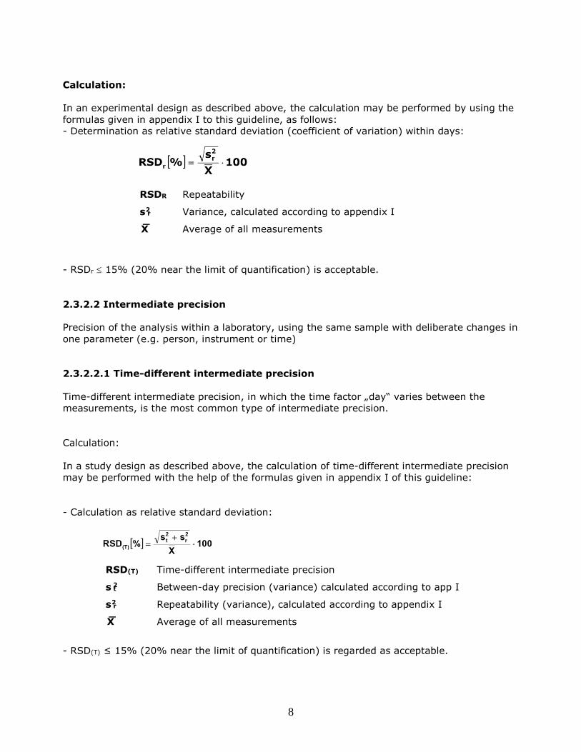
- Determination as relative standard deviation (coefficient of variation) within days:

RSDR Repeatability

s2 r Variance, calculated according to appendix I

X ‾ Average of all measurements

- RSDr 15% (20% near the limit of quantification) is acceptable.

2.3.2.2 Intermediate precision

Precision of the analysis within a laboratory, using the same sample with deliberate changes in

one parameter (e.g. person, instrument or time)

2.3.2.2.1 Time-different intermediate precision

Time-different intermediate precision, in which the time factor „day“ varies between the

measurements, is the most common type of intermediate precision.

Calculation:

In a study design as described above, the calculation of time-different intermediate precision

may be performed with the help of the formulas given in appendix I of this guideline:

- Calculation as relative standard deviation:

RSD(T) Time-different intermediate precision

s 2 t Between-day precision (variance) calculated according to app I

s2 r Repeatability (variance), calculated according to appendix I

X ‾ Average of all measurements

- RSD(T) ≤ 15% (20% near the limit of quantification) is regarded as acceptable.

9

Analogous experimental designs are feasible for the determination of person-different and

instrument-different intermediate precision.

2.3.2.3 Reproducibility, after Ref. [10]

Precision under conditions where results are obtained by using the same method and the same

sample matrix, in different laboratories by different persons using different equipment.

Calculation: Reproducibility cannot be calculated from an experimental design as described

above. It may be determined by analyzing QC samples in different laboratories (e.g. by inter-

laboratory testing, provided all participants use the same analytical protocol).

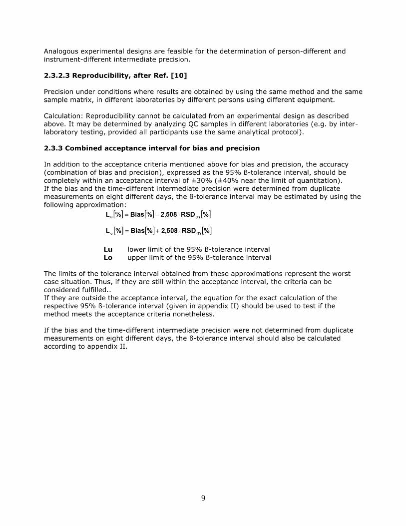
2.3.3 Combined acceptance interval for bias and precision

In addition to the acceptance criteria mentioned above for bias and precision, the accuracy

(combination of bias and precision), expressed as the 95% ß-tolerance interval, should be

completely within an acceptance interval of ±30% (±40% near the limit of quantitation).

If the bias and the time-different intermediate precision were determined from duplicate

measurements on eight different days, the ß-tolerance interval may be estimated by using the

following approximation:

Lu lower limit of the 95% ß-tolerance interval

Lo upper limit of the 95% ß-tolerance interval

The limits of the tolerance interval obtained from these approximations represent the worst

case situation. Thus, if they are still within the acceptance interval, the criteria can be

considered fulfilled..

If they are outside the acceptance interval, the equation for the exact calculation of the

respective 95% ß-tolerance interval (given in appendix II) should be used to test if the

method meets the acceptance criteria nonetheless.

If the bias and the time-different intermediate precision were not determined from duplicate

measurements on eight different days, the ß-tolerance interval should also be calculated

according to appendix II.

10

2.4 Stability, after Ref. [20]

The chemical stability of a substance in a specified matrix under given conditions over given

time intervals.

The stability of the analyte should be warranted from the moment of sampling until the

completion of the analysis. The stability during storage and freezing/thawing is independent of

the analytical method used and therefore appropriate stability data may be taken from the

literature. If these data are not available, they must be acquired during method validation.

In contrast, the stability of the (derivatized) analyte in a processed sample is very much

dependent on the method used. Therefore, it must always be investigated during of method

validation.

2.4.1 Processed sample stability

The stability of the (derivatized) analyte in a completely processed sample in the tray of the

autosampler for the time of a regular analytical batch.

Practical determination:

-Work-up at least 6 QC samples at low and high concentrations (relative to the calibration

range).

-At each concentration, pool the processed samples.

-Divide each sample pool into at least 6 aliquots.

-Inject the aliquots at regular time intervals in over a time period that corresponds to the time

of a regular (routine) analytical batch.

-For each concentration, plot the absolute (!) peak areas (if applicable peak hights) against

the times of injection and apply linear regression.

A significantly negative slope of the regression line indicates instability of the (derivatized)

analyte in processed samples. The maximum acceptable decrease in the peak areas (if

applicable peak hights) over the testing period is 25% when deuterated standards are used

and 15% in other cases (20% near the limit of quantification).

11

2.4.2 Freeze/thaw stability

The stability of the analyte in the sample matrix during repeated freezing and thawing.


-Analyze at least 6 QC samples at low and high concentrations (relative to the calibration

range), without previous treatment (control samples).


range), after at least three freeze/thaw cycles (stability samples).

-Each freeze/thaw cycle should consist of at least 20 hours of freezing and at least 1 hour of

thawing.

The average result of the stability samples should be within 90-110% of the corresponding

average result of the control samples. The 90% confidence interval of the stability samples

should be within 80-120% of the corresponding average value of the control samples.

2.4.3 Long-term stability

The stability of the analyte in the sample matrix during storage over a longer time period.



range), without previous treatment (control samples; they may be the same as the control

samples for freeze/thaw stability)


range), after storage under normal routine storage conditions, preferably over actual storage

periods (stability samples).

The average result of the stability samples should be within 90-110% of the corresponding

average result of the control samples. The 90% confidence interval of the stability samples

should be within 80-120% of the corresponding average value of the control samples.

12

2.5 Analytical limits

2.5.1 Limit of Detection (LOD)

The limit of detection is defined as the lowest concentration of the analyte in a sample, where

the identification criteria are met.

For its estimation, the following methods may be used:

Determination of the signal-to-noise ratio:

-Prepare samples with decreasing analyte concentrations in the range of the expected limit of

detection, by spiking of blank matrix

-Analyze the samples and determine the signal-to-noise ratios.

The limit of detection is the lowest concentration of the analyte in the sample matrix, at which

the signal-to-noise ratio is at least 3:1. In case of MS detection, this applies both to the target

ion and the qualifier ions.

In addition, the identification criteria (see main guideline) must also be met at the LOD.

Alternative for MS-based methods (determination according to DIN 32645 [26]):

-Prepare calibrators at at least 5 concentration levels (not including zero) starting in the range

of the expected LOD by spiking of blank matrix

-Calibrator concentrations should be spaced evenly over the calibration range and the

concentration of the highest calibrator must not be more than 10 times the calculated LOD.

Note: The resulting range of this calibration curve (for the determination of the analytical

limits) is generally not identical with the full calibration- respectively linearity-range of the

method.

-Analyze the calibrators with a number of replicates at each concentration that corresponds to

the number of replicates in routine sample analyses (generally single analysis)

-Plot the peak area ratios (if applicable peak hight ratios; analyte/IS) of the least abundant ion

against the nominal concentrations of the calibrators.

-Apply linear regression and determine the limit of detection by using the following equation

with = 0.01 (in case of GC-MS analyses with = 0.1)

sXO standard deviation of the method

t quantile of the t-distribution

level of significance (error type 1)

m number of measurements

n number of calibration levels

X ‾ content value

Qx sum of quares

13

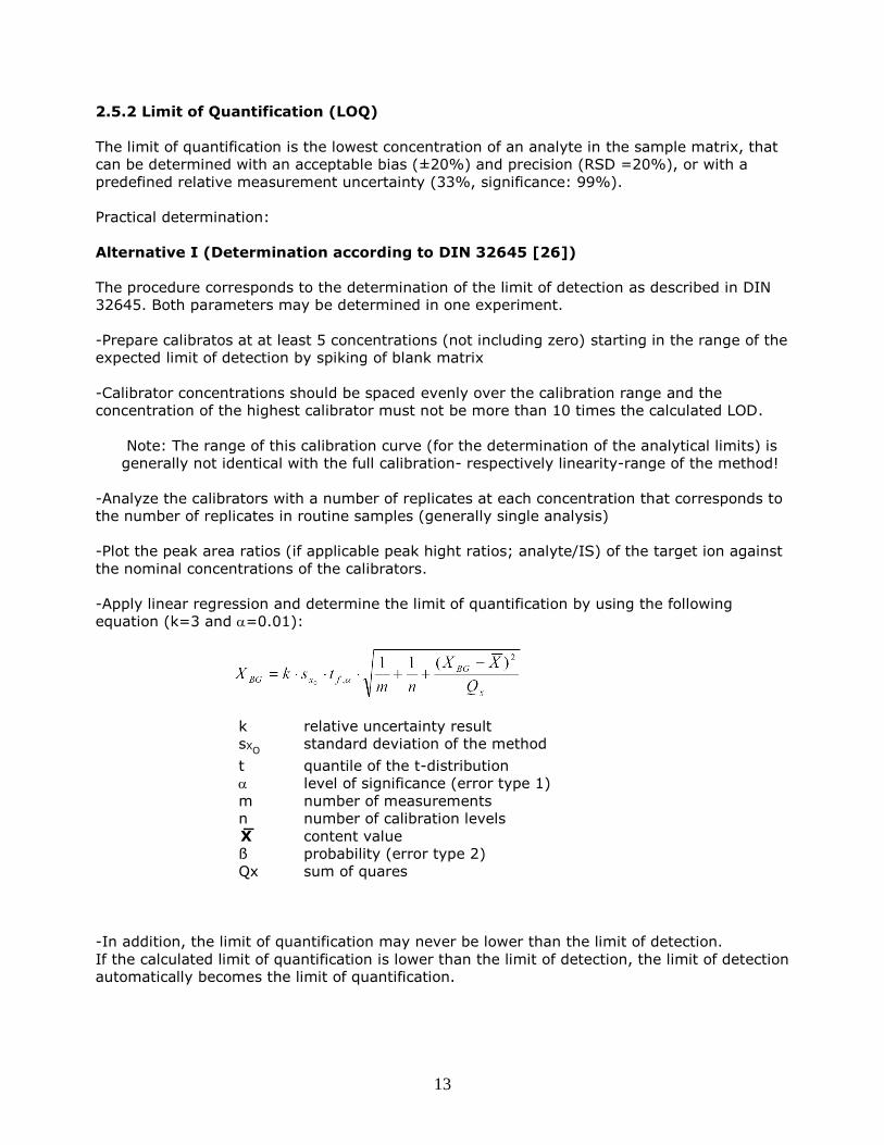
2.5.2 Limit of Quantification (LOQ)

The limit of quantification is the lowest concentration of an analyte in the sample matrix, that

can be determined with an acceptable bias (±20%) and precision (RSD =20%), or with a

predefined relative measurement uncertainty (33%, significance: 99%).


Alternative I (Determination according to DIN 32645 [26])

The procedure corresponds to the determination of the limit of detection as described in DIN

32645. Both parameters may be determined in one experiment.

-Prepare calibratos at at least 5 concentrations (not including zero) starting in the range of the

expected limit of detection by spiking of blank matrix

-Calibrator concentrations should be spaced evenly over the calibration range and the

concentration of the highest calibrator must not be more than 10 times the calculated LOD.

Note: The range of this calibration curve (for the determination of the analytical limits) is

generally not identical with the full calibration- respectively linearity-range of the method!

-Analyze the calibrators with a number of replicates at each concentration that corresponds to

the number of replicates in routine samples (generally single analysis)

-Plot the peak area ratios (if applicable peak hight ratios; analyte/IS) of the target ion against

the nominal concentrations of the calibrators.

-Apply linear regression and determine the limit of quantification by using the following

equation (k=3 and =0.01):

k relative uncertainty result

sXO standard deviation of the method

t quantile of the t-distribution

level of significance (error type 1)

m number of measurements

n number of calibration levels

X ‾ content value

ß probability (error type 2)

Qx sum of quares

-In addition, the limit of quantification may never be lower than the limit of detection.

If the calculated limit of quantification is lower than the limit of detection, the limit of detection

automatically becomes the limit of quantification.

14

Alternative II (Determination by using bias- and precision data) after Ref. [20]

-Prepare a QC sample, independently of the calibrators, with a concentration that corresponds

with that of the lowest calibrator by spiking of blank matrix

-Replicate analysis of the QC sample (at least n=5)

-Determine the bias and repeatability as RSD of the 5 determinations

-The bias should be within ±20% and the RSD 20%

2.6 Recovery and extraction efficiency

2.6.1 Recovery, freely adapted from [12]

The absolute recovery is defined as the complete transfer of the analyte from the matrix into

the final solution to be analysed. It is determined from the ratio of the signals of the same

amount of analyte or standard added to a biological sample and to a neat solution that has not

been extracted (=100%).

The determination of the recovery is always related to the absolute signals measured.

Therefore, it can only be determined for methods, where the substance that is finally

measured is available as pure reference substance.


Alternative I (Determination of the recovery at two concentrations)

-Analyze at least six solutions of neat standard solutions as well as at least six extracts, at

high and low concentrations

-Present the recovery as the ratio of the absolute signals (peak areas or -if applicable- peak

hights) of the extracts to those of the neat standard solutions as a percentage (including

standard deviation or 95% confidence interval)

Alternative II (Determination of the recovery over the entire measuring range)

-Analyze neat standard solutions and extracts at at least six concentrations, spaced evenly

over the measuring range.

-Apply regression analysis of the absolute peak areas (if applicable, peak hights) of extracts

and neat standard solutions over the entire measuring range.

-Report the recovery as the ratio between the slopes of the regression line of the extracts and

the regression line of the neat standard solutions.

15

2.6.2 Extraction efficiency

The extraction efficiency is defined as the integral transfer of an analyte from a matrix into the

primary extract. It is determined from the ratio of the signals of the same amount of analyte

or standard added to a biological sample and to a primary extract of a blank matrix sample

(=100%).

The determination of the extraction efficiency is especially recommended when the method

involves a derivatization step, because the actually measured derivatives are generallynot

available as pure reference standards.


Alternative I (Determination of the extraction efficiency at two concentrations)

-Analyze at least 6 control samples at high and low concentrations respectively, adding the

analyte and the internal standard only after the extraction to the primary extract (100%).

- Analyze at least 6 extracts at high and low concentrations respectively, adding the analyte to

the matrix before the extraction, but adding the internal standard only after the extraction to

the primary extract.

-The extraction efficiency is calculated as the ratio of the peak area ratios (or, if applicable,

the peak hight ratios (analyte/IS)) of the extracts to those of the control samples, as a

percentage including standard deviation or confidence interval (95%)).

Alternative II (Determination of the extraction efficiency over the whole measuring

range)

-Analyze at least 6 control calibrators, evenly spaced over the measuring range, adding the

analyte and the internal standard to the primary extract only after the extraction (100%).

-Analyze at least 6 calibrators, evenly spaced over the measuring range, adding the analyte to

the matrix before the extraction, but adding the internal standard only after the extraction to

the primary extract.

-Apply regresson analysis to the peak area ratios (or, if applicable, the peak hight ratios) of

control calibrators and extracted calibrators

-The extraction efficiency is reported as the ratio of the slopes of the regression lines of the

control calibrators as compared to the extracted calibrators.

The extraction should be reproducible and should have high recoveries repectively high

extraction efficiencies, preferably over 50% corresponding to a slope of 0.5 of the regression

line.

16

2.7 Matrix effects and recovery in LC-MS(/MS) methods

Matrix effects are defined as the direct or indirect change of the absolute ion abundance by the

presence of unintended analytes or other interfering substances in the sample. Both

suppression (ion suppression) and enhancement (ion enhancement) of the signal can occur.


-Analyze at least 5 neat standard solutions at both high and low concentrations (controls).

-Prepare and extract 5 spiked matrix samples at both high and low concentrations using

different blank matrices for each of the 5 samples (spiked matrix samples).

-Prepare 5 spiked blank matrix extracts at both high and low concentrations using the 5

different blank matrices mentioned above (spiked extracts).

-Analyze the controls, the spiked matrix samples and the spiked extracts with LC-MS(/MS).

-Calculate the recovery as the ratio of the peak areas (peak hights if applicable) of the spiked

matrix samples to those of the corresponding spiked extracts as a percentage (average

including standard deviation).

-Calculate the matrix effect as the ratio of the peak areas (peak hights if applicable) of the

spiked extracts to those of the controls as a percentage (average including standard

deviation).

The acceptance criteria for the recovery are the same as specified in paragraph 2.6.2.

The acceptance interval for the average matrix effect is 75-125%. For the standard deviation

of the matrix effect, 25% is acceptable when deuterated internal standards are used, and in

other cases 15% (20% near the limit of quantification).

2.8 Robustness, ruggedness, freely adapted from [20]

The robustness of an analytical method is a measure of its capability to remain unaffected by

small, but deliberate changes in the parameters of the method and shows its reliability under

normal use.

3 Immunochemical methods

The full validation of an immunochemical method is very complex, because of the method-

inhertent nonlinearity of the calibration curves, the decisive influence of the shape of the

calibration curves on the reliability of the positive/negative decision at the cut-off value, and

the susceptibility to unwanted crossreactivities and unspecific binding to matrix components.

The validation is generally performed by the manufacturers for those matrices and cut-off

values that are specified by them. If the immunochemical method is used within these

specifications, a further validation by the user is not necessary. If however the

immunochemical method is not used in accordance with the manufacturer's specifications, e.g.

when using other matrices and/or other cut-off values than proposed by the manufacturer, or

when recommended limits exist for the confirmation analysis, at least the validation

experiments described below should be performed. In case of a large deviation from the

manufacturer's recommendations, a comprehensive validation study can be essential, which

should then be performed in accordance with the guidelines of the US Food and Drug

Administration (FDA) [22].

17

3.1 Selectivity


-Analyze at least 10 blank samples, each from a different batch, with the corresponding

immunochemical method (if applicable after sample pretreatment, e.g. enzymatic hydrolysis,

protein precipitation, extraction, etc)

None of these blanks should give a positive result.

3.2 Adequate Sensitivity

Immunochemical test are used as preliminary tests for the identification of potentially positive

samples. Therefore, positive results should be guaranteed at relevant concentrations of the

relevant target analytes.


-Choose at least 10 authentic samples, for which a concentration in the range of the required

limit of quantification of the confirmatory method has been determined by that method.

-Analyze the samples mentioned above with the immunochemical method (if applicable, after

sample pretreatment, e.g. enzymatic hydrolysis, protein precipitation, extraction, etc).

-In case of a test for a drug group, investigate the relevant target analytes separately.

At least 90% of the cases should give a positive immunochemical result.

18

4 Literature

[1] Peters FT, Drummer OH, Musshoff F (2007) Validation of new methods. For.Sci.Int.

165:216-224.

[2] Bressolle F, Bromet PM, Audran M (1996) Validation of liquid chromatographic and gas

chromatographic methods. Applications to pharmacokinetics. J.Chromatogr.B 686:3-10

[3] Causon R (1997) Validation of chromatographic methods in biomedical analysis. Viewpoint

and discussion. J.Chromatogr.B 689:175-180

[4] Dadgar D, Burnett PE (1995) Issues in evaluation of bioanalytical method selectivity and

drug stability. J.Pharm.Biomed.Anal. 14:23-31

[5] Dadgar D, Burnett PE, Choc MG, Gallicano K, Hooper JW (1995) Application issues in

bioanalytical method validation, sample analysis and data reporting. J.Pharm.Biomed.Anal.

13:89-97

[6] EURACHEM / CITAC. Quantifying Uncertainty in Ananlytical Measurement. 2000.

[7] Hartmann C, Massart DL, McDowall RD (1994) An analysis of the Washington Conference

Report on bioanalytical method validation. J.Pharm.Biomed.Anal. 12:1337-1343

[8] Hartmann C, Smeyers-Verbeke J, Massart DL, McDowall RD (1998) Validation of

bioanalytical chromatographic methods. J.Pharm.Biomed.Anal. 17:193-218

[9] International Conference on Harmonization (ICH). Validation of Analytical Methods:

Definitions and Terminology. ICH Q2 A. 1994.

[10] International Conference on Harmonization (ICH). Validation of Analytical Methods:

Methodology. ICH Q2 B. 1996.

[11] International Organization for Standardization (ISO). Accuracy (Trueness and Precision)

of Measurement Methods and Results. ISO/DIS 5725-1 to 5725-3. 1994.

[12] Karnes HT, Shiu G, Shah VP (1991) Validation of bioanalytical methods. Pharm.Res.

8:421-426

[13] Kromidas S (2000) Validierung in der Analytik. Wiley-VCH, Weinheim

[14] Lindner W, Wainer IW (1998) Requirements for initial assay validation and publication in

J. Chromatography B [editorial]. J.Chromatogr.B 707:1-2

[15] NCCLS (1999) Evaluation of Precision Performance of Chlinical Chemistry Devices;

Approved Guideline. NCCLS, Wayne, PA

[16] Penninckx W, Hartmann C, Massart DL, Smeyers-Verbeke J (1996) Validation of the

Calibration Procedure in Atomic Absorption Spectrometric Methods. J.Anal.At.Spectrom.

11:237-246

[17] Peters FT, Maurer HH (2001) Bioanalytical method validation – How, how much and why?

A review. Toxichem.Krimtech. 68:116-126 (http://www.gtfch.org/tk/tk68_3/Peters.pdf)

19

[18] Peters FT, Maurer HH (2002a) Bioanalytical method validation – How, how much and

why? A review. TIAFT Bulletin 32:16-23

[19] Peters FT, Maurer HH (2002b) Bioanalytical method validation and its implications for

forensic and clinical toxicology - A review. Accred.Qual.Assur. 7:441-449

[20] Shah VP, Midha KK, Dighe S, McGilveray IJ, Skelly JP, Yacobi A, Layloff T, Viswanathan

CT, Cook CE, McDowall RD, Pittman KA, Spector S (1992) Analytical methods validation:

bioavailability, bioequivalence and pharmacokinetic studies. Conference report. Pharm.Res.

9:588-592

[21] Shah VP, Midha KK, Findlay JW, Hill HM, Hulse JD, McGilveray IJ, McKay G, Miller KJ,

Patnaik RN, Powell ML, Tonelli A, Viswanathan CT, Yacobi A (2000) Bioanalytical method

validation- a revisit with a decade of progress. Pharm.Res. 17:1551-1557

[22] U.S.Department of Health and Human Services, Food and Drug Administration. Guidance

for Industry, Bioanalytical Method Validation. 2001.

http://www.fda.gov/CDER/GUIDANCE/4252fnl.pdf

[23] Vander-Heyden Y., Nijhuis A, Smeyers-Verbeke J, Vandeginste BG, Massart DL (2001)

Guidance for robustness/ruggedness tests in method validation. J Pharm Biomed Anal 24:723-

753

[24] Wieling J, Hendriks G, Tamminga WJ, Hempenius J, Mensink CK, Oosterhuis B, Jonkman

JH (1996). Rational experimental design for bioanalytical methods validation. Illustration using

an assay method for total captopril in plasma. J.Chromatogr.A 730:381-394

[25] Hubert Ph, Nguyen-Huu J-J, Boulanger B, Chapuzet E, Cohen N, Compagnon P-A, Dewe

W, Feinberg M, Laurentie M, Mercier N, Muzard G, Valat L, Rozet E (2007) Harmonization of

strategies for the validation of quantitative analytical procedures, A SFSTP Proposal - Part III.

J.Pharm.Biomed.Anal. 45:82-96

[26] DIN EN ISO/IEC 32645:1994

5 Date of approval

This appendix was approved by decision of the Board of the GTFCh on April 1, 2009 and has

come into force after publication in "Toxichem + Krimtech".

Transitional terms apply until March 31, 2011.

20

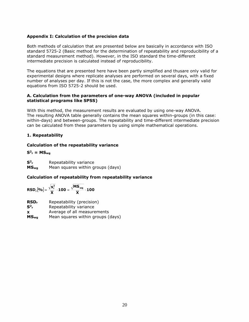
Appendix I: Calculation of the precision data

Both methods of calculation that are presented below are basically in accordance with ISO

standard 5725-2 (Basic method for the determination of repeatability and reproducibility of a

standard measurement method). However, in the ISO standard the time-different

intermediate precision is calculated instead of reproducibility.

The equations that are presented here have been partly simplified and thusare only valid for

experimental designs where replicate analyses are performed on several days, with a fixed

number of analyses per day. If this is not the case, the more complex and generally valid

equations from ISO 5725-2 should be used.

A. Calculation from the parameters of one-way ANOVA (included in popular

statistical programs like SPSS)

With this method, the measurement results are evaluated by using one-way ANOVA.

The resulting ANOVA table generally contains the mean squares within-groups (in this case:

within-days) and between-groups. The repeatability and time-different intermediate precision

can be calculated from these parameters by using simple mathematical operations.

1. Repeatability

Calculation of the repeatability variance

S2r = MSwg

S2r Repeatability variance

MSwg Mean squares within groups (days)

Calculation of repeatability from repeatability variance

RSDr Repeatability (precision)




21

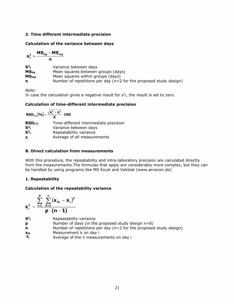
2. Time different intermediate precision

Calculation of the variance between days

S2t Variance between days

MSbg Mean squares between groups (days)


n Number of repetitions per day (n=2 for the proposed study design)

Note:

In case the calculation gives a negative result for s2t, the result is set to zero.

Calculation of time-different intermediate precision

RSD(T) Time-different intermediate precision




B. Direct calculation from measurements

With this procedure, the repeatability and intra-laboratory precision are calculated directly

from the measurements.The formulas that apply are considerably more complex, but they can

be handled by using programs like MS Excel and Valistat (www.arvecon.de).

1. Repeatability

Calculation of the repeatability variance


p Number of days (in the proposed study design n=8)


xik Measurement k on day i

Average of the n measurements on day i

22

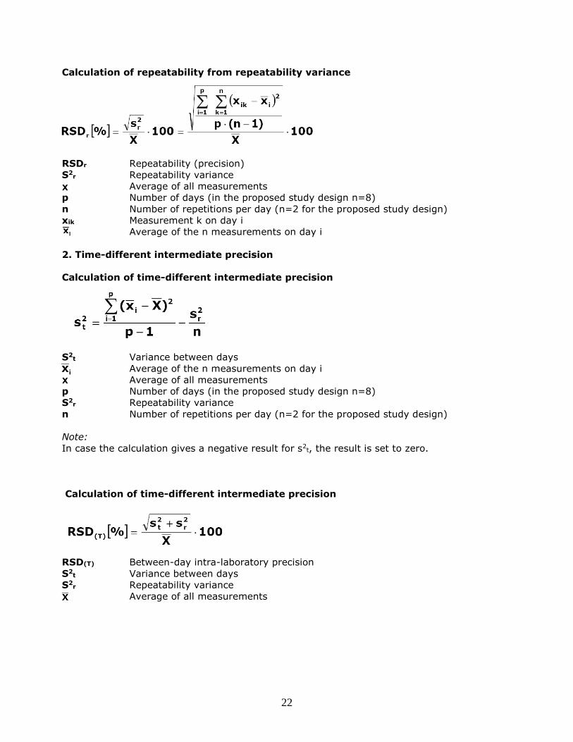
Calculation of repeatability from repeatability variance

RSDr Repeatability (precision)





xik Measurement k on day i


2. Time-different intermediate precision








Note:

In case the calculation gives a negative result for s2t, the result is set to zero.


RSD(T) Between-day intra-laboratory precision




23

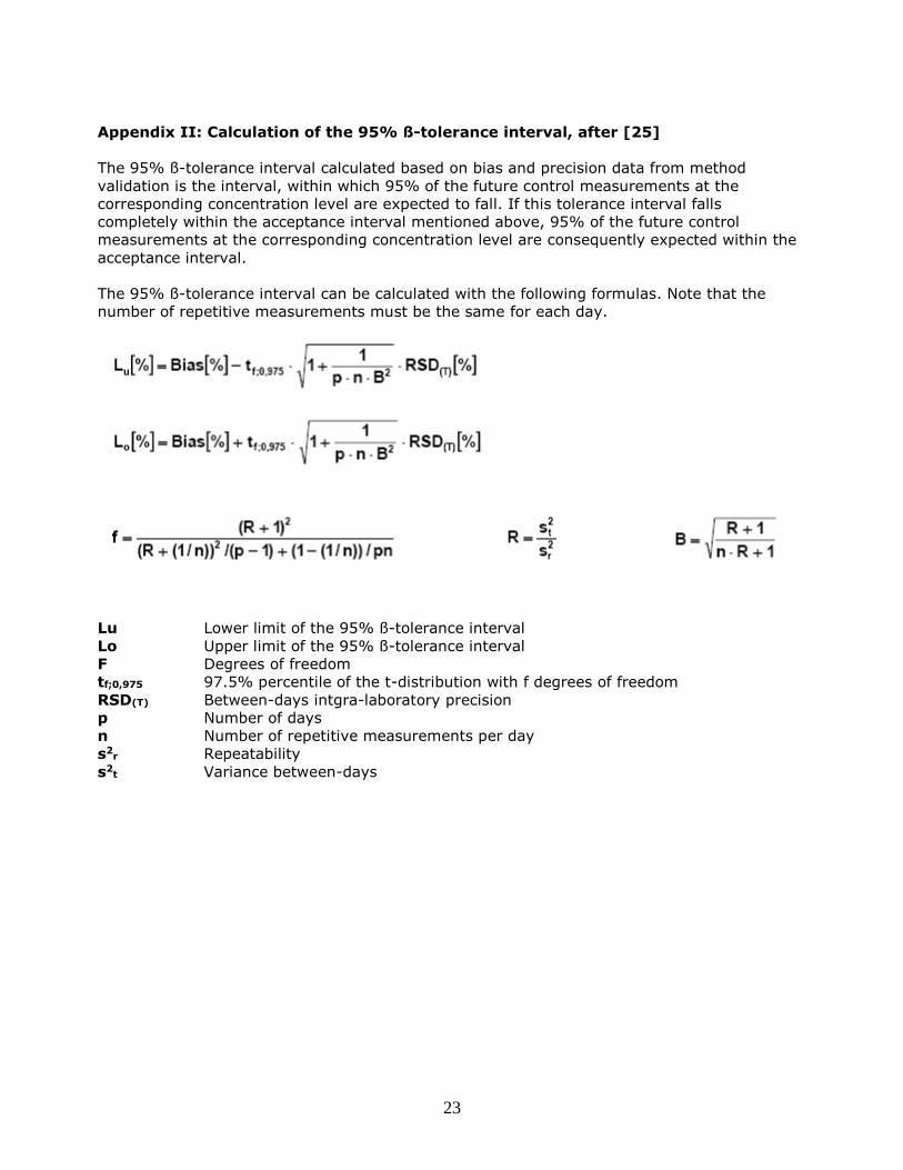
Appendix II: Calculation of the 95% ß-tolerance interval, after [25]

The 95% ß-tolerance interval calculated based on bias and precision data from method

validation is the interval, within which 95% of the future control measurements at the

corresponding concentration level are expected to fall. If this tolerance interval falls

completely within the acceptance interval mentioned above, 95% of the future control

measurements at the corresponding concentration level are consequently expected within the

acceptance interval.

The 95% ß-tolerance interval can be calculated with the following formulas. Note that the

number of repetitive measurements must be the same for each day.

Lu Lower limit of the 95% ß-tolerance interval

Lo Upper limit of the 95% ß-tolerance interval

F Degrees of freedom

tf;0,975 97.5% percentile of the t-distribution with f degrees of freedom

RSD(T) Between-days intgra-laboratory precision

p Number of days

n Number of repetitive measurements per day

s2r Repeatability

s2t Variance between-days

requirements for the validation of analytical methods b gtfch... · 3 1 introduction the validation...

Documents