representation and diurnal variation of upper ... -...
TRANSCRIPT
DOCTORA L T H E S I S
Department of Computer Science, Electrical and Space EngineeringDivision of Space Technology
Representation and Diurnal Variation of Upper Tropospheric Humidity in
Observations and Models
Ajil Kottayil
ISSN: 1402-1544ISBN 978-91-7439-604-1 (tryckt)ISBN 978-91-7439-605-8 (pdf)
Luleå University of Technology 2013
Ajil K
ottayil Representation and D
iurnal Variation of Upper T
ropospheric Hum
idity in Observations and M
odels
ISSN: 1402-1544 ISBN 978-91-7439-XXX-X Se i listan och fyll i siffror där kryssen är


PhD thesis
Representation and Diurnal Variation of
Upper Tropospheric Humidity in
Observations and Models
Ajil Kottayil
29 April 2013
Department of Computer Science, Electrical and Space EngineeringDivision of Space TechnologyLulea University of Technology
Kiruna, Sweden

Printed by Universitetstryckeriet, Luleå 2013
ISSN: 1402-1544 ISBN 978-91-7439-604-1 (tryckt)ISBN 978-91-7439-605-8 (pdf)
Luleå 2013
www.ltu.se

To Rosh...


Abstract
The role of water vapour is manifold in its climate regulation of the Earth system.Most important of all despite its low concentration, is the role it plays in the uppertroposphere. It assumes an important role in its contribution to greenhouse warmingby way of its positive feedback effect, amplifying the radiative forcing due to increasingCO2 concentrations. Understanding the variability and distribution is thus importantfrom a climate point of view and critical because the challenges involved in it are fartoo many. This thesis consists of an introduction and three research articles focusingon the study of upper tropospheric humidity (UTH). The first two articles are ontwo important sources of UTH data, the radiosondes and satellite data, and the thirdis associated with climate models, important tools for simulating and reproducingglobal climate features. The summaries of these three articles are as follows:
Radiosondes have been the primary sources for vertical profiles of various atmo-spheric parameters and are one of the crucial components in numerical weather pre-dictions and satellite validations. However, they are known to have certain issues withmeasurements of humidity in the upper troposphere. The first article highlights theimportance of radiosonde humidity corrections by using satellite measurements as thereference. The infrared and microwave measurements from NOAA-17 polar orbitingsatellite were used as the reference in this study. Collocated radiosonde measurementsfrom the Atmospheric Radiation Measurement (ARM) campaign were converted intosatellite radiances using the ARTS radiative transfer model. The comparisons withsatellite measurements were done separately for daytime and nighttime soundings ofradiosonde under clear sky conditions. An empirical correction procedure meant toaddress the mean bias error and solar radiation error was applied to the radiosondes.The empirical correction was found to significantly reduce the dry bias of radiosondesin the upper troposphere. The impact of the correction is prominent over daytimeradiosonde measurements on account of the bias removal associated with the solarradiation error.
Long term time-series measurements of tropospheric humidity are available frompolar orbiting satellites but the measurements from these satellites have been foundto be affected by diurnal sampling bias, which is caused by a drift in the orbital heightof the satellites, thus changing the local sampling time of the satellites over course oftime. This therefore introduces a spurious trend into the time-series data obtainedfrom these satellites. A methodology for the correction of orbital drift error appliedon microwave humidity measurements from NOAA and MetOpA satellites forms thesubject of the second article included in this thesis. Climatological diurnal cycles
v

of microwave humidity measurements were obtained from 5 different polar orbitingsatellites to infer and thereby correct the diurnal sampling bias in microwave humiditymeasurements. The diurnal cycles were generated separately for the 5 microwavechannels. A Monte Carlo error analysis also determines the significance of diurnalamplitudes. The impact of diurnal correction has been evaluated by analyzing thesurface channel brightness temperature time-series of NOAA-16 and UTH channeltime-series of NOAA-17 satellites. The impact of diurnal correction is greater for thesurface channels when compared to the UTH channels due to the larger diurnal cycleamplitudes in the surface channels.
Climate models are one of the main tools for the prediction of future climatechange. Most processes associated with water vapour appear in climate models asparameterizations since they are too small-scale or complex to be physically repre-sented in models. Therefore, frequent validation of models against observations isneeded to assure their reliability. The third article evaluates the performance of twoclimate models, in simulating the diurnal cycles of upper tropospheric humidity tak-ing combined microwave humidity measurements from four different satellites as thereference. The comparisons were made over the convective land and oceanic regionsover the tropics. The diurnal cycle differences between infrared and microwave ob-servations and the reason for these differences are also analyzed. It is shown thatthe cloud sensitivity differences in infrared data can shift the diurnal phase relativeto microwave data. The models exhibit considerable differences in the diurnal phaseand amplitude of UTH as against microwave observations over both land and oceanicregions.
Appended papers
• Paper I:Kottayil. A., S. A. Buehler, V. O. John, L. M. Miloshevich, M. Milz, and G.Holl (2012), On the importance of Vaisala RS92 radiosonde humidity correctionsfor a better agreement between measured and modeled satellite radiances, J.Atmos. Oceanic Technol., 29, 248259, doi:10.1175/JTECH-D-11-00080.1.
• Paper II:Kottayil, A., V. O. John, and S. A. Buehler (2013), Correcting diurnal cyclealiasing in satellite microwave humidity sounder measurements, J. Geophys.Res., 118(1), 101113, doi:10.1029/2012JD018545.
• Paper III:Kottayil, A., S. A. Buehler, and V. O. John (under revision, 2013), Evaluatingthe diurnal cycle of upper tropospheric humidity in two different climate modelsusing satellite observations, J. Geophys. Res.
vii


Related papers
• Holl. G., S. A. Buehler, J. Mendrok, and A. Kottayil (2012), Optimisedfrequency grids for infrared radiative transfer simulations in cloudy conditions,J. Quant. Spectrosc. Radiat. Transfer, doi:10.1016/j.jqsrt.2012.05.022.
• Thapliyal, P. K., M. V. Shukla, S. Shah, P. K. Pal, P. C. Joshi, andA. Kottayil(2011), An algorithm for the estimation of upper tropospheric humidity fromKalpana observations: Methodology and validation, J. Geophys. Res., 116, 116,doi:doi:10.1029/2010JD014291.
• Kottayil, A., P. K. Thapliyal, M. V. Shukla, P. K. Pal, P. C. Joshi, and R.R. Navalgund (2010), A new technique for temperature and humidity profileretrieval from infrared sounder observations using Adaptive Neuro-Fuzzy Infer-ence System, IEEE Geosci. Remote Sens., 48, 1650 –1655.
• V. O. John, R. P. Allen, W. Bell, S. A. Buehler and A. Kottayil (in press,2013), Assessment of inter-calibration methods for satellite microwave humiditysounders, J. Geophys. Res.
• Buehler, S. A., V. O. John, A. Kottayil, M. Milz, and P. Eriksson (2010),Efficient Radiative Transfer Simulations for a Broadband Infrared Radiome-ter Combining a Weighted Mean of Representative Frequencies Approach withFrequency Selection by Simulated Annealing, J. Quant. Spectrosc. Radiat.Transfer, 111(4), 602615, doi:10.1016/j.jqsrt.2009.10.018.
ix

Contents
Abstract iii
Appended papers vii
Related papers ix
Table of contents xi
List of figures xiii
Acknowledgements xv
Preface xvii
Chapter 1 – Introduction 1
1.1 Introduction . . . . . . . . . . . . . . . . . . . . . . . . . . . . . . . . 1
1.2 Radiative Forcing and Feedback Processes . . . . . . . . . . . . . . . 2
1.3 Satellite Remote Sensing of UTH . . . . . . . . . . . . . . . . . . . . 6
1.3.1 Microwave Humidity Sounders . . . . . . . . . . . . . . . . . . 8
1.3.2 HIRS . . . . . . . . . . . . . . . . . . . . . . . . . . . . . . . . 8
1.4 UTH in Climate Models . . . . . . . . . . . . . . . . . . . . . . . . . 10
1.5 Aim of the Thesis . . . . . . . . . . . . . . . . . . . . . . . . . . . . . 14
1.6 Thesis Outline . . . . . . . . . . . . . . . . . . . . . . . . . . . . . . . 14
Chapter 2 – Radiative Transfer 17
2.1 Radiation Laws . . . . . . . . . . . . . . . . . . . . . . . . . . . . . . 17
2.2 Clear Sky Radiative Transfer Equation . . . . . . . . . . . . . . . . . 19
2.3 ARTS . . . . . . . . . . . . . . . . . . . . . . . . . . . . . . . . . . . 21
Chapter 3 – Radiosonde Corrections 25
3.1 Radiosonde Correction Methods . . . . . . . . . . . . . . . . . . . . . 26
3.1.1 Mean Calibration Bias Correction . . . . . . . . . . . . . . . . 26
3.1.2 Solar Radiation Error Correction . . . . . . . . . . . . . . . . 27
3.1.3 Time Lag Correction . . . . . . . . . . . . . . . . . . . . . . . 28
xi
Chapter 4 – Summary of Papers 314.1 Paper I . . . . . . . . . . . . . . . . . . . . . . . . . . . . . . . . . . . 314.2 Paper II . . . . . . . . . . . . . . . . . . . . . . . . . . . . . . . . . . 324.3 Paper III . . . . . . . . . . . . . . . . . . . . . . . . . . . . . . . . . . 32
Chapter 5 – Conclusions and Future Work 35
References 37
Glossary 43
Acronyms 43
Acronyms 43
Paper I 45
Paper II 59
Paper III 75
List of figures
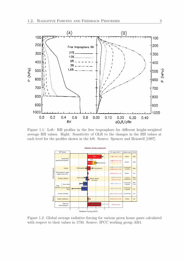
1.1 Left: RH profiles in the free troposphere for different height-weightedaverage RH values. Right: Sensitivity of OLR to the changes in the RHvalues at each level for the profiles shown in the left. Source: Spencerand Braswell [1997]. . . . . . . . . . . . . . . . . . . . . . . . . . . . . 3
1.2 Global average radiative forcing for various green house gases calcu-lated with respect to their values in 1750. Source: IntergovernmentalPanel on Climate Change (IPCC) working group 4th Assessment Re-port (AR4). . . . . . . . . . . . . . . . . . . . . . . . . . . . . . . . . 3
1.3 Water vapour kernel from the different parts of the troposphere fordifferent latitude bands. The unit of water vapour kernel is W m−2
K−1 /100 hPa. Source: Soden and Held [2006] . . . . . . . . . . . . . 5
1.4 Relationship between surface temperature and precipitable water. Source:[Gaffen et al., 1992]. . . . . . . . . . . . . . . . . . . . . . . . . . . . 5
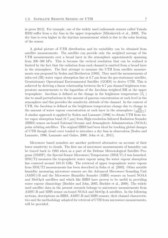
1.5 Atmospheric opacity for the FASCOD midlatitude summer scenario forH2O (dashed), O2 (dotted), N2 (dash dotted), and O3 (solid). The longdashed line represents the total opacity. Shaded regions represent thepassband positions of AMSU-B channels. Source: John and Buehler[2004]. . . . . . . . . . . . . . . . . . . . . . . . . . . . . . . . . . . . 9
1.6 Water vapour Jacobian for AMSU-B channels for a standard tropicalprofile. . . . . . . . . . . . . . . . . . . . . . . . . . . . . . . . . . . . 10
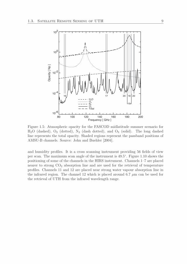
1.7 Relationship between UTH and channel 18 brightness temperature fornadir view of the NOAA and MetOpA satellites. Source: Buehler andJohn [2005]. . . . . . . . . . . . . . . . . . . . . . . . . . . . . . . . . 11
1.8 Distribution of UTH mean value for the month of July 2007 retrievedfrom NOAA-17 satellite from 183.31±1.00 water vapour absorptionline. The unit is in %RH. . . . . . . . . . . . . . . . . . . . . . . . . 11
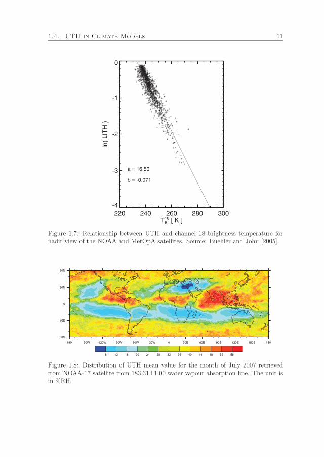
1.9 Clear sky bias in the infrared estimates of UTH for the month of July.Bias is defined as the difference between infrared sampled and mi-crowave sampled UTH. Source: John et al. [2011] . . . . . . . . . . . 12
xiii

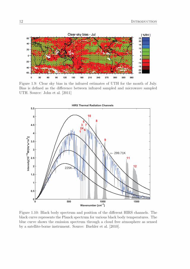
1.10 Black body spectrum and position of the different HIRS channels. Theblack curve represents the Planck spectrum for various black bodytemperatures. The blue curve shows the emission spectrum througha cloud free atmosphere as sensed by a satellite-borne instrument.Source: Buehler et al. [2010]. . . . . . . . . . . . . . . . . . . . . . . . 12
2.1 Azimuth angle (ψ), zenith angle(θ) and solid angle as related to a unithemisphere. Source: Modest [2003]. . . . . . . . . . . . . . . . . . . . 18
2.2 Transmission of radiation through atmosphere. . . . . . . . . . . . . . 222.3 Absorption line shape associated with Doppler broadening and pressure
broadening. Source: Wallace and Hobbs [2006]. . . . . . . . . . . . . 222.4 Water vapour Jacobians for AMSU-B channels 18,19 and 20. The
upper and lower panels represent moist tropical atmosphere and drymid latitude winter atmosphere, respectively. Simulations for nadirand off nadir views of the instrument are indicated as solid and dottedlines, respectively. Source: John [2005]. . . . . . . . . . . . . . . . . . 23
3.1 The Vaisala RS92 mean bias curve. Source: Miloshevich et al. [2009] 273.2 Polynomial coefficients provided for mean bias correction for day and
nighttime RS92 radiosonde profiles. Source: Miloshevich et al. [2009] 273.3 Solar fraction error as the function of solar altitude angle. Source:
Miloshevich et al. [2009] . . . . . . . . . . . . . . . . . . . . . . . . . 293.4 RS92 time constant as a function of temperature. Source: http://
milo-scientific.com/prof/radiosonde.php. . . . . . . . . . . . . 30

Acknowledgements
“We are each of us angels with only one wing and we can fly only byembracing one another ” - Luciano de Crescenzo
Its been 4 years and 5 months since I first set foot on this sub-arctic frozen townof Kiruna for my doctoral research. My research journey has been very enrichingand it is with a deep sense of appreciation and gratitude for the many good peoplein my life that I pen this note of acknowledgment. I am deeply indebted to Prof.Dr. Stefan Buehler, my supervisor for his constant support and guidance throughoutmy research. Even though his criticisms sometimes have caused a slight pressure, Ihave always realized eventually that they greatly improve the quality of my work. Iwould also like to thank Dr. Viju John, my co-supervisor, a fellow countryman anda good friend, for his constant support and help on scientific matters. I have alwaysfound him an open person, ready to help and always encouraging. Many thanks toLarry Miloschevich for productive scientific discussions and Andrew Gettelman forproviding the CAM5 model output and for valuable comments on the manuscript.Thanks to Dr. Prince Xavier for helping in the GA-3 model run.
It has been a privilege to work in a group with very supportive peers. I amobliged to each and every member of the SAT group for the many favors I havereceived from them. Thank you Gerrit Holl, Salomon Eliasson, Isaac Moradi, JanaMendrok, Mathias Milz, Thomas Kuhn, Anura Wickramanayake, Madhuri Nukala,Oscar Isoz and Richard Larsson. I owe a special thanks to Oliver Lemke for all histechnical help and support. I would also like to mention my gratefulness towards Dr.Victoria Barabash, Maria Winneback, Anette Brandstrom and Lars Jakobsson forassisting me in the administrative procedures. I enjoy a warm camaraderie with myfellow PhD group at IRF and I wish to convey my deep regards to Rikard, Maria. S,Catherine, Maria. M, Katarina, Shahab and Charles. I would also like to thank theGraduate School of Space Technology for their academic support.
I recall with gratefulness Satheesan Karathazhiyath who was of great help tome when I first came to Kiruna. Thanks to him, I never had to face the pain ofacclimatizing to the new place and its ways. I had my first skiing lessons from JonasEkeberg and I take this opportunity to thank him for the wonderful time I had with hisfamily on a Christmas Eve. Back in India, I am fortunate to have some good friends,mentors and well-wishers. I thank Dr. P. K. Thapliyal who not only introduced meto satellite remote sensing but also went on to inspire me into taking it up as myresearch interest. For whatever I have made of myself today and wherever I am to
xv

go from here, I would always be indebted to Dr. Sabukutty, my biggest mentor andguide. A special thanks to Dr. Sathiyamoorthy who motivated me to apply for thisparticular PhD position.
I thank all my dear friends Rakesh, Rajkumar Kamaljith, Imran Ali, NaveenShahi, Vishal, Mahesh, Remya, Jidesh, Harsh, Prince, Rahul, Munn Vinayak, Thomas,Ravish, Anoop. G, Satya Prakash, Sanjeev for their lively companionship. I now re-serve this space to acknowledge my family, my parents and my sister whose moralsupport, love and sacrifices have always motivated me to strive for betterment. Per-haps this space will not suffice for acknowledging every one of whom I have been abeneficiary and any omission in this brief acknowledgement does not mean lack ofgratitude.

Preface
This thesis is an expanded version of the Licentiate thesis defended in 2012 as a re-quirement for the Licentiate degree in Space Technology [Kottayil, 2012]. In Sweden,the Licentiate degree is an intermediate postgraduate degree prior to PhD and is anacademic step achieved normally towards half the tenure of PhD research. Certainparts of the section 2.2 of the Chapter 2 included in this thesis has been taken fromthe Chapter 2 of the licentiate thesis. Most of the materials included in Chapter 3of this thesis have been taken from Chapter 4 of the Licentiate thesis but this hasbeen augmented with more information. One paper (Paper-I) which was a part ofthe Licentiate thesis is also appended here as a part of this PhD thesis.
xvii


Chapter 1
Introduction
1.1 Introduction
The increasing awareness of a changing climate and the role played in it by watervapour has elevated the interest of water vapour related studies in atmospheric sci-ence. Water vapour is the most important contributor to the natural greenhouseeffect and is highly variable in space and time. One of the fundamental approxima-tions governing the atmospheric thermodynamics is given by the Clausius-Clapeyronequation which explains the dependence of atmospheric saturated moisture contenton the air temperature [Allan, 2012]:
1
qs
dqsdT
≈ 1
es
desdT
=L
RvT 2(1.1)
where qs is the saturation specific humidity; the ratio of the mass of water vapor inair to the total mass of the mixture of air and water vapor (kg/kg), es is the satura-tion water vapour pressure (Pa), T is the air temperature (K), L is the latent heatof vapourisation (2.59 × 10⁶ Jkg−1), Rv is the gas constant for water vapour (461JK−1kg−1). Under the assumption of fixed Relative Humidity (RH), the Equation1.1 predicts a 6–7%/K change in the specific humidity, for temperatures close to thesurface. From model simulations, Held and Soden [2006] found a 7.5%/K increasein the global mean water vapour relative to global surface temperature change cor-roborating the values predicted by Equation 1.1 and supporting the notion of aninvariant RH. Trenberth et al. [2005] have also shown a fractional increase in thelower tropospheric humidity with respect to the surface temperature changes in theorder of 7.8 %/K from satellite measurements, which again supports the assumptionof constant RH. As the Earth’s atmosphere gets warmer due to enhanced emission ofgreen house gases (GHG), its water vapour concentration increases exponentially withtemperature (From Equation 1.1). Since water vapour is a strong infrared absorber,an increased amount of water vapour therefore absorbs more radiation resulting in
1
2 Introduction
an even warmer atmosphere.The global warming is now a phenomenon existing beyond any doubt and there is
indeed a steady increase in global temperatures over the past few decades [Hansen andLebedeff, 1987]. The monitoring of Upper Tropospheric Humidity (UTH) in a scenarioof changing climate plays a central role in the prediction of future climate which islargely because of its sensitivity to Outgoing Longwave Radition (OLR). Therefore,relatively small fluctuations in amount water vapour in the free troposphere will havea great influence on the radiation budget [Kiehl and Briegleb, 1992, Held and Soden,2000]. The changes in the clear sky OLR to the upper tropospheric humidity changesare even larger for dry subsidence regions as compared to moist regions and it has beenshown that the impact of humidity fluctuations on OLR is almost threefold at 10% RHas compared to humidity fluctuations at 90% RH [Spencer and Braswell, 1997]. Theanalysis of long term time series of satellite measurements by Soden et al. [2005] couldnot demonstrate any trend in the upper tropospheric RH, thus implying an increasein the specific humidity in the upper troposphere. The upper tropospheric moisteningshown by Soden et al. [2005] also agrees with the climate model projections. However,a better picture of water vapour distribution, its trends over time and how variousatmospheric processes are affected by it, are yet to be gained from scientific studies[Sherwood et al., 2010]. A direct step towards this would be to make available thewater vapour concentration from all parts of the atmosphere and from all regions.
1.2 Radiative Forcing and Feedback Processes
The Earth receives solar energy and gets heated up and in return, it emits radiationin the infrared range of the electromagnetic spectrum. The Earth’s energy budget atthe Top of Atmosphere (TOA) is given by
R = (So/4)(1− α)−OLR (1.2)
where So, α and OLR are the insolation, the planetary albedo, and the TOA OLR.The radiative forcing refers to the imbalance between the energy received by the Earthand the energy re-radiated by the Earth into the space. Depending on whether thesystem gets warmer on account of greater incoming radiation or the system gets coolerowing to more outgoing energy, this forcing could be termed positive or negative. Thisradiative forcing occurs due to changes in the solar insolation and the variability inthe concentrations of GHGs and aerosols. The IPCC report of 2007 cites increases inGHG concentrations in the order of 150% in methane, 18% in nitrous oxide and 38%in CO2 between the period of 1750 and 2005. The radiative forcing due to differentatmospheric constituents is summarized in Figure 1.2.
For instance, external perturbations such as changes in the atmospheric concen-trations of CO2, or changes in the solar constant when introduced into the climatesystem, bring a difference in the Earth’s radiation budget by ΔQ. The climate systemresponds to this radiative forcing by changes in its global mean surface temperature.As given in Bony et al. [2006], the change in the global mean surface temperature ΔTs
1.2. Radiative Forcing and Feedback Processes 3
Figure 1.1: Left: RH profiles in the free troposphere for different height-weightedaverage RH values. Right: Sensitivity of OLR to the changes in the RH values ateach level for the profiles shown in the left. Source: Spencer and Braswell [1997].
Radiative forcing components
Figure 1.2: Global average radiative forcing for various green house gases calculatedwith respect to their values in 1750. Source: IPCC working group AR4.

4 Introduction
is related to this radiative forcing and to the radiative imbalance in TOA through theequation:
ΔR = ΔQ+ λΔTs (1.3)
where λ is called the feedback parameter. The climate system attains a new equilib-rium when ΔR =0. At equilibrium,
ΔQ = −λΔTs (1.4)
As a first order approximation by neglecting the interaction between various com-ponents in the climate system, the feedback parameter λ can be written as [Bonyet al., 2006]:
λ =∂R
∂Ts+∑xi
∂R
∂x
∂x
∂Ts(1.5)
The first term of the Equation 1.5 denotes the black body feedback parameter(λo), and this gives the differences in the TOA energy balance due to changes in thesurface temperature in response to an external radiative forcing. This feedback canbe calculated as
∂R
∂Ts= −4σT 3
s (1.6)
where σ = 5.6 × 10⁻⁸ W m−2 K−4 is the Stefan-Boltzman constant. Assuming anemission temperature of 255 K, this value is close to -3.78 W m−2 K−1. The secondterm in the Equation 1.5 represents the feedback variables such as water vapour, cloud,surface albedo etc. Therefore, the feedback λ in Equation 1.5 can be decomposed intofeedback related to temperature, water vapour, cloud and surface albedo. The watervapour feedback parameter can be written as [Bony et al., 2006]:
λw =∂R
∂q
∂q
∂Ts(1.7)
The first term (∂R∂q) in the equation relates to radiative transfer and can be deter-
mined from model outputs by introducing a perturbation of humidity at the surface.The resulting change in the TOA flux can be used to determine ∂R
∂q. The second
term can be determined from water vapour–surface temperature relationship as inFigure 1.4. While calculating the actual temperature and water vapour feedback, itis necessary to introduce temperature and water vapour perturbations in differentlayers of the troposphere and then observe the change in the TOA flux, as differentphysical processes control the feedback response in these different layers [Soden andHeld, 2006, Soden et al., 2008]. Figure 1.3 shows the ’water vapour kernel’, a nomen-clature adopted for ∂R
∂qas in Soden and Held [2006]. Based on the estimates from
model simulation as in Colman [2003] and Soden and Held [2006], the value of λo isestimated to be about -3.2 W m−2 K−1. The water vapour feedback value λw deducedfrom climate model simulation is about +1.8 W m−2 K−1 [Soden and Held, 2006].

1.2. Radiative Forcing and Feedback Processes 5
Figure 1.3: Water vapour kernel from the different parts of the troposphere for differ-ent latitude bands. The unit of water vapour kernel is W m−2 K−1 /100 hPa. Source:Soden and Held [2006]
Figure 1.4: Relationship between surface temperature and precipitable water. Source:[Gaffen et al., 1992].
6 Introduction
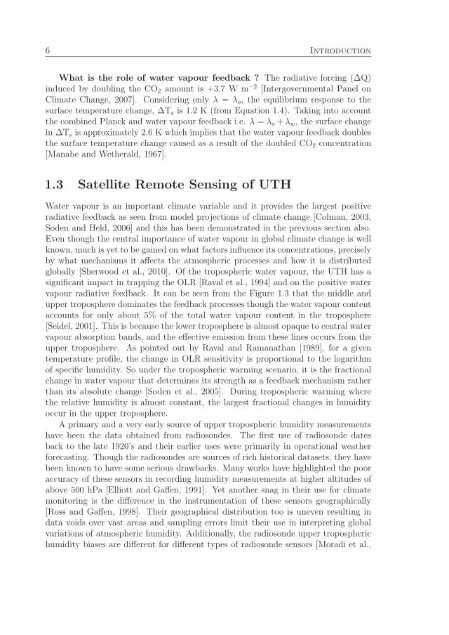
What is the role of water vapour feedback ? The radiative forcing (ΔQ)induced by doubling the CO2 amount is +3.7 W m−2 [Intergovernmental Panel onClimate Change, 2007]. Considering only λ = λo, the equilibrium response to thesurface temperature change, ΔTs is 1.2 K (from Equation 1.4). Taking into accountthe combined Planck and water vapour feedback i.e. λ = λo +λw, the surface changein ΔTs is approximately 2.6 K which implies that the water vapour feedback doublesthe surface temperature change caused as a result of the doubled CO2 concentration[Manabe and Wetherald, 1967].
1.3 Satellite Remote Sensing of UTH
Water vapour is an important climate variable and it provides the largest positiveradiative feedback as seen from model projections of climate change [Colman, 2003,Soden and Held, 2006] and this has been demonstrated in the previous section also.Even though the central importance of water vapour in global climate change is wellknown, much is yet to be gained on what factors influence its concentrations, preciselyby what mechanisms it affects the atmospheric processes and how it is distributedglobally [Sherwood et al., 2010]. Of the tropospheric water vapour, the UTH has asignificant impact in trapping the OLR [Raval et al., 1994] and on the positive watervapour radiative feedback. It can be seen from the Figure 1.3 that the middle andupper troposphere dominates the feedback processes though the water vapour contentaccounts for only about 5% of the total water vapour content in the troposphere[Seidel, 2001]. This is because the lower troposphere is almost opaque to central watervapour absorption bands, and the effective emission from these lines occurs from theupper troposphere. As pointed out by Raval and Ramanathan [1989], for a giventemperature profile, the change in OLR sensitivity is proportional to the logarithmof specific humidity. So under the tropospheric warming scenario, it is the fractionalchange in water vapour that determines its strength as a feedback mechanism ratherthan its absolute change [Soden et al., 2005]. During tropospheric warming wherethe relative humidity is almost constant, the largest fractional changes in humidityoccur in the upper troposphere.
A primary and a very early source of upper tropospheric humidity measurementshave been the data obtained from radiosondes. The first use of radiosonde datesback to the late 1920’s and their earlier uses were primarily in operational weatherforecasting. Though the radiosondes are sources of rich historical datasets, they havebeen known to have some serious drawbacks. Many works have highlighted the pooraccuracy of these sensors in recording humidity measurements at higher altitudes ofabove 500 hPa [Elliott and Gaffen, 1991]. Yet another snag in their use for climatemonitoring is the difference in the instrumentation of these sensors geographically[Ross and Gaffen, 1998]. Their geographical distribution too is uneven resulting indata voids over vast areas and sampling errors limit their use in interpreting globalvariations of atmospheric humidity. Additionally, the radiosonde upper tropospherichumidity biases are different for different types of radiosonde sensors [Moradi et al.,
1.3. Satellite Remote Sensing of UTH 7
in press 2012]. For example, one of the widely used radiosonde sensors called VaisalaRS92 suffer from a dry bias in the upper troposphere [Miloshevich et al., 2009]. Thedry bias is even higher in the daytime measurement which is due to the solar heatingof the sensor.
A global picture of UTH distribution and its variability can be obtained fromsatellite measurements. The satellite can provide only the weighted average of theUTH measurements over a broad layer in the atmosphere approximately spanningfrom 200–500 hPa. This is because the vertical resolution that can be realized islimited by the fact that the radiation from each channel is emitted from a broad layerin the atmosphere. The first attempt to measure the UTH from satellite measure-ments was proposed by Soden and Bretherton [1993]. They used the measurements ofinfra-red (IR) water vapor absorption line at 6.7 μm from the geo-stationary satellite,Geostationary Operational Environmental Satellite (GOES) to derive UTH. This isachieved by deriving a linear relationship between the 6.7 μm channel brightness tem-perature measurements to the logarithm of the Jacobian weighted RH at the uppertroposphere. Jacobian is defined as the change in the brightness temperature (Tb )due to small perturbations in the amount of gaseous concentration at each level in theatmosphere and this provides the sensitivity altitude of the channel. In the context ofUTH, the Jacobian is defined as the brightness temperature change due to change inthe amount of water vapour concentration at each layer in the atmsophere ( ∂Tb
∂H20(z)).
A similar approach is applied by Soden and Lanzante [1996] to obtain UTH from wa-ter vapor absorption band (6.7 μm) from High-resolution Infrared Radiation Sounder(HIRS) sensor on-board National Oceanic and Atmospheric Administration (NOAA)polar orbiting satellites. The original HIRS had been ideal for tracking global changesof UTH though cloud cover tended to introduce a dry bias in observation [Soden andLanzante, 1996, Lanzante and Gahrs, 2000, John et al., 2011].
Microwave based sounders are another preferred alternative on account of theirlower sensitivity to clouds. The first use of microwave measurements of humidity canbe traced back to 1993 when as a part of the Defense Meteorological Satellite Pro-gram (DMSP), the Special Sensor Microwave/Temperature (SSM/T)-2 was launched.SSM/T2 measures the tropospheric water vapour using the water vapour absorptionline centered around 183.31 GHz. The retrieval of upper tropospheric water vapourfrom SSM/T2 measurements has been described in Sohn et al. [2003]. Other notablehumidity measuring microwave sensors are the Advanced Microwave Sounding Unit(AMSU)-B and the Microwave Humidity Sounder (MHS) sensors on board NOAAand MetOpA satellites and which like HIRS have proven to be useful in providingwater vapour climatology [Buehler and John, 2005, Buehler et al., 2008]. The widelyused satellite data in the present research belongs to microwave measurements fromAMSU-B and MHS sensor on-board NOAA and MetOp-A satellites. In the followingsections, descriptions on HIRS, AMSU-B and MHS sensors, their channel characteris-tics and the methodology adopted for retrieval of UTH from microwave measurements,will be provided.

8 Introduction
1.3.1 Microwave Humidity Sounders
The AMSU-B and MHS sensors are cross track scanning instruments scanning ±49.8◦
from nadir, covering a swath width of approximately 2300 km. The horizontal resolu-tion of the instrument at nadir position is 20 × 16 km2 and 64 × 27 km2 at extremeoff-nadir position. They are both five channel radiometers (channels 16-20) sensingradiation from different levels of the troposphere, thus providing humidity profiles onglobal scale. The channels 18–20 are placed proximal to strong water vapour absorp-tion line at 183.31 GHz. The passbands of these channels are centered at 183.31±1.00,183.31±3.00, and 183.31±7.00 GHz (183.31 + 7.00 GHz for MHS). Channels 16 and17, at 89 GHz and 150 GHz, respectively sees the surface. More details on the in-struments can be found at http://www.ncdc.noaa.gov/oa/pod-guide/ncdc/docs/klm/index.htm. The zenith opacity (vertically integrated absorption coefficient) ofthe AMSU-B channels are shown in Figure 1.5. The important absorption speciesin the AMSU-B and MHS wavelength ranges are H2O and O2. The channel whichis placed close to the central water absorption line (183.31±1.00) provides informa-tion of UTH and those channels placed on the wings of the central absorption line(channels 19 and 20) gives information on middle and lower tropospheric humidityrespectively. The Jacobian of channels 16–20 on AMSU-B instrument is shown inFigure 1.6.
Buehler and John [2005] derived a simple linear relationship between UTH andchannel 18 measurements
ln(UTH) = a+ b× Tb18 (1.8)
where ln(UTH) is the natural logarithm of Jacobian weighted RH in the upper tropo-sphere and Tb18 is the channel 18 brightness temperature. The coefficients a and b arederived using simple linear regression separately for each viewing angle of AMSU-Band MHS instrument. The relation between logarithm of UTH and Tb18 for nadir isshown in Figure 1.7. Figure 1.8 shows the distribution of UTH values for the monthof July derived from 183.31±1.00 channel on NOAA-17 satellite.
A primary advantage of using microwave UTH is that it can reduce the magnitudeof clear sky bias as it provides humidity soundings for all sky conditions. It has beenshown in Buehler et al. [2007] that the upper limit of the clear sky bias of UTHderived from microwave is only 5%RH. Conversely, the clear sky bias of UTH derivedfrom IR measurements can reach up to 30%RH over convectively active regions asshown by John et al. [2011]. Biases in estimating the clear sky upper troposphericwater vapour can result in biases in the long wave cloud radiative forcing [Sohn et al.,2006]. Figure 1.9 shows the clear sky bias estimated in the IR UTH for the month ofJuly.
1.3.2 HIRS
HIRS is a 20 channel instrument measuring the radiation from the thermal infraredwavelength range (4-14 μm) thus enabling the retrieval of atmospheric temperature
1.3. Satellite Remote Sensing of UTH 9
Figure 1.5: Atmospheric opacity for the FASCOD midlatitude summer scenario forH2O (dashed), O2 (dotted), N2 (dash dotted), and O3 (solid). The long dashedline represents the total opacity. Shaded regions represent the passband positions ofAMSU-B channels. Source: John and Buehler [2004].
and humidity profiles. It is a cross scanning instrument providing 56 fields of viewper scan. The maximum scan angle of the instrument is 49.5◦. Figure 1.10 shows thepositioning of some of the channels in the HIRS instrument. Channels 1–7 are placednearer to strong CO2 absorption line and are used for the retrieval of temperatureprofiles. Channels 11 and 12 are placed near strong water vapour absorption line inthe infrared region. The channel 12 which is placed around 6.7 μm can be used forthe retrieval of UTH from the infrared wavelength range.

10 Introduction
−2 −1 0 1 2 3 4 5 6
102
103
Jacobian [K/1]
Pres
sure
[hPa
]
ch16ch17ch18ch19ch20
Figure 1.6: Water vapour Jacobian for AMSU-B channels for a standard tropicalprofile.
1.4 UTH in Climate Models
Climate models are among the most advanced simulation tools developed in recenttimes for gaining a foresight into the future climate change. The following descriptionon climate models has been adapted from the following sources, Stocker [2011] andGoosse et al.. Climate models were developed as an extension of early models devel-oped in 1940s for numerical weather prediction and were based mainly on equationsof motion. Today, they have come a long way with improved utility and robustnessfinding routine applications in studies related to climate variability, climate changedue to global warming, atmospheric circulation, paleoclimatology etc. Climate mod-els are formulated on equations based on physical, chemical and biological principleswhich need to be solved numerically thereby yielding solutions which are discretein space and time. The outputs so generated from models thus represent a largeregion, the size of which is determined by the model’s resolution. However, it is of-ten a limitation when the models with highest resolutions cannot resolve small scaleprocesses such as turbulences in the atmospheric boundary layer, thunderstorms orcloud microphysics. Moreover, a detailed behavior of these small scale processes isnot known explicitly. To offset these issues, parameterizations based on theoreticalknowledge or empirical relationships are devised to account for these processes on a
1.4. UTH in Climate Models 11
Figure 1.7: Relationship between UTH and channel 18 brightness temperature fornadir view of the NOAA and MetOpA satellites. Source: Buehler and John [2005].
Figure 1.8: Distribution of UTH mean value for the month of July 2007 retrievedfrom NOAA-17 satellite from 183.31±1.00 water vapour absorption line. The unit isin %RH.
12 Introduction
Figure 1.9: Clear sky bias in the infrared estimates of UTH for the month of July.Bias is defined as the difference between infrared sampled and microwave sampledUTH. Source: John et al. [2011]
0 500 1000 15000
0.5
1
1.5
2
2.5
3
3.5
4
4.5
5
5.5
1234
5
67
8
9
← 299.71K
225K→
10
11
12
HIRS Thermal Radiation Channels
Wavenumber [cm−1]
Inte
nsity
[10−
12W
/(Hz*
sr*m
2 )]
Figure 1.10: Black body spectrum and position of the different HIRS channels. Theblack curve represents the Planck spectrum for various black body temperatures. Theblue curve shows the emission spectrum through a cloud free atmosphere as sensedby a satellite-borne instrument. Source: Buehler et al. [2010].

1.4. UTH in Climate Models 13
large scale. Indirect representation of these processes as parameterizations could endup in considerable uncertainties in the model.
Currently, the climate models are extensively used to understand the climatechange in response to emission of greenhouse gases and aerosols. Models are classi-fied based on the complexity of these processes included in them. They range fromsimple climate models such as Energy balance model (EBM) to the highly sophisti-cated and complex General Circulation Model (GCM). EBMs are highly simplifiedversions where the variables are averaged over large areas and as their name indi-cate, they attempt to account for all the Earth’s incoming and outgoing energy. TheGCMs on the other hand, take into account a detailed representation of almost allthe components of the Earth and provide a more robust picture even under regionalscales with a resolution in the order of 100-200 Km. Another class of models witha complexity varying between that of EBMs and GCMs are the Earth Models ofIntermediate Complexity (EMIC). Nevertheless, model simulations are just an ap-proximation of the real world phenomena and are never perfect. Therefore, extensivevalidation of models with observations is inevitable and is the only way to constrainthe model to improve its utility.
Many studies have evaluated the UTH simulations in climate models using satel-lite observations. Though climate models can capture the general spatial featuresof UTH distribution, there are regional dependent biases in UTH simulation rela-tive to observations. Iacono et al. [2003] have shown that in National Center forAtmospheric Research (NCAR) Community Climate Model (CCM)-3, there exists asignificant regional difference between observed and simulated Upper TroposphericWater Vapour (UTWV) both in convective and dry subtropical areas. The biases inUTWV amount to 50% or more in CCM-3. Allan et al. [2003] attribute the UTHbiases in Hadley Centre Climate Model (HadAM)-3 to the errors in the model’s at-mospheric circulations. Similarly, Chung et al. [2011] have also shown that the UTHbiases in NOAA Geophysical Fluid Dynamics Laboratory (GFDL) climate model arestrongly affected by the biases in large scale circulation. Compared to AtmosphericInfra-Red Sounder (AIRS) observation, the NCAR Community Atmospheric Model(CAM)-3 model shows higher relative humidity in the upper troposphere resulting ina zonal mean TOA OLR difference in the order of 1-3 W m−2. Regional differencesin OLR could even go as high as 15 W m−2 [Gettelman et al., 2006]. Brogniez et al.[2005] analyzed the UTH simulation of GCMs participating in Atmospheric modelinter-comparison project (AMIP)-2 and found that most of the models show a moistbias relative to the METEOSAT UTH measurements.
Modeling UTH is reportedly a very challenging task and most climate models lackreasonable accuracy in simulating processes involving UTH. Possible causes includethe fact that UTH represents only a small fraction of water in the climate system,making it highly sensitive to moisture sources. Moreover, the UTH distribution is verycomplex and is governed by moist convection in humid areas and is parameterized inGCMs [Goudie and Cuff, 2011]. The UTH distribution in dry areas is governed byadvection and is shown in the paper by Salathe and Hartmann [1997]. Also, there
14 Introduction
could be many other processes in the background but which are poorly representedin models. Therefore, there is the need to have more validated measurements of UTHwhich shifts our emphasis to the use of high quality satellite data. A better availabilityof good observations and subsequent validation with models can eventually make theGCMs capable of representing accurately UTH and its variations.
1.5 Aim of the Thesis
The central theme of this thesis focuses on UTH which is addressed here from threedifferent aspects linked through three different scientific articles. With the main focuson UTH, these three aspects are traced in these papers as follows,
1. The first article “On the importance of Vaisala RS92 radiosonde humid-ity corrections for a better agreement between measured and modeledsatellite radiances”, essentially shows the relevance of radiosonde UTH cor-rections. In this paper, the magnitude of the measurement error of radiosondeUTH is assessed using the satellite measurements as a fixed reference. Thereexist several correction methods to correct for the error in radiosonde UTH mea-surements. It is therefore important to check for the efficacy of these methodsso as to assure the reliability of radiosonds for future climate applications. Theradiosonde measured UTH have been evaluated against simultaneous satellitemeasurements of UTH from IR and microwave spectral bands.
2. The second article “Correcting diurnal cycle aliasing in satellite mi-crowave humidity sounder measurements”, attempts to correct for theorbital drift error in microwave humidity measurements for creating a climatequality dataset. Long term microwave tropospheric humidity measurements areavailable from NOAA satellite measurements and they are one of the valuablesources of information on trends in humidity. But one of the major hurdlesrestricting their use in climate applications is the orbital drift error affectingthese measurements from the polar orbiting satellites.
3. The third article “Evaluating the diurnal cycle of upper tropospherichumidity in two different climate models using satellite observations”,evaluates two climate models with respect to their simulation of diurnal cycleof UTH against the diurnal cycle of UTH generated from satellite microwavemeasurements.
1.6 Thesis Outline
This thesis is organized into 5 chapters. The first chapter outlines the motivation be-hind this thesis. It also presents fundamental perspectives on certain aspects of watervapour feedback followed by a brief historical overview of satellite remote sensing of
1.6. Thesis Outline 15
upper tropospheric humidity. The representation of water vapour by climate modelsin the upper troposphere is also introduced in this chapter.
The clear sky radiative transfer simulations for various instruments onboard dif-ferent satellites have been carried out as a part of the present research. Therefore,chapter 2 of the thesis has been devoted to introducing clear sky radiative transferequations and a brief overview of line by line radiative transfer model ARTS.
The third chapter is about the humidity corrections applied on Vaisala RS92radiosonde sensors. This chapter has been included to provide a comprehensive ex-planation on humidity correction methods which otherwise does not find mention inthe second article incorporated in the thesis.
Chapter 4 accounts for a summarized version of the three articles and the finalChapter 5 concludes with the significance of the present studies and the scope of thesein the future.

16 Introduction
Chapter 2
Radiative Transfer
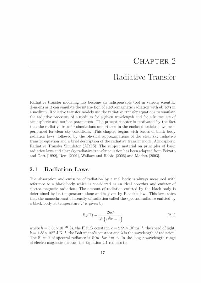
Radiative transfer modeling has become an indispensable tool in various scientificdomains as it can simulate the interaction of electromagnetic radiation with objects ina medium. Radiative transfer models use the radiative transfer equations to simulatethe radiative processes of a medium for a given wavelength and for a known set ofatmospheric and surface parameters. The present chapter is motivated by the factthat the radiative transfer simulations undertaken in the enclosed articles have beenperformed for clear sky conditions. This chapter begins with basics of black bodyradiation laws, followed by the physical approximations of the clear sky radiativetransfer equation and a brief description of the radiative transfer model AtmosphericRadiative Transfer Simulator (ARTS). The subject material on principles of basicradiation laws and clear sky radiative transfer equation has been adapted from Peixotoand Oort [1992], Rees [2001], Wallace and Hobbs [2006] and Modest [2003].
2.1 Radiation Laws
The absorption and emission of radiation by a real body is always measured withreference to a black body which is considered as an ideal absorber and emitter ofelectro-magnetic radiation. The amount of radiation emitted by the black body isdetermined by its temperature alone and is given by Planck’s law. This law statesthat the monochromatic intensity of radiation called the spectral radiance emitted bya black body at temperature T is given by
Bλ(T) =2hc2
λ5(e
hcλkT − 1
) (2.1)
where h = 6.63×10⁻³⁴ Js, the Planck constant, c = 2.99×10⁸ms−1, the speed of light,k = 1.38×10²³ J K−1, the Boltzmann’s constant and λ is the wavelength of radiation.The SI unit of spectral radiance is Wm−2sr−1m−1. In the longer wavelength rangeof electro-magnetic spectra, the Equation 2.1 reduces to
17

18 Radiative Transfer
Figure 2.1: Azimuth angle (ψ), zenith angle(θ) and solid angle as related to a unithemisphere. Source: Modest [2003].
Bλ(T) =2ckT
λ4(2.2)
Equation 2.2 represents the Rayleigh-Jeans expression. The total intensity of theblack body radiation is obtained by integrating the Planck function (Equation 2.1)over the entire wavelength range from 0 to ∞.
B(T ) =
∫ ∞
0
Bλ(T)dλ (2.3)
Integrating Equation 2.3 over all angles of the hemisphere covering a horizonal surfacegives the total flux (W m−2) emitting into all directions from that surface:∫
B(T )cosθdw = σT 4 (2.4)
where σ is the Stefan-Boltzmann constant, θ is the angle between the radiation di-rection and normal to the surface, dw = sinθdθdψ is the solid angle, in sphericalco-ordinate system ψ is called the azimuth angle and θ is called the zenith angle.Figure 2.1 shows the solid angle as related to a unit hemisphere. Equation 2.4 showsthat the flux density emitted by a black body is proportional to the fourth power ofabsolute temperature and this law is called the Stefan-Boltzmann law. Taking thederivative of Equation 2.1 and setting it to zero yields another important law forblack body radiation called the Wien-displacement law, given by
λmaxT = constant (2.5)

2.2. Clear Sky Radiative Transfer Equation 19
According to the Wien-displacement law, as the temperature of the black bodyincreases the peak emission wavelengths shift to the shorter wavelength side of theelectro-magnetic spectrum. This law has been applied to gain an understanding ofthe peak emission wavelength of the Earth. Knowing the surface temperature ofthe Earth which is around 293 K, this law estimates the peak emission wavelengthat 10 μm. Conversely, by the same principle, the surface temperature of the sun iscalculated to be around 6100 K from its known peak emission wavelength (0.5 μm).
A physical body is neither a perfect absorber nor a perfect emitter of electromag-netic radiation as compared to a black body. But the radiation laws derived for theblack body can be extended to study the behavior of non-black body objects. Towardsthis, it is useful to define the emissivity and the absorptivity of a non-black body ma-terial. Emissivity of a non-black body object is defined as the ratio of monochromaticintensity of radiation emitted by the body to the corresponding black body radiation.
ελ =Iλ(emitted)
Bλ(T)(2.6)
The emissivity of a real body depends on many factors such as temperature, itsphysical and chemical composition, its geometrical structure, its surface roughness,its emission wavelength etc. The absorptivity of a real body can be defined as
αλ =Iλ(absorbed)
Iλ(incident)(2.7)
Another law governing radiation is the Kirchhoff’s law which states that for an objectunder thermodynamic equilibrium, the emissivity is equivalent to the absorptivity(ελ = αλ).
2.2 Clear Sky Radiative Transfer Equation
For a clear sky radiative transfer calculation, only absorption and emission of themedium are considered, avoiding the scattering term which usually occurs in thepresence of clouds for infrared and microwave wavelengths. Consider radiation ofintensity Iλ at wavelength λ travelling through an absorbing and emitting atmosphere.The change in its intensity due to absorption after travelling through a small layerof thickness dz is −kλIλρdz, where ρ is the density (mass per unit volume) of themedium, kλ is the mass absorption coefficient (area per unit mass). According toKirchhoff’s law, a selective absorber at any wavelength λ is also a selective emitterof radiation at the same wavelength, therefore the intensity emitted in the directionof propagation is kλBλ(T )ρdz. The net change in the intensity of radiation aftertravelling through a layer dz is given by [Peixoto and Oort, 1992, Rees, 2001],
dIλ = −kλIλρdz + kλBλ(T )ρdz (2.8)
where Bλ(T ) is the black body monochromatic radiance specified by Planck’s law.Equation 2.8 is called Schwarzchild’s equation and is the basic equation for the clear
20 Radiative Transfer
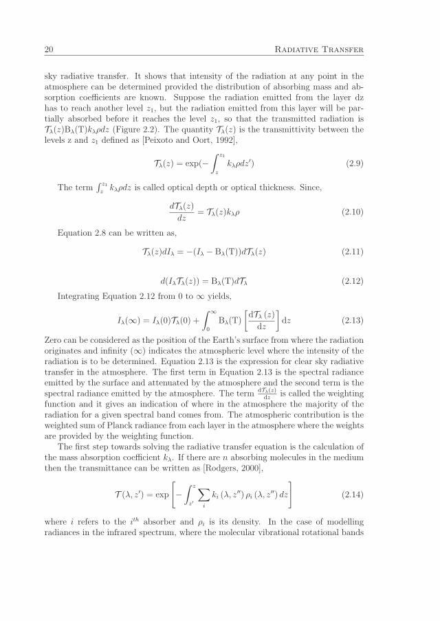
sky radiative transfer. It shows that intensity of the radiation at any point in theatmosphere can be determined provided the distribution of absorbing mass and ab-sorption coefficients are known. Suppose the radiation emitted from the layer dzhas to reach another level z1, but the radiation emitted from this layer will be par-tially absorbed before it reaches the level z1, so that the transmitted radiation isTλ(z)Bλ(T)kλρdz (Figure 2.2). The quantity Tλ(z) is the transmittivity between thelevels z and z1 defined as [Peixoto and Oort, 1992],
Tλ(z) = exp(−∫ z1
z
kλρdz′) (2.9)
The term∫ z1zkλρdz is called optical depth or optical thickness. Since,
dTλ(z)
dz= Tλ(z)kλρ (2.10)
Equation 2.8 can be written as,
Tλ(z)dIλ = −(Iλ − Bλ(T))dTλ(z) (2.11)
d(IλTλ(z)) = Bλ(T)dTλ (2.12)
Integrating Equation 2.12 from 0 to ∞ yields,
Iλ(∞) = Iλ(0)Tλ(0) +
∫ ∞
0
Bλ(T)
[dTλ (z)
dz
]dz (2.13)
Zero can be considered as the position of the Earth’s surface from where the radiationoriginates and infinity (∞) indicates the atmospheric level where the intensity of theradiation is to be determined. Equation 2.13 is the expression for clear sky radiativetransfer in the atmosphere. The first term in Equation 2.13 is the spectral radianceemitted by the surface and attenuated by the atmosphere and the second term is thespectral radiance emitted by the atmosphere. The term dTλ(z)
dzis called the weighting
function and it gives an indication of where in the atmosphere the majority of theradiation for a given spectral band comes from. The atmospheric contribution is theweighted sum of Planck radiance from each layer in the atmosphere where the weightsare provided by the weighting function.
The first step towards solving the radiative transfer equation is the calculation ofthe mass absorption coefficient kλ. If there are n absorbing molecules in the mediumthen the transmittance can be written as [Rodgers, 2000],
T (λ, z′) = exp
[−∫ z
z′
∑i
ki (λ, z′′) ρi (λ, z
′′) dz
](2.14)
where i refers to the ith absorber and ρi is its density. In the case of modellingradiances in the infrared spectrum, where the molecular vibrational rotational bands

2.3. ARTS 21
are important, the absorption coefficients should be summed over large number ofspectral lines.
ki (λ, z′′) =
∑j
kij [T (z′′)] fij [λ, p(z
′′), T (z′′)] (2.15)
where kij is the strength of jth line of the ith absorber and fij is its normalised shape.Any radiative transfer model which models absorption using the above procedure iscalled line by line radiative transfer model.
The line shape f specifies the broadening of absorption lines due to the motion andcollision of gas molecules. There are two kinds of line broadening, Doppler broadeningand pressure broadening. The Doppler broadening is a result of random motion ofgas molecules towards and away from the source of radiation. The shape factor f forthe Doppler broadening is given by
f =1
αD
√πexp
[ν − ν0αD
](2.16)
where ν0 is the wavelength of the line center and αD is the half width of line which isthe distance between the center of the line and the points at which the amplitude isequal to half of the peak amplitude (Figure 2.3). αD is given by
αD =ν0c
(2kT
m
)1/2
(2.17)
where m is the mass of the molecule, k is the Boltzmann’s constant, T is the tem-perature and c is the velocity of light. Pressure broadening is associated with themolecular collision and the shape factor f for the pressure broadening, the so calledLorentz line shape is given by
f =α
π[(ν − ν0)
2 + α2] (2.18)
The line width α in Equation 2.18 is proportional to pressure and is given by
α ∝ p
TN(2.19)
The N ranges from 12to 1 depending on molecular species. Below 20 km altitude in
the atmosphere, the pressure broadening is the contributing factor for line broadeningwhereas above 50 km altitude where the molecular collisions are less frequent, theDoppler broadening is the dominating factor. Between 20 and 50 km altitude, theline shape is the convolution of the Doppler and the Lorentz line shape.
2.3 ARTS
ARTS is a line by line radiative transfer model which can simulate radiances for thespectral region spanning from infrared to microwave [Buehler et al., 2005, Eriksson

22 Radiative Transfer
Figure 2.2: Transmission of radiation through atmosphere.
–5 –4 –3 –2 –1
Doppler
Lorentz
(ν − ν0)/α
1 2 3 4 50
k ν
Figure 2.3: Absorption line shape associated with Doppler broadening and pressurebroadening. Source: Wallace and Hobbs [2006].

2.3. ARTS 23
-0.8 -0.6 -0.4 -0.2 0.0 0.2Jacobian [ K / 1 ]
0
2
4
6
8
10
12
14
Alti
tude
[ km
]
18
-0.8 -0.6 -0.4 -0.2 0.0 0.2Jacobian [ K / 1 ]
0
2
4
6
8
10
12
1419
-0.8 -0.6 -0.4 -0.2 0.0 0.2Jacobian [ K / 1 ]
0
2
4
6
8
10
12
1420
-0.8 -0.6 -0.4 -0.2 0.0 0.2Jacobian [ K / 1 ]
0
2
4
6
8
10
12
14
Alti
tude
[ km
]
18
-0.8 -0.6 -0.4 -0.2 0.0 0.2Jacobian [ K / 1 ]
0
2
4
6
8
10
12
1419
-0.8 -0.6 -0.4 -0.2 0.0 0.2Jacobian [ K / 1 ]
0
2
4
6
8
10
12
1420
Figure 2.4: Water vapour Jacobians for AMSU-B channels 18,19 and 20. The upperand lower panels represent moist tropical atmosphere and dry mid latitude winteratmosphere, respectively. Simulations for nadir and off nadir views of the instrumentare indicated as solid and dotted lines, respectively. Source: John [2005].
et al., 2011]. ARTS solves the radiative transfer equation for ID, 2D or 3D atmo-spheric geometries. The simulations in this thesis have been performed with ARTS forone-dimensional geometry where the atmospheric variables (temperature and gaseousconcentrations) are allowed to vary only in the vertical direction. ARTS contains aninbuilt setup to simulate radiances as detected by radiometers such as HIRS andAMSU onboard NOAA satellites for different viewing angles of the instrument. Formodeling the radiances in the infrared, ARTS employs a line by line calculation forcomputing the absorption coefficient. However, modeling the radiances using thismethod is computationally expensive; therefore, an absorption look-up-table is pro-vided within ARTS to expedite the calculation [Buehler et al., 2011]. Further, formicrowave simulations, PWR98 [Rosenkranz, 1998] a complete water vapour absorp-tion model is provided within the ARTS.
ARTS can also simulate the Jacobians for temperature and trace gas concentra-tions, which is generally defined as the partial derivative of radiance with respectto atmospheric parameters influencing it. The straightforward way to evaluate thisquantity is the use of perturbation method where radiances are simulated for a refer-ence state vector and re-determined successively through small perturbations in eachelement of the state vector. This procedure is time consuming due to which ARTScalculates this analytically [Buehler et al., 2005]. For example, the humidity Jaco-bians simulated by ARTS for three different channels of AMSU-B is shown in Figure2.4.

24 Radiative Transfer
Chapter 3
Radiosonde Corrections
Radiosondes are composed of pressure, temperature and humidity sensors (PTUsensors) and other complementary electronics for measuring wind speed and otherparameters. There are a large number of radiosonde sensors in use and here thedescriptions on the principle of operation and instrument details mainly focus on thehumidity sensors of type Vaisala RS92. Vaisala radiosondes are one of the widelyused radiosondes and RS92 is the latest in this family with an improved humiditymeasurement performance [Kampfer, 2013]. The most common type of humiditysensors in radiosondes belong to the thin film capacitors and Vaisala uses one of thebest known sensing elements called Humicap which is being used on its radiosondessince the 1980s [Kampfer, 2013]. These capacitive thin film moisture sensors respondto water vapour uptake by way of dielectric changes. They have a hydroactive porouspolymer material which acts as a sponge for the water molecules wherein the rate ofadsorption of water molecules on to its surface is proportional to the desorption ofgaseous molecules from it porous surface. These sensors measure the relative humidityand is commonly calibrated in terms of RH. The hydroactive polymer in Humicapsensor could be an A-type polymer as in earlier radiosondes or the latest and superiorH-type polymer which is more stable hydrophilic polymer used in the RS90 and RS92radiosondes. The RH is calculated from the measured capacitance from calibrationcurves standardized by the manufacturer [Miloshevich et al., 2001].
This chapter presents an overview of the various types of corrections applied to theVaisala RS92 radiosonde humidity measurements. Though radiosondes are the vitalsources of information on the atmospheric humidity distribution, their data qualityin the upper troposphere is known to be poor [Elliott and Gaffen, 1991, Moradi et al.,2010, Miloshevich et al., 2009, Soden and Lanzante, 1996]. Their data quality issuesmay arise from several factors. Incorrect calibration of the humidity sensors, errorcaused due to solar heating of the humidity sensors and a slow sensor response at lowtemperatures are some of the most plausible reasons. Several studies have highlightedthese errors and have introduced various correction methods [Vomel et al., 2007,Turner et al., 2003, Miloshevich et al., 2001], but these corrections have been found
25

26 Radiosonde Corrections
to be inadequate for the upper tropospheric humidity measurements [Soden et al.,2004]. Recently Miloshevich et al. [2009] applied several humidity corrections onVaisala RS92 sensors. The efficacy of these corrections has been investigated in thesecond article included in the thesis. This chapter has been written with an aim offurnishing the reader with a general idea of the radiosonde correction methods whichcould not be dealt in detail in the second article included in the thesis.
3.1 Radiosonde Correction Methods
The basis of the correction is the removal of bias in the Vaisala RS92 radiosondehumidity measurements through a comparison with three reference instruments ofknown accuracy. These instruments are cryogenic frost-point hygrometer (CFH)which is intended for correction above 700 hPa, a microwave radiometer for lowertroposphere, and a system of 6 calibrated RH probes for the surface. The biases inRS92 humidity measurements were determined by comparing the RS92 measurementswith simultaneous measurements from these instruments and then these biases wereremoved. The correction is a function of pressure (P) and RH and is given by
RHcorr = G(P,RH)× RH (3.1)
where G(P,RH) is the correction factor.
3.1.1 Mean Calibration Bias Correction
The mean calibration correction removes the bias error in the RS92 humidity measure-ments by comparing these measurements against simultaneous measurements fromthree known reference instruments of known accuracy. It has been seen that theRS92 shows a moist relative bias of 3% under moist conditions and 20% under dryconditions with respect to CFH at an altitude of 700 hPa. In the upper troposphere,the RS92 shows a dry relative bias ranging between 5% for moist conditions and 20%for dry conditions [Miloshevich et al., 2009]. The correction factor in Equation 3.1 isinferred from pressure dependent curves determined for several RH intervals as shownin Figure 3.1. The dashed lines in the Figure represents the polynomial approxima-tion for each curve and are the best approximations of RS92 mean bias relative tothe reference instruments. The polynomial coefficients (F(P, RH)) are given for themid-value of each RH interval. The correction factor in G(P, RH) is determined frompressure dependent curve using the polynomial coefficients as given in Figure 3.2.The coefficients are different for day and nighttime measurements.
The mean calibration error can be determined exclusively from nighttime mea-surements (Figure 3.1(a)) whereas Figure 3.1(b) for daytime measurements representsa combination of the mean calibration error and the error due to solar radiation whichwould be quantified separately. The details as to how they are quantified are explainedin the next section. A more accurate result for the mean calibration correction can
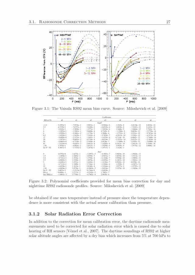
3.1. Radiosonde Correction Methods 27
Figure 3.1: The Vaisala RS92 mean bias curve. Source: Miloshevich et al. [2009]
RH or Fit
Coefficients
a0 a1 a2 a3 a4 a5 a6
Nightb
�1.5 5.1993e+1 �7.9576e�1 3.9051e�3 �8.9666e�6 1.1825e�8 �8.4134e�12 2.4210e�152.5 4.3729e+1 �7.8757e�1 3.8100e�3 �8.4919e�6 1.0830e�8 �7.5247e�12 2.1433e�153 1.0102e+1 �3.5020e�1 1.3771e�3 �1.8918e�6 1.5448e�9 �1.0460e�12 3.7543e�164 �1.2053e+1 �1.3963e�1 5.0608e�4 8.7142e�8 �1.1580e�9 9.6029e�13 �2.2738e�166 �1.9292e+1 �5.3081e�2 1.1776e�5 1.5888e�6 �3.7721e�9 3.2351e�12 �9.7876e�168.5 �1.4220e+1 �1.5629e�1 7.3102e�4 �5.7830e�7 �6.9512e�10 1.1583e�12 �4.3573e�1612 �8.6609e+0 �2.3153e�1 1.1601e�3 �1.6559e�6 4.7114e�10 6.4842e�13 �3.7600e�1620 �1.2075e+1 �9.0493e�2 4.5730e�4 �4.4334e�7 �2.5251e�10 5.6512e�13 �2.1830e�1630 �8.4463e+0 �6.7739e�2 2.1850e�4 2.4128e�7 �1.1680e�9 1.1593e�12 �3.6948e�1642 �7.5226e+0 �9.4287e�2 5.6012e�4 �1.0285e�6 8.1621e�10 �2.4513e�13 3.3189e�18�50 3.7854e+1 �4.9026e�1 2.0313e�3 �3.9299e�6 3.9439e�9 �1.9776e�12 3.8808e�16for P < P2 4.3867e+3 �3.7335e+2 1.2676e+1 �1.9717e�1 1.1628e�3
Dayc
0 6.8793e+0 1.6275e�1 �3.2097e�5 �4.1883e�7 5.0829e�10 �1.9028e�131.9 �1.3058e+1 1.5405e�1 3.0599e�5 �4.9033e�7 5.4030e�10 �1.9315e�132.4 �4.7161e+1 1.3916e�1 1.3784e�4 �6.1264e�7 5.9504e�10 �1.9805e�133.5 �6.0069e+1 1.3320e�1 1.8078e�4 �6.6256e�7 6.1467e�10 �1.9661e�135 �6.6681e+1 1.4741e�1 1.6426e�5 �1.4146e�7 8.9222e�12 4.0390e�1411 �6.7112e+1 1.1009e�1 3.7366e�4 �1.2284e�6 1.2520e�9 �4.3857e�1322 �6.6938e+1 1.1812e�1 2.8349e�4 �1.0166e�6 1.0377e�9 �3.5797e�13�34 �6.0024e+1 1.4726e�1 �6.9462e�5 �2.0216e�7 3.1579e�10 �1.3450e�13for P < P2 5.4021e+3 �3.5312e+2 8.1766e+0 �6.4838e�2SF(a) 9.6886e�1 3.3717e�3 �4.2343e�5 1.7882e�7frac SRE(a) �1.6061e�3 3.7746e�2 �4.7402e�4 2.0018e�6
Figure 3.2: Polynomial coefficients provided for mean bias correction for day andnighttime RS92 radiosonde profiles. Source: Miloshevich et al. [2009]
be obtained if one uses temperature instead of pressure since the temperature depen-dence is more consistent with the actual sensor calibration than pressure.
3.1.2 Solar Radiation Error Correction
In addition to the correction for mean calibration error, the daytime radiosonde mea-surements need to be corrected for solar radiation error which is caused due to solarheating of RH sensors [Vomel et al., 2007]. The daytime soundings of RS92 at highersolar altitude angles are affected by a dry bias which increases from 5% at 700 hPa to

28 Radiosonde Corrections
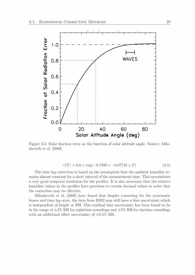
45% in the upper troposphere. The solar radiation error (SRE) is primarily a functionof the incident solar flux which in turn is a function of the solar altitude angle. If thesolar altitude angle is high then SRE in the radiosonde will be higher due to enhancedheating of the RH sensor. Figure 3.1(b) shows the mean calibration bias curve of theRS92 sensor determined during daytime sounding. The polynomial coefficients (F(P,RH, 66 ◦)) for daytime soundings are also given in Figure 3.2 and are provided for ahigher solar altitude angle (66◦). These coefficients represent a combination of meancalibration error and the SRE.
The SRE component of the daytime mean bias is the difference between the day-time and nighttime mean biases (SRE(66◦) =F(P, RH, 66◦)-F(P, RH, night)). TheSRE component in daytime dataset for the other solar altitude angles can be obtainedby multiplying SRE(66◦) with the necessary SRE fraction which can be determinedfrom Figure 3.3 by using the polynomial fit given in Figure 3.2 (frac SRE(α)). Thus,SRE for any solar altitude angle α is given by
SRE(α) = SRE(66◦)× fraction(α) (3.2)
Once the SRE for a particular solar angle is obtained, the coefficients for daytimemeasurements can be obtained by adding the SRE(α) to F (P, RH, night).
F (P,RH, day) = SRE(α) + F (P,RH, night) (3.3)
In brief, the daytime correction for Vaisala RS92 radiosonde consists of correctionfor the mean calibration error (SRE=0) and the correction for SRE.
3.1.3 Time Lag Correction
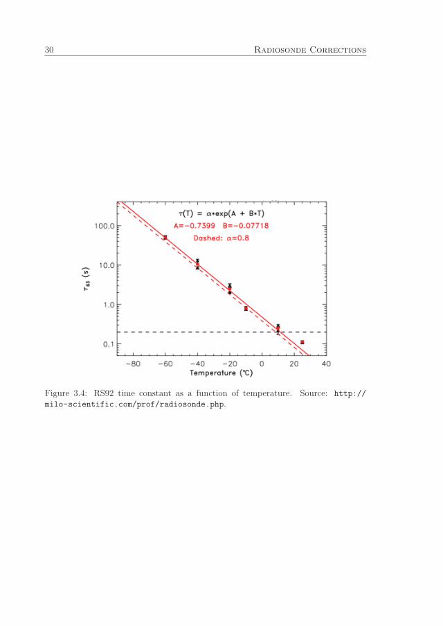
The time lag error is the result of a slow sensor response to changes in the ambienthumidity at low temperatures (−45 ◦C) prevalent in the upper troposphere and thelower stratosphere. The time lag error affects the sensor’s ability to discern thedetailed vertical structure of humidity profile, thus yielding a smooth and incorrectRH profile. The time lag error can be corrected, provided that the sensor timeconstant and the vertical humidity gradient information are known [Miloshevich et al.,2004]. The time constant (τ) refers to the time required for the sensor to respondto 63% of an instantaneous change in the ambient humidity and is a function oftemperature. This value is usually determined in the laboratory. The time constantfor RS92 sensor as a function of temperature is shown in Figure 3.4.
The ambient humidity can be obtained from the measured humidity using theformula
Ua = U+ τ(T )× dU
dt(3.4)
where dUdt
is the local humidity gradient, Ua is the ambient humidity and U is themeasured humidity. The time constant τ is given by
3.1. Radiosonde Correction Methods 29
Figure 3.3: Solar fraction error as the function of solar altitude angle. Source: Milo-shevich et al. [2009]
τ(T ) = 0.8× exp(−0.7399 +−0.07718× T ) (3.5)
The time lag correction is based on the assumption that the ambient humidity re-mains almost constant for a short interval of the measurement time. This necessitatesa very good temporal resolution for the profiles. It is also necessary that the relativehumidity values in the profiles have precision to certain decimal values in order thatthe correction may be effective.
Miloshevich et al. [2009] have found that despite correcting for the systematicbiases and time lag error, the data from RS92 may still have a bias uncertainty whichis independent of height or RH. This residual bias uncertainty has been found to bein the range of ±4% RH for nighttime soundings and ±5% RH for daytime soundingswith an additional offset uncertainty of ±0.5% RH.
30 Radiosonde Corrections
Figure 3.4: RS92 time constant as a function of temperature. Source: http://
milo-scientific.com/prof/radiosonde.php.
Chapter 4
Summary of Papers
This thesis is a compilation of three different scientific articles related to the studyof atmospheric upper tropospheric humidity in observations and models. The firstpaper investigates the importance of radiosonde humidity corrections in the uppertroposphere and how it is important for satellite validation of UTH measurementsin the IR and microwave spectral ranges. The second paper addresses the issue oforbital drift error in polar orbiting satellites and attempts on a method to correct thiserror so as to pave as one of the important steps to create a long term homogenizedtime series to monitor the tropospheric humidity variations. Finally, the third paperdemonstrates the utility of microwave measurements in validating the diurnal cycleof UTH in climate models.
4.1 Paper I
Radiosondes have served as the main sources of atmospheric vertical profile data priorto the deployment of operational weather satellites. These are the primary sourcesof information for validating models and satellite measurements, and their inputs areroutinely used as initial boundary conditions for various numerical weather predictionmodels. However, one major longstanding issue with the radiosonde is the pooraccuracy in determining low water vapour concentrations at higher altitudes such asin the upper troposphere.
This paper mainly demonstrates the importance of radiosonde humidity correc-tions for satellite validation. In this paper various correction methods have beenapplied to the radiosonde humidity measurements which were then compared withsatellite measurements both in the infrared and microwave spectral ranges. This cor-rection has been applied to daytime and nighttime datasets separately. The majorcorrection which is required for the nighttime dataset is the bias removal associatedwith the calibration error in the measurement whereas for the daytime soundings, themajor correction is for the solar radiation error. The application of this correction isshown to be very important for improving the accuracy of radiosonde measurements
31

32 Summary of Papers
of upper troposheric humidity. After application of this correction, the agreementbetween the radiosonde and the satellite measurements for daytime and nighttimecould be improved to a comparable level. This study also cautions against the use ofuncorrected radiosonde measurements for satellite validation.
4.2 Paper II
Climate science today relies on long term climate datasets to monitor climate change.Water vapour, a key climate variable is notably a large player in driving global cli-mate change. At present, long term data records of upper tropospheric humidity areavailable from various polar orbiting satellites which greatly assist in monitoring thevariations of tropospheric humidity. However, it has been observed that over time, theorbital height of these satellites decrease owing to various factors, causing a changein the local sampling time of the satellites and eventually resulting in undesirablealiasing of the diurnal cycle into the time series data obtained from these satellites.
The second paper addresses the issue of orbital drift error on microwave humiditysounder measurements from NOAA and MetOpA satellites, and focuses on correctingthis error in satellite microwave humidity measurements. The study uses data fromthe sensors AMSU-B onboard the NOAA-15, 16 and 17 and MHS onboard the NOAA-18 and MetOpA satellites. As a first step towards correcting the orbital drift error, thediurnal variation of humidity brightness temperatures were constructed by combiningdata from the different polar orbiters and eventually deducing the diurnal samplingbias from them. This paper presents a detailed behavior of the diurnal variabilityof different microwave humidity measurements and their seasonal variations. Theimpact of diurnal correction has been demonstrated on the time-series of NOAA-16channel brightness temperature which detects the surface temperature variations, andUTH channel on NOAA-17 satellites. It is also shown that combining the ascendingand descending time series measurements from NOAA satellites which are affected byorbital drift error cannot completely eliminate the diurnal sampling bias. This studycould be an important link towards the creation of homogenized humidity climatedatasets from microwave measurements of NOAA and MetOpA satellites.
4.3 Paper III
Presently, quantitative answers to our past, present and future climate scenarios arevisualized using global climate models. Many sensitivity studies like as to how theclimate system responds to changes in the various external forcings such as solar in-solation, CO2 concentrations, cloud cover, water vapour concentrations etc., dependson these climate models. However, several sub-scale processes such as convection andcloud are parameterized, therefore the models have to be validated against observa-tions to assess the reliability of the simulations.
In paper 3, we evaluate the UTH diurnal cycle simulation in two different climate

4.3. Paper III 33
models by using microwave satellite measurements as the reference. The diurnalcycle from microwave measurements was generated by combining data from fourdifferent polar orbiting satellites, thus providing 8 samplings at different local timesin a day. These comparisons between models and observations were restricted tosome selected convective land and oceanic regions over the tropics. An IR diurnalcycle has also been constructed from METEOSAT satellite observations for analyzingany differences between the diurnal cycles of IR and microwave. Models exhibitconsiderable differences in the diurnal amplitude and phase relative to the microwaveobservations. Furthermore, a shift in the diurnal phase in IR is observed relative tomicrowave and this can be attributed to the differences in the cloud sensitivity in IRand microwave. It is also demonstrated that a cloud fraction threshold in the rangeof 0.52 to 0.98 is ideal for IR model comparison and the typical values of 0.3–0.4generally used in such comparisons could overcorrect the problem.

34 Summary of Papers

Chapter 5
Conclusions and Future Work
The upper tropospheric humidity and its representation by radiosondes, satellitedata and climate models have been researched in this thesis. Aspects like the diurnalvariation of UTH from satellite measurements and models form an important part ofthe study.
The first article showing the importance of radiosonde corrections is unique inthat it uses satellite measurements to actually depict the importance of these correc-tions. Though there have been various earlier studies which have addressed the issueof errors in radiosonde upper tropospheric humidity measurements and have devel-oped correction procedures to address the same, they have not provided conclusiveevidences of the efficacy of these corrections [Turner et al., 2003, Miloshevich et al.,2001, Soden et al., 2004]. However, our study on the Vaisala RS92 radiosonde correc-tion provides evidence that the correction method can indeed reduce the radiosondedry bias in the upper troposphere. This study also has the potential to serve asa reference when one needs to evaluate the fidelity of future radiosonde humiditycorrections.
An attempt to correct for the orbital drift error in microwave measurements hasbeen presented in the second article. This work is one of the important steps towardsmaking a climate quality long term humidity dataset from microwave measurementsof polar orbiting satellites. A preliminary analysis shown in this work reveals that themethod can address the orbital drift error. The significance of this work is greaterwhen this work is used in conjunction with the other important works on inter-satellitebias correction [John et al., 2012, in press, 2013]. This study is first of its kind inapplying the orbital drift error correction on microwave measurements. The effort tomaking a climate quality dataset from the microwave humidity sounder measurementsis an ongoing work and this paper is one of the results from such a study. As a followup study of this work, the impact of different satellite calibration methods on thediurnal sampling bias correction can be taken up. This impact can be quantified byinferring the trend in the tropospheric humidity measurements.
The evaluation of climate models in simulating the diurnal cycle of UTH using
35

36 Conclusions and Future Work
microwave UTH diurnal cycle measurements has been undertaken in the third article.The differences in IR and microwave diurnal cycles have also been demonstrated inthe study. This is an initial study which uses microwave diurnal cycle to evaluatethe model diurnal cycle and in the long run the plan is to extend this to evaluatethe diurnal cycles of UTH in different climate models participating in the AMIP andCoupled Model Intercomparison Project Phase 5 (CMIP5) projects.

References
R. P. Allan. The Role of Water Vapour in Earth’s Energy Flows. Surveys in Geo-physics, 33:557–564, July 2012. doi: 10.1007/s10712-011-9157-8.
R. P. Allan, M. A. Ringer, and A. Slingo. Evaluation of moisture in the HadleyCentre climate model using simulations of HIRS water-vapour channel radiances.Quarterly Journal of the Royal Meteorological Society, 129:3371–3389, Oct. 2003.doi: 10.1256/qj.02.217.
S. Bony, R. Colman, V. M. Kattsov, R. P. Allan, C. S. Bretherton, J.-L. Dufresne,A. Hall, S. Hallegatte, M. M. Holland, W. Ingram, D. A. Randall, B. J. So-den, G. Tselioudis, and M. J. Webb. How Well Do We Understand and Evalu-ate Climate Change Feedback Processes? J. Climate, 19:3445–3482, 2006. doi:10.1175/JCLI3819.1.
H. Brogniez, R. Roca, and L. Picon. Evaluation of the distribution of subtropicalfree tropospheric humidity in AMIP-2 simulations using METEOSAT water vaporchannel data. Geophys. Res. Lett., 32, 2005. doi: 10.1029/2005GL024341.
S. A. Buehler and V. O. John. A simple method to relate microwave radiances toupper tropospheric humidity. J. Geophys. Res., 110:D02110, 2005. doi: 10.1029/2004JD005111.
S. A. Buehler, P. Eriksson, T. Kuhn, A. von Engeln, and C. Verdes. ARTS, theatmospheric radiative transfer simulator. J. Quant. Spectrosc. Radiat. Transfer, 91(1):65–93, Feb. 2005. doi: 10.1016/j.jqsrt.2004.05.051.
S. A. Buehler, M. Kuvatov, T. R. Sreerekha, V. O. John, B. Rydberg, P. Eriks-son, and J. Notholt. A cloud filtering method for microwave upper tropo-spheric humidity measurements. Atmos. Chem. Phys., 7(21):5531–5542, 2007. doi:10.5194/acp-7-5531-2007.
S. A. Buehler, M. Kuvatov, V. O. John, M. Milz, B. J. Soden, D. L. Jackson, andJ. Notholt. An upper tropospheric humidity data set from operational satellitemicrowave data. J. Geophys. Res., 113:D14110, 2008. doi: 10.1029/2007JD009314.
37

38 References
S. A. Buehler, V. O. John, A. Kottayil, M. Milz, and P. Eriksson. Efficient radiativetransfer simulations for a broadband infrared radiometer — combining a weightedmean of representative frequencies approach with frequency selection by simulatedannealing. J. Quant. Spectrosc. Radiat. Transfer, 111(4):602–615, Mar. 2010. doi:10.1016/j.jqsrt.2009.10.018.
S. A. Buehler, P. Eriksson, and O. Lemke. Absorption lookup tables in the radiativetransfer model ARTS. J. Quant. Spectrosc. Radiat. Transfer, 112(10):1559–1567,2011. doi: 10.1016/j.jqsrt.2011.03.008.
E. Chung, B. J. Soden, B. Sohn, and J. Schmetz. Model-simulated humidity bias inthe upper troposphere and its relation to the large-scale circulation. J. Geophys.Res., 116:D10110, 2011. doi: 10.1029/2011JD015609.
R. Colman. A comparison of climate feedbacks in general circulation models. ClimateDynamics, 20:865–873, 2003. doi: 10.1007/s00382-003-0310-z.
W. P. Elliott and D. J. Gaffen. On the utility of radiosonde humidity archives forclimate studies. Bull. Amer. Met. Soc., 72(10):1507–1520, 1991.
P. Eriksson, S. A. Buehler, C. P. Davis, C. Emde, and O. Lemke. ARTS, the at-mospheric radiative transfer simulator, version 2. J. Quant. Spectrosc. Radiat.Transfer, 112(10):1551–1558, 2011. doi: 10.1016/j.jqsrt.2011.03.001.
D. J. Gaffen, W. P. Elliot, and A. Robock. Relationships between tropospheric watervapor and surface temperature observed radiosonds. Geophys. Res. Lett., 19, 1992.
A. Gettelman, W. D. Collins, E. J. Fetzer, A. Eldering, F. W. Irion, P. B. Duffy, andG. Bala. Climatology of upper-tropospheric relative humidity from the atmosphericinfrared sounder and implications for climate. J. Climate, 19(23):6104–6121, Dec.2006. doi: 10.1175/JCLI3956.1.
H. Goosse, P. Y. Barriat, W. Lefebvre, M. F. Loutre, and V. Zunz, editors. Introduc-tion to climate dynamics and climate modelling. http://www.climate.be/textbook.
A. S. Goudie and D. J. Cuff, editors. Encyclopedia of Global Change, volume 2.Oxford University Press, 2011.
J. Hansen and S. Lebedeff. Global trends of measured surface air temperature. J.Geophys. Res., 92, Nov. 1987. doi: 10.1029/JD092iD11p13345.
I. M. Held and B. J. Soden. Water vapor feedback and global warming. Annu. Rev.Energy Environ., 25:441–475, 2000.
I. M. Held and B. J. Soden. Robust responses of the hydrological cycle to globalwarming. J. Climate, 19(21):5686–5699, 2006. doi: 10.1175/JCLI3990.1.
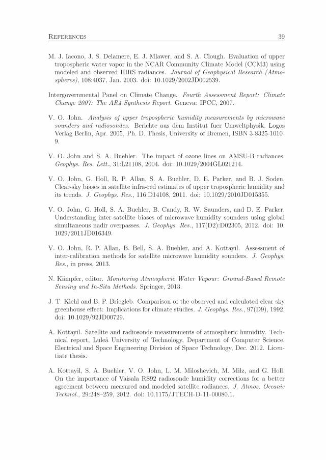
References 39
M. J. Iacono, J. S. Delamere, E. J. Mlawer, and S. A. Clough. Evaluation of uppertropospheric water vapor in the NCAR Community Climate Model (CCM3) usingmodeled and observed HIRS radiances. Journal of Geophysical Research (Atmo-spheres), 108:4037, Jan. 2003. doi: 10.1029/2002JD002539.
Intergovernmental Panel on Climate Change. Fourth Assessment Report: ClimateChange 2007: The AR4 Synthesis Report. Geneva: IPCC, 2007.
V. O. John. Analysis of upper tropospheric humidity measurements by microwavesounders and radiosondes. Berichte aus dem Institut fuer Umweltphysik. LogosVerlag Berlin, Apr. 2005. Ph. D. Thesis, University of Bremen, ISBN 3-8325-1010-9.
V. O. John and S. A. Buehler. The impact of ozone lines on AMSU-B radiances.Geophys. Res. Lett., 31:L21108, 2004. doi: 10.1029/2004GL021214.
V. O. John, G. Holl, R. P. Allan, S. A. Buehler, D. E. Parker, and B. J. Soden.Clear-sky biases in satellite infra-red estimates of upper tropospheric humidity andits trends. J. Geophys. Res., 116:D14108, 2011. doi: 10.1029/2010JD015355.
V. O. John, G. Holl, S. A. Buehler, B. Candy, R. W. Saunders, and D. E. Parker.Understanding inter-satellite biases of microwave humidity sounders using globalsimultaneous nadir overpasses. J. Geophys. Res., 117(D2):D02305, 2012. doi: 10.1029/2011JD016349.
V. O. John, R. P. Allan, B. Bell, S. A. Buehler, and A. Kottayil. Assessment ofinter-calibration methods for satellite microwave humidity sounders. J. Geophys.Res., in press, 2013.
N. Kampfer, editor. Monitoring Atmospheric Water Vapour: Ground-Based RemoteSensing and In-Situ Methods. Springer, 2013.
J. T. Kiehl and B. P. Briegleb. Comparison of the observed and calculated clear skygreenhouse effect: Implications for climate studies. J. Geophys. Res., 97(D9), 1992.doi: 10.1029/92JD00729.
A. Kottayil. Satellite and radiosonde measurements of atmospheric humidity. Tech-nical report, Lulea University of Technology, Department of Computer Science,Electrical and Space Engineering Division of Space Technology, Dec. 2012. Licen-tiate thesis.
A. Kottayil, S. A. Buehler, V. O. John, L. M. Miloshevich, M. Milz, and G. Holl.On the importance of Vaisala RS92 radiosonde humidity corrections for a betteragreement between measured and modeled satellite radiances. J. Atmos. OceanicTechnol., 29:248–259, 2012. doi: 10.1175/JTECH-D-11-00080.1.

40 References
A. Kottayil, V. O. John, and S. A. Buehler. Correcting diurnal cycle aliasing insatellite microwave humidity sounder measurements. J. Geophys. Res., 118(1):101–113, 2013. doi: 10.1029/2012JD018545.
A. Kottayil, S. A. Buehler, and V. O. John. Evaluating the diurnal cycle of uppertropospheric humidity in two different climate models using satellite observations.J. Geophys. Res., under revision 2013.
J. R. Lanzante and G. E. Gahrs. The ”clear-sky bias” of TOVS upper-tropospherichumidity. J. Climate, 13:4034–4041, 2000.
S. Manabe and R. T. Wetherald. Thermal Equilibrium of the Atmosphere with aGiven Distribution of Relative Humidity. Journal of Atmospheric Sciences, 24:241–259, May 1967. doi: 10.1175/1520-0469(1967)024〈0241:TEOTAW〉2.0.CO;2.
L. M. Miloshevich, H. Vomel, A. Paukkunen, A. J. Heymsfield, and S. J. Oltmans.Characterization and correction of relative humidity measurements from vaisalaRS80-A radiosondes at cold temperatures. J. Atmos. Oceanic Technol., 18(2):135–156, 2001. doi: 10.1175/1520-0426(2001)018〈0135:CACORH〉2.0.CO;2.
L. M. Miloshevich, A. Paukkunen, H. Vomel, and S. J. Oltmans. Development andvalidation of a time-lag correction for Vaisala radiosonde humidity measurement.J. Atmos. Oceanic Technol., 21:1305–1327, 2004. doi: 10.1175/1520-0426(2004)021〈1305:DAVOAT〉2.0.CO;2.
L. M. Miloshevich, H. Vomel, D. N. Whiteman, and T. Leblanc. Accuracy assessmentand correction of vaisala RS92 radiosonde water vapor measurements. J. Geophys.Res., 114:D11305, 2009. ISSN 0148-0227. doi: 10.1029/2008JD011565.
M. F. Modest, editor. Radiative Heat Transfer. Academic Press, Newyork, 2003.
I. Moradi, S. A. Buehler, V. O. John, and S. Eliasson. Comparing upper tropospherichumidity data from microwave satellite instruments and tropical radiosondes. J.Geophys. Res., 115:D24310, 2010. doi: 10.1029/2010JD013962.
I. Moradi, H. Meng, R. Ferraro, and S. Bilanow. Correcting geolocation errors formicrowave instruments aboard NOAA satellites. IEEE T. Geosci. Remote, in press2012. doi: 10.1109/TGRS.2012.2220551.
P. P. Peixoto and A. H. Oort, editors. PHYSICS OF CLIMATE. Springer-VerlagNewyork, Inc., 1992.
A. Raval and V. Ramanathan. Observational determination of the greenhouse effect.Nature, 342:758–761, Dec. 1989. doi: 10.1038/342758a0.
A. Raval, A. H. Oort, and V. Ramaswamy. Observed dependence of outgoing longwaveradiation on sea surface temperature and moisture. J. Climate, 7:807–821, 1994.

References 41
W. G. Rees. Physical Principles of Remote Sensing. Cambridge university press, 2edition, 2001. ISBN 978-0-521-66948-1.
C. D. Rodgers, editor. INVERSE METHODS FOR ATMOSPHERIC SOUNDING.World Scientific Publishing Co.Pte.Ltd, 2000.
P. W. Rosenkranz. Water vapor microwave continuum absorption: A comparisonof measurements and models. Radio Sci., 33(4):919–928, 1998. (correction in 34,1025, 1999), ftp://mesa.mit.edu/phil/lbl_rt.
R. J. Ross and D. J. Gaffen. Comment on Widespread tropical atmospher ic dryingfrom 1979 to 1995 by Schroeder and McGuirk. Geophys. Res. Lett., 25:4357–4358,1998. doi: 10.1029/1998GL900169.
E. P. Salathe, Jr. and D. L. Hartmann. A Trajectory Analysis of Tropical Upper-Tropospheric Moisture and Convection. J. Climate, 10:2533–2547, Oct. 1997. doi:10.1175/1520-0442(1997)010〈2533:ATAOTU〉2.0.CO;2.
D. J. Seidel. Water vapor: distribution and trends. In Encyco- pedia of GlobalEnvironmental Change, John Wiley and Sons, Ltd, 2001.
S. C. Sherwood, R. Roca, T. M. Weckwerth, and N. G. Andronova. Troposphericwater vapor, convection, and climate. Rev. Geophys., 48:RG2001, 2010. doi: 10.1029/2009RG000301.
B. J. Soden and F. P. Bretherton. Upper tropospheric relative humidity from theGOES 6.7 μm channel: Method and climatology for july 1987. J. Geophys. Res.,98(D9):16,669–16,688, 1993.
B. J. Soden and I. M. Held. An assessment of climate feedbacks in coupled ocean-atmosphere models. J. Climate, 19(14):3354–3360, 2006.
B. J. Soden and J. R. Lanzante. An assessment of satellite and radiosonde climatolo-gies of upper-tropospheric water vapor. J. Climate, 9:1235–1250, 1996.
B. J. Soden, D. D. Turner, B. M. Lesht, and L. M. Miloshevich. An analysis ofsatellite, radiosonde, and lidar observations of upper tropospheric water vapor fromthe atmospheric radiation measurement program. J. Geophys. Res., 109:D04105,2004. doi: 10.1029/2003JD003828.
B. J. Soden, D. J. Jackson, V. Ramaswamy, M. D. Schwarzkopf, and X. Huang. Theradiative signature of upper tropospheric moistening. Science, 310(5749):841–844,Nov. 2005. doi: 10.1126/science.1115602.
B. J. Soden, I. M. Held, R. Colman, K. M. Shell, J. T. Kiehl, and C. A. Shields.Quantifying Climate Feedbacks Using Radiative Kernels. J. Climate, 21:3504, 2008.doi: 10.1175/2007JCLI2110.1.
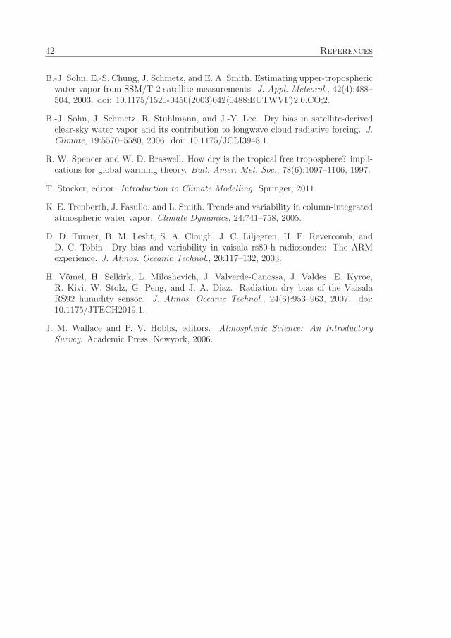
42 References
B.-J. Sohn, E.-S. Chung, J. Schmetz, and E. A. Smith. Estimating upper-troposphericwater vapor from SSM/T-2 satellite measurements. J. Appl. Meteorol., 42(4):488–504, 2003. doi: 10.1175/1520-0450(2003)042〈0488:EUTWVF〉2.0.CO;2.
B.-J. Sohn, J. Schmetz, R. Stuhlmann, and J.-Y. Lee. Dry bias in satellite-derivedclear-sky water vapor and its contribution to longwave cloud radiative forcing. J.Climate, 19:5570–5580, 2006. doi: 10.1175/JCLI3948.1.
R. W. Spencer and W. D. Braswell. How dry is the tropical free troposphere? impli-cations for global warming theory. Bull. Amer. Met. Soc., 78(6):1097–1106, 1997.
T. Stocker, editor. Introduction to Climate Modelling. Springer, 2011.
K. E. Trenberth, J. Fasullo, and L. Smith. Trends and variability in column-integratedatmospheric water vapor. Climate Dynamics, 24:741–758, 2005.
D. D. Turner, B. M. Lesht, S. A. Clough, J. C. Liljegren, H. E. Revercomb, andD. C. Tobin. Dry bias and variability in vaisala rs80-h radiosondes: The ARMexperience. J. Atmos. Oceanic Technol., 20:117–132, 2003.
H. Vomel, H. Selkirk, L. Miloshevich, J. Valverde-Canossa, J. Valdes, E. Kyroe,R. Kivi, W. Stolz, G. Peng, and J. A. Diaz. Radiation dry bias of the VaisalaRS92 humidity sensor. J. Atmos. Oceanic Technol., 24(6):953–963, 2007. doi:10.1175/JTECH2019.1.
J. M. Wallace and P. V. Hobbs, editors. Atmospheric Science: An IntroductorySurvey. Academic Press, Newyork, 2006.

Acronyms
AIRS Atmospheric Infra-Red Sounder. 13
AMIP Atmospheric model inter-comparison project. 13
AMSU Advanced Microwave Sounding Unit. 7
AR4 4th Assessment Report. xiii, 2
ARTS Atmospheric Radiative Transfer Simulator. 17, 21, 23
CAM Community Atmospheric Model. 13
CCM Community Climate Model. 13
CMIP5 Coupled Model Intercomparison Project Phase 5. 35
EBM Energy balance model. 13
EMIC Earth Models of Intermediate Complexity. 13
GCM General Circulation Model. 13
GFDL NOAA Geophysical Fluid Dynamics Laboratory. 13
GHG green house gases. 1, 2
GOES Geostationary Operational Environmental Satellite. 7
HadAM Hadley Centre Climate Model. 13
HIRS High-resolution Infrared Radiation Sounder. 7
IPCC Intergovernmental Panel on Climate Change. xiii, 2
IR infra-red. 7
43
44 Acronyms
MHS Microwave Humidity Sounder. 7
NCAR National Center for Atmospheric Research. 13
NOAA National Oceanic and Atmospheric Administration. 7, 13, 43
OLR Outgoing Longwave Radition. 2, 6
RH Relative Humidity. 1
SSM/T Special Sensor Microwave/Temperature. 7
TOA Top of Atmosphere. 2, 4
UTH Upper Tropospheric Humidity. 2, 6, 7, 13
UTWV Upper Tropospheric Water Vapour. 13

Paper I
On the importance of Vaisala RS92radiosonde humidity corrections for
a better agreement betweenmeasured and modeled satellite
radiances
Authors:A. Kottayil, S. A. Buehler, V. O. John, L. M. Miloshevich, M. Milz, G. Holl
Bibliography:A. Kottayil, S. A. Buehler, V. O. John, L. M. Miloshevich, M. Milz, and G. Holl.On the importance of Vaisala RS92 radiosonde humidity corrections for a betteragreement between measured and modeled satellite radiances. J. Atmos. OceanicTechnol., 29:248–259, 2012. doi: 10.1175/JTECH-D-11-00080.1
45

46
On the Importance of Vaisala RS92 Radiosonde Humidity Corrections for a BetterAgreement between Measured and Modeled Satellite Radiances
AJIL KOTTAYIL AND STEFAN A. BUEHLER
SRT–RY, Lulea University of Technology, Kiruna, Sweden
VIJU O. JOHN
Met Office Hadley Centre, Exeter, United Kingdom
LARRY M. MILOSHEVICH
Milo Scientific LLC, Lafayette, Colorado
M. MILZ AND G. HOLL
SRT–RY, Lulea University of Technology, Kiruna, Sweden
(Manuscript received 5 May 2011, in final form 31 October 2011)
ABSTRACT
A study has been carried out to assess the importance of radiosonde corrections in improving the agreement
between satellite and radiosonde measurements of upper-tropospheric humidity. Infrared [High Resolution
Infrared Radiation Sounder (HIRS)-12] and microwave [Advanced Microwave Sounding Unit (AMSU)-18]
measurements from the NOAA-17 satellite were used for this purpose. The agreement was assessed by
comparing the satellite measurements against simulated measurements using collocated radiosonde profiles
of the Atmospheric Radiation Measurement (ARM) Program undertaken at tropical and midlatitude sites.
The Atmospheric Radiative Transfer Simulator (ARTS) was used to simulate the satellite radiances. The
comparisons have been done under clear-sky conditions, separately for daytime and nighttime soundings.
Only Vaisala RS92 radiosonde sensors were used and an empirical correction (EC) was applied to the ra-
diosonde measurements. The EC includes correction for mean calibration bias and for solar radiation error,
and it removes radiosonde bias relative to three instruments of known accuracy. For the nighttime dataset, the
EC significantly reduces the bias from 0.63 to20.10 K in AMSU-18 and from 1.26 to 0.35 K in HIRS-12. The
EC has an even greater impact on the daytime dataset with a bias reduction from 2.38 to 0.28 K inAMSU-18 and
from 2.51 to 0.59 K in HIRS-12. The present study promises a more accurate approach in future radiosonde-
based studies in the upper troposphere.
1. Introduction
The vertical distribution of water vapor in the tropo-
sphere is quite inhomogeneous, ranging from concen-
trations of a few percent near the surface to only a few
parts per million near the tropopause. Despite the fact
that the upper-tropospheric water vapor constitutes only
a small fraction of the total water vapor, it still has
a large effect on the outgoing longwave radiation (Kiehl
and Briegleb 1992). Model studies suggest that nearly
two-thirds of the total radiative feedback from water
vapor occurs in the upper troposphere (Held and Soden
2000). These studies confirm the need for an accurate
monitoring of the upper-tropospheric humidity (UTH),
which is not verywell simulated in current climatemodels
(John and Soden 2007). One of the sources of UTH
measurements is radiosonde data since themid-twentieth
century. These observations, however, are limited mainly
to land areas and are known to have data quality issues
(Elliott and Gaffen 1991; Miloshevich et al. 2009; Soden
and Lanzante 1996).
Corresponding author address: Ajil Kottayil, Division of Space
Technology, Department of Computer Science, Electrical and
Space Engineering, Lulea University of Technology, Box 812, SE-
98128 Kiruna, Sweden.
E-mail: [email protected]
248 JOURNAL OF ATMOSPHER IC AND OCEAN IC TECHNOLOGY VOLUME 29
DOI: 10.1175/JTECH-D-11-00080.1
� 2012 American Meteorological Society

The satellite era has offered us the advantage of mea-
suring UTH globally, along with a wealth of other in-
formation to understand the earth’s atmospheric system
better. In the microwave and infrared spectral range,
certain frequency ranges are dominated by water vapor
emission from a broad range of pressure levels approxi-
mately between 200 and 500 hPa. These frequency ranges
are suitable for deriving UTH. The typical frequencies
used for this application are 6.7 mm for infrared and 18361 GHz for microwave. The term UTH was first used by
Soden and Bretherton (1993), to describe relative hu-
midity regressed from satellite-observed brightness tem-
peratures obtained by broadband infrared instruments.
A similar approach was followed by Buehler and John
(2005) to derive UTH from microwave measurements
near the 183-GHz water vapor emission line.
Although there have been studies on both infrared
and microwave measurements (Buehler et al. 2004;
Soden and Lanzante 1996), none of the studies thus far
have looked into both instrument types simultaneously
to judge their consistency. For this purpose, the satellite
infrared and microwave measurements have been collo-
cated with radiosonde profiles of the Atmospheric Ra-
diation Measurements (ARM) Program undertaken at
midlatitude and tropical locations. The comparisons were
performed in radiance space by simulating the infrared
and microwave channel radiance from the radiosonde
data using theAtmosphericRadiativeTransfer Simulator
(ARTS; Eriksson et al. 2011).
The relative humidity (RH) measurements from
Vaisala radiosondes are known to have a dry bias in the
upper troposphere (Vomel et al. 2007b; Moradi et al.
2010). Recently, Miloshevich et al. (2009) have im-
plemented an empirical correction procedure to remove
the mean bias error in RS92 radiosonde sensors by
characterizing their accuracy relative to three refer-
ence instruments of known accuracy. We have applied
this correction to the RS92 radiosonde profiles. The
correction is applied for mean calibration bias as a func-
tion of RH and temperature. A correction for solar ra-
diation error resulting from solar heating of the RH
sensor is also applied for daytime soundings. In addition,
a nonbias correction for sensor time lag (TL) error caused
by slow response at low temperature is also examined.
The TL correction recovers vertical structure in the RH
profile that was ‘‘smoothed’’ by slow sensor response
(Miloshevich et al. 2004). Although the time lag cor-
rection is not directly a bias correction, it may remove
some parts of a bias, in particular, in regions with strong
gradients. An important objective of this study is to
assess whether the various corrections improve the
agreement between the radiosonde and satellite data in
both the infrared and microwave bands.
The paper is structured as follows: Section 2 focuses
on the details of measurements and the models and
methods used. Section 3 presents results and discus-
sions on the impact of radiosonde correction procedure
in satellite–radiosonde comparison. Finally, section 4
presents the summary and conclusions.
2. Measurements, models, and methods used
a. Satellite data
The National Oceanic and Atmospheric Administra-
tion (NOAA)-17 satellite carries the Advanced Micro-
wave Sounding Unit (AMSU) and the High Resolution
Infrared Sounder (HIRS)-3. AMSU consists of AMSU-
A andAMSU-B sensors, with a total of 20 channels. The
primary function of the 15-channel AMSU-A (channels
1–15) is to provide temperature sounding of the atmo-
sphere. The five channels of AMSU-B (channels 16–20)
mainly measure water vapor and liquid precipitation
over land and sea. Three channels (18–20) are situated
around the strongwater vapor spectral line at 183.31 GHz
with different offsets from the line center. AMSU-B is a
cross-track, continuous line scanning, total power ra-
diometer with an instantaneous field of view of 1.188 (atthe half-power points), equivalent to a nominal spatial
resolution of 16 km at nadir. The antenna provides
a cross-track scan, scanning649.58 fromnadir with a total
of 90 Earth fields of view per scan line.
HIRS-3 on board NOAA-17 is a 20-channel in-
strument with an instantaneous field of view of 1.388,providing a nominal spatial resolution of 18.9 km at
nadir. The antenna provides a cross-track stepped scan
covering 649.588 from nadir with a total of 56 fields
of view per scan. The spectral characteristics of the
HIRS-3 channels are available online (see http://www.
ncdc.noaa.gov/oa/pod-guide/ncdc/docs/klm/index.htm).
The spectral characteristics differ between different sat-
ellites. Hereafter, the two channels used in inferringUTH
measurements, namely, HIRS channel 12 and AMSU
channel 18, will be referred to as HIRS-12 (6.7 mm) and
AMSU-18 (183 6 1 GHz; Soden and Bretherton 1993;
Buehler and John 2005; Buehler et al. 2008). We have
used measurements of HIRS-12 and AMSU-18 for the
period of 2005–08 on NOAA-17.
b. Radiosonde data and the correction methods
The ARM program operated by the U.S. Department
of Energy launches radiosondes from several dedicated
sites. We have used radiosonde data from 2005 to 2008
of two stations: one in the Southern Great Plains (SGP)
at 36.618N, 97.498W in the United States, and one in
the tropical western Pacific, located at 12.428S, 130.888E
FEBRUARY 2012 KOTTAY I L ET AL . 249

near Darwin, on the northwestern coast of Australia.
We have taken day- and nighttime radiosonde data mea-
sured using Vaisala RS92 sensors. The number of profiles
used for nighttime analysis is 624 out of which 457 belong
to SGP and 167 belong to Darwin. All of the 419 profiles
used for daytime analysis belong to SGP. The profiles used
to study the impact of the time lag correction also belong
to SGP.
The accuracy of radiosonde RH measurements in the
upper troposphere is known to be poor. A number of
studies have shown that RS92 radiosonde sensors ex-
hibit a dry bias in the upper troposphere (Vomel et al.
2007b; Moradi et al. 2010). Miloshevich et al. (2009)
have characterized the accuracy of RS92 RH sensors
relative to three water vapor reference instruments of
known accuracy. The reference instruments are a cryo-
genic frost-point hygrometer (CFH; Vomel et al. 2007a),
which quantifies the accuracy of RS92 above 700 mb;
a microwave radiometer, which mainly senses water va-
por in the lower troposphere; and a systemof six calibrated
RH probes at the surface. The RS92mean calibration bias
was determined by comparing RS92 measurements with
simultaneous measurements from these instruments, and
an empirical correction (EC) procedurewas described that
removes the RS92 mean bias as a function of RH and
pressure P,
RHcorr 5 G(P, RH)3RH, (1)
whereG(P, RH) is the correction factor. The correction
factor is determined from the pressure-dependent curve
fits for several RH intervals (Fig. 9 in Miloshevich et al.
2009), with different curve fits for nighttime and daytime
soundings. The bias error that is corrected for nighttime
soundings is the mean sensor calibration bias. The day-
time soundings are additionally affected by an error
caused by solar heating of the RH sensor. Therefore, in
addition to the mean sensor calibration bias correction,
the daytime soundings also require a correction to re-
move the bias resulting from the so-called solar radia-
tion error (SRE). Hence, the bias and the correction for
daytime soundings would be higher than the nighttime
soundings. In presence of clouds the daytime corrections
could, in fact, overcorrect the radiation bias. However,
this is not a factor in this study because only clear con-
ditions were used. We have applied these corrections on
RS92 radiosonde data and quantified their effect by
comparing the corrected data to satellite measurements.
This study uses a modified version of the published
correction for mean calibration bias that improves the
accuracy for very dry conditions, and extends the upper
limit of validity of the correction to encompass the
tropical upper troposphere/lower stratosphere (UT/LS).
The primary difference is that the correctionwas converted
from a function of pressure to a function of temperature
based on the mean T(P) relationship for the soundings
used to derive the correction. Temperature dependence
is more consistent with the actual sensor calibration and
generalizes the correction to atmospheric profiles sub-
stantially differently from themidlatitude soundings used
to derive the correction. Additional details of the modi-
fied correction for mean calibration bias and associated
IDL code can be found online (http://milo-scientific.com/
prof/radiosonde.php).
The correction procedure described by Miloshevich
et al. (2009) also includes a correction for sensor time-
lag error that causes ‘‘smoothing’’ of the measured RH
profile resulting from a slow sensor response at low
temperatures. To see whether the time-lag correction
has a significant role in reducing the brightness temper-
ature bias, a subset ofRS92 profiles was also corrected for
time-lag error as describedbyMiloshevich et al. (2004).A
subset of soundings is used because olderARMdata (and
most operational RS92 data) have integer RH values,
which result in a less accurate time-lag correction because
much of the detailed information important for a time-lag
correction is lost due to ‘‘rounding off’’ of the data. For
this and other reasons, it is recommended that users of
the Vaisala Digicora III data system output the higher-
resolutionRHdata in so-called Floating-Point Electronic
Data Transfer (FLEDT) files rather than the integer RH
values in standard Electronic Data Transfer (EDT) files.
It should be noted here that in December 2010, Vai-
sala updated their data-processing algorithm to include
time-lag and solar radiation corrections that differ from
those of Miloshevich et al. (2009), but this does not in-
clude the correction for the mean calibration bias used
in this study. This change affects only new Digicora III
data systems or older systems updated with software
version 3.64, and the effect on soundings is described in
Vaisala’s ‘‘RS92 data continuity’’ website.
c. Radiative transfer model
The ARTS is a line-by-line radiative transfer model
that simulates radiances from the infrared to the mi-
crowave spectral range (Buehler et al. 2005; Eriksson
et al. 2011). The model uses precalculated absorption
data to speed up the calculation, as described in Eriksson
et al. (2011).
The code is flexible from the user’s point of view and is
freely available, along with comprehensive documen-
tation (http://www.sat.ltu.se/arts/). The ARTS model
has been validated against other models and satellite
measurements (John and Buehler 2005; Melsheimer
et al. 2005; Saunders et al. 2007). The model has been
used for a wide range of atmospheric studies, including
250 JOURNAL OF ATMOSPHER IC AND OCEAN IC TECHNOLOGY VOLUME 29

applications from the infrared to the microwave wave-
length range (Deuber et al. 2005; Fiorucci et al. 2008;
Eriksson et al. 2003).
Buehler et al. (2010) recently implemented a fast
setup to reduce the computational cost of the broadband
radiance simulations of HIRS channels through the rep-
resentative frequency selection by simulated annealing.
The computational cost has been reduced significantly
while keeping the accuracy of the radiance calculations
the same as the conventional line-by-line calculations.
They have shown that the HIRS channel radiances on
NOAA-14 can be simulated with only 133 frequencies.
For comparison, a full line-by-line calculation would
require 72 717 frequencies. The accuracy of this method
is of the order of 0.03 K. This modified setup has been
used for the present study.
Different continuum models have to be used for the
infrared and the microwave spectral range. The ab-
sorption model setups for the two different spectral
ranges are as follows. In the microwave, we have used
PWR98 (Rosenkranz 1998) for H2O lines and contin-
uum and PWR93 (Rosenkranz 1993) for N2 and O2
lines and their respective continua. Furthermore, line
data of O3 was taken from the High Resolution Trans-
mission (HITRAN) 2004 database (Rothman et al. 2003).
In the infrared, line data were taken from HITRAN 2004
while the continua of H2O, CH4, N2, O2, and CO2 were
taken from MT_CKD_1.0 (Mlawer et al. 2003). A model
intercomparison study betweenARTS and the LBLRTM,
an established reference model for the infrared spectral
range was carried out for HIRS-12 on NOAA-14, -15, -16
and -17 satellites. The model comparison approach is de-
scribed in the appendix. The two RT models were found
to agree within a brightness temperature difference of
0.22 K. ARTS includes various algorithms to simulate
the influence of clouds (Davis et al. 2005; Emde et al.
2004). However, for the present study only clear-sky
simulations were performed.
d. Collocations and cloud detection approach
The collocations between NOAA-17 measurements
and ARM radiosondes are based on spatial and tem-
poral constraints. The spatial constraint is implemented
by a target area of a 50-km radius around the radio-
sonde location, as in Buehler et al. (2004). This approx-
imately takes into account the drift of the radiosonde
as it ascends through the atmosphere. The number of
collocated pixels in a target area varies from 2 to 8 for
HIRS-12 and from 10 to 30 for AMSU-18, respectively.
The time constraint imposed on the collocated dataset
is62 h. This should accommodate the time taken for the
radiosonde to reach the satellite-measuring altitude peak
(300 hPa), which is approximately 25 min. Hence, the
radiosonde time in the collocated dataset is the sum
of the radiosonde launch time and 25 min. Radiances
are simulated from radiosonde profiles using ARTS to
match with the satellite-viewing geometry.
A meaningful comparison between satellite measure-
ments and clear-sky RT model simulations is possible
only if themeasurements are free of cloud contamination.
Therefore, we use the cloud detection tests developed by
McMillin and Dean (1982) to filter out contaminated
HIRS pixels from our analysis. Details of this procedure
are as follows:
Each pixel from satellite measurements is subjected
to the following cloud detection tests. The first two tests
are based on the longwave window channel (11 mm)
brightness temperature and are applicable to all of the
measurements:
(i) A pixel is classified as cloudy if its window channel
brightness temperature is too cold (,210 K).
(ii) A pixel is classified as cloudy, if the longwave
window channel brightness temperature is 4 K
cooler than that of the warmest pixel from the
target area.
(iii) If any one of the followings conditions fail for
nighttime measurements, then the pixel is classified
as cloudy:
24:0 K# TB(18)2 TB(8)# 2:0 K,
24:0K# TB(19)2 TB(18)# 2:0 K.
(iv) During the day a pixel is clear if
jTB(18) 2 TB(8)j, 10 K,
where TB(i) is the brightness temperature for a given
HIRS channel i. If there is more than one clear pixel in
the target area, the average over all the clear pixels are
used; otherwise, it is classified as cloudy. This very
stringent clear scene requirement condition satisfies
25%–100% of the target area for HIRS depending on
the cloud cover. We assume that the AMSU-18 pixels
coincident to the clear HIRS-12 pixels are not cloud
contaminated. This could even result in the removal of
the AMSU-18 pixels, which are unaffected by clouds
because of the much higher sensitivity of HIRS mea-
surements to thin clouds.
e. Relation between UTH and brightnesstemperature
The relationship between UTH and brightness tem-
perature TB is given by
ln(UTH) 5 a 1 b3TB, (2)
FEBRUARY 2012 KOTTAY I L ET AL . 251
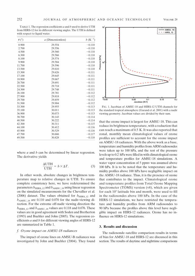
where a and b can be determined by linear regression.
The derivative yields
DUTH
UTH5 b3DT. (3)
In other words, absolute changes in brightness tem-
perature map to relative changes in UTH. To ensure
complete consistency here, we have redetermined the
parameters bHIRS_12 and bAMSU_18 using linear regression
on the simulated measurements for the Chevallier et al.
(2006) dataset. The values obtained for bHIRS_12 and
bAMSU_18 are 0.110 and 0.070 for the nadir-viewing di-
rection. For the extreme off-nadir viewing direction the
bHIRS_12 and bAMSU_18 values are 0.118 and 0.076. These
values are in good agreement with Soden and Bretherton
(1993) and Buehler and John (2005). The regression co-
efficients a and b for different viewing angles of HIRS-12
are summarized in Table 1.
f. Ozone impact on AMSU-18 radiances
The impact of ozone lines on AMSU-B radiances was
investigated by John and Buehler (2004). They found
that the ozone impact is largest for AMSU-18. This can
reduce its brightness temperature, with a reduction that
can reach amaximum of 0.5 K. It was also reported that
zonal, monthly mean climatological values of ozone
profiles are sufficient to account for the ozone impact
onAMSU-18 radiances.With the above work as a base,
temperature and humidity profiles fromARMradiosondes
were taken up to 100 hPa, and the rest of the pressure
levels up to 0.2 hPawere filled inwith climatological ozone
and temperature profiles for AMSU-18 simulations. A
water vapor concentration of 5 ppmv was assumed above
100 hPa. It is to be noted that the temperature and hu-
midity profiles above 100 hPa have negligible impact on
the AMSU-18 radiance. Thus, it is the presence of ozone
that contributes to the impact. Climatological ozone
and temperature profiles from Total Ozone Mapping
Spectrometer (TOMS) version (v8), which are given
for each 108 latitude bin and month, were used to fill
in the radiosondes above 100 hPa. In the case of the
HIRS-12 simulations, we have restricted the tempera-
ture and humidity profiles from ARM radiosondes to
90 hPa because the profiles above this level have negli-
gible impact on HIRS-12 radiances. Ozone has no in-
fluence on HIRS-12 simulations.
3. Results and discussion
The radiosonde–satellite comparison results in terms
of bias for AMSU-18 and HIRS-12 are discussed in this
section. The results of daytime and nighttime comparisons
FIG. 1. Jacobian of AMSU-18 and HIRS-12 UTH channels for
the standard tropical atmosphere (Garand et al. 2001) with a nadir
viewing geometry. Jacobian values are divided by their sum.
TABLE 1. The regression coefficients a and b used to deriveUTH
from HIRS-12 for its different viewing angles. The UTH is defined
with respect to liquid water.
u (8) a (Dimensionless) b (K21)
0.900 29.554 20.110
2.700 29.556 20.110
4.500 29.560 20.110
6.300 29.566 20.110
8.100 29.574 20.110
9.900 29.584 20.110
11.700 29.596 20.110
13.500 29.610 20.110
15.300 29.626 20.111
17.100 29.645 20.111
18.900 29.667 20.111
20.700 29.691 20.111
22.500 29.718 20.111
24.300 29.748 20.111
26.100 29.781 20.112
27.900 29.818 20.112
29.700 29.859 20.112
31.500 29.904 20.112
33.300 29.955 20.113
35.100 30.011 20.113
36.900 30.073 20.113
38.700 30.143 20.114
40.500 30.222 20.114
42.300 30.311 20.115
44.100 30.412 20.116
45.900 30.529 20.116
47.700 30.666 20.117
49.500 30.828 20.118
252 JOURNAL OF ATMOSPHER IC AND OCEAN IC TECHNOLOGY VOLUME 29

are presented separately. The bias is calculated as the
mean of the difference between the simulated and mea-
sured brightness temperature, so a positive bias means
that the radiosondemeasurements are dry and vice versa.
The same convention is followed throughout the dis-
cussion that follows.
The bias value can be used to determine the relative
difference in the UTH measurements between the sat-
ellite and radiosonde. Applying the transformation co-
efficients [bHIRS_12(0.114) and bAMSU_18 (0.073)] in Eq.
(3), it can be inferred that a 1-K bias in AMSU-18 cor-
responds to a relative error of 7% in UTH, whereas for
HIRS-12 it corresponds to a relative difference of 11%.
Even though both AMSU-18 and HIRS-12 measure
UTH, their sensitivity lies at slightly different altitudes.
As shown in Fig. 1, the peak of HIRS-12 sensitivity lies
approximately 2 km higher in altitude than for AMSU-
18. These differences in sensing height will lead to a bias
rather than a random error. Knowing the fact that ra-
diosonde bias is altitude dependent (Miloshevich et al.
2009), the bias for HIRS-12 and AMSU-18 could be
different because the sounding altitudes of the two in-
struments are not the same.
As a separate study to show the impact of ozone in
AMSU-18 simulations,wehave calculated thebiaswith and
without the inclusion of ozone. The nighttime-uncorrected
FIG. 2. Scatterplots of simulated vs observed brightness temperature for AMSU-18 and HIRS-12 (top)
before and (bottom) after empirical correction (correctedRS92) for the nighttime data. Diagonal (black)
and regression (red) lines are shown. The number of data points is 624 for each plot.
TABLE 2. Statistics comparing satellite radiance and simulated
radiance in brightness temperature units for the nighttime dataset.
The bias is defined as the mean of simulated minus measured data.
SD refers to the standard deviation. The number of profiles used is
624. Suffixes bc and ac refers to before and after empirical cor-
rection.
Channel Bias (K)
Bias in
UTH (%) SD (K)
SD UTH
(%)
AMSU-18bc 0.63 24.5 1.66 11.62
AMSU-18ac 20.10 0.7 1.68 11.76
HIRS-12bc 1.26 214.3 1.40 16
HIRS-12ac 0.35 23.9 1.42 16.18
FEBRUARY 2012 KOTTAY I L ET AL . 253

radiosonde datasets were alone chosen for this study.
The results reveal that the inclusion of ozone improved
the bias to 0.63 K from a bias of 0.99 K. Obviously, here
the inclusion of ozone reduces the AMSU-18 brightness
temperature by 0.35 K. This is a clear confirmation that
inclusion of ozone leads to a better agreement between
satellite- and radiosonde-measured UTH as argued by
John and Buehler (2004).
The nighttime comparison results for AMSU-18 and
HIRS-12 are summarized in Table 2. Also, Fig. 2 shows
a scatterplot of simulated versus observed brightness
temperatures for AMSU-18 and HIRS-12 before and
after correction. The empirical correction reduces the
bias from 0.63 to 20.1 K for AMSU-18 and from 1.26
to 0.35 K for HIRS-12. The reduction in the bias is
higher for HIRS-12 (0.91 K) in comparison to AMSU-
18 (0.73 K). The results of daytime analysis are pre-
sented in Table 3. In contrast to the nighttime biases, the
daytime biases in the uncorrected datasets are much
higher (2.38 K in AMSU-18 and 2.51 K in HIRS-12). As
a result, the empirical correction on daytime datasets has
a profound influence in reducing the bias in AMSU-18
and HIRS-12. Accordingly, the bias reduction is of the
order of 2.1 K for AMSU-18 and 1.92 K for HIRS-12.
This clearly is an indication that the corrections are es-
pecially required for all daytime radiosonde observations,
which are subject to solar radiation error. Recall that in
addition to the mean bias correction as applied in the
nighttime dataset, the daytime correction also includes
a correction for solar radiation error, which is most sig-
nificant here.
The bias as a function of brightness temperature bin-
ned at 5-K intervals for the day- and nighttime datasets
is shown in Fig. 3. The reduction in bias resulting from
correction is evident in all brightness temperature ranges,
which represent varying humidity conditions in the upper
FIG. 3. Bias as a function of brightness temperature binned at 5-K intervals before (red) and after (blue)
empirical correction for (left) AMSU-18 and (right) HIRS-12. The standard error (vertical bars), and
(top) nighttime and (bottom) daytime data are shown.
TABLE 3. Statistics comparing satellite radiance and simulated
radiance in brightness temperature units for the daytime dataset.
The bias is defined as the mean of simulated minus measured data.
SD refers to the standard deviation. The number of profiles used is
419. Suffixes bc andac refers to before andafter empirical correction.
Channel Bias (K)
Bias in
UTH (%) SD (K)
SD UTH
(%)
AMSU-18bc 2.38 216.6 1.31 9.17
AMSU-18ac 0.28 21.96 1.39 9.73
HIRS-12bc 2.51 228.61 1.19 13.57
HIRS-12ac 0.59 26.73 1.27 14.48
254 JOURNAL OF ATMOSPHER IC AND OCEAN IC TECHNOLOGY VOLUME 29
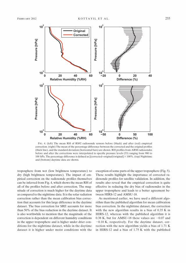
troposphere from wet (low brightness temperature) to
dry (high brightness temperature). The impact of em-
pirical correction on the radiosonde profiles themselves
can be inferred from Fig. 4, which shows the mean RH of
all of the profiles before and after correction. The mag-
nitude of correction is much higher for the daytime data
as compared to the nighttime data. It is the solar radiation
correction rather than the mean calibration bias correc-
tion that accounts for this large difference in the daytime
dataset. The bias correction for SRE accounts for more
than 50% of the bias reduction in the daytime dataset. It
is also worthwhile to mention that the magnitude of the
correction is dependent on different humidity conditions
in the upper troposphere and is higher under drier con-
ditions for the nighttime dataset, while in the daytime
dataset it is higher under moist conditions with the
exception of some parts of the upper troposphere (Fig. 5).
These results highlight the importance of corrected ra-
diosonde profiles for satellite validation. In addition, the
results also reveal that the empirical correction is quite
effective in reducing the dry bias of radiosondes in the
upper troposphere and leads to a better agreement be-
tween HIRS-12 and AMSU-18.
As mentioned earlier, we have used a different algo-
rithm than the published algorithm for mean calibration
bias correction. In the nighttime dataset, the correction
with the new algorithm results in a bias of 0.35 K in
HIRS-12, whereas with the published algorithm it is
0.38 K, but for AMSU-18 these values are 20.07 and
20.10 K, respectively. For the daytime dataset, cor-
rection with the new algorithm yields a bias of 1.71 K
in HIRS-12 and a bias of 1.75 K with the published
FIG. 4. (left) The mean RH of RS92 radiosonde sensors before (black) and after (red) empirical
correction. (right) The mean of the percentage difference between the corrected and the original profiles
(thick line), and the standard deviation (horizontal bars) are shown. RH profiles fromARM radiosondes
before and after the corrections were interpolated to specific pressure levels (53) ranging from 980 to
100 hPa. The percentage difference is defined as [(corrected--original)/original]3 100%. (top) Nighttime
and (bottom) daytime data are shown.
FEBRUARY 2012 KOTTAY I L ET AL . 255

algorithm, while in AMSU-18 these values are 1.76 and
1.78 K, respectively. Although these differences are
small, the use of the new algorithm is recommended for
mean calibration correction because the temperature
dependence is more consistent with actual sensor cali-
bration than the pressure dependence, as used in the
published algorithm.
The impact of the TL correction is shown in Table 4.
This result reveals that the TL correction has a negligible
impact on reducing the bias in AMSU-18 and HIRS-12
because the bias reduction is of the order of only 0.03 K.
Because TL correction needs profiles of higher resolu-
tion, it is applied here only to a subset of RS92 profiles.
A noteworthy observation is that the bias reduction in
AMSU-18 and HIRS-12 resulting from empirical cor-
rection on this subset is the same as that for all of the
RS92 profiles (not shown).
Although the agreement between HIRS-12 and
AMSU-18 has been improved because of correction,
a small discrepancy of the order of 0.45 K for nighttime
and 0.31 K for daytime data still remains. One of the
major reasons for the discrepancy can be attributed to
the uncertainty in the corrected RS92 measurements.
Miloshevich et al. (2009) have shown that the bias un-
certainty is 6(4% 1 0.5% RH), which implies that 4%
of themeasured value plus a 0.5%RHoffset component
is increasingly important for drier conditions. For ex-
ample, the relative uncertainty in the corrected RS92
data is 65% for conditions of 50% RH, 66.5% at 20%
RH,69% at 10%RH, and620%at 3%RH. Therefore,
there could be a larger uncertainty in the correction
occurring at the HIRS-12 sensing altitude than at the
AMSU-18 sensing altitude because it senses a drier at-
mosphere. A part of the difference could also be attrib-
uted to error in the radiative transfermodeling. However,
based on the comparison to LBLRTM described in the
appendix, we expect this error to be smaller than 0.3 K.
Systematic error in the satellite measurements, which
is of the order of 0.5 K in AMSU-18 and HIRS-12 on
NOAA-17, could also play a role (Shi and Bates 2011;
John et al. 2012). It is difficult to attribute the remaining
discrepancy between AMSU-18 and HIRS-12 to any
single cause because it is a very small bias. Therefore,
it is only fair to say that the radiosonde, radiative transfer
modeling, and systematic error in AMSU/HIRS mea-
surements are equally plausible contributors to the bias.
Coming back to the subject of radiosonde correction,
one can state that in addition to significantly reducing
the bias between satellite and radiosonde measurements,
empirical correction also brings forth a better agreement
between AMSU-18 and HIRS-12. The discrepancy in
FIG. 5. The percentage difference between the corrected and original profiles classified in terms of
different humidity conditions in the upper troposphere (dry, moist, andmoderate). Classification is based
on the percentiles of the observed brightness temperature inHIRS-12 such that values$75 percentile are
considered dry,#25 percentile are moist, and values ranging between these as moderate. (left) Nighttime
and (right) daytime data are shown.
TABLE 4. Statistics comparing satellite radiance and simulated
radiance in brightness temperature units for RS92 sensors. The bias
is defined as themean of simulatedminusmeasured data. SD refers
to the standard deviation. The number of profiles used is 85. Suf-
fixes btl and atl refers to before and after time lag correction.
Channel Bias (K)
Bias in
UTH (%) SD (K)
SD UTH
(%)
AMSU-18btl 0.14 20.9 1.52 10.64
AMSU-18atl 0.17 21.2 1.51 10.57
HIRS-12btl 0.94 210.7 1.21 13.80
HIRS-12atl 0.91 210.4 1.19 13.56
256 JOURNAL OF ATMOSPHER IC AND OCEAN IC TECHNOLOGY VOLUME 29

the apparent radiosonde bias between HIRS-12 and
AMSU-18 before correction in the nighttime dataset
was around 10%, and it was lowered to approximately
5% after correction. Similarly, the discrepancy in the
uncorrected daytime dataset was 12%, which reduces
to 4.7% after correction. These results show that the
radiosonde correction is very important in bringing
about a better agreement between satellite and radio-
sonde measurements of UTH.
There have been a number of earlier correction
methods for improving the accuracy of RS80 radiosonde
sensors (Turner et al. 2003; Miloshevich et al. 2001).
However, Soden et al. (2004) showed that these correc-
tion procedures offer only a small improvement in the
upper troposphere, although they are effective in the lower
troposphere. In contrast to this, our work for the RS92
sensors and theMiloshevich et al. (2009) correctionmethod
shows a significant improvement, particularly, in the upper
troposphere. The present study therefore may open up
the possibility of applying a similar correction approach
to other radiosonde sensors.
4. Summary and conclusions
The present study evaluates the importance of radio-
sonde correction in improving the agreement between
satellite- and radiosonde-measured UTH. The satellite
measurements from infrared (HIRS-12) and microwave
(AMSU-18) instruments were used for this purpose. The
satellite measurements were collocated with ARM ra-
diosonde profiles. The satellite–radiosonde comparison
was performed by simulating the radiances from collo-
cated radiosonde profiles using ARTS. The comparisons
were performed only for clear-sky conditions. The em-
pirical correction procedure applied to RS92 radiosonde
sensors was found to have a significant impact in reducing
the bias inAMSU-18 andHIRS-12. The nighttime bias in
AMSU-18 (from 0.63 to 20.10 K) was reduced by 0.73
and by 0.91 K in HIRS-12 (from 1.26 to 0.35 K). During
daytime, the decrease in bias is significantly higher, with
a reduction of 2.1 K (from 2.38 to 0.28 K) in AMSU-18
and 1.92 K (from 2.51 to 0.59 K) in HIRS-12. This is on
account of the bias removal associated with the solar ra-
diation error. The correction also improved the consis-
tency between AMSU-18 and HIRS-12 and reduced the
difference between them by 5% in nighttime and by 7%
in daytime datasets.
In addition to showing the importance of radiosonde
correction for satellite validation, this study also cau-
tions against the use of uncorrected radiosonde profiles
for various water vapor–related studies in the upper
troposphere. The need for such corrections is especially
due to the imperfect characterization and calibration of
the sensor output by the manufacturer. The occurrence
of a similar or worse type of imperfection as addressed
here for Vaisala radiosondes cannot be ruled out for
many other operational radiosondes. In any case, accu-
racy is one aspect that cannot be ignored or compromised
in climate-related studies. The correction method de-
veloped byMiloshevich et al. (2009) and implemented in
this study is an example as to how these errors can be
reduced to a significant extent.
Acknowledgments. The authors are thankful to Lisa
Neclos at NOAA for providing access to NOAA-17
level 1B data. Thanks to the U.S. Department of En-
ergy, Office of Science, Office of Biological and Envi-
ronmental Research,Climate andEnvironmental Sciences
Division for facilitating the use of radiosonde data ob-
tained from their dedicated Atmospheric Radiation
Measurement (ARM) Program. Thanks are also due to
the ARTS radiative transfer community. We acknowl-
edge the LBLRTM community for providing the code.
Special thanks to Eli Mlawer, Oliver Lemke, and Isaac
Moradi. Viju John has been supported by the U.K. Joint
DECC and DEFRAMet Office Hadley Centre Climate
Programme GA01101. This work also contributes to
COST Action ES604–Water Vapour in the Climate
System (WaVaCS). The work of the Kiruna group was
funded by Swedish SpaceBoard, ‘‘SatelliteAtmospheric
Science’’ grant. We thank our three anonymous reviewers
for their useful comments that have resulted in improving
the content and quality of the paper.
APPENDIX
Model Intercomparison
This is a comparison of results from the ARTS and
LBLRTM forward radiance models. LBLRTM (Clough
et al. 2005) has been validated against atmospheric ra-
diance spectra from the ultraviolet to the submillimeter
wavelength range (Turner et al. 2004). In this study in-
frared radiances were simulated using LBLRTMversion
11.6, which uses the modified water vapor continuum
modelMT_CKD_2.4.We verified that continuumchanges
are negligible in the frequency range where HIRS-12 is
located, because ARTS uses MT_CKD_1.0 as the con-
tinuum model. The line parameters are the same as that
for ARTS (HITRAN 2004).
Model intercomparisons were performed for the
HIRSwater vapor channel (HIRS-12) ofNOAA-14, -15,
-16 and -17. The simulations were based on a subset of
the diverse set of atmospheric profiles from the Euro-
pean Centre for Medium-Range Weather Forecasts
FEBRUARY 2012 KOTTAY I L ET AL . 257

(ECMWF) reanalysis data (Chevallier et al. 2006). The
number of used profiles is 4700.
Each channel inHIRS has an individual sensor-response
function (SRF), specifying the weight as a function of
frequency within the spectral range of the channel. The
H2O zenith opacity and the SRF for HIRS-12 is shown
in Fig. A1. In the normal line-by-line calculation mode,
ARTS simulates the radiances within the pass band of
the sensor with a high spectral resolution. These radi-
ances are convolved with the SRF to obtain the radiance
of the HIRS channel. For n-frequency grid points within
the pass band of the jth HIRS channel, the convolved
radiance R( j) is given by
R( j) 5
�n
i51wiri
�n
i51wi
, (A1)
where ri is the radiance for the ith frequency grid point
andwi is the associated weight. The weights for the high-
resolution frequency grids are obtained through in-
terpolation from the sensor-specifiedweights defined for
the frequencies within the SRF. However, the fast setup
for HIRS in ARTS uses only a few frequencies to sim-
ulate the entire HIRS channel radiance. These repre-
sentative frequencies are selected using a simulated
annealing method (Buehler et al. 2010). In the fast setup
for HIRS simulations, the weights for R( j) are derived
using multiple linear regression over a set of line-by-line
calculations using an ensemble of atmospheric conditions.
LBLRTM generates monochromatic infrared radi-
ances with high spectral resolution for a user-specified
frequency range. It has no built-in option to consider the
SRF or other instrumental properties. Thus, to allow
comparison with ARTS, the HIRS channel radiances
have been generated by convolving the high-resolution
spectra with the respective SRF. The Planck function is
used for the conversion of convolved radiance to bright-
ness temperature. During the conversions, care was taken
to ensure that the transformationswere applied to both of
the models in the same manner. Simulations were per-
formed assuming clear-sky conditions and nadir-viewing
geometry with a surface emissivity of 1. The statistics of
comparison for different NOAA satellites sensors are
summarized in Table A1.
REFERENCES
Buehler, S. A., and V. O. John, 2005: A simple method to relate mi-
crowave radiances to upper tropospheric humidity. J. Geophys.
Res., 110, D02110, doi:10.1029/2004JD005111.
——, M. Kuvatov, V. O. John, U. Leiterer, and H. Dier, 2004:
Comparison of microwave satellite humidity data and radio-
sonde profiles: A case study. J. Geophys. Res., 109, D13103,
doi:10.1029/2004JD004605.
——, P. Eriksson, T. Kuhn, A. von Engeln, and C. Verdes, 2005:
ARTS, the atmospheric radiative transfer simulator. J. Quant.
Spectrosc. Radiat. Transfer, 91, 65–93, doi:10.1016/j.jqsrt.2004.05.051.
——,M. Kuvatov, V. O. John, M. Milz, B. J. Soden, D. L. Jackson,
and J. Notholt, 2008: An upper tropospheric humidity data set
from operational satellite microwave data. J. Geophys. Res.,
113, D14110, doi:10.1029/2007JD009314.
——, V. O. John, A. Kottayil, M. Milz, and P. Eriksson, 2010: Ef-
ficient radiative transfer simulations for a broadband infrared
radiometer—Combining a weighted mean of representative
frequencies approach with frequency selection by simulated
annealing. J. Quant. Spectrosc. Radiat. Transf., 111, 602–615,
doi:10.1016/j.jqsrt.2009.10.018.
Chevallier, F., S. Di Michele, and A. P. McNally, 2006: Diverse
profile datasets from the ECMWF 91-level short-range fore-
casts. NWP SAF Satellite Application Facility for Numerical
Weather Prediction Doc. NWPSAF-EC-TR-010, version 1.0,
16 pp. [Available online at http://research.metoffice.gov.uk/
research/interproj/nwpsaf/rtm/profiles_91L.pdf.]
Clough, S. A., and Coauthors, 2005: Atmospheric radiative transfer
modeling: A summary of the AER codes. J. Quant. Spectrosc.
Radiat. Transfer, 91, 233–244, doi:10.1016/j.jqsrt.2004.05.058.
Davis, C., C. Emde, and R. Harwood, 2005: A 3D polarized re-
versed Monte Carlo radiative transfer model for millimeter
and submillimeter passive remote sensing in cloudy atmospheres.
IEEE Trans. Geosci. Remote Sens., 43, 1096–1101, doi:10.1109/
TGRS.2004.837505.
TABLE A1. Statistics comparing ARTS and LBLRTM simula-
tions. The bias is defined as the mean of the difference ARTS
minus LBLRTM. SD refers to the standard deviation.
Satellite Channel Bias (K) SD (K)
NOAA-14 HIRS-12 20.07 0.15
NOAA-15 HIRS-12 20.21 0.23
NOAA-16 HIRS-12 20.17 0.22
NOAA-17 HIRS-12 20.21 0.22
FIG. A1. The H2O zenith opacity spectrum (blue) and the SRF for
HIRS-12 (black) on NOAA-17.
258 JOURNAL OF ATMOSPHER IC AND OCEAN IC TECHNOLOGY VOLUME 29

Deuber, B., J. Morland, L. Martin, and N. Kampfer, 2005: Deriving
the tropospheric integrated water vapor from tipping curve-
derived opacity near 22 GHz. Radio Sci., 40, RS5011,
doi:10.1029/2007RG000233.
Elliott, W. P., and D. J. Gaffen, 1991: On the utility of radiosonde
humidity archives for climate studies. Bull. Amer. Meteor.
Soc., 72, 1507–1520.
Emde, C., S. Buehler, C. Davis, P. Eriksson, T. Sreerekha, and
C. Teichmann, 2004: A polarized discrete ordinate scattering
model for simulations of limb and nadir long-wave measure-
ments in 1-D/3-D spherical atmospheres. J. Geophys. Res.,
109, D24207, doi:10.1029/2004JD005140.
Eriksson, P., C. Jimenez, D. Murtagh, G. Elgered, T. Kuhn, and
S. Buhler, 2003: Measurement of tropospheric/stratospheric
transmission at 10–35 GHz for H2O retrieval in low Earth
orbiting satellite links. Radio Sci., 38, 8069, doi:10.1029/
2002RS002638.
——, S. A. Buehler, C. P. Davis, C. Emde, and O. Lemke, 2011:
ARTS, the atmospheric radiative transfer simulator, version 2.
J. Quant. Spectrosc. Radiat. Transfer, 112, 1551–1558, doi:10.
1016/j.jqsrt.2011.03.001.
Fiorucci, I., and Coauthors, 2008:Measurements of low amounts of
precipitable water vapor by millimeter wave spectroscopy: An
intercomparison with radiosonde, Raman lidar, and Fourier
transform infrared data. J. Geophys. Res., 113, D14314, doi:10.
1029/2008JD009831.
Garand, L., and Coauthors, 2001: Radiance and Jacobian in-
tercomparison of radiative transfer models applied to HIRS
and AMSU channels. J. Geophys. Res., 106 (D20), 24 017–
24 031.
Held, I.M., andB. J. Soden, 2000:Water vapor feedback and global
warming. Annu. Rev. Energy Environ., 25, 441–475.
John, V. O., and S. A. Buehler, 2004: The impact of ozone lines on
AMSU-B radiances.Geophys.Res.Lett., 31,L21108, doi:10.1029/2004GL021214.
——, and ——, 2005: Comparison of microwave satellite humidity
data and radiosonde profiles: A survey of European stations.
Atmos. Chem. Phys., 5, 1843–1853.
——, and B. J. Soden, 2007: Temperature and humidity biases in
global climate models and their impact on climate feedbacks.
Geophys. Res. Lett., 34, L18704, doi:10.1029/2007GL030429.
——, G. Holl, S. A. Buehler, B. Candy, R. W. Saunders, and D. E.
Parker, 2012: Understanding inter-satellite biases of micro-
wave humidity sounders using global SNOs. J. Geophys. Res.,
doi:10.1029/2011JD016349, in press.
Kiehl, J. T., and B. P. Briegleb, 1992: Comparison of the observed
and calculated clear sky greenhouse implications for climate
studies. J. Geophys. Res., 97, 10 037–10 049.
McMillin, L. M., and C. Dean, 1982: Evaluation of a new opera-
tional technique for producing clear radiances. J. Appl.Meteor.,
21, 1005–1014.
Melsheimer, C., and Coauthors, 2005: Intercomparison of general
purpose clear sky atmospheric radiative transfer models for
the millimeter/submillimeter spectral range. Radio Sci., 40,
RS1007, doi:10.1029/2004RS003110.
Miloshevich, L.M., H. Vomel, A. Paukkunen, A. J. Heymsfield, and
S. J. Oltmans, 2001: Characterization and correction of relative
humidity measurements from Vaisala RS80-A radiosondes at
cold temperatures. J. Atmos. Oceanic Technol., 18, 135–156.
——, A. Paukkunen, H. Vomel, and S. J. Oltmans, 2004: De-
velopment and validation of a time-lag correction for Vaisala
radiosonde humidity measurement. J. Atmos. Oceanic Tech-
nol., 21, 1305–1327.——, H. Vomel, D. N. Whiteman, and T. Leblanc, 2009: Accuracy
assessment and correction of Vaisala RS92 radiosonde water
vapor measurements. J. Geophys. Res., 114, D11305, doi:10.
1029/2008JD011565.
Mlawer, E. J., S. A. Clough, and D. C. Tobin, 2003: A new water
vapor continuum model: MT_CKD_1.0. Proc. ARM Sci-
ence Team Meeting, ARM, Broomsfield, CO. [Available
online at http://www.arm.gov/publications/proceedings/conf13/
poster_abs/P00225.]
Moradi, I., S. A. Buehler, V. O. John, and S. Eliasson, 2010:
Comparing upper tropospheric humidity data frommicrowave
satellite instruments and tropical radiosondes. J. Geophys.
Res., 115, D24310, doi:10.1029/2010JD013962.
Rosenkranz, P. W., 1993: Absorption of microwaves by atmo-
spheric gases. Atmospheric Remote Sensing by Microwave
Radiometry,M. A. Janssen, Ed., John Wiley and Sons, 37–90.
——, 1998: Water vapor microwave continuum absorption: A
comparison of measurements and models.Radio Sci., 33, 919–
928; Corrigendum, 34, 1025.Rothman, L. S., and Coauthors, 2003: The HITRAN molecular
spectroscopic database: Edition of 2000 including updates
through 2001. J. Quant. Spectrosc. Radiat. Transfer, 82, 5–44.Saunders, R., and Coauthors, 2007: A comparison of radiative
transfer models for simulating Atmospheric Infrared Sounder
(AIRS) radiances. J. Geophys. Res., 112,D01S90, doi:10.1029/
2006JD007088.
Shi, L., and J. J. Bates, 2011: Three decades of intersatellite-
calibrated High-Resolution Infrared Radiation Sounder up-
per tropospheric water vapor. J. Geophys. Res., 116, D04108,
doi:10.1029/2010JD014847.
Soden, B. J., and F. P. Bretherton, 1993: Upper tropospheric rel-
ative humidity from the GOES 6.7 mm channel: Method and
climatology for July 1987. J. Geophys. Res., 98 (D9), 16 669–
16 688.
——, and J. R. Lanzante, 1996: An assessment of satellite and ra-
diosonde climatologies of upper-tropospheric water vapor.
J. Climate, 9, 1235–1250.——, D. D. Turner, B. M. Lesht, and L. M. Miloshevich, 2004: An
analysis of satellite, radiosonde, and lidar observations of
upper tropospheric water vapor from the Atmospheric Radi-
ation Measurement Program. J. Geophys. Res., 109, D04105,
doi:10.1029/2003JD003828.
Turner, D. D., B. M. Lesht, S. A. Clough, J. C. Liljegren, H. E.
Revercomb, and D. C. Tobin, 2003: Dry bias and variability in
Vaisala RS80-H radiosondes: TheARMexperience. J. Atmos.
Oceanic Technol., 20, 117–132.
——, and Coauthors, 2004: The QMEAERI LBLRTM: A closure
experiment for downwelling high spectral resolution infrared
radiance. J. Atmos. Sci., 61, 2657–2675.
Vomel, H., D. E. David, and K. Smith, 2007a: Accuracy of tropo-
spheric and stratospheric water vapor measurements by the
cryogenic frost point hygrometer: Instrumental details and
observations. J. Geophys. Res., 112, 1–14.
——, andCoauthors, 2007b: Radiation dry bias of theVaisalaRS92
humidity sensor. J. Atmos. Oceanic Technol., 24, 953–963.
FEBRUARY 2012 KOTTAY I L ET AL . 259

Paper II
Correcting diurnal cycle aliasing insatellite microwave humidity
sounder measurements
Authors:A. Kottayil, V. O. John, S. A. Buehler
Bibliography:A. Kottayil, V. O. John, and S. A. Buehler. Correcting diurnal cycle aliasing insatellite microwave humidity sounder measurements. J. Geophys. Res., 118(1):101–113, 2013. doi: 10.1029/2012JD018545
59

60
Correcting diurnal cycle aliasing in satellite microwavehumidity sounder measurements
Ajil Kottayil,1 Viju O. John,2 and Stefan A. Buehler1
Received 24 July 2012; revised 5 December 2012; accepted 5 December 2012; published 16 January 2013.
[1] Microwave humidity measurements from polar orbiting satellites are affected bydiurnal sampling biases which are caused by changes in the local observation time of thesatellites. The long-term data records available from these satellites thus have spurioustrends, which must be corrected. Diurnal cycles of the microwave measurements have beenconstructed by combining data over the period 2001–2010 from five different satelliteplatforms (NOAA-15, -16, -17, -18, and MetOpA). This climatological diurnal cycle hasbeen used to deduce and correct the diurnal sampling bias in Advanced MicrowaveSounding Unit-B and microwave humidity sounder measurements. Diurnal amplitudes forchannels which are sensitive to surface temperature variations show a sharp land-seacontrast with the amplitudes exceeding 10 K for land regions but less than 1 K for oceanicregions. The humidity channels sensitive to the upper and middle troposphere exhibit aseasonal variation with large diurnal amplitudes over convective land regions (often above3 K) in comparison to oceanic regions. The diurnal peak times of these channels overland occur in the early mornings. The diurnal sampling bias correction has a greater impactover land regions when compared to oceanic regions due to the large diurnal amplitudesover land. The diurnal cycle of humidity generated as a part of this study could be usedto evaluate diurnal cycles in climate models.
Citation: Kottayil, A., V. O. John, and S. A. Buehler (2013), Correcting diurnal cycle aliasing in satellite microwave
humidity sounder measurements, J. Geophys. Res. Atmos., 118, 101–113, doi:10.1029/2012JD018545.
1. Introduction
[2] Orbital drift of sun-synchronous satellites can intro-duce artificial trends in climate data records derived fromtheir measurements. For example, Wentz and Schabel[1998] have discussed how the orbital drift of NationalOceanic and Atmospheric Administration (NOAA) satellitesintroduces an artificial cooling trend in the lower tropospherictemperature record derived from Microwave Sounding Unit(MSU) measurements. Orbital parameters of polar orbiting,sun-synchronous satellites are designed to measure the radia-tion emitted from any point on the Earth and its atmosphereat similar local times, thus sampling the same part of the diur-nal cycle of the geophysical parameters measured. However,in reality, factors like atmospheric drag, the deviations fromthe Earth’s spherical shape, the gravitational pull from celestialbodies, and solar activity causes the orbit height to decrease
[e.g., Ignatov et al., 2004], unless it is manually maintainedin a stable orbit (e.g., MetOpA). Such a drift in orbital heightleads to changes in the orbiting period and hence a change inthe local sampling time of the satellites leading to undesirablealiasing of the diurnal cycle into the time series of data fromthe polar orbiters.[3] Different methods have been used to detect and correct
for the orbital drift errors in satellite measurements and theirderived products. For example, orbit drift corrections for theMSU temperature observations have been achieved using thediurnal cycle of simulated observations constructed fromhourly outputs of a general circulation model [Mears et al.,2003]. Jackson and Soden [2007] also corrected for the orbitaldrift error in High-Resolution Infrared Sounder (HIRS) obser-vations using brightness temperatures simulated from the out-put of a climate model. They derived the diurnal sampling biasfrom the simulated brightness temperature time series and thenremoved these biases from the time series of observations.Waliser and Zhou [1997] implemented a rotated empiricalorthogonal function analysis (REOF) to detect the diurnalsampling bias in outgoing long wave radiation (OLR) andhighly reflective cloud (HRC) datasets. They applied REOFto OLR and HRC anomalies and identified those eigenmodeswhich represent the equatorial crossing time changes. Theseeigenmodes were then used to remove the diurnal samplingbias in the OLR and HRC anomaly datasets. Lee et al.[2007] corrected for the diurnal sampling bias in the HIRSOLR data product using the diurnal cycle of OLR which wascreated by aggregating inter-satellite bias corrected monthly
1Division of Space Technology, Department of Computer Science,Electrical and Space Engineering, Luleå University of Technology,Kiruna, Sweden.
2Hadley Center, UK MetOffice, Exeter, UK.
Corresponding author: A. Kottayil, Division of Space Technology,Department of Computer Science, Electrical and Space Engineering, LuleåUniversity of Technology, Kiruna, Sweden. ([email protected])
©2012. American Geophysical Union. All Rights Reserved.2169-897X/13/2012JD018545
101
JOURNAL OF GEOPHYSICAL RESEARCH: ATMOSPHERES, VOL. 118, 101–113, doi:10.1029/2012JD018545, 2013

mean OLR values from different NOAA satellites over a pe-riod of 25 years. Recently, Lindfors et al. [2011] used monthlyclimatology of diurnal cycle of HIRS brightness temperaturesgenerated by combining data for the period 2002–2007 fromdifferent NOAA satellites to derive the diurnal sampling biasin HIRS measurements.[4] In this study, we focus on microwave humidity sounder
measurements from NOAA and MetOpA satellites. Micro-wave data have the advantage of having an almost all-skysampling as compared to only clear-sky sampling for infraredmeasurements [John et al., 2011]. Microwave observationsof humidity from these satellites are available since 1998,and the data have been proven to have a significant impactfor numerical weather prediction [e.g., Andersson et al.,2007]. Indeed, the microwave measurements of atmospherichumidity date back to 1993 with the launch of Special SensorMicrowave/Temperature and Humidity Profile (SSM/T2) asa part of the Defense Meteorological Satellite Program(DMSP). The microwave humidity data measurementsobtained from the NOAA satellites can be composited forsome climate applications [e.g., Xavier et al., 2010], butlong-term homogeneous data are essential for monitoringthe changes in tropospheric water vapor in a warming cli-mate. However, data from the microwave humidity soundersare not homogeneous owing to factors like changes in spec-tral characteristics, sensor degradation, and drift in the satel-lite orbit. In this study, we focus on correcting the orbital drifterror in satellite microwave humidity measurements.[5] This study applies a methodology for the correction of
diurnal sampling biases in microwave humidity measure-ments by first constructing climatological diurnal cycles ofthese measurements by combining data available from fivedifferent platforms for a period of over 10 years. The meth-odology used here is similar to those used in Lee et al.[2007] and Lindfors et al. [2011]. This information is subse-quently used for correcting the orbital drift errors in the hu-midity measurements.[6] The paper is structured as follows: Section 2 gives the
details of satellite data used in the study and the methodsused for combining measurements from different satellites.Section 3 gives details on the construction of diurnal cycleof measurements and error analysis, section 4 provides theresults and discussion, and finally section 5 presents thesummary and conclusions.
2. Satellite Data
[7] The data used in this study are from Advanced Micro-wave Sounding Unit-B (AMSU-B) and microwave humiditysounder (MHS) sensors onboard the NOAA and MetOpAsatellites. AMSU-B is flown on NOAA satellite-15, 16,
and 17, and MHS is on NOAA-18 and MetOpA satellites.They are both five-channel microwave radiometers dedi-cated to measuring atmospheric humidity, an important cli-mate variable [e.g., Held and Soden, 2000], but not verywell simulated by current climate models [e.g., John andSoden, 2007]. Out of the five channels, three (3, 4, and 5)are placed near a strong water absorption line at 183 GHz.The passbands of these channels are 183.31 � 1.00,183.31 � 3.00, and 183.31 � 7.00 GHz (183.31 + 7.00GHz for MHS), respectively. Channels 1 and 2, at 89 and150 GHz (157 GHz for MHS), respectively, look deeperthrough the atmosphere on to the Earth’s surface. Thesechannels are used for the retrieval of ice water path and rainrate [Weng et al., 2003]. Both AMSU-B and MHS sensorsare cross-track scanning instruments with 90 Earth fields-of-view per scan line. Two of the five channels differ be-tween MHS and AMSU-B; the differences are in channels2 and 5, and the characteristics of these biases are describedin [John et al., 2012]. These differences are taken intoaccount during the inter-satellite bias correction procedure.[8] We have used the data spanning the years 2001–2010.
Only channels 1 and 2 of NOAA-15 and NOAA-16 have thefull temporal coverage from 2001 to 2010 as shown in Ta-ble 1. This is due to the high noise in the measurements ofsome of the channels in these satellites after the selected timeperiod. The near-nadir measurements from each satellite foreach day, separately for ascending and descending orbits,were averaged onto 2.5� � 2.5� latitude-longitude grids.Only near-nadir measurements (three measurements on ei-ther side of nadir) are used in this study in order to avoiderrors due to limb effect and scan asymmetry [Buehler et al.,2005; John et al., Monitoring scan asymmetry of microwavehumidity sounding channels using simultaneous all anglecollocations (SAACs), submitted to Journal of GeophysicalResearch, 2012a]. The gridded data contain information onthe number of measurements (N), time of observation (t),and mean and standard deviation (s) of brightness tempera-tures. The data from different satellites gridded in this mannerwas grouped on a monthly basis for 2001–2010. The groupingwas done in such a way that a single grid point can havemultiple data from different satellites for different local times(see Figure 1).[9] A first-order correction of inter-satellite biases are
done for these measurements using data taken during simul-taneous nadir overpasses (SNOs; [Cao et al., 2004]) of thesesatellites. More details on application of SNOs to microwavehumidity measurements are discussed in (John et al., Assess-ment of inter-calibration methods for satellite microwavehumidity sounders, submitted to Journal of GeophysicalResearch, 2012b). All measurements were bias correctedto NOAA-18 measurements, which were taken as referencefor all channels. MetOpA channels have very little bias,within �0.2 K. Channel 1 has the least biases, always within�0.5 K. For NOAA-15, -16, and -17, channel 2 biases areabout 1.5 K due to the shift in frequency from 150 GHzfor AMSU-B to 157 GHz for MHS. Note that these biasesare state dependent and could be up to 3 K in some cases[John et al., 2012]. Channel 3 biases are within �0.5 K.Channel 4 measurements from these satellites have significanttime-varying biases ranging from�1.5 to 2 K. Channel 5 alsohas large biases ranging from �1.5 to 1 K. Note that forNOAA-15 and NOAA-16, channels 3–5 have larger errors
Table 1. The Time Period of the Data Taken from DifferentNOAA and MetOpA Satellites for Constructing the Diurnal Cycleof Different Channels
Channel NOAA-15 NOAA-16 NOAA-17 NOAA-18 MetOpA
1 2001–2010 2001–2010 2003–2010 2006–2010 2007–20102 2001–2010 2001–2010 2003–2010 2006–2010 2007–20103 2001–2006 2001–2006 2003–2010 2006–2010 2007–20104 2001–2006 2001–2006 2003–2010 2006–2010 2007–20105 2001–2006 2001–2006 2003–2010 2006–2010 2007–2010
KOTTAYIL ET AL.: ORBITAL DRIFT CORRECTION
102

than described here after 2006 [John et al., 2012]. Thus,we have not used data of those channels after 2006 in thisstudy. An error analysis is done to account for the uncer-tainties in the estimated inter-satellite biases which are dis-cussed in section 3.
3. Construction of Diurnal Cycle
[10] As can be seen from Figure 1, NOAA 16 has driftedby approximately 5 h over a period of 10 years. This driftcan cause false trends in the time series [Jacobowitz et al.,2003]. On the other hand, this drift has the advantage of facil-itating a better sampling of the diurnal behavior of the mea-surements as shown in Figure 2 and also can lead to shortperiods of global collocations [Holl et al., 2010] which areutilized to understand the radiance dependence of inter-satellite biases [John et al., 2012]. The figure shows measure-ments from all satellites (colored circles) for a grid box overthe Sahara desert for all the Januaries in the study period.Each colored circle in the figure represents daily measure-ment average onto a 2.5� latitude-longitude grid point. Usingthese measurements aggregated for every month over severalyears, a diurnal cycle has been fitted (black curve) for eachgrid point using a second order Fourier series. The Fourier
representation is written as follows [Lee et al., 2007; Lindforset al., 2011]:
Tb tð Þ ¼ a0 þ a1cosp t � t1ð Þ
12þ a2cos
2p t � t2ð Þ
12(1)
where Tb(t) is the brightness temperature, t is the observa-tional local time in hours, a0 is the mean value of Tb, a1 isthe amplitude of the 24 h oscillation, a2 is the amplitude ofthe 12 h oscillation, and t1 and t2 are the phases of the 24and 12 h oscillations, respectively. Expanding equation (1)using simple trignometric identities yields
Tb tð Þ ¼ b0 þ b1cospt12
� �þ b2sin
pt12
� �þ
b3cos2pt12
� �þ b4sin
2pt12
� � (2)
where b0 = a0, b1 ¼ a1cos pt112ð Þ , b2 ¼ a1sin pt1
12ð Þ , b3 ¼a2cos 2pt2
12ð Þ , and b4 ¼ a2sin 2pt212ð Þ . Therefore, the coefficients
a1, a2, t1, and t2 can be determined as
a1 ¼b1
cos pt112ð Þ
(3)
t1 ¼12
ptan�1 b2
b1
� �(4)
Time [ years ]
14
16
18
20
22
Loca
l Tim
e [ h
our
]
NOAA-15
NOAA-16
NOAA-17
NOAA-18
MetOpA
2000 2001 2002 2003 2004 2005 2006 2007 2008 2009 2010 2011
Figure 1. Equator crossing times of the ascending nodes of NOAA and MetOpA satellites which areused in this study.
0 6 12 18 24250
255
260
265
270
275
280
Local Time [hour]
Tb [
K]
Tb [
K]
NOAA15NOAA16NOAA17NOAA18MetOPA
0 6 12 18 24245
250
255
260
265
270
275
280
285
Local Time [hour]
ch2ch3ch4ch5
Figure 2. Left: The diurnal variation in brightness temperature of channel 1 (89 GHz) of a grid point(31.25�N, 1.25�E) over the Sahara desert. The amplitudes a1 and a2 are 5.75 and 2.04 K, respectively.Colored circles represent measurements from different satellites, and the black curve represents the diurnalcycle fit. This is for the month of January. Right: Diurnal fit for channels 2–5 is shown in different colors.
KOTTAYIL ET AL.: ORBITAL DRIFT CORRECTION
103
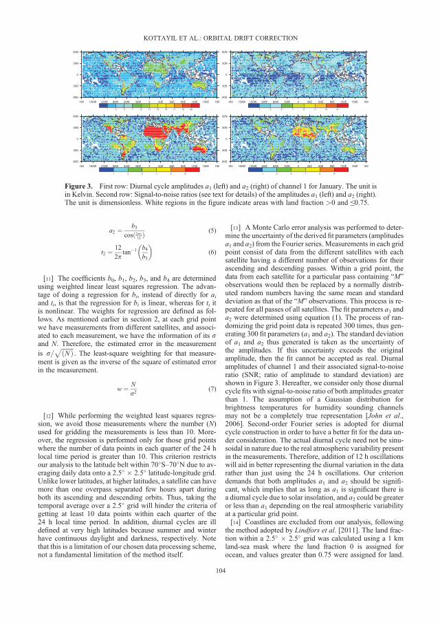
a2 ¼b3
cos 2pt212ð Þ
(5)
t2 ¼12
2ptan�1 b4
b3
� �(6)
[11] The coefficients b0, b1, b2, b3, and b4 are determinedusing weighted linear least squares regression. The advan-tage of doing a regression for bi, instead of directly for aiand ti, is that the regression for bi is linear, whereas for ti itis nonlinear. The weights for regression are defined as fol-lows. As mentioned earlier in section 2, at each grid pointwe have measurements from different satellites, and associ-ated to each measurement, we have the information of its sand N. Therefore, the estimated error in the measurementis s=
ffiffiffiffiffiffiffiffiNð Þ
p. The least-square weighting for that measure-
ment is given as the inverse of the square of estimated errorin the measurement.
w ¼N
s2(7)
[12] While performing the weighted least squares regres-sion, we avoid those measurements where the number (N)used for gridding the measurements is less than 10. More-over, the regression is performed only for those grid pointswhere the number of data points in each quarter of the 24 hlocal time period is greater than 10. This criterion restrictsour analysis to the latitude belt within 70�S–70�N due to av-eraging daily data onto a 2.5� � 2.5� latitude-longitude grid.Unlike lower latitudes, at higher latitudes, a satellite can havemore than one overpass separated few hours apart duringboth its ascending and descending orbits. Thus, taking thetemporal average over a 2.5� grid will hinder the criteria ofgetting at least 10 data points within each quarter of the24 h local time period. In addition, diurnal cycles are illdefined at very high latitudes because summer and winterhave continuous daylight and darkness, respectively. Notethat this is a limitation of our chosen data processing scheme,not a fundamental limitation of the method itself.
[13] A Monte Carlo error analysis was performed to deter-mine the uncertainty of the derived fit parameters (amplitudesa1 and a2) from the Fourier series. Measurements in each gridpoint consist of data from the different satellites with eachsatellite having a different number of observations for theirascending and descending passes. Within a grid point, thedata from each satellite for a particular pass containing “M”observations would then be replaced by a normally distrib-uted random numbers having the same mean and standarddeviation as that of the “M” observations. This process is re-peated for all passes of all satellites. The fit parameters a1 anda2 were determined using equation (1). The process of ran-domizing the grid point data is repeated 300 times, thus gen-erating 300 fit parameters (a1 and a2). The standard deviationof a1 and a2 thus generated is taken as the uncertainty ofthe amplitudes. If this uncertainty exceeds the originalamplitude, then the fit cannot be accepted as real. Diurnalamplitudes of channel 1 and their associated signal-to-noiseratio (SNR; ratio of amplitude to standard deviation) areshown in Figure 3. Hereafter, we consider only those diurnalcycle fits with signal-to-noise ratio of both amplitudes greaterthan 1. The assumption of a Gaussian distribution forbrightness temperatures for humidity sounding channelsmay not be a completely true representation [John et al.,2006]. Second-order Fourier series is adopted for diurnalcycle construction in order to have a better fit for the data un-der consideration. The actual diurnal cycle need not be sinu-soidal in nature due to the real atmospheric variability presentin the measurements. Therefore, addition of 12 h oscillationswill aid in better representing the diurnal variation in the datarather than just using the 24 h oscillations. Our criteriondemands that both amplitudes a1 and a2 should be signifi-cant, which implies that as long as a1 is significant there isa diurnal cycle due to solar insolation, and a2 could be greateror less than a1 depending on the real atmospheric variabilityat a particular grid point.[14] Coastlines are excluded from our analysis, following
the method adopted by Lindfors et al. [2011]. The land frac-tion within a 2.5� � 2.5� grid was calculated using a 1 kmland-sea mask where the land fraction 0 is assigned forocean, and values greater than 0.75 were assigned for land.
Figure 3. First row: Diurnal cycle amplitudes a1 (left) and a2 (right) of channel 1 for January. The unit isin Kelvin. Second row: Signal-to-noise ratios (see text for details) of the amplitudes a1 (left) and a2 (right).The unit is dimensionless. White regions in the figure indicate areas with land fraction >0 and ≤0.75.
KOTTAYIL ET AL.: ORBITAL DRIFT CORRECTION
104

The reason for avoiding coastlines is due to the differencesin the surface emissivity between land and oceanic regions.For surface channels, land has comparatively larger surfaceemissivity (~0.95) in relation to ocean (~ 0.7), and thereforeland appears radiometrically brighter than ocean. So com-bining data over land and ocean makes diurnal cycle lookcompletely different from that generated using either of landor oceanic region alone. This affects surface channels 1 and2 more than the humidity channels over the tropics.[15] There are some differences in our approach of con-
structing a diurnal cycle compared to that of Lindfors et al.[2011]. Lindfors et al. [2011] used individual measurementsin a grid box from different satellites for the diurnal cycle,and therefore there is little scope for taking into accountthe outliers in the measurements. In our approach, since weare gridding the measurements over a 2.5� grid for each passof the satellite for each day and doing a weighted leastsquares regression for determining diurnal cycle amplitudes,two things can be achieved. Taking a daily average will sup-press most of the random variability in the measurements,and secondly, weighted least squares regression will takeinto account the outliers which mostly occur due to highscene inhomogeneity. If the scene is inhomogeneous, lessweight is given for that data point during regression. The di-urnal cycle amplitudes and phases determined using simplelinear regression are not different from that determined bythe approach followed by Lindfors et al. [2011]. But intro-duction of a weighted least squares regression changes thediurnal cycle amplitudes as compared to the simple linearregression approach. For example, for the surface channel1, the differences in amplitude a1 between weighted andsimple linear regression over tropical land is 4.7744 �
2.8927 K, while for amplitude a2, this difference is foundto be 1.3461 � 1.1409 K. The amplitude differences in a1and a2 in channel 1 for tropical ocean are found to be0.8178 �1.0720 and 0.2783 � 0.8766 K, respectively. Forchannel 3, the amplitude differences in a1 and a2 for landis 0.3904 � 0.6686 and 0.3698 � 0.6510 K, respectively,and for ocean the respective differences in a1 and a2 are0.3499 � 0.5543 and 0.3392 � 0.6239 K. A part of thesedifferences in amplitudes arise due to the inclusion of all-sky data in the construction of diurnal cycle.[16] The Monte Carlo error estimates for the amplitudes
are also different from that of Lindfors et al. [2011]. Lindforset al. [2011] use the mean and pooled standard deviation ofthe measurements for generating random measurements ateach grid point. They do not take into account the individualmean and standard deviation of the measurements whichvary and are completely different from one another for dif-ferent satellites and for their ascending and descending over-passes. However, we take into account these differenceswhile generating the random measurements. The effect ofchoosing a slightly different approach for random measure-ments than that of Lindfors et al. [2011] is reflected in theamplitude significance criterion. For example, in channel 3,the number of data points with amplitude a1 and a2 in therange of 0–2 K over the tropics and which satisfies anSNR greater than 1 with our approach is 12% and 20% lessthan that of Lindfors et al. [2011] for a1 and a2, respectively.[17] There are inter-annual variations in the diurnal cycle
amplitudes for different microwave measurements. To testwhether there are any significant differences in the diurnal
cycle amplitudes due to inter-annual variations, we havecompared the amplitudes generated from two consecutiveyears (2003 and 2004) of 6.7 mm channel brightness temper-ature data available from METEOSAT-7 for the month ofJuly. The 6.7 mm channel is sensitive to upper tropospherichumidity variations. The average differences in the diurnalcycle amplitude a1 between two consecutive July monthscomputed within 30�S–30�N latitudes separately for landand oceanic region is found to be 0.26 � 0.24 and 0.21 �
0.19 K, respectively. For amplitude a2, these differencesare 0.12 � 0.113 and 0.0971 � 0.0967 K, respectively.These variations can be even larger between a normal yearand an El Niño–Southern Oscillation (ENSO) year over thetropical Pacific Ocean [Chandra et al., 1998]. It is difficultto quantify these differences with our present approach sincewe rely on combining measurements over several years to geta good temporal resolution so as to construct the diurnal cy-cle. Moreover, combining data over a 10 year period to gen-erate the climatology of diurnal cycle will provide an averagebehavior of the diurnal cycle amplitude taking into accountall the natural variability occurring during those periods.[18] We have also studied for any effect of inter-satellite
bias on the diurnal cycle amplitudes. This was done by intro-ducing a 1 K inter-satellite bias in each of the satellites. Thebias was introduced to one satellite at a time, and the result-ing diurnal amplitudes were compared against the originalamplitudes. Such a comparison would show whether an in-ter-satellite bias in a particular satellite with respect to othersatellites would significantly affect the diurnal cycle. Also itwould highlight if any particular satellite has a greater bear-ing on the diurnal cycle construction. The sensitivity studywas made on channel 3 of the different NOAA satellites,viz., NOAA-15, NOAA-16, NOAA-17, NOAA-18, andMetOpA. The results reveal that there is no significant dif-ference in amplitude a1 with the introduction of a bias ineach of the satellites. However, a2 seems to vary consider-ably with a maximum variation of up to 0.5 K, and this istrue for all the satellites of interest. Inter-satellite biasestherefore seem to have a greater impact on a2 but is insignif-icant for a1.
4. Results and Discussion
[19] In this section, we discuss our analysis of diurnalamplitudes of channels 1 to 5. The discussions begin withan overview of differences in the diurnal amplitudes and theirpeak times as observed in channels 1 to 5. This is followed bya presentation of the annual cycle modulation of the ampli-tudes. Finally, a depiction of the impact of diurnal correctionis given by analyzing the time series of channel 1 brightnesstemperature on NOAA-16 and channel 3 brightness temper-ature time series on NOAA-17 satellites.
4.1. Diurnal Amplitudes
[20] Diurnal amplitudes a1 and a2 for the season December,January, February (DJF) for channels 1 to 5 are shown inFigure 4. The season DJF is selected here because the am-plitude pattern is much more coherent than that obtainedusing any of the other months. In the figure, amplitudes areshown for those regions where the amplitudes a1 and a2 havebeen found to be significant from the Monte Carlo erroranalysis (signal-to-noise ratio>1). The first and second rows
KOTTAYIL ET AL.: ORBITAL DRIFT CORRECTION
105

in the figure show the diurnal amplitudes a1 and a2 ofchannels 1 and 2, respectively, which are mostly sensitiveto surface temperature variations. For these channels, theamplitude a1 is greater than a2 over land regions, whereasover ocean, these differences are not so distinct. The am-plitude is larger over land than over ocean, which is con-sistent with those of Lindfors et al. [2011]. The dry landregions, as in the Australian desert and Sahara region, ex-hibit diurnal amplitude, which in a1 exceed 10 K and in a2exceed 5 K. In addition, large amplitudes are also seen overconvective regions such as the regions in South Africa andSouth America. The oceanic regions which lie in the des-cending branches of the Hadley cell circulation, such as
Southeast Atlantic (20�W–20�E; 15�–30�S) and SoutheastPacific (120�W–70�W; 15�–30�S) show a1 and a2 to beover 2 K in channels 1 and 2. It is in these regions thatthe marine stratocumulus cloud is formed due to subsidenceinversion [Wang et al., 2004]. Under the presence of suchclouds with high liquid water content, the brightness tem-peratures of channels 1 and 2 tend to be warmer than underclear-sky conditions due to the low emissivity of oceanicsurface [Sreerekha et al., 2008]. Therefore, the diurnal cycleseen over those regions is dominated by the diurnal cycleof low level clouds.[21] The third, fourth, and fifth rows of Figure 4 show the
diurnal amplitude of the humidity channels 3–5, which are
Figure 4. Diurnal amplitudes a1 and a2 for channels 1–5 for the season December, January, February(DJF). White regions in the figure indicate areas with SNR ≤ 1 of amplitudes a1 or a2. The first to fifthrows represent diurnal amplitudes for channels 1 to 5. The unit is in Kelvin. Note the different color scalesfor the two different amplitudes in channels 1 and 2.
KOTTAYIL ET AL.: ORBITAL DRIFT CORRECTION
106
sensitive to upper, middle, and lower tropospheric humidity,respectively. These channels are sensitive to relative humidity(RH) variations over broad pressure levels within differentparts of the troposphere. For example, channel 3 is sensitiveto RH changes within 200–500 hPa pressure level, whereasthe sensitivity region for channel 4 lies within 300–800 hPa.Buehler and John [2005] have shown that there exists a linearrelationship between channel 3 brightness temperature andthe channel’s Jacobian weighted relative humidity which isroughly in the 200–500 hPa pressure level. A similar relation-ship exists between channels 4 and 5 brightness temperaturesand relative humidity in the middle and lower troposphere,respectively.[22] For channels 3 and 4, the diurnal amplitude is larger
over land than over ocean. Higher values of diurnal amplitudesare seen over some of the regions over South America andSouth Africa, where convection is intense during the australsummer season (DJF). These observations are consistent withother studies which have shown the diurnal variations in theupper and middle tropospheric humidity using infrared mea-surements [Soden, 2000; Tian et al., 2004; Chung et al.,2007]. The diurnal amplitude a1 in channels 3 and 4 exceeds3 K in convective regions over land. The oceanic regions showa diurnal amplitude of the order of 1 K in channels 3 and 4.The larger values of amplitude a1 in channel 4 as comparedto channel 3 over the Himalayan region can be attributedto the differences in their sensitivity altitudes. Channel 4has a peak sensitivity altitude matching the sensitivity alti-tude of the Himalayan summit, which is around 8 km, whilechannel 3 can partially detect the Himalayan surface with apeak sensitivity altitude at 250 hPa. The amplitude a1 getslarger whenever the sounding channels see the surface. Thiscan be corroborated if one looks at the diurnal amplitude a1of channel 5 (row 5, Figure 4), which detects the lower tro-pospheric humidity, and its diurnal amplitude is governed bychanges in the surface temperature. In contrast to channel 1diurnal amplitudes, the differences in amplitudes a1 and a2for channels 3 and 4 are not so distinct over land regions freeof convection. Over most of the oceanic regions, the diurnalamplitudes a2 of channels 3 and 4 are either comparable toor larger than that of a1. From Figure 4, it is evident that thediurnal amplitude variation of humidity in the upper and mid-dle troposphere is comparable both in terms of magnitude andspatial features. The upper tropospheric humidity data avail-able from microwave measurements thus must be correctedfor diurnal sampling bias, and other issues like clear-sky biasand impact of ozone lines need also be taken into accountfor understanding their trend [Buehler et al., 2008; John andBuehler, 2004; Kottayil et al., 2012; John et al., 2011].[23] The diurnal amplitude of channel 5, which is sensitive to
lower tropospheric humidity variations, shows patterns slightlyreminiscent of channels 1 and 2 but with different magnitudes.This is partly because in very dry regions (southwest of NorthAmerica, Sahara, Gobi desert), channel 5 can detect the sur-face. In moister regions, it generally detects lower tropospherichumidity and therefore differs from surface channels.
4.2. Diurnal Peak Time
[24] Diurnal peak time determined for channels 1 to 5 forthe season DJF is shown in Figure 5. Our definitions for thediurnal peak time are different for surface and humidity chan-nels. This is because channels 1 and 2 are surface channels,
and an increase/decrease in the surface temperature wouldhave a similar effect on channel measurements under clear-sky conditions. However, for channels 3–5, the brightnesstemperature measurements are inversely related to relativehumidity variations, i.e., higher humidity corresponds to alower brightness temperature and vice versa. Therefore, forchannels 1 and 2, diurnal peak time refers to the timecorresponding to maximum brightness temperature inferredfrom diurnal fit. For channels 3–5, the peak time correspondsto the minimum brightness temperature inferred from diurnalfit or to the maximum humidity value.[25] Diurnal peak times for channels 1 and 2 over land
regions occur shortly after noon in local time (12.00 P.M.).This result is consistent considering that the maximum landtemperature due to solar heating occurs in the early after-noon. The early morning peak time shown over most ofthe regions over Southeast Atlantic and Southeast Pacificcoincides with the diurnal peak time of the marine stratocu-mulus clouds [Rozendaal et al., 1995; Wood et al., 2002].Most of the land regions show a diurnal peak time in theearly morning for channels 3 and 4, and this result is consis-tent with other studies which have shown an early morningpeak time for upper and middle tropospheric humidity overland regions [Chung et al., 2007]. An early morning peaktime for channel 3 is exhibited by 40% of oceanic regionswithin the tropics (30�N–30�S), while it is 20% for channel4. Diurnal peak time over most of the regions for channel 5occurs in the early morning. This is due to the surface RHvalues reaching their peak before sunrise and falling as thesurface warms. Since this channel is sensitive to RH varia-tions in the lower troposphere, the peak time will coincidewith the peak time of surface RH value. In dry areas, the sur-face is coldest in the early morning, and this is well moni-tored by channel 5.
4.3. Seasonal Modulation of Diurnal Amplitudes
[26] Figure 6 shows the zonal average of the diurnalamplitudes a1 and a2 over the months for channels 1 to 5over land. The first and second rows of the figure show diur-nal amplitudes for channels 1 and 2, respectively. It is clearfrom the figure that for channels 1 and 2, amplitude a1 ismuch larger than a2. A seasonal shift in the diurnal ampli-tude a1 associated with the movement of Intertropical Con-vergence Zone (ITCZ) is seen. In the Southern Hemisphere,the diurnal amplitude a1 is maximum during austral summerseason and reaches a minimum during austral winter. Simi-larly for the Northern Hemisphere, the amplitude a1 reachesits peak value during boreal summer and a minimum in bo-real winter. This seasonal variation is not so apparent for di-urnal amplitude a2. Diurnal amplitude variations with seasonfor channels 3 and 4 are shown in the third and fourth rowsof Figure 6. The spatial amplitude variations are almost sim-ilar for both channels 3 and 4. Here too, a seasonal shift inthe amplitude is visible for a1. Higher a1 values for channels3 and 4 are observed especially in convective regions lyingclose to the 30�S latitude band during the austral summerseason. This holds also but to a lesser extent for the convec-tive regions in northern equatorial latitudes during the borealsummer season. Such a seasonal variation is not very obvi-ous in a2 for channels 3 and 4. The higher values of ampli-tude observed at higher latitudes cannot be considered asthe real diurnal amplitudes of upper and lower tropospheric
KOTTAYIL ET AL.: ORBITAL DRIFT CORRECTION
107

Figure 5. Diurnal peak time for channels 1–5 for the season DJF. The unit is in hours. White regions inthe figure indicate areas with SNR ≤ 1 of amplitudes a1 or a2. For channels 3–5, the diurnal peak time isthe time corresponding to the maximum humidity value.
KOTTAYIL ET AL.: ORBITAL DRIFT CORRECTION
108

humidity due to dry atmospheric conditions prevailing inthose regions. Dry atmospheres shift the sensitivity altitudeof humidity channels to the surface. Unlike the observationsfrom upper and middle tropospheric channels, no inferenceon seasonal variation can be made from channel 5 diurnalamplitudes.[27] The zonal averages of diurnal amplitudes of oceanic
regions are represented in Figure 7. The first and secondrows of the figure show diurnal amplitudes of channels 1and 2, respectively. Over the tropical oceans, the magnitudesof a1 and a2 are comparable for both the channels. The diur-nal cycle amplitude of sea surface temperature is well below
1 K [Kennedy et al., 2007], and observations greater than1 K shown over tropical oceanic regions are due to the pres-ence of low-level clouds as explained earlier in section 4.1.For channels 1 and 2, a seasonal variation in the diurnalamplitudes is seen over the Southern Ocean and to a lesserextent over northern midlatitudes. The diurnal amplitudesgreater than 1 K shown over the Southern Ocean cannot beentirely attributed to diurnal variations of sea surface tem-perature [Kennedy et al., 2007]; rather, changes in the seasurface emissivity could be a possible contributing factor.The third, fourth, and fifth rows in the figure show the diur-nal amplitudes of channels 3, 4, and 5, respectively. Overall,
Figure 6. Zonal average of the diurnal amplitudes a1 and a2 over the months for channels 1 to 5 for land.The first to fifth rows represent diurnal amplitudes of channels 1 to 5. The unit is in Kelvin, and the whiteareas represent data missing regions.
KOTTAYIL ET AL.: ORBITAL DRIFT CORRECTION
109
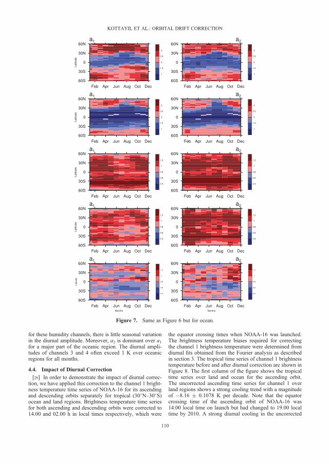
for these humidity channels, there is little seasonal variationin the diurnal amplitude. Moreover, a2 is dominant over a1for a major part of the oceanic region. The diurnal ampli-tudes of channels 3 and 4 often exceed 1 K over oceanicregions for all months.
4.4. Impact of Diurnal Correction
[28] In order to demonstrate the impact of diurnal correc-tion, we have applied this correction to the channel 1 bright-ness temperature time series of NOAA-16 for its ascendingand descending orbits separately for tropical (30�N–30�S)ocean and land regions. Brightness temperature time seriesfor both ascending and descending orbits were corrected to14.00 and 02.00 h in local times respectively, which were
the equator crossing times when NOAA-16 was launched.The brightness temperature biases required for correctingthe channel 1 brightness temperature were determined fromdiurnal fits obtained from the Fourier analysis as describedin section 3. The tropical time series of channel 1 brightnesstemperature before and after diurnal correction are shown inFigure 8. The first column of the figure shows the tropicaltime series over land and ocean for the ascending orbit.The uncorrected ascending time series for channel 1 overland regions shows a strong cooling trend with a magnitudeof �8.16 � 0.1078 K per decade. Note that the equatorcrossing time of the ascending orbit of NOAA-16 was14.00 local time on launch but had changed to 19.00 localtime by 2010. A strong diurnal cooling in the uncorrected
Figure 7. Same as Figure 6 but for ocean.
KOTTAYIL ET AL.: ORBITAL DRIFT CORRECTION
110

time series can be seen since 2006 where a notable drift inNOAA had begun to occur (see Figure 1). After diurnal cor-rection, the trend over tropical land region is found to have amagnitude of only 0.32 � 0.096 K per decade. Over tropicaloceans, the differences in the linear trend shown for uncor-rected and corrected time series is less distinct because thediurnal amplitudes over oceanic regions are small (less than1.5 K). The trend in the uncorrected time series for oceanicregions is 0.6380� 0.0636 K per decade. This positive trendshown over oceanic regions in the uncorrected time series isdue to the behavior of the diurnal cycle over this region. Dueto the presence of low level clouds, the diurnal cycle overoceanic regions peaks in the early morning, and the diurnalwarming in the evening is aliased onto the long-termrecords; this is captured clearly in the uncorrected time seriessince 2006. After diurnal correction, the trend over oceanicregions is only 0.19 � 0.0625 K per decade, which is lessthan a third of the uncorrected trend.[29] The second column of Figure 8 shows the tropical
time series over land and ocean for the descending orbit.Over land, the uncorrected time series shows a cooling trendin the order of�0.26� 0.0831 K per decade, which is due tothe orbital drift causing the equator crossing time of descend-ing orbit to change from 2.00 h in local time at the time oflaunch to 7.00 h in local time by the end of 2010. Subsequentto orbital drift correction, the trend in the tropical time seriesof the ascending orbit is found to be 0.6454 � 0.0768 K perdecade. However over ocean, the trend in the uncorrectedand corrected time series for the descending orbit does notshow significant differences, which are �0.0294 � 0.0632and �0.0637 � 0.0628 K per decade, respectively. The dif-ferences in the trends after diurnal correction shown for bothascending and descending orbits do not come as a surprisesince the correction is for two different local times, at timesof day when the temperatures are at their maximum and min-imum, respectively. Earlier studies as in Vose et al. [2005]have also shown that the trends in the maximum and mini-mum temperatures can be different. Moreover, the trendsare also different for land and ocean due to the differencesin diurnal cycle over these regions as pointed out earlier.[30] We also investigate whether combining ascending
and descending time series could possibly nullify the effectof diurnal cycle aliasing. For this purpose, we combinedthe time series of both ascending and descending orbits of
NOAA-16 channel 1 brightness temperatures before andafter diurnal correction, and the resulting time series fortropical land and ocean are shown in the third column ofFigure 8. The observed trend in channel 1 brightness temper-ature for the combined uncorrected time series over land isfound to be �4.2083 � 0.0811 K per decade, which is onehalf of the trend observed in the uncorrected ascending timeseries. But combining corrected time series results in a trendin the order of 0.4882� 0.0773 K per decade, which is closeto the corrected trend in ascending orbit over land. For trop-ical ocean, the combined uncorrected time series has a trendin the order of 0.3031 �0.0567 K per decade, which is againa half of the trend observed in uncorrected ascending timeseries. Furthermore, combining corrected time series overocean shows a trend of 0.0657 � 0.0560 K per decade,which is within the uncertainty limit of the corrected trendin ascending time series. These results reveal that combiningtime series of ascending and descending orbits which are af-fected by diurnal sampling bias does not completely elimi-nate the spurious trend introduced in the time series. Thisis due to the nonsinusoidal nature of the diurnal cycle ampli-tude arising from a predominance of 12 h oscillations. Onthe other hand, combining time series of ascending and des-cending orbit eliminates to a large extent the 24 h compo-nent of the diurnal cycle. This aspect has been addressed indetail by John et al. (submitted manuscript, 2012b) in thecontext of inter-satellite biases.[31] The impact of diurnal correction on humidity channel
3 is analyzed using the ascending time series of NOAA-17satellite. NOAA-17 is chosen here because of the longevityof the humidity time series in comparison to the other satel-lite data used in this study. Orbital drift is not so significantfor NOAA-17 in comparison to NOAA-16 as the former hasdrifted approximately by only 1 h during the period 2003–2010. The ascending times series of the humidity measure-ments were corrected to 22 h in local time correspondingto the initial equator crossing time of NOAA-17. The uncor-rected and corrected trends in time series observed for chan-nel 3 over tropical land are �0.1621 � 0.1702 and �0.3728� 0.1695 K per decade, respectively, but over ocean thesevalues are �0.6062 � 0.0950 and 0.7259 � 0.0951 K perdecade, respectively. As expected, the trend differences be-tween the corrected and uncorrected time series for channel3 is not so significant due to a lesser orbital drift and smaller
2002 2004 2006 2008 2010275
280
285
290
295
Year
Tb [
K]
Land−Ascending
originalcorrected
2002 2004 2006 2008 2010234
236
238
240
242
Tb [
K]
Tb [
K]
Tb [
K]
Tb [
K]
Tb [
K]
Ocean−Ascending
2002 2004 2006 2008 2010274
276
278
280
282
Year
Land−Descending
2002 2004 2006 2008 2010236
238
240
242Ocean−Descending
2002 2004 2006 2008 2010275
280
285
290
Year
Year Year Year
Land−combine
2002 2004 2006 2008 2010236
238
240
242Ocean−combine
Figure 8. Tropical mean channel 1 brightness temperature times series and linear trends before (redcolor) and after (blue color) diurnal correction for land and ocean. First column is for ascending orbit, sec-ond column is for descending orbit, and third column is for the combined ascending and descendingorbits. A 30 day moving average is applied on time series for clarity.
KOTTAYIL ET AL.: ORBITAL DRIFT CORRECTION
111

diurnal cycle amplitudes. This inference regarding the trendshas been made from a short time series of humidity measure-ments, but a statistically significant trend can be borne outonly when analyzing long time series of humidity measure-ments. A comprehensive analysis is needed to understandthe trends in humidity with a comparatively longer humiditytime series than considered in this study, which would be thefocus of our future studies.
5. Summary and Conclusions
[32] A long-termmonitoring of tropospheric humidity distri-bution over the globe is crucial for predicting the climatechange in the wake of global warming. In this context, long-termmicrowave measurements of tropospheric humidity avail-able fromNOAApolar orbiting satellites play an important rolein identifying the trend in tropospheric humidity. However, themeasurements available from some of these NOAA satellitesare affected by diurnal sampling bias resulting from satelliteorbital drift. In this paper, we have applied a methodologyfor detecting and thereby correcting the diurnal sampling biasin NOAA satellite measurements. A diurnal cycle of satellitemeasurements was generated by combining data correctedfor inter-satellite bias from different NOAA satellites andMetOpA satellite over a period of 10 years using Fourieranalysis. A Monte Carlo error analysis has been performedto assess the significance of the diurnal amplitudes. Diurnalcycles were generated separately for all months for the fivemicrowave channels.[33] An analysis of diurnal cycle amplitudes for surface
channels shows a clear land-sea contrast with the land regionsshowing very high amplitudes often exceeding 10 K over dryand convective regions. These channels also show a seasonalvariation in the diurnal amplitude. The humidity channelssensitive to the upper and middle troposphere also show aseasonal variation in the diurnal amplitude, which can exceed3 K in highly convective land regions and comparativelylower amplitudes over oceanic regions. For these channels,the magnitude of the diurnal amplitudes in 24 and 12 h oscil-lations are not so distinct. Over most of the oceanic regionswithin the tropics, the amplitude of the 12 h oscillation iseither comparable to or greater than that of the 24 h oscillation.The channel sensitive to lower tropospheric humidity doesnot show a seasonal variation in the diurnal amplitude, andthe diurnal amplitude variation in this channel is governedby changes in the surface temperatures and humidity. Thediurnal cycle necessitates adequate sampling requirementsfor new satellite missions, and this should also be taken intoaccount for future model-data comparison [Buehler et al.,2012, 2007; Eliasson, 2011]. The diurnal peak time for upperand middle tropospheric humidity over land regions has anearly morning peak time, which is consistent with previousstudies made using infrared measurements.[34] The impact of diurnal correction has been evaluated
by analyzing the channel 1 brightness temperature time seriesof NOAA-16 and channel 3 brightness temperature time se-ries of NOAA-17 satellites. The results show that for channel1 the diurnal sampling bias correction has a large impact onland regions due to high diurnal cycle amplitudes and a sig-nificantly lower impact on oceanic regions. Also for channel1, combining the ascending and descending time series priorto diurnal sampling correction does not seem to completely
eliminate the spurious trend in time series, which is most likelydue to the predominance of the 12 h oscillations. The analysisof channel 3 brightness temperature time series reveals no sig-nificant difference in the trends in uncorrected and correctedtime series. An exhaustive analysis of humidity time series isbeyond the scope of our present study, but this would be takenup as a follow-up study in our future works. The main motiveof this study was to correct the diurnal cycle aliasing inAMSU-B and MHS satellite measurements. This study isone of the major steps and a prerequisite towards generatinga homogenized humidity dataset for climate studies. However,the diurnal cycle so derived can also be used for the evaluationof the diurnal cycle of humidity in global climate models.
[35] Acknowledgments. We thank our two anonymous reviewers andDavid Parker for their valuable comments. Ajil Kottayil was a visiting scientistat the UK Met Office where a part of this work has been done. V.O.J. wassupported by the UK Joint DECC and DEFRA Integrated ClimateProgramme-GA01101, the UK JWCRP, and EUMETSAT CMSAF. A.K.and S.A.B. were supported by the Swedish Science Council and the SwedishSpace Board. This work contributes to COST Action ES604–Water Vapor inthe Climate System (WaVaCS) and to the EUMETSAT CMSAF activities.Thanks to Lisa Neclos, NOAA CLASS for AMSU-B and MHS Level-1b dataand EUMETSAT NWP-SAF for the AAPP software to process the data.
ReferencesAndersson, E., E. Holm, P. Bauer, A. Beljaars, G. A. Kelly, A. P. McNally,A. J. Simmoons, J.-N. Thpaut, and A. M. Tompkins (2007), Analysis andforecast impact of the main humidity observing systems, Q. J. R.Meteorol. Soc., 133, 1473–1485, doi:10.1002/qj.112.
Buehler, S. A., and V. O. John (2005), A simple method to relate micro-wave radiances to upper tropospheric humidity, J. Geophys. Res., 110,D02110, doi:10.1029/2004JD005111.
Buehler, S. A., M. Kuvatov, and V. O. John (2005), Scan asymmetries inAMSU-B data, Geophys. Res. Lett., 32, L24810, doi:10.1029/2005GL024747.
Buehler, S. A., M. Kuvatov, V. O. John, M.Milz, B. J. Soden, D. L. Jackson,and J. Notholt (2008), An upper tropospheric humidity data set fromoperational satellite microwave data, J. Geophys. Res., 113, D14110,doi:10.1029/2007JD009314.
Buehler, S. A., et al. (2007), A concept for a satellite mission to measure cloudice water path and ice particle size, Q. J. R. Meteorol. Soc., 133(S2),109–128, doi:10.1002/qj.143.
Buehler, S. A., et al. (2012), Observing ice clouds in the submillimeterspectral range: The CloudIce mission proposal for ESA’s Earth Explorer8, Atmos. Meas. Tech., 5, 1529–1549, doi:10.5194/amt-5-1529-2012.
Cao, C., M. Weinreb, and H. Xu (2004), Predicting simultaneous nadir over-passes among polar-orbiting meteorological satellites for the intersatellitecalibration of radiometers, J. Atmos. Oceanic Technol., 21, 537–542.
Chandra, S., J. R. Ziemke, W. Min, and W. G. Read (1998), Effects of1997–1998 El Niño on tropospheric ozone and water vapor, Geophys.Res. Lett., 25, 3867–3870, doi:10.1029/98GL02695.
Chung, E. S., B. J. Sohn, J. Schmetz, and M. Koenig (2007), Diurnalvariation of upper tropospheric humidity and its relations to convectiveactivities over tropical Africa, Atmos. Chem. Phys., 7(10), 2489–2502,doi:10.5194/acp-7-2489-2007.
Eliasson, S. (2011), Ice clouds in satellite observations and climate models,Tech. rep., Luleå University of Technology, Department of ComputerScience, Electrical and Space Engineering Division of Space Technology,licentiate thesis, ISSN: 1402-1757, ISBN: 978-91-7439-312-5.
Held, I. M., and B. J. Soden (2000), Water vapor feedback and globalwarming, Annu. Rev. Energy Environ., 25, 441–475.
Holl, G., S. A. Buehler, B. Rydberg, and C. Jiménez (2010), Collocatingsatellite-based radar and radiometer measurements—Methodology andusage examples, Atmos. Meas. Tech., 3, 693–708, doi:10.5194/amt-3-693-2010.
Ignatov, A., I. Laszlo, E. D. Harrod, K. B. Kidwell, and G. P. Goodrum(2004), Equator crossing times for NOAA, ERS and EOS sun-synchro-nous satellites, Int. J. Remote Sensing, 25(23), 5255–5266, doi:10.1080/01431160410001712981.
Jackson, D. L., and B. J. Soden (2007), Detection and correction of diurnalsampling bias in HIRS/2 brightness temperatures, J. Atmos. OceanicTechnol., 24, 1425–1438, doi:10.1175/JTECH2062.1.
Jacobowitz, H., L. L. Stowe, G. Ohring, A. Heidinger, K. Knapp, and N. R.Nalli (2003), The Advanced Very High Resolution Radiometer Pathfinder
KOTTAYIL ET AL.: ORBITAL DRIFT CORRECTION
112

Atmosphere (PATMOS) Climate Dataset: A resource for climate research.,Bull. Amer. Met. Soc., 84, 785–793, doi:10.1175/BAMS-84-6-785.
John, V. O., and S. A. Buehler (2004), The impact of ozone lines onAMSU-B radiances, Geophys. Res. Lett., 31, L21108, doi:10.1029/2004GL021214.
John, V. O., and B. J. Soden (2007), Temperature and humidity biases inglobal climate models and their impact on climate feedbacks, Geophys.Res. Lett., 34, L18704, doi:10.1029/2007GL030429.
John, V. O., S. A. Buehler, and N. Courcoux (2006), A cautionary note onthe use of Gaussian statistics in satellite based UTH climatologies, IEEEGeosci. R. S. Le., 3(1), 130–134, doi:10.1109/LGRS.2005.859350.
John, V. O., G. Holl, R. P. Allan, S. A. Buehler, D. E. Parker, and B. J.Soden (2011), Clear-sky biases in satellite infra-red estimates of uppertropospheric humidity and its trends, J. Geophys. Res., 116, D14108,doi:10.1029/2010JD015355.
John, V. O., G. Holl, S. A. Buehler, B. Candy, R. W. Saunders, and D. E.Parker (2012), Understanding inter-satellite biases of microwave humid-ity sounders using global simultaneous nadir overpasses, J. Geophys.Res., 117(D2), D02305, doi:10.1029/2011JD016349.
Kennedy, J. J., P. Brohan, and S. F. B. Tett (2007), A global climatology ofthe diurnal variations in sea-surface temperature and implications forMSU temperature trends, Geophys. Res. Lett., 34, L05712, doi:10.1029/2006GL028920.
Kottayil, A., S. A. Buehler, V. O. John, L. M. Miloshevich, M. Milz, andG. Holl (2012), On the importance of Vaisala RS92 radiosonde humiditycorrections for a better agreement between measured and modeled satel-lite radiances, J. Atmos. Oceanic Technol., 29, 248–259, doi:10.1175/JTECH-D-11-00080.1.
Lee, H.-T., A. Gruber, R. G. Ellingson, and I. Laszlo (2007), Development ofthe HIRS outgoing longwave radiation climate dataset, J. Atmos. OceanicTechnol., 24, 2029–2047, doi:10.1175/2007JTECHA989.1.
Lindfors, A. V., I. A. Mackenzie, S. F. B. Tett, and L. Shi (2011), Climato-logical diurnal cycles in clear-sky brightness temperatures from the high-resolution infrared radiation sounder (HIRS), J. Atmos. Oceanic Technol.,28, 1199–1205, doi:10.1175/JTECH-D-11-00093.1.
Mears, C. A., M. C. Schabel, and F. J. Wentz (2003), A reanalysis of theMSU Channel 2 tropospheric temperature record., J. Clim., 16, 3650–3664,doi:10.1175/1520-0442(2003)016< 3650:AROTMC> 2.0.CO;2.
Rozendaal, M. A., C. B. Leovy, and S. A. Klein (1995), An observationalstudy of diurnal variations of marine stratiform cloud., J. Clim., 8,1795–1809, doi:10.1175/1520-0442(1995)008< 1795:AOSODV> 2.0.CO;2.
Soden, B. J. (2000), The diurnal cycle of convection, clouds, and watervapor in the tropical upper troposphere, Geophys. Res. Lett., 27(15),2173–2176.
Sreerekha, T. R., S. A. Buehler, U. O’Keeffe, A. Doherty, C. Emde, andV. O. John (2008), A strong ice cloud event as seen by a microwavesatellite sensor: Simulations and observations, J. Quant. Spectrosc.Radiat. Transfer, 109(9), 1705–1718, doi:10.1016/j.jqsrt.2007.12.023.
Tian, B., B. J. Soden, and X. Wu (2004), Diurnal cycle of convection,clouds, and water vapor in the tropical upper troposphere: Satellites versusa general circulation model, J. Geophys. Res., 109, D10101, doi:10.1029/2003JD004117.
Vose, R. S., D. R. Easterling, and B. Gleason (2005), Maximum and mini-mum temperature trends for the globe: An update through, Geophys. Res.Lett., 2004, 32, L23822, doi:10.1029/2005GL024379.
Waliser, D. E., and W. Zhou (1997), Removing satellite equatorial crossingtime biases from the OLR and HRC datasets., J. Clim., 10, 2125–2146,doi:10.1175/1520-0442(1997)010< 2125:RSECTB> 2.0.CO;2.
Wang, Y., S.-P. Xie, H. Xu, and B. Wang (2004), Regional model simula-tions of marine boundary layer clouds over the Southeast Pacific off SouthAmerica. Part I: Control experiment*,Monthly Weather Review, 132, 274,doi:10.1175/1520-0493(2004)132< 0274:RMSOMB> 2.0.CO;2.
Weng, F., L. Zhao, R. R. Ferraro, G. Poe, X. Li, and N. C. Grody (2003),Advanced microwave sounding unit cloud and precipitation algorithms,Radio Science, 38, 8068, doi:10.1029/2002RS002679.
Wentz, F. J., and M. Schabel (1998), Effects of orbital decay on satellite-derived lower-tropospheric temperature trends, Nature, 394, 661–664,doi:10.1038/29267.
Wood, R., C. S. Bretherton, and D. L. Hartmann (2002), Diurnal cycle ofliquid water path over the subtropical and tropical oceans, Geophys.Res. Lett., 29(23), 2092, doi:10.1029/2002GL015371.
Xavier, P. K., V. O. John, S. A. Buehler, R. S. Ajayamohan, and S. Sijikumar(2010), Variability of Indian summer monsoon in a new upper tropo-spheric humidity data set, Geophys. Res. Lett., 37, L05705, doi:10.1029/2009GL041861.
KOTTAYIL ET AL.: ORBITAL DRIFT CORRECTION
113

74
Paper III
Evaluating the diurnal cycle ofupper tropospheric humidity in two
different climate models usingsatellite observations
Authors:A. Kottayil, S. A. Buehler, V. O. John
Bibliography:A. Kottayil, S. A. Buehler, and V. O. John. Evaluating the diurnal cycle of uppertropospheric humidity in two different climate models using satellite observations. J.Geophys. Res., under revision 2013
75

76

JOURNAL OF GEOPHYSICAL RESEARCH, VOL. ???, XXXX, DOI:10.1029/,
Evaluating the diurnal cycle of upper tropospheric humidity in
two different climate models using satellite observations.
Ajil Kottayil1, Stefan A. Buehler1, Viju O. John2
Abstract. The diurnal cycle of upper tropospheric humidity (UTH) is known to be in-fluenced by such processes as convection and the formation of clouds. These processesneed to be parameterized in global climate models. In this study, we evaluate the per-formance of the climate models CAM-5 and GA-3 in simulating the diurnal cycle of UTHby taking combined microwave measurements from four different polar orbiting satellitesas the reference. These comparisons were made over two convective land regions in SouthAmerica and Africa, and over oceanic regions, in the Atlantic, Indian and West Pacificfor the month of January, 2007. In addition to the comparison with microwave data, com-parisons with the diurnal cycle generated from IR observations from METEOSAT weredone for the African and Atlantic regions. We analyzed how the diurnal cycles from IRand microwave instruments differ, and the reason for these differences. The models ex-hibit considerable discrepancies in diurnal amplitude and phase relative to the microwaveobservations, and these discrepancies have different magnitudes over land and ocean. Wealso confirm that the cloud sensitivity difference is the main reason for the observed dif-ferences in the diurnal cycles of IR and microwave UTH.
1. Introduction
Climate models are the main tools for climate predictions,so they need to take into account all relevant physical pro-cesses. However, there are processes, e.g., those associatedwith convection and the formation of clouds, that cannot beresolved at the model grid cell resolution and that need tobe parameterized, introducing potential uncertainty. So, toassess their reliability, models have to be validated againstobservations. Simulations of diurnal variations of differentatmospheric variables, are one of the important checks ofthe reliability of a model [Yang and Slingo, 2000].
The diurnal variation of upper tropospheric humidity(UTH) is closely tied to convection and clouds [Soden,2000, 2004], and the role of tropospheric humidity especiallyUTH, as a positive feedback amplifying anthropogenic cli-mate change, is well established [Held and Soden, 2000]. So,comparison of modelled with observed diurnal variation ofUTH can serve to check both the quality of parameteriza-tion and the model’s climate feedbacks. UTH measurementsfrom radiosondes are sparse and their temporal sampling isgenerally limited to two daily (00.00 and 12.00 UTC) sound-ings restricting their use for the study of diurnal variation ofUTH. Moreover, the reliability of UTH measurements fromradiosondes remains questionable and thus data need to becorrected [Miloshevich et al., 2009; Kottayil et al., 2012].However, a global picture of the UTH distribution and itsdiurnal variation can ideally be obtained from satellite mea-surements from the infrared and microwave spectral ranges[Soden and Bretherton, 1996; Buehler et al., 2008].
The UTH mean state in climate models on monthly andseasonal time scales has already been validated against satel-lite observations in other studies. It was found that models
1Division of Space Technology, Department of ComputerScience, Electrical and Space Engineering, Lulea Universityof Technology, Kiruna, Sweden
2Hadley Centre, UK MetOffice, Exeter, UK
Copyright 2013 by the American Geophysical Union.0148-0227/13/$9.00
exhibit regional moist and dry biases relative to the obser-vations [John and Soden, 2007; Iacono et al., 2003; Allanet al., 2003; Gettelman et al., 2006; Spangenberg et al., 1997].However,there are relatively few studies which validate thesimulation of the diurnal cycle of UTH in models using ob-servations and all of these studies use infrared observations[Slingo et al., 2004;MacKenzie et al., 2012; Tian et al., 2004;Zhang et al., 2008].
In this study, we evaluate the simulation of UTH inthe Community Atmospheric Model (CAM) and Met Of-fice Hadley Centre GA-3 climate models using diurnal cy-cles constructed from infrared (IR) and microwave satellitemeasurements. The validation of the diurnal cycle is per-formed over selected land and oceanic regions in the tropicsfor the month of January. The diurnal cycles of UTH fromIR have been generated from METEOSAT satellite obser-vations and those of microwave observations have been gen-erated by combining data from four different polar orbitingsatellites. Besides validating the climate models’ diurnal cy-cles, this study investigates how the diurnal cycles from IRand microwave data differ from each other and the possiblereasons for the differences.
Section 2 provides the details of the satellite data andthe climate models used in this study; section 3 covers themethodology and section 4 presents the results and discus-sion. Section 5 presents the conclusions.
2. Satellite data and models
2.1. Satellite data
The microwave data used in this study are from the po-lar orbiting National Oceanic and Atmospheric Administra-tion (NOAA) 16, 17, 18 and METOP-A satellites for theyear 2007. NOAA 15 data were not used because of largescan-asymmetry affecting its channels [Buehler et al., 2005;John et al., 2013]. The microwave humidity sounding in-struments on board NOAA and METOP satellites are theAdvanced Microwave Sounding Unit (AMSU-B) and the Mi-crowave Humidity Sounder (MHS). Both these instrumentsare cross track scanning instruments scanning at angles of±49.8◦ with respect to nadir. The AMSU-B and MHS in-struments have three tropospheric humidity sounding chan-nels with a central frequency of 183.31 GHz. The passbands
1
X - 2 KOTTAYIL ET AL.: DIURNAL CYCLE IN MODELS AND OBSERVATIONS.
of these channels are centred at 183.31±1.00, 183.31±3.00,and 183.31±7.00 GHz (183.31 + 7.00 GHz for MHS), sens-ing the humidity variations in the upper, middle and lowertroposphere, respectively. We will henceforth refer to theseas channel 1, channel 2 and channel 3, respectively.
The NOAA and METOP-A satellites also have 20 channelHigh Resolution Infrared Sounder (HIRS) which can providesimultaneous measurements of atmospheric humidity andtemperature distribution along with the microwave measure-ments. The scanning pattern and the spectral character-istics of these sensors can be found in http://www.ncdc.noaa.gov/oa/pod-guide/ncdc/docs/klm/index.htm. Inthis paper, we have used two HIRS channels which monitorUTH (channel 12; Tb12 (6.5 μm)) and surface temperature(channel 8 ; Tb8 (11.1 μm )).
We have also used the UTH dataset available from ME-TEOSAT covering the tropical Atlantic Ocean and theAfrican continent over the period 1983–2005 for the con-struction of the diurnal cycle from IR. The data are avail-able with a horizontal resolution of 0.625◦× 0.625◦ and atemporal resolution of 3 hours for 8 different UTC timesin a day. The METEOSAT UTH is retrieved from the 6.3μm water vapor absorption band and the method used ob-tain water vapour dataset is described in Brogniez et al.[2006]. This dataset is obtained from http://climserv.ipsl.polytechnique.fr/.
2.2. Climate models
The simulation of the UTH diurnal cycle has been evalu-ated for two climate models for the month of January, 2007.The first one is the National Center for Atmospheric Re-search (NCAR) Community Atmospheric Model version 5(CAM-5). The model output is available at a horizontalresolution of 1.9◦× 2.5◦ on 30 levels. Version 5 of CAM hasseveral updated physics components with respect to cloudand convection and more details can be found in Gettelmanet al. [2008, 2010] and Neale et al. [2008].
We also used outputs of Global Atmosphere 3.0 (GA-3): aconfiguration of the Met Office Unified Model (MetUM) de-veloped for use across climate research and weather predic-tion activities. A detailed description of the GA-3 configura-tion is given in Walters et al. [2011]. The model outputs areon a 1.875×1.25 ◦ longitude-latitude grid and on 85 levels.Simulations from both models use the same sea surface tem-peratures, sea ice fractions, CO2 concentrations and otherexternal forcings as the Atmospheric Model IntercomparisonProject (AMIP) framework of the Coupled Model Intercom-parison Project phase 5 (CMIP5, Taylor et al. [2012]). Themodel outputs were stored every 3 hours.
3. Methodology
The diurnal variation of UTH from models and observa-tions was evaluated in the regions marked within black bor-dered boxes in Figure 1. The infrared data were availableonly for regions A-2 and A-3, so the other regions use onlymicrowave data. The red bordered region is a calibrationregion with only minimal diurnal variation. Geographicallocations of the marked regions in Figure 1 are summarizedin Table 1.
3.1. Diurnal cycle from microwave measurements
The channel 1 brightness temperatures which depend onUTH variations, from each of the four polar orbiting satel-lites, were filtered for any impact of cloud as described inBuehler et al. [2007]. This cloud filter is based on the dif-ference between channel 3 and channel 1 brightness temper-atures and a threshold value based on the viewing angle of
the satellite, which is provided in Buehler et al. [2007]. Thecloud filtered channel 1 brightness temperatures were con-verted into UTH by the method described in Buehler andJohn [2005] using the equation,
UTH = exp(a× Tb + b) (1)
The coefficients a and b are determined using linear re-gression separately for all the viewing angles of the satellitesand are given in Buehler and John [2005]. It was shown inJohn et al. [2006] that using the coefficients for each view-ing angle was sufficient to avoid the need for limb correctionof the brightness temperatures. The daily UTH so obtainedfrom each of the satellites for the month of January 2007 wasgridded on to a 2.5◦× 2.5◦ latitude longitude grid separatelyfor ascending and descending orbits. The gridded measure-ments from all the polar orbiting satellites were combinedto create the diurnal cycle of UTH from microwave mea-surements for the month of January. The method used tocombine the data is described in detail in Kottayil et al.[2013].
Prior to the construction of the diurnal cycles, inter-satellite biases were determined from one of the descend-ing regions lying in the South East Pacific (C-1) which isshown within the red bordered box in Figure 1. The biaseswere determined by taking the METOP-A satellite as thereference. The diurnal amplitudes of UTH are very smallover the descending regions in comparison to other regions.Therefore, the differences in the UTH from different satel-lites can be assumed as arising from the inter-satellite bias.The inter-satellite bias of a particular satellite with respectto METOP-A is calculated as the difference between themonthly mean of the combined ascending and descendingUTH values of METOP-A and that of the particular polarorbiting satellite. For ease of representation, this diurnalcycle will henceforth be termed as microwave diurnal cycle(MDC).
3.2. Diurnal cycle from IR measurements
The UTH product from METEOSAT-5 is available at 3hour temporal resolution for all the Januaries for the period1983–2005, and has been used for the construction of UTHdiurnal cycles from the infrared. The diurnal cycles from mi-crowave and IR observations are in each case approximatedby using a second order Fourier series given as,
UTH(t) = a0 + a1cosπ(t− t1)
12+ a2cos
2π(t− t2)
12(2)
where t is the observational local time in hours, a0 is themean value of Tb, a1 is the amplitude of the 24 hourly os-cillation, a2 is amplitude of the 12 hourly oscillation and t1and t2 are phases of the 24 and 12 hourly oscillations, respec-tively. The diurnal amplitudes and phases are determinedas described in Kottayil et al. [2013].
3.3. Diurnal cycle from models
The channel 1 microwave brightness temperatures frommodels were simulated for the METOP-A satellite usingthe RTTOV V9.3 radiative transfer code, a componentof the Cloud Feedback Model Inter-comparison Project(CFMIP) Observation Simulator Package (COSP) [Bodas-Salcedo et al., 2011]. The brightness temperatures were sim-ulated for each model grid box with inputs of temperatureand water vapor profiles and surface parameters from themodel and an external input of ozone from the TOMS Ozoneclimatology provided for every 10◦ latitude band separatelyfor every month. All the simulations were performed for thenadir viewing geometry. The brightness temperatures wereconverted into UTH using Equation 1 by applying the re-gression coefficients for nadir. The diurnal cycles of UTHfrom the models have been approximated using a secondorder Fourier series as in Equation 2.
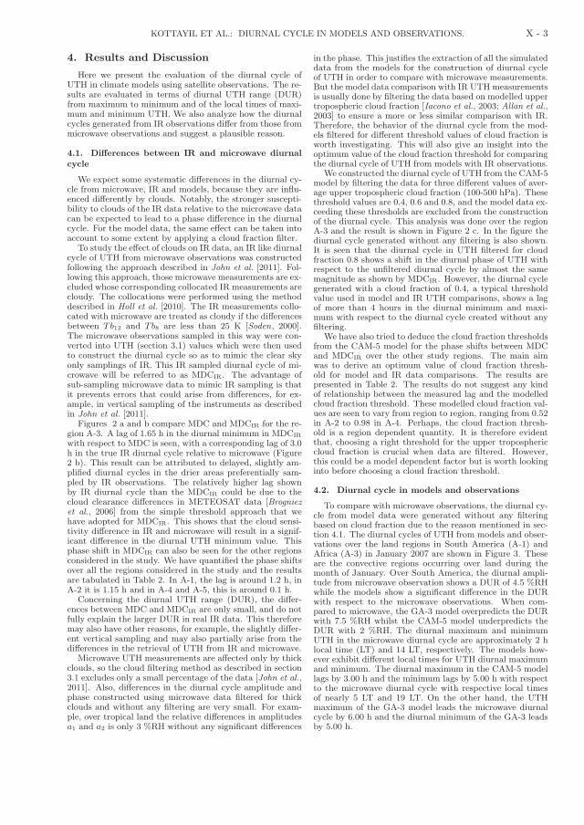
KOTTAYIL ET AL.: DIURNAL CYCLE IN MODELS AND OBSERVATIONS. X - 3
4. Results and Discussion
Here we present the evaluation of the diurnal cycle ofUTH in climate models using satellite observations. The re-sults are evaluated in terms of diurnal UTH range (DUR)from maximum to minimum and of the local times of maxi-mum and minimum UTH. We also analyze how the diurnalcycles generated from IR observations differ from those frommicrowave observations and suggest a plausible reason.
4.1. Differences between IR and microwave diurnalcycle
We expect some systematic differences in the diurnal cy-cle from microwave, IR and models, because they are influ-enced differently by clouds. Notably, the stronger suscepti-bility to clouds of the IR data relative to the microwave datacan be expected to lead to a phase difference in the diurnalcycle. For the model data, the same effect can be taken intoaccount to some extent by applying a cloud fraction filter.
To study the effect of clouds on IR data, an IR like diurnalcycle of UTH from microwave observations was constructedfollowing the approach described in John et al. [2011]. Fol-lowing this approach, those microwave measurements are ex-cluded whose corresponding collocated IR measurements arecloudy. The collocations were performed using the methoddescribed in Holl et al. [2010]. The IR measurements collo-cated with microwave are treated as cloudy if the differencesbetween Tb12 and Tb8 are less than 25 K [Soden, 2000].The microwave observations sampled in this way were con-verted into UTH (section 3.1) values which were then usedto construct the diurnal cycle so as to mimic the clear skyonly samplings of IR. This IR sampled diurnal cycle of mi-crowave will be referred to as MDCIR. The advantage ofsub-sampling microwave data to mimic IR sampling is thatit prevents errors that could arise from differences, for ex-ample, in vertical sampling of the instruments as describedin John et al. [2011].
Figures 2 a and b compare MDC and MDCIR for the re-gion A-3. A lag of 1.65 h in the diurnal minimum in MDCIR
with respect to MDC is seen, with a corresponding lag of 3.0h in the true IR diurnal cycle relative to microwave (Figure2 b). This result can be attributed to delayed, slightly am-plified diurnal cycles in the drier areas preferentially sam-pled by IR observations. The relatively higher lag shownby IR diurnal cycle than the MDCIR could be due to thecloud clearance differences in METEOSAT data [Brogniezet al., 2006] from the simple threshold approach that wehave adopted for MDCIR. This shows that the cloud sensi-tivity difference in IR and microwave will result in a signif-icant difference in the diurnal UTH minimum value. Thisphase shift in MDCIR can also be seen for the other regionsconsidered in the study. We have quantified the phase shiftsover all the regions considered in the study and the resultsare tabulated in Table 2. In A-1, the lag is around 1.2 h, inA-2 it is 1.15 h and in A-4 and A-5, this is around 0.1 h.
Concerning the diurnal UTH range (DUR), the differ-ences between MDC and MDCIR are only small, and do notfully explain the larger DUR in real IR data. This thereforemay also have other reasons, for example, the slightly differ-ent vertical sampling and may also partially arise from thedifferences in the retrieval of UTH from IR and microwave.
Microwave UTH measurements are affected only by thickclouds, so the cloud filtering method as described in section3.1 excludes only a small percentage of the data [John et al.,2011]. Also, differences in the diurnal cycle amplitude andphase constructed using microwave data filtered for thickclouds and without any filtering are very small. For exam-ple, over tropical land the relative differences in amplitudesa1 and a2 is only 3 %RH without any significant differences
in the phase. This justifies the extraction of all the simulateddata from the models for the construction of diurnal cycleof UTH in order to compare with microwave measurements.But the model data comparison with IR UTH measurementsis usually done by filtering the data based on modelled uppertropospheric cloud fraction [Iacono et al., 2003; Allan et al.,2003] to ensure a more or less similar comparison with IR.Therefore, the behavior of the diurnal cycle from the mod-els filtered for different threshold values of cloud fraction isworth investigating. This will also give an insight into theoptimum value of the cloud fraction threshold for comparingthe diurnal cycle of UTH from models with IR observations.
We constructed the diurnal cycle of UTH from the CAM-5model by filtering the data for three different values of aver-age upper tropospheric cloud fraction (100-500 hPa). Thesethreshold values are 0.4, 0.6 and 0.8, and the model data ex-ceeding these thresholds are excluded from the constructionof the diurnal cycle. This analysis was done over the regionA-3 and the result is shown in Figure 2 c. In the figure thediurnal cycle generated without any filtering is also shown.It is seen that the diurnal cycle in UTH filtered for cloudfraction 0.8 shows a shift in the diurnal phase of UTH withrespect to the unfiltered diurnal cycle by almost the samemagnitude as shown by MDCIR. However, the diurnal cyclegenerated with a cloud fraction of 0.4, a typical thresholdvalue used in model and IR UTH comparisons, shows a lagof more than 4 hours in the diurnal minimum and maxi-mum with respect to the diurnal cycle created without anyfiltering.
We have also tried to deduce the cloud fraction thresholdsfrom the CAM-5 model for the phase shifts between MDCand MDCIR over the other study regions. The main aimwas to derive an optimum value of cloud fraction thresh-old for model and IR data comparisons. The results arepresented in Table 2. The results do not suggest any kindof relationship between the measured lag and the modelledcloud fraction threshold. These modelled cloud fraction val-ues are seen to vary from region to region, ranging from 0.52in A-2 to 0.98 in A-4. Perhaps, the cloud fraction thresh-old is a region dependent quantity. It is therefore evidentthat, choosing a right threshold for the upper troposphericcloud fraction is crucial when data are filtered. However,this could be a model dependent factor but is worth lookinginto before choosing a cloud fraction threshold.
4.2. Diurnal cycle in models and observations
To compare with microwave observations, the diurnal cy-cle from model data were generated without any filteringbased on cloud fraction due to the reason mentioned in sec-tion 4.1. The diurnal cycles of UTH from models and obser-vations over the land regions in South America (A-1) andAfrica (A-3) in January 2007 are shown in Figure 3. Theseare the convective regions occurring over land during themonth of January. Over South America, the diurnal ampli-tude from microwave observation shows a DUR of 4.5 %RHwhile the models show a significant difference in the DURwith respect to the microwave observations. When com-pared to microwave, the GA-3 model overpredicts the DURwith 7.5 %RH whilst the CAM-5 model underpredicts theDUR with 2 %RH. The diurnal maximum and minimumUTH in the microwave diurnal cycle are approximately 2 hlocal time (LT) and 14 LT, respectively. The models how-ever exhibit different local times for UTH diurnal maximumand minimum. The diurnal maximum in the CAM-5 modellags by 3.00 h and the minimum lags by 5.00 h with respectto the microwave diurnal cycle with respective local timesof nearly 5 LT and 19 LT. On the other hand, the UTHmaximum of the GA-3 model leads the microwave diurnalcycle by 6.00 h and the diurnal minimum of the GA-3 leadsby 5.00 h.
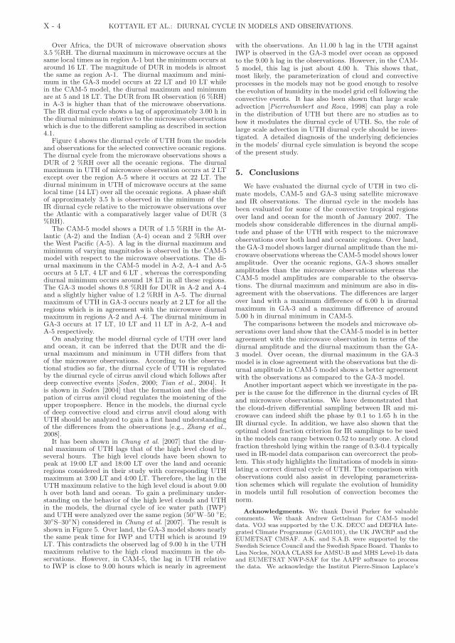
X - 4 KOTTAYIL ET AL.: DIURNAL CYCLE IN MODELS AND OBSERVATIONS.
Over Africa, the DUR of microwave observation shows3.5 %RH. The diurnal maximum in microwave occurs at thesame local times as in region A-1 but the minimum occurs ataround 16 LT. The magnitude of DUR in models is almostthe same as region A-1. The diurnal maximum and mini-mum in the GA-3 model occurs at 22 LT and 10 LT whilein the CAM-5 model, the diurnal maximum and minimumare at 5 and 18 LT. The DUR from IR observation (6 %RH)in A-3 is higher than that of the microwave observations.The IR diurnal cycle shows a lag of approximately 3.00 h inthe diurnal minimum relative to the microwave observationswhich is due to the different sampling as described in section4.1.
Figure 4 shows the diurnal cycle of UTH from the modelsand observations for the selected convective oceanic regions.The diurnal cycle from the microwave observations shows aDUR of 2 %RH over all the oceanic regions. The diurnalmaximum in UTH of microwave observation occurs at 2 LTexcept over the region A-5 where it occurs at 22 LT. Thediurnal minimum in UTH of microwave occurs at the samelocal time (14 LT) over all the oceanic regions. A phase shiftof approximately 3.5 h is observed in the minimum of theIR diurnal cycle relative to the microwave observations overthe Atlantic with a comparatively larger value of DUR (3%RH).
The CAM-5 model shows a DUR of 1.5 %RH in the At-lantic (A-2) and the Indian (A-4) ocean and 2 %RH overthe West Pacific (A-5). A lag in the diurnal maximum andminimum of varying magnitudes is observed in the CAM-5model with respect to the microwave observations. The di-urnal maximum in the CAM-5 model in A-2, A-4 and A-5occurs at 5 LT, 4 LT and 6 LT , whereas the correspondingdiurnal minimum occurs around 18 LT in all these regions.The GA-3 model shows 0.8 %RH for DUR in A-2 and A-4and a slightly higher value of 1.2 %RH in A-5. The diurnalmaximum of UTH in GA-3 occurs nearly at 2 LT for all theregions which is in agreement with the microwave diurnalmaximum in regions A-2 and A-4. The diurnal minimum inGA-3 occurs at 17 LT, 10 LT and 11 LT in A-2, A-4 andA-5 respectively.
On analyzing the model diurnal cycle of UTH over landand ocean, it can be inferred that the DUR and the di-urnal maximum and minimum in UTH differs from thatof the microwave observations. According to the observa-tional studies so far, the diurnal cycle of UTH is regulatedby the diurnal cycle of cirrus anvil cloud which follows afterdeep convective events [Soden, 2000; Tian et al., 2004]. Itis shown in Soden [2004] that the formation and the dissi-pation of cirrus anvil cloud regulates the moistening of theupper troposphere. Hence in the models, the diurnal cycleof deep convective cloud and cirrus anvil cloud along withUTH should be analyzed to gain a first hand understandingof the differences from the observations [e.g., Zhang et al.,2008].
It has been shown in Chung et al. [2007] that the diur-nal maximum of UTH lags that of the high level cloud byseveral hours. The high level clouds have been shown topeak at 19:00 LT and 18:00 LT over the land and oceanicregions considered in their study with corresponding UTHmaximum at 3:00 LT and 4:00 LT. Therefore, the lag in theUTH maximum relative to the high level cloud is about 9.00h over both land and ocean. To gain a preliminary under-standing on the behavior of the high level clouds and UTHin the models, the diurnal cycle of ice water path (IWP)and UTH were analyzed over the same region (50◦W–50 ◦E;30◦S–30◦N) considered in Chung et al. [2007]. The result isshown in Figure 5. Over land, the GA-3 model shows nearlythe same peak time for IWP and UTH which is around 19LT. This contradicts the observed lag of 9.00 h in the UTHmaximum relative to the high cloud maximum in the ob-servations. However, in CAM-5, the lag in UTH relativeto IWP is close to 9.00 hours which is nearly in agreement
with the observations. An 11.00 h lag in the UTH againstIWP is observed in the GA-3 model over ocean as opposedto the 9.00 h lag in the observations. However, in the CAM-5 model, this lag is just about 4.00 h. This shows that,most likely, the parameterization of cloud and convectiveprocesses in the models may not be good enough to resolvethe evolution of humidity in the model grid cell following theconvective events. It has also been shown that large scaleadvection [Pierrehumbert and Roca, 1998] can play a rolein the distribution of UTH but there are no studies as tohow it modulates the diurnal cycle of UTH. So, the role oflarge scale advection in UTH diurnal cycle should be inves-tigated. A detailed diagnosis of the underlying deficienciesin the models’ diurnal cycle simulation is beyond the scopeof the present study.
5. Conclusions
We have evaluated the diurnal cycle of UTH in two cli-mate models, CAM-5 and GA-3 using satellite microwaveand IR observations. The diurnal cycle in the models hasbeen evaluated for some of the convective tropical regionsover land and ocean for the month of January 2007. Themodels show considerable differences in the diurnal ampli-tude and phase of the UTH with respect to the microwaveobservations over both land and oceanic regions. Over land,the GA-3 model shows larger diurnal amplitude than the mi-crowave observations whereas the CAM-5 model shows loweramplitude. Over the oceanic regions, GA-3 shows smalleramplitudes than the microwave observations whereas theCAM-5 model amplitudes are comparable to the observa-tions. The diurnal maximum and minimum are also in dis-agreement with the observations. The differences are largerover land with a maximum difference of 6.00 h in diurnalmaximum in GA-3 and a maximum difference of around5.00 h in diurnal minimum in CAM-5.
The comparisons between the models and microwave ob-servations over land show that the CAM-5 model is in betteragreement with the microwave observation in terms of thediurnal amplitude and the diurnal maximum than the GA-3 model. Over ocean, the diurnal maximum in the GA-3model is in close agreement with the observations but the di-urnal amplitude in CAM-5 model shows a better agreementwith the observations as compared to the GA-3 model.
Another important aspect which we investigate in the pa-per is the cause for the difference in the diurnal cycles of IRand microwave observations. We have demonstrated thatthe cloud-driven differential sampling between IR and mi-crowave can indeed shift the phase by 0.1 to 1.65 h in theIR diurnal cycle. In addition, we have also shown that theoptimal cloud fraction criterion for IR samplings to be usedin the models can range between 0.52 to nearly one. A cloudfraction threshold lying within the range of 0.3-0.4 typicallyused in IR-model data comparison can overcorrect the prob-lem. This study highlights the limitations of models in simu-lating a correct diurnal cycle of UTH. The comparison withobservations could also assist in developing parameteriza-tion schemes which will regulate the evolution of humidityin models until full resolution of convection becomes thenorm.
Acknowledgments. We thank David Parker for valuablecomments. We thank Andrew Gettelman for CAM-5 modeldata. VOJ was supported by the U.K. DECC and DEFRA Inte-grated Climate Programme (GA01101), the UK JWCRP and theEUMETSAT CMSAF. A.K. and S.A.B. were supported by theSwedish Science Council and the Swedish Space Board. Thanks toLisa Neclos, NOAA CLASS for AMSU-B and MHS Level-1b dataand EUMETSAT NWP-SAF for the AAPP software to processthe data. We acknowledge the Institut Pierre-Simon Laplace’s

KOTTAYIL ET AL.: DIURNAL CYCLE IN MODELS AND OBSERVATIONS. X - 5
climate data service for facilitating the access of METEOSATdata.
References
Allan, R. P., M. A. Ringer, and A. Slingo (2003), Evaluationof moisture in the Hadley Centre climate model using sim-ulations of HIRS water-vapour channel radiances, QuarterlyJournal of the Royal Meteorological Society, 129, 3371–3389,doi:10.1256/qj.02.217.
Bodas-Salcedo, A., et al. (2011), COSP: satellite simulation soft-ware for model assessment, Bull. Amer. Met. Soc., 92, 1023–1043, doi:10.1175/2011BAMS2856.1.
Brogniez, H., R. Roca, and L. Picon (2006), A clear-sky radiancearchive from Meteosat “water vapor” observations, J. Geo-phys. Res., 111 (D10), D21109, doi:10.1029/2006JD007238.
Buehler, S. A., and V. O. John (2005), A simple method to re-late microwave radiances to upper tropospheric humidity, J.Geophys. Res., 110, D02110, doi:10.1029/2004JD005111.
Buehler, S. A., M. Kuvatov, and V. O. John (2005), Scan asym-metries in AMSU-B data, Geophys. Res. Lett., 32, L24810,doi:10.1029/2005GL024747.
Buehler, S. A., M. Kuvatov, T. R. Sreerekha, V. O. John,B. Rydberg, P. Eriksson, and J. Notholt (2007), A cloudfiltering method for microwave upper tropospheric humiditymeasurements, Atmos. Chem. Phys., 7 (21), 5531–5542, doi:10.5194/acp-7-5531-2007.
Buehler, S. A., M. Kuvatov, V. O. John, M. Milz, B. J. Soden,D. L. Jackson, and J. Notholt (2008), An upper tropospherichumidity data set from operational satellite microwave data,J. Geophys. Res., 113, D14110, doi:10.1029/2007JD009314.
Chung, E. S., B. J. Sohn, J. Schmetz, and M. Koenig (2007),Diurnal variation of upper tropospheric humidity and its re-lations to convective activities over tropical africa, Atmos.Chem. Phys., 7 (10), 2489–2502, doi:10.5194/acp-7-2489-2007.
Gettelman, A., W. D. Collins, E. J. Fetzer, A. Eldering, F. W.Irion, P. B. Duffy, and G. Bala (2006), Climatology of upper-tropospheric relative humidity from the atmospheric infraredsounder and implications for climate, J. Climate, 19 (23),6104–6121, doi:10.1175/JCLI3956.1.
Gettelman, A., H. Morrison, and S. J. Ghan (2008), A newtwo-moment bulk stratiform cloud micro- physics scheme inthe community atmosphere model, version 3 (cam3). part ii:Single- colunm and global results, J. Climate, 21, 3660–3679,doi:10.1175/2008jcli2116.1.
Gettelman, A., et al. (2010), Global simulations of ice nucle-ation and ice supersaturation with an improved cloud schemein the community atmosphere model, J. Geophys. Res., 115,doi:10.1029/2009jd013797.
Held, I. M., and B. J. Soden (2000), Water vapor feedback andglobal warming, Annu. Rev. Energy Environ., 25, 441–475.
Holl, G., S. A. Buehler, B. Rydberg, and C. Jimenez (2010), Col-locating satellite-based radar and radiometer measurements– methodology and usage examples, Atmos. Meas. Tech., 3,693–708, doi:10.5194/amt-3-693-2010.
Iacono, M. J., J. S. Delamere, E. J. Mlawer, and S. A. Clough(2003), Evaluation of upper tropospheric water vapor in theNCAR Community Climate Model (CCM3) using modeledand observed HIRS radiances, Journal of Geophysical Re-search (Atmospheres), 108, 4037, doi:10.1029/2002JD002539.
John, V. O., and B. J. Soden (2007), Temperature and humid-ity biases in global climate models and their impact on cli-mate feedbacks, Geophys. Res. Lett., 34, L18704, doi:10.1029/2007GL030429.
John, V. O., S. A. Buehler, and N. Courcoux (2006), A caution-ary note on the use of gaussian statistics in satellite basedUTH climatologies, IEEE Geosci. R. S. Le., 3 (1), 130–134,doi:10.1109/LGRS.2005.859350.
John, V. O., G. Holl, R. P. Allan, S. A. Buehler, D. E. Parker,and B. J. Soden (2011), Clear-sky biases in satellite infra-redestimates of upper tropospheric humidity and its trends, J.Geophys. Res., 116, D14108, doi:10.1029/2010JD015355.
John, V. O., G. Holl, N. Atkinson, and S. A. Buehler (2013),Monitoring scan asymmetry of microwave humidity soundingchannels using simultaneous all angle collocations (SAACs), J.Geophys. Res., doi:10.1029/2012JD018447, in press.
Kottayil, A., S. A. Buehler, V. O. John, L. M. Miloshe-vich, M. Milz, and G. Holl (2012), On the importanceof Vaisala RS92 radiosonde humidity corrections for a bet-ter agreement between measured and modeled satellite radi-ances, J. Atmos. Oceanic Technol., 29, 248–259, doi:10.1175/JTECH-D-11-00080.1.
Kottayil, A., V. O. John, and S. A. Buehler (2013), Correct-ing diurnal cycle aliasing in satellite microwave humiditysounder measurements, J. Geophys. Res., 118 (1), 101–113,doi:10.1029/2012JD018545.
MacKenzie, I. A., S. F. B. Tett, and A. V. Lindfors (2012),Climate Model-Simulated Diurnal Cycles in HIRS Clear-SkyBrightness Temperatures, Journal of Climate, 25, 5845–5863,doi:10.1175/JCLI-D-11-00552.1.
Miloshevich, L. M., H. Vomel, D. N. Whiteman, and T. Leblanc(2009), Accuracy assessment and correction of vaisala RS92radiosonde water vapor measurements, J. Geophys. Res., 114,D11,305, doi:10.1029/2008JD011565.
Neale, R. B., J. H. Richter, and M. Jochum (2008), The impactof convection on enso: from a delayed oscillator to a series ofevents, J. Climate, 21, 5904–5924, doi:10.1175/2008jcli2244.1.
Pierrehumbert, R. T., and R. Roca (1998), Evidence for controlof Atlantic subtropical humidity by large scale advection, Geo-phys. Res. Lett., 25, 4537–4540, doi:10.1029/1998GL900203.
Slingo, A., K. I. Hodges, and G. J. Robinson (2004), Simulationof the diurnal cycle in a climate model and its evaluation usingdata from Meteosat 7, Quarterly Journal of the Royal Meteo-rological Society, 130, 1449–1467, doi:10.1256/qj.03.165.
Soden, B. J. (2000), The diurnal cycle of convection, clouds, andwater vapor in the tropical upper troposphere, Geophys. Res.Lett., 27 (15), 2173–2176.
Soden, B. J. (2004), The impact of tropical convection and cir-rus an upper tropospheric humidity: A lagrangian analysis ofsatellite measurements, Geophys. Res. Lett., 31 (L20104), doi:10.1029/2004GL020980.
Soden, B. J., and F. P. Bretherton (1996), Interpretation of TOVSwater vapor radiances in terms of layer-average relative hu-midities: Method and climatology for the upper, middle, andlower troposphere, J. Geophys. Res., 101 (D5), 9333–9343, doi:10.1029/96JD00280.
Spangenberg, D. A., G. G. Mace, T. P. Ackerman, N. L. Seaman,and B. J. Soden (1997), Evaluation of model-simulated uppertroposphere humidity using 6.7 μm satellite observations, J.Geophys. Res., 102 (D22), 25,737–25,749.
Taylor, K. E., R. J. Stouffer, and G. A. Meehl (2012), AnOverview of CMIP5 and the Experiment Design, Bull. Amer.Met. Soc., 93, 485–498, doi:10.1175/BAMS-D-11-00094.1.
Tian, B., B. J. Soden, and X. Wu (2004), Diurnal cycle of con-vection, clouds, and water vapor in the tropical upper tropo-sphere: Satellites versus a general circulation model, J. Geo-phys. Res., 109, D10101, doi:10.1029/2003JD004117.
Walters, D. N., et al. (2011), The met office unified model globalatmosphere 3.0/3.1 and jules global land 3.0/3.1 configura-tions, Geoscientific Model Development, 4 (4), 919–941, doi:10.5194/gmd-4-919-2011.
Yang, G. Y., and J. Slingo (2000), The diurnal cycle in the trop-ics, Mon. Weather Rev.
Zhang, Y., S. A. Klein, C. Liu, B. Tian, R. T. Marchand, J. M.Haynes, R. B. McCoy, Y. Zhang, and T. P. Ackerman (2008),On the diurnal cycle of deep convection, high-level cloud,and upper troposphere water vapor in the Multiscale Mod-eling Framework, J. Geophys. Res., 113 (D12), D16105, doi:10.1029/2008JD009905.
Ajil Kottayil, Division of Space Technology, Department ofComputer Science, Electrical and Space Engineering, Lulea Uni-versity of Technology, Kiruna, Sweden, ([email protected])

X - 6 KOTTAYIL ET AL.: DIURNAL CYCLE IN MODELS AND OBSERVATIONS.
Figure 1. The mean UTH (%RH) values for the month of January 2007 from the CAM-5 model (see thetext for details). The black rectangles are the regions chosen for looking at the diurnal cycle of UTH frommodels and observations. The red bordered rectangle is the region selected for calibrating the satellitemeasurements from microwave data.
0 5 10 15 2040
41
42
43
44
45
46(a)
Local Time [hour]
UTH
[%R
H]
0 5 10 15 20−4
−3
−2
−1
0
1
2
3
4
(b)
Local Time [hour]
UTH
[%R
H]
0 5 10 15 20−4
−3
−2
−1
0
1
2
3
4
Local Time [hour]
UTH
[%R
H]
(c) cf−0.8cf−0.6cf−0.4
Figure 2. Left: The diurnal cycle of UTH generated from microwave measurements in January 2007using microwave sampling (black) and IR sampling (red) for the region A-3. See text for more details.Middle: The corresponding diurnal cycle fit, black line represents MDC and the red line is for MDCIR.The red dashed line represents the diurnal cycle from real IR data (for Januaries 1983–2005). Right:Diurnal cycle of UTH from CAM-5 model in January 2007 generated by filtering data for three differentupper tropospheric cloud fraction (cf) thresholds. The black curve represents the diurnal cycle generatedfrom all the simulated measurements.

KOTTAYIL ET AL.: DIURNAL CYCLE IN MODELS AND OBSERVATIONS. X - 7
0 5 10 15 20−5
−4
−3
−2
−1
0
1
2
3
4
5
Local Time [hour]
UTH
[%R
H]
A−1
MicrowaveCAMGA3
0 5 10 15 20−5
−4
−3
−2
−1
0
1
2
3
4
5
Local Time [hour]
UTH
[%R
H]
A−3
MicrowaveCAMGA3IR
Figure 3. The diurnal cycle of UTH from the models and observations for land regions in January 2007(Mean values are subtracted from UTH).
0 5 10 15 20−2
−1.5
−1
−0.5
0
0.5
1
1.5
2
Local Time [hour]
UTH
[%R
H]
A−2
MicrowaveCAMGA3IR
0 5 10 15 20−2
−1.5
−1
−0.5
0
0.5
1
1.5
2
Local Time [hour]
UTH
[%R
H]
A−4
MicrowaveCAMGA3
0 5 10 15 20−2
−1.5
−1
−0.5
0
0.5
1
1.5
2
Local Time [hour]
UTH
[%R
H]
A−5
MicrowaveCAMGA3
Figure 4. Same as Figure 3 but for oceanic regions.

X - 8 KOTTAYIL ET AL.: DIURNAL CYCLE IN MODELS AND OBSERVATIONS.
Figure 5. Diurnal cycle of UTH and IWP in January 2007 from models. The solid green line representsdiurnal cycle of UTH from GA-3 and the green dashed line is the IWP. The solid blue line (dashed blue)represents diurnal cycle of UTH (IWP) from the CAM-5 model.
Table 1. Geographical locations of the marked regions in Figure 1.
Region LocationSouth America (A-1) 40◦W–70 ◦W; 5◦–20◦SAtlantic (A-2) 10◦W–40 ◦W; 0◦–10◦NAfrica (A-3) 10◦E–40 ◦E; 0◦–20◦SIndian Ocean (A-4) 60◦E–90 ◦E; 0◦–15◦SWest Pacific (A-5) 110◦E–160 ◦E; 10◦N–10◦SSouth East Pacific (C-1) 70◦W–120 ◦W; 15◦–30◦S
Table 2. UTH diurnal cycle lag due to cloudiness. Column2: Measured lag in the diurnal phase in MDCIR
relative to MDC for different study regions. Column3: Corresponding cloud fraction threshold required to showthe same lag in CAM-5 model.
Region Measured lag (h) Model cf thresholdA-1 1.2 0.72A-2 1.15 0.52A-3 1.65 0.78A-4 0.1 0.98A-5 0.1 0.76Tropics (25◦S–25◦N) 1.55 0.56

The end.


