Repositioning and Market PowerAfter Airline Mergers∗

Sophia Li†, Joe Mazur‡, Yongjoon Park§, James Roberts¶,

Andrew Sweeting‖and Jun Zhang∗∗

June 2019

Abstract

We estimate a model of airline route competition in which carriers first choose

whether to offer nonstop or connecting service and then choose prices. Carriers have

full information about quality and marginal cost unobservables throughout the game,

so that carriers choosing nonstop service will be selected. Accounting for selection

when performing counterfactuals affects predictions about post-merger repositioning

by rivals, likely price increases and the effectiveness of remedies, and allows the model

to match observed changes after completed mergers.

Keywords: product repositioning, market power, endogenous market structure, selec-

tion, horizontal mergers, remedies, discrete choice games, multiple equilibria, airlines.

JEL Codes: C31, C35, C54, L4, L13, L93

∗We thank a number of discussants and seminar and conference participants for very useful comments.Fiona Scott Morton’s comments particularly helped to shape the motivation and presentation. The researchhas been supported by NSF Grant SES-1260876 (Roberts and Sweeting). Earlier versions of this paper werecirculated as “Airline Mergers and the Potential Entry Defense” and “Endogenous and Selective ServiceChoices After Airline Mergers”. Peichun Wang provided excellent research assistance during an early phaseof the project. Sweeting thanks the US Department of Justice for their hospitality while some of thisresearch was conducted, although the paper does not reflect the views or practice of the Department. Theusual disclaimer applies.†Li: Uber Technologies, ying.sophia@gmail.com.‡Mazur: Krannert School of Business, Purdue University, mazur3@purdue.edu.§Park: Department of Economics, University of Maryland, parky@econ.umd.edu.¶Roberts: Department of Economics, Duke University and NBER, jr139@duke.edu.‖Sweeting (corresponding author): Department of Economics, University of Maryland and NBER,

atsweet@umd.edu.∗∗Zhang: Department of Agricultural and Resource Economics, University of Maryland, zjun@umd.edu.

1

1 Introduction

Market power created by a horizontal merger may be limited if it induces new entry or

it prompts existing rivals to reposition to compete more directly with the merging firms.

Several court decisions at the end of the 1980s, including Waste Management, Baker Hughes

and Syufy1, indicated that the possibility of entry or repositioning should “trump” (Baker

(1996)) anti-competitive concerns unless barriers to entry would be higher for rivals than

they had been for the merging parties.

From an economic perspective, this approach was flawed because it did not ask whether

entry or repositioning would be profitable, and therefore likely to happen, or whether ei-

ther one would prevent prices from rising. In response, since 1992 the Horizontal Merger

Guidelines have laid out that the parties need to show that entry or repositioning will be

“timely, likely and sufficient” to prevent prices from rising (Shapiro (2010), p. 65). While

economists accept these criteria, they are rarely analyzed in a way comparable to how merger

simulations are used to quantify likely price changes with a fixed set of products. Instead,

as in the 1980s, court decisions and agency analysis continue to focus on barriers to entry or

repositioning without clear connections to profitability or price effects.2

We estimate a model of airline markets which integrates product positioning (a choice of

whether to provide nonstop or connecting service) and price-setting, and we use it to quantify,

in the spirit of the Guidelines, the likelihood and sufficiency of post-merger repositioning by

rivals, focusing on routes where the merging parties are both nonstop. Our model has

a standard two-stage structure where carriers make their service choices and then choose

prices. We assume that carriers know all of the demand (quality) and marginal cost shocks

that will affect second stage variable profits when making service choices, which we call the

“full information” assumption, and this gives rise to “selection” where a rival’s choice to

1United States v. Waste Management, Inc., 743 F.2d 976, 978, 983-84 (2d Cir. 1984), United States v.Baker Hughes Inc., 908 F.2d 981, 988-89 (D.C. Cir. 1990) and United States v. Syufy Enterprises, 903 F.2d659, 661 (9th Cir. 1990).

2For example, Coate (2008) describes the FTC’s conclusions about the likelihood of entry in internalmemoranda as lacking a “solid foundation” in the evidence, while Kirkwood and Zerbe (2009) classify onlyone of 35 post-1992 court opinions as reviewing the criteria in the Guidelines systematically. Some decisions,such as Oracle (331 F.Supp. 2d 1098 (N.D. Cal. 2004)) discuss new entry but are primarily decided on priorquestions of market definition.

2

provide connecting service pre-merger reflects, in part, the quality and costs that its nonstop

service would have. In contrast, most of the existing literature has assumed that firms only

learn demand and cost unobservables once entry or service choices have been made, because

this simplifies estimation. The computational burden of estimating a full information model

is reduced by using importance sampling, following Ackerberg (2009).

We view “full information” as the appropriate assumption when analyzing product repo-

sitioning by experienced market participants. It implies that carriers will not regret their

service choices in equilibrium, which is a desirable property if we want to understand whether

repositioning would continue to constrain market power in the medium-run.3 We perform

counterfactuals that account for the selection implied by pre-merger price and service choices,

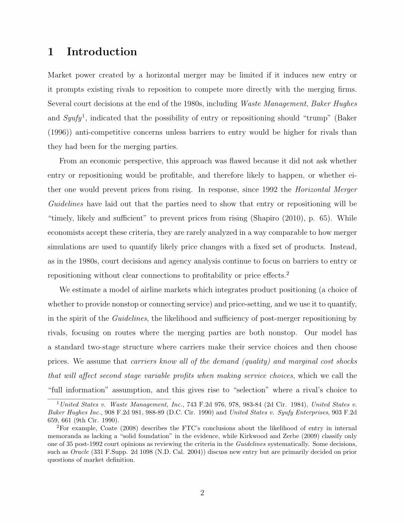
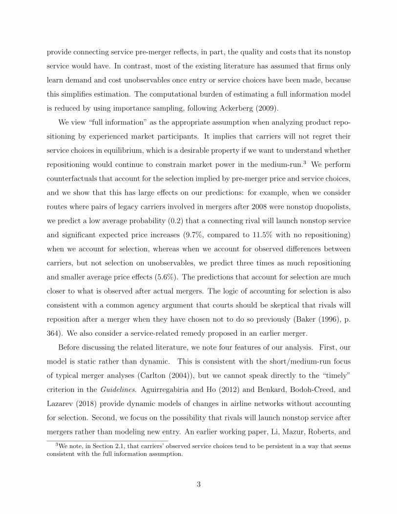
and we show that this has large effects on our predictions: for example, when we consider

routes where pairs of legacy carriers involved in mergers after 2008 were nonstop duopolists,

we predict a low average probability (0.2) that a connecting rival will launch nonstop service

and significant expected price increases (9.7%, compared to 11.5% with no repositioning)

when we account for selection, whereas when we account for observed differences between

carriers, but not selection on unobservables, we predict three times as much repositioning

and smaller average price effects (5.6%). The predictions that account for selection are much

closer to what is observed after actual mergers. The logic of accounting for selection is also

consistent with a common agency argument that courts should be skeptical that rivals will

reposition after a merger when they have chosen not to do so previously (Baker (1996), p.

364). We also consider a service-related remedy proposed in an earlier merger.

Before discussing the related literature, we note four features of our analysis. First, our

model is static rather than dynamic. This is consistent with the short/medium-run focus

of typical merger analyses (Carlton (2004)), but we cannot speak directly to the “timely”

criterion in the Guidelines. Aguirregabiria and Ho (2012) and Benkard, Bodoh-Creed, and

Lazarev (2018) provide dynamic models of changes in airline networks without accounting

for selection. Second, we focus on the possibility that rivals will launch nonstop service after

mergers rather than modeling new entry. An earlier working paper, Li, Mazur, Roberts, and

3We note, in Section 2.1, that carriers’ observed service choices tend to be persistent in a way that seemsconsistent with the full information assumption.

3

Sweeting (2015), estimated a model with both service choice and entry margins, but this

created a large computational burden for our prefered method of performing counterfactuals.

The reader should recognize, however, that our model can be applied to binary enter/do not

enter decisions in any market with a well-defined set of potential entrants (illustrated by

Monte Carlos in Li, Mazur, Park, Roberts, Sweeting, and Zhang (2018)). Third, we do

not model choices of route-level capacity or schedules, so some of the carrier heterogeneity

we find may reflect strategic scheduling choices.4 Finally, our baseline results assume that

service choices are made in a known, sequential order. This guarantees a unique equilibrium

outcome, and point identification. This choice provides tractability and we will explain in

detail why we believe it is reasonable below.

Section 2 describes our cross-sectional data and observed changes after mergers. Section

3 details the model, while Section 4 describes estimation. Section 5 presents the parameter

estimates. Section 6 presents our counterfactuals under different selection assumptions.

Section 7 concludes. The online Appendices provide supporting material.

Related Literature

The Civil Aeronautics Board and the Department of Transportation approved many airline

mergers in the 1980s, explicitly using arguments that entry or repositioning would prevent

incumbents from behaving anticompetitively (Keyes (1987)). Indeed, airlines was one of the

most cited industries during discussions of how entry and repositioning should fit into merger

analysis (Fisher (1987), Schmalensee (1987)). A reduced-form literature has estimated how

mergers affected prices after these mergers (summarized in Ashenfelter, Hosken, and Wein-

berg (2014)) and more recent ones (Huschelrath and Muller (2014), Huschelrath and Muller

(2015), Israel, Keating, Rubinfeld, and Willig (2013) and Carlton, Israel, MacSwain, and

Orlov (2017)). These retrospectives typically find that prices increased, but the results are

sensitive to the chosen control group and time-window.5 Surprisingly, these analyses have

4Park (2019) uses a model that includes capacity choices at one airport to address the effectiveness ofslot divestitures (rather then service remedies).

5For example, Borenstein (1990), Werden, Joskow, and Johnson (1991), Morrison (1996) and Peters(2006) find different signs for price effects after the 1986 TWA/Ozark and Northwest/Republic mergers.

4

not quantified post-merger entry or repositioning by rival carriers6, and retrospective studies

of the effectiveness of repositioning at constraining prices are also lacking in other industries.

The early literature on empirical discrete choice games, including Berry (1992) and Cilib-

erto and Tamer (2009) examining airlines, estimated reduced-form payoff functions without

modeling demand or pricing. Draganska, Mazzeo, and Seim (2009), Eizenberg (2014) and

Wollmann (2018) add models of price competition, but assume that firms have no informa-

tion on demand or marginal cost unobservables when making entry or service choices. This

type of “limited information” assumption implies that firms may regret their choices and

assumes away the type of selection that we study.

The most closely related papers are Reiss and Spiller (1989) and Ciliberto, Murry, and

Tamer (2018) (CMT, hereafter). Reiss and Spiller estimate a full information model of

service choice and price competition among airlines. They recognize “that entry introduces

a selection bias in equations explaining fares or quantities” (p. S201), but their analysis is

limited by imposing symmetry and allowing for at most one nonstop carrier.

CMT, developed contemporaneously with our paper, estimate a full information model

where carriers decide whether to enter and then compete on prices. There are, however,

important differences between the papers. CMT’s focus is on identification and estima-

tion allowing for multiple equilibria in a simultaneous-move entry game. Estimation uses

a nested fixed point (NFXP) approach and a supercomputer to minimize a discontinuous

objective function based on moment inequalities. Our assumptions rule out multiplicity

and we use importance sampling to generate a smooth objective function and to reduce

the computational burden. We argue that the sequential choice assumption, which provides

tractability, is reasonable when modeling service choices because we find that, once we con-

trol for observable market and carrier characteristics, two or more carriers appear marginal

for providing nonstop service, which is a necessary condition for more than one equilibrium

service choice outcome to exist, in only a relatively small proportion of markets. This is not

true for the entry choices that CMT analyze. We focus instead on counterfactual predic-

tions, and how they should be performed, motivated by a desire to provide a quantitative

6Huschelrath and Muller (2015) provides an analysis of entry in airline routes but without tying entry topre-merger market structures.

5

assessment of the criteria laid out in the Guidelines and because, in practice, the parameters

used in an investigation are often taken from documents or witness statements, rather than

being estimated.7

2 Data and Empirical Setting

We estimate our model using a cross-section of publicly-available DB1 (a 10% sample of

domestic itineraries) and T100 (records of flights between airports) data for the second

quarter of 2006. We use 2006 data so we can make predictions about subsequent mergers

and avoid later years when carriers have been alleged to price cooperatively (Ciliberto and

Williams (2014)). Appendix B complements this section with additional detail and analysis.

Market Selection and Carriers. We use data for 2,028 airport-pair markets linking the

79 busiest US airports in the lower 48 states. Excluded routes include short routes and routes

where nonstop service is limited by regulation. We model seven named carriers, American

Airlines, Continental Airlines, Delta Air Lines, Northwest Airlines, Southwest Airlines (a

low-cost carrier, LCC), United Airlines and US Airways, aggregating other ticketing carriers

into composite “Other Legacy” (primarily Alaska Airlines)8 and “Other LCC” (such as

JetBlue and Frontier) carriers. We attribute tickets and flights to mainline ticketing carriers

when they are operated by regional affiliates.

Service Types, Market Shares and Prices. We define the competitors on a route as

carriers ticketing at least 20 DB1 passengers and with at least a 1% market share (a one-way

passenger counts as half a return passenger). We define a carrier as nonstop if it has at least

64 T100 nonstop flights (5 flights per week) in each direction and at least 50% of its DB1

passengers do not make connections. The remaining competitors are connecting. The exact

level of these thresholds does not affect our classification. We model carriers as providing

7While CMT’s model implies selection, they use draws from their estimated distributions in their coun-terfactuals without requiring those draws to be consistent with pre-merger choices.

8Legacy carriers are carriers founded prior to deregulation in 1978, and they typically operate throughhub-and-spoke networks. Our classification of carriers as LCCs follows Berry and Jia (2010).

6

either connecting or nonstop service, not both. This is broadly consistent with the data: for

instance, less than 10% of passengers make connections for 80% of our nonstop carriers.

We model directional demand and pricing on each route, as a carrier’s presence at the

origin clearly affects a carrier’s market share.9 A carrier’s market share is calculated as the

total number of passengers that it carries, regardless of service type, divided by a measure of

market size. We define market size using an estimated gravity model (see Appendix B.1 and

Sweeting, Roberts, and Gedge (forthcoming)), accounting for total enplanements and route

distance. This measure is a better predictor of service choices, and it reduces unexplained

heterogeneity in market shares across routes and directions, compared with more common

measures based on average MSA populations. We measure a carrier’s price as the average

round-trip price in DB1. A measure of the proportion of business travelers on a route is

constructed based on data provided by Severin Borenstein (Borenstein (2010)).

Network Variables. We model route-level competition but recognize that network con-

siderations affect service choices. For instance, a carrier may find it profitable to serve a

segment nonstop because this generates traffic to other destinations. We capture these in-

centives by allowing the effective fixed cost of nonstop service to vary with whether the

endpoints include one of the carrier’s domestic or international hubs, and, for domestic hub

routes, with a continuous estimate of the quantity of connecting traffic that will be gener-

ated by nonstop service. The construction of this variable is detailed in Appendix B.2, and

while its calculation is not completely consistent with the strategic structure of our model,

it helps to explain service choices and it may approximate the type of measure that carriers

use internally to predict connecting passenger flows on new routes.

9Presence is defined by the number of nonstop routes that a carrier serves from an airport, divided bythe number of nonstop routes served by any carrier. Reduced-form analysis indicates that presence has largeeffects on demand. For example, in a route fixed effects regression, a one standard deviation increase inthe difference in a carrier’s presence across the endpoints increases the difference in the carrier’s directionalmarket shares by 20% of the average directional share, which may reflect frequent-flyers preferring to travelon one carrier. Differences in origin presence also have significant, although smaller, effects on directionaldifferences in average fares (Luttmann (2019)).

7

Table 1: Summary Statistics for the Estimation Sample

Numb. of 10th 90th

Obs. Mean Std. Dev. pctile pctile

Market VariablesMarket Size (directional) 4,056 24,327 34,827 2,794 62,454Num. of Carriers 2,028 3.98 1.74 2 6

Num. of Nonstop 2,028 0.67 0.83 0 2Total Passengers (directional) 4,056 6971 10830 625 17,545Nonstop Distance (miles, round-trip) 2,028 2,444 1,234 986 4,384Business Index 2,028 0.41 0.09 0.30 0.52

Market-Carrier VariablesNonstop 8,065 0.17 0.37 0 1Price (directional, round-trip $s) 16,130 436 111 304 581Share (directional) 16,130 0.071 0.085 0.007 0.208Airport Presence (endpoint-specific) 16,130 0.208 0.240 0.038 0.529Indicator for Low Cost Carrier 8,065 0.22 0.41 0 1≥ 1 Endpoint is a Domestic Hub 8,065 0.13 0.33 0 1≥ 1 Endpoint is an International Hub 8,065 0.10 0.30 0 1Connecting Distance (miles, round-trip) 7,270 3,161 1,370 1,486 4,996Predicted Connecting Traffic 1,036 8,664 7,940 2,347 52,726(at domestic hubs)

Table 2: Distribution of Market Structures in the Estimation Sample

Number of Nonstop Number of Percentage of Average Number ofCompetitors Sample Markets Sample Passengers Connecting Carriers

0 1,075 15.0% 3.981 614 33.6% 2.912 277 35.5% 2.073 60 15.2% 1.254 2 0.10% 0

2.1 Patterns in the Data

Market Structure and Service Types. Table 1 shows that markets have an average

of four carriers, with as many as nine on long routes, such as Orlando-Seattle, with many

plausible connecting airports. Most markets have no nonstop carriers but most passengers

travel in markets with at least two nonstop competitors (Table 2). These markets will be

the focus in our counterfactuals. Most of these routes connect large cities or hub airports,

but non-hub pairs such as Boston-Raleigh and Columbus-Tampa are also duopolies.10

10If we had defined markets using city-pairs, rather than airport-pairs, there would still be 192 duopolies(out of 1,533 city-pair markets), with 90 city-pair markets having three or more nonstop carriers.

8

The data clearly suggests that nonstop service has higher quality and that service choices

affect competition. Nonstop fares are $43 higher than connecting fares and, based on our

market definition, the average market share of a nonstop carrier is 18% compared to 4.9% for

a connecting carrier (small connecting carriers are already excluded). Controlling for route

characteristics, one nonstop carrier lowers connecting fares by $10, and a second nonstop

carrier lowers nonstop fares by $40 and connecting fares by an additional $30.11 LCC fares

are, on average, $70 lower than legacy fares, consistent with lower costs and/or quality.

Appendix B.3 shows that even simple functions of carrier and market variables explain

much of the variation in service choices. This informs how we design our service choice game

and how we think about identification. In 26% of markets the service choices of every carrier

are very close to being completely determined by observable variation (in the sense that

the predicted probabilities of nonstop service in a simple probit model are either less than

0.05 or greater than 0.95). For these observations, there should be (almost) no selection

on unobservables, so that conventional identification arguments for demand and marginal

cost equations, based on exclusion restrictions, should apply. A necessary (not sufficient)

condition for there to be multiple equilibrium service choice outcomes, whatever is assumed

about the timing of the service choice game, is that at least two carriers do not have dominant

service choice strategies. We find that there are only 24% of markets where two or more

carriers have nonstop choice probabilities between 0.05 and 0.95, implying that the number

of markets that may have multiple equilibria when we fit the model to the data may be

fairly small (outcomes where no carriers provide nonstop service will always be unique). We

therefore take the most tractable approach of estimating a game where there is always a

unique outcome, and we consider multiplicity primarily as a matter of robustness. We also

show in the Appendix that the patterns are quite different for the type of entry decision

modeled by Berry (1992), Ciliberto and Tamer (2009) and CMT (99% of markets have

at least two carriers with intermediate probabilities of “entry”), explaining why they find

multiple equilibria to be a standard feature of their estimates.

11These estimates are from regressions of a carrier’s weighted (across directions) average fare on a route onnonstop distance, carrier dummies, a dummy for whether the carrier provides nonstop service and interactionsbetween whether a carrier provides nonstop service and the number of nonstop carriers on a route.

9

Full Information. We assume that carriers know their qualities and costs when making

service choices. If, in contrast, carriers could only learn them by providing a particular type

of service, we might expect to observe brief periods of experimentation with different service

types. To test this, we have identified all cases where the named carriers added nonstop

service, other than through mergers, after Q1 2001 but before 2006, and then followed their

service choices over subsequent years. On average, these carriers maintained nonstop service

for 27 consecutive quarters, which seems too long to be consistent with experimentation

given that the industry received several negative demand shocks during these years.

What Happened To Service and Prices After Legacy Mergers? We use our model

to predict price and service changes after the Delta/Northwest (closed October 2008), United/

Continental (October 2010) and American/US Airways (December 2013) mergers that were

completed after our data. Appendix B.4 uses panel data to estimate what actually happened

after these mergers.

On routes where the merging carriers were nonstop duopolists, the merging parties always

maintained nonstop service. Within two years of the merger closing (the Department of

Transportation explicitly used two years when considering repositioning (Keyes (1987)), a

rival launched nonstop service on no routes, out of five, for Delta/Northwest, one route, out

of five, for United/Continental and three routes, out of six, for American/US Airways.12

There were two additional nonstop launches in the third years following these mergers. The

appendix also presents analyses of changes in the prices and market shares of the merging

firms on routes where the merging firms were nonstop duopolists for three years before the

merger, using a comparison set of routes where one of the parties was nonstop and the

other was either absent or a connecting carrier with a small share.13 On routes where no

rivals initiated nonstop service, we find that the merged carrier increased its prices by an

average of 10%, with its combined share of local traffic (i.e., passengers only flying the route

itself) falling by almost 30%. On routes where rival nonstop service was launched, prices

did not rise, although the merged firm did lose market share, presumably reflecting the

12There is no overlap in the routes across these mergers.13We recognize that results for price changes may be affected by using different control groups, as suggested

by the contrasting results in Huschelrath and Muller (2015) and Carlton, Israel, MacSwain, and Orlov (2017)for recent mergers.

10

new competition. These patterns suggest that rivals tend not to launch nonstop service

because they are poorly matched to providing nonstop service in these markets, rather than

because the merged carrier enjoys large synergies. Our baseline counterfactual assumptions

will assume that synergies are not realized, but we will also show that assuming one natural

form of synergies has only a small effect on our predictions.

3 Model

Consistent with most of the existing literature, we model carrier choices at the route-market

level. Consider a particular market, m, connecting two airports A and B. Carriers i =

1, ..., Im play a two-stage game, first choosing to provide nonstop or connecting service (a

binary choice) and then simultaneously choosing prices.

3.1 Second Stage: Post-Entry Price Competition

Given service choices, carriers play static, simultaneous Bertrand Nash pricing games for

passengers originating at each endpoint. Demand is determined by a nested logit model,

with all carriers in a single nest. For consumer k originating at endpoint A of route m, the

indirect utility for a return-trip on carrier i is

uA→Bkim = βA→Bim − αmpA→Bim + νm + τmζA→Bkm + (1− τm)εA→Bkim (1)

where pA→Bim is the price charged by carrier i for a return trip from A to B. The first term rep-

resents carrier quality associated with i’s service type (CON for connecting and NS for non-

stop), βA→Bim = βCON,A→Bim + βNSim x I(i is nonstop) with βCON,A→Bim ∼ N(XCONim βCON , σ

2CON)

and βNSim ∼ TRN(XNSim βNS, σ

2NS, 0,∞), so that quality can depend on observed carrier-

origin and route characteristics, and on a random component that is unobserved to the

researcher. TRN denotes a truncated normal distribution and the lower truncation of βNSim

at zero implies that the nonstop service is always preferred to connecting service on the

same carrier. Appendix C describes additional support restrictions imposed to estimate the

model. The price coefficient and nesting parameters are also heterogeneous across mar-

11

kets, with αm ∼ N(Xαβα, σ2α), where Xα will include the business index for the route, and

τm ∼ N(βτ , σ2τ ), although we assume that αm and τm are the same across directions.

νm, distributed N(0, σ2RE), is a route-specific random effect that is designed to capture the

fact that on some routes there are more travelers in both directions on most or all carriers,

relative to what independent quality draws can rationalize given our market size definition.

εA→Bkim is a standard logit error for consumer k and carrier i.

Each carrier has a marginal cost draw for each type of service. Specifically we assume that

cim ∼ N(XMCim βMC , σ

2MC), where XMC

im βMC allows costs to depend on the type of carrier, the

type of service and the distance traveled. For nonstop service we use the nonstop distance,

and for connecting service we use the distance via the connecting carrier’s closest domestic

hub.14 The marginal cost is non-directional as the representative traveler is assumed to

make a round-trip.

Our assumptions of nested logit demand, linear marginal costs and single product firms

imply that there will be unique equilibrium prices and directional variable profits, πA→Bim (s),

given service choices, cost and quality draws (Mizuno (2003)). i’s market-level variable

profits are πim(s) = πA→Bim (s) + πB→Aim (s), as service choices are assumed to be the same in

both directions.

3.2 First Stage: Service Type Choices

In the first stage carriers choose whether to commit to a fixed cost required for nonstop

service, or to provide connecting service. For our baseline estimation, we model carriers as

making their service choices sequentially in order of their average presence at the endpoints.

Their realized profits in the full game are therefore πim(s) − Fim x I(i is nonstop in m)

where Fim is a fixed cost draw associated with providing nonstop service. We assume

that Fim ∼ TRN(XFimβF , σ

2F , 0,∞), and, as emphasized in the Introduction, that all of the

market-level and carrier-level demand, marginal cost and fixed cost draws are known to all

carriers when they make service choices.

14For the composite Other Legacy and Other Low Cost carriers it is not straightforward to assign con-necting routes. Therefore we use the nonstop distance for these carriers, but include additional dummies inthe connecting marginal cost specification to provide more flexibility.

12

F should be interpreted as a net effective fixed cost. Providing nonstop service involves

committing gates and planes to a route, and these costs are fixed costs. However, a carrier

generates additional profits, in the form of connecting passengers going to or from other

destinations when it provides nonstop service, and we want F to reflect these additional

benefits, which is why we include our connecting traffic and network variables in XFim.15

Sequential choice ensures the existence of a unique subgame perfect Nash equilibrium,

and coupled with the assumed order, guarantees a unique predicted outcome. We will show

that our parameter estimates imply that there should be a unique outcome for almost all

market-draws even with different timing assumptions, and that the parameter estimates are

also very similar when we are agnostic about timing in estimation (Appendix C.7).

3.3 Solving the Model

Conditional on service choices, we solve for Nash equilibrium prices, shares and profits by

solving the system of pricing first-order conditions in the usual way. One can solve for

the outcome of the sequential service choice game by solving for profits given all possible

combinations of service choices and then using backwards induction. However, as we describe

in Appendix C.1, we solve for the equilibrium outcome more efficiently by selectively growing

the game tree forward, ignoring branches involving dominated choices.

3.4 Selection and Correlation in the Unobservables

Our baseline assumption is that the various demand and cost unobservables in our model are

independent. The type of selection that we are interested in arises from the fact that, under

full information, carriers choosing connecting service will tend to have worse (lower qual-

ity/higher cost) nonstop unobservables and may also tend to face rivals with better nonstop

unobservables. We show how accounting for this selection affects our counterfactuals, and

we allow for it by estimating the demand, pricing and service choice models simultaneously.

Richer correlations between service choices, prices and unobservables could arise if the

15Our specification does require that the net fixed cost is positive as this reduces the range of the importancedraws that we need to take. We show that this does not prevent us from accurately matching service choicesat major hubs.

13

demand and cost unobservables are themselves correlated. CMT allow for these correlations

in their model of airline entry, although they do not allow for cross-carrier correlations,

such as our νm. Our choice to assume independence for our baseline estimates primarily

reflects our experience that objective functions have multiple local minima when unrestricted

correlations are allowed, making us less confident in our estimates. However, our choice also

reflects the fact that our baseline estimates imply a limited role for cost unobservables (a

notable contrast to CMT) and that when we allow for correlations the best estimates that we

can find do not imply correlations that are clearly economically or statistically significant.16

4 Estimation

We minimize a simulated method of moments objective function of the formm(Γ, X)′Wm(Γ, X),

where W is a weighting matrix and Γ are the parameters. m(Γ, X) is a set of moments cal-

culated as 12,028

∑m=2,028m=1

(ydatam − Em(y|Γ, Xm)

)Zm, where subscript m denotes markets and

ym are observed price, share or service outcomes. Xm are observed variables, which are also

used to form the instruments, Zm.

We approximate the predictions of the model given the parameters, Em(y|Γ, Xm) using

importance sampling following Ackerberg (2009) (our application is closest to his example

2, albeit with a much richer model) to avoid resolving the model during estimation.17 The

idea is straightforward. Denoting a particular realization of all of the draws as θm,

Em(y|Γ) =

∫y(θm, Xm)f(θm|Xm,Γ)dθm

where y(θm, Xm) is the unique equilibrium outcome given our baseline assumptions. This

16We note that some of the large covariances that CMT estimate may reflect differences between nonstopand connecting service that we model or the additional controls that we include. We find that observedvariables generate significant correlations between demand and costs (see footnote 21).

17Ackerberg describes his approach as requiring a change of variables. The change is implicit in the waywe have written down our model. For example, in a traditional entry model a firm’s fixed cost might bewritten as Fi,m = Xi,mβF + uFi,m, and a NFXP estimation routine would integrate over the distribution ofthe us. An importance sampling approach requires a change of variables by taking draws of Fi,m rather thandraws of uFi,m. This is consistent with how we wrote down the model in terms of random draws of costs (e.g.,

Fim ∼ TRN(XFimβF , σ

2F , 0,∞)) and qualities in the previous section.

14

integral cannot be calculated analytically, but we can exploit the fact that

∫y(θm, Xm)f(θm|Xm,Γ)dθm =

∫y(θm, Xm)

f(θm|Xm,Γ)

g(θm|Xm)g(θm|Xm)dθm

where g(θm|Xm) is an “importance density” chosen by the researcher. This leads to a two-

step estimation procedure. In the first step we take many draws, indexed by s, from g(θm|Xm)

and solve for the equilibrium outcome, y(θms, Xm), for each of these draws. In the second

step we estimate the parameters, approximating Em(y) using

Em(y|Γ) =1

S

S∑s=1

y(θms, Xm)f(θms|Xm,Γ)

g(θms|Xm)

where we only need to recalculate f(θms|Xm,Γ) when the parameters change. An advantage

is that Em(y|Γ) is a smooth function of Γ even for discrete service choice outcomes. Our

reported estimates use 2,000 draws for each market, with S = 1, 000 used in estimation and

samples from the full pool of 2,000 used when estimating standard errors using a bootstrap

where markets are resampled. The computational burden is reasonable for academic research:

the first step takes less than two days on a medium-sized cluster, and the parameters are

estimated in one day on a laptop without any parallelization.

This approach assumes that g(θm|Xm) and f(θm|Xm,Γ) have the same support which

does not depend on Γ. Appendix C.2 details our chosen supports. We aim to include all

plausible values although this may reduce the accuracy of the approximation and potentially

lead to the estimates of the moment being inconsistent (Geweke (1989)), an issue we examine

in Appendix C.4.

Our baseline results use 1,384 moments, which reflect carrier service choices, prices and

market shares, and several market-level outcomes (such as the sum of squared market shares).

The Zs contain exogenous observed market, carrier and rival carrier characteristics. The

number of moments is large (relative to 2,028 market and 16,130 carrier-market-direction

observations), implying that estimates of the covariance of the moments may be inaccuarete.

We therefore use a diagonal weighting matrix, with equal weight on the groups of moments

associated with price, share and service choice outcomes and, within each group, the weight

15

on each moment is proportional to the reciprocal of the variance of that moment when

we estimated the model using an identity weighting matrix. Appendix C.6 shows that the

coefficients, fit and counterfactuals are very similar using a subset of 740 moments.

Identification. While all of our equilibrium and parametric assumptions contribute to

identification, the intuition is straightforward. The demand and marginal cost parameters

would be identified by exclusion restrictions if demand and marginal cost unobservables

were uncorrelated with service choices (i.e., no selection).18 Variation in service choices

with expected variable profits and the variables in XF would then identify the fixed cost

parameters. While our model allows for selection, Appendix B.3 shows that the service

choices in many markets are close to being determined by observables (for example, it is

almost certain that no carriers will be nonstop in small markets not involving hubs and that

a carrier will serve a large market from its hub nonstop). For these observations, there should

be essentially no selection on unobservables and conventional identification arguments apply.

5 Parameter Estimates

The first columns of Tables 3 and 4 present our baseline estimates. The demand coefficients

confirm several expected patterns: all else equal, consumers prefer nonstop service, legacy

carriers and carriers with greater originating airport presence. Demand is less elastic on

routes with more business travelers.19 The average own price demand elasticity is 4.25, and

the elasticity of demand for air travel (i.e., when all prices rise by the same proportion) is

1.3, consistent with literature averages reported by Gillen, Morrison, and Stewart (2003).

Implied diversion also illustrates the preference for nonstop service: in markets with two

nonstop carriers and at least one connecting carrier, a price increase by a nonstop carrier

leads to five times as many passengers switching to the other nonstop carrier as switch to

18For example, we assume that airport presence affects demand only at one endpoint of a route, thatdistance does affect marginal costs but does not affect connecting quality conditional on our definition ofmarket size, and that the business index only affects price sensitivity and preference for nonstop travel.MacKay and Miller (2018) show how our assumption of independence of demand and marginal cost shockscan identify demand even without exclusion restrictions. The market random effect will be identified bypositive correlations in market shares across firms and directions on the same route.

19The expected price coefficient (α) for Dayton-Dallas-Fort Worth, which has the highest business index,is -0.34 compared to the cross-market average of -0.57.

16

Table 3: Parameter Estimates: Demand

(1) (2) (3)Independent Correlation Correlation

Unobservables Specific. 1 Specific. 2Market-Level ParametersRandom Effect Std. Dev. σRE Constant 0.311 0.538 0.469

(0.138) (0.151) (0.122)Nesting Parameter Mean βτ Constant 0.645 0.634 0.640

(0.012) (0.013) (0.015)Std. Dev. στ Constant 0.042 0.005 0.050

(0.010) (0.010) (0.008)Demand Slope Mean βα Constant -0.567 -0.542 -0.612(price in $100 units) (0.040) (0.045) (0.031)

Business 0.349 0.189 0.435Index (0.110) (0.118) (0.088)

Std. Dev. σα Constant 0.015 0.043 0.013(0.010) (0.011) (0.013)

Carrier-Level ParametersCarrier Quality for Mean βCON Legacy 0.376 0.322 0.465Connecting Service Constant (0.054) (0.064) (0.047)

LCC 0.237 0.336 0.150Constant (0.094) (0.086) (0.094)Presence 0.845 0.674 0.524at Origin (0.130) (0.125) (0.127)

Std. Dev. σCON Constant 0.195 0.208 0.201(0.025) (0.027) (0.028)

Incremental Quality Mean βNS Constant 0.258 0.192 0.560of Nonstop Service (0.235) (0.214) (0.221)

Distance -0.025 -0.057 -0.009(0.034) (0.037) (0.036)

Business 0.247 0.841 -0.396Index (0.494) (0.455) (0.479)

Std. Dev. σNS Constant 0.278 0.241 0.213(0.038) (0.042) (0.034)

Notes: standard errors, in parentheses, are based on 100 bootstrap replications where 2,028 marketsare sampled with replacement, and we draw a new set of 1,000 simulation draws (taken from a poolof 2,000 draws) for each selected market. Distance is measured in thousands of miles. See Table 4for estimates of the cost and covariance parameters.

17

Table 4: Parameter Estimates: Marginal Costs, Fixed Costs and Covariances

(1) (2) (3)Independent Correlation Correlation

Unobservables Specific. 1 Specific. 2Carrier Marginal Costs Mean βMC Legacy 1.802 1.350 1.847($100 units) Constant (0.168) (0.146) (0.190)

LCC 1.383 0.961 1.344Constant (0.194) (0.169) (0.207)

Conn. X 0.100 0.443 0.040Legacy (0.229) (0.211) (0.251)

Conn. X -0.165 0.288 0.140(0.291) (0.255) (0.273)

Conn. X -0.270 -0.213 -0.228Other Leg. (0.680) (0.166) (0.160)

Conn. X 0.124 0.046 -0.173Other LCC (0.156) (0.152) (0.167)

Nonstop 0.579 0.823 0.510Distance (0.117) (0.101) (0.128)

Nonstop -0.010 -0.044 -0.001Distance2 (0.018) (0.016) (0.019)

Connecting 0.681 0.661 0.675Distance (0.083) (0.096) (0.091)

Connecting -0.028 -0.018 -0.026Distance2 (0.012) (0.013) (0.013)

Std. Dev. σMC Constant 0.164 0.191 0.143(0.021) (0.016) (0.018)

Carrier Effective Mean βF Legacy 0.887 0.897 0.855Fixed Costs Constant (0.061) (0.056) (0.063)

($1m. units) LCC 0.957 1.008 0.857Constant (0.109) (0.118) (0.100)

Dom. Hub -0.058 -0.302 -0.205Dummy (0.127) (0.157) (0.193)

Log -0.871 -1.000 -0.602(Conn. Traff.) (0.227) (0.207) (0.257)

Intl. Hub -0.118 -0.144 -0.107(0.120) (0.090) (0.093)

Slot Const. 0.568 0.424 0.514Airport (0.094) (0.099) (0.085)

Std. Dev. σF Constant 0.215 0.275 0.220(0.035) (0.029) (0.030)

Covariances Incremental Nonstop Quality - 0.012 0.018& Fixed Cost (0.010) (0.010)

Connecting Quality - - 0.006Marginal Cost (0.007)

Notes: see notes below Table 3. The Log(Predicted Connecting Traffic) variable is zero for routes thatdo not involve a domestic hub, and for hub routes it is re-scaled with mean 0.52 and standard deviation0.34.

18

connecting carriers.

Marginal costs are lower on LCCs and increase with distance. To illustrate, consider

the 3,000 mile round-trip Miami-Minneapolis route. For the named legacy carriers, the

expected nonstop marginal cost is $345, compared to an average of $367 for (longer-distance)

connecting service. Marginal costs for Southwest (and Other LCC) are lower and, for this

route, Southwest’s expected nonstop and connecting (via Chicago Midway) costs are almost

identical ($303 and $298 respectively). The expected effective fixed cost of nonstop service

is just over $840,000, but the expectation is lower ($610,000) for those carriers that choose

nonstop service because hub status and connecting traffic can reduce effective fixed costs

quite substantially: for example, a one standard deviation increase in connecting traffic

offsets almost $300,000 in fixed costs.

To assess the model fit and the importance of unobserved heterogeneity, we simulate 20

sets of all of the demand and cost variables for each market from the estimated distributions.

Observable variation accounts for the majority of variation in simulated costs: for example,

the standard deviation (across all carrier-market simulations) of Fi,m is $301, 912, and the

standard deviation of XFi,mβF is $259, 481, so that the unobserved heterogeneity provides only

14% of the variation. Similarly, it accounts for only 2.8% of the variation in marginal costs

and 15% of the variation in the price sensitivity of demand. Unobserved heterogeneity is more

important for carrier quality accounting for 26% of the variation in connecting quality and

34% of the variation in nonstop quality. The estimated σRE is also quite large and significant.

These patterns suggest that accounting for selection on carrier demand unobservables may

affect our counterfactuals.20

Our baseline estimates assume that carriers’ qualities and costs are only correlated

through observable variables and carriers’ choices.21 The remaining columns report esti-

mates when we allow up to two non-zero covariances between the unobservables. The esti-

20Li, Mazur, Park, Roberts, Sweeting, and Zhang (2018) uses these draws to estimate several linearprobability models to investigate how all of the observed and unobserved components of demand and costsaffect equilibrium service choices. Consistent with the simpler breakdown presented here, observables explainthe vast majority of variation in service choices, with demand unobservables playing a greater role than costunobservables.

21The observables create non-trivial correlations: for example, using same sets of draws, the correlationbetween a carrier’s nonstop quality and its fixed costs of nonstop service is -0.56, even though the unobservedcomponents are assumed to be independent.

19

mated covariances are small, and they are at most marginally significant. Even though we

can estimate covariances, we are more confident in our baseline estimates because we find

multiple local minima when we allow covariances.22 We will use the column (1) estimates in

our counterfactuals.

Our assumption of a known, sequential order of service choices guarantees a unique

outcome for all parameters. To see how restrictive this assumption is, we have examined

whether our estimates would support multiple outcomes if we allowed service choices to be

made simultaneously or in any different order. We find that multiplicity is rare: across

markets, the average number of outcomes that could be supported for a given set of draws

is only 1.017 (see Li, Mazur, Park, Roberts, Sweeting, and Zhang (2018), Table 4 for a

complete breakdown). Appendix C.7 presents another robustness check where we re-estimate

the parameters using moment inequalities making no assumptions about the timing of the

service choice game. Consistent with quality and cost draws only being able to support a

single outcome in most markets, which should be enough to provide point identification,

we find that a single set of coefficients minimizes the objective function and that these

coefficients are very similar to our baseline estimates.

5.1 Model Fit

We use our simulated draws to assess the fit of the model. We discuss predictions of service

choices here, with a discussion of prices and shares in Appendix C.5.

We predict a carrier’s observed service choice correctly for 87.5% of our draws (standard

error 1.1%). For 82.6% (2.2%) of carrier observations where the majority of our simulations

predict nonstop service, the carrier is nonstop in the data. Appendix Table C.3 shows that we

accurately predict that carriers will serve most routes from their hubs nonstop: for example,

we predict that Delta serves 92.5% (2.3%) of routes from Atlanta nonstop, compared to

96.5% in the data. We are also able to match service decisions where the link between

service choices and endpoint presence is less clear. To illustrate, Table 5 reports our service

choice predictions for routes involving Raleigh-Durham (RDU), a mid-sized non-hub airport.

The models predicts the proportion of routes served nonstop accurately for each carrier. The

22We have used grid searches to confirm that covariances near zero minimize the objective function.

20

Table 5: Model Fit: Predictions of Service Decisions at Raleigh-Durham

Number of Mean Presence at % NonstopRoutes Route Endpoints Data Simulation

American 44 0.29 22.7% 22.8% (1.6%)Continental 30 0.14 10.0% 10.0% (1.0%)Delta 57 0.24 8.7% 14.8% (1.9%)Northwest 22 0.18 9.1% 11.0% (1.2%)United 25 0.12 4% 14.4% (1.9%)US Airways 54 0.12 5.6% 9.4% (2.7%)Southwest 48 0.30 12.5% 14.5% (4.3%)Other Low Cost 25 0.08 4% 13.4% (4.9%)

Notes: Predictions from the model calculated based on twenty simulation drawsfrom each market from the relevant estimated distributions.

prediction is least accurate for United, as we usually predict that United should serve Denver

and San Francisco. United has launched nonstop service on both routes since 2006.

6 Merger Counterfactuals

We now present counterfactuals that predict post-merger repositioning and price changes,

illustrating how accounting for selection affects the predictions. We examine the three legacy

mergers completed after our sample and a blocked merger between United and US Airways

that was proposed in 2000. This merger is particularly interesting because the parties pro-

posed a remedy where a third carrier, American, would commit to provide nonstop service

for ten years on several routes where the merging parties were nonstop duopolists. This

would have preserved the number of nonstop alternatives for passengers and it would have

satisfied the likely and timely criteria in the Guidelines. However, the Department of Justice

viewed it as insufficient to constrain market power. Our model is well-suited to evaluating

this decision.23

23R. Hewitt Pate, Deputy Assistant Attorney General, discussed the merger and the remedy in a speech,“International Aviation Alliances: Market Turmoil and the Future of Airline Competition”, on November 7,2001, available at: https://www.justice.gov/atr/department-justice-10 (accessed June 29, 2017): “And thissummer, we announced our intent to challenge the United/US Airways merger, the second- and sixth-largestairlines, after concluding that the merger would reduce competition, raise fares, and harm consumers onairline routes throughout the United States and on a number of international routes, including giving Uniteda monopoly or duopoly on nonstop service on over 30 routes. We concluded that ... American Airlines’promise to fly five routes on a nonstop basis [was] inadequate to replace the competitive pressure that acarrier like US Airways brings to the marketplace, and would have substituted regulation for competition

21

Baseline Assumptions about the Merged Firm. A merger simulation requires making

assumptions about the quality and costs of the merged firm. Most of our analysis will

make a “baseline” assumption that the merged carrier (“Newco”) on each route will have

the quality and costs of the carrier with the higher average endpoint presence before the

merger. However, we can do the analysis under alternative assumptions, and we report

several results where the Newco is assumed to have the highest quality and lowest cost

draws of the merging parties even if these are from different carriers, which we will label the

“best case” assumption.24

6.1 Effects of Mergers Holding Service Types Fixed

We begin by calculating the predictions of the model when service types are held fixed, as is

typically done in merger simulations. We set the nesting and price coefficients equal to their

expected values for each market, infer carrier qualities and marginal costs from observed

market shares and prices, and then re-solve for post-merger prices, following Nevo (2000).25

The first panel of Table 6 reports results for routes where the merging parties are nonstop

duopolists under the baseline assumption about the merger. All of the mergers raise the

merging carriers’ average prices (we also take averages across directions), by between 5% and

15% (relative to their average pre-merger prices) with small standard errors. The market

share of the merging parties’ falls by between 25% and 30% reflecting both higher prices

and the elimination of a product. The next rows allow us to examine the profitability

of the merger. While the lack of synergies means that variable profits tend to fall, total

profits increase because a large fixed cost is eliminated. Connecting rivals also increase their

prices, although the magnitude of these changes are small. We measure consumer surplus

in dollars per pre-merger traveler, because our definition of the set of potential travelers is

likely imperfect and markets vary in size. Each merger is predicted to decrease consumer

on key routes. After our announcement, the parties abandoned their merger plans.”24The best case approach parallels what Li and Zhang (2015) assume about valuations and hauling costs

in the context of timber auctions. We use the label best case because it tends to increase the profits of themerging parties relative to our baseline assumption.

25Using the expected nesting and price coefficients reduces the computational burden when we endogenizeservice choices. The results are almost identical if this assumption is removed, consistent with the smallvariances of these parameters.

22

Tab

le6:

Pre

dic

ted

Eff

ects

ofM

erge

rsw

ith

Ser

vic

eC

hoi

ces

Hel

dF

ixed

Del

ta/N

ort

hw

est

Un

ited

/C

onti

nen

tal

Am

eric

an

/U

SA

irw

ays

Un

ited

/U

SA

irw

ays

Ave

rage

Dat

aP

ost

Data

Post

Data

Post

Data

Post

Data

Post

1.MergingPartiesNonstopDuopolists&

MergerEliminatesLower

Presence

Carrier

Nu

mb

.of

Rou

tes

2ro

ute

s4

rou

tes

11

rou

tes

7ro

ute

s24

rou

tes

Mer

gin

gC

arri

erP

rice

s$5

66.3

9$593.2

0(1.17)

$503.7

5$556.1

7(1.57)

$459.1

3$521.1

5(1.79)

$479.3

2$549.4

9(1.44)

$481.4

0$541.2

5(1.55)

Com

bin

edM

kt.

Sh

are

18.9

%14.3

%(0.1)

29.1

%21.

7%

(0.0)

26.9

%18.8

%(0.1)

20.8

%12.

9%

(0.0)

24.8

%17.

2%

(0.0)

Com

bin

edV

aria

ble

Pro

fit

($k)

1,28

7(4

7)

1,235

(43)

6,1

12

(208)

6,225

(208)

4,336

(201)

4,006

(187)

4,023

(124)

3,9

07

(104)

4,2

87

(164)

4,116

(151)

Com

bin

edF

ixed

Cos

ts($

k)

689

(108)

194

(55)

1,1

43

(144)

536

(66)

1,564

(90)

621

(47)

1,248

(100)

503

(61)

1,321

(96)

537

(51)

Ave

rage

Riv

alP

rice

s$2

35.9

0$237.

48

(0.10)

$455.5

7$457.2

9(0.03)

$400.4

4$404.1

8(0.14)

$280.1

9$282.0

9(0.15)

$360.8

5$363.5

3(0.08)

Ch

ange

inC

ons.

Su

rp.

Per

Tra

vele

r−

$51.3

6(1.64)

−$62.8

1(2.21)

−$64.0

6(2.89)

−$80.0

3(2.19)

−$67.0

4(2.47)

2.MergingPartiesNonstopDuopolists&

MergedFirm

ReceivesHighestQualities

andLowestCostsoftheMergingParties

Mer

gin

gC

arri

erP

rice

s$5

66.3

9$598.7

7(1.14)

$503.7

5$558.6

3(1.58)

$459.1

3$513.3

4(2.18)

$479.3

2$537.6

0(1.57)

$481.4

0$535.0

9(1.75)

Com

bin

edM

kt.

Sh

are

18.9

%15.1

%(0.0)

29.1

%21.

9%

(0.0)

26.9

%19.9

%(0.01)

20.8

%14.

3%

(0.0)

24.8

%18.

2%

(0.0)

Com

bin

edV

aria

ble

Pro

fit

($k)

1,28

7(4

7)

1,343

(414)

6,1

12

(208)

6,359

(209)

4,336

(201)

4,418

(162)

4,023

(124)

4,5

66

(103)

4,287

(164)

4,528

(141)

Com

bin

edF

ixed

Cos

ts($

k)

689

(108)

162

(39)

1143

(144)

375

(57)

1,564

(90)

565

(39)

1,248

(100)

446

(64)

1,321

(96)

465

(47)

Riv

alC

arri

erP

rice

s$2

35.9

0$237.

87

(0.06)

$455.5

7$457.1

4(0.03)

$400.4

4$403.4

6(0.14)

$280.1

9$281.3

6(0.04)

$360.8

5$362.9

1(0.08)

Ch

ange

inC

ons.

Su

rp.

Per

Tra

vele

r−

$44.8

8(1.72)

−$60.8

3(2.18)

−$56.9

4(3.21)

−$68.2

5(2.19)

−$59.7

4(2.63)

3.Alternative

Market

Structures&

MergerEliminatesLower

Presence

Carrier

Mer

gin

gp

arti

esn

onst

op$3

51.2

6$382.0

4$438.0

8$464.9

8$363.1

1$404.8

4$350.0

2$378.1

5$368.7

0$402.0

8w

ith

non

stop

riva

ls2

rou

tes

4ro

ute

s10

rou

tes

10

rou

tes

26

rou

tes

On

ep

arty

non

stop

,$4

72.9

9$524.6

7$502.6

0$513.2

9$447.9

5$478.9

5$443.3

0$462.5

3$458.0

2$486.4

0ot

her

con

nec

tin

g91

rou

tes

59

rou

tes

158

rou

tes

163

rou

tes

471

rou

tes

Bot

hp

arti

esco

nn

ecti

ng

$433

.26

$444.6

3$487.0

4$486.8

6$464.2

0$457.7

7$484.2

5$479.6

2$466.0

0$465.9

747

9ro

ute

s334

route

s471

rou

tes

521

rou

tes

1,8

05

rou

tes

Not

es:

for

rou

tes

wh

ere

the

mer

gin

gca

rrie

rsar

en

on

stop

du

op

oli

sts,

stan

dard

erro

rsfo

rm

easu

res

not

dir

ectl

yob

serv

edin

the

data

are

rep

ort

edin

pare

nth

e-se

s,an

dth

esh

are,

fixed

cost

and

pro

fit

nu

mb

ers

are

for

the

mer

gin

gca

rrie

rsco

mb

ined

.P

rice

sav

eraged

acr

oss

dir

ecti

on

s,an

dp

re-m

erger

pri

ces

are

aver

ages

acro

ssca

rrie

rs.

For

other

pre

-mer

ger

mar

ket

stru

ctu

res,

the

tab

lesh

ows

the

nu

mb

erof

aff

ecte

dro

ute

s,an

dm

ergin

gca

rrie

rp

rice

sw

ith

no

stan

dard

erro

rs.

All

calc

ula

tion

sas

sum

eth

atth

ep

rice

and

nes

tin

gp

ara

met

ers

hav

eth

eir

exp

ecte

dva

lues

for

each

mark

et.

Each

mer

ger

isco

nsi

der

edse

para

tely

,n

ot

cum

ula

tivel

y.

23

surplus significantly, as one of the largest firms is eliminated and the other is raising its price

significantly.

The second panel shows the results under the best case merger assumption. The numbers

change in the expected directions: the merged firm is expected to lose fewer passengers, and

its profits increase. However, the changes are relatively small: for example, the merged

firm’s prices increase by 11.2% rather than 12.4% under the baseline assumption. This is

because the higher presence carrier, which survives in the baseline case, tends to have higher

observed quality and the random elements of quality and costs tend to be too small to create

substantial differences.26

The third panel reports pre- and post-merger average prices for the merging firms under

our baseline merger assumption for different market structures (we do not report standard

errors to prevent excessive clutter, but the predictions are also precise). When the merging

parties are both nonstop, but face additional nonstop rivals, predicted price increases are

substantial (average 9.1%), and we will consider these markets in later counterfactuals. When

one party is nonstop and the other is connecting we tend to predict smaller increases (6.1%),

although they are quite large for Delta/Northwest routes where the connecting party often

has an unusually high market share. When both parties are connecting we predict small

price reductions, which is possible when the higher presence carrier has lower costs because

its connecting hub is more conveniently located. Consumer surplus still falls because the

disappearance of an option, but the drop is much smaller than for nonstop duopolies (average

$4.91 per pre-merger traveler).

6.2 Merger Counterfactuals When Rivals’ Service Types Can Change

We now present counterfactuals where rival service choices are allowed to change after a

merger. We describe how we create distributions for connecting carriers’ nonstop qualities

and costs, before presenting our predictions and our analysis of potential service remedies.

26In contrast CMT estimate that unobserved carrier quality and costs are more important, and thatdifferent merger assumptions change counterfactual predictions quite dramatically.

24

Conditional Distributions. Merger simulations that assume fixed entry or service types

use firm qualities and marginal costs that are consistent with observed pre-merger market

shares and price choices, as well as estimates of demand. When allowing service types

to change, it is therefore natural to use qualities and costs for the service types that are

not chosen pre-merger that are also consistent with pre-merger service choices, as well as

the estimated parameters, even if these qualities and costs cannot be pinned down exactly.

By doing so, we can account for the selection implied by equilibrium pre-merger choices.

We form distributions for these unobserved qualities and costs, which we call conditional

distributions, although one can interpret them as posteriors if the estimated distributions

are treated as priors.

The conditional distributions are formed using simulation with the following steps. First,

we specify a discrete set of possible values for the market-level demand random effect. For

each value, we calculate the qualities and marginal costs implied by observed prices and

market shares for the chosen service types. We then take draws of the remaining random

components of the model from their estimated distributions and, for each set of draws, we

check whether the observed service choices would be an equilibrium outcome of the sequential

service choice game, keeping the accepted draws. We weight the accepted draws using the

estimated distribution of the random effect, and the density of observed qualities and costs,

to form the conditional joint distribution of the random effect, carrier qualities, marginal

costs and fixed costs for all of the carriers in the market.27

We illustrate the effect of conditioning in Figure 1 for the Philadelphia (PHL)-San Fran-

cisco (SFO) market, one of the nonstop duopoly markets affected by the United/US Airways

merger. The solid line in the left panel shows the estimated density of the demand random

effect, while the histogram shows the simulated marginal conditional density (50,000 simu-

lation draws). The conditional distribution has a lower mean, reflecting the fact that the

number of observed passengers, across all carriers, is relatively low (combined market share

is 28.3%, averaged across directions) given the value of the observed covariates, including

our market size variable. As a comparison, the mean of the conditional distribution for Las

27The acceptance rate drops if more discrete choices are added to the model or we add additional players.This is the primary reason why we moved away from the Li, Mazur, Roberts, and Sweeting (2015) modelwhere we gave carriers three choices (do not enter, enter connecting, enter nonstop).

25

Figure 1: Selection of Marginal Conditional Distributions for Philadelphia-San Francisco

-1 -0.5 0 0.5 1

Value of Market Random Effect

0

0.5

1

1.5

2

2.5

3

3.5

4

4.5

5

pdf

Random Effect Distributions

EstimatedConditional

-1 0 1 2 3

Nonstop Quality

0

0.2

0.4

0.6

0.8

1

1.2

1.4

1.6

1.8Nonstop Qualities from SFO

United EstimatedAmerican EstimatedAmerican Conditional

0 0.5 1 1.5 2

Fixed Costs ($s) 106

0

0.5

1

1.5

2

10 -6 Nonstop Fixed Costs

US Airways EstimatedAmerican EstimatedAmerican Conditional

Vegas-Miami, where combined market shares equal 42.5%, is 0.5.

Nonstop quality is the sum of a carrier’s connecting quality and the incremental quality

of nonstop service. The solid lines in the middle panel show the density of nonstop quality

for passengers originating at SFO for United and American based on the estimates. United’s

expected quality is higher, because of its high presence at SFO. The histogram shows the

conditional density for American’s nonstop quality. This distribution is similar, but with

a slightly lower mean, than the distribution implied by the estimates. The intuition is

that given observed shares and prices and the likely value of the random effect, we only

need to shift our belief about American’s quality down by a small amount to explain why

it chooses connecting service. The third panel shows the marginal densities for the fixed

cost of nonstop service for American and US Airways. US Airways has a lower expected

effective fixed cost because of its domestic and international hubs at PHL. The estimated

and conditional distributions for American’s fixed costs look essentially identical.

26

Table 7: Predicted Effects of United/US Airways Merger in Four Nonstop Duopoly MarketsWhere American is a Connecting Competitor using Conditional Distributions for ConnectingCarriers’ Nonstop Quality and Costs

Pre-Merger Exp. Numb. of Rivals Post-Merger Change inService Change United/US Launching Nonstop Service Merged Carrier ConsumerConsidered Airways Price American Other Rivals Price Surplus

Baseline Merger Assumption1. Service Types $531.97 - - $577.72 -$48.07Fixed (0.76) (1.69)2. Rivals’ Choices $531.97 0.035 0.063 $573.37 -$42.96Endogenized (0.023) (0.055) (2.36) (4.88)

Best Case Merger Assumption1. Service Types $531.97 - - $562.82 -$37.76Fixed (0.94) (1.77)2. Rivals’ Choices $531.97 0.020 0.043 $560.73 -$33.80Endogenized (0.015) (0.042) (1.96) (4.00)

Notes: predictions are averages across 1,000 draws from the conditional distributions. In the base-line case, the merger eliminates the carrier with the lowest presence on the route. Standard errors inparentheses based on the same bootstrap estimates used for the parameter estimates. The reportedpre-merger price is the average of the merging carriers’ prices across directions. Consumer surpluschanges measured per pre-merger traveler. For American, the expected number of rivals launchingnonstop service is the probability that American launches nonstop service.

Predicted Effects of a United/US Airways Merger Using the Conditional Distri-

butions. We now present our predictions of what would have happened after the United/US

Airways merger when we endogenize service choices and ensure that our assumptions are

consistent with pre-merger choices. We focus on four routes where the merging parties were

nonstop duopolists and American provided connecting service, so we can later consider the

effects of the American nonstop remedy. We note that it is not unusual for merger analyses

to focus on a small number of markets, but below we will consider 17 additional nonstop

duopoly routes when we examine the completed mergers.

The upper panel in Table 7 presents some summary results under our baseline merger

assumption. We expect the merged firm’s prices to increase by 8.6% on these routes if

service types are held fixed with a significant predicted decline in consumer surplus. These

predictions would usually lead an antitrust agency to oppose a merger unless offsetting

synergies or repositioning are likely.

The second row reports our predictions when we allow rivals’ service types to change

27

after the merger, using 1,000 draws from the conditional distributions for each market.

We impose that the merged firm maintains nonstop service, as this is always observed in

the data.28 The connecting rivals re-optimize their service choices, in the order assumed

in estimation. The expected number of rivals initiating nonstop service, a measure of the

likelihood of repositioning, is small: across the four markets, American (another rival) does

so for only 3.5% (6.3%) of simulations, leading to the result that, in expectation, the merged

carrier’s price increases by $41 (7.8%), so the possibility of repositioning is not sufficient to

constrain prices. We also find that the merger is, on average, profitable for the merging firm

despite the repositioning that takes place, with its profits increasing by an average of $279k

(s.e. $78k) per market.

The lower panel performs the same simulations under the best case assumption. As

expected, this results in smaller predicted price increases and smaller declines in consumer

surplus, with less repositioning by rivals. However, as when service types are held fixed, the

magnitudes of the changes are small, except that the merger is now predicted to raise profits

by $1.1m. (s.e. $85k).

To understand what happens, Table 8 provides more detail for the PHL-SFO market

under the baseline assumption. This is the market most affected by repositioning because,

prior to the merger, the lower presence (eliminated) party, United, has a large market share.

We use 5,000 draws for this analysis so we can measure different outcomes accurately.

For two-thirds of the draws, no connecting rival launches nonstop service, and merged

carrier’s price increases by 9.5% (from the pre-merger average) and its market share falls by

38%. The non-merging carriers, with small shares pre-merger, increase their prices slightly

and double their combined market share. Reflecting the loss of a large carrier, consumer

surplus falls by an average of $72.91 per pre-merger traveler.

The remaining columns show what happens when one of American or Delta launch non-

stop service, which are the most common outcomes involving repositioning (for 0.9% of

draws more than one rival launches nonstop service). The increased competition reduces

(but does not eliminate) the equilibrium price increase for US Airways, but the new nonstop

28This is almost always the equilibrium outcome with conditional distributions, but it is frequently notthe predicted outcome when we use alternative distributions, which provides an additional reason why thesealternatives are less reasonable.

28

Table 8: Predictions for the Philadelphia-San Francisco Market Allowing for EndogenousRival Service Choices Following a United/US Airways Merger

Carrier No Service Changes American Nonstop Delta Nonstop

(pre-merger service type, 3,267/5,000 Draws 570/5,000 Draws 483/5,000 Drawsprice and share) Price Share Price Share Price Share

US Airways/Newco $691.53 15.4% $661.67 14.1% $661.46 14.0%(NS, $649.74, 13.0%) (1.17) (0.0) (0.66) (0.1) (1.64) (0.1)

United - - - - - -(NS, $613.54, 12.1%)

American $478.98 1.2% $554.64 8.1% $477.30 0.8%(CON, $476.52, 0.5%) (0.05) (0.0) (9.70) (0.4) (0.07) (0.0)

Delta $666.89 0.6% $666.08 0.4% $550.98 7.9%(CON,$665.77,0.3%) (0.03) (0.0) (0.04) (0.0) (8.74) (0.5)

Northwest $307.35 3.5% $302.51 2.4% $302.47 2.4%(CON, $300.60,1.9%) (0.18) (0.0) (0.23) (0.1) (0.23) (0.1)

Other LCC $377.27 1.1% $375.82 0.7% $375.80 0.7%(CON,$375.27,0.6%) (0.06) (0.0) (0.07) (0.0) (0.07) (0.0)

Notes: predictions are averages from 5,000 draws from the conditional distributions. Standard er-rors in parentheses based on the same bootstrap estimates used for the parameter estimates. Themerger assumed to eliminate United (lower presence carrier). NS denotes nonstop and CON de-notes connecting pre-merger.

carrier usually has a market share that is smaller than United’s prior to the merger, causing

consumer surplus to fall by around $30 per pre-merger traveler in both cases. Repositioning

by rivals, when it happens, does tend to make the merger unprofitable for this route: for

example, the merged firm’s profits fall by $920k when American becomes nonstop.29

Predicted Effects Using Alternative Assumptions About Rival Qualities. Rows

3 and 4 of the upper panel of Table 9 presents the summary results for the four routes using

two alternative types of assumption about the nonstop qualities and costs of connecting

rivals. To save space, we do not report standard errors in the remaining tables, but they

are of similar magnitude to those reported earlier and we will note in the text where any

discussed changes are not statistically significant.

The first alternative (row 3) uses new draws from the estimated cost and incremental

29We have also calculated what happens under the best case assumption. In this case, there is no reposi-tioning for 78% of draws (rather than 65%), US Airways price increases by an average of 4.3% (rather than6.4%) when there is no repositioning and the merger is only marginal unprofitable when repositioning occurs(e.g., profits fall by $106k when American becomes nonstop).

29

Table 9: Predicted Effects of United/US Airways Merger in Four Nonstop Duopoly MarketsUnder the Baseline Merger Assumption Using Different Assumptions About the Nonstop Qualityand Costs of Rivals, And Allowing for the American Service Remedy

Pre-Merger Exp. Numb. of Rivals Post-Merger Change inService Change United/US Launching Nonstop Service Merged Carrier ConsumerConsidered Airways Price American Others Price Surplus

1. No Service Changes $531.97 - - $577.72 -$48.07Allow Rival Service Changes

Counterfactuals Computed Using2. Conditional Distns. $531.97 0.035 0.063 $573.37 -$42.96

3. Estimated Distns. $531.97 0.190 0.325 $559.56 -$16.22

4. Connecting Carriers’ $531.97 0.678 1.915 $531.79 +$62.36Nonstop Same as Average Merging Parties

American Nonstop Remedy Allowing Rival Service Changes

5. Conditional Distns. $531.97 1 0.030 $566.34 -$31.29

6. Estimated Distns. $531.97 1 0.253 $556.18 -$3.98

7. Connecting Carriers’ $531.97 1 1.883 $529.90 +$68.55Nonstop Same as Average of Merging Parties

Notes: predictions with endogenous service choices are averages from 1,000 draws from the appropriatedistributions. The merger is assumed to eliminate the carrier with the lowest presence on the route.Implementation of rows 3 and 4 explained in the text. Standard errors not reported (referenced whererelevant in the text).

nonstop quality distributions for the nonstop qualities and costs of the connecting carriers

(which parallels the approach of CMT). We therefore account for differences in the observable

characteristics of different carriers, but do not account for the additional information in pre-

merger service choices. The second alternative (row 4) assumes that if any connecting rival

becomes nonstop then it would have the average quality and marginal costs of the merging

nonstop carriers and draw its fixed cost from a distribution that has a mean equal to average

of the means for the merging carriers. This approach ignores observable differences between

firms, but it might be viewed as being consistent with the logic of Waste Management and

the Department of Transportation’s decisions if clear barriers to repositioning could not

be identified. In both cases, we continue to draw the random effect from its conditional

distribution and we use the qualities and marginal costs for observed service types that are

implied by observed prices and market shares.30

30The rationale for using the conditional distribution of the random effect is that its role is to addressimperfections in our definition of market size, and, in a merger investigation, the parties and the agencieswould likely be able to construct better measures of potential demand.

30

Using the estimated distributions significantly increases the probability that rivals will

launch nonstop service (the expected number of nonstop launches is 0.52, rather than 0.1),

leading to a smaller expected price increase and a decrease in consumer surplus of $16.22

per pre-merger traveler that is not statistically significant (s.e. $11.22). The merger is, on

average, unprofitable: profits fall by an average of $105k (s.e. $150k), whereas they increase

by $279k (s.e. $78k) when we use the conditional distributions.

Assuming that connecting carriers can offer nonstop service on similar terms to the merg-

ing parties leads to a prediction that, on average, 2.6 of them would launch nonstop service31

and that, because more firms tend to have significant market shares, consumer surplus in-

creases after the merger. However, if we use the same assumption to solve for equilibrium

outcomes before the merger, we would predict that several connecting carriers should have

chosen to offer nonstop service (e.g., American’s probability of launching nonstop service

would be 0.6 pre-merger), which is inconsistent with the observed data. This highlights the

importance of trying to assess whether assumptions about the post-merger competitiveness

of repositioning firms, or new entrants, are consistent with their pre-merger choices. The

results are similar if we make the best case merger assumption: for example, the expected

number of carriers launching nonstop service are 0.46 (row 3) and 2.4 (row 4), rather than

0.52 and 2.6.

The Proposed Service Remedy. The results presented so far suggest that when rivals

launch nonstop service, the merging firms will only increase prices by a small amount. This

might be interpreted as implying that the proposed American nonstop remedy, which would

have maintained the number of nonstop carriers at its pre-merger level, would have been

effective. However, this logic implicitly assumes that American’s nonstop service would

constrain the merged carrier’s prices even when it is unprofitable.32

The lower panel of Table 9 presents our average predictions for the four routes using

the different distributions when we force the merged firm and American to provide nonstop

31If we assumed that connecting carriers would be similar to the eliminated carrier, rather than the averageof the merging carriers, we would expect 1.5 of them to launch nonstop service.

32The parties did not claim that nonstop service on the affected routes would be profitable for American:instead the attraction for American was that it would receive a package of assets on the East Coast if themerger was completed.

31

service, but allow other carriers to sequentially re-optimize their service choices. The results

clearly indicate that under any of the assumptions, the additional effects of the remedy on

the merged firm’s expected prices are small, and, when we use the conditional distribution,

consumer surplus is still predicted to decline significantly. The fact that American tends to

be an ineffective nonstop competitor when nonstop service is not profitable is also illustrated

by how other rival carriers’ service decisions are largely unaffected.

The histogram in Figure 2(a) shows the distribution of the difference between nonstop and

connecting profits for American on the PHL-SFO route. For simplicity, we draw the figure

assuming that American knows no other connecting carriers will launch nonstop service. The

line on the figure shows the median simulated post-merger price increase for US Airways

(relative to the average of United’s and US Airways’s pre-merger prices) when we force

American to provide nonstop service given this level of profitability (the shaded area indicates

the interquartile range generated by our simulations). We observe a monotonic relationship

between American’s profitability and its effectiveness at reducing price increases, and there

is only a really significant constraining effect when nonstop service is at least close to being

profitable for American.

To illustrate the effects of our full information assumption, Figure 2(b) shows the same

figure assuming that American has no information about its quality or marginal cost unob-

servables when making its service choice (we assume it does know its fixed costs and the

qualities and costs of other carriers). The variance of the (expected) profit distribution is

reduced, as it now reflects only the distribution of fixed costs. More strikingly, there is no

link between the profits that a rival expects when it launches nonstop service and how much

this will constrain the profits of the merging firm.33

Predicted Effects of Completed Legacy Mergers on Nonstop Duopoly Routes.

The upper panel of Table 10 summarizes our baseline merger assumption predictions for

repositioning and post-merger prices for 17 routes where legacy carriers merging after our

data were nonstop duopolists, under our different assumptions about the nonstop quality

and costs of connecting carriers.

33An analyst’s assumptions about the nature of any link may matter, for example, when interpretingdocuments that discuss the likely business plans of rivals.

32

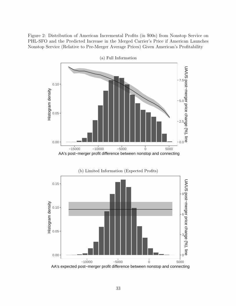
Figure 2: Distribution of American Incremental Profits (in $00s) from Nonstop Service onPHL-SFO and the Predicted Increase in the Merged Carrier’s Price if American LaunchesNonstop Service (Relative to Pre-Merger Average Prices) Given American’s Profitability

(a) Full Information

0.00

0.05

0.10

0.0

2.5

5.0

7.5

−15000 −10000 −5000 0 5000AA's post−merger profit difference between nonstop and connecting

His

togr

am d

ensi

tyU

A/U

S post−

merger price change (%

), line

(b) Limited Information (Expected Profits)

0.00

0.05

0.10

0.15

0

3

6

9

−10000 −5000 0 5000AA's expected post−merger profit difference between nonstop and connecting

His

togr

am d

ensi

tyU

A/U

S post−

merger price change (%

), line

33

Tab

le10

:P

redic

ted

Pri

cean

dSer

vic

eC

han

ges

for

Subse

quen

tC

omple

ted

Mer

gers

onR

oute

sw

her

eM

ergi

ng

Par

ties

are

Non

stop

Duop

olis

ts(B

asel

ine

Ass

um

pti

on)

Ave

rage

for

Del

ta/N

orth

wes

tU

nit

ed/C

onti

nen

tal

Am

eric

an/U

SA

irw

ays

Com

ple

ted

Mer

gers

Exp

.N

um

b.

Exp

.N

um

b.

Exp

.N

um

b.

Exp

.N

um

b.

Pri

ceN

ewN

onst

opP

rice

New

Non

stop

Pri

ceN

ewN

onst

opP

rice

New

Non

stop

Pre

-mer

ger

$566.3

9-

$503

.75

-$4

59.1

3-

$482

.25

-

Post

-Mer

ger

Ser

vic

eT

yp

esF

ixed

$593.2

0-

$556

.17

-$5

21.1

5-

$537

.86

-Allow

RivalServ

iceChanges

ConnectingRivals

NonstopQuality

andCostsDrawnfrom:

Con

dit

ion

al

Dis

trib

uti

ons

$59

0.3

40.

07$5

47.6

50.

14$5

11.3

30.

21$5

29.1

70.

18

Est

imat

edD

istr

ibu

tion

s$584

.20

0.19

$534

.08

0.35

$488

.45

0.73

$510

.45

0.57

Ave

rage

of

Mer

gin

gP

arti

es$5

73.

830.

93$4

54.3

62.

62$4

60.2

52.

10$4

72.2

32.

08

Nu

mb

erof

Rou

tes

24

1117

Tab

le11

:P

redic

ted

Pri

cean

dSer

vic

eC

han

ges

Wher

eM

ergi

ng

Par

ties

and

atL

east

One

Riv

alar

eN

onst

op

Del

ta/N

ort

hw

est

Un

ited

/Con

tin

enta

lA

mer

ican

/US

Air

way

sU

nit

ed/U

SA

irw

ays

Ave

rage

∆in

#O

f∆

in#

Of

∆in

#O

f∆

in#

Of

∆in

#O

fP

rice

NS

Riv

als

Pri

ceN

SR

ival

sP

rice

NS

Riv

als

Pri

ceN

SR

ival

sP

rice

NS

Riv

als

Pre

-mer

ger

$351.2

6-

$438

.08

-$3

63.1

1-

$350

.02

-$3

77.5

1-

Post

-Mer

ger

Ser

vic

eT

yp

esF

ixed

$382.0

4-

$464

.98

-$4

04.8

4-

$378

.15

-$4

12.2

7-

Allow

RivalServ

iceChanges

ConnectingRivals

NonstopQuality

andCostsDrawnfrom:

Con

dit

ion

alD

istr

ibu

tion

s$378

.90

0.16

$464

.86

0.01

$404

.41

0.03

$377

.24

0.05

$411

.07

0.06

Est

imat

edD

istr

ibu

tion

s$3

86.

40-0

.51

$466

.18

-0.0

3$4

03.5

5-0

.27

$375

.17

-0.1

1$4

13.3

3-0

.28

Ave

rage

of

Mer

gin

gP

arti

es$3

74.3

70.

66$4

55.6

40.

61$3

98.8

5-0

.03

$367

.68

0.48

$404

.95

0.34

Nu

mb

erof

Rou

tes

24

1010

26

Not

es:

see

not

esto

Tab

le9.

All

pre

dic

tion

sm

ake

the

bas

elin

em

erge

ras

sum

pti

onan

d,

wh

ense

rvic

ety

pes

are

end

ogen

ous,

use

1,00

0d

raw

sfr

omth

ere

leva

nt

dis

trib

uti

on.

Pre

-mer

ger

pri

ces

are

aver

ages

acro

ssth

em

ergi

ng

par

ties

.S

tan

dar

der

rors

not

rep

orte

d.

34

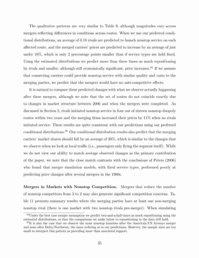
The qualitative patterns are very similar to Table 9, although magnitudes vary across

mergers reflecting differences in conditions across routes. When we use our preferred condi-

tional distributions, an average of 0.18 rivals are predicted to launch nonstop service on each

affected route, and the merged carriers’ prices are predicted to increase by an average of just

under 10%, which is only 2 percentage points smaller than if service types are held fixed.

Using the estimated distributions we predict more than three times as much repositioning

by rivals and smaller, although still economically significant, price increases.34 If we assume

that connecting carriers could provide nonstop service with similar quality and costs to the

merging parties, we predict that the mergers would have no anti-competitive effects.

It is natural to compare these predicted changes with what we observe actually happening

after these mergers, although we note that the set of routes do not coincide exactly due

to changes in market structure between 2006 and when the mergers were completed. As

discussed in Section 2, rivals initiated nonstop service in four out of sixteen nonstop duopoly

routes within two years and the merging firms increased their prices by 11% when no rivals

initiated service. These results are quite consistent with our predictions using our preferred

conditional distributions.35 Our conditional distribution results also predict that the merging

carriers’ market shares should fall by an average of 30%, which is similar to the changes that

we observe when we look at local traffic (i.e., passengers only flying the segment itself). While

we do not view our ability to match average observed changes as the primary contribution

of the paper, we note that the close match contrasts with the conclusions of Peters (2006)

who found that merger simulation models, with fixed service types, performed poorly at

predicting price changes after several mergers in the 1980s.

Mergers in Markets with Nonstop Competition. Mergers that reduce the number

of nonstop competitors from 3 to 2 may also generate significant competition concerns. Ta-

ble 11 presents summary results where the merging parties have at least one non-merging

nonstop rival (there is one market with two nonstop rivals pre-merger). When simulating

34Under the best case merger assumption we predict two-and-a-half times as much repositioning using theestimated distributions, so that the comparisons we make below to repositioning in the data still hold.

35It is also the case that we observe the most nonstop launches after the American/US Airways mergerand none after Delta/Northwest, the same ordering as in our predictions. However, the sample sizes are toosmall to interpret this pattern as providing more than anecdotal support.

35

counterfactuals, we assume that the merged firm will be nonstop and make the same as-

sumptions about connecting rivals that we have made previously. However, we also now

endogenize the service choice of the nonstop rival(s). For this carrier its nonstop quality

and marginal costs are observed, but we need to make assumptions about the quality and

marginal costs of its connecting service, and its fixed costs of providing nonstop service.36

When we use conditional distributions, we predict that the nonstop rival(s) will always

continue to provide nonstop service and that connecting carriers will rarely introduce nonstop

service. As a result, predicted price changes are almost identical to those where service types

are assumed fixed. This is consistent with our earlier results. However, differences emerge for

the other assumptions, because it becomes likely that the nonstop rival, which is usually a

quite effective nonstop competitor, may cease nonstop service and this type of repositioning

can lead to price increases. For example, a nonstop rival ceases nonstop service for around

one-third of simulations in the results reported in the bottom (“Average of Merging Parties”)

row of the table. As a result, we now predict significant price increases under all three

approaches, and the largest predicted prices increases and the greatest probability of post-

merger nonstop monopoly are when we use the estimated distributions. Therefore while the

intuition that the conditional distributions will tend to predict the largest prices increases

when nonstop duopolists merge is fairly clear, there are additional nuances for other market

structures that are relevant for merger analysis.

7 Conclusions

We have developed a model of endogenous service choices and price competition in airline

markets, assuming that carriers have full information about their demand and marginal costs

when they make their service choices. In this framework, carriers observed providing nonstop

or connecting service will be selected based on how competitive their nonstop service will be,

and this has implications for the likelihood and sufficiency of repositioning after horizontal

mergers. We believe the full information assumption is the natural one to use when predicting

36In the case where we assume that connecting rivals would have the same nonstop quality as the mergingparties, we use the observed nonstop quality and marginal costs for the nonstop rival(s), and draw its (their)connecting qualities and marginal costs, and fixed costs, from the estimated distributions.

36

product repositioning by experienced market participants, and when trying to test whether

repositioning will sustainably limit market power after a merger.

We have shown that the model can be estimated without an excessive computational

burden and that accounting for selection matters when performing merger simulations that

allow repositioning by rivals to occur. We believe that both findings are important for

academic research, while the second finding is the more directly relevant result for policy,

as the distributions of parameters used in a merger case are more likely to be drawn from

documents, expert testimony or simple calibrations, rather being estimated.37 Our approach

allows for a formal quantification of the likelihood and sufficiency concepts that are clear

in the Horizontal Merger Guidelines, but which are rarely analyzed in a systematic way,

even though the possibility that entry or repositioning may constrain market power has to

be addressed in almost all horizontal merger investigations conducted by the Department of

Justice, the Federal Trade Commission or their equivalents in other countries.

On nonstop duopoly routes we find that accounting for selection, by using conditional

distributions of unobservables that are consistent with pre-merger service choices, as well as

prices and market shares, predicts lower probabilities of repositioning by rivals, and larger

average price increases, than alternative approaches. These alternatives include either as-

suming that the nonstop service of rivals would be similar to that offered by the nonstop

incumbents before the merger, which might seem an appealing assumption in litigation, or

using new draws from estimated distributions, which has been done in the academic litera-

ture. Designing counterfactuals so that they would also predict observed pre-merger entry

or service choices is consistent with the logic of traditional merger simulations, and we find

that it also allows us to explain what is observed after actual mergers.

37For example, merging party data might be used to estimate distributions of marginal or fixed costswithout reference to a model. Experts often provide ranges of values for different types of cost, on top ofwhich the analyst might impose a reasonable distribution.

37

References

Ackerberg, D. (2009): “A New Use of Importance Sampling to Reduce ComputationalBurden in Simulation Estimation,” Quantitative Marketing and Economics, 7(4), 343–376.

Aguirregabiria, V., and C.-Y. Ho (2012): “A Dynamic Oligopoly Game of the USAirline Industry: Estimation and Policy Experiments,” Journal of Econometrics, 168(1),156–173.

Ashenfelter, O., D. Hosken, and M. Weinberg (2014): “Did Robert Bork Understatethe Competitive Impact of Mergers? Evidence from Consummated Mergers,” Journal ofLaw and Economics, 57(S3), S67–S100.

Baker, J. B. (1996): “The Problem with Baker Hughes and Syufy: On the Role of Entryin Merger Analysis,” Antitrust Law Journal, 65, 353–374.

Benkard, L., A. Bodoh-Creed, and J. Lazarev (2018): “Simulating the DynamicEffects of Horizontal Mergers: U.S. Airlines,” Discussion paper, Stanford University.

Berry, S. (1992): “Estimation of a Model of Entry in the Airline Industry,” Econometrica,60(4), 889–917.

Berry, S., and P. Jia (2010): “Tracing the Woes: An Empirical Analysis of the AirlineIndustry,” American Economic Journal: Microeconomics, 2(3), 1–43.

Borenstein, S. (1990): “Airline Mergers, Airport Dominance, and Market Power,” Amer-ican Economic Review, 80(2), 400–404.

(2010): “An Index of Inter-City Business Travel for Use in Domestic Airline Com-petition Analysis,” Discussion paper, UC Berkeley.

Carlton, D., M. Israel, I. MacSwain, and E. Orlov (2017): “Are Legacy AirlineMergers Pro-or Anti-Competitive? Evidence from Recent US Airline Mergers,” Interna-tional Journal of Industrial Organization.

Carlton, D. W. (2004): “Why Barriers to Entry are Barriers to Understanding,” AmericanEconomic Review, 94(2), 466–470.

Ciliberto, F., C. Murry, and E. T. Tamer (2018): “Market Structure and Competitionin Airline Markets,” Discussion paper, University of Virginia.

Ciliberto, F., and E. Tamer (2009): “Market Structure and Multiple Equilibria inAirline Markets,” Econometrica, 77(6), 1791–1828.

Ciliberto, F., and J. W. Williams (2014): “Does Multimarket Contact Facilitate TacitCollusion? Inference on Conduct Parameters in the Airline Industry,” RAND Journal ofEconomics, 45(4), 764–791.

Coate, M. B. (2008): “Theory Meets Practice: Barriers to Entry in Merger Analysis,”Review of Law & Economics, 4(1), 183–212.

38

Draganska, M., M. Mazzeo, and K. Seim (2009): “Beyond Plain Vanilla: ModelingJoint Product Assortment and Pricing Decisions,” Quantitative Marketing and Economics,7(2), 105–146.

Eizenberg, A. (2014): “Upstream Innovation and Product Variety in the US Home PCMarket,” Review of Economic Studies, 81(3), 1003–1045.

Fan, Y., and C. Yang (2018): “Competition, Product Proliferation and Welfare: A Studyof the US Smartphone Market,” Discussion paper, University of Michigan.

Fisher, F. M. (1987): “Horizontal Mergers: Triage and Treatment,” Journal of EconomicPerspectives, 1(2), 23–40.

Geweke, J. (1989): “Bayesian Inference in Econometric Models using Monte Carlo Inte-gration,” Econometrica, 57(6), 1317–1339.

Gillen, D., W. Morrison, and C. Stewart (2003): “Air Travel Demand Elasticities:Concept, Issues and Measurement,” Discussion paper, Canadian Department of Finance.

Huschelrath, K., and K. Muller (2014): “Airline Networks, Mergers, and ConsumerWelfare,” Journal of Transport Economics and Policy, 48(3), 385–407.

(2015): “Market Power, Efficiencies, and Entry: Evidence from an Airline Merger,”Managerial and Decision Economics, 36(4), 239–255.

Israel, M., B. Keating, D. L. Rubinfeld, and R. Willig (2013): “Airline NetworkEffects and Consumer Welfare,” Review of Network Economics, 12(3), 287–322.

Keyes, L. S. (1987): “The Regulation of Airline Mergers by the Department of Trans-portation,” Journal of Air Law & Commerce, 53, 737–764.

Kirkwood, J. B., and R. O. Zerbe (2009): “The Path to Profitability: Reinvigoratingthe Neglected Phase of Merger Analysis,” George Mason Law Review, 17, 39–112.

Koopman, S. J., N. Shephard, and D. Creal (2009): “Testing the Assumptions BehindImportance Sampling,” Journal of Econometrics, 149(1), 2–11.

Li, S., J. Mazur, Y. Park, J. Roberts, A. Sweeting, and J. Zhang (2018): “Repo-sitioning and Market Power After Airline Mergers,” Discussion paper, University of Mary-land.

Li, S., J. Mazur, J. Roberts, and A. Sweeting (2015): “Airline Mergers and thePotential Entry Defense,” Discussion paper, University of Maryland.

Li, T., and B. Zhang (2015): “Affiliation and Entry in First-Price Auctions with Hetero-geneous Bidders: an Analysis of Merger Effects,” American Economic Journal: Microeco-nomics, 7(2), 188–214.

Luttmann, A. (2019): “Evidence of Directional Price Discrimination in the US AirlineIndustry,” International Journal of Industrial Organization, 62, 291–329.

39

MacKay, A., and N. H. Miller (2018): “Instrument-Free Demand Estimation: Method-ology and an Application to Consumer Products,” Discussion paper, Georgetown Univer-sity.

Mizuno, T. (2003): “On the Existence of a Unique Price Equilibrium for Models of ProductDifferentiation,” International Journal of Industrial Organization, 21(6), 761–793.

Morrison, S. A. (1996): “Airline Mergers: A Longer View,” Journal of Transport Eco-nomics and Policy, 30(3), 237–250.

Nevo, A. (2000): “Mergers with Differentiated Products: The Case of the Ready-to-EatCereal Industry,” RAND Journal of Economics, 31(3), 39–421.

Park, Y. (2019): “The Welfare Implications of Slot Divestitures,” Discussion paper, Uni-versity of Maryland.

Peters, C. (2006): “Evaluating the Performance of Merger Simulation: Evidence from theU.S. Airline Industry,” Journal of Law and Economics, 49(2), 627–649.

Reiss, P. C., and P. T. Spiller (1989): “Competition and Entry in Small Airline Mar-kets,” Journal of Law and Economics, 32(2, Part 2), S179–S202.

Roberts, J. W., and A. Sweeting (2013): “When Should Sellers Use Auctions?,” Amer-ican Economic Review, 103(5), 1830–1861.

Schmalensee, R. (1987): “Horizontal Merger Policy: Problems and Changes,” Journal ofEconomic Perspectives, 1(2), 41–54.

Shapiro, C. (2010): “The 2010 Horizontal Merger Guidelines: From Hedgehog to Fox inForty Years,” Antitrust Law Journal, 77(1), 49–107.

Sweeting, A., J. W. Roberts, and C. Gedge (forthcoming): “A Model of DynamicLimit Pricing with an Application to the Airline Industry,” Journal of Political Economy.

Werden, G. J., A. S. Joskow, and R. L. Johnson (1991): “The Effects of Mergers onPrice and Output: Two Case Studies From the Airline Industry,” Managerial and DecisionEconomics, 12(5), 341–352.

Wollmann, T. (2018): “Trucks Without Bailouts: Equilibrium Product Characteristicsfor Commercial Vehicles,” American Economic Review, 108(6), 1364–1406.

40

APPENDICES TO “REPOSTIONING AND

MARKET POWER AFTER AIRLINE MERGERS”

FOR ONLINE PUBLICATION

A Example Comparing Services Choices Under Lim-

ited and Full Information Models

Our model and our counterfactuals assume that carriers have full information when making

service choices. We view full information as the most plausible description of the industry

and the appropriate way to analyze the medium-run effects of a merger. In Section 6 we

include one illustration of the effects of limited information, focusing on the profits and

competitiveness of a single carrier. In this Appendix we use an example to illustrate the

equilibrium effects of different information structures, which have not been clearly identified

in the existing literature. Our example is based on a slightly restricted version of the model

estimated in the paper (it assumes a single market per route, rather than allowing differences

in directional demands, and the marginal cost structure is simpler). It also uses one set of

parameter values, although the qualitative patterns are robust to many alternative values

that we have tried.

Overview. We consider a single market, although we shall vary its size, with six carriers,

A,..,F . In the first stage of the game, the carriers choose whether to provide connecting

service or higher-quality nonstop service. Nonstop service requires payment of a fixed cost.

Having selected their service types they simultaneously choose prices in the second stage.

Demand is determined by a nested logit model, with all carriers in the same nest. The quality

of a carrier’s service is determined by the sum of a fixed carrier-specific quality component,

which will always be known to rivals, a random component and, if it provides nonstop

service, a second random component which is truncated to be greater than zero. Marginal

costs consist of a common fixed service-specific component and a random component that

is common across service types. A carrier’s fixed cost is drawn from a normal distribution

41

with a common mean and variance. Service choices are made sequentially, where the carriers

with the highest fixed quality move first.

Parameters. The indirect utility for consumer k using carrier i is uki = βi−αpi+τζk+(1−

τ)εki, with τ = 0.7, α = 0.5, and βi = βCONi +βNSi x I(i is nonstop). βCONi is drawn from a

normal distribution with standard deviation 0.2 and mean values of 0.6, 0.55, 0.5, 0.45, 0.4

and 0.35 for carriers A to F respectively. The incremental quality of nonstop service, βNSi ,

is a draw from a truncated normal distribution with mean 0.3, standard deviation 0.2 and a

lower truncation point of 0. The mean utility of not traveling is zero. Carrier marginal costs

are $200 for nonstop service and $220 for (longer) connecting service, plus a carrier-specific

component, common across service types, drawn from a normal distribution with mean zero

and standard deviation $15. Nonstop service requires a carrier to pay a fixed cost that has

mean $600,000 and standard deviation $125,000.

Information Structures. We compare outcomes under two information structures. Un-

der full information, all draws are known to all carriers throughout the game. Under limited

information, carriers only know the model parameters and the draws of fixed costs (assumed

to be known by all carriers) in the first stage, but the demand and marginal cost draws are

revealed before prices are chosen. Limited information is the common assumption in the

empirical literature on models with entry or product selection and price competition (Dra-

ganska, Mazzeo, and Seim (2009), Eizenberg (2014), Wollmann (2018) and Fan and Yang

(2018)). We simulate equilibrium outcomes 50,000 times for each of 30 different market sizes,

ranging from 5,000 and 295,000.

The method for solving the full information model is the same as the one used in the

paper. For the limited information model, we approximate the expected profits of each carrier

in every possible market configuration by taking 1,000 draws of marginal costs and qualities.

We then solve sequential service choice games for each of 50,000 draws of fixed costs, before

simulating realizations of the marginal cost and quality draws to compute expected consumer

surplus.

42

Figure A.1: The Relationship Between Market Size, Expected Consumer Surplus and theExpected Number of Nonstop Carriers Under Different Informational Assumptions

0 0.5 1 1.5 2 2.5 3

Market Size 105

0

1

2

3

4

5

6

Num

ber

of N

onst

op C

arrie

rs

Expected Number of Nonstop Carriers

0 0.5 1 1.5 2 2.5 3

Market Size 105

100

105

110

115

120

125

130

135

140

145

Con

sum

er S

urpl

us (

$/co

nsum

er)

Expected Consumer Surplus

Limited InformationFull Information

Results. Figure A.1 compares the average number of nonstop carriers and consumer sur-

plus in equilibrium. In a small market, nonstop service may only be profitable when a

carrier has unusually high nonstop quality or low marginal costs, unless its fixed cost is very

low. Knowledge of quality and marginal cost draws can therefore make it more likely that

a carrier will be nonstop. Fewer carriers provide nonstop service in larger markets under

full information. The intuition comes from the competitiveness of the nonstop rivals that a

carrier expects to face. Under full information, a nonstop rival will tend to be a stronger

competitor (because it has been selected based on its quality and cost), which lowers the

expected nonstop profitability of another carrier considering nonstop service. This reduces

the number of nonstop carriers in equilibrium. However, selection also means that nonstop

carriers tend to provide better quality products, which raises expected consumer surplus

under full information for a given number of nonstop carriers. The example also illustrates

the feature that carriers may frequently regret their choices under limited information: for

example, for a market size of 55,000, for 48% of the draws where a single carrier chooses to be

nonstop, that carrier would have increased its (ex-post) profits by only offering connecting

service.

Figure A.2 shows that, for a given market size, the distribution of the number of nonstop

43

Figure A.2: The Relationship Between Market Size and Equilibrium Market Structure UnderDifferent Informational Assumptions

0 0.5 1 1.5 2 2.5 3

Market Size 105

0

0.1

0.2

0.3

0.4

0.5

0.6

0.7

0.8

0.9

1

Pro

pn. o

f Sim

ulat

ions

Limited Information

0 0.5 1 1.5 2 2.5 3

Market Size 105

0

0.1

0.2

0.3

0.4

0.5

0.6

0.7

0.8

0.9

1

Pro

pn. o

f Sim

ulat

ions

Full Information

No NonstopOne NonstopTwo NonstopThree NonstopFour NonstopFive NonstopSix Nonstop

carriers is much tighter under limited information.38 This feature has implications for what

we would predict should happen after a merger if carriers can change their service choices.

To illustrate, we consider a market size of 85,000 and collect all sets of draws that result in

the two carriers with the highest mean quality components being nonstop duopolists, which

is the most common outcome under either information structure. Now suppose that these

carriers merge, eliminating the carrier with the smaller market share, and that the remaining

carriers can re-optimize their service choices in the same sequential order.39 Under limited

information, the probability that at least one rival carrier will introduce nonstop service after

the merger is 0.8, and the expected reduction in consumer surplus following the merger is just

under $0.3m.. Under full information, the probability that at least one rival will introduce

nonstop service after the merger is 31% lower (0.55) and the expected loss of consumer surplus

is almost $1.15 million.40 In the limited information case, the merger is also, on average,

38For example, for a market size of 145,000, 97% of simulated outcomes have either three or four nonstopcarriers, compared with 69% under full information.

39The reader might view it as unreasonable to use the limited information assumption in this case becausecarriers’ pre-merger experience on the route in question would inform them of their quality and costs, evenfor the type of service that they are not offering. We completely agree, which is one reason why we believea full information model is the natural model for merger counterfactuals.

40The loss in consumer surplus is greater under full information not only because there is less repositioningbut also because the pre-merger market shares of the nonstop carriers, whose merger we are considering,

44

unprofitable for the merging parties, while it is profitable under full information. Note that

if, in either version of the model, we had not accounted for selection (which we did by only

using draws in our counterfactuals that could generate the pre-merger market structure that

we are interested in), we could also get quite different post-merger predictions. In Section 6

of the paper, we show how accounting for selection affects merger counterfactuals using our

estimated full information model.

B Data Appendix

This Appendix complements the description of the data in Section 2 of the text.

B.1 Sample Construction and Variable Definitions

Selection of markets. We use 2,028 airport-pair markets linking the 79 U.S. airports (exclud-

ing airports in Alaska and Hawaii) with the most enplanements in Q2 2006. The markets

that are excluded meet one or more of the following criteria:

• airport-pairs that are less than 350 miles apart as ground transportation may be very

competitive on these routes;

• airport-pairs involving Dallas Love Field, which was subject to Wright Amendment

restrictions that severely limited nonstop flights;

• airport-pairs involving New York LaGuardia or Reagan National that would violate

the so-called perimeter restrictions that were in effect from these airports41;

• airport-pairs where more than one carrier that is included in our composite “Other

Legacy” or “Other LCC” (low-cost) carriers are nonstop, have more than 20% of non-

directional traffic or have more than 25% presence (defined in the text) at either of

tend to be higher because of selection.41To be precise, we exclude routes involving LaGuardia that are more than 1,500 miles (except Denver)

and routes involving Reagan National that are more than 1,250 miles.

45

the endpoint airports. Our rationale is that our assumption that the composite carrier

will act as a single player may be especially problematic in these situations42; and,

• airport-pairs where, based on our market size definition (explained below), the com-

bined market shares of the carriers are more than 85% or less than 4%.

Seasonality. The second quarter is the busiest quarter for airline travel, and one might

be concerned that seasonality affects our measures of passenger flows and service choices,

and therefore our estimates. We do not believe that this is a first-order concern for our

sample of relatively large markets. The website http://www.anna.aero (accessed May 29,

2018) provides a formula for measuring the seasonality of airport demand (SVID) which we

have calculated for all of the airports in our sample using monthly T100 data on originating

passengers.43 The website classifies seasonality as “excellent” if SVID is less than 2 or “good”

if the SVID is between 2 and 10, on the basis that seasonality is costly for an airline or an

airport because it requires changes in schedules. All of the airports in our sample are within

these ranges, with the highest (most seasonal) values for Seattle (2.4), New Orleans (2.8),

Palm Beach (5.2) and Southwest Florida (9.9). In contrast, a non-sample airport with very

seasonal demand, Gunnason-Crested Butte (GUC), has an SVID of 65. Applying SVID on

a route-level to quarterly traffic, only one sample route (Minneapolis to Southwest Florida)

has an SVID greater than 10 (19), and the 95th percentile is 3.12.

We reach a similar conclusion if we identify markets which a carrier serves nonstop in our

data and in the second quarter of 2005, but which they did not serve nonstop in either Q1

2005 or Q1 2006 (i.e., markets where a carrier’s nonstop service may be seasonal). We can

only identify two such carrier-markets in our sample (United for San Antonio-San Francisco

and Sun Country (part of Other Low Cost) for Indianapolis-Kansas City), out of 8,065

carrier-markets.

Definition of players, nonstop and connecting service. We are focused on the decision

of carriers to provide nonstop service on a route. Before defining any players or outcomes,

42An example of the type of route that is excluded is Atlanta-Denver where Airtran and Frontier, whichare included in our “Other LCC” category had hubs at the endpoints and both carriers served the routenonstop.

43The measure is calculated as

∑m=1,..,M=12

(100×Traffica,m

Traffica−100

)2

1000 .

46

we drop all passenger itineraries from DB1 that involve prices of less than $25 or more than

$2000 dollars44, open-jaw journeys or journeys involving more than one connection in either

direction. Our next step is to aggregate smaller players into composite “Other Legacy”

and “Other LCC” carriers, in addition to the “named” carriers (American, Continental,

Delta, Northwest, Southwest, United and US Airways) that we focus on. Our classification

of carriers as low-cost follows Berry and Jia (2010). Based on the number of passengers

carried, the largest Other Legacy carrier is Alaska Airlines, and the largest Other LCC

carriers are JetBlue and AirTran.

We define the set of players on a given route as those ticketing carriers who achieve at

least a 1% share of total travelers (regardless of their originating endpoint) and, based on

the assumption that DB1 is a 10% sample, carry at least 200 return passengers per quarter,

with a one-way passenger counted as one-half of a return passenger. We define a carrier as

providing nonstop service on a route if it, or its regional affiliates, are recorded in the T100

data as having at least 64 nonstop flights in each direction during the quarter and at least

50% of the DB1 passengers that it carries are recorded as not making connections (some of

these passengers may be traveling on flights that make a stop but do not require a change

of planes). Other players are defined as providing connecting service.

There is some arbitrariness in these thresholds. However, the 64 flight and 50% nonstop

thresholds for nonstop service have little effect because almost all nonstop carriers far ex-

ceed these thresholds. For example, Figure B.1 shows that the carriers we define as nonstop

typically carry only a small proportion of connecting passengers. For the same reason, we

also model nonstop carriers as only providing nonstop service even if some of their passen-

gers fly connecting, although we include the connecting passengers when calculating market

shares. On the other hand, our 1% share/200 passenger thresholds do affect the number of

connecting carriers. For example, if we instead require players to carry 300 return passengers

and have a 2% share, the average number of connecting carriers per market falls by almost

one-third as marginal carriers are excluded.

Market Size. Market size is used to define market shares and to calculate counterfactual

quantities and profits. Given the role of market size in the identification and estimation of

44These fare thresholds are halved for one-way trips.

47

Figure B.1: Proportion of DB1 Passengers Traveling with Connections, Based on the Typeof Service

0 0.2 0.4 0.6 0.8 1

Propn. of Connecting Passengers

0

100

200

300

400

500

600

700

800

900

Num

ber

of R

oute

-Car

rier

Obs

.

(i) Nonstop Carriers

0 0.2 0.4 0.6 0.8 1

Propn. of Connecting Passengers

0

1000

2000

3000

4000

5000

6000

Num

ber

of R

oute

-Car

rier

Obs

.

(ii) Connecting Carriers

demand and entry-type models, the ideal definition should imply that variation in shares

across markets, or across directions, should reflect changes in prices, carrier characteristics

and service types, and it should be a good predictor of the number of nonstop firms.

A standard approach in the literature is to use the geometric average of the endpoint

MSA populations (e.g., Berry and Jia (2010), Ciliberto and Williams (2014)). However, this

performs poorly for airport-pair routes (MSA demand may be split between several airports)

and it cannot allow for the possibility that originating demand is systematically different at

the endpoints.

We therefore consider an alternative definition based on the estimates of a generalized

gravity equation, used previously in Sweeting, Roberts, and Gedge (forthcoming). The

model specifies that the total number of second quarter passengers on a route varies with a

linear function of the log of the count of originating and arriving passengers at each of the

endpoint airports (measured for the second quarter of the previous year), log route distance

and interactions of these lagged passengers flow and distance variables. The corresponding

Poisson regression is estimated using data from 2005-2011, including year, origin and desti-

nation fixed effects and an interaction between the origin and destination fixed effects and

48

a dummy for long-distance routes, defined as those over 2,300 miles.45 With the estimates

in hand, we calculate the expected number of passengers for each directional market for

Q2 2006, based on lagged values of passenger flows in Q2 2005. Our market size measure

multiplies this prediction by 3.5.

Two comparisons suggest that our measure provides a superior measure of market size

to estimates based on average population. Given that prices and service in each direction

on a route tend to be similar we would expect the correlation in the combined market share

of all of the carriers to be quite high: using our measure the correlation is 0.86 and using

the geometric average population it is 0.56. Consistent with this difference, if one estimates

our model using population-based market size measures, there is much greater unobserved

heterogeneity in demand than there is in our estimates. CMT, who use a population-based

measure, also estimate much more demand heterogeneity than we do.

Table B.1 examines the ability of the different market size variables to predict the number

of nonstop carriers on a route using an ordered probit model. Examination of the reported

pseudo-R2s shows that our gravity measure has much stronger predictive power, and that

when we add population based variables to a specification with a flexible function of our

measure (i.e., going from column (2) to column (5)) the R2 increases by less than 1%.

However, because we recognize that our market size measure is still imperfect, we also allow

for an additional route level unobservable that is common to the demand of all carriers, but

is unobserved by the researcher.

Prices and Market Shares. As is well-known, airlines use revenue management strategies

that result in passengers on the same route paying quite different prices. Even if more de-

tailed data (e.g., on when tickets are purchased) was available, it would likely not be feasible

to model these type of strategies within the context of a combined service choice and pricing

game. We therefore use the average price as our price measure, but allow for prices and mar-

ket shares (defined as the number of originating passengers carried divided by market size)

to be different in each direction, so that we can capture differences in passenger preferences

45The individual coefficients are not especially informative because of the interactions, but combiningthem shows reasonable patterns. For example, the expected number of passengers declines in route dis-tance, increases with both lagged originating traffic at the origin airport, and lagged arriving traffic at thedestination.

49

Table B.1: Market Size Measures and the Number of Nonstop Car-riers

(1) (2) (3) (4) (5)

Our Market Size 3.230 11.05 11.04(/10,000) (0.110) (0.440) (0.482)Our Market Size2 -8.933 -8.780

(0.560) (0.587)Our Market Size3 2.283 2.230

(0.190) (0.196)Geom. Avg. Pop 2.476 10.48 2.125(/1 m.) (0.136) (0.823) (0.966)Geom. Avg. Pop2 -12.98 -4.835

(1.536) (1.757)Geom. Avg. Pop3 4.977 2.433

(0.773) (0.877)

Ordered Probit CutoffsCutoff 1 0.730 1.596 0.725 1.801 1.813

(0.0369) (0.0604) (0.0460) (0.113) (0.126)Cutoff 2 2.082 3.350 1.722 2.844 3.571

(0.0563) (0.0965) (0.0548) (0.120) (0.146)Cutoff 3 3.915 4.995 2.761 3.890 5.217

(0.128) (0.132) (0.0789) (0.133) (0.171)Cutoff 4 6.987 6.877 4.134 5.181 7.112

(0.431) (0.333) (0.232) (0.240) (0.351)

Observations 2,028 2,028 2,028 2,028 2,028Pseudo-R2 0.262 0.368 0.0770 0.109 0.371

Notes: coefficients from an ordered probit regression where the depen-dent variable is the number of nonstop carriers in the non-directionalmarket. “Our market size” measure is the average of our measure ofmarket size across directions. Standard errors in parentheses. Numberof observations is equal to the number of markets.

50

(possibly reflecting frequent-flyer program membership) across different airports.46

Explanatory Variables Reflecting Airline Networks. The legacy carriers in our data oper-

ate hub-and-spoke networks. On many medium-sized routes local demand could not generate

sufficient variable profits to cover the fixed costs of nonstop service, but nonstop service may

be profitable once the value of passengers who will use a nonstop flight as one segment on

a longer journey is taken into account. While our structural model captures price compe-

tition for passengers traveling only the route itself, we allow for traffic to other destination

to reduce the effective fixed cost of providing nonstop service by including three carrier-

specific variables in our specification of fixed costs. Two variables are indicators for the

principal domestic and international hubs of the non-composite carriers. We define do-

mestic hubs as airports where more than 10,000 of the carrier’s ticketed passengers made

domestic connections in DB1 in Q2 2005 (i.e., one year before our estimation sample). Note

that some airports, such as New York’s JFK airport for Delta, that are often classified as

hubs do not meet our definition because the number of passengers using them for domes-

tic connections is quite limited even though the carrier serves many destinations from the

airport. International hubs are airports that carriers use to serve a significant number of

non-Canadian/Mexican international destinations nonstop. Table B.2 shows the airports

counted as hubs for each named carrier.

We also include a continuous measure of the potential connecting traffic that will be

served if nonstop service is provided on routes involving a domestic hub. The construction

of this variable, as the prediction of a Heckman selection model, is detailed next.

B.2 An Ancillary Model of Connecting Traffic

As explained in Section 2, we want to allow for the amount of connecting traffic that a carrier

can carry when it serves a route nonstop to affect its decision to do so. Connecting traffic is

especially important in explaining why a large number of nonstop flights can be supported

at domestic hubs in smaller cities, such as Charlotte, NC (a US Airways hub) and Salt Lake

46Carriers may choose a similar set of ticket prices to use in each direction but revenue managementtechniques mean that average prices can be significantly different. Fares on contracts that carriers negotiatewith the federal government and large employers may also play a role, but there is no data available on howmany tickets are sold under these contracts.

51

Tab

leB

.2:

Dom

esti

can

dIn

tern

atio

nal

Hubs

for

Eac

hN

amed

Car

rier

Air

line

Dom

esti

cH

ub

Air

por

tsIn

tern

atio

nal

Hub

Air

por

tsA

mer

ican

Chic

ago

O’H

are,

Dal

las-

For

tW

orth

,St.

Lou

isC

hic

ago

O’H

are,

Dal

las-

For

tW

orth

,N

ewY

ork

JF

K,

Mia

mi,

Los

Ange

les

Con

tinen

tal

Cle

vela

nd,

Hou

ston

Inte

rcon

tinen

tal

Hou

ston

Inte

rcon

tinen

tal,

New

ark

Del

taA

tlan

ta,

Cin

cinnat

i,Sal

tL

ake

Cit

yA

tlan

ta,

New

Yor

kJF

K

Nor

thw

est

Det

roit

,M

emphis

,M

innea

pol

isD

etro

it,

Min

nea

pol

is

Unit

edC

hic

ago

O’H

are,

Den

ver,

Was

hin

gton

Dulles

Chic

ago

O’H

are,

San

Fra

nci

sco,

Was

hin

gton

Dulles

Sou

thw

est

Phoen

ix,

Las

Veg

as,

Chic

ago

Mid

way

,B

alti

mor

enon

e

US

Air

way

sC

har

lott

e,P

hilad

elphia

,P

itts

burg

hC

har

lott

e,P

hilad

elphia

52

City (Delta). While the development of a model where carriers choose their entire network

structure is well beyond the scope of the paper, we use a reduced-form model of network

flows that fits the data well47 and which gives us a prediction of how much connecting traffic

that a carrier can generate on a route where it does not currently provide nonstop service,

taking the service that it provides on other routes as given. We include this prediction in

our model of entry as a variable that can reduce the effective fixed cost of providing nonstop

service on the route.48

Model. We build our prediction of nonstop traffic on a particular segment up from a

multinomial logit model of the share of the connecting passengers going from a particular

origin to a particular destination (e.g., Raleigh (RDU) to San Francisco (SFO)) who will use

a particular carrier-hub combination to make the connection. Specifically,

sc,i,od =exp(Xc,i,odβ + ξc,i,od)

1 +∑

l

∑k exp(Xl,k,o,dβ + ξl,k,od)

(2)

where Xc,i,od is a vector of observed characteristics for the connection (c)-carrier (i)-origin

(o)- destination (d) combination and ξc,i,od is an unobserved characteristic. The Xs are

functions of variables that we are treating as exogenous such as airport presence, endpoint

populations and geography. The outside good is traveling using connecting service via an

airport that is not one of the domestic hubs that we identify.49 Assuming that we have

enough connecting passengers that the choice probabilities can be treated as equal to the

observed market shares, we could potentially estimate the parameters using the standard

estimating equation for aggregate data (Berry 1994):

log(sc,i,od)− log(s0,od) = Xc,i,odβ + ξc,i,od. (3)

47This is true even though we do not make use of additional information on connecting times at differentdomestic hubs which could potentially improve the within-sample fit of the model, as in Berry and Jia(2010). As well as wanting to avoid excessive complexity, we would face the problem that we would notobserve connection times for routes that do not currently have nonstop service on each segment, but whichcould for alternative service choices considered in our model.

48We also use the predicted value, not the actual value, on routes where we actually observe nonstopservice.

49For example, the outside good for Raleigh to San Francisco could involve traveling via Nashville on anycarrier (because Nashville is not a domestic hub) or on Delta via Dallas Fort Worth because, during ourdata, Dallas is not defined as a domestic hub for Delta even though it is for American.

53

However, estimating (3) would ignore the selection problem that arises from the fact

that some connections may only be available because the carrier will attract a large share of

connecting traffic. We therefore introduce an additional probit model, as part of a Heckman

selection model, to describe the probability that carrier i does serve the full ocd route,

Pr(i serves route ocd) = Φ (Wi,c,odγ) . (4)

Sample, Included Variables and Exclusion Restrictions. We estimate our model using

data from Q2 2005 (one year prior to the data used to estimate our main model) for the

top 100 US airports. We use DB1B passengers who (i) travel from their origin to their

destination making at least one stop in at least one direction (or their only direction if they

go one-way) and no more than one stop in either direction; and, (ii) have only one ticketing

carrier for their entire trip. For each direction of the trip, a passenger counts as one-half of a

passenger on an origin-connecting-destination pair route (so a passenger traveling RDU-ATL-

SFO-CVG-RDU counts as 12

on RDU-ATL-SFO and 12

on RDU-CVG-SFO). Having joined

the passenger data to the set of carrier-origin-destination-connecting airport combinations,

we then exclude origin-destination routes with less than 25 connecting passengers (adding

up across all connecting routes) or any origin-connection or connection-destination segment

that is less than 100 miles long.50 We also drop carrier-origin-destination-connecting airport

observations where the carrier (or one of its regional affiliates) is not, based on T100, pro-

viding nonstop service on the segments involved in the connection. This gives us a sample of

5,765 origin-destination pairs and 142,506 carrier-origin-destination-hub connecting airport

combinations, of which 47,996 are considered to be served in the data.

In Xc,i,od (share equation), we include variables designed to measure the attractiveness of

the carrier i and the particular ocd connecting route. Specifically, the included variables are

carrier i’s presence at the origin and its square, its presence at the destination and its square,

the interaction between carrier i’s origin and destination presence, the distance involved in

flying route ocd divided by the nonstop distance between the origin and destination (we call

50Note while we will only use routes of more than 350 miles in the estimation of our main model, we usea shorter cut-off here because we do not want to lose too many passengers who travel more than 350 mileson one segment but less than 350 miles on a second segment.

54

this the ‘relative distance’ of the connecting route), an indicator for whether route ocd is the

shortest route involving a hub, an indicator for whether ocd is the shortest route involving a

hub for carrier i and the interaction between these two indicator variables and the relative

distance.

The logic of our model allows us to define some identifying exclusion restrictions in the

form of variables that appear in W but not in X. For example, the size of the populations

in Raleigh, Atlanta and San Francisco will affect whether Delta offers service between RDU

and ATL and ATL and SFO, but it should not be directly relevant for the choice of whether

a traveler who is going from RDU to SFO connects via Atlanta (or a smaller city such

as Charlotte), so these population terms can appear in the selection equation for whether

nonstop service is offered but not the connecting share equation. In Wc,i,od we include

origin, destination and connecting airport presence for carrier i; the interactions of origin

and connecting airport presence and of destination and connecting airport presence; origin,

destination and connecting city populations; the interactions of origin and connecting city

populations and of destination and connecting city populations, a count of the number of

airports in the origin, destination and connecting cities51; indicators for whether either of

the origin or destination airports is an airport with limitations on how far planes can fly

(LaGuardia and Reagan National) and the interactions of these variables with the distance

between the origin or destination (as appropriate) and the connecting airport; indicators for

whether the origin or destination airport are slot-constrained. In both Xi,c,od and Wi,c,od we

also include origin, destination and carrier-connecting airport dummies.

Results. We estimate the equations using a one-step Maximum Likelihood procedure

where we allow for residuals in (3) and (4), which are assumed to be normally distributed,

to be correlated. However, our predictions are almost identical using a two-step procedure

(the correlation in predictions greater than 0.999). The coefficient estimates are in Table

B.3, although the many interactions mean that it is not straightforward to interpret the

coefficients.

To generate a prediction of the connecting traffic that a carrier will serve if it operates

51For example, the number is 3 for the airports BWI, DCA and IAD in the Washington DC-Baltimoremetro area.

55

Table B.3: Estimation Coefficients for Ancillary Model of Connecting Traffic

Connecting Share Serve Route 12log 1+ρ

1−ρ log(std. deviation)

Constant 4.200 -8.712 -0.109 0.308(0.338) (0.823) (0.0860) (0.0150)

Presence at Origin Airport 4.135 6.052(0.396) (1.136)

Presence at Connecting Airport 11.90(0.721)

Presence at Destination Airport 2.587 6.094(0.396) (1.126)

Origin Presence X Connecting Presence -5.536(1.311)

Destin. Presence X Connecting Presence -5.771(1.303)

Population of Connecting Airport -1.20e-07(3.16e-08)

Origin Population X Origin Presence -5.09e-08(2.23e-08)

Destin. Population X Destination Presence -4.46e-08(2.35e-08)

Number of Airports Served from Origin 0.543(0.101)

Number of Airports Served from Destination 0.529(0.0984)

Origin is Restricted Perimeter Airport 0.0317(0.321)

Destination is Restricted Perimeter Airport -0.0865(0.305)

Origin is Slot Controlled Airport -1.098(0.321)

Destination is Slot Controlled Airport -1.055(0.331)

Distance: Origin to Connection -0.00146(0.000128)

Distance: Connection to Destination -0.00143(0.000125)

Origin Restricted X Distance Origin - Connection 0.000569(0.000207)

Destin. Restricted X Distance Connection - Destin 0.000602(0.000211)

Relative Distance -4.657(0.441)

Most Convenient Own Hub -0.357(0.192)

Most Convenient Hub of Any Carrier -0.574(0.442)

Origin Presence2 -2.797(0.429)

Destination Presence2 -1.862(0.449)

Relative Distance2 0.745(0.129)

Most Convenient Own Hub X Relative Distance2 0.479(0.151)

Most Convenient Hub of Any Carrier X 0.590Relative Distance (0.434)Origin Presence X Destination Presence -5.278

(0.513)

Observations 142,506 - - -

Notes: robust standard errors in parentheses.

56

nonstop on particular segment, we proceed as follows. First, holding service on other routes

and by other carriers fixed, we use the estimates to calculate a predicted value for each

carrier’s share of traffic on a particular ocd route. Second, we multiply this share prediction

by the number of connecting travelers on the od route to get a predicted number of passengers.

Third, we add up across all oc and cd pairs involving a segment to get our prediction of the

number of connecting passengers served if nonstop service is provided. There will obviously

be error in this prediction resulting from our failure to account for how the total number of

connecting passengers may be affected by service changes and the fact that service decisions

will really be made simultaneously across an airline network.

However we find that the estimated model provides quite accurate predictions of how

many connecting travelers use different segments, which makes us believe that it should be

useful when thinking about the gain to adding some marginal nonstop routes to a network.

For the named legacy carriers in our primary model, there is a correlation of 0.96 between

the predicted and observed numbers of connecting passengers on segments that are served

nonstop. The model also captures some natural geographic variation. For example, for

many destinations a connection via Dallas is likely to be more attractive for a passenger

originating in Raleigh-Durham (RDU) than a passenger originating in Boston (BOS), while

the opposite may hold for Chicago. Our model predicts that American, with hubs in both

Dallas (DFW) and Chicago (ORD), should serve 2,247 connecting DB1 passengers on RDU-

DFW, 1,213 on RDU-ORD and 376 on RDU-STL (St Louis), which compares with observed

numbers of 2,533, 1,197 and 376. On the other hand, from Boston the model predicts that

American will serve more connecting traffic via ORD (2,265, observed 2,765) than DFW

(2,040, observed 2,364).

B.3 Explanatory Power of Observed Variables for Service and En-

try Choices

We now present some descriptive regressions that illustrate two features of our data that are

significant for our analysis. First, observed covariates explain much of the variation in service

choice decisions in the data. As well as being an indication that our covariates are useful, we

57

are able to show that market and carrier-specific covariates can classify the vast majority of

the market-carrier observations as being either very likely or very unlikely to provide nonstop

service. This helps to explain why the estimates of our structural model imply that, if we

consider simultaneous service choices, there is usually a dominant service choice for almost

all carriers in most markets, implying that there should be a single equilibrium. It also

provides the intuition for identification: we observe many carriers whose choices are close

to being predetermined by the observables, so that service choices will not be correlated

with the quality and cost unobservables for the type of service that they offer. In this case,

conventional arguments for the identification of the demand and marginal cost equations

apply. Second, observed covariates have much less explanatory power for decisions to serve

the market at all, with either connecting or nonstop service, which is the decision modeled in

Berry (1992), Ciliberto and Tamer (2009) and Ciliberto, Murry, and Tamer (2018) (CMT).

This may helps to explain why these papers find that their estimates imply that multiple

equilibria usually exist, whereas ours do not.

Table B.4 shows estimates from several probit specifications. In the first four columns

the dependent variable is equal to one if the carrier is nonstop, and we use the 8,065 carrier-

market observations in our data. The regressors in column (1) are observed market character-

istics, including the average of our market size measure across directions, and the observable

carrier variables that we include in our specification of fixed costs, including our measure of

connecting traffic that will be generated if the route is served nonstop. Despite the simplicity

of the specification the pseudo-R2 is 0.52. Column (2) replaces our market size measure with

the geometric average population measure that is most commonly used in the literature: the

pseudo-R2 decreases to 0.45, indicating that this is a poor alternative to our market size

measure (a result which is consistent with the results presented in Table B.1). Column (3)

adds measures of the carrier’s presence at each endpoint, which we allow to affect demand,

to the first specification, and the pseudo-R2 increases to 0.65.

Based on these estimates, Figure B.2(a), shows the distribution of predicted probabilities

for a carrier providing nonstop service using 40 bins based on column (3). We observe that

the predicted probabilities are concentrated either very close to zero or close to one. This

indicates that there are many carriers in our data for whom their unobservable quality and

58

Table B.4: Probit Models of Carrier Service Choice and Entry Decisions

(1) (2) (3) (4) (5)Dep. Var. Nonstop Nonstop Nonstop Nonstop Enter

Low Cost Carrier 0.808 0.782 0.537 1.681 0.514(0.0516) (0.0476) (0.0685) (0.395) (0.0376)

Slot Constr. Airport 0.587 0.724 0.541 0.232 -0.207(0.0961) (0.0927) (0.112) (0.132) (0.0650)

Carrier Intl. Hub 0.946 0.836 0.0385 -0.165 0.158(0.0748) (0.0738) (0.0894) (0.113) (0.0801)

Carrier Dom. Hub -6.161 -6.942 -6.578 -34.24 -3.740(0.647) (0.623) (0.648) (47.37) (0.627)

Carrier Pred. Connecting 1.355 1.464 1.160 5.701 0.611Traffic Measure (0.107) (0.104) (0.108) (7.932) (0.106)

Route Business Index -0.663 -1.364 0.198 0.670 -0.126(0.293) (0.268) (0.348) (0.387) (0.142)

Our Market Size 1.595 2.019 -0.176 -0.0552/10,000 (0.0649) (0.0828) (0.671) (0.0405)

Geom. Avg. Pop. 0.0122/10,000 (0.00112)

Carrier Max. 3.543 4.334 1.622Endpoint Presence (0.144) (0.626) (0.109)

Carrier Min. 1.916 6.814 4.424Endpoint Presence (0.276) (2.510) (0.266)

Number Rival -0.167Carriers in Market (0.0237)

Number Rival Low Cost 0.167Carriers in Market (0.0663)

Constant -2.065 -1.581 -3.930 -4.131 -0.312(0.127) (0.115) (0.177) (0.387) (0.0662)

Variable interactions N N N Y N

Observations 8,065 8,065 8,065 8,065 12,550Pseudo-R2 0.522 0.450 0.653 0.726 0.134

Notes: standard errors in parentheses. Observations in columns (1)-(4) are thecarrier-market observations that are included in our estimation dataset. Our Mar-ket Size is the average of our market size estimate across directions. Geom. Avg.Pop. is the geometric average of the MSA endpoint populations, a popular alter-native measure of market size. We measure carrier presence (the number of routesserved nonstop by the carrier out of the total number of routes served nonstop byany carrier) at the carrier-airport level and include the higher and lower values sepa-rately in the regressions. Observations in column (5) include the observations in ourestimation dataset plus observations for carrier-markets where the carrier providessome service at both endpoints but does not meet our criteria for being a competi-tor on the route in question. The interactions that are included in column (5) arebetween LCC, domestic hub, the predicted connecting traffic, market size and thetwo presence measures.

59

Figure B.2: Predicted Probabilities of Carrier Service Choices (based on Table B.4, column(3)) and Entry Decisions (based on Table B.4, column (5))

0 0.1 0.2 0.3 0.4 0.5 0.6 0.7 0.8 0.9 1

Predicted Probability of Nonstop Service

0

1000

2000

3000

4000

5000

6000

Num

b. o

f Car

rier-

Mar

kets

(a) Predicted Probability of Nonstop Service

0.2 0.3 0.4 0.5 0.6 0.7 0.8 0.9 1

Predicted Probability of Entry

0

200

400

600

800

1000

Num

b. o

f Car

rier-

Mar

kets

(b) Predicted Probability of Entry

60

cost draws should be essentially unselected for the type of service that they offer, allowing

for conventional identification arguments to apply.

To have more than one equilibrium outcome in a simultaneous move service choice game it

must be the case that there are two or more carriers who do not have dominant service choice

strategies. We can get a sense of whether multiple equilibria are likely to be common by

counting the number of markets where two or more carriers have intermediate probabilities of

nonstop service based on their observables (of course, based on the realized unobserved draws

one or both of these carriers may also have dominant strategies). Defining intermediate as

predicted probabilities between 0.05 and 0.95 based on the column (3) estimates, there are

482 markets (less than 24%) where two or more carriers have intermediate nonstop service

probabilities (using thresholds of 0.1 and 0.9, 302 markets would have at least two carriers

with intermediate probabilities).

In column (4) we include interactions between a number of the variables in the specifi-

cation (as noted beneath the table) as well as measures of the number of rival carriers, and

we find the pseudo-R2 increases to 0.72.

In column (5) we consider instead the decision to enter a market (i.e., to provide either

type of service) among the carriers that provide service (to any destinations) at both airport

endpoints and use a specification similar to column (3). This is the type of binary choice

modeled in in Berry (1992), Ciliberto and Tamer (2009) and CMT. Observed covariates

have much less explanatory power for this decision, and, as shown in Figure B.2(b), the

predicted probabilities for most carrier-markets lie in the range from 0.2 to 0.8. If we again

define intermediate probabilities as those between 0.05 and 0.95 based on the column (5)

estimates, 96% of markets have two or more carriers with intermediate entry probabilities.

This helps to explain why multiple equilibria are very common in their estimated models,

while being rare in ours.

61

B.4 An Analysis of Changes to Prices and Service After Airline

Mergers Post-2006

We use our model to predict the effects of three legacy carrier mergers that took place after

the period of our data (Delta/Northwest merger (closed October 2008), United/Continental

(October 2010) and American/US Airways (December 2013)). In this Appendix we describe

an analysis of what happened to the prices and quantities of the merging parties and the

service decisions of rivals on routes where the merging parties were nonstop duopolists. Based

on a fixed service types, one would expect that the merger might create significant market

power in these markets. We also consider the Southwest/Airtran merger (May 2011) although

we do not perform counterfactuals for that merger as Airtran is part of our composite Other

LCC carrier. To perform the analysis, we created a panel dataset that runs from the first

quarter of 2001 to the first quarter of 2017 using the same definition of nonstop service, but

without aggregating smaller carriers into composite Other Legacy and Other LCC rivals.

B.4.1 Frequency of Rivals Launching Nonstop Service

On routes where the merging firms are nonstop duopolists before the merger, the merged

firm always maintains nonstop service until the end of our data. We calculate the number of

routes where at least one rival carrier, including carriers that were not providing any service

prior to the merger, initiated nonstop service within two (three) years of the merger closing.

A two year window is often considered when examining entry and repositioning in merger

cases, and was explicitly cited by the Department of Transportation (Keyes (1987)). We will

use three years in our analysis of price and quantity changes below as an additional year

provides more precision to our estimates which are based on a small number of markets,

with little effect on the point estimates.

We find that no rivals (no rivals) initiated nonstop service on five routes where the

merging parties were nonstop duopolists immediately before the closing of the merger for

Delta/Northwest. Rivals did initiate nonstop service on one (two) out of five routes for

United/Continental, three (four) out of six routes for American/US Airways and one (one)

out of seventeen nonstop duopoly routes for Southwest/Airtran. Therefore, the overall rate

62

of rivals initiating nonstop service was five (seven) out of thirty-three routes, or four (six)

out of sixteen if we only consider legacy mergers.52

One explanation for a low rate of repositioning is that rivals are ill-suited to provide

nonstop service on these routes, so that the merging carriers can exercise market power even

if the merger does not generate efficiency advantages (higher quality or lower marginal costs).

This will be the explanation that we focus on in our counterfactuals. However, an alternative

explanation is that it is efficiencies created through the merger make it unattractive for rivals

to offer nonstop service. An analysis of changes to price and market shares can give some

insights into which of these stores are correct.

B.4.2 Changes to the Merging Carriers’ Prices and Quantities

We define a treatment group of markets where the merging carriers were nonstop duopolists

prior to the merger. We also define a control group of markets where one of the merging

carriers is nonstop and the other is either not in the market at all or is at most a quite

marginal connecting carrier, with a nondirectional share of traffic of less than 2%. How-

ever, we acknowledge that the literature has defined control groups in a number of different

ways, with different results (see the literature review in the Introduction), and that to the

extent that carriers offer networks, it is implausible that the control markets would be com-

pletely unaffected by changes in the treatment markets. We also restrict the control group

to only include routes where no carriers initiated new nonstop service after the merger. We

define three year pre- and post-merger windows (this provides more power than two year

windows, although the pattern of the coefficients are similar using two or three year win-

dows). For Delta/Northwest the windows are Q3 2005-Q2 2008 and Q1 2009-Q4 2011. For

United/Continental the windows are Q3 2007-Q2 2010 and Q1 2011-Q4 2013. For American-

US Airways the situation is less straightforward as detailed negotiations between the parties,

a bankruptcy judge and the Department of Justice were known to be ongoing from at least

August 2012. We therefore use windows of Q3 2009-Q2 2012 and Q2 2014-Q1 2017.53 For

Southwest/Airtran we use windows of Q2 2007-Q1 2010 and Q3 2010-Q2 2013.

52There is no overlap in the routes across these mergers.53We exclude two American/US Airways markets where rivals began service between the end of the pre-

merger window and the financial closing of the merger from the treatment group.

63

We use a regression specification

yimt = β0 + β1 ∗ Treatmentim ∗ Post-Mergerit +Ximtβ2 +Qtβ3 +Mimβ4 + εimt

where yimt is the outcome variable (the log of the weighted average price or the log of

the combined number of local passengers (i.e., passengers just flying the route itself and

not making connections to other destinations) on the merging carriers) for merging carrier

i in directional airport-pair market m in quarter t, Qt and Mim are quarter and carrier-

market dummies and β1 is the coefficient of interest.54 m is defined directionally, but we

cluster standard errors on the non-directional route. Ximt contains dummy controls for the

number of competitors (including connecting carriers), distinguishing between legacy and

LCC competitors, and one-quarter lagged fuel prices interacted with route nonstop distance

and its square. A route is defined to be in the treatment or the control group based on the

observed market structure in the last four quarters of the pre-merger window (so to be in

the treatment group, for example, both merging carriers must be nonstop in each of these

quarters). Note that this means that the treatment samples are different and smaller than

those considered for the repositioning analysis above, where we defined duopoly based on

the one quarter immediately before the financial closing of the merger. They can also differ

from the routes used in our counterfactuals where we will use the market structure from Q2

2006.

The results are presented in Table B.5. We report results for each merger and for the

three legacy mergers combined. The upper part of the table presents the results when we

only include treatment markets where there is no rival nonstop entry before or during the

post-merger window. In the lower panel we only use treatment markets where at least

one rival initiated nonstop service after the financial closure of the merger but before or

during the post-period window, and, for these markets, we only include post-merger window

observations where this rival service was actually provided.

The results are suggestive, despite the small number of treatment observations. For the

legacy mergers the pattern is that prices increase and the number of local passengers falls in

54To be clear, in the pre-merger period we combine the number of passengers on the merging carriers anduse their weighted average fare, so there is a single observation per market-quarter.

64

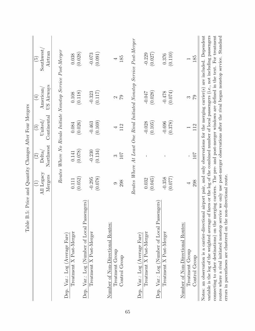
Tab

leB

.5:

Pri

cean

dQ

uan

tity

Chan

ges

Aft

erF

our

Mer

gers

(1)

(2)

(3)

(4)

(5)

All

Leg

acy

Del

ta/

Unit

ed/

Am

eric

an/

Sou

thw

est/

Mer

gers

Nor

thw

est

Con

tinen

tal

US

Air

way

sA

irtr

an

Rou

tes

Whe

reN

oR

ival

sIn

itia

teN

onst

opS

ervi

ceP

ost-

Mer

ger

Dep

.V

ar.:

Log

(Ave

rage

Far

e)

Tre

atm

ent

XP

ost-

Mer

ger

0.11

10.

141

0.08

40.

108

0.03

8(0

.052

)(0

.078

)(0

.026

)(0

.118

)(0

.028

)D

ep.

Var

.:L

og(N

um

ber

ofL

oca

lP

asse

nge

rs)

Tre

atm

ent

XP

ost-

Mer

ger

-0.2

95-0

.230

-0.4

63-0

.323

-0.0

73(0

.078

)(0

.134

)(0

.169

)(0

.117

)(0

.091

)

Num

ber

ofN

on-D

irec

tion

alR

oute

s:T

reat

men

tG

roup

93

42

4C

ontr

olG

roup

298

107

112

7918

5

Rou

tes

Whe

reA

tL

east

On

eR

ival

Init

iate

dN

onst

opS

ervi

ceP

ost-

Mer

ger

Dep

.V

ar.:

Log

(Ave

rage

Far

e)

Tre

atm

ent

XP

ost-

Mer

ger

0.03

2-

-0.0

28-0

.047

-0.2

29(0

.045

)(0

.105

)(0

.028

)(0

.027

)D

ep.

Var

.:L

og(N

um

ber

ofL

oca

lP

asse

nge

rs)

Tre

atm

ent

XP

ost-

Mer

ger

-0.3

58-

-0.6

96-0

.478

0.37

6(0

.077

)(0

.378

)(0

.074

)(0

.110

)

Num

ber

ofN

on-D

irec

tion

alR

oute

s:T

reat

men

tG

roup

4-

13

1C

ontr

olG

roup

298

107

112

7918

5

Not

es:

an

obse

rvati

on

isa

carr

ier-

dir

ecti

on

alai

rpor

tp

air,

and

only

obse

rvat

ion

sfo

rth

em

ergi

ng

carr

ier(

s)ar

ein

clud

ed.

Dep

end

ent

vari

able

isth

elo

gof

the

wei

ghte

dav

erage

offa

res

orth

elo

gof

the

com

bin

ednu

mb

erof

loca

lp

asse

nge

rs(i

.e.,

not

incl

ud

ing

pas

sen

gers

con

nec

tin

gto

oth

erd

esti

nat

ion

s)on

the

mer

gin

gca

rrie

rs.

Th

ep

re-

and

pos

t-m

erge

rw

ind

ows

are

defi

ned

inth

ete

xt.

For

trea

tmen

tro

ute

sw

her

ea

riva

lin

itia

ted

non

stop

serv

ice

we

only

use

pos

t-m

erge

rob

serv

atio

ns

afte

rth

eri

val

beg

ann

onst

opse

rvic

e.S

tan

dar

der

rors

inp

are

nth

eses

are

clu

ster

edon

the

non

-dir

ecti

onal

rou

te.

65

the treatment markets when no rivals initiate nonstop service, consistent with an increase

in market power and limited synergies from combining service on the treatment routes. The

fall in the number of local passengers is large, but this pattern appears to be robust: for

example, if we also include a linear time trend for the treatment group markets, to allow for

the possibililty that demand was falling in the type of markets that are nonstop duopolies,

the coefficient is -0.293 with a standard error of 0.092. This is almost identical to the

coefficient of -0.295 reported in Table B.5, column (1). On the other hand, in markets where

rival nonstop service is initiated there is no clear pattern of price increases. The number of

passengers declines in these markets, presumably due to competition from the new nonstop

carrier.

The pattern is different for Southwest/Airtran, although we note that we have fewer

treatment routes than the sixteen routes that were nonstop duopolies immediately before

the merger because, in a number of markets, a legacy carrier stopped its nonstop service

during the pre-merger window once both Southwest and Airtran were nonstop. There is no

statistically significant price increase on the nonstop duopoly routes when Southwest and

Airtran merge and there is no statistically significant decline in the number of passengers.

This result suggests that this LCC merger may have generated route-level synergies.

66

C Estimation

This Appendix provides additional detail on both the estimation process and our estimates.

Appendix C.1 explains how we solve the model. Appendix C.2 lays out the details for

our baseline specification where we assume that carriers make service choices in a known

order. Appendices C.3-C.6 analyze aspects of the performance of the estimation algorithm

in more detail, including the fit of the model and the robustness of the results to reducing the

number of moments. Appendix C.7 presents estimation results using moment inequalities.

The reader is referred to Li, Mazur, Park, Roberts, Sweeting, and Zhang (2018) for details of

a Monte Carlo procedure that illustrates the good performance of our estimation procedures,

under our baseline assumption and using inequalities.

C.1 Solving the Model

Our baseline assumption is that service choices are made sequentially in a known order. For

a given set of service choices on a given route, we can solve for a unique Bertrand Nash

pricing in each direction by solving the system of first-order conditions. One approach for

solving the service choice game would be to compute equilibrium variable profits for each

possible service choice combination and then apply backwards induction. However, we are

able to speed up solving the game, by 80% or more, by selectively growing the game tree

forward.

To do so, we first calculate whether the first mover would earn positive profits as a nonstop

carrier if it were the only carrier in the market, given its fixed cost.55 If not, then we do

not need to consider any of the branches where it provides nonstop service, immediately

eliminating half of the game tree from consideration. If it is profitable, then we need to

consider both branches. We then turn to the second carrier, and ask the same question,

for each of the first carrier branches that remain under consideration, and we only keep the

nonstop branch for the second carrier if nonstop service yields it (i.e., the second carrier)

positive profits. Once this has been done for all carriers, we can solve backwards to find the

55To be clear, this is not the same as testing whether nonstop service is more profitable than connectingservice.

67

unique subgame perfect equilibrium using the resulting tree, which usually has many fewer

branches than the full game tree.

C.2 Moments, Supports and Starting Values

Estimation involves a two-step procedure, where the first step involves solving a large number

of simulated games and the second step estimates the structural parameters by minimizing

a simulated method of moments objective function. We describe the procedure for our

preferred specification, with a sequential order of moves in the service choice game.

The second step objective function is

m(Γ)′Wm(Γ)

where W is a weighting matrix. m(Γ) is a vector of moments where each element has the

form 12,028

∑m=2,028m=1

(ydatam − Em(y|Γ)

)Zm, where subscript ms represent markets. ydatam are

observed outcomes and Zm are a set of observed exogenous variables that serve as instru-

ments.

Importance Draws. As described in the main text, Em(y|Γ) is approximated using im-

portance sampling. In the first step of the estimation procedure, we solve for the unique

equilibrium outcomes for S sets of the demand and cost draws θms, drawn from importance

densities g(θ|Xm). When estimating the parameters in the second step, we calculate

Em(y|Γ) =1

S

S∑s=1

y(θms, Xm)f(θms|Xm,Γ)

g(θms|Xm).

To apply this approach, we need to specify, before estimation, the support of each of the

θ draws and to choose the importance density g. Table C.1 lists the specifications used for

our reported estimates. The supports are chosen to contain all values that were likely to

be relevant, although we limit the support of the nesting parameter after finding that the

objective function had local minima with implausibly high or low mean values of τ when we

68

Table C.1: Description of g For the Final Round of Estimation

Market Draw Symbol Support gMarket Random Effect vm [-2,2] N(0, 0.4112)Market Nesting Parameter τm [0.5,0.9] N(0.634, 0.0282)Market Demand Slope αm [-0.75,-0.15] N(Xα

mβα, 0.0222)(price in $00s)

Carrier Draw

Carrier Connecting Quality βCON,A→Bim [-2,10] N(XCONim βCON , 0.2192)

Carrier Incremental Nonstop Quality βNSim [0,5] N(XNSim βNS, 0.2572)

Carrier Marginal Cost ($00s) cim [0,6] N(XMCim βMC , 0.1732)

Carrier Fixed Cost ($m) Fim [0,5] N(XFimβF , 0.2342)

Notes: where the covariates in the Xs are the same as those in the estimated model, andthe values of the βs for the final (initial) round of draws are as follows: βα.constant=−0.668 (−0.700), βα.bizindex=0.493 (0.600), βα.tourist= 0.097 (0.2), βCON .legacy= 0.432(0.400), βCON .LCC= 0.296 (0.300), βCON .presence= 0.570 (0.560), βNS .constant= 0.374(0.500), βMC .legacy= 1.802 (1.600), βMC .LCC= 1.408 (1.400), βMC .nonstop distance=0.533 (0.600), βMC .nonstop distance2 = −0.005 (-0.01), βMC .conn distance= 0.597 (0.700),βMC .conn distance2 = −0.007 (-0.020), the remaining marginal cost interactions are set equal tozero, βF .constant= 0.902 (0.750), βF .dom hub= 0.169 (-0.25), βF .conn traffic= −0.764 (-0.01),βF .intl hub= −0.297 (-0.55), βF .slot constr= 0.556 (0.700). In the initial round the standard de-viations of the draws were as follows: random effect 0.5, nesting parameter 0.1, slope parameter0.1, connecting quality 0.2, nonstop quality premium 0.5, marginal cost 0.15, fixed cost 0.25.

used [0, 1].56 Draws from the gs are taken independently for each market, carrier and type

of draw, although the market random effect induces correlation in demand across carriers in

a given market.

To choose the mean and standard deviation parameters of the g densities, we initially

attempted to match (by eye) a small number of price, market share and entry moments to

make sure that our model could capture the main patterns in the data. This led to the

“initial” parameterization reported in the notes to the Table C.1, where we tried to allow

for sufficiently large standard deviations that, during estimation, there would be enough

draws covering a wide range of qualities and costs that the mean coefficients could move

significantly if this allowed the estimated model to achieve a better fit. We then ran a couple

of rounds of our estimation routine to identify the parameters that we use to create the

draws for the final round of estimation whose results we report. While the estimator can be

56The assumed range of τ is consistent with most values in the literature: for example, Berry and Jia(2010) and Ciliberto and Williams (2014) report estimates between 0.62 and 0.77.

69

consistent for any set of gs that give finite variances, Ackerberg (2009) recommends using a

multi-round estimation procedure to improve efficiency.57 We take 2,000 sets of draws from

the gs for each market. 1,000 sets are used in the estimation (i.e., S = 1, 000), with the full

sets of 2,000 being used as a pool of draws that we use when performing a non-parametric

bootstrap to calculate standard errors.

Moments. Table C.2 presents a cross-tab describing the moments (interactions between

outcomes and exogenous variables) that we use for our baseline estimates. There are two

types of outcomes: market-specific and carrier-specific, and for each of these types, we are in-

terested in prices, market shares and service choices. For example, market-specific outcomes

include weighted average connecting and nonstop prices in each direction. Carrier-specific

outcomes include the carrier’s price in each direction, its market share in each direction and

whether it provides nonstop service. The exogenous Z variables can be divided into three

groups: market-level variables, variables that are specific to a single carrier, and variables

that measure the characteristics of the other carriers that are in the market (e.g., Delta’s

presence at each of the endpoint airports when we are looking at an outcome that involves

United’s price or service choice).

The resulting number of moments (1,384) is large given that our sample consists of 2,028

markets and 16,130 carrier-market-directions. This creates two issues. The first is that we

cannot claim that estimates of the covariance of the moments will be accurate. We therefore

use a diagonal weighting matrix (W ) with equal weight on the price, share and service-type

moments, and, within each of these groups, the weight on a particular moment is based

on the reciprocal of the variance based on initial estimates (estimated using an identity

weighting matrix).58 Second, one might wonder whether the large number of moments could

lead to small sample bias. In Appendix C.6 we show that the coefficient estimates, fit and

57A formal iterated procedure was used by Roberts and Sweeting (2013) in estimating a model of selectiveentry for auctions, where the standard errors were bootstrapped to account for this multi-stage estimationprocedure. To implement this bootstrapping approach, to account for what happens in the early iterations,in the current setting would create a large computational burden, so we instead present our results as beingconditional on the final round g, while acknowledging that the choice of g was informed by our initial attemptsat estimation. See Li, Mazur, Park, Roberts, Sweeting, and Zhang (2018) for an illustration of how differentgs affect the estimates in a Monte Carlo.

58The sum of the values on the diagonal of the weighting matrix equals 1 for each of the three groups ofmoments.

70

Table C.2: Moments Used in Estimation

Market Specific (yM) Carrier Specific (yC)Endogenous Outcomes Endogenous Outcomes

Exogenous Variables (Z) 7 outcomes 5 per carrier Row TotalMarket-Level Variables 49 315 364(ZM) (7 per market)

Carrier-Specific Variables 280 200 480(ZC) (up to 5 per carrier)

“Other Carrier”-Specific 315 225 540Variables (Z−C)(5 per “other carrier”)

Column Total 644 740 1,384

Notes: ZM = {constant, market size, market (nonstop) distance, business index, number oflow-cost carriers, tourist dummy, slot constrained dummy}ZC = {presence at each endpoint airport, our measure of the carrier’s connecting traffic if theroute is served nonstop, connecting distance, international hub dummy} for named legacy carriersand for Southwest (except the international hub dummy). For the Other Legacy and Other LCCCarrier we use {presence at each endpoint airport, connecting distance} as we do not model theirconnecting traffic. Carrier-specific variables are interacted with all market-level outcomes andcarrier-specific outcomes for the same carrier.Z−C = {the average presence of other carriers at each endpoint airport, connecting passengers,connecting distance, and international hub dummy} for each other carrier (zero if that carrier isnot present at all in the market).yM = {market level nonstop price (both directions), connecting price (both directions), sum ofsquared market shares (both directions), and the square of number of nonstop carriers}.yC = {nonstop dummy, price (both directions), and market shares (both directions)} for eachcarrier.

71

counterfactual results are very similar using only the 740 carrier-specific moments.

C.3 Performance of the Estimation Algorithm For the Baseline

Estimates

The use of importance sampling during estimation has two benefits: it greatly reduces the

computational burden and it generates a smooth objective function. As noted in the text, the

first step of our estimation routine (solving 2,000 simulated games for each market) takes less

than two days on a small cluster, while estimation of the parameters takes around one day on

a desktop or laptop computer without any parallelization. Figure C.1 illustrates the second

property, showing the shape of the objective function when we vary each parameter around

its estimated value, holding the other parameters fixed. While these pictures certainly should

not be interpreted as strong evidence that there is a global minimum in multiple dimensions,

it is comforting that the objective function is convex in almost all dimensions.

C.4 Variance of the Moments

For an importance sample estimate of a moment to be consistent the variance of y(θms, Xm)f(θms|Xm,Γ)g(θms|Xm)

must be finite (Geweke (1989)). One informal way to assess this property in an application

(Koopman, Shephard, and Creal (2009)) is to plot how an estimate of the sample variance

changes with S, and, in particular, to see how ‘jumpy’ the variance plot is as S increases. The

intuition is that if the true variance is infinite, the estimated sample variance will continue

to jump wildly as S rises.

Figure C.2 shows these estimates of the sample variance for the moments associated with

three market-level outcomes, namely the weighted nonstop fare, the weighted connecting

fare and the quantity-based sum of squared market shares for the carriers in the market,

based on the estimated parameters. The number of simulations is on the x-axis (log scale)

and the variance of 1M

∑y(θms, Xm)f(θms|Xm,Γ)

g(θms)across simulations s = 1, .., S is on the y-axis.

Relative to examples in Koopman, Shephard, and Creal (2009), the jumps in the estimated

sample variance are quite small for S > 500. In our application we are using S = 1, 000.

72

Figure C.1: Shape of the Objective Function Around the Estimated Parameters For theParameter Estimates in Column (1) of Tables 3 and 4 (black dot marks the estimatedcoefficient value)

0.2 0.3 0.40

5RE Constant

0.5 0.6 0.7 0.80

1000

2000 Constant

0.03 0.04 0.05 0.060

2

4 Constant

-0.7 -0.6 -0.5 -0.40

2000

4000 Constant

0.2 0.3 0.4 0.50

200

400 Business Index

0.01 0.015 0.020

2

4 Constant

0.3 0.4 0.50

10

20CON Legacy Constant

0.15 0.2 0.25 0.31.5

2

2.5CON LCC Constant

0.6 0.8 1 1.20

5

10CON Presence

0.15 0.2 0.250

5

10CON Constant

0.2 0.25 0.3 0.350

20

40NS Constant

-0.035 -0.03 -0.025 -0.021

2

3NS Distance

0.15 0.2 0.25 0.30

5NS Business Index

0.2 0.25 0.3 0.350

50DIR Constant

1 1.5 2 2.50

2000

4000MC Legacy Constant

1 1.5 20

200

400MC LCC Constant

0.4 0.5 0.6 0.70

500

1000MC Non-Stop Dist.

-0.014 -0.012 -0.01 -0.0080

20

40MC Non-Stop Dist. 2

0.06 0.08 0.1 0.121

2

3MC Conn. X Legacy

-0.2 -0.15 -0.11.8

2

2.2MC Conn. X LCC

-0.35 -0.3 -0.25 -0.21.8

1.9

2MC Conn. X Other Leg.

0.05 0.1 0.151.86

1.88

1.9MC Conn. X Other LCC

0.4 0.6 0.8 10

1000

2000MC Connecting Distance

-0.035 -0.03 -0.025 -0.020

10

20MC Connecting Distance2

0.1 0.15 0.20

20

40MC Constant

0.6 0.8 1 1.20

50F Legacy Constant

0.6 0.8 1 1.20

20

40F LCC Constant

-0.07 -0.06 -0.05 -0.041.86

1.87

1.88F Dom. Hub Dummy

-1.2 -1 -0.8 -0.61

2

3F Connecting Traffic

-0.15 -0.1 -0.051.86

1.88

1.9F International Hub

0.4 0.5 0.6 0.71.5

2

2.5F Slot Const. Airport

0.15 0.2 0.25 0.30

5

10F Constant

73

Figure C.2: Sample Variance of Three Moments as the Number of Simulation Draws isIncreased (logarithm of the number of draws on the x-axis)

100 102 1040

200

400

600

800

(a) WeightedNonstop Fare

100 102 1040

500

1000

1500

2000

2500

3000

(b) WeightedConnecting Fare

100 102 1040

0.2

0.4

0.6

0.8

(c) Sum ofSquared Market Shares

C.5 Model Fit

Section 5.1 of the text briefly discusses the performance of the model at matching service

choices. Table C.3 provides more detail of how well the model predicts service choices for

carriers at some of their major hubs. In general, the model matches the fact that hub carriers

serve most routes nonstop, although it does unpredict service at both Salt Lake City and

Newark.

Table C.4 uses the same draws to show the fit of average prices and shares by type of

service and by terciles of the market size distribution. We match average differences in

market shares and prices across service types very accurately, although we overpredict the

levels of prices and market shares. This partly reflects our use of new draws to assess fit

rather than the draws used in estimation, as the estimation draws provide a closer fit to

levels as well.

74

Table C.3: Model Fit: Prediction of Service Choices by Carriers at a Selection ofDomestic Hubs

Number of % NonstopAirport Carrier Routes Data SimulationAtlanta Delta 57 96.5% 92.5% (2.3%)Salt Lake City Delta 65 73.8% 52.9% (4.3%)Chicago O’Hare American 53 96.2% 90.2% (2.7%)Chicago O’Hare United 57 94.7% 92.4% (2.7%)Charlotte US Airways 46 84.7% 77.9% (2.7%)Denver United 58 72.4% 73.4% (4.2%)Newark Continental 43 86.0% 61.6% (5.0%)Houston Intercontinental Continental 55 90.9% 85.4% (4.3%)Minneapolis Northwest 62 85.4% 77.7% (6.3%)Chicago Midway Southwest 44 72.7% 64.5% (6.0%)

Notes: predictions based on the average of 20 simulated draws for each market usingthe estimated parameters in column (1) of Tables 3 and 4. Standard errors based onadditional sets of 20 draws for each of the bootstrap estimates used to calculate stan-dard errors in the same tables.

Table C.4: Model Fit: Average Market Shares and Prices (bootstrapped stan-dard errors in parentheses)

Data Model PredictionAverage All Markets Any Service $436 $455 (5)Prices Nonstop $415 $436 (8)(directions weighted Connecting $440 $458 (5)by market shares)

Market Size Groups1st Tercile Any Service $460 $465 (5)2nd Tercile Any Service $442 $460 (5)3rd Tercile Any Service $412 $441 (5)

Average All Markets Any Service 7.1% 8.4% (0.3%)Carrier Market Nonstop 17.9% 20.5% (0.9%)Shares Connecting 4.9% 5.8% (0.3%)

Market Size Groups1st Tercile Nonstop 25.6% 29.8% (2.4%)

Connecting 8.6% 8.0% (0.4%)2nd Tercile Nonstop 23.1% 26.6% (1.5%)

Connecting 4.3% 5.5% (0.3%)3rd Tercile Nonstop 15.9% 18.7% (0.8%)

Connecting 1.8% 3.4% (0.3%)

Notes: see the notes to Table C.3.

75

C.6 Robustness of the Results to Reducing the Number of Mo-

ments

As mentioned in the text, we have repeated our estimation using only the 740 moments that

are based on carrier-specific outcomes.

Estimates. Table C.5 shows our estimates from the main text and the estimates when

we use the reduced number of moments. Most of the coefficients are very similar, and even

where individual coefficients are different they have similar implications. For example, the

estimates with fewer moments imply that the incremental value is more sensitive to the

business index, but the mean incremental value of nonstop quality falls only from 0.299 to

0.268.

Fit. Table C.6 compares model fit for prices and market shares for the two sets of estimates.

The predictions are very similar to each other.

Counterfactuals. Finally, we consider predicted price effects and service changes after

a merger between United and US Airways. We compute predictions using the four routes

where the United and US Airways were nonstop duopolists and American provided connect-

ing service and the ten routes where United and US Airways were nonstop and there was

another nonstop rival. We consider the case where we account for selection by forming con-

ditional distributions, under our baseline merger assumption that the lower presence carrier

is removed, so that our results correspond to row 2 of Table 7 and the third row of Table

11. The results from the text and the estimates using the smaller number of moments are

almost identical.

76

Table C.5: Estimates Based on Different Sets of Moments (bootstrapped standard errors in paren-theses)

(1) (2)Text Estimates from Carrier-Specific(from Table 3 and 4) Moments Only

Demand: Market ParametersRandom Effect Std. D. σRE Constant 0.311 (0.138) 0.377 (0.142)Nesting Parameter Mean βτ Constant 0.645 (0.012) 0.641 (0.013)

Std. D. στ Constant 0.042 (0.010) 0.029 (0.008)Demand Slope Mean βα Constant -0.567 (0.040) -0.591 (0.036)(price in $100 units) Business Index 0.349 (0.110) 0.400 (0.101)

Std. D. σα Constant 0.015 (0.010) 0.013 (0.008)

Demand: Carrier QualitiesCarrier Quality for Mean βCON Legacy Constant 0.376 (0.054) 0.332 (0.049)Connecting Service LCC Constant 0.237 (0.094) 0.187 (0.094)

Presence 0.845 (0.130) 0.910 (0.154)Std. D. σCON Constant 0.195 (0.025) 0.199 (0.030)

Incremental Quality Mean βNS Constant 0.258 (0.235) 0.000 (0.210)of Nonstop Service Distance -0.025 (0.034) -0.001 (0.039)

Business Index 0.247 (0.494) 0.653 (0.483)Std. D. σNS Constant 0.278 (0.038) 0.334 (0.051)

CostsCarrier Marginal Cost Mean βMC Legacy Constant 1.802 (0.168) 1.713 (0.137)(units are $100) LCC Constant 1.383 (0.194) 1.210 (0.135)

Conn. X Legacy 0.100 (0.229) 0.107 (0.230)Conn. X LCC -0.165 (0.291) -0.150 (0.264)

Conn. X Other Leg. -0.270 (0.680) -0.226 (0.147)Conn. X Other LCC 0.124 (0.156) 0.217 (0.151)

Nonstop Dist. 0.579 (0.117) 0.654 (0.096)Nonstop Dist.2 -0.010 (0.018) -0.024 (0.016)Conn. Distance 0.681 (0.083) 0.732 (0.099)Conn. Distance2 -0.028 (0.012) -0.034 (0.012)

Std. D. σMC Constant 0.164 (0.021) 0.153 (0.015)

Carrier Fixed Cost Mean βF Legacy Constant 0.887 (0.061) 0.878 (0.062)(units are $1 million) LCC Constant 0.957 (0.109) 0.923 (0.113)

Dom. Hub Dummy -0.058 (0.127) 0.000 (0.207)Connecting Traffic -0.871 (0.227) -0.761 (0.281)

Intl. Hub -0.118 (0.120) -0.355 (0.142)Slot Const. Airport 0.568 (0.094) 0.530 (0.095)

Std. Dev. σF Constant 0.215 (0.035) 0.223 (0.036)

Note: standard errors in parentheses based on a bootstrap where markets are re-sampled and simulationsare drawn from a pool of 2,000 draws for each selected market.

77

Table C.6: Model Fit: Average Market Shares and Prices Based on Different Sets ofMoments

Model PredictionsText Estimates Carrier

Data (Table C.4) MomentsAverage All Markets Any Service $436 $455 $455Prices Nonstop $415 $436 $442(directions weighted Connecting $440 $458 $459by market shares)

Market Size Groups1st Tercile Any Service $460 $465 $4662nd Tercile Any Service $442 $460 $4613rd Tercile Any Service $412 $441 $442

Average All Markets Any Service 7.1% 8.4% 8.5%Carrier Market Nonstop 17.9% 20.5% 21.5%Shares Connecting 4.9% 5.8% 5.5%

Market Size Groups1st Tercile Nonstop 25.6% 29.8% 30.4%

Connecting 8.6% 8.0% 7.9%2nd Tercile Nonstop 23.1% 26.6% 26.4%

Connecting 4.3% 5.5% 5.2%3rd Tercile Nonstop 15.9% 18.7% 18.7%

Connecting 1.8% 3.4% 3.1%

Notes: Predictions from the model calculated based on twenty simulation draws from each mar-ket from the relevant estimated distributions.

Table C.7: Predicted Effects of a United/US Airways Merger, under the Baseline MergerAssumption, in Four Nonstop Duopoly Markets Based on Different Sets of Moments and theConditional Distributions

United/US Airways United & US Airways

Nonstop Duopoly Routes Nonstop with Nonstop Rivals

Text Estimates Carrier Text Estimates Carrier(from Table 7) Moments (from Table 11) Moments

Mean Pre-Merger United/ $531.97 $531.97 $350.02 $350.02US Airways Price

Predicted Change in +0.10 +0.08 +0.05 +0.03Nonstop Rivals Post-Merger

Mean Predicted Post-Merger $573.37 $574.29 $377.24 $377.55“New United” Price (+7.9%)

78

C.7 Estimation Using Moment Inequalities

Our baseline estimates assume that carriers make service choices in a known sequential

order, so that there is a unique equilibrium. An alternative approach is to allow for simul-

taneous choices, or an unknown order of moves, and estimate parameters based on moment

inequalities. We present results based on this approach here.

The form of the inequalities is

E(m(y,X, Z,Γ)) = E

ydatam − E(ym(X,Γ))

E(ym(X,Γ))− ydatam

⊗ Zm

≥ 0

where ydatam are observed outcomes in the data and Zm are non-negative instruments. E(ym(X,Γ))

and E(ym(X,Γ)) are minimum and maximum expected values for ym given a set of param-

eters Γ. The minimum and maximum are formed by using the minimum and maximum

values of the outcome across different equilibria or across orders for each simulated draw

from the importance density. For example, if the outcome is whether firm A is nonstop, the

lower bound (minimum) would be formed by assuming that whenever there are equilibrium

outcomes where A is not nonstop, one of them will be realized, whereas the upper bound

(maximum) would be formed by assuming that whenever there are equilibrium outcomes

where A is nonstop, one of them is realized. We can also do the same type of calculation of

minima and maxima for prices and market shares. If there is a unique outcome the minimum

and maximum will be the same. The expected values of the minimum and maximum are cal-

culated by re-weighting the different simulations in the same way that we do when assuming

a known sequential order, and we form moments using the same outcomes and interactions

that we use for our primary estimates. We note that our use of moment inequalities differs

from how it has been used in some entry-type games, such as Eizenberg (2014) and Woll-

mann (2018), where selection on demand and margial cost shocks is ruled ou by assumption

and the moments are based on an equation for fixed costs with an additive structural error.

79

The objective function that is minimized is

Q(Γ) = mint≥0

[ m(y,X, Z,Γ)− t]W [ m(y,X, Z,Γ)− t]

where t is a vector equal in length to the vector of moments, which sets equal to zeros the

inrqualities that are satisfied. W is a weighting matrix, and, as for the baseline estimates,

we use a diagonal weighting matrix, dividing the moments into three groups (service choices,

shares and prices). The sum of the diagonal components for each group equals one, with

each element scaled so that it is proportional to the inverse of the variance of the moment

evaluated at an initial set of estimates, which were calculated using the identity matrix.

Estimates. The ideal procedure for presenting the results of an estimation based on in-

equalities is to present confidence sets for coefficients because the coefficients may not be

point identified. The construction of confidence sets is very difficult with large numbers of

parameters and moments, and, as we have already emphasized, certain features of the model

mean that we expect the parameters to be point identified even when we use inequalities in

our setting.59 Therefore in the right-hand column of Table C.8 we simply present the point

estimates that we find minimize the objective function. These estimates are very close to

the estimates from the text that are also reported in the table, which we view as confirming

the result that we would expect given the nature of the game that we are looking at and the

data at hand.

59As reminder: outcomes where no carrier provides nonstop service (the most common outcome in ourdata) will always be unique, and a necessary condition for there to be multiple equilibria is that at least twocarriers do not have a dominant service strategy. In our setting, in the vast majority of markets there is nomore than one carrier with intermediate probabilities of nonstop service based on a simple set of observables,which strongly suggests that multiplicity should be rare.

80

Table C.8: Coefficient Estimates Based on Inequalities

(1) (2)Baseline No Eqm.

Assumed Seq. Entry SelectionDemand: Market ParametersRandom Effect Std. Dev. σRE Constant 0.311 (0.138) 0.350Nesting Parameter Mean βτ Constant 0.645 (0.012) 0.647

Std. Dev. στ Constant 0.042 (0.010) 0.040Demand Slope Mean βα Constant -0.567 (0.040) -0.568(price in $100 units) Business Index 0.349 (0.110) 0.345

Std. Dev. σα Constant 0.015 (0.010) 0.017

Demand: Carrier QualitiesCarrier Quality for Mean βCON Legacy Constant 0.376 (0.054) 0.368Connecting Service LCC Constant 0.237 (0.094) 0.250

Presence 0.845 (0.130) 0.824Std. Dev. σCON Constant 0.195 (0.025) 0.193

Incremental Quality Mean βNS Constant 0.258 (0.235) 0.366of Nonstop Service Distance -0.025 (0.034) -0.041

Business Index 0.247 (0.494) 0.227Std. Dev. σNS Constant 0.278 (0.038) 0.261

CostsCarrier Marginal Cost Mean βMC Legacy Constant 1.802 (0.168) 1.792(units are $100) LCC Constant 1.383 (0.194) 1.331

Conn. X Legacy 0.100 (0.229) 0.134Conn. X LCC -0.165 (0.291) -0.077

Conn. X Other Leg. -0.270 (0.680) 0.197Conn. X Other LCC 0.124 (0.156) 0.164

Nonstop Distance 0.579 (0.117) 0.589Nonstop Distance2 -0.010 (0.018) -0.012

Connecting Distance 0.681 (0.083) 0.654Connecting Distance2 -0.028 (0.012) -0.024

Std. Dev. σMC Constant 0.164 (0.021) 0.159

Carrier Fixed Cost Mean βF Legacy Constant 0.887 (0.061) 0.913(units are $1 million) LCC Constant 0.957 (0.109) 1.015

Dom. Hub Dummy -0.058 (0.127) -0.140Log(Connecting Traffic) -0.871 (0.227) -0.713

International Hub -0.118 (0.120) -0.168Slot Const. Airport 0.568 (0.094) 0.602

Std. Dev. σF Constant 0.215 (0.035) 0.198

Notes: standard errors, in parentheses, are based on 100 bootstrap replications where 2,028 markets aresampled with replacement, and we draw a new set of 1,000 simulation draws (taken from a pool of 2,000draws) for each selected market. The Log(Predicted Connecting Traffic) variable is re-scaled so that forroutes out of domestic hubs its mean is 0.52 and its standard deviation is 0.34. Its value is zero for non-hub routes. Distance is measured in thousands of miles.

81