reports and monographs of the international ocean-colour ... · reports and monographs of the...
TRANSCRIPT
Reports and Monographs of the InternationalOcean-Colour Coordinating Group
An Affiliated Program of the Scientific Committee on Oceanic Research (SCOR)
An Associate Member of the Committee on Earth Observation Satellites (CEOS)
IOCCG Report Number 7, 2008
Why Ocean Colour? The Societal Benefits of Ocean-Colour Technology
Edited by:Trevor Platt, Nicolas Hoepffner, Venetia Stuart and Christopher Brown
Report of an IOCCG working group on operational ocean colour chaired by
Christopher Brown (2002-2006), and Trevor Platt & Nicolas Hoepffner (2007-2008),
and based on contributions from (in alphabetical order):
James Acker, Ichio Asanuma, Stewart Bernard, Paula Bontempi, Christopher Brown,
Gordon Campbell, Heidi Dierssen, Paul DiGiacomo, Roland Doerffer, Mark Dowell,
Stephanie Dutkiewicz, Gene Feldman, Robert Frouin, Jim Gower, Nicolas Hoepffner,
Joji Ishizaka, Samantha Lavender, Mervyn Lynch, John Marra, Frédéric Mélin, Jesus
Morales, Hiroshi Murakami, Shailesh Nayak, Simon Pinnock, Grant Pitcher, Trevor
Platt, Peter Regner, Ian Robinson, Toshiro Saino, Shubha Sathyendranath, B. Mete Uz,
Cara Wilson and James Yoder.
Series Editor: Venetia Stuart

Correct citation for this publication:
IOCCG (2008). Why Ocean Colour? The Societal Benefits of Ocean-Colour Technology.
Platt, T., Hoepffner, N., Stuart, V. and Brown, C. (eds.), Reports of the International
Ocean-Colour Coordinating Group, No. 7, IOCCG, Dartmouth, Canada.
The International Ocean-Colour Coordinating Group (IOCCG) is an international group
of experts in the field of satellite ocean colour, acting as a liaison and communication
channel between users, managers and agencies in the ocean-colour arena.
The IOCCG is sponsored by the Bedford Institute of Oceanography (BIO, Canada),
Canadian Space Agency (CSA), Centre National d’Etudes Spatiales (CNES, France),
European Space Agency (ESA), GKSS Research Centre (Geesthacht, Germany), Indian
Space Research Organisation (ISRO), Japan Aerospace Exploration Agency (JAXA),
Joint Research Centre (JRC, EC), Korea Ocean Research and Development Institute
(KORDI), National Aeronautics and Space Administration (NASA, USA) and National
Oceanic and Atmospheric Administration (NOAA, USA).
http://www.ioccg.org
Published by the International Ocean-Colour Coordinating Group,P.O. Box 1006, Dartmouth, Nova Scotia, B2Y 4A2, Canada.
ISSN: 1098-6030 ISBN: 978-1-896246-58-1
©IOCCG 2008
Printed by the Indian Space Research Organisation (ISRO), India.

Contents
1 General Introduction 1
2 Ocean-Colour Radiometry and the Public 3
3 Ocean-Colour Data - An Aid to Modelling 13
3.1 When Are Ocean-Colour Observations Used in Models? . . . . . . . . . . 13
3.1.1 Model to Represent Scientific Complexity . . . . . . . . . . . . . . 14
3.1.2 Model to Meet Operational Needs . . . . . . . . . . . . . . . . . . . 15
3.2 Confronting Models with Ocean-Colour Radiometry Data . . . . . . . . . 16
3.2.1 The Basic Modelling Principles . . . . . . . . . . . . . . . . . . . . . 16
3.2.2 Experience with Assimilating Chlorophyll in Ecosystem Models 17
3.3 Operational Models Using Inputs of Satellite Ocean-Colour Data . . . . 18
3.4 Alternative Approaches . . . . . . . . . . . . . . . . . . . . . . . . . . . . . . 19
3.5 The Implications of Using Ocean-Colour Operationally . . . . . . . . . . 20
4 Ocean-Colour Radiometry and Ocean Physics 21
4.1 Introduction . . . . . . . . . . . . . . . . . . . . . . . . . . . . . . . . . . . . . 21
4.2 Effect of Physical Processes on Fields of Phytoplankton and Primary
Production . . . . . . . . . . . . . . . . . . . . . . . . . . . . . . . . . . . . . . 22
4.2.1 Spring Bloom Dynamics . . . . . . . . . . . . . . . . . . . . . . . . . 23
4.2.2 Physical–Biological Interactions associated with Mesoscale Eddies 24
4.2.3 Effect of Storms . . . . . . . . . . . . . . . . . . . . . . . . . . . . . . 25
4.3 Biological Feedbacks on Physical Processes in the Sea . . . . . . . . . . . 26
4.3.1 Attenuation of Solar Radiation and Mixed Layer Dynamics . . . . 26
4.3.2 Use of Phytoplankton for Carbon Sequestration . . . . . . . . . . 29
5 Biogeochemical Cycles 31
5.1 Assessment of Carbon Reservoirs . . . . . . . . . . . . . . . . . . . . . . . 32
5.1.1 Particulate Organic Carbon (POC) . . . . . . . . . . . . . . . . . . . 32
5.1.2 Phytoplankton Carbon . . . . . . . . . . . . . . . . . . . . . . . . . . 33
5.1.3 Particulate Inorganic Carbon (Calcium Carbonate) . . . . . . . . . 34
5.1.4 Coloured Dissolved Organic Matter . . . . . . . . . . . . . . . . . . 37
5.2 Carbon Fluxes . . . . . . . . . . . . . . . . . . . . . . . . . . . . . . . . . . . 38
5.2.1 Calculating Phytoplankton Productivity from Ocean Colour . . . 38
i

ii • Why Ocean Colour? The Societal Benefits of Ocean-Colour Technology
5.2.2 Photochemistry in the Upper Ocean . . . . . . . . . . . . . . . . . . 41
5.3 Ocean Colour and Nitrogen Cycling . . . . . . . . . . . . . . . . . . . . . . 42
5.4 Future Directions . . . . . . . . . . . . . . . . . . . . . . . . . . . . . . . . . 46
6 Ocean-Colour Radiometry and Fisheries 47
6.1 The Oceanic Food Web . . . . . . . . . . . . . . . . . . . . . . . . . . . . . . 48
6.2 Recruitment . . . . . . . . . . . . . . . . . . . . . . . . . . . . . . . . . . . . . 49
6.3 Harvesting . . . . . . . . . . . . . . . . . . . . . . . . . . . . . . . . . . . . . . 50
6.3.1 Potential Fishing Zones: The Indian Experience . . . . . . . . . . . 51
6.3.2 Pelagic and Migratory Fish: A Japanese Case Study . . . . . . . . 54
6.4 Species of Conservation Concern . . . . . . . . . . . . . . . . . . . . . . . . 56
6.4.1 Right Whales . . . . . . . . . . . . . . . . . . . . . . . . . . . . . . . . 56
6.4.2 Loggerhead Turtles . . . . . . . . . . . . . . . . . . . . . . . . . . . . 56
6.5 Summary and Conclusions . . . . . . . . . . . . . . . . . . . . . . . . . . . . 57
7 Ocean-Colour Radiometry and Water Quality 59
7.1 Conceptual Framework for Satellite Water Quality
Monitoring . . . . . . . . . . . . . . . . . . . . . . . . . . . . . . . . . . . . . . 59
7.2 Water Clarity / Transparency . . . . . . . . . . . . . . . . . . . . . . . . . . 62
7.3 Coastal Eutrophication . . . . . . . . . . . . . . . . . . . . . . . . . . . . . . 65
7.3.1 Eutrophication Index in the Mediterranean Sea . . . . . . . . . . . 66
7.3.2 Environmental Monitoring in the NW Pacific Region . . . . . . . . 68
7.4 Suspended Matter in the Coastal Zones . . . . . . . . . . . . . . . . . . . . 69
7.5 Concluding Remarks . . . . . . . . . . . . . . . . . . . . . . . . . . . . . . . 72
8 A Window on the State of the Marine Ecosystem 75
8.1 Ecological Indicators . . . . . . . . . . . . . . . . . . . . . . . . . . . . . . . 75
8.1.1 Indicators Describing the Spring Bloom . . . . . . . . . . . . . . . 76
8.1.2 Indicators Describing Phytoplankton Production . . . . . . . . . . 77
8.1.3 Indicators Describing Other Community Processes . . . . . . . . 78
8.1.4 Indicators Related to Community Structure . . . . . . . . . . . . . 78
8.1.5 Indicators Related to Variance in Chlorophyll Fields . . . . . . . . 79
8.2 Spatial Structure of the Ocean Ecosystem at Large Scale Biogeographical
Provinces . . . . . . . . . . . . . . . . . . . . . . . . . . . . . . . . . . . . . . 80
8.3 Conclusions . . . . . . . . . . . . . . . . . . . . . . . . . . . . . . . . . . . . . 82
9 Hazards: Natural and Man-Made 83
9.1 Monitoring Hazards with Ocean-Colour Radiometry . . . . . . . . . . . . 84
9.2 Assessing the Impact of Hazards with Ocean-Colour Radiometry . . . . 88
9.2.1 Sediment Plumes . . . . . . . . . . . . . . . . . . . . . . . . . . . . . 88
9.2.2 Altered Food Webs . . . . . . . . . . . . . . . . . . . . . . . . . . . . 91
9.2.3 Harmful Algal Blooms . . . . . . . . . . . . . . . . . . . . . . . . . . 92
9.2.4 Shallow Water Bathymetry . . . . . . . . . . . . . . . . . . . . . . . . 96

CONTENTS • iii
9.2.5 Benthic Habitat Loss . . . . . . . . . . . . . . . . . . . . . . . . . . . 97
9.2.6 Changes in Ocean Circulation . . . . . . . . . . . . . . . . . . . . . . 99
9.3 Future Directions . . . . . . . . . . . . . . . . . . . . . . . . . . . . . . . . . 100
10 Ocean Colour and Climate Change 103
10.1 Long-Term Changes in Phytoplankton Biomass . . . . . . . . . . . . . . . 103
10.2 Fisheries and Climate . . . . . . . . . . . . . . . . . . . . . . . . . . . . . . . 105
10.3 Toward a Long-Term and Consistent Ocean-Colour Time Series . . . . . 107
11 Future Perspectives 111
11.1 Current Situation and Future Directions . . . . . . . . . . . . . . . . . . . 111
11.2 Evolving Needs for OCR Measurements . . . . . . . . . . . . . . . . . . . . 112
11.2.1 Research Challenges in Ocean Colour . . . . . . . . . . . . . . . . . 112
11.2.2 Operational Use of OCR Data . . . . . . . . . . . . . . . . . . . . . . 112
11.2.3 Commercial Use of OCR Data . . . . . . . . . . . . . . . . . . . . . . 114
11.3 Technical Developments for Wider OCR Utilization . . . . . . . . . . . . 114
11.4 Scheduled OCR Missions . . . . . . . . . . . . . . . . . . . . . . . . . . . . . 117
11.5 A Bright and Colourful Future . . . . . . . . . . . . . . . . . . . . . . . . . . 120
References 121
Acronyms 139

iv • Why Ocean Colour? The Societal Benefits of Ocean-Colour Technology
Chapter 1
General Introduction
Trevor Platt and Paula Bontempi
The Earth system lies in a delicate balance set by a suite of forces operating in and
between the land, ocean, atmosphere and cryosphere. Although the oceans play a
critical role in our climate, they remain the least explored of the Earth’s environments.
Understanding the ecology, biogeochemistry and hazards of our oceans in a varying
and changing climate is critical to sustaining Earth as a habitable planet.
The ecosystem of the ocean differs from that on the land in that the green plants in
the ocean are predominantly microscopic. These are the community of single-celled
algae collectively known as phytoplankton. The integrity of the marine ecosystem is
maintained through the constant input of energy from the sun. Only the visible part
of the solar spectrum can be captured by the ecosystem for photosynthesis, and the
interface that couples it to the sun is provided by the pigment molecules (principally
chlorophyll) contained in phytoplankton. As they absorb and scatter light from
the sun, phytoplankton exert a profound influence on the submarine light field,
including the flux upwards across the water surface. The intensity and wavelength
of this flux can be measured by radiometers carried on space craft, thus providing
the basis for visible spectral radiometry, also known as ocean-colour radiometry
(OCR) or simply ocean colour.
An important property monitored through OCR is the concentration of chloro-
phyll in the ocean (or in fresh water), an index of phytoplankton biomass. In
aquatic systems, phytoplankton biomass is a key ecological property: it quantifies
the ecosystem component that is primarily responsible for the transformation of
carbon dioxide into organic carbon, sustaining not only itself, but also all the other
organisms in the ecosystem. In short, OCR quantifies the base of the marine food
chain.
Ocean-colour radiometry by earth-orbiting spacecraft has already been conducted
for some thirty years. The proof of concept that chlorophyll concentration could
be observed all over the oceans on synoptic scales, with useful accuracy and
precision, has been demonstrated beyond all doubt. The results of ocean colour
have revolutionised the field of biological oceanography, and have made important
contributions to biogeochemistry, to physical oceanography, to ocean-system
1

2 • Why Ocean Colour? The Societal Benefits of Ocean-Colour Technology
modelling, to fisheries oceanography and to coastal management. It is a technology
that has achieved much for a relatively modest investment. By the nature of the
technology, OCR is global in scope, as are many of the outstanding issues of the
day, such as those related to climate change. Moreover, ocean colour is our only
window into the marine ecosystem on these scales. No other biological component
of the marine ecosystem is accessible to remote sensing. To study the state of the
marine ecosystem on synoptic scales, it is logical to start with chlorophyll derived
from ocean-colour missions.
Having had its origins in the research community, ocean colour is already
contributing effectively to the rapidly-growing discipline of operational oceanography.
The research component will always be important: it must be protected and
encouraged, for without it, the development of new and improved operational
applications will stagnate.
In this monograph, we illustrate the many applications of data acquired by
remote sensing of ocean colour, in both the research and operational arena. In other
words, we seek to demonstrate the benefits to society of investment in ocean-colour
technology. The benefits are many and varied, and taken together make a very
impressive case for making ocean colour a key requirement in earth observation as
a societal imperative.
The contents of this report are solely the opinions of the authors, and do not
constitute a statement of policy, decision, or position on behalf of any of the space
agencies or other organisations mentioned, or the governments of any country.

Chapter 2
Ocean-Colour Radiometry and the Public
James Acker
When people think of ‘ocean colour’, they generally think of it in terms of what they
can see. One of the most common questions asked about the ocean is "Why is the
ocean blue?" However, in several important situations, a more important question
might be asked, specifically, "Why ISN’T the ocean blue?" Although the reasons for
Figure 2.1 Foam created by an offshore bloom of Phaeocystis in the coastalwaters of Wimereux, France. (Credit: Image provided by Luis Feline Artiad,University du Littoral, France).
an unusual colour on the surface of the ocean may not be immediately apparent, the
result can be - and whether it is muddy brown water, a bright green sheen of algae,
or sheets of brownish foam, people may become concerned when the ocean is not
clear and blue, especially if that is what they expect it to be (Fig. 2.1).
Because the colour of ocean waters is related directly to the substances and the
organisms within it, most people have an intuitive understanding of the importance
of ‘ocean colour’, even if they do not know what causes it to vary. And they may
be very familiar with ocean-colour imagery, and yet not realize how the images
are produced. Images from ocean-colour sensors have been used in the media to
3

4 • Why Ocean Colour? The Societal Benefits of Ocean-Colour Technology
illustrate unusual events, such as dust storms, hurricanes, fires, fog and haze. The
images may also represent events more directly related to the oceans, such as red
tides or sediment released into the oceans by floods. Even if they have never seen
Figure 2.2 Aerial photograph of an extensive bloom of the dinoflagellateGonyaulax polygramma in False Bay, South Africa on 23 February 2007 (fromPitcher et al., 2008).
an ocean-colour image, most people understand the term ‘red tide’ to imply that
something is amiss with the colour of the ocean (see Fig. 2.2 which shows extreme
discolouration of the water), although the condition isn’t actually a tide and may not
always be coloured red.
Because human lives and activities interact and intersect with the oceans in many
different ways, ocean-colour data can be of interest for the general public. The coast
has always been a popular place to live (either permanently or on holiday), and
increasing numbers of people are drawn to reside near the ocean. In many countries,
people live near the coast not by choice but by necessity, and their daily lives are
strongly connected to the rhythms of the ocean, which supplies food, products that
can be sold or exported, a means for shipping, and a mode of travel.
Through most of recorded history (and likely before), the health of the ocean
has commonly been taken for granted. It is usually when the ocean is not healthy -
when the ocean waters are not limpid and blue - that people become more concerned
about the state of their particular patch of sand and water.
Ocean-colour radiometry data can be utilized by coastal resources management
interests, both governmental and private, to monitor the condition of the coastal zone
and report it to the general public. The NOAA Harmful Algal Bloom (HAB) prediction
system for the Gulf of Mexico provides forecasts of possible red tide (Karenia
brevis) blooms, and also addresses HAB occurrences in New England. Ocean-colour

Ocean-Colour Radiometry and the Public • 5
data can also be utilized to analyze nearshore water conditions that affect water
clarity, such as sediment runoff or upwelling events that trigger blooms. HABs can
have a significant local economic impact: a devastating bloom of the dinoflagellate
Gymnodinium sanguineum occurring in Paracas Bay, Peru in April 2004 resulted in
massive fish deaths and port closure, with an estimated loss in revenue of $28.5
million for the anchovy, fish meal and aquaculture sectors (Kahru et al., 2004; 2005).
Analysis of this bloom utilized the 250 m and 500 m resolution bands of MODIS,
indicating the desirability of increased spatial resolution for nearshore and estuarine
processes and events. There is also significant interest in monitoring and predicting
HABs which could affect the growing aquaculture industry.
Deep-sea fishing charter boat captains can enhance their business by subscribing
to fish-finding analyses provided by commercial services. Fish-finding analyses
utilize remotely-sensed chlorophyll, sea surface temperature (SST), and wind data,
as well as interpretive skill to predict where the fish might be found. Captains
of expedition dive boats may also wish to check ocean-colour data to see if the
water is sufficiently clear for safe scuba diving or snorkelling. Commercial fishing
operations also utilize fish-finding analyses to harvest seafood, and operators drilling
for offshore oil and natural gas may refer to ocean-colour data and other ocean
data types such as SST and sea surface height (SSH) to monitor the sea state, which
could affect continued operations. On a larger scale, India has developed a system
of scientific indicators to generate Potential Fishing Zone (PFZ) advisories for their
fishing community (∼6 million fishermen) using satellite-derived information on
chlorophyll (IRS-P4 ocean-colour data) and SST (see Section 6.3.1). Ocean-colour
data can also be used to monitor the response of the ocean ecosystem to an oil spill
and the subsequent remediation and recovery from a spill, although other types of
oceanographic data may be more suited to oil spill detection itself.
Ocean-colour radiometry data have been used extensively to monitor conditions
related to many of the most charismatic and well-known animal species in the
ocean. The distribution, movement, and migration of whales, dolphins, pinnipeds,
penguins and sea turtles has been related, either directly or indirectly, to chlorophyll
concentrations and other surface ocean conditions (see Chapter 6). In the Bering Sea,
the location of whales was found to be related to the clarity of the water when the
Bering Sea witnessed a massive bloom of coccolithophorids (Tynan, 1998). Radio-
tagged loggerhead turtles followed a well-defined chlorophyll concentration level
north of Hawaii as they cruised in search of floating organisms like jellyfish and
organisms attached to other floating objects, such as barnacles and crabs (Polovina et
al., 2001), and elephant seals from Kerguelen Island were discovered to concentrate
their diving efforts in search of food in areas with elevated chlorophyll concentrations
(Guinet et al., 2001).
Researchers at Cornell University and other institutions have created a Right
Whale Prediction Center to study the endangered northern right whale; the
system employs ocean-colour and other remotely-sensed data types to predict the
6 • Why Ocean Colour? The Societal Benefits of Ocean-Colour Technology
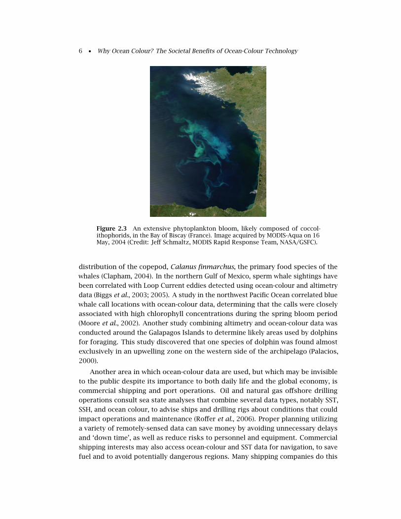
Figure 2.3 An extensive phytoplankton bloom, likely composed of coccol-ithophorids, in the Bay of Biscay (France). Image acquired by MODIS-Aqua on 16May, 2004 (Credit: Jeff Schmaltz, MODIS Rapid Response Team, NASA/GSFC).
distribution of the copepod, Calanus finmarchus, the primary food species of the
whales (Clapham, 2004). In the northern Gulf of Mexico, sperm whale sightings have
been correlated with Loop Current eddies detected using ocean-colour and altimetry
data (Biggs et al., 2003; 2005). A study in the northwest Pacific Ocean correlated blue
whale call locations with ocean-colour data, determining that the calls were closely
associated with high chlorophyll concentrations during the spring bloom period
(Moore et al., 2002). Another study combining altimetry and ocean-colour data was
conducted around the Galapagos Islands to determine likely areas used by dolphins
for foraging. This study discovered that one species of dolphin was found almost
exclusively in an upwelling zone on the western side of the archipelago (Palacios,
2000).
Another area in which ocean-colour data are used, but which may be invisible
to the public despite its importance to both daily life and the global economy, is
commercial shipping and port operations. Oil and natural gas offshore drilling
operations consult sea state analyses that combine several data types, notably SST,
SSH, and ocean colour, to advise ships and drilling rigs about conditions that could
impact operations and maintenance (Roffer et al., 2006). Proper planning utilizing
a variety of remotely-sensed data can save money by avoiding unnecessary delays
and ‘down time’, as well as reduce risks to personnel and equipment. Commercial
shipping interests may also access ocean-colour and SST data for navigation, to save
fuel and to avoid potentially dangerous regions. Many shipping companies do this

Ocean-Colour Radiometry and the Public • 7
routinely, but one of the most visible applications of this technology was during the
Volvo Ocean Race in 2001-2002, when round-the-world yacht racing crews referred
to ocean-colour and SST data to plot their fastest course (IOCCG, 2001). Since each
yacht in the race required a substantial investment from several corporate sponsors,
gaining even a small speed advantage from an accurate analysis of ocean currents
was a requirement to attract news coverage and the prestige of leading a leg of the
race, or eventually winning the globe-girdling challenge.
One of the advanced applications of ocean-colour data is for the detection and
quantification of marine suspended sediments (Fig. 2.4, see also Section 7.4), and
for the observation of changes in bottom topography caused by sediment transport.
Sediments can either alter the course of, or reduce the depth of, shipping channels,
and so the impact of sediment movement in the vicinity of shipping channels
and ports is a significant concern. Data from SeaWiFS, MODIS and MERIS have
been used to monitor the movement of sediments in several port areas and river
estuaries (Hesselmans et al., 2000; Ruddick et al., 2003). Sediments mobilized either
Figure 2.4 A satellite view of the Bangladesh coastline showing the dischargeof sediments from the mouths of the Ganges River. Image acquired by ESA’sMERIS sensor on 8 November 2003. (Credit: European Space Agency).
by dredging or by natural processes such as winds and bottom currents can be
deposited on vital benthic habitats such as seagrass beds, reducing or destroying the
viability of the habitat. This impact can detrimentally affect marine life, as seagrass
and similar aquatic vegetation habitats are frequently inhabited by larval fish and
crustacean species that are commercially and recreationally desirable. In one study,
8 • Why Ocean Colour? The Societal Benefits of Ocean-Colour Technology
remote sensing data from several different sensors (Landsat, ASTER, MODIS) are
being used to analyze the distribution of seagrasses in Florida Bay and the impact of
harmful blooms of blue-green algae. This study is part of the United States Geological
Survey’s Priority Ecosystems Science program, focused on South Florida ecosystem
restoration.
The capability of accurately observing the topography of the sea floor in shallow
waters is also an important area of research for military applications. Water clarity
is a significant concern for the detection of mines, for operations by divers intended
to detect and neutralize mines, and to determine where such operations would
be likely to succeed. Weidemann et al. (2004) describe the use of satellite ocean-
colour data to deliver water clarity information in support of diving and de-mining
operations during hostilities in the Middle East (see also Section 7.2). Advanced
optical analysis of the water column and bottom characteristics is useful for port
protection, detection of objects and/or changes in objects on the sea floor, and
assessment of organic and inorganic particulate matter in the water column for
water clarity prediction (Hou et al., 2002; Carder et al., 2003).
Predictive and forecast uses of ocean-colour data continue to be developed. The
NOAA Red Tide Forecast System for the Gulf of Mexico mentioned above is an
early example of this type of application. Many other uses have been envisioned
for ocean-colour data in forecast and prediction modes. Because ocean-colour
data is well-suited for detection of convergence zones and oceanic fronts, the data
could be utilized for the prediction of the movement and potential coastal impact
of stinging jellyfish and siphonophores, such as the Portuguese man-of-war and
Australia’s lethal box jellyfish. NOAA has implemented a sea nettle prediction system
for the Chesapeake Bay based on the relationship between sea nettle distribution,
salinity, and SST (Decker et al., 2007). Similar systems could utilize ocean-colour
data provided significant relationships between ocean-colour features and areas of
potential occurrence of stinging and/or poisonous species can be reliably determined.
Beach and coastal areas are increasingly susceptible to hazardous conditions
due to high bacterial levels in the water. Such conditions can be caused by excessive
storm-water and sewage release, and can cause associated phytoplankton blooms
(Fig. 2.5). High bacterial levels can cause various intestinal and diarrhoeal diseases.
Ocean-colour data can be utilized in monitoring mode to observe water quality
and water clarity conditions (see Chapter 7), and could also be used for short-term
prediction of conditions requiring beach closure for public safety.
The association of cholera outbreaks with phytoplankton blooms is well-known
(Colwell, 1996). Due to this association, ocean-colour data have been used in studies
of the linkages between the terrestrial and aquatic ecosystems in areas where cholera
outbreaks occur regularly (Lobitz et al., 2000). This type of study seeks to determine
the relationship between climate and infectious diseases such as cholera, and to
predict the influence of climate change on disease progression and transmission in
coming decades.

Ocean-Colour Radiometry and the Public • 9
The uses described above for ocean-colour data mainly address the many ways in
which the public utilizes ocean resources, both directly and indirectly. Another aspect
of ocean-colour data that will become increasingly important is in oceanographic
and geoscience education. Tools such as the SeaWiFS Data Analysis System (SeaDAS)
Figure 2.5 MODIS-Aqua image acquired on 12 August, 2003 showing a brightfeature emanating from the city of Algiers on the Mediterranean coast of Africaa few days after torrential thunderstorms. This feature likely consists ofphytoplankton utilizing nutrients in the runoff plume, as well as components ofsewage and suspended sediments. (Credit: Jacques Descloitres, MODIS RapidResponse Team, NASA/GSFC).
(Fu et al., 1998) and the Goddard Earth Sciences Data and Information Services
Center (GES DISC) Interactive Online Visualization and ANalysis Infrastructure
("Giovanni") (Berrick et al., 2004; Acker et al., 2005; Acker and Leptoukh, 2007)
provide pathways for students to understand the oceanic environment - and perform
research on it - using actual data. These tools, along with simpler methods to access
and acquire data for specific topical research, allow a wider cross-section of the
educational community to utilize the data for classroom instruction and ‘hands-on’
research project investigations. These tools open a previously-closed window on
understanding basic oceanic processes, and also serve to instruct students on how
scientists employ the data to gain insight on oceanic processes and physical-biological
interrelationships. In addition to the tools, the creation of uniform, single format,
multi-mission data sets covering several decades will allow even greater access to
the data, and the discovery of relationships and trends that cannot be discerned in
shorter-term data sets. Because undergraduate and high-school students will find
and use the data in their classrooms, the general public (i.e., parents) will also be
exposed to, and develop increased awareness of, the usefulness and ubiquity of
ocean-colour data in science and in the world community.

10 • Why Ocean Colour? The Societal Benefits of Ocean-Colour Technology
The world population is presently concerned with the issue of climate change,
and the contribution of mankind’s activities to the state of the current climate and
future climate trends. Ocean-colour data is an important element in understanding
how the oceans’ biological systems respond to climate forcing and climate variability,
and how they may change in the future in response to alteration of the global climate
(see Chapter 10).
Although ocean-colour sensors usually acquire data at moderate spatial reso-
lution, in general ranging between 1- and 10-km pixel size, the imagery provides
excellent large-scale views of weather systems and the response of the ocean to
significant weather events (see Chapter 9). Hurricanes and typhoons, in particular,
are unmistakable features in ocean-colour imagery. Observations of hurricanes have
revealed several different aspects of their interaction with the oceanic environment.
The high surface winds of a hurricane stir the water column, bringing dissolved
coloured organic matter and nutrients to the surface and creating detectable ocean-
colour features (Hoge and Lyon, 2002; Shi and Wang, 2007). When hurricanes
encounter the coast, the winds cause re-suspension of coastal sediments, which can
be carried offshore (Acker et al., 2002). Inland flooding caused by the heavy rains of
a hurricane can lead to significant transport of terrigenous sediments offshore in
days subsequent to the passage of the storm. These effects are not caused solely by
hurricanes; elevated winds and rain from more conventional storms and "nor’easters"
can also re-suspend sediments, and cause flooding and increased offshore sediment
transport (Mertes and Warrick, 2001).
Other effects of weather are more subtle, and more seasonal. When the oceans
warm up and sunlight increases in the spring, many oceanic regions witness the
occurrence of the annual ‘spring bloom’, a marked increase in phytoplankton
populations caused primarily by the increased availability of nutrients and increased
sunlight. The timing and magnitude of this event is critical to many important
species of fish, including commercial species (Platt et al., 2003) (see Chapter 8).
Other areas where the influence of seasonal weather patterns is clearly observable
in ocean-colour imagery are the Arabian Sea, where the monsoon causes a dramatic
increase in phytoplankton activity, and the Pacific Ocean coast of Central America,
where powerful winds jetting through mountain passes, caused by winter weather
systems in the Caribbean Sea, mix nutrients to the surface and foster the productivity
necessary for commercial and sport fishing in that region.
Although the effects of weather on the ocean generally occur over short time
periods ranging from days to weeks, the effects of climate variability and climate
change on the oceans can be observed only over periods of months to years. One of
the first observations of the interaction of climate processes and the oceans occurred
when the Coastal Zone Colour Scanner (CZCS) documented the biological effects of
the large El Niño event occurring in 1982-1983 (Feldman et al., 1984). CZCS data
indicated that phytoplankton pigment concentrations in the Equatorial Upwelling
Zone, particularly near the Galapagos Islands, were markedly diminished during this

Ocean-Colour Radiometry and the Public • 11
El Niño event. The observations confirmed that El Niño caused widespread changes
in the biological dynamics of the Pacific Ocean. Under serendipitous circumstances,
the launch of SeaWiFS in September 1997 coincided with the onset of another major
El Niño event, which peaked in strength from November 1997 through May 1998.
The nearly-continuous coverage of SeaWiFS allowed the observation of the strong
cessation of biological activity in the Equatorial Upwelling Zone, and the remarkably
rapid restoration of the upwelling and increased chlorophyll concentrations in June
and July 1998 (Chavez et al., 1998) (Fig. 2.6). The shift from El Niño to subsequent La
Niña conditions caused a major shift in the uptake of carbon by the oceanic system
(Behrenfeld et al., 2001). El Niño and La Niña, also known as the El Niño Southern
Figure 2.6 SeaWiFS images of the Pacific Ocean during the peak of the 1997-1998 El Niño (top), during which phytoplankton activity in the EquatorialUpwelling Zone was significantly reduced, and (bottom) during the subsequent LaNiña when phytoplankton activity in the Equatorial Upwelling Zone was elevated(Credit: SeaWiFS Project, NASA/Goddard Space Flight Center and GeoEye).
Oscillation (ENSO) events, are probably the best-known recurring cyclic phenomena
in the ocean, due to their widespread impact on Pacific Ocean regions, including
the coasts of Central and South America, Indonesia, Polynesia, and Australia. Other
cyclic phenomena that produce recurring patterns of interannual variability are the
Pacific Decadal Oscillation (PDO), the North Atlantic Oscillation (NAO), and the Arctic
Oscillation (AO). Sea surface height data, SST data, ocean surface wind data, and
ocean-colour data are all remotely-sensed data products that provide diagnostic

12 • Why Ocean Colour? The Societal Benefits of Ocean-Colour Technology
criteria allowing scientists to evaluate the dominant modes of these phenomena.
As the data records become longer, it becomes possible to examine the recurrence
frequency of these events and relate their frequency to the affects of climate change.
The accuracy of remotely-sensed data is, however, one of the primary concerns
in the compilation of multi-decade climate data records (CDRs). Each satellite Earth-
observing sensor is unique, even despite the best technological efforts to produce
duplicate instruments, such as the Advanced Very High Resolution Radiometer
(AVHRR). For ocean-colour data, the problem is more acute, as to date there has
not been a ‘series’ of similar instruments primarily dedicated to ocean-colour
observations. Merging the data from different sensors therefore presents a data
processing and data analysis challenge. Initial efforts in this regard have indicated
distinct trends in the chlorophyll concentration of the world’s oceanic basins from
the CZCS observational period in 1978-1986 to the present (Dutkiewicz et al., 2001;
Gregg and Conkright, 2002; Gregg et al., 2003; 2005). NASA funded the Ocean Colour
Time-Series Project to determine if CZCS and OCTS data could be reprocessed in a
manner emulating, as closely as possible, the data processing methodology applied
to SeaWiFS and MODIS-Aqua data by the Ocean Biology Processing Group (OBPG) at
NASA GSFC. This effort indicates the difficulty of connecting disparate data sets into
CDRs due to differences in sensor performance and operating conditions. Another
merged data set is the ESA DUE GlobColour multi-parameter data set based on
SeaWiFS, MERIS and MODIS data (see http://www.globcolour.info). The merging of
data from individual sensors not only provides a long time-series, but also increases
the temporal coverage and error characterisation of the final data set (see Section
10.3). The combination of the three sensors allows about 30% of the ocean to be
covered on a daily basis (IOCCG, 1999).
In the 1960s, consultation of images from the first generation of weather satellites
to improve forecasting was a pioneering endeavour, though we now consider such a
practice commonplace and necessary. At the end of the first decade of routine ocean-
colour observations, the increased use of ocean-colour data in applications that are
directly related to the public interest is becoming more evident. It is certain that
future ocean-colour radiometry missions will provide data addressing an increasing
variety of topics where the interests of the scientific research community and the
public would derive mutual benefit - a significant reason to invest in the continuation
of accurate ocean-colour remote sensing from space.
Chapter 3
Ocean-Colour Data - An Aid to Modelling
Ian Robinson
In many branches of oceanography numerical simulation is an important tool for
research and operations. For example, research on climate change is strongly
dependant on models, including models of the ocean carbon cycle. Simulating the
role of the ocean on the Earth’s carbon cycle needs an ecosystem model embedded in
a general circulation model. For any model that purports to represent the large-scale
features of the ocean, we require data from Earth observation to accomplish at least
two information tasks: the provision of data fields for model initialization and for
model validation. In this section the important role of ocean-colour data as an aid
to modelling is discussed.
The use of satellite ocean-colour data in the context of numerical ocean models is
a steadily developing field of study which is leading towards a variety of research and
operational applications. It is not really a separate category of use, but rather should
be viewed as the means by which a number of the applications of ocean-colour data
discussed elsewhere in this document can be enhanced, or extended into operational
situations. This section will first review the circumstances where ocean models can
benefit from ocean-colour data and vice versa. It will then outline the different ways
in which colour-derived ocean properties, normally the near surface concentration
of chlorophyll-a, are assimilated or otherwise used to improve the predictions of
ocean models. Finally, it will consider the implications for the co-ordinated planning
of ocean-colour monitoring systems by different space agencies, if their data are
required for operational models.
3.1 When Are Ocean-Colour Observations Used in Models?
In most applications of ocean colour, the satellite data provide the primary
information about a particular ocean phenomenon or process. Ocean-colour data by
itself, or in combination with observations of other ocean properties, is sufficient
to present a clear story. But this is not always the case. What are the situations
where the colour data need to be linked to the use of a numerical model? We can
identify two types of use: the first is where a model is required to improve scientific
13
14 • Why Ocean Colour? The Societal Benefits of Ocean-Colour Technology
understanding, the second is where the model is needed in support of operational
monitoring.
3.1.1 Model to Represent Scientific Complexity
In the first case, the subject typically requires the complex interactions between
many parameters, including ocean colour, to be defined and a numerical model
is used to do this. The parameters in the model need to be tuned to make it as
realistic as possible in order to increase the confidence that can be placed on the
results gained from running the model. An obvious example is that of ecosystem
models capable of representing the growth and decay of a phytoplankton bloom
in the ocean. Although the chlorophyll measurements obtained from ocean-colour
data are able to show when and where blooms occur, this by itself is not sufficient
to understand the processes. It needs a biochemical model of the balance between
primary production, nutrient supply and grazing by zooplankton to be embedded in
a physical/dynamical model describing circulation, mixing and upwelling, before we
can begin to represent the complex interactions that constrain this most important
of all oceanographic processes.
Ecosystem models of the open ocean that truly represent the distribution of
primary producers in three spatial dimensions and time are needed to be able to
answer a number of important scientific questions about, for example: the ratio of
new to regenerated production; the proportion of carbon fixed by primary production
that is exported from the surface layer; the impact of a phytoplankton bloom on
the pCO2 at the ocean surface and hence on the exchange of CO2 between the
ocean and atmosphere. These and similar questions need a reliable biogeochemical
model embedded in a physical model to enable us to reach answers that account
for the space-time variation of the real ocean. Satellite-derived observations of
chlorophyll by themselves cannot answer these questions. Neither can a model
do so by itself because without comparison against actual observations the model
parameters cannot be tuned. Independent observations are also needed to evaluate
the tuned or calibrated model with regard to its generality and reliability. Although
in situ measurements are of some value, only satellite colour data can provide the
high-resolution view of spatial structures, the wide area coverage and the repeated
sampling over time to capture the detailed evolution of a phytoplankton population
that is required to constrain the model parameters. Thus only a combination of
satellite data and numerical models can answer some of today’s key oceanographic
questions.
In coastal seas the situation is even more complex than in the open ocean,
and the use of models is even more essential. Here the additional factors of land-
derived dissolved organic material, re-suspended bottom sediments or river borne
particulates not only create the Case 2 optical conditions (IOCCG, 2000), but also
add complexity to the biogeochemical processes. The potential of satellite ocean-

Ocean-Colour Data - An Aid to Modelling • 15
colour data to yield information about suspended sediments and CDOM as well
as chlorophyll is very attractive, but can only be realised when the challenge of
interpreting Case 2 data has been solved.
3.1.2 Model to Meet Operational Needs
In the second type of use, models are needed in conjunction with satellite ocean-
colour data primarily because information about the ocean needs to be supplied for
operational purposes. Take, for example, the operational responsibility of warning
coastal holiday resorts about the occurrence of algal blooms which interfere with
maritime leisure activities. Satellite data alone can be adequate for this task, but
only if daily cloud-free cover is available. Since this can rarely be guaranteed, the
authorities with operational responsibility are unable to rely exclusively on the
satellite data. In these circumstances the use of a model capable of predicting the
evolution and movement of algal blooms, regularly updated by satellite observations
when skies are clear, offers an effective solution. Of course the model that is used
might be very similar to one of the models discussed in the previous paragraph,
but here it serves a different purpose. The combination of satellite data, in situ
measurements and numerical model is conceived as an operational ocean or coastal
‘observing system’, in which the output of the model provides the best available
estimate of the state of the ocean at a given time. The model effectively fills in the
gaps, in space and time, between all the available observations. Typically it provides
a ‘nowcast’, and if the system offers a modest capacity for forecasting, then that is a
bonus.
It is not only tourism that needs such integrated observing systems but also
the marine aquaculture industry and those with a statutory responsibility for water
quality monitoring. As international legislation imposes greater demands on nations
to monitor the quality of the water in their own exclusive economic zones (EEZ),
ocean observing systems are increasingly seen as an essential tool. Although in most
cases ocean colour is used to provide information about biogeochemical aspects of
the sea, the use of ocean colour radiometry data as a tracer of water movement and
water masses should not be overlooked. There are circumstances where knowledge
of ocean surface currents is needed at fine spatial resolution, for example in order to
supply information crucial for the planning of difficult offshore drilling operations.
In these circumstances both ocean colour and temperature images can provide
evidence of the smallest mesoscale features, but their assimilation in a dynamical
model is essential to provide operational reliability in all weathers.
It is important to distinguish between what we may call the scientific and
the operational model cases because they impose different requirements on the
timeliness with which processed satellite data are provided to users, and on the
continuity and sustainability of ocean-colour missions. These will be discussed in
the final part of this section.

16 • Why Ocean Colour? The Societal Benefits of Ocean-Colour Technology
3.2 Confronting Models with Ocean-Colour Radiometry Data
3.2.1 The Basic Modelling Principles
The numerical models that have so far been adapted to assimilate satellite ocean-
colour data are ecosystem models of varying complexity. For application in the
open ocean, relatively simple pelagic ecosystem models are used, based largely on
the approach pioneered by Fasham et al. (1990) and Fasham (1993). In Fasham et
al. (1990) the ecosystem is separated into seven separate compartments. Using
nitrogen as the basic currency of the model, each compartment is defined in terms
of the amount of nitrogen per unit volume (mmol N m−3). The seven compartments
are; phytoplankton (P), zooplankton (Z), bacteria (B), nitrate, ammonium, dissolved
organic nitrogen (DON), and detritus as non-living particulate organic nitrogen (PON).
The model equations represent the applicable biological processes within a single
model element for P, Z and B, such as primary production, respiration, grazing,
excretion and mortality. There are many variants involving more or less than seven
nitrogen pools. In some cases additional variables are introduced to represent the
carbon partitioning and the alkalinity (Drange, 1996).
When the ecosystem model is embedded within a three-dimensional ocean
circulation model, additional equations represent the transport of the different
ecosystem components between the model grid cells by advection, diffusion, or
sinking under gravity. A variety of different basin-scale models have been developed,
using slightly different ecosystem and chemical models attached to different types
of ocean circulation models, some with fine enough spatial resolution to resolve
mesoscale eddies. They have been created for the North Atlantic (Drange, 1996;
Gunson et al., 1999; Oschlies and Garçon, 1998; 1999; Oschlies et al., 2000), the
tropical Pacific (Christian et al., 2002) and the global ocean (Gregg, 2001; Palmer and
Totterdell, 2001).
A critical challenge is to determine appropriate values for the parameters used
in each model expression to represent a biological or chemical process. This
requires a calibration procedure which optimises the model parameters to match an
independent set of observations. Although local ecosystem models can be tuned
for a particular place and season using a suite of in situ measurements of the
main ecosystem components, parameter sets determined in this way can not be
applied with confidence to a basin-scale model running throughout the year. In that
case, chlorophyll data obtained from satellite ocean colour can provide the global
geographical coverage, the spatial detail and most importantly the multiple annual
cycles needed to represent the variety of conditions which such a model must be
capable of simulating. Parameter estimation is the motivation behind most of the
assimilation work reported so far.
In shelf seas where there is greater heterogeneity of the pelagic ecosystem
over shorter length scales, and where benthic processes must also be taken into

Ocean-Colour Data - An Aid to Modelling • 17
account, modellers have used more complex designs, such as the European Regional
Seas Ecosystem Model (ERSEM), which has been applied to the North Sea, the
Mediterranean Sea, the Adriatic Sea and the Arabian Sea (Allen et al., 2001). The
marine ecosystem is represented by a network of physical, chemical and biological
processes organised within pelagic and benthic components. In these more complex
models the biota are necessarily segregated into functional groups that are intended
to represent particular types of behaviour rather than species lists. Each functional
group is defined by a number of explicitly-modelled components: carbon, nitrogen,
and phosphorous and, in the case of diatoms, silicon. In ERSEM phytoplankton
are represented by four functional types: picophytoplankton (0.2-2 µm), small
autotrophic flagellates (2-20 µm), large autotrophic flagellates (20-200 µm) and
diatoms (20-200 µm). When embedded into a three-dimensional physical model
of a shelf sea, there are 36 pelagic state variables to be advected and diffused by
the hydrodynamics. It is essential to establish valid parameterizations for each of
the many processes if the model is to have a predictive capability. This is where
modellers look to satellite ocean-colour data to provide time-evolving distributions of
chlorophyll, and possibly also dissolved organic material and suspended particulate
matter, against which to test and calibrate their parameterizations, and ultimately
validate the model.
3.2.2 Experience with Assimilating Chlorophyll in Ecosystem Models
When using satellite-derived chlorophyll data for calibrating and validating models,
there are three important factors to be noted because they are potentially limiting.
v Some ecosystem models do not use the concentration of chlorophyll-a (Chl-a)
as an explicit model variable. In such cases the dependence of Chl-a (mg m−3)
on the magnitude P (mmol N m−3) of the phytoplankton compartment of the
model must be established, for example as characterised by the Michaelis-
Menten relationships (Michaelis and Menten, 1913). The form proposed by
Semovski and Wozniak (1995) is:
P = ρmaxChla2
(Chla +K1/2)R, (3.1)
where ρmax is 90 mol C per g Chl and the half saturation constant, K1/2, is
0.477 mg m−3. R is the Redfield ratio to convert the expression from carbon
to nitrogen units (taken to be 6.625 for the deep ocean). Before assimilation an
expression such as this must be used to convert satellite-derived chlorophyll
data into the model representation of phytoplankton, or vice versa.
v Satellite data provide observations of only one of the seven biogeochemical
compartments used by the Fasham-type models.
v The typical accuracy of Chl-a retrieved from ocean colour is 35% in open
seas and even poorer in Case 2 conditions. This compares unfavourably

18 • Why Ocean Colour? The Societal Benefits of Ocean-Colour Technology
with the accuracies of sea surface height anomaly and temperature, which
are the satellite measurements used for assimilation into numerical models
representing ocean physics and flow dynamics
However, when Natvik and Evensen (2003 a; b) developed techniques to assimilate
SeaWiFS data into a full three dimensional ecosystem model embedded in a North
Atlantic hydrodynamic model, they were able to demonstrate that the satellite data
measurably improved the model response. This model uses an ensemble Kalman
filter (EnKF) approach to assimilation. Using the satellite data reduced the variance
fields for all the variables, including those partitions of the ecosystem that were not
directly observed. They concluded that the use of a multivariate analysis scheme
enabled the phytoplankton information supplied by the satellite data to improve the
analyses for the other ecosystem partitions. This result confirms the relevance of
satellite ocean-colour data for future biochemical ocean model developments.
Hemmings et al. (2003; 2004) used SeaWiFS-derived chlorophyll data from
locations across the North Atlantic to calibrate a zero-dimensional plankton
ecosystem model (that is, one that is not embedded within a circulation model
but which attempts to describe the seasonal cycle separately at a number of different
locations). The aim was to achieve this using a single set of parameters. They
concluded that the derived parameter sets are improved by using the satellite data
because the high volume of observed data can supply examples of a wide range of
possible biogeochemical responses to different physical conditions. For the same
reason they demonstrated that the model performance is improved if the north
Atlantic is divided into two provinces for which the parameters are independently
calibrated. However, they introduce a note of caution, observing that despite the
advantage of using satellite chlorophyll for calibrating the model, the parameters
remain poorly constrained without observations of the other ecosystem elements.
3.3 Operational Models Using Inputs of Satellite Ocean-ColourData
The ecosystem models mentioned above are concerned with improving the scientific
understanding of ecosystem processes. However, increasing operational use is being
made of ecosystem modules embedded in physical circulation models to provide
forecasts of the development of plankton blooms, in order to issue warnings of
harmful algal blooms (HAB) or the risk of eutrophication in vulnerable sea areas. One
example of how such a model makes use of satellite ocean-colour data is provided
by Svendsen et al. (2004), in a case study describing the operational monitoring for
a HAB of Chattonella spp. This species started to bloom in Scandinavian waters in
1998, returning in 2000 and 2001, killing thousands of tons of farmed salmon along
the southern Norwegian coast. The study describes the real-time monitoring of the
bloom in 2001, using SeaWiFS data.

Ocean-Colour Data - An Aid to Modelling • 19
At the heart of the monitoring process is an ecosystem model embedded in a
hydrodynamic model of the Norwegian coastal seas, relying on observational data
inputs to achieve a good representation of the real ocean, but still able to provide
estimates of the ocean state at times and locations when no observations are available.
Every cloud-free chlorophyll image is compared with the model phytoplankton
prediction. When a bloom event is detected by the satellite but is not predicted by
the model, the model phytoplankton field is manually re-initialised to the observed
concentrations following the spatial distribution from the satellite image. The model
then continues to predict the further development, advection and final decay of
the bloom and warnings are issued if the bloom approaches the coast. Subsequent
satellite observations are used just for validation, and further re-initialisation is
performed only if the model output deviates badly from the satellite estimates.
The model includes as state variables the abundance of two functional groups,
diatoms and flagellates, but does not specifically represent a particular harmful algae
species. Therefore when a bloom is detected from space, in situ samples are urgently
needed to determine whether it is a harmful species or not. Despite the obvious
shortcomings that the HAB species are neither represented explicitly in the model
nor directly distinguishable from non-harmful species in satellite ocean-colour data,
this case study demonstrates how effective can be the combination of model, satellite
data and in situ sampling for critical operational tasks. Although the assimilation
technique is fairly crude, it is effective and adequate for the operational task.
3.4 Alternative Approaches
The assimilation of satellite data into ecosystem models is still at an early stage of
development but shows promise, especially in the open ocean where the measurement
of Chl-a from space is generally reliable. However, in coastal waters, where the
requirement for observations is amplified by the complexity of the ecosystem model,
the methodology of parameter retrieval from ocean colour is compromised by the
ambiguity of Case 2 conditions. One of the difficulties with the interpretation of
Case 2 ocean-colour images is not knowing the relative contribution of chlorophyll,
CDOM and SPM which can, independently, affect the colour. However, when satellite
data are being used for assimilation in support of a model, then the model may have
some skill in predicting in advance what the balance is likely to be between the three
possible colour-controlling constituents. This points towards the possibility of an
interactive approach to Case 2 algorithms using the ecosystem model forecasts.
Taking this line of thinking further, a more radical approach would be to use
the model to predict the colour of the sea (i.e. the reflectance in each spectral
band) and to compare this directly with what the satellite observes, as discussed
by Robinson and Sanjuan-Calzado (2006). This would eliminate the need for the
relatively uncertain inversion of the colour data to retrieve chlorophyll or SPM or

20 • Why Ocean Colour? The Societal Benefits of Ocean-Colour Technology
CDOM. Although some progress has been made in this direction (Fujii et al., 2007),
it remains to be determined whether an assimilation technique can be developed
which is able to adjust the model ecosystem state variables in order to shift the
model’s colour predictions closer to the satellite observations.
3.5 The Implications of Using Ocean-Colour Operationally
The emerging use of ocean-colour data for assimilation in ecosystem and/or ocean
dynamical models, and the potential for supporting operational ocean monitoring
systems by this means, implies a growing dependence of users on the agencies who
provide ocean-colour sensors in space. As more routine use is made of satellite-
derived chlorophyll data, users will look to the agencies to provide continuity of
ocean-colour missions, with new sensors ready to replace old ones into the indefinite
future. Operational users will also look for increased speed of processing and a
reduction in the delivery time between data acquisition and the supply of a processed
product. Despite the promise of benefits from using ocean-colour data in support
of ecosystem models, many operational ocean forecasting agencies may hesitate to
set up operational systems until they can be reasonably sure of the continuity of
data provision and the timeliness of delivery.
Moreover, in the same way that data from different satellite altimeters are being
supplied in a co-ordinated way (through the DUACS1 programme) and standards for
harmonising SST data from diverse satellite sensors have been set (by the GHRSST2
project), so there is a growing demand from users for a harmonised set of ocean-
colour products. Modellers and operational users simply want to obtain the most
recently acquired observations of chlorophyll or other colour-related products from
space. It is seen as an unnecessary complication if they have to interpret products
from different agencies in different ways. For serious assimilation, an error estimate
needs to be supplied with each measurement. Ideally all data should be supplied
in a common and readily accessible format. Finally some users may prefer a single
merged, averaged or blended global daily chlorophyll observation derived from all
available ocean-colour sensors. This issue was the topic of a recent IOCCG report
(IOCCG 2007) and is currently being addressed by the ESA GlobColour Project 3.
1DUACS - Developing Use of Altimetry for Climate Studies system based at CLS which merges datafrom T/P and Jason-1, Envisat/ERS-2 and GFO altimeters to produce along-track data and Maps ofSea Level Anomalies (MSLA) on a near-real time basis. (See http://www.jason.oceanobs.com/html/donnees/duacs/welcome_uk.html
2GHOSTS - Global ocean data assimilation experiment High-Resolution Sea Surface Temperaturepilot project. (See http://www.GHRSST-PP.org)
3For more information on GlobColour see: http://www.globcolour.info/index.html

Chapter 4
Ocean-Colour Radiometry and Ocean Physics
Stephanie Dutkiewicz, Robert Frouin, Shubha Sathyendranath andB. Mete Uz
4.1 Introduction
Physical processes in the ocean dictate largely the chemical and light environment in
which the phytoplankton find themselves. Growth of phytoplankton at sea requires
light and nutrients. The average light experienced by the phytoplankton in the
mixed layer of the ocean depends on the light reaching the sea surface, the rate
of light attenuation with depth in the water column, and the depth of the mixed
layer itself. In most areas of the world ocean, the supply of nutrients into the mixed
layer depends on various physical processes: advection, diffusion and mixing. Thus,
the distribution of phytoplankton in the surface mixed layer is intimately linked to
the physical processes. Many of these processes are transient, and remote sensing
has played a very useful role in providing evidence for the importance of transient
processes in sustaining ocean productivity, which in turn has stimulated modelling
studies designed to pinpoint the underlying physical mechanisms responsible for
the observed biological features.
On the other hand, the growth of phytoplankton at sea modifies the light field
underwater. In fact, in open-ocean waters, phytoplankton and associated material are
recognised to be the most important factor responsible for modifying the underwater
light field. The changes in the properties of light penetration in turn modifies the
rate of solar heating at various depths in the ocean (Fig. 4.1), altering water-column
stability and hence mixed-layer dynamics. Studies of such feedback mechanisms by
which biological properties modulate the physical processes have also been given an
impetus by the availability of ocean-colour data appropriate for such studies.
In this chapter, we summarise ocean-colour applications in studies of physical
processes that influence phytoplankton dynamics at sea, and biological feedback
mechanisms.
21

22 • Why Ocean Colour? The Societal Benefits of Ocean-Colour Technology
Figure 4.1 Schematic diagram showing links between diffuse attenuationcoefficient K and mixed-layer depth. Small values of K would be associated witha weak vertical gradient in solar heating. Therefore, other things being equal,low values of K would favour deeper mixing, compared with waters where K ishigh.
4.2 Effect of Physical Processes on Fields of Phytoplanktonand Primary Production
Ocean spectral reflectance in the visible domain is the only optical signal open
to biological interpretation that is measured over the global ocean at resolutions
comparable with the suite of physical properties observed by remote sensing, such
as SST, SSH, wind vectors and precipitation. Consequently, it is often co-analyzed
with one or more of these variables to elucidate mechanisms of physical-biological
coupling in the ocean.
In the well-lit upper ocean, phytoplankton rapidly assimilate available nutrients
into biomass. When particulate organic material falls out to deeper layers, nutrients
incorporated into the material are also lost with it. For continued productivity in
the upper ocean, this loss must be compensated by either atmospheric sources, or
by the injection of nutrient-rich waters from below. Except for micronutrients such
as iron, atmospheric deposition is generally not very important. And, as the water
column is stably stratified over much of the ocean, the background level of nutrient
supply through vertical mixing of denser nutrient-rich waters is very limited.
Much of the observed variability in phytoplankton biomass and productivity
occurs as a result of processes such as winter mixing and coastal or equatorial
upwelling which bring nutrients from deeper layers to the surface. However, at places
such as the interior of subtropical gyres, as characterized by the Bermuda Atlantic
Time Series site, primary productivity has been observed to be higher than can be
accounted for by upwelling and vertical mixing, implying additional mechanisms

Ocean-Colour Radiometry and Ocean Physics • 23
of nutrient replenishment. Numerical modelling and, most recently, shipboard
observations have shown that processes associated with baroclinic disturbances
can be a significant source of additional nutrients and thus support a significant
increase in productivity.
4.2.1 Spring Bloom Dynamics
Phytoplankton blooms in the North Atlantic are some of the most pronounced of
any open ocean region. Although this region and its immense seasonal blooms have
been the subject of many investigations over the years, it was only with the advent
of satellite ocean-colour data that we have been able to investigate the temporal and
spatial variability of these blooms. One of the strongest controls on interannual
variability in the blooms appears to be from meteorological modulation (Townsend
et al., 1992; Follows and Dutkiewicz, 2002; Lévy et al., 2005; Ueyama and Monger,
2005).
Bloom dynamics involve a delicate balance between nutrient supply and light
limitation. The latter is regulated by seasonal progression of the sun, but also
significantly by the depth of the mixed layer (Sverdrup, 1953). If the mixed layer
is too deep, phytoplankton will on average have too little light and growth will be
impeded. Yet, a deeper mixed layer (stronger convective events) leads to entrainment
of higher concentrations of nutrients from below. In fact, Dutkiewicz et al. (2001)
showed, using model simulations, that vertical mixing can enhance productivity
by supplying nutrients from below, but can also decrease productivity by mixing
phytoplankton below the critical depth (here defined as the depth above which, in
the absence of nutrient limitation, there is a net growth in phytoplankton).
It is only with detailed satellite ocean-colour studies that these patterns become
more clearly and broadly visible. There is a difference in behaviour in bloom
variability and indicators of mixing in the subtropical and subpolar regimes (Follows
and Dutkiewicz, 2002). In the subtropics, enhanced mixing leads to increased
chlorophyll amplitudes, while in the subpolar regions it leads to reduced amplitudes.
Ueyama and Monger (2005) examined the interannual variability exhibited by the
first EOF mode of SeaWiFS ocean-colour data together with SSM/I wind data between
the year 1998 and 2004 in the North Atlantic. These modes exhibited strong spatial
coherency and indicate regions where bloom timings and magnitudes are in phase
and regions where they are out of phase with wind mixing. The southern subtropical
regime showed strong positive correlation between bloom magnitude and wind
mixing. Similarly, there is an out-of-phase relationship in the subpolar regime in
both timing and magnitude of the bloom, supporting the idea of a negative impact of
mixing in this region (Dutkiewicz et al., 2001). Lévy et al. (2005) also find a striking
pattern of an opposite interannual trend in bloom strength derived from SeaWiFS
data and mixed layer depth (provided by a high resolution numerical model) in the
two regimes in the North Eastern Atlantic.
24 • Why Ocean Colour? The Societal Benefits of Ocean-Colour Technology
Even in the subtropical and subpolar regimes the patterns are not always clear,
and there are large tracts of the North Atlantic that do not fall into either of these
two regimes (e.g., Lévy et al., 2005; Ueyama and Monger, 2005). Apart from other
biogeochemical causes of variability, such as nitrogen fixation (Michaels et al., 1994)
and grazing (Popova et al., 2002), there are also other physically-driven mechanisms
that impact bloom variability. For instance mesoscale activity can significantly impact
local supply of nutrients and enhance productivity (e.g., McGillicuddy and Robinson,
1997; Oschlies and Garçon, 1999), and lateral supply of nutrients is crucial in some
regions of the North Atlantic (Williams and Follows, 1998).
There are, however, striking broad patterns in interannual variability in the North
Atlantic bloom that have emerged from ocean-colour studies, and these appear
strongly linked to modulation in the synoptic atmospheric events between years
(Follows and Dutkiewicz, 2002; Levy et al., 2005; Ueyama and Monger, 2005). These
connections lead to some interesting questions regarding the relation to larger scale
patterns of meteorological variability (e.g. the major mode of wind variability is
associated with the North Atlantic Oscillation, NAO) and to longer time-scale climate
change. A characteristic of low NAO is enhanced mixing in subtropical regions; the
discussion above then suggests that blooms may be enhanced in the subtropical
regimes during this phase of the NAO. Uemaya and Monger (2005) also suggest that
the major mode in the timing of the bloom might be linked to the NAO. Further ocean-
colour studies of these and other phenomena will greatly enhance our understanding
of the mechanism underlying the response of the oceans ecosystems to current and
future variability in the climate.
4.2.2 Physical–Biological Interactions associated with Mesoscale Eddies
Baroclinic disturbances are ubiquitous distortions in the depth and slope of isopycnal
lines, often caused by such processes as instabilities and wind stress variability over
space or time. They generally propagate westward as eddies or planetary waves.
They modulate the depth of isopycnal layers by hundreds of metres and the sea
surface height by tens of centimetres.
Even though sea surface height anomalies are typically a few orders magnitude
smaller than isopycnal displacements, they still form the basis of our observations
of baroclinic features because they are detectable by satellite altimeters. The
advent of altimetry allowed for global characterization of planetary waves and
mid- to large-sized eddies in the ocean. Shortly after the launch of SeaWiFS,
when continuous coverage of ocean spectral reflectance started, colour anomalies
propagating westward at typical planetary-wave speeds were observed and shown to
be phase-locked and coherent with sea surface height anomalies. It is still a matter
of debate and active research whether this manifestation of planetary waves in ocean
spectral reflectance is due to new production in response to nutrient renewal, or
passive transport of existing biomass. With analysis of ocean spectral reflectance
Ocean-Colour Radiometry and Ocean Physics • 25
imagery in comparison with other remotely-sensed properties and model results,
a number of hypotheses have been put forward including horizontal advection
of existing background gradients by the planetary wave, concentration of surface
pigments due to the convergence associated with the waves, and the enhanced
visibility of shoaled subsurface pigment maxima to the satellite sensor over the
wave.
Assessing the mechanism for increased pigment concentrations often observed
within eddies is even more complicated than those observed in association with
planetary waves, because unlike waves, non-linear eddies transport water over
considerable distance and time. It appears that the primary effect of eddies is
to transport existing biomass, however this does not preclude biologically-active
mechanisms, since these would be secondary in nature. To the first order, a
geostrophically balanced eddy would simply move the water around. However,
secondary effects, which are more pronounced under external forcing such as
from wind stress, or when the eddy is actively spinning up or down, would
result in significant vertical velocities, which should affect nutrient and pigment
concentrations.
Present satellite instruments are capable of adequately resolving planetary waves
and mesoscale eddies and significant progress should be expected in the near future
with the available data. If a geostationary sensor were available, its capability to
minimize the effect of cloud cover would be very useful for mesoscale process
studies. The higher spatial and temporal resolution would also allow submesoscales
to be resolved, which are particularly important for biological processes because of
the significant vertical motions associated with these scales.
4.2.3 Effect of Storms
Whereas it is relatively straightforward to use in situ observations to monitor the
supply of nutrients to the surface layer through winter mixing, it is much more
difficult to rely on in situ techniques to monitor physical and biological responses
to transient events such as the passage of storms. Remotely-sensed data provide
unprecedented views into the biological consequences of such transient phenomena.
Several authors (Babin et al., 2004, Davis and Yan 2004; ; Fuentes-Yaco et al. 2005;
Platt et al., 2005, Son et al. 2006) have shown, using sequences of ocean-colour images,
changes in chlorophyll concentrations in the surface layers of the sea following the
passage of storms. Using a 3-D ocean circulation model of the Labrador Sea, Wu et
al. (2007) identified two phases in the responses of the biological field to a steadily-
moving storm. The first and immediate response is associated with deepening of the
mixed-layer and redistribution of the chlorophyll biomass in the new mixed layer.
This is followed by a period of inertial oscillation in the wake of the storm which
may last a few days. An even longer-scale response would be associated with the
new nitrogen that is brought into the well-lit mixed-layer as a result of the enhanced

26 • Why Ocean Colour? The Societal Benefits of Ocean-Colour Technology
storm-induced mixing, which would typically lead to enhanced production over a
longer time scale.
Wu et al. (2008b) also studied a summer bloom in the Labrador Sea in 2006 that
appeared as an anomaly compared with the multi-year climatology of the bloom
dynamics in the area (Fig 4.2). Using models they showed that the bloom could be
explained as the biological response to an intense storm in the area. The physical
processes responsible for the phenomenon were entrainment due to mixing, and
Ekman pumping in zones of divergence of wind stress. Both processes brought new
nitrogen into the layer, which led to enhanced primary production in the layer.
Figure 4.2 Composite MODIS images of the central Labrador Sea for (a) 8-15July, 2006 and (b) 16-23 July 2006 (adapted from Wu et al. 2008b). Modelresults showed that the enrichment of nutrients in the euphotic layer and thesubsequent bloom were related to two wind storms in the period 7-10 July 2006.(MODIS data provided by NASA/GSFC).
4.3 Biological Feedbacks on Physical Processes in the Sea
4.3.1 Attenuation of Solar Radiation and Mixed Layer Dynamics
Some sunlight is reflected at the ocean surface because electromagnetic waves
travel slower in water than in air (due to the higher index of refraction of water).
But most sunlight reaching the surface is transmitted into the ocean, where it is
essentially absorbed. Only a small percentage of the transmitted light, typically 2%,
is backscattered to the atmosphere. Unlike non-solar heat fluxes, which act in the

Ocean-Colour Radiometry and Ocean Physics • 27
immediate vicinity of the surface, solar irradiance may reach, and therefore heat,
waters below the mixed layer. Vertical attenuation of sunlight is due to absorption
and scattering by molecules and particles (phytoplankton, sediments) and absorption
by dissolved organic matter. About 95% of sunlight is absorbed in the upper 100 m
of the clearest waters, but sunlight rarely penetrates deeper than a few metres in
coastal turbid waters. Water composition thus affects the vertical distribution of
solar heating, therefore stratification and mixing, and consequently heat exchange
with the atmosphere and circulation patterns.
The importance of water clarity in determining the thermal structure of the
ocean and mixed-layer dynamics was established by Denman (1973). Later Charlock
(1982), employing a one-dimensional climate model with energy balance, noted
that SST increased by 1-2◦C when water was more turbid. Woods et al. (1984)
emphasized the need for accurate calculation of the vertical profile of solar heating
to meet the requirements of climate prediction. They showed that the rate of solar
heating below the mixed layer depends more on water turbidity than on cloud cover.
Sathyendranath et al. (1991), using the Kraus-Turner mixed-layer model, calculated
a biological heating of up to 4◦C per month in the Arabian Sea.
Figure 4.3 Sea surface temperature response to increasing phytoplanktonpigment concentration, C. The one-dimensional mixed-layer model of Price etal. (1986) was used in the simulations. The atmospheric forcing, specifiedfrom the Comprehensive Ocean-Atmosphere Data Set (COADS), corresponds tothe location, and C was constant during the entire year. Solar absorption byphytoplankton was parameterized according to Morel and Antoine (1994). Theamplitude of the SST annual cycle increases as C increases.
Figure 4.3 illustrates the importance of water turbidity in mixed-layer dynamics.
The one-dimensional model of Price et al. (1986) was used to simulate seasonal
changes in the mixed layer at selected locations. Depending on phytoplankton pig-
ment concentration, SST may change by several degrees C. As pigment concentration
increases, SST becomes warmer in summer and colder in winter, i.e., the seasonal
cycle of SST is amplified. More radiation is absorbed in the mixed layer when pigment

28 • Why Ocean Colour? The Societal Benefits of Ocean-Colour Technology
concentration is higher, and less radiation penetrates below the mixed layer. In
winter, the ocean surface is able to transfer heat to the atmosphere more efficiently.
When the mixed layer deepens in winter, it brings up water from below that is cooler
than the water corresponding to lower pigment concentrations, resulting in a cooler
mixed layer.
Figure 4.4 Top: Surface temperature difference between OGCM runs with andwithout phytoplankton-radiation forcing in the Pacific, between 30◦S and 30◦N.Bottom: Vertical profile of temperature along the equator, between the surfaceand 220 m. Surface temperature is generally increased in the entire horizontaldomain, by 0.1 to 0.5◦C, except in a relatively narrow latitude band along theequator between 180 and 100◦W, where temperature is decreased by up to 0.4◦C.This cooling, due to remote processes, is even more pronounced at depth alongthe equator, with differences reaching -1.5◦C at 40 m at 110◦W (adapted fromUeyoshi et al., 2005).
Recently, using satellite ocean-colour imagery, absorption of solar radiation by
phytoplankton was incorporated in Ocean General Circulation Models (OGCMs). This
treatment is appropriate since changes in phytoplankton biomass are primarily
responsible for solar attenuation variability in 98% of the ocean. Nakamoto et al.
(2000; 2001), Frouin et al. (2001), and Ueyoshi et al. (2005) found a large-scale
amplification of the SST seasonal cycle due to phytoplankton, by typically 20%. The
amplification reached 1.5◦C in some regions where the mixed layer was shallow.
The simulations also revealed a systematically lower SST in the eastern Equatorial
Pacific, which was explained by remote processes in which advection played a role
(Nakamoto et al., 2000). Similar results were also obtained by Manizza et al. (2005) in
model runs that considered not only the impact of phytoplankton on ocean physics,

Ocean-Colour Radiometry and Ocean Physics • 29
but also the response of phytoplankton to the modified nutrient supply and light
availability.
Changes in the thermal structure of the Equatorial Pacific Ocean due to
phytoplankton-radiation forcing are displayed in Figure 4.4. Murtugudde et al.
(2002) argued that the problem of a colder than observed cold tongue in model
results for the eastern Equatorial Pacific is remedied by using an accurate solar
heating parameterisation derived from ocean-colour data. Subrahmanyam et al.
(2008) reported large seasonal variability in the meridional overturning circulation
and heat transport of the Indian Ocean. In all these studies, the heating changes due
to phytoplankton resulted in dynamical changes, such as anomalous currents and
upwelling.
The heating changes resulting from absorption of solar radiation by phyto-
plankton can in turn influence the atmosphere, which responds to the SST. The
atmospheric response has been investigated with the NCAR Community Climate
Model, version 3 by Shell et al. (2001; 2003), who used SST anomalies generated as
part of Nakamoto et al. (2000; 2001). The main effect of incorporating the perturbed
SST due to phytoplankton is an amplification of the seasonal cycle in the lowest
layer atmospheric temperature by about 0.3◦C, similar to the amplification found
in the SST itself. The warming in summer is marginally larger than the cooling in
winter, so that air temperature in the phytoplankton run is about 0.05◦C warmer
overall than in the control run. The air temperature anomalies over the ocean closely
follow the SST anomalies, but there are also significant temperature changes over
land (remote effects).
The impact of phytoplankton-radiation forcing is felt throughout the entire
troposphere (Fig. 4.5). In response to the amplification of the seasonal cycle
in the phytoplankton run, precipitation in the inter-tropical convergence zone is
enhanced in the summer hemisphere. Timmerman and Jin (2002) and Marzeion et al.
(2005), using coupled ocean-atmosphere models, found that effects of phytoplankton-
radiation forcing in the Tropical Pacific might be enhanced via interactions with the
atmosphere. Potential feedbacks in inter-decadal climate variation, due to altered
oceanic ecosystems, are discussed in Miller et al. (2003). Further investigation is
needed, however, to understand the mechanisms at work and quantify effects that
can be compared with observations.
4.3.2 Use of Phytoplankton for Carbon Sequestration
In the context of global warming and its mitigation by stimulating phytoplankton
growth, the numerical experiments discussed above are pointing to unintended neg-
ative feedbacks. The increased phytoplankton biomass resulting from fertilization
by iron or nitrogen, or by using long open-ended tubes to enhance mixing (some of
several ideas put forward) would trap sunlight in the upper ocean, warm the mixed
layer, and increase stratification. Consequently, more heat would be transferred from

30 • Why Ocean Colour? The Societal Benefits of Ocean-Colour Technology
Figure 4.5 Difference between phytoplankton and control runs for January(top) and July (bottom) longitudinally averaged temperature (coloured contours)and circulation (arrows). Solid contours indicate positive temperaturedifferences, while dotted contours indicate negative temperature differences.The dashed line follows the zero contour line. Temperature differences with asignificance of at least 95% are shaded. The seasonal cycle of air temperatureis amplified. The increased subsidence in the middle latitudes during summertraps heat (adapted from Shell et al., 2003.)
the ocean to the atmosphere, resulting in a warmer air temperature. This opposite
effect would contribute to negate the cooling associated with the sequestration of
carbon dioxide. Furthermore, the partial pressure of carbon dioxide would increase,
reducing the dissolution of atmospheric carbon dioxide. The enhanced stratification
would also make nutrients less available in the sunlit layers, reducing phytoplankton
growth. These adverse effects, as well as uncertainty in ecological consequences,
make this carbon mitigation strategy highly questionable. To alleviate the impact on
climate of rising atmospheric CO2, one could alternatively investigate ways to trap
transmitted sunlight below the mixed layer.

Chapter 5
Biogeochemical Cycles
Nicolas Hoepffner, Frédéric Mélin, Mark Dowell, John Marra, ToshiroSaino and Cara Wilson
The ocean contains the largest active pool of carbon near the surface of the Earth.
Important carbon-related processes include exchange of CO2 with the atmosphere
through the sea surface; conversion of CO2 into organic carbon by phytoplankton
photosynthesis in the sunlit upper layers; and sequestration of carbon into the deeper
aphotic zone, either by settling of particulate matter or by diffusive or advective
transport of carbon in organic or inorganic form. An inorganic long-term cycle driven
by water alkalinity and the formation of calcium carbonate is also a component of
the overall oceanic carbon cycle.
Knowledge of the magnitude of the carbon pools and fluxes in the ocean is a
prerequisite to gaining a better understanding of the biogeochemical cycles, and
is also a requirement for the construction of models to improve prediction of
atmospheric pCO2 concentrations, a major contributor of global warming (Fasham,
2003; Le Quéré et al. 2005; Behrenfeld et al., 2006; Doney et al., 2006). In this
domain, satellite ocean-colour radiometry (OCR) has emerged as an essential tool
to understanding and quantifying several aspects of the biogeochemical cycles of
carbon as well as other elements.
The radiance reflected from the upper layer of the ocean (i.e. the water-leaving
radiance) in the visible domain determines ocean colour and it varies with the
concentration and composition of optically-active components in the water. These
constituents span a broad size range from water molecules and dissolved matter
to large zooplankton particles, and include a variety of material such as bacteria,
viruses, phytoplankton, organic detritus, minerals, and more. The water-leaving
radiances result from the additive contribution of these constituents to absorption
and scattering of light. Remote observations of ocean colour from space are therefore
directly related to various components of biogeochemical cycles and associated
processes, and complement traditional ship observations in the global assessment
of the flux of material through the water column.
31
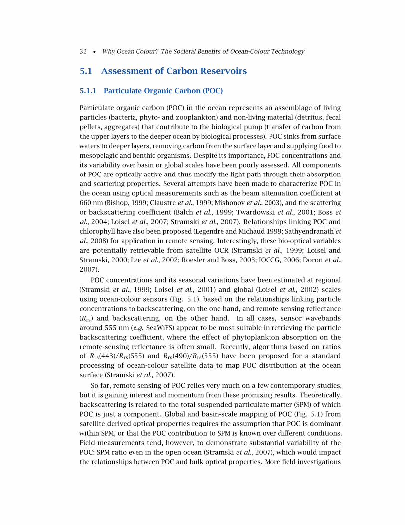
32 • Why Ocean Colour? The Societal Benefits of Ocean-Colour Technology
5.1 Assessment of Carbon Reservoirs
5.1.1 Particulate Organic Carbon (POC)
Particulate organic carbon (POC) in the ocean represents an assemblage of living
particles (bacteria, phyto- and zooplankton) and non-living material (detritus, fecal
pellets, aggregates) that contribute to the biological pump (transfer of carbon from
the upper layers to the deeper ocean by biological processes). POC sinks from surface
waters to deeper layers, removing carbon from the surface layer and supplying food to
mesopelagic and benthic organisms. Despite its importance, POC concentrations and
its variability over basin or global scales have been poorly assessed. All components
of POC are optically active and thus modify the light path through their absorption
and scattering properties. Several attempts have been made to characterize POC in
the ocean using optical measurements such as the beam attenuation coefficient at
660 nm (Bishop, 1999; Claustre et al., 1999; Mishonov et al., 2003), and the scattering
or backscattering coefficient (Balch et al., 1999; Twardowski et al., 2001; Boss et
al., 2004; Loisel et al., 2007; Stramski et al., 2007). Relationships linking POC and
chlorophyll have also been proposed (Legendre and Michaud 1999; Sathyendranath et
al., 2008) for application in remote sensing. Interestingly, these bio-optical variables
are potentially retrievable from satellite OCR (Stramski et al., 1999; Loisel and
Stramski, 2000; Lee et al., 2002; Roesler and Boss, 2003; IOCCG, 2006; Doron et al.,
2007).
POC concentrations and its seasonal variations have been estimated at regional
(Stramski et al., 1999; Loisel et al., 2001) and global (Loisel et al., 2002) scales
using ocean-colour sensors (Fig. 5.1), based on the relationships linking particle
concentrations to backscattering, on the one hand, and remote sensing reflectance
(Rrs) and backscattering, on the other hand. In all cases, sensor wavebands
around 555 nm (e.g. SeaWiFS) appear to be most suitable in retrieving the particle
backscattering coefficient, where the effect of phytoplankton absorption on the
remote-sensing reflectance is often small. Recently, algorithms based on ratios
of Rrs(443)/Rrs(555) and Rrs(490)/Rrs(555) have been proposed for a standard
processing of ocean-colour satellite data to map POC distribution at the ocean
surface (Stramski et al., 2007).
So far, remote sensing of POC relies very much on a few contemporary studies,
but it is gaining interest and momentum from these promising results. Theoretically,
backscattering is related to the total suspended particulate matter (SPM) of which
POC is just a component. Global and basin-scale mapping of POC (Fig. 5.1) from
satellite-derived optical properties requires the assumption that POC is dominant
within SPM, or that the POC contribution to SPM is known over different conditions.
Field measurements tend, however, to demonstrate substantial variability of the
POC: SPM ratio even in the open ocean (Stramski et al., 2007), which would impact
the relationships between POC and bulk optical properties. More field investigations
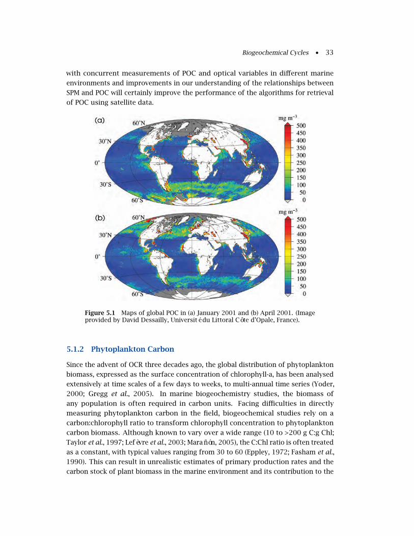
Biogeochemical Cycles • 33
with concurrent measurements of POC and optical variables in different marine
environments and improvements in our understanding of the relationships between
SPM and POC will certainly improve the performance of the algorithms for retrieval
of POC using satellite data.
Figure 5.1 Maps of global POC in (a) January 2001 and (b) April 2001. (Imageprovided by David Dessailly, Université du Littoral Côte d’Opale, France).
5.1.2 Phytoplankton Carbon
Since the advent of OCR three decades ago, the global distribution of phytoplankton
biomass, expressed as the surface concentration of chlorophyll-a, has been analysed
extensively at time scales of a few days to weeks, to multi-annual time series (Yoder,
2000; Gregg et al., 2005). In marine biogeochemistry studies, the biomass of
any population is often required in carbon units. Facing difficulties in directly
measuring phytoplankton carbon in the field, biogeochemical studies rely on a
carbon:chlorophyll ratio to transform chlorophyll concentration to phytoplankton
carbon biomass. Although known to vary over a wide range (10 to >200 g C:g Chl;
Taylor et al., 1997; Lefèvre et al., 2003; Marañón, 2005), the C:Chl ratio is often treated
as a constant, with typical values ranging from 30 to 60 (Eppley, 1972; Fasham et al.,
1990). This can result in unrealistic estimates of primary production rates and the
carbon stock of plant biomass in the marine environment and its contribution to the

34 • Why Ocean Colour? The Societal Benefits of Ocean-Colour Technology
global carbon budget (Faugeras et al., 2004). A more accurate assessment of this
factor could also lead to improved parameterisation of photosynthetic rates and
insights into physiological processes (e.g. growth rate).
The variability of the C:Chl ratio has been investigated primarily in laboratory
settings (Banse, 1977; Laws and Bannister, 1980; Geider, 1987; Geider et al., 1997).
It has been shown, experimentally, to be regulated by light level, temperature,
and nutrient availability (Geider, 1987; Cloern et al., 1995). The C:Chl ratio is
also tightly linked to phytoplankton growth (Landry and Hassett, 1982; Geider,
1987), and has been used in the calculation of the light-saturated photosynthetic
rate (Geider et al., 1998) and in the interpretation of widely used temperature-
growth relationships (Eppley, 1972). Under nutrient-replete conditions and at
balanced growth, C:Chl increases linearly with increasing irradiance levels (at constant
temperature), and decreases exponentially with increasing temperature (Geider,
1987). Nutrient limitation also impacts growth rate which translates into changes in
cellular C:Chl (Sakshaug et al., 1989).
Accordingly, empirical relationships have been established for C:Chl ratio as a
function of temperature, daily irradiance, and nutrient-limited growth rate (Cloern
et al., 1995). Their model includes both light-limited and nutrient-limited conditions.
Using this model and input variables from ocean-colour radiometry and other
satellite-derived data sets or atlases, it is possible to generate global fields of C:Chl
(Moore and Dowell, 2004). From another angle, Behrenfeld et al. (2005) provided
an initial attempt to map phytoplankton biomass in carbon units, and the C:Chl
ratio of phytoplankton on the global scale using the particulate backscattering
coefficient at 440 nm retrieved from OCR. The assumptions associated with this
study are more speculative than in the algorithms for retrieval of POC from space,
and must be carefully considered for any application of this method. More recently,
Sathyendranath et al., (2008) have used a large number of observations on POC and
chlorophyll, along with simple ecological considerations, to propose a method of
retrieving phytoplankton carbon from ocean colour. These recent investigations are
encouraging, and the knowledge of the phytoplankton C:Chl ratio from satellite data
may lead to improved calculations of the flow of carbon and energy through the
marine system and may also provide additional insight into the physiological status
of phytoplankton.
5.1.3 Particulate Inorganic Carbon (Calcium Carbonate)
Calcification is an integral component of the ocean carbon cycle and calcium
carbonate, whether in the form of calcite or aragonite, represents an important
constituent of the total marine particulate inorganic carbon (PIC). Calcification, as
described by the reaction:
Ca2+ + 2HCO−3 a CaCO3 +H2O + CO2, (5.1)
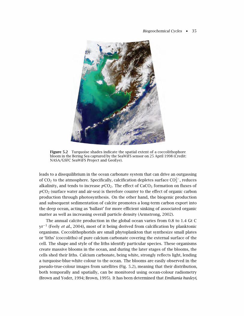
Biogeochemical Cycles • 35
Figure 5.2 Turquoise shades indicate the spatial extent of a coccolithophorebloom in the Bering Sea captured by the SeaWiFS sensor on 25 April 1998 (Credit:NASA/GSFC SeaWiFS Project and GeoEye).
leads to a disequilibrium in the ocean carbonate system that can drive an outgassing
of CO2 to the atmosphere. Specifically, calcification depletes surface CO2−3 , reduces
alkalinity, and tends to increase pCO2. The effect of CaCO3 formation on fluxes of
pCO2 (surface water and air-sea) is therefore counter to the effect of organic carbon
production through photosynthesis. On the other hand, the biogenic production
and subsequent sedimentation of calcite promotes a long-term carbon export into
the deep ocean, acting as ‘ballast’ for more efficient sinking of associated organic
matter as well as increasing overall particle density (Armstrong, 2002).
The annual calcite production in the global ocean varies from 0.8 to 1.4 Gt C
yr−1 (Feely et al., 2004), most of it being derived from calcification by planktonic
organisms. Coccolithophorids are small phytoplankton that synthesize small plates
or ‘liths’ (coccoliths) of pure calcium carbonate covering the external surface of the
cell. The shape and style of the liths identify particular species. These organisms
create massive blooms in the ocean, and during the later stages of the blooms, the
cells shed their liths. Calcium carbonate, being white, strongly reflects light, lending
a turquoise-blue-white colour to the ocean. The blooms are easily observed in the
pseudo-true-colour images from satellites (Fig. 5.2), meaning that their distribution,
both temporally and spatially, can be monitored using ocean-colour radiometry
(Brown and Yoder, 1994; Brown, 1995). It has been determined that Emiliania huxleyi,
36 • Why Ocean Colour? The Societal Benefits of Ocean-Colour Technology
a well-known and abundant coccolithophore, has increased its geographic range,
blooming with greater frequency in northern waters, such as the Bering Sea (Iida et
al., 2002) and the Barents Sea (Smyth et al., 2004a).
More importantly, specific algorithms have been elaborated to retrieve quantita-
tively calcite concentration and PIC standing stocks at regional and global scales (Fig.
5.3) from ocean-colour data (Gordon et al., 2001; Balch et al., 2005). An averaged,
global total of euphotic PIC, derived from MODIS data, has been estimated at 18.8
Mt, with systematically higher concentrations at latitudes greater than 30◦ (Balch et
al., 2005). It is possible that these values may be contaminated by other suspended
mineral compounds, e.g. opal from diatom populations (Broerse et al., 2003). More
verification with field measurements of PIC concentrations, PIC turnover time, and the
opal:PIC ratio are therefore necessary to optimize the use of ocean-colour radiometry
in models of the marine carbonate cycle.
Figure 5.3 Global composite images of seasonal suspended particulateinorganic carbon (PIC) concentration in 2002, as derived from MODIS/Terradata using a two-band calcite algorithm (adapted from Balch et al., 2005).
With increasing concern about marine acidification, it is not clear if coccol-
ithophores and other carbonate-dependant organisms can survive or adapt to a
high CO2 world. Substitution by other species will modify the overall ecosystem, as
well as the carbon budget in unknown ways. Long time-series of coccolithophore
blooms and PIC concentrations will be essential in studies on the impact of ocean
acidification on the marine ecosystem.

Biogeochemical Cycles • 37
5.1.4 Coloured Dissolved Organic Matter
One of the largest reservoirs of carbon on Earth is the organic matter dissolved
in the ocean (see review by Hansell and Carlson, 2002). The distribution, sources
and sinks of dissolved organic matter (DOM) in the ocean remains insufficiently
known. Obstacles to progress include the fact that DOM comprises a complex array
of molecules that are difficult to analyze and identify chemically. In practice, DOM
is defined operationally as the fraction of suspended material that goes through a
sub-micrometre filter (usually 0.2 µm). A fraction of DOM strongly absorbs light in
the UV-blue region of the spectrum, such that its presence turns the water yellow.
This is why it was originally called ‘gelbstoff’ or ‘yellow substance’ by oceanographers.
The term in common usage today for this component of DOM is chromophoric (or
coloured) dissolved organic matter, or CDOM. Its abundance in sea water can be
assessed through its optical properties, particularly the absorption coefficient at
blue wavelengths (Bricaud et al., 1981; Blough and Del Vecchio, 2002, and references
therein; Twardowski et al., 2004) which can be retrieved from space by ocean-colour
radiometry (Carder et al., 1999; Lee et al., 2002; Maritorena et al., 2002; Fichot et
al., 2008). However, the similarity between the absorption spectra of CDOM and
detrital matter, which decrease exponentially with wavelength, makes it impossible
to distinguish between the two using remote sensing. The retrieved absorption
coefficient is thus representative of some ‘coloured detrital material’ (CDM) combining
CDOM and detritus (IOCCG, 2006). Assuming a negligible contribution of detritus in
the open ocean, the global distribution of CDOM has been derived from ocean-colour
radiometry (Siegel et al., 2002; 2005). Obviously, the interpretation of these data
becomes more difficult in coastal waters where the contribution of organic detrital
matter could be significant. Most remote sensing algorithms treat the absorption
coefficient of CDM as a measure of its concentration. To convert absorption into
carbon units remains problematic. It is also not easy to establish the relationship
between the total detrital material and the coloured component.
In general, CDOM concentrations are higher in coastal areas compared with the
open ocean, pointing towards river and coastal runoff as being a major source of
CDOM in these areas. The source of CDOM in open ocean waters needs an improved
characterization (Nelson and Siegel, 2002), although its occurrence following bloom
peaks suggests a local origin from decaying phytoplankton cells, zooplankton grazing,
and microbial activity (Hu et al., 2006). In any case, CDM is an important element
in determining the light field in marine waters, which is required in the analysis of
photobiological and photochemical processes. CDOM has an important role in the
production of dissolved inorganic carbon (see section 5.2.2). Moreover, the variability
in CDM concentration affects the penetration of harmful UV radiation within the
surface layer with consequences for the surrounding ecosystem and biogeochemical
cycles. Finally, CDM can also be used as a tracer of water masses, particularly
freshwater inputs. CDM and salinity have often been found to vary inversely as river

38 • Why Ocean Colour? The Societal Benefits of Ocean-Colour Technology
water mixes with ocean water; thus, CDM can help to understand the interactions
between rivers and the coastal ocean (Ferrari and Dowell, 1998; Chen et al., 2007a).
Systematic observations of CDM over regional and basin scales using ocean-colour
radiometry are essential to gain a better understanding of the biogeochemical cycles
and to reduce uncertainties in the marine carbon cycle.
5.2 Carbon Fluxes
5.2.1 Calculating Phytoplankton Productivity from Ocean Colour
Ocean colour from satellite sensors offers the possibility of providing global
estimates of the most important transformation occurring in the ocean carbon
cycle: the conversion of inorganic carbon to organic carbon through photosynthesis,
termed primary production. This marine component of carbon fixation represents
approximately half the global total, making it a critical element of the Earth’s carbon
budget and biogeochemical cycles (Longhurst et al. 1995; Antoine et al., 1996;
Falkowski et al., 1998). Moreover, synoptic estimates of algal biomass and primary
production, as descriptors of the first trophic level, provide insights into the dynamics
of marine ecosystems. Access to estimates of primary productivity at spatial scales
of about one kilometre, and at time scales of about one week (average time required
to obtain clear skies for satellite observations) has thus become a considerable asset
in ocean sciences (e.g., Platt and Sathyendranath, 1988).
Primary productivity, P , at any particular location, depth (z), and time (t) in the
ocean is determined by chlorophyll-a concentration B(z, t) and a function (f(E))which describes the photosynthetic response of phytoplankton to the available
irradiance E(z, t), as follows:
P(z, t) = B(z, t)× f(E;z, t). (5.2)
In Equation 5.2, chlorophyll-a concentration is used as an index of phytoplankton
biomass, since it is the main data product derived from ocean-colour remote sensing,
and is also at the heart of the photosynthetic process. Another possibility is to use
phytoplankton carbon, but these methods require further research and validation as
mentioned previously. The irradiance, E, refers to that part of the electro-magnetic
spectrum between 400 and 700 nm, i.e., the photosynthetically available radiation
(PAR), expressed as a spectrally-resolved or integrated quantity. Surface PAR can
be derived directly from satellite ocean-colour radiometry (Frouin et al., 2003), or
using various spectral approaches based on remote sensing (Frouin and Pinker, 1995;
Bouvet et al., 2002). Other relevant environmental variables such as SST (which
appear in some implementations of the function f ) are also available from remote
sensing. Thus, in principle, we can retrieve the major elements required to calculate
primary productivity from satellite data.

Biogeochemical Cycles • 39
In reality, satellite ocean-colour radiometry is only sensitive to constituents in the
ocean upper layer, whereas biological and chemical processes such as photosynthesis
extend to deeper zones (e.g. 1% or 0.1% surface light level). The application of
Equation 5.2 therefore requires additional knowledge on the vertical structure of
the phytoplankton biomass (Platt et al., 1988; Morel and Berthon, 1989), and the
attenuation of irradiance with depth (Sathyendranath and Platt, 1989). Integration
of Equation 5.2 over depth and day-length provides an aerial daily rate of primary
production. Primary-production models may vary from each other depending on how
E is expressed (spectral or non-spectral), on how vertical structure of phytoplankton
is specified and on how the function f(E;z, t) in Equation 5.2 is specified (Platt et al.,
1977; Platt and Sathyendranath, 1993; Sathyendranath and Platt 1993; Behrenfeld
and Falkowski, 1997a; Sathyendranath and Platt 2007). Spectral models account for
the wavelength-dependent characteristics of the propagation and absorption of light,
whereas non-spectral models use total PAR. Time-integrated models express the
daily integrated productivity from daily averaged inputs. Depth-integrated versions
of models are also in use. Figure 5.4 shows an example of global primary production
calculated using a wavelength and depth-resolved primary production model.
Figure 5.4 Global primary production computed using MODIS-Aqua data fromJuly 2002 to June 2005 with a wavelength, depth-resolved, primary productionmodel down to the 0.1% light-level. (Credit: Frédéric Mélin, Joint ResearchCentre, EC, unpublished data. MODIS data provided by NASA/GSFC).
Regardless of the complexity of the model formulation, a critical aspect
of estimating productivity is specifying the photosynthetic parameters that are
contained in the term f in Equation 5.2. In particular, we need to know the rate
of photosynthesis per unit B, a property sometimes known as the photosynthetic
index, PB . The relationship between PB and E, the photosynthesis-irradiance (P − E)
curve, is well known empirically and can be described using two parameters: the

40 • Why Ocean Colour? The Societal Benefits of Ocean-Colour Technology
slope of the curve at the origin, and the maximum photosynthetic rate at saturating
light levels. As for the shape of the vertical biomass profile, this information is not
accessible directly from space, although PB at saturating light levels has been shown
to vary with temperature (Eppley 1972; Bouman et al. 2005), a relationship at the
heart of some models of productivity based on satellite data (e.g., Antoine et al.,
1996; Behrenfeld and Falkowski, 1997b). Another approach has been to identify
biogeochemical provinces for which a comprehensive data set of field measurements
enables the definition of representative photosynthetic parameters (Longhurst et
al., 1995; Sathyendranath et al., 1995). This method acknowledges the existence of
oceanographic regions characterized by distinct physical forcing and variability, as
well as the primary importance of the physical forcing in regulating algal processes
(Longhurst, 2006). Both implementation methods can be combined in various ways.
In any case, satisfactory representation of algal physiology at the global scale by
simple relationships applicable to remote sensing has so far proved elusive, though
regional approaches are promising (Bouman et al., 2005).
Several years ago, NASA established the Primary Productivity Working Group
(PPWG) to investigate the various issues surrounding the calculation of productivity
from ocean-colour radiometry. Campbell et al. (2002) reported the first results of a
comparison between different models using a database of in situ primary production.
The model results were generally within a factor of two of the observations. A similar
exercise conducted more recently by the PPWG (Carr et al., 2006) showed that most
models yielded an annual global primary production estimate in the range 35-60 Gt
C y−1. Breaking down the results by season or region can lead to larger differences
between the models. In the description of the approaches adopted for deriving
primary productivity from ocean-colour data, some of the assumptions, limitations
and difficulties have already been highlighted (Platt et al., 1988; Platt et al., 1995).
The discrepancies between satellite-derived products and field observations may be
grouped into the following sources of uncertainties: (1) the input fields from ocean
colour, mainly the surface concentration of Chl-a or the phytoplankton absorption
coefficient, and the optical properties of the other constituents, (2) the explicit or
implicit definition of a vertical structure for the algal biomass and the inherent
optical properties, (3) the propagation of the light field, and (4) the rate at which the
photons absorbed by the phytoplankton are used for photosynthesis.
The immense value of primary production estimates based on ocean-colour
radiometry and other remote-sensing data products is unquestionable. The
limitations noted above call our attention to the fundamental aspects of the
functioning of marine ecosystems and the challenges in their faithful representation
in models. Primary production models are continuously improving, owing to
advanced characteristics of on-going ocean-colour sensors, and significant progress
in bio-optical algorithms. A third exercise of the PPWG (Friedrichs et al., 2008)
demonstrated a reduction by 58% of the differences between ocean-colour derived
primary production and in situ data when compared with the first series of round-
Biogeochemical Cycles • 41
robin experiments by the PPWG to evaluate and compare primary productivity
algorithms. Another conclusion from this exercise is that algorithm performance is
not always related to model complexity (Campbell et al., 2002; Friedrichs et al., 2008).
This is not surprising considering the comprehensive knowledge on physiology
and optics required by all algorithms. However, the continuing development of
more elaborate, wavelength-resolved and depth-resolved models have the potential
to create new parameterizations and to provide better quality estimates as new
insights of the various processes involved are ascertained. At present, the greatest
uncertainty in production estimates arises from uncertainty in the estimate of Chl-a
from satellite data (Platt et al. 1995). As improved ocean-colour sensors lead to
better estimates of Chl-a and other bio-optical properties, one anticipates immediate
improvements in primary production estimates as well.
5.2.2 Photochemistry in the Upper Ocean
Both biogeochemistry of marine dissolved organic matter (DOM) and photochemistry
have shown impressive developments in recent years (Hansell and Carlson, 2002).
Deciphering the complex interactions of DOM with microorganisms and the radiation
regime is important in understanding the oceanic system and its relation with climate,
and the fate of terrestrial input of DOM into the oceans. As stated previously, the
absorption of coloured dissolved organic matter (CDOM) increases exponentially
towards the blue and ultraviolet wavelengths, a spectral domain that is very energetic
for photochemical reactions. The CDOM absorption of blue and UV light modifies
chemical species to more reactive forms (free radicals, other reactive species), that will
then take part in biochemical processes. The availability of CDOM absorption maps
from ocean colour (see section 5.1.4) thus opens new perspectives for quantifying
a complex array of biogeochemical rates. Some parallels can be made between
the framework of primary production modelling and photochemistry through the
definition of absorbed photochemically usable radiation, and quantum yield or action
spectra of photochemically-driven rates.
The direct production (through photo-oxidation) of carbon monoxide (CO) and
dissolved inorganic carbon (DIC) from terrestrial organic matter may be a major
term in the cycle of organic carbon (Miller and Zepp, 1995). The photochemical
degradation of DOM may also lead to eventual remineralisation of nitrogen-rich,
biologically available compounds (Bushaw et al., 1996). A major decomposition
process of the terrestrial inputs of DOM is the transformation into lower-molecular-
weight, more biologically-labile, organic substances. Various studies have shown how
this pathway modifies the availability of substrates for the microbial loop (Mopper
and Kieber, 2002). Photobleaching, the loss of colour and fluorescence properties due
to the degradation of chromophores induced by radiation, is a ‘visible’ manifestation
of these phenomena. This process has been well documented, particularly for coastal
waters. Far from land, the dynamics of CDOM is heavily conditioned by bleaching,

42 • Why Ocean Colour? The Societal Benefits of Ocean-Colour Technology
especially in the top layer of the water column (Nelson et al., 1998). Quantum yields
have been documented for photochemical production of DIC (Johannessen and
Miller, 2001), CO (Zafiriou et al., 2003), hydrogen peroxide (H2O2, Yocis et al., 2000),
biologically labile photoproducts (Miller et al., 2002) and CDOM photobleaching
(Del Vecchio and Blough, 2002). Global estimates of CO photoproduction using
SeaWiFS data have been presented by Miller and Fichot (2004). Organic compounds
and photochemical reactions are also part of the marine cycle of trace metals (e.g.,
Barbeau et al. 2001), important for phytoplankton populations.
Photochemical processes are also important drivers of the oceanic sulfur cycle
and DOM is an element of many of the related transformations. For instance in
the upper ocean, DOM is involved in the production (by photolysis) of carbonyl
sulfide, an important gas for stratospheric processes (Weiss et al., 1995). A similar
involvement of DOM also appears for the photolysis of dimethyl sulfide (DMS, e.g.,
Toole et al., 2003), a cycle that has received particular attention since the description
of possible climate feedbacks (Charlson et al., 1987). Also relevant to ocean-colour
radiometry is the use of Chl-a maps in association with physical variables to derive
surface concentrations of DMS at the global scale through empirical relationships
(Simó and Dachs, 2002).
That short-wavelength radiation is efficient for photosensitizing dissolved organic
compounds, and thus enhancing the overall reactivity of the medium, opens the door
to all sorts of processes and it is clear that many of those mentioned above interact.
For instance, photodegradation of DOM and microbial activity are intertwined.
Photobleaching of CDOM deepens the euphotic zone, and results in increased PAR in
the water, as well as increased potentially damaging, UV radiation. From the point of
view of carbon fluxes, photosynthesis is enhanced by a greater availability of light and
of macro- and micro-nutrients, whereas photochemical production of DIC reinforces
the source terms of CO2. Therefore, these various processes should be analyzed in
an integrated way. The extrapolation of local measurements to regional and global
scales will certainly require a better understanding of the complex photochemical
pathways. Ocean colour has an emerging role to play, by providing information on
the distribution of optically significant constituents, thus contributing to a better
definition of the light field in the ocean, but also more specifically to an assessment
of the CDOM dynamics.
5.3 Ocean Colour and Nitrogen Cycling
Total primary production in the ocean is partitioned into recycled production, which
is dependent on recycled nutrients in the upper layer, usually ammonia, and new
production, which is fuelled by allochtonous nitrogen supply (Dugdale and Goering,
1967). The paradigm in biological oceanography is that the vertical upwelling of
nitrate from the deep drives new production in the nutrient-limited regions of the

Biogeochemical Cycles • 43
surface ocean (Lewis et al., 1986). This process is well documented, particularly
in the equatorial ocean where surface chlorophyll increases with shoaling of the
thermocline, bringing more nutrients to the surface (Chavez et al., 1998; Siegel et al.,
1999; Ryan et al., 2002; Wilson, 2003). Nitrate is assumed to be the limiting nutrient
on short time scales (Lewis et al., 1986), outside of high-nutrient, low-chlorophyll
(HNLC) regions, where iron becomes a factor. Since transport of nitrogen from the
deep, cool waters to the surface is typically accompanied by a decrease in surface
temperature, it has been possible to use sea-surface temperature data to track the
supply of new nitrogen into the surface waters, and to use a combination of ocean-
colour and thermal infra-red remote sensing to measure new production in the
ocean (Dugdale et al., 1989; Sathyendranath et al., 1991; Goes et al., 2000). Campbell
and Aarup (1992) used information on the nitrate concentrations in oceanic waters
prior to the spring bloom, and mixed-layer depths at the time of the collapse of the
bloom, to derive consumption of nitrate by new production. In this study, CZCS data
were used to estimate the time of collapse of the blooms. Since only new nitrogen
can be responsible for phytoplankton growth in nitrogen- limited areas, primary
production integrated over the spring bloom can be used to infer a lower limit on
new production over that time interval (Platt and Sathyendranath, 2008).
Figure 5.5 Photograph of a Trichodesmium erythraeum bloom in the NorthEast Arabian Sea (off the Gulf of Khambhat), taken from the research vessel"ORV Sagar Kanya", April 2000. (Credit: Image provided by Shailesh Nayak,Space Applications Centre, ISRO, India).
Nitrogen fixation is another mechanism responsible for new production in the
ocean. Diazotrophs, organisms that fix nitrogen gas, can thrive in nitrate-depleted
waters, and might even shift the ocean from nitrogen to phosphorus limitation (Karl
et al., 1997; Cullen, 1999; Tyrrell, 1999). The most well-known oceanic diazotroph
is Trichodesmium (Fig. 5.5) but nitrogen fixation occurs in a number of organisms,

44 • Why Ocean Colour? The Societal Benefits of Ocean-Colour Technology
including unicellular cyanobacteria (Zehr et al., 2001; Montoya et al., 2004), and the
endosymbiotic Richelia that is found within several species of diatoms (Venrick,
1974; Villareal, 1992).
Recent studies have shown that nitrogen gas assimilated by nitrogen fixation
could form a significant proportion of the total oceanic new production (the fraction
of total primary production fuelled by nitrate) (Michaels et al., 1996; Karl et al., 1997;
Zehr et al., 2001). This source of new production could have an important impact
on the overall global carbon cycle since, unlike nitrate brought to the surface from
upwelling, N2-fixation is not coupled to fluxes of dissolved carbon from the deep
ocean, and can potentially drive a net uptake of atmospheric CO2 and export of
carbon (Hood et al., 2000). Another biologically mediated process that increases
surface nitrate is the vertical migration of Rhizosolenia diatom mats. These mats
use carbohydrate ballasting to migrate vertically between the nutricline, where they
uptake nitrate, and the surface, where they photosynthesize (Villareal and Carpenter,
1989; Villareal et al., 1999). Similar to nitrogen fixation, this process results in new
production without a flux of deep carbon to the surface, and so can result in more
efficient removal of carbon from surface waters (Richardson et al., 1998).
However, it remains difficult to quantify these processes because ship-based
observations can provide only limited coverage over large spatial scales. The high
spatial and temporal coverage of satellite chlorophyll data supports improved
assessments of these processes at regional and global scales. Two different
methodologies have been used to identify nitrogen fixation from ocean-colour data.
Genera-specific optical properties have been used to develop an algorithm to identify
Trichodesmium from analysis of satellite measured water-leaving radiances. Initial
algorithms only worked on significantly dense blooms, with chlorophyll values >1
mg m−3 (Subramaniam et al., 1999, Subramaniam et al., 2002), and therefore could
not be applied globally, as chlorophyll levels do not approach this threshold in
the oligotrophic ocean, where nitrate-deplete waters will favour nitrogen fixation.
Recently, a new algorithm has been developed that appears promising for detecting
Trichodesmium globally (Westberry et al., 2005). Such algorithms, however, are
genera specific, and will not identify production stimulated by other forms of
nitrogen fixation, or by migrating mats.
An alternative approach to identifying nitrogen fixation from satellite data takes
into account the oceanic conditions conducive to nitrogen fixation (and mat migration)
that are very different from conditions leading to upwelling-derived production.
Populations of Trichodesmium and Rhizosolenia mats are generally found in stable,
stratified waters, with low winds (Capone et al., 1997; Villareal and Carpenter, 1989;
Subramaniam et al., 2002). Trichodesmium is usually not present in waters colder
than 20◦C, and rarely blooms below 25◦C (Carpenter and Capone, 1992; Capone et
al., 1997; Subramaniam et al., 2002). Culture studies indicate an ideal temperature
range of 24 to 30◦C for Trichodesmium (Breitbarth et al., 2007).
Chlorophyll blooms in the southwest Pacific, observed by both CZCS and SeaWiFS,

Biogeochemical Cycles • 45
Figure 5.6 Monthly SeaWiFS composite of chlorophyll for October 2000,showing a large chlorophyll bloom northeast of Hawaii in the oligotrophicPacific. The bloom developed at the end of August and lasted into December. Ithas been speculated that the bloom was driven by nitrogen fixation or verticallymigrating diatom mats (adapted from Wilson, 2003).
have been identified as Trichodesmium, based on previous reports of Trichodesmium
in the area, especially in summer when the surface water is warm and stratified
(Dupouyet al., 1988; Dupouy et al., 2000). Chlorophyll blooms which develop in late
summer in the oligotrophic Pacific, northeast of Hawaii, have been observed by CZCS,
OCTS and SeaWiFS, as seen in Figure 5.6 (Wilson, 2003; Wilson et al. 2008). The
cause of these blooms has been attributed to either nitrogen fixation (although not
necessarily Trichodesmium) or vertically migrating Rhizosolenia diatom mats, based
on concurrent SSH and SST data, and previous biological observations in the area
(Wilson, 2003; Wilson et al., 2008). Since diatom blooms are important mechanisms
for sequestering carbon into the deep ocean (Goldman, 1988), the carbon export from
these blooms could be significant given their size and duration: they can become
as large as the state of California and can last up to 5 months. A similar analysis
of satellite data (Coles et al., 2004) has identified an annual summer chlorophyll
bloom in the western tropical Atlantic as attributable to nitrogen fixation. Coles et
al. (2004) showed further that the seasonal cycle of satellite chlorophyll for this area
could only be reproduced in a biological model that explicitly simulated nitrogen
fixation.
The approach of using multiple satellite measurements to identify production
under conditions favouring diazotrophy (stratified, low nutrient, high light, sufficient
iron) can provide a means for estimating patterns of nitrogen fixation on global scales.
If diazotrophs have the potential to shift the ocean from nitrogen to phosphorus
limitation (Karl et al. , 1997) and alter global climate through changes in the biological
pump (Michaels et al., 2001; Sañudo-Wilhelmy et al., 2001), then improving our
understanding of their spatial and temporal patterns and production is essential.

46 • Why Ocean Colour? The Societal Benefits of Ocean-Colour Technology
5.4 Future Directions
Optical remote sensing aims at quantifying optical properties in the surface layer of
the oceans. Algorithms have been steadily increasing and diversifying in the remote-
sensing era. Nevertheless, there is a demand for even better descriptions of marine
absorption and scattering properties, especially those associated with phytoplankton
stocks or CDOM absorption. This is particularly true in coastal waters, which are also
areas of intense biogeochemical cycling. In turn, better optical descriptions may lead
to more accurate derived information on dissolved and particulate organic carbon
or particle size spectra that can be used in studies of biogeochemistry. Also, the
detection of phytoplankton functional groups has been proposed by Sathyendranath
et al. (2004), Alvain et al. (2005) and Aiken et al. (2008) among others, and such
techniques would favour a better representation of algal physiology in satellite-based
models of primary production.
Moreover, an improved retrieval of optical properties will improve the modelling
of radiative transfer in the water column. The importance of an accurate, spectral,
three-dimensional depiction of the light field in the ocean cannot be understated
for studies of biogeochemical cycles, because of its effects on physics, biology and
chemistry. Clearly, the potential of ocean colour in the field of biogeochemistry
will be enhanced if links between other remote-sensing products and dynamic
models are improved. Besides accurate bio-optical measurements, applications
of ocean colour to biogeochemical cycles will benefit from data sets gathered by
field measurements. For example, the progress of Fast Repetition Rate Fluorometer
(FRRF)-based techniques to determine in situ primary productivity or photosynthetic
parameters (e.g. Smyth et al., 2004b) will help primary production modelling, while
autonomous sensors (Bishop et al., 2002) will complement studies of particles and
carbon dynamics in the ocean. Finally, understanding biogeochemical cycles relies on
long-term data series, and the existence of an ocean-colour record that now exceeds
10 years will give more weight to studies addressing time scales beyond the seasonal
cycle.

Chapter 6
Ocean-Colour Radiometry and Fisheries
Cara Wilson, Jesus Morales, Shailesh Nayak, Ichio Asanuma andGene Feldman
The food requirements of an expanding human population have increased the
pressure on fisheries resources. In the last half century the world fish harvest has
increased more than four-fold from 20 million tonnes in 1950 to 95 million tons
in 2004 (FAO Fisheries Department, 2007). However, the number of overexploited
or depleted stocks has increased, and the capture fishery production has, in fact,
declined or remained static since 2000, reflecting over-harvest in many regions
(Hilborn et al., 2003). Better fisheries management, through a deeper understanding
of marine ecology, is needed to maximize the utility of living marine resources
now and into the future. A major challenge for fisheries scientists is distinguishing
fluctuations caused by human activities (such as overexploitation, habitat alteration
and pollution) from natural environmental variability. Over 100 years ago with the
formation of the International Council for the Exploration of the Seas (ICES), the
fundamental question of what drives the interannual variability of fish stocks was
first posed, and still has not been adequately resolved (Kendall and Duker, 1998;
Bakun and Broad, 2003; Anderson et al., 2008).
In the broadest sense, fisheries science encompasses not just commercial fish
stocks, but all living marine resources, including efforts to help recover threatened
and endangered species. Satellite data can be used to characterize the habitat
and ecosystem properties that influence marine resources at large temporal and
spatial scales, and high temporal and spatial resolution. There are two primary ways
that ocean-colour data are used for fisheries management. One is to monitor the
environment, with a view to better understand ecosystem processes or stock biology.
The other is to locate populations of fish, with a view to increase fishing efficiency or
enhance conservation by mitigating human interactions. Additionally, ocean-colour
data are used to monitor a number of issues that impact fisheries, such as harmful
algal blooms and coastal pollution, which are discussed in further detail elsewhere
in this volume.
47

48 • Why Ocean Colour? The Societal Benefits of Ocean-Colour Technology
6.1 The Oceanic Food Web
Satellite chlorophyll provides an index of phytoplankton biomass, which is the base
of the oceanic food web, as depicted in simplified form in Figure 6.1. The relationship
between satellite chlorophyll data and a specific fish stock depends upon the number
of linkages between phytoplankton and the higher trophic level. For some species,
such as anchovies and sardines, which eat phytoplankton at some points in their life
cycle, the linkage can be direct (Ware and Thomson, 2005), whereas for other species
there are many trophic levels in between, and the relationship can be quite non-linear.
There can also be spatial disconnects between satellite measurements of the ocean
surface and demersal and deep-water species. Nonetheless, chlorophyll is the only
Figure 6.1 Simplified oceanic food web, showing the varying complexities inthe linkages between phytoplankton, measured by satellite ocean-colour data,and higher trophic levels. Modified from Pauly and Christensen (1995).
biological component of the marine ecosystem accessible to remote sensing, and as
such it provides a key metric to measuring ecosystems on a global scale. Satellite
chlorophyll measurements are the primary component in algorithms to calculate the
primary productivity (PP) of the ocean. Global PP measurements, in conjunction with
fish catch statistics and food web models, such as shown in Figure 6.1 can be used
to estimate the carrying capacity of the world’s fisheries. In the open ocean 2% of
the PP is needed to support the fishery catch, but in coastal regions the requirement
ranges from 24-35%, suggesting that these systems are at or beyond their carrying
capacity (Pauly and Christensen, 1995), which is cause for concern as the bulk of
the world’s fish catch comes from coastal areas. In a similar manner, discrepancies
between the values of satellite derived PP and reported fish catches have been used
to demonstrate spurious trends in global fish catches as reported by the Food and
Ocean-Colour Radiometry and Fisheries • 49
Agriculture Organization (FAO) of the United Nations (Watson and Pauly, 2001). In
this instance satellite ocean-colour data provide an important objective baseline
against which to gauge data that can have socio-economic biases.
There is growing awareness that the long-standing approach to fisheries
management which focuses on a specific species is inadequate (Browman and
Stergiou, 2005; Sherman et al., 2005). Interactions with other species, complex
predator-prey dynamics, and temporal and spatial variability in physical aspects
of the ecosystem all need to be incorporated into an ecosystem-based approach to
management. Although not all of these aspects can be addressed by satellite data,
the high spatial and temporal resolution of satellite ocean-colour data make it an
efficient tool to characterize and monitor marine ecosystems to better manage them.
For example, satellite-derived primary productivity is one of the indicators used in
the assessment of Large Marine Ecosystems (LME) (Sherman et al., 2005).
6.2 Recruitment
A fundamental issue in fisheries oceanography is understanding how environmental
variability affects annual recruitment, the number of new individuals entering a
stock. Most fish have planktonic larval stages that are strongly influenced by ocean
circulation and can have narrow ranges of optimal thermal conditions. Availability
of a suitable food source is important for successful recruitment and hence many
fish reproduce near the seasonal peak in phytoplankton abundance. A long-standing
hypothesis in fisheries has been that recruitment success is related to the degree of
timing between spawning and the seasonal phytoplankton bloom, the Cushing-Hjort
or match-mismatch hypothesis (Cushing, 1990). This hypothesis has been difficult
to address with traditional shipboard measurements that have limited spatial and
temporal resolution, but with satellite ocean-colour data, interannual fluctuations in
the timing and extent of the seasonal bloom can be clearly seen. In an application
on the Nova Scotia Shelf, the timing of the spring bloom determined from satellite
ocean colour was compared with available in situ data on larval survival of haddock,
an important commercial fish species. Comparison of these two independent data
sets indicated that highly successful year classes of haddock are associated with
exceptionally early spring blooms of phytoplankton (Fig. 6.2), confirming the match-
mismatch hypothesis (Platt et al., 2003). A comparable study has also documented a
relationship between the timing of the spring bloom and the growth rate of shrimp
(Fuentes-Yaco, 2007). These studies demonstrate that it is possible to separate
ecosystem-associated variability in fish stocks from other components, such as
human exploitation or predation effects. The satellite-derived time series permits
the extraction of value-added products, in this case the timing of the seasonal
biological cycle.

50 • Why Ocean Colour? The Societal Benefits of Ocean-Colour Technology
Figure 6.2 (a) Timing of the maximum phytoplankton biomass in the NWAtlantic from February to July, derived from SeaWiFS climatology (1998-2001).Units in weeks; blue indicates early spring bloom (March), red indicateslate spring bloom (July). Image provided by César Fuentes-Yaco, DalhousieUniversity, Canada. (b) Relationship between larval haddock survival index(normalized to recruitment) and local anomalies in bloom timing. Data from thecontinental shelf off Nova Scotia (see black rectangle on map) for the periods1979-1981 and 1997-2001, adapted from Platt et al. (2003).
6.3 Harvesting
Locating and catching fish is becoming more challenging as easily accessible fish
stocks dwindle. As search time increases, so does cost. Satellite data can help to
increase the efficiency of fishing efforts by identifying oceanographic features that
are sites of fish aggregation and migration such as temperature fronts, meanders,
eddies, rings and upwelling areas (Laurs et al., 1984; Fiedler and Bernard, 1987;
Chen et al., 2005). Fishermen have been using SST from the Advanced Very High
Resolution Radiometer (AVHRR) on the NOAA polar orbiting satellite for the past
20 years. Fishermen also use remotely-sensed ocean-colour maps at sea to guide
fishing effort. Thermal or colour gradients often indicate sites of high biological
productivity. Temperature is also an important factor determining the distribution
of fish, as different species have different preferred temperature ranges.
To be of practical use to the fishing industry, satellite ocean-colour data must be
available in a near-real time basis. There are differences between countries in how
satellite data is disseminated to users. While in some countries, notably Japan and
India, the national fisheries agencies are actively involved with helping to increase
the efficiency of their fishing fleets. NOAA Fisheries in the USA is not allowed to

Ocean-Colour Radiometry and Fisheries • 51
provide services such as distributing ‘fish finding maps’ that would compete with
commercial interests. For example, the SeaWiFS satellite is privately owned, and its
chlorophyll data is only available on a real-time basis to commercial subscribers.
Clients of the service company can receive custom-tailored maps of ocean colour,
as well as other oceanic properties derived from satellite data, directly onboard
their fishing vessel. In contrast, data from the Indian IRS-P4 ocean-colour sensor (in
conjunction with satellite SST from AVHRR) is used operationally to produce maps
of potential fishing zones (PFZs).
6.3.1 Potential Fishing Zones: The Indian Experience
Methods for locating potential fishing zones (PFZ) in India from satellite data were
developed initially through detection of SST gradients revealed by oceanic features
such as fronts, eddies and upwelling (Lasker et al. 1981, Laurs et al. 1984, Narain
et al. 1990) known to be conducive to fish aggregation. This approach has the
Figure 6.3 Chlorophyll image of northwest India on 29 February 2006generated from the Indian OCM sensor. Oceanic features such as cycloniceddies (1 and 2 on the image) and fronts (3 and 4) are known to be productivesites and are hence relevant for fishery exploration (Credit: R.M. Dwivedi, IndianSpace Research Organisation, India).
basic limitation that SST images provide data on the temperature of the surface
skin only (upper ten microns). Heating of sea surface, particularly in equatorial
and tropical waters during summer, gives rise to strong stratification of the water
column, preventing arrival of cool nutrient rich waters from deeper layers to the
surface. This, in turn, inhibits appearance of SST gradients in the satellite imagery.
For this reason, SST images are not always adequate for identification of potential
fishing zones. Another problem with detection of thermal features is that surface

52 • Why Ocean Colour? The Societal Benefits of Ocean-Colour Technology
frontal structures may be perturbed by prevailing surface winds or currents of even
moderate magnitude (Dwivedi et al., 2005). Unlike thermal sensors, ocean-colour
Figure 6.4 An example of a chlorophyll map overlaid with SST contours, fordetection of Potential Fishing Zones (PFZ). The chlorophyll image was capturedby India’s IRS-P4 OCM sensor on 29 February 2000 off the west coast of India(Credit: Space Applications Centre, Indian Space Research Organisation, India.)
sensors can detect signals from below the surface due to penetration of visible
radiation down to one attenuation depth (typically metres to tens of metres), and
thus have advantages over the SST-based approach for fishery applications. One of
the benefits of water penetration capability of visible radiation is that it provides
the ability to predict occurrence of oceanic features such as diverging fronts and
eddies (Fig. 6.3). These features are known to be the most reliable indicators of
potential fishing zone (Laurs et al. 1984). It also enables detection of variations in
biomass in a column at different stages of feature development in serial chlorophyll
images. This advantage was exploited to develop the ability to anticipate formation
of oceanic features such as eddies, at least two days before their actual occurrence.
Verification of the experimental forecasts with inclusion of ocean colour proved
superior to those using SST alone in terms of rate of success and magnitude of fish
catch. Secondly, chlorophyll images, unlike those of SST, reveal many more frontal
structures, given the penetration capability of visible radiation. Moreover, unlike
SST, the ocean-colour front detected from chlorophyll image is a true biological front
and hence, relevant to exploration for fish.
Two approaches are routinely used by the Indian National Centre for Ocean
Information Services (INCOIS) to identify potential fishing zones. In the first approach,

Ocean-Colour Radiometry and Fisheries • 53
Figure 6.5 This image shows chlorophyll concentrations off the west coast ofIndia, captured by India’s OCM sensor onboard the Oceansat-1 satellite on 17November 1999 . Arrows indicate areas where fishing was conducted (Credit:Space Applications Centre, Indian Space Research Organisation, India).
SST contours derived from NOAA-AVHRR data are overlaid on chlorophyll images
generated from the Indian OCM sensor, to enable identification of matching features
revealed by corresponding gradients (Solanki et al. 2000) (Fig. 6.4). This method
has provided consistent positive feedback, although frontal structures common
in both SST and chlorophyll images are generally few in number. There are many
more features detectable from a chlorophyll image for which there is no matching
counterpart in SST images, so the second approach uses satellite chlorophyll data
alone, especially when relatively sparse thermal gradients are detected in SST imagery
(Fig. 6.5). Selective use of these additional features from ocean-colour imagery
has successfully enabled identification of potential fishing zones, and is a major
contribution to the improved fishery forecast in Indian waters. Nayak et al. (2003)
carried out a cost benefit analysis to assess the impact of using satellite PFZ forecasts
on fish catch. The benefit-to-cost ratio (i.e. value of the fish catch vs. cost of fishing
and generating PFZ charts) was found to be greater than one, indicating that the use
of satellite data improves the economics of fish catch.
Using the above approaches, INCOIS generates PFZ advisories three times a week,
providing information such as latitudes and longitudes of the areas of potential fish
abundance, and the distance and direction from different fishing harbours. This
information is freely disseminated to local fishermen around the coast of India by
fax, phone, internet, electronic display boards, newspaper and radio broadcasts in
local languages. In order to maintain fish stocks at a sustainable level, PFZ advisories
are not provided during the monsoon season (June-September), which coincides with

54 • Why Ocean Colour? The Societal Benefits of Ocean-Colour Technology
the peak breeding season, and also with heavy cloud cover. These advisories have
helped to reduce search time by up to 70%, and have significantly increased the catch
per unit effort (Solanki et al., 2003; Zainuddin et al., 2004). This is a prime example
of how satellite data can be put to effective use to ensure that the advantages of
science and technology directly benefit society.
6.3.2 Pelagic and Migratory Fish: A Japanese Case Study
In the northwest Pacific, Skipjack tuna, a pelagic and highly migratory fish, are
at the top of the pelagic food chain and support a valuable commercial fishery
(Iizuka et al., 1989; Shetty et al., 1993). Skipjack tuna migrate between the subarctic
(Oyashio) and the subtropical (Kuroshio) waters in the western Pacific (Kawasaki
and Omori, 1995; Watanabe et al., 1995), while planktivorous fish, such as Japanese
sardine, Chub mackerel and Pacific saury also migrate between the two regions
(Yasuda and Watanabe, 1994; Taniguchi, 1999). Satellite-borne sensors, such as the
Figure 6.6 Distribution of Chl-a concentrations for 23-29 September, 2000,observed by SeaWiFS, and Skipjack tuna catches by fishing boats (in tonnes).The size of the triangles indicates the landings (tonnes per day). Image providedby Ichio Asanuma, Tokyo University, Japan.
Japanese Ocean Colour Temperature Scanner (OCTS), have been used to monitor
the distribution of Chl-a with respect to the distribution of fish (Ishizaka, 1998;
Asanuma et al., 2003). In the northwest Pacific, complex mixing processes have been
observed between the warm, nutrient-depleted water from the Kuroshio and the cold,

Ocean-Colour Radiometry and Fisheries • 55
nutrient-rich water from the Oyashio (Saitoh et al., 1998). In general, the warmer
Kuroshio water has a low Chl-a concentration while the colder Oyashio water has a
high Chl-a concentration, with complex variability in regions of mixing (Yoshimori et
al., 1995; Ono et al., 1998).
Figure 6.7 Distribution of Skipjack tuna, Chub mackerel and Pacific saury asa function of Chl-a and SST. Chl-a was obtained from SeaWiFS data, while SSTwas derived from NOAA-AVHRR data. Average SST and Chl-a concentrationswere 21.0◦C and 0.46 mg m−3 for Skipjack tuna, 23.0◦C and 0.99 mg m−3 forChub mackerel, and 17.2◦C and 1.54 mg m−3 for Pacific saury. The study areaencompassed 35◦N to 45◦N and 140◦E to 150◦E over the period 23-29 September,2000. Image provided by Ichio Asanuma, Tokyo University, Japan.
In an experiment to assess the utility of providing Chl-a imagery to fishermen to
determine fishing grounds, the highest catches (> 30 tonnes) were reported between
two warm core rings around 41◦N and 145◦E (Fig. 6.6). Slightly lower catches (10 -
19 tonnes) were reported around 42◦N and 153◦E, along the boundary of the high
Chl-a Oyashio and the low Chl-a Kuroshio. Very low catches of Skipjack tuna (2 to 4
tonnes) were evident further east (around 156◦E) in the warmer, nutrient-depleted
waters. Planktivorous Pacific saury and Chub mackerel were caught in water masses
with high Chl-a concentrations (Fig. 6.7), although they tend to prefer different
temperature ranges, with a mean temperature of 17.2◦C and 23◦C respectively. In
contrast, Skipjack tuna catches occurred in a wide range of Chl-a concentrations (0.1
to 10 mg m−3) and in temperatures ranging from 18◦C to 25◦C. Nonetheless, the
majority of Skipjack tuna were caught in lower Chl-a waters (mean 0.46 mg m−3),
which corresponds to the warm core rings originating from the Kuroshio (mean
temperature 21.0◦C).

56 • Why Ocean Colour? The Societal Benefits of Ocean-Colour Technology
6.4 Species of Conservation Concern
6.4.1 Right Whales
One of the most endangered marine species is the Northern right whale (Eubalaena
glacialis), with an estimated population of 350 individuals (International Whaling
Commission, 1998; Kraus et al., 2005). Although historically right whale populations
were severely depleted by commercial whaling, at present the principal cause of
mortality in the North Atlantic is from ship strikes (National Marine Fisheries Service,
2005). The primary habitat of the North Atlantic right whale is in coastal or shelf
waters, which also experience heavy ship traffic. The recovery plan of NOAA (USA)
for this species has focused on developing methods to identify the locations of
right whale populations, and then to reduce ship traffic in these regions and lessen
the number of whale-vessel collisions. This plan involves both limiting fishing in
certain areas when whales are typically abundant, a procedure known as seasonal
area management (SAM), and another strategy known as dynamic area management
(DAM), with a synoptic level of control. Under DAM, if a group of whales is identified,
NOAA Fisheries will limit activities in the area. Currently, research is underway
to improve both management strategies by predicting the location of right whale
congregations using satellite measurements of SST and ocean colour (Pershing et al.,
2008). The distribution of right whales is strongly correlated with the distribution
of their prey, which appears to be primarily calanoid copepods (Kenney et al., 2001).
Satellite-derived chlorophyll data is a reasonable proxy for copepod egg production,
and is analyzed in conjunction with SST data to estimate the development time of
copepods, and model data to understand circulation patterns, to ultimately predict
areas where whale aggregation is likely. This project is moving from proof of concept
to operations, and daily Calanus distributions and right whale estimates should be
available shortly. The science team is working with NOAA Fisheries to incorporate
the products into right whale management.
6.4.2 Loggerhead Turtles
Satellite ocean-colour data, in conjunction with telemetry data from tagged sea
turtles have shown that in the North Pacific, the Transitional Zone Chlorophyll Front
(TZCF) is an important foraging ground and migration pathway for endangered
loggerhead turtles (Polovina et al., 2004). These turtles follow the TZCF, and spend
time foraging in the high chlorophyll eddies that are associated with meandering
of the front (Fig. 6.8). Other apex predators such as albacore tuna also use the
front as a migratory corridor (Laurs and Lynn, 1991; Polovina et al., 2001). The
degree of meandering of the TZCF seems to impact trophic transfers and the level of
productivity associated with the front. Periods with more meandering of the front
have had significantly higher catch per unit effort (CPUE) of albacore, suggesting
that the enhanced convergence creates more productive foraging grounds (Polovina
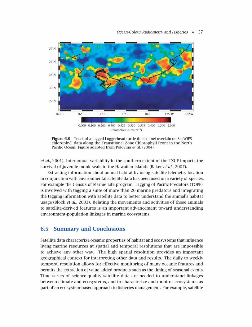
Ocean-Colour Radiometry and Fisheries • 57
Figure 6.8 Track of a tagged Loggerhead turtle (black line) overlain on SeaWiFSchlorophyll data along the Transitional Zone Chlorophyll Front in the NorthPacific Ocean. Figure adapted from Polovina et al. (2004).
et al., 2001). Interannual variability in the southern extent of the TZCF impacts the
survival of juvenile monk seals in the Hawaiian islands (Baker et al., 2007).
Extracting information about animal habitat by using satellite telemetry location
in conjunction with environmental satellite data has been used on a variety of species.
For example the Census of Marine Life program, Tagging of Pacific Predators (TOPP),
is involved with tagging a suite of more than 20 marine predators and integrating
the tagging information with satellite data to better understand the animal’s habitat
usage (Block et al., 2003). Relating the movements and activities of these animals
to satellite-derived features is an important advancement toward understanding
environment-population linkages in marine ecosystems.
6.5 Summary and Conclusions
Satellite data characterize oceanic properties of habitat and ecosystems that influence
living marine resources at spatial and temporal resolutions that are impossible
to achieve any other way. The high spatial resolution provides an important
geographical context for interpreting other data and results. The daily-to-weekly
temporal resolution allows for effective monitoring of many oceanic features and
permits the extraction of value-added products such as the timing of seasonal events.
Time series of science-quality satellite data are needed to understand linkages
between climate and ecosystems, and to characterize and monitor ecosystems as
part of an ecosystem-based approach to fisheries management. For example, satellite

58 • Why Ocean Colour? The Societal Benefits of Ocean-Colour Technology
chlorophyll can be used to observe changes in the timing of the spring bloom that
can affect recruitment (Platt et al., 2003), to classify the productivity of the oceans
(Sherman et al., 2005), to detect interannual differences in the frontal structures that
are important to fisheries (Bograd et al., 2004; Polovina et al., 2001) and to map the
spatial extent of the ocean experiencing lower productivity during an El Niño event
(Wilson and Adamec, 2001). Near-real-time satellite data are needed to optimize
sampling for fisheries survey cruises for management and stock assessment and
also to increase the efficiency of fishing effort.
Chapter 7
Ocean-Colour Radiometry and Water Quality
Nicolas Hoepffner, Christopher Brown, Roland Doerffer, Joji Ishizaka,Jim Gower and Mervyn Lynch
All water systems, such as inland surface waters, estuaries, coastal waters and ground-
waters, are exposed to increasing external pressures, resulting from climate change
and direct human activities. Pressures that are expected to have the largest impact
on water systems are temperature changes, sea-level rise, increasing greenhouse
gases in the atmosphere, and increasing precipitation and river runoff. In addition,
water bodies receive agricultural, domestic and industrial pollutants, and are subject
to recreational pressures from the leisure industry, as well as intensive fishing and
farming of marine organisms. These pressures are interconnected and may be
acting concurrently to reduce water quality and contribute to the deterioration of
the ecosystem, including habitat loss and reduced biodiversity.
To lessen or reverse negative trends, national plans and international programmes
have recently emerged to assess and monitor the present quality status of water
bodies. The Water Framework Directive in the EU (EC, 2000) sets the goal of achieving
a ‘good status’ for all of Europe’s surface waters by 2015. Similarly, Goal 2 of the
National 2006-2011 Strategic Plan in the US (US Environmental Protection Agency,
2006) targets a full recovery of water quality standards in more than 2,250 ‘polluted’
water bodies by 2012.
These plans establish reference conditions and reference sites for an inter-
calibration network, to specify indicators and criteria for an ecological status
classification system, and to implement appropriate measures that would sustain an
improvement of the aquatic environment.
7.1 Conceptual Framework for Satellite Water QualityMonitoring
Many chemical and biological characteristics are used, either individually or in
combination, as indices to assess water quality. Appropriate measurements and
thresholds are prescribed according to the targeted application of the water systems,
e.g., drinking water, bathing water, or water used in industry and aquaculture.
59

60 • Why Ocean Colour? The Societal Benefits of Ocean-Colour Technology
However, a common set of key water-quality indicators that include physical,
chemical, and biological endpoints such as conductivity, dissolved oxygen, pH,
turbidity, biomass concentration, total suspended matter, pathogens and primary
production, can be identified from various legislation texts and directives.
In coastal and marine waters, the variables associated with a defined ‘quality
status’ can change over a wide range of spatial and temporal scales, leading to
substantial logistic and economic difficulties to monitor them on a regular basis.
Realistically, the approach to coastal water management is to undertake ongoing
assessments of the population and condition of marine flora and fauna, as well
as what might be termed ‘water quality’. This approach usually employs in situ
techniques, which correspond essentially to a statistical/spatial sampling of the
system, and has been designed to capture the key attributes and system spatial
variability. It is important to recognize that these in situ efforts are extremely
valuable, though costly, and need to be implemented at regular intervals if they
are to become a meaningful management tool. However, an in situ approach can
rarely sustain the repeat frequency and spatial coverage that is required to support
effective management practices in vulnerable areas, where more intensive monitoring
needs to be in place. Processes such as coastal currents, sediment transport from
flooding river systems, wind driven vertical mixing, coastal upwelling, nutrient fluxes
and algal blooms can rapidly modify coastal water properties. It is likely that these
changes will not be captured by in situ sampling on an adequate spatial and temporal
scale. In contrast, satellite remote sensing is particularly good at depicting changes
in the water properties at appropriate scales. Over the past decade, several studies
have demonstrated the utility of satellite measurements of ‘water colour’ to assess
water quality (Prasad et al., 1998). Several of the indicators are directly or indirectly
related to the colour or reflectance of the water and, therefore, potentially accessible
from remote sensing.
The colour of a water body, as recorded by a satellite, depends on the capacity of
the water constituents to absorb and scatter solar radiation at specific wavelengths.
As the concentration and variety of the constituents increase in the water column,
the interpretation of ocean-colour data becomes more difficult. Often, turbid or
‘Case 2’ waters (Morel and Prieur et al., 1977; Sathyendranath et al., 1989), occur
in areas requiring specific attention with respect to water quality assessment. The
new generation of optical sensors, and new algorithms that have been developed
to specifically address the problem of differentiation between optically-active
components in Case 2 waters (IOCCG, 2000), provide a basis for an operational
cost-benefit analysis of water quality in sensitive and economically important areas.
A brief review of operational ocean-colour products that are currently available
or under development is presented in a previous IOCCG Report (IOCCG, 2000).
Several of these products can be used directly as water quality indicators. For
example, satellite estimates of the light attenuation at different wavelengths provide
information on the depth of penetration of the solar radiation and, therefore, can be
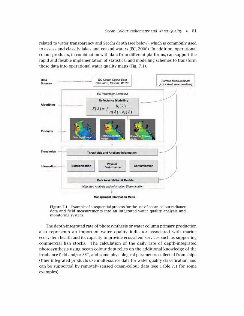
Ocean-Colour Radiometry and Water Quality • 61
related to water transparency and Secchi depth (see below), which is commonly used
to assess and classify lakes and coastal waters (EC, 2000). In addition, operational
colour products, in combination with data from different platforms, can support the
rapid and flexible implementation of statistical and modelling schemes to transform
these data into operational water quality maps (Fig. 7.1).
Figure 7.1 Example of a sequential process for the use of ocean-colour radiancedata and field measurements into an integrated water quality analysis andmonitoring system.
The depth-integrated rate of photosynthesis or water column primary production
also represents an important water quality indicator associated with marine
ecosystem health and its capacity to provide ecosystem services such as supporting
commercial fish stocks. The calculation of the daily rate of depth-integrated
photosynthesis using ocean-colour data relies on the additional knowledge of the
irradiance field and/or SST, and some physiological parameters collected from ships.
Other integrated products use multi-source data for water quality classification, and
can be supported by remotely-sensed ocean-colour data (see Table 7.1 for some
examples).

62 • Why Ocean Colour? The Societal Benefits of Ocean-Colour Technology
Table 7.1 Products or state indicators and their applications.
Product Name Standard and Advanced Product Application
Requirement
Transparency / Pigments, total suspended matter (TSM), Water quality monitoring
Secchi disk depth light attenuation coefficient, dissolved
organic matter (DOM),
Primary production Pigments, TSM, DOM, inherent optical Water quality monitoring,
properties of water constituents, SST, ecosystem and habitat
surface irradiance assessment
Differential biomass/ Pigments, chemotaxonomic equations Water quality monitoring,
phytoplankton ecosystem assessment,
community structure hazards
Eutrophication index Chlorophyll, primary production , Water quality monitoring,
nutrients, SST hazards
Turbidity index Transparency, phytoplankton biomass Water quality monitoring
Submerged benthic Pigments, sediment, dissolved organic Aquaculture, water quality
vegetation index matter, bathymetry, albedo data base monitoring, impact
assessment
Bloom/ plume Chlorophyll, TSM , DOM Hazards, ecosystem and
dynamics habitat assessment
Note that all products/indices in the first column of Table 7.1 meet the definition
of ‘state indicators’ as given by the Organization for Economic Cooperation and
Development (OECD, 1993), which further stipulates that an indicator could be
the expression of a parameter or a pool of environmental parameters. From a
management perspective, these indicators need to be integrated into a more complex
information and assessment system tool, such as the ‘pressure-state-response’
framework (OECD, 1993) or the ‘Driver-Pressure-State-Impact-Response’ (DPSIR)
framework introduced within the IGBP-LOICZ project (Turner et al., 1998) and adopted
in the European Water Framework Directive (EC, 2000).
7.2 Water Clarity / Transparency
The transparency or clarity of a water body reflects the degree that light can penetrate
vertically into the water column. It is commonly measured in the field using one of
the oldest ‘optical’ instruments in oceanography, the Secchi disk: a white (or black
and white) disk lowered in the water until it reaches the Secchi Depth (SD) where
the disk pattern becomes no longer visible. A large number of these measurements
were compiled to establish global climatological mean fields of water transparency
in the ocean (Lewis et al., 1988). More sophisticated submersible radiometers enable
precise measurements of the light field in the water at multiple wavelengths. The

Ocean-Colour Radiometry and Water Quality • 63
light attenuation coefficient (Kd , in m) as derived from these instruments, and SD(in m−1) are both interrelated (Holmes, 1970; Preisendorfer, 1986) and depend on the
structure of the light field, as well as the nature and concentration of the material in
suspension. Another approach to measuring water transparency is through turbidity.
As apposed to water clarity measurements by the Secchi disk, turbidity meters or
nephelometers provide a quantitative indication (in nephelometric turbidity units,
NTU) of the light scattered by particles in suspension.
Satellite ocean-colour radiometry offers an excellent opportunity to supplement
this database by providing water attenuation coefficients from remotely-sensed
surface water-leaving radiances (Austin and Petzold, 1981; Mueller, 2000). Empirical
band-ratio algorithms have been implemented by space agencies to provide global
maps of diffuse attenuation coefficients, Kd(λ), a descriptor of the penetration of
sunlight in water. The complexity of coastal waters requires, however, significant
tuning of these algorithms (Kratzer et al., 2003; Mélin et al., 2003), or the inversion
of analytical bio-optical models allowing the properties of the various constituents in
the water to vary independently in time and space (see IOCCG, 2000 and references
therein; Lee et al., 2005a). The retrieval of the absorption and backscattering
properties of the water from satellite ocean-colour radiometry using advanced
algorithms (IOCCG, 2006) reduces considerably the uncertainties in the determination
of the diffuse attenuation coefficient over a wide range of values including coastal
waters (Lee et al., 2005b). Doron et al. (2007) have developed a method to assess the
horizontal and vertical visibility in the water by means of analytical expressions that
determine both the diffuse and the beam attenuation coefficients at 490 nm from
satellite-derived IOPs, and reflectance at two different wavelengths. In a recent study,
Chen et al. (2007b) have successfully used high resolution MODIS imagery to map
the temporal variations of turbidity in Tampa Bay where field values varied from 0.8
to 8.0 NTU. Even though the formulation is empirical, the temporal stability of the
regression observed between the remote sensing reflectance at 645 nm and the field
measurements of turbidity would support the possibility to apply this method to
other turbid waters.
Note that the advantage of using longer wavebands, i.e., 600-700 nm, has been
emphasized on several occasions in these studies as a way to improve the algorithm
performance in coastal waters (Chen et al., 2007b; Doron et al., 2007). At these
wavelengths, the contribution of absorption by dissolved organic matter to the water-
leaving radiance can be assumed to be negligible, thus limiting the algorithm inversion
to only a few parameters. Longer wavelengths in the red and near-infrared part of
the spectrum also facilitate the differentiation between optically-active components
in near-shore turbid waters (Ferrari et al., 1996; Doxaran et al., 2002) and lakes
(Bukata, 2005). The MERIS Maximum Chlorophyll Index (MCI) (Gower and King 2008)
can also be used to provide a signature for intense plankton blooms, especially in
the presence of high sediment concentrations (Fig. 7.2). MCI is computed from
the above-atmosphere spectral radiances for each pixel to show excess radiance at
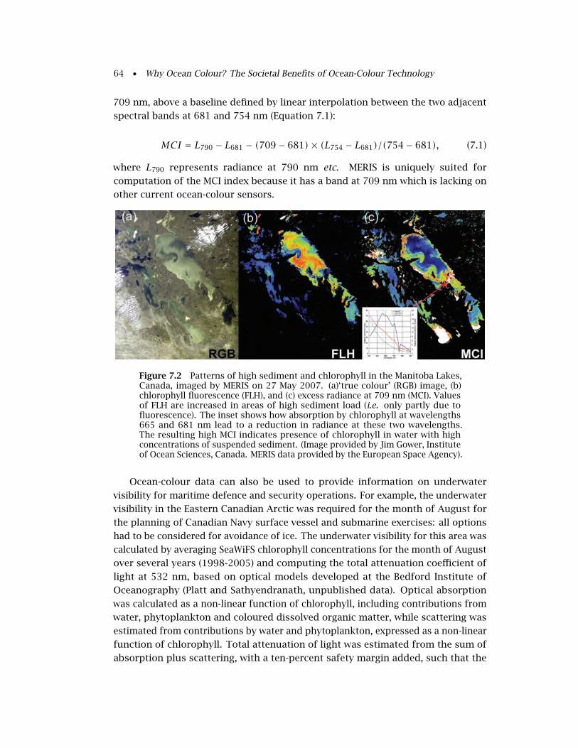
64 • Why Ocean Colour? The Societal Benefits of Ocean-Colour Technology
709 nm, above a baseline defined by linear interpolation between the two adjacent
spectral bands at 681 and 754 nm (Equation 7.1):
MCI = L790 − L681 − (709− 681)× (L754 − L681)/(754− 681), (7.1)
where L790 represents radiance at 790 nm etc. MERIS is uniquely suited for
computation of the MCI index because it has a band at 709 nm which is lacking on
other current ocean-colour sensors.
Figure 7.2 Patterns of high sediment and chlorophyll in the Manitoba Lakes,Canada, imaged by MERIS on 27 May 2007. (a)‘true colour’ (RGB) image, (b)chlorophyll fluorescence (FLH), and (c) excess radiance at 709 nm (MCI). Valuesof FLH are increased in areas of high sediment load (i.e. only partly due tofluorescence). The inset shows how absorption by chlorophyll at wavelengths665 and 681 nm lead to a reduction in radiance at these two wavelengths.The resulting high MCI indicates presence of chlorophyll in water with highconcentrations of suspended sediment. (Image provided by Jim Gower, Instituteof Ocean Sciences, Canada. MERIS data provided by the European Space Agency).
Ocean-colour data can also be used to provide information on underwater
visibility for maritime defence and security operations. For example, the underwater
visibility in the Eastern Canadian Arctic was required for the month of August for
the planning of Canadian Navy surface vessel and submarine exercises: all options
had to be considered for avoidance of ice. The underwater visibility for this area was
calculated by averaging SeaWiFS chlorophyll concentrations for the month of August
over several years (1998-2005) and computing the total attenuation coefficient of
light at 532 nm, based on optical models developed at the Bedford Institute of
Oceanography (Platt and Sathyendranath, unpublished data). Optical absorption
was calculated as a non-linear function of chlorophyll, including contributions from
water, phytoplankton and coloured dissolved organic matter, while scattering was
estimated from contributions by water and phytoplankton, expressed as a non-linear
function of chlorophyll. Total attenuation of light was estimated from the sum of
absorption plus scattering, with a ten-percent safety margin added, such that the

Ocean-Colour Radiometry and Water Quality • 65
estimates of visibility were conservative by the same amount. Horizontal visibility
is generally taken to be a linear multiple of the reciprocal of total attenuation. The
multiplication factor given in the literature is somewhat variable, around 4.8, but a
more conservative figure of 4.0 was used in this study. In the map produced (Fig.
7.3), there are striking variations in horizontal visibility, in particular an abrupt
reduction in visibility at the mouth of the Hudson Strait (south of Baffin Island). On
a Canadian Navy submarine voyage to the area, this figure provided an indication of
turbidity/visibility, and the ranges were found to be remarkably accurate.
Figure 7.3 Estimated underwater visibility (m) in the Eastern Canadian Arcticfor the month of August, based on SeaWiFS climatological records (Platt andSathyendranath, unpublished data).
7.3 Coastal Eutrophication
The process of eutrophication is the ecosystem’s response to an excess of nutrients
commonly issued from human activities through river runoff, direct inputs from
urban and industrial waste treatment, and atmospheric pollution. According to
Andersen et al. (2006), eutrophication is defined as ‘the enrichment of water by
nutrients, especially nitrogen and/or phosphorus and organic matter, causing an
increased growth of algae and higher forms of plant life to produce an unacceptable
deviation in structure, function and stability of organisms present in the water, and
to the quality of water concerned, compared to reference conditions’. The increase

66 • Why Ocean Colour? The Societal Benefits of Ocean-Colour Technology
in nutrients results in an escalation in photosynthesis and production of organic
carbon, which in turn can reduce the water transparency and oxygen availability at
depth, causing irreversible loss of habitats and mortality.
Nutrient pollution is one of the most severe and widespread environmental
threats to enclosed and semi-enclosed seas, estuaries and bays. For example, the
Black Sea ecosystem has been severely damaged by eutrophication over the past 30
to 40 years, with massive loads of anthropogenic nutrients entering the sea from the
major river systems, especially the Danube. Subsequent phytoplankton growth and
changes in the water transparency over the entire basin have negatively impacted
the rest of the ecosystem, with a loss of biodiversity due to oxygen depletion at
depth. This process is reflected in the optical signature of the Black Sea. Figure 7.4
shows the contrasting features of the Black Sea when compared with the rest of the
Mediterranean basin.
Figure 7.4 True-colour image captured by SeaWiFS on 14 June 2000, showinglarge amounts of reflecting material (phytoplankton biomass) in the Black Sea,contrasting with the clearer eastern Mediterranean waters (Credit: Ocean BiologyProcessing Group, NASA/GSFC and GeoEye).
7.3.1 Eutrophication Index in the Mediterranean Sea
Although Mediterranean waters are classified as oligotrophic, several alarming cases
of eutrophication have been recorded in coastal regions and enclosed bays, such
as in the Northern Adriatic Sea where the United Nations Environment Programme
established an ‘Eutrophication Monitoring Strategy’ in its Mediterranean Action Plan
(UNEP, 2003). This strategy proposed that each Mediterranean country establish a
monitoring program to sample a minimal set of parameters (Table 7.2). The plan

Ocean-Colour Radiometry and Water Quality • 67
mentions explicitly the use of optical remote sensing as a complementary technique
to support the measurements of some of these parameters including chlorophyll,
suspended material distributions, and turbidity. In addition, it is recommended
that remotely-sensed data be incorporated with in situ observations to provide
eutrophication-indicator maps on a routine basis.
The set of parameters highlighted in Table 7.2 in bold are used to calculate a
trophic index (TRIX) as defined by Vollenweider et al. (1998) and Giovanardi and
Vollenweider (2004), on the basis of 10 years of data collected along the northwestern
Adriatic coast. The trophic index combines factors that describe phytoplankton
biomass and nutrient availability as follows:
TRIX = [log10(Chl.dO.DIN.TP)− (k)]/m, (7.2)
where Chl is the chlorophyll-a concentration (i.e. phytoplankton biomass) in µg l−1,
dO is oxygen, as absolute % deviation from saturation,DIN is the sum of all dissolved
inorganic nitrogen compounds in µg l−1, TP is total phosphorus in µg l−1, and the
coefficients k and m are scale coefficients of the trophic index based on the upper
and lower limits of the parameters. Since 1999, TRIX has been incorporated into the
Italian water legislation (Casazza et al., 2003) with values distributed in 4 classes,
ranging from ‘high’ environmental state (TRIX values from 2 to 4), i.e., good water
transparency, well distributed dissolved oxygen in the entire water column, to ‘poor’
environmental state (TRIX values from 6 to 8), i.e., highly turbid waters, persistence
of hypoxic/anoxic bottom layers. The Mediterranean Action Plan proposes to extend
the use of TRIX in all Mediterranean coastal waters (UNEP, 2003).
Table 7.2 Mandatory parameters to be monitored by each country following the guidelinesof the UNEP/MED POL monitoring strategy for assessing Mediterranean eutrophication(adapted from UNEP, 2003). Parameters highlighted in bold (right hand column) are used tocalculate a trophic index (TRIX, see text).
Temperature (°C) Dissolved Oxygen (mg l−1)
pH Chlorophyll a (µg l−1)
Transparency /Secchi depth (m) Nitrate (NO3-N, µg l−1)
Salinity (psu) Ammonium (NH4-N, µg l−1)
Total Nitrogen (N, mol l−1) Nitrite (NO2-N, µg l−1)
Silicate (SiO2, mmol l−1) Total phosphorus (P, µg l−1)
Phytoplankton (number and species composition) Orthophosphate (P-PO4, µg l−1)
Optical remote sensing can contribute to the calculation of TRIX by providing
chlorophyll values at a suitable frequency with respect to coastal and lake dynamics.
However, as an index of primary productivity, the calculation of TRIX requires the
knowledge of parameters not accessible from remote sensing. A regional application
of TRIX based on remote sensing would require the area to be partitioned into
dynamic ecological provinces, within which field-derived quantities can reasonably
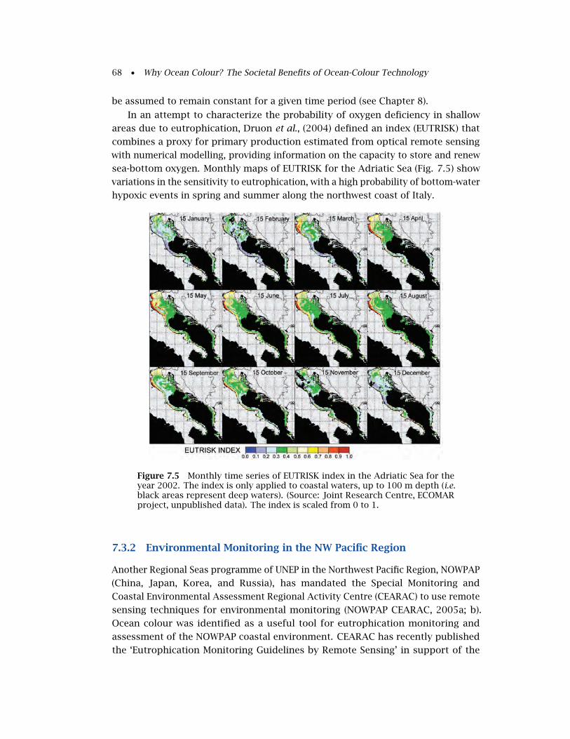
68 • Why Ocean Colour? The Societal Benefits of Ocean-Colour Technology
be assumed to remain constant for a given time period (see Chapter 8).
In an attempt to characterize the probability of oxygen deficiency in shallow
areas due to eutrophication, Druon et al., (2004) defined an index (EUTRISK) that
combines a proxy for primary production estimated from optical remote sensing
with numerical modelling, providing information on the capacity to store and renew
sea-bottom oxygen. Monthly maps of EUTRISK for the Adriatic Sea (Fig. 7.5) show
variations in the sensitivity to eutrophication, with a high probability of bottom-water
hypoxic events in spring and summer along the northwest coast of Italy.
Figure 7.5 Monthly time series of EUTRISK index in the Adriatic Sea for theyear 2002. The index is only applied to coastal waters, up to 100 m depth (i.e.black areas represent deep waters). (Source: Joint Research Centre, ECOMARproject, unpublished data). The index is scaled from 0 to 1.
7.3.2 Environmental Monitoring in the NW Pacific Region
Another Regional Seas programme of UNEP in the Northwest Pacific Region, NOWPAP
(China, Japan, Korea, and Russia), has mandated the Special Monitoring and
Coastal Environmental Assessment Regional Activity Centre (CEARAC) to use remote
sensing techniques for environmental monitoring (NOWPAP CEARAC, 2005a; b).
Ocean colour was identified as a useful tool for eutrophication monitoring and
assessment of the NOWPAP coastal environment. CEARAC has recently published
the ‘Eutrophication Monitoring Guidelines by Remote Sensing’ in support of the

Ocean-Colour Radiometry and Water Quality • 69
implementation of an integrated marine environmental monitoring program in
the region (NOWPAP CEARAC, 2007). It was also recommended that ocean-colour
remote sensing techniques be used for case studies on harmful algal blooms
as well as assessment of the eutrophication status in this region from 2008.
Several web portal sites have been created at CEARAC showing the use of satellite
remote sensing (http://www.cearac-project.org/wg4/portalsite/), oil spill monitoring
(http://cearac.poi.dvo.ru/en/main/about/) and Marine Environmental Protection of
the Northwest Pacific Region (http://www.nowpap3.go.jp/jsw/eng/).
7.4 Suspended Matter in the Coastal Zones
Plumes of turbid water are quite a frequent phenomenon in coastal waters, in
particular in shallow soft bottom seas and in the mouth of rivers and estuaries (Fig.
7.6, see also Figs. 2.4 and 9.5). Turbidity is caused by a variety of particles in the
Figure 7.6 Envisat MERIS satellite image showing plumes of turbid wateremanating from the mouth of the Yangtze River, China, on 15 March, 2008(Credit: European Space Agency).
water, some of mineral origin, such as clay particles, and others of organic origin.
Collectively, these particles are referred to as Suspended Particulate Matter (SPM) or
Total Suspended Matter (TSM). The mineral portion primarily originates from the
fine fraction of sediments, which are transported by rivers into the sea or, in shallow
water, re-suspended from the sea floor by waves or tidal currents. SPM represents an
extremely large amount of material, which is transported over long distances within
70 • Why Ocean Colour? The Societal Benefits of Ocean-Colour Technology
the coastal sea. Other sources of the inorganic fraction include dust from deserts or
volcanoes, and fragmented skeletons of organisms such as coccolithophores, diatom
shells etc.
The organic portion of suspended material, i.e. the detritus, is composed of
decaying fragments of organisms or fecal material. The different particles can
form complex flakes of an undefined structure, which act as a substrate for many
microorganisms that colonize the surface and holes in the flakes, and live by
decomposing and mineralizing the organic material. Due to the high organic content
(including the attached microbes), detritus is an important food source for many
benthic organisms. Furthermore, the complex large surface area of the flakes
absorbs a number of different organic and inorganic trace substances, which are also
transported with the suspended material. Finally, SPM absorbs and backscatters light
and thus reduces the available solar radiance for photosynthesis by phytoplankton,
benthic algae and seagrass.
Due to its diverse role, the formation and transformation, distribution and
transport of SPM in the sea is of wide interest in various fields of marine science
including marine biology and geochemistry, but also for monitoring the water
quality, studying coastal erosion and the underwater light field and visibility. Due
to the complex nature of SPM, transport and distribution cannot be observed in a
representative way by ship cruises, nor can it simply be modelled as in the case of a
conservative tracer like salinity. Only observations using aerial surveys and satellite
data enable us to reveal the extremely complex distribution patterns and temporal
variability. Thus, observations with a high spatial and temporal resolution are needed
to map the distribution and analyze the transport mechanism. On the other hand,
satellite observations are limited by clouds and show only the distribution of the
upper few metres. To provide a complete view, as well as time series with a high
temporal frequency, it is necessary to combine observations and simulations using
data assimilation techniques.
ESA’s MERIS sensor provides the potential to map SPM distributions in coastal
zones due to its relatively high spatial resolution (300 nm) and 15 spectral bands in
the visible and NIR spectral range. NASA’s MODIS sensor provides more frequent
coverage at a slightly higher spatial resolution (250 m), but has only one 250 m
waveband centred in the visible, while SeaWiFS and AVHRR are also useful for
mapping SPM distribution. The SPM component can be separated from the absorption
by phytoplankton and dissolved organic matter using an artificial neural network
which is currently used in the MERIS ground processor as the standard algorithm
to determine SPM concentrations from the bi-directional water-leaving radiance
reflectance (Fig. 7.7). These data have been used for assimilation into a SPM transport
model for the North Sea.
The algorithm to determine SPM and other components from MERIS water-leaving
radiance reflectance is based on an artificial neural network (NN) (Doerffer and
Schiller, 2007). This NN in turn is trained with a large data set of simulated bi-

Ocean-Colour Radiometry and Water Quality • 71
Figure 7.7 (a) Total suspended matter (TSM) derived from a MERIS scene overthe North Sea on 27 March 2007, using the Case-2 R-BEAM processor, and(b) corresponding signal depth, z90max . (Credit: Image provided by RolandDoerffer (GKSS, Germany), MERIS data provided by the European Space Agency).
directional radiance reflectances using Hydrolight (Mobley, 1994) as the radiance
transport model. The underlying bio-optical model in turn is based on absorption and
scattering measurements of a variety of coastal waters with concentrations of SPM
up to 50 mg l−1. Output of the NN are the three optical components (1) absorption
coefficient of phytoplankton pigment, (2) absorption coefficient of dissolved organic
matter (yellow substance plus detritus) and (3) scattering by all particulate matter
(as defined by the pore size of the filter of ca. 0.2 - 0.45 µm). These coefficients
are then used to compute the concentrations of chlorophyll and suspended matter
using empirical relationships.
Another variable necessary to assimilate MERIS data into the model is the
computation of the penetration depth. For this purpose, the maximum signal depth
was computed using the optical properties of the three components. It is defined
as the water depth of the surface water layer from which 90% of the water-leaving
radiance originates, and is determined for each pixel from the three MERIS bands
with the lowest downwelling irradiance attenuation coefficients. This depth was
used to compare the concentrations from MERIS and the SPM transport model.
The SPM transport model is a hydrodynamical model. It includes tidal
currents, waves and bioturbation as the most important processes, which determine
sedimentation, re-suspension, transport and distribution in the coastal sea. A map of
sediment distribution in the North Sea forms the basis for computing re-suspension.
Important parameters such as the erosion depth and the vertical exchange coefficients
were adjusted at the beginning of the development using satellite data of SPM from
MOS (Modular Optical Spectrometer). The SPM model calculates distributions of
three SPM fractions with different settling velocities in the water column and the

72 • Why Ocean Colour? The Societal Benefits of Ocean-Colour Technology
Figure 7.8 An example of data assimilation using the optimum interpolationmethod: a) surface concentration as calculated with the SPM transport model; b)surface sediment concentration derived from MERIS on 22 March 2003; c) modelresult after assimilating the MERIS data and d) difference between model resultsbefore and after data assimilation. (Credit: Image provided by Gerhard Gayerand Mikhail Dobrynin (GKSS, Germany), MERIS data provided by the EuropeanSpace Agency).
corresponding fine sediment fractions in the first 20 cm from the bottom.
The results were compared to MERIS satellite data and to in-situ measurements,
and a quality control system for the satellite data was developed. Next, the satellite
data were assimilated into the model using a sequential optimum interpolation
scheme (Fig. 7.8). The results show a significant improvement with assimilation. In
particular, an overestimation of SPM is avoided (Fig. 7.9). However, further work is
required to improve the assimilation procedure. From the point of view of satellite
data providers, it is necessary to supply uncertainty estimates on a pixel-by-pixel
basis. From the modeller’s perspective, the weighting of satellite data with respect
to these uncertainties, and in particular to the areas which are masked by clouds,
have to be optimized.
7.5 Concluding Remarks
In spite of the unresolved problems surrounding the quantitative interpretation of
water colour in complex turbid water environments, optical remote sensing remains
a unique and useful tool to assess water quality at synoptic scales. Its applications

Ocean-Colour Radiometry and Water Quality • 73
Figure 7.9 Seasonal mean TSM surface concentrations (g m−3) calculated bythe model with assimilation of satellite data for (a) the calm summer period,15 April - 15 October, and (b) the winter period with more storms, 15 October- 15 April. The same calculation without data assimilation is shown in (c) forsummer and in (d) for winter conditions. (Image provided by Gerhard Gayerand Mikhail Dobrynin (GKSS, Germany), MERIS data provided by the EuropeanSpace Agency).
in operational management of aquatic environments are growing and capturing the
interest of more end-users in different sectors. In parallel, the scientific and technical
communities continue to search for better bio-optical models in optically-complex
waters. Recent development of hyperspectral sensors (Bukata and Helbig, 2004;
Dickey 2004) which provide coverage over the full spectrum of visible wavelengths,
offer new opportunities to discriminate optical boundaries, and hence, to classify
turbid waters and quantify individual components such as phytoplankton species
and chemical compounds.

74 • Why Ocean Colour? The Societal Benefits of Ocean-Colour Technology

Chapter 8
A Window on the State of the Marine Ecosystem
Trevor Platt and Shubha Sathyendranath
8.1 Ecological Indicators
There is a developing global consensus that management of the oceans should be
ecosystem based, and that the integrity of the ecosystem should not be compromised
(Garcia and Cochrane, 2005). A requirement has therefore developed for ecological
indicators that quantify the elusive ecosystem properties of health, vigour and
resilience. Indicators provide objective metrics of ecosystem properties that can be
applied serially and operationally to detect changes that may occur in response to
environmental perturbation.
A variety of ecosystem indicators have been proposed (reviewed by Rice, 2003;
Platt and Sathyendrenath, 2008). These range from theoretically-simple indicator
species, which, like the canary in a coal mine, convey information on the entire
ecosystem, to quantitative attributes of the ecosystem revealed by ecosystem models.
An ideal ecosystem indicator is objective, quantifiable in standard units, and has
a non-contentious meaning. It should be available at high spatial and temporal
resolution, in a cost-effective manner, to permit the construction of time series
such that ecosystem change can be detected in a timely manner. Remotely-sensed,
ocean-colour radiance data meet these stringent conditions. The retrieved variable,
phytoplankton biomass, is an important property of the ocean ecosystem, broadly
understood and expressible in standard units. Resolution in space and repeat
frequency of sampling are beyond reproach.
Several metrics developed from serial ocean-colour data may prove to be useful
indicators of the state of the ocean ecosystem (Table 8.1). Of course, it is not
expected that ocean colour could provide indicators on all properties relevant
to ecosystem-based management, but certainly it will provide, in an extremely
cost-effective manner, objective indices of the near-real-time condition of the
pelagic system. For example, autotrophic biomass and primary production, both of
which can be estimated from ocean-colour data, are important pelagic ecosystem
properties. The high frequency repeat sampling of ocean-colour data provides
sufficient data to describe seasonal dynamics and make interannual comparisons
75

76 • Why Ocean Colour? The Societal Benefits of Ocean-Colour Technology
(Yamada and Ishizaka, 2006; Wu et al., 2008a). The AVHRR series of SST is a source
of complementary data about the physical environment, on the same scales of time
and space.
Table 8.1 Ecological indicators of the pelagic ocean that can be derived from ocean-colourradiometry (Platt and Sathyendranath, 2008).
Indicator Label Dimensions
Initiation of spring bloom bi [T]
Amplitude of spring bloom ba [ML−3]
Timing of spring maximum bt [T]
Duration of spring bloom bd [T]
Total production in spring bloom bp [ML−2]
Annual phytoplankton production PY [ML−2]
Generalised phytoplankton loss rate L [ML−3T−1]
Integrated phytoplankton loss LT [ML−3]
Annual-scale f -ratio f Dimensionless
Spatial variance in biomass field σ 2B [M2L−6]
Spatial variance in production field σ 2P [M2L−4]
Phytoplankton functional types NA NA
Delineation of biogeochemical provinces NA NA
Phytoplankton size structure s Dimensionless
Ocean colour radiance data streams provide a rich resource for construction of
time series, where serial images can be arranged to display the seasonal evolution of
the chlorophyll fields, and the variations between years in these seasonal cycles (Platt
and Sathyendrenath, 1988). The significance of these time series is that they offer
a way to quantify the response of the ocean ecosystem to perturbation, natural or
anthropogenic. They provide a rapid and cost-effective way to detect change in the
magnitude and spatial distribution of a major ecosystem property, the autotrophic
biomass.
8.1.1 Indicators Describing the Spring Bloom
In temperate latitudes, the spring phytoplankton bloom is the dominant component
of the seasonal cycle. At each and every pixel in the region of interest, the spring
bloom can be characterized with respect to amplitude (ba), using the chlorophyll time
series (Fig. 8.1, Table 8.1). Using satellite ocean-colour data we can also establish
objectively, using threshold criteria, the time of the spring bloom initiation (bi),the time of the maximum (bt) and also the duration of the bloom (bd). Because
these indices (bi, bt and bd) depend only on timing and not on absolute magnitudes
(provided the threshold criteria are relative rather than absolute), they are not
compromised by any problems arising from merging of different data streams. Using
the time series, we can examine how these properties vary between years.

A Window on the State of the Marine Ecosystem • 77
Figure 8.1 Objective characterization of the properties of a spring phyto-plankton bloom at a given pixel from time series of chlorophyll concentration.Defining characteristics are amplitude, initiation, timing of maximum andduration (from Platt and Sathyendranath, 2008).
The spring bloom is the most important event in the seasonal cycle of the
ecosystem over much of the ocean. The reproduction of many organisms is timed
to coincide with this event and fluctuations between years in its timing may have
profound consequences for components of the ecosystem other than phytoplankton.
For example, the Cushing-Hjort hypothesis, also known as the match-mismatch
hypothesis, relates timing of blooms with timing of spawning and larval mortality
of organisms higher in the food chain than phytoplankton. This hypothesis is very
difficult to address using only ships as oceanographic platforms. However, it has
proved to be more tractable using ocean-colour radiometry (Platt et al., 2003). Thus,
when we attempt to account for fluctuations in the abundance of marine species of
commercial interest, we now have the possibility to consider the potential effect of
changes in the ecosystem itself as a contributing factor.
8.1.2 Indicators Describing Phytoplankton Production
Ocean-colour data can be used to estimate phytoplankton production, also called
primary production (Platt and Sathyendranath 1988; 1993; 1999) from which time
series can be developed. An operational procedure is also available (Platt et al.,
2008). The primary production time series can also be used to describe the timing
of the spring bloom. As a rate measurement, primary production can be integrated
through time to estimate either the total production in the spring bloom (bp) or total
annual production (PY ). These estimates of production are key measurements of
ecosystem capacity. For example, the spring bloom production is a lower bound on
the annual new production, where new production is that production supported by
nitrogen supplied from outside the surface layer. Theoretically, the new production
represents the nitrogen equivalent that can be removed from the pelagic zone in one
year without impacting the overall productivity of the system. Further, the spring
bloom production, as a minimal estimate of new production, can be used to calculate
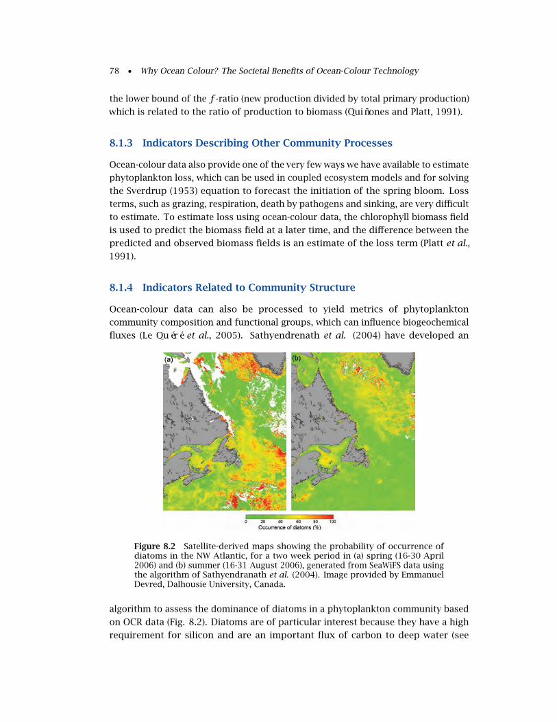
78 • Why Ocean Colour? The Societal Benefits of Ocean-Colour Technology
the lower bound of the f -ratio (new production divided by total primary production)
which is related to the ratio of production to biomass (Quiñones and Platt, 1991).
8.1.3 Indicators Describing Other Community Processes
Ocean-colour data also provide one of the very few ways we have available to estimate
phytoplankton loss, which can be used in coupled ecosystem models and for solving
the Sverdrup (1953) equation to forecast the initiation of the spring bloom. Loss
terms, such as grazing, respiration, death by pathogens and sinking, are very difficult
to estimate. To estimate loss using ocean-colour data, the chlorophyll biomass field
is used to predict the biomass field at a later time, and the difference between the
predicted and observed biomass fields is an estimate of the loss term (Platt et al.,
1991).
8.1.4 Indicators Related to Community Structure
Ocean-colour data can also be processed to yield metrics of phytoplankton
community composition and functional groups, which can influence biogeochemical
fluxes (Le Quéré et al., 2005). Sathyendrenath et al. (2004) have developed an
Figure 8.2 Satellite-derived maps showing the probability of occurrence ofdiatoms in the NW Atlantic, for a two week period in (a) spring (16-30 April2006) and (b) summer (16-31 August 2006), generated from SeaWiFS data usingthe algorithm of Sathyendranath et al. (2004). Image provided by EmmanuelDevred, Dalhousie University, Canada.
algorithm to assess the dominance of diatoms in a phytoplankton community based
on OCR data (Fig. 8.2). Diatoms are of particular interest because they have a high
requirement for silicon and are an important flux of carbon to deep water (see

A Window on the State of the Marine Ecosystem • 79
Figure 8.3 Left: Patterns of floating Sargassum in the Gulf Stream, imagedby MERIS (300 m resolution) on 22 October 2007 as MCI. Right: TOA radiancespectra for the Sargassum region indicated by arrow (red line), and for nearbyclear water (green line). The difference (blue line, values on right axis) showsthe ‘red edge’ characteristic of land vegetation, with a shift in wavelength thatresults in a high value of MCI (after Gower and King, 2008. Image data providedby the European Space Agency).
Chapter 5). Alvain et al. (2005) have also developed a procedure to index functional
groups, estimates of which can be used in the most recent ocean carbon cycle models.
Given that it carries information on trophic status or chlorophyll biomass, ocean
colour may also be indicative of the size structure of the phytoplankton community
(Chisholm, 1992; Bouman et al., 2005; Platt et al., 2005), the more eutrophic water
being dominated by larger phytoplankton than oligotrophic waters. Further, the
absorption spectrum derived from ocean-colour data can also contain information
on size structure (IOCCG, 2006). For example, Devred et al. (2006) used a two-
component model in a variety of oceanic regimes, to estimate the proportion of
picoplankton and nanoplankton (see also ‘algal effective diameter’, Fig. 9.8).
In another study, Gower and King (2008) made use of the MERIS Maximum
Chlorophyll Index (MCI) to map of the distribution and movement of the floating
seaweed, Sargassum, in the Gulf of Mexico and western Atlantic (Fig. 8.3, see also
Chapter 7). Their data indicated strong growth early in the year in the Gulf of Mexico,
with Sargassum moving out into the Atlantic each year in July and August.
8.1.5 Indicators Related to Variance in Chlorophyll Fields
There is a growing belief among those that study the population dynamics of fish,
that only a small proportion of individuals contribute to recruitment of the next
cohort (Berkeley et al., 2004), with successful spawners being those that spawn
in the time and place with the most favourable conditions for larval survival and
growth. Berkeley et al. (2004) argue that networks of marine protected areas that
protect a broad age structure and a broad range of habitats are necessary to conserve

80 • Why Ocean Colour? The Societal Benefits of Ocean-Colour Technology
marine populations. The location of these protected areas could be informed by the
chlorophyll time series and the indices derived from these time series. Spatial and
temporal variance in the chlorophyll time-series could inform the choice of marine
protected areas. For example, we might want to protect areas where phytoplankton
biomass or production is relatively high.
8.2 Spatial Structure of the Ocean Ecosystem at Large ScaleBiogeographical Provinces
Many of the important applications of ocean colour deal with problems that are
global in scope. An example is the role of the ocean in the planetary carbon cycle and
its significance for climate change. Although the issues are global-scale in character,
from an ecological point of view we cannot treat the ocean as being everywhere the
same. We can perceive the ocean ecosystem as a suite of contiguous subsystems
within each of which the internal interactions dominate over the interactions between
subsystems. Thus, the central ocean gyres are different, ecologically, from upwelling
regimes, and we expect that the ecophysiological rates in the two environments will
be different. We call the regions, so defined, biogeochemical provinces (Platt and
Sathyendrenath, 1988). In making global assessments of ecosystem performance,
we may therefore adopt an approach in which the contributions of each province
would be calculated separately and the results aggregated to the global scale.
Figure 8.4 Biogeochemical provinces in the ocean, adapted from Longhurst (2006).
To implement this approach, we need first a scheme for partitioning the ocean
into a suite of biogeochemical provinces. An example is that produced by Longhurst
(2006). Here, the assumption is that phytoplankton ecology is under the control of
physical forcing and the partition is made according to the large-scale patterns in the
forcing that is relevant to the phytoplankton. The resultant partitioning yields some

A Window on the State of the Marine Ecosystem • 81
sixty provinces at the global scale (Fig. 8.4). In his original publication, conceived
with imagery from CZCS, the boundaries between these provinces were rectilinear
and schematic in character. It was understood that the boundaries would shift
with seasonal progression and between years, in other words that the boundaries
would be dynamic. If we want to delineate the boundaries at any particular moment,
Figure 8.5 Biogeochemical provinces of the Northwest Atlantic Ocean forthe year 2006, determined objectively using OCR data. (Image provided byEmmanuel Devred, Dalhousie University, Canada).
remotely-sensed data on ocean colour provide the most useful resource, given that
they afford a global-scale view of the pelagic ocean (Platt and Sathyendrenath, 1999;
Platt et al., 2005; Devred et al., 2007). In the first instance, OCR is the key by which
we can translate the diagrammatic scheme of Longhurst into a less-rigid scheme
that reflects the reality of the day (Fig. 8.5). Further, serial study of ocean-colour
imagery allows us to see the shifts in the province boundaries between seasons (Fig.
8.6) and between years.
A partition of the ocean constructed in this way has many applications in
oceanography and biogeochemistry. It provides an oceanographic context for
understanding particular findings. It gives a framework for implementation of
algorithms that proceed by weighted integration over diverse spatial blocs. It allows
the rich data set acquired by remote sensing to complement the sparse data acquired
using ships. Further, it also provides the ideal template for the placement of marine
protected areas, which as Berkeley et al. (2004) argue, may be most beneficial if
placed in different habitats within biogeographical and oceanographic regions.
The development of these methods has been stimulated strongly by the
availability of ocean-colour data, and their implementation would be very difficult, if
not impossible, without access to ocean-colour data. The first partitioning scheme
by Longhurst was inspired by the synoptic chlorophyll fields derived from CZCS,

82 • Why Ocean Colour? The Societal Benefits of Ocean-Colour Technology
Figure 8.6 Dynamic borders of biogeochemical provinces in the NW Atlanticin June and October over 3 years (2002-2004). Colour scheme is the same as forFig. 8.5 (Image provided by Emmanuel Devred, Dalhousie University, Canada).
and its refinement to incorporate short-time variability is achievable only through
currently-flying sensors. To this extent, the disaggregation of the ocean into a suite
of biogeochemical provinces as an aid to research and understanding can be seen as
a major contribution of the ocean-colour initiatives undertaken some thirty years
ago.
8.3 Conclusions
Even with only two remotely-sensed variables (chlorophyll and temperature), a rich
set of ecological indicators can be derived (Table 8.1). Access to ancillary in situ data
improves the interpretation of ocean-colour time series. Although one of the defining
advantages of the use of ocean colour in the development of ecosystem indicators is
the potential to provide indicators on an operational basis, further research holds
promise of improved understanding of the ecosystem and indicators of health,
integrity and resilience. With an emphasis on quality control, remotely-sensed data
can be useful for construction of time series. Time series provide cost-effective basis
for development of ecological indicators, averaged at appropriate time and space
scales. The 10-year series of SeaWiFS has already yielded some interesting results,
and we should strive to maintain continuity of a reliable ocean-colour data stream.

Chapter 9
Hazards: Natural and Man-Made
Heidi Dierssen, James Acker, Stewart Bernard and Grant Pitcher
Ocean basins, regional seas, and coastal margins are subject to a variety of hazards
that can occur suddenly, periodically, or slowly resulting from changes to climate
and the environment. Broadly defined by the United States Department of Defense,
a hazard is "Any real or potential condition that can cause injury, illness, or death to
humans; damage to or loss of a system, equipment or property; or damage to the
environment". Episodic hazards can restructure the coastal zone, greatly impacting
marine and estuarine ecosystems as well as residential communities residing along
the coasts. Over one-third of the total human population, nearly 2.4 billion people,
lives within 100 km of an oceanic coast, a fact emphasized by the devastating tsunami
in the Indian Ocean in 2004. Hazardous events, such as hurricanes and tsunamis,
often originate in areas distant from where they eventually have the most significant
impact, and occur on space and time scales that can only be resolved from satellite
imagery. While some hazards are considered ‘natural’ in origin (e.g., earthquakes,
storms), anthropogenic changes to the environment have increasingly contributed
to the frequency, magnitude, and duration of many hazards confronting humans
and the environment.
The human population is growing; more people are living closer to the
ocean and the human footprint on the oceans, particularly the coastal zone, is
markedly increasing. In order to better evaluate relationships between natural and
anthropogenic hazards, the following sections categorize hazards based on their
relative time scales. Hazards can be broadly divided into two categories: acute
versus chronic (Table 9.1). Some examples of acute hazards include tropical storms,
flooding and river runoff, earthquakes leading to tsunamis, spills of toxic or noxious
substances, harmful or toxic organisms, and icebergs. Long-term or chronic hazards
facing marine ecosystems include increasing sea surface temperature, acidification
(lower pH), increased sea level, changing water properties e.g. due to influx of glacial
melt-water, and increased eutrophication due to nutrient fertilization in the coastal
zone. Chronic changes to the ocean environment provide new conditions to which
marine organisms must acclimate for survival, and new habitats for water-borne
pathogens to be spread. Chronic hazards also have the potential to contribute to
acute hazards. For example, increased sea surface temperatures can increase the
83

84 • Why Ocean Colour? The Societal Benefits of Ocean-Colour Technology
frequency and intensity of tropical storms (Emanuel, 2005; Webster et al., 2005).
Table 9.1 presents a list of some known hazards that confront the world’s oceans
and the resulting impacts on the oceanic ecosystems, both to physical characteristics
and the ecosystems.
Table 9.1 Selected hazards impacting the ocean.
Hazard Impact
Acute Hazard
Tropical storm Sediment plumes, beach erosion, loss of benthic habitats, resuspension oftoxins, increased pathogens
Tsunami Sediment plumes, beach erosion, loss of benthic habitats, resuspension oftoxins, increased pathogens
Chemical spill Toxic plumes, mortality of plankton/nekton
Flooding/riverrunoff
Sediment plumes, anoxia, hypoxia, harmful algal blooms, increased toxinsand pathogens
Iceberg Navigation problems, altered sea ice patterns and associated food webs
Chronic Hazard
Chronic sea surfacewarming
Altered thermohaline circulation, coral bleaching, delay or prevention ofsea ice formation, seasonal timing altered, increased tropical storms withassociated impacts, altered food web, increased pathogens
Increasing acidity Prevention of calcification (corals, pteropods, etc.), altered food web
Rising sea level Coastline changes, altered benthic habitats
Glacial melt-water Stabilized water column, prevention of deep-water formation/circulation,decreased light penetration, increased productivity, altered food web
Nutrient fertilization Harmful algal blooms, anoxia, hypoxia, loss of benthic habitats, alteredfood web
The following sections present the potential uses of ocean-colour radiometry
for detecting episodic hazards and the impacts of both acute and chronic hazards
on marine ecosystems. Impacts on the terrestrial environment and human life and
property are not directly discussed here, but the oceans are the largest publicly-
shared domain and consequences on marine ecosystems affect all spheres of life.
9.1 Monitoring Hazards with Ocean-Colour Radiometry
Ocean-colour sensors are not specifically designed to make the very detailed
observations required for high temporal tracking of episodic events and high spatial
resolution to resolve fine-scale features. Many acute hazards, however, can be
observed using the current suite of ocean-colour satellites. Polar orbiting ocean-

Hazards: Natural and Man-Made • 85
colour sensors have repeat global coverage every 2-3 days at the equator, with
daily coverage at higher latitudes. In the mid-latitudes, hurricanes can be tracked
nearly daily via the SeaWiFS, MODIS and MERIS sensors (Fig. 9.1). These true colour
images can be derived at 250 m resolution, a finer resolution than available from
geostationary platforms like the current weather satellites (e.g., GOES). Such high
resolution imagery can resolve the track and spatial extent of intense storms with
greater accuracy and aid in development of better predictive storm models.
Figure 9.1 Hurricane Ivan over the Gulf Coast of the U.S, captured by SeaWiFSon 15 September 2004. Ivan attained Category 5 strength with winds reaching270 km h−1. (Credit: Ocean Biology Processing Group, NASA/GSFC and GeoEye).
Earthquakes that occur along the ocean bottom can displace the seafloor several
metres and result in large oceanic waves called ‘tsunamis.’ Tsunamis can move at
roughly 640 km hr−1 across the seafloor. The waves slow down when they reach
shallow water near land and the accompanying reduction in speed and wavelength
results in increased height and steepness as the wave’s energy is condensed in
a smaller water volume. As evident in the December 2004 tsunami that struck
southeast Asia, massive tsunami waves have been among the deadliest natural
disasters in modern history. Remotely-sensed imagery of tsunamis is more difficult
to obtain from traditional satellite platforms due to their rapid speed and fine spatial
scale. Moreover, nadir-viewing ocean-colour imagery does not necessarily detect
wave fields, unless they are associated with corresponding shifts in ocean colour.
However, multi-angle imagers, like the MISR (Multi-angle Imaging SpectroRadiometer)
instrument aboard the Terra satellite, have been used to detect roughness patterns
on the sea surface associated with large waves. The waves are made visible due to
the effects of changes in sea-surface slope on the reflected sun-glint pattern. For
example, imagery of wave patterns and wave-breaking associated with the devastating

86 • Why Ocean Colour? The Societal Benefits of Ocean-Colour Technology
December 2004 tsunami, were observed with MISR’s 46-degree forward pointing
camera, but were invisible to MISR’s nadir (vertical-viewing) imager (Fig. 9.2). MODIS-
Aqua data were used to assess the post-tsunami effects on chlorophyll and turbidity
in the area (Tan et al., 2007).
Figure 9.2 At approximately 05:15 UTC on 26 December, 2004, the Multi-angleImaging SpectroRadiometer (MISR) aboard the Terra satellite captured this imageof deep ocean tsunami waves about 30-40 km from Sri Lanka’s south-westerncoast. (Credit: NASA/GSFC/LaRC/JPL, MISR Team).
Episodic flooding of coastal regions due to intense storms or tsunamis can also
be observed with ocean-colour imagery. Land surfaces overlain by water have lower
spectral reflectance and the spectrum is generally limited to visible wavelengths;
separation of the land from water can thus be accomplished with relatively simple
techniques. To date, most of the remote sensing analyses of floods have primarily
been done with true or false colour images derived from the sensors aboard satellites
or portable airborne sensors, including airborne active lidars, and are verified with
time-series of images taken before and after a major flood event. Flood water can be
difficult to see in true colour satellite images, particularly when the water is muddy.
A combination of visible and infrared light can be used to make floodwaters more
obvious (see Fig. 9.3).
From the recent accomplishments in radiative transfer modelling in optically-
shallow water (as discussed further in the following sections on shallow water
bathymetry and benthic habitat characterization), potential exists for estimating the
water depth and water properties of flood regions using high resolution ocean-colour
imagery.
As snow accumulates on polar landmasses, it compacts and forms ice. As ice
builds up, it flows outward into floating shelves and is sloughed off or ‘calved’ from
the front of the glacier as an iceberg. Global warming has apparently increased the
rate of ice stream flow in Greenland (Zwally et al. 2002) and led to the disappearance
of Antarctic ice shelves. Icebergs can hinder navigation along shipping lanes and
significantly alter the water column properties. In addition, icebergs can disrupt
sea ice patterns, phytoplankton blooms and survival of higher trophic levels, such

Hazards: Natural and Man-Made • 87
Figure 9.3 These photos were captured by NASA’s MODIS-Terra sensor beforeand after the spring rains caused widespread flooding of the Mississippi Riverin March 2008. Water levels on the Mississippi River were still high on 7 April2008 (Credit: MODIS Rapid Response Team, NASA/ GSFC).
as pteropods (pelagic snails) and penguins (Arrigo et al., 2002; Seibel and Dierssen
2003). Ocean-colour imagery has been employed to identify and track the path of
icebergs. In March 2000, one of the largest icebergs ever recorded calved from the
eastern Ross Ice Shelf, Antarctica. In a few weeks the iceberg, named B-15, split into
several pieces, the largest of these being B-15A which has persisted in McMurdo
for several years (Fig. 9.4). Even this fragmented iceberg, approximately 160 km in
length and 200-270 m in thickness along its centerline, contained enough drinking
water to supply the world for several months. SeaWiFS imagery was also used to
assess the impact of icebergs on phytoplankton biomass (Schodlok et al., 2005).
Figure 9.4 True-colour image of the iceberg B-15A in McMurdo Sound,Antarctica, captured by NASA’s MODIS-Terra satellite on 13 December, 2004(Credit: Jeff Schmaltz, MODIS Land Rapid Response Team at NASA GSFC).

88 • Why Ocean Colour? The Societal Benefits of Ocean-Colour Technology
In addition, input of glacial melt-water into the coastal regions can change the
water clarity and enhance reflectance due to the addition of fine particles (i.e., ‘glacial
flour’), add potentially limiting nutrients like iron, enhance the stability of surface
waters, and impact sea ice cycles. The input of pulsed inputs of melt-water was
shown to increase productivity up to hundreds of kilometres offshore along the
Antarctic Peninsula (Dierssen et al., 2002).
Harmful impacts of phytoplankton blooms are often associated with the release
of biotoxins by certain species present in the algal assemblage. Marine biotoxins,
such as domoic acid, saxitoxins and okadaic acid are some of the most potent toxins
in the world and extremely dangerous. For some compounds, doses at the level of µg
kg−1 are more than sufficient to kill. Ocean colour cannot directly monitor chemical
compounds such as biotoxins in the water column. However, as discussed later in
this chapter, ocean-colour radiometry does have utility in monitoring harmful algal
blooms (HABs).
Some of the chronic hazards listed in Table 9.1, such as increases in sea
surface temperature and height, can be tracked by satellites. However, most of the
chronic hazards themselves are not directly observable with ocean-colour sensors.
Parameters like pH and nutrient concentration cannot be monitored directly from
space, but may be correlated to parameters derived from ocean colour. Sea surface
nitrate, a required nutrient for phytoplankton primary production, for example,
can be estimated indirectly from remotely-sensed sea surface temperature and
chlorophyll (Goés et al., 2000). As discussed in the following section, ocean-colour
parameters may be used to evaluate many of the impacts of chronic hazards,
including sediment plumes, alterations in food webs, harmful algal blooms, and
changes to ocean circulation.
9.2 Assessing the Impact of Hazards with Ocean-ColourRadiometry
Hazards can impact the biology, chemistry, physics, and geology of the world’s
oceans with diverse and frequently deleterious impacts on marine ecosystems. Here
we outline a few potential impacts arising from both acute and chronic hazards
(e.g., sediment plumes, harmful algae blooms and loss of benthic habitat) and the
potential for using ocean-colour imagery to monitor and assess these changes to the
ocean environment.
9.2.1 Sediment Plumes
Precipitation events, storm surges and high wind conditions may transport sand,
mud and other debris into coastal waters creating sediment plumes which can be
distinguished by their reflective characteristics. Such plumes may cover expansive

Hazards: Natural and Man-Made • 89
regions of the coastline. These plumes play a significant role in the overall
terrestrial sediment discharge into the coastal regime and the development of
bottom topographic features. In addition, flood events can spread pollutants and
alter biological productivity. Sediments contain chemical elements such as carbon,
copper, and phosphorus, which affect the chemistry of the oceans. Sediments also
impact shallow reef communities by reducing light penetration and burying rocky
substrate favourable to algal and invertebrate colonization. Plumes of sediment can
also occur from catastrophic collapse of benthic vegetation that serves to stabilize
sediments (Stumpf et al., 1999). The spread of plumes is contingent upon the
mesoscale circulation that includes gyres, meanders, filaments, and fronts from tens
to hundreds of kilometres in size and from days to months in duration.
Sediment-laden water is so distinct from typical coastal water that many plumes
can be delineated using simple Red-Green-Blue (RGB) true-colour images from space
(Fig. 9.5). Such true-colour images have been used to locate intense plumes after
Figure 9.5 This image of the Rio de la Plata estuary (South America) wasacquired by the MERIS sensor on 17 April 2004, and shows the thick sedimentplume transported by the Paraná and Uruguay Rivers into the estuary. (Credit:European Space Agency).
rainstorms or other turbidity events, and are useful for delineating the extent and
aerial dimensions of a sediment plume. This visual analysis can be done with single
channel sensors or even uncalibrated photographs.
In addition to the identification of plumes, the spectral information from
ocean-colour imagery can also be used to quantify the amount of suspended
material, also referred to as total suspended sediment (TSS), total suspended matter

90 • Why Ocean Colour? The Societal Benefits of Ocean-Colour Technology
(TSM), suspended particulate matter (SPM), or suspended particulate inorganic
matter (SPIM) (see also Section 7.4). When major discharge events occur along
the coast, the bio-optical properties of the water column become decoupled from
the phytoplankton and the majority of the water-leaving radiance is attributed to
light backscattered from suspended sediment. Minerals have a large refractive
index and high backscattering and can produce reflectance spectra that are several
orders of magnitude greater than water with other constituents, particularly in the
near-infrared portions of the spectrum.
Algorithms developed to estimate the amount of suspended sediment, reaching
up to several hundred mg l−1, are numerous and vary in complexity and accuracy.
By far the most widely published approaches are simple empirical relationships
between suspended sediments and absolute reflectance at one or more combination
of wavelengths or empirical combinations of wavelength ratios. The underlying
statistical architecture of these models can include logarithmic and/or quadratic
forms. Other approaches rely on libraries of reflectance spectra and suspended
matter coupled with various mathematical techniques, such as spectral mixture
analysis (Warrick et al., 2004) or neural networks (Schiller and Doerffer, 1999, Chapter
7). Due to the variability in colour, shapes, and size distributions of sediment
particles, however, global models for remotely estimating sediment concentrations
are still elusive. Optical approaches based on inherent optical properties, i.e., that
include estimates of the index of refraction from the backscattering ratio and
the spectral slope of the particulate attenuation coefficient, which can be related
to particle size distribution, may hold the most promise for a global model for
quantifying sediment. Regional algorithms have currently proven to be far more
successful than a single global suspended sediment concentration algorithm.
Over the past 30 years, suspended sediment has been quantified in coastal regions
throughout the world using various ocean-colour sensors from the nominal 1-km
resolution satellite sensors to higher resolution satellite imagers with less spectral
information including MODIS (250 m), Landsat series (30 m), Quickbird, IKONOS,
to airborne imagers such as the Airborne Visible-Infrared Imaging Spectrometer
(AVIRIS), PHILLS, and CASI. The ideal instrument for mapping future plumes would
have high spatial resolution, high spectral resolution, and a frequent revisit time.
In the search for global models to enumerate sediment concentration, the
underlying accuracy of the retrieved sea spectral reflectance cannot be stressed
enough. Traditional oceanic approaches for atmospheric correction rely on the
near infrared portion of the spectrum to correct for atmospheric aerosols (Gordon
and Wang, 1994). As described above, however, sediment contributes significantly
to reflectance at these wavelengths. Reliable, repeatable approaches to estimate
sediment concentrations from satellites and aircraft, therefore, will rely on accurate
atmospheric correction of the imagery, including an understanding of coastal aerosol
plumes that also absorb and backscatter light and glint from the air-water interface,
as well as an understanding of other backscattering constituents in the water such
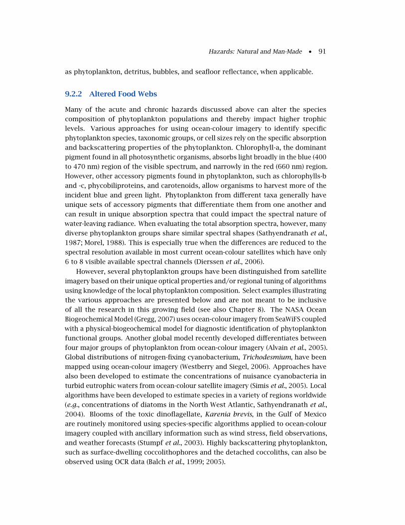
Hazards: Natural and Man-Made • 91
as phytoplankton, detritus, bubbles, and seafloor reflectance, when applicable.
9.2.2 Altered Food Webs
Many of the acute and chronic hazards discussed above can alter the species
composition of phytoplankton populations and thereby impact higher trophic
levels. Various approaches for using ocean-colour imagery to identify specific
phytoplankton species, taxonomic groups, or cell sizes rely on the specific absorption
and backscattering properties of the phytoplankton. Chlorophyll-a, the dominant
pigment found in all photosynthetic organisms, absorbs light broadly in the blue (400
to 470 nm) region of the visible spectrum, and narrowly in the red (660 nm) region.
However, other accessory pigments found in phytoplankton, such as chlorophylls-b
and -c, phycobiliproteins, and carotenoids, allow organisms to harvest more of the
incident blue and green light. Phytoplankton from different taxa generally have
unique sets of accessory pigments that differentiate them from one another and
can result in unique absorption spectra that could impact the spectral nature of
water-leaving radiance. When evaluating the total absorption spectra, however, many
diverse phytoplankton groups share similar spectral shapes (Sathyendranath et al.,
1987; Morel, 1988). This is especially true when the differences are reduced to the
spectral resolution available in most current ocean-colour satellites which have only
6 to 8 visible available spectral channels (Dierssen et al., 2006).
However, several phytoplankton groups have been distinguished from satellite
imagery based on their unique optical properties and/or regional tuning of algorithms
using knowledge of the local phytoplankton composition. Select examples illustrating
the various approaches are presented below and are not meant to be inclusive
of all the research in this growing field (see also Chapter 8). The NASA Ocean
Biogeochemical Model (Gregg, 2007) uses ocean-colour imagery from SeaWiFS coupled
with a physical-biogeochemical model for diagnostic identification of phytoplankton
functional groups. Another global model recently developed differentiates between
four major groups of phytoplankton from ocean-colour imagery (Alvain et al., 2005).
Global distributions of nitrogen-fixing cyanobacterium, Trichodesmium, have been
mapped using ocean-colour imagery (Westberry and Siegel, 2006). Approaches have
also been developed to estimate the concentrations of nuisance cyanobacteria in
turbid eutrophic waters from ocean-colour satellite imagery (Simis et al., 2005). Local
algorithms have been developed to estimate species in a variety of regions worldwide
(e.g., concentrations of diatoms in the North West Atlantic, Sathyendranath et al.,
2004). Blooms of the toxic dinoflagellate, Karenia brevis, in the Gulf of Mexico
are routinely monitored using species-specific algorithms applied to ocean-colour
imagery coupled with ancillary information such as wind stress, field observations,
and weather forecasts (Stumpf et al., 2003). Highly backscattering phytoplankton,
such as surface-dwelling coccolithophores and the detached coccoliths, can also be
observed using OCR data (Balch et al., 1999; 2005).

92 • Why Ocean Colour? The Societal Benefits of Ocean-Colour Technology
In natural communities, the cell size of the dominant phytoplankton organism,
varying from picoplankton (<2 µm), ultraplankton (2-5 µm), nanoplankton (5-20
µm), to microplankton (>20 µm), can explain over 80% of the variability of the
spectral shape of the phytoplankton absorption coefficient (Ciotti et al., 2002). Large
microplankton absorb less light per mg of chlorophyll than small picoplankon.
Correspondingly, recent efforts have been directed at estimating phytoplankton cell
size directly from ocean-colour imagery (Ciotti and Bricaud, 2006). Such an approach
can be useful in detecting shifts in ocean ecosystems from larger microplankton,
such as diatoms, to predominantly picoplankton, such as Prochlorococcus, which
would have significant implications for the trophic web.
Responses of coastal regions linked to terrestrial changes can also be observed
with ocean-colour imagery. For example, warming of the Eurasian landmass has
led to enhanced productivity in the water column (Goés et al., 2005). In a similarly
dramatic example, agricultural runoff from fields in Mexico was shown to stimulate
large phytoplankton blooms in the Gulf of California (Berman et al., 2005). Such
large blooms stimulated by terrestrial forces distant from the region can alter water
clarity, change the trophic structure of the water column, and potentially lead to
anoxic conditions.
9.2.3 Harmful Algal Blooms
Ocean-colour radiometry offers cost-effective, frequently acquired, synoptic data
pertaining to phytoplankton biomass in surface waters, and is thus of considerable
value in monitoring and better understanding harmful algal blooms (HABs). These
are an increasingly frequent occurrence in coastal waters around the globe, often
resulting in severe negative impacts to local marine ecosystems and communities, in
addition to commercial marine concerns such as aquaculture operations (Hallegraeff,
1993). Harmful impacts of algal blooms, often composed of a variety of dinoflagellate
species (Fig. 9.6), are associated primarily with the toxicity of some species present
in the algal assemblage, or the high biomass such blooms can achieve in highly
eutrophic systems. Upwelling systems provide dramatic examples of these impacts,
where collapse of high biomass blooms through natural causes such as nutrient
exhaustion can lead to hypoxic events and in extreme cases, the production of
hydrogen sulphide, causing extensive mortalities of marine organisms (Fig. 9.7).
Ocean-colour radiometry can play an important role in effective ecosystem
management with regard to HABs: routinely acquired synoptic data relating to
phytoplankton dynamics allows both a greater understanding of the variability of
HABs as ecologically prominent phenomena, in addition to a means of detecting and
monitoring blooms in real time (Ryan et al., 2002).
All phytoplankton are intimately connected to their physical environment and are
subject to horizontal transport. The ability to understand HAB growth and movement
in coastal systems depends fundamentally on understanding not only causative

Hazards: Natural and Man-Made • 93
Figure 9.6 The majority of harmful algal blooms are attributed to dinoflagellatespecies, and the harmful impacts are associated with either their highbiomass or toxic properties. Depicted in this figure are some of the bloom-forming dinoflagellates common in the Benguela upwelling system, includingAlexandrium catenella (2nd on top), Dinophysis fortii (3rd on top) and Dinophysisacuminata (2nd on bottom), three of the most common toxic species in theBenguela. (Image provided by Grant Pitcher, Marine and Coastal Management,South Africa).
biological processes and typical patterns of phytoplankton species succession,
but also the physical environment in which HABs occur. Time series of ocean-
colour products, in conjunction with other remotely-sensed data such as sea
surface temperature, can improve understanding of regional forcing and transport
mechanisms. Analyses such as these not only improve our understanding of why
and when HABs are likely to occur, but also greatly improve our ability to predict
HAB occurrence operationally (Stumpf et al., 2003; Pitcher and Weeks, 2006).
Natural resource managers and public health officials need better tools to detect
and monitor HAB events so that mitigation actions can be effectively taken. Bio-
optical systems, including remotely-sensed ocean-colour data, offer a cost-effective
means of obtaining real-time data relating to the algal assemblage using a variety
of platforms, sensor systems, and processing techniques ranging from standard
empirical products to the use of sophisticated analytical inversion algorithms (a
recent synopsis of available techniques can be found in Glen et al., 2004). Analytical
reflectance inversion algorithms in particular offer the ability to derive information
on the type of algal assemblage present in the water, in addition to gross algal
biomass (IOCCG, 2006). Such algorithms also allow the derivation of other water
constituents, such as sediment concentrations and algal degradation products, which
may be of utility in assessing environmental control mechanisms. An example of the
approach can be seen from MERIS images of southern Benguela (Fig. 9.8), showing

94 • Why Ocean Colour? The Societal Benefits of Ocean-Colour Technology
Figure 9.7 Many marine mortalities are attributed to harmful algal blooms andassociated with either hypoxic or toxic events. The above stranding of 2,000tons of rock lobster on the South African west coast was caused by decliningoxygen concentrations to below detectable levels following the decay of a bloomof the dinoflagellate Ceratium furca. (Credit: Grant Pitcher, MCM, South Africa).
the detection of the change of dominant assemblage during a high biomass bloom
event. In situ sampling confirmed that the dominant HAB species had changed from
the small dinoflagellate Prorocentrum triestinum to the large celled Ceratium furca.
The approach also offers a significant advantage in that it allows the derivation of
equivalent geophysical products from in situ, airborne, or space-based sensors. This
offers the ability to use analogous multi-platform derived data measured on a variety
of temporal and spatial scales, i.e., Eulerian high frequency mooring-derived data
and daily synoptic satellite-derived data.
There is a great need for satellite observations at higher spatial resolution to
monitor near-shore regions, estuaries and fjords where fish farms or shellfish beds
are frequently located. NASA’s MODIS-Aqua sensor has the capability to capture
data at both 250 m and 500 m spatial resolution, although only two of the 500 m
bands and one 250 m band have centre wavelengths in the visible spectrum. Shutler
et al. (2007) recently developed a dynamic atmospheric correction approach to use
these bands to retrieve chlorophyll. ESA’s MERIS sensor currently offers the best
capability with a 300 m resolution for all 15 wavebands, and 1-3 day revisit time.
Figure 9.9 shows a MERIS image of a bloom of harmful Karenia mikimotoi to the
east of the Orkney Isles, Scotland. MERIS 300-m resolution data are now available in
near-real-time via a rolling archive over Europe and North America, which should
enhance the use of ocean-colour data in near-shore environments.
Improving and expanding the forecasting capabilities offered by remote sensing
technologies will provide rapid and spatially-broad information. This information

Hazards: Natural and Man-Made • 95
Figure 9.8 Experimental analytical reflectance products showing the complexspatial distribution of a high biomass HAB event in the southern Benguela,and a change in the HAB assemblage in response to environmental conditions.Panels (a) and (b) show Chl-a concentrations approximately one week apart,while (c) and (d) depict the algal effective diameter, indicating a change to alarge-cell dominated assemblage in (d). (Credit: Image provided by StewartBernard, CSIR-NRE, South Africa, MERIS data provided by the European SpaceAgency).
will permit monitoring of the environmental conditions that promote HAB formation
as well as the tracking of HABs as they transit through a region. Making user-focussed
ocean colour and other remotely-sensed products more widely available and easy to
use is central to the more effective use of ocean colour for HAB applications. The
ChloroGIN programme (Chlorophyll Globally Integrated Network), under the auspices
of GEO (Group on Earth Observations) and GOOS (Global Ocean Observing System)
aims to play a key role in making HAB-related products more accessible to a wide
variety of users though web-based dissemination systems. Ocean-colour algorithm
development is also of considerable importance, as information on assemblage type
in addition to biomass are vital for HAB applications, and such research is ongoing
internationally.
Remote sensing has an important role to play in improving our understanding
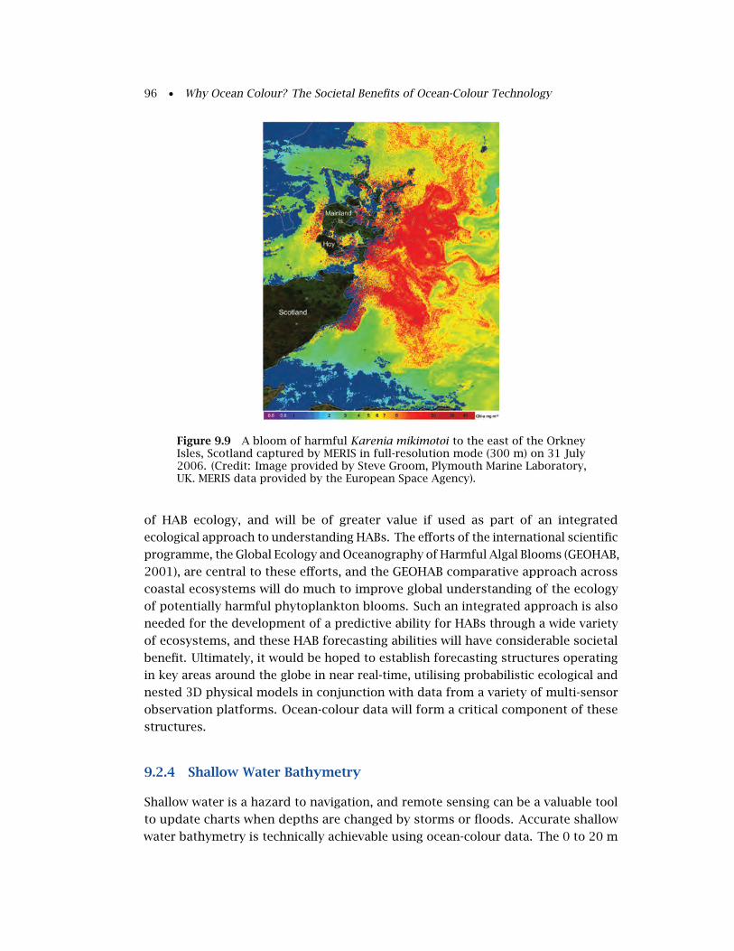
96 • Why Ocean Colour? The Societal Benefits of Ocean-Colour Technology
Figure 9.9 A bloom of harmful Karenia mikimotoi to the east of the OrkneyIsles, Scotland captured by MERIS in full-resolution mode (300 m) on 31 July2006. (Credit: Image provided by Steve Groom, Plymouth Marine Laboratory,UK. MERIS data provided by the European Space Agency).
of HAB ecology, and will be of greater value if used as part of an integrated
ecological approach to understanding HABs. The efforts of the international scientific
programme, the Global Ecology and Oceanography of Harmful Algal Blooms (GEOHAB,
2001), are central to these efforts, and the GEOHAB comparative approach across
coastal ecosystems will do much to improve global understanding of the ecology
of potentially harmful phytoplankton blooms. Such an integrated approach is also
needed for the development of a predictive ability for HABs through a wide variety
of ecosystems, and these HAB forecasting abilities will have considerable societal
benefit. Ultimately, it would be hoped to establish forecasting structures operating
in key areas around the globe in near real-time, utilising probabilistic ecological and
nested 3D physical models in conjunction with data from a variety of multi-sensor
observation platforms. Ocean-colour data will form a critical component of these
structures.
9.2.4 Shallow Water Bathymetry
Shallow water is a hazard to navigation, and remote sensing can be a valuable tool
to update charts when depths are changed by storms or floods. Accurate shallow
water bathymetry is technically achievable using ocean-colour data. The 0 to 20 m

Hazards: Natural and Man-Made • 97
water depth is frequently lacking in most coastal databases because hydrographic
survey vessels do not navigate in these near-shore regions. Remote sensing has
the capability to monitor coastal benthic features and associated water column
properties, using sensors that have spatial resolution of few metres (e.g. SPOT-HRV,
Landsat TM). These sensors have a limited set of wavelengths in the visible, but
the spectral contrast between various bottom structures can be used to construct
classification algorithms based on differential reflectance (Andréfouët et al., 2001;
Hochberg et al., 2003).
9.2.5 Benthic Habitat Loss
Ocean-colour remote sensing is an emerging tool for characterizing changes to
benthic habitats in water where the reflectance of the seafloor can be observed
or detected from above the water’s surface, often referred to as ‘optically-shallow
water’. Traditionally, the products obtained from ocean-colour satellites have focused
on unicellular phytoplankton in the surface layers of the world’s oceans, but the
imagery can also be used to characterize seafloor reflectance and hence bottom
type in optically-shallow water. Understanding of benthic optical properties and
light propagation in optically-shallow waters has advanced significantly in recent
years and many algorithms have been developed and applied to identify benthic
ecosystems. By definition, benthic environments in optically-shallow waters are
within the photic zone and receive enough sunlight to support photosynthesis
by seagrasses, macroalgae, kelps, and even zooxanthellae living symbiotically with
corals. Ocean-colour remote sensing offers a cost-effective approach for mapping and
potentially quantifying benthic substrate that is highly repeatable and cost-effective
for detecting large scale changes in the benthos, particular in large homogenous
regions (Dekker et al., 2006).
Stumpf et al. (1999) used AVHRR data, with only one visible channel (580-680
nm) to investigate water column turbidity events and potential presence/absence of
seagrasses. Single channel radiometers provide limited information that can be used
to uncouple water column constituents (e.g., phytoplankton and sediments) from
bottom albedo. Regions of low reflectance were associated with dense seagrasses
and/or phytoplankton blooms, while regions of high reflectance were either turbid
waters or optically shallow waters with highly reflective bottoms.
Remote sensing has also been used to document resilience in benthic features
to hurricanes and other large scale disturbances. Seagrass distributions observed
with high resolution imagery from the Portable Hyperspectral Imager for Low Light
Spectroscopy (Ocean PHILLS) were analyzed in the eastern portion of the Bahamas
Banks near Lee Stocking Island. Meadows varied from sparse (leaf area index
<0.5) to very dense (leaf area index >2) over metre scales (Dierssen et al., 2003).
Analysis of airborne imagery was analyzed before and after Hurricane Floyd passed
directly across the study region. Although this storm inflicted significant damage to
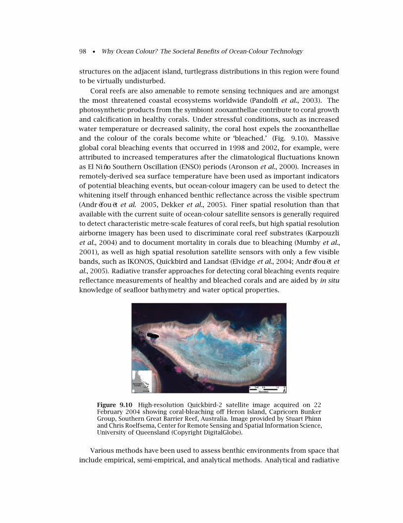
98 • Why Ocean Colour? The Societal Benefits of Ocean-Colour Technology
structures on the adjacent island, turtlegrass distributions in this region were found
to be virtually undisturbed.
Coral reefs are also amenable to remote sensing techniques and are amongst
the most threatened coastal ecosystems worldwide (Pandolfi et al., 2003). The
photosynthetic products from the symbiont zooxanthellae contribute to coral growth
and calcification in healthy corals. Under stressful conditions, such as increased
water temperature or decreased salinity, the coral host expels the zooxanthellae
and the colour of the corals become white or ‘bleached.’ (Fig. 9.10). Massive
global coral bleaching events that occurred in 1998 and 2002, for example, were
attributed to increased temperatures after the climatological fluctuations known
as El Niño Southern Oscillation (ENSO) periods (Aronson et al., 2000). Increases in
remotely-derived sea surface temperature have been used as important indicators
of potential bleaching events, but ocean-colour imagery can be used to detect the
whitening itself through enhanced benthic reflectance across the visible spectrum
(Andréfouët et al. 2005, Dekker et al., 2005). Finer spatial resolution than that
available with the current suite of ocean-colour satellite sensors is generally required
to detect characteristic metre-scale features of coral reefs, but high spatial resolution
airborne imagery has been used to discriminate coral reef substrates (Karpouzli
et al., 2004) and to document mortality in corals due to bleaching (Mumby et al.,
2001), as well as high spatial resolution satellite sensors with only a few visible
bands, such as IKONOS, Quickbird and Landsat (Elvidge et al., 2004; Andréfouët et
al., 2005). Radiative transfer approaches for detecting coral bleaching events require
reflectance measurements of healthy and bleached corals and are aided by in situ
knowledge of seafloor bathymetry and water optical properties.
Figure 9.10 High-resolution Quickbird-2 satellite image acquired on 22February 2004 showing coral-bleaching off Heron Island, Capricorn BunkerGroup, Southern Great Barrier Reef, Australia. Image provided by Stuart Phinnand Chris Roelfsema, Center for Remote Sensing and Spatial Information Science,University of Queensland (Copyright DigitalGlobe).
Various methods have been used to assess benthic environments from space that
include empirical, semi-empirical, and analytical methods. Analytical and radiative
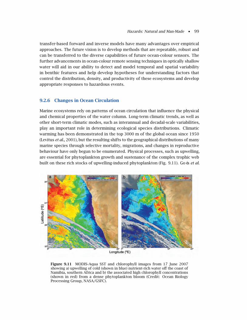
Hazards: Natural and Man-Made • 99
transfer-based forward and inverse models have many advantages over empirical
approaches. The future vision is to develop methods that are repeatable, robust and
can be transferred to the diverse capabilities of future ocean-colour sensors. The
further advancements in ocean-colour remote sensing techniques in optically shallow
water will aid in our ability to detect and model temporal and spatial variability
in benthic features and help develop hypotheses for understanding factors that
control the distribution, density, and productivity of these ecosystems and develop
appropriate responses to hazardous events.
9.2.6 Changes in Ocean Circulation
Marine ecosystems rely on patterns of ocean circulation that influence the physical
and chemical properties of the water column. Long-term climatic trends, as well as
other short-term climatic modes, such as interannual and decadal-scale variabilities,
play an important role in determining ecological species distributions. Climatic
warming has been demonstrated in the top 3000 m of the global ocean since 1950
(Levitus et al., 2001), but the resulting shifts to the geographical distributions of many
marine species through selective mortality, migrations, and changes in reproductive
behaviour have only begun to be enumerated. Physical processes, such as upwelling,
are essential for phytoplankton growth and sustenance of the complex trophic web
built on these rich stocks of upwelling-induced phytoplankton (Fig. 9.11). Goés et al.
Figure 9.11 MODIS-Aqua SST and chlorophyll images from 17 June 2007showing a) upwelling of cold (shown in blue) nutrient-rich water off the coast ofNamibia, southern Africa and b) the associated high chlorophyll concentrations(shown in red) from a dense phytoplankton bloom (Credit: Ocean BiologyProcessing Group, NASA/GSFC).

100 • Why Ocean Colour? The Societal Benefits of Ocean-Colour Technology
(2005) documented how the warming Eurasian landmass has escalated the intensity
of summer monsoon winds and strengthened upwelling in the western Arabian
Sea. This coupled atmosphere-land-ocean phenomenon was linked to enhanced
satellite-derived chlorophyll concentrations in the surface waters of the Arabian Sea
using imagery from both the ADEOS-1 Ocean Colour Temperature Sensor (OCTS,
Japan) and SeaWiFS. Regional changes in productivity, such as this example, can lead
to altered fish stocks, oxygen concentrations in the water, and the significant shifts
in the trophic status of these waters.
Moreover, the timing, onset, and intensity of coastal upwelling is critical for
species whose life histories are closely tuned to the annual cycle. Some studies have
suggested that rising ocean temperatures have contributed to decreased upwelling
in certain regions. In turn, the dwindling plankton populations have significant
influences on the marine ecosystem, including seabird communities (Hyrenbach and
Veit, 2003). Marine bird concentrations have been shown to be positively correlated
to primary productivity in the water column. Upwelling regions, such as Point
Conception, California, appear to be important ‘hot spots’ of sustained primary
productivity and marine bird concentrations (Yen et al., 2006). For example, in 2005
coastal ocean temperatures were 2 to 5 degrees above normal throughout the west
coast of the United States and Canada, apparently caused by a lack of upwelling that
brings cold, nutrient-rich water to the surface. These warmer ocean temperatures
were linked to decreased fish stocks (e.g., salmon and rockfish) and decreased nesting
success and mortality of seabirds (e.g., cormorants and auklets) which require high
marine productivity in the spring months for successful breeding. These shifts in
upwelling are not only observed in North America, but have been observed globally
including Antarctica and Europe.
9.3 Future Directions
As demonstrated above, ocean-colour imagery has been used successfully to
document hazardous events and to determine the impacts of acute and chronic
hazards on the oceans. Such imagery is currently being used to track the course
of tropical storms and hurricanes, document coastal erosion and sediment re-
suspension events, harmful algal blooms, and to identify changes to benthic habitats
and the trophic food web throughout the world’s seas. Many of these methods
are qualitative and show only those impacts that can be observed visually from a
true colour image, such as the apparent extent and duration of a sediment plume.
However, the considerable research into the optical properties of the water column
and benthos, coupled with radiative transfer modelling, has led to the development
of more advanced methods for characterizing these changing environments. The
use of ocean-colour imagery to assess hazards is an emerging field. For example,
further research is needed to integrate the various relevant measurements required

Hazards: Natural and Man-Made • 101
to understand intense algal bloom development and the propensity of these blooms
to produce toxins. As storm surges erode coastlines, we also need better methods
to identify the amount of eroded material and depth of flood waters in inland areas.
Modelling flood water properties will require an understanding of the water’s optical
properties.
Quantifying hazardous events and changes to the world’s ocean resources
requires higher temporal, spatial, and spectral resolution imagery than currently
available. Analytical and semi-analytical methods for evaluating this imagery will
require that both the magnitude and spectral shape of the retrieved sea surface
reflectance are accurate. Hence, new atmospheric correction approaches must
be developed that handle significant amounts of near-infrared reflectance and
absorbing aerosols common to the coastal zone. Research is also needed to develop
algorithms that are not merely site-specific empirical regressions, but which can
actually determine the quantity and composition within the surface waters and on
the seafloor. Integrated modelling and data assimilation efforts will be required to
tie together in situ measurements and a variety of remote-sensing data including sea
surface temperature and bathymetry.

102 • Why Ocean Colour? The Societal Benefits of Ocean-Colour Technology

Chapter 10
Ocean Colour and Climate Change
Nick Hoepffner, Cara Wilson and Samantha Lavender
The longest currently-operating ocean-colour sensor (SeaWiFS) was launched in 1997,
so it is not possible to detect decade-scale variability using SeaWiFS data alone. Newer
and overlapping missions such as MODIS-Aqua and MERIS (launched in 2002) will
hopefully ensure unbroken observations and provide global ocean-colour products
up to 2012, with an increased spatial coverage. In the meantime, long-term changes
can be observed by comparing climatological SeaWiFS/ MODIS/ MERIS data against
data from the Coastal Zone Colour Scanner (CZCS), which operated between 1979 and
1985. The following section focuses on a few recent applications using these ocean-
colour time-series to detect long-term trends in marine biology due to climate change.
Notwithstanding the current limitation of ocean colour in obtaining a data set with
a time frame of several decades, ocean colour is identified as an Essential Climate
Variable (ECV) within the Global Climate Observing System (GCOS) action plan to
support the United Nations Framework Convention on Climate Change (UNFCCC)
and the work carried out by the Intergovernmental Panel on Climate Change (IPCC),
representing a unique synoptic-scale view of the pelagic ecosystem. As such, it is
absolutely essential to avoid any temporal gaps in the ocean-colour record, which
has already suffered considerably from the ∼10-year gap between the CZCS and
SeaWiFS missions. Moreover, the provision of a single and consistent data stream
of ocean-colour products from multi-platform devices would optimize the use of
ocean-colour radiometry (OCR) data in climate research.
10.1 Long-Term Changes in Phytoplankton Biomass
Gregg et al. (2002) and Antoine et al. (2005) conducted a comprehensive re-analysis
of CZCS data using similar methods and algorithms (as far as possible) to those used
for current sensors, such that comparison of ocean-colour data sets from both eras
could be achieved with a reasonable level of confidence. This analysis of decadal
changes between CZCS and SeaWiFS data sets yielded an overall increase of 22% in
the global ocean chlorophyll concentration (Antoine et al. 2005). Using only 6 years
of SeaWiFS data, Gregg et al. (2005) also observed a slight increase in global ocean
103

104 • Why Ocean Colour? The Societal Benefits of Ocean-Colour Technology
chlorophyll concentration (4.1%).
Although the global average ocean chlorophyll concentration is observed to be
increasing, some regions of the ocean show a decrease. For the oceanic carbon cycle
and ecosystem assessment it is important to understand where these changes are
occurring. The largest positive changes between CZCS and SeaWiFS data sets are
observed in the inter-tropical regions, whereas the oligotrophic gyres are becoming
even more impoverished (Antoine et al., 2005). Using a 9-year time series of SeaWiFS
data, Polovina et al. (2008) demonstrated that in the North and South Pacific
and North and South Atlantic, outside the equatorial zone, areas of low surface
chlorophyll waters have expanded at average annual rates from 0.8 to 4.3% yr−1.
According to the authors, the expansion of low chlorophyll waters is consistent
with global warming scenarios, implying increased vertical stratification in the mid-
latitudes. The rates of expansion as observed with satellite data, however, greatly
exceeds recent model predictions. Vantrepotte and Mélin (2008, subm.) also reported
a decline in chlorophyll concentrations in the subtropical gyres at rates ranging from
1 to 5% per year, based on a decade of SeaWiFS data (1997-2007, Fig. 10.1).
Figure 10.1 Linear changes in SeaWiFS-derived chlorophyll concentration fromSeptember 1997 to December 2007 (in % per year). Only the pixels for whicha significant linear trend was detected, are reported (p < 0.05, Student-t test).(Image provided by Vincent Vantrepotte, Joint Research Centre, EC).
Positive changes, i.e. increases in chlorophyll concentrations, seem to be confined
in coastal regions and upwelling areas. Several lines of evidence show an increasing
strength of the seasonal upwelling in different systems over several decades, using
other data sources (Bakun 1990; Snyder et al. 2003) and would explain the subsequent
rise in chlorophyll in these regions. Likewise, using 11-years of data from SeaWiFs
and its predecessor OCTS, Kahru and Mitchell (2008) found that bloom magnitudes
have increased significantly in eastern boundary upwelling systems, as well as in a

Ocean Colour and Climate Change • 105
number of areas known to be sensitive to eutrophication (e.g. enclosed and semi-
enclosed basins, outflow areas of large rivers). Some of the observed trends in bloom
magnitude could be attributable to the strong El Niño of 1997-98 at the start of the
time series. However, bloom magnitudes have increased in many areas even after
this event.
Long-term changes in phytoplankton biomass could be reflected in the global
ocean primary production and the entire carbon cycle. Comparing the CZCS record
with 6 years of SeaWiFS data, Gregg et al. (2003) demonstrated a slight decrease of
6.3% in the global marine primary production, most of the decline being observed
at mid- to high-latitudes. In contrast, low latitude and equatorial areas showed an
increase in primary production between the CZCS and SeaWiFS eras. Using 9 years
of SeaWiFS imagery (1997-2006), Behrenfeld et al. (2006) showed a decrease in net
primary production over the years after an initial boost in 1998 due to the El Niño
event.
Despite the different methodologies used, a certain level of consistency emerges
from these OCR investigations, indicating that phytoplankton chlorophyll and
primary production in large regions of the ocean (mid-latitude gyres) are decreasing
over a multi-year period. Considering the limited ocean colour time-series being
used (mainly SeaWiFS era), any interpretation of the changes as representative of
longer term trends possibly linked to global warming would be speculative. Yoder
and Kennelly (2003) documented a significant relationship between the inter-annual
variability of chlorophyll and the large ENSO (El Niño Southern Oscillation) event
which took place in 1997, and had global impacts for many years. Behrenfeld et
al. (2006) also underline the striking correspondence between changes in primary
production and a Multivariate ENSO Index, which would relate observed trends
in chlorophyll and primary production to climate variability, rather than climate
change.
10.2 Fisheries and Climate
The 1997/98 El Niño was one of the strongest ENSO events of the century. Ocean
colour satellite data, in synergy with data from an extensive array of moorings
across the equatorial Pacific, have contributed enormously to our understanding of
ENSO dynamics and their ecosystem impacts. Deepening of the thermocline, and
cessation of upwelling along the equator and in the coastal ecosystems lowers ocean
productivity and causes significant depression of the anchovy fisheries of Peru and
Chile (Alamo and Bouchon, 1987; Escribano et al., 2004). However, other species are
positively impacted by El Niño, for example increases are observed in the biomass of
sardine and mackerel (Bakun and Broad, 2003; Niquen and Bouchon, 2004). Satellite
ocean-colour data have demonstrated that the effects of El Niño are not constrained
to just the equatorial and coastal upwelling regions, but extend throughout most

106 • Why Ocean Colour? The Societal Benefits of Ocean-Colour Technology
of the Pacific Ocean. For example during the 1997/98 event the Transitional Zone
Chlorophyll Front (TZCF) was shifted ∼5◦ south of its regular position (Bograd et al.,
2004), and lower chlorophyll values occurred across most of the subtropical Pacific
(Wilson and Adamec, 2001).
On a longer time scale, the present wintertime position of the TZCF in the Pacific,
as observed with SeaWiFS data set, is about 5◦ further north than it was during the
CZCS time period (Fig. 10.2). This shift has also been seen in SST data used as a proxy
for the TZCF (Bograd et al., 2004). Data from the CZCS and SeaWiFS sensors have
also been used to identify regions of the ocean which have experienced significant
changes in the concentration of chlorophyll and rate of primary productivity in the
past twenty years (Gregg and Conkright, 2002; Gregg et al., 2003).
Figure 10.2 Interannual variation in the position of the TZCF indicated by themean January position from CZCS data (1979-1985) in purple, and from SeaWiFSdata (1998-2004) in red. The winter TZCF is presently ∼5◦ further north fromits position during the CZCS era. (Credit: Cara Wilson, unpublished data)
There is significant long-term temporal variability in fish stocks, and for over 150
years scientists have been trying to differentiate the effects of interannual variability,
overfishing and long-term changes such as regime shifts, which are characterized by
relatively rapid changes in the baseline abundances of both exploited and unexploited
species (Polovina, 2005). Long-term variations in ecosystems often follow trends
or patterns also observed in ocean and atmosphere properties (Mantua et al., 1997;
Hare and Mantua, 2000; Peterson and Schwing, 2003). For example, a shift in the
North Pacific in the 1970’s between a shrimp-dominated ecosystem to one populated
primarily by several species of bottom-dwelling groundfish species coincided with
a regional change from a cool to a warm climate (Botsford et al., 1997; Anderson
and Piatt, 1999; Fig. 10.3). Although similar phenomena have been seen for many
different stocks, and in all ocean basins, the mechanisms that link large-scale ocean
and atmosphere dynamics to changes in population abundances are not always
clear (Botsford et al., 1997; Baumann, 1998) and the relationships are not always
constant over time (Solow, 2002). Ecosystem changes related to regime shifts are not
in themselves harmful to the ecosystems as a whole (Bakun and Broad, 2003), but to
maintain sustainability, management practices must be flexible enough to recognize
and accommodate them (Polovina, 2005). Chassot et al. (2007) used satellite-derived
primary productivity data together with catch data from European seas for the

Ocean Colour and Climate Change • 107
period 1998 to 2004, and found significant positive relationships between primary
production and yield, suggesting a strong linkage between marine productivity and
fisheries production. This is relevant in the context of climate change, because
variations in primary production linked to global warming could strongly modify
fisheries production in the future.
Figure 10.3 Changes in the composition of small-mesh trawl catches in theGulf of Alaska (GOA) between 1953 and 1997, in relation to climate indices.Chart data expressed as normalized anomalies (NPPI: North Pacific PressureIndex; BC: British Columbia), and shown visually in photos of small-mesh bottomtrawl surveys in Pavlov Bay, Alaska (right). Figures adapted from Anderson andPiatt (1999) and Botsford et al. (1997). Reprinted with permission from AAAS.
One of the current limitations of satellite data is the relatively short time-span
of the data series. For fisheries applications it is crucial that climate-quality records
of ocean colour be maintained so that existing satellite records will be able to serve
as a benchmark against which to gauge future changes.
10.3 Toward a Long-Term and Consistent Ocean-Colour TimeSeries
To examine long-term changes in ocean colour for climate monitoring purposes,
ocean-colour data sets need to be based on individual sensors with a significant
historical archive, or a time-series of several overlapping, well-calibrated sensors that

108 • Why Ocean Colour? The Societal Benefits of Ocean-Colour Technology
can be combined to produce a consistent, well-calibrated merged data set. Individual
sensors typically have a nominal lifetime of 5 years, but in reality their operating
period can be much shorter (e.g. OCTS which provided data for 8 months prior
to a power failure), or longer (e.g. SeaWiFS currently in its 11th year of activity).
Currently, no operational satellite ocean-colour missions are designed to provide
multi-decadal observations of the marine biological field, such as the NOAA-AVHRR
series for measurement of sea surface temperature. However, ESA’s Sentinel-3
series of operational satellites, the first of which is scheduled for launch in 2012,
are designed to provide an uninterrupted flow of robust global data products. At
the moment, the ocean-colour community has to rely on a number of individual
missions launched by various space agencies, with radiometric sensors that differ in
their technical specifications. Multiple overlapping missions, such as the current
SeaWiFS, MODIS and MERIS missions, have the advantage of increasing the spatial
coverage of the global ocean, which is more limited with a single sensor due to
the effects of sun-glint and clouds (IOCCG 1999). The challenge is to maximize
the information available by combining data from individual sensors, such that a
reasonably consistent and well calibrated data stream of ocean-colour products can
be generated independently of sensor characteristics and satellite orbital schemes.
NASA’s Sensor Intercomparison for Marine Biological and Interdisciplinary Ocean
Studies (SIMBIOS) Program was conceived in 1994 to examine the technical challenges
of combining ocean-colour data from an array of individual missions to form
consistent and accurate global bio-optical time-series products. A specific objective
of the program was to develop appropriate methods for merging data from sensors
with different viewing geometries, resolution (spectral, spatial and temporal), and
other radiometric features. Several merged ocean-colour data sets have become
available in recent years:
v NASA OBPG merged Chl-a data set based on SeaWiFS and MODIS-Aqua,
v NASA REASoN merged Chl-a, Colour Dissolved Material (CDM) and particulate
backscattering (bbp) data sets based on SeaWiFS and MODIS-Aqua,
v ESA DUE GlobColour multi-parameter (19 variables) data set based on SeaWiFS,
MERIS and MODIS.
The merging of data from individual sensors not only provides a long time-series,
but also increases the temporal coverage (see Table 10.1) and error characterisation
of the final data set. The averaged daily coverage by individual sensors ranges from
∼8% for MERIS to ∼16% for SeaWiFS. The combination of two sensors increases the
global ocean coverage to ∼20-25% per day, and to ∼30% per day with the combination
of three sensors (IOCCG, 1999).
The GlobColour Project was initiated and funded by the ESA Data User Element
(DUE) Programme in 2005 to develop a satellite-based ocean-colour data set to
support global carbon-cycle research, and to satisfy the scientific requirement for a
long time series of consistently calibrated global ocean-colour information with the

Ocean Colour and Climate Change • 109
Table 10.1 Ocean-colour sensor average daily coverage plus standard deviation for 2003(produced by Stephane Maritorena and based on the GlobColour Chl-a data).
Sensor(s) Coverage (%) StandardDeviation (%)
SeaWiFS 16.65 2.01MODIS-Aqua 13.76 1.15MERIS 8.51 1.48SeaWiFS/MODIS-Aqua 24.22 1.94SeaWiFS/MERIS 22.24 2.40MODIS-Aqua/MERIS 19.92 1.74SeaWiFS/MODIS-Aqua/MERIS 28.85 2.24
best possible spatial coverage. This was achieved by merging data from the SeaWiFS,
MODIS-Aqua and MERIS missions. The project provides global daily, 8-day, and
monthly merged data products at 4.6-km resolution for the time period 1997-2007,
and is freely available to the scientific user community (http://www.globcolour.info).

110 • Why Ocean Colour? The Societal Benefits of Ocean-Colour Technology

Chapter 11
Future Perspectives
James Yoder, Paula Bontempi, Paul DiGiacomo, Hiroshi Murakami, PeterRegner, Gordon Campbell and Simon Pinnock
11.1 Current Situation and Future Directions
Today we find ourselves standing on the threshold of profound breakthroughs in
ocean biological sciences. By virtue of the opportunities provided by the first
generation of ocean-colour satellite missions during the past decade, we have
realised major advances in our ability to resolve multiple in-water constituents
from remote sensing data, related these to key components and processes within
ocean ecosystems, and integrated this new information into advanced prognostic
models. Over this same period, we have also seen major technological developments
that can enable the new measurements necessary to address the remaining top
priority questions in environmental policy and ocean science.
The focus on science in service of societal needs is supporting the elaboration
of extended requirements among environmental protection and other operational
agencies throughout the world for marine environment monitoring, as well as putting
structures in place for enhanced exchange of marine information. Furthermore,
these operational communities acknowledge a critical reliance on continued research
to improve understanding of oceanic processes and their interaction with our health
and well-being. At the same time, commercial operators are increasingly affected
by environmental considerations and are adopting more innovative techniques to
collect, process and analyse the information necessary to support safe, efficient and
sustainable commercial practices.
As a result, a wide range of user communities have ambitious plans to use
satellite ocean-colour radiometry (OCR) for research, operational and commercial
applications. Space agencies are responding to these evolving requirements with
a set of OCR mission scenarios. In this chapter we consider the factors driving
increased demand for ocean-colour radiance measurements, the responses from the
space community and the technical issues to be addressed over the coming years
to ensure that the advances fostered by the ocean-colour community over the last
decade continue.
111
112 • Why Ocean Colour? The Societal Benefits of Ocean-Colour Technology
11.2 Evolving Needs for OCR Measurements
The research, operational and commercial user communities each have very different
requirements for ocean-colour derived information over the coming years.
11.2.1 Research Challenges in Ocean Colour
Of key importance in a world with a changing climate is a better understanding of the
Earth System. For example, the key research challenges in relation to ocean-colour
radiometry measurements, as elaborated by ESA in consultation with a group of
leading international Earth Scientists, and which are consistent with the science
goals of the other space agencies, include:
v quantifying the interaction between variability in ocean dynamics, thermohaline
circulation, sea level and climate;
v quantifying primary production and its role in the ocean carbon cycle;
v understanding physical and bio-chemical air/sea interaction processes;
v understanding internal waves and mesoscale variability in the ocean, its
relevance for heat and energy transport and its influence on primary
production;
v quantifying marine-ecosystem variability and its natural and anthropogenic
physical, biological and geochemical forcing;
v understanding land/ocean interactions in terms of natural and anthropogenic
forcing;
v providing reliable model and data-based assessments and predictions of past,
present and future states of the ocean.
Research users are particularly interested in using ocean-colour imagery to help
detect and quantify the response of coastal and marine ecosystems to climate
change. Plankton are good indicators of climate change and documenting the timing,
magnitude and distribution of changes in their biomass and productivity on regional
to global scales over an extended time period offers a unique tool to monitor and
assess the effects of climate change on the aquatic ecosystem. This will likewise have
significant societal impacts and benefits associated with improved understanding
and insights gained from research.
11.2.2 Operational Use of OCR Data
Operational agencies responsible for managing society’s use of ocean and coastal
ecosystems, sustaining natural resources, protecting public health and ensuring
safe navigation are increasingly adopting ocean-colour derived information services
for routine monitoring and assessment tasks, and to help fulfil the mandate to
optimise use and protection of coastal and ocean resources. In Europe, for example,
the Global Monitoring for Environment and Security (GMES) initiative has fostered

Future Perspectives • 113
strong user acceptance of the operational use of ocean-colour data for water quality
monitoring. At the same time, new policies such as the Water Framework Directive
and the Marine Environment Strategy drive operational users to adapt their routine
monitoring programmes within the budgets available, and in such situations the cost-
effectiveness of satellite-based ocean-colour information is increasingly recognised.
This creates a parallel set of challenges to be addressed. Greater integration of
ocean-colour derived information into a wider operational monitoring and analysis
will drive requirements on spatial and radiometric resolution, data continuity, quality
control and validation in complex coastal environments.
Satellite ocean-colour data represent a powerful tool to assess the effectiveness
of policies and practices and support their application and enforcement. For
example, implementing ecosystem-based approaches to management with associated
integrated ecosystem assessments will increasingly rely on routine and synoptic
measurement of aquatic biological activity via satellite remote sensing. Improved
satellite OCR data and products will support a more timely and effective decision
making process, and enhance the ability of operational agencies to optimally manage
and protect the marine and coastal environment.
In the USA, Federal and state agencies share coastal ocean protection and man-
agement responsibilities including fisheries management, water quality monitoring,
protection of marine sanctuaries and marine mammal habitats, and assessing storm
event effects. These management responsibilities require an improved understanding
of context and change through time and space. This requires inter-calibration of
ocean-colour sensors and calibration to provide stable time series. Calibration and
Validation (Cal/Val) are therefore key activities for satellite remote sensing of ocean
optical, biological and biogeochemical properties in support of both research and
operations/applications, and will require an even greater focus in the future in the
context of virtual ocean-colour constellations and associated data exchange.
Beyond routine water quality and general ecosystem health and productivity
assessments, operational uses of satellite ocean-colour data will continue to grow
and include new and improved developments and applications in support of user
needs. Some potential new operational applications include:
v Creation of habitat suitability maps - establishing boundaries of marine
sanctuaries; managing commercially and recreationally important living marine
resources; directing in situ sampling efforts, and locating targeted organisms
such as Harmful Algal Blooms (HABs).
v Ecological prediction - forecasting year-class survival or growth rate of a
species based on the timing of the spring phytoplankton bloom; initialising
and validating results of numerical ecological models; improving ecological
forecasts through data assimilation; and nowcasting or forecasting the fate
and transport of pollutants and pathogens.
v Extended use for climate change and impact assessments - to better estimate

114 • Why Ocean Colour? The Societal Benefits of Ocean-Colour Technology
the spatio-temporal distribution of the air-sea CO2 flux and ocean acidification,
especially in the coastal zone where riverine inputs and productive filaments
can degrade the accuracy of estimates based only on sea surface temperature
and scatterometer-derived wind speeds; providing data on the long term
changes of surface biomass in response to climate change and other human
activities.
Finally, new and improved operational products will benefit from the continued
infusion, transition and integration of research and technology developments into
operational practices.
11.2.3 Commercial Use of OCR Data
Commercial operators are also realising the value of ocean-colour derived infor-
mation, and its utilisation among private sector customers is expected to increase
significantly over the coming years due to a greater demand for marine environment
information and high sensitivity to the cost effectiveness of the different data
gathering approaches. The aquaculture industry in Europe and South America is
probably the most advanced private sector user of ocean colour but at present this
is for relatively simple products (e.g. detection of algal blooms). In parallel with
the expansion of this industry, the demands for information are also growing. The
ocean-colour community has the opportunity to respond with new products such
as water mass delineation (e.g. to provide warnings of strong salinity variations,
oxygen concentration and the presence of harmful jelly fish), environmental impact
assessment and improved characterisation of algal bloom events. In addition to
aquaculture, commercial tour operators and sport fishing, marine engineers and
shipping operators are all demonstrating increased interest in the commercial use
of ocean-colour derived information such as transparency, sediment concentration
and chlorophyll concentration. One of the main evolution requirements from the
commercial sector is a robust capability to extract information close to the coast in
complex optical and geographic environments (e.g. high sediment loads, fjords and
estuaries, coral reefs).
11.3 Technical Developments for Wider OCR Utilization
The different user groups are setting strong challenges for the ocean-colour
community. For example, biological and ecosystem modelling requires quantification
of variables which are not yet calculated from ocean-colour radiometry measurements.
The lack of these data imposes constraints on model development and validation.
The response from the ocean-colour community may be improved algorithms for
processing existing data, enhanced data assimilation, new mission concepts, new
instruments and new infrastructure for enhanced data exchange. The ocean-science

Future Perspectives • 115
community also has significant expectations for the contribution of ocean colour as
a unique data stream for assimilation into coupled physical-biogeochemical models
and in support to the Global Climate Observing System (GCOS) Implementation Plan
as an Essential Climate Variable.
Research and operational users investigating and monitoring coastal and inland
waters require observations with improved spatial, temporal and spectral resolution
and coverage. In addition, there is a continuous requirement from the operational
user community for improved reliability of measurements and the capacity to extract
new parameters in optically complex, highly variable coastal areas. To respond
effectively, the ocean-colour community must develop new or improved capabilities
in at least the following key areas:
v separation of in-water constituents (e.g., organic and inorganic substances) in
global waters, which requires advanced corrections for atmospheric effects
on satellite ocean measurements as well as new, advanced algorithms for
characterising the parameters of interest;
v resolution of coastal phenomena and mapping of coastal habitats using high
temporal and spatial resolution measurements;
v active assessments of plant physiology and the function of different groups of
plants in aquatic ecosystems; and
v determining environmental variability of the surface ocean, including the depth
of the mixed layer.
At instrument level, the engineering focus must be on enhanced spatial and
spectral resolution while the space agencies together can ensure improved temporal
resolution.
Improved Spatial Resolution (200 - 300 m): Higher spatial resolution can provide
improved measurements for estuaries, bays and lakes, which are often used for
aquaculture applications, and can potentially also provide information for coral
reef and other near-shore ecosystems that are currently poorly resolved. Further,
finer spatial resolution ocean-colour data will improve the capability to track ocean
features and processes that influence migration, feeding, spawning and recruitment
of commercially important fish populations and many protected species. Clearly
this will also improve water quality monitoring and assessments through enhanced
detection of (harmful) algal blooms, freshwater run-off (often containing pollutants
and pathogens) and other phenomena and processes of interest.
Improved Spectral Resolution: River run off, suspended sediments, coloured
dissolved organic matter, large phytoplankton blooms and bottom reflectance in
shallow water all add to the optical complexity of coastal waters. Research has
shown that additional bands in the infrared and short wave infrared (SWIR) can
improve atmospheric correction, while additional bands in the red to near infrared
can aid identification of phytoplankton. Bands at the "red edge" from 680 to 709
nm have been used in methods to detect harmful algal blooms and the distribution

116 • Why Ocean Colour? The Societal Benefits of Ocean-Colour Technology
of Sargassum, while narrow spectral bands centered around 665 nm and 680 nm
are frequently used to measure the height of the chlorophyll-a fluorescence peak.
SWIR bands in particular are needed for turbid coastal waters. Additional ultraviolet
bands (UV) show potential for improving atmospheric correction and phytoplankton
discrimination, and also for better quantifying ocean organic and inorganic materials.
In the coastal regions, aerosol vertical profile information is needed, e.g. data from
the CALIPSO measurements. Most current and planned sensors do not measure in
enough different wavelengths to optimise separation of components in optically-
complex waters and none provide enough bands for optimal atmospheric correction.
Higher spectral resolution (narrower/more bands) and greater spectral coverage,
from the UV to SWIR with the required sensor signal-to-noise ratio (SNR) values will
allow for improved discrimination of aquatic and atmospheric optical constituents
(particularly in coastal regions), enhance detection of harmful algal blooms and help
quantify more accurately sediment loads, river discharges and other water quality
indicators.
Improved Temporal Resolution: The present once-per-day frequency limits the
utility of coastal area observations. Cloud cover can be a significant problem,
particularly in highly variable coastal regions and can result in large areas having
little or no coverage. Multiple looks per day will help mitigate this problem and
improve our ability to monitor and manage ecosystem health and water quality. More
frequent OCR observations are also required to resolve diurnal and tidal cycle effects.
Currents driven by diurnal and semi-diurnal tides reverse approximately every 6
hours. Furthermore diel winds (such as land-sea breezes), river run-off, upwelling,
tides and storm winds also contribute to strong coastal currents. More frequent
sampling is required to track features driven by these coastal currents including water
masses containing harmful algal blooms, freshwater run-off, oil/sewage spills and
other hazardous materials. More frequent imagery will also aid in the development of
ecosystem models to support the management of marine sanctuaries and protected
areas, provide hazard warnings and improve management of fisheries using the
Essential Fish Habitat approach for key commercial and sport fish stocks.
There is also the need to further develop and improve bio-optical algorithms and
products. The accuracy of satellite measured products compared to in-situ products
needs to be continuously improved. This is partly achieved through improved
atmospheric corrections in coastal waters and the development of regional bio-optical
algorithms, as well as robust and sustained supporting cal/val efforts. However, in
the longer term it will also depend on the appropriate channels being available on
future instruments. Finally, the ocean-colour community must continuously engage
in developing new products. This may be customisation of mature capabilities for
particular user groups, or it may be the development of entirely new products, for
instance, there is a strong demand for anomaly products to identify changes over
time, which is not yet satisfied by the ocean-colour community.

Future Perspectives • 117
11.4 Scheduled OCR Missions
The short term outlook for the ocean-colour community is very good. MODIS, MERIS
and potentially SeaWiFS are all expected to continue providing data over the coming
years. For MERIS, it is planned to optimise Envisat orbit maintenance to extend
mission operations until the launch of Sentinel-3, thus ensuring continuity of the
ocean-colour data stream, and the establishment of a long-term, consistent, climate
quality data set which will play a critical role in assessing how climate change and
human population pressures will impact marine resources and biogeochemical cycles.
Increased adoption of ocean-colour based information services is critically dependent
on the space community guaranteeing operational continuity of ocean-colour data
streams with sufficient performance and quality. A number of ocean-colour missions
are currently approved or in advanced planning stages.
v ISRO Oceansat-2: ISRO’s Oceansat-2 mission is scheduled for launch in early
2009, and will add to the number of data streams immediately available.
Oceansat-2 will carry three instruments including the OCM-2 ocean-colour
sensor. OCM-2 is similar to OCM-1 apart from the 765 nm band being moved
to 740 nm to avoid O2 absorption, and the 670 nm band being replaced by
620 nm for better quantification of suspended sediments. Modes of operation
would include local area coverage at 360 m (real time transmission) and global
area coverage at 4-km (on-board recording).
v U.S. Integrated Program Office (IPO) VIIRS: The Visible Infrared Imager
Radiometer Suite (VIIRS) is a multi-purpose instrument which includes an
ocean-colour capability. The first VIIRS will fly on the NPOESS Preparatory
Project (NPP) with a scheduled launch in 2010. VIIRS is designed to have similar
capabilities for ocean colour as the current MODIS instruments. However, VIIRS
on NPP does not appear capable of providing climate-quality ocean-colour data,
and thus will be less capable than MODIS-Aqua. Subsequent VIIRS instruments
are anticipated to have better performance than VIIRS on NPP with NPOESS-C1
being the first platform opportunity for VIIRS following NPP. NPOESS-C1 is
scheduled for launch no earlier than 2013.
v ESA Sentinel-3: Sentinel-3 will substantially improve the ability to provide, on a
sustained basis, reliable, frequent, consistent, timely and long-term collections
of remotely-sensed OCR and other ocean data of uniform quality. The Sentinel-
3 payload comprises a Cryosat-derived Radar Altimeter and two imagers, a
MERIS-like Ocean and Land Colour Instrument (OLCI), and an AATSR-like Sea
and Land Surface Temperature Radiometer (SLSTR). The OLCI provides similar
but enhanced ocean colour capabilities as MERIS. Two satellites are planned
(Sentinels-3A and -3B), each designed with a 7-year lifetime, with the first
satellite scheduled for launch in 2012 and the second in 2015. It is anticipated
that other satellites will be added to the series in the future. Sentinel-3 has a

118 • Why Ocean Colour? The Societal Benefits of Ocean-Colour Technology
high-inclination sun-synchronous frozen orbit with 14+7/27 revolutions per
day with a mean altitude of 815 km and a local equatorial crossing time of 10:00
am enabling near-complete global coverage and mitigating sun glint, morning
haze and cloud-cover impact. The baseline of two satellites simultaneously
in-orbit with 180◦ dephasing supports full imaging of the oceans within 2 days.
v JAXA GCOM-C: The next Japanese ocean-colour mission is the Global Change
Observation Mission for Climate research (GCOM-C). The mission will consist
of three satellite series for 13 years from early 2014. GCOM-C will carry the
second-generation Global Imager (SGLI) which is a radiometer of 380-12,000
nm wavelength, 1150-1400-km swath width, and 10:30 am descending orbit.
Features of SGLI are 250 m spatial resolution (500 m for thermal infrared) and
polarization/along-track slant view channels (red and near-infrared), which
will improve coastal ocean, land, and aerosol observations.
Figure 11.1 Chl-a concentration east of Hokkaido Japan, one of the fish nurseryareas in the Oyashio Current, estimated by the GLI sensor onboard ADEOS-II on24 September 2003, using the 250 m resolution channels.
v KARI/KORDI Geostationary Ocean Colour Imager (GOCI): The Korean COMS
satellite, carrying the world’s first ocean-colour imager in a geostationary
orbit, is scheduled for launch in mid-2009. GOCI has the unique capability of
observing the ocean and coastal waters with a high spatial resolution (500m) and
a very high temporal resolution (refresh rate: 1 hour), owing to its geostationary
orbit. The GOCI mission concept includes eight visible-to-near-infrared bands
and a 2500 km×2500 km swath centered at 36°N and 130°E. GOCI will provide
multiple views of many locations within the fixed region during a single day
Future Perspectives • 119
(i.e. 8 images per day). This will allow examination of short-term biophysical
phenomena in oceanic and coastal waters, such as harmful algal blooms,
mesoscale process studies and fishing ground information.
v EnMAP: The Environmental Mapping and Analysis Programme is a German
hyperspectral mission, scheduled for launch in 2012. The imager has 200
channels covering the spectral range from 420 nm to 2450 nm. It has a ground
resolution of 30 m and a swath width of 30 km. The mission is intended to
support research and demonstration applications in geology, land degradation,
agriculture, forestry and coastal and inland waters. Key scientific objectives
with respect to coastal and inland waters include improved chlorophyll
quantification, differentiation between ecologically important phytoplankton
groups and dissolved organic compounds, monitoring of potentially toxic algal
blooms in eutrophic coastal and inland waters and the estimation of processes
such as primary production in inland and coastal waters.
Oceansat-2, Sentinel-3 and GCOM-C all ensure improved coverage and revisit
at 250-300 m spatial resolution, while the modification of particular channels will
enhance the measurement capability for parameters such as suspended sediment
concentration. In addition to these missions already under development, the space
agencies are also working on new capabilities and concepts to extend the range
of parameters extracted from ocean-colour data, to enhance the quality of the
information generated. Priority concepts presently under review by various agencies
include:
v Global hyperspectral imaging radiometer in sun synchronous orbit for accurate
separation of in-water constituents and correction of the contribution of
aerosols;
v Global hyperspectral imaging radiometers in geostationary orbit, which will
enable global and regional observations of dynamic and complex coastal and
shelf processes and discrimination of in-water constituents on sub-daily time
scales, and at high spatial resolution (200 m or better) at nadir;
v Multi-spectral, high spatial resolution imager to observe coastal habitats and
ecosystems at unprecedented scales and accuracies;
v Deployment of active approaches for probing plant physiology and functional
composition from polar satellite orbit using laser technologies;
v Implementation of portable sensors on suborbital platforms;
v Development of new technologies for the assessment of ocean mixed-layer
depth from satellite orbit; and
v Development of new technologies to obtain ocean particle profiles and aerosol
column distributions.

120 • Why Ocean Colour? The Societal Benefits of Ocean-Colour Technology
11.5 A Bright and Colourful Future
Over the last decade, the ocean-colour community has achieved significant advances
in building the level of acceptance of satellite-based OCR data for research,
operational and commercial purposes. The integration of ocean-colour derived
information with conventional measurement technologies is continuously expanding.
A vigorous set of research activities is widely supported by a broad range of
organisations including space agencies, marine environment institutions and research
centres. Long term continuity of ocean-colour data streams is being addressed by
space agencies such as ESA, JAXA and NOAA and the ocean-colour community is
working to ensure that data and information products meet the requirements of the
different user communities.
In support of the Group on Earth Observations (GEO) objectives, the Committee on
Earth Observation Satellites (CEOS) established the concept of Virtual Constellations,
to help coordinate the design, operation and exploitation of future systems to
meet a range of Earth observation requirements. An Ocean Colour Radiometry-
Virtual Constellation (OCR-VC) was recently proposed by the IOCCG, with the aim of
providing an unbroken stream of calibrated ocean-colour radiances at key wavelength
bands. The OCR-VC will address a number of GEO tasks under the societal benefit
areas of health, climate, ecosystems and agriculture, and will also provide Essential
Climate Variables (ECV) for the Global Climate Observing System (GCOS). Ultimately,
the OCR virtual constellation will help agencies avoid duplication and overlap in
Earth Observation efforts, and will help to close emerging data gaps, thus facilitating
the establishment of a globally sustained Earth Observation network of ocean-colour
sensors.
In the next 25 years, the international ocean-colour community can take a
leadership role in creating new observational capabilities for marine environment
management and ocean sciences as aids to informed stewardship of our blue
planet. In doing so, we can expect great strides towards lifting the veil on the
"Unseen World" of the ocean to discover new knowledge of its functioning as a result
of close cooperation and cross fertilization between the remote sensing and the
oceanographic communities. Now we need to act. In cooperation with the space
agencies, we can ensure that the appropriate data streams are made available to the
research, operational and commercial user communities. Together with these user
communities we can continue to develop the necessary knowledge, techniques and
competence, and learn how to better manage and protect these precious oceanic
resources for future generations.

References
Acker, J.G. and Leptoukh, G. (2007). Online Analysis Enhances Use of NASA Earth Science Data. EOS,Trans. AGU 88(2): 14 and 17.
Acker, J.G., Brown, C.W., Hine, A.C., Armstrong, E. and Kuring, N. (2002). Satellite remote sensingobservations and aerial photography of storm-induced neritic carbonate transport from shallowcarbonate banks. Int. J. Rem. Sens. 23(14): 2853-2868.
Acker, J.G., Harding, L.W., Leptoukh, G., Zhu, T. and Shen, S. (2005). Remotely-sensed chl a at theChesapeake Bay mouth is correlated with annual freshwater flow to Chesapeake Bay. Geophys.Res. Lett. 32: L05601, 10.1029/2004GL021852.
Aiken, J. Hardman-Mountford, N.J., Barlow, R., Fishwick, J., Hirata, T. and Smyth, T. (2008). Functionallinks between bioenergetics and bio-optical traits of phytoplankton taxonomic groups: anoverarching hypothesis with applications for ocean colour remote sensing. J. Plank. Res.30(2):165-181.
Alamo, A. and Bouchon, M. (1987). Changes in the food and feeding of the sardine (Sardinops sagax)during the years 1980-1984 off the Peruvian coast. J. Geophys. Res. 92: 14411-14415.
Allen, J.I., Blackford, J., Holt, J.T., Proctor, R., Ashworth, M. and Siddorn, J. (2001). A highly SpatiallyResolved Ecosystem Model for the North West European Continental Shelf. SARSIA. 86: 423-440.
Alvain, S., Moulin, C., Dandonneau, Y. and Bréon, F.M. (2005). Remote sensing of phytoplankton groupsin case 1 waters from global SeaWiFS imagery. Deep-Sea Res. I 52: 1989-2004.
Anderson, C.N.K., Hsieh, C-H., Sandin, S.A., , Hewitt, R., Hollowed, A., Beddington, J., May, R.M., andSugihara, G. (2008). Why fishing magnifies fluctuations in fish abundance. Nature 452: 835-839.
Andersen, J.H. Schlüter, L. and Aertebjerg, G. (2006). Coastal eutrophication: recent developments indefinitions and implications for monitoring strategies. J. Plankt. Res. 28(7): 621-628.
Anderson, P.J. and Piatt, J.F. (1999). Community reorganization in the Gulf of Alaska following oceanclimate regime shift. Mar. Ecol. Prog. Ser. 189: 117-123.
Andréfouët, S. Hochberg, E.J. Chevillon, C., Muller-Karger, F.E., Brock, J.C. and Hu, C. (2005). Multi-scaleremote sensing of coral reefs. In: Remote Sensing of Aquatic Coastal Environments: Technologies,Techniques, and Applications. Miller, R.L., Del Castillo, C.E. and McKee, B.A. (eds.), Springer,Dordrecht, The Netherlands, p. 297-311.
Andréfouët, S., Muller-Karger, F.E., Hochberg, E.J., Hu, C. and Carder, K.L. (2001). Change detectionin shallow coral reef environments using Landsat 7 ETM+ data., Rem. Sens. Environ. 78(1-2):150-162.
Antoine, D., André, J.M. and Morel, A. (1996). Ocean primary production, 2. Estimation at global scalefrom satellite (coastal zone color scanner) chlorophyll. Global Biogeochem. Cy. 10: 57-69.
Antoine, D., Morel, A., Gordon, H.R., Banzon, V.F. and Evans, R.H. (2005). Bridging ocean colorobservations of the 1980’s and 2000’s in search of long-term trends. J. Geophys. Res. 110:C06009, doi:10.1029/2004JC002620.
Armstrong, R.A., Lee, C., Hedges, J.I., Honjo, S. and Wakeham, S.G. (2002). A new, mechanistic modelfor organic carbon fluxes in the ocean based on the quantitative association of POC with ballastminerals. Deep-Sea Res. II 49: 219-236.
Aronson, R.B., Precht, W.F., McIntyre, I.G. and. Murdoch, T.J.T. (2000). Coral bleach-out in Belize.Nature, 405: 36.
Arrigo, K.R., van Dijken, G.L., Ainley, D.G., Fahnestock, M.A., Markus, T. (2002). Ecological impact of alarge Antarctic iceberg. Geophys. Res. Lett. 29(7): doi:10.1029/2001GL014160.
121

122 • Why Ocean Colour? The Societal Benefits of Ocean-Colour Technology
Asanuma, I., Matsumoto, K., Okano, H., Kawano, T., Hendiarti, N., Sachoemar, S.I. (2003). Spatialdistribution of phytoplankton along the Sunda Islands: The monsoon anomaly in 1998. J.Geophys. Res. 108: 3202, 10.1029/1999JC000139.
Austin, R.W. and Petzold, T.J. (1981). The determination of the diffuse attenuation coefficient of seawater using the coastal zone color scanner. In, Oceanography from Space, Gower,J.F.R. (ed.),Springer, New York.
Babin, S.M., Carton J.C., Dickey T.D., Wiggert, J.D. (2004). Satellite evidence of hurricane-induced phyto-plankton blooms in an oceanic desert. J. Geophys. Res. 109: C03043, doi:10.1029/2003JC001938.
Baker, J.D., Polovina, J.J. and Howell, E.A. (2007). Effect of variable oceanic productivity on the survivalof an upper trophic predator, the Hawaiian monk seal Monachus schauinslandi. Mar. Ecol. Prog.Ser. 346: 277-283.
Bakun, A. (1990). Global climate change and intensification of coastal ocean upwelling. Science 247:198–201.
Bakun, A. and Broad, K. (2003). Environmental ‘loopholes’ and fish population dynamics: comparativepattern recognition with focus on El Niño effects in the Pacific. Fish. Oceanogr. 12: 458-473.
Balch, W.M., Drapeau, D.T., Cucci, T.L., Vaillancourt, R.D., Kilpatrick, K.A. and Fritz, J.J. (1999). Opticalbackscattering by calcifying algae: separating the contribution by particulate inorganic andorganic carbon fractions. J. Geophys. Res. 104: 1541-1558.
Balch, W.M., Gordon, H.R., Bowler, B.C., Drapeau, D.T. and Booth E.S. (2005). Calcium carbonate mea-surements in the surface global ocean based on Moderate-Resolution Imaging Spectroradiometerdata. J. Geophys. Res. 110: C07001, 10.1029/2004JC002560.
Banse, K. (1977). Determining the carbon-to-chlorophyll ratio of natural phytoplankton. Mar. Biol.41(3), 199-212.
Barbeau, K., Rue, E.L., Bruland, K.W. and Butler, A. (2001). Photochemical cycling of iron in the surfaceocean mediated by microbial iron(III)-binding ligands. Nature 413: 409-413.
Baumann, M. (1998). The fallacy of the missing middle: physics -→... -→ fisheries. Fish. Oceanogr. 7(1):63-65.
Behrenfeld, M.J. and Falkowski, P.G. (1997a). A consumer’s guide to phytoplankton primary productionmodels. Limnol. Oceanogr. 42: 1479-1491.
Behrenfeld, M.J. and Falkowski, P.G. (1997b). Photosynthetic rates derived from satellite-basedchlorophyll concentration. Limnol. Oceanogr. 42(1): 1-20.
Behrenfeld, M.J., Boss, E., Siegel, D.A. and Shea, D.M. (2005). Carbon-based ocean productivity and phyto-plankton physiology from space. Global Biogeochem. Cy. 19: GB1006, 10.1029/2004GB002299
Behrenfeld, M.J., O’Malley, R.T., Siegel, D.A., McClain, C.R., Sarmiento, J.L., Feldman, G.C., Milligan, A.J.,Falkowski, P.G., Letelier, R.M., and Boss, E. S. (2006). Climate-driven trends in contemporaryocean productivity. Nature, 444: 752-755.
Behrenfeld M. J., Randerson, J.T., McClain, C.R., Feldman, G.C., Los, S.O., Tucker, C.J., Falkowski, P.G.,Field, C.B., Frouin, R., Esaias, W.E., Kolber, D.D. and Pollack, N.H. (2001). Biospheric primaryproduction during an ENSO transition, Science 291: 2594- 2597.
Berkeley, S.A., Hixon, M.A., Larson, R.J. and Love, M.S. (2004). Fisheries sustainability via protection ofage structure and spatial distribution of fish populations. Fisheries 29(8): 23-32.
Berman J.R., Arrigo K.R. and Matson, P.A. (2005). Agricultural runoff fuels large phytoplankton bloomsin vulnerable areas of the ocean. Nature 434: 211-214.
Berrick, S., Pham, L., Leptoukh, G., Liu, Z., Rui, H., Shen, S., Teng, W. and Zhu, T. (2004). Multi-sensordistributive on-line processing, visualization, and analysis system. Proceedings IGARSS 2004,Anchorage, AK Sep 15-24, III, 2030-2033.
Biggs, D.C., Howard M.K., Jochens, A.E., DiMarco, S.F., Leben, R.R. and Hu, C. (2003). Operationalapplications of satellite altimetry and ocean colour to support studies of sperm whale habitatuse in the Gulf of Mexico. Eos. Trans. AGU, 84(52), Ocean Sciences Meeting Supplement, AbstractOS12C-01.
Biggs, D.C., Jochens, A.E., Howard, M.K., DiMarco, S.F., Mullin, K.D., Leben R.R., Muller-Karger, F.E.and Hu, C. (2005). Eddy-forced variations in on- and off-margin summertime circulation alongthe 1000-m isobath of the Northern Gulf of Mexico , 2000-2003, and links with sperm whale
References • 123
distributions along the middle slope. In: Circulation in the Gulf of Mexico: Observations andModels , Sturges, W. and Lugo-Fernandez, A. (eds.). AGU Geophysical Monographs, 71-85.
Bishop, J.K.B. (1999). Transmissometer measurements of POC. Deep-Sea Res. I 46: 353-369.Bishop, J.K.B., Davis, R.E. and Sherman, J.T. (2002). Robotic observations of dust storm enhancement
of carbon biomass in the North Pacific. Science 298: 817-821.Block, B.A., Costa, D.P., Boehlert, G.W. and Kochevar, R.E. (2003). Revealing pelagic habitat use: the
Tagging of Pacific Pelagics Program, Ocean. Acta 25: 255-266.Blough, N.V. and Del Vecchio, R. (2002). Chromophoric DOM in the coastal environment. In:
Biogeochemistry of Marine Dissolved Organic Matter. Hansell, D.A. and Carlson (eds.), AcademicPress, San Diego, pp. 509-546.
Bograd, S., Foley, D.G., Schwing, F.B., Wilson, C., Polovina, J.J. and Howell, E.A. (2004). On the seasonaland interannual migrations of the transition zone chlorophyll front. Geophys. Res. Lett. 31:L17204, 10.1029/2004GL020637.
Boss, E., Pegau, W.S., Lee, M., Twardowski, M.S., Shybanov, E., Korotaev, G. and Baratange, F. (2004).Particulate backscattering ratio at LEO 15 and its use to study particle composition anddistribution. J. Geophys. Res. 109: C01014, 10.1029/2002JC001514.
Botsford, L.W., Castilla, J.C. and Peterson, C.H. (1997). The Management of Fisheries and MarineEcosystems. Science 277: 509-515.
Bouman, H., Platt, T., Sathyendranath, S., and Stuart, V. (2005). Dependence of light-saturatedphotosynthesis on temperature and community structure. Deep-Sea Res. I 52: 1284-1299.
Bouvet, M., Hoepffner, N. and Dowell, M.D. (2002). Parameterization of a spectral solar irradiancemodel for the global ocean using multiple satellite sensors. J. Geophys. Res. 107(C12): 3215,10.1029/2001JC001126.
Breitbarth, E., Oschlies, A. and LaRoche, J. (2007). Physiological constraints on the global distributionof Trichodesmium - effect of temperature on diazotrophy. Biogeosciences 4: 53-61.
Bricaud, A., Morel, A. and Prieur, L. (1981). Absorption by dissolved organic matter in the sea (yellowsubstance) in the UV and visible domains. Limnol. Oceanogr. 28: 43-53.
Broerse, A.T.C., Tyrrell, T., Young, J.R., Poulton, A.J., Merico, A. and Balch, W.M. (2003). The cause ofbright waters in the Bering Sea in winter. Cont. Shelf. Res. 23: 1579-1596.
Browman, H.I. and Stergiou, K.I. (2005). Politics and socio-economics of ecosystem-based managementof marine resources. Mar. Ecol. Prog. Ser. 300: 241-242.
Brown, C.W. (1995). Classification of coccolithophore blooms on ocean colour imagery. In,SeaWiFS Algorithms, Part I. Hooker, S.B., Firestone, E.R. and Acker, J.G. (eds.), NASA TechnicalMemorandum, 104566, vol. 28, NASA-GSFC, Greenbelt, Maryland.
Brown, C.W. and Yoder, J.A. (1994). Coccolithophorid blooms in the global ocean. J. Geophys. Res. 99:7467-7482.
Brown, O.B., Evans, R.H., Brown, J.W., Gordon, H.R., Smith, R.C. and Baker, K.S. (1985). Phytoplanktonblooming off the U.S. east coast: A satellite description. Science 229:163-167.
Bukata R.P. (2005). Satellite Monitoring of Inland and Coastal Water Quality: Retrospection,Introspection, Future Directions. Taylor & Francis Group, Boca Raton, FL, 246 p.
Bukata R.P. and Helbig J.A. (2004). Monitoring coastal ocean and inland water quality from hyperspectralwater colour data. Backscatter 15: 33-38.
Bushaw, K.L., Zepp, R.G., Tarr, M.A., Schluz-Janders, D., Bourbonniere, A., Hodson, R.E., Miller, W.L.,Bronk, D.A. and Moran, M.A. (1996). Photochemical release of biologically available nitrogenfrom aquatic dissolved organic matter. Nature 381: 404-407.
Campbell, J.W. and Aarup, T. (1992). New production in the North Atlantic derived from seasonalpatterns of surface chlorophyll. Deep-Sea Res. 39(10): 1669-1694.
Campbell, J.W., Antoine, D., Armstrong, R., Arrigo, K., Balch, W., et al. (2002). Comparison of algorithmsfor estimating ocean primary production from surface chlorophyll, temperature, and irradiance.Global Biogeochem. Cy. 16(3): 1035, 10.1029/2001GB001444, 2002.
Capone, D.G., Zehr, J.P., Paerl, H.W., Bergman, B., and Carpenter, E.J. (1997). Trichodesmium, a globallysignificant marine cyanobacterium, Science 276: 1221-1229.
Carder, K.L., Chen, F.R., Lee, Z.P., Hawes, S. and Kamykowski, D. (1999). Semi-analytic MODISalgorithms for chlorophyll a and absorption with bio-optical domains based on nitrate-depletion

124 • Why Ocean Colour? The Societal Benefits of Ocean-Colour Technology
temperatures. J. Geophys. Res. 104: 5403-421.
Carder, K.L., Liu, C.C. Lee, Z., English, D.C., Patten, J., Chen, F.R., Ivey, J.E. and Davis, C. (2003).Illumination and turbidity effects on observing facetted bottom elements with uniform Lambertianalbedos. Limnol. Oceanogr. 48(1): 355-363.
Carpenter, E.J. and Capone, D.G. (1992). Nitrogen fixation in Trichodesmium blooms. In: Marine PelagicCyanobacteria: Trichodesmium and Other Diazotrophs, E.J. Carpenter (ed.), Kluwer Academic,Dordrecht, pp. 211-217.
Carr, M.E. (2002). Estimation of potential productivity in Eastern Boundary Currents using remotesensing. Deep-Sea Res. II 49: 59-80.
Carr, M.-E., Friedrichs, A.M., Schmeltz, M., Aita, M.N., Antoine, D., et al. (2006). A comparison of globalestimates of marine primary production from ocean color. Deep-Sea Res., II, 53, 741-770, 2006.
Casazza, G., Silvestri, C. and Spada, E. (2003). Classification of coastal waters according to the newItalian water legislation and comparison with the European Water Directive. J. Coast. Cons. 9:65-72.
Charlock, T.P. (1982). Mid-latitude model analysis of solar radiation, the upper layers of the sea, andclimate. J. Geophys. Res. 87: 8923-8930.
Charlson, R.J., Lovelock, J.E., Andreae, M.O. and Warren, S.G. (1987). Oceanic phytoplankton,atmospheric sulphur, cloud albedo and climate. Nature 326: 655-661.
Chassot, E., Mélin, F. Le Pape, O. and Gascuel, D. (2007). Bottom-up control regulates fisheries productionat the scale of eco-regions in European seas. Mar. Ecol. Prog. Ser. 343: 45-55.
Chavez, F.P., Strutton, P.G. and McPhaden, M.J. (1998). Biological-physical coupling in the centralequatorial Pacific during the onset of the 1997-1998 El Niño, Geophys. Res. Lett. 25: 3543-3546.
Chen, I.-C., Lee, P.-F. and Tzeng, W.-N. (2005). Distribution of albacore (Thunnus alalunga) in the IndianOcean and its relation to environmental factors. Fish. Oceanogr. 14: 71-80.
Chen, Z., Hu, C. and Muller-Karger, F. (2007). Monitoring turbidity in Tampa Bay using MODIS/Aqua250-m imagery. Remote Sens. Environ. 109: 207-220.
Chen, Z., Hu, C., Conmy, R.N., Muller-Karger, F. and Swarzenski, P. (2007). Colored dissolved organicmatter in Tampa Bay, Florida. Mar. Chem. 104: 98-109.
Chisholm, S.W. (1992). Phytoplankton size. In: Primary Productivity and Biogeochemical Cycles in theSea, Falkowski, P.G. and Woodhead, A.D. (eds.), Plenum Press, New York, pp. 213-237.
Christian, J.R., Verschell, M.A., Murtugudde, R., Busalacchi, A.J. and McClain, C.R. (2002). Biogeochemicalmodelling of the tropical Pacific Ocean. I: Seasonality and interannual variability. Deep-Sea Res.II 49: 509-543.
Ciotti, A.M. and Bricaud, A. (2006). Retrievals of a size parameter for phytoplankton and spectral lightabsorption by colored detrital matter from water-leaving radiances at SeaWiFS channels in acontinental shelf region off Brazil. Limnol. Oceanogr. Methods, 4: 237-253.
Ciotti, A.M., Lewis, M.R., Cullen, J.J. (2002). Assessment of the relationships between dominant cellsize in natural phytoplankton communities and the spectral shape of the absorption coefficient.Limnol. Oceanogr. 47: 404-417.
Clapham, P. (ed.) (2004). Improving right whale management and conservation through ecologicalresearch. Report of the Working Group Meeting, 16th April 2004, Northeast Fisheries ScienceCenter, 166 Water Street, Woods Hole, MA.
Claustre, H., Morel, A., Babin, M., Cailliaou, C., Marie, D., Marty, J.-C., Taillez, D. and Vaulot, D. (1999).Variability in particle attenuation and chlorophyll fluorescence in the tropical Pacific: scales,patterns, and biogeochemical implications. J. Geophys. Res. 104: 3401-3422.
Cloern, J.E., Grenz, C. and Vidergar-Lucas, L. (1995). An empirical model of the phytoplanktonchlorophyll: carbon ratio - the conversion factor between productivity and growth rate. Limnol.Oceanogr. 40: 1313-1321.
Coles, V.J., Wilson, C. and Hood, R.R. (2004). Remote sensing of new production fuelled by nitrogenfixation. Geophys. Res. Lett. 31: L06301, 10.1029/2003GL019018.
Colwell, R. (1996). Global climate and infectious disease: the cholera paradigm. Science 274(5295):2025-2031.
Cullen, J.J. (1999). Iron, nitrogen and phosphorus in the ocean. Nature 402: 372.

References • 125
Cushing, D.H. (1990). Plankton production and year-class strength in fish populations - an update ofthe match mismatch hypothesis. Adv. Mar. Biol. 26: 249-294.
Davis, A., Yan, X.H. (2004). Hurricane forcing on chlorophyll-a concentration off the northeast coast ofthe U.S. Geophys. Res. Lett. 31: L17304, doi: 1029/2004GL020668.
Decker, M.B., Brown, C.W., Hood, R.R., Purcell, J.E., Gross, T.F., Matanoski, J.C., Bannon, R.O. andSetzler-Hamilton, E.M. (2007). Predicting the distribution of the scyphomedusa, Chrysaoraquinquecirrha, in Chesapeake Bay. Mar. Ecol. Prog. Ser. 329: 99-113.
Dekker, A., Brando, V., Anstee, J., Fyfe, S., Malthus, T., and Karpouzli, E. (2006). Remote sensing ofseagrass ecosystems: Use of spaceborne and airborne sensors. In: Larkum, A., Orth, R., andDuarte, C. (eds.), Seagrasses: Biology, Ecology and Conservation, Springer: 347-359.
Dekker, A.G., Wettle, M. and Brando, V.E. (2005). Coral reef habitat mapping using MERIS: Can MERISdetect coral bleaching? MERIS and (A)ATSR workshop, ESRIN, Frascati, Italy, 26-30 September2005.
Del Vecchio, R., and Blough, N.V. (2002). Photobleaching of chromophoric dissolved organic matter innatural waters: kinetics and modeling. Mar. Chem. 78: 231-253.
Denman, K. L. (1973). A time-dependent model of the upper ocean. J. Phys.Oceanogr. 3: 173-184.Devred, E., Sathyendranath, S. and Platt, T. (2007). Delineation of ecological provinces using ocean
colour radiometry. Mar. Ecol. Prog. Ser. 346: 1-13.Devred, E., Sathyendranath, S., Stuart, V., Maass, H., Ulloa, O. and Platt, T. (2006). A two-component
model of phytoplankton absorption in the open ocean: Theory and applications. J. Geophys.Res. 111: C03011, 10.1029/2005JC00280.
Dickey T.D. (2004). Studies of coastal ocean dynamics and processes using emerging opticaltechnologies. Oceanography 17: 9-11.
Dierssen, H.M., Ryan, J., and Kudela, R. (2006). Red and black tides: Quantitative analysis of water-leaving radiance and perceived color for phytoplankton, colored dissolved organic matter, andsuspended sediments. Limnol. Oceanogr. 55(6):2646-2659.
Dierssen, H.M., Smith, R.C. and Vernet, M. (2002). Glacial meltwater dynamics in coastal waters west ofthe Antarctic Peninsula. Proc. Nat. Academy Sci. 99(4):1790-1795.
Dierssen, H.M., Zimmerman, R.C., Leathers, R.A., Downes, T.V. and Davis, C.O. (2003). Ocean colorremote sensing of seagrass and bathymetry in the Bahamas Banks by high resolution airborneimagery. Limnol. Oceanogr. 48(1): 456-463.
Doerffer, R. and Schiller, H. (2007). The MERIS case 2 water algorithm. Int. J. Remote Sens. 28(3-4):517-535.
Doney, S.C., Lindsay, K. Fung, I. and John, J. (2006). Natural variability in a stable, 1000-yr globalcoupled climate-carbon cycle simulation. J. Climate 19: 3033-3054.
Doron, M., Babin, M., Mangin, A. and Hembise, O. (2007). Estimation of light penetration, and horizontaland vertical visibility in oceanic and coastal waters from surface reflectance. J. Geophys. Res.112(6): C06003.
Doxaran, D., Froidefond, J.-M., Lavender, S. and Castaing, P. (2002). Spectral signature of highly turbidwaters: Application with SPOT data to quantify suspended particulate matter concentrations.Remote Sens. Environ. 81: 149-161.
Drange, H. (1996). A 3-dimensional isopycnic coordinate model of the seasonal cycling of carbon andnitrogen in the Atlantic Ocean. Phys. Chem. Earth 21(5- 6): 503-509.
Druon, J.-N., Schrimpf, W., Dobricic, S. and Stips, A. (2004). Comparative assessment of large-scalemarine eutrophication: North Sea area and Adriatic Sea as case studies. Mar. Ecol. Prog. Ser.272: 1-23.
Dugdale, R.C. and Goering, J.J. (1967). Uptake of new and regenerated forms of nitrogen in primaryproductivity. Limnol. Oceanogr. 12(2): 196-206.
Dugdale, R.C. Morel, A., Bricaud, A. and Wilkerson, F.P. (1989). Modeling new production in upwellingcenters: a case study of modeling new production from remotely sensed temperature and color.J. Geophys. Res. 94(C12): 18,119-18,132.
Dupouy, C., Neveux, J., Subramaniam, A., Mulholland, M.R., Montoya, J.P., Campbell, L., Carpenter, E.J.and Capone, D.G. (2000). Satellite captures Trichodesmium blooms in the southwestern tropicalPacific, EOS Trans. 81 (2): 13-16.

126 • Why Ocean Colour? The Societal Benefits of Ocean-Colour Technology
Dupouy, C., Petit, M. and Dandonneau, Y. (1988). Satellite detected cyanobacteria bloom in thesouthwestern tropical Pacific: Implication for oceanic nitrogen fixation. Int. J. Remote Sens. 9:389-396.
Dutkiewicz, S., Follows, M., Marshall, J. and Gregg, W.W. (2001). Interannual variability of phytoplanktonabundances in the North Atlantic. Deep-Sea Res. II 48: 2323-2344.
Dwivedi, R.M., Solanki, H.U., Nayak, S., Gulati, D. and Sonvanshi, V.S. (2005). Exploration of fisheryresources through integration of ocean colour and sea surface temperature. Ind. J. Mar. Sci.34(4):430-440.
EC (2000). Directive 2000/60/EC of the European Parliament and of the Council of 23 October 2000establishing a framework for Community action in the field of water policy. Official Journal L327 , 22/12/2000 P. 0001 - 0073.
Elvidge, C.D., Dietz, J.B., Berkelmans, R., Andrefouet, S., Skirving, W.J., Strong, A.E. and Tuttle, B.T.(2004). Satellite observation of Keppel Islands (Great Barrier Reef) 2002 coral reef bleachingusing IKONOS data. Coral Reefs 23: 123-132.
Emanuel, K. A. (2005). Increasing destructiveness of tropical cyclones over the past 30 years. Nature436: 686-688.
Eppley, R.W. (1972). Temperature and phytoplankton growth in the sea. Fish. Bull. 70: 1063-1085.Escribano, R., Daneri, G., Farías, L., Gallardo, V.A., González, H.E., Gutiérrez, D., Lange, C.B., Morales,
C.E., Pizarro, O., Ulloa, O. and Braun, M. (2004). Biological and chemical consequences of the1997-1998 El Niño in the Chilean coastal upwelling system: a synthesis. Deep-Sea Res. II 51:2389-2411.
Falkowski, P.G., Barber, R.T. and Smetacek, V. (1998). Biogeochemical controls and feedbacks onprimary production. Science 281: 200-206.
FAO Fisheries Department. (2007). The State of World Fisheries and Aquaculture, 2006. U.N. Food andAgriculture Organization, Rome, Italy, 162 pp.
Fasham, M.J.R. (1993). Modelling the marine biota. In: The Global Carbon Cycle. Heimann, M. (ed.)Springer-Verlag, Berlin, pp. 457- 504.
Fasham, M.J.R. (ed.) (2003). Ocean Biogeochemsitry. The Role of the Ocean Carbon Cycle in GlobalChange. Springer-Verlag, Berlin, 297 p.
Fasham, M.J.R., Ducklow, H.W. and McKelvie, S.M. (1990). A nitrogen-based model of phytoplanktondynamics in the oceanic mixed layer. J. Mar. Res. 48: 591- 639.
Faugeras, B., Bernard, O., Sciendra, A. and Lévy, M. (2004). A mechanistic modeling and dataassimilation approach to estimate the carbon/chlorophyll and carbon/nitrogen ratios in acoupled hydrodynamical-biological model. Nonlinear Proc. Geophys. 11: 515-533.
Feely, R.A., Sabine, C.L., Lee, K., Berelson, W., Kleypas, J., Fabry, V.J. and Millero, F.J. (2004). Impact ofanthropogenic CO2 on the CaCO3 system in the oceans. Science 305: 362-366.
Feldman, G.C., Clark, D. and Halpern, D. (1984). Satellite colour observations of the phytoplanktondistribution in the eastern Equatorial Pacific during the 1982-83 El Niño. Science 226: 1069-71.
Ferrari, G.M. and Dowell, M.D. (1998). CDOM absorption characteristics with relation to fluorescenceand salinity in coastal areas of the southern Baltic Sea. Est. Coast. Shelf Sci. 47: 91-105.
Ferrari, G.M., Hoepffner, N. and Mingazzini, M. (1996). Optical properties of the water in a deltaicenvironment: prospective tool to analyse satellite data in turbid waters. Remote Sens. Environ.58: 69-80.
Fichot, C., Sathyendranath, S. Miller, W.L. (2008). Algorithms for the retrieval of UV/Visible diffuseattenuation coefficients from ocean colour. Rem. Sens. Environ. 112: 1584–1602.
Fiedler, P.C. and Bernard, H.J. (1987). Tuna aggregation and feeding near fronts observed in satelliteimagery. Cont. Shelf Res. 7: 871-881.
Follows, M. and Dutkiewicz, S. (2002). Meteorological modulation of the north Atlantic spring bloom.Deep-Sea Res. II, 49: 321-344.
Friedrichs, M.A.M., Carr, M.-E., Barber, R., Scardi, M., Antoine, D., et al. (2008). Assessing theuncertainties of model estimates of primary productivity in the tropical Pacific Ocean. J. Mar.Systems. doi:10.1016/j.jmarsys.2008.05.010.
Frouin, R. and Pinker, R.T. (1995). Estimating Photosynthetically Active Radiation (PAR) at the Earth’ssurface from satellite observations. Remote Sens. Environ. 51: 98-107.

References • 127
Frouin, R., Franz, B.A. and Werdell, P.J. (2003). The SeaWiFS PAR product. In: Algorithm updates forthe fourth SeaWiFS data reprocessing. Hooker, S.B. and Firestone, E.R. (eds.), NASA TechnicalMemorandum, 2000-206892, vol. 22, NASA-GSFC, Greenbelt, Maryland.
Frouin, R., Nakamoto, S., Paci, A., Miller, A.J. and Iacobellis, S.F. (2001). Biological modulation of seasurface temperature, Proc. of the 5th Pan-Ocean Remote Sensing Conference, Goa, India, 5-8Dec. 2000, 2: 498-501.
Fu, G., Baith, K.S. and McClain, C.R. (1998). SeaDAS: The SeaWiFS Data Analysis System, Proceedings ofThe 4th Pacific Ocean Remote Sensing Conference, Qingdao, China, 28-31 July 1998, pp. 73-79.
Fuentes-Yaco C., Devred E., Sathyendranath S., Platt T. (2005). Variations in surface temperatureand phytoplankton biomass fields after the passage of Hurricane Fabian in the Western NorthAtlantic. Optics & Photonics. Proc. Int. Soc. Optical Eng. San Diego, CA.
Fuentes-Yaco, C., Koeller, P.A., Sathyendranath, S. and Platt, T. (2007). Shrimp (Pandalus borealis)growth and timing of the spring phytoplankton bloom on the Newfoundland-Labrador Shelf.Fish. Oceanogr. 16: 116-129.
Fujii, M., Boss, E. and Chai, F. (2007). The value of adding optics to ecosystem models: a case study.Biogeosciences Discuss. 4: 1585-1631.
Garcia, S. M. and Cochrane, K.L. (2005). Ecosystem approach to fisheries: a review of implementationguidelines. ICES J. Mar. Sci. 62(3): 311-318.
Geider, R., MacIntyre, H. and Kana, T. (1997). Dynamic model of phytoplankton growth and acclimation:response of the balanced growth rate and the chlorophyll a: carbon ratio to light, nutrient-limitation, and temperature. Mar. Ecol. Prog. Ser. 148: 187-200.
Geider, R., MacIntyre, H. and Kana, T. (1998). A dynamic regulatory model of phytoplankton acclimationto light, nutrients, and temperature. Limnol. Oceanogr. 43: 679-694.
Geider, R.J. (1987). Light and temperature dependence of the carbon to chlorophyll a ratio in microalgaeand cyanobacteria: implications for physiology and growth of phytoplankton. New Phytol. 106:1-34.
GEOHAB (2001). Global Ecology and Oceanography of Harmful Algal Blooms, Science Plan, Glibert, P.and Pitcher, G. (eds.), SCOR and IOC, Baltimore and Paris, 86p.
Giovanardi, F. and Vollenweider, R.A. (2004). Trophic conditions of marine coastal waters: experiencein applying the Trophic Index TRIX to two areas of the Adriatic and Tyrrhenian seas. J. Limnol.63(2): 199-218.
Glenn, S., Schofield, O., Dickey, T.D., Chant, R. et al. (2004). The expanding role of ocean color andoptics in the changing field of operational oceanography. Oceanography 17(2): Special Issue:Coastal Ocean Optics and Dynamics, 85-95.
Goés, J.I., Saino, T., Ishizaka, J., Wong, C.S., and Nojiri, Y. (2000). Estimating sea surface nitrate andnew production from remotely sensed sea surface temperature and chlorophyll. Geophys. Res.Lett. 27: 1263-12.
Goés, J.I., Thoppil, P.G. Gomes, H. do R. and Fasullo, J.T. (2005). Warming of the Eurasian landmass ismaking the Arabian Sea more productive. Science, 308(5721): 545-547.
Goldman, J.C. (1988). Spatial and temporal discontinuities of biological processes in pelagic surfacewaters. In: Toward a theory on biological-physical interactions in the world ocean, Rothschild,B.J. (ed.), Kluwer Acedemic Publishers, pp. 273-296.
Gordon, H.R. and Wang, M. (1994). Retrieval of water leaving radiance and aerosol optical thicknessover the oceans with SeaWiFS: A preliminary algorithm. App. Optics 33: 443-452.
Gordon, H.R., Boynton, G.C., Balch, W.M., Groom, S.B., Harbour, D.S. and Smyth, T.J. (2001). Retrievalof coccolithophore calcite concentration from SeaWiFS imagery. Geophys. Res. Lett. 28(8):1587-1590.
Gower, J. and King, S. (2008). Satellite images show the movement of floating Sargassum in the Gulf ofMexico and Atlantic Ocean. Nature Precedings hdl:10101/npre.2008.1894.1
Gregg, W.W. (2007). Assimilation of SeaWiFS ocean chlorophyll data into a three-dimensional globalocean model. J. Mar. Systems 69: 205-225.
Gregg, W.W. (2001). Tracking the SeaWiFS record with a coupled physical/ biogeochemical/radiativemodel of the global oceans. Deep-Sea Res. II 49: 81-105.
128 • Why Ocean Colour? The Societal Benefits of Ocean-Colour Technology
Gregg, W.W., Casey, N.W. and McClain, C.R. (2005). Recent trends in global ocean chlorophyll. Geophys.Res. Lett. 32: L03606, 10.1029/2004GL021808.
Gregg, W.W. and Conkright, M.E. (2002). Decadal changes in global ocean chlorophyll. Geophys. Res.Lett. 29(15): 1730, 10.1029/2002GL014689.
Gregg, W.W., Conkright, M.E., Ginoux, P., O’Reilly, J.E. and Casey, N.W. (2003). Ocean primary productionand climate: global decadal changes. Geophys. Res. Lett. 30(15): 1809, 10.1029/2003GL016889.
Guinet, C., Dubroca, L., Lea, M.A., Goldsworthy, S., Cherel, Y., Duhamel, G., Bonnadonna, F. and Donnay,J-P. (2001). Spatial distribution of foraging in female Antarctic fur seals Arctocephalus gazella inrelation to oceanographic variables: a scale-dependent approach using geographic informationsystems. Mar. Ecol. Progr. Ser. 219: 251-264.
Gunson, J., Oschlies, A. and Garçon, V. (1999). Sensitivity of ecosystem parameters to simulatedsatellite ocean color data using a coupled physical-biological model of the North Atlantic. J. Mar.Res. 57: 613-639.
Hallegraeff, G.M. (1993). A review of harmful algal blooms and their apparent global increase. Phycologia32: 79-99.
Hansell, D.A. and Carlson, C.A. (eds.) (2002). Biogeochemistry of marine dissolved organic matter.Academic Press, San Diego (US), 774 p.
Hare, S.R. and Mantua, N.J. (2000). Empirical evidence for North Pacific regime shifts in 1977 and 1989.Prog. Oceanogr. 47: 103-145.
Hemmings, J.C.P., Srokosz, M.A., Challenor, P. and Fasham, M.J.R. (2004). Split-domain calibration ofan ecosystem model using satellite ocean colour data. J. Mar. Systems 50: 141-179.
Hemmings, J.C.P., Srokosz, M.A., Challenor, P. and Fasham, M.J.R. (2003). Assimilating satellite oceancolour observations into oceanic ecosystem models. Phil. Trans. Roy. Soc. London. Series A,361: 33-39.
Hesselmans, G.H.F.M., Tatman, S. and Nipius, K.G. (2000). RAPSODI, Rapid and global sedimentobservations for the dredging industry. Netherlands Remote Sensing Board (BCRS) ReportRP-A107.
Hilborn, R., Branch, T.A. Ernst, B., Magnussson, A., Minte-Vera, C.V., Scheuerell, M.D., and Valero, J.L.(2003). State of the world’s fisheries. Ann. Rev. Environ. Resources. 28: 359-399.
Hochberg, E.J., Atkinson, M.J., Andréfouët, S. (2003). Spectral reflectance of coral reef community-typesworldwide and implications for coral reef remote sensing. Rem. Sens. Environ. 85: 159-173.
Hoge, F.E. and Lyon, P.E. (2002). Satellite observation of Chromophoric Dissolved Organic Matter(CDOM) variability in the wake of hurricanes and typhoons. Geophys. Res. Lett. 29(19): 14-1.
Holmes, R.W. (1970). The Secchi disk in turbid coastal zones. Limnol. Oceanogr. 15, 688-694.Hood, R.R., Michaels, A.F. and Capone, D.G. (2000). Answers sought to the enigma of marine nitrogen
fixation. EOS Trans. 81: 138-139.Hou, W., Carder, K.L. and Costello, D.K. (2002). Coastal bottom feature classification using 2-D and 3-D
moment invariants. Proc. Ocean Optics XVI, Sante Fe, New Mexico.Hu, C., Lee, Z.-P., Muller-Karger, F.E., Carder, K.L. and Walsh, J.J. (2006). Ocean color reveals phase shift
between marine plants and yellow substance. IEEE Geosc. Rem. Sens. Lett. 3(2): 262-266.Hyrenbach, K.D. and Veit, R.R.. (2003). Ocean warming and seabird communities of the southern
California Current System (1987-98): response at multiple temporal scales. Deep Sea Res. II 50(14-16): 2537-2565.
Iida, T., Saitoh, S.I., Miyamura, T., Toratani, M., Fukushima, H. and Shiga, N. (2002). Temporal and spatialvariability of coccolithophore blooms in the eastern Bering Sea, 1998-2001. Prog. Oceanogr. 55:165-175.
Iizuka, K., Asano, T. and Naganuma, A. (1989). Feeding habits of skipjack tuna (Katsuwonus pelamisLinnaeus) caught by pole and line and the state of young skipjack tuna distribution in the tropicalseas of the Western Pacific Ocean. Bull. Tohoku Reg. Fishery Res. Inst. 51:107-116.
International Whaling Commission (1998). Report of the workshop on the comprehensive assessmentof right whales: A worldwide comparison. SC/50/REP 4.
IOCCG (1999). Status and Plans for Satellite Ocean-Colour Missions: Considerations for ComplementaryMissions. Reports of the International Ocean Colour Coordinating Group. Yoder, J.A. (ed.), No.2,IOCCG, Dartmouth, Canada.

References • 129
IOCCG (2000). Remote Sensing of Ocean Colour in Coastal, and Other Optically-Complex Waters.Reports of the International Ocean Colour Coordinating Group, Sathyendranath, S. (ed.), No. 3,IOCCG, Dartmouth, Canada.
IOCCG (2001). SeaWiFS’ contribution to Volvo Ocean Race, IOCCG News, October 2001 http://www.
ioccg.org/news/Oct2001/Octnews.html.
IOCCG (2006). Remote Sensing of Inherent Optical Properties: Fundamentals, Tests of Algorithms andApplications. Reports of the International Ocean Colour Coordinating Group, Lee, Z.-P. (ed.), No.5, IOCCG, Dartmouth, Canada.
IOCCG (2007). Ocean-Colour Data Merging. Reports of the International Ocean Colour CoordinatingGroup, Gregg, W.W. (ed.), No. 6, IOCCG, Dartmouth, Canada.
Ishizaka, J. (1998). Spatial distribution of primary production off Sanriku, Northwestern Pacific, duringspring estimated by Ocean Color and Temperature Scanner (OCTS). J. Oceanog. 54: 553-564.
Johannessen, S.C. and Miller, W.L. (2001). Quantum yield for the photochemical production of dissolvedinorganic carbon in seawater. Mar. Chem. 76: 271-283.
Kahru, M. and Mitchell, B.G. (2008). Ocean color reveals increased blooms in various parts of the World.EOS, Trans. AGU, 89(18): 170.
Kahru, M., Mitchel, B.G. and Diaz, A. (2005). Using MODIS medium-resolution bands to monitor harmfulalgal blooms. Proc. SPIE 5885: 1-6, art. no. 58850K.
Kahru, M., Mitchell, B.G., Diaz, A. and Miura, M. (2004). MODIS detects a devastating algal bloom inParacas Bay, Peru. EOS, Trans. AGU 85(45): 465 & 472.
Karl, D.M., Letelier, R.M., Tupas, R., Dore, J., Christian, J. and Hebel, D.V. (1997). The role of nitrogenfixation in biogeochemical cycling in the subtropical North Pacific Ocean. Nature 388: 533-538.
Karpouzli E., Malthus T., Place C. (2004). Hyperspectral discrimination of coral reef benthic communitiesin Western Caribbean. Coral Reefs, 23: 141-151.
Kawasaki, T. and Omori, M. (1995). Possible mechanisms underlying fluctuations in the Far Easternsardine population inferred from time series of two biological traits. Fisheries Oceanogr. 4:238-242.
Kendall, A.W., Jr. and Duker, G.J. (1998). The development of recruitment fisheries oceanography inthe United States. Fish. Oceanogr. 7: 69-88.
Kenney, R.D., Mayo, C.A. and Winn, H.E. (2001). Migration and foraging strategies at varying spatialscales in western North Atlantic right whales: a review of hypotheses. J. Cetacean Res. Manage.,Special Issue, 2: 251-260.
Kratzer S., Håkansson B. and Sahlin, C. (2003). Assessing Secchi and photic zone depth in the BalticSea from satellite data. Ambio 32: 577-585.
Kraus, S.D., Brown, M.W., Caswell, H., Clark, C.W., Fujiwara, M. et al. (2005). North Atlantic Right Whalesin crisis. Science 309: 561-562.
Landry, M.R. and Hassett, R.P. (1982). Estimating the grazing impact of marine micro-zooplankton.Mar. Biol. 67(3): 283-288.
Lasker, R., Pelaez, J., and Laurs, R.M. (1981). The use of satellite infrared imagery for describing oceanprocesses in relation to spawning of the northern anchovy. J. Remote Sens. Environ. 11: 439-453.
Laurs, R.M. and Lynn, R.J. (1991). North Pacific albacore ecology and oceanography. In: Biology,Oceanography and Fisheries of the North pacific Transition Zone and Subarctic Frontal Zone,Wetherall, J.A. (ed.), NOAA Technical Report. NMFS 105, pp. 69-87.
Laurs, R.M., Fiedler, P.C. and Montgomery, D.R. (1984). Albacore tuna catch distributions relative toenvironmental features observed from satellites. Deep-Sea Res. 31: 1085-1099.
Laws, E.A., and Bannister, T.T. (1980). Nutrient- and light-limited growth of Thalassiosira fluviatilis incontinuous culture, with implications for phytoplankton growth in the ocean. Limnol. Oceanogr.25: 457-473.
Lee, Z.P., Carder, K.L. and Arnone, R.A. (2002). Deriving inherent optical properties from water color: amulti-band quasi-analytical algorithm for optically deep waters. Appl. Opt. 41: 5755-5772.
Lee, Z.-P., Darecki, M., Carder, K.L., Davis, C., Stramski, D. and Rhea, W.J. (2005b). Diffuse attenuationcoefficient of downwelling irradiance: an evaluation of remote sensing methods. J. Geophys.Res. C 110, C02017, 10.1029/2004JC002573.

130 • Why Ocean Colour? The Societal Benefits of Ocean-Colour Technology
Lee, Z.-P., Du, K., Arnone, R., Liew, S.C. and Penta, B. (2005a). Penetration of solar radiation in theupper ocean: A numerical model for oceanic and coastal waters. J. Geophys. Res. C 110, C09019,10.1029/2004JC002780.
Lefèvre, N., Taylor, A., Gilbert, F. and Geider, R. (2003). Modeling carbon to nitrogen and carbon tochlorophyll ratios in the ocean at low latitudes: evaluation of the role of physiological plasticity.Limnol. Oceanogr. 48: 1796-1807.
Legendre, L. Michaud, J. (1999). Chlorophyll a to estimate the particulate organic carbon available asfood to large zooplankton in the euphotic zone of oceans. J. Plank. Res. 21(11): 2067–2083.
LeQuéré C., Harrison, S.P., Prentice, I.C., Buitenhuis, E.T., Aumont, O. et al. (2005). Ecosystem dynamicsbased on plankton functional types for global ocean biogeochemistry models. Global ChangeBiol. 11(11): 2016-2040.
Levitus, S., Antonov, J.I., Wang, J., Delworth, T.L., Dixon, K.W., and Broccoli, A.J. (2001). Anthropogenicwarming of Earth’s climate system. Science 292(5515): 267-270.
Lévy, M., Lehahn, Y., Andre, J.-M., Memery, L., Loisel, H. and Heifetz, E. (2005). Production regimes inthe Northeast Atlantic: a study based on SeaWiFS chlorophyll and OGCM mixed-layer depth. J.Geophys. Res. 110, C07S10, 10.1029/2004JC002771.
Lewis, M.R., Harrison, W.G., Oakey, N.S., Herbert, D. and Platt, T. (1986). Vertical nitrate fluxes in theoligotrophic ocean. Science 234: 870-873.
Lewis, M.R., Kuring, N. and Yentsch, C. (1988). Global patterns of ocean transparency: implication forthe new production of the open ocean. J. Geophys. Res. 93: 6847-6856.
Lobitz, B., Beck, L., Huq, A., Wood, B., Fuchs, G., Faruque, A.S.G. and Colwell, R. (2000). Climateand infectious disease: Use of remote sensing for detection of Vibrio cholerae by indirectmeasurement. Proc. Nat. Acad. Sci. 97(4): 1438-1443.
Loisel, H. and Stramski, D. (2000). Estimation of the inherent optical properties of natural waters fromirradiance attenuation coefficient and reflectance in the presence of Raman scattering. Appl.Opt. 39: 300-311.
Loisel, H., Bosc, E., Stramski, D., Oubelkheir, K. and Deschamps, P.-Y. (2001). Seasonal variability of thebackscattering coefficient in the Mediterranean Sea based on satellite SeaWiFS imagery. Geophys.Res. Lett. 28(22): 4203-4206.
Loisel, H., Mériaux, X., Berthon, J.-F. and Poteau, A. (2007). Investigation of the optical backscatteringto scattering ratio of marine particles in relation to their biogeochemical composition in theeastern English Channel and southern North Sea. Limnol. Oceanogr. 52(2): 739-752.
Loisel, H., Nicolas, J.-M. and Deschamps, P.-Y. and Frouin, R. (2002). Seasonal and inter-annualvariability of particulate organic matter in the global ocean. Geophys. Res. Lett. 29(24): 2196,10.1029/2002GL015948.
Longhurst, A.R. (2006). Ecological Geography of the Sea. Academic Press, San Diego, 560 p.
Longhurst, A.R., Sathyendranath, S., Platt, T. and Caverhill, C. (1995). An estimate of global primaryproduction in the ocean from satellite radiometer data. J. Plank. Res. 17: 1245-1271.
Manizza, M., LeQuéré, C., Watson, A.J. and Buitenhuis, E.T. (2005). Bio-optical feedbacks amongphytoplankton, upper ocean physics and sea-ice in a global model, J. Geophys. Lett. 32: L05603,10.1029/2004GL020778.
Mantua, N.J., Hare, S.R., Zhang, Y., Wallace, J.M. and Francis, R.C. (1997). A Pacific interdecadal climateoscillation with impacts on salmon production. Bull. Am. Meteorol. Soc. 78: 1069-1079.
Marañón, E. (2005). Phytoplankton growth rates in the Atlantic subtropical gyres. Limnol. Oceanogr.50(1): 299-310.
Maritorena, S., Siegel, D.A. and Peterson, A.R. (2002). Optimal tuning of a semianalytical ocean colourmodel for global scale applications. Appl. Opt. 41: 2705-2714.
Marzeion, B., Timmerman, A., Murtugudde, R. and Jin, F.-F. (2005). Biophysical feedbacks in the TropicalPacific. J. Climate 18: 58-70.
McGillicuddy, D.J. and Robinson, A.R. (1997): Eddy-induced nutrient supply and new production in theSargasso Sea. Deep-Sea Res. I 44: 1427-1449.
Mélin, F., Zibordi, G. and Berthon, J.-F. (2003). Assessment of SeaWiFS atmospheric and marine productsfor the Adriatic Sea. IEEE Trans. Geosci. Remote Sens. 41: 548-558.

References • 131
Mertes, L.A.K. and Warrick, J.A. (2001). Measuring flood output from 110 coastal watersheds inCalifornia with field measurements and SeaWiFS. Geology 29(7): 659-662.
Michaelis, L. and Menten, M.L. (1913). Der Kinetic der Inverteinwirkung. Biochem. Z. 49: 333-369.Michaels, A.F., Karl, D.M. and D. Capone (2001). Element stoichiometry, new production and nitrogen
fixation. Oceanography 14: 68-77.Michaels, A.F., Knap, A.H., Dow, R.L., Gundersen, K., Johnson, R.J. et al. (1994). Seasonal patterns of
ocean biogeochemistry at the US JGOFS Bermuda Atlantic Time-series Study site. Deep-Sea Res.I 41: 1013-1038.
Michaels, A.F., Olsen, D., Sarmiento, J.L., Ammerman, J.W., Fanning, K. et al. (1996). Inputs, losses andtransformations of nitrogen and phosphorus in the pelagic North Atlantic Ocean. Biogeochem.35: 181-226.
Miller, A.J., Alexander, M.A., Boer, G.J., Chai, F., Denman, K. et al. (2003). Potential feedbacks betweenPacific ocean ecosystems and interdecadal climate variations. Bull. Am. Met. Soc. 617-633.
Miller, W.L. and Fichot, C. (2004). Estimation of depth-resolved photoproduction rates of carbonmonoxide (CO) using SeaWiFS imagery: Spatial and seasonal variability at global scales. Proc.Ocean Optics XVII, Fremantle (Australia).
Miller, W.L. and Zepp, R.G. (1995) Photochemical production of dissolved inorganic carbon fromterrestrial organic matter: Significance to the oceanic organic carbon cycle. Geophys. Res. Lett.22: 417-420.
Miller, W.L., Moran, M.A., Sheldon, W.M., Zepp, R.G. and Opsahl, S. (2002). Determination of apparentquantum yield spectra for the formation of biologically labile photoproducts. Limnol. Oceanogr.47: 343-352.
Mishonov, A.V., Gardner, W.D. and Richardson, M.J. (2003). Remote sensing and surface POCconcentration in the South Atlantic. Deep-Sea Res. II 50: 2997-3015.
Mobley, C.D. (1994). Light and Water Radiative Transfer in Natural Waters. Academic Press Inc., NewYork, 592 p.
Montoya, J.P., Hall, C.M., Zehr, J.P., Hansen, A., Villareal, T.A. and D.G. Capone (2004). High rates of N2
fixation by unicellular diazotrophs in the oligotrophic Pacific Ocean. Nature 430: 1027-1031.Moore, S.E, Watkins, W.A., Daher, M.A., Davies, J.R. and Dahlheim, M.E. (2002). Blue whale habitat
associations in the Northwest Pacific: analysis of remotely-sensed data using a GeographicInformation System. Oceanography 15(3): 20-25.
Moore, T.S. and Dowell, M.D. (2004). Global maps of phytoplankton carbon:chlorophyll using anempirical relationship. ASLO/TOS Ocean Research Conference Proceedings, Honolulu, 15-20Feb., 2004.
Mopper, K. and Kieber, D.J. (2002). Photochemistry and the cycling of carbon, sulfur, nitrogen andphosphorus. In: Biogeochemistry of Marine Dissolved Organic Matter. Hansell, D.A. and Carlson,C.A. (eds.), Academic Press, San Diego (US), pp. 455-508.
Morel, A., (1988). Optical modeling of the upper ocean in relation to its biogenous matter content(Case 1 waters). J. Geophys. Res. 93: 10,749-10,768.
Morel, A. and Antoine, D. (1994). Heating rate within the upper ocean in relation to its bio-optical state.J. Phys. Oceanogr. 24: 1652-1665.
Morel, A. and Berthon, J.-F. (1989). Surface pigments, algal biomass profiles and potential production ofthe euphotic layer: Relationships reinvestigated in view of remote sensing applications. Limnol.Oceanogr. 34: 1545-1562.
Morel, A. and Prieur, L. (1977). Analysis of variations in ocean color. Limnol. Oceanogr. 22: 709-722.Mueller, J.L. (2000). SeaWiFS algorithm for the diffuse attenuation coefficient, K(490), using water-
leaving radiances at 490 and 550 nm. In: SeaWiFS postlaunch calibration and validation analyses,part 3, Hooker, S.B. (ed.), NASA Goddard Space Flight Centre, Greenbelt, MD. pp. 24-27.
Mumby, P.J., Chisholm, J.R., Clark, C.D., Hedley, J.D. and Aubert, J.J. (2001). A bird-eye view of thehealth of coral reefs. Nature 413: 36.
Murtugudde R., Beauchamp, J. and Busalacchi, A. (2002). Effects of penetrative radiation on the uppertropical ocean circulation, J. Climate 15: 470-486.
Nakamoto, S., Prasana Kumar, S., Oberhuber, J. M., Muneyama, K. and Frouin, R. (2000). Chlorophyllcontrol of sea surface temperature in the Arabian Sea in a mixed-layer isopycnal general

132 • Why Ocean Colour? The Societal Benefits of Ocean-Colour Technology
circulation model. Geophys. Res. Lett. 27: 747-751.Nakamoto, S., Prasanna Kumar, S., Oberhuber, J.-M., Ishizaka, J., Muneyama, K. and Frouin, R. (2001).
Response of the equatorial Pacific to chlorophyll pigments in a mixed layer-isopycnal oceangeneral circulation model. Geophys. Res. Lett. 28: 2021-2024.
Narain, A., Dwivedi, R.M., Solanki, H.U., Kumari, B., Chaturvedi, N. et al. (1990). The use of NOAA-AVHRRdata in fisheries exploration in the Indian EEZ. Proc. Sem. Remote Sensing for marine fisheriesstudies, Beijing, China, ESCAP/UNDP 226-232.
National Marine Fisheries Service (2005). Recovery Plan for the North Atlantic Right Whale (Eubalaenaglacialis), NOAA/NMFS, Silver Spring, MD.
Natvik, L.-J. and Evensen, G. (2003a). Assimilation of ocean colour data into a biochemical model ofthe North Atlantic: Part 1. Data assimilation experiments. J. Mar. Sys. 40-41: 127-153.
Natvik, L.-J. and Evensen, G. (2003b). Assimilation of ocean colour data into a biochemical model ofthe North Atlantic: Part 2. Statistical analysis. J. Mar. Sys. 40-41: 155-169.
Nayak, S., Solanki, H.U. and Dwivedi, R.M. (2003) Utilization of IRS P4 ocean colour data for potentialfishing zone: A cost benefit analysis. Ind. J. Mar. Sci, 32: 244-248.
Nelson, N.B. and Siegel, D.A. (2002). Chromophoric DOM in the open ocean. In: Biogeochemistry ofmarine dissolved organic matter. Hansell, D.A. and Carlson, C.A. (eds.), Academic Press, SanDiego (US), pp. 547-578.
Nelson, N.B., Siegel, D.A. and Michaels, A.F. (1998). Seasonal dynamics of colored dissolved material inthe Sargasso Sea. Deep-Sea Res. I 45: 931-957.
Niquen, M. and Bouchon, M. (2004). Impact of El Niño events on pelagic fisheries in Peruvian waters.Deep-Sea Res. II, 51, 563-574.
NOWPAP CEARAC (2005a) National Reports on Ocean Remote Sensing in the NOWPAP Region, NOWPAPCEARAC, Toyama, Japan, 158 p. (http://cearac.nowpap.org/project/nreport.html)
NOWPAP CEARAC (2005b) Integrated Report on Ocean Remote Sensing for the NOWPAP Region,NOWPAP CEARAC, Toyama, Japan, 44 p. (http://cearac.nowpap.org/project/ireport.html)
NOWPAP CEARAC (2007) Eutrophication Monitoring Guidelines by Remote Sensing for the NOWPAPRegion, NOWPAP CEARAC, Toyama, Japan, 50 p. (http://www.cearac-project.org/wg4/publications/Eutrophication_GL_RS.pdf)
OECD (1993). Organisation for Economic Co-operation and Development: core set of indicators forenvironmental performance reviews. OECD/GD (93) 179.
Ono, T., Yasuda, I., Narita, H. and Tsunogai, S. (1998). Chemical alternation of waters in theKuroshio/Oyashio interfrontal zone. J. Oceanogr. 54:681-694.
Oschlies, A. and Garçon, V. (1998). An eddy-induced enhancement of primary production in a modelof the North Atlantic Ocean. Nature 394: 266-269.
Oschlies, A. and Garçon, V. (1999). An eddy-permitting coupled physical - biological model of theNorth Atlantic: 1. Sensitivity to advection numerics and mixed layer physics. Global Biogechem.Cycles 13(1): 135-160.
Oschlies, A., Koeve, W. and Garçon, V. (2000). An eddy-permitting coupled physical-biological model ofthe North Atlantic 2. Ecosystem dynamics and comparison with satellite and JGOFS local studiesdata. Global Biogeochem. Cycles 14: 499-523.
Palacios, D.M. (2000). GalCet2K: A line-transect survey for cetaceans across an environmental gradientoff the Galápagos Islands, 5-19 April 2000. Final report submitted to: Galápagos National ParkService, Charles Darwin Research Station, Capitanía de Puerto Ayora, 9 p.
Palmer, J.R. and Totterdell, I.J. (2001). Production and export in a global ocean ecosystem model.Deep-Sea Res. I 48(5): 1169-1198.
Pandolfi, J.M., Bradbury, R.H., Sala, E., Hughes, T., Bjorndal, K. et al. (2003). Global trajectories of thelong-term decline of coral reef ecosystems. Science 31: 955-958.
Pauly, D. and Christensen, V. (1995). Primary production required to sustain global fisheries. Nature374: 255-257.
Pearce, A.F. and Pattiaratchi, C.B. (1997). Applications of satellite remote sensing to the marineenvironment in Western Australia, J. Roy. Soc. West.Aust. 80: 1-14.
Pershing, A.J., Record, N.R., Monger, B.C., Mayo, C.A., Brown, M.W. et al. (2008). Model-based estimatesof right whale habitat use in the Gulf of Maine. Mar Ecol. Prog Ser. (subm.).

References • 133
Peterson, W.T. and Schwing, F.B. (2003). A new climate regime in Northeast Pacific ecosystems, Geophys.Res. Lett. 30(17): 6-1 to 6-4.
Pitcher, G.C. and Weeks, S.J. (2006). The variability and potential for prediction of harmful algalblooms in the southern Benguela ecosystem. In: Benguela: Predicting a Large Marine Ecosystem,Shannon, V., Hempel, G., Moloney, C.L., Woods, J.D. and Malanotte-Rizzoli, P. (eds), Elsevier, TheNetherlands, pp. 125-146.
Pitcher, G.C., Bernard, S. and Ntuli, J. (2008). Contrasting bays and red tides in the southern Benguelaupwelling system. Oceanography 21(3): 82-91.
Platt, T. and Sathyendranath, S. (1988). Oceanic primary production: estimation by remote sensing atlocal and regional scales. Science 241: 1613-1620.
Platt, T. and Sathyendranath, S. (1993). Estimators of primary production for interpretation of remotelysensed data on ocean color. J. Geophys. Res. 98(C8): 14,561-14,576.
Platt, T. and Sathyendranath, S. (1999). Spatial structure of pelagic ecosystem processes in the globalocean. Ecosystems 2: 384-394.
Platt, T. and Sathyendranath, S. (2008). Ecological indicators for the pelagic zone of the ocean fromremote sensing. Rem. Sens. Environ. 112: 3426–3436.
Platt, T., Bird, D. F. and Sathyendranath, S. (1991). Critical depth and marine primary production. Proc.R. Soc. Lond., Series B: 246: 205-217.
Platt, T., Bouman, H., Devred, E., Fuentes-Yaco, C. and Sathyendranath, S. (2005). Physical forcing andphytoplankton distributions. Scientia Marina 69(1): 55-73.
Platt, T., Denman, K.L. and Jassby, A.D. (1977). Modeling the productivity of phytoplankton. In: TheSea: Ideas and Observations on Progress in the Study of the Seas. Goldberg, E.D. (ed.), John Wiley,New York, pp. 807-856.
Platt, T., Fuentes-Yaco, C. and Frank, K.T. (2003). Spring algal bloom and larval fish survival. Nature423: 398-399.
Platt, T., Sathyendranath, S. and Longhurst, A. (1995). Remote sensing of primary production in theocean: Promise and fulfillment. Phil. Trans. R. Soc. Lond. Series B. 348: 191-202.
Platt, T., Sathyendranath, S., Caverhill, C. and Lewis, M.R. (1988). Ocean primary production andavailable light: further algorithms for remote sensing. Deep-Sea Res. 35: 855-879.
Platt, T., Sathyendranath, S., Forget, M.-H., White, G.N., Caverhill, C., Bouman, H., Devred, E. andSeungHyun, S. (2008). Operational estimation of primary production at large geographical scales.Remote Sens. Environ. 112(8): 3437-3448.
Polovina, J.J. (2005). Climate variation, regime shifts, and implications for sustainable fisheries. Bull.Mar. Sci. 76: 233-244.
Polovina, J.J., Balazs, G.H., Howell, E.A., Parker, D.M., Seki, M.P. and Dutton, P.H. (2004). Forage andmigration habitat of loggerhead (Caretta caretta) and olive ridley (Lepidochelys olivacea) seaturtles in the central North Pacific Ocean. Fish. Oceanogr. 13: 36-51.
Polovina, J.J., Howell, E.A., and Abecassis, M. (2008). Ocean’s least productive waters are expanding.Geophys. Res. Lett. 35: L03618, doi:10.1029/2007GL031745.
Polovina, J.J., Howell, E., Kobayashi, D.R. and Seki, M.P. (2001). The transition zone chlorophyll front,a dynamic global feature defining migration and forage habitat for marine resources. Prog.Oceanogr. 49: 469-483.
Popova, E.E., Lozano, C.J., Srokosz, M.A., Fasham, M.J.R., Haley, P.J. and Robinson, A.R. (2002). Coupled3D physical and biological modeling of the mesoscale variability observed in the North-EastAtlantic in spring 1997: Biological processes. Deep-Sea Res. I 49: 1741-1768.
Prasad, K.S., Bernstein, R.L., Kahru, M. and Mitchell, B.G. (1998). Ocean color algorithms for estimatingwater clarity (Secchi depth) from SeaWiFS. J. Adv. Mar. Sci. Tech. Soc. 4(2): 301-306.
Preisendorfer, R.W. (1986). Secchi disk science: visual optics of natural waters. Limnol. Oceanogr. 31:909-926.
Price, J.F., Weller, R.A. and Pinkel, R. (1986). Diurnal cycling: observations and models of the upperocean response to diurnal heating, cooling, and wind mixing. J. Geophys. Res. 91: 8411-8427.
Quiñones, R.A. and Platt, T. (1991). The relationship between the f -ratio and the P:R ratio in the pelagicecosystem. Limnol. Oceanogr. 36 (1): 211-213.
Rice, J. (2003). Environmental health indicators. Ocean Coast. Manage. 46(3-4): 235-259.

134 • Why Ocean Colour? The Societal Benefits of Ocean-Colour Technology
Richardson, T.L., Cullen, J.J., Kelley, D.E and. Lewis. M.R. (1998). Potential contributions of verticallymigrating Rhizosolenia to nutrient cycling and new production in the open ocean. J. PlanktonRes. 20: 219-241.
Robinson, I.S. and Sanjuan-Calzado, V. (2006). The application of satellite ocean colour data to marineecosystem models. Report D2.3.6 for the Marine Environment and Security for the EuropeanArea - Integrated Project (MERSEA-IP). Institut Français de Recherche pour l’Exploitation de laMer - France, 40pp.
Roesler, C.S. and Boss, E. (2003). Spectral beam attenuation coefficient retrieved from ocean colorinversion. Geophys. Res. Lett. 30(9): 1468, 10.1029/2002GL016185.
Roffer, M.A., Gawlikowski, G., Muller-Karger, F., Schaudt, K., Upton, M., Wall, C. and Westhaver, D.(2006). Use of thermal infrared remote sensing data for fisheries, environmental monitoring,oil and gas exploration, and ship routing. EOS Trans. AGU 87(52), Fall Meeting Suppl., AbstractH32D-07.
Ruddick, K., Park, Y. and Nechad, B. (2003). MERIS imagery of Belgian coastal waters: mapping ofsuspended particulate matter and chlorophyll-a. Proc. MERIS Users Workshop, Frascati, 10-13November 2003, ESA Special Publication SP-549.
Ryan, J.P., Polito, P.S., Strutton, P.G. and Chavez, F.P. (2002). Unusual large-scale phytoplankton bloomsin the equatorial Pacific, Prog. Oceanogr. 55: 263-285.
Saitoh, S., Inagake, D., Sasaoka, K., Ishizaka, J., Nakame, Y. and Saino, T. (1998). Satellite and shipobservations of Kuroshio warm-core ring 93A off Sanriku, northwestern North Pacific, in spring1997. J. Oceanogr. 54:495-508.
Sakshaug, E., Andresen, K. and Kiefer, D.A. (1989). A steady state description of growth and lightabsorption in the marine planktonic diatom Skeletonema costatum. Limnol. Oceanogr. 34:198-205.
Sãnudo-Wilhelmy, S.A., Kustka, A.B., Gobler, C.J., Hutchins, D.A., Yang, M. et al. (2001). Phosphoruslimitation of nitrogen fixation by Trichodesmium in the Central Atlantic Ocean, Nature 411:66-69.
Sathyendranath, S. and Platt, T. (1989). Computation of aquatic primary production: extendedformalism to include effect of angular and spectral distribution of light. Limnol. Oceanogr. 34:188-198.
Sathyendranath, S. and Platt, T. (1993). Remote sensing of water-column primary production. In:Measurement of Primary Production from the Molecular to the Global Scale. Li, W.K.W. andMaestrini, S.Y. (eds.), ICES Marine Science Symposia, Vol. 197, Copenhagen, pp. 236-243.
Sathyendranath, S. and Platt, T. (2007). Spectral effects in bio-optical control on the ocean system.Oceanologia, 49(1): 5-39.
Sathyendranath, S., Gouveia, A. D., Shetye, S. R., Ravindran, P. and Platt, T. (1991). Biological control ofsurface temperature in the Arabian Sea. Nature 349: 54-56.
Sathyendranath, S., Lazzara, L., Prieur, L. (1987). Variations in the spectral values of specific absorptionof phytoplankton. Limnol. Oceanogr. 32, 403-415.
Sathyendranath, S., Longhurst, A., Caverhill, C. and Platt, T. (1995). Regionally and seasonallydifferentiated primary production in the North Atlantic. Deep Sea Res. 42: 1773-1802.
Sathyendranath, S., Prieur, L. and Morel, A. (1989). A three-component model of ocean color and itsapplication to remote sensing of phytoplankton pigments in coastal waters. Int. J. Remote Sens.10: 1373-1394.
Sathyendranath, S., Stuart, V., Nair, A., Oka, K., Nakane, T., Bouman, H., Forget, M.-H., Maass, H. andPlatt, T. (2008). Carbon-to-chlorophyll ratio and growth rate of phytoplankton in the sea. Mar.Ecol. Prog. Ser. (subm.).
Sathyendranath, S., Watts, L., Devred, E., Platt, T., Caverhill, C. and Maass, H. (2004). Discrimination ofdiatoms from other phytoplankton using ocean colour data. Mar. Ecol. Prog. Ser. 272: 59-68.
Schiller, H. and Doerffer, R. (1999). Neural Network for emulation of an inverse model — Operationalderivation of Case II water properties from MERIS data. Int. J. Remote Sens. 20(9):1735-1746.
Schodlok, M.P., Hellmer, H.H., Schwarz, J.N. and Busche, T. (2005). On iceberg behavior: observations,model results, and satellite data. FRISP Report No. 16, Bjerknes Centre for Climate Research,Bergen, Norway.
References • 135
Seibel, B.A., and Dierssen, H.M. (2003). Tip of the iceberg: Cascading trophic impacts of B-15A in theRoss Sea, Antarctica. Biol. Bull. 2025: 93-97.
Semovski, S.V. and Wozniak, B. (1995). Model of the annual phytoplankton cycle in the marineecosystem-assimilation of monthly satellite chlorophyll data for the North Atlantic and Baltic.Oceanologia 37 (1): 3-31.
Shell, K., Frouin, R., Iacobellis, S.F. and Somerville, R.C. J. (2001). Influence of phytoplankton on climate,Proc. 12th AMS Symposium on "Global Change and Climate Variations", Jan. 2001, Albuquerque,New Mexico, pp. 247-250.
Shell, K., Frouin, R., Nakamoto, S. and Somerville, R.C.J. (2003). Atmospheric response to solar radiationabsorbed by phytoplankton. J. Geophys. Res. 108: doi: 10.1029/2003JD003440.
Sherman, K., Sissenwine, M., Christensen, V., Duda, A., Hempel, G. et al. (2005). A global movementtoward an ecosystem approach to management of marine resources. Mar. Ecol. Prog. Ser. 300:275-279.
Shetty, D.C., Kawai, T. and Tanabe, T. (1993). A comparative analysis on the intensity of skipjackfishery by purse-seiners and pole-liners in the North-Western Pacific Ocean. Bull. Tohoku Reg.Fishery Res. Inst. 55:1-16.
Shi, W. and Wang, M. (2007). Observations of hurricane Katrina-induced phytoplankton bloom in theGulf of Mexico. Geophys. Res. Letts. 34, L11607, doi: 10.1029/2007GL029724.
Shutler, J.D., Land, P.E., Smyth, T.J., Groom, S.B. (2007). Extending the MODIS 1 km ocean colouratmospheric correction to the MODIS 500 m bands and 500 m chlorophyll-1 estimation towardscoastal and estuarine monitoring. Remote Sens. Environ. 107: 521-532.
Siegel, D. A., Maritorena, S., Nelson, N.B., Behrenfeld, M.J. and McClain, C.R. (2005). Colored dissolvedorganic matter and its influence on the satellite-based characterization of the ocean biosphere,Geophys. Res. Lett., 32; L20605, doi:10.1029/2005GL024310.
Siegel, D.A., Maritorena, S., Nelson, N.B., Hansell, D.A. and Lorenzi-Kayser, M. (2002). Global distributionand dynamics of colored dissolved and detrital organic materials. J. Geophys. Res C: 107(C12):3228, 10.1029/2001JC000965.
Siegel, D.A., McGillicuddy, D.J., and Fields, E. (1999). Mesoscale eddies, satellite altimetry and newproduction in the Sargasso Sea. J. Geophys. Res. 104: 13359-13379.
Silvert, W. and Platt, T. (1978). Energy flux in the pelagic ecosystem: A time dependent equation.Limnol. Oceanogr. 23(4): 813-816.
Simis, S., Peters, S., Gons, S. (2005). Remote sensing of the cyanobacterial pigment phycocyanin inturbid inland water. Limnol. Oceanogr. 50(1): 237-245.
Simó, R. and Dachs, J. (2002). Global ocean emission of dimethylsulfide predicted from biogeophysicaldata. Global Biogeochem. Cy. 16(4): 1078, 10.1029/2001GB001829.
Smyth, T.J., Pemberton, K.L., Aiken, J. and Geider, R.J. (2004b). A methodology to determine primaryproduction and phytoplankton photosynthetic parameters from Fast Repetition Rate Fluorometry.J. Plank. Res. 26: 1337-1350.
Smyth, T.J., Tyrell, T. and Tarrant, B. (2004a). Time series of coccolithophore activity in theBarents Sea, from twenty years of satellite imagery. Geophys. Res. Lett. 31(11): L11302,10.1029/2004GL019735
Snyder, M.A., Sloan, L.C., Diffenbaugh, N.S., and Bell, J.L. (2003). Future climate change and upwellingin the California Current. Geophys. Res. Lett. 30(15): 1823, 10.1029/2003GL017647.
Solanki, H.U., Dwivedi, R.M. and Nayak, S.R. (2000). Generation of composite image using OCMchlorophyll and NOAA AVHRR SST for locating potential fishing grounds, Proc. PORSEC (NationalInstitute of Oceanography, Goa, India), Vol. II: 669-672.
Solanki, H.U., Dwivedi, R.M., Nayak, S.R., Somvanshi, V.S., Gulati, D.K. and Pattnayak S.K. (2003). Fisheryforecast using OCM chlorophyll concentration and AVHRR SST: validation results off Gujaratcoast, India. Int. J. Rem. Sens. 24: 3691-3699.
Solow, A.R. (2002). Fisheries recruitment and the North Atlantic Oscillation. Fish. Res. 54: 295-297.
Son, S., Platt, T., Sathyendranath, S. and Lee, D. (2006). Satellite observation of biomass and nutrientsincrease induced by Typhoon Megi in the Japan / East Sea (JES). Geophys. Res. Lett. 33: L05607,doi: 10.1029/2005GL025065.

136 • Why Ocean Colour? The Societal Benefits of Ocean-Colour Technology
Stramski, D., Reynolds, R.A., Babin, M., Kaczmarek, S., Lewis, M.R. et al. (2007). Relationships betweenthe surface concentration of particulate organic carbon and optical properties in the easternAtlantic Ocean. Biogeosciences 4: 3453-3530.
Stramski, D., Reynolds, R.A., Kahru, M. and Mitchell, B.G. (1999). Estimation of particulate organiccarbon in the ocean from satellite remote sensing. Science 285: 239-242.
Stumpf, R. P., Frayer, M. L., Durako, M. J. and Brock, J. C. (1999). Variations in water clarity and bottomalbedo in Florida Bay from 1985 to 1997. Estuaries 22: 431-444.
Stumpf, R.P., Culver, M.E. Tester, P.A. Tomlinson, M. Kirkpatrick, G.J. et al. (2003). Monitoring Kareniabrevis blooms in the Gulf of Mexico using satellite ocean color imagery and other data. HarmfulAlgae, 2(2): 147-160.
Subrahmanyam, B., Ueyoshi, K. and Morrison, J. M. (2008). Sensitivity of the Indian ocean circulation tophytoplankton forcing using an ocean model. Rem. Sen. Environ. 112: 1488–1496.
Subramaniam, A., Brown, C.W., Hood, R.R., Carpenter, E.J. and Capone, D.G. (2002). DetectingTrichodesmium blooms in SeaWiFS imagery. Deep-Sea Res., II 49: 107-121.
Subramaniam, A., Carpenter, E.J. and Falkowski, P.G. (1999). Optical properties of the marinediazotrophic cyanobacteria Trichodesmium spp. II A reflectance model for remote-sensing,Limnol. Oceanogr. 44: 618-627.
Svendsen, E., Skogen, M., Albretsen, J., Søiland, H., Hackett, B. et al. (2004). Capacity to monitor andmodel Harmful Algae Blooms, and feasibility to produce assessment products for eutrophication.Report on Tasks 5.1 and 5.2 of EU Framework 5 Project MERSEA Strand 1. Nansen Environmentaland Remote Sensing Centre, Bergen, Norway.
Sverdrup, H.U. (1953). On conditions for the vernal blooming of phytoplankton. J. Cons. Int. Explor.Mer. 18: 287-295.
Tan, C.K., Ishizaka, J. Manda, A., Siswanto, E. and Tripathy, S.C. (2007). Assessing post tsunami effectson ocean color at eastern Indian Ocean using MODIS Aqua satellite. Int. J. Remote Sens. 28:3055-3069.
Taniguchi, A. (1999). Differences in the structure of the lower trophic levels of pelagic ecosystems inthe eastern and western subarctic Pacific. Prog. Oceanogr. 43:289-315.
Taylor, A.H., Geider, R.J. and Glibert, F.J.H. (1997). Seasonal and latitudinal dependencies ofphytoplankton carbon-to-chlorophyll a ratios: results of a modeling study. Mar. Ecol. Prog. Ser.152(1-3): 51-66.
Timmermann, A. and Jin, F.-F. (2002). Phytoplankton influences on tropical climate, J. Geophys. Lett.29(23): 2104, 10.1029/2002GL015434.
Toole, D.A., Kieber, D.J., Kiene, R.P., Siegel, D.A. and Nelson, N.B. (2003). Photolysis and thedimethylsulfide (DMS) summer paradox in the Sargasso Sea. Limnol. Oceanogr. 48: 1088-1100.
Townsend, D.W., Keller, M.D., Sieracki, M.E. and Ackleson, S.G. (1992). Spring phytoplankton blooms inthe absence of vertical column stratification. Nature 360: 59-62.
Turner R.K., Adger, W.N. and Lorenzoni, I. (1998). Towards Integrated Modelling and Analysis in CoastalZones: Principles and Practices. LOICZ Reports & Studies No. 11, iv + 122 pp. LOICZ IPO, Texel,The Netherlands.
Twardowski, M.S., Boss, E., MacDonald, J.B., Pegau, W.S., Barnard, A.H. and Zaneveld, J.R.V. (2001).A model for estimating bulk refractive index from the optical backscattering ratio and theimplications for understanding particle composition in case I and case II waters. J. Geophys. Res.C: Research 106(C7): 14,129-14,142.
Twardowski, M.S., Boss, E., Sullivan, J.M. and Donaghay, P.L. (2004). Modeling the spectral shape ofabsorption by chromophoric dissolved organic matter. Mar. Chem. 89: 69-88.
Tynan, C.T. (1998). Coherence between whale distributions, chlorophyll concentrations, andoceanographic conditions on the southeastern Bering Sea shelf during a coccolithophore bloom,July-August, 1997. EOS Trans. AGU 79: 127.
Tyrrell, T. (1999). The relative influences of nitrogen and phosphorus on oceanic primary production.Nature 400: 525-531.
Ueyama, R., Monger, B. (2005). Wind-induced modulation of seasonal phytoplankton blooms in theNorth Atlantic derived satellite observations. Limnol. Oceanogr. 50: 1820-1829.

References • 137
Ueyoshi, K., Frouin, R., Nakamoto, S. and Subrahmanyam, B. (2005). Sensitivity of equatorial PacificOcean circulation to solar radiation absorbed by phytoplankton, In: Remote Sensing of the CostalOceanic Environment. Frouin, R.J., Babin, M. and Sathyendranath, S. (eds.) Proc. SPIE 5585,55850R0.
UNEP (2003). Eutrophication monitoring strategy of MED POL. Meeting of the MED POL National Coor-dinators (Sangemini, Italy, 27-30 May 2003) Mediterranean Action Plan Report . UNEP(DEC)/MEDWG.231/14. 31 p.
U.S. Environmental Protection Agency (2006). 2006-2011 EPA Strategic Plan: Charting Our Course.Goal 2: Clean and Safe Water. http://www.epa.gov/cfo/plan/2006/goal_2.pdf.
Vantrepotte, V., and Mélin, F. (2008). Temporal variability of 10-year global SeaWiFS time series ofphytoplankton chlorophyll a concentration. ICES J. Mar. Sci. subm.
Venrik, E.L. (1974). The distribution and significance of Richelia intracellularis Schmidt in the NorthPacific central gyre. Limnol. Oceanogr. 19: 437-445.
Villareal, T.A. (1992). Marine nitrogen-fixing diatom-cyanobacteria symbioses. In: Marine pelagiccyanobacteria: Trichodesmium and other diazotrophs, Carpenter, E.J. (ed.), Kluwer AcademicPress, Dordrecht, pp. 163-175.
Villareal, T.A. and Carpenter, E.J. (1989). Nitrogen fixation, suspension characteristics, and chemicalcomposition of Rhizosolenia mats in the central North Pacific Gyre, Biol. Oceanogr. 6: 327-345.
Villareal, T.A., Pilskaln, C., Brzezinski, M., Lipschultz, F., Dennet, M. and Gardner, G.B. (1999). Upwardtransport of oceanic nitrate by migrating diatom mats. Nature 397: 423-425, 1999.
Vollenweider R.A., Giovanardi, F., Montanari, G. and Rinaldi, A. (1998). Characterization of the trophicconditions of marine coastal waters with special reference to the NW Adriatic Sea: proposal fora trophic scale, turbidity, and generalized water quality index. Environmetrics 9: 329-357.
Ware, D.M. and Thomson, R.E. (2005). Bottom-Up Ecosystem Trophic Dynamics Determine FishProduction in the Northeast Pacific. Science 308: 1280-1285.
Warrick. J.A., Mertes, L.A.K., Siegel, D.A. and Mackenzie, C. (2004). Estimating suspended sedimentconcentrations in turbid coastal waters of the Santa Barbara Channel with SeaWiFS. Int. J. RemoteSens. 25(10): 1995-2002.
Watanabe, Y., Ogura, M. and Tanabe, T. (1995). Migration of skipjack tuna, Katsuwonus pelamis, inthe western Pacific Ocean, as estimated from tagging data. Bull. Tohoku Nat. Fishery Res. Inst.57:31-60.
Watson, R. and Pauly, D. (2001). Systematic distortions in world fisheries catch trends. Nature 414:534-536.
Webster, P.J., Holland, G.J, Curry, J.A. and Chang, H.-R (2005). Changes in tropical cyclone number,duration, and intensity in a warming environment. Science, 309 (5742): 1844 - 1846.
Weidemann, A., Arnone, R., Parsons, R., Gould, R. and Ladner, S. (2004). Ocean Color Satellite DerivedProducts in Support of Diver and Special Forces Operations During OPERATION IRAQI FREEDOM.Report, Naval Research Lab, Stennis Space Center, MS, 12 p.
Weiss, P.S., Andrews, S.S., Johnson, J.E. and Zafiriou, O.C. (1995). Photoproduction of carbonyl sulfidein South Pacific Ocean waters as a function of irradiance wavelength. Geophys. Res. Lett. 22:215-218.
Westberry, T.K. and Siegel, D.A. (2006). Spatial and temporal distribution of Trichodesmium blooms inthe world’s oceans. Global Biogoechem. Cy. 20(4): GB4016, 10.1029/2005GB002673.
Westberry, T.K., Siegel, D.A. and Subramaniam, A. (2005). An improved bio-optical model for the remotesensing of Trichodesmium spp. blooms. J. Geophys. Res. 110: C06012, 10.1029/2004JC002517.
Williams, R.G. and Follows, M.J. (1998). The Ekman transfer of nutrients and maintenance of newproduction over the North Atlantic, Deep-Sea Res. I 45: 461-489.
Wilson, C. (2003). Late summer chlorophyll blooms in the oligotrophic North Pacific subtropical gyre.Geophys. Res. Lett. 30: 1942, 10.1029/2003GL017770.
Wilson, C. and Adamec, D. (2001). Correlations between surface chlorophyll and sea surface height inthe tropical Pacific during the 1997-1999 El Niño-Southern Oscillation event, J. Geophys. Res.,106(12): 31,175-31,188.
Wilson, C., Villareal, T.A., Maximenko, N., Bograd, S.J., Montoya, J.P. and Schoenbaechler, C.A. (2008).Biological and physical forcings of late summer chlorophyll blooms at 30◦N in the oligotrophic

138 • Why Ocean Colour? The Societal Benefits of Ocean-Colour Technology
Pacific. J. Mar. Sys. 69(3-4): 164-176.Woods, J. D., Barkman, W. and Horch, A. (1984). Solar heating of the oceans – diurnal, seasonal and
meridional variation, Q. J. R. Meteorol. Soc. 110: 633-656.Wu, Y., Platt, T., Tang, C., and Sathyendranath, S. (2007). Short-term changes in chlorophyll distribution
in response to a moving storm - a modelling study. Mar. Ecol. Prog. Ser. 335: 57-68.Wu, Y., Platt, T., Tang, C., Sathyendranath, S. (2008a). Regional differences in the timing of the spring
bloom in the Labrador Sea. Mar. Ecol. Prog. Ser. 355: 9-20.Wu, Y., Platt, T., Tang, C., Sathyendranath, S., Devred, E., and Gu, S. (2008b). A summer phytoplankton
bloom triggered by high wind events in the Labrador Sea, July 2006. Geophys. Res. Lett. 35:L10606, doi:10.1029/2008GL033561.
Yamada, K. and Ishizaka, J. (2006) Estimation of interdecadal change of spring bloom timing; in thecase of the Japan Sea. Geophys. Res. Lett. 33: L02608, doi:10.1029/2005GL024792.
Yasuda, Y. and Watanabe, Y. (1994). On the relationship between the Oyashio front and saury fishinggrounds in the north-western Pacific: a forecasting method for fishing ground locations. FisheriesOceanogr. 3:172-181.
Yen, P.P.W., Sydeman, W.J., Bograd, S.J. and Hyrenbach, K.D. (2006). Spring-time distributions ofmigratory marine birds in the southern California Current: Oceanic eddy associations andcoastal habitat hotspots over 17 years. Deep Sea Res. II: 53(3-4): 399-418.
Yocis, B.H., Kieber, D.J. and Mopper, K. (2000). Photochemical production of hydrogen peroxide inAntarctic waters. Deep Sea Res. I 47(6): 1077-1099.
Yoder, J.A. (2000). An overview of temporal and spatial patterns in satellite-derived chlorophyll-aimagery and their relation to ocean processes. In: Satellites, Oceanography and Society, D.Halpern (ed.), Elsevier Oceanography Series, Amsterdam, pp. 225-234.
Yoder, J.A. and. Kennelly, M.A. (2003). Seasonal and ENSO variability in global ocean phytoplanktonchlorophyll derived from four years of SeaWiFS measurements. Global Biogeochem. Cy. 17(4):1112, doi:10.1029/2002GB001942.
Yoshimori, A., Ishizaka, J., Kono, T., Kasai, H., Saito, H., Kishi M.J. and Taguchi, S. (1995). Modeling ofspring bloom in the western subarctic Pacific (off Japan) with observed vertical density structure.J. Oceanogr. 51:471-488.
Zafiriou, O.C., Andrews, S.S. and Wang, W. (2003). Concordant estimates of oceanic carbon monoxidesource and sink processes in the Pacific yield a balanced global "blue-water" CO budget. GlobalBiogeochem. Cy. 17: 1015,10.1029/2001GB001638.
Zainuddin, M., Saitoh, S.-I. and Saitoh, K. (2004). Detection of potential fishing ground for albacore tunausing synoptic measurements of ocean color and thermal remote sensing in the northwesternNorth Pacific. Geophys. Res. Lett. 31(20): L20311, 10.1029/2004GL021000 L20311.
Zehr, J.P., Waterbury, J.B., Turner, P.J., Montoya, J.P., Omoregie, E., Steward, G.F., Hansen, A. and Karl,D.M. (2001). Unicellular cyanobacteria fix N2 in the subtropical North Pacific ocean. Nature 412:635-638.
Zwally, H. J., Abdalati, W., Herring, T., Larson, K., Saba, J. and Steffen, K. (2002). Surface melt-inducedacceleration of Greenland ice-sheet flow, Science, 297: 218-222.

Acronyms
ADEOS Advanced Earth Observing SatelliteAO Arctic OscillationAVHRR Advanced Very High Resolution RadiometerAVIRIS Airborne Visible-Infrared Imaging SpectrometerCALIPSO Cloud-Aerosol Lidar and Infrared Pathfinder Satellite ObservationCASI Compact Airborne Spectrographic ImagerCDM Coloured Detrital MaterialCDOM Coloured Dissolved Organic MatterCDR Climate Data RecordsCEARAC Coastal Environmental Assessment Regional Activity CentreCEOS Committee on Earth Observation SatellitesChloroGIN Chlorophyll Globally Integrated NetworkCZCS Coastal Zone Color ScannerDAM Dynamic Area ManagementDIC Dissolved Inorganic CarbonDMS Dimethyl SulfideDOM Dissolved Organic MatterDON Dissolved Organic NitrogenDUACS Developing Use of Altimetry for Climate StudiesECV Essential Climate VariableEEZ Exclusive Economic ZoneEnMAP Environmental Mapping and Analysis Program (German hyperspectral satellite mission)ENSO El Niño Southern OscillationEnvisat Environmental Satellite (ESA)EOF Empirical Orthogonal FunctionERSEM European Regional Seas Ecosystem ModelESA European Space AgencyEUTRISK Eutrophication Trophic IndexFAO Food and Agriculture OrganizationFRRF Fast Repetition Rate FluorometerGCOS Global Climate Observing SystemGCOM Global Change Observation Mission (Japan)GEO Group on Earth ObservationGEOHAB Global Ecology and Oceanography of Harmful Algal BloomsGES-DISC Goddard Earth Sciences - Data and Information Services CenterGHRSST Global ocean data assimilation experiment High-Resolution Sea Surface TemperatureGiovanni GES-DISC Interactive Online Visualization and Analysis InfrastructureGMES Global Monitoring for Environment and Security (EC)GOES Geostationary Operational Environmental Satellites
139

140 • Why Ocean Colour? The Societal Benefits of Ocean-Colour Technology
GOCI Geostationary Ocean Colour ImagerGOOS Global Ocean Observing SystemGSFC Goddard Space Flight CenterHAB Harmful Algal BloomHNLC High-Nutrient, Low-ChlorophyllIBGP International Geosphere-Biosphere ProgrammeICES International Council for the Exploration of the SeasIKONOS Commercial high-resolution satellite (Greek word for "image")INCOIS Indian National Centre for Ocean Information ServicesIRS-P4 Indian Remote Sensing SatelliteIOCCG International Ocean-Colour Coordinating GroupIOP Inherent Optical PropertiesIPCC Intergovernmental Panel on Climate ChangeISRO Indian Space Research OrganisationJAXA Japan Aerospace Exploration AgencyKARI Korea Aerospace Research InstituteKORDI Korea Ocean Research and Development InstituteLME Large Marine EcosystemLOICZ Land-Ocean Interactions in the Coastal ZoneMERIS Medium Resolution Imaging Spectrometer (ESA)MISR Multi-angel Imaging SpectroRadiometerMODIS Moderate Resolution Imaging Spectroradiometer (USA)MOS Modular Optical Spectrometer (Germany)NAO North Atlantic OscillationNASA National Aeronautics and Space Administration (USA)NCAR National Center for Atmospheric ResearchNDVI Normalized Difference Vegetation IndexNIR Near InfraredNOAA National Ocean and Atmospheric Administration (USA)NOWPAP Northwest Pacific Action PlanNPOESS National Polar-orbiting Operational Environmental Satellite SystemNPP NPOESS Preparatory ProjectOBPG Ocean Biology Processing Group (NASA)OCM Ocean Colour Monitor (on IRS-P4)OCR Ocean-Colour RadiometryOCR-VC Ocean Colour Radiometry - Virtual ConstellationOCTS Ocean Colour and Temperature Scanner (Japan)OECD Organization for Economic Cooperation and DevelopmentOGCMs Ocean General Circulation ModelsPAR Photosynthetically Available RadiationPDO Pacific Decadal OscillationP-E Photosynthesis-IrradiancePFZ Potential Fishing ZonePHILLS Portable Hyperspectral Imager for Low Light SpectroscopyPIC Particulate Inorganic CarbonPOC Particulate Organic CarbonPON Particulate Organic NitrogenPP Primary Production

Acronyms • 141
PPWG Primary Productivity Working GroupQuickbird Commercial high-resolution satelliteSAM Seasonal Area ManagementSD Secchi DepthSeaDAS SeaWiFS Data Analysis SystemSeaWiFS Sea-viewing Wide Field-of-view SensorSGLI Second generation Global Imager (Japan)SNR Signal-to-Noise RatioSPIM Suspended Particulate Inorganic MatterSPM Suspended Particulate MatterSSH Sea Surface HeightSSM/I Special Sensor Microwave/ImagerSST Sea Surface TemperatureSWIR Shortwave InfraredTOA Top-of-AtmosphereTOPP Tagging of Pacific PelagicsTRIX Trophic IndexTSM Total Suspended MatterTSS Total Suspended SedimentTZCF Transitional Zone Chlorophyll FrontUNEP United Nations Environment ProgrammeUNFCCC United Nations Framework Convention on Climate ChangeUV Ultra-violetVIIRS Visible Infrared Imager Radiometer Suite