report owez r 251 tc20071029 underwater noise
TRANSCRIPT

The management of Wageningen IMARES accepts no responsibility for the follow-up damage as well as detriment originating from the application of operational results, or other data acquired from Wageningen IMARES from third party risks in connection with this application.
This report is drafted at the request of the commissioner indicated above and is his property. Nothing from this report may be reproduced and/or published by print, photoprint microfilm or any other means without the previous written consent from the commissioner of the study.
Wageningen UR (Wageningen University and Research
Centre) and TNO have combined forces in
Wageningen IMARES. We are registered in trade register of
the Chamber of Commerce Amsterdam no. 34135929 VAT
no. NL 811383696B04.
Wageningen IMARES Institute for Marine Resources & Ecosystem Studies Location IJmuiden P.O. Box 68 1970 AB IJmuiden The Netherlands Tel.: +31 255 564646 Fax: +31 255 564644
Location Yerseke P.O. Box 77 4400 AB Yerseke The Netherlands Tel.: +31 113 672300 Fax: +31 113 573477
Location Texel P.O. Box 167 1790 AD Den Burg Texel The Netherlands Tel.: +31 222 369700 Fax: +31 222 319235
Internet: www.wageningenimares.wur.nl E-mail: [email protected]
Report Number: OWEZ_R_251_ Tc 20071029 IMARES number: C106/07
Underwater sound emissions and effects of the pile driving of the OWEZ windfarm facility near Egmond aan Zee (Tconstruct) D. de Haan, D. Burggraaf, S. Ybema, R. Hille Ris Lambers Commissioned by: NoordzeeWind

Page 2 of 75 Report OWEZ_R_251_ Tc 20071029/Imares report C106/07
Table of Contents
Table of Contents .................................................................................................................. 2
Summary ............................................................................................................................... 3
1. Introduction ........................................................................................................................ 4
1.1. Sound characteristics of the hammering of monopiles................................................ 4
1.2. Source level estimates and propagation of the sound................................................. 5
1.3. Sound characteristics of the hydro-hammer operation................................................ 7
1.4. Hearing abilities of marine animals.............................................................................. 8
1.5. Mitigation measures to deter marine mammals from the exposed area ..................... 9
2. Methodology .................................................................................................................... 10
2.1. Monopile physics and construction data.................................................................... 11
2.2. Measurement targets ranges and timing ................................................................... 12
2.3. Weather conditions .................................................................................................... 12
2.4. Measurement platform ............................................................................................... 12
2.5. Data collection and time reference ............................................................................ 13
2.6. Description of the measurement equipment .............................................................. 13
2.7. Procedures of a single measurement ........................................................................ 14
2.8. Accuracy of the measurements and uncertainties..................................................... 14
2.9. Analysis and procedures............................................................................................ 16
2.10. Mitigation measure to deter marine mammals from the exposed zone................... 17
3. Results............................................................................................................................. 19
3.1. Time history of hammering sound ............................................................................. 19
3.2. Spectrum analysis of the monopile hammering cases .............................................. 19
4. Conclusion ....................................................................................................................... 25
4.1. Selected hammering cases, energy relation and measured Sound Pressure Levels25
5. Discussion ....................................................................................................................... 26
5.1. Limitations of the measurements............................................................................... 26
5.2. Effects of the hammering sound to marine animals .................................................. 26
5.3. Effects of mitigation measures................................................................................... 28
6. Glossary of acoustic measurement terms....................................................................... 29
7. References ...................................................................................................................... 32
8. Figures............................................................................................................................. 37

Report OWEZ_R_251_ Tc 20071029/Imares report C106/07 Page 3 of 75
Summary During the construction of the OWEZ wind farm facility 8 - 18 km off the Dutch coast of Egmond aan Zee the underwater emitted sound signatures of 6 out of 36 monopile driving cases were measured and analysed. The broadband Source Levels estimates measured over the highest amplitude of three pile-driving cases matched remarkably well and were between 242 and 249 dB re 1 μPa (rms) with the energy mainly peaking between 150 and 500 Hz. The attenuation of the sound exposures of these three pile driving cases show also consistency and was in the range of 21 to 23 log (Distance). The analysis of the sound spectra expressed a low frequency cut-off, indicating the Source Level results could be an underestimate. The present results are a close match with other projects of similar physical dimensions. The measured Source Levels are in the category of very heavy impulsive sound exposures comparable with large seismic airgun arrays and about 40 times higher than the firing of a single mid-sized airgun. Sound pressure levels were plotted against the trends of the progressive developed hammering energy and penetration depth of the piles. In terms of applied hammering energy the six selected cases were representative for the hammering of the 36 monopiles with the highest energy case as one of the six measured hammering cases. The energy relation was only recognised in a single distance range of only one hammering case, in the very first part of the hammering cycle, but on average the progressive energy trend in the hammering cycle was not expressed in sound pressure levels and levels measured at a fixed distance at the start and end of the hammering cycle were similar in most cases. A diffracted component of the seabed-borne seismic shockwave arrived just in front of the sea-borne received signal of the hammering blow. This seismic component was found proportional with the applied energy and/or penetration depth (+12 and +8 dB) at both low and nominal energy conditions. According the available guidelines on safe gradients for cetaceans the average sound exposure of 247 dB re 1μPa and the minimum/maximum regression (21/23 Log Distance) would cause a temporary threshold shift to the hearing sense of harbour porpoise within a radius of 3300-7200 m from the source, and a permanent shift when present within a radius of 600-1100 m. Behaviour studies on harbour porpoise during the construction of a similar type of construction in the North Sea (Horns Reef) showed that an effect was found at 11 km from the construction site (Tougaard et al. 2005). In advance of the hammering of the monopiles measures were taken by the contractor/commissioner to deter marine mammals from the exposed area.
Page 4 of 75 Report OWEZ_R_251_ Tc 20071029/Imares report C106/07
1. Introduction The aim of this part of the Monitoring and Evaluation Program NSW (MEP-NSW), i.e. “acoustic measurements”, is to measure and analyze underwater sound emissions from the construction of the OWEZ wind farm and to investigate the effects to marine animals (in particular fish, harbour porpoises and seals) from other relevant studies. The Off-Shore Wind farm Egmond aan Zee (OWEZ) was built in the Dutch coastal zone 8 - 18 km off the coast from Egmond aan Zee. It consists of an arrangement of 36 wind turbines (Figure 3) with a total capacity of 108 MW. The northern part of OWEZ is bordered by a Dutch navy exercise field and on the west side by a coastal ship-traffic route. To the south-west is an anchoring area for freight carriers (5- 10 ships per day) waiting for their entrance to the route to the IJmuiden/Amsterdam locks. Some factors affecting the sound emissions during construction are:
1) Hammering of the windmill monopiles (the foundation of the actual wind turbine poles); 2) The construction of the filter layer. Before the hammering of the monopiles take place
the seabed at the location of the 36 monopiles will be covered with a stone layer of stones ≤ 10 cm;
3) The construction of an armour layer. After the finishing of the monopile construction the seabed around the monopiles will be covered with a stone layer of stones ≤ 1 m;
4) The submerging and bottom trenching of the electrical interconnection and shore connection structure;
5) The installation of the wind turbines; 6) The propulsion noises of transport, construction vessels and tugboats.
The underwater sound signature of the construction of the wind farm will mainly consist of low frequency broad-band noise (Nedwell et al. 2003, Nedwell et al. 2004). Man-made noise sources, which will raise the ambient levels during the complete construction period, will consist of noise of propulsion systems and hydraulic engines of vessels active in the area. As both stone materials for the armour and filler layers are dumped by a crane three meters above the seabed these levels will not be extreme. The emitted sound has an impulsive characteristic and can rise incidentally to a high level once the armour layer stones hit the monopile. In most cases those sounds will be preceded by slowly ramping sound pressure levels of vessel and/or engine noise and will have a negligible risk of acoustic trauma to aquatic animals compared to the hammering noise of monopiles. Our measurements focused on the most dominant sound emission of the construction: the hammering of the monopiles. All other sounds are similar to ship noise with slow-rising and falling levels with relatively low impact to aquatic animals, although the construction of armour layer around the monopile foundation could cause impulsive type of sound once stones hit the monopile.
1.1. Sound characteristics of the hammering of monopiles
The sound developed by the hammering of monopiles can be qualified as very intrusive, in the same category as seismic blasts, earthquakes and underwater explosions. This induced sound can be characterised as an impulsive low frequency sound, a pressure pulse with a very rapid rise-time of high amplitude, which will have a high detrimental effect to the hearing sense of marine animals and benthos over a long distance. During hammering, the sound is repeated with intervals varying between 0.8 and 1.5 s. A hammering cycle takes about 2 hours, and is

Report OWEZ_R_251_ Tc 20071029/Imares report C106/07 Page 5 of 75
repeated every 24 hours. Studies of the effects of similar projects with equivalent construction dimensions have shown that sound pressure levels in the range of 230-260 dB re 1 μPa can be expected (Nedwell et al. 2004, Nedwell et al. 2003 and Anonymous 2001).
1.2. Source level estimates and propagation of the sound
1.2.1. Sound paths and propagation The sound generated by the monopile hammering will be propagated through three different paths:
1. An air-borne path: Although the hydro-hammer will submerge in the last part of the cycle, the sound is mainly induced in air and will also be propagated in air;
2. A sea-borne path: The beats of the hydro-hammering will be propagated through the steel pole and coupled into the seawater and propagated omni-directional as a result of the cylinder-shaped monopile;
3. A ground-borne sound component: Here two components can be recognized; firstly the beats of the hydro-hammering are propagated through bottom layers as easily as through seawater. The second component is the sound generated by the impulsive progression of the monopile through the bottom structure.
The contribution of the air-borne propagated sound to the underwater measured sound can be ignored as the water surface acts as a boundary layer to any air-borne sound. In addition, the underwater induced sound has a velocity four times higher than the air-borne signal. As the speed of sound through sediment is usually higher than through water, diffractions of this path into seawater will arrive earlier at a given hydrophone position. In order to achieve an objective and valid assessment of the induced sound it will be necessary to estimate the sound level of sound sources at a distance relative to the expected sound level and the dimension of the sound source. The propagation of sound in shallow waters (like the OWEZ facility) is complex and depends upon many natural variable conditions of the sea surface, water medium, sound velocity and bottom density structure and as these variables are not known at the time of the measurements the influence of all these components to the outcome cannot be precisely given. In seawater sound commonly propagate through sound channels or ducts, which are formed by changes in sound velocity due to salinity and temperature at varying depth and thickness. Sound can be focused in these ducts and the attenuation can be significantly lower then the normal spherical spreading. The transmission of low frequency part of the sound depends basically on the local water depth and can only propagate when the wavelength (λ ) is less than or equal to four times the waterdepth (H): λ =4 x H (Urick 1983) λ = c/F (c= sound velocity, F=frequency) When sound velocity equals 1500 m/s (proportional to water salinity) the low cut-off frequency at the average OWEZ waterdepth (18 m) would be 20.8 Hz. Frequencies below this threshold can only propagate with attenuation and are not effectively trapped in the water column or sound channel. The model for the sound channel of the pile-driving noise at the OWEZ location could be complex and could consist of multiple sound channels related to reverberations with sea state, salinity and bottom structure as main variables. The sound source of the pile driving has not a spherical shape, but is cylindrical with a length with fills the complete water column. It is assumed that the propagation is omni-directional and that the complete water column is exited. Empirical models to estimate propagation losses are often expressed according the form:
RRNSLSPLR α−−= log
Page 6 of 75 Report OWEZ_R_251_ Tc 20071029/Imares report C106/07
where the measured SPL (Sound Pressure Level) at a certain distance R from the source, SL the Source Level of the sound at 1 metre and N and α are the coefficients expressing the geometric spreading of the sound and the absorption of the sound respectively.
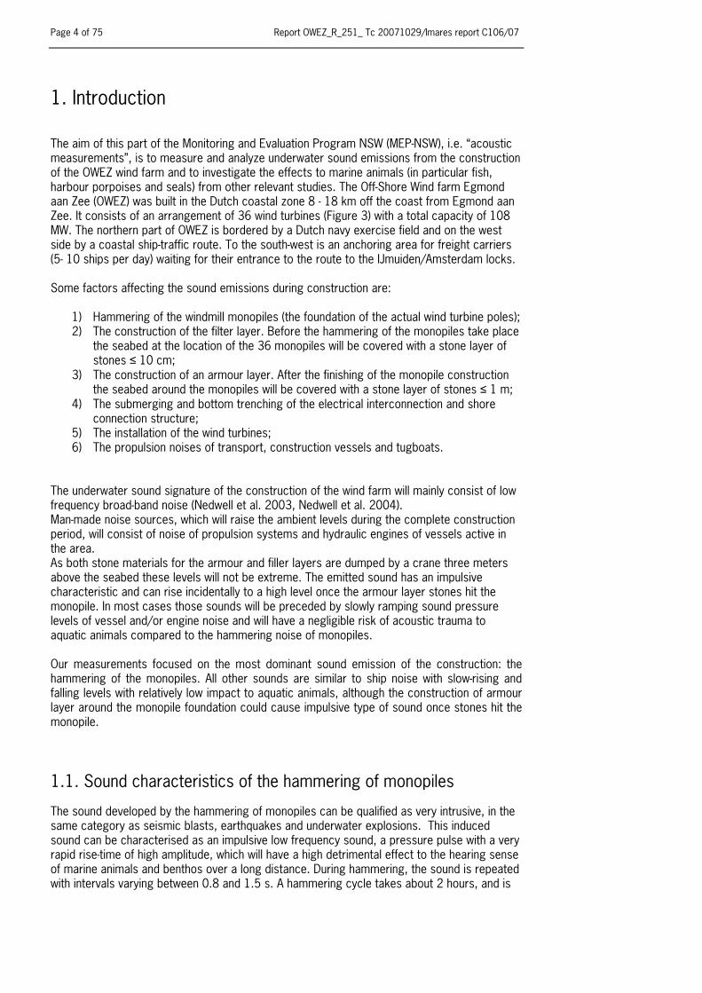
1.2.2. The determination of the Source Level (SL) of a sound source The Source Level (SL) of a specific emitted sound is defined at a nominal distance of 1 m, expressed in dB re 1 μPa at 1 m. However, in reality sounds are rarely measured at short distances, as sound characteristics in the near field of the source are irregular and complex to predict. The most reliable way to estimate the SL of larger sound sources is to take the appropriate distance and to measure the sound pressure in the far field, as illustrated in Figure 1 (Nedwell & Howell 2004). The region from the source to r0 is called the near field, the region beyond this range is called the far field.
Figure 1 Estimating the SL of a sound source by measuring the far field sound pressure levels (Nedwell & Howelll 2004). The threshold distance ( D ) of near-far field effects (line Fig 1) can be estimated as:
( ) λ/22
AcAFD =
×= ;
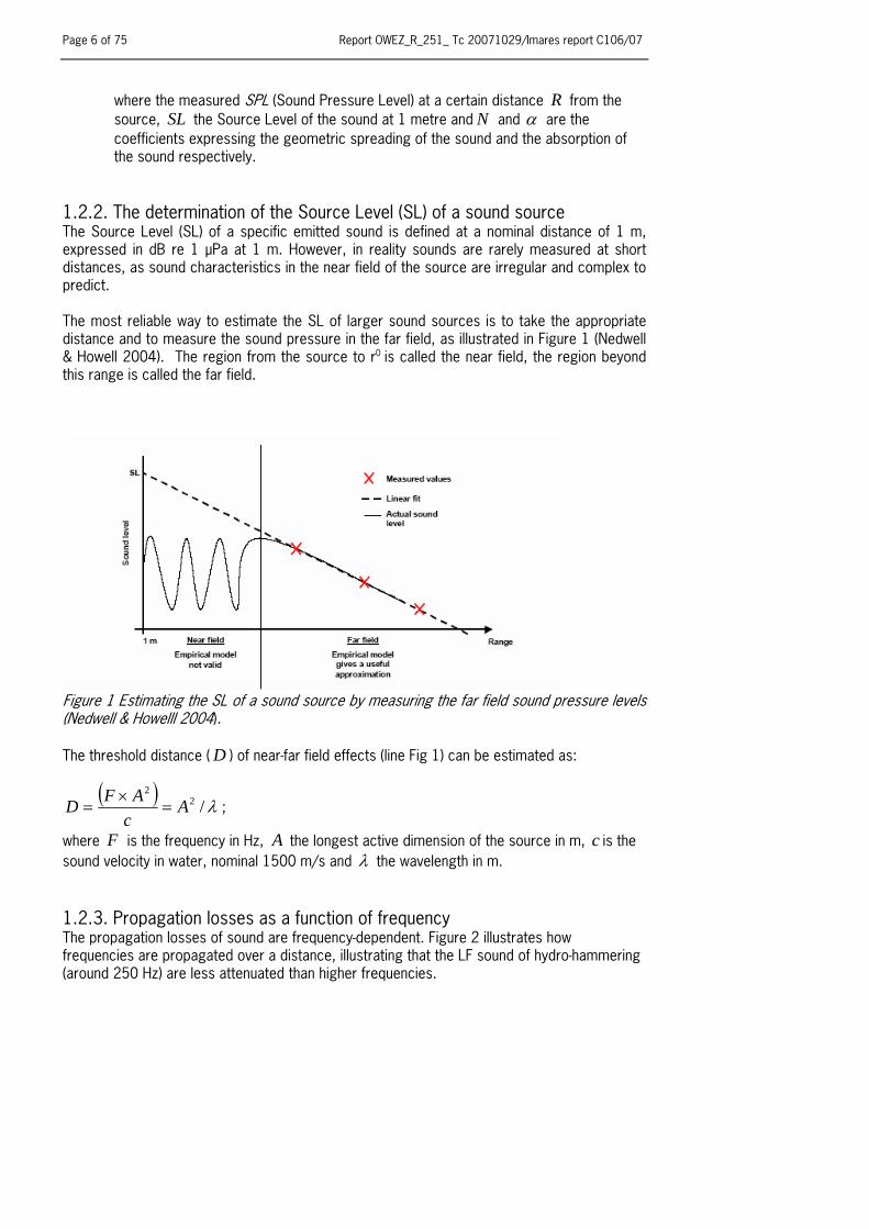
where F is the frequency in Hz, A the longest active dimension of the source in m, c is the sound velocity in water, nominal 1500 m/s and λ the wavelength in m. 1.2.3. Propagation losses as a function of frequency The propagation losses of sound are frequency-dependent. Figure 2 illustrates how frequencies are propagated over a distance, illustrating that the LF sound of hydro-hammering (around 250 Hz) are less attenuated than higher frequencies.
Report OWEZ_R_251_ Tc 20071029/Imares report C106/07 Page 7 of 75
Figure 2 Propagation losses as a function of frequency
To estimate the Source Levels of the monopile hammering it will be required to measure the sound pressure levels of the monopile hammering at a minimum of three different known distances of the sound source.
1.3. Sound characteristics of the hydro-hammer operation
The pile-driving sound signature is the result of a complex composition of variables. Basically the emitted sound spectrum will be related to the dimension of the sound source, the kinetic energy of the hammer on top of the monopile and the shape and size of the pile. These factors determine the level and frequency pattern of the emitted sound which will theoretically propagate omni-directionally as a result of the cylinder shape. However, due to the irregular bottom structure and variable water depth at the 36 hammering locations the emitted sound could propagate according a more complex model with variable transmission losses per case. The hammering of a single monopile takes approximately 1-2 hours depending on the seabed structure and the applied hammering energy. In the hammering cycle the next variables could play a role in the frequency spectra and levels of the emitted sound:
• The applied hammering energy. The applied energy of the hydro hammer will be the lowest at the start of the operation and is ramping up to the nominal energy after a number of blows. The energy curve will change per location as a result of the local seabed structure. The energy will also be coupled to the repetition rate of the hammering. The repetition rate could vary between 0.8 and 1.5 s. With the increasing penetration and energy the levels of the seismic seabed sound path could raise;
• The dimensions of the monopile. When the monopile is regarded as a sound projector the length and diameter will determine the wavelength and base frequency of the projected sound. The length of monopiles is a variable (section 2.1) and divided in four categories (Section 2.1) and the length part producing the sea-borne sound component reduces with the penetration into the seabed;
• The submerging of the hydro-hammer. The hammering will start with the hydro-hammer above the water surface. In this part of the cycle the monopile cylinder excites the monopile in the full water column. The submerging of the hydro-hammer as a result of the penetration could have an additional effect to the developed sound signature.
Page 8 of 75 Report OWEZ_R_251_ Tc 20071029/Imares report C106/07
Available publications of similar studies (Nedwell et al. 2003; Nedwell & Howell 2004; Anonymous 2001; Betke 2004) did not give insight on the relation of the applied hammering energy to the underwater developed sound signature. With the availability of kinetic data acquired during the hammering cycle, (such as the blow energy developed by the hydro hammer, the blow count and penetration depth of the monopile), it is possible to relate the recorded sound emissions to momentary kinetic data of the hydro hammer. This could give insight in the relation between the recorded sound signatures and the physical circumstances.
1.4. Hearing abilities of marine animals
1.4.1. Auditory thresholds of fish Fish use sound for a variety of functions including hunting, territorial behaviour, bonding, spatial orientation, predator detection, and escape. Most audiograms of marine fish species indicate that lowest sensitivity is in the 0.1– 2 kHz range. This narrow bandwidth of hearing sensitivity is hypothesised to be due to mechanical limitations of the sense organs (Astrup and Møhl, 1993, 1998; Motomatsu et al., 1998; Mann et al., 1997, 1998, 2001; 2005; Akamatsu et al., 1996, 2003). The auditory thresholds of some fish species are illustrated in Figure 4. Auditory threshold curves clearly differentiate between species with a swimbladder (cod) and those that without (dab). Not all fish species with swimbladder has a low hearing threshold. In a recent publication the role of the swimbladder serving as an auditory enhancement was doubted in relation to bony fish that are not provided with a Weberian Ossicles or Apparatus, a connection between the swimbladder and inner ear (Yan et al. 2000). Many have studied the effects of sound on the behaviour of marine fish (Moulton and Backus, 1955; Blaxter et al., 1981; Blaxter and Hoss, 1981; Fuiman et al., 1999; Enger et al., 1993; Knudsen et al., 1994; Luczkovich et al., 2000; Finneran et al., 2000; Lagardère et al., 1994 ; Løkkeborg and Soldal, 1993; Engås et al., 1996; Pearson et al., 1992; Skalski et al., 1992; Hawkins, 1986; Popper and Carlson, 1998; Wahlberg and Westerberg, 2005). Studies conducted in tanks could have underestimated the effects to fish species with a swimbladder. Animals exposed to a low water pressure (tanks or shallow water) could react differently to a specific sound under high water pressure condition (deeper water) the compressed gas-filled swimbladder could offset the acoustic sensing capabilities. Also the way the animals are caught and decompressed during the landing is an important issue to maintain a fully-functioning swimbladder/sensory system. Secondly behaviour of fish tested with pure tonals will differ to impulsive transient type of sounds with high rising edges. 1.4.2. Auditory thresholds of marine mammals As with fish, marine mammals use sound to navigate, forage and for bonding. Marine mammal species living in shallow coastal water habitats are harbour porpoises (Phocoena phocoena) and a pinniped harbour seals (Phoca vitulina). Cetaceans (toothed small whales and dolphins) produce and receive sound over a wide range of frequencies for use in communication, foraging, navigation and bonding (Tyack 1998). Cetaceans generate short transients, called clicks, for navigation and echo-location of prey at ranges of 10 to 100 meters (Au 1993). Most species also produce frequency modulated tonals, i.e. social calls also known as "whistles", to communicate (Tyack 1998). Pinnipeds (seals and sea lions) communicate in the frequency range from 50 Hz to 60 kHz (Richardson et al. 1995). Some auditory threshold spectra of marine mammals are illustrated in Figure 5a and b. The spectra of most pinnipeds (5a) show low thresholds in mid-frequency ranges of 0.2-50 kHz, while harbour porpoises are sensitive in high frequency ranges (5b). The detection of a sound through hearing sense of aquatic animals further depends on the presence and interference of noise in the specific frequency range of the sound. The interference effect is called masking and the frequency band in which this noise interferes is called the critical band (Richardson et al.. 1995). The perception of sound by aquatic animals is a ratio of the frequency, auditory threshold level and the masking ambient noise level. Our research will focus on this aspect i.e. the raised ambient levels of OWEZ wind farm related noise as well as a comparison of the outcome with other related studies.

Report OWEZ_R_251_ Tc 20071029/Imares report C106/07 Page 9 of 75
The very high impulsive sound pressures are developed on average 2000 times per monopile with a repetition rate of 1-1.5 s over a period varying between 1-2 hours (Nedwell et al. 2003, 2004) and can cause injuries to internal tissues, gas-containing organs, like swimbladder and lungs, gas embolisms in the bloodstream and eyes of animals in close range (Anonymous 2001). Specific data, however, on injuries to marine mammals, in particular their auditory systems, are very limited and levels that induce permanent threshold shift cannot made reliable (Ketten 2004). Model guidelines and international conventions have been developed, especially in relation to the operation of high level LF sonars used in naval exercises and the effects to marine mammals in particular cetaceans. These models were developed to predict gradients in safe and lethal distances, however, they are mainly based on data from terrestrial mammals held underwater (Turnpenny et al. 1994, Yelverton 1981) and partly on extrapolations of the human hearing sense (Yelverton, et al. 1973). Available data suggest that exposure to a narrowband sound for a protracted to short-term period of time, at a received level ranging typically from150-190 dB re 1 μPa and which is approximately 80-90 dB above the species-specific threshold, will induce temporary threshold shift (Ketten 2004). The hearing abilities of fish and marine mammals depend on a number of acoustic conditions and properties. Sound detection depends on the properties of the hearing sense of the target animal and the acoustic conditions. Ambient noise, the sound spectrum, and level of the specific sound source and the distance between the animal and the sound source and the sensitivity of the hearing sense of the animal are the main parameters. The detection of sound is related to ratio of the ambient noise level, the sound source level and the threshold level of the hearing sense of the animal at the specific frequency of the sound. These measures are called the critical ratio and the critical bandwidth. Ambient noise, unlike man-made sound sources, cannot be related to a particular direction or source, and has no dynamic behaviour in a specific volume. Therefore the SPL (Sound Pressure Level) will be the same everywhere and it is not necessary to specify the range at which it was measured at (cf. Source level). The level of the underwater noise and its ratio to the acoustic sensing capabilities of aquatic animals is an important measure for understanding the impact of hammering noise. Specifically, with larger coastal construction projects in permanent positions anthropogenic noises are coupled into seawater raising the traditional ambient levels incidentally or permanently. When these levels rise, either by environmental conditions or man-made noises, the detection of prey (foraging) or communication between aquatic animals could be jeopardised, as it becomes difficult to detect the target through all the background noise. The underwater acoustic background noise in a particular area will be an important factor for aquatic mammals to maintain their natural behaviour. It is possible that these animals could react by migrating to other areas when these levels affect their threshold detection levels.
1.5. Mitigation measures to deter marine mammals from the exposed area
As the frequency spectrum of the pile-driving spectrum measured in similar studies (Nedwell et al. 2003, 2004) mainly peaked in the lower part of the spectrum <1 kHz and the Sound Pressure Levels were in the range of 240 to 260 dB re 1μPa the sound will be propagated over long distances (>20 km). As the population of harbour porpoise in the Dutch coastal zone and numbers of strandings of harbour porpoise increased sharply (Camphuysen, 2005) there was concern on the effects of the hammering noise on harbour porpoises. With respect to these circumstances mitigation measures to deter harbour porpoises and seals from the exposed area is necessary and recommended for every monopile hammering case. The initiative to develop/organize a suitable technical measure was taken by the contractor/commissioner and on request of those parties an investigation was started, which lead to a suitable device (Section 2.10). The time period the deterrent sound was active was taken as long as possible (4 hrs) to allow animals with relatively lower swimming speed (seals) to leave the exposed area. A suitable marine mammal deterrent device would be a source emitting LF sound in the range of 0.25-10 kHz with a Source Level (SL) of around 190 dB rms re 1 μPa/1m. Based on knowledge derived from several sound studies with pingers and

Page 10 of 75 Report OWEZ_R_251_ Tc 20071029/Imares report C106/07
acoustic harassment devices (Kastelein et al. 2000 and 2005). Based on these behavioural observations it is believed that Harbour porpoises will migrate from the vicinity of the active deterrent and after successive hammering cases they will relate the sound to the hammering of the monopiles and start migrating from the exposed area as soon as the deterrent device is activated.
2. Methodology The measurements were conducted in the period the first hammering case started, on 17 April and on 28 July 2006 when the final hammering case took place, involving 6 hammering cases according the overview of Table 1. On the first case most of the measurements were carried out in the 2000-2400 m distance range. Three other distance ranges were incorporated to achieve some insight into the propagation of sound: this to be able to roughly estimate the SL in case of high impact on harbour porpoise (f.i. sudden high number of strandings after or during this first pile driving case). The two next pile-driving cases were used to determine the effects of the increasing energy cycle on the emitted sound pressure level in a one or two distance ranges. With these results the effects of the propagation of the sound at several distance ranges (monopile 10, 34 and 36) and the calculation of a Source Level could be determined with higher confidence. In those cases the propagation of the induced sound was investigated and measurements were carried out at several distances from the hammering location, varying between 500 and 4400 m. Measurement locations are shown in Figure 6. As the hammering of a single case was scheduled on a 24 hours cycle, the momentary tidal flow at the moment of a hammering case had to be taken as variable and varied per case. On the hammering of monopile 22 the tidal current was of such an order that a steady distance was maintained while floating up drift with the current. In this approach any irregular directivity patterns of the sound were not taken into account. On the hammering of monopile 36 the longest distance range was too close to the Gas Rig platform Q8B and this reference location (labelled 5) had to be adjusted to the north side perpendicular to the track of the shorter reference locations. A similar event, but more accidental occurred on the first case on the hammering of monopile 13 (location 1). Monopile 10 was hammered 10 m off the official position, the new position (X:593 452, Y:583 0943 UTM31 grid) was more in line with the other positions of the western row. As this updated UTM grid format caused a conflict in the conversion to the decimal position format the SL calculation analysis was not modified. Overview monopile measurements OWEZ wind park
Monopile (nr)
Date Distance ranges (m)
500-730
800-1065
1260-1510
2150-2434
2480-2660
3030-3150
3600-3760
4140-4320
13 17-04-2006 2 4 2 1 1 30-04-2006 5 3 22 04-05-2006 7 1 10 12-06-2006 1 3 3 3 2 3 36 27-07-2006 2 2 1 34 28-07-2006 3 2 3 1 2 3
Table 1 Overview of monopile measurement cases, distance ranges and numbers of data series.

Report OWEZ_R_251_ Tc 20071029/Imares report C106/07 Page 11 of 75
2.1. Monopile physics and construction data
Monopiles were constructed in 4 different length categories, adapted to the waterdepth at the actual defined position. The monopile overall length varied between 41 and 47 m. In all cases the overall diameter was 4.60 m with a wall thickness of 0.050 m. An overview of the relation of the dimensions of the monopiles with respect to the water depth conditions is shown in Table 2. Monopiles were hammered using the S-1200 hydro hammer (Figure 7c), which could develop a maximum of 1200 kJoule energy. The main construction tool was part of the rigging of the 8700 ton twin hulled heavy lift vessel ms “Svanen” (Figure 7a and b), on which monopiles were positioned and hammered. 2.1.1. Energy measurement The energy is measured inside the hydro-hammer by two time sensors, which measure the relative time of the falling speed of the hammer weight with which the energy is calculated (Figure 9 hydro-hammer principle). The result is decoupled from the applied energy changes and representative for the energy that is transferred to the pile, although as an effect of the losses in mechanical blow guiding adapters the true neat energy onto the pile will be 10-20% lower. Although the validity of the energy data is unknown and only used as reference trend per single pile-driving case, the unknown energy data error will relatively reduce in comparison of other cases.
Pile (nr)
Pile Toe Level
(m MSL)*
Seabed level (m)
Water level (NAP)
Water level
(MSL)*
Penetration (m)
13 -47.04 -18.8 28.2 1 -44.81 -19.7 0.65 0.55 25.1 22 -45.01 -19.1 0.44 0.34 25.9 10 -42.7 -17.6 -0.20 -0.30 25.1 36 -40.89 -18.4 -0.50 -0.60 22.5 34 -46.91 -18.0 0.40 0.30 28.9
*Seabed level MSL is the measured level before the application of filler layer onto the seabed Table 2 Overview of dimensions of monopiles in relation to water depth conditions at the locations
Pile (nr)
Cat. Pile Toe Level
(m MSL)*
Mass (tonnes)
Penetration (m)
Total time(s)
Net time (s)
Total applied
energy (kJ)
Total nr of blows
13 3 -47.04 242.8 28.2 02:05 00:49 1029832 2066 1 3 -44.81 232.7 25.1 02:16:06 00:50:21 1286592 2156 22 3 -45.01 232.7 25.9 02:02:47 00:41:16 1235051 2079 10 2 -42.7 212.6 25.1 05:10:35 01:05:42 1111005 3409 36 2 -40.89 202.5 22.5 01:09:38 00:48:37 1148657 2333 34 1 -46.91 216.5 28.9 01:28:04 01:09:02 1730251 3518
*Seabed level MSL is the measured level before the application of filler layer onto the seabed Table 3 Overview of main hammering data of the measurement cases and the applied kinetic energy Figure 8 shows the total applied energy and total number of blows of measured cases plotted against the pile-driving cases not measured. According to these data the hammering of monopile 34 was the heaviest case in terms of hammering energy. Monopile 10 and 13, although lowest in this selection, were still close to the average of cases, which were not measured.

Page 12 of 75 Report OWEZ_R_251_ Tc 20071029/Imares report C106/07
2.2. Measurement targets ranges and timing
2.2.1. Measurement targets Initially the first two hammering cases, two cases were nominal hammering energy was expected (22 and 10) and two cases were the highest energy range was foreseen (31, 3, 4 or 5). Of this original schedule the hammering cases of monopiles 13, 1, 22 and 10 were maintained, while the final hammering cases 36 and 34 replaced the planned high energy cases. The first two hammering cases (13 and 1) were executed in order to measure the impact from the start of the hammering in order to be able to produce acoustic data in case when a direct impact on marine animals was found. The original schedule could not be maintained due to a number of factors out of our control. At the start of the hammering cycle operations were jeopardized by bad weather. This meant the construction progress developed not as originally scheduled (a hammering cycle of 96 hours) but lower at the start and increasing in successive cases with a hammering cycle of 24 hours at the end of the hammering period. Under these circumstances the progress of the construction departed from the original IMARES planning, and a more flexible approach had to be accepted. Eventually 6 hammering cases were captured and analysed. However, the minimum proposed number of hammering cases did not affect the quality of the outcome. The range of selected hammering cases did include the case where the highest hammering energy was applied (monopile 34). Also the opportunity to weigh the acoustic received data with the actual applied energy outdated this aspect and increased the depth of the analysis, compared to available reports of similar studies. 2.2.2. Measuring distance ranges To avoid overload conditions as a technical consequence of the expected sound pressure levels and the lowest sensitivity setting of the acoustic sensing equipment, the measurements were conducted outside the boundaries of the construction area. During the measurements the ship's position (and so the hydrophone) was derived from the GPS position data from a GPS satellite receiver (Garmin 17 N type of GPS receiver), which was mounted on top of the ship’s bridge. The received GPS data (NMEA data string) were directly logged and stored on hard disc on an additional laptop computer and also used to monitor the ship’s position relative to the target and to navigate towards the target.
2.3. Weather conditions
The weather conditions during the 6 measurement cases were good to excellent. Wind force conditions did not exceed wind force 3 Bft.
2.4. Measurement platform
Measurements were conducted from a catamaran vessel type “WindCat” exploited by the company Bais Maritiem, Velsen-Zuid. The higher cruising speed (25 knots maximum) and the operation from the harbour of IJmuiden reduced the risk of not arriving at time off the activation of the acoustic target. This type of vessel was also exploited by the contractor for crew transits and operated in the area according the standard safety navigation regulations and were equipped for near- and offshore work with certificates from Dutch Shipping Inspection up to 60 nautical miles from the coastline worldwide. Detailed specifications of the vessel are given in Figure 10. During the measurements the ship switched-off all engines.
Report OWEZ_R_251_ Tc 20071029/Imares report C106/07 Page 13 of 75
2.5. Data collection and time reference
All internal clocks of recording equipment and computers were synchronized daily at the start of an experiment and referred to UTC (-1 hours of local Dutch time).
2.6. Description of the measurement equipment
2.6.1. Types of hydrophones and deployment Sound vibrations of the hydro hammer operation were converted to an analogue electric signal by use of a calibrated hydrophone (RESON TC 4033, SN 3504103) with a sensitivity of -201.8 dB re 1V/μPa and a flat response between 1 Hz- 80 kHz (+/-2.5 dB) (Figure 12, Response curve Reson TC4033 hydrophone). The hydrophone was suspended from the ship on its own 8 m long cable. Ambient noise, the acoustic emission of the AceAquatec deterrent device and the sound level of the Ducane Netmark 1000 reference source were measured by using a RESON TC 4032, SN 1704048 hydrophone. This more sensitive hydrophone contained a 10 dB internal pre-amplifier and was connected to a RESON EC 6073 input module, which facilitated as splitter for signal transfer and the powering of the hydrophone with a DC supply battery (PBQ 17 of 12.6 V/17Ah). Both hydrophones were suspended at a depth of 4 m in all cases and were not rigged with additional weight as the stretching forces would also add to strumming cable noises. The hydrophone was positioned leeward amidships on portside 1 m outside the side of the ship. 2.6.1. Conditioning of the hydrophone signal A battery powered amplifier (ETEC A1101) was used to amplify and filter the analogue hydrophone signal. The amplifier was equipped with a selectable gain of 0-50 dB and a high pass filter selectable in range of 1-100 kHz. The ambient measurements were conducted with a gain setting varying between 0-20 dB depending on the sea state conditions and the acoustic target and with a high-pass filter setting of 1 Hz to achieve the lowest possible influence on the LF part of the signals and secondly the conditions were excellent during the measurement, so compensation for hydrophone heave noise was not necessary. The frequency range of interest in which the hydrophone is sensitive is limited to a maximum of 200 kHz. As the gain characteristics of the A1101 amplifier were flat to 1MHz the amplifier would be sensitive to high frequency pick-up noise signals. To reduce all contribution outside the frequency range of the hydrophone the amplifier’s gain has was limited by a passive LC network connected to the output of the amplifier to filter the HF noise above 150 kHz with 12 dB/octave. The response curve of the A1101 (Figure 11) shows the effects of the low- and high-pass filter settings. At 10 Hz high-pass the response is – 3.35 dB at all three gain settings and at 100 kHz the response is + 2.2 dB. 2.6.2. A/D conversion of the analogue signal The conditioned analogue signal was connected via a coaxial input module (National Instruments, type BNC 2110) to a 18 bit data acquisition card (National Instruments, type PCI 6281M) on which the analogue signals were digitized. Aliasing normally occurs when the frequency spectrum of the signal contains components at or higher than half the sampling frequency (or rate). When these unrealistic components are not correctly filtered (or band limited) from the signal, they will show up as aliases or spurious lower frequency components that cannot be recognised from the valid sampled data. These errors in data are actually at a higher frequency, but when sampled, appear as a lower frequency, and thus contribute to false information. To reduce the effects of aliasing the analogue hydrophone signal was digitised with a sample rate of 512 kHz (data rate of 0.5 Msamples/s) with 16 bit resolution. The DAQ card was part of a PIV desktop computer. Data was acquired using an IMARES designed virtual instrument built with Labview 7.0 software (National Instruments). On this module the input limits were set to the estimated signal level from the A1101 amplifier to use the optimum of the 96 dB
Page 14 of 75 Report OWEZ_R_251_ Tc 20071029/Imares report C106/07
dynamic range of the DAQ card. Ambient noise measurements were mostly acquired with an input limit setting of +/- 0.5 V. Data files were stored on hard disc in a binary format and consisted of a data header, in which additional data, like the start time, sampling rate, gain input voltage range and filter settings were stored. Part of this header information (gain, distance and sampling rate) is used to scale the data in the analysis module.
2.7. Procedures of a single measurement
2.7.1. Positioning of the vessel towards a measurement location The approach of the ship to the measurement location was up-drift with wind and tidal conditions incorporated to position the vessel as close as possible towards the target location. The approach was monitored on a LCD monitor and logged on a computer using WINGPS software. The GPS logging facility was started in advance of the positioning. This logging was stopped once the hammering cycle was completed, all systems calibrated and on the return of the vessel towards IJmuiden harbour. Headers of all data files contained the activation time of the measurement, which was taken from the internal PC clock. This clock time was set to the GPS received time shortly before the measurement. When the ship approached the measurement location all engines were switched off and the hydrophone was suspended leeward to minimize the contribution of noise from breakwater to the measurements. An uninterruptible power supply (UPS) supplied the measuring equipment with AC 220 V, buffered by two PBQ rechargeable batteries. The highest noise immunity was obtained with ship’s ground reference disconnected from the AC supply. The ship’s VICTRON UPS power systems were switched off to minimise the effects of chopper noise on the measuring hardware. All other ship equipment was switched off. After the measurement cycle was fully prepared and propeller cavitations completely disappeared a measurement was started with the actual start time logged in the header of the data file. The data logging period was adapted to the record time and the number of distance ranges and varied between 50 and 195 seconds. The logging was interrupted when needed or when a hammering cycle was finished. After completion the hydrophone was taken on deck, the main engines started and the cycle repeated for a measurement on another location.
2.8. Accuracy of the measurements and uncertainties.
2.8.1. Hydrophone calibration and accuracy The Reson TC 4033 hydrophone was purchased in September 2004, the calibration certificate (Figure 12, Response curve of the Reson TC 4033 hydrophone) is dated 2004-09-27. The quality of the hydrophone is expressed in the response curves of the sensor in the horizontal and vertical plane. During measurements at sea the hydrophone was calibrated daily using the SPL/voltage relation of a pistonphone reference source (G.R.A.S., model 42AC), which generates a calibrated 250 Hz sinusoidal type of signal with a sound pressure level of 134 dB re 20 μPa (Figure 13, calibration certificate of the G.R.A.S. 42 AC pistonphone). The hydrophone reference pressure level was measured at the side gate of the hydrophone coupler using a class 1 type of sound level meter (B&K, type 2239, type C weighing filter) with the hydrophone coupled onto the pistonphone (Figure 14, hydrophone calibration set-up). With this instrument the opposed sound pressure level is known with an uncertainty of 0.2 dB (Figure 15a and b, Calibration certificates sound level meter B&K, type 2239). This hydrophone calibration procedure was executed for each cases, directly after the measurements to match the physical hydrophone conditions of the actual measurements (sea water temperature). The output signal of the hydrophone was acquired as separated calibration data file, which was used as scaling data in the analysis. During the calibration all the engines on board of the vessel were switched off. With this reference all system errors in the analogue/digital link were eliminated assuming a flat response curve of the hydrophone up to 80 kHz.

Report OWEZ_R_251_ Tc 20071029/Imares report C106/07 Page 15 of 75
The computer with the DAQ card was connected to a UPS (APC 1400) to cover the power supply interruptions when ship engines were switched off. Highest noise immunity was obtained when the ground reference of the amplifier/BNC chassis was referred to sweater by use of an additional ground terminal pole connected to the housing/support termination of the ETEC amplifier. 2.8.2. Reference measurements To increase the level of confidence, reference measurements were conducted as a part of the standard acoustic procedure with an acoustic reference source with known acoustic sound pressure level. In this case a 10 kHz Ducane Netmark 1000 pinger was used to check the acoustic scaling as reference for all measurement cases. The Ducane Netmark 1000 pinger was used in the research on the effects of acoustic deterrents to harbour porpoises (Kastelein, et al., 2000) and in other acoustic measurments as LF reference source (stable acoustic properties, omni-directional emission) to check the acoustic equipment as a standard procedure. The results showed that the fundamental frequency matched within 1 dB and the outcome of the harmonics up to 33 kHz within 2.5 dB to the outcome of the same pinger measured on 24-11-2005 in the outdoor basin ORCA of SEAMARCO, Wilhelminadorp. 2.8.3. Distance calculations and measurement locations The GPS received signals were tested in a stationary position over long time period > 48 hours at the IMARES laboratory, IJmuiden. GPS receiver plots were logged over a period of 4 days and the measured maximum deviation (Figure 16) of 11.7 m was within the specification of the manufacturer (specified max uncertainty 15 m). The uncertainty to the Source Level calculations will be inversely proportional with the distance and the highest at the shortest distance. When an uncertainty of 15 m is taken at 500 m distance as maximum distance error the error on the SPL result will be 0.25 dB. 2.8.4. Summary of system errors Taking al these possible errors (Table 4) in account the total error is rather low as the frequency band of interest is in the LF range, in which range (250 Hz) the TC 4033 hydrophone was calibrated per case and in the range where the response of the hydrophone is flat. System error
Equipment Error in dB hydrophone +/- 1 Pistonphone +/- 0.2 Distance 0.25 Table 4 System errors overview According this overview the total of these errors is 1.5 dB maximum. A higher effect on the results could however be the hydrophone depth in relation to the irregular directivity of the sound, the reverberations and irregular absorption coefficient by the shape of the seabed structure and the type of sediment. This contribution is complex and will be limited when the number of distance ranges are >4.
Page 16 of 75 Report OWEZ_R_251_ Tc 20071029/Imares report C106/07
2.9. Analysis and procedures
2.9.1. Analysis pocedures and selection of a time window The analysis of the hammering sound comprised two approaches to express acoustic properties:
• The calculation of the average sound pressure level over the complete pulse and the energy distribution in the frequency domain over this time period;
• The calculation of the sound pressure level of a shorter time fraction of the signal including the peak amplitude of the received signal and the energy distribution in the frequency domain over this shorter period.
Initially time samples of the blow signals were Fast Fourier transformed in two different time windows. A 0.2s time window (102564 samples) to express the energy over the complete pulse period and a second shorter time window of 0.06s (30769 samples) to express the peak value. However, the analysis showed that the 0.06 s time window would not always include the main peak amplitude at the longer distance ranges. Due to reverberant effects there were occasions when signals did peak in the aft part of the signal outside the selected 0.06 s time window (Figure 17). Secondly the 0.06 s time window was still too long in respect to the integration function of the FFT analysis, where peaks are time averaged and the actual peak amplitude would be underestimated. Therefore the dataset was reprocessed with two new time windows, a 0.1 s time window (51282) to express the energy over the complete pulse period and a 0.006 s time window (3077 samples) to include only the highest peak of the signal (Figure 18). The data records were first investigated in the time domain on amplitude variations (minimum/maximum peak to peak values) and quality throughout each recorded data file. Cases with high offset due to dynamic or instable hydrophone actions, with interference from battery operated power supplies were not negotiated and discarded from the analysis. Of all selected cases the processed sound pressure levels, peak to peak voltage of the highest amplitude and start time reference of the recorded signal were imported into a spreadsheet and sorted per distance range. Another analysis route was the processing of the distance of the hydrophone to the hammering location corresponding to the recorded sound files. These data blocks were retrieved from the GPS text files recorded during the measurements. These GPS files were imported in SAS statistic analysis software to sort the time period of interest and to calculate the distance to the monopile target location in steps of 1 second. The finalised datasets including the distance/SPL values, the hammering data of the hydro-hammer (blow energy, blow rate and timing) were than imported into a spreadsheet to synchronise the data to the GPS timing with the final blow as time cue. These final data were than imported in a DiaDem 9.1 spreadsheet (National Instruments) to execute the final mathematical functions (regression function) and to report results in a graph. 2.9.2. Analysis technique and spectrum analysis The analysis of the 16 bit binary data files was conducted on IMARES-designed software application tool using certificated standard virtual instruments built with Labview 7.0 software (National Instruments). The first step in the analysis was to load the calibration file of the specific time period, which was used to scale each data sample to the voltage/SPL relation of the pistonphone as measured with the B&K 2239 meter, this value scaled data samples to the calibrated dB value.

Report OWEZ_R_251_ Tc 20071029/Imares report C106/07 Page 17 of 75
The power FFT of hydrophone voltage samples, selected in a time series is computed in the analysis module using a virtual instrument (VI) “Power FFT” (National Instruments) and additional software VI to process spectrum units and to scale the result. In the analysis module the rms (route means square) sound pressure level ( rmsspl ) is calculated according the
formula:
⎟⎟⎠
⎞⎜⎜⎝
⎛= ∫
T
rms dtptp
Tspl
020
2)(1log10
where:
)(tp -single rms voltage sample proportional to sound pressure sample in Pa (Pascal).
οp -adapted minimum reference sound pressure level in water (1μPa).
The computed sound pressure level ( rmsspl ) represents the time-averaged sound pressure
amplitudes over the applied time windows (0.2, 0.1, 0.06 and 0.006s). There were two types of SPLs processed to express the levels of the received signals: SPL broad The computed SPLs were calculated from the rms value of the voltage amplitude of a given time window expressing the broad band result without specification of the frequency contribution. This value is particularly useful when the energy does not peak in a narrow frequency band but is spread over a wider range. SPL peak This value is the fast Fourier transformed SPL of the highest frequency of the spectrum. The energy could peak in more than one frequency, in that case those peaks were also listed. The frequency resolution, also expressed as bin width ( dF ) of the calculated FFT result depended on the selected time window, in case of a 0.1 s time window the frequency accuracy will be 10 Hz (sample rate/number of samples). Seismic waves were analysed with a time window of 0.04 s involving 20513 samples and a frequency resolution ( dF ) of 25 Hz. The “Hanning” window filter type was used to weigh the FFT result.
2.10. Mitigation measure to deter marine mammals from the exposed zone
Before a hammering cycle started, an autonomous deterrent device was used to deter harbour porpoise and seals from the exposed area and warn animals at longer radii (Figure 19). On request of the constructor a short inventory was conducted to propose an autonomous deterrent device strong enough to deter harbour porpoise from the TTS exposed radii. A Seal Scarer Device (SSD) manufactured by AceAquatec (GB) was advised to the constructer /commissioner as the most appropriate tool. Other competitive autonomous devices (deliverable within a time period of 4 weeks) were not available. The deterrent should have had an upramping onset to avoid damage to the hearing sense of marine mammals in close range. However given the timing of the request this mode could not be added to the instrument and it was assumed marine mammals, especially harbour porpoise, would not approach the area of monopile hammering position as ship-noise levels of the main ship and other involved vessels

Page 18 of 75 Report OWEZ_R_251_ Tc 20071029/Imares report C106/07
would be high. Secondly after the first event harbour porpoise would be recognised the scrammar sound and link it to the hammering noise. The acoustic properties were checked against the manufacturer's specifications on a separate mission organised by the constructer. It appeared the device operated according the specifications. The developed sound consists of a number of random selected "scrams", each 5 s long, with the maximum number/hour programmable and set to the maximum of 72. A series of scrams can be characterised as a "rattle" type of sound composed of a number of random ordered frequencies and time patterns. There are 19 primary frequencies ranging from 5 kHz to 20 kHz. Due to the type of sound the system produces odd harmonics. The system has a power band from 12 to 20 kHz at a Source Level of 194 dB re 1μPa @ 1m at 16 kHz. The ambient noise levels representative for the hammering condition at the given power band of the deterrent (Sea state 3-5) were measured at the wind farm location and were between 40-45 dB re 1μPa /√Hz (de Haan et al. 2006). According the hearing threshold level of harbour porpoise (Kastelein et al. 2002) at the SSD frequency range, the detection threshold level is masked by the ambient noise level. As a conclusion of this Critical Ratio (148 dB) the sound developed by the deterrent could be detectable at distances up to 10 km. The device was operated from the side of ms "Svanen" and submerged, directly after the anchoring phase of the ship was completed. This assured a minimum period of 4 hours before the hammering of a monopile would start. Assuming an average swimming speed of 0.8-0.9 m s-1, measured as average value against respiration over longer period of time in a tank (Otani et al. 2001). For seals the mean swim speed would be slightly lower. Mean swim speed from over 3000 dives from five grey seals tagged in Orkney and Shetland was 0.42±0.24 m s-1 (Sparling, 2003). After 4 hours harbour porpoise could have reached a distance of 12240 m under the referred condition and seals about 7200 m. The device was activated on submergence by a water switch and the produced emissions were loud enough to be detected on deck of the ship. Shortly before the start of the hammering the device was taken on deck. The device was redeployed in case the hammering was interrupted longer than 1 hour. On the six measurement cases the emission of the deterrent device was checked and measured at several distances. The receivals of the deterrent sound were confirmed to the operator on board ms "Svanen".

Report OWEZ_R_251_ Tc 20071029/Imares report C106/07 Page 19 of 75
3. Results
3.1. Time history of hammering sound
Figure 20 illustrates the sequence of a series of hammering blows recorded during the hammering of monopile 10 at a distance of 806 m from the hammering location. The amplitude changes such as those of the first and fifth blow occasionally occurred. On the logarithmic dB scale such a deviation would be 1.8 dB. Figure 21 illustrates the general time pattern of a single received hammering blow at short distance range (733 m) during the hammering of monopile 10. The signal shows the peak amplitude of the signal, the reverberations of the hammering noise as well as the seawater component of a seismic wave propagated through the seabed, which arrived just before the arrival of the signal received through the seawater path. This phenomenon was not related to the seawater path received blows as the wave was also present on the first blow of a series and was also reported in other similar studies (Nedwell et al.. 2003). As these seismic waves must have an impact to all seabed oriented animals including flatfish it was decided to analyse a few cases. These seismic signals were also investigated on the effects of increasing energy by taking a sample at the start and end of the hammering cycle (Section 3.2.4.). The overview of time signals during the hammering of monopile 10 (Figure 22) and 34 (Figure 23) at three different distance ranges showed a similar type of time pattern in case of monopile 10, but also changes in signal pattern (monopile 34), but with the amplitude as the only main variable.
3.2. Spectrum analysis of the monopile hammering cases
3.2.1. SPL data report of monopile 13 Data of the analysed hammering cases are summarized per case in Tables 5-a/f. Data
series
Anal Blows
Penetration Energy
AmplitudeMin/Max Distance SPL broad
(0.1s) SPL peak
(0.1s) SPL broad (0.006s)
SPL peak (0.006s)
(nr) (nr) (m) (kJ) V p/p (m) [dB re 1 μPa (rms)] (StDev) 1 7 (45) 15.5 65 0.15/0.28 1487 174 (1.3) 170 (1.5) 179 (1.6) 179 (1.6)2 11 (167) 20.25 126 0.32/0.53 1514 178 (1.3) 172 (2.2) 184 (1.5) 184 (1.9)3 7 (50) 22.25 480 0.05/0.07 3652 160 (0.6) 152 (0.6) 164 (1.0) 163 (1.4)4 11 (169) 23.5 578 0.12/0.20 2382 170 (0.8) 161 (1.7) 174 (1.1) 174 (0.9)5 8 (61) 24 577 0.11/0.19 2367 169 (1.3) 161 (2.2) 173 (1.7) 170 (4.0)6 11 (89) 24.5 578 0.10/0.15 2350 169 (0.7) 161 (1.3) 172 (1.7) 172 (2.4)7 14 (163) 25 576 0.11/0.21 2294 170 (1.0) 162 (1.4) 175 (1.8) 175 (3.1)8 6 (13) 27 674 0.03/0.05 3145 157 (0.9) 147 (1.6) 161 (0.7) 158 (2.1)9 10 (87) 27.25 707 0.05/0.07 3034 159 (0.6) 151 (0.9) 163 (1.5) 161 (2.7)
StDev max 1.3 2.2 1.8 4.0 Table 5a Overview of the measured SPLs (with standard deviation per data series) per data series of the hammering of monopile 13, the number of analysed blows (total number of measured blows) and the measured minimum and maximum voltage (peak to peak) of the highest amplitude of all measured signals against the penetration depth and the applied energy.
Page 20 of 75 Report OWEZ_R_251_ Tc 20071029/Imares report C106/07
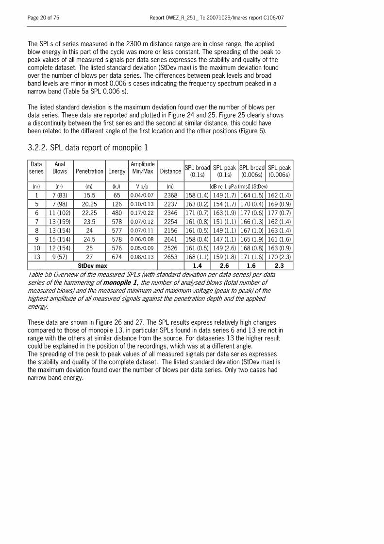
The SPLs of series measured in the 2300 m distance range are in close range, the applied blow energy in this part of the cycle was more or less constant. The spreading of the peak to peak values of all measured signals per data series expresses the stability and quality of the complete dataset. The listed standard deviation (StDev max) is the maximum deviation found over the number of blows per data series. The differences between peak levels and broad band levels are minor in most 0.006 s cases indicating the frequency spectrum peaked in a narrow band (Table 5a SPL 0.006 s). The listed standard deviation is the maximum deviation found over the number of blows per data series. These data are reported and plotted in Figure 24 and 25. Figure 25 clearly shows a discontinuity between the first series and the second at similar distance, this could have been related to the different angle of the first location and the other positions (Figure 6). 3.2.2. SPL data report of monopile 1 Data
series
Anal Blows
Penetration Energy
Amplitude Min/Max Distance SPL broad
(0.1s) SPL peak
(0.1s) SPL broad (0.006s)
SPL peak (0.006s)
(nr) (nr) (m) (kJ) V p/p (m) [dB re 1 μPa (rms)] (StDev) 1 7 (83) 15.5 65 0.04/0.07 2368 158 (1.4) 149 (1.7) 164 (1.5) 162 (1.4) 5 7 (98) 20.25 126 0.10/0.13 2237 163 (0.2) 154 (1.7) 170 (0.4) 169 (0.9) 6 11 (102) 22.25 480 0.17/0.22 2346 171 (0.7) 163 (1.9) 177 (0.6) 177 (0.7) 7 13 (159) 23.5 578 0.07/0.12 2254 161 (0.8) 151 (1.1) 166 (1.3) 162 (1.4) 8 13 (154) 24 577 0.07/0.11 2156 161 (0.5) 149 (1.1) 167 (1.0) 163 (1.4) 9 15 (154) 24.5 578 0.06/0.08 2641 158 (0.4) 147 (1.1) 165 (1.9) 161 (1.6) 10 12 (154) 25 576 0.05/0.09 2526 161 (0.5) 149 (2.6) 168 (0.8) 163 (0.9) 13 9 (57) 27 674 0.08/0.13 2653 168 (1.1) 159 (1.8) 171 (1.6) 170 (2.3)
StDev max 1.4 2.6 1.6 2.3 Table 5b Overview of the measured SPLs (with standard deviation per data series) per data series of the hammering of monopile 1, the number of analysed blows (total number of measured blows) and the measured minimum and maximum voltage (peak to peak) of the highest amplitude of all measured signals against the penetration depth and the applied energy. These data are shown in Figure 26 and 27. The SPL results express relatively high changes compared to those of monopile 13, in particular SPLs found in data series 6 and 13 are not in range with the others at similar distance from the source. For dataseries 13 the higher result could be explained in the position of the recordings, which was at a different angle. The spreading of the peak to peak values of all measured signals per data series expresses the stability and quality of the complete dataset. The listed standard deviation (StDev max) is the maximum deviation found over the number of blows per data series. Only two cases had narrow band energy.

Report OWEZ_R_251_ Tc 20071029/Imares report C106/07 Page 21 of 75
3.2.3. SPL data report of monopile 10 Data
series
Anal Blows
Penetration Energy
AmplitudeMin/Max Distance SPL broad
(0.1s) SPL peak
(0.1s) SPL broad (0.006s)
SPL peak (0.006s)
(nr) (nr) (m) (kJ) V p/p (m) [dB re 1 μPa (rms)] (StDev) 2 6 (26) 5 77 0.05/0.08 4144 164 (1.9) 163 (1.9) 169 (1.9) 167 (2.8)3 8 (40) 5.5 79 0.06/0.07 4210 163 (1.1) 162 (1.0) 168 (1.1) 167 (1.3)4 7 (48) 8.5 266 0.05/0.07 4311 162 (1.4) 159 (2.0) 167 (1.4) 165 (3.4)5 6 (68) 9 15 0.05/0.10 2483 164 (1.7) 156 (0.9) 168 (1.9) 165 (2.7)6 12 (202) 9.25 6 0.04/0.06 2627 161 (0.7) 153 (0.7) 164 (0.8) 165 (1.2)7 5 (121) 9.5 7 0.09/0.10 1448 166 (1.3) 161 (2.4) 172 (1.0) 172 (0.9)8 10 (120) 10.75 161 0.37/0.58 806 178 (1.0) 170 (1.4) 185 (1.0) 185 (1.3)9 6 (70) 11.75 219 0.43/0.58 882 178 (0.3) 172 (0.4) 185 (1.5) 184 (2.1)10 7 (76) 12 243 0.39/0.44 956 177 (0.3) 170 (0.8) 184 (0.2) 184 (0.2)11 5 (65) 13.75 463 0.09/0.11 1395 165 (0.9) 158 (1.0) 171 (0.6) 171 (1.0)12 7 (91) 16 525 0.13/0.18 2541 169 (1.1) 161 (1.4) 175 (0.9) 175 (1.0)13 6 (52) 17.75 549 0.09/0.11 3652 166 (0.4) 158 (0.8) 172 (0.5) 172 (0.6)14 7 (78) 18.25 547 0.09/0.10 3694 165 (0.2) 159 (1.6) 171 (0.3) 172 (0.3)18 6 (27) 24.75 777 0.28/0.34 1444 175 (0.3) 170 (0.4) 181 (0.3) 181 (0.4)19 3 (3) 25.25 799 0.45/0.51 734 178 (0.3) 169 (0.9) 184 (0.4) 184 (0.4)
StDev max 1.9 2.4 1.9 3.4 Table 5c Overview of the measured SPLs (with standard deviation per data series) per data series of the hammering of monopile 10, the number of analysed blows (total number of measured blows) and the measured minimum and maximum voltage (peak to peak) of the highest peak of all measured signals against the penetration depth and the applied energy. These data are shown in the energy/penetration reference graph (Figure 28). Figure 28 shows that the SPLs measured at 806 m at the start of the hammering cycle (161 kJoule) were in the same range of those measured at the end of the cycle at 734 m with highest blow energy (799 kJoule). The complete data series (n blows) were plotted in the distance reference graphs to achieve full resolution of the calculation of the regression functions (Figures 28 and 29. The listed standard deviation is the maximum deviation found over the number of blows per data series.

Page 22 of 75 Report OWEZ_R_251_ Tc 20071029/Imares report C106/07
3.2.4. SPL data report of monopile 22 Data
series
Anal Blows
Penetration Energy Amplitude
Min/Max Distance SPL broad (0.1s)
SPL peak (0.1s)
SPL broad (0.006s)
SPL peak (0.006s)
(nr) (nr) (m) (kJ) V p/p (m) [dB re 1 μPa (rms)] (StDev) 1 12 (59) 28 125.1 0.20/0.32 2348 175 (1.0) 171 (1.2) 181 (1.4) 181 (1.6) 2 16 (245) 31.25 275.6 0.14/0.21 2565 172 (0.6) 166 (1.1) 177 (0.6) 177 (0.7) 3 13 (191) 39.25 721.5 0.22/0.30 2352 174 (0.5) 167 (2.2) 180 (0.5) 179 (0.6) 4 11 (143) 40.75 818.4 0.12/0.24 2360 171 (1.5) 164 (2.2) 175 (2.1) 174 (2.4) 5 7 (62) 41.75 757 0.14/0.23 2347 172 (1.3) 165 (1.7) 177 (1.2) 177 (1.2) 6 9 (105) 42.25 805.3 0.10/0.15 2358 169 (0.9) 161 (0.9) 173 (1.3) 172 (2.2) 7 12 (134) 43 826 0.11/0.15 2383 169 (0.4) 161 (0.8) 173 (0.4) 173 (1.0) 8 8 (80) 44.25 822.9 0.07/0.04 2426 168 (0.7) 161 (1.2) 172 (0.7) 171 (1.4)
StDev max 1.5 2.2 2.1 2.4 Table 5d Overview of the measured SPLs (with standard deviation per data series) per data series of the hammering of monopile 22, the number of analysed blows (total number of measured blows) and the measured minimum and maximum voltage (peak to peak) of the highest peak of all measured signals against the penetration depth and the applied energy. These data are shown in Figures 30 and 31. SPLs decreased in the order of execution of the measurements indicating a directivity influence as measurements were taken at different angles (Figure 6 measurements locations). Location of data series 4, 6, 7, and 8 were in close range and so were the measured SPLs in those cases. Location of data series 2 had the highest angle deviation, which can be seen in the SPL value, also this case was measured in deeper water (Figure 6). 3.2.5. SPL data report of monopile 36 Data
series
Anal Blows
Penetration Energy
Amplitude Min/Max Distance SPL broad
(0.1s) SPL peak
(0.1s) SPL broad (0.006s)
SPL peak (0.006s)
(nr) (nr) (m) (kJ) V p/p (m) [dB re 1 μPa (rms)] (StDev) 1 15 (159) 23.5 86 0.39/0.91 678 180 (1.4) 176 (1.4) 187 (1.9) 187 (2.1) 2 6 (17) 27 273 0.90/1.06 508 183 (0.4) 174 (1.2) 191 (0.8) 191 (1.2) 3 7 (108) 28.5 465 0.49/0.61 1065 179 (0.3) 171 (0.4) 186 (0.8) 186 (1.1) 4 7 (64) 31.25 459 0.49/0.71 908 178 (0.1) 171 (0.4) 185 (0.7) 180 (2.1) 5 10 (148) 36.75 641 0.16/0.20 2325 169 (0.7) 162 (1.4) 176 (0.4) 175 (1.2)
StDev max 1.5 2.2 2.1 2.4 Table 5e Overview of the measured SPLs (with standard deviation per data series) per data series of the hammering of monopile 36, the number of analysed blows (total number of measured blows) and the measured minimum and maximum voltage (peak to peak) of the highest amplitude of all measured signals against the penetration depth and the applied energy. These data are shown in Figures 32 and 33. Figure 32 shows that the SPLs were mainly proportional to the distance range. Figure 33 shows that the calculated regression function matches both time window cases as well as the results of data series were more in line than in other cases, although the min/max amplitudes of dataseries 1 had a wider range (and that the different angle of the position of dataseries 5 had no effect on the result.
Report OWEZ_R_251_ Tc 20071029/Imares report C106/07 Page 23 of 75
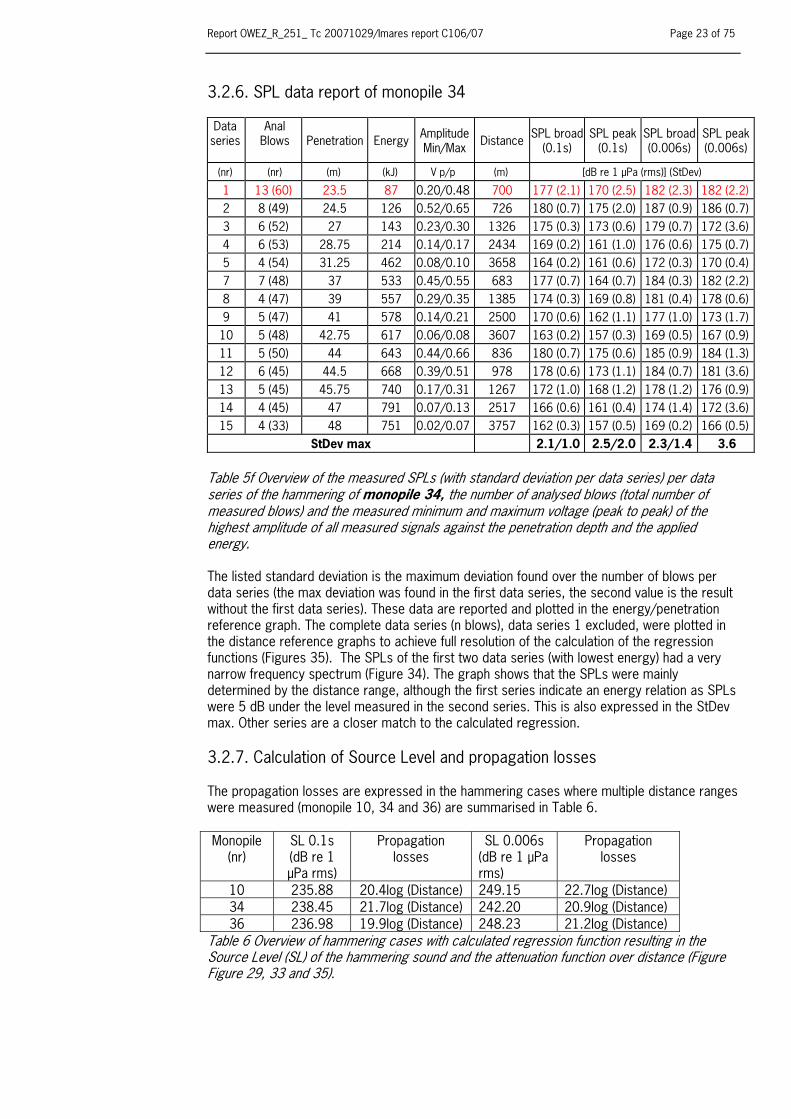
3.2.6. SPL data report of monopile 34 Data
series
Anal Blows
Penetration Energy Amplitude
Min/Max Distance SPL broad (0.1s)
SPL peak (0.1s)
SPL broad (0.006s)
SPL peak (0.006s)
(nr) (nr) (m) (kJ) V p/p (m) [dB re 1 μPa (rms)] (StDev) 1 13 (60) 23.5 87 0.20/0.48 700 177 (2.1) 170 (2.5) 182 (2.3) 182 (2.2)2 8 (49) 24.5 126 0.52/0.65 726 180 (0.7) 175 (2.0) 187 (0.9) 186 (0.7)3 6 (52) 27 143 0.23/0.30 1326 175 (0.3) 173 (0.6) 179 (0.7) 172 (3.6)4 6 (53) 28.75 214 0.14/0.17 2434 169 (0.2) 161 (1.0) 176 (0.6) 175 (0.7)5 4 (54) 31.25 462 0.08/0.10 3658 164 (0.2) 161 (0.6) 172 (0.3) 170 (0.4)7 7 (48) 37 533 0.45/0.55 683 177 (0.7) 164 (0.7) 184 (0.3) 182 (2.2)8 4 (47) 39 557 0.29/0.35 1385 174 (0.3) 169 (0.8) 181 (0.4) 178 (0.6)9 5 (47) 41 578 0.14/0.21 2500 170 (0.6) 162 (1.1) 177 (1.0) 173 (1.7)10 5 (48) 42.75 617 0.06/0.08 3607 163 (0.2) 157 (0.3) 169 (0.5) 167 (0.9)11 5 (50) 44 643 0.44/0.66 836 180 (0.7) 175 (0.6) 185 (0.9) 184 (1.3)12 6 (45) 44.5 668 0.39/0.51 978 178 (0.6) 173 (1.1) 184 (0.7) 181 (3.6)13 5 (45) 45.75 740 0.17/0.31 1267 172 (1.0) 168 (1.2) 178 (1.2) 176 (0.9)14 4 (45) 47 791 0.07/0.13 2517 166 (0.6) 161 (0.4) 174 (1.4) 172 (3.6)15 4 (33) 48 751 0.02/0.07 3757 162 (0.3) 157 (0.5) 169 (0.2) 166 (0.5)
StDev max 2.1/1.0 2.5/2.0 2.3/1.4 3.6 Table 5f Overview of the measured SPLs (with standard deviation per data series) per data series of the hammering of monopile 34, the number of analysed blows (total number of measured blows) and the measured minimum and maximum voltage (peak to peak) of the highest amplitude of all measured signals against the penetration depth and the applied energy. The listed standard deviation is the maximum deviation found over the number of blows per data series (the max deviation was found in the first data series, the second value is the result without the first data series). These data are reported and plotted in the energy/penetration reference graph. The complete data series (n blows), data series 1 excluded, were plotted in the distance reference graphs to achieve full resolution of the calculation of the regression functions (Figures 35). The SPLs of the first two data series (with lowest energy) had a very narrow frequency spectrum (Figure 34). The graph shows that the SPLs were mainly determined by the distance range, although the first series indicate an energy relation as SPLs were 5 dB under the level measured in the second series. This is also expressed in the StDev max. Other series are a closer match to the calculated regression. 3.2.7. Calculation of Source Level and propagation losses The propagation losses are expressed in the hammering cases where multiple distance ranges were measured (monopile 10, 34 and 36) are summarised in Table 6. Monopile
(nr) SL 0.1s (dB re 1 μPa rms)
Propagation losses
SL 0.006s (dB re 1 μPa rms)
Propagation losses
10 235.88 20.4log (Distance) 249.15 22.7log (Distance) 34 238.45 21.7log (Distance) 242.20 20.9log (Distance) 36 236.98 19.9log (Distance) 248.23 21.2log (Distance)
Table 6 Overview of hammering cases with calculated regression function resulting in the Source Level (SL) of the hammering sound and the attenuation function over distance (Figure Figure 29, 33 and 35).

Page 24 of 75 Report OWEZ_R_251_ Tc 20071029/Imares report C106/07
The calculated Source Level for monopile 34 were 3 to 5 dB lower than the other two cases, which were driven with lower energy ratings. The origin for this lower estimate is expressed in the higher SPLs of the monopile 34 data at medium (>1300 m) and higher distances (>2400 m, which implies a lower regression. The higher values at medium ranges must have been related to stronger reverbs. Therefore the SL result of monopile 34 could be an underestimate of the actual Source Level value. 3.2.8. Frequency aspects of hammering Two examples of spectrum results measured in the data series of monopile 10 are illustrated in Figure 36. A sample measured at a distance of a distance of 734 m (a) data series 15, case 2 and a sample of data series 10 case 2 at 1384 m. Sample rate 512 kHz, time window 0.1 s, 51282 samples, dF 10 Hz. The first case expressed a peak level 171.6 dB re 1μPa at 165 Hz, with also lower contribution at 70 Hz (-11 dB) and the second case energy in a wider band with peak level of 161 dB re 1μPa at 180 and 330 Hz, with also lower contribution at 80 Hz (-11 dB). Both cases express a low-frequency cut-off up to 150 Hz. 3.2.9. Seismic waves As shown in the basic overview of received hydro-hammer blow a diffracted component of a seismic seabed-borne signal arrived just in front of the seawater-borne sound of the hammering blow (Figure 21). This phenomenon was not related to the seawater-borne path received signals as the wave was also detected on the very first blow of a series and was also reported in other similar studies (Newell et al. 2003). As these seismic waves will have an impact to all seabed oriented animals the relation between SPL and hammering energy were investigated on the effects of increasing energy on two hammering cases (monopile 10 and 34) at a short distance range (approx. 800 m) by taking a sample at the start and end of the hammering cycle (Figure 37 and 38). It appeared the effects of the increased energy could be clearly demonstrated in the analysed seismic levels. At the end of the hammering cycle of monopile 34 the broad band level raised with 12 dB to 170 dB, the level of seismic wave of monopile 10 raised with 8 dB to 168 dB (Table 7). The spectrum was narrow and peaked at 125 (low energy case) and 130-150 Hz (high energy case).
Seismic wave monopile 34 data series 2 and 11 Data series
Distance (m)
Time in file
Energy (kJ)
Ampl (Vp/p)
SPL broad
SPL peak
Freq peak (Hz)
2 726 3.117 126 0.019 154.91 153.15 125 11 811 47.559 668 0.064 167.44 164.81 144
Table 8 Overview of increased SPLs of diffracted sea-borne seismic waves on two different hammering cases at similar distance ranges as a function of increased energy.
Seismic wave monopile 10 data series 8 and 19 Data
Series (nr)
Distance (m)
Time in File (s)
Energy (kJ)
Ampl (Vp/p)
SPL broad [dB re 1 μPa
(rms)]
SPL peak [dB re 1 μPa
(rms)] Freq peak
(Hz)
8 882 126.57 219 0.023 157.23 157.61 125
19 734 2.815 799 0.060 165.49 163.47 125/150

Report OWEZ_R_251_ Tc 20071029/Imares report C106/07 Page 25 of 75
4. Conclusion
4.1. Selected hammering cases, energy relation and measured Sound Pressure Levels
In terms of applied hammering energy the six measured hammering cases were fully representative for the other 30 construction cases with even one the measured cases (monopile 34) as the case with highest applied energy. The results clearly demonstrate that the applied hammering energy hardly had an effect on the exposures measured during the construction of monopile 10, 22, and 36 and only in the very first blow series of monopile 34. Given the consistency of the results and the close match of the estimated regression of all three hammering cases (monopile 10, 34 and 36), the difference in the timing of the measurements did not play a role in the outcome. Sound pressure levels measured at constant distance (monopole 13 and 22) measured at low and high hammering energy rates at the start and end of the hammering cycle were a close match. The effect of the seabed structure and as a result the possible irregular directivity pattern of the emitted sound and the fact that in some cases the measurements were not conducted in a straight track were observed in results and locations of monopile 22 and in the first result and location of monopile 13. The first case of monopile 13 was due to a communication error in positioning the vessel. The decreasing sound pressure levels in the order of execution of monopile 22 (Figure 31) indicate a directivity influence as measurements were taken at different angles (Figure 6). The background for the different angles in the positioning towards the monopile 22 was related to the relatively high tidal current at the moment of the construction. Dataseries 6, 7 and 8 of monopile 22 were taken in positions in close range and so were the measured SPLs. The different angle of position of data series 5 towards monopole 36 was related to the close presence of the Q8B gas rig at that given distance and the fact that the hammering started unexpectedly earlier. Results of data series 5, however, matched the other data series expressed by the calculated regression (Figure 33). The difference of the pile length and the progressive reduction of the height as a result of the hammering could not be recognised in the frequency spectra of the hammering cases. The estimated broadband Source Levels measured over the highest amplitude of the received signal were in the range of 242-248 dB re 1 μPa (rms), which can be categorised as very high impulsive sound exposures, causing injuries to aquatic animals at close range and acoustic trauma to those at longer ranges. The SPLs measured in the present study compared to those reported in other projects are in the same range. On the construction of the pile foundation of the Oakland Bay Bridge, San Francisco, U.S (Anonymous 2001), where piles of 2.40 m diameter were driven with a hydro-hammer of 1 MJoule, a Source Level estimate of 240 dB re 1μPa was developed according a transmission loss of 20 log(Distance). The SPL results reported of wind farms similar to the physical dimensions of the OWEZ facility, like the North Hoyle facility 5 miles off the north Wales coast with monopiles of 50 m long and 4 m diameter and the Scroby Sands wind farm, 2 miles off the Great Yarmouth coast with monopiles of 40-50 m long and 4.20 m diameter, are a very close match (Nedwell et al. 2003) to those found in the present study. On the North Hoyle project monopiles were driven by a Menck MHU500T with 450 kNm at 35 blows per minute with estimated peak to peak Source Levels of 262 dB re 1 μPa, measured on a water depth of 10 m. Also these results follow a similar regression of 22 Log (Distance). The present broadband Source Levels are probably underestimated as expressed by the low-frequency cut-off < 300 Hz, illustrated in Figure 36a and b. At an average waterdepth of 16 m lower frequencies cannot propagate and are “trapped” in the sound channel. This phenomenon was also found in other shallow water pile-driving cases (Madsen et al. 2006). The results reported from the Scroby Sands construction showed similar sound levels, although the number of data at several distances were low resulting in a very high uncertain
Page 26 of 75 Report OWEZ_R_251_ Tc 20071029/Imares report C106/07
regression of 36 Log Distance. Also varying water depth of around 10 m, variations of 5 m depending on high tidal effects occur, could have influenced this strong regression. The results reported from the Mecklenburg facility followed a 16 log Distance (Betke et al 2003), the North Hoyle location, with a water depth of 7-11 m, a 22 log (Distance) regression (Nedwell et al. 2003), the Horns Reef a 18 log (Distance) regression (Anonymus 2002). Summarised the present regressions estimates show that the transmission losses of the present study is a realistic result, which could also be valid for estimating of the Source Level from the single point result, measured in the same area of underwater explosions recorded during the baseline period of this project (de Haan 2006). Seismic waves The effects of the seabed-borne seismic wave path on all seabed oriented animals could be significant over a large range and so far little evidence could be found in literature. The diffracted sea-borne component of seismic wave received just in front of the sea-borne sound signal was proportional to the hammering energy and penetration depth. Results from monopile 10 and 34 showed the broad band level raised with respectively 8 dB to 168 dB re 1 μPa and with 12 dB to 170 dB re 1 μPa. The frequency spectrum peaked in a narrow band at 125 Hz (low energy case) and somewhat wider at 130-150 Hz (high energy case). The occurrence and the amount of sea-borne measured energy share is an indication of a much larger seabed-borne component proportional to hammering energy and penetration depth.
5. Discussion
5.1. Limitations of the measurements
Emissions of single point spherical sound sources are normally measured with the hydrophone depth equal to that of the depth of the transducer. Multiple paths are produced of which the effects to the received hydrophone signal depend a complex model of reverberations and absorptions of the sound with factors, like bottom structure, water depth and salinity as main variables. Due to the fact that the monopole length fitted the water depth it was assumed that sound exposures developed during monopole hammering would have exited the complete water column rather than a single point exposure. The results were measured at a single fixed water depth of 4 m, so sound paths in other sound channels remained unknown. On a project of similar dimensions, the North Hoyle wind farm, the sound exposures of monopile hammering were measured at two different water depths (5 and 10 m). The estimated Source Levels measured under these conditions only deviated 2 dB re 1 μPa (Nedwell et al. 2003). It is therefore believed the uncertainty of the results in the present study is limited to a similar rating. The approach of measurements at more than one water depth would have increased the time needed per single distance range and would have limited the number of distance ranges. In the present study measurements at single distance could be repeated in the hammering cycle and it showed that the influence of the penetration depth and applied hammering energy on the measured SPLs were low.
5.2. Effects of the hammering sound to marine animals
5.2.1. Fish As no experiments were conducted with fish during the pile driving this part of the study refers to existing literature of similar projects. Injuries in fish due to sound exposure have been reported in several studies.
Report OWEZ_R_251_ Tc 20071029/Imares report C106/07 Page 27 of 75
Caged pacific salmon (Onchorhynchus spp.) exposed to a sound exposure equivalent to SPLs of the present study during the hammering of monopiles for the Oakland Bridge foundations near San Francisco, U.S. showed that the fish opposed to the sound within 50 m died immediately and fish at 1000 m from the pile driving location were seriously injured and would have died within a short time period after the exposure. Tests on caged fish revealed greater effects when using a larger hydro hammer (1700 KJoule) rather than a 500 KJoule device. Enger (1981) reported that cod (Gadus morhua) exposed to frequencies between 50-400 Hz at 180 dB re 1 μPa for a period of 1-5 hours destructed ciliary bundles in the sensory epithelia. Denton and Gray (1993) observed the destruction of hair cells in the lateral line organ in clupeids by exposures to a sound pressure level of 153-170 dB re 1μPa. However, according the review of Hastings and Popper (2005) no clear correlation between the level of the sound exposure and the degree of damage could be determined. 5.2.2. Marine mammals At present the increased concern in public and in international marine mammal societies on the effects of intensive sounds and the coincidence of these sounds on marine mammals (mass strandings of whales) demand for internationally adapted guidelines on the conditions of operations of these activities and definition of safe exposure threshold levels. To predict safe zones for cetaceans in relation to high level sound exposures, for example the influences and effects of seismic equipment (airgun arrays), LF Navy sonars to cetaceans, internationally adapted models and guidelines were developed to produce gradients in safe and lethal distances for different categories of cetaceans (Verboom, 1999). These models are mainly based on data from terrestrial mammals held underwater (Yelverton et al.. 1973, Yelverton 1981) and assumptions and extrapolations of the human hearing sense. There are three agreed gradients of the impact of exposed sound levels to the hearing sense:
a) The PTS (Permanent Threshold Shift) gradient of direct hearing damage: Sounds within these levels will cause a permanent hearing loss;
b) the TTS (Temporary Threshold Shift) gradient: Animals exposed to sound levels exceeding this threshold the sound will experience a permanent shift or below this level an temporary shift of the hearing sense. The hearing sense returns to normal sensitivity after the exposed period. The time period for this return is related to the physical parameters of the sound;
c) the maximum exposed level: This gradient is the threshold for discomfort. Animals opposed to this level will probably migrate, when exposed to these sound levels for longer period of time.
Pending the current National Marine and Fisheries regulations (NMFS 2003) the zone of injury for cetaceans has been defined to extend to a range where the sound level has dropped to 180 dB re 1 μPa (rms) and 190 dB re 1 μPa (rms) for pinnipeds. Values of all categories are adapted to the frequency of the exposures. As these gradients are species-dependant Verboom (1999) categorized toothed whales in four groups of different functional hearing ranges and thresholds. Harbour porpoise belong to the category of ultrasonic dominant species. For each group the SPL gradients as a function of repetition rates (0.1, 1 and 10 s or >10 s) and frequency were defined. When the harbour porpoise gradient SPL for a 1 s impulsive repetition at 250 Hz, similar to pile driving characteristics is applied the corresponding radii can be estimated using the average SPL result of 247 dB re 1μPa and the minimum/maximum regression. The results are listed in table 9.
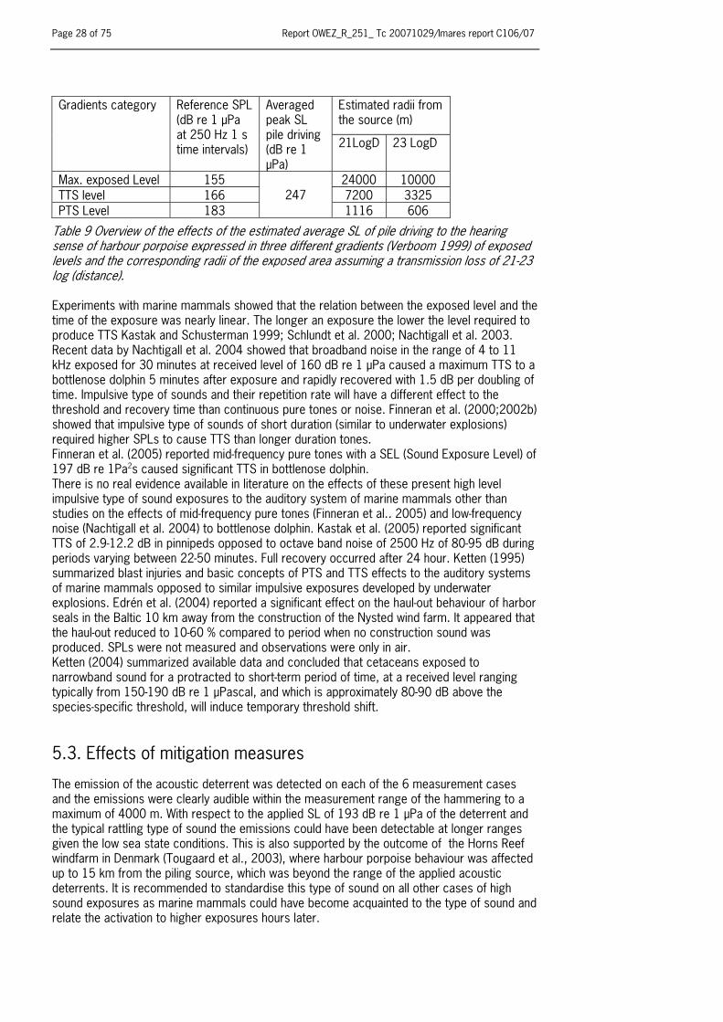
Page 28 of 75 Report OWEZ_R_251_ Tc 20071029/Imares report C106/07
Table 9 Overview of the effects of the estimated average SL of pile driving to the hearing sense of harbour porpoise expressed in three different gradients (Verboom 1999) of exposed levels and the corresponding radii of the exposed area assuming a transmission loss of 21-23 log (distance). Experiments with marine mammals showed that the relation between the exposed level and the time of the exposure was nearly linear. The longer an exposure the lower the level required to produce TTS Kastak and Schusterman 1999; Schlundt et al. 2000; Nachtigall et al. 2003. Recent data by Nachtigall et al. 2004 showed that broadband noise in the range of 4 to 11 kHz exposed for 30 minutes at received level of 160 dB re 1 μPa caused a maximum TTS to a bottlenose dolphin 5 minutes after exposure and rapidly recovered with 1.5 dB per doubling of time. Impulsive type of sounds and their repetition rate will have a different effect to the threshold and recovery time than continuous pure tones or noise. Finneran et al. (2000;2002b) showed that impulsive type of sounds of short duration (similar to underwater explosions) required higher SPLs to cause TTS than longer duration tones. Finneran et al. (2005) reported mid-frequency pure tones with a SEL (Sound Exposure Level) of 197 dB re 1Pa2s caused significant TTS in bottlenose dolphin. There is no real evidence available in literature on the effects of these present high level impulsive type of sound exposures to the auditory system of marine mammals other than studies on the effects of mid-frequency pure tones (Finneran et al.. 2005) and low-frequency noise (Nachtigall et al. 2004) to bottlenose dolphin. Kastak et al. (2005) reported significant TTS of 2.9-12.2 dB in pinnipeds opposed to octave band noise of 2500 Hz of 80-95 dB during periods varying between 22-50 minutes. Full recovery occurred after 24 hour. Ketten (1995) summarized blast injuries and basic concepts of PTS and TTS effects to the auditory systems of marine mammals opposed to similar impulsive exposures developed by underwater explosions. Edrén et al. (2004) reported a significant effect on the haul-out behaviour of harbor seals in the Baltic 10 km away from the construction of the Nysted wind farm. It appeared that the haul-out reduced to 10-60 % compared to period when no construction sound was produced. SPLs were not measured and observations were only in air. Ketten (2004) summarized available data and concluded that cetaceans exposed to narrowband sound for a protracted to short-term period of time, at a received level ranging typically from 150-190 dB re 1 μPascal, and which is approximately 80-90 dB above the species-specific threshold, will induce temporary threshold shift.
5.3. Effects of mitigation measures
The emission of the acoustic deterrent was detected on each of the 6 measurement cases and the emissions were clearly audible within the measurement range of the hammering to a maximum of 4000 m. With respect to the applied SL of 193 dB re 1 μPa of the deterrent and the typical rattling type of sound the emissions could have been detectable at longer ranges given the low sea state conditions. This is also supported by the outcome of the Horns Reef windfarm in Denmark (Tougaard et al., 2003), where harbour porpoise behaviour was affected up to 15 km from the piling source, which was beyond the range of the applied acoustic deterrents. It is recommended to standardise this type of sound on all other cases of high sound exposures as marine mammals could have become acquainted to the type of sound and relate the activation to higher exposures hours later.
Estimated radii from the source (m)
Gradients category Reference SPL (dB re 1 μPa at 250 Hz 1 s time intervals)
Averaged peak SL pile driving (dB re 1 μPa)
21LogD 23 LogD
Max. exposed Level 155 24000 10000 TTS level 166 7200 3325 PTS Level 183
247 1116 606
Report OWEZ_R_251_ Tc 20071029/Imares report C106/07 Page 29 of 75
6. Glossary of acoustic measurement terms A-D converter An arrangement of miniature transistors, available as integrated
electronic circuit (IC or CHIP), with which analogue signals are digitised.
Ambient noise The background noise in an area or environment being a composite of noise from many sources near and far. As noise normally does not contain tonal type of sounds the noise is expressed in spectral levels.
Analogue There are two main ways of arranging an electronic transfer, analogue or digital. In the analogue method, signals are continuously variable and the slightest change may be significant. Analogue circuits are subject to drift, distortion, and noise, but they are capable of handling complex signals with relatively simple circuitry.
Anthropogenic noise Collective for all human produced noise sources. Bandwidth A range of frequencies that can be passed through a channel. A
channel carrying digital information has a data rate proportional to its bandwidth.
Bit The smallest unit of data recognisable by a computer. Eight bits equals one BYTE (or 1 character).
Cetaceans Order, in taxonomic classification, which includes whales and porpoises.
Two suborders, mysticetes (baleen whales) and odontocetes (toothed whales), belong to the cetacean order.
DAC Digital to Analogue Converter. An arrangement of miniature transistors, available as integrated circuit (IC or CHIP), with which a digital signal is converted to an analogue.
Digital There are two main path of electronic signal transmission, analogue or digital. The digital method is to consider a circuit either on or off, a signal as either present or absent, with no levels in between. Electronic circuits using the digital mode are simple to design and non-critical in operation. The all-or-nothing nature of digital circuits make them immune to drift and distortion, and their simplicity makes them easy to manufacture in large quantity.
FFT Fast Fourier Transform. Transforms digitised waveforms to the frequency domain. The results can be either real or imaginary, or magnitude or phase, functions of frequency.
Hanning window Type of filter technique, used in Fast Fourier Transformed waveforms, named after its inventor von Hann, has the shape of one cycle of a cosine wave with 1 added to it so it is always positive.
Windowing is a technique used to shape the time portion of measurement data, to minimize edge effects that result in spectral leakage in the FFT spectrum. By using Window Functions correctly, the spectral resolution of the frequency-domain result will slightly decrease, but the effects of the side lobes on the result will be reduced.
Harbour porpoise Phocoena phocoena. Smallest toothed whale species occurring mostly in coastal waters and quite common in all North Sea areas. Average length 1.5 m to a maximum of 2 m.

Page 30 of 75 Report OWEZ_R_251_ Tc 20071029/Imares report C106/07
Hydrophone Device used for receiving acoustic signals underwater and converting sound vibrations to electric signals proportional to the frequency and levels of the received sound.
Pascal Unit of sound pressure level. The atmospheric pressure, i.e., the environmental air pressure in absence of sound. It is measured in a SI (Système International, i.e., International System) unit called Pascal (1 Pascal is equal to a force of 1 Newton acting on a surface of 1 square meter and is abbreviated 1 Pa). This pressure amounts to roughly 100,000 Pa (the standard value is 101,325 Pa). Then we can define sound pressure as the difference between the actual instantaneous pressure due to sound and the atmospheric pressure, measured in Pa. However, sound pressure has usually a value much smaller than the one corresponding to the atmospheric pressure. For instance, unbearably loud sounds may be around 20 Pa, while the human hearing threshold in air is around 20 μPa (μPa stands for micropascal, i.e., a unit one million times smaller than the pascal). This is much the same as the case of some gentle ripples on the surface a swimming pool. The threshold for underwater sound pressure levels is adapted to 1 μPa (See also Reference levels). Unlike the slow changes of atmospheric pressure sound pressure is rapidly changing, alternating between positive and negative values, at a rate of between 20 and 20,000 times per second. This rate is called frequency and is expressed in Hertz (abbreviated Hz), a unit equivalent to a cycle per second. In order to reduce the amount of digits, frequencies above 1,000 Hz are usually expressed in kilohertz, abbreviated kHz.
Pinger Autonomous battery powered electronic device producing sound patterns in random or constant time intervals. Developed to deter cetaceans from gillnets. Also used as reference source for hydrophone arrays or as acoustic measurements.
Pistonphone A battery-operated, precision low frequency sound source used for accurate and reliable calibration of measurement microphones and hydrophones based on the excitation of a piston inside a cylinder. The frequency is nominally 250 Hz. The hydrophone is accurately coupled to the cylinder at a fixed distance and will produce a output voltage which is accurately related to the specified or measured sound pressure level of the pistonphone. The uncertainty of the pistonphone’s sound level is nominally 0.08 dB.
Propagation losses Transmission losses of sound over distance through a medium (air, seawater). The propagation losses of sound are frequency-depended and also depend on complex number of factors (bottom structure, sediment, etc) and are mostly irregular in coastal waters. Main factors are geographical spreading (TLg ) and absorption loss
(TLa ): TL = TLg + TLa where TLg = 20 log r2 (for geometrical spherical spreading; r2 is in meters)
TLa = a r2 x 10-3 (units are dB/km)
where a is the attenuation coefficient and a function of frequency, r2 is in meters, and 10-3 is a conversion factor for m to km. The rate at which sound is absorbed by water is related to the square of frequency ( f∝α 2); lower frequency sounds have low absorption coefficients and therefore propagate long distances.
Report OWEZ_R_251_ Tc 20071029/Imares report C106/07 Page 31 of 75
Reference levels A sound level of 120 dB in air is not the same as 120 dB in water, primarily because of the differences in reference measurements. In air, the sound pressure level is referenced to 20 μPa, while in water the sound pressure level is referenced to 1 μPa. The reference conversion factor for dB air to water (dB): = 20 log (pwater/1μPa) = 20 log (20) = + 26 dB. The characteristic impedance of water is about 3600 times that of air; which equals 10 log (3600) = 36 dB. In total the conversion factor is 36+26 = 62 dB. If a jet engine produces 140 dB re 20μPa @ 1m, then the underwater equivalent sound levels would be SPLwater = SPLair + 62 = 202 dB re 1μPa.
Sample rate The value of this frequency refers to how frequently the analogue signal is measured during the digitising process. The higher the frequency the signal is sampled, the better the approximation to the original signal. The frequency defines also the aperture of the frewquency bandwidth (Bandwidth = sample rate/2). A sample rate of 512 kHz will support a frequency bandwidth up to 256 kHz. However, the higher the sample rate the more memory is required to store the samples.
SL Source level is the Sound Pressure Level of a sound source measured on the acoustic axis at a distance of 1 m from the source. In underwater acoustics this level is commonly referred to a reference pressure of 1 μPa. The definition is than 10 log intensity, divided by the reference intensity and expressed in dB (decibel) re (relative to) 1μPa at 1 m. Noise levels, although measured in different frequency bands, are always reduced to a 1 Hz frequency band and expressed as dB re 1 μPa / √ Hz.
Spectrogram A graph, which displays acoustic energy as a function of frequency allowing frequency patterns to be visualised, and reverberations to be depicted.
Spectral level Acoustic power level within a one-Hertz “slice” of a bandwidth (e.g., the spectral level at 150 Hz is the acoustic power level within the bandwidth between 149.5 Hz and 150.5 Hz).
SPL Sound Pressure Level, pressure level of a sound source measured at a certain distance from a sound source and commonly referred to a reference pressure level of 1 μPa and expressed in dB re 1 μPa.
Wenz curves Wenz curves are used as an aid to categorize the ambient noise levels as a function of ship-traffic and sea state condition.
Page 32 of 75 Report OWEZ_R_251_ Tc 20071029/Imares report C106/07
7. References Akamatsu, T., Matsusita, Y., Hatakeyama, Y. & Inoue, Y. (1996). Startle response level of the Japanese anchovy Engraulis japonicus to underwater pure tone signals. Fisheries Science 62, 648-649. Akamatsu, T., Nanami, A., & Yan, H.Y. (2003). Spotlined sardine Sardinops melanostictus listens to 1-kHz sound by using its gas bladder. Fisheries Science 69, 348-354. Andersen, S. 1970. Auditory sensitivity of the harbour porpoise Phocoena phocoena. In: G. Pilleri (ed.). Investigations on Cetacea, Vol II.- Institute of Brain Anatomy, Bern, 255-259. Anonymous 2000. Annex I, Report of the Sub-Committee on Small Cetaceans. Journal of Cetacean Research Management 2 (Suppl.), 235-245. Anonymous 2000. Horns Reef-----noise in the sea during pile-driving of a turbine foundation. Report from Tech-Wise A/S Frederica, 1-49 (in Danish). Anonymous 2001. San Fransisco-Oakland Bay Bridge, east Span Seismic Safety project, Pile Installation Demonstration Project, Fisheries Impact Assessment. PIDP EA 01208, Caltrans contract 04A0148, Task Order 205.10.90, PIDP 04-ALA-80-0.0/0.5, 1-32. Anraku, K., Matsuda, M., Shigesato, N., Nakahara, M., & Kawamura, G. (1998). Flounder show conditioned response to 200-800 Hz tone bursts despite their conditioning to 300 Hz tone-bursts. Nippon Suisan Gakkaishi, 64, 755-758. (in Japanese). Astrup, J. & Møhl, B. (1993). Detection of intense ultrasound by the cod Gadus morhua. Journal of Experimental Biology, 182, 71-80. Astrup, J. & Møhl, B. (1998). Discrimination between high and low repetition rates of ultrasonic pulses by the cod. Journal of Fish Biology, 52, 205-208. Au, W. W. L. 1993. the sonar of dolphins. Springer-Verlag, New York. Betke, K., Schultz-von Glahn, M., Matuschek, R. 2004. Underwater noise emissions from offshore wind turbines. Proc CFA/DAGA 2004, Strasbourg. Camphuysen, C. J. 2005. The return of the harbour porpoise (Phocoena phocoena) in Dutch coastal waters. Lutra, 48. Chapman, C. J. and Hawkins, A. D. 1973. A field study of hearing in cod, Gadus morhua. J. Comp. Physiol. 85, 147-167. Chapman, C. J. and Sand, O. 1974. Field studies of hearing in two species of flatfish Pleuronectes platessa (L.) and Limanda limanda (L.) (Family Pleuronectidae). Comp. Biochem. Physiol. 47A, 371-385. Degn, U. 2000. Offshore wind turbines-VVM, underwater noise measurements, analysis, and predictions. Ødegaard & Danneskiold-Samsø A/S, Rep No 00-792 rev. 1. p 1-230. Denton, E. J. and Gray, J. A. B. 1993. Stimulation of the acusto-lateralis system of clupeid fish by external sources and their own movement. Philosophical Transactions of the Royal Society of London, B. 341, 113-127.

Report OWEZ_R_251_ Tc 20071029/Imares report C106/07 Page 33 of 75
DEWI 2004. Deutsches Windenergie-Institut: Standardverfahren zur Ermittlung und Bewertung der Belastung der Meeresumwelt durch Schallimmisionen von Offshore-Windenergieanlagen. -Abschlussbericht zum Forschungsvorhaben 0327528A an das BMU, 123 pp. Edrén, S. M. E., Teilmann, J., Dietz, R., Carstensen, J. 2004. Effect from the construction of Nysted offshore wind farm on seals in Rødsand seal sanctuary based on remote video monitoring. Technical report to Energy E2 A/S. National Environmental Research Institute Roskilde. Enger, P. S. 1967. Hearing in herring. Comp. Biochem,. Phsysiol. 22, 527-538. Enger, P. S. 1981. Frequency discrimination in teleosts-central or peripheral? In: Tavolga, W. M., Popper, A. N. and Fay, R. R. (eds.). Hearing and Sound Communication in Fishes. Springer, New York, 243-255. Finneran, J. J., Schlundt, C. E., Dear, R., Carder, D. A. and Ridgway, S. H. 2002a. Auditory filter shapes for the bottlenose dolphin (Tursiops truncates) and the white whale (Delphinapterus leucas) derived with notched-noise. J. Acoust. Soc. Am. 112, 322-328. Finneran, J. J., Schlundt, C. E., Dear, R., Carder, D. A. and Ridgway, S. H. 2002b. “Temporary threshold shift in masked hearing thresholds (MTTS) in odontocetes after exposure to single underwater impulses from a seismic watergun” J. Acoustic. Soc. Am. 111, 2929-2940. Finneran, J. J., Carder, D. A., Schlundt, C. E., Dear, R. and Ridgway, S. H. 2005. Temporary threshold shift in bottlenose dolphins (Tursiops Truncaus) exposed to mid-frequency tones. J. Acoust. Soc. Am. 118 2696-2705. Fristedt, T., Morén, P., Söderberg, P. 2001. Acoustic and electro-magnetic noise induced by windmills-implications for underwater surveillance systems: pilot study. FOI-R-0233-SE. FOI, Swedish Defence Research Agency, Stockholm. Haan de, D., Burggraaf, D., Asjes, J., Lambers Hille Ris, R. 2006. Background noise measurements for MEP-NSW Baseline T0. Report nr. OWEZ_R_251_ T0 20061015. Hawkins, A. D. and Johnstone, A. D. F. 1978. The hearing of the Atlantic salmon (Salmo salar). J. Fish. Biol. 13, p 655-673. Hastings, M. C. and Popper, A. N. 2005. Effects of sound on fish. California Department of Transportation Contract 43A0139 task order, 1. http://www.dot.ca.gov/hq/env/bio/files/Effects_of_Sound_on Fish23Aug05.pdf. Ingemansson Technology AB. 2003. Utgrunden offshore wind farm-measurements of underwater noise. Report 11-00329-03012700. Ingemansson Technology A/S, Gotheburg. Kastak, D. and Schusterman, R. J. 1998. Low-frequency amphibious hearing in pinnipeds: methods, measurements, noise and ecology. J. Acoust. Soc. Am. 103, 2216-2228. Kastak, D. and Schusterman, R. J. 1999. Underwater temporary threshold shift induced by octave-band noise in three species of pinniped. J. Acoust. Soc. Am. 106, 1142-1148. Kastak, D. Southall, L., Schusterman, R. J. and Kastak, C. R. 2005. Underwater temporary threshold shift in pinnipeds: Effects of noise level and duration. J. Acoust. Soc. Am. 118, 3154-3163. Kastelein, R.A., Bunskoek, P., Hagedoorn, M., Au, W.W.L., and de Haan, D. 2002. Audiogram of a harbor porpoise (Phocoena phocoena) measured with narrow-band frequency-modulated signals, J. Acoust. Soc. Am. 112, 334-344.

Page 34 of 75 Report OWEZ_R_251_ Tc 20071029/Imares report C106/07
Kastelein, R. A., Rippe, H. T., Vaughan, N., Schooneman, N. M., Verboom, W. C., Haan, D. de, 2000. The effects of acoustic alarms on the behavior of harbor porpoises (Phocoena phocoena) in a floating pen. Marine Mammal Science, 16(1): 46-64, 2000. Kastelein, R. A., Jennings, Verboom, W. C., de Haan, D., Schooneman, N. M. 2005. Differences in the response of a striped dolphin (Stenella coeruleoalba) and a harbour porpoise (Phocoena phocoena) to an acoustic alarm. Marine Environmental Research MERE 2956. Ketten, D.R. 1995. Estimates of blast injury and acoustic trauma zones for marine mammals from underwater explosions. In: Sensory Systems of Aquatic Mammals, R. A. Kastelein, J. A. Thomas, and P. E. Nachtigall (eds.), DeSpil Publishers, pp. 391-408. Ketten, D. 2004. Marine mammal auditory systems: a summary of audiometric and anatomical data and implications for underwater acoustic impacts. International Whaling Commission, Scientific Committee (IWC-SC) Report Annex K: Standing Working Group on Environmental Concerns Report (May 2004). Submitted at the IWC56 meeting, July 2004 Knudsen, V. O., R. S. Alford, and J. W. Emling, 1948: Underwater ambient noise. J. Mar. Res., 22, 410–429. Lucke, K., Hanke, W. and Denhardt, G. 2004. Untersuchungen zum Einfluss akustischer Emissionen von Offshore-Windkraftanlagen auf marine Säuger im Bereich der Deutchen Nord-und Ostsee. Marine Warmblűter in Nord-und Ostsee: Grundlagen zur Bewertung vpon Windkraftanlagen im Offshore-Bereich. Endbericht, Teilprojekt 1, Nationalpark Schleswig-Holsteiniches Wattenmeer und Bundesministerium fűr Umwelt, Naturschutz und Reaktorsicherheit (FKZ: 0327520), 23-76. Lucke, K.,Siebert, U., Sundermeyer, J. and Benke, H. 2006. TP1- Weiterfűhrende Untersuchungen zum Einfluss akustischer Emissionen von Offshore-Windenergieanlagen auf marine Säuger im Bereich der Deutchen Nord-und Ostsee. In; Minos/Plus - Weiterfűhrende Arbeiten an Seevögeln und marine Säugern zur bewertung von Offshore Windkraftanlagen. Zweiter Zwischenbericht, April 2006. Landesamt fűr den Nationalpark Schleswig-Holsteines Wattenmeer, Tönning, 10-27. Madsen, P. T., Wahlberg, M. Tougaard, T., Lucke, K., Tyack, P. 2006. Wind turbine underwater noise and marine mammals: implications of current knowledge and data needs. Mar Ecol Prog Ser Vol. 309:279-295. Mann, D.A., Popper, A.N., & Wilson, B. (2005). Herring do not detect ultrasound. Proceedings of the Royal Society of London Biological Letters 1, 158-161. Motomatsu, K., Hiraishi, T., Yamamoto, K., & Nashimoto, K. (1998). Auditory masking by ambient noise in black rockfish Sebastes schlegeli. Nippon Suisan Gakkaishi, 64, 792-795. Nachtigall, P. E., Pawloski, J. L., AU, W. W. L., 2003. Temporary threshold shifts and recovery following noise exposure in the Atlantic bottlenosed dolphin (Tursiops truncatus). J. Acoust. Soc. Am. 113: 3425-3429. Nachtigall, P. E., Pawloski, J. L., AU, W. W. L., 2004. Temporary threshold shifts after noise exposure in the bottlenose dolphin (Tursiops truncatus) measured using evoked auditory potentials. Mar. Mamm. Sci 20 (4):673-687. Nedwell, J., Langworthy, J. and Howell, D. May 2003. Assessment of sub-sea acoustic noise and vibration from offshore wind turbines and its impact on marine wildlife; initial measurements of underwater noise during construction of offshore windfarms, and comparison with background noise.

Report OWEZ_R_251_ Tc 20071029/Imares report C106/07 Page 35 of 75
Nedwell, J., Howell, D. Oct 2004. A review of offshore windfarm related underwater noise sources. Report No. 544 R0308. Nystuen, J. A. and Farmer, D. M. 1987: The influence of wind of the underwater sound generated by light rain, J. Acoust. Soc. Am., 82, 270-274. Otani, S., Naito, Y., Kato, A. and Kawamura, A., 2001. Oxygen consumption and swim speed of the harbor porpoise Phocoena phocoena. Fisheries Science Volume 67 Issue 5 Page 894-898, October 2001 Popov, V. V., Ladygina, T. F. and Supin, A. Ya. 1986. Evoked potential of the auditory cortex of the porpoise, Phocoena phocoena. J. Comp. Physiol. 158, 705-711. Richardson, W. J., Green, C. R. G. jr., Malme, C. I. and Thomson, D. H. 1995. Marine Mammals and Noise. Academic Press, San Diego, 576 pp. Schlundt, C. E., Finneran, J. J., Carder, D. A., Ridgway, S. H. 2000. Temporary shift in masked hearing thresholds of bottlenose dolphins, Turchiops truncatus and white whales, Delphinapterus leucas, after exposure to intense tones. J. Acoust. Soc. Am. 107:3496-3508. Sparling, C. E. (2003). Causes and consequences of variation in the energy expenditure of grey seals (Halichoerus grypus). PhD Thesis, University of St Andrews, Scotland, UK. Terhune, J. and Turnbull, S. 1995. Variation in the psychometric functions and hearing thresholds of a harbour seal. In Kastelein, R. A., Thomas, J. A. and Nachtigall, P. E. (eds), Sensory systems of aquatic mammals. De Spil Publ., Woerden, Netherlands, 81-93. Tougaard, J., Carstensen, J., Teilmann, J., Bech N., 2003. Short-term effects of the construction of wind turbines on harbour porpoises at Horns Reef. Tech. Rep. HME/362-02662, to: TechWise A/S., Hedeselskabet, Roskilde. Tougaard, J., Carstensen, J., Wisch, M. S., Teilmann, J., Bech N., Shokv, H., Hendriksen, O. D. 2005. Harbour porpoises on Horns reef-effects of the Horns reef Wind farm. Annual Status Report 2004 to Elsam. NERI, Roskilde. Turnpenny, A. W. H. & Nedwell, J. R. (1994). The effects on marine fish, diving animals and birds of underwater sound generated by seismic surveys. Report to the UK offshore Operators Association, No FRR 089/94. Tyack, P. 1998. Acoustic communication under the sea. In: Hopp S. L., Owren M. J., Evans, C. S. (eds). Animal acoustic communication: recent technical advances. Springer-Verlag, Heidelberg, p-163-220. Urick, R. J. 1983. Principles of underwater sound for engineers. McGraw-Hill book Company. Verboom, W. C., 1992. Bio Acoustics: Standardization, reference levels and data notation for underwater sound measure. P. 741-751 In: J. A. Thomas, R. A. Kastelein and A.Ya. Supin, Marine Mammal Sensory systems. Plenum New York. 773 p. Verboom, W. C. 1999. Intense Sound Levels and Marine Mammals. TNO-report HAG-RPT-9900001 56 p. Wahlberg, M., Westerberg, H. 2005. Hearing in fish and their reaction to sounds from offshore wind farms. Mar. Ecol. Prog. Ser. 288:295-309. Westerberg, H. 1994. Fiskeriundersökningar vid havsbaserat vindkraftwerk 1990-1993. Rapp 5-1994. Fiskeriverket, Utredningskontoret Jönköping.

Page 36 of 75 Report OWEZ_R_251_ Tc 20071029/Imares report C106/07
Wenz curves (1962). Reprinted with permission from National Research Council. 2003. Ocean Noise and Marine Mammals. National Academy Press, Washington, D.C. (as adapted from Wenz, 1962) by the National Academy of Sciences. Yan H. Y., Fine M. L., Horn N. S., Colón W. E. 2000. Variability in the role of gasbladder in fish audition. Journal of Comparative Physiology, Vol. 186, 435-445. Yelverton, J. T., Richmond, D. R., Fletcher, E. R. And Jones, R.K., 1973. Safe distances from underwater explosions for mammals and birds. DNA 3114T. Rep. from Lovelace Foundation fro medical Educ. and Res., Albuquerque, NM, for Defense Nuclear agency, Washington, DC 67 p. NTIS AD-766952. Yelverton, J. T. 1981. Underwater explosion damage risk criteria for fish, birds and mammals. Manuscript, presented on the 102nd Meet. Acoust. Soc. Am. Miami beach, Fl, Dec. 1981. 32 p.

Report OWEZ_R_251_ Tc 20071029/Imares report C106/07 Page 37 of 75
8. Figures Figure 3 The building of the Off-Shore Wind farm Egmond aan Zee (OWEZ) in the Dutch coastal zone 8 - 18 km of the coast of Egmond aan Zee with 36 wind turbines with a total capacity of 108 MW.

Page 38 of 75 Report OWEZ_R_251_ Tc 20071029/Imares report C106/07
Figure 4 Auditory threshold levels versus frequency of Atlantic salmon (Salmo salar) (Hawkins and Johnson 1978), Atlantic cod (Chapman and Hawkins 1973), Atlantic herring (Enger 1967), and dab (Chapman and Sand 1974). For comparison the auditory threshold of pacific herring (Mann et al. 2005 is included. The threshold curves clearly show the effects of species provided with a swimbladder (cod) and those that are not (dab). Although not all selected fish species with swimbladder has a low hearing threshold. In a recent publication the role of the swimbladder serving as an auditory enhancement was doubted in relation to bony fish that are not provided with a Weberian Ossicles or Apparatus, a connection between swimbladder and inner ear (Yan et al. 2000).
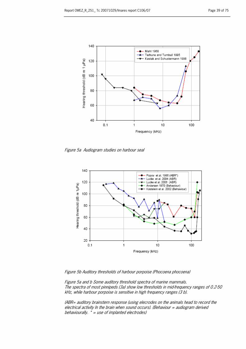
Report OWEZ_R_251_ Tc 20071029/Imares report C106/07 Page 39 of 75
Figure 5a Audiogram studies on harbour seal Figure 5b Auditory thresholds of harbour porpoise (Phocoena phocoena) Figure 5a and b Some auditory threshold spectra of marine mammals. The spectra of most pinnipeds (3a) show low thresholds in mid-frequency ranges of 0.2-50 kHz, while harbour porpoise is sensitive in high frequency ranges (3 b). (ABR= auditory brainstern response (using elecrodes on the animals head to record the electrical activity In the brain when sound occurs). (Behaviour = audiogram derived behaviourally. * = use of implanted electrodes)

Page 40 of 75 Report OWEZ_R_251_ Tc 20071029/Imares report C106/07
Figure 6 Measurement locations of hammering cases with monopile 1 as the most southern location (yellow), monopile 10 (magenta), monopile 13 to the south (red), monopile 22 to the south (green), monopile 34 (black) to the north and monopile 36 (orange) as most northern location. Close to the monopile 36 locations the Q8B gas rig station as situated.
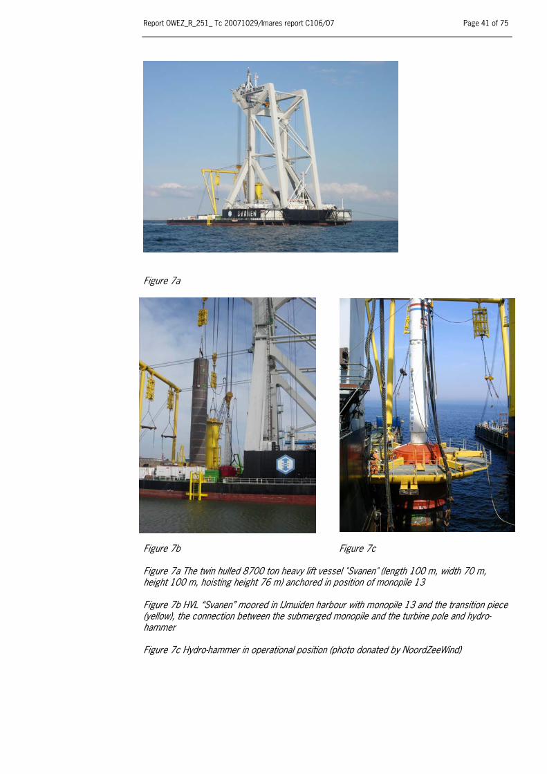
Report OWEZ_R_251_ Tc 20071029/Imares report C106/07 Page 41 of 75
Figure 7a
Figure 7b Figure 7c Figure 7a The twin hulled 8700 ton heavy lift vessel "Svanen" (length 100 m, width 70 m, height 100 m, hoisting height 76 m) anchored in position of monopile 13 Figure 7b HVL “Svanen” moored in IJmuiden harbour with monopile 13 and the transition piece (yellow), the connection between the submerged monopile and the turbine pole and hydro-hammer Figure 7c Hydro-hammer in operational position (photo donated by NoordZeeWind)

Page 42 of 75 Report OWEZ_R_251_ Tc 20071029/Imares report C106/07
0 5 10 15 20 25 30 35
Pile nr
0
500
1000
1500
2000
2500
Tota
l Ene
rgy
[MJo
ule]
0
2000
4000
6000
8000
Tota
l nr B
low
s
Total blowsTotal energyTotal blows MEnergy MAvg total blowsAvg total energy
Overview of hammering energy
Figure 8 Overview of applied energy ( MJoule) and total number of hammering blows marked M for the 6 measurement cases (100 % filling) and the other 30 hammering cases, which were not measured. Average lines are given for the cases which were not measured. The overview shows that the selection of measurement cases was representative for the applied energy in all hammering cases and that the case with highest applied energy (monopile 34) was actually measured. No data was available for hammering case 24
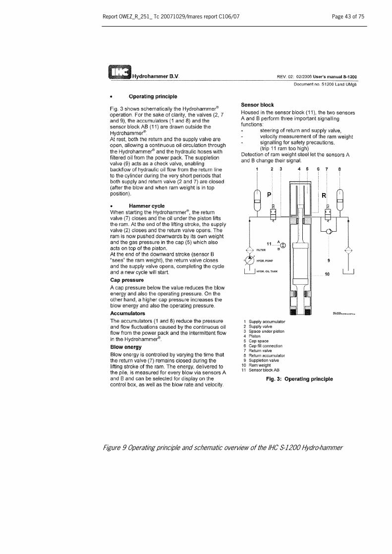
Report OWEZ_R_251_ Tc 20071029/Imares report C106/07 Page 43 of 75
Figure 9 Operating principle and schematic overview of the IHC S-1200 Hydro-hammer

Page 44 of 75 Report OWEZ_R_251_ Tc 20071029/Imares report C106/07
WCW WindCat 4 Workboat in action
WindCat Marine B.V. Trawlerkade 106 1976 CC IJmuiden
Telephone. :+31 255 5138 39 Telefax. :+31 255 5120 95
Website: www.windcatworkboats.com
Technical specifications Year of building :2005 Construction :Aluminium Propulsion :2 x Volvo D12 ZF gearboxes driving Hamilton jets with foils Maximum speed :30 knots Length o.a. : 15 m Beam : 6,10 m Depth : 0.9 m Accommodation :12 persons Classification :MCA category 2 up to 60 miles with 12 passengers Electronics :2 Plotters, 2 GPS receivers, auto-pilot, 2 VHF systems.
Figure 10 Particulars and overview of the Windcat 4 workboat

Report OWEZ_R_251_ Tc 20071029/Imares report C106/07 Page 45 of 75
0.1 1 10 100 1000 10000 100000Frequency (Hz)
-30
-20
-10
0
10
20
30
Gai
n (d
B)
Gain 0 dB 1 Hz
Gain 0 dB 10 Hz
Gain 10 dB 1 Hz
Gain 20 dB 1 Hz
Gain 20 dB 10 Hz
Gain 10 dB 10 Hz
Calibration A1101 May 2006
Response curve ETEC A1101 pre-amplifier Figure 11 Response curve of the ETEC A1101 amplifier with a 1 and 10 Hz high-pas filter setting and the 150 kHz low-pass filter. The response was measured with a 100 mV (p/p) sine wave reference signal in the range of 0.1 Hz to 250 kHz from a HP33120A arbitrary waveform generator and the output signal of the A1101 amplifier was measured with Tektronix 455 oscilloscope. In the frequency band of interest (10Hz-10 KHz) at 0 and 10 dB gain setting the response of the pre-amplifier is flat.

Page 46 of 75 Report OWEZ_R_251_ Tc 20071029/Imares report C106/07
Figure 12 Hydrophone RESON TC 4033 response curve
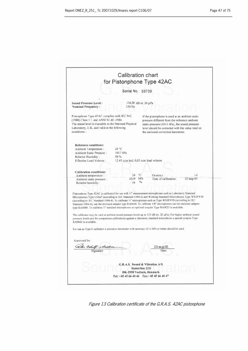
Report OWEZ_R_251_ Tc 20071029/Imares report C106/07 Page 47 of 75
Figure 13 Calibration certificate of the G.R.A.S. 42AC pistonphone

Page 48 of 75 Report OWEZ_R_251_ Tc 20071029/Imares report C106/07
Figure 14 Hydrophone calibration set-up with left the Reson hydrophone TC4032 coupled onto the G.R.A.S. 42 AC pistonphone and the sound level meter type B&K 2239 coupled onto the side gate of the coupler. On the right side the calibration equipment to the right the 10 kHz Ducane NetMark 1000 pinger used as reference source during the measurements.
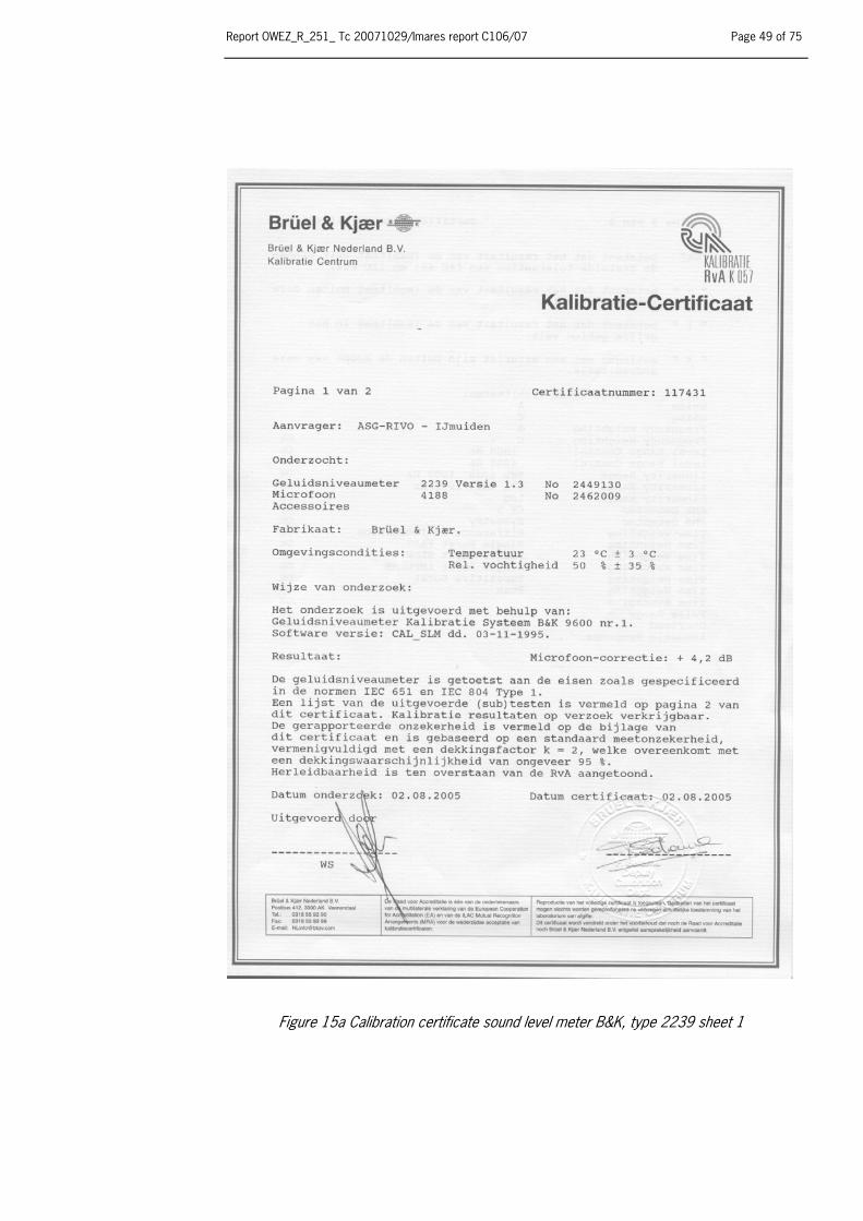
Report OWEZ_R_251_ Tc 20071029/Imares report C106/07 Page 49 of 75
Figure 15a Calibration certificate sound level meter B&K, type 2239 sheet 1
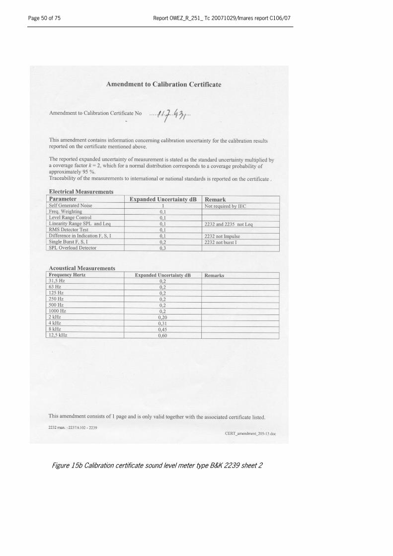
Page 50 of 75 Report OWEZ_R_251_ Tc 20071029/Imares report C106/07
Figure 15b Calibration certificate sound level meter type B&K 2239 sheet 2

Report OWEZ_R_251_ Tc 20071029/Imares report C106/07 Page 51 of 75
Figure 16 Accuracy of GPS positions over a period of 4 days. Position data received from a GM 17N GPS receiver on top of the roof of the Wageningen IMARES laboratory, October 2005. The grid size is 3.81 m latitude (in the direction of the red arrow) and 2.41 m longitude. The maximum deviation to the average position is 3 divisions, which equals to 11.7 m and 7.23 m.

Page 52 of 75 Report OWEZ_R_251_ Tc 20071029/Imares report C106/07
4.2 4.22 4.24 4.26 4.28Time [sec]
-0.05
-0.025
0
0.025
0.05
Am
plitu
de [V
]
Monopile 1Peakamplitude
(2653 m case 8.1)
21.8 21.825 21.85 21.875Time [sec]
-0.075
-0.05
-0.025
0
0.025
0.05
0.075
Am
plitu
de [V
]
Peakamplitude
Monopile 1 (2653 m case 8.2)
Figure 17 Overview of time history of two successive blow signals measured at 2653 m during the hammering of monopile 10 labelled as case 8.1 and 8.2. The overview clarifies that a time window of 0.06 s would be too short to include the complete pulse period (8.1) and secondly it missed the highest amplitude (8.2). Based on this observation in the analysis the data set was re-processed with a time window of 0.1 s.
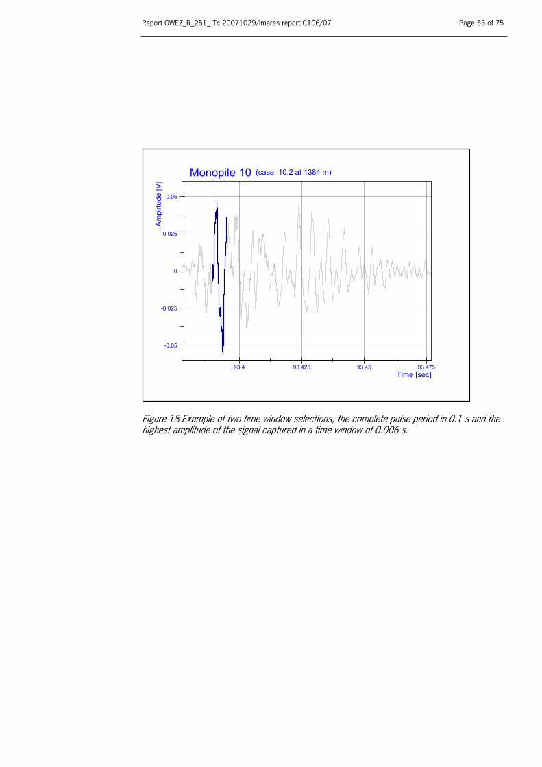
Report OWEZ_R_251_ Tc 20071029/Imares report C106/07 Page 53 of 75
93.4 93.425 93.45 93.475Time [sec]
-0.05
-0.025
0
0.025
0.05
Am
plitu
de [V
]
Monopile 10 (case 10.2 at 1384 m)
Figure 18 Example of two time window selections, the complete pulse period in 0.1 s and the highest amplitude of the signal captured in a time window of 0.006 s.
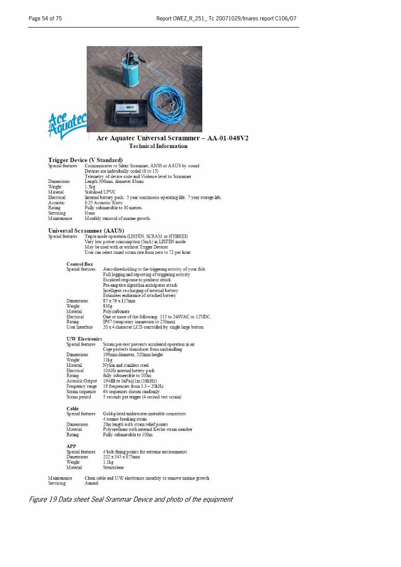
Page 54 of 75 Report OWEZ_R_251_ Tc 20071029/Imares report C106/07
Figure 19 Data sheet Seal Srammar Device and photo of the equipment
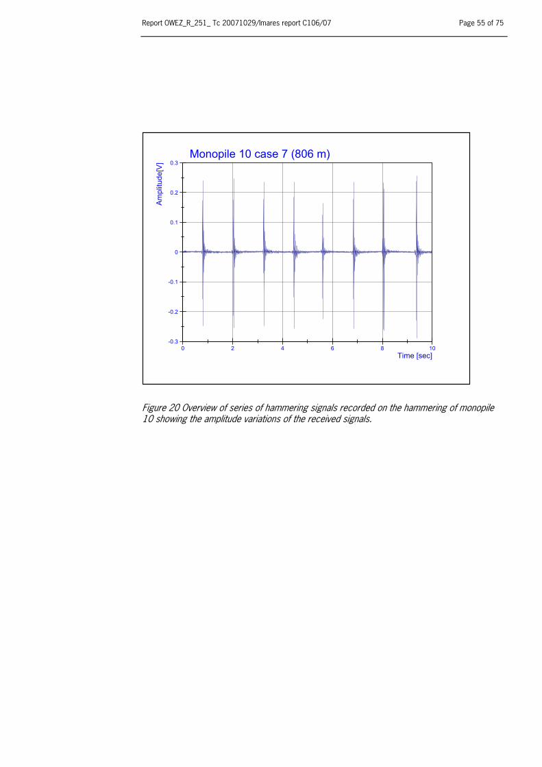
Report OWEZ_R_251_ Tc 20071029/Imares report C106/07 Page 55 of 75
0 2 4 6 8 10Time [sec]
-0.3
-0.2
-0.1
0
0.1
0.2
0.3A
mpl
itude
[V]
Monopile 10 case 7 (806 m)
Figure 20 Overview of series of hammering signals recorded on the hammering of monopile 10 showing the amplitude variations of the received signals.
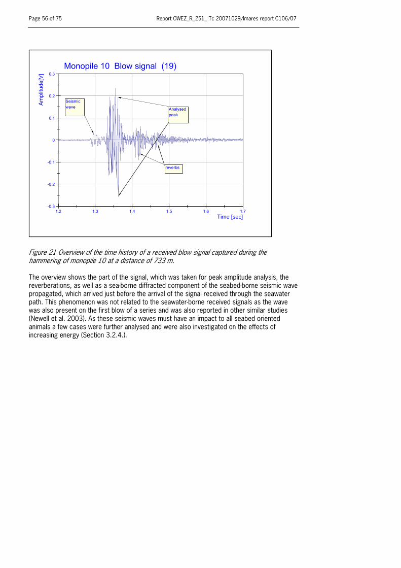
Page 56 of 75 Report OWEZ_R_251_ Tc 20071029/Imares report C106/07
1.2 1.3 1.4 1.5 1.6 1.7Time [sec]
-0.3
-0.2
-0.1
0
0.1
0.2
0.3
Am
plit u
de[V
]
Monopile 10 Blow signal (19)
Seismicwave Analysed
peak
reverbs
Figure 21 Overview of the time history of a received blow signal captured during the hammering of monopile 10 at a distance of 733 m. The overview shows the part of the signal, which was taken for peak amplitude analysis, the reverberations, as well as a sea-borne diffracted component of the seabed-borne seismic wave propagated, which arrived just before the arrival of the signal received through the seawater path. This phenomenon was not related to the seawater-borne received signals as the wave was also present on the first blow of a series and was also reported in other similar studies (Newell et al. 2003). As these seismic waves must have an impact to all seabed oriented animals a few cases were further analysed and were also investigated on the effects of increasing energy (Section 3.2.4.).
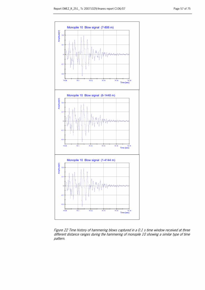
Report OWEZ_R_251_ Tc 20071029/Imares report C106/07 Page 57 of 75
74.08 74.1 74.12 74.14 74.16 74.18Time [sec]
-0.2
-0.1
0
0.1
0.2
Am
plitu
de[V
]
Monopile 10 Blow signal (7-806 m)
74.08 74.1 74.12 74.14 74.16 74.18Time [sec]
-0.2
-0.1
0
0.1
0.2
Am
plitu
de[V
]
Monopile 10 Blow signal (1-4144 m)
74.08 74.1 74.12 74.14 74.16 74.18Time [sec]
-0.2
-0.1
0
0.1
0.2
Am
p litu
de[V
]
Monopile 10 Blow signal (6-1448 m)
Figure 22 Time history of hammering blows captured in a 0.1 s time window received at three different distance ranges during the hammering of monopile 10 showing a similar type of time pattern.

Page 58 of 75 Report OWEZ_R_251_ Tc 20071029/Imares report C106/07
33.8 33.825 33.85 33.875 33.9Time [sec]
-0.3
-0.2
-0.1
0
0.1
0.2
0.3
Am
plitu
de[ V
]
Monopile 34 Blow signal (2-726 m)
19.62 19.64 19.66 19.68 19.7 19.72Time [sec]
-0.15
-0.1
-0.05
0
0.05
0.1
0.15
Am
plitu
de[V
]
Monopile 34 Blow signal (3-1326 m)
55.8 55.825 55.85 55.875Time [sec]
-0.06
-0.04
-0.02
0
0.02
0.04
0.06
Am
plitu
de[V
]
Monopile 34 Blow signal (5-3658 m)
Figure 23 Time history of hammering blows captured in a 0.1 s time window received at three different distance ranges during the hammering of monopile 34 showing an irregular time pattern with the signal peaking at the aft part of the signal at longest distance.

Report OWEZ_R_251_ Tc 20071029/Imares report C106/07 Page 59 of 75
Monopile 13
15 17.5 20 22.5 25 27.5 30Penetration [m]
140
150
160
170
180
190
200
SPL
[dB
re 1
µPa
(rm
s)]
0
200
400
600
800
Ene
rgy
[kJo
ule ]
Energy
SPL broad 0.006
SPL peak 0.006
2367 m2350 m
3652 m
1486 m
1514 m
3145 m
2382 m2294 m
3034 m
Figure 24 Graph of broad-band Sound Pressure Levels (SPL) of the highest amplitude and blow energy developed on the hammering of monopile 13 as a function of the penetration depth. The SPLbroad results are the broadband levels measured with a time window of 0.006 s over the highest amplitude. The SPL peak value represents the highest peak SPL after FFT. The SPLs of series measured in the 2300 m distance range are in close range, the applied blow energy in this part of the cycle was more or less constant. The listed Standard Deviation is the maximum deviation found over the number of blows per data series. The small differences between peak levels and broad band levels measured over the highest peak (6 ms cases) indicate the energy peaked in a narrow frequency band. Data
series
Cases Penetration Energy Distance
SPL broad (0.1s)
SPL peak (0.1s)
SPL broad (0.006s)
SPL peak (0.006s)
(nr) (nr) (m) (kJ) (m) [dB re 1 μPa (rms)] (StDev) 1 7 15.5 65 1487 174 (1.3) 170 (1.5) 179 (1.6) 179 (1.6) 2 11 20.25 126 1514 178 (1.3) 172 (2.2) 184 (1.5) 184 (1.9) 3 7 22.25 480 3652 160 (0.6) 152 (0.6) 164 (1.0) 163 (1.4) 4 11 23.5 578 2382 170 (0.8) 161 (1.7) 174 (1.1) 174 (0.9) 5 8 24 577 2367 169 (1.3) 161 (2.2) 173 (1.7) 170 (4.0) 6 11 24.5 578 2350 169 (0.7) 161 (1.3) 172 (1.7) 172 (2.4) 7 14 25 576 2294 170 (1.0) 162 (1.4) 175 (1.8) 175 (3.1) 8 6 27 674 3145 157 (0.9) 147 (1.6) 161 (0.7) 158 (2.1) 9 10 27.25 707 3034 159 (0.6) 151 (0.9) 163 (1.5) 161 (2.7)
StDev max 1.3 2.2 1.8 4.0

Page 60 of 75 Report OWEZ_R_251_ Tc 20071029/Imares report C106/07
500 750 1000 2500 5000Distance [m]
140
150
160
170
180
190
200
SPL
[dB
re 1
µPa
Vrm
s]
SPL broad 0.006 s
SPL peak 0.006 s
Monopile 13
2
1
3
4
56
7
8
9
Figure 25 Graph with broad-band Sound Pressure Levels (SPL) as a function of the hydrophone distance from the location of monopile 13. The SPLbroad results are the broadband levels measured with a time window of 0.006 s over the highest amplitude. The SPL peak value represents the highest peak SPL after FFT. The differences between peak levels and broad band levels are minor with exceptions in the higher energy range. The differences between the results of the first and second series at similar distance indicate the effect of the different angle of the first location and the other positions (Figure 6). Data
series
Cases Penetration Energy Distance
SPL broad (0.1s)
SPL peak (0.1s)
SPL broad (0.006s)
SPL peak (0.006s)
(nr) (nr) (m) (kJ) (m) [dB re 1 μPa (rms)] (StDev) 1 7 15.5 65 1487 174 (1.3) 170 (1.5) 179 (1.6) 179 (1.6) 2 11 20.25 126 1514 178 (1.3) 172 (2.2) 184 (1.5) 184 (1.9) 3 7 22.25 480 3652 160 (0.6) 152 (0.6) 164 (1.0) 163 (1.4) 4 11 23.5 578 2382 170 (0.8) 161 (1.7) 174 (1.1) 174 (0.9) 5 8 24 577 2367 169 (1.3) 161 (2.2) 173 (1.7) 170 (4.0) 6 11 24.5 578 2350 169 (0.7) 161 (1.3) 172 (1.7) 172 (2.4) 7 14 25 576 2294 170 (1.0) 162 (1.4) 175 (1.8) 175 (3.1) 8 6 27 674 3145 157 (0.9) 147 (1.6) 161 (0.7) 158 (2.1) 9 10 27.25 707 3034 159 (0.6) 151 (0.9) 163 (1.5) 161 (2.7)
StDev max 1.3 2.2 1.8 4.0

Report OWEZ_R_251_ Tc 20071029/Imares report C106/07 Page 61 of 75
Monopile 1
7.5 10 12.5 15 17.5 20 22.5Penetration [m]
140
150
160
170
180
190
200
SPL
[dB
re 1
µPa
(rm
s)]
0
200
400
600
800
1000
Ene
rgy
[kJo
ule ]
Energy
SPL broad 0.006
SPL peak 0.006
2237 m
2254 m 2155 m
2368 m
2346 m
2526 m2641 m
2652 m
Figure 26 Graph of broad-band Sound Pressure Levels (SPL) of the highest amplitude and blow energy developed on the hammering of monopile 1 as a function of the penetration depth. The SPLbroad results are the broadband levels measured with a time window of 0.006 s over the highest amplitude. The SPL peak value represents the highest peak SPL after FFT. The graph shows that the SPL’s measured at the start of the hammering cycle with low energy ratings (67 kJoule) were in the same range of those measured with highest blow energy. The differences between peak levels and broad band levels are minor in most 6 ms cases indicating the energy peaked in a narrow frequency band. Data
series
Cases Penetration Energy Distance
SPL broad (0.1s)
SPL peak (0.1s)
SPL broad (0.006s)
SPL peak (0.006s)
(nr) (nr) (m) (kJ) (m) [dB re 1 μPa (rms)] (StDev) 1 7 9.75 67 2368 158 (1.4) 149 (1.7) 164 (1.5) 162 (1.4) 5 7 13.65 563 2237 163 (0.2) 154 (1.7) 170 (0.4) 169 (0.9) 6 11 13.9 593 2346 171 (0.7) 163 (1.9) 177 (0.6) 177 (0.7) 7 13 14.65 587 2254 161 (0.8) 151 (1.1) 166 (1.3) 162 (1.4) 8 13 16.15 703 2156 161 (0.5) 149 (1.1) 167 (1.0) 163 (1.4) 9 15 18.4 829 2641 158 (0.4) 147 (1.1) 165 (1.9) 161 (1.6) 10 12 19.9 838 2526 161 (0.5) 149 (2.6) 168 (0.8) 163 (0.9) 13 9 21.9 802 2653 168 (1.1) 159 (1.8) 171 (1.6) 170 (2.3)
StDev max 1.4 2.6 1.6 2.3

Page 62 of 75 Report OWEZ_R_251_ Tc 20071029/Imares report C106/07
10001000 2000 3000 4000 5000Distance [m]
140
150
160
170
180
190
200
SPL
[dB
re 1
µPa
(rm
s)]
SPL broad 0.006
SPL peak 0.006
Monopile 1
8
5
7
6
1 10
9
13
Figure 27 Graph with broad-band Sound Pressure Levels (SPL) as a function of the hydrophone distance from the location of monopile 1. The SPLbroad results are the broadband levels measured with a time window of 0.006 s over the highest amplitude. The SPL peak value represents the highest peak SPL after FFT. The SPL results are the broadband levels measured with a time window of 0.006 s over the part with the highest amplitude as well as the Fast Fourier transformed result of the SPL of the highest frequency of the spectrum (blocksize 3077 samples). When values of broad band and peak levels are close it indicates that the energy peaked in a narrow band, when peak levels are much lower it implicates that energy was also detected in a broader frequency band. The position of the measurements of data series 13 was at a different angle compared to the other locations. Data
series
Cases Penetration Energy Distance
SPL broad (0.1s)
SPL peak (0.1s)
SPL broad (0.006s)
SPL peak (0.006s)
(nr) (nr) (m) (kJ) (m) [dB re 1 μPa (rms)] (StDev) 1 7 9.75 67 2368 158 (1.4) 149 (1.7) 164 (1.5) 162 (1.4) 5 7 13.65 563 2237 163 (0.2) 154 (1.7) 170 (0.4) 169 (0.9) 6 11 13.9 593 2346 171 (0.7) 163 (1.9) 177 (0.6) 177 (0.7) 7 13 14.65 587 2254 161 (0.8) 151 (1.1) 166 (1.3) 162 (1.4) 8 13 16.15 703 2156 161 (0.5) 149 (1.1) 167 (1.0) 163 (1.4) 9 15 18.4 829 2641 158 (0.4) 147 (1.1) 165 (1.9) 161 (1.6) 10 12 19.9 838 2526 161 (0.5) 149 (2.6) 168 (0.8) 163 (0.9) 13 9 21.9 802 2653 168 (1.1) 159 (1.8) 171 (1.6) 170 (2.3)
StDev max 1.4 2.6 1.6 2.3
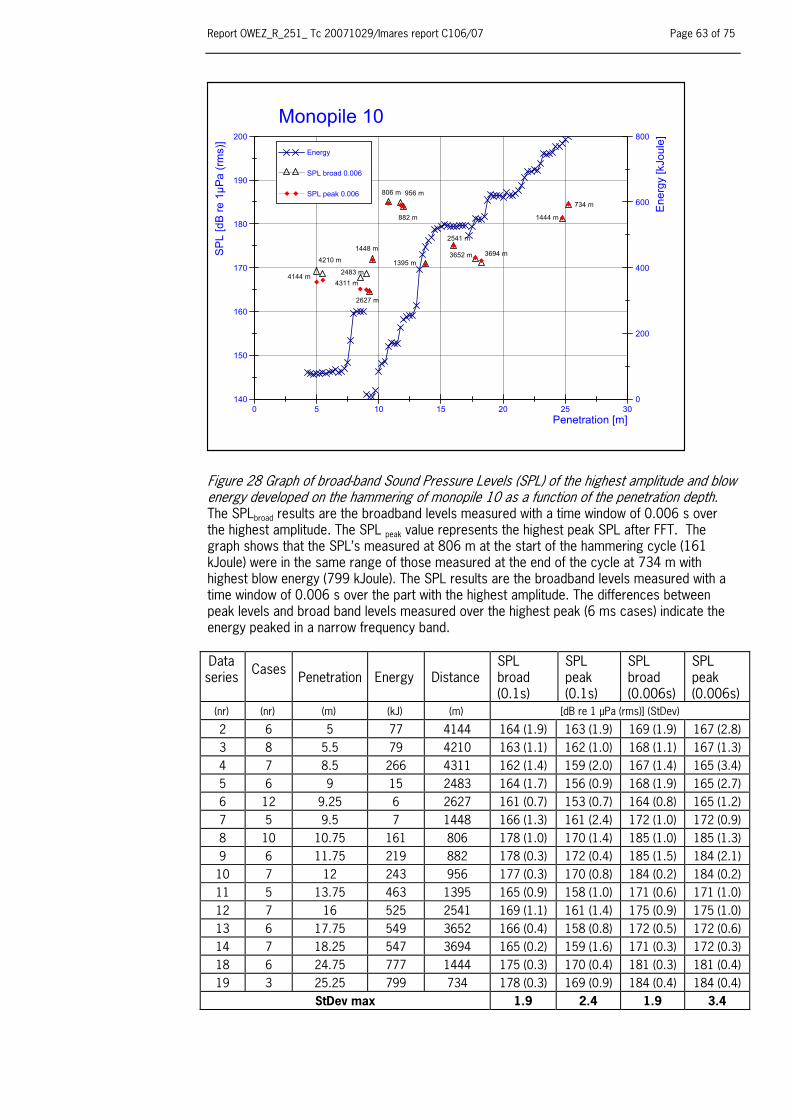
Report OWEZ_R_251_ Tc 20071029/Imares report C106/07 Page 63 of 75
Monopile 10
0 5 10 15 20 25 30Penetration [m]
140
150
160
170
180
190
200
SPL
[dB
r e 1
µPa
(rm
s)]
0
200
400
600
800
Ene
rgy
[kJo
ule]
Energy
SPL broad 0.006
SPL peak 0.006
2627 m
1448 m
4311 m4144 m
4210 m
882 m
2483 m
806 m 956 m
1395 m
2541 m
3652 m 3694 m
1444 m
734 m
Figure 28 Graph of broad-band Sound Pressure Levels (SPL) of the highest amplitude and blow energy developed on the hammering of monopile 10 as a function of the penetration depth. The SPLbroad results are the broadband levels measured with a time window of 0.006 s over the highest amplitude. The SPL peak value represents the highest peak SPL after FFT. The graph shows that the SPL’s measured at 806 m at the start of the hammering cycle (161 kJoule) were in the same range of those measured at the end of the cycle at 734 m with highest blow energy (799 kJoule). The SPL results are the broadband levels measured with a time window of 0.006 s over the part with the highest amplitude. The differences between peak levels and broad band levels measured over the highest peak (6 ms cases) indicate the energy peaked in a narrow frequency band. Data
series
Cases Penetration Energy Distance
SPL broad (0.1s)
SPL peak (0.1s)
SPL broad (0.006s)
SPL peak (0.006s)
(nr) (nr) (m) (kJ) (m) [dB re 1 μPa (rms)] (StDev) 2 6 5 77 4144 164 (1.9) 163 (1.9) 169 (1.9) 167 (2.8) 3 8 5.5 79 4210 163 (1.1) 162 (1.0) 168 (1.1) 167 (1.3) 4 7 8.5 266 4311 162 (1.4) 159 (2.0) 167 (1.4) 165 (3.4) 5 6 9 15 2483 164 (1.7) 156 (0.9) 168 (1.9) 165 (2.7) 6 12 9.25 6 2627 161 (0.7) 153 (0.7) 164 (0.8) 165 (1.2) 7 5 9.5 7 1448 166 (1.3) 161 (2.4) 172 (1.0) 172 (0.9) 8 10 10.75 161 806 178 (1.0) 170 (1.4) 185 (1.0) 185 (1.3) 9 6 11.75 219 882 178 (0.3) 172 (0.4) 185 (1.5) 184 (2.1) 10 7 12 243 956 177 (0.3) 170 (0.8) 184 (0.2) 184 (0.2) 11 5 13.75 463 1395 165 (0.9) 158 (1.0) 171 (0.6) 171 (1.0) 12 7 16 525 2541 169 (1.1) 161 (1.4) 175 (0.9) 175 (1.0) 13 6 17.75 549 3652 166 (0.4) 158 (0.8) 172 (0.5) 172 (0.6) 14 7 18.25 547 3694 165 (0.2) 159 (1.6) 171 (0.3) 172 (0.3) 18 6 24.75 777 1444 175 (0.3) 170 (0.4) 181 (0.3) 181 (0.4) 19 3 25.25 799 734 178 (0.3) 169 (0.9) 184 (0.4) 184 (0.4)
StDev max 1.9 2.4 1.9 3.4

Page 64 of 75 Report OWEZ_R_251_ Tc 20071029/Imares report C106/07
1 10 100 1000 10000
Distance [m]
150
175
200
225
250
275
SP
L [d
B re
1 µ
Pa
(rm
s )]
SPl broad 0.006
Regress SPL 0.006
SPL broad 0.1
Regress SPL 0.1
MONOPILE 10
Regression function249.147969670947-22.7318760676539log(X)
Regression function235.878660160267-20.4070806098012log(X)
Figure 29 Graph with broad-band Sound Pressure Levels (SPL) as a function of the hydrophone distance from the location of monopile 10 and the calculated regression. Graph of SPL broad band results of a time window of 0.006 s covering the peak amplitude and the SPL result over the complete pulse cycle in a time averaging window of 0.1 s with the calculation of the log regression of both cases resulting in the Source Level value and propagation losses factor as calculated result (SL broad 0.1 s 235.88-20.41log (Distance) and SL broad 0.006 s 249.15-22.73log(Distance). The plotted data involve all processed blow cases per distance sequence (FFT nr blows). The listed Standard Deviation is the maximum deviation found of the calculation over the number of blows per data series. Data
series
Cases Penetration Energy Distance
SPL broad (0.1s)
SPL peak (0.1s)
SPL broad (0.006s)
SPL peak (0.006s)
(nr) (nr) (m) (kJ) (m) [dB re 1 μPa (rms)] (StDev) 2 6 5 77 4144 164 (1.9) 163 (1.9) 169 (1.9) 167 (2.8) 3 8 5.5 79 4210 163 (1.1) 162 (1.0) 168 (1.1) 167 (1.3) 4 7 8.5 266 4311 162 (1.4) 159 (2.0) 167 (1.4) 165 (3.4) 5 6 9 15 2483 164 (1.7) 156 (0.9) 168 (1.9) 165 (2.7) 6 12 9.25 6 2627 161 (0.7) 153 (0.7) 164 (0.8) 165 (1.2) 7 5 9.5 7 1448 166 (1.3) 161 (2.4) 172 (1.0) 172 (0.9) 8 10 10.75 161 806 178 (1.0) 170 (1.4) 185 (1.0) 185 (1.3) 9 6 11.75 219 882 178 (0.3) 172 (0.4) 185 (1.5) 184 (2.1) 10 7 12 243 956 177 (0.3) 170 (0.8) 184 (0.2) 184 (0.2) 11 5 13.75 463 1395 165 (0.9) 158 (1.0) 171 (0.6) 171 (1.0) 12 7 16 525 2541 169 (1.1) 161 (1.4) 175 (0.9) 175 (1.0) 13 6 17.75 549 3652 166 (0.4) 158 (0.8) 172 (0.5) 172 (0.6) 14 7 18.25 547 3694 165 (0.2) 159 (1.6) 171 (0.3) 172 (0.3) 18 6 24.75 777 1444 175 (0.3) 170 (0.4) 181 (0.3) 181 (0.4) 19 3 25.25 799 734 178 (0.3) 169 (0.9) 184 (0.4) 184 (0.4)
StDev max 1.9 2.4 1.9 3.4
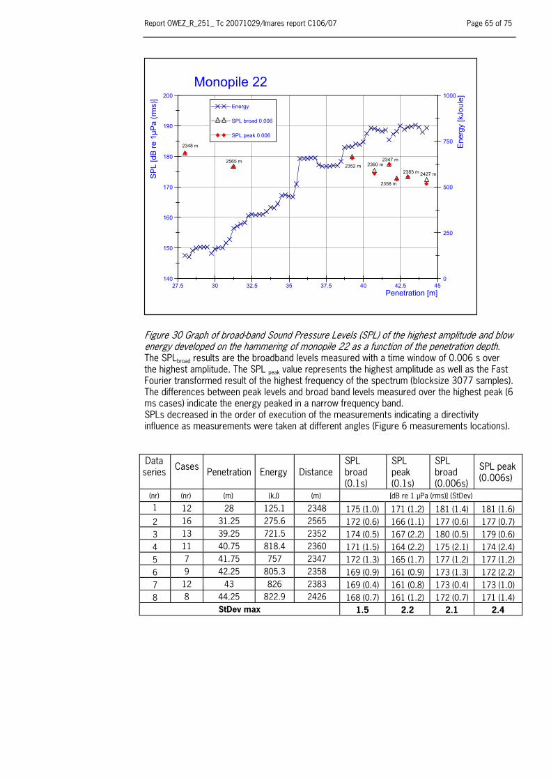
Report OWEZ_R_251_ Tc 20071029/Imares report C106/07 Page 65 of 75
Monopile 22
27.5 30 32.5 35 37.5 40 42.5 45Penetration [m]
140
150
160
170
180
190
200
SPL
[dB
re 1
µPa
(rm
s )]
0
250
500
750
1000
Ene
rgy
[kJo
u le]
Energy
SPL broad 0.006
SPL peak 0.006
2352 m
2358 m
2427 m
2348 m
2565 m 2347 m2360 m
2383 m
Figure 30 Graph of broad-band Sound Pressure Levels (SPL) of the highest amplitude and blow energy developed on the hammering of monopile 22 as a function of the penetration depth. The SPLbroad results are the broadband levels measured with a time window of 0.006 s over the highest amplitude. The SPL peak value represents the highest amplitude as well as the Fast Fourier transformed result of the highest frequency of the spectrum (blocksize 3077 samples). The differences between peak levels and broad band levels measured over the highest peak (6 ms cases) indicate the energy peaked in a narrow frequency band. SPLs decreased in the order of execution of the measurements indicating a directivity influence as measurements were taken at different angles (Figure 6 measurements locations). Data
series
Cases Penetration Energy Distance
SPL broad (0.1s)
SPL peak (0.1s)
SPL broad (0.006s)
SPL peak (0.006s)
(nr) (nr) (m) (kJ) (m) [dB re 1 μPa (rms)] (StDev) 1 12 28 125.1 2348 175 (1.0) 171 (1.2) 181 (1.4) 181 (1.6) 2 16 31.25 275.6 2565 172 (0.6) 166 (1.1) 177 (0.6) 177 (0.7) 3 13 39.25 721.5 2352 174 (0.5) 167 (2.2) 180 (0.5) 179 (0.6) 4 11 40.75 818.4 2360 171 (1.5) 164 (2.2) 175 (2.1) 174 (2.4) 5 7 41.75 757 2347 172 (1.3) 165 (1.7) 177 (1.2) 177 (1.2) 6 9 42.25 805.3 2358 169 (0.9) 161 (0.9) 173 (1.3) 172 (2.2) 7 12 43 826 2383 169 (0.4) 161 (0.8) 173 (0.4) 173 (1.0) 8 8 44.25 822.9 2426 168 (0.7) 161 (1.2) 172 (0.7) 171 (1.4)
StDev max 1.5 2.2 2.1 2.4

Page 66 of 75 Report OWEZ_R_251_ Tc 20071029/Imares report C106/07
2000 2250 2500 2750 3000Distance [m]
140
150
160
170
180
190
200
SPL
[dB
re 1
µPa
Vrm
s ]
SPL broad 0.006s
SPL peak 0.006s
Monopile 22
2
1
3
45
6 7 8
Figure 31 Graph with broad-band Sound Pressure Levels (SPL) as a function of the hydrophone distance from the location of monopile 22. The SPLbroad results are the broadband levels measured with a time window of 0.006 s over the highest amplitude. The SPL peak value represents the highest amplitude as well as the Fast Fourier transformed result of the highest frequency of the spectrum (blocksize 3077 samples). The differences between peak levels and broad band levels measured over the highest peak (6 ms cases) indicate the energy peaked in a narrow frequency band. The positions of data series 4, 6, 7, and 8 were in close range and so were the measured SPLs, the position had a higher outcome, which could also be related to higher depth. (Figure 6). Data
series
Cases Penetration Energy Distance
SPL broad (0.1s)
SPL peak (0.1s)
SPL broad (0.006s)
SPL peak (0.006s)
(nr) (nr) (m) (kJ) (m) [dB re 1 μPa (rms)] (StDev) 1 12 28 125.1 2348 175 (1.0) 171 (1.2) 181 (1.4) 181 (1.6) 2 16 31.25 275.6 2565 172 (0.6) 166 (1.1) 177 (0.6) 177 (0.7) 3 13 39.25 721.5 2352 174 (0.5) 167 (2.2) 180 (0.5) 179 (0.6) 4 11 40.75 818.4 2360 171 (1.5) 164 (2.2) 175 (2.1) 174 (2.4) 5 7 41.75 757 2347 172 (1.3) 165 (1.7) 177 (1.2) 177 (1.2) 6 9 42.25 805.3 2358 169 (0.9) 161 (0.9) 173 (1.3) 172 (2.2) 7 12 43 826 2383 169 (0.4) 161 (0.8) 173 (0.4) 173 (1.0) 8 8 44.25 822.9 2426 168 (0.7) 161 (1.2) 172 (0.7) 171 (1.4)
StDev max 1.5 2.2 2.1 2.4

Report OWEZ_R_251_ Tc 20071029/Imares report C106/07 Page 67 of 75
Monopile 36
20 25 30 35 40 45Penetration [m]
140
150
160
170
180
190
200
SPL
[dB
r e 1
µPa
(rm
s)]
0
250
500
750
1000
Ene
rgy
[kJo
ule]
Energy
SPL broad 0.006
SPL peak 0.006678 m
508 m
1065 m
2325 m
908 m
Figure 32 Graph of broad-band Sound Pressure Levels (SPL) of the highest amplitude and blow energy developed on the hammering of monopile 36 as a function of the penetration depth. The SPLbroad results are the broadband levels measured with a time window of 0.006 s over the highest amplitude. The SPL peak value represents the highest amplitude as well as the Fast Fourier transformed result of the highest frequency of the spectrum (blocksize 3077 samples). When values of broad band and peak levels are close it indicates that the spectrum peaked in a narrow band, when peak levels are much lower it implicates that energy was also detected in a broader frequency band. The differences between peak levels and broad band levels measured over the highest peak (6 ms cases) indicate the energy peaked in a narrow frequency band. The graph and overview show that the SPLs were mainly proportional to the distance range. Data
series
Cases Penetration Energy Distance
SPL broad (0.1s)
SPL peak (0.1s)
SPL broad (0.006s)
SPL peak (0.006s)
(nr) (nr) (m) (kJ) (m) [dB re 1 μPa (rms)] (StDev) 1 15 23.5 86 678 180 (1.4) 176 (1.4) 187 (1.9) 187 (2.1) 2 6 27 273 508 183 (0.4) 174 (1.2) 191 (0.8) 191 (1.2) 3 7 28.5 465 1065 179 (0.3) 171 (0.4) 186 (0.8) 186 (1.1) 4 7 31.25 459 908 178 (0.1) 171 (0.4) 185 (0.7) 180 (2.1) 5 10 36.75 641 2325 169 (0.7) 162 (1.4) 176 (0.4) 175 (1.2)
StDev max 1.4 1.4 1.8 4.0

Page 68 of 75 Report OWEZ_R_251_ Tc 20071029/Imares report C106/07
1 10 100 1000 10000Distance [m]
150
175
200
225
250
275
SPL
[dB
re 1
µPa
(rm
s)]
SPL broad 0.006
Regress SPL 0.006
SPL broad 0.1
Regress SPL 0.1
Monopile 36
Regression function248.23214795386-21.239476302829log(X)
Regression function236.976599469002-19.9089932966064log(X)
Figure 33 Graph with broad-band Sound Pressure Levels (SPL) as a function of the hydrophone distance from the location of monopile 36 and the calculated regression. The SPLbroad results are the broadband levels measured with a time window of 0.006 s over the highest amplitude. The SPL peak value represents the highest amplitude as well as the Fast Fourier transformed result of the highest frequency of the spectrum (blocksize 3077 samples) with the calculation of the logarithmic regression of both cases resulting in the Source Level value and propagation losses factor as calculated result (SL broad 0.1 s 236.98-19.9log(Distance) and SL broad 0.006 s 248.23-21.2log(Distance). The plotted data involve all processed blow cases per distance sequence with numbers listed in the overview table (FFT nr blows). The regression function matches both time window cases as well as the results were more in line than in other cases. Data
series
Cases Penetration Energy Distance
SPL broad (0.1s)
SPL peak (0.1s)
SPL broad (0.006s)
SPL peak (0.006s)
(nr) (nr) (m) (kJ) (m) [dB re 1 μPa (rms)] (StDev) 1 15 23.5 86 678 180 (1.4) 176 (1.4) 187 (1.9) 187 (2.1) 2 6 27 273 508 183 (0.4) 174 (1.2) 191 (0.8) 191 (1.2) 3 7 28.5 465 1065 179 (0.3) 171 (0.4) 186 (0.8) 186 (1.1) 4 7 31.25 459 908 178 (0.1) 171 (0.4) 185 (0.7) 180 (2.1) 5 10 36.75 641 2325 169 (0.7) 162 (1.4) 176 (0.4) 175 (1.2)
StDev max 1.4 1.4 1.8 4.0

Report OWEZ_R_251_ Tc 20071029/Imares report C106/07 Page 69 of 75
Monopile 34
20 25 30 35 40 45 50Penetration [m]
140
150
160
170
180
190
200
SPL
[dB
r e 1
µPa
(rm
s)]
0
250
500
750
1000
Ene
rgy
[kJo
ule]
Energy
SPL broad 0.006
SPL peak 0.006
2500 m
3607 m
726 m
699 m
1326 m 3658 m
1385 m836 m
683 m
2434 m
978 m
836 m
3760 m
Figure 34 Graph of broad-band Sound Pressure Levels (SPL) of the highest amplitude and blow energy developed on the hammering of monopile 34 as a function of the penetration depth. The SPLbroad results are the broadband levels measured with a time window of 0.006 s over the highest amplitude. The SPL peak value represents the highest amplitude as well as the Fast Fourier transformed result of the highest frequency of the spectrum (blocksize 3077 samples). When values of broad band and peak levels are close it indicates that the spectrum peaked in a narrow band, when peak levels are much lower it implicates that energy was also detected in a broader frequency band. The first two cases (with lowest energy) had a very narrow frequency spectrum. The graph shows that the SPLs were mainly determined by the distance range, although the first series indicate an energy relation as SPLs were 5 dB under the level measured in the second series.
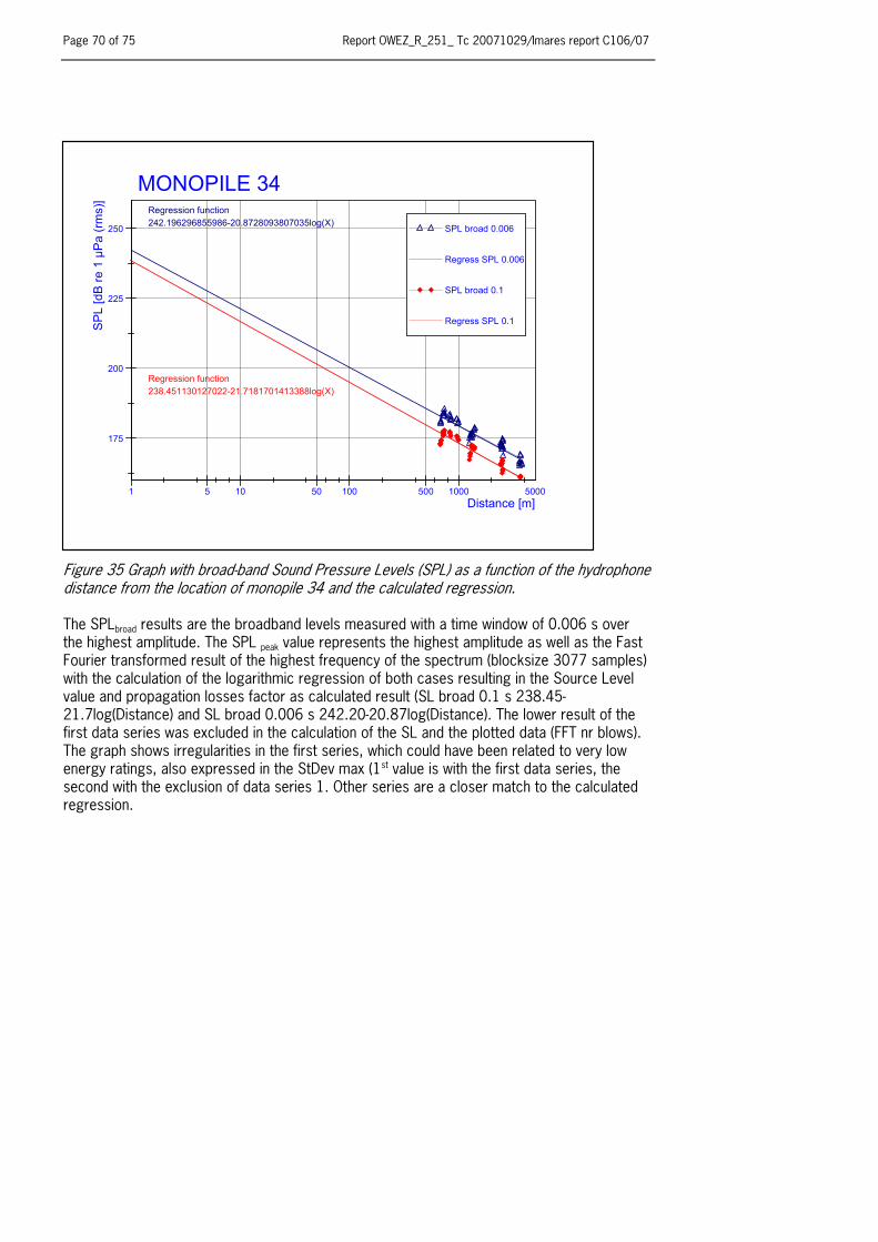
Page 70 of 75 Report OWEZ_R_251_ Tc 20071029/Imares report C106/07
1 5 10 50 100 500 1000 5000Distance [m]
175
200
225
250
SPL
[dB
re 1
µP
a (r
ms)
]
SPL broad 0.006
Regress SPL 0.006
SPL broad 0.1
Regress SPL 0.1
MONOPILE 34
Regression function238.451130127022-21.7181701413388log(X)
Regression function242.196296855986-20.8728093807035log(X)
Figure 35 Graph with broad-band Sound Pressure Levels (SPL) as a function of the hydrophone distance from the location of monopile 34 and the calculated regression. The SPLbroad results are the broadband levels measured with a time window of 0.006 s over the highest amplitude. The SPL peak value represents the highest amplitude as well as the Fast Fourier transformed result of the highest frequency of the spectrum (blocksize 3077 samples) with the calculation of the logarithmic regression of both cases resulting in the Source Level value and propagation losses factor as calculated result (SL broad 0.1 s 238.45-21.7log(Distance) and SL broad 0.006 s 242.20-20.87log(Distance). The lower result of the first data series was excluded in the calculation of the SL and the plotted data (FFT nr blows). The graph shows irregularities in the first series, which could have been related to very low energy ratings, also expressed in the StDev max (1st value is with the first data series, the second with the exclusion of data series 1. Other series are a closer match to the calculated regression.
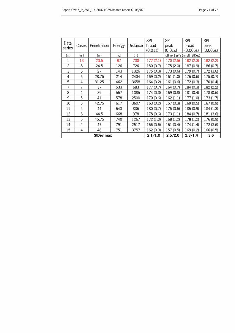
Report OWEZ_R_251_ Tc 20071029/Imares report C106/07 Page 71 of 75
Data series Cases Penetration Energy Distance
SPL broad (0.01s)
SPL peak (0.01s)
SPL broad (0.006s)
SPL peak (0.006s)
(nr) (nr) (nr) (kJ) (m) [dB re 1 μPa (rms)] (StDev)
1 13 23.5 87 700 177 (2.1) 170 (2.5) 182 (2.3) 182 (2.2) 2 8 24.5 126 726 180 (0.7) 175 (2.0) 187 (0.9) 186 (0.7) 3 6 27 143 1326 175 (0.3) 173 (0.6) 179 (0.7) 172 (3.6) 4 6 28.75 214 2434 169 (0.2) 161 (1.0) 176 (0.6) 175 (0.7) 5 4 31.25 462 3658 164 (0.2) 161 (0.6) 172 (0.3) 170 (0.4) 7 7 37 533 683 177 (0.7) 164 (0.7) 184 (0.3) 182 (2.2) 8 4 39 557 1385 174 (0.3) 169 (0.8) 181 (0.4) 178 (0.6) 9 5 41 578 2500 170 (0.6) 162 (1.1) 177 (1.0) 173 (1.7) 10 5 42.75 617 3607 163 (0.2) 157 (0.3) 169 (0.5) 167 (0.9) 11 5 44 643 836 180 (0.7) 175 (0.6) 185 (0.9) 184 (1.3) 12 6 44.5 668 978 178 (0.6) 173 (1.1) 184 (0.7) 181 (3.6) 13 5 45.75 740 1267 172 (1.0) 168 (1.2) 178 (1.2) 176 (0.9) 14 4 47 791 2517 166 (0.6) 161 (0.4) 174 (1.4) 172 (3.6) 15 4 48 751 3757 162 (0.3) 157 (0.5) 169 (0.2) 166 (0.5)
StDev max 2.1/1.0 2.5/2.0 2.3/1.4 3.6

Page 72 of 75 Report OWEZ_R_251_ Tc 20071029/Imares report C106/07
Monopile 10
10 50 100 500 1000 5000 10000Frequency [Hz]
75
100
125
150
175
SPL
[dB
re 1
µPa
(rms )
]
Case 11-2 at 1384 m
Monopile 10
10 50 100 500 1000 5000 10000Frequency [Hz]
75
100
125
150
175
SPL
[dB
re 1
µ Pa
(rms)
]
Case 15-2 at 734 m
Figure 36a Graph of a hammering blow of the monopile 10 series at a distance of 734 m (data series 19, case 2 (2.858s)). a) Peak level 168.6 dB re 1μPa at 180 Hz, with also lower contribution at 70 Hz (-11 dB). The graph expresses a low-frequency cut-off (< 300 Hz) related to shallow water conditions. Figure 36b Frequency spectrum data series 11 case 2 (93.377s) at 1384 m. Sample rate 512 kHz, time window 0.1 s, 51282 samples, dF 10 Hz. Peak level 158.2 dB re 1μPa at 165 and 330 Hz, with also lower contribution at 80 Hz (-6 dB). The graph expresses a low-frequency cut-off (< 300 Hz) related to shallow water conditions.

Report OWEZ_R_251_ Tc 20071029/Imares report C106/07 Page 73 of 75
Monopile 10 FFT seismic wave (8 &15)
10 50 100 500 1000 5000 10000Frequency [Hz]
75
100
125
150
175
SPL
[ dB
re 1
µPa
(rm
s)]
Seismic wave 19
Seismic wave 8
Figure 37 Spectrum analysis of sea-borne diffracted seismic wave captured under a high (data series19) and low (data series 8) energy condition. The curves represent the FFT result of time window of 0.04 s, 20513 samples a frequency resolution ( dF ) of 25 Hz.
Seismic wave monopile 10 data series 8 and 19 Data
Series (nr)
Distance (m)
Time in File (s)
Energy (kJ)
Ampl (Vp/p)
SPL broad [dB re 1 μPa
(rms)]
SPL peak [dB re 1 μPa
(rms)]
Freq peak (Hz)
8 882 126.57
219 0.023 157.23 157.61 125
19 734 2.815 799 0.060 165.49 163.47 125/150
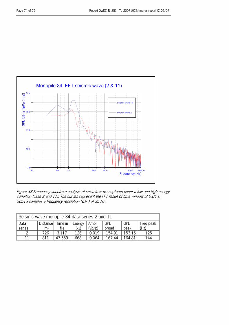
Page 74 of 75 Report OWEZ_R_251_ Tc 20071029/Imares report C106/07
Monopile 34 FFT seismic wave (2 & 11)
10 50 100 500 1000 5000 10000Frequency [Hz]
75
100
125
150
175
SPL
[dB
re 1
µPa
(rm
s)]
Seismic wave 11
Seismic wave 2
Figure 38 Frequency spectrum analysis of seismic wave captured under a low and high energy condition (case 2 and 11). The curves represent the FFT result of time window of 0.04 s, 20513 samples a frequency resolution ( dF ) of 25 Hz. Seismic wave monopile 34 data series 2 and 11 Data series
Distance (m)
Time in file
Energy (kJ)
Ampl (Vp/p)
SPL broad
SPL peak
Freq peak (Hz)
2 726 3.117 126 0.019 154.91 153.15 125 11 811 47.559 668 0.064 167.44 164.81 144

Report OWEZ_R_251_ Tc 20071029/Imares report C106/07 Page 75 of 75
Signature: __________________________ Date: 29-10-2007