report of the sprfmo task group on fishing … · 11. anibal aliaga fishing ompany pesquera...
TRANSCRIPT

REPORT OF THE SPRFMO TASK GROUP ON “FISHING VESSELS AS SCIENTIFIC PLATFORMS”, 2014-2015
INTRODUCTION
During the 2nd SPRFMO Scientific Committee Meeting held in Honolulu, a recommendation was given to create a task group on “Fishing vessels as scientific platform”, with special reference on the use of acoustic data collected aboard fishinf vessels during their fishing trips (SC-02-2014). We cite here the conclusions of the SC report of the 2nd meeting: The SC was requested to establish a Task Group on the Standardization of Acoustic Data from commercial fishing vessels with the following objectives: Establish common protocols (settings of the instruments and calibration procedures; definition of indicators; etc.) Develop collaborative approaches for providing contributions to an ecosystem approach to stock assessment and the provision of ecological and fishing information to SPRFMO Develop a “methodological package” to allow potential users to process their own data under an agreed international format.
The Task Group was proposed for three years under the chairmanship of François Gerlotto (IREA). Participation would be open to all interested Members, CNCPs and Observers. Specialists in acoustics would also be encouraged to join. The working programme of the Task Group would follow the recommendations of the workshop on “Fishing vessels as scientific platforms The terms of reference for the task group activities in 2014-2015 were:
The Task Group will set up an annual workshop and work intersessionally through remote communication means. For the first year (2015), it was recommended that the Task Group work on the development of a protocol for vessel calibration. The Task Group will report to the SPRFMO Scientific Committee and work in collaboration with the ICES WGFAST to avoid any duplication and to ensure the scientific quality of its work.
1. REPORT OF INTERSESSIONAL ACTIVITIES
Two different activities were performed during the intersession: preparation of the workshop on calibration procedure and participation in different scientific event where the theme of “fishing vessels as scientific platforms” was presented and discussed. Contacts with the international community allowed to suggest the creation of international working groups and events during the year 2016, especially inside the ICES /WGFAST activities.. Intersessional activities. They were done by correspondence and consisted in (1) gathering written material on calibration procedure, (2) performing experimental calibrations aboard fishing vessel (SNP – Universidad Villareal, Peru). A list of documents is given in annex. Activities during the COP21, Lima, Dec. 2014:
A series of communications were prepared and presented during a “side event” organized by the SNP on the theme of “Fishing Vessels as Observers of the Oceans”
- Bernales et al. (SNP)

- Gerlotto et al. (IREA)
Elaboration of a common agreement between fisheries organizations of Peru, Chile, Ecuador (SNP). A common document was written and signed by fisheries organizations of Chiule, PEru and Ecuador (annex)igned by SNP, (chilenos y ecuadorianos?)
Presentations of papers to the 6th IcES International Symposium on Marine Ecosystem Acoustics, Nantes, June 2015 - Bernales et al., 2015 (SNP) - Gerlotto et al., 2015 (IREA) - Joo et al., 2015 (IMARPE) Presentation of the Peruvian System of F/V data management, PFA International Workshop , Amsterdam, June 2015 - Bernales and Gerlotto, 2015. Proposal for the organisation of a ICES study Group on fishing vessels as Scientific Platforms. Around 20 manuscripts were submitted, from which a peer review (still in course) under the chairmanship of Dr Gary Melvin (DFO, Canada) is likely to select around 10-12 for publication in the special issue.
2. REPORT OF THE 1st WORKSHOP OF THE SPRFMO TASK GROUP ON “FISHING VESSELS AS SCIENTIFIC PLATFORMS”
The workshop of the Task group was held in Lima, 8th - 11th September, 2015. It was organized by the National Fisheries Society of Peru (SNP) and the Institute of Aquatic resources (IREA) with the support of TNC, WWF, PRODUCE (etc) The workshop was organized in two different parts:
- An open session where conferences were given by invited experts (1 day) - A restricted session where the research of the workshop was performed (3 days). At the
end of this session, recommendations and conclusions were collated and presented in this report.
Following the terms of reference, three themes were considered during the workshop:
1. Calibration procedure for acoustic devices aboard fishing vessels; 2. Establishment of a standardized procedure for “between-calibration” analysis of the
acoustic data collected aboard fishing vessels; 3. Definition of the priorities for the following activities of the Task Group.
Theme 1 being the most important, 2 full days were dedicated to the development of the calibration protocol. Themes 2 and 3 were considered during the third day, and the conclusions were presented during the plenary open session. The output of the workshop is a draft document describing the calibration procedures and protocols adapted to fishing vessels that will be submitted and discussed during the 3rd SPRFMO Scientific Committee meeting in 2015.

LIST OF PARTICIPANTS – ACOUSTIC SPRFMO TASK GROUP WORKSHOP
1. Francois Gerlotto (Task group Coordinator) France 2. Ulises Munaylla National Fishery Society- SNP 3. Adam Dunford New Zealand 4. Gary Melvin Canada 5. Dirk Burggraaf IMARES - Holland 6. Jorge Castillo IFOP – Chile 7. Carolina Lang IFOP - Chile 8. Rocío Joo Mar. Res. Institute of Peru- IMARPE 9. Mariano Gutiérrez National University “Federico
Villarreal”-UNFV 10. Salvador Peraltilla Fishing Company- TASA 11. Anibal Aliaga Fishing Company “Pesquera
Diamante” 12. Cynthia Vasquez SNP-UNFV 13. Gloria Meneses SNP 14. Jose Luis Rojas Fishing Company- AUSTRAL 15. Cristian Vasquez Fishing Company -TASA 16. Carlos Valdez TASA-UNFV 17. Alex Espinoza Fishing Company “Pesquera
Diamante” 18. Marisol Llaguento Ministry of Production –PRODUCE
CALIBRATION PROCEDURE AND PROTOCOLE Calibration can be defined as: a comparison between measurements – one of known magnitude
or corrected, or scaled with one reference device, and another measurement made in as similar
way as possible with a second device. Acoustic instrument calibration is fundamental in order to
quantitatively use the data for estimating aquatic resource abundance. Regular calibrations also
allow instrument performance to be monitored and to detect changes due to the environment
or component dynamics, degradation, or failure. Since the work of Foote et al. (1987), acoustic
calibration of fisheries echosounders is usually performed by comparing the results obtained on
a reference target to its theoretical value.
The first activity of the task group was to develop a standard protocol for calibrating commonly
used acoustic devices aboard fishing vessels, so that scientific information can be extracted from
their echograms. The protocol is mostly designed for fishing vessels operating the SPRFMO area
that will be used for monitoring of fish stocks in the South Pacific Ocean. However calibration is
a universal operation and this protocol should be applicable any time acoustic data are used to
monitor a fish stock. In the case of SPRFMO, fisheries are persecuted by industrial ships using
mostly Simrad ES or ES70 split beam echosounders. The calibration protocols focus mostly on
the characteristics of these systems. It is given in annex.
There was a general consensus that no major difficulties exist for the calibration fishing vessels
provided they are using SIMRAD ES split-beam systems, which is the case for most of the fishing
vessels in the SPRFMO region. The quality of acoustic data collected aboard fishing vessels, once

calibrated, is therefore acknowledged by the scientific community and comparable to that of
research vessels.
The group recommended that the calibration of the fishing vessels follow the general procedures developed by ICES (ICES Cooperative Research Report nº 326, 2015) using specific copper or tungsten sphere as a reference target. It is further recommended that a complete calibration of the echosounder be performed at least once a year, preferably before the beginning of the fishing season.
“BETWEEN-CALIBRATION” ANALYSIS OF THE ECHOSOUNDER CHARACTERISTICS
OBJECTIVES / RATIONALE
Calibration is recommended to be performed on a yearly base. Modern echosounder systems
are relatively stable in their performances and are unlikely to drift from the standard values
Annual calibration is already an expected effort required from the fishing companies, and data
analysis with calibration at this rhythm looks realistic.
Nevertheless annual calibration presents a drawback: when a failure event occur (e.g. loss of a
quadrant of the split-beam transducer) all the data collected after the last calibration must be
rejected, which could represent up to one year of data. In order to reduce this period and to
insure that the data are of good quality, a “between-calibration” analysis of the behaviour of
the system must be performed in order to:
Evaluate the stability of the echo sounder characteristics and the possible existence of
troubles in a given instrument between calibrations
Perform a quality control of the data collected during fishing trips.
This requires that tools and methods to be used by the fishing companies be developed.
METHODS
a. Choice of methods
A list of potential Between-Calibration-Analysis (BCA) methods to monitor the performance of
the acoustic systems is provided below.
Bottom reflection
Impedance testing
Monitor beam pattern with fish targets
Fish in all-beam quadrants
Movements of targets
Ringdown zone
After analysis, it appeared that only 2 of these methods present the conditions required for use
aboard fishing vessels: Bottom reflection and ringdown zone. These two methods are briefly

presented here. The other methods either are requiring particular scientific equipment or
complex scientific methodology that cannot be easily implemented aboard fishing vessels.
Ringdown zone
Bottom reflection. One approach to evaluate the performance and to identify
issues, if they arise, for a fishing echo-sounder is to monitor the reflective
properties of a constant section of bottom over time. Fishing vessels often tie-
up at a specific location of a wharf for unloading and/or mooring. Assuming
the small section of bottom under the vessel is relatively consistent
acoustically then recording the echo-sounder data while it is stationary and in
the almost exact same place should provide a mechanism for comparing
bottom backscatter between trips. While there will be some variability due to
slight differences in positioning of the vessel and bottom variability, it should
be possible to establish a range of acceptable mean backscatter values of the
bottom. If major difference are observed then further investigation of the
system outputs should be undertaken to ensure that the calibration remains
valid, and if not when the problem began during the previous trip.
b. Informations to be collected.
The two methods utilize the same data but require examination of different sections of the
echogram : for ringdown zone the necessary data are near-transducer echoes; for bottom
reflection the data are the bottom echoes. These two sets of data are included in raw output of
standard echograms that includes the bottom. Therefore, the only requirement is that the
echosounder be set to record while in port Moreover in the case of ringdown zone, the data are
collected continuously when the echosounder is on. For bottom reflection, one simple action,
when the fishing vessel is mooring in the same place between fishing trips, is to set the
echosounder on one hour before or after the trip once the ship moored. This has the great
advantage that nothing is different from the standard recording.
These two sets of data are used for two different analyses: succinctly they are used to determine
if (bottom reflection has changed) and when (ringdown zone) a problem occurred.
- Bottom reflection. It is used to make a quick check of the acoustic properties of the
system at the beginning and at the end of a trip. A large difference in the bottom
reflectivity would lead to conclusion that the system suffered a problem. In this case
either the whole data set of the trip is discarded (e.g. for short trips of a few days) or
the second method is used to define when this event occurred.
- Ringdown zone. It is used to go back in the pass and determine when the acoustic
properties of the system changed. As the data required are continuously collected, it
becomes possible to determine the precise moment of the event, therefore only the
data collected after the problem would be lost. This is particularly important during long
fishing trips (e.g. several weeks) in order to avoid discarding large amounts of
information.

c. Processing the information
- Data are processed by analyzing the echogram for significant inconsistency in the
target region of the echogram using dedicated softwares (already existing or to be
written). This is done by extracting the echo amplitude. Information on the bottom
reflection should be processed at the beginning/end of each trip, while that on
ringdowm zone should only be processed when the former showed that an event
occurred. In the future automated detection methods will be available to
continuously monitor the system performance.
- What to do with the results?
i. Use for data acceptance checking
ii. Short trips: accept/reject the whole trip
iii. Long trips: use the “when” function to select the acceptable data
iv. Use to determine if a new full calibration is needed
RECOMMENDATIONS
The works of the task group has shown that there are solution for evaluating the overall quality
of the data, selecting the acceptable sections and rejecting the others. It is not the objective of
the task group to develop a complete protocol for these methods, as they are still (in the case
of ringdown zone) under development and validation. But it is clear that these methods will be
available for routine application within the coming years, because of the growing interest of the
international community (scientists as well as fishers) in using acoustic data from fishing vessels.
The action of the task group now is to alert the ICES WGFAST which should recommend its sub-
group on fishing vessels as scientific platform to develop research for these methods.
It is recommended to begin to record bottom echoes, in order to collect data for defining
protocols and evaluating the consistency of these echoes for answering the question of BCA.
“BETWEEN-VESSEL INTERCALIBRATION”
The question of intercalibration the fishing vessels arose and a protocol has been written that is
included in the calibration protocol as an annex.
It is important to understand why intercalibration was recommended.
Intercalibration consists in comparing the data collected by two or more vessels sailing close to
each other (i.e. assuming that they record the same or similar echoes) over a given distance.
Intercalibration IS NOT a way to avoid calibrating a ship. It has several specific reasons.
- Establishing the signature of each vessel. The data collected by a given vessel
are affected by 3 particularities of this ship: acoustic performance of the
instruments (this should be corrected by calibration); noise of the vessel, which
affects the signal-to-noise ratio and therefore the acoustic values at high or low
densities; the “frightening signature” of the vessels, which describes the way
fish avoid this particular vessel, and is usually due to particular characteristics

of the sound emitted by the ship. These three factors are specific to each vessel,
and comparing their data would normally require that they are all inter-
calibrated. In practice this is impossible and usually not necessary.
- Including in the data from a vessel which has an acoustic system is different
from the others (e.g. sounder of a different origin).
- Including data of an uncalibrated vessel which are of particular interest. For
instance, if the ship is the only one which has been in an interesting area, etc.
The intercalibration protocol is presented in annex.
3. RECOMMENDATIONS FOR 2015-2016
A list of activities that the use of acoustic data from fishing vessels would require has been
established by the task group. They are the following:
- Technical and methodological research. It consists in improving the techniques and
methods applicable to fishing vessels, e.g. better collection and processing of data,
simpler protocol for calibration, choice of ancillary data to be added to the data
collection, etc. The improvement of the calibration protocol and the production of a final
version should also be part of the next activities of the task group.
- Definition of data format and data bases. Once the data correctly collected and
calibrated, the logical next step is to design a common format for data base elaboration,
in order to make comparable all the different data collections. This presents two major
parts: (1) list the data to be collected and input in a common base, which requires to
select the metrics and list the indicators that are needed in any research on the fish
populations (see below); (2) elaborate a structure for the data base.
- Identification of fish species and length. This point represents a priority question from
the fishing companies. Some progresses have been made in this field by those working
with multifrequency and broadband echo sounders and it is likely that dramatic
improvements be achieved in the forthcoming years. Nevertheless it is still early in the
research and no method for absolute identification (with 100 % of probability) is to be
expected before a couple of years. Given the importance of this subject the task group
recommends that this question should be transmitted to the ICES WGFAST for
consideration.
- Statistical methods for acoustic samplings by fishing vessels. Fishing vessels use a
highly adaptive survey method, which makes the use of conventional statistics
impossible. Finding adapted statistical methods would greatly improve the use of such
data, and it seems important to develop common research with geo-statisticians on this
topic.
- The use of acoustic data in stock and ecosystem models. So far acoustics is mostly
providing biomass estimates obtained from acoustic surveys. Most of the information
obtained by such devices is not used. Defining the metrics and indicators that could be
used by the models should be of great interest and certainly represents a priority. The
JM fisheries in the SPRFMO area may contain rather important data that could be used
for defining such metrics and indicators.

- Comparing acoustic surveys and fishers observations. This represents an important
point, with several objectives: comparing the data from both sources of information;
comparing methods for abundance estimates; evaluating in what way synthesizing the
two data sets would allow to improve the biomass estimates; etc.

SPRFMO Task Group on “Fishing vessels as Scientific Platforms
Task Group Report, September, 2015
CALIBRATION PROTOCOL FOR FISHING VESSELS
Participants:
Francois Gerlotto (Task Group coordinator) France Ulises Munaylla National Fishery Society- SNP Adam Dunford New Zealand Gary Melvin Canada Dirk Burggraaf IMARES - Holland Jorge Castillo IFOP – Chile Carolina Lang IFOP - Chile Rocío Joo Mar. Res. Institute of Peru- IMARPE Mariano Gutiérrez National University “Federico
Villarreal”-UNFV Salvador Peraltilla Fishing Company- TASA Anibal Aliaga Fishing Company “Pesquera
Diamante” Cynthia Vasquez SNP-UNFV Gloria Meneses SNP Jose Luis Rojas Fishing Company- AUSTRAL Cristian Vasquez Fishing Company -TASA Carlos Valdez TASA-UNFV Alex Espinoza Fishing Company “Pesquera
Diamante” Marisol Llaguento Ministry of Production PRODUCE
DRAFT

1 INTRODUCTION
The South Pacific Region Fisheries Management Organization (SPRFMO) created in 2014 a
dedicated Task Group on the theme of “fishing vessels as scientific platforms”. The first activity
of the task group was to design a standard protocol for calibrating acoustic devices aboard
fishing vessels, in order to be able to extract scientific information from their echograms.
Therefore this protocol is mostly designed for the SPRFMO area, for monitoring of fish stocks in
the South Pacific Ocean. Nevertheless calibration is a universal operation and should be applied
any time acoustic data are used to monitor a stock. In the case of SPRFMO, fisheries are operated
by industrial ships using mostly Simrad ES split beam echosounders. Therefore this protocol will
focus mostly on the characteristics of these echosounding systems..
The main target for calibration will be SIMRAD ES60 and ES70 split beam echosounders which
are the ones most commonly used by SPRFMO fisheries. Because these systems have identical
hardware but different operating software, calibrations with either of the operating software
versions can be considered identical within the measurement uncertainly (O’Drisocll and Nelson,
2010). The differences in software will be noted in the protocol where applicable.. The
frequencies most commonly used in the SPRFMO area are 120 kHz and 38 kHz, however much
of this document is not frequency-specific. Where specific calibration procedures are required
for other frequencies, this will be specified in the document. Calibration of other echosounders
such as Furuno etc. is not considered in this document, although these echosounders should be
calibrated as well. The general principles are similar, but the methodology being rather different,
and considering that they are not as common, we do not consider them in this document.
Post-processing of data from echosounders requires dedicated software. One common software
for analysis is ECHOVIEW and it is applicable to data from both ES60 and ES70. he section on
post-processing in of this protocol describes the required analysis methods using this particular
piece of software. For data collection, this protocol follows the procedure defined by ICES as
published in the CRR326. It represents a synthesis of the protocols designed in the different
member countries of SPRFMO who participated in this workshop (Chile, EU (Holland and
France), New Zealand and Peru) and those of countries outside the SPRFMO area (Canada,
Argentina). The major contributions for this work come from New Zealand and Peru, and the
task group is particularly grateful to Adam Dunford, Salvador Peraltilla, Mariano Gutierrez and
Cynthia Vasquez for their contributions.
2 OBJECTIVES
Calibration can be defined as: a comparison between measurements – one of known magnitude or
correctness made or set with one device and another measurement made in as similar way as
possible with a second device. In the case of acoustic calibration, since the works from Foote et
al. (1987), calibration is performed by comparing the backscattered power from on a reference
target to its theoretical value (figure 1). Acoustic instrument calibration is fundamental in order
to allow the quantitative use of the data for estimating aquatic resource abundance. Regular
calibrations also allow instrument performance to be monitored to detect changes due to the
environment or component dynamics, degradation, or failure.

Figure 1. Calibration of digital sounder: drawing of the calibration procedure and methodology
(from ICES CRR326)
The main objective of this work is therefore to generate a technical protocol to describe the
required equipment, processes and methods for calibration of echosounders installed on the
hulls of fishing vessels.
Intercalibration between fishing vessels equipped with echosounders, either calibrated or not,
will also be considered in this report, but its objectives, methodology and results being quite
different from a calibration, this will be presented in an appendix.
3 GENERAL REQUIREMENTS
Time:
Once the ship is in place, under ideal conditions, the time required for calibration of an
echosounder using a reference target sphere is about 8 hours.
Environmental conditions:
Calibration should be done in a place where the depth is more than 20 meters; characteristics
of the sea water at the calibration site (general vertical profile and values at transducer and
sphere depth) should be measured to be input in the calibration equations.
Sea conditions:

No waves, no tides, no current, no wind, no traffic, the water is well mixed and relatively void of
biological scattererss.
Site selection.
As much as possible, calibration experiments should be conducted over the range of
environmental conditions encountered during the survey measurements. Calibrations should be
performed in areas where the water is well mixed and relatively void of biological scatterers.
The experiment should be scheduled for slack tide. The water depth should be sufficient to place
the sphere in the far-field of the transducers accounting for tides (i.e. deeper than 15 m,
preferably 20-30 m).
Depending on the location, traffic, wind, swell, and current, the sphere calibration may be
conducted while the vessel drifts in the open ocean or anchored from one or more points. If the
wind speed is < ~15 knots and the swell is < ~2m, drifting may be most convenient. More often,
however, anchoring in a sheltered bay or fjord is a better option. If the vessel is drifting or
anchored from a single point, usually the bow, vessel, and tethered sphere tend to move in
unison with any current. However, if the wind and current are from different directions, the
vessel may be anchored from multiple points, e.g. the bow and stern, to keep it from swinging.
Personnal:
There are several activities to be done that require several operators: positioning of the sphere,
measurements of oceanographic conditions, survey echosounder operation, setup of the
calibration equipment, possibly a diver, etc. The minimum number of personnel is about 4.
Equipment:
A reference calibration sphere (see below)
Equipment for cleaning the transducer.
3 fishing rods, nylon yarn (0.6 mm diameter) and weight (see below)
A CTD, which is used to measure the physical characteristics of the sea (temperature,
salinity).
Printed version of the calibration protocol
Relevant information for the vessel to be calibrated including fishing pole positions
(Optional) Values from previous calibrations
Calibration kit (see list in Appendix)
Calibration fishing poles
CTD logger
Spare batteries for CTD logger
USB drive for data
USB pen drive (as backup storage)
Mouse + Keyboard
(Optional) Laptop with CTD software and post processing software installed
Optional) Camera (for photographing setup)

The Calibration spheres
Foote et al. (1987) defined a method for calibration of echo sounders using a reference sphere
of precisely known acoustic characteristics, with a diameter adapted to a single frequency. This
is acknowledged as the reference method (MacLennan & Simmonds, 2005), The TS of these
reference spheres have been calculated or measured. Companies like Kongsberg and Biosonics
provide such spheres that are generally made of copper (Cu) or tungsten carbide (WC).
NOTE. Any damage on these sphere is likely to change their acoustic characteristics. Therefore
it is strongly recommended to treat them with caution.
Table 1 shows the different target strengths (TS for its acronym in English), and the
corresponding diameters for each frequency, "Cu" denotes copper and "WC" is denoted
tungsten carbide.
Table 2.3. Approximate theoretical target strength, TS (dB re 1 m2 at r0 = 1 m), of
common calibration spheres with various diameters (mm), made from tungsten carbide
with 6% cobalt (WC) , copper (Cu), at 𝒕𝒘 = 𝟏𝟑. 𝟓 , 𝒔𝒘 = 𝟑𝟑. 𝟑 𝐩𝐬𝐮 , 𝒑𝒘 = 𝟐𝟓. 𝟎 𝐝𝐛𝐚𝐫, 𝒄𝒘 = 𝟏𝟓𝟎𝟎
𝐦 ∙ 𝐬−𝟏, and 𝝆𝒘 = 𝟏𝟎𝟐𝟓.𝟎 𝐤𝐠 ∙ 𝐦−𝟑. Green indicates there are no nulls within or near the signal
bandwidth (𝒃𝒇 ≈ 𝒇 ± 𝟎. (𝟏⁄𝝉), where 𝒇 is frequency (Hz) and 𝝉 is pulse duration (𝐬). Yellow
indicates a null close to the 𝒃𝒇, and red indicates a null within the 𝒃𝒇.
Material
Diameter (mm) f ∙ 10-3 (Hz)
𝝉 ∙ 10-6 (s) 64 128 256 512 1024 2 048 4 096 8 192
WC 20.0 18 38 –49.7 -49.7 –49.7 -49.7 –49.7 70 -47.6 –47.8 -47.8 –47.8 -47.8 120 –45.8 -45.6 –45.6 -45.5 –45.5 200 -45.2 –45.1 -45.0 –45.0 –45.0 333
WC 21.0 18 38 –49.8 –49.9 –49.9 –49.9 –49.9 70 –47.3 –47.4 –47.5 –47.5 –47.5 120 –46.0 –46.2 –46.3 –46.3 –46.3 200 –45.5 –45.5 –45.5 333 –44.4 –44.4 –44.4 –44.4
WC 22.0 18 38 –49.6 –49.6 –49.7 –49.7 –49.7 70 –46.1 –46.2 –46.3 –46.3 46.3 120 –45.9 –46.2 –46.3 –46.4 –46.4 200 333 –44.1 –44.1 –44.1 –44.1 –44.1
WC 38.1 18 –42.6 –42.6 –42.6 –42.6 –42.6 38 –42.2 –42.4 –42.4 –42.4 –42.4 70 –41.3 –41.4 –41.4 –41.4 120 –39.5 –39.5 200 –39.1 –39.1 –39.1 333
Cu 60.0 18 –35.4 –35.4 –35.4 –35.4 –35.4
38 –33.7 –33.6 –33.5 33.5 33.5 70

Salinity
affects strongly the TS characteristics. A calibration in waters with significant different salinities
from the average sea water should take this point into consideration (table 2)
Table 1: The variation of target strength betweem fresh- and sea-water for different frequencies for a
38.1 mm diameter WC sphere.
Frequency
(kHz)
Fresh water TS
(dB)
Seawater TS
(dB)
38 –42.1 –42.4
70 –40.6 –41.0
120 –39.8 –39.5
Source: Simmonds, J. & MacLennan, D. (1992).
4 METHODS
4.1. Calibration
The Vessels must have connections with shielded cables, in order to reduce noise in the
echograms.
To Obtain adequate advantage of these systems they must be calibrated at least once a year.
For this, each company must have at least one professional analyst is also able to interact with
other professionals to correctly analyse the recorded calibration and monitoring data.
Echo sounders are calibrated according to the procedure outlined by Foote et al 1987 and
Simmonds et al. (1992) and as updated in ICES CRR326.
The environment conditions must be measured before performing any calibration
measurement in order to allow the use of the equation of MacKenzie (1981) that evaluates
empirically the propagation speed of sound (c) (see Appendix)
Where the average temperature (° C) and salinity (psu) between the transducer and sphere has
been measured, the corresponding absorption coefficient (α) can be determined from the
equations listed in the Appendix (same one as sound speed equations) and illustrated in Figure
2 below.
120 200 333

Figure 2: Absorption coefficient (from doc. EK60 according to Francois & Garrison, JASA diciembre 1982.)
4.2. Noise measurement
TNoise is unwanted signal and can dramatically reduce the quality of the calibration: the lowest
background noise is the best. Noise comes from either acoustic sources: environmental (ocean
waves, winds, currents, biological noise), or mechanical (engine, propeller, vibration, cavitation)
and noise from non-acoustic sources such as: electronic noise, thermal noise, etc.) These noise
signal sources are independent of those due to the transmission of the echo sounder that are
observable in the echogram (see Annex 3, Figure 5). In the particular case of calibration (vessel
at anchor or drifting), the decision to perform it or not depending on the noise observed on the
echogram would be done from the experience of the operator.
NOTE. This is different from the noise measurements made during surveys, which are performed
for other purposes and will not be considered in the “calibration” part of this document.
4.3. Interferences
Interference is a particular source of noise caused by reception of sound transmitted on a similar
frequency by another echounder or sonar. Interference affects the accuracy of the measured
acoustic echo power as it is no longer possible to be certain that all the reflected sound was due
to the echosounder being calibrated (Appendix 3, Figure 6). Here too it is essential to be sure
that there is no interference before to perform a calibration.
4.4. Intercalibration
The procedure for intercalibration of vessels is given in the Appendix, as it has different
objectives than a standard reference sphere calibration. Indeed intercalibration is a comparison
in the capacities of different vessels to give the same result when observing the same place. This
helps evaluating the accuracy of the results of a vessel.

Intercalibration is not an alternative to calibration for one of the two ships involved in the
intercalibration experiment: both must be calibrated. But in some cases calibration of one ship
may be impossible (e.g. a non scientific echo sounder aboard); in this case intercalibration can
be a way to get relative information on the acoustic sampling characteristics of this vessel.
4.5. Calibration procedure
The basic procedure is to get the sphere in the main lobe of the transducer beam and then
record some data with the sphere on-axis (to measure the Sa correction) and some with the
sphere moving around the main lobe (to measure beam parameters).
The following protocol presents procedures for theES60 which is the most common
echosounder of the fishing fleet. Although the ES70 has identical hardware, slight differences
in the software require different operations that will be presented when necessary. It is
important to note that the critical software difference between the ES60 and ES70 is that the
ES70 can automatically vary pulse lengths if this option is selected. For scientific use this
option must not be selected.
4.6. Practical operations.
Setup and deploy the CTD Logger, to log at the fastest rate, and for the duration of the
calibration.
Record the station and system information, e.g. date, position, software versions etc in
the calibration log sheet.
Check and record the echosounder settings.
For the ES60, right-click on the frequency (e.g. 38 kHz) indicator in the top left
of the main window (figure 1), to bring up the ‘Transceiver Settings’ dialog box
(figure 2). For 38 kHz, the transmit power should be set to less than or equal
to 2500W and 250 W for 120 kHz (Korneliussen et al., 2008); any higher value
has the potential to cause cavitation and render the calibration worthless. For
practical reasons we recommend 2000 W and 250 W for the two frequencies,
respectively. Click the ‘Advanced’ button, and record the system gain,
bandwidth, sampling interval and pulse length (figure 3).
For the ES70, in the Operation menu, click Normal to open dialog box. Make
sure Mode = Active, and set Power and Pulse Length to the required values.
The example below is for 2000W and 1.024 ms. The transmit power is
extremely important and should be set to less than or equal to 2500W for 38
hHz or ≤ 250 W for 120 kHz (Korneliussen et al., 2008); any higher value has
the potential to cause cavitation and render the calibration worthless. For
practical reasons we recommend 2000 W and 250 W for the two frequencies,
respectively., It is also extremely important to ensure the automatic pulse
length is NOT selected

To set the ping rate to maximum for the ES70, in Operation menu, click ping
mode and select Maximum. The example below is to set a fixed ping interval of
2s. (figure 1)
Figure 1
For the most commonly used 120 kHz (ES120-7C) or 38 kHz (ES38B) transducer
the values should be the same as in the calibration log sheet. If the transducer
is not one of these models, record the correct values (figure 2) .
Figure 2
Figure 3
2000 ms

Set up the echo sounder. The echogram TVG should be set to ‘Fish’ (40 log TVG).
For the ES60, this setting is in the dialog box obtained by right-clicking the
mouse when it is in the top echogram part of the ES window (shaded red area
in figure 4).
Right-click on the colour bar (top right of main window – figure 5), and set the
echogram ‘fish’ colour scheme threshold as low as it will go (-100). This allows the
sphere to be visible even if it is in a sidelobe. Once it is in the main lobe this setting can
be changed.
Figure 5

For the ES60, the minimum dB value on the x-axis of the splitbeam target strength
histogram display is determined by the echogram colour scheme. The maximum value
is about 30 dB greater than this. Any targets that have target strengths greater or
lower than this range are put into the upper or lower histogram bins respectively.
Hence it is important that the histogram dB range adequately covers the expected
target strength of the calibration sphere. Setting the echogram colour scheme
threshold to -60dB is suitable. For the EK60 the minimum dB value is set in the ‘single
target detection’ dialog box obtained by right-clicking in the ‘TS’ part of the window.
Single targets displayed in the splitbeam histogram and position display are taken from
the same depth range as the echogram depth range. Hence to show just the splitbeam
data from the calibration sphere, set the echogram depth range to encompass the
sphere depth (±5 m or so).
Right-click to the right of the upper echogram to get the dialogue box (shaded
red area in figure 6).
Set the range to 5 above the target sphere, and ‘Start RelativeSurface’
to 10m (figure 7).
Figure 6
(figures for ES60 120 kHz)

Figure 7
Set the bottom detection range to 50m (i.e. greater than the sphere depth).
To call up this dialogue box, right-click on the top of the main window where
the bottom depth is displayed (figure 8).
Figure 8
Set up the calibration poles. The example given here comes from the New Zealand
experience. The protocol should be common to all fisheries, but the list of material to
be used is related to the actual possibilities in each harbor. Using the Penn reels, bolts
and spanner in the calibration kit and the poles and cross bars in the plastic tube.
Attach the poles in the appropriate places using cable ties to hold the cross bar onto
the railing and the rope in the kit to hold the end of the pole down.
If the places to attach the poles cannot be determined by reference to a previous
calibration (e.g. if this is the first time the vessel has been calibrated), the general
procedure is to place the first pole in line with the transducer and the second and third
poles on the opposite side of the ship and equidistant from the line of the transducer.
Obtain a tripod of lines with a calibration sphere and weight hanging below
underneath the transducer. There are two ways of doing this, depending on whether
divers are used to assist in getting the sphere located:
1) Without divers
a) Pass a line under the keel of the vessel, either by throwing a weighted line off
the bow while holding both ends or by using the ship’s boat to pull one end
around (the weighted line is usually quicker, but is not always successful).

b) Take the swivel on the end of the line from the reel which is by itself and
attach it to the rope running under the keel along with one of the misc.
weights from the kit. Pull the rope underneath to the other side of the ship
until the line with the swivel is on the same side as the other two. Remove the
rope and weight from the swivel.
c) Take the 2m loop of nylon from the kit and connect all three swivels together
using the swivel hook on the monofilament loop. Attach one of the 750g
weights with the 3m of spectra attached, by connecting its hook to either the
swivels or the hook on the nylon loop. The weight should hang 3m below the
swivels.
d) At the other end of the nylon loop thread on one of the specific tungsten
carbide or copper calibration spheres by looping its thread through the
monofilament. Do not use a swivel hook to attach the sphere, as this would
interfere with the sphere echo. The sphere should now be approximately 2m
below the swivels and 1m above the 750g weight. NOTE: if a longer pulse
length (e.g 2ms) is used then more distance is needed between the sphere and
weight to prevent overlapping echoes. Measurements must be done on a
sphere which temperature is that of the sea water, which is the case after a
few minutes of immersion.
e) Soap the sphere and nearby knots and lines in a mixture of ¼ detergent and ¾
fresh water.
f) Lift the sphere and weight over the side of the ship, taking care not to touch
the sphere, and lower them into the water. With the sphere just on the
surface pay out equal amounts of line from each of the two reels, sufficient to
reach under the keel and up the other side (30 to 35 m is usually necessary).
Note how much line is paid out. Lengths are marked on the calibration pole.
g) Go back to the side with the single reel and wind in until the sphere appears at
the surface. Now pay out the same amount of line as on the other two reels
and with a bit of luck the sphere will now be suspended below the ship on a
tripod with three equal lengths of line. Some adjustment to the line length
may be necessary if the height of the poles above the water varies.
h) If the sphere is not visible, let out 10 m more of line on all three reels, as the
deeper that the sphere goes, the wider the beam.
i) If there sphere is still not visible move the lines in and out by 5 m in steps of 1
m. Do each line separately, returning to the original position after varying one
line.
2) With divers – ensure all sounders are OFF when divers are in the water

a) Lower the single line, with one of the large weights, to the diver in the water.
b) Diver swims single line to transducer, attaches line to hull and removes weight.
c) Connect the swivels of the two remaining lines together and attach the
monofilament loop, sphere and weight (as above). The weight should hang 3m
below the swivels. Do not use a swivel hook to attach the sphere to the nylon
loop, as this would interfere with the sphere echo. The sphere should now be
approximately 2m below the swivels and 1m above the 750g weight. NOTE: if
a longer pulse length (e.g 2ms) is used then more distance is needed between
the sphere and weight to prevent overlapping echoes.
d) Soap the sphere and nearby knots and lines in a mixture of ¼ detergent and ¾
fresh water.
e) Lower the lines, sphere and weight to the diver in the water who will swim
under the hull and attach on the single line.
f) When the diver signals that the lines are connected, usually by tugging on one
of the lines, wind in all three lines so they are tight against the hull.
g) Slowly pay out lines, in small (~5m) increments to the desired depth. Have the
diver check if the sphere is drifting in a particular direction.
h) Have the diver exit the water and turn on sounder. Hopefully the sphere will
be in the beam. If not, and the diver noted a drift direction, adjust the lines to
compensate.
i) Keep the divers around until the sphere is on axis, and ~10 min of data has
been recorded. (See below for how to do this). After this, hopefully things are
working sufficiently well and the divers can depart.
Once sphere echoes are observable and the sphere has moved towards the centre of
the beam, which will possibly saturate the colour scale, change the echogram threshold
to –60 dB (click on the bar as shown in figure 2 and adjust the scale for ‘Fish’). This
should then give a target strength histogram which covers the –42.4 dB value of the
sphere (at 38 kHz in seawater, for other values see Calibration sphere values) Note down
the time the sphere first appears in the main lobe in the calibration log sheet.
Check that the graph on the top left is set to display the right units.
Right-click the top left graph (shaded red area in figure 9) and set
‘Presentation’ to ‘both’, ‘Scale’ to ‘TS’.

Figure 9
Record calibration data.
ES60: By default, neither the ‘raw’ or ‘output’ data streams are recorded
when recording acoustic data. They need to be turned on from the dialog box
accessible from the ‘File:Store’ menu (figure 10).
Figure 10
ES70: In the Operation menu click on Record, then File Output to bring up the
dialog box. In the Directory field, use Browse to select the folder you have
created for data storage (on the USB hard drive). In the Raw Data field, set the

range to deeper than the maximum bottom depth you want to record to and
set Max file size to 100 MB. Do not check Save raw data box unless you want
to start recording. In the Processed Data field do not check Save EK500.
5
If the ES70 computer crashes for any reason, you will need to reset the data
file-path to point the files at the USB drive (this does occur!).
To record data, in the Operation menu, select On to start recording and Off to
stop recording. The current status will be indicated.

4.7. Post- processing
Triangle-wave error (this paragraph is extracted from ICES CRR326)
(extracted from CRR326)The raw data from ES60 and ES70 echosounders are modulated with a
triangle-wave error sequence (TWES) with a 1-dB peak-to-peak amplitude and a 2720-ping
period (Figure 4.1) (Ryan and Kloser, 2004). The TWES averages to zero over a complete
period, so its contribution to sampling error may be insignificant. However, the TWES may bias
calibration results as much as ±0.5 dB. Therefore, prior to calibrations, the TWES should be
removed from ES60 or ES70 𝑃𝑒𝑟 data. To remove the TWES, it is first necessary to determine
its phase. This is done by analyzing 𝑃𝑒𝑟 data collected during and shortly after the transmit
pulse (the first few metres of the echogram) from at least 1360 continuous pings (half the
period of the TWES). The TWES phase is defined relative to the first ping in the file. The 𝑝𝑒𝑟
data are corrected by subtracting the phase-aligned TWES from 𝑃𝑒𝑟 data from each
transmission in each file. This procedure can be conveniently accomplished using the batch
processing feature of ES60adjust.jar (an open source utility developed by CSIRO Marine and
Atmospheric Research, available from the ICES website).
Figure 4.1. The ES60 and ES70 triangle wave error sequence (TWES) showing the 1 -dB peak-to-peak
amplitude and 2720-pings period. The expanded portion shows an underlying step function, due to
sampling quantization, with 16-ping width and 1.176 x 10⁻² – dB height.
Post-processing using ECHOVIEW
The triangle wave error above must be removed before further analysis.
a. Register each calibration settings: (see Error! Reference source not found.)
Frequency kHz
Pulse length (Largo de pulso) ms
Bandwidth (Ancho de banda) kHz
Máximum power (Potencia máxima) w

Transmitted power (Potencia transmitida) w
Sensitividad longitudinal °
Sensitividad transversal °
-3dB ancho de banda longitudinal según tabla °
-3dB ancho de banda transversal según tabla °
ángulo del haz equivalente en dos vías (Ψ) dB
Averaging: The data on temperature and salinity to a depth of field.
Calculating Sound velocity: To determine the speed of sound in water(see annex).
Determining the value of the absorption coefficient (α), (see section 4.1.3) .For frequency (kHz)
and salinity (UPS), corresponding to the calibration to be performed., The absorption coefficient
(dB / m) is determined .
Finding the theoretical Sa or NASC, the NASC (nautical acoustic backscatter coefficient)
theoretical (NASCT) should be calculated based on the following equation
𝑵𝑨𝑺𝑪𝑻 = 𝟒𝝅𝑹𝑶𝟐𝝈𝒃𝒔
𝟏𝟖𝟓𝟐𝟐
𝑹𝟐.𝟏𝟎𝝍𝟏𝟎
Where Ro= 1m, σbs=10(TSesfera/10), the value of equivalent beam angle ψ is set for each transducer
and specified in the corresponding table. The TS of the field is obtained from the table on
calibration sphere (provided by the manufacturer). R is the distance between the sphere and
the transducer.
Averaging the measured NASC This is exported from NASCM echogram Echoview Sv, which
"analysis" is between the lines at the echoes of the field (top and bottom).
Transducer gain (GSV): If the difference between the measured NASC (NASCM), and the
theoretical NASC exceeds 5% must be corrected Sv transducer (GSV) gain through the following
equation
𝐺𝑆𝑉 = 𝑔𝑆𝑣 +10log (
𝑁𝐴𝑆𝐶𝑀𝑁𝐴𝑆𝐶𝑇
)
2
Where GSV is the new value for the transducer Sv (dB) and gain GSV is the current value for Sv
transducer gain (dB).
Create calibration page. Echoview software must create a calibration page in order to correct
the data (files) collected. To create the calibration page in Echoview:
1 LOAD DATA: File, New, add (select files: raw, HAC, etc) ok.

2. CREATE YOUR CALIBRATION: Go to file sets window, new window opens, enter the
name of the calibration page, the file is opened with default calibration values. Save the
name with the ".ecs" extension, sabe
Figure 4: Calibration Page
To modify any parameter value change and remove symbol "#", then record and replace.
Table 3: Parameters of the calibration page
Calibration page Página de calibración Units/unidades
Absorption Coefficient Coeficiente De Absorción dB/m
Ek60SaCorrection Corrección Sa Ek 60 dB

MajorAxis3dbBeamAngle, MinorAxis3dbBeamAngle, obtained TwoWayBeamAngle
Table transducer (Transducer measurements)
Average the corrected measured NASC: Export calibrated data from the echogram
match ping times (see section 6.7.1) and averaging.
Instrument constant (calibration constant) compared with the theoretical NASC,
obtaining a value as an indicator of accuracy, the constant "C" calibration:
𝐶 =𝑁𝐴𝑆𝐶𝑀
𝑁𝐴𝑆𝐶𝑇
If the value of C is 1, the calibration is correct, the value of C can have an acceptable
margin of 5%.
Elaborate a calibration for each power and pulse length used (see Appendix 6).
Ek60TransducerGain Ganancia del transductor EK60 dB
Frequency frecuencia kHz
MajorAxis3dbBeamAngle Ángulo de haz del eje mayor 3 dB grados
MajorAxisAngleOffset Margen ángulo eje mayor grados
MajorAxisAngleSensitivity Ángulo de sensibilidad del eje
mayor grados
MinorAxis3dbBeamAngle Ángulo de haz del eje menor 3 dB grados
MinorAxisAngleOffset Margen ángulo eje menor grados
MinorAxisAngleSensitivity Ángulo de sensibilidad del eje
menor grados
SoundSpeed velocidad del sonido m/s
TranmittedPower Potencia de Transmisión W
TransmittedPulseLength Longitud de pulso transmitido ms
TvgRangeCorrection Rango de corrección TVG
TwoWayBeamAngle Ángulo de haz equivalente en Dos
vías dB ref 1std

BIBLIOGRAPHIC REFERENCE
Francois R.E. and Garrison G.R. (1982) Sound absorption based on measurements. Part II: Boric
acid contribution and equation for total absorption. Journal of the Acoustical Society of America,
72, 1879-90.
Foote, K. G. 1983. Maintaining precision calibrations with optimal copper spheres. Journal of the
Acoustical Society of America, 73: 1054–1063.
Foote, K. G., and MacLennan, D. N. 1984. Comparison of copper and tungsten carbide calibration
spheres. Journal of the Acoustical Society of America, 75: 612–616.
Foote, K. G., Knudsen, H. P., Vestnes, G., MacLennan, D. N., and Simmonds, E. J. 1987. Calibration
of acoustic instruments for fish density estimation: a practical guide. ICES Cooperative Research
Report No. 144. 69 pp.
Foote, K.G., 1990. Spheres for calibrating an eleven-frequency acoustic measurement system.
ICES Journal of Marine Science , 284–286.
Gutiérrez, M. Castillo, R., Segura, M., Peraltilla, S. y Flores, M. Trends in spatio-temporal
distribution of Peruvian anchovy and other small pelagic fish biomass from 1966-2009. Lat. Am.
J. Aquat. Res, 2012.
Mackenzie, K.V., 1981. Nine-term equation for sound speed in the oceans. J. Acoust. Soc. Am.,
70: 807-812.
Mitson RB, editor. Underwater noise of research vessels: review and recommendations. ICES
Cooperative Research Report, vol. 209; 2009. 61 pp.
Simmonds J, Williamson N J, Gerlotto F, Aglen A. 1992. ICES Cooperative Research Report
Nro.187. Acoustic survey design and analysis procedure: a comprehensive review of current
practice. 127 pp
Simmonds J, MacLennan D. 2005. Fisheries Acoustics. Theory and Practice. Second edition
published by Blackwell Science 2005. 436 pp.
Simrad. 1997. EK500 Scientific echo sounder operator manual, Simrad Subsea A/S, Horten,
Norway.
Simrad 2001. EK60 Scientific echo sounder instruction manual, Simrad Subsea A/S, Horten,
Norway. 246 pp Francois, R. E., and Garrison, G. R. 1982a. Sound absorption based on ocean
measurements. Part II: Boric acid contribution and equation for total absorption. Journal of the
Acoustical Society of America, 72: 1879–1890.

ANNEXES
Annex 1. Checklist of equipment (versión in spanish)
6 CHECKLIST DE MATERIALES
Embarcación ……………………………….....………………
Matrícula ………………………………………………….
Fecha …………………………………………………
MATERIAL estado
Esfera de calibración
3 cañas de pescar
nylon (0.6 mm de diámetro)
lastre (por lo general un grillete de 8”)
Detergente
CTD
Ecosonda digital
Una PC portátil operando el software Echoview (Echoview 6.0)
Teclado
Mouse
Memoria externa
Tablas con las características del transductor (transducer measurements)
Tablas con las características de la esfera
Version in english (to be done)

Annex 2. Calibration report (versión in spanish)
Version in english to be done
………………………………………………………………
………………………………………………………………
………………………………………………………………
Ecosonda, marca
Ecosonda, modelo
Ecosonda, versión
Potencia transmitida (w)
Largo de pulso (ms) 0.256 0.512 1.024 0.256 0.512 1.024
Ángulo de haz longitudinal, dB
500 w
Tipo de transductor
Tipo de haz
Número de serie
TS esfera estandar, dB
Ganancia antes de calibrar, dB
Ángulo equivalente, dB
Sensibilidad de ángulo longitudinal, dB
Sensibilidad de ángulo transversal, dB
Ángulo de haz transversal, dB
Potencia máxima GPT, w
sA teórico, m2/mn2
Ancho de banda, Khz
Distancia a la esfera, m
Frecuencia, kHz *
Constante de calibración
Corrección sA, m2/mn2
Ganancia Sv del transductor, dB
Ecosonda
Absorción, dB/m
sA medido, m2/mn2
Velocidad del sonido, m/s
Diámetro transductor, m
Embaracción
Matrícula
Fecha
Responsable de la calibración ………………………………………………………………………………………………………………………………………………………………………….
………………………………………………………………
………………………………………………………………
………………………………………………………………
Transductor
1000 wParámetros de calibración
REPORTE DE CALIBRACIÓN
Temperatura media, C
Salinidad media, ups
Lugar
Latitud
Longitud
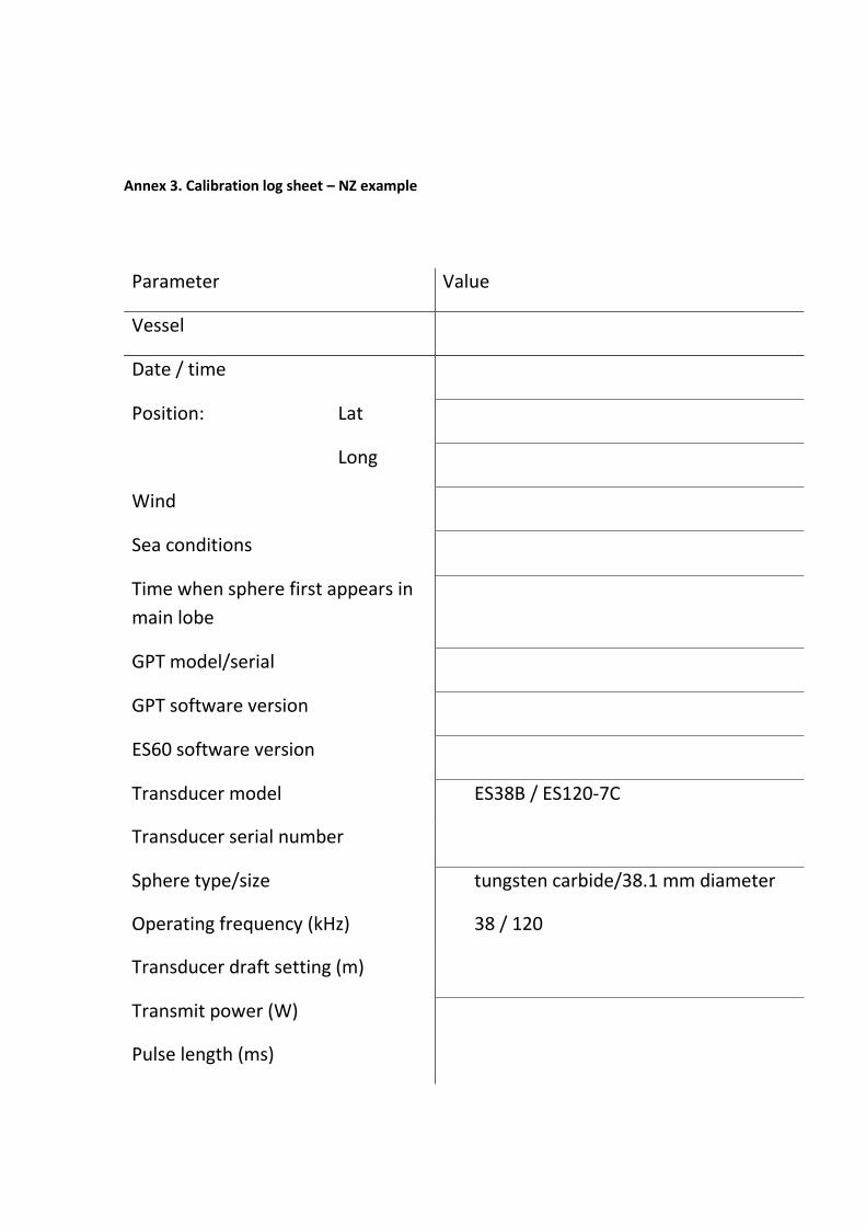
Annex 3. Calibration log sheet – NZ example
Parameter Value
Vessel
Date / time
Position: Lat
Long
Wind
Sea conditions
Time when sphere first appears in
main lobe
GPT model/serial
GPT software version
ES60 software version
Transducer model ES38B / ES120-7C
Transducer serial number
Sphere type/size tungsten carbide/38.1 mm diameter
Operating frequency (kHz) 38 / 120
Transducer draft setting (m)
Transmit power (W)
Pulse length (ms)

Transducer peak gain (dB)
Sa correction (dB)
Bandwidth (Hz)
Sample interval (m)
Two-way beam angle (dB)
Absorption coefficient (dB/km)
Speed of sound (m/s)
Angle sensitivity (dB)
alongship/athwartship
3 dB beamwidth (º)
alongship/athwartship
Angle offset (º)
alongship/athwartship
Calibration narrative / comments
e.g. Depth of sphere, changes in echosounder settings during experiment, changes in
position of sphere with time, etc.

Annex 4. ECHOVIEW Algorithms
Echoview offers a modular access to a wide variety of powerful tools and algorithms to be
used for calibration, removing noise and interference.
to. Calibration algorithm "SNP_1" (see Figure 10)
b. Noise removal algorithm "SNP_2" (see Figure 8 and Figure 11)
c. Algorithm for interference removal "SNP_3" (see Figure 9 and Figure 12)
Algoritmo de calibración “SNP_1”

Algoritmo eliminación de ruido “SNP_2”
Algoritmo eliminación de interferencia “SNP_3”

Annex 5 – Examples of noise
The images below are taken from section 8.6.1.1 of the Great Lakes acoustic survey SOP and
illustrate the types of noise that may be encountered while collecting calibration data.
A common type of acoustic noise is a discreet spike caused by another echosounder or sonar
operating within the frequency bandwidth or a harmonic of the scientific echosounder (Figs.
12a, 12b). The solution is to identify the source of the interference and shut it down.
Interference can also be eliminated if acoustical instrumentation essential for safe ship operation
is synchronized with the survey echosounder. Removal of acoustic noise during data analysis is
sometimes possible, but difficult, so eliminating it during the survey is always preferable
(Advanced Sampling Technologies Working Group 2003).
Fig. 12a. Example of acoustic interference (cross-talk) between two frequencies (diagonal lines,
indicated by arrow): a 70 kHz scientific transducer and 50 kHz on-boat depth-sounder.
Fig. 12b. Example of acoustic interference (cross-talk) between two frequencies
(unsynchronized 70 and 200 kHz scientific echosounders). The black arrows indicate
the appearance of cross-talk (horizontal lines) and the hollow arrow indicates an echo
return from side lobes hitting the hull of the survey vessel (solid, horizontal line in the
upper water column).

Annex 6. Electrical Noise
Electrical noise (interference, Figs. 13a, 13b) can be caused by improper grounding of the survey
echosounder or other components of the electrical system and can result in low-level voltage
interference, spikes, or cyclical interference. There is also some internal noise generated by
the electronics in the echosounders themselves. A low-level voltage introduced to the
echosounder will be amplified with range by the TVG function and pose a problem, mainly in
the greater depths of the survey area. Hydraulic pumps or winches may cause dramatic
increases in noise during operation and should be checked to ensure that they do not generate
noise during standby. It is advisable to test acoustics equipment under various operational
scenarios (e.g., winch operation, trawling, coffee maker turned on, galley fans, etc.) prior to
the commencement of a survey. It is also good practice to test equipment after significant
modifications to the vessel (e.g., winch, propeller, or generator replacement/repair). The
magnitude of these noise sources can change with vessel speed (see below). Electrical noise
can be reduced or eliminated by:
Ensuring proper grounding of the scientific echosounder
Using an uninterruptible power supply for the scientific echosounder
Placing transducer cables and data ethernet cables away from possible
electric fields, such as fluorescent lights
Electrical interference not eliminated during data collection (Figs. 13a, 13b) should be
removed during data analysis, either manually or with signal processing techniques. Manual
removal of noisy regions and excluding them from the analysis should not affect results, as
long as these regions are relatively small. Automated techniques may be possible but probably
require specialized software. If signal-processing techniques are used, care should be taken
to ensure that data are not modified or correction factors may be required.
Fig. 13a. Common noise pattern as seen on a 70 kHz acoustic echogram showing electrical interference
(arrow indicating the electrical wave-like pattern throughout much of the water column).

Fig. 13b. Common noise pattern as seen on a 70 kHz acoustic echogram showing noise from hydraulic
winches (arrow indicating vertical spikes) during trawl deployment.
Annex 7. Intercalibration
The capacity of a ship to provide acoustic information on the fish surveyed depends on several
factors:
- The calibration characteristics of the acoustic devices, this has been documented in this
document;
- The signal to noise ratio of this ship. A very noisy ship will have a bad signal to noise ratio
and therefore a poor capacity to record all the echoes of the fish population surveyed.
- A “ behavioral impact” which is the magnitude of avoidance reaction of the fish to this
particular vessel.
Therefore it can be important to intercalibrate two vessels in order to evaluate the bias
induced by these characteristics when gathering the data of the two ships. Such measurement
requires the two ships being calibrated prior to the intercalibration experiment.
Another reason of intercalibrating is when a ship cannot be calibrated for any reason
(availability, type of echo sounder, cost of the operation, etc.) Then intercalibration is a way to
allow taking into consideration the data collected by the uncalibrated ship, although the fact
that it is not calibrated does not allow to give to these data the same weight as those collected
aboard calibrated data.
As a general rule, when two or more boats sre used it is appropriateto perform an intercalibration. Such
experiment consists in making the ships operating over parallel transects close to each other (e.g. 30 to
50 m) for a period at least over two hours at speed work (10 knots), using when possible similar settings,
assuming that both vessels willrecord similar acoustic detections. Their respective results should be
identical, and the linear difference between them represents the correction factor to apply in order to
make them fully comparable The correlation between the NASC measurements should be ideally greater
than 0.90, otherwise the test should be repeated, or the reason explaining the discrepancy should be
found, or decision should be taken not to compare data from these ships
Procedure for intercalibrating digital echo sounders with Echoview software.
An essential requirement is that at least one of the two vessels, must be calibrated.
b. Set the path in which intercalibration go be performed, ideally the environment in which it will develop
should be fairly homogeneous, with scattered biomass (avoid shoals).
c. Echosounder operate in active mode at the same frequency and power, and calibrated.
d. The vessels must be synchronized by radio to start and stop recording at the same time (to calculate
averages comparable NASC), echo sounders should have the same date and GPS position.
e. The boats must navigate in parallel next to each other (30 to 50 m) for two hours at least.

f. Intercalibration save data on a USB device.
g. Echoview upload data to load the page corresponding to each boat calibration and export detections,
scanning lines is (1 m from the surface and -1m of the bottom line).
h. The end result of the intercalibration should be a graph of NASC detected by each vessel with intervals.
It is intended that the acoustic detections reflect similar measurements between the two ships through a
linear relationship. The correlation between the NASC measurements should be greater than 0.90,
otherwise the test should be repeated, or be the reason to explain the discrepancy.
Note: You can expect a correlation equal to unity because it is materially impossible for ships to sail on
the same scatterers (plankton, fish).

Annex 8. Noise level
Cuando la medición se ha completado, el nivel de ruido correspondiente (NL) se puede
calcular mediante el método de PN (dB re 1 uPa) , el cual consiste en medir la potencia del
ruido de fondo para cada ping (dB).
PN: 𝑁𝐿 = 𝑃𝑁 − 20𝑙𝑜𝑔𝜆 − 𝐺 + 192.8
|ecuación 1
PN es el Sv de cada ping (dB), λ es la longitud de onda (C/f) donde C es la velocidad del sonido
(m.s-1) y f es la frecuencia (Hz). G es la ganancia Sv del transductor (dB)
Una estimación del nivel máximo del ruido tolerable fue sugerida por el ICES ( ICES CRR 209,
1995|); se recomienda la siguiente ecuación para calcularlo:
𝑁𝐿 = 1330 − 22𝑙𝑜𝑔𝑓
ecuación 2
NL es “Noise Level” o nivel de ruido; f es la frecuencia empleada.

Anexo 91: “Ficha de calibración”.
Figura 1: Ejemplo de ficha de calibración de una ecosonda digital split beam, de 120 kHz.
FICHA DE CALIBRACION 120 khz -barco 1Callao 06 de agosto del 20156 a 13 horas
Frecuencia 120 kHz
Largo de pulso: 0.512 ms
Ancho de banda: 6.89 kHz
Potencia máxima: 1000 w
Potencia transmitida: 500 w
Sensitivida longitudinal: 23 °
Sensitividad transversal: 23 °
Transductor, blister ligeramente a estribor: ES120-7C
-3dB ancho de banda longitudinal según tabla: 6.9 kHz
-3dB ancho de banda transversal según tabla: 6.9 kHz
ángulo del haz equivalente en dos vías -20.9 dB
VELOCIDAD DEL SONIDO
temperatura media hasta la esfera 17.42 °C
salinidad media hasta la esfera 35.11 ups
Profundidad esfera 'r' 8.00 m
Coef. de absorción 38.00 dB-Km
Coef. de absorción 0.038 dB/mResultado 1529.19 m/seg.
TS ESFERATS esfera -40.40 dB
CALCULO PARA EL SA TEORICO
σ bs 9.12011E-05 m2Ψ -20.9 dB ref 1 strΩ 0.008128305 strr 8.00 m
SA(theory) 7556.34633 m2/mn2
NUEVA GANANCIA Sv DEL TRANDUCTOR
Old transd. gain 27.00 dBSA (measured) 2,501.40 m2/mn2
New transd. gain 24.60 dB
CONSTANTE DEL INSTRUMENTO Sa(m)/Sa(t)
TS -40.40 dB
Sa prom 7,547.20 m2/mn2
r 8.00 m
Resultado 0.99879 sin unidades

Annex 10. Calibration kit.
(This is an example from N-Z team, which can differ for each country depending on the
material and tools available)
3 x reels with 100 m of spectra on each (in NZ, use of Penn 330 reels)
2 x 38.1 mm tungsten carbide calibration spheres with attached
spectra
1 x flat blade screwdriver
1 x Phillips blade screwdriver
1 x 10 mm spanner
1 x retractable Stanley knife
1 x side cutters
Bunch of 200 mm long cable ties (at least 12)
6 x nut/bolt/washer sets for bolting poles together
4 x 30 mm spherical lead sinkers with attached spectra
2 x 750 g oblong lead weight with 3 m of attached spectra and hooked
swivel on the end of the spectra
1 x 2 m loop of 30 kg nylon
1 pack of spare 20 kg swivels
1 pack of spare hooked 20 kg swivels
A quantity of white cord
1 x bag of Penn reel manual, spanner and miscellaneous
documentation
1 reel of spare 30 kg nylon
1 reel of spare spectra
1 x laminated sphere netting instructions
1 x laminated calibration and ES/EK60 operating procedures
5 x ES/EK60 calibration log sheet
Weight: preferably small heavy cylinder around 1 kg.

Annex 11.
Equation of the sound velocity (MacKenzie, 1981)
C = 1448.96 + 4.591 * Tº - 5.304 * 0.01 * Tº2 + 2.374 * 10-4 * Tº3 + 1.34 * (S - 35) + 1.63
* 0.01 * R + 1.675 * 10-7 * R +- 1.025 * 0.01 * Tº * (S-35) – 7.139 * 10-13 * Tº * R3