report no.: escml 07-04 report title: moca user’s … · 7.2.1 loading poet files into moca 7-8...
TRANSCRIPT

ESCML Technical Report 07-04
CALCE Electronic Products and Systems Center • Building 89, Room 1103 • University of Maryland College Park, MD 20742 • ph: 301-405-5323 • fax: 301-314-9269 • www.calce.umd.edu
Report No.: ESCML 07-04 Report Title: MOCA User’s Guide, V. 2.3 Principal Investigator: P. Sandborn Abstract: This report is a user’s guide for the Mitigation of Obsolescence Cost Analysis (MOCA) software tool Version 2.3. MOCA determines the part obsolescence impact on life cycle sustainment costs for long field life electronic systems based on future production projections, maintenance requirements and part obsolescence forecasts. The methodology uses a detailed cost analysis model to determine the optimum design refresh plan during the life cycle of the product (design, production, and operation and support). The design refresh plan consists of the number of design refresh activities, their respective calendar dates and content. The methodology supports user determined short- and long-term obsolescence mitigation approaches on a per part basis, variable look-ahead times associated with design refreshes, and allows for inputs to be specified as probability distributions. Inputs can be loaded from spreadsheets, the Frontier Technology ICE tool, the QTEC QStar tool, or the Titan Poet environment. Outputs from MOCA can optionally be used as inputs to the PRICE Systems PRICE H/L commercial software tools for predicting more extensive life cycle costs of systems. This user’s guide is a complete documentation of the “Default”, “ICE” and “POET” MOCA operating modes. The MOCA “Development” operation mode is not documented in detail herein, but is described in an Appendix.
Electronic System C
ost Modeling Laboratory
(CA
LCE Electronic Products and System
s Center)
Electronic System C
ost Modeling Laboratory
(CA
LCE Electronic Products and System
s Center)

ESCML Technical Report 05-02
Electronic Systems Cost Analysis Laboratory • Department of Mechanical Engineering • University of Maryland
College Park, MD 20742 • ph: 301-405-3167 • fax: 301-314-9477 • www.enme.umd.edu/ESCML
Unless otherwise indicated, this is considered a draft report
Revision History
Contributor Date Description
Sandborn June 21, 2007 Initial version of report created
CALCE Contact: Reviewed and Approved: ______________________ _________________
(signature) (date)
Content Disclaimer
The information contained in this document is designed to be accurate and authoritative in regards to the subject matter covered. However, it is provided with the understanding that the provider is not engaged in
rendering legal, accounting, engineering, or other professional services. The Electronic System Cost Modeling Laboratory (ESCML) and the CALCE Electronic Products and Systems Center (EPSC)
disclaims any responsibility or liability for this material and is not responsible for the use of this information outside of its educational purpose.
Copyright Notice
The information contained within this report has been developed by the
University of Maryland, the Electronic System Cost Modeling Laboratory (ESCML) and the CALCE Electronic Products and Systems Center (EPSC).
Replication rights of all information is retained by the
CALCE Electronic Products and Systems Center.
Copyright © 2007 CALCE EPSC and the University of Maryland. All rights reserved.

Table of Contents
i
Table of Contents
1 – Introduction 1-1 1.1 The Mitigation of Obsolescence Cost Analysis (MOCA) Tool 1-1 1.2 MOCA Design Flow and Architecture 1-1 1.3 Introduction to this Manual 1-4 1.4 Reference Materials 1-5
1.4.1 Related Documentation 1-5 1.4.2 MOCA Acknowledgements 1-5 1.4.3 Getting Additional Help 1-5
2 – Installation 2-1 2.1 Downloading MOCA from the Web 2-1
2.2 Installation on a Windows Machine 2-2 2.3 Using the MOCA install.exe File 2-3
3 – MOCA Tutorial Example 3-1 3.1 Starting MOCA 3-1 3.2 MOCA Data Requirements 3-2 3.3 Loading Board-Level Data 3-3 3.4 Component Data 3-5 3.5 Board Data 3-7 3.6 Design Data 3-8 3.7 Production Data 3-10 3.8 Solution Control Data 3-10 3.9 Performing a MOCA Analysis and Viewing Design Optimization
Results 3-12 3.10 Saving the Design 3-14 4 – MOCA Input Reference 4-1 4.1 Part (Component) Input Reference 4-1
4.1.1 Obsolescence Mitigation Models 4-4 4.1.2 Part-Specific Technology Trends Parameters 4-10
4.2 Board Input Reference 4-11 4.2.1 Parts (Bill of Materials) for the Board 4-12 4.2.2 Board Properties 4-13 4.2.3 Design Hierarchy 4-15 4.3 System (Design) Input Reference 4-15 4.3.1 Qualification Levels 4-17 4.4 Production Input Reference 4-19 4.4.1 Production Quantities 4-21 4.5 Constraints Inputs Reference 4-22
4.6 Solution Control Input Reference 4-22 4.6.1 Monte Carlo Analysis 4-22 4.6.2 Cost Analysis 4-24

MOCA User’s Manual, Version 2.3
ii
4.6.3 Other System Control Inputs 4-24 4.7 System Setup Input Reference 4-26 4.8 Part Synthesis Solution Control Reference 4-29 4.8.1 Maturity of Synthesized Parts 4-29 4.8.2 Reliability of Synthesized Parts 4-29 4.8.3 Lifetime of Synthesized Parts 4-30 4.9 Probability Distribution Input Reference 4-30 4.9.1 Probability Distribution Inputs for Table Data 4-31 4.9.2 Probability Distribution Inputs for Other Data 4-31 4.10 MOCA Menu Command Reference 4-32 5 – MOCA Input File Reference 5-1 5.1 Board Data File Reference 5-1 5.2 Component Data File Reference 5-3
5.3 Importing TACTech Lifecode Indices 5-5 5.4 Production Event File Reference 5-5
6 – MOCA Outputs 6-1 6.1 Results Graph 6-1 6.1.1 Interpretation of the Horizontal Axis 6-4 6.1.2 Changing Plot Scales 6-5 6.2 Cost (Timeline) Graphs 6-7
6.3 The Design Refresh Plan 6-9 6.4 Business Case Analysis 6-10 6.4.1 Obsolescence Management Cost 6-10 6.4.2 Running the MOCA Business Case Analysis 6-11
6.5 Uncertainty Analysis 6-13 6.5.1 Running Monte Carlo Analysis for Individual Refresh Plans 6-13
6.5.2 Running Monte Carlo Analysis for an Entire Design Refresh Optimization 6-15
6.6 Applying Solution Constraints 6-16 6.6.1 Defining Roadmapping Constraints 6-16 6.6.2 Defining Budget Constraints 6-18 6.7 Computing Confidence Levels 6-20
7 – Integration with Other Tools 7-1 7.1 Frontier Technology, Inc. ICE Tool 7-1 7.1.1 Loading ICE Files into MOCA 7-1 7.1.2 ICE File Format and Reference 7-2 7.1.3 The ICE Menu 7-6 7.2 Titan Poet Environment 7-8 7.2.1 Loading Poet Files into MOCA 7-8 7.2.2 Poet File Format and Reference 7-9 7.2.3 The Poet Menu 7-13 7.3 Price H and HL Tools 7-14

Table of Contents
iii
7.4 Q-Star Integration 7-15 7.4.1 Q-Star Reports 7-16 7.4.2 Loading Q-Star Reports into MOCA 7-17 Appendix A – Definitions A-1 Appendix B – MOCA Date Conversion B-1 Appendix C – Obsolescence Mitigation Factor Calculation C-1 C.1 Model Construction C-1 Appendix D – Refresh Selection Algorithm D-1 Appendix E – MOCA Input Requirements Summary E-1 Appendix F – Description of MOCA “Development” Mode F-1 F.1 Technology Insertion MOCA F-1 F.1.1 Using the Technology Insertion Version of MOCA F-3 F.2 NSWC Horizon Integration F-4 F.3 Synthesizing Floating Obsolescence Dates F-4 F.4 Weeding Out Unused Boards F-5 F.5 Obsolescence Case Resolution Costs F-5 F.6 Part Type Controllable Obsolescence Dates F-5 F.7 Accumulating Obsolescence Events F-6 F.8 Miscellaneous Additional Menu Commands F-8

Blank Page

Chapter 1 - Introduction
1-1
CHAPTER 1 - Introduction The rapid growth of the electronics industry has spurred dramatic changes in electronic parts. Increases in speed, reductions in feature size and supply voltage, and changes in interconnection and packaging technologies are becoming events that occur almost monthly. Consequently, many of the electronic parts that compose a product have life cycles that are significantly shorter than the life cycle of the product. This life cycle mismatch problem requires that during design, engineers be cognizant of which parts will be available and which parts may be obsolete during a product’s life. This problem is especially prevalent in avionics and military systems, where systems may encounter obsolescence problems before being fielded and nearly always experience obsolescence problems during their field life. This problem is exacerbated by manufacturing that takes place over long periods of time, and the high cost of system re-qualification that makes the design refreshes extremely expensive.
Many part obsolescence mitigation strategies exist including: life time buy, last-time buy, part replacement, aftermarket source, uprating, emulation, re-engineering, reclaim, and ultimately redesign of the system. Design refresh (or redesign) has the advantage of treating multiple existing and anticipated obsolescence problems concurrently and additionally allows for functional upgrades. Unfortunately, design refresh is also often a very expensive option, not just in non-recurring engineering costs, but also in potential system re-qualification costs. 1.1 The Mitigation of Obsolescence Cost Analysis (MOCA) Tool
A methodology and it’s implementation (MOCA) has been developed for determining the part obsolescence impact on life cycle sustainment costs for the long field life electronic systems based on future production projections, maintenance requirements and part obsolescence forecasts. Based on a detailed cost analysis model, the methodology determines the optimum design refresh plan during the field-support-life of the product. The design refresh plan consists of the number of design refresh activities, their respective calendar dates and content to minimize the life cycle sustainment cost of the product. The methodology supports user determined short- and long-term obsolescence mitigation approaches on a per part basis, variable look-ahead times associated with design refreshes, and allows for inputs to be specified as probability distributions that can vary with time. Outputs from this analysis can optionally be used as inputs to the PRICE Systems PRICE H/L commercial software tools for predicting life cycle costs of systems. 1.2 MOCA Design Flow and Architecture Figure 1.1 summarizes the MOCA methodology for making value-based decisions about how to refresh a sustainment-dominated system’s design. MOCA determines the best dates for design refreshes, and the mixture of actions to take at the design refreshes. The methodology can be used during either: a) the original product design process, or b) to make decisions during system sustainment, i.e., when a design refresh is underway,

MOCA User’s Manual, Version 2.3
1-2
determine what the best set of changes to make given an existing history of the product and forecasted future obsolescence and future design refreshes. The obsolescence dates for the chosen technologies (e.g., electronic parts), are forecasted. Note, MOCA does not perform obsolescence forecasting, forecasts must be supplied to MOCA as an input. The forecasts will most generally be in the form of a probability distribution whose shape depends on the forecasting method used. The other type of the information necessary to make decisions about how to modify a design at design refreshes comes from production information. From the design process, an anticipated production plan (quantity that need to be manufactured as a function of time) is used along with a forecast of the number of spare products that will need to be produced to replace product that fails in the field during the product’s usage life. Remember we are dealing with sustainment-dominated products that will fail in the field due to wearout and overstress, and will require replacement. The production plan associated with “spare replenishment” is determined from the forecasted reliability of the product’s components and the forecasted usage profile for the system. Using a production plan, viable locations for design refreshes can be determined. With the viable design refresh dates chosen; a candidate refresh plan can be formed. A refresh plan is a group of one or more design refreshes representing all the refreshes (and their respective dates) that will be performed on a product during its lifetime. Armed with obsolescence forecasts, the production plan and a candidate design refresh plan, we now determine the life cycle cost of the product subject to the candidate refresh plan by traversing the timeline and costing the events as they occur. To determine the “best” design refresh plan, multiple candidate refresh plans can be assessed. For sustainment-dominated products, the number of discrete production events is usually
Production Plan
Product Design and Planning
Forecast Obsolescence
•Technology/Part Selections
•Production schedule
Usage scenarioReliability
•Spare requirements
•Production plan (quantity and schedule)
Choose Refresh Candidates
•Valid Refresh Dates
Select a Candidate Refresh Plan
•Plan (multiple refresh dates)
•Obsolescence Dates Budget Constraints
Next candidate plan
“Best” Design Refresh Plan• Design Refresh Dates• Design Refresh Content (what
technologies/parts to change)
• Minimize life cycle cost• Maximize “value”
(performance, reliability, etc.)
•Production plan
Construct a Timeline (Figure 3)
Determine Life Cycle Cost of the Timeline
•Timeline (corresponding the candidate refresh plan)
•Life cycle cost (corresponding the candidate refresh plan)
Determine Design Changes at Refreshes
(Figure 5)•Part data•Obs. mitigation data•Value data
Figure 1.1 – MOCA methodology for making value-based decisions about how to
refresh a sustainment-dominated system’s design.

Chapter 1 - Introduction
1-3
relatively small (5 to 10 is not unusual), so checking all possible candidate refresh plans is not out of the question. A sample timeline for an electronic product is shown in Figure 1.2. Fundamentally, the methodology must support a design through periods of time when no parts are obsolete, followed by multiple part-specific obsolescence events. When a part becomes obsolete, some type of mitigation approach must take effect as soon as additional parts are required - either a lifetime buy of the part is made1 or a short-term mitigation strategy that only applies until the next design refresh. Next there are periods of time when one or more parts are obsolete, lifetime buys or short-term mitigation approaches are in place on a part-specific basis. When design refreshes are encountered, the change in the design at the refresh must be determined and the costs associated with performing the design refresh must be computed. At a design refresh a long-term obsolescence mitigation solution is applied (until the end of the product life or possibly until some future design refresh), and non-recurring, recurring, and re-qualification costs computed. Re-qualification may be required depending on the impact of the design change on the application – the necessity for re-qualification depends the role that the particular part(s) play and the volume of non-critical changes made. If the expense of a redesign is to be undertaken, then most likely, functional upgrades will also occur during the redesign. The system functional upgrades must be forecasted, including forecasting the obsolescence of future parts (any part replacement made at a refresh will be with a part that will eventually become obsolete too!). All the design refresh activities have to accommodate both hardware and software redesign and re-qualification. The last activity appearing on the landscape is production. The product often has to be produced after parts begin to go obsolete due to the length of the initial design/manufacturing process, additional orders for the product, and replenishment of 1 Enough parts are purchased to satisfy the product’s forecasted production and sustainment needs through the end of the product’s life.
Start of Life
Part becomes obsolete
Part is not obsolete Part is obsolete short term mitigation strategy used
Design refresh
• Spare replenishment• Other planned production
“Short term” mitigation strategy
• Existing stock• Last time buy• Aftermarket source
• Lifetime buy
“Long term” mitigation strategy
• Substitute part• Emulation• Uprate similar part
Redesign non-recurring costs
Re-qualification?• Number of parts changed• Individual part properties
Functionality Upgrades
Hardware and Software
Figure 1.2 – High-level overview of MOCA’s functionality. Note, MOCA Version 2.3 does not support software changes at design refreshes.

MOCA User’s Manual, Version 2.3
1-4
spares. When the timeline is costed, obsolescence events (or really their associated short-term mitigation) modify the recurring cost of the product the next time it is manufactured. Production events change recurring manufacturing costs to the life cycle total, and design refresh events modify the recurring cost of the product the next time it is manufactured and charge non-recurring redesign and re-qualification costs to the life cycle total.
MOCA features include:
• Monte Carlo analysis – every input can be represented by a probability distribution, results are probability distributions
• Variable look-ahead time • User controllable time-step fidelity • Supports fixed functional design refreshes (in addition to the obsolescence drive
design refreshes solved for by the tool) • Redesign “blackout” periods of time (periods when redesigns are not allowed) • Broad range of obsolescence mitigation approaches and mitigation models • User controllable re-qualification costs and criteria • Automatic business case generation • Automatic incorporation of solution time and cost constraints • Various tool integrations to support importing obsolescence risk, and performing
cost modeling. 1.3 Introduction to this Manual This manual is a reference intended for all MOCA users. This document contains the following chapters: Chapter 2: Installation – provides instructions on obtaining and installing the MOCA
software application from CD and from website download. Chapter 3: MOCA Tutorial Example – provides a detailed walkthrough of how the
MOCA tool using a design example provided with the MOCA installation. Chapter 4: MOCA Input Reference – reference for all MOCA input fields and buttons. Chapter 5: MOCA Input File Reference – explains the format of the spreadsheet files
that can be used to input board and component data into MOCA. Chapter 6: MOCA Outputs – summary of all MOCA output formats (plots and reports)
including interpretation of the results. Chapter 7: Integration with Other Tools – Describes the integration of MOCA with the
Frontier Technology ICE tool, the Titan Poet environment, the Price Systems tools, and the QTEC QStar tool.
Appendix A: Definitions – explanation of terminology used in the MOCA tool.

Chapter 1 - Introduction
1-5
Appendix B: MOCA Date Conversion Appendix C: Obsolescence Mitigation Factor Calculation Appendix D: Refresh Selection Algorithm Appendix E: MOCA Input Requirements Summary Appendix F: Description of the MOCA “Development” Mode 1.4 Reference Materials 1.4.1 Related Documentation P. Singh and P. Sandborn, "Obsolescence Driven Design Refresh Planning for Sustainment Dominated Systems," Engineering Economist, Vol. 51, No. 2, pp. 115-139, April-June 2006.
J. Myers and P. Sandborn, "Integration of Technology Roadmapping Information and Business Case Development into DMSMS-Driven Design Refresh Planning of the V-22 Advanced Mission Computer," Proceedings of the 2007 Aging Aircraft Conference, Palm Springs, CA, April 2007.
P. Singh, P. Sandborn, T. Geiser, and D. Lorenson, "Electronic Part Obsolescence Driven Design Refresh Planning," International Journal of Agile Manufacturing, Vol. 7, No. 1, pp. 23-32, 2004. MOCA Software Tool Download Page (available at: http://www.calce.umd.edu/contracts/MOCA/MOCA_Page.htm) 1.4.2 MOCA Acknowledgements MOCA development work has been funded in part by the Air Force Research Laboratory and Wright-Patterson AFB, sponsored by the ManTech Sustainment Initiative, Manufacturing for Sustainment under contract F33615-99-2-5503; the CALCE Electronic Products and Systems Center. 1.4.3 Getting Additional Help Technical support for this version of MOCA can be obtained from the University of Maryland by contacting: Peter Sandborn (301) 405-3167 [email protected] www.enme.umd.edu/ESCML

Blank Page

Chapter 2 - Installation
2-1
CHAPTER 2 - Installation This chapter describes the installation process for MOCA. Note, MOCA was developed on a Windows machine and only Windows machines are supported at this time. MOCA is designed to operate standalone, or with any of several other software tools discussed in Chapter 7. The installation of the tools discussed in Chapter 7 is not treated in this document. 2.1 Downloading MOCA from the Web MOCA can be downloaded from the MOCA web page at the following URL (Figure 2.1):
http://www.calce.umd.edu/contracts/MOCA/MOCA_Page.htm The web page is publicly accessible, but a password is required in order to download the software or documentation.1 Several versions of MOCA are available on the web site, scroll to the top of the table to access the latest version.
1 Contact Peter Sandborn ([email protected], 301-405-3167) to inquire about access.
Figure 2.1 – MOCA download page.

MOCA User’s Manual, Version 2.3
2-2
2.2 Installation on a Windows Machine If you received the MOCA tool on a CD, copy the MOCA-2.3 folder2 off the CD and onto the top-most level your C drive, i.e., its address should be C:\MOCA-2.3, then proceed to step 2. If you received MOCA via a download or email follow the steps below starting with step 1. 1) Unzip MOCA-2.3.zip by double clicking on it (make sure that the unzipped folder, MOCA-2.3 is located at the top-most level your C drive, i.e., its address should be C:\MOCA-2.3). Important: also make sure that your unzip utility has not “flattened” the file structure by default. 2) Create a folder called C:\moca and copy invokeprice.exe, price_ping.exe, and refresh_txt.bat from the C:\MOCA-2.3\current_moca_6 folder into it. 3) If you are planning to MOCA in conjunction with Price Systems tools complete the following:
WINNT (Windows NT including Windows 2000 and Windows XP) users: A batch file named regdll.bat is located inside the MOCA-2.3\current_moca_6 folder. Double click on it. This registers the DLL’s used by MOCA.3 Non-WINNT (Windows 95 and 98) users: Choose Run from the Start menu and type in regsvr32 "C:\ MOCA-2.3\current_moca_6\PRICE_PASES.dll"4
4) There is a folder called “current_moca_6” inside MOCA-2.3. This folder contains a file named “current_moca_6.exe”. Double clicking on current_moca_6.exe will startup the MOCA tool. You may create a shortcut to this executable for placement on your desktop. You must not move the current_moca_6.exe out of the MOCA-2.3/current_moca_6 folder. Once MOCA is properly loaded and executed two opening screens will appear (see Figure 2.2).
2 Note, your folder may have a slightly different name depending on what version of the tool you have, e.g., MOCA-2.3.5 for example. 3 Note, if you want to locate your MOCA-2.3 folder someplace other than the top-most level of your C drive, click the right mouse key on regdll.bat and choose Edit from the menu. Change the line regsvr32 "C:\ MOCA-2.3\current_moca_6\PRICE_PASES.dll" to reflect the location of the MOCA-2.3 folder. When you resave the regdll.bat file you may have to provide a different name as it may be a “read only” file. 4 Note, if you have located your MOCA-2.3 folder someplace other than the top-most level of your C drive, change this line to reflect the location of the MOCA-2.3 folder. Click OK.

Chapter 2 - Installation
2-3
2.3 Using the MOCA install.exe File The install.exe file provided along in the MOCA .zip file can be used for a single click installation of MOCA on a PC. This program copies files: invokeprice.exe, ping_price.exe, and refresh_txt.bat into the C:\moca folder. If this folder already exists, it prompts the user for overwrite/skip options, otherwise it creates a new folder and copies the required files into it. Also, an icon for MOCA is created on the user’s desktop, which can then be clicked to start the currently installed version of MOCA. Note: once the MOCA .zip file is unzipped, if the location of the unzipped folder is changed the MOCA icon on the desktop will no longer operate correctly.
Figure 2.2 – MOCA opening screens. Note the title on the black DOS window and the content printed in the black DOS window will vary depending on whether the
MOCA executable is started from a shortcut or by double clicking the actual executable.

Blank Page

Chapter 3 - MOCA Tutorial Example
3-1
CHAPTER 3 – MOCA Tutorial Example This chapter provides a quick tour through the major portions of the MOCA user interface. First time users can complete this example to familiarize themselves with the primary functions of MOCA and the MOCA interface. Definitions of the terminology used in this chapter are found in Appendix A and Chapter 4 provides a complete reference to the MOCA dialog boxes, menu items, and input fields. This tutorial is an example of calculating the optimal redesign plan for an example system consisting of three boards and approximately 4000 parts. The user will begin by loading files describing each of the boards into the MOCA tool. After observing the inputs associated with the boards and components in the MOCA interface, users will run an optimization that computes the effective life cycle cost for all design refresh options up to and including a total of four redesigns in the product’s life. 3.1 Starting MOCA Once MOCA is properly loaded and executed the opening screens will appear (Figure 3.1). Installing and starting the MOCA tool are covered in Chapter 2. The two screens that appear are a DOS (black) window on which various MOCA status messages will be printed and a MOCA Version dialog box.1
1 Depending on the particular version of MOCA you are running and the way MOCA was initiated, the black DOS window may or may not appear and the MOCA version number may vary.
Figure 3.1 – MOCA opening screens.

MOCA User’s Manual, Version 2.3
3-2
To start MOCA for normal use, press the <OK> button on the MOCA Operating Mode dialog box. The MOCA title screen shown in Figure 3.2 will appear. This title screen will be the starting point for most MOCA analyses.
3.2 MOCA Data Requirements MOCA requires five different types of data to perform its analysis:
• Design Data (Section 3.6) – a design is the “container” that holds all the boards in the system. The design is sometimes referred to as the “box”. The design may be hierarchical (boards contained within boards). Qualification levels and costs are by default defined at the design level. Default redesign cost modeling inputs are also defined at the design level.
• Board Data (Section 3.5) – boards represent electronic substrates with one or more components (parts) attached to them and possibly other boards hierarchically defined within them. The list of actual parts and the number of instances of the parts in the board. Qualification levels and costs can be defined at the board level. Reliability is defined at the board level. Sparing is performed at the board level.
• Component Data (Section 3.4) – global electrical components (parts) characteristics. The characteristics of components include their purchase price, obsolescence date, and obsolescence mitigation approach(es). A global database structure for parts is contained within MOCA, i.e., parts can be defined independent of whether they are actually used within any boards that comprise the design.
Figure 3.2 – MOCA title screen.

Chapter 3 - MOCA Tutorial Example
3-3
• Production Data (Section 3.7) – production data includes the schedule for manufacturing the design (how many units are made as a function of time). Also included within the production data is sparing requirements, prototypes, fixed redesign dates, dates when design refreshes will not be allowed, and the date on which the MOCA analysis should begin.
• Setup and Control Data (Section 3.8) – MOCA provides a wide range of solution control data and secondary inputs that can be manipulated by the user to tune the solution.
A concise summary of the MOCA input requirements is provided in Appendix E. 3.3 Loading Board-Level Data This section focuses on loading part information stored in data files that define individual boards. The files being loaded into MOCA are comma-delimited files (CSV format) created from a spreadsheet (see Chapter 5 for format). The files loaded in this section contain part information, specific part instance data associated with specific boards, and board characteristics. To load board files for evaluation:
1) Select the “Load Board File (.csv)” command from the File menu in the MOCA interface (select File->Load Board File (.csv)), see Figure 3.3. A Load Data File dialog window will appear (see Figure 3.4).
2) Navigate to the following directory in the file dialog box:
MOCA_2.3/current_moca_6/data/MTC. Select the board_3.csv file from the file browser and press the <Open> button (Figure 3.4). A warning message stating the design id does not exist will appear (see Figure 3.5). This message indicates that you have not explicitly created a new design to load the boards into. By pressing <Yes> in the Error/Warning dialog box, a new design will automatically be created.
Note, you could have invoked Inputs->Design Selection and pressed <Add New Design> to create a new design prior to loading the boards in order to avoid this warning message (see Section 4.3).
3) Repeat step 1 for the other two boards in the example, i.e., select File->Load
Board File (.csv), and load the board_1.csv and board_2.csv boards. When loading board files into MOCA, if duplicate component part numbers are encountered (either previously loaded, or appearing in the same file) an Action Window containing the warning message appears (see Figure 3.6). The functions of the various buttons is discussed in Table 3.1.

MOCA User’s Manual, Version 2.3
3-4
Figure 3.3 – Load Board File menu selection.
. Figure 3.4 – Loading the board_3.csv file.
Figure 3.5 – Design ID warning.

Chapter 3 - MOCA Tutorial Example
3-5
Table 3.1 – Duplicate component warning actions.
Button Result
Yes
The existing data (existing in MOCA’s internal component database for this design) will be overwritten with the new version of the component encountered in the file currently
being loaded.
Yes to all Will result in overwriting of the existing component information.
No
The existing data (existing in MOCA’s internal component database for this design) will not be overwritten with the
new version of the component encountered in the file currently being loaded.
No to all All instances of duplicate components (associated with the file currently being loaded) will not result in overwriting of
the existing component information. Note, only the component’s part number is checked for duplication. If you choose to overwrite existing components, their properties will be replaced with the properties of the newest version of the component. You should press <Yes to all> to continue the tutorial.
4) Loading an example design for analysis is completed by adding default
production details. From the Setup menu, select Setup->Default Production Data->0 - production: yearly. This generates default production schedule information (dates and quantities) to go with this example (see Sections 3.7 and 4.4 for more details).
The demonstration example continues in Section 3.9, however, you may wish to tour the MOCA interface and observe the data that was loaded in this section.
3.4 Component Data
The boards loaded in Section 3.3 contained all the part data for the parts that they package. The global part data can be viewed (and edited) by selecting the “Components
Figure 3.6 – Duplicate component warning dialog box.

MOCA User’s Manual, Version 2.3
3-6
Definition” command from the Inputs menu in the MOCA interface (select Inputs->Components Definition). A Parts dialog window will appear (see Figure 3.7).
The data columns for the parts description data table are discussed in detail in Section 4.1, but briefly,
Cost ($) = price per instance of the part Cost Dist. = probability distribution associated with the cost; left clicking produces a menu that offers the following distributions: None, Normal, Uniform, and Triangular. The characteristics of these distributions can be viewed by right clicking on the field. The distributions are only used if a Monte Carlo analysis is being used. Obs. Date = date of part obsolescence Obs. Date Dist. = probability distribution associated with the obsolescence date for the part; left clicking produces a menu that offers the following distributions: None, Normal, Uniform, and Triangular. The characteristics of these distributions can be viewed by right clicking on the field. The distributions are only used if a Monte Carlo analysis is being used. Obs. Mitigation = left clicking produces a dialog box that allows the form of the obsolescence mitigation for the part to be defined (see Section 4.1.1). Part Category = used to define the overall lifetime of today’s part. This information is used when MOCA synthesizes a replacement part for use after a future obsolescence event. Set Tech. Trends = parameters that model the part-specific effort necessary to change the part at a design refresh (see Section 4.1.2).
See Chapter 4 for detailed explanations of all the other data columns. Table 3.2 explains what occurs when the user selects a button in the parts dialog window.
Figure 3.7 – Parts dialog box.

Chapter 3 - MOCA Tutorial Example
3-7
Table 3.2 – Parts dialog box buttons. Button Result
Add Component
Adds a component to the table.
Delete Component(s)
Deletes a component from the table.
Clear Table Deletes all data in the table. Set
Obsolescence Mitigation Cost
Factors to Global
Sets the cost factors associated with selected obsolescence mitigation approaches to the global default values (see Chapter 4).
Create Reorder Creates an order of a specific part in the production details.
The “part_3” that appears in the Part Number column on the Parts Dialog is actually a group of parts that were determined to be uninteresting when the original board design was entered into the spreadsheet. By uninteresting, we mean that these are all the parts in the system that will not become obsolete and will not be functionally upgraded during the life time of this product. Note, lumping parts like this is not required to run MOCA, it is only done to accelerate the MOCA analysis. If you are lumping parts, the Cost is the total cost of all the parts, the Obs. Date should be set to a year that is well past the end of life of the product, and the Part Category should be set to “Assorted”. When you are finished viewing the component data, the dialog boxes may be closed by pressing either the <OK> or <Cancel> buttons. 3.5 Board Data
The board data loaded in Section 3.3 can be viewed (and edited) by selecting the “Boards Definition” command from the Inputs menu in the MOCA interface (select Inputs->Boards Definition). The three boards loaded in Section 3.3 appear in the Boards dialog window (see Figure 3.8).
Figure 3.8 – Boards dialog box.

MOCA User’s Manual, Version 2.3
3-8
The data columns for the boards dialog box are discussed in detail in Chapter 4, but briefly,
Quantity = number of instances of the board in the system Parts = clicking on this field produces a dialog box that allows the bill of materials for the board to be defined by selecting parts from the global database – Figure 3.9. Properties = clicking on this field produces a dialog box that allows the board properties to be viewed and edited. Modules = produces a dialog box identical to the one in Figure 3.8 where daughter boards of the selected board can be defined (see the design hierarchy discussion in Section 4.2.3).
When you are finished viewing the board data, the dialog boxes may be closed by pressing either the <OK> or <Cancel> buttons. 3.6 Design Data The design data loaded in Section 3.3 can be viewed (and edited) by selecting the “Design Selection” command from the Inputs menu in the MOCA interface (select Inputs->Design Selection). The Design Selection Dialog appears in Figure 3.10. Using this interface, specific designs can be selected or created (design 0 was created by MOCA when you loaded the board_3 board – Figure 3.5). In addition, the number of operating hours per year for the system is required (used for spare replenishment calculations), and if MOCA’s internal cost calculations are used to estimate design refresh non-recurring costs, and then several cost inputs are needed. Independent of the method used to model non-recurring costs, the qualification costs and levels must be defined.
Figure 3.9 – The parts list corresponding to the board_3 board. The Quantity column collects the number of instances in the board and the Qualification Levels
allows the specific qualification tests that the part impacts to be defined (see Section 4.3.1 for customization of the qualification levels).

Chapter 3 - MOCA Tutorial Example
3-9
MOCA defaults to system level qualification, however, qualification can be performed at the board level instead (see Section 4.6 for instructions on controlling the level at which qualification performed). The Re-Qualification Cost field collects the total qualification cost for the system. By clicking on the <Set Qualification Levels> button, the Qualification Levels Dialog box appears, Figure 3.11. This dialog box allows users to define specific qualification levels (Non-EMI and Non-EMI + EMI are custom qualification levels that were loaded with this design). The cost of specific qualification level is defined as a fraction of the total Re-Qualification Cost that appears in Figure 3.10 (note, the fractions need not add up to 1.0). MOCA will also automatically trigger a full re-qualification if the number of non-critical component changes exceeds a specified count (200 in Figure 3.11). Once qualification levels are defined, specific parts can be
Figure 3.11 – Qualification Levels Dialog box.
Used for MOCA internal non-recurring design refresh cost model only
Qualification level and cost definition
Figure 3.10 – Design selection dialog box.

MOCA User’s Manual, Version 2.3
3-10
associated with them (Figure 3.9), i.e., if an associated part is changed at a design refresh then the qualification levels it is associated with are automatically performed at the design refresh. 3.7 Production Data The default production data loaded in Section 3.3 can be viewed (and edited) by selecting the “Planned Productions/Redesigns” command from the Inputs menu in the MOCA interface (select Inputs->Planned Productions/Redesigns). The Planned Productions/Redesigns Dialog appears in Figure 3.12. The production interface allows the dates of the start of analysis, the end of analysis (end of support date), and all production events. Beyond the original production quantity and date, each subsequent production event can be added to the table in the interface. The event type can be designated – general production events are called “Reorders”, but other production events are also possible, e.g., Spare Replenishments and Prototypes. The interface also allows fixed redesigns to be scheduled (MOCA will optimize around them), and periods of time when no redesigns are allowed. See Section 4.4 for detailed explanations of all the production inputs. 3.8 Solution Control Data The Solution Control Window (Figure 3.13) allows various parameters that control how the analysis is performed to be defined. The solution Control window is reached by selecting “Solution Control” from the “Setup” menu (Setup->Solution Control). Various categories of analysis control are available:
Figure 3.12 – Planned Productions/Redesigns dialog box.

Chapter 3 - MOCA Tutorial Example
3-11
Monte Carlo - When Monte Carlo analysis is enabled, probability distributions can be optionally used for the tool inputs instead of fixed values. MOCA defaults to Monte Carlo analysis off. See Sections 4.6.1 and 4.9 for an expanded discussion of the Monte Carlo analysis in MOCA. Cost Analsyis - The recurring and non-recurring costs associated with design refreshes in MOCA can be computed in several different ways making use of either internal cost models within MOCA or the Price Systems H/HL tools. MOCA defaults to using its own internal cost calculations. See Section 4.6.2 for more details. Functional Upgrades – Default analysis in MOCA considers only design refresh, i.e., one-for-one replacement of parts that are obsolescence risks. Functional upgrades allows MOCA to use trend analysis to perform functional upgrades on some portion of the system in addition to managing obsolescence risks. See Section 4.6.3 for more details.
The remainder of the solution control inputs are discussed in detail in Section 4.6.3.
Figure 3.13 – Solution Control Window.

MOCA User’s Manual, Version 2.3
3-12
3.9 Performing a MOCA Analysis and Viewing Design Optimization Results In this section a design analysis will be run by MOCA on the example data loaded in Section 3.3. MOCA automatically determines the reasonable design refresh plans by only analyzing those plans that could result in a minimum life cycle cost solutions (see Appendix C for a discussion of the algorithm). To run a design optimization, follow the steps below:
5) Go to the Solution Control Window (Setup->Solution Control) and change the number of moving refreshes from 1 to 4 (the field in is the bottom right of the window). Press <OK> to close the Solution Control Window after the change is made.
6) To run a MOCA analysis, select “Run Design Optimization” from the
Compute/Results menu (Compute/Results-> Run Design Optimization). 7) A window displaying the Results Graph plot opens (see Figure 3.14). As
MOCA computes solutions they are automatically added to the graph until the solution is complete.
Figure 3.14 – Design optimization results plot.

Chapter 3 - MOCA Tutorial Example
3-13
By default, the Design Optimization Results Plot shows the Mean of the Redesign Dates plotted against the Life Cycle Cost Mean (MOCA’s version of the life cycle cost). The “Mean of Redesign Dates” is the average duration of a redesign – it is the average of all the redesign dates in the plan (it is not important to the optimum solution what metric is plotted on the horizontal axis of the graph, i.e., it is just a way of spreading the results out along the horizontal axis for viewing). The cost axis is a cost metric that does not necessarily correspond to the full life cycle costs for the system, however a smaller value of the metric does indicate lower life cycle cost. Each of the points plotted in Figure 3.14 represents a design refresh plan containing one or more design refreshes during the life of the product. In Figure 3.15, one of the plans has been selected (click on the point with the left mouse key) expanding it to show the actual refresh dates that comprise the plan. Also shown in Figure 3.15 is the plan generated by MOCA corresponding to the selected data point – the plan can be displayed for any selected point by pressing the <Refresh Plan> button. The refresh plan generated by MOCA summarizes the actual refresh dates and content of each refresh in the selected plan. Cost as a function of time plots can also be generated for selected refresh plans generated by MOCA. To generate these plots for a selected plan: 1) select one or more plans by clicking with the left mouse key (select more than one by holding the Shift key down
Figure 3.15 – Design refresh plan selection and reporting.

MOCA User’s Manual, Version 2.3
3-14
while selecting), and 2) press the <Timeline Graphs> button (if there is no <Timeline Graphs> button on the Results Graph, make sure that Setup->Record Events Timeline is checked and rerun the analysis). Various different graphs can be obtained through the Graph Cost Choices field at the top of the graph dialog. An example is shown in Figure 3.16. See Chapter 6 for a comprehensive explanation of the MOCA results plot and other MOCA output mechanisms. 3.10 Saving the Design A MOCA design may be saved to a file for future use. To save a design, select the “Save System” command from the File menu (File->Save System). A dialog box will appear in which you can navigate to the desired directory and choose an existing file name or create a new file. If you attempt to save your design into an existing file you will be prompted with a warning. A design that is saved in this manner can be reloaded using File->Load System. The file saved contains the entire design and the state of all the MOCA objects, i.e., the entire solution setup is also preserved.
Figure 3.16 – Displaying cost graphs for multiple design refresh solutions.

Chapter 4 - MOCA Input Reference
4-1
CHAPTER 4 - MOCA Input Reference This chapter provides a reference for every input field and button in the “Default” version of the MOCA software tool. This chapter does not provide a reference to the additional inputs available in the “Development” version of the MOCA tool. See Appendix F for an overview of the “Development” version of MOCA. MOCA inputs are divided into five categories:
• The part inputs characterize parts (components). All the parts used in the systems defined within MOCA are linked back to this database and any changes in this database are reflect everywhere the part(s) are present in the system.
• The board inputs characterize the sub-system level assembly of the system. The
board level is the lowest level at which a design refresh is assumed take place. The cost changes due to obsolescence and design refresh take place at the board level.
• The system inputs characterize the overall system on which MOCA runs its
analysis. All the entities in the system data affect the whole system, e.g., cost modeling inputs for MOCA’s internal cost models.
• The solution control inputs characterize how the solution is executed. Solution
control inputs include options controlling how the Price Systems tools are used and Monte Carlo analysis. Solution control also determines the number of design refresh solutions MOCA considers.
• The system setup inputs characterize the simulation-level inputs (i.e., take affect
at the simulation level). These inputs don’t effect what simulations are performed, but do effect the results from those simulations. Examples include the time step size, inflation rate, and look-ahead time.
4.1 Part (Component) Input Reference
The parts properties are defined at two levels: global and local. Global part properties are common to all instances of a part anywhere it is located in the system. Local part properties are defined on a part instance basis at the board (sub-system) level, and can vary for the same part depending upon it’s actual location in the system, i.e., which board its on. The parts used by the system are specified at the board level (sub-system level), where the user is allowed to pick parts from the global database for inclusion in the board and also specify the number of instances of each part used. The local properties of the parts are then defined at this sub-system level for each part in that sub-system. The global properties of the components in MOCA can be accessed by selecting Inputs->Components Definition. The dialog box in Figure 4.1 will appear. The global

MOCA User’s Manual, Version 2.3
4-2
properties of a part are described below: Part Number - A unique entry in the global database to identify two distinct parts. This number could be the manufacturer part number or a company specific part number as long as it is unique. The link that binds parts used in the system/board to the global database is the part number and therefore any ambiguity in its declaration is problematic. If parts with the same part number are encountered during file loading into MOCA, a warning message is displayed and the user must choose between multiple versions of the part, e.g., Figure 3.6 and Table 3.1. It is strongly suggested that users avoid the use of punctuation in the Part Number, i.e., periods, commas, colons, and semi-colons. Cost ($) – Procurement price of a single instance of the part. Cost Dist. (Cost Distribution) – Suitable distributions can be chosen to represent the part cost input. Describing the distribution and its characteristics is detailed in Section 4.9. Obs. Date (Obsolescence Date) - The predicted date of part obsolescence. This date can be obtained from any of several sources. If for example, TACTech1 (or TACTrac) data is used, the obsolescence date can be obtained from the obsolescence risk index (lifecode) using the following relationship,
where B = base year (the date the lifecodes were generated) L = lifespan of the component i = TACTech obsolescence index (lifecode)
1 www.tactech.com, now part of i2.
( )⎟⎠⎞
⎜⎝⎛ −−+=
v1i1LBdateceObsolescen
Figure 4.1 – Parts dialog box.

Chapter 4 - MOCA Input Reference
4-3
v = the maximum lifecode (either 5 or 6 which can be set by the user, see Section 4.6).
If an obsolescence date is not provided, MOCA will default the date to 3100 (far enough in the future so the part does not become obsolete within the lifetime of the product). Note, 3100 may appear as “NA” in the MOCA interface. See Appendix B for date format details. Obs. Date Dist. (Obsolescence Date Distribution) – Since the obsolescence data is available with associated uncertainties, suitable distributions can be chosen to represent the obsolescence date input. The CALCE Obsolescence Model2 is assumed to have a uniform distribution (a range of obsolescence dates available) or normal distribution as the sales data is fit to a normal form as part of the methodology. TACTech analysis based obsolescence prediction is assumed to have triangular distribution. Describing the distribution and its characteristics is detailed in Section 4.9. Obs. Mitigation (Obsolescence Mitigation) - This input determines what is done on a part-specific basis at an obsolescence event. Clicking the “Set Mitigation” in the row associated with the part displays a dialog box that allows the form of the obsolescence mitigation model for the part to be chosen - see Section 4.1.1.
Part Category - This input is used to describe the type of part being used. In MOCA there are various part categories available, they are: DIODE, TRANSISTOR, MICROCIRCUIT, INTEGRATED CKT, SEMICONDUCTOR, CUSTOM DEFINED, and Assorted. A CUSTOM DEFINED part is a part type for which no single standard part type can be used (“lumped” parts are of type Assorted – see the end of Section 3.4 for a description of “lumped” parts). Part categories are used to model obsolescence dates (and associated distributions) of parts using lifecodes. Also, when a new part is synthesized (resulting from a design refresh), the obsolescence date is reset based on a default lifecode set in the System Setup window (Section 4.6) and a lifetime obtained from the part category of the modified part. The default lifetimes of the parts are defined in Setup->Part Synthesis Control (Section 4.8.3). The lifetime of a CUSTOM DEFINED part can be set by right clicking on the associated Part Category row after CUSTOM DEFINED has been selected, this displays the dialog box in Figure 4.2. The field to the right of the lifetime in Figure 4.2 allows the selection of a distribution, and the button to the right of that provides the opportunity to customize the distribution (see Section 4.9.2). Set Tech. Trends (Set Technology Trends) – Several parameters that affect how a parts recurring and non-recurring costs change when it is refreshed. Clicking the “Set Tech. Trends” in the row associated with the part displays a dialog box that allows these parameters to be defined - see Section 4.1.2.
2 R. Solomon, P. Sandborn, and M. Pecht, “Electronic Part Life Cycle Concepts and Obsolescence Forecasting,” IEEE Trans. on Components and Packaging Technologies, December 2000, pp. 707-713.

MOCA User’s Manual, Version 2.3
4-4
<Add Component> - Adds a blank row to the table above the selected row or at the end of the table if no row is selected. <Delete Component(s)> - Deleted selected row(s) from the table. Only executed if the component is not used in any boards. If the component is used and error dialog box appears and the component cannot be deleted.
<Clear Table> - Deletes all rows from the table (whether the components are used or not). Note, no warning is provided, the rows are deleted when the button is pressed. <Set Obsolescence Mitigation Cost Factors to Global> - If this button is pressed the mitigation factor from a global default database (accessed at Setup->Solution Control) is entered into the Mitigation Factor field for all parts with “Simple choice” obsolescence mitigation models (see Section 4.1.1). The Mitigation Factors associated with mitigation approaches that are part of other mitigation models are not affected. <Create Reorder> - This button creates an order for the part in the selected row of the table. The dialog box shown in Figure 4.3 is generated. The dialog box includes the date of the reorder (with optional distribution), the quantity (Qty) with optional distribution, and field end date information (see Section 4.4 for detailed descriptions of these items). The reorder event will appear in the Planned Productions/Redesigns dialog box (Section 4.4).
4.1.1 Obsolescence Mitigation Models Three different methods of modeling obsolescence mitigation have been implemented in MOCA. Figure 4.4 shows the interface that appears when the <Set Mitigation> button is clicked in a row corresponding to a particular part. The desired model is chosen by clicking the radio button to the left of the model name and pressing the <Go> button at the bottom of the dialog box. Simple choice – The dialog box associated with the Simple choice model is shown in Figure 4.5. In the simple choice model, a single mitigation approach is chosen (on a per part basis) and applied when the part becomes obsolete.
Figure 4.2 – Custom lifetime dialog box.

Chapter 4 - MOCA Input Reference
4-5
Obsolescence Mitigation – The pull down choices constitute the allowed mitigation approaches that involve replacement with an identical part: None, Existing Stock, Lifetime buy, Aftermarket source, Lasttime buy, and Reclaim. If mitigation approaches are not defined for parts loaded from files, the default defined on the Solution Control dialog (Setup->Solution Control) is used (it defaults to “Existing Stock”). A choice of “None” means that the product will no longer be sustainable when the part becomes obsolete and MOCA analysis will terminate when additional instances of the part are needed.
Figure 4.3 – Part Reorder dialog box and the reorder appear in the Planned
Productions/Redesigns dialog box.
Figure 4.4 – Mitigation factor dialog box.

MOCA User’s Manual, Version 2.3
4-6
Mitigate until end of product life (long term) – If this selection is chosen, the obsolescence mitigation approach selected in the previous field will be applied from the obsolescence event (if it occurs within the product lifetime) to the end of the sustainment period. Mitigate until next redesign (short term) – If this selection is chosen, the obsolescence mitigation approach selected in the previous field will be applied from the obsolescence event (if it occurs within the product lifetime) until the next redesign only. Type of change at redesign – If the obsolescence mitigation approach is only applied until the next redesign, then the action to take relative to the part at that redesign is defined in this field. The available mitigation approaches that are applicable at a redesign are: Substitute part, Emulation and Reclaim. The mitigation approach Substitute part has modifiers: low”, “medium”, and “high”. These modifiers indicate the level of sophistication required to redesign the part. This input is used to calculate the ECMPLX (engineering complexity) field in Price H model. If MOCA’s internal models are used instead of Price, the Redesign Cost Multiplier defined for the part is used.
Figure 4.5 – Simple choice mitigation factor dialog box.

Chapter 4 - MOCA Input Reference
4-7
Mitigation Factor – The mitigation factor is used as a multiplier on the part cost (recurring cost) associated with the selected obsolescence mitigation approach in the first field on this dialog box. The multiplier only has an effect on the solution if additional systems are produced after the mitigation approach is in effect (i.e., after the part has become obsolete). This multiplier is applicable between the obsolescence event and the end of life (if Mitigate until end of product life is selected) or until the next redesign (if Mitigate until next redesign is selected). After a redesign involving the part (if any), a new part cost is used for the replacement part.
Storage/Handling Cost (% of part price/yr) – Storage and handling (inventory) cost of holding this part per year. Only enabled if Lifetime Buy or Last Time Buy are chosen as the Obsolescence Mitigation approach for the part. MOCA assumes that amounts in excess of the demand are used up proportionally to the usage of parts for production and spare replenishment, i.e., any over buy of parts is drawn to zero after the last demand event. Default value is 0.0.
<Use Global Value> - If this button is pressed the mitigation factor from a global default database (accessed at Setup->Solution Control) is entered into the Mitigation Factor field. Enter Mitigation Factor – This selection is only enabled if Lifetime or Lasttime buy are chosen as the mitigation approach, the mitigation factor can be entered into the Mitigation Factor field above. Calculate Mitigation Factor – This selection is only enabled if Lifetime or Lasttime buy are chosen as the mitigation approach, the mitigation factor can be computed using the model described in Appendix C.
When choosing “Lifetime buy” as a mitigation approach, it does not matter whether it is “long term” or “short term”. It applies to the end of the sustainment life in both cases. When choosing “Lasttime buy”, “short term” provides a bridge buy to the next refresh (if there is one), “long term” makes it the same as a “Lifetime buy”. Note, by default, each components mitigation approach is “short term” unless specifically changed by the user in the user interface. When choosing “Lifetime buy” or “Last time buy” as the mitigation approach, the mitigation factor is a multiplier on the per unit price of the part. The mitigation factor can be used to indicate an over or under buy, i.e., a purchase of more or less than the forecasted demand for the part. Setting the mitigation factor to 1.1, for example, could indicate either buying 100% of the demand at 110% of the original price, or, buying 110% of the demand at 100% of the original price. Fixed Mitigation Timeline - In the fixed obsolescence mitigation timeline model, obsolescence mitigation approaches for specific parts can be assigned to fixed periods of calendar time. If the part becomes obsolete during a specific period of time, the obsolescence mitigation approach assigned to that period of time is used until the next design refresh. At the next design refresh, the part may be replaced or another long-term

MOCA User’s Manual, Version 2.3
4-8
mitigation approach applied. The dialog box associated with the fixed mitigation timeline choice model is shown in Figure 4.6.
Default Mitigation – This mitigation approach will be used for periods of time that are not covered by inputs in the table. See the Simple choice input descriptions (earlier in this section) for a detailed description of this input. Mitigation Factor – This mitigation factor will be used for periods of time that are not covered by the inputs in the table. See the Simple choice input descriptions (earlier in this section) for a detailed description of this input. Mitigation Approach – The pull down choices constitute the allowed mitigation approaches that involve an identical part. See the Simple choice input descriptions (earlier in this section) for a detailed description of this input. In Effect Until (date) – The date (e.g., 2005.6) until which the selected mitigation approach is in effect. When an obsolescence event takes place for this component, the mitigation approach with the earliest “In Effect Until” date that is greater than the current data (date of the obsolescence event) is applied. When the “In Effect Until” date is passed, another mitigation approach from the table is used if applicable or the default mitigation approach is applied. See Appendix B for date format details.
Figure 4.6 – Fixed mitigation timeline dialog box.

Chapter 4 - MOCA Input Reference
4-9
Recurring Mitigation Factor – The mitigation factor is used as a multiplier on the part cost (recurring cost) associated with the selected obsolescence mitigation approach. See the Simple choice input descriptions (earlier in this section) for a detailed description of this input. <Add Mitigation> - Adds a blank row to the table above the selected row or at the end of the table if no row is selected. <Delete Mitigation(s)> - Deleted selected row(s) from the table. <Clear Table> - Deletes all rows from the table.
The remaining inputs on the dialog box are identical to the Simple choice model discussed earlier in this section. Floating Mitigation Timeline - In the floating obsolescence mitigation timeline model, obsolescence mitigation approaches for specific parts can be assigned to periods of time indexed to the next design refresh. For example, if the part becomes obsolete between 0 and 18 months before the next design refresh, the mitigation approach will be “Existing Stock” because the company always keeps 18 months of existing stock on hand. If the part becomes obsolete between 18 months and 5 years before the next design refresh, use an aftermarket source to mitigate the obsolescence. At the next design refresh, the part may be replaced or another long-term mitigation approach applied. The dialog box associated with the floating mitigation timeline choice model is shown in Figure 4.7. All
Figure 4.7 – Floating mitigation timeline dialog box.

MOCA User’s Manual, Version 2.3
4-10
inputs are identical to the Fixed Mitigation Timeline model discussed above except for the following: Length of Effect (yrs) – Length of time (in years) after an obsolescence event associated with the component that the associated mitigation approach is in effect. 4.1.2 Part-Specific Technology Trends Parameters Several parameters that affect how a parts recurring and non-recurring costs change when it is refreshed are collected in the dialog box that appears when the <Set Tech. Trends> button is pushed for a particular part (Figure 4.8).
Date Range Ending – The following parameters are in affect until this date. If only a single trend is defined, then this date is ignored and the parameters are in affect for the entire timeline. The trends are separated from each other by black vertical bars on the timeline plot. You may click on the black bars and slide them on the timeline to change the dates or change the dates in the table cell. Complexity Mult. (Complexity Multiplier) – The complexity level is the level of sophistication required to design/redesign the part. If the internal cost model is used, this factor multiplies the non-recurring “Redesign Cost/Component Affected” (see Section 4.3) for this part. This factor is also passed to the Price cost models. Default value is 1.0. Redesign Cost Mult. (Redesign Cost Multiplier) - The cost multiplier is used to determine the recurring cost of a part after a replacement of the part during a
Figure 4.8 – Technology Trends dialog box.

Chapter 4 - MOCA Input Reference
4-11
design refresh activity, i.e., if part “A” is replaced by a part “B” then the new part “B” will have a cost equal to the cost of part “A” multiplied by this redesign cost factor. This property is only used if MOCA’s internal cost models are used. Default value is 1.0.
To add a new trend, left click on the colored timeline at the bottom of the dialog box (initially this timeline will appear as a green bar) and select “Add”. The maximum number of trends is 10. To delete a trend, select the trend by clicking on the empty box in the table next to the desired trend row, then left click on the timeline and select “Delete”. “Clear” will delete all the trends except for the first one in the table. 4.2 Board Input Reference
The characteristics of the boards in MOCA can be accessed by selecting Inputs->Boards Definition. The dialog box in Figure 4.9 will appear. The characteristics of a board are described below:
Name - A unique alphanumeric identifier for the board. Quantity – Number of instances of the board in the system. Parts – Clicking on this field produces a dialog box that allows the bill of materials for the board to be defined, see Section 4.2.1. Properties – Clicking on this field produces a dialog box that allows the board properties to be defined, see Section 4.2.2. Modules – Clicking on this field produces a dialog box identical to the one shown in Figure 4.9 where boards that are embedded within this board can be defined (see Section 4.2.3). <Add> - Adds a blank row to the table above the selected row or at the end of the
Figure 4.9 – Boards dialog box.

MOCA User’s Manual, Version 2.3
4-12
table if no row is selected. <Add from File> - Initializes a file dialog and loads a board file from a path that is specified by the user. When loading the board file via this method, the constituent components in the board are added to the global components list. <Delete> - Deleted selected rows from the table. <Clear> - Deletes all rows from the table. <Create Reorder> - This button creates an order for the board in the selected row of the table. A dialog box similar to the one shown in Figure 4.3 is generated. The dialog box includes the date of the reorder (with optional distribution), the quantity (Qty) with optional distribution, and field end date information (see Section 4.4 for detailed descriptions of these items). The reorder event will appear in the Planned Productions/Redesigns dialog box (Section 4.4).
4.2.1 Parts (Bill of Materials) for the Board Clicking on the “Define Parts List” button in the Part column corresponding to a particular board produces the dialog box shown in Figure 4.10.
Part Number – Pull down menu that allows selection of any part in the global parts database. Quantity – Number of instances of the part in this board. Defaults to 0. Qualification Levels – Clicking on this field produces the dialog box shown in Figure 4.11. This dialog box allows the specific qualification tests that the selected part impacts to be defined. The qualification tests that appear in this dialog box are specific to the board or system being analyzed and can be customized by the user, see
Figure 4.10 – Board parts list (bill of materials) dialog box.

Chapter 4 - MOCA Input Reference
4-13
Section 4.3.1. The chosen qualification tests will be automatically applied if this part is changed at a design refresh. Default is “None”.
<Add> - Adds a blank row to the table above the selected row or at the end of the table if no row is selected. <Delete> - Deleted selected rows from the table. <Clear> - Deletes all rows from the table.
4.2.2 Board Properties The board properties collect cost and reliability information specific to a board. The dialog box is obtained by selecting Inputs->Boards Definition and then clicking in the Properties column next to the desired board. The name of the currently active board is shown in the top left corner of the dialog box in Figure 4.12.
Total Cost – Total recurring cost of the board including part costs, assembly cost, and any other recurring integration cost. This field stores the user input for the initial cost of the board. The initial cost is the base cost of the board at the analysis start date. Reliability (operational hours) – Board reliability measured in operational hours (note, average operational hours per year is defined in Inputs->Design Selection). This value only effects the spare replenishment modeling in MOCA. Default value is 0.0 (no spares will be created by MOCA if automatic generation of spares is requested3). The adjoining field can be used to define the reliability as a probability distribution. Note, the reliability field value may be interpreted to mean different things if a distribution is used. The unlabeled button on the far right of the line allows
3 MOCA will automatically generate spares if the <Spare Replenishment> button is pressed on the Planned Productions/Redesigns dialog box (Inputs->Planned Productions/Redesigns).
Figure 4.11 – Qualification level selection for the part.

MOCA User’s Manual, Version 2.3
4-14
the distribution details to be entered and defines how the value is used, see Section 4.9. Fraction of Failures Req. Replacement – Fraction of failed boards that are replaced with new boards (as opposed to repaired). This value only affects the spare replenishment modeling in MOCA. Must be a number between 0.0 and 1.0 inclusive. Default value is 0.0 (no spares will be created by MOCA if automatic generation of spares is requested, see footnote 3). Assembly Cost – This input is used to calculate the total cost of the board. It is the difference between the total cost and the sum of parts cost for the board. It is used only if the total cost field in the boards dialog is set to zero. Default value is 0.0. Number of Lumped Parts - Number of unique parts lumped to make a “Lumped part” for this particular board. Number of Lumped Components - This is an extension of the above number. The difference being that it counts the total number of instances of parts lumped rather than only the number of unique parts.
The pull down menus to the right of the fields on this dialog box allow an optional probability distribution shape to be chosen for Monte Carlo analysis. If a shape other than “None” is chosen, clicking the blank button to the right of the pull down menu will produce a dialog box that collects data describing the distribution (see Section 4.9).
Figure 4.12 – Board properties dialog box. The version shown corresponds to system-level qualification. The board-level qualification version includes a Re-
Qualification Cost field and the <Set Qualification Levels> button. See Section 4.3 for the operation of these controls.

Chapter 4 - MOCA Input Reference
4-15
4.2.3 Design Hierarchy MOCA is capable of describing and analyzing a design with an arbitrary hierarchy. Parts (components) are always the bottom of the hierarchy. Parts are placed within boards as described in Section 4.2.1. Boards, in turn, can be placed within the design or within other boards. A board that is inside of an object that is below the design level is referred to in MOCA as a “module”. To create a module inside of another board (or box) go to the Board Description dialog box (Inputs->Boards Definition). Define the objects that will reside within the design, in the example shown in Figure 4.13, these objects are called Box A and Box B (note there are two instances of Box A and one of Box B in the design). Next click on the Define Modules List in the Modules column corresponding to the object you wish to describe. The modules in Box B are Board 1 – Board 5, each having either parts, modules or both within them. You can create as many levels in the hierarchy as you desire. Note, Price models that also reflect the hierarchy can be used in conjunction with the MOCA tool.
4.3 System (Design) Input Reference
The characteristics of the system (design or box) in MOCA can be accessed by selecting Inputs->Design Selection. The dialog box in Figure 4.14 will appear. The characteristics of a system are described below:
Available Designs – Enumerations of all the current designs loaded into the MOCA tool. Average Operational Hours per Year – Average number of operational hours per year for the selected design. Used with reliability inputs to estimate the number of spares that need to be produced. Default value is 0 – no spares are generated if
Figure 4.13 – Design hierarchy example.

MOCA User’s Manual, Version 2.3
4-16
requested at Inputs->Planned Productions/Redesigns. Redesign Fixed Cost – Fixed non-recurring cost associated with a design refresh takes place. This cost is independent of the content of the design refresh. Only used if MOCA internal cost model is used (this is the default condition). Default value is 0.0. Redesign Cost/Board Affected – Fixed non-recurring cost charged for each board that is affected by a design refresh, each time a design refresh takes place. Only used if MOCA internal cost model is used (this is the default condition). Default value is 0.0. Redesign Cost/Component Affected – Fixed non-recurring cost charged for each component that is affected by a design refresh, each time a design refresh takes place. Only used if MOCA internal cost model is used (this is the default condition). Default value is 0.0. Number of Lumped Parts – Number of parts that do not appear as individual parts in the bill of materials for the boards in the system. If all parts is individually listed in the bill of materials, then this will be 0. This input is only used if the Price Systems tools are used for cost modeling. Default value is 0. Re-Qualification Cost – (only present for system-level qualification) Total cost of a re-qualification of the system.
Used for MOCA internal non-recurring design refresh cost model only
Qualification level and cost definition
Figure 4.14 – Design selection dialog box. Version shown corresponds to system-level qualification. The Board level qualification version omits the Re-qualification Cost
field and the <Set Qualification Levels> button.

Chapter 4 - MOCA Input Reference
4-17
<Set Qualification Levels> – (only present for system-level qualification) Initiates the Qualification Levels dialog box, see Section 4.3.1. <Add New Design> – Clicking on this button initiates a dialog box (Figure 4.15) that requests an ID for a new design. The ID must be an integer and should differ from the IDs for any existing designs (see the Available Designs field for existing design IDs). <Duplicate Current Design> – Makes a copy of the current design with a new design ID. The dialog box in Figure 4.15 appears to collect the new design ID. <Delete Current Design> – Deletes the currently selected design if it is not equal to 0 (the 0 design can not be deleted).
4.3.1 Qualification Levels Hardware qualification in MOCA can be performed at either the system-level or board-level. The choice between these two levels can be made by selecting Setup->System Setup and choosing a response to the “Qualification at:” entry (the default is system-level) – see Section 4.6. Figures 4.12 and 4.14 reflect the system-level qualification case. If board-level qualification is chosen, the Re-Qualification Cost field and <Set Qualification Levels> button appear on the board properties dialog (Figure 4.12) instead of the design selection dialog (Figure 4.14). In the case of board-level qualification, the qualification cost and qualification levels can be defined uniquely for each board in the system. In either the board-level or system-level qualification cases, pressing the <Set Qualification Levels> button produces the dialog box shown in Figure 4.16.
Number of non-critical components changes that trigger full re-qual – This field collects the total number of non-critical (i.e., components that do not drive any specific qualification activity) components changes that can be made before a full hardware re-qualification is automatically performed. These changes can be accumulated over any number of design refreshes. Setting this value to 1 will cause a full re-qualification at every design refresh. Setting this value to a very large number will limit re-qualifications to only occurring when specific critical parts are changed.
Figure 4.15 – New design ID dialog box.

MOCA User’s Manual, Version 2.3
4-18
Qual Level Name – Name of the individual qualification level. The name must be unique. Do not use the names “Full” and “None”, these levels will be automatically generated by MOCA. Note, Non-EMI and Non-EMI + EMI are custom qualification levels that were loaded with the example in Chapter 3. Cost Fraction – Fraction of the total re-qualification cost that is required to perform this individual qualification level. Note, the cost fractions for all the individual qualification levels may add up to more (or less) than 1.0. Cost Dist – A distribution on cost fraction may be defined by selecting a distribution shape (left click in cell) and entering distribution details (right click in cell) – see Section 4.9.1 for additional details. <Add Level> - Adds a blank row to the table above the selected row or at the end of the table if no row is selected. <Delete Level(s)> - Deleted selected row(s) from the table. <Clear Table> - Deletes all rows from the table.
Once qualification levels are defined, specific parts can be associated with them on a board-by-board basis (see Section 4.2.1), i.e., if an associated part is changed at a design refresh then the qualification levels it is associated with are automatically performed at the design refresh. All the levels defined in this dialog box, in addition to “Full” and “None” will appear when the component qualification drivers are selected (Figure 4.11).
Figure 4.16 – Qualification Levels dialog box.

Chapter 4 - MOCA Input Reference
4-19
4.4 Production Input Reference
The production inputs allow users to enter the details of planned production events (points on the timeline when additional system production is anticipated), any fixed date redesigns, and various dates and quantities necessary to define system production. The interface for the production details can be accessed by selecting Inputs->Planned Productions/Redesigns (Figure 4.17).
Analysis Start Date – The date on which you wish the MOCA analysis to start. This date must be equal to or prior to the initial production date. Note, this value is the same as the Budget start date defined in the Budgeting Options dialog box (see Section 4.7 and Figure 4.22). See Appendix B for date format details.
End of Support Date - Expected date when the system will be no longer be supportable by the manufacturer (end of O&S). The MOCA analysis will terminate on this date. See Appendix B for date format details.
Date – The date on which the event occurs (actually the date on which the event concludes). If the event is a “No Redesign” event, then two dates, separated with a dash “-” must be entered. An example appears in Figure 4.17. See Appendix B for date format details.
Date dist (Date Distribution) – The delivery date may be characterized as a distribution. If a distribution is defined, the value in the Date field will be used as the most likely value in the distribution.
Figure 4.17 – Planned Productions/Redesigns dialog box.

MOCA User’s Manual, Version 2.3
4-20
Event – The event type:
Reorder – This is the most general production event. It may represent planned production that is spread over multiple years or an anticipated future reorder. Redesign - The date of a planned redesign. This is a “fixed” redesign (as opposed to a variable redesign that the MOCA software determines). MOCA will optimize its refresh plan around this redesign date.4 Spare Replenish – A production event that produces spare units to replace existing units that have failed (supplements initial spares). Prototype – A production event that produces a small quantity of units for testing purposes. NO Redesign – A period of time when no design refreshes are allowed.
Qty (Quantity) - Clicking on the <Set Quantity> button in the Qty column corresponding to the appropriate production event opens the Quantity Dialog window (see Section 4.4.1). Field End – The date that sustainment of the units in the current production event will terminate. Only relevant for “Reorder” events. If the Field End date is not specified, the End of Support Date is used. See Appendix B for date format details. Field End Dist. (Field End Distribution) - The field end date may be characterized as a distribution. If a distribution is defined, the value in the Field End field will be used as the most likely value in the distribution. <Add Event> - Adds a blank row to the table above the selected row or at the end of the table if no row is selected. <Delete Event(s)> - Deleted selected row(s) from the table. <Clear Table> - Deletes all rows from the table. <Spare Replenishment> - Automatically generates Spare Replenish events based on the reliability of the boards, average number of operating hours per year for the system, the fraction of failed boards requiring replacement, and the number of initial spares. Note, depending on the values of these properties, no spares may be generated. Manually entered “Spare Replenish” events will not be affected. The quantity of spares manufactured during production (Qty Spares) is taken into account by the spare replenishment calculation. This calculation also accounts for retrofit spare quantities. <Clear Spares> - Clears all automatically generated “Spare Replenish” events out of
4 When a “fixed” redesign is defined, the MOCA produced refreshes are in addition to the fixed refresh, e.g., the 1 refresh solutions produced by MOCA have a refresh at the fixed date and one additional refresh (a total of two refreshes). In this case the no refresh solution has one refresh at the fixed date.

Chapter 4 - MOCA Input Reference
4-21
the table. Manually defined “Spare Replenish” events are not affected. <Load File> - Loads production events from a file. See Section 5.4 for format.
4.4.1 Production Quantities Production quantities can be set using the Quantity dialog box (Figure 4.18) accessed by clicking on any of the <Set Quantity> buttons on the Planned Productions/Redesigns dialog box introduced above. When this dialog box is initially opened for a new event, the table is empty. Pressing the <Add> button will create a table entry that allows production quantities of the whole systems to be defined (MOCA will automatically figure out how many of each board are needed to create the desired number of systems). If you wish to produce a specific quantity of a specific board in the system, first select the board name from the pull down menu at the bottom left of the dialog box, then press <Add>.
Total Quantity – Total number of the system or specific board to produce at this event. Qty Dist (Quantity Distribution) – Probability distribution on the Total Quantity input. Defaults to “None”. Qty Spares (Quantity of Spares) – Number of initial spares that are included in the Total Quantity. Defaults to 0. Retro Spares Button <Set Retro Spares> - Spares generated for retrofitting existing
Figure 4.18 – Quantity dialog box.

MOCA User’s Manual, Version 2.3
4-22
fielded systems. These spares will be used to retrofit only the production build they are defined within, on the specified date. Since they represent a retrofit, the replacement is made on the specified dates whether the original LRU has failed or not. If Spare Replenishment calculations are done by MOCA (by pressing the <Spare Replenishment> button), the retro spares will be spared too. For the example shown in Figure 4.18, 23 of the 460 fielded units from this production event will be retrofitted on 2002.0. Note, MOCA does not error check to make sure that the retrofit dates are later than the original production date, or check to make sure that the retrofit quantities are less than or equal to the total number of units in the original production build. <Add> - Adds a blank row to the table above the selected row or at the end of the table if no row is selected. <Delete> - Deleted selected rows from the table. <Clear> - Deletes all rows from the table.
4.5 Constraints Input Reference
Several types of constraints can be applied to the MOCA solutions, including timing and cost constraints. Some of the constraints are applied via post processing of the MOCA solution and some are applied during solution generation. The source of the constraints may be technology roadmaps or budgets. Since the majority of timing and cost constraints are applied as post-processing of MOCA generated solutions, the definition of the constraints and their application is included in Chapter 6 (see Section 6.6). 4.6 Solution Control Input Reference
Solution control inputs in MOCA can be accessed by selecting Setup->Solution Control (Figure 4.19). Solution control in MOCA is divided into two categories: On/Off setup options and input fields. The setup On/Off options allow the user to pick and choose the options to run the design refresh optimization. The solution control inputs generally effect how the solution is generated, not the values that go into the calculations. 4.6.1 Monte Carlo Analysis When Monte Carlo analysis is enabled, probability distributions can be optionally used for the tool inputs instead of fixed values.
Monte Carlo Analysis: - This option specifies whether or not to employ the Monte Carlo analysis technique for sampling distributions representing model inputs. If this option is turned off, only the most likely values of all the input quantities are used for the calculation. Monte Carlo Cost: Enables Monte Carlo analysis on just the cost (effects the costs of the design refreshes but not the dates)

Chapter 4 - MOCA Input Reference
4-23
Monte Carlo Dates: Enables Monte Carlo analysis on just the dates (effects locations of the design refreshes and their costs) Symmetric Triangular Distribution on Cost: defines a ±x% symmetric triangular distribution on every input parameter associated with the cost analysis. Only enabled if Monte Carlo Cost is “On”. If “On”, then the variation (x) as a percentage of each value can be defined in the adjacent field. This option is useful if the user does not wish to specify unique distribution data for each input, but would like to include uncertainty in the calculation with minimal effort. If this option is “On”, any custom distributions defined for any specific input variables will be ignored.
Symmetric Triangular Distribution on Date defines a ±x (years) symmetric triangular distribution on every input parameter associated with the candidate design refresh date determination. Only enabled if Monte Carlo Dates is “On”. If “On”, then the variation (x) in years can be defined in the adjacent field. This option is useful if the user does not wish to specify unique distribution data for each input, but would like to include uncertainty in the calculation with minimal effort. If this option is “On”, any custom distributions defined for any specific input variables will be ignored.
Figure 4.19 – Solution control dialog box.

MOCA User’s Manual, Version 2.3
4-24
Number of Samples - This field is provided to specify the number of samples used in Monte Carlo simulation. Only used if the option for Monte Carlo as specified above is on. The maximum number of sample allowed by MOCA is 1000.
If Monte Carlo analysis is “On” and symmetric triangular distributions are not used, then custom distributions can be optionally defined for each MOCA input. See Section 4.9 for instructions on defining the custom distributions for various types of MOCA inputs. 4.6.2 Cost Analysis MOCA can compute the recurring and non-recurring costs of design refreshes either using internal models or with the Price Systems tool set (note other cost analysis options are available, but are not in the default version of MOCA, see Chapter 7 and Appendix F).
<Internal> - Use MOCA’s simple internal cost models. See Section 4.3 for and explanation of the data inputs to support this model. <Price> - Use the Price Systems tools for cost analysis. Note, in order to make use of the Price Systems tools, MOCA assumes that a baseline model of the system you are considering in MOCA exists and can be loaded into Price. The following inputs control the use of the Price tools with MOCA. Price Calculation Mechanism: – If Emulator is chosen, a Price emulator inside of MOCA will be used. The Price emulator will be periodically re-calibrated by calling Price tools directly. If Direct is chosen, Price will be called at every refresh calculation. The emulator solution decreases MOCA’s run time significantly when Monte Carlo analysis is performed. Default is “Direct”.
Maximum Number of Emulator Runs Between Calibrations – This input controls the frequency with which Price is called directly to calibrate the MOCA emulator. This input is only enabled if “Emulator” is chosen as the Price calculation method.
4.6.3 Other System Control Inputs
Functional Upgrades? – Controls whether functional upgrades are included at redesigns. If “No” then only obsolete parts (and those forecasted to become obsolete within the look-ahead time) are replaced at design refreshes (all other parts are ignored). If “Yes” all or some portion of the non-obsolete parts may be functionally upgraded when design refreshes are performed. Default is “No”. Percentage of Components on the Board to be Replaced? – If functional upgrades are enabled (Functional Upgrades? is set to “Yes”) then the percentage of the system that is upgradeable can be set. Setting this percentage to 0 is the same as answering “No” to the Functional upgrades? (i.e., only the obsolete parts will be replaced at design refreshes). If this percentage is set to 100% (100) then all the parts are subject to functional upgrade. Default value is 0.0 (no functional upgrade).

Chapter 4 - MOCA Input Reference
4-25
Default Obsolescence Mitigation When LOADING Data – When data is loaded from a MOCA input file (see Chapter 5) and the obsolescence mitigation approach (Obs mit, column 8 in Section 5.2) is blank, the mitigation approach in this field will be used as a default. This obsolescence mitigation approach becomes the Obsolescence Mitigation approach in the Simple choice model (Figure 4.5) or the Default Mitigation approach in the Fixed or Floating timeline models (Figures 4.6 and 4.7). Set Recurring Cost Multipliers (for obs. mitigation approaches), <Default Obsolescence Cost Multipliers> - Clicking this button initiates a dialog box for editing the global defaults for obsolescence mitigation recurring cost factors, Figure 4.20. The default factors are used if: 1) data is loaded from a MOCA input file (see Chapter 5) and the mitigation factor (mit_fac, column 10 in Section 5.2) is blank; 2) if the <Set Obsolescence Mitigation Cost Factors to Global> button is pressed in the Parts Dialog box (Figure 4.1); or 3) if the <Use Global Value> button is pressed in the Simple choice mitigation factor dialog box (Figure 4.5). Log File – A log file can be optionally written to a specified location. <Set Log File> - Clicking this button generates a file browse in which the location and name of a log file can be specified. If the analysis is a simple life cycle cost
Figure 4.20 – Obsolescence Mitigation Cost Multiplier dialog box.

MOCA User’s Manual, Version 2.3
4-26
estimation, then the tool saves the log in name_rlc.log and if design optimization is running then the tool saves the log in name_rdo.log. This button is only enabled if the Log File is “On”.
<Set Refresh Plan Output File> - This field is provided to change the output file name. Same rules as the log file (above) are followed to name the output file. Press <Set Refresh Plan Output File> to select a file name and location.
Combine Reorders - This option is provided to enable combining of reorders within a specified time span from a specified start date. The time span and start date are defined on the System Setup dialog box (see Section 4.7). Combining reorders means that all the production events (Reorder, Prototype, Spare Replenish) that occur within the time span of each other are combined into a single reorder (from a procurement point of view). Default is “Off”.
Budgeting Period – This option, if set to “On”, utilizes an effective time step. The time step is the minimum part procurement cycle time in the analysis, see Appendix C for a detailed discussion of how the time step is used. Default value is “On”. If this option is “Off”, MOCA effectively treats procurement as continuous which may not be a practical situation, i.e., if 3 parts are needed on June 15, 2005, they can be procured on that day. The actual time step is set by pressing the <Set Budgeting Particulars> button on the System Setup dialog box (Setup->System Setup).
System with: (Upto/Exactly, Moving redesigns) - This field specifies the number of moving re-designs (as opposed to “fixed” redesigns that are set on the Planned Productions/Redesigns dialog box, Figure 4.17) to be used for design refresh optimization analysis. If the “Exactly” option is chosen then MOCA uses only the specified number of moving refreshes for design refresh optimization algorithm. If the Upto option is chosen then all the quantities of refreshes possible upto the number specified are used. Default is Upto 1 moving refreshes.
4.7 System Setup Input Reference
System setup inputs represent inputs that control the content of individual design refreshes and how the design refresh plans are costed. The interface for the system setup inputs is found by selecting Setup->System Setup (Figure 4.21).
Qualification at: (System/Board level) - This option is provided to facilitate re-qualification at either the System or the Board level. Depending on the option chosen, the interface (on other dialog boxes) adjusts and provides fields for necessary inputs in appropriate places, i.e., for board level re-qualification the inputs for re-qualification cost and other particulars should be board specific (see figure caption of Figure 4.12). If the qualification is at the system level the details are defined at the systems level, e.g., Figure 4.12 and associated discussion. Budgeting Period - The Budget Period allows the user to manually adjust the

Chapter 4 - MOCA Input Reference
4-27
Budgeting Start date and the Budgeting Period (see Figure 4.22). The Budgeting Start date is the date on which MOCA begins its analysis. It is the same as the “Analysis Start Date” on the Planned Productions/Redesigns dialog box (Figure 4.17). The budgeting period sets the effective time step in the MOCA tool. The budgeting period should be set equal to the effective time step in the Price Systems H/HL tools – if they are used, or be set to the smallest period of time that it is practical for the design refresh and part procurement organizations to react. For example, setting the budgeting period to 1 month causes MOCA to assume that it can place orders to
Figure 4.21 – System Setup dialog box.
Figure 4.22 – Budgeting and sparing options dialog boxes.

MOCA User’s Manual, Version 2.3
4-28
purchase new parts to satisfy manufacturing needs on a monthly basis. Note, the Budgeting start date is always used by MOCA, but the Budgeting Period is only used if Budgeting Period is set to “On” on the Solution Control dialog (see Section 4.6.3). Sparing Period – The Sparing Period allow the user to manually adjust the period of time over which spares are accumulated (see Figure 4.22). This input is only used if MOCA is used to compute spares (see Section 4.4). Spare replenishment needs will be computed at the frequency defined by the sparing period. Default is 1 year. Discount Rate (%/yr) - This field is provided to specify the annual inflation rate (average). It is used to calculate the real value of the money indexed to the discount base year chosen. Default value is 0%/year. Discount Base Year – Base year for inflation rate calculations. Default value is year 2000. Base Year for Lifecodes (default) – Year in which default lifecodes are accurate. Minimum Lifecode – The minimum value of lifecode allowed in MOCA analysis (default = 1.0). Maximum Lifecode – The maximum value of lifecode allowed in MOCA analysis (default = 6.0). Lifecode (default) – The default value of lifecode used for synthesis of refreshed parts (default = 3.0). This value is used when parts (and boards) are loaded from files and components with no obsolescence information are encountered. Time between Design Start and First Prototype (yrs) - This field is provided to specify the time between the start date field and the first prototype date field in the Price H model. This field is only used if the Price compatibility option for re-design calculations in enabled. Time between First Prototype and Last Prototype (yrs) - This field is used to specify the time between the first prototype date field and the last prototype date field in Price System H model. This field is only used if Price compatibility option for re-design calculations in enabled. This field and the field explained above are used collectively to force the increase in re-design cost for sensitivity analysis. Top x% Reports – MOCA will generate reports for the “best” (lowest life cycle cost) x% subset of solutions generated. This field only affects printed reports, i.e., Compute/Results->Print Reports. Default value is 0 (only the lowest cost solution report is generated). Redesign look-ahead time (yrs) - This field is provided to specify a look-ahead time at a design refresh activity. The design refresh will replace all parts that are obsolete

Chapter 4 - MOCA Input Reference
4-29
and all parts that are forecasted to become obsolete within the redesign look-ahead time. Default is 1 year. Duration of refresh (yrs) – The length of time before production events that refreshes must finish. Note, this can be used to define the duration (in time) of refresh activities as well. Default is 0. Combine reorders (yrs) - This field is provided to set the number of years (time span) to be used to combine reorders in the combine reorder algorithm. This field is only relevant if the Combine Reorders option on the Solution Control dialog box is “On” (Figure 4.19). Combining reorders means that all the production events (Reorder, Prototype, Spare Replenish) that occur within the time span of each other are combined into a single reorder (from a procurement point of view). Default value is 1 year. Combine reorders start date - This field is provided to set the date from which the combine reorders algorithm starts combining reorders. Usually this coincides with the field start date field. This field is only relevant if the Combine Reorders option on the Solution Control dialog box is “On” (Figure 4.19). Default value is year 2000.
4.8 Part Synthesis Solution Control Reference
At design refreshes, one or more parts are replaced. The properties of the replacement parts must be synthesized in order for the MOCA analysis to continue. The interface for explicitly collecting the information that controls the synthesis of these new parts, is reached by selecting Setup->Part Synthesis Control (Figure 4.23). 4.8.1 Maturity of Synthesized Parts The maturity of the replacement part may be fixed by the user. The maturity is measured as a life code (like TACTech) where 1 represents introduction and 5 represents phase-out. A confidence level may be applied to these inputs as well.
Lifecode for Synthesized Parts - This field is provided to specify the assumed TACTech obsolescence index for the synthesized part when it is being replaced at a design refresh activity. This index can vary between the Minimum Lifecode (default to 1.0) and the Maximum Lifecode (defaults to 6.0). 1 means the part is in the introductory phase, 6 means that the part is obsolete. Minimum and maximum lifecodes appear in the fields discussed below. Confidence Level (frac) – NOT USED IN VERSION 2.3. This field is provided to specify the confidence in the value of TACTech risk indices (lifecodes).
4.8.2 Reliability of Synthesized Parts The reliability inputs enable a linear model of the change in reliability associated with a specific part to be created, i.e., if the rate of component reliability change is zero, then the replacement part will have a reliability identical to the original part. In other words, the

MOCA User’s Manual, Version 2.3
4-30
inputs on this portion of the dialog box allow the reliability trend over time to be modeled.
Base Year for Reliability – NOT USED IN VERSION 2.3. Base year for which existing part reliabilities are stated.
4.8.3 Lifetime of Synthesized Parts These table inputs allow the lifetimes of different component types to be specified to be specified. For example, a Diode is assumed to have a 20 year lifetime (from an availability perspective) in the year 2000. 4.9 Probability Distribution Input Reference Probability distributions for Monte Carlo analysis can be defined either globally (see Section 4.6.1) or locally. The local definition of distributions allows many (not all) of the MOCA inputs to have custom distributions. The local distributions are only used if Monte Carlo analysis is “On” (for Cost and/or Dates) and the Symmetric Triangular default distributions are not used (“Off”).
Figure 4.23 – Part Synthesis Solution Control dialog box.

Chapter 4 - MOCA Input Reference
4-31
4.9.1 Probability Distribution Inputs for Table Data For many of the table properties in MOCA, a distribution column is present, e.g., Figure 4.24 shows the distribution column for part obsolescence dates in the Parts Dialog box.
If a distribution other than “None” is selected, clicking on the distribution type with the right mouse key will display an appropriate Distribution Data dialog box, Figure 4.25. This dialog box allows the characteristics of whatever distribution is chosen to be entered. Note, the value of the property is used as the most likely value in the distribution.
4.9.2 Probability Distribution Inputs for Other Data Distributions can also be entered for many of the non-table data elements in MOCA.
Figure 4.24 – Distribution column for part obsolescence dates.
Figure 4.25 – The Distribution Data dialog box corresponding to a triangular distribution.

MOCA User’s Manual, Version 2.3
4-32
Figure 4.26 shows an example of this entry mechanism. In these cases, the distribution type is chosen from a pull down menu to the right of the field. Once a distribution other than “None” is selected, the button to the right of the pull down menu can be clicked to access the selected distribution’s characteristics as shown in Figure 4.25. 4.10 MOCA Menu Command Reference File->Load System Loads the entire design (all boards, production details, and system setup variables) from a file that was written by the MOCA tool. Note, the file is not ASCII English readable. File->Save System Saves the entire design (all boards, production details, and system setup variables) in the file that the system was originally loaded from. If the system was not loaded using the File-Load System command, than this command is the same as File->Save System As... Note, the file is not ASCII English readable and can only be reloaded into the MOCA tool. NOTE – There is no guarantee that files saved using this command will be readable into future versions of MOCA. For version independent archiving of designs, we advise using the Poet file interface – see Section 7.2. File->Save System As… Saves the entire design (all boards, production details, and system setup variables) in a file chosen by the user that can be reloaded. Note, the file is not ASCII English readable
Button to choose distribution type
Button to access distribution characteristics
Button to choose distribution type
Button to access distribution characteristics
Figure 4.26 – Example or distribution entry for non-table data.

Chapter 4 - MOCA Input Reference
4-33
and can only be reloaded into the MOCA tool. NOTE – There is no guarantee that files saved using this command will be readable into future versions of MOCA. For version independent archiving of designs, we advise using the Poet file interface – see Section 7.2. File->Load Results Loads the saved MOCA analysis results from a file that was written by the MOCA tool (written by pressing the <Save Graph Results> button on the Results Graph dialog box (see Section 6.1). The reloaded Results Graph dialog box is created and displayed. No other manipulation of the results is possible, i.e., you cannot query specific points or select them for re-analysis. Note, the file is not ASCII English readable. File->Load Board File (.csv) Loads board files saved in comma delimited format using the input file format defined in Chapter 5. File->Load Component File (.csv) Only the components contained within board files are loaded into MOCA. The format of the files is defined in Chapter 5. This command is useful if you wish to extract components from board files without loading the board specific information. File->Load QStar File (.csv) Loads a QStar generated file saved in comma delimited format using the input file format defined in Section 7.4. File->Load calcePWA Part/Component Files (.csv) Load component files created by the calcePWA tool and saved in comma delimited format. File->Change MOCA Operating Mode Allows users to change the operating mode of MOCA without restarting the MOCA tool. Performs the same function as the Operating Mode dialog box (Figure 3.1). Various modes require passwords: Default mode (no password required), ICE mode (password = “frontier”), POET mode (password = “titan”), and Development mode (password = “umd”). The majority of this document describes the Default mode, the ICE and POET modes are discussed in Chapter 7 and the Development mode is discussed in Appendix F. File->Exit Halt execution of the MOCA tool. Note, MOCA immediately shuts down without warning the user to save data first. Setup-> Initialize Everything Sets the values of the analysis start date, end of support date, initial production date and the system halt cost (all discussed in Section 4.4). No production events are loaded.

MOCA User’s Manual, Version 2.3
4-34
Setup->Default Data Loads default inputs described in Section 4.4. Several different default plans are available. All defaults load production/redesign inputs explained in Section 4.4:
0 – production: yearly = 5 production events are loaded. 1 – hierarchy = default hierarchical system. 2 – production: monthly = 69 production events are loaded. 3 – production: prototype = 4 production events are loaded, the first one a prototype event.
The user can view the production events loaded and create additional production events using the dialog box shown in Figure 4.17. Setup-> Solution Control Pops up the dialog box shown in Figure 4.19. This dialog box can be used to load the solution control inputs defined in Section 4.6. Setup-> System Setup Pops up the dialog box shown in Figure 4.21. This dialog box can be used to load the system setup inputs defined in Section 4.7 Setup-> Part Synthesis Control Pops up a dialog box shown in Figure 4.23. This dialog box can be used to load the part synthesis inputs defined in Section 4.8. Setup->Display Graph If checked, the results graph is displayed during solution generation. If unchecked the results graph is only displayed after all solutions are generated. (default = checked). Setup->Record Timeline Events If checked, cost analysis results are recorded as a function of time. This option must be checked in order to generate the cost graphs (see Section 6.2). However, checking this option will slow down the analysis for systems with a large number of production events. Note, the <Timeline Graphs> button on the Results Dialog only appears if this option is checked. (default = checked). Setup->Use File Load Obs Default If checked the default lifecode defined on the Part Synthesis Solution Control dialog box will be used when loading data from files (if no obsolescence date or lifecode is defined in the file). (default = unchecked) Inputs-> Components Definition Pops up the dialog box shown in Figure 4.1. This dialog box can be used to load the part property inputs defined in Section 4.1.

Chapter 4 - MOCA Input Reference
4-35
Inputs-> Boards Definition Pops up the dialog box shown in Figure 4.9. This dialog box can be used to load the board property inputs defined in Section 4.2. Inputs-> Design Selection Pops up the dialog box shown in Figure 4.14. This dialog box can be used to load the system design inputs defined in Section 4.3. Inputs-> Planned Productions/Redesigns Pops up the dialog box shown in Figure 4.17. This dialog box can be used to load the production plan inputs defined in Section 4.4. Inputs-> Define Constraints Allows access to roadmapping and budget constraints dialog boxes. See Section 6.6. Compute/Results->Run Cost Analyzer Runs a MOCA analysis for the case of no design refreshes included, i.e., only generates the gray (“0 redesigns”) point on the vertical axis of the MOCA results graph (see Section 6.1). The results of the analysis can be viewed using Compute/Results->Cost Analyzer Results (a dialog box will appear asking for number of bars and standard deviations – if Monte Carlo analysis was not used, simply press the <OK> button and a plot will appear with the solution on it). Compute/Results->Run Design Optimization Initiates a complete design refresh analysis in MOCA. This command will cause MOCA to generate all the solutions specified on the Solution Control dialog (Setup->Solution Control, Figure 4.19, last entry in the dialog box). The result of this command is the generation of a plot like the one shown in Figure 3.14. Compute/Results->Run Design Refresh at All Obsolescence Executes a solution that performs a design refresh at every obsolescence event – a bar chart is generated that shows the total cost. The per event costs (and other details) are available at Compute/Results->Cost Analyzer Results. Note, this functionality generates a refresh at every obsolescence event, even obsolescence events that occur after all requirements to produce additional product have ended. Users may wish to post-process the cost data to remove refreshes after the final production/spare replenishment activity has been completed. Compute/Results->Run No Obsolescence Case Runs a MOCA analysis for the case of no design refreshes included and no obsolescence events are assumed. The results of the analysis can be viewed using Compute/Results->Cost Analyzer Results (a dialog box will appear asking for number of bars and standard deviations – if Monte Carlo analysis was not used, simply press the <OK> button and a plot will appear with the solution on it).

MOCA User’s Manual, Version 2.3
4-36
Compute/Results->Run Sensitivity Analysis – 1 Runs a series of MOCA analyses varying the look-ahead time (see Section 4.7) from 0 to 10 years in 1 year increments – 11 cases total. A final graph that plots the minimum cost solutions from each look-ahead time is produced (Figure 4.27). This analysis can be used to find the optimum look-ahead time for a particular system. Compute/Results->Run Business Case Analysis Executes a business case analysis where the cost of obsolescence management is compared for an all mitigation (no refresh) solution, all refresh solution, and the optimum refresh plan. See Section 6.4. Compute/Results->Stop Simulation Forces MOCA to stop its current analysis run. Useful for stopping lengthy Monte Carlo analyses that were unintentionally initiated. Only enabled when a MOCA analysis is being executed. Compute/Results->Cost Analyzer Results Plots the best (lowest cost) single design refresh plan result from the most recent MOCA analysis. If Compute/Results->Run Cost Analyzer (the 0 refresh case) was most recently run, the plotted case will be the 0 refresh case. If a design optimization was most
Figure 4.27 – Result graph from a look-ahead sensitivity analysis.

Chapter 4 - MOCA Input Reference
4-37
recently run, the plotted case will be the lowest cost design refresh plan from the optimization. If a specific design refresh plan was selected on a MOCA results graph and its analysis run (by pressing <Run Cost Analysis> button on the results graph), then the cost of this plan will be plotted. This command pops up a window for collecting bar chart data (Figure 6.11). Bar charts are only relevant if a Monte Carlo analysis has been run; if a Monte Carlo analysis has not been run, simply press the <OK> button on the Bar Chart dialog box to proceed. Compute/Results->Cost Analyzer Results also allows the retrieval of several different types of MOCA results. This command should be used after Compute/Results->Run No Obsolescence Case and Compute/Results->Design Refresh at All Obsolescence to view the detailed results. Compute/Results->Design Optimization Results Starts the MOCA results graph (e.g., Figure 3.14). If a design optimization has been run, the results are placed on the graph, otherwise the graph is empty. Compute/Results-> Sensitivity Analysis – 1 Results Shows the minimum cost solutions from each look-ahead time analyzed in a sensitivity analysis, e.g., Figure 4.27. Only executed if a sensitivity analysis has been run. Compute/Results->Plot Results Same as Compute/Results->Design Optimization Results, except, allows results loaded via the File->Load Results command to be viewed. Compute/Results->Print Reports Automatically generates reports for either the lowest cost plan or x% of the lowest cost plans (set at Setup->System Setup, Section 4.7). The reports are printed to the file/directory specified at Setup->Solution Control (Section 4.6). Compute/Results->Close All Results Windows Automatically closes all the Results Graph windows that are open on the desk top. Help->Contents… NOT AVAILABLE IN VERSON 2.3 Help->Search… NOT AVAILABLE IN VERSON 2.3 Help->Index… NOT AVAILABLE IN VERSON 2.3 Help->About… Pops up a dialog box that provides information about MOCA including version number and date of build.

Blank Page

Chapter 5 - MOCA Input File Reference
5-1
CHAPTER 5 – MOCA Input File Reference Component and board data can be loaded into MOCA via comma delimited files created using spreadsheet applications, i.e., “.csv” files. Both component and board data can reside in the same file. Choosing File->Load Board File (.csv) causes both the board data and the component data (if present) to be loaded into MOCA. Choosing File->Load Component File (.csv) causes only the component data to be loaded into MOCA, whether the board data is present in the file or not.
This chapter explains the format of the spreadsheet files used of the board and component data. The general file format containing both board and component data is shown (see Figure 5.1). Note, the board data in the first two rows of this spreadsheet must exist (even if only component information is loaded into MOCA).
If spreadsheets are created using this reference and saved as comma delimited files (.csv files) they can be loaded into MOCA. 5.1 Board Data File Reference The first two rows of the spreadsheet are dedicated to board data. The position of the data values on the spreadsheet is important. The labels, e.g., “design_number” for column 2, row 1, to the left of each data entry in the first two rows are irrelevant to MOCA. Column 2, Row 1 (design_number) = if supplied, this will be the design ID that the board is loaded into. Any integer greater than or equal to zero can be used. If this field is not supplied, the board information in the file you are loading will be loaded into board 0 by default. If an integer is supplied that does not correspond to any existing designs, a warning will appear when the first board file is loaded, and a design with the new ID will
design number 0 des_fixed_cost 250000 des_board_cost 50000 des_comp_cost 10000board name board_3 no. of boards in system 1 board_cost 2043 board_qual_cost 5000
0 1 2 3 4 5 6 7Part name Part ref Quantity Cost Obs date Obs dist Dist low Dist highpart_3 Assorted 1 559.352 2100 None 0 0part_4 MICROCIRCUIT 1 2.9 2004.4 Triangular 2003.52 2004.4part_6 MICROCIRCUIT 11 0.39 2004.05 Triangular 2003.24 2004.05part_49 MICROCIRCUIT 3 0.82 2003.325 Triangular 2002.66 2003.325
des_qual_cost 136000board_reliability 17520 board_reliability_conf 100
8 9 10 11 12 13 14Obs mit Life time mit_fac qual_done block block_role TACTech IndexNone 100 1 0 Assorted None 2Aftermarket source 10 20.92458344 0 B7 Medium 3Aftermarket source 10 19.68700027 0 B6.B11 Low 2Aftermarket source 10 17.98165512 0 B8 None 3
Row
s
Columns
Columns
Row
s
Column Number
Figure 5.1 – General form of spreadsheet input files.

MOCA User’s Manual, Version 2.3
5-2
be created by the MOCA tool. This entry appears in the Available Designs list in the Design Selection Dialog box (Inputs->Design Selection). Column 4, Row 1 (design_fixed_cost) = Fixed cost of a redesign when the Price tool is not used for redesign costing. This entry appears in the Redesign Fixed Cost field in the Design Selection Dialog box (Inputs->Design Selection) when the Price tool is not used for redesign costing. Column 6, Row 1 (design_board_cost) = Fixed cost of a redesign per board affected when the Price tool is not used for redesign costing. This entry appears in the Redesign Cost/Board affected field in the Design Selection Dialog box (Inputs->Design Selection) when the Price tool is not used for redesign costing. Column 8, Row 1 (design_comp_cost) = Fixed cost of a redesign per component affected when the Price tool is not used for redesign costing. This entry appears in the Redesign Cost/Component affected field in the Design Selection Dialog box (Inputs->Design Selection) when the Price tool is not used for redesign costing. Column 10, Row 1 (design_qual_cost) = Full re-qualification cost of the design this board is part of. This entry appears in the Re-Qualification cost field in the Design Selection Dialog box (Inputs->Design Selection). Column 2, Row 2 (board name) = an alphanumeric name used to identify the board in the design. The name must not contain any commas. If no name is provided, the default name “test_board” will be used. Column 4, Row 2 (no. boards in system) = number of instances of the board in the system. This entry appears in the Quantity column on the Boards dialog box (Inputs->Board Definition). Column 6, Row 2 (board_cost) = initial manufacturing production cost of a single instance of the board. This entry appears in the Total Cost field on the Board Properties dialog box (Inputs->Board Definition->Define Properties) when “System” level qualification is used. Column 8, Row 2 (board_qual_cost) = Full re-qualification cost of this board. This entry appears in the Qualification Cost field on the Board Properties dialog box (Inputs->Board Definition->Define Properties) when “Board” level qualification is used. Column 10, Row 2 (board_reliability) = The board reliability measured in system operational hours. This entry appears in the Reliability (operational hours) field on the Board Properties dialog box (Inputs->Board Definition->Define Properties). Column 12, Row 2 (board_reliability_conf) = The board reliability confidence level as a percentage. This entry does not appear in the MOCA interface in Version 2.3.

Chapter 5 - MOCA Input File Reference
5-3
All the board data is located in the first two rows of the spreadsheet as shown in Figure 5.1. 5.2 Component Data File Reference The third and forth rows of the general board spreadsheet shown in Figure 5.1 provide the headers for the component data. These two rows can contain any information that the user desires, provide a guide to the content of the columns, or be left blank (the content of these two rows is irrelevant to MOCA, however, the rows must exist). In the example shown in Figure 5.1, the third row simply numbers the columns. MOCA interprets the component data by column location, i.e., which column the data is in determines how the data is interpreted. If the data corresponding to a particular column is not available for the components you are loading, then the column entries can be blank, but the column must be present. The actual component data is assumed to begin in row 5 of the spreadsheet (this is even true if board information is not included). If blank rows are present within the component data (beyond row 5), they will be ignored. Column 0 (Part name) = An alphanumeric name, parts are distinguished using this name, so it should be unique. The name must not contain any commas. This entry appears in the Part Number column on the Parts Dialog (Inputs->Components Definition). This field should not contain a null or blank value. Loading a null or blank value will result in a failure to load the spreadsheet. Column 1 (Part ref) = The type of part. Valid part types are: “DIODE”, “TRANSISTOR”, “MICROCIRCUIT”, “INTEGRATED CKT”, “SEMICONDUCTOR”, “CUSTOM DEFINED”, and “Assorted”. Assorted should be used for parts that are uninteresting, i.e., will not become obsolete in the lifetime of the system and will not be functionally upgraded, e.g., resistors. Exact spelling and capitalization of these types is important. This entry appears in the Part Category column on the Parts Dialog (Inputs->Components Definition). This field should not contain a null or blank value. Loading a null or blank value will result in an error message on the dos screen. Column 2 (Quantity) = The number of instances of the specific part on the current board. If the data is loaded as a component file, this column is ignored. This entry appears in the Quantity column on the Board Parts List dialog (Inputs->Board Definition->Define Parts List). Loading a null or blank value will result in an error message on the dos screen. Column 3 (Cost) = The purchase price of a single instance of the part. This entry appears in the Cost ($) column on the Parts Dialog (Inputs->Components Definition). This field should not contain a null or blank value. Column 4 (Obs date) = The forecasted obsolescence date for the part, e.g., 2005.5 represents June 2005 (see Appendix B for data conversion explanation). If the part will not go obsolete during the lifetime of the product, you may set this value to some large number, e.g., 3100 or “NA”. If this value is not supplied, an obsolescence date will be computed from the TACTech index (column 14) if it is provided. Otherwise the

MOCA User’s Manual, Version 2.3
5-4
obsolescence date will be set to 3100. This entry appears in the Obs. Date column on the Parts Dialog (Inputs->Components Definition). Column 5 (Obs dist) = The distribution type for the obsolescence date. Can be “None”, “Normal”, “Uniform”, or “Triangular”. Exact spelling and capitalization of these types is important. This entry appears in the Obs. Date Dist. column on the Parts Dialog (Inputs->Components Definition). If this field is left blank it will be assumed to be “None”. Column 6 (Dist high) = If the distribution type is “Uniform” or “Triangular”, this value is the high limit on the distribution. If the distribution is “Normal”, this value is the standard deviation. If the distribution is “None” this value is ignored. This entry appears in the in the High value field on the Distribution Data dialog box associated with the particular part (Inputs->Components Definition, right click on the Obs. Data Dist. cell associated with the component of interest). Column 7 (Dist low) = If the distribution type is “Uniform” or “Triangular”, this value is the low limit on the distribution. If the distribution is “Normal” or “None” this value is ignored. This entry appears in the in the Low value field on the Distribution Data dialog box associated with the particular part (Inputs->Components Definition, right click on the Obs. Data Dist. cell associated with the component of interest). Column 8 (Obs mit) = The obsolescence mitigation approach for the components (either long or short term). Valid mitigation approaches are: “None”, “Existing stock”, “Lifetime buy”, “Aftermarket source”, “Lasttime buy”, and “Reclaim”. Exact spelling and capitalization of these types is important. This entry appears in the either the Obsolescence Mitigation or Default Mitigation fields associated with the type of obsolescence mitigation model chosen for the part. Note, parts loaded via the spreadsheet interface default to the Simple choice obsolescence mitigation model. To access these models, click on the <Set Mitigation> button in the Obs. Mitigation column on the Parts Dialog (Inputs->Components Definition, right click on the cell associated with the component of interest to define how the obsolescence mitigation approach is used for the component). Column 9 (Life time) = This value is ignored in the default mode at this time. However, the column must be included. Note, this column is used for some development mode operations (e.g., see Section F.3). Column 10 (mit_fac) = Component price multiplier associated with the obsolescence mitigation approach defined. This entry appears in the Mitigation Factor field in the Mitigation Factor dialog (Inputs->Components Definition, right click on the cell associated with the component of interest). Column 11 (qual_done) = An integer indicating the level of hardware qualification driven by the component of interest. Must be an integer from 0 (no qualification) to the maximum number of qualification levels defined plus one (full qualification). This entry

Chapter 5 - MOCA Input File Reference
5-5
appears as the qualification level selected on the Board Parts List dialog (Inputs->Board Definition->Define Parts List->Set Qual-Level). Column 12 (block) = This value is ignored at this time. However, the column must be included. Column 13 (block_role) = This value is ignored at this time. However, the column must be included. Column 14 (TACTech Index) = TACTech obsolescence risk index (lifecode). An obsolescence date for the component will be computed from this value if it was not provided in Column 4. Values may be any real number between 1.0 and 5.0 inclusive. 5.3 Importing TACTech Lifecode Risk Indices TACTech indexes may be optionally included in the spreadsheet (.csv) file input to MOCA. The following logic is used to determine the obsolescence date:
If an obsolescence date is provided by the user that is less than 3000.0 then it is used. If no obsolescence date is provided, then the obsolescence date is defaulted to 3100.0 (which will appear as “NA” in the interface). If a TACTech lifecode is provided and the obsolescence date is greater than 3000.0 (or not provided), then the lifecode is used to derive an obsolescence date using the following relation,
where B = base year (the date the lifecodes were generated) L = lifespan of the component i = TACTech obsolescence index (lifecode) v = the maximum lifecode (either 5 or 6). The base year (B) is set to the “Field Start Date” (Inputs->Planned Productions/Redesigns), the life span is set to the life span entered for the component type in Setup->Part Synthesis Control. Note, the automatic calculation in MOCA assumes that v is the “Maximum Lifecode (defined on the System Setup dialog box – see Section 4.7).
5.4 Production Event File Reference Production events can be loaded from comma delimited files created using spreadsheet applications, i.e., “.csv” files. The production event loading is performed on the Planned Productions/Redesigns dialog box (Inputs->Planned Productions/Redesigns, Figure 4.17). Pressing the <Load File> button displays a file dialog box that allows the user to navigate to the desired file. The production events defined in the file are appended to any existing production events and displayed in the Planned Productions/Redesigns dialog box.
( )⎟⎠⎞
⎜⎝⎛ −−+=
1-v1i1LBdateceObsolescen

MOCA User’s Manual, Version 2.3
5-6
Figure 5.2 shows the required file format. All rows that begin with “//” are ignored. The columns have the following formats: Column 1 (year) = the year of the production event. Column 2 (month) = the month of the production event. An integer is expected, i.e., January 1 = 1, February 1 = 2, etc. The year and the month will be combined together in MOCA to create a single date. Column 3 (quantity) = quantity of items in the production event. Column 4 (type) = type of event: Reorder, Prototype, Redesign, Spare Replenish. Column 5 (item) = system (whole system), board, or comp (individual component).
Column 6 (name) = a specific name is required if the item is a board or comp. Note, any row in the spreadsheet that begins with “//” is ignored. The production events loaded as a result of the example inputs in Figure 5.2 are shown in Figure 5.3. Note, this example assumes that the example system used in Chapter 3 has been loaded.
// year month quantity type item name2006 1 3 Prototype system2007 5 56 Reorder board board_32008 8 22 Reorder comp part_4
Figure 5.2 – General form of production events spreadsheet input files.
Figure 5.3 – Production events from Figure 5.2 loaded into MOCA.

Chapter 6 – MOCA Outputs
6-1
CHAPTER 6 – MOCA Outputs This chapter describes all the outputs from the MOCA tool. All of the cost outputs in MOCA are in Discount Base Year dollars. The Discount Base Year can be set on the System Setup dialog box (Setup->System Setup, Figure 4.21) and defaults to year 2000. There are five basic types of MOCA outputs:
1) Results graph – appears when a design optimization is run and plots points corresponding to each refresh plan considered by MOCA. Section 6.1.
2) Cost (Timeline) graphs – costs of individual plans as a function of time. Section 6.2.
3) Design refresh plan – a summary of costs organized by refresh event and the timeline of obsolescence events and design refreshes corresponding to a specific refresh plan. Section 6.3.
4) Business case analyses – costs of the optimum refresh plan and other limiting management plans broken down by cost type and displayed in a table. Section 6.4.
5) Histogram of costs – probability distribution of the life cycle cost corresponding to a specific refresh plan. Section 6.5
6.1 Results Graph When a design optimization is run within MOCA (see Section 3.9), a Results Graph is automatically generated, Figure 6.1.1 Each of the points in the Results Graph represents a design refresh plan. The points are color coded by the number of refreshes the plan contains. A single gray point is plotted on the vertical axis representing a solution with zero design refreshes. Red points represent refresh plans with only one design refresh during the lifetime of the product, Green points are two design refreshes, Blue points are three design refreshes, Magenta points are four design refreshes, etc. The vertical axis denotes the life cycle cost (of all product produced and sustained) over the entire life cycle modeled by MOCA. The left light blue vertical line on the plot (this line appears half at 2001 on Figure 6.1) represents the start of production (coincides with the first “Reorder” date on the Planned Production/Redesigns dialog box – see Section 4.4). The right light blue vertical line represents the end of production. Note, if the initial production date coincides with the analysis start date, then the left light blue vertical line will be on the vertical axis. The Maxima and Minima of the life cycle cost (for all refresh plans) are shown on the upper right of the plot. The number of redesigns, which corresponds with the Minima cost, is also shown. The fields and buttons on the results graph have the following functions:
1 This result is for the example considered in Chapter 3.

MOCA User’s Manual, Version 2.3
6-2
Figure 6.1 - Results graph.
Comparison Choices - Controls the quantity plotted on the vertical axis of the graph. The following options are available:
Arithmetic Mean – If Monte Carlo analysis is not used, this is the value of the life cycle cost for the design refresh plan; if Monte Carlo is used, this is the mean value of the life cycle cost. % Confidence – If Monte Carlo analysis is not used, this is the value of the life cycle cost for the design refresh plan (same as Arithmetic Mean, 100% confidence); if Monte Carlo is used, the value of the life cycle cost for which the data is less than or equal to the prescribed confidence level is plotted (defined in the “% Confidence/Mean Weight” field). If this is set to 100 (100%) then the arithmetic mean is plotted. Covariance – Covariance is a correlation coefficient between the mean redesign data and the mean life cycle cost. If Monte Carlo analysis is not used, nothing is plotted; if Monte Carlo is used than covariance is plotted. Economic Metric – A metric that weights the mean and standard deviation in the following way,
Std.Dev.BA
BMeanBA
AMetricEconomic+
++
= (6.1)
where,

Chapter 6 – MOCA Outputs
6-3
A = weighting on the mean (% Confidence/Mean Weight) B = weighting on the standard deviation (Std. Dev. Weight).
If Monte Carlo analysis is not used, this metric reduces to the mean life cycle cost (since the standard deviation is zero and B = 0 is assumed in this case).
State Metric Choices – Controls the quantity plotted on the horizontal axis of the graph, see Section 6.1.1 for description. % Confidence/Mean Weight – Defines the confidence level used when “% Confidence” is used as the vertical axis option or the weighting of the mean when “Economic Metric” is used as the vertical axis option. Default value is 90.0. Std. Dev. Weight – Standard deviation weighting used in Economic Metric calculation. Default value is 100.0. Number of x Labels – Sets the number of equally spaced labels on the horizontal axis of the results graph. Number of y Labels – Sets the number of equally spaced labels on the vertical axis of the results graph. <Timeline Graphs> - Displays cost plots for selected refresh plans (see Section 6.2). Refresh plans can be selected by clicking on them with the left mouse key in the Results Graph. Multiple refresh plans can be selected by holding down the shift key when making selections in the Results Graph. <Histogram> - Displays a histogram of the cost results if Monte Carlo analysis has been performed. See Section 6.5 for details. <Refresh Plan> - Displays the design refresh plan for the selected design refresh. A specific refresh plan point must be selected in the results graph first. <Run Cost Analysis> - Runs a cost analysis for the selected design refresh. A specific refresh plan point must be selected in the results graph first. <Run Difference Analysis> - Computes a histogram of the cost differences between any two selected refresh plans. See Section 6.7 for details. <Print> - NOT AVAILABLE IN VERSON 2.3 <Save Graph Results> - Saves the results of the MOCA analysis displayed on the results graph into a file. Pops up a file browser in which users can specify the directory and file for saving the results. The results can be reloaded using the File->Load Results menu command.

MOCA User’s Manual, Version 2.3
6-4
<Save Text Results> - Saves the results of the MOCA analysis displayed on the results graph into a text file. Pops up a file browser in which users can specify the directory and file for saving the results. The results cannot be reloaded into MOCA. <Apply Constraints> - Applies roadmapping and budget constraints to the MOCA solution. See Section 6.6 for details.
6.1.1 Interpretation of the Horizontal Axis The horizontal axis on the Results Graph defaults to “Mean of Redesign Dates”. The mean of the redesign dates for a specific design refresh plan is computed using the following formula:
∑=
=N
1iiD
N1DatesRedesign ofMean , (6.2)
where N = number of design refreshes in the plan Di = the date of the ith refresh in the plan. If you click on any of the points in the Results Graph with the left mouse key, the point will be expanded to show the actual refresh dates associated with the refresh plan you have chosen, Figure 6.2.
Figure 6.2 - Results graph with a selected plan expanded showing actual refresh dates.

Chapter 6 – MOCA Outputs
6-5
In the case of Red points (one refresh), the mean redesign date is the same as the point. In the case of Green points (two refreshes), the mean redesign date is at the center of the line connecting the actual two dates. In Figure 6.2 the actual refresh dates corresponding to the point chosen are at 2001, 2003, 2004 and 2005. Note, the actual refresh dates corresponding to the selected plan are also printed in the DOS window along with the life cycle cost of the plan. The tiny bars above the actual refresh plans in Figure 6.2 indicate the relative magnitude of the non-recurring costs associated with the particular refreshes. Other horizontal axis options are available in MOCA. To change the horizontal axis, select from the options in the “State Metric Choices” pull down menu at the top of the Results Graph. For example, the “Connected Dates” option plots all the refresh plans as a series of dates connected with a line (like the selected point in Figure 6.2), Figure 6.3. A third plotting alternative is “Number of Redesigns” obtained using the pull down menu at the top of the Results Graph, Figure 6.4. This option shows the life cycle costs sorted by the number of redesigns in the plans. 6.1.2 Changing the Plot Scales The plot scales in the Results Graph may be customized. By clicking once on the vertical or horizontal axis with the left mouse key, the dialog boxes in Figure 6.5 appear.
Figure 6.3 – Connected dates plot.

MOCA User’s Manual, Version 2.3
6-6
When the dialog boxes in Figure 6.5 initially appear, the “default mode” button will be highlighted. To customize the axis, press the “scaled mode” button and enter values for the minimum (Axis Start) and maximum (Axis End) as in Figure 6.5. A good guide to choosing values for the scaling the vertical (Y-axis) is to look at the Minima and Maxima of all the refresh plans printed on the upper right side of the Results Graph.
Figure 6.4 – Number of redesigns plot.
Figure 6.5 – Axis scaling interface.

Chapter 6 – MOCA Outputs
6-7
6.2 Cost (Timeline) Graphs To view the cost graphs associated with one or more of the points in the Results Graph (Figure 6.1), click on the desired refresh plan(s) with the left mouse key. Multiple refresh plans can be selected by holding down the shift key when making selections in the Results Graph. Press the <Timeline Graphs> button. Figure 6.6 shows an example of a Results Graph with two refresh plans selected. Three types of plots can be generated (Figures 6.7 and 6.8):
Cumulative Total Life Cycle Cost – Plots the cumulative total life cycle cost of all systems produced as a function of date (time). This cost includes all non-recurring costs associated with sustaining the system and all recurring costs associated with procuring the system (including the procurement of spares). Note, the original design and development costs are not included. Recurring System Cost – Plots the recurring cost per system instance as a function of date (time). Total Life Cycle Cost - The cost expended as a function of time (calendar time). A bar chart like the one shown in Figure 6.8 will appear. The costs plotted include the total expenditure per year (procurement, refresh, re-qualification, storage and handling) indexed to the discount base year.
Figure 6.6 – Results graph with multiple refresh solutions selected.

MOCA User’s Manual, Version 2.3
6-8
The fields provided on the graphs allow the number of horizontal (X) and vertical (Y) axis labels and the line widths to be customized.
Figure 6.7 – Cost (timeline) graphs.
Figure 6.8 – Cost (timeline) graph showing cost incurred as a function of time.

Chapter 6 – MOCA Outputs
6-9
6.3 The Design Refresh Plan To view the refresh plan associated with one of the points in the Results Graph (Figure 6.1), click on the desired refresh plan with the left mouse key as shown in Figure 6.2 and then press the <Refresh Plan> button at the bottom of the Results Graph dialog box. A text window containing the plan will appear, Figures 6.9. The plan summarizes each refresh in the plan (e.g., the refresh at year 2001 is shown first in Figure 6.9). The impact of the refresh on each board in the systems is summarized including the names of parts that are replaced at the refresh (e.g., part part_58 on board board_3 is replaced in 2001). Note, after the part names is a part status in parentheses, the status can be:
“obsolete” = the part was obsolete when the refresh was performed “look-ahead” = the part was not obsolete when the refresh was performed, but obsolescence is forecasted within the specified look-ahead time (Section 4.7).
Since even the parts used to replace obsolete parts at design refreshes will often become
Figure 6.9 – Design refresh plan corresponding to the point chosen in Figure 6.2.

MOCA User’s Manual, Version 2.3
6-10
obsolete during the product life, replacement parts will appear in the refresh plan. A replacement version of a part will appear in the plan with a “_i” following the part name, where i = 1, 2, 3, … depending on how many times the part has been updated. Note, the minimum lifecycle cost solution (refresh plan) is written into the file designated in the “Solution Control” dialog box (Setup->Solution Control, <Set Refresh Plan Output File>), see Section 4.6.3. If no output file is designated, a file called “outputfile_rdo” is created by default in the MOCA-2.3\analyzer\files directory. 6.4 Business Case Analysis In many cases, for the refresh planning predictions generated by MOCA to be useful, the impact of the plans must be articulated as a business case. In order to evaluate the utility of the optimum plan it can be automatically compared to the a “perfect world scenario” where no parts go obsolete, a purely reactive mitigation strategy, and a strategy where every obsolescence event is solved with a design refresh. These four scenarios (perfect world, no refresh, all refresh, and optimum) are compared by breaking down the total cost of obsolescence management into sub-costs to identify where the money is being spent, and by deriving an obsolescence cost ratio to measure the relative costs of each of the obsolescence strategies.
6.4.1 Obsolescence Management Cost There is assumed to be no obsolescence management cost in the perfect world scenario, since this scenario assumes that no part will ever become obsolete. This perfect world case is a baseline for comparing the other obsolescence management strategies, including MOCA’s optimum plan. One can determine the true cost of obsolescence management for a given strategy by taking the total cost of the plan and subtracting from it the cost of the perfect world scenario,
LCPAC TTO −= (6.3)
where OC = obsolescence management cost TA = actual total life cycle cost of the system with the selected obsolescence
management approach TLCP = total life cycle cost in the perfect world scenario.
TA includes all costs associated with procuring parts and building the system, all costs associated with design refresh and re-qualification costs, all lifetime buy and bridge buy costs, as well as all inventory costs for storing parts. TLCP includes only those costs that are not associated with obsolescence, and includes the recurring costs of building the system and procuring the parts. Thus by subtracting the TLCP from the TA the obsolescence management cost can be obtained. MOCA then breaks down this obsolescence management cost into the sub-costs associated with the excess part procurement (the difference between part procurement costs if there was no obsolescence and part procurement costs associated with lifetime and bridge buys of obsolete parts) as

Chapter 6 – MOCA Outputs
6-11
well as the inventory cost (cost of storing the parts over the long term). The obsolescence management cost also includes any costs associated with the redesign and re-qualification and any other costs associated with a design refresh. All the obsolescence management costs include cost of money (they are Net Present Value quantities indexed to the analysis starting year) and include the effects of the budgeting period duration. In order to compare the four scenarios discussed above, the total obsolescence management cost from (6.3) can be used, however, the difference in (6.3) is not independent of the year that the money is indexed to, i.e., it can give misleading results as the discount rate and year money is indexed to are varied. Alternatively, the obsolescence cost ratio is calculated by dividing the actual total life cycle cost by the perfect world cost where no parts become obsolete,
LCP
ACR T
TO = (6.4)
The obsolescence cost ratio is independent of the year money is indexed to and therefore represents a better comparison metric between strategies. The cost ratio in (6.4) is a way of comparing the relative cost of the optimum plan with respect to the extreme scenarios as well as the perfect world. 6.4.2 Running the MOCA Business Case Analysis The MOCA business case analysis is executed using Compute/Results->Run Business Case Analysis. The analysis generates the output table shown in Figure 6.10. Figure
Perfect World Case All Mitigation All Design Refresh Optimum Solution
Figure 6.10 – Business case analysis results for the example case from Chapter 3.

MOCA User’s Manual, Version 2.3
6-12
6.10 was generated for the example case in Chapter 3. The all mitigation solution (“No Refresh”) corresponds to the application of the user defined mitigation approaches for the parts throughout the lifetime of the product. In the example case, the all mitigation solution corresponds to aftermarket sources – the solution assumes that this option is available forever. The “All Refresh” case assumes that every obsolescence event is resolved by replacing the obsolete part to a non-obsolete alternative or substitute part prior to running out of parts. The optimum solution (Opt Solution) is the lowest life cycle cost solution appearing in Figure 6.1. The cost breakdowns (rows of the table) are as follows:
• Total Obsolescence Mgmt Cost = total life cycle cost of managing obsolescence given by (6.3) and
• Excess Part Procurement = difference between actual part procurement costs and the cost of part procurement if no parts went obsolete. Includes costs lifetime buy buffers and cost of money associated with buying parts early as opposed to just in time for use.
• Cost of Inventory = difference between actual part inventory costs and the cost of part inventory if no parts went obsolete. Includes cost of money.
• Design Refresh NRE = non-recurring cost of design refreshes. • Re-Qual NRE = non-recurring cost of re-qualification associated with design
refreshes. • Obsolescence Mgmt Cost Ratio = ratio of costs given by (6.4).
From Figure 6.10 one can ascertain that there are no costs (by definition) associated with obsolescence in the perfect world (i.e., the first column) – the cost of all other cases are measured relative to the perfect world. When interpreting Figure 6.10, it is important to realize that the first row (Total Obsolescence Cost) is a sum of the four rows below it, which make up the constituent parts of the total obsolescence cost. The no refresh reactive case (second column) portrays a strategy where all money spent on obsolescence goes toward mitigation2 and no money is budgeted for design refresh or re-qualification. The other extreme of this is the third column (All Refresh), where all money is spent on 2 In this case the mitigation approach is all aftermarket sources, however, in general, whatever mitigation scenario is defined for the parts (see Section 4.1.1) will be used forever to generate this solution.
Obsolescence Mgmt Cost = Actual total life cycle cost – Total life cycle cost if no parts had gone obsolete
Includes: • All recurring costs (build and
part procurement)• All non-recurring design
refresh and re-qualification costs
• All lifetime buy and bridge buy costs
• All inventory costs
Includes: • All recurring costs (build and
part procurement)• No obsolescence events• No design refreshes• No lifetime buy or bridge buy
costs• No inventory costs

Chapter 6 – MOCA Outputs
6-13
Figure 6.11 – Bar chart dialog box.
design refreshes, i.e., every obsolescence event is solved via a design refresh. The optimum solution (fourth column) represents a combination of aftermarket buys (mitigation) and design refreshes. Figure 6.10 shows that the optimum solution has an obsolescence management cost ratio of 1.1271, as compared to the more extreme cases that have obsolescence cost ratios of 2.115 and 2.7285. The perfect world scenario has an obsolescence cost ratio of 1.0, since the actual total life cycle cost is equal to the total life cycle cost if no parts had gone obsolete in this case. 6.5 Uncertainty Analysis MOCA supports Monte Carlo analysis (see Section 4.6.1). When Monte Carlo analysis is used, the results, e.g., Figures 6.1-6.3, plot the mean life cycle costs from a distribution of life cycle costs associated with the design refresh plans. Monte Carlo analysis may be run during the generation of all the refresh plan candidates, i.e., when Compute/Results->Run Design Optimization is executed, or for individual plans. 6.5.1 Running Monte Carlo Analysis for Individual Refresh Plans If a specific refresh plan point is selected on the results graph (by left clicking on it) the analysis for that specific point can be repeated including design uncertainties and the results viewed. Follow the process below to obtain a histogram of costs for the selected plan including the uncertainties:
1) Select the plan you wish to analyze on the Results Graph (as in Figure 6.2). 2) Select “Solution Control” from the “Setup” menu (Setup->Solution Control). 3) Turn on the Monte Carlo analysis by making appropriate selections in the
Solution Control dialog box (see Section 4.6.1 for a specific explanation).3 4) Press the <Run Cost Analysis> button at the bottom of the Results Graph.
At this point a dialog box will appear querying the user for bar chart characteristics, Figure 6.11. The inputs in the dialog box are:
3 This result was generated for the example case in Chapter 3 by selecting the refresh plan shown in Figure 6.2. A 20% symmetric triangular distribution was applied to all cost inputs and a 1 year symmetric triangular distribution was applied to all date inputs. 1000 samples were run.

MOCA User’s Manual, Version 2.3
6-14
• Number of bars - number of bars you wish to have in the bar chart (histogram). This value will default to 20. As a rule of thumb, the number of bars should be less than or equal to the number of Monte Carlo samples divided by 50.
• Number of standard deviations – number of standard deviations shown on the histogram.
Press <OK> at the bottom of the bar chart dialog box to generate the histogram plot, Figure 6.12. The histogram plot shows “Probability” or frequency on the vertical axis and lifecycle costs on the horizontal axis. When the uncertainty analysis (Monte Carlo) is run in MOCA, MOCA samples the distributions for each variable and forms a single lifecycle cost answer (for the refresh plan chosen). MOCA then repeats this process M times, where M is the number of Monte Carlo samples specified on the “Solution Control” dialog. At the end of this process, MOCA has M lifecycle cost values. To form the histogram, MOCA divides the M lifecycle cost values into S equal “bins,” where S is the number of bars chosen in the “Bar Chart Dialog” (Figure 6.11). The “bins” each represent a range of lifecycle cost that has the same width (the ranges are the numbers on the horizontal axis of the histogram. The number of MOCA solutions that fall in each bin is plotted on the vertical axis. In the case shown in Figure 6.11, the “most likely” cost is between 1.8629E7 and 1.8925E7 (tallest bar, i.e., the most MOCA lifecycle cost solutions fell in this range).4 The mean and standard deviation are computed and shown in the upper right corner in Figure 6.12. A report for the selected refresh plan may be generated as in Section 6.1. In this case the report provides only the system summary information and no board-specific information
4 Note, if you rerun this example, your results will not be identical to the ones shown in Figure 6.12 and 6.13. This is due to the fact that the Monte Carlo analysis depends on a random number generator that generates a different sequence of numbers each time it is used.
Figure 6.12 – Histogram plot of life cycle cost data for a selected design refresh plan.

Chapter 6 – MOCA Outputs
6-15
(since the board content may vary at each refresh plan sample in the analysis). Note, when a specific refresh plan is selected or the report for a selected plan is requested, MOCA reruns the Monte Carlo analysis for that plan. Because of this, it will take a few moments for the selection or requested plan to appear. 6.5.2 Running Monte Carlo Analysis for an Entire Design Refresh Optimization The entire design optimization may also be run with Monte Carlo uncertainty analysis. If a design optimization is run within MOCA with Monte Carlo analysis turned on, a Results Graph is automatically generated, e.g., Figure 6.13 (see footnote 4). Note, Figure 6.13 is exactly the same application as that shown in Figure 6.1, except that a ±20% symmetric triangular distribution on costs is applied and a ±1 year symmetric triangular distribution on dates is applied. In this case, the points on the Results Graph in Figure 6.13 still represent individual refresh plans, but the vertical axis is the mean life cycle cost of those plans and the horizontal axis is the mean of the mean of the redesign dates.
Figure 6.13 – Results graph when Monte Carlo analysis is used.

MOCA User’s Manual, Version 2.3
6-16
6.6 Applying Solution Constraints In some cases, time and cost constraints need to be placed on the solution set. These constraints eliminate specific design refresh plans from consideration and change the costs of others. These constraints can be seen either as budget limitations or timeline events that make it impossible to carry out certain design refresh plans that have been automatically generated by the MOCA tool from the product’s production schedule. These types of constraints are often described on a technology roadmap or similar document, and may be referred to as Roadmap Constraints, or in the case of budget limitations, Budget Constraints. 6.6.1 Defining Roadmapping Constraints The roadmap constraints represent periods of time when one or more design refreshes must occur in order for a design refresh plan to be viable. To access the Roadmap Constraint dialogue box use the Inputs->Define Constraints->Roadmap Constraints option. This will bring up the redesign roadmap constraint dialog box, Figure 6.14. In the Roadmap Constraint dialog box each row in the table represents a single constraint event. Constraints are representations of roadmap events that may effect the decisions the MOCA tool makes since they may either add additional costs to certain redesign plans or may make particular plans impossible to carry out. The constraints are described by the following:
Constraint – A unique name of the event.
Figure 6.14 – Roadmap constraints dialog box after an example event has been added.

Chapter 6 – MOCA Outputs
6-17
Period Start – The date that the constraint will take effect – see Appendix B for MOCA data conversions. Period End - The date that the constraint will end its effect – see Appendix B for MOCA data conversions. Associated Cost - This field represents any special costs associated with the constraint. If there are no additional costs associated with the constraint, the field can be set to zero, or the ‘Apply Cost?’ column can be set to “false”. Apply Cost? - This field controls whether the Associated Cost in the previous column is included in the solution or not. If the “Apply Cost?” column is set to false, no associated cost will be added to any refresh plan. If the “Apply Cost?” column is set to true, the associated cost will be added to refresh plans with refresh dates falling between the “Period Start” and “Period End”. Roadmap Constraints: – If “On” the constraints will be applied; if “Off” the constraints will not be applied. <Add Event> - Adds a blank row to the table above the selected row or at the end of the table is no row is selected. <Delete Event(s)> - Deletes selected row(s) from the table. <Clear Table> - Clears all events out of the table.
In addition to the table rows, there is a single drop down menu, with choices of ‘true’ and ‘false’, located above the spreadsheet fields next to the text “Consider Refresh Plans that meet every constraint”. This menu controls how the redesign constraints found in the table are interpreted. If the ‘meet every constraint’ menu is set to true, only refresh plans that contain design refresh events in all the constraint periods of all the constraints will be considered (logical AND of the constraints). If the ‘meet every constraint’ Boolean is set to false, than only one of the constraints must be met for a given refresh plan to be considered (logical OR of the constraints). When the <OK> button is pressed in the Roadmap Constraints dialog box, the user will be prompted with the question shown in Figure 6.15. MOCA analysis only has to be re-
Figure 6.15 – Re-running the analysis.

MOCA User’s Manual, Version 2.3
6-18
run if the costs associated with one or more constraints has changed since the last time you ran MOCA. If the “Associated Cost” of constraints is not being used or has not been changed, then a re-run of the analysis is not necessary. The roadmapping constraints are applied by post-processing the MOCA solution to eliminate refresh plans that do not satisfy the constraints. Once a MOCA solution has been generated, the constraints are applied by pressing the <Apply Constraints> button in the bottom right corner of the MOCA results graph, Figure 6.16. When the <Apply Constraints> button is pushed, it will place an ‘X’ through all the refresh plans on the results graph that do not meet the constraints. 6.6.2 Defining Budget Constraints A budget in the form of maximum expenditure per year can be defined and applied to the solutions generated by MOCA. The budget is defined using the dialog box shown in Figure 6.17. The Budget Constraints Dialog box can be accessed by selecting the Inputs->Define Constraints->Budget Constraints option.
Refresh plan that meets the constraints
Refresh plan that does not meet the constraints
Figure 6.16 – Results graph with constraints applied to solution (to generate this graph the constraint shown in Figure 6.14 was applied to the example case in Section 6.1).

Chapter 6 – MOCA Outputs
6-19
The budget levels defined in the dialog box are assumed to be per year and start at the year specified in the table (e.g., in Figure 6.17, the $1.7e7/year budget level starts at 2004.0). The per year budget level continues to be enforced until the end of support life for the system or the next budget level constraint, whichever comes first. For example, in Figure 6.17 the $1.7e7/year budget level starts at 2004.0 and continues until 2006.2; the $1.5e7/year budget level starts in 2006.2 and continues until the end of the support life of the product. The default budget levels are infinite (no budget constraint). In the example shown in Figure 6.17, there is no budget constraint (infinite) prior to 2004.0. See Appendix B for date format details.
Budget Constraints: – If “On” the constraints will be applied; if “Off” the constraints will not be applied. <Add Level> - Adds a blank row to the table above the selected row or at the end of the table is no row is selected. <Delete Level(s)> - Deletes selected row(s) from the table. <Clear Table> - Clears all levels out of the table.
The budget constraints are applied by post-processing the MOCA solution to eliminate refresh plans that do not satisfy the constraints. Once a MOCA solution has been generated, the constraints are applied by pressing the <Apply Constraints> button in the bottom right corner of the MOCA results graph, Figure 6.16. Note, pressing the <Apply Constraints> button will apply both the roadmapping and the budget constraints to the solution.
Figure 6.17 – Budget Constraints Dialog box with example budget constraints added.

MOCA User’s Manual, Version 2.3
6-20
Once the budget levels are set, the plans shown on the results graph will reflect the constraints as shown on the left side of Figure 6.18.5 The plans that violate the budget are “crossed out” with an “X”. The “X” means that the expenditure in at least one year of the indicated plan violates a budget constraint. The budget constraints also appear on cost graphs. If you select one of the violating plans, press the <Timeline Graphs> button, and select the “Total Life Cycle Cost” graph, red horizontal lines will appear showing the budget constraints (Figure 6.18). Note, only budget constraints within the scale of the vertical axis are shown on the plot, i.e., if the constraint is off the scale it will not appear. 6.7 Computing Confidence Levels MOCA that allows the confidence level on the difference in cost between two candidate refresh plans to be assessed. This is especially useful in measuring the confidence between, for example, the no refresh solution and the minimum life cycle cost refresh solution. The analysis computes the difference between the second chosen point and the first chosen point (in the Results Graph). This functionality requires that exactly two candidate plans be chosen (choose to plans by holding down the shift key while clicking on the points on the Results Graph). The difference analysis is run by pressing the <Run Difference Analysis> button on the Results Graph (Figure 6.19).
5 The solution in Figure 6.18 is for only the budget constraints in Figure 6.17. The roadmapping constraints given in Figure 6.14 are not applied, i.e., set Roadmap Constraints: to Off.
Figure 6.18 – Budget constraints on the cost graph (right) for the selected plan (left) (to generate this graph the constraint shown in Figure 6.17 was applied to the
example case in Section 6.1).

Chapter 6 – MOCA Outputs
6-21
If Monte Carlo analysis is off (see Section 6.5), the analysis will produce a bar chart with only a single bar on it and the difference is simply the difference in the life cycle costs of the two plans as shown in Figure 6.19. If Monte Carlo analysis is on,6 the analysis will sample input values, compute solutions corresponding to both selected refresh plans, and subtract the two results to generate a single difference sample. The procedure will be repeated the number of Monte Carlo sample times and a histogram of the differences constructed (see Figure 6.20 for an example). Confidence levels can be extracted from the histogram in the following way:
50% confidence that the difference will be greater than the mean 84% confidence that the difference will be greater than the mean minus one
standard deviation 98% confidence that the difference will be greater than the mean minus two
standard deviations
These confidence levels are only accurate if appropriate uncertainties have been applied to the input variables.
6 To generate the result in Figure 6.20: select the two points; go to Setup->Solution Control; all the “On” buttons associated with Monte Carlo analysis (five buttons) should be checked; 20% symmetric triangular distribution was applied to all cost inputs and a 1 year symmetric triangular distribution was applied to all date inputs; and 1000 samples were were used. Close the Solution Control dialog box and press the <Run Difference Analysis> button.

MOCA User’s Manual, Version 2.3
6-22
First chosen point
Second chosen point
Figure 6.19 – Non-Monte Carlo difference analysis between the two chosen candidate refresh plans.
Figure 6.20 – Monte Carlo difference analysis result between the two chosen candidate refresh plans.

Chapter 7 – Integration with Other Tools
7-1
CHAPTER 7 – Integration with Other Tools MOCA supports integration with several other analysis tools and design environments. None of the tools or environments discussed in this chapter have to be present in order to use MOCA – they are all optional. Also note that several of the integration interfaces provide useful options for loading data into MOCA even if the integrated tool is not present. 7.1 Frontier Technology, Inc. ICE Tool The Integrated Desktop Analysis and Planning System (IDAPS) Concept Evaluation (ICE) tool is a cost analysis system available from Frontier Technology, Inc. (www.fti-net.com) that enables automated cost analysis with links to U.S. Air Force total ownership cost data (AFTOC). The MOCA/ICE interface is file transfer based process. ICE writes a file describing the system and analysis to be performed, MOCA reads the file, performs the required analysis, and writes the required results to a file that is then read back into ICE. The interface between the tools can be operated manually or automatically via a batch file interface. Note, the ICE file transfer to MOCA accommodates only a subset of the detail that the MOCA interface and analysis can support. 7.1.1 Loading ICE Files into MOCA Files created by ICE can be loaded into MOCA either manually or automatically via a batch interface. Manual Loading of ICE Files - To load files manually, MOCA must be started in “ICE” mode. To start MOCA in ICE mode, “ICE (password required)” must be chosen in the version dialog box that appears when MOCA is initially started, Figure 7.1. The password “frontier” must be used. This process will start a version of MOCA that
Figure 7.1 – Starting MOCA in ICE mode.

MOCA User’s Manual, Version 2.3
7-2
contains an ICE menu from which ICE format files can be loaded (see Section 7.1.3). Automatic Loading of ICE Files – ICE files can also be loaded into MOCA via a batch interface that has the following syntax: [executable] ICE [file] [graphic] where
[executable] = full path to the MOCA executable (should end with “analyzer.exe”) [file] = full path to the ICE input file to be loaded [graphic] = (OPTIONAL) full path to the MOCA title screen graphic (should end with “MOCA.gif”, this file is located in the “analyzer directory of the MOCA release). If this command is omitted, MOCA will start up and operate correctly, but the graphic that appears on the start up screen (Figure 3.2) will not appear.
If the above command is issued, MOCA will start up and load the designated file. MOCA will then perform the actions defined in the file and (optionally) shut down. 7.1.2 ICE File Format and Reference The ICE file is a text file containing variable names and values. The file has the following general structure: start_header
…[header variables defined here] end_header start_system_data
…[system variables defined here] start_qual_data
…[qualification level variables defined here] end_qual_data
…[system variables defined here] end_system_data start_board_data
…[board variables defined here] start_part_data PartName =
…[part variables defined here] PartName =
…[part variables defined here] end_part_data
…[board variables defined here] end_board_data start_board_data
…[board variables defined here] start_part_data PartName =
…[part variables defined here] PartName =
Any number of parts can be included
Any number of boards can be included

Chapter 7 – Integration with Other Tools
7-3
…[part variables defined here] end_part_data
…[board variables defined here] end_board_data Header Data (Variables) File Input Line and Data
Type Explanation Default
date = "<string>" *Used in header of MOCA output report only None author = "<string>" *Used in header of MOCA output report only None title = "<string>" *Used in header of MOCA output report only None *Optional input System Data (Variables) File Input Line and Data
Type Explanation Default
system_name = "<string>" *Used in header of MOCA output report only None system_function = "<string>" *Used in header of MOCA output report only None number_boards = <integer> Total number of boards that will be defined in the
system (maximum = 50) None
hierarchical_name1 = "<string>" *Name used in labeling allocation table interface None hierarchical_name2 = "<string>" *Name used in labeling allocation table interface None hierarchical_name3 = "<string>" *Name used in labeling allocation table interface None run_option = <integer> 0 – start MOCA but don't run MOCA
1 - start MOCA, run MOCA without Price 2 - start MOCA, run MOCA with Price 3 - start MOCA, run MOCA without Price and delete MOCA when done (hide all windows during execution if started from the command line) 4 - start MOCA, run MOCA with Price and delete MOCA when done (hide all windows during execution if started from the command line) run_options 3 and 4 include a 2 second MOCA window flash
0
output_path = "<string>" Full path to the file that MOCA should write output results into. If only a single report is generated, it is written into this file. If multiple reports are generated, the lowest cost solution is written into this file.
None
reported_fraction = <real> *Fraction of the lowest life cycle cost solutions automatically reported (must range from 0.0 to 1.0). The reports are written to the same directory as provided in the output_path, but named using the following convention: lowest_i.rpt where i is 0, 1, 2, …
0.0 (only the lowest life cycle cost solution reported)
spares_in = "<string>" True – spares are automatically computed by MOCA and added to the production scheduled False – MOCA will not automatically compute additional spares
False
avg_op_hours = <real> Average number of operational hours per year for the system (only used if spares_in = “False”)
0.0 (no additional spares will be added by

MOCA User’s Manual, Version 2.3
7-4
MOCA) redesign_cost_sys = <real> Cost per system redesign instance (only used when
MOCA’s internal cost model is used) 50000.0
redesign_cost_board = <real> Cost per board redesign instance (only used when MOCA’s internal cost model is used)
10000.0
redesign_cost_component = <real>
Cost per component redesign instance (only used when MOCA’s internal cost model is used)
5000.0
SystemHaltCost = <real> Used for FFOP and Maintenance scheduling. These modules are currently under development and not available in Version 1.3.
0.0
base_year = <real> Analysis start date (July 1, 2003 = 2003.5) 0.0 OS_period_end = <real> Operation and support period end date. The date
should be in years after the base date. For example, if the base date is 2003.5 and the O&S period ends on January 1, 2021, the entry would be 17.5.
0.0 (makes the end of O&S the same as the analysis start date)
date = <real>,<real>,… List of dates separated by commas. The dates should be in years after the base date. For example, if the base date is 2003.5 and 350 units are to be produced by the end of 2005, the entry would be 1.5.
None
prod_quantity = <real>,<real>,… System production quantities corresponding to the dates above. There must be exactly one entry in the list for each date.
None
load_configuration_path = "<string>"
*Path to MOCA configuration file to be loaded None
load_configuration_file = "<string>"
*Name of MOCA configuration file to be loaded None
*Optional input Qualification-Level Data (Variables) File Input Line and Data
Type Explanation Default
SubsystemQualificationCost = <real> (qual_cost can also be used)
Total system qualification cost. 0.0
NonCriticalPartThreshold = <integer>
Number of non-critical part changes that cause a full re-qualification to be performed at a design refresh.
0 (full re-qualification performed at every design refresh)
QualificationLevelName = "<string>"
Name of the qualification level. Every qualification level must have a unique name. Do not use “Full” or “None” – these levels are generated automatically by MOCA.
None
QualificationCostFraction = "<string>"
Fraction of the total qualification cost for the system associated with this qualification level. Assigned to the most recent qualification level already read from the file. (Must be 0.0 to 1.0)
None (if not provided, the qualification level is not created)
*Optional input

Chapter 7 – Integration with Other Tools
7-5
Board Data (Variables) File Input Line and Data
Type Explanation Default
name = "<string>" Unique board name. None function = "<string>" *Name used in allocation table interface None quantity = <integer> Number of instance of the board in the system 0 (the board is
not included in the design)
board_MTBF = <real> Mean Time Between Failure for the board in operational hours. Used if spares are to be added by MOCA.
0.0 (no spares will be added)
replace_fraction = <real> Fraction of failed boards that are replaced with new boards (as opposed to repaired). Must be between 0.0 and 1.0, inclusive.
0.0 (no spares will be added)
prod_cost = <real> Total cost of the board. 0.0 number_parts = <integer> Total number of part instances on the board. Only
used if the “Fraction” property for one or more individual parts is used instead of the “Quantity” property.
0
ComplexityLevel = <real> The level of sophistication required to design/redesign the board. This input, along with the redesign cost per board input, is used to calculate the cost required to redesign the part in MOCA’s built-in cost model.
1.0
*Optional input Part Data (Variables) File Input Line and Data
Type Explanation Default
PartName = "<string>" Unique part name. None Fraction = <real> Fraction of the total number of parts
(number_parts) in the board that are this part. Must be between 0.0 and 1.0 inclusive. Ignored if “Quantity” property is defined.
0.0
Quantity = <integer> Number of instance of the part on the board. If this property is set then “Fraction” is ignored and number_parts (board variable) is ignored for this part.
0
CostDollars = <real> Purchase price per part instance. 0.0 ObsolescenceDate = <real> Forecasted date of part obsolescence. For
example, if the forecasted obsolescence date is July 1, 2010, the entry would be 2010.5.
2100.0 (part effectively never becomes obsolete)
ObsolescenceMitigation = “<string>”
The short term obsolescence mitigation approach for the part. Used in the MOCA “Simple choice” model. Possible entries are: “Existing stock”, “Lifetime buy”, “Lasttime buy”, “Aftermarket source”, “Reclaim”, “Emulation”, “Substitution”, “Alternate”, and “None”
“None”
MitigationFactor = <real> Multiplier on part purchase price (recurring) with obsolescence mitigation approach is used.
MOCA global default multiplier associated with the obsolescence

MOCA User’s Manual, Version 2.3
7-6
mitigation approach chosen.
PartCategory = “<string>” Part function. Possible entries are: “DIODE”, “TRANSISTOR”, “MICROCIRCUIT”, “INTEGRATED CKT”, “SEMICONDUCTOR”, “CUSTOM DEFINED”, and “Assorted”
“MICROCIRCUIT”
LifeTime = <real> Total life time (in years) of the part. Only used if the PartCategory is “CUSTOM DEFINED”.
10 years
QualificationLevel = “<string>” Name of a qualification level. “None” ComplexityLevel = <real> The level of sophistication required to
design/redesign the part. This input, along with the redesign cost per component input, is used to calculate the cost required to redesign the part in MOCA’s built-in cost model.
1.0
RedesignCostMultiplier = <real>
Multiplier on part purchase price (recurring) after a design refresh is performed (defines cost of replacement part relative to original part).
1.0
*Optional input Notes:
1) Only qualification at the system level is supported in this interface 2) Any number of qualification levels can be defined by including multiple
QualificationLevelName lines (each followed by its associated QualificationCostFraction)
3) Only three levels of hierarchy supported in this interface (component, board, box) 4) Any number of parts can be included within the boards, however, different parts
must be named uniquely 5) Any number of boards can be included within the system, however, different
boards must be named uniquely 6) Extra properties can be included but will be ignored 7) If properties are included more than once, the last occurrence takes precedence.
7.1.3 The ICE Menu ICE generated files can be manipulated manually through the MOCA interface. When an ICE version of MOCA is started (Figure 7.1), an ICE menu appears on the MOCA interface, Figure 7.2. The ICE menu options are the following:
Import from ICE… - Creates a file selection dialog box that allows ICE generated text files to be selected and loaded into MOCA. Note, run options that may be defined in the loaded file are interpreted as documented in the System Data table in Section 7.1.2. Allocation Tables… - Displays an allocation table dialog box that summarizes data loaded from the ICE file, Figure 7.3. An error will be generated (and no dialog box will appear) if an ICE file has not been loaded into MOCA. Information from ICE may be modified or additional information can be added to the ICE generated design in the allocation table dialog box. Use of the allocation table is not required to either view or modify data from ICE, the general MOCA interfaces can also be used. The

Chapter 7 – Integration with Other Tools
7-7
allocation table allows various pre-defined templates to be selected to fill-in missing ICE design data.
Generate Configuration Files… - Automatically generates a set of pre-defined MOCA configuration files that ICE can automatically access during its analysis. A file
Figure 7.2 – MOCA interface with ICE menu shown.
Figure 7.3 – Allocation table dialog box.
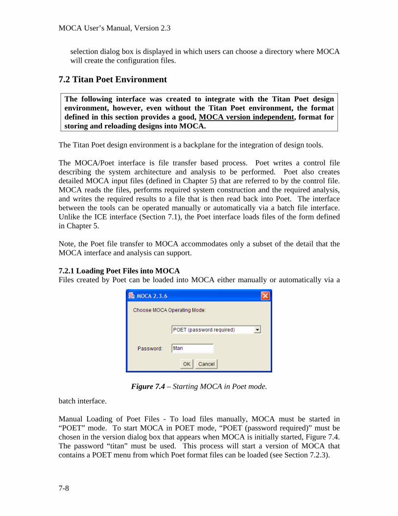
MOCA User’s Manual, Version 2.3
7-8
selection dialog box is displayed in which users can choose a directory where MOCA will create the configuration files.
7.2 Titan Poet Environment
The following interface was created to integrate with the Titan Poet design environment, however, even without the Titan Poet environment, the format defined in this section provides a good, MOCA version independent, format for storing and reloading designs into MOCA.
The Titan Poet design environment is a backplane for the integration of design tools. The MOCA/Poet interface is file transfer based process. Poet writes a control file describing the system architecture and analysis to be performed. Poet also creates detailed MOCA input files (defined in Chapter 5) that are referred to by the control file. MOCA reads the files, performs required system construction and the required analysis, and writes the required results to a file that is then read back into Poet. The interface between the tools can be operated manually or automatically via a batch file interface. Unlike the ICE interface (Section 7.1), the Poet interface loads files of the form defined in Chapter 5. Note, the Poet file transfer to MOCA accommodates only a subset of the detail that the MOCA interface and analysis can support. 7.2.1 Loading Poet Files into MOCA Files created by Poet can be loaded into MOCA either manually or automatically via a
batch interface. Manual Loading of Poet Files - To load files manually, MOCA must be started in “POET” mode. To start MOCA in POET mode, “POET (password required)” must be chosen in the version dialog box that appears when MOCA is initially started, Figure 7.4. The password “titan” must be used. This process will start a version of MOCA that contains a POET menu from which Poet format files can be loaded (see Section 7.2.3).
Figure 7.4 – Starting MOCA in Poet mode.

Chapter 7 – Integration with Other Tools
7-9
Automatic Loading of Poet Files – Poet files can also be loaded into MOCA via a batch interface that has the following syntax: [executable] POET [file] [graphic] where
[executable] = full path to the MOCA executable (should end with “analyzer.exe”) [file] = full path to the Poet input file to be loaded [graphic] = (OPTIONAL) full path to the MOCA title screen graphic (should end with “MOCA.gif”, this file is located in the “analyzer directory of the MOCA release). If this command is omitted, MOCA will start up and operate correctly, but the graphic that appears on the start up screen (Figure 3.2) will not appear.
If the above command is issued, MOCA will start up and load the designated file. MOCA will then perform the actions defined in the file and (optionally) shut down. 7.2.2 Poet File Format and Reference The Poet file is a text file containing variable names and values. The file has the following general structure: start_control_data
…[control variables defined here] end_control_data start_header
…[header variables defined here] end_header start_system_data
…[system variables defined here] start_board_data
…[board variables defined here] end_board_data start_board_data
…[board variables defined here] end_board_data
end_system_data Control Data (Variables) File Input Line and Data
Type Explanation Default
output_file = "<string>" Name of the file that MOCA should write output results into.
None
output_directory = "<string>" Full path to the directory which MOCA should write output results into (does not include the file name).
None
working_directory = "<string>" Full path to the working directory (does not include the file name). A working directory is assumed if the production events are loaded from a file.
None
load_configuration_path = "<string>"
*Path to MOCA configuration file to be loaded None
load_configuration_file = "<string>"
*Name of MOCA configuration file to be loaded None
Any number of boards can be included

MOCA User’s Manual, Version 2.3
7-10
price_file = "<string>" Name of the file that the Price model is stored in. None price_path = "<string>" Full path to the Price executable. None run_option = <integer> 0 – start MOCA but don't run MOCA
1 - start MOCA, run MOCA without Price 2 - start MOCA, run MOCA with Price 3 - start MOCA, run MOCA without Price and delete MOCA when done (hide all windows during execution if started from the command line) 4 - start MOCA, run MOCA with Price and delete MOCA when done (hide all windows during execution if started from the command line) run_options 3 and 4 include a 2 second MOCA window flash
0
combine_reorders = “<string>” *If “True” than reorders are combined; if “False” they are not. This entry appears in, Setup->Solution Control, Combine Reorders
“False”
budgeting = “<string>” *If “True” than the budgeting period is used; if “False” it is not. This entry appears in, Setup->Solution Control, Budgeting Period
“False”
number_of_refreshes = <int> *Number of refreshes per plan analyzed. This entry appears in, Setup->Solution Control, System With:
1
*Optional input Header Data (Variables) File Input Line and Data
Type Explanation Default
date = "<string>" *Used in header of MOCA output report only None author = "<string>" *Used in header of MOCA output report only None title = "<string>" *Used in header of MOCA output report only None info = “<string>” *Used in header of MOCA output report only None *Optional input System Data (Variables) File Input Line and Data
Type Explanation Default
system_name = "<string>" *Used in header of MOCA output report only None system_function = "<string>" *Used in header of MOCA output report only None number_boards = <integer> Total number of unique boards that will be defined in
the system (maximum = 50) None
hierarchical_name1 = "<string>" *Name used in labeling allocation table interface None hierarchical_name2 = "<string>" *Name used in labeling allocation table interface None hierarchical_name3 = "<string>" *Name used in labeling allocation table interface None avg_op_hours = <real> Average number of operational hours per year for the
system (only used if spares_in = “False”) 0.0 (no spares will be added)
base_year = <real> Analysis start date = base_year + EMD_period_start (July 1, 2003 = 2003.5). base_year also becomes the Discount Base Year and the Combine reorders start date.
0.0
EMD_period_start = <real> EMD_period_end = <real>
Design period start and end dates. The date should be in years after the base date. For example, if the base date is 2003.5 and the O&S period ends on January 1, 2021, the entry would be 17.5.
0
prod_period_start = <real> Production period start and end dates. The date 0

Chapter 7 – Integration with Other Tools
7-11
prod_period_end = <real> should be in years after the base date. For example, if the base date is 2003.5 and the O&S period ends on January 1, 2021, the entry would be 17.5.
OS_period_start = <real> OS_period_end = <real>
Operation and support period start date. The date should be in years after the base date. For example, if the base date is 2003.5 and the O&S period ends on January 1, 2021, the entry would be 17.5.
An end date of 0.0 (makes the end of O&S the same as the analysis start date)
prod_file_name = “<string>” The name of a production event file (see Section 5.4 for format). This file is assumed to be in the working_directory defined in the Control Data section. Loading this file takes the place of production_dates, production_quantity, and production_type. Up to 20 separate production files can be loaded (they will be concatenated together).
None
production_dates = <real>,<real>,…
List of dates separated by commas. The dates should be in years after the base date. For example, if the base date is 2003.5 and 350 units are to be produced by the end of 2005, the entry would be 1.5.
None
production_quantity = <real>,<real>,…
System production quantities corresponding to the dates above. There must be exactly one entry in the list for each date.
None
production_type = <int> 0 = Prototype, 1 = Reorder 1 redesign_cost_sys = <real> *Fixed cost of a redesign when the Price tool is not
used for redesign costing. This entry appears in the Redesign Fixed Cost field in the Design Selection Dialog box (Inputs->Design Selection) when the Price tool is not used for redesign costing.
0.0
redesign_cost_board = <real> *Fixed cost of a redesign per board affected when the Price tool is not used for redesign costing. This entry appears in the Redesign Cost/Board affected field in the Design Selection Dialog box (Inputs->Design Selection) when the Price tool is not used for redesign costing.
0.0
redesign_cost_component = <real>
*Fixed cost of a redesign per component affected when the Price tool is not used for redesign costing. This entry appears in the Redesign Cost/Component affected field in the Design Selection Dialog box (Inputs->Design Selection) when the Price tool is not used for redesign costing.
0.0
SubsystemQualificationCost = <real>
*Full re-qualification cost of the design this board is part of. This entry appears in the Re-Qualification cost field in the Design Selection Dialog box (Inputs->Design Selection).
0.0
NonCriticalPartThreshold = <integer>
Number of non-critical part changes that cause a full re-qualification to be performed at a design refresh.
0 (full re-qualification performed at every design refresh)
StorageHandlingFrac = <real> *Fraction of the part price charged per year for storage and handling (will be used for every part). Relevant to lifetime and last time buys. This entry appears for in the mitigation details for specific parts,
0.05 (5%)

MOCA User’s Manual, Version 2.3
7-12
Inputs->Components Definition, Set Mitigation, Simple Choice, <Go>.
MitigationFactor = <real> *Mitigation factor for a part. Will be used for every part – overrides all other entries of mitigation factor. This entry appears for in the mitigation details for specific parts, Inputs->Components Definition, Set Mitigation, Simple Choice, <Go>.
Taken from part-specific entries if not provided
budgeting_period = <real> *Budgeting period in years. This entry appears in, Setup->System Setup, Budgeting Period, <Set>.
1.0
combine_prod_years = <real> *Combine reorders in years. This entry appears in, Setup->System Setup, Combine reorders (yrs)
1.0
look_ahead_years = <real> *Redesign look ahead time in years. This entry appears in, Setup->System Setup, Redesign look ahead time (yrs)
0.0
time_to_refresh_years = <real> *Duration of the refresh in years. This entry appears in, Setup->System Setup, Duration of refresh (yrs)
0.0
discount_rate = <real> *Discount rate as a fraction/yr. This entry appears in, Setup->System Setup, Discount Rate (%/yr) as a percentage.
0.0
spares_in = "<string>" *True – spares are automatically computed by MOCA and added to the production scheduled False – MOCA will not automatically compute additional spares
False
*Optional input Board Data (Variables) File Input Line and Data
Type Explanation Default
parent = “<string>” Name of the board that this board is inside of, i.e., name of this boards parent. Parents must appear before children in the file.
“None”, board will be placed at the top-most level in the hierarchy
path = "<string>" Full path name to the board file. Does not include name of board file.
None
file = "<string>" Board file name. None name = “<string>” Board name. quantity = <integer> Number of instances of the board in the system or
parent. Note, the number of boards in a system defined in a loaded board file overrides this parameter.
1
replace_fraction = <real> Fraction of failed boards that are replaced with new boards (as opposed to repaired). Must be between 0.0 and 1.0, inclusive.
0.0 (no spares will be added)
base_date = <real> Analysis start date for this board (July 1, 2003 = 2003.5)
0
life_code_base_date = <real> If lifecodes are included in the board input files, MOCA requires a base data for the lifecodes (July 1, 2003 = 2003.5). This is the factor B defined in Section 4.1, which represents the date the lifecodes were generated.
initial production date
qstar = "<string>" *True – the file being loaded was generated by Q-Star
False – the board file

Chapter 7 – Integration with Other Tools
7-13
being loaded is in the MOCA format (Chapter 5)
qstar_name_option = "<string>" *Q-Star Name Options - Which column of the Q-Star report you wish to use as the unique part identifier “Part Number” in MOCA – allowed choices are: “Cust ref”, “Input Part No.”, ” In House PN”, or “Input Mfr PNo”. Ignored if qstar=”False”
None
qstar_tf_base_year = <real> *Q-Star Base Year - The date that the Q-Star file was generated. Ignored if qstar=”False”
0.0
board_cost = <real> *Initial manufacturing production cost of a single instance of the board. This entry appears in the Total Cost field on the Board Properties dialog box (Inputs->Board Definition->Define Properties) when “System” level qualification is used. Ignored if qstar=”False”
0.0
board_reliability = <real> *The board reliability measured in system operational hours. This entry appears in the Reliability (operational hours) field on the Board Properties dialog box (Inputs->Board Definition->Define Properties) and is interpreted as an MTBF. Only used if spares_in = “False”.
0.0
*Optional input Notes:
1) Only qualification at the system level is supported in this interface 2) Any number of levels of hierarchy are supported in this interface 3) Parents must be defined in the file prior to boards that are inside of them 4) Any number of boards can be included within the system, however, different
boards must be named uniquely 5) Extra properties can be included but will be ignored 6) If properties are included more than once, the last occurrence takes precedence 7) If duplicate component names are encountered during file loading, the last version
of the component encountered during loading overwrites all other components with the same name
8) In MOCA Version 2.1, the last base_date appearing in the file (within a board) is used as the analysis start date.
7.2.3 The POET Menu Poet generated files can be manipulated manually through the MOCA interface. When a Poet version of MOCA is started (Figure 7.4), a POET menu appears on the MOCA interface, Figure 7.5. The POET menu options are the following:
Import from POET… - Creates a file selection dialog box that allows Poet generated text files to be selected and loaded into MOCA. Note, run options that may be defined in the loaded file are interpreted as documented in the System Data table in Section 7.2.2.

MOCA User’s Manual, Version 2.3
7-14
Export to POET… - Not implemented in Version 2.3 of MOCA. 7.3 Price Systems H and HL Tools MOCA and Price exchange information using a DLL that should be installed when MOCA is installed (see Section 2.2). In order to use Price during a MOCA analysis uses the following steps:
1) Go to Setup->Solution Control and set the “Use Price for Redesign Costing” input to “On”.
2) The Price tools can be started by selecting Setup->Invoke Price Tool. A file browser dialog box will appear.
3) Navigate to the Price file that you wish to load (the one that corresponds to the design you have loaded into MOCA). The Price file corresponding to the example case introduced in Chapter 3 can be found in: MOCA_2.3/current_moca_6/data/MTC and is named “good MTC 3 board.hpr”. This file is shown in Figure 7.6.
4) After the file is selected and <Open> is pressed in the file browser, the Price software (assuming it is loaded on your system) will start-up by opening a Price Estimating Suite window as shown in Figure 7.7.
If a MOCA analysis is run and Price analysis is designated, but the Price tools are not invoked (step 2 above is not performed), the Warning message shown in Figure 7.8 will appear. Pressing <OK> will lead you through steps 3 and 4 above.
Figure 7.5 – MOCA interface with POET menu shown.

Chapter 7 – Integration with Other Tools
7-15
7.4 Q-Star Integration Q-Star is a commercial tool from QTEC (QinetiQ Technology Extension Corporation) that, among other things, generates obsolescence risks for electronic parts bills of materials (BOMs). MOCA reads Q-Star generated reports and assigns obsolescence date and lifetime length data to existing parts and/or new parts defined in the Q-Star report.
Figure 7.6 – File browser for locating Price data file.
Figure 7.7 – Price Estimating Suite window (example from Chapter 3 shown). The smaller window in the lower right is associated with MOCA’s connection to the Price
tool and will appear only when the analysis is executing – users do not need to interact with this window.

MOCA User’s Manual, Version 2.3
7-16
7.4.1 Q-Star Reports MOCA will load Q-Star generated reports that are saved in comma delimited format (.csv). Comma delimited format files can be created by spreadsheet programs such as Microsoft Excel using the “Save As…” command. A portion of a Q-Star output report is shown in Figure 7.9. The following columns of data are relevant to MOCA:
Cust ref = a customer reference number or name, one option for unique identifier assigned to the part within MOCA
Input Part No. = a part number or name, the other option for unique identifier assigned to the part within MOCA
Qty = number of instances of the part in the system LCC = lifecode (ranges from 0 to 5, 5 indicating that the part is
obsolete as of the date the report was generated). The lifecode represents the lifecycle phase a part is in.
YTEOL = years to end of life. Number of years past the date the report was generated that the part is expected to become obsolete.
Figure 7.8 – Warning message if Price Tools are not invoked.
Figure 7.9 – Example Q-Star output report.

Chapter 7 – Integration with Other Tools
7-17
Other data is contained within the Q-Star report, but it is not relevant to MOCA at this time. 7.4.2 Loading Q-Star Reports into MOCA To load Q-Star reports into MOCA, follow the steps below:
1) Select the “Load QStar File (.csv)” command from the File menu in the MOCA interface (select File->Load QStar File (.csv)), see Figure 7.10. A Q-Star Options dialog window will appear (see Figure 7.11).
2) The dialog box in Figure 3 will appear. Two pieces of information are needed in order to interpret the information contained in the Q-Star file:
a. Q-Star Name Options - Which column of the report you wish to use as the unique part identifier “Part Number” in MOCA – users can choose from columns named: “Cust ref”, “Input Part No.”, ” In House PN”, or “Input Mfr PNo”. Important note: if a column name is chosen that does not exist in the Q-Star file being loaded, an error will occur and the file will not be loaded.
b. Q-Star Base Year - The date that the Q-Star file was generated. This is the critical to determining the obsolescence dates from the Q-Star report data and is used as the value of the “base year”.
Pressing OK will record the data and continue the Q-Star file loading process (Figure 7.12), pressing Cancel will abort the Q-Star loading process.
Figure 7.10 – Q-Star file load menu item.

MOCA User’s Manual, Version 2.3
7-18
3) Navigate to the desired Q-Star file and select it from the file browser and press the <Open>.
At this point the Q-Star report will be loaded into MOCA subject to the following assumptions:
• When loading Q-Star report into MOCA, if duplicate part identifiers are encountered (either associated with existing components that were present before the Q-Star report was loaded, or appearing multiple times in the Q-Star report) an Action Window containing the warning message will appear (see Figure 3.6). The functions of the various buttons are described in Table 3.1.
Figure 7.11 – Q-Star report supplementary information dialog box.
Figure 7.12 – Loading the Q-Star report file.

Chapter 7 – Integration with Other Tools
7-19
• If no board has been defined in MOCA when the Q-Star report is loaded, MOCA will automatically create a new board and attach the specified number of instances of each part (Qty) to the board. If a board exists in MOCA when the Q-Star report is loaded, MOCA will create new parts in its global parts database, but not add them to any of the existing boards.
• If duplicate parts are encountered during the Q-Star report load and no board
is defined in MOCA prior to the Q-Star report load, the quantity of the duplicate part is added to the quantity of the existing part independent of whether the other part properties are replaced or not.
• The obsolescence date associated with the parts is determined by adding the base year, B (the date the Q-Star report was generated) to the years to end of life (YTEOL). The lifecode is used to determine the lifespan, L, of each component type. The lifespan is used when generating obsolescence dates for part replacements at design refreshes. See Section 5.3 of the MOCA User’s Guide V. 1.3 for an explanation of the calculation used.
• Parts that do not have YTEOL values are assigned obsolescence dates of 3100.0 (assumed to be effectively never become obsolete).
• The QStar file loading in MOCA requires that columns titled YTEOL and
LCC be present or an error is generated and the file is not loaded. The QStar file loading in MOCA also requires that the column titles appear on the second row of the spreadsheet and that the first row be non-blank. Both of these restrictions have been lifted.

Blank Page

Appendix A - Definitions
A-1
Appendix A - Definitions Aftermarket Source - A source of identical parts from a supplier who is not the original manufacturer of the part. Alternate Part - A replacement part with similar form fit and function that is equal to or better than the part it is replacing. Best Solution - Best solution, in the context of MOCA, refers to the lowest value of the quantity that is used to approximate the life cycle cost of the system. There are various quantities (called state metrics) in MOCA that can be chosen to pick the so-called best solution, e.g., mean life cycle cost, standard deviation of the life cycle cost, etc. The main criterion, which has been successfully used to compare various design refresh scenarios in MOCA, is mean life cycle cost of the system. The lower the mean cost, the better the solution. However, in cases where there exists multiple design refresh schedules with the same life cycle cost, then MOCA is not able to differentiate between the two scenarios. In that event, the case with the smallest number of design refreshes and earlier design refreshes is chosen to be the best case. Component - Used interchangeably with “part” in MOCA. Describes the lowest level of physical entity used in MOCA. Usually represents an electronic chip or discrete device. Design Refresh - A design refresh in the context of MOCA addresses product design. It is any activity that involves bringing about changes in the design of a product to incorporate one or more of the following:
• New or improved functionality • Mitigation of part obsolescence and other related issues • Reliability improvement of the system • Maintainable and repairable improvement • Incorporate new technology/innovations • Aesthetic improvement of product • Ease of use or more user-friendly • Change in documentation/engineering drawings
Important note, MOCA considers any change to the design (no matter how minor) to be a design refresh. For example, a part substitution that does not require any re-qualification would be considered a design refresh by MOCA. As a result, some design refreshes are very low cost.
Design Refresh Cost - Non-recurring cost incurred to carry out a design refresh from design conception through all actual design processes and simulations up to final documentation changed. Design Refresh Date - The design refresh date refers to the completion of all the design refresh activities carried out on the product.

MOCA User’s Manual, Version 2.3
A-2
Design Refresh Plan - A group of one or more design refreshes occurring during the product’s life (design, production, and sustainment). Emulation - A replacement part with the same form, fit, and function that was manufactured with a newer technology, but intended to be a drop in replacement for the part of interest. Existing Stock - Parts stock that is in storage awaiting use in product. When used as a obsolescence mitigation approach, existing stock is assumed to carry no recurring or non-recurring cost penalty. Failure Free Operating Period (FFOP) - The period of time (or appropriate units) during which no failures, resulting in a loss of system functionality, occur. Fielded Units - The systems that have been previously deployed to the field and are currently being supported. Last Time (Lasttime buy) Buy - Purchasing a sufficient quantity of identical parts to satisfy the product’s needs until the next design refresh. Also called a bridge buy. Lifecode – TACTech risk index indicating the life cycle stage of an electronic part. Generally, 1 = introduction, 2 = growth, 3 = maturity, 4 = saturation, 5 = decline, and 6 = phase-out. Life Cycle Cost - The design cost, production cost, operation cost, support cost and disposal cost together make up the life cycle cost of the system. In the context of MOCA, original design cost and disposal costs are not included in the life cycle cost assessment. However, any design changes after the original design, i.e., non-recurring design costs associated with a design refresh of the system and it’s cost impact on the life cycle cost of the system are included. Lifetime Buy - Purchasing a sufficient quantity of identical parts to satisfy the entire product’s lifetime needs. Look-Ahead Time - Look-ahead time means that whenever a design refresh takes place, MOCA “looks-ahead” for forecasted part obsolescence issues and pro-actively removes those part obsolescence problems at the current design refresh opportunity. By having a long design refresh look-ahead time the number of design refreshes might be reduced. On the other hand, by design refreshing parts that are not yet obsolete there is a risk of incurring extra cost for no improvement, i.e., there is a possibility that the obsolete part that was proactively design refreshed is never required in the future. Mean Time Between Failure (MTBF) - The average amount of time that passes between random failures in a system.

Appendix A - Definitions
A-3
Mitigation - A process or mechanism used to manage an obsolescence problem, e.g., lifetime buy, last time buy, aftermarket source, substitute part, reclaim, or emulation. Obsolescence - A part becomes obsolete when it is no longer manufactured, either because demand has dropped to low enough levels that it is not practical for manufacturers to continue to make it, or because the materials or technologies necessary to produce it are no longer available. Operation and Support Cost - This cost is the cost incurred to maintain the system through it’s life time and keep it in a functioning state. Original Manufacturer or Original Equipment Manufacturer (OEM) - In the context of MOCA, the manufacturer from which the part was procured for the current design of a product is defined as original manufacturer. Part - Used interchangeably with “component” in MOCA. Describes the lowest level of physical entity used in MOCA. Usually represents an electronic chip or discrete device. Part Obsolescence Date - The obsolescence date of a part in MOCA, is the date after which the part is no longer available from the original manufacturer (from which the part was procured for the current design). Product Life Cycle - Seven common life cycle stages: introduction, growth, maturity, saturation, decline, phase-out, and discontinuance make up a product’s life cycle. Production Cost - This is the recurring cost incurred by the manufacturer to produce the system after it has been designed and developed. From consumer’s point of view it is the procurement cost to acquire the system. Qualification and Re-qualification - The process of qualification is defined as the ability of the nominal design and manufacturing specifications of the product to meet the customer's needs. Qualification is performed during initial product development and may be performed after any design or manufacturing changes in an existing product (re-qualification). Reclaim - Use of identical parts that have been salvaged from other products. Refresh, Redesign and Insertion – Refresh and redesign are used interchangeably in MOCA and its documentation. However, in actuality the definitions can be distinguished: Technology Refresh is used as a reference to system changes that “Have To Be Done” in order for the system functionality to remain viable. Redesign and Technology Insertion is used to identity the “Want To Be Done” system changes, which

MOCA User’s Manual, Version 2.3
A-4
include both the new technologies to accommodate system functional growth and new technologies to replace and better the existing functionality of the system.1 Reorder - With each additional order, a new quantity of systems comes into existence. Each order has a unique start date for the new system’s maintenance events or repair events. A reorder can occur either due to maintenance requirements or due to production, which may be spread over the lifetime of the product. The production can be for units, which were planned initially at the design stage, or addition orders during the product’s field support life (spares). Reorder Date - Reorder date represents the start of processing of an order request or start of a planned production. Retrofit – Replacement of fielded product in order to update or upgrade. The product replaced has not necessarily failed. Replenishment spares can be used to retrofit (initial spares cannot be used to retrofit). State Metric(s) - There are various metrics by which best solutions can be determined. Criteria could include lowest mean cost, lowest variance in cost, or earliest design refresh dates or combinations of these. Spares - Spare product is produced in anticipation of a future need for additional product either to replace failed product or to fulfill future additional product orders. Two types of spares are used in MOCA:
Initial Spares – Built along with the original production, then stored until needed. Used to replace failed product. Replenishment Spares – Built at a date later than the original production data either because initial spares were depleted or updated product is required for retrofitting fielded product.
Substitute Part - A replacement part with similar form fit and function that is inferior to the part it is replacing. Time Scale or Simulation Step - The smallest time period, i.e., hours or minutes or days, etc., used to specify the time-based events that occur in MOCA is defined as the time scale or simulation step.
1 T. E. Herald, “Technology Refreshment Strategy and Plan for Application in Military Systems – A “How-To Systems Development Process” and Linkage with CAIV,” Proc. National Aerospace and Electronics Conference (NAECON), pp. 729-736, October 2000.

Appendix B – MOCA Date Conversion
B-1
Appendix B – MOCA Date Conversion MOCA requires input dates for many different things including obsolescence and production events. MOCA requires that dates be entered as real numbers that have the following format: a.b where
a = the year, e.g., 2005 b = the fraction of one year corresponding to the calendar date.
Examples:
January 1, 2011 = 2011.0 July 1, 2008 = 2008.5 (July 1 is the 182 day of the year)) September 23, 2009 = 2009.73
(September 23 is the 266th day of the year, b = 266/365 = 0.73)

Blank Page

Appendix C – Obsolescence Mitigation Factor Calculation
C-1
Appendix C – Obsolescence Mitigation Factor Calculation If Lifetime or Lasttime buy are chosen as the mitigation approach in the Simple choice obsolescence mitigation model (see Section 4.1.1), the mitigation factor can be computed using the model described in this appendix. Figure C.1 shows the dialog box associated with the Simple choice model with Lifetime buy chosen. C.1 Model Construction The original vendor, from whom parts were purchased for the current design, might offer the parts for last time buys or lifetime buys at a different price. The parts could also be discounted since the lifetime buys/last time buys are usually made in large quantities. Figure C.2 shows the assumed discounting curve for lifetime buys or last time buys used in MOCA. The discounting curve has an exponential section at the start and end with a bridging straight line in the middle. From the start until quantity Q0, P0 is the fixed discount rate. At Q0 the exponential shape of the curve starts. The end of the curve reaches up to a maximum percentage discount P3. This curve is based on a generalized curve representing quantity-based events. The curve is general enough that by varying the parameters P1, P2, P3, and Q1, the shape of the curve can be varied extensively.
Figure C.1 – Simple choice mitigation factor dialog box with Lifetime buy chosen.

MOCA User’s Manual, Version 2.3
C-2
Note: The parameters can be negative. A negative value of percentage discount rate implies increase in procurement cost where as a positive value of percentage discount rate implies decrease in procurement cost.
0
10
20
30
40
50
60
70
80
0 500 1000 1500 2000 2500 3000 3500
Quantity
% D
isco
unt
Qo
Po
P1
P2
P3
Q10
10
20
30
40
50
60
70
80
0 500 1000 1500 2000 2500 3000 3500
Quantity
% D
isco
unt
Qo
Po
P1
P2
P3
Q1
Figure C.2 - Discount curve for Lifetime buys and Lasttime buys.

Appendix D – Refresh Selection Algorithm
D-1
Appendix D – Refresh Selection Algorithm1
One of the key attributes of the MOCA methodology is its treatment of uncertainties. Obviously, much of the data that the method depends on to make design refresh decisions is highly uncertain. In order to solve the problem two types of uncertainties must be managed, 1) uncertainties in the inputs to the cost analysis, for example, the re-qualification cost associated with a particular type of qualification test; and 2) uncertainties in dates. The first type of uncertainty is handled through simple Monte Carlo modeling. The second type of uncertainty (dates) is more complex to accommodate. At the highest level in the solution, an algorithm that selects a candidate refresh plan is used. A candidate refresh plan consists of the quantity of design refreshes in the lifetime of the product and the dates of those refreshes relative to production events, Figure D.1. A production event is any event that results in the need to produce additional instances of the product, i.e., additional orders or spare replenishment necessary for sustainment. Once a candidate refresh plan is chosen, an actual sampling of dates for the production events is chosen (the date for each production event is input as a probability distribution). After the probability distributions for the dates are sampled, a sample refresh plan (with real dates) is available. The methodology then computes the life cycle cost of the candidate refresh plan for the sample. Using a basic Monte Carlo approach, the methodology repeats the process of sampling production dates and computing life cycle costs a statistically relevant number of times producing a histogram of the life cycle costs for the candidate refresh plan.
Another important aspect of the algorithm is the identification and use of a time step (budget period, Section 4.7). Unlike physical simulations, where the smaller the time step chosen for the simulation, the more accurate the answer; in this simulation, too small a time step may be just as inaccurate as too large a time step. The correct time step to use is one that corresponds to the OEMs procurement cycle, i.e., how quickly are part procurement decisions made, vendors approved, and procurements completed (parts in-house and ready for use in products) – normally, we assume times steps on the order of 1-2 quarters. In this methodology, for a given time step size, after the sampled candidate
1 P. Singh and P. Sandborn, "Obsolescence Driven Design Refresh Planning for Sustainment-Dominated Systems," The Engineering Economist, Vol. 51, No. 2, pp. 115-139, April-June 2006.
Production Date
Prob
abili
ty
Sample
Timeline
Design Refreshes
Production Events
Production Date
Prob
abili
ty
Sample
Timeline
Design Refreshes
Production Events
Figure D.1 - A candidate refresh plan in defined as one or more design refreshed
and their dates relative to production events.

MOCA User’s Manual, Version 2.3
D-2
refresh plan is determined, the resulting timeline is dropped onto a grid (Figure D.1) that corresponds to the time step (each date in the sample is moved to the closest point on the time step grid).

Appendix E – MOCA Input Requirements Summary
E-1
Appendix E – MOCA Input Requirements Summary There are five categories of inputs are necessary to populate the MOCA model. 1) Part inputs, which include part costs, part characterization data and obsolescence data. These inputs represent the overall part database from which parts can be selected for inclusion in boards. 2) Board inputs, which include: board cost, qualification, reliability, and the list of parts assigned to each board. In a broad sense, the board can be interpreted as any subsystem containing parts. 3) System inputs include dates for the beginning and end of the system’s life, cost factors for obsolescence mitigation approaches, and the cost of taking the system out of service for maintenance. 4) Qualification inputs. 5) Data uncertainties. In addition to these, solution control inputs are used to control various parameters required to compute the sustainment cost and plan the design refreshes.
1. Part a. Part Number or Name (some unique identifier) b. Part Price (what the OEM pays per instance of the part for the original part) c. Obsolescence Date (or alternatively a “life code” 1-5 indicating where in the life
cycle the part currently is), 1 = introduction, 2 = growth, 3 = mature, 4 = decline, 5 = discontinuance, 6 = obsolete -- this data can be optionally loaded for a report generated by a commercial tool.
d. Short-Term Obsolescence Management Strategy (what do you want to do between the obsolescence event and the next design refresh) – note this can be globally defaulted for the entire BOM – “Existing Stock”, Aftermarket Source”, “Emulation”, Lasttime buy, Lifetime buy, reclaim, alternative
e. Part category (type of part – Microprocessor, Transistor, Diode, Semiconductor, Custom, etc.)
f. (Complexity Level) – can be defaulted by the tool, used in synthesis of a part replacement
g. (Redesign Cost Multiplier) – can be defaulted by the tool, used in synthesis of a part replacement
2. Board a. Board Number or Name (some unique identifier) b. Parts List for the Board with:
i. number of instances of each part on the board ii. any specific qualification activities driven by the part (defaults to no
special qualification activities) c. Total Cost (board, assembly, parts, functional test – total recurring cost) d. Reliability in total operational hours (distribution too) – this can be MTBF for
FFOP (Failure Free Operating Period) – only required if MOCA has to compute sparing requirements
e. Fraction of failures that require replacement boards – fraction of the reliability field failures that can not (or will not) be repaired and require the manufacture of

MOCA User’s Manual, Version 2.3
E-2
a replacement board – used in spare replenishment calculation (0.0 – 1.0), 0 means that no spares are needed – everything is fixed, nothing replaced; 1 means that everything that fails is replaced – only required if MOCA has to compute sparing requirements
f. MOCA also has the ability to build up to a 6-level hierarchy (boards in board in boards, etc.). If a hierarchy is required, parent-child relationships must be defined.
3. System a. List of Boards in the System (with number of instances of each board) b. Quantity of Systems Manufactured by some time unit (month, year, etc.) c. Are Spares Included in the Quantity Data – MOCA can automatically compute
spare replenishments if necessary d. Analysis Start Date (could be start of design process) e. Field Start Date (usually coincides with first production) f. End of Product Support Date g. Average Operational Hours Per Year – only required if MOCA has to compute
sparing requirements h. Any known system events:
1. Reorder Dates (additional orders) 2. Fixed Redesign Dates (if any) 3. Any redesign “blackout” dates (time periods when you can not do
a redesign) – driven by budget constraints or logistical constraints (military)
i. Cost Modeling Data (only needed if Price H/HL tools are not to be used): 1. Redesign fixed cost (charged for every redesign activity) 2. Redesign cost per board affected (base charge for every board
touched at a redesign) 3. Redesign cost per component affected (base charge for every part
touched at a redesign)
4. Qualification Data
a. Total (full) re-qualification cost
b. List of qualification levels (some unique name given to each name can not be “None” or “Full”) + cost of each level is performed independently
c. Number of non-critical component changes that trigger a full re-qualification
d. Qualification (and the details above) can be performed at the system level or at the specific board level, i.e., there could be unique costs and qualification levels for each board, or costs and qualification levels could be applied to the whole system.
5. Uncertainties – optional (MOCA can default these)

Appendix E – MOCA Input Requirements Summary
E-3
a. A probability distribution shape (uniform, normal, lognormal, triangular, or none) can be defined for each data input. MOCA defaults to “None” – no distribution
b. If a distribution is assigned to an input, the relevant properties of the distribution must be provided, i.e., mean or most likely value, standard deviation, or the low and high points.

Blank Page

Appendix F – Description of MOCA “Development” Mode
F-1
Appendix F – Description of MOCA “Development” Mode The MOCA “Development” mode is a repository for MOCA functionality that is either under development (incomplete in some cases), not fully documented, or not robust enough for the default version of the MOCA tool. The Development mode contains all the same functionality as the default mode, plus additional functionality. The following development mode MOCA functionality is discussed in this Appendix:
Technology insertion version of MOCA NSWC Horizon integration to MOCA Synthesizing floating obsolescence dates Weeding out unused boards Obsolescence case resolution costs Part type controllable obsolescence dates Accumulating (and plotting) obsolescence events
If you wish to use the specific functionality listed above, you are encourage to contact CALCE for help.
The Development version of MOCA can be entered into either by starting MOCA in the development mode with password “umd” (Figure F.1), or by switching to the Development mode within MOCA (File->Change MOCA Operating Mode->Development, password = “umd”). F.1 Technology Insertion MOCA The Default mode of MOCA described in this user’s guide targets technology sustainment, i.e., maintaining a static functional capability, but what about evolving requirements and technologies? An extension to this methodology that expands the design refresh value proposition to include more than obsolescence effects has been developed. This extension enables optimum technology insertion into systems based on a value proposition that includes performance, reliability, cost and sustainability.
Figure F.1 – Starting MOCA in the Development mode.

MOCA User’s Manual, Version 2.3
F-2
The previously discussed MOCA methodology (Chapter 1) uses a very simple rule to determine the parts addressed at each candidate refresh: replace all parts that have become obsolete since the last refresh and all parts that are forecasted to become obsolete within a user defined period of time (“look-ahead” time) measured from the start of the candidate refresh activity. In reality, the decisions that govern whether a part is changed (replaced or upgraded) or not changed at a design refresh depend on the obsolescence attributes of the specific part and on the "utility" to the system realized by changing the part (cost, performance, reliability, and future sustainability). The approach followed in the technology insertion version of MOCA is to use Bayesian Belief Networks (BBNs), to decide design refresh content for candidate design refresh dates generated by MOCA. BBNs are applicable for reasoning about beliefs under conditions of uncertainty and using disparate sources of evidence (diverse data sources that include subjective beliefs and data that is highly uncertain). A second motivation for using BBNs is that sharing an understanding among many heterogeneous stakeholders (procurement, design, manufacturing, etc.) using both qualitative and explicit data is a necessity when managing the lifecycle of sustainment-dominated products. Decision analysis has the capability to consider all the decision affecting variables at the same time in the model, e.g., availability of a new part to replace the old part, available stock of the old part, performance and reliability changes due to the part changes, re-qualification that may be triggered by part changes, etc. Figure F.2 shows the MOCA analysis architecture and indicates where the elements of the decision model fits within it. This approach ensures that we consider both dimensions of optimization, i.e., date of the design refresh
Production Plan
Product Design and Planning
Forecast Obsolescence
- Technology/Part Selections
- Production schedule
Usage scenarioReliability
- Spare requirements
- Production plan(quantity and schedule)
Choose Refresh Candidates
- Viable Refresh Dates
Select a Candidate Refresh Plan
- Plan (multiple refresh dates)
Determine Highest Value Actions to Take at each Design Refresh
- Design Changes
- Obsolescence Dates
Budget Constraints
Modify the Design
Life Cycle Cost Analysis
Next design refresh in the plan
Synthesize New Technology/Parts
Determine value of the refresh plan
Nex
t pla
n
- Non-recurring redesign costs- Re-qualification costs- Software re-hosting costs- Recurring cost of obsolescence mitigation
- Production plan
VALUE
Construction of BBN – generation of nodes, node links, and
population of probability tables
BBN Update –populate updated probability tables
Determine design refresh content
using BBN
Figure F.2 – BBN decision model within the MOCA architecture.

Appendix F – Description of MOCA “Development” Mode
F-3
along with what is changed at the design refresh. The “technology sustainment” version of MOCA decides to design refresh parts at a design refresh simply because they are obsolete (not an unrealistic situation for avionics and military systems). However, for some of the parts, continuation of mitigation approaches (e.g., purchase from an aftermarket source or use on an emulated part) might have been preferable to replacement at the refresh due to the cost, reliability, and/or performance penalties that may be associated with the replacement. For this kind of situation a BBN model helps prevent “over design refreshing” of the system. Another possibility is that replacement of a non-obsolete part might be preferred because it is less expensive, more reliable, or improves the performance sufficiently to justify the cost of replacing it. F.1.1 Using the Technology Insertion Version of MOCA The Technology Insertion version of MOCA constructs Bayesian Belief Networks for selected parts. The parts that are included in the BBNs can be selected by going to the Parts Dialog box (Inputs->Components Definition) and switching the “Use BBN” to “true” for the parts you wish to include (it will initially be defaulted to “false” for all the components). Note, you must click somewhere else in the table after you make your last change in the “Use BBN” column in order for your last change to be recognized by MOCA. The probability tables that reside within the nodes of the BBN are automatically generated by MOCA. The data used to generate the probability tables comes from the inputs associated with the default version of MOCA and some comes from inputs that are specific to the Development version of MOCA. The Development version specific inputs are found at Inputs->Modify … To run the analysis with the BBNs included you must have the Hugin Expert tool (not included within the MOCA release). To run the analysis use the Compute/Results->Run …. with BBN commands. As a byproduct of the analysis, MOCA will generate a file containing the BBN built for the chosen component set. The file is named …_huginNet.hkb and is located in the current directory. The file can be viewed and manipulated outside of MOCA using the Hugin Expert tool (note, you need not view or manipulate this file outside of MOCA in order to perform the MOCA analysis). The architecture of the BBN created by MOCA can be controlled by checking or unchecking the Setup->Split BBN menu item. By default, Split BBN will be checked causing the BBN constructed by MOCA to be d-seperated, which greatly decreases the execution time in MOCA, but produces networks that are more difficult to understand and manipulate outside of MOCA. If the Split BBN is unchecked, the BBNs generated by MOCA are easier to view and understand outside of MOCA.

MOCA User’s Manual, Version 2.3
F-4
F.2 NSWC Horizon Integration The Development mode of MOCA has the ability to integrate its analysis with the Horizon tool suite from NSWC Crane. The Horizon Solution Suite Technology Refresh Cost Model (NAVSURFWARCENDIV Crane) is an engineering-based model used to estimate the costs associated with a technology refresh of systems.1 The model allows NAVSURFWARCENDIV Crane to join the functions of analyzing and identifying critical obsolescence issues in military systems. The model also forecasts future costs of refreshing equipment and determines feasible schedules for technology refresh. This enables our customers to proactively manage and budget for essential technology upgrades to their systems. The integration requires that the Horizon tool be present on the system where MOCA is being run. The key MOCA commands available for this integration including:
Inputs->Create Horizon Hierarchy = pops up a file browser that allows loading of a scenario file (created by Horizon to provide MOCA with hierarchy or framework for the analysis). Inputs->Populate BBN (Horizon) = works iteratively with Horizon to determine the values for populating the probability tables in MOCA generated BBNs (only relevant if analysis with BBNs is being used in conjunction with the Horizon tool). Setup->Horizon Cost Structure Setup = displays the Horizon cost breakdown and allows MOCA users to choose the costs returned from Horizon that are included in the MOCA analysis. Setup->Solution Control, Cost Analysis: Horizon = this must be chosen in order to run the analysis using the Horizon tool for costing.
F.3 Synthesizing Floating Obsolescence Dates If the “Obs date” of a part being loaded into MOCA from a .csv file (see Chapter 5) is given the value: “Floating obs date” the obsolescence date of the part is set to “NA” by default when it is loaded into MOCA. However, the part is a candidate for obsolescence date synthesis. In the development mode, users can selection Setup->Synthesize Obs Dates. When this selection is made, the entire parts list is searched. For each part with a “Floating obs date,” the date of first use of the part is found (by searching through all the production events associated with building product and finding the earliest date on which the part is required). The date of first use is used along with the part’s procurement 1 M. Chestnutwood and R. Levin, “Technology Assessment and Management Methodology – An Approach to Legacy System Sustainment Dynamics,” in Proceedings Navy Logistics Conference, October 19-21, 1998.

Appendix F – Description of MOCA “Development” Mode
F-5
lifetime and the “Lifecode of Synthesized Parts” to synthesize an obsolescence date for the part. If the part is never used, its obsolescence date remains “NA”. The procurement lifetime for the part is taken from Column 9 of the board .csv file if provided. If not provided, the procurement lifetime provided for the part type from the Part Synthesis Solution Control dialog box is used. Both “System” and specific board production events are searched (component production events are not searched). Limitations: Only the first level of the board hierarchy is searched for the part, i.e., if more levels of hierarchy are present, the search may fail. F.4 Weeding Out Unused Boards In Development mode, a button called <Remove Unused Boards> appears in the Boards Dialog box (Figure 4.9). This button will delete all boards from MOCA that do not appear in at least one Reorder, Spare Replenish or Prototype production event. This may be important to the analysis since MOCA refreshes all boards (whether used or not) that an obsolete part appears on at each refresh opportunity. There is no warning or undo for this command. Limitations: Only the first level of the board hierarchy is searched for the part, i.e., if more levels of hierarchy are present, the search may fail.
F.5 Obsolescence Case Resolution Costs In Development mode, part type specific obsolescence case resolution costs can be defined. The case resolution cost will be charged exactly one time for the part no matter how many instances of the part there are or how many different places within the system it appears. The part type specific case resolution cost (Case Res Cost) from the Part Synthesis Solution Control dialog box (Figure F.3) is used if it is greater than 0, otherwise, the Redesign Cost/Component Affected (Section 4.3) is charged when a design refresh occurs. This cost is charge exactly one time. All the type-specific case resolution costs default to 0. Note, MOCA does not have to be in development mode for this functionality to work, however, MOCA must be in development mode in order to set the Case Res Cost column values in the Part Synthesis Solution Control dialog box. F.6 Part Type Controllable Obsolescence Dates In Development mode, the Poet keyword “TypeSpecificObsDates” can be used to optionally control setting the obsolescence dates for parts. If TypeSpecificObsDates = True is included in the Poet file (in the System data section) than the obsolescence date is taken from the “Obs Date” column on the Part Synthesis Solution Control dialog box (Figure F.3) when the part is loaded. If TypeSpecificObsDates = False (default condition), the obsolescence date is taken from the loaded file. Note, MOCA does not have to be in development mode for this functionality to work, however, MOCA must be in development mode in order to set the Obs Date column values in the Part Synthesis Solution Control dialog box.

MOCA User’s Manual, Version 2.3
F-6
F.7 Accumulating Obsolescence Events The quantity of obsolescence events can be accumulated and plotted on the timeline for miscellaneous system management cases. Choosing Compute/Results->Accumulate Obsolescence Events displays the dialog box shown in Figure F.4. The buttons in the dialog box apply different scenarios to the loaded system and produces a count of the quantity of part-level obsolescence events occurring as a result. Figure F.5 shows example results for the example case discussed in Chapter 3. Note, the “Last run” option is not implemented in Version 2.3.
Figure F.3 – Part Synthesis Solution Control dialog box in development mode.

Appendix F – Description of MOCA “Development” Mode
F-7
Figure F.4 – Obsolescence Event Accumulation dialog box.
Figure F.5 – Example obsolescence accumulation results. Top = Design refresh at all obsolescence events; Bottom = Lifetime buy at all obsolescence events.

MOCA User’s Manual, Version 2.3
F-8
F.8 Miscellaneous Additional Menu Commands Some miscellaneous additional menu commands are documented in this section. Note, there are many more menu commands included in the Development mode than what is listed here. Setup-> Invoke Price Tool Invokes the Price tool. The Price tool has to be invoked when the user has chosen to use Price for redesign costing in the Solution Control dialog box. Note, when the user chooses to Compute/Results->Run Cost Analyzer or Compute/Results->Run Design Optimization (both are discussed later in this section), i.e., carry out the analysis, they will be prompted to start the Price tool if it has not been started using this command.