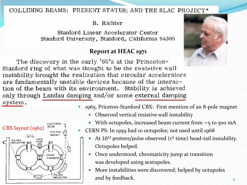
report at heac 1971 - cbp.lbl.govcbp.lbl.gov/seminar/archive/nagaitsev_07dec2010.pdf · report at...
TRANSCRIPT

2
Report at HEAC 1971
CBX layout (1962)
1965, Priceton-Stanford CBX: First mention of an 8-pole magnet
Observed vertical resistive wall instability
With octupoles, increased beam current from ~5 to 500 mA
CERN PS: In 1959 had 10 octupoles; not used until 1968
At 1012 protons/pulse observed (1st time) head-tail instability.
Octupoles helped.
Once understood, chromaticity jump at transition
was developed using sextupoles.
More instabilities were discovered; helped by octupoles
and by feedback.

3
How to make a high-intensity machine? (OR, how to make a high-intensity beam stable?)
1. Landau damping – the beam’s “immune system”. It is related to the spread of betatron oscillation frequencies. The larger the spread, the more stable the beam is against collective instabilities.
2. External damping (feed-back) system – presently the most commonly used mechanism to keep the beam stable.
• Can not be used for some instabilities (head-tail)
• Noise
• Difficult in linacs

4
Most accelerators rely on both
LHC
Has a transverse feedback system
Has 336 Landau Damping Octupoles
Provide tune spread of 0.001 at 1-sigma at injection
In all machines there is a trade-off between
Landau damping and dynamic aperture.
• …But it does not have to be.

5
Today’s talk will be about…
… How to improve beam’s immune system (Landau damping through betatron frequency spread) Tune spread not ~0.001 but 10-50%
What can be wrong with the immune system? The main feature of all present accelerators – particles have
nearly identical betatron frequencies (tunes) by design. This results in two problems: I. Single particle motion can be unstable due to resonant
perturbations (magnet imperfections and non-linear elements);
II. Landau damping of instabilities is suppressed because the frequency spread is small.

6
Courant-Snyder Invariant
Courant and Snyder found a conserved quantity:
yxz
zsKz
or
,0)("
Equation of motion for betatron oscillations
3
1)( where
sK -- auxiliary equation
22 )(
2
)(
)(2
1zsz
sz
sJ
yyxxyx JJJJH ),(
yx JJ , -- are Courant-Snyder integrals of motion
xx
J
H
yy
J
H
-- betatron frequencies

Linear function of actions: good or bad?
It is convenient (to have linear optics), easy to model, …but it is NOT good for stability.
We did not know (until now) how to make it any other way!
To create the tune spread, we add non-linear elements (octupoles) as best we can
Destroys integrability!
7
yyxxyx JJJJH ),(
octupole
Tune spread depends on a linear tune location 1-D system:
Theoretical max. spread is 0.125
2-D system: Max. spread < 0.05

8
First non-linear accelerator proposals (before KAM theory)
In a series of reports 1962-65 Yuri Orlov has proposed to use non-linear focusing as an alternative to strong (linear) focusing.
Final report (1965):

9
McMillan nonlinear optics
In 1967 E. McMillan published a paper
Final report in 1971. This is what later became known as the “McMillan mapping”:
)(1
1
iii
ii
xfxp
px
CBxAx
DxBxxf
2
2
)(
const 222222 DxppxCxppxBpAx
If A = B = 0 one obtains the Courant-Snyder invariant

10
McMillan 1D mapping
At small x:
Linear matrix: Bare tune:
At large x:
Linear matrix: Tune: 0.25
Thus, a tune spread of 50-100% is
possible!
CBxAx
DxBxxf
2
2
)(
xC
Dxf )(
C
D1
10
C
D
2acos
2
1
0)( xf
01
10
4 2 0 2 4
4
2
0
2
4
pn k
xn k
A=1, B = 0, C = 1, D = 2

11
What about 2D optics?
How to extend McMillan mapping into 2-D?
Danilov, Perevedentsev found two 2-D examples:
Round beam: xpy - ypx = const
1. Radial McMillan kick: r/(1 + r2) -- Can be realized with an “Electron lens” or in beam-beam head-on collisions
2. Radial McMillan kick: r/(1 - r2) -- Can be realized with solenoids (may be useful for linacs)
In general, the problem is that the Laplace equation couples x and y fields of the non-linear thin lens

12
1 octupole in a linear 2-D lattice
Typical phase space portrait:
1. Regular orbits at small amplitudes
2. Resonant islands + chaos at larger
amplitudes;
Are there “magic” nonlinearities that
create large spread and zero resonance
strength?
The answer is – yes
(we call them “integrable”)

Long-term stability The first paper on the subject was written by Nikolay Nekhoroshev in 1971
He proved that for sufficiently small ε
provided that H0(I) meets certain conditions know as steepness
Convex and quasi-convex functions H0(I) are the steepest
An example of a NON-STEEP function is a linear function
Another example of a NON-STEEP function is
13
2211210 ),( IIIIH
22
21210 ),( IIIIH

Non-linear Hamiltonians We were looking for (and found) non-linear 2-D steep
Hamiltonians that can be implemented in an accelerator
Other authors worked on this subject recently: J. Cary, W. Wan et al., S. Danilov, E. Perevedentsev
The problem in 2-D is that the fields of non-linear elements are coupled by the Laplace equation.
An example of a steep (convex) Hamiltonian is
but we DO NOT know how to implement it with magnetic fields…
14
0 ,),( 222
211210 IIIIH

What are we looking for?
We are looking for a 2-D integrable convex non-linear Hamiltonian,
-- convex curves
15
),(),( 21210 IIhIIH
constIIh ),( 21
I1
I2

16
Our approach See: Phys. Rev. ST Accel. Beams 13, 084002
Start with a round axially-symmetric LINEAR focusing lattice (FOFO) Add special non-linear potential V(x,y,s) such that
400
Sun Apr 25 20:48:31 2010 OptiM - MAIN: - C:\Documents and Settings\nsergei\My Documents\Papers\Invariants\Round
20
0
50
BE
TA
_X
&Y
[m]
DIS
P_X
&Y
[m]
BE TA_X BE TA_Y DIS P_X DIS P_Y
V(x,y,s) V(x,y,s) V(x,y,s) V(x,y,s) V(x,y,s)
0),(),,( yxVsyxV

17
Special time-dependent potential
Let’s consider a Hamiltonian
where V(x,y,s) satisfies the Laplace equation in 2d:
In normalized variables we will have:
),,(
2222
2222
syxVyx
sKpp
Hyx
)(,)(,)()(
22
2222
syxVyxpp
H NNNNyNxN
N
0),(),,( yxVsyxV
s
0)s(
d)(
ssWhere new “time” variable is
,)(2
)()(
,)(
s
zsspp
s
zz
N
N

Four main ideas 1. Chose the potential to be time-independent in new
variables
2. Element of periodicity
3. Find potentials U(x, y) with the second integral of motion
4. Convert Hamiltonian to action variables
and check it for steepness
),(
22
2222
NNNNyNxN
N yxUyxpp
H
sL
β(s)T insert
100
0100
001
0001
k
k 2
211
)(
Lk
sLskLs
18
),(),( 21210 IIhIIH

Integrable 2-D Hamiltonians Look for second integrals quadratic in momentum
All such potentials are separable in some variables (cartesian, polar, elliptic, parabolic)
First comprehensive study by Gaston Darboux (1901)
So, we are looking for integrable potentials such that
),(22
2222
yxUyxpp
Hyx
),(22 yxDCppBpApI yyxx
,
,2
,
2
22
axC
axyB
cayA
19
Second integral:

Darboux equation (1901) Let a ≠ 0 and c ≠ 0, then we will take a = 1
General solution
ξ : [1, ∞], η : [-1, 1], f and g arbitrary functions
033222 yxxyyyxx xUyUUcxyUUxy
22
)()(),(
gfyxU
c
ycxycx
c
ycxycx
2
22222
2222
20

The second integral The 2nd integral
Example:
22
222222 )()(
2,,,
gfcpcypxpppyxI xxyyx
22
2
1),( yxyxU
1
2)( 22
2
1 c
f 222
1 12
)( c
g
22222,,, xcpcypxpppyxI xxyyx
21

Laplace equation Now we look for potentials that also satisfy the Laplace
equation (in addition to the Darboux equation):
We found a family with 4 free parameters (b, c, d, t):
0 yyxx UU
acos1)(
acosh1)(2
2
2
2
tbg
tdf
22
)()(),(
gfyxU
22
The most interesting: d=0 and tb2
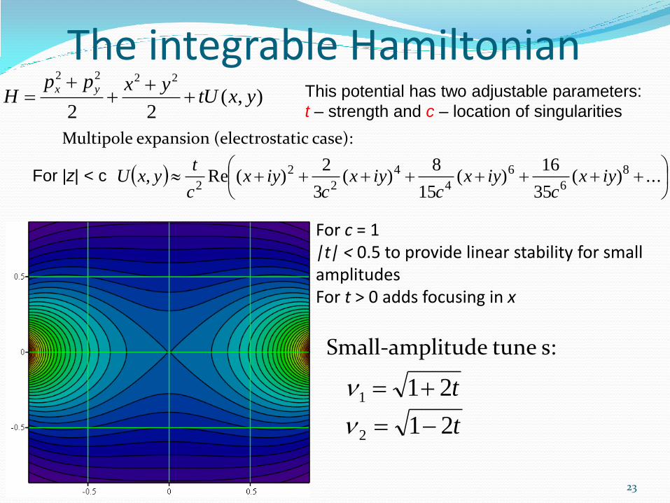
The integrable Hamiltonian
23
),(22
2222
yxtUyxpp
Hyx
Multipole expansion (electrostatic case):
For c = 1 |t| < 0.5 to provide linear stability for small amplitudes For t > 0 adds focusing in x
Small-amplitude tune s:
t
t
21
21
2
1
B
This potential has two adjustable parameters:
t – strength and c – location of singularities
...)(
35
16)(
15
8)(
3
2)(Re, 8
6
6
4
4
2
2
2iyx
ciyx
ciyx
ciyx
c
tyxUFor |z| < c

24
Magnetostatic case
B
...)(
35
16)(
15
8)(
3
2)(Im, 8
6
6
4
4
2
2
2iyx
ciyx
ciyx
ciyx
c
tyxUFor |z| < c

Convex Hamiltonian
This Hamiltonian is convex (steep)
Example of tunes for t = 0.4
25
0 0.2 0.4 0.6 0.8 10
1
2
w1j
1 2 t
J1 j
0 0.2 0.4 0.6 0.80
0.2
0.4
0.6
0.8
w2j
1 2 t
J2 j
ν1(J1, 0) ν2(0, J2)
t21 t21
For t -> 0.5 tune spreads of ~ 100% is possible

How to realize it?
Need to create an element
of periodicity.
The T-insert can also be
which results in a phase advance 0.5 (180 degrees) for the T-insert.
The drift space L can give the phase advance of at most 0.5 (180 degrees).
26
sL
β(s)T insert
100
0100
001
0001
k
k
100
0100
001
0001
k
k

How to make the Hamiltonian time-independent?
Example: quadrupoles
22
2,, yx
s
qsyxV
22),( NNNN yxqyxU
27 0 0.2 0.4 0.6 0.8
0
0.5
1
1.5
2
s( )
q s( )
s
β(s)
quadrupole amplitude
222222
22NN
NNyNxN
N yxqyxpp
H
L
Tunes:
)21(
)21(2
0
2
2
0
2
q
q
y
x
Tune spread: zero
Integrable but still linear…
)(,)(,)()(
22
2222
syxVyxpp
H NNNNyNxN
N

Possible location at Fermilab
28
Existing NML building Photoinjector and low energy test beamlines
up to 6 cryomodules High energy test
beamlines
New tunnel extension
New cryoplant and horizontal cryomodule
test stands
Possible 10m storage ring
75 meters

29
Nonlinear Lens Block
mx,my=0.5
x
y
Dx
e- Energy 150 MeV
Circumference 38 m
Dipole field 0.5 T
Betatron tunes Qx=Qy=3.2 (2.4 to 3.6)
Radiation damping time 1-2 s (107 turns)
Equilibrium emittance, rms, non-norm
0.06 mm
Nonlinear lens block
Length 2.5 m
Number of elements
20
Element length 0.1 m
Max. gradient 1 T/m
Pole-to-pole distance (min)
~ 2 cm

30
Non-linear elements section Number of elements per section: 20 – 30
Section length: 2 -3 m
30
Thu Oct 21 15:20:08 2010 OptiM - MAIN: - C:\Documents and S ettings\nsergei\My Documents\Papers\Invariants\IOTA\
50
50
BE
TA
_X
&Y
[m]
DIS
P_X
&Y
[m]
BE TA_X BE TA_Y DIS P_X DIS P_Y 0
0.05
0.1
0.15
0.2
0.25
0.3
1 2 3 4 5 6 7 8 9 10 11 12 13 14 15 16 17 18 19 20
Quadrupole component strength (T/m)

How to make these elements?
31
Proposal 1: custom-built magnet
Proposal 2: multipole expansion

Phase space with t<0.5, r<c
32
At Ax,Ay<0.5c trajectories remain inside r=c circle. Multipole expansion is valid.

Phase space with t<0.5, r>c
33
Motion is stable. Can not use multipole expansion of the potential.

Phase space with t>0.5
34
y=0 is unstable point. Still, it is possible to contain trajectories with x<c but y>c
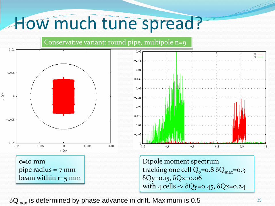
How much tune spread?
35
c=10 mm pipe radius = 7 mm beam within r=5 mm
Dipole moment spectrum tracking one cell Q0=0.8 dQmax=0.3 dQy=0.15, dQx=0.06 with 4 cells -> dQy=0.45, dQx=0.24
Conservative variant: round pipe, multipole n=9
dQmax is determined by phase advance in drift. Maximum is 0.5

How much tune spread?
36
c=10 mm pipe size x=5 y=35 mm beam within x=2 mm
Dipole moment spectrum tracking one cell Q0=0.8 dQmax=0.3 dQy=0.25, dQx=0.12 with 4 cells -> dQy=1, dQx=0.48
Less conservative variant: ‘true’ lens, t<0.5

How much tune spread?
37
c=10 mm pipe size x=5 y=35 mm beam within x=2.5 mm
Dipole moment spectrum tracking one cell Q0=0.8 dQmax=0.5 dQy=0.5, dQx=0.2 with 4 cells -> dQy=2, dQx=0.8
Full blast: ‘true’ lens, t=1.5

Effects of imperfections
38
c=10 mm pipe radius = 7 mm beam within r=5 mm dQy=0.4, dQx=0.2
Stability is preserved with •Transverse misalignments r.m.s. up to 0.5 mm •Synchrotron oscillations sE0.001, C=-15 •x/y difference up to 10% •mx≠my≠0.5 up to 0.01 •Sextupoles in the arcs DAx=c
Conservative variant: round pipe, multipole n=9

39
Current and Proposed Studies Numerical Simulations
Nonlinear lenses implemented in a multi-particle tracking code (MAD-X and PTC)
Studied particle stability Effects of imperfections (phase
advance, beta-functions, etc.) - acceptable
Synchrotron motion - acceptable Number of nonlinear lenses - 20
Simulated observable tune spread To Do:
Ring nonlinearities Chromaticity
Possible Experiments at Test Ring Demonstrate large betatron tune
spread
Demonstrate part of the beam crossing integer resonance
Map phase space with pencil beam by varying an injection error
Spectrum of horizontal dipole moment Q0=0.9x4=3.6 5000 particles 8000 revolutions But up to 106 revolutions simulated
All particles are stable!

40
Fermilab interests
Academic:
no resonances
long-term stability at large amplitudes
large tune spreads – Landau damping
Practical:
Electron machines
large dynamic apertures
Proton machines
super-high currents
instability damping
Relevant to DOE/HEP

Conclusions We found first examples of completely integrable non-
linear optics. Tune spreads of 50% are possible. In our test ring
simulation we achieved tune spread of about 1.5 (out of 3.6);
Nonlinear “integrable” accelerator optics has advanced to possible practical implementations Provides “infinite” Landau damping
Potential to make an order of magnitude jump in beam brightness and intensity
Fermilab is in a good position to use of all these developments for next accelerator projects
Rings or linacs
41

Acknowledgements Many thanks to:
Etienne Forest (KEK) for element implementation in PTC
Frank Schmidt (CERN) for optics implementation in MAD-X
Vladimir Kashiknin (FNAL) and Holger Witte (Oxford) for magnet proposals
42

Extra slides
43

Example of time-independent Hamiltonians Octupole
44
2
3
44,,
2244
3
yxyx
ssyxV
2
3
44
2244
NNNN xyyxU
This Hamiltonian is NOT integrable
Tune spread (in both x and y) is limited to ~12%
22442222 64
)(2
1)(
2
1yxyx
kyxppH yx
B

Example of integrable nonlinear Hamiltonian
This gives EXACT integrability
Not all trajectories encircle the singularity!
45
)(,)(,)()(
22
2222
syxVyxpp
H NNNNyNxN
N
222
22 2),(),(
yx
bxyyxayxUyxV
22
222 2
2yx
bxyyxaypxpI xy
2 1 0 1 24
2
0
2
4
pxi
xi
2 1 0 1 24
2
0
2
4
pyi
yi
2 1 0 1 22
1
0
1
2
yi
xi

46
Spectrum of vertical dipole moment. Q0=0.905x4=3.62