Rent sharing and the genderwage gap in Belgium

Francois Rycx and Ilan TojerowDepartment of Applied Economics (DULBEA), Free University of Brussels,

Brussels, Belgium

Keywords Pay differentials, Profits, Gender, Belgium

Abstract This study investigates, on the basis of a unique combination of two large-scale datasets, how rent sharing interacts with the gender wage gap in the Belgian private sector. Empiricalfindings show that individual gross hourly wages are significantly and positively related to firmprofits-per-employee even when controlling for group effects in the residuals, individual and firmcharacteristics, industry wage differentials and endogeneity of profits. Our instrumentedwage-profit elasticity is of the magnitude 0.06 and it is not significantly different for men andwomen. Of the overall gender wage gap (on average women earn 23.7 per cent less than men),results show that around 14 per cent can be explained by the fact that on average women areemployed in firms where profits-per-employee are lower. Thus, findings suggest that a substantialpart of the gender wage gap is attributable to the segregation of women in less profitable firms.

1. IntroductionSince Becker’s (1957) seminal paper on the economics of discrimination, studies on themagnitude and sources of the gender wage gap have proliferated (e.g. Blau and Kahn,2000). Numerous studies have, in particular, focused on the relationship betweenlabour market segregation and the gender wage differential (Carrington and Troske,1998; Fields and Wolff, 1995; Groshen, 1991; MacPherson and Hirsch, 1995; Rycx andTojerow, 2002). These papers examine basically to what extent the observed sex wagegap can be explained by occupational and sectoral segregation. Although the evidenceis still inconclusive, these studies show that a large fraction of the gender wage gap isaccounted for by segregation of women in lower-paying occupations, industries, andoccupations within establishments. Nevertheless, in contrast to previous research,Bayard et al. (1999) suggest that a substantial part of the sex wage gap remainsattributable to the individual’s sex.

Besides, there is a growing literature, essentially concentrated on the Anglo-Saxoncountries, showing that firms share rents with their employees (Abowd, 1989; Abowdand Lemieux, 1993; Blanchflower et al., 1996; Carruth and Oswald, 1989; Christofidesand Oswald, 1992; Denny and Machin, 1991; Hildreth and Oswald, 1997; Van Reenen,1996). In other words, recent findings suggest that ceteris paribus profitable firms payhigher wages to their employees. For Britain, Canada and the US, the estimatedelasticities between wages and profits-per-employee range between 0.04 and 0.2,

The Emerald Research Register for this journal is available at The current issue and full text archive of this journal is available at

www.emeraldinsight.com/researchregister www.emeraldinsight.com/0143-7720.htm

This paper is produced as part of a TSER programme on Pay Inequalities and EconomicPerformance financed by the European Commission (Contract nr. HPSE-CT-1999-00040). It hasevolved from earlier drafts presented in Brussels (79th AEA conference, PIEP meeting at theULB), Sevilla (15th EALE conference) and London (PIEP meeting at the LSE). The authors wouldlike to thank all seminar participants, and in particular Lena Nekby, for their suggestions andcomments. The authors are most grateful to Statistics Belgium for giving access to the BelgianStructure of Earnings Survey and Structure of Business Survey.

Rent sharingand the gender

wage gap

279

International Journal of ManpowerVol. 25 No. 3/4, 2004

pp. 279-299q Emerald Group Publishing Limited

0143-7720DOI 10.1108/01437720410541407

depending on the quality of instruments used to control for the endogeneity of profits.Notice that weak instrumenting biases downward the effect of profits on worker’swages. Results for continental Europe, although not very numerous, tend in the samedirection. For example, using Swedish matched worker-firm data for 1981 and 1991,Arai (2001) reports that the elasticity of wages with respect to profits-per-employeeis of the magnitude 0.01. The existence of rent sharing has also been examined inFrance and Norway by Margolis and Salvanes (2001) on the basis of linkedemployer-employee panel data. Considering a large number of statistical and economicexplanations, the authors find that the estimated coefficient on profits is not significantin France, while it is small but statistically different from zero in Norway. Nevertheless,let us notice that, using a large cross-section of French manufacturing workers,Fakhfakh and FitzRoy (2002) report a significant wage-profit elasticity between 0.01and 0.02.

In sum, there is strong evidence supporting that workers’ wages depend upon thefirms’ ability to pay. Yet, very little is known about:

. the relative magnitude of the pay-profit elasticity for male and female workers;and

. the contribution of rent sharing to the overall gender wage gap.

Recent findings (e.g. Arai and Heyman, 2001; Fakhfakh and FitzRoy, 2002) suggest,however, that the relationship between wages and profits is not neutral with respect togender. For example, using a large Swedish matched employer-employee data set for1991 and 1995, Nekby (2002) finds that the wage-profit elasticity is about 30-60 per centlower for women than for men. The author also shows that gender differences in rentsharing account for less than 2 per cent of the overall gender wage gap.

The objective of this paper is to examine the interaction between rent sharing andthe gender wage gap in the Belgian private sector. The current evidence regarding thelevel and sources of the gender wage gap in Belgium is still far incomplete. Jepsen (2001)shows, on the basis of the 1994 and 1995 Panel Study of Belgian Households (PSBH),that the sex wage gap between full-time workers stands at around 15 per cent and thatonly a very small part of it can be explained by gender differences in endowments.In contrast, using the 1995 Structure of Earnings Survey (SES), Plasman et al. (2001)suggest that the wage gap between (all) men and women working in the Belgian privatesector reaches almost 22 per cent and that half of it is attributable to gender differencesin working conditions, individual and firm characteristics. Moreover, while theexistence of rent sharing has been recently highlighted for Belgium by Goos andKonings (2001), its impact on the gender pay differential is still unknown.

The present paper aims to partially fill this gap by investigating, on the basis ofa unique combination of two large-scale, matched employer-employee data sets (i.e. theSES and the Structure of Business Survey, SBS), how rent sharing interacts with thegender wage gap in the Belgian private sector. To do so, we first investigate howindividual gross hourly wages are related to firm profits-per-employee whencontrolling for group effects in the residuals, individual and firm characteristics(e.g. education, prior experience, tenure, sex, occupation, region, autonomy at work,type of contract, firm size, level of wage bargaining), industry wage differentials(Nace 3-digit level) and endogeneity of profits. Secondly, we examine whether theseresults vary for men and women. Finally, we analyse, on the basis of the Oaxaca (1973)

IJM25,3/4

280

and Blinder (1973) decomposition technique, what proportion of the overall genderwage gap can be attributed to:

. gender differences in mean profit levels of employing firms;

. differences between wage-profit elasticities for men and women; and

. differences by gender in all other factors, i.e. intercepts, working conditions,individual and firm characteristics.

The remainder of this paper is organised as follows. Section 2 presents the theoreticalmodel. Sections 3 and 4 describe the data set and the empirical findings. Section 5concludes.

2. Theoretical frameworkTwo models have become standard in the literature for the analysis of the impactof profits-per-employee on wages in a bargaining framework. These are theright-to-manage and the efficient bargaining models, so-named, respectively, byNickell and Andrews (1983) and McDonald and Solow (1981). In the right-to-managemodel, firms unilaterally determine employment, while wages are the result ofa confrontation between the objectives of the firm and of the employees. In the efficientbargaining model, bargaining takes place with respect to both employment and wages.While both models yield identical wage equations, they differ fundamentally in that inthe former employment is endogenous with respect to wages whereas in the latter it isexogenous. Nevertheless, they both suggest that wages are related to the firm’s abilityto pay, i.e. to the firm’s profitability (Pencavel, 1991).

In this paper, we rely on the right-to-manage model[1]. Hence, suppose a bargainingsituation where a firm’s real profit function is given by:

P ¼ RðLÞ2 WL ð1Þ

with P the real profits, R(L) the real revenue, W the real wage and L the employmentlevel. Also consider a risk-neutral group of workers, not necessarily a union, whichattempts to maximize the expected utility of a representative member, defined as:

U ¼L

NW þ 1 2

L

N

� �A ð2Þ

where N is the number of members in the group ð0 , L # N Þ and A the outside optionðW . AÞ: The outside option is the expected value of real revenue perceived by anindividual in the event of redundancy. It depends positively on the unemploymentbenefit and on the expected real wage that a worker would obtain elsewhere, andnegatively on the unemployment rate.

The model is solved backwards: the profit-maximizing firm determines theemployment level, given the bargained wage in the first stage of the game. The resultingdeal is represented by the maximisation of the generalised Nash bargain. This approachboils down to maximising the weighted product of both parties’ net gain, i.e. thedifference between levels of utility in the event of an agreement and in the event of noagreement. For a company, without fixed costs, the level of utility reached whenbargaining fails equals zero. Indeed, since we assume that all workers are affiliated tothe group, the company will have to cease production if agreement is not reached.

Rent sharingand the gender

wage gap

281

The fallback position of a representative member of the group is equal to A. Accordingly,the generalised Nash bargaining problem can be written as follows (see Nickell, 1999, p. 3for a discussion on the notation)

WMaxUbP ¼

WMax

L

NðW 2 AÞ

� �bðRðLÞ2 WLÞ s:t: R0ðLÞ ¼ W ð3Þ

with b [ ½0; 1� the relative bargaining power of the workers in the wage bargain. Thefirst order condition of this problem is given by:

W ¼ A þ bðRðLÞ2 WLÞ

Lð4Þ

Expression (4) suggests that real wages are affected by the outside option, realprofits-per-employee and the relative bargaining power of the workers.

The corresponding statistical specification, which will serve as a benchmark for ourempirical analysis, can be written as follows:

Wi ¼ d0 þ d1URs þ d2SW s þ lP

L

� �f

þ1i ð5Þ

with Wi the logarithm of the gross hourly wage of the individual iði ¼ 1; . . . ;N Þ; URs thelogarithm of the unemployment rate in sector s; SWs the logarithm of the averageindividual gross hourly wage in sector s; (P/L)f the logarithm of the profits-per-worker infirm f; d0; d1, d2 and l are the parameters to be estimated and 1i is a white noise errorterm. URs and SWs reflect the outside option of a representative worker and (P/L)fcaptures the firm’s good fortune. According to bargaining theory, an increase in theoutside option of a representative worker reduces wage moderation. Therefore, weexpect a negative sign for d1 and a positive sign for d2. The intuition behind this is thatwhen the sector unemployment rate diminishes, the probability of finding a jobelsewhere goes up and therefore wage claims increase. In contrast, a drop in the expectedalternative wage mitigates envy effects and wage claims. l measures the relativebargaining power of the workers. The sign of the latter is expected to be positive andsome theories suggest that its magnitude may be different for men and women.

According to the theoretical model developed by Sap (1993), gender differences in lsmay appear if the bargaining position of the union is mainly reflective of the maleworkers’ interests. In other words, the biased composition of the union may generatea more favourable bargaining outcome for men. At the individual bargaining level,differences in rent sharing can also arise if men are more proficient than women atbargaining over wages (Nekby, 2002). Finally, differences in ls can be explained bythe fact that male workers are more present in capital-intensive firms. This explanation,based on Katz and Summers (1989) argument, implies that workers in highercapital-intensive industries have more power to extort rents during wage bargaining.

3. Description of the dataThe present study is based upon a unique combination of two large-scale data sets. Thefirst, carried out by Statistics Belgium, is the 1995 SES. It covers the Belgianestablishments employing at least ten workers and whose economic activities fall withinsections C to K of the Nace Rev.1 nomenclature[2]. The survey contains a wealth of

IJM25,3/4

282

information, provided by the management of the establishments, both on thecharacteristics of the latter (e.g. sector of activity, region, size of the establishment, levelof wage bargaining) and on the individuals working there (e.g. education, potentialexperience, seniority, gross hourly wages, bonuses, number of working hours paid,gender, occupation). Unfortunately, it provides no financial information. Therefore, theSES has been merged with the 1995 SBS. It is a firm-level survey, conducted by StatisticsBelgium, whose coverage differs from the SES in that it includes neither the financialsector (Nace J) nor the establishments with less than 20 employees. The SBS providesfirm-level information on financial variables such as sales, value added, value ofproduction, gross operating surplus and value of acquired goods and services. The finalsample, combining both data sets, covers 34,972 individuals working for 1,501 firms. It isrepresentative of all firms employing at least 20 workers within sections C to K of theNace Rev.1 nomenclature, with the exception of the financial sector.

Table I sets out the means (standard deviations) of selected variables for the overallsample as well as for men and women. We note a clear-cut difference betweenthe average characteristics of male and female workers. The point is that on average

Overall sample Men Women

Gross hourly wage (BEF)a 543.07 581.17 447.74(262.60) (281.79) (173.49)

Profits-per-worker (BEF)b 854.492 926.916 623.279(1,375.90) (1,342.81) (1,439.54)

Sector average gross hourly wage (in BEF)c 477.17 485.92 455.26(76.52) (71.44) (84.06)

Sector unemployment rate (in per cent)c,d 13.77 13.28 15.01(4.65) (4.33) (5.16)

Prior potential experience (years)e 9.20 9.37 8.77(8.18) (8.14) (8.26)

Seniority in the current company (years) 10.14 10.66 8.84(8.87) (9.09) (8.14)

Size of the establishmentf 645.49 767.74 339.58(1,331.53) (1,494.85) (697.85)

Hoursg 160.20 166.65 144.08(28.74) (21.10) (37.63)

Female (yes) 0.29 0.00 1.00Overtime paid (yes) 0.09 0.12 0.03Bonuses for shift work, night workand/or weekend work (yes) 0.21 0.26 0.10Number of observations in the sample 34,972 26,650 8,322

Notes: The descriptive statistics refer to the weighted sample. aIncludes overtime paid, premiums forshift work, night work and/or weekend work and bonuses (i.e. irregular payments which do not occurduring each pay period, such as pay for holiday, 13th month, profit sharing, etc.). 1 Euro ¼ 40.3399BEF; bApproximated by the firm annual gross operating surplus per worker. The gross operatingsurplus corresponds to the difference between the value added at factor costs and the total personnelexpenses. This variable is expressed in thousands of BEF; cSectors are defined at the Nace 2 digit level;dThe data relative to the sectoral unemployment rate were taken from the monthly bulletin of labourstatistics, published by the ONEM (1995); eExperience (potentially) accumulated on the labour marketbefore the last job. It has been computed as follows: age 2 6 2 years of education 2 seniority;fNumber of workers; gNumber of hours paid in the reference period, including overtime paid

Table I.Means (standard

deviations) of selectedvariables

Rent sharingand the gender

wage gap

283

men who earn significantly higher wages, are employed in larger firms whereprofits-per-capita are higher, work a larger number of (paid) hours, and have more(potential) experience and seniority. Also noteworthy is that while the average sectoralunemployment rate is smaller for men, the average sectoral wage is less important forwomen. Finally, Table I shows that the proportion of workers being paid a bonusfor overtime or shift work, night work and/or weekend work is significantly largeramong men (see Appendix 1 for a more detailed description).

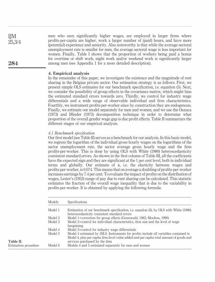
4. Empirical analysisIn the remainder of this paper, we investigate the existence and the magnitude of rentsharing in the Belgian private sector. Our estimation strategy is as follows. First, wepresent simple OLS estimates for our benchmark specification, i.e. equation (5). Next,we consider the possibility of group effects in the covariance matrix, which might biasthe estimated standard errors towards zero. Thirdly, we control for industry wagedifferentials and a wide range of observable individual and firm characteristics.Fourthly, we instrument profits-per-worker since by construction they are endogenous.Finally, we estimate our model separately for men and women, and we use the Oaxaca(1973) and Blinder (1973) decomposition technique in order to determine whatproportion of the overall gender wage gap is due profit effects. Table II summarizes thedifferent stages of our empirical analysis.

4.1 Benchmark specificationOur first model (see Table II) serves as a benchmark for our analysis. In this basic model,we regress the logarithm of the individual gross hourly wages on the logarithms of thesector unemployment rate, the sector average gross hourly wage and the firmprofits-per-worker. This is done by using OLS with White (1980) heteroscedasticityconsistent standard errors. As shown in the first column of Table III, all the coefficientshave the expected sign and they are significant at the 1 per cent level, both in individualterms and globally. Our estimate of l, i.e. the elasticity between wages andprofits-per-worker, is 0.074. This means that on average a doubling of profits-per-workerincreases earnings by 7.4 per cent. To evaluate the impact of profits on the distribution ofwages, Lester’s (1952) range of pay due to rent sharing can be calculated. This statisticestimates the fraction of the overall wage inequality that is due to the variability inprofits-per-worker. It is obtained by applying the following formula:

Models Specifications

Model 1 Estimation of our benchmark specification, i.e. equation (5), by OLS with White (1980)heteroscedasticity consistent standard errors

Model 2 Model 1+correction for group effects (Greenwald, 1983; Moulton, 1990)Model 3 Model 2+control for individual characteristics, firm size and the level of wage

bargainingModel 4 Model 3+control for industry wage differentialsModel 5 Model 4 estimated by 2SLS. Instruments for profits include all variables contained in

Model 4, plus per capita firm-level value added and per capita total amount of goods andservices purchased by the firm

Model 6 Models 4 and 5 estimated separately for men and womenTable II.Estimation procedure

IJM25,3/4

284

4lsðXÞ

Xð6Þ

where l is the estimated wage-profit elasticity, X measures the level of firmprofits-per-worker, and s (X) and X denote the standard deviation and the mean valueof X, respectively. On the basis of this formula, it appears that about 48 per cent of thevariance in individual wages is due to the variability in profits[3]. To put it another way,given that the mean hourly wage stands at BEF 543, rent sharing explains the variationof wages between BEF 284 and BEF 802[4].

Our benchmark regression clearly supports the hypothesis that individual wagesare significantly and positively related to the firm’s ability to pay. Nevertheless,caution is required. Indeed, the explanatory power of Model 1 is limited. The adjustedR 2 reaches only 0.21. Moreover, results might suffer from various econometric

OLS 2SLSVariables/models (1) (2) (3) (4) (5)

Intercept 1.946** 1.946** 4.367** 4.162** 5.085**(21.35) (5.25) (18.45) (25.80) (26.36)

Profits-per-worker (ln)a 0.074** 0.074** 0.036** 0.029** 0.063**(39.49) (8.96) (8.11) (8.15) (11.71)

Sector unemployment rate (ln) 20.035** 20.035 20.010 20.129** 20.148**(27.37) (21.93) (20.89) (25.93) (27.02)

Sector average wage (ln) 0.624** 0.624** 0.218** 0.305** 0.139**(43.11) (10.43) (5.70) (11.98) (4.28)

Group effectsb No Yes Yes Yes YesIndividual characteristics and

working conditionsc No No Yes Yes YesFirm characteristicsd No No Yes Yes YesIndustry effects (149 dummies) No No No Yes YesAdjusted R 2 0.208 0.208 0.694 0.719 0.712F-test 1,786** 133** 270** 1,491** 1,967**Test of over identification

restrictionse – – – – 3.497(0.174)

Lester’s range of wages(per cent) 47.7 47.7 23.2 18.7 40.6

Number of observations 34,972 34,972 34,972 34,972 34,972Number of groups – 1,501 1,501 1,501 1,501

Notes: The dependent variable is the (Naperian) logarithm of the individual gross hourly wages.t-statistics are between brackets. Standard errors have been corrected for heteroscedasticity by themethod of White (1980); **/*: coefficient significant at 1 and 5 per cent, respectively; aApproximatedby the firm annual gross operating surplus per worker; bGroup effects estimations use the correctionfor common variance components within groups proposed by Greenwald (1983) and Moulton (1990);cSex, six dummies for education, prior potential experience, its square and its cube, seniority within thecurrent company and its square, a dummy for individuals with no seniority, dummy variableindicating whether the individual supervises other workers, a variable showing whether the individualreceived a bonus for shift work, night work and/or weekend work, a dummy for overtime paid, threedummies for the type of contract, two regional dummies and 23 occupational dummies; dThe size of theestablishment and the level of wage bargaining (two dummies); eNR02 and associated ( p-value)

Table III.Earnings equations for all

workers

Rent sharingand the gender

wage gap

285

problems, e.g. group effects in the residuals, omitted variable biases, endogeneity ofprofits. In the next sections, we will therefore try to improve the robustness of ourmodel by controlling for these statistical issues.

4.2 Group effectsThe first potential trap derives from the simultaneous use of grouped observations andindividual data. Indeed, the presence of aggregate explanatory variables in Model 1 canbias the estimated standard errors and as a result distorts the significance of ourcoefficients. To account for these group effects, Model 2 applies the correction forcommon variance components within groups, as suggested by Greenwald (1983)and Moulton (1990). This correction transforms the covariance matrix of the errors,but leaves the point estimates and the determination coefficient unaffected. Therefore,our second model has the same estimated coefficients than our benchmark model, butdifferent t-statistics. Findings, reported in column (2) of Table III, clearly support theoverestimation phenomenon demonstrated by Moulton (1990). However, all regressioncoefficients, except that of unemployment, remain significant at the 1 per cent level.Therefore, it appears that the positive and significant relationship between wages andprofits cannot be attributed to group effects[5].

4.3 Individual and firm characteristicsThe omitted variable bias is another important issue that has to be investigated.According to the standard Walrasian (competitive) model of the labour market, wherethe equilibrium wage is determined through marginal productivity, two agents withidentical productive characteristics necessarily receive the same wages. However, theso-called compensating differences may occur between similar individuals placed indifferent working conditions. Indeed, the disutility undergone by one individualfollowing the performance of a task in an unfavourable situation may lead to wagecompensation. In accordance with this simple description of the wage determinationprocess, variables reflective of the productivity of the workers and their workingconditions have been added to our model. These include seven indicators showing thehighest level of education; prior potential experience, its square and its cube; senioritywithin the current company and its square; a dummy variable controlling for entrants,i.e. individuals with no seniority; the number of hours paid; a dummy for extra paidhours; 22 occupational dummies; three dummies for the type of contract; an indicatorshowing whether the individual is paid a bonus for shift work, night-time and/orweekend work and a dichotomic variable showing whether the individual supervisesother workers. Moreover, in order to control for gender and regional wage differentials,which are well documented in the literature (e.g. Farber and Newman, 1989; OECD,2002), we have also included a dummy for the sex of the individual and two regionaldummies indicating whether the establishment is located. Finally, in line with recentlabour market theories, supporting the existence of an effect of the employer’scharacteristics on wages, the size of the establishment and two dummies showing thelevel of wage bargaining have also been inserted in our regression.

The results relative to this new specification are presented in the third column ofTable III. We find that the wage-profit elasticity is still significant at the 1 per cent levelbut that its magnitude decreases from 0.074 to 0.036. As a result, Lester’s (1952) rangeof pay due to rent sharing drops from 48 to 23 per cent. Let us also notice that

IJM25,3/4

286

the inclusion of individual and firm characteristics has a substantial impact onthe explanatory power of the model. Indeed, the adjusted R 2 reaches now almost70 per cent.

In sum, results suggest that the positive and significant relationship between wagesand profits does not derive from an omitted variable bias. Yet, the absence of specificcontrol variables for the sectoral affiliation of the workers may be problematic.

4.4 Industry wage differentialsThe empirical debate about the causes of earnings inequalities was reopened at the endof the 1980s by an article by Krueger and Summers (1988). The authors showed thatwage disparities persisted in the US among workers with apparently identicalindividual characteristics and working conditions, employed in different sectors.Since then, similar results have been obtained for numerous industrialised countries(e.g. Goux and Maurin, 1999; Hartog et al., 1997; Rycx, 2002; Vainiomaki andLaaksonen, 1995). In light of this literature, it could be argued that rent sharing issimply reflective of industry wage premiums. In other words, it is possible that thepositive correlation between wages and profits is generated by sectoral shocks ratherthan by the division of firms’ rents. For this reason, 149 dummy variables indicatingthe sectoral affiliation of the workers have been added to our model. The results of thisnew specification are presented in column 4 of Table III. As expected, we find thatsectors have a significant impact on the wage-profit elasticity. Indeed, the coefficient onprofits drops from 0.036 in Model 3 to 0.029 in the current frame. However, rent sharingis still significant at the 1 per cent level and the adjusted R 2 reaches now more than70 per cent. Moreover, from Appendix 2, it can be seen that all other coefficients havethe expected sign and that the vast majority of them are significant at the 5 per centlevel.

4.5 Endogeneity of profitsAlthough Model 4 seems quite accurate, it still suffers from a serious problem, namelythe endogeneity of profits. Indeed, by construction, wages have a negative impacton profits. Therefore, earlier OLS estimates are not only biased but also inconsistent.To bypass this problem, we estimated Model 4 using the method of instrumentalvariables. This method consists in findings instruments, which are at the same timehighly correlated with the endogenous variable and uncorrelated with the error term.We used as instruments for profits all the variables contained in Model 4, plus percapita firm level value added and per capita total amount of goods and servicespurchased by the firm. Results of our 2SLS regression are presented in the last columnof Table III[6]. Not surprisingly, we find that the wage-profit elasticity increases from0.029 to 0.063, which confirms the downward biasness of our previous estimates[7].It follows that Lester’s range of pay is about 42 per cent of the mean wage.

Yet, it could be argued that the instruments that have been used are inappropriate.To check for this, Sargan’s (1964) over-identification test has been used. Thecorresponding test statistic is computed as NR02, where N is the number ofobservations and R02 is the per cent of variation explained in the regression of theresiduals from the second-stage equation on the instruments and all exogenousvariables in the model. This statistic is distributed x2 with degrees of freedom equal tothe number of overidentifying restrictions (in this case, df ¼ 2). The results of this test,

Rent sharingand the gender

wage gap

287

presented at the bottom of column 5 in Table III, show that the overidentifyingrestrictions cannot be rejected at the level of 15 per cent. This suggests that ourinstruments are valid and that Model 5 is well specified.

Our findings are significantly smaller than those reported for Belgium by Goosand Konings (2001). Indeed, the latter report a wage-profit elasticity of around 0.10and a Lester’s range of pay of approximately 60 per cent of the mean wage.Nevertheless, many factors can explain these differences. First, Goos and Koningsonly include a very limited number of control variables in their analysis, namely theratio of white- over blue-collar workers and one digit industry dummies. Secondly,they use pooled data regressions covering the period 1987-1994, while the presentstudy relies on a single cross-section relative to 1995. Thirdly, their data set has alarger coverage than ours. In particular, it covers the financial sector, where rentsharing is expected to be relatively high. Fourthly, they instrument profits by theirlagged values when we rely on a whole set of instrumental variables including percapita firm level value added and per capita total amount of goods and servicespurchased by the firm. Finally, let us also notice that their dependent variable is lessprecise since it is constructed by dividing annual labour costs by the number ofemployees in the firm. Be that as it may, both studies suggest that rent sharing existsin Belgium and that a substantial part of the dispersion in wages is due to thevariability in profits.

4.6 Rent sharing for men and womenSo far, the existence and magnitude of rent-sharing in the Belgian private sector hasbeen investigated for all workers, independently of their sex. In this section, we analyseif the wage-profit elasticity is significantly different for male and female workers andwe decompose the overall gender wage gap to determine what proportion is due rentsharing.

4.6.1 Wage-profit elasticities by gender. To investigate the interaction between rentsharing and gender, Models 4 and 5 have been estimated separately for men andwomen[8]. The results from this analysis are reported in Table IV and Appendix 3.As mentioned earlier, the OLS estimates are inconsistent because of the endogeneity ofprofits. Therefore, we focus on the 2SLS results[9].

For both sexes, we find that the coefficients on profits-per-worker are significantat the 1 per cent level. In addition, profit effects look approximately 10 per cent higherfor men than for women. Indeed, the wage-profit elasticity stands at 0.059 for womenand at 0.066 for men. Yet, using a standard t-test, we find no significant differencebetween the regression coefficients of both sexes[10]. Hence, there appears to beno gender difference in remuneration from firm profits. Finally, let us notice thatLester’s (1952) range of pay due to rent sharing equals, respectively, 38.2 and 56.2 per centfor men and women.

4.6.2 Decomposition of the gender wage gap. To complete our analysis, wedecomposed the overall gender wage gap in order to assess what proportion is due to:

(1) differences between female and male wage-profit elasticities;

(2) differences by gender in the average value of firm profits-per-capita; and

(3) differences by gender in all other factors, i.e. intercepts, inter-industry wagedifferentials, working conditions, individual and firm characteristics.

IJM25,3/4

288

To do so, we used the decomposition procedure developed by Oaxaca (1973) andBlinder (1973), who showed that the difference between the average hourly wage(in logarithms) of men and women can be broken as follows:

Wm 2 Wf ¼P

L

� �f

lm 2 lf

� �þ

P

L

� �m

2P

L

� �f

!lm þ X f qm 2 qf

� �

þ Xm 2 X f

� �qm ð7Þ

or

Wm 2 Wf ¼P

L

� �m

lm 2 lf

� �þ

P

L

� �m

2P

L

� �f

!lf þ Xm qm 2 qf

� �

þ Xm 2 X f

� �qf ð8Þ

where the indices m and f refer, respectively, to male and female workers, W representsthe average (Naperian logarithm) of the hourly wage, ðP=LÞ is the average value of

Model 4 (OLS) Model 5 (2SLS)Variables/models Men Women Men Women

Intercept 5.738** 5.424** 5.631** 5.270**(45.45) (73.15) (45.35) (61.93)

Profits-per-worker (ln)a 0.030** 0.025** 0.066** 0.059**(8.30) (4.71) (12.81) (6.68)

Sector unemployment rate (ln) No No No NoSector average wage (ln) No No No NoGroup effectsb Yes Yes Yes YesIndividual characteristics and working conditionsc Yes Yes Yes YesFirm characteristicsd Yes Yes Yes YesIndustry effects (149 dummies) Yes Yes Yes YesAdjusted R 2 0.709 0.678 0.702 0.669F-test 1,348** 1,544** 624** 1,506**Test of over identification restrictionse – – 5.330 1.664

(0.069) (0.435)Lester (1952) range of wages (per cent) 17.4 21.4 38.2 50.4Number of observations 26,650 8,322 26,650 8,322Number of groups 1,475 1,217 1,475 1,217

Notes: The dependent variable is the (Naperian) logarithm of the individual gross hourly wages.t-statistics are between brackets. Standard errors have been corrected for heteroscedasticity by themethod of White (1980). **/*: coefficient significant at 1 and 5 per cent, respectively; aApproximatedby the firm annual gross operating surplus per worker; bGroup effects estimations use the correctionfor common variance components within groups proposed by Greenwald (1983) and Moulton (1990);cSex; six dummies for education; prior potential experience, its square and its cube; seniority within thecurrent company and its square, a dummy for individuals with no seniority; dummy variableindicating whether the individual supervises other workers; a variable showing whether the individualreceived a bonus for shift work, night work and/or weekend work, a dummy for overtime paid, threedummies for the type of contract, two regional dummies and 23 occupational dummies; dThe size of theestablishment and the level of wage bargaining (two dummies); eNR02 and associated ( p-value)

Table IV.Men and women, OLSversus 2SLS estimates

Rent sharingand the gender

wage gap

289

firm profits-per-capita and X is a vector containing an intercept and the average valuesof the individual characteristics of the workers, their working conditions, their sectoralaffiliation, the size of their establishment and the level of wage bargaining therein.q and l are the 2SLS regression coefficients relative to ðP=LÞ and X reported inTable IV and Appendix III. Equations (6) and (7) take as a non-discriminatory wagestructure that of men and women, respectively.

As shown in Table V, the overall gender wage gap, measured as the differencebetween mean log wages of male and female workers, stands at 0.237. This means thatthe average female worker earns 76.3 per cent of the mean male wage. Moreover,depending on the non-discriminatory wage structure used, results indicate thatbetween 12.7 and 14.3 per cent of the overall gender wage gap can be explained by thefact that on average women are employed in firms where profits-per-employee arelower. Table V also suggests that around 18 per cent of the overall gender wage gapderives from differences between wage-profit elasticities for men and women.However, the latter result should be interpreted with caution because the wage-profitelasticity is not significantly different for both sexes.

5. ConclusionThis paper investigates, on the basis of a unique combination of two large-scale datasets, how rent sharing interacts with the gender wage gap in the Belgian private sector.Empirical findings show that individual gross hourly wages are significantly andpositively related to firm profits-per-employee even when controlling for group effectsin the residuals, individual and firm characteristics, industry wage differentials andendogeneity of profits. Our instrumented wage-profit elasticity is of the magnitude0.06 and it is not significantly different for men and women. Of the overall gender wagegap (on average women earn 23.7 per cent less than men), results show that around14 per cent can be explained by the fact that on average women are employed in firmswhere profits-per-employee are lower. To put it differently, findings suggest thata substantial part of the gender wage gap is attributable to the segregation ofwomen in less profitable firms. Future research concerning the magnitude of rentsharing in Belgium should rely on matched employer-employee panel data so as tocontrol for the non-observed individual characteristics of the workers. Indeed, thesecharacteristics might modify our results if it emerged that they were not randomlydistributed between firms and or sexes. Unfortunately, at present such data set doesnot exist.

Percentage of overall wage gap due to differences in

Non-discriminatorywage structure

Overall genderwage gap:�Wm 2 �Wf

Average values of firmprofits per capita:

ððP=LÞm 2 ðP=LÞfÞlmðfÞ

Wage-profitselasticities:

ðP=LÞfðmÞðlm 2 lfÞ

Allother

factors

Male wagestructure 0.237 14.3 17.3 68.4Female wagestructure 0.237 12.7 18.9 68.4

Note: Computation based on the 2SLS estimates reported in Table IV

Table V.Decomposition of thegender wage gap

IJM25,3/4

290

Notes

1. Using Belgian aggregate data from 1957 to 1988, Vannetelbosch (1996) has shown that boththe right-to-manage and the efficient bargaining models can be rejected in favour of thegeneral bargaining model, developed by Manning (1987). This means that the outcome ofthe bargaining process is located somewhere between the labour demand curve and thecontract curve. Nevertheless, this result must be considered with caution for at least tworeasons. First, the estimates are very sensitive to the specification of the reservation wage,and second, the trade union density and the number of strikes are far from ideal as asurrogate for the relative bargaining power of unions. This uncertainty is not verysurprising since “the empirical literature has not yet been able to find an appropriate test todistinguish between the principal models” (Booth, 1995, p. 141). Also noteworthy is that,while these models have different implications for unemployment and economic welfare,they generate identical wage equations. Hence, for the sake of simplicity, we have chosen torely on the right-to-manage model.

2. The following sectors are therefore not part of the sample: agriculture, hunting and forestry;fisheries; public administration; education; health and social action; collective, social andpersonal services; domestic services; and extra-territorial bodies.

3. Notice that ½0:074 £ 4 £ ð1; 375:9=854:492Þ� £ 100 is equal to 47.7 per cent.

4. 1 Euro equals 40.3399 BEF.

5. Because of its substantial impact on the standard errors of the estimates, the correction forgroup effects has been applied to all other models presented in this paper.

6. Detailed results are shown in Appendix 2.

7. All coefficients in the first-stage regression are jointly significant at the 1 per cent level.Results are available on request.

8. Because of a strong multicollinearity problem, the sector average gross hourly wage andthe sector unemployment rate have been not been included in the regression.

9. Let us notice that the p-value relative to the over-identification test for the male regressionequals only 0.069.

10. For the 2SLS regressions (model 5), t ¼ 0:69:

References

Abowd, J.A. (1989), “The effect of wage bargaining on the stock market value of the firm”,American Economic Review, Vol. 79 No. 4, pp. 774-800.

Abowd, J.A. and Lemieux, T. (1993), “The effects of product market competition on collectivebargaining agreements: the case of foreign competition in Canada”, Quarterly Journal ofEconomics, Vol. 108 No. 4, pp. 983-1014.

Arai, M. (2001), “Wages, profits and capital intensity: evidence from matched worker-firm data”,Journal of Labour Economics, Vol. 21 No. 3, pp. 593-618.

Arai, M. and Heyman, F. (2001), “Wages, profits and individual unemployment risk: evidencefrom matched worker-firm data”, FIEF Working Paper Series, No. 172.

Bayard, J.M., Hellerstein, J., Neumark, D. and Troske, K. (1999), “New evidence on sexsegregation and sex difference in wages from matches employer-employee data”, NBERWorking Paper, No. 7003.

Becker, G. (1957), The Economics of Discrimination, University of Chicago Press, Chicago, IL.

Blanchflower, D.G., Oswald, A.J. and Sanfey, P. (1996), “Wages, profits and rent-sharing”,Quarterly Journal of Economics, Vol. 111 No. 1, pp. 227-51.

Rent sharingand the gender

wage gap

291

Blau, F. and Kahn, L. (2000), “Gender differences in pay”, Journal of Economic Perspectives,Vol. 14 No. 4, pp. 75-99.

Blinder, A. (1973), “Wage discrimination: reduced form and structural variables”, Journal ofHuman Resources, Vol. 8 No. 4, pp. 436-65.

Booth, A. (1995), The Economics of the Trade Union, Cambridge University Press, Cambridge.

Carrington, W. and Troske, K. (1998), “Sex segregation in US manufacturing”, Industrial andLabor Relations Review, Vol. 51 No. 3, pp. 445-64.

Carruth, A.A. and Oswald, A.J. (1989), Pay Determination and Industrial Prosperity, ClarendonPress, Oxford.

Christofides, L.N. and Oswald, A.J. (1992), “Real wage determination and rent-sharing incollective bargaining agreements”, Quarterly Journal of Economics, Vol. 107 No. 3,pp. 985-1002.

Denny, K. and Machin, S. (1991), “The role of profitability and industrial wages in firm-levelwage determination”, Fiscal Studies, Vol. 12, pp. 34-45.

Fakhfakh, F. and FitzRoy, F. (2002), “Basic wages and firm characteristics: rent-sharing inFrench manufacturing”, mimeo, ERMES, Universite de Paris II.

Farber, S. and Newman, R. (1989), “Regional wage differentials and the special convergenceof worker characteristics prices”, Review of Economics and Statistics, Vol. 71 No. 2,pp. 224-31.

Fields, J. and Wolff, E. (1995), “Interindustry wage differentials and the gender wage gap”,Industrial and Labor Relations Review, Vol. 49 No. 1, pp. 105-20.

Goos, M. and Konings, J. (2001), “Does rent-sharing exist in Belgium? An empirical analysisusing firm level data”, Reflets et perspectives de la vie economiques, Vol. XL No. 1-2,pp. 65-79.

Goux, D. and Maurin, E. (1999), “Persistence of interindustry wage differentials: a reexaminationusing matched worker-firm panel data”, Journal of Labor Economics, Vol. 17 No. 3,pp. 492-533.

Greenwald, B.C. (1983), “A general analysis of bias in the estimated standard errors of leastsquare coefficients”, Journal of Econometrics, Vol. 22 No. 3, pp. 323-38.

Groshen, E.L. (1991), “The structure of the female/male wage differential: is it who youare, what you do, or where you work?”, Journal of Human Resources, Vol. 26 No. 3,pp. 457-72.

Hartog, J., Van Opstal, R. and Teulings, C. (1997), “Inter-industry wage differentials and tenureeffects in The Netherlands and the US”, De Economist, Vol. 145 No. 1, pp. 91-9.

Hildreth, A.K.G. and Oswald, A.J. (1997), “Rent-sharing and wages: evidence from company andestablishment panels”, Journal of Labor Economics, Vol. 15 No. 2, pp. 318-37.

Jepsen, M. (2001), “Evaluation des differentiels salariaux en Belgique: homme-femme ettemps partiel-temps plein”, Reflets et Perspectives de la vie economique, Vol. 40 No. 1-2,pp. 51-63.

Katz, L.F. and Summers, L.H. (1989), “Industry rents: evidence and implications”, BrookingPapers on Economic Activity, pp. 209-75, Special issue.

Krueger, A. and Summers, L. (1988), “Efficiency wages and inter-industry wage structure”,Econometrica, Vol. 56 No. 2, pp. 259-93.

Lester, R.A. (1952), “A range theory of wage differentials”, Industrial and Labour RelationsReview, Vol. 5 No. 4, pp. 483-500.

IJM25,3/4

292

MacPherson, D. and Hirsch, B. (1995), “Wages and gender composition: why do women’s jobspay less?”, Journal of Labor Economics, Vol. 13 No. 3, pp. 426-71.

Manning, A. (1987), “An integration of trade union models in a sequential bargainingframework”, Economic Journal, Vol. 97 No. 385, pp. 121-39.

Margolis, D.N. and Salvanes, K.G. (2001), “Do firms really share rents with their workers?”,CREST Working Paper, No. 2001-16.

Moulton, B.R. (1990), “An illustration of a pitfall in estimating the effects of aggregate variableson micro units”, Review of Economics and Statistics, Vol. 72 No. 2, pp. 334-8.

McDonald, I. and Solow, R. (1981), “Wage bargaining and employment”, American EconomicReview, Vol. 74 No. 5, pp. 896-908.

Nekby, L. (2002), “A note on gender differences in rent sharing and its implications for the genderwage gap”, mimeo, Trade Union Institute for Economic Research (FIEF) and Departmentof Economics, Stockholm University.

Nickell, S. (1999), “Product markets and labour markets”, Labour Economics, Vol. 6 No. 1,pp. 1-20.

Nickell, S. and Andrews, M. (1983), “Unions, real wages and employment in Britain 1951-79”,Oxford Economic Papers, Vol. 35 No. supplement, pp. 183-206.

Pencavel, J. (1991), Labor Markets under Trade Unionism. Employment, Wages and Hours,Blackwell publishers, Cambridge, MA.

Plasman, A., Plasman, R., Rusinek, M. and Rycx, F. (2001), “Indicators on gender pay equality”,Cahiers Economiques de Bruxelles, Vol. 45 No. 2, pp. 11-40.

Oaxaca, R. (1973), “Male-female wage differentials in urban labour markets”, InternationalEconomic Review, Vol. 14 No. 3, pp. 693-709.

OECD (2002), Employment Outlook, OECD, Paris.

ONEM (1995), Monthly Bulletion, Octobre issue, Brussels.

Rycx, F. (2002), “Inter-industry wage differentials: evidence from Belgium in a cross-nationalperspective”, De Economist, Vol. 150 No. 5, pp. 555-68.

Rycx, F. and Tojerow, I. (2002), “Inter-industry wage differentials and the gender wage gap inBelgium”, Cahiers Economiques de Bruxelles, Vol. 45 No. 2, pp. 119-41.

Sap, J. (1993), “Bargaining power and wages. A game-theoretic model of gender differences inunion wage bargaining”, Labour Economics, Vol. 1 No. 1, pp. 25-48.

Sargan, J.D. (1964), “Wages and prices in the United Kingdom: a study in econometricmethodology”, in Hart, P.E., Mills, G. and Whitaker, J.K. (Eds), Econometric Analysis forNational Economic Planning, Butterworths, London.

Vainiomaki, J. and Laaksonen, S. (1995), “Inter-industry wage differentials in Finland:evidence from longitudinal census data for 1975-85”, Labour Economics, Vol. 2 No. 2,pp. 161-73.

Vannetelbosch, V. (1996), “Testing between alternative wage-employment bargaining modelsusing Belgian aggregate data”, Labour Economics, Vol. 3 No. 1, pp. 43-64.

Van Reenen, J. (1996), “The creation and capture of rents: wages and innovation in a panel of UKcompanies”, Quarterly Journal of Economics, Vol. 111 No. 1, pp. 195-226.

White, H. (1980), “A heteroscedasticity-consistent covariance matrix estimator and a direct testfor heteroscedasticity”, Econometrica, Vol. 48 No. 4, pp. 817-30.

Rent sharingand the gender

wage gap

293

Appendix 1

Overallsample Men Women

Gross hourly wage: (in BEF) includes overtime paid, premiumsfor shift work, night work and/or weekend work and bonuses(i.e. irregular payments which do not occur during each pay period,such as pay for holiday, 13th month, profit sharing, etc.).1 Euro ¼ 40.3399 BEF 543.07 581.17 447.74

(262.60) (281.79) (173.49)

Profits-per-worker: (in BEF) approximated by the firm annual grossoperating surplus per worker. The gross operating surpluscorresponds to the difference between the value added at factorcosts and the total personnel expenses. This variable is expressedin thousands of BEF 854.492 926.916 623.279

(1,375.90) (1,342.81) (1,439.54)

Sector average gross hourly wage: (in BEF), sectors are defined atthe Nace 2 digit level 477.17 485.92 455.26

(76.52) (71.44) (84.06)Sector unemployment ratea: (in per cent), sectors are defined at theNace 2 digit level 13.77 13.28 15.01

(4.65) (4.33) (5.16)

Education:Primary or no degree: 0-6 years 11.4 11.6 11.0Lower secondary: 9 years 25.7 25.3 26.7General upper secondary: 12 years 16.2 13.0 24.1Technical/artistic/prof. upper secondary: 12 years 25.9 29.5 17.0Higher non-university short type, higher artistictraining: 14 years 12.4 11.3 15.3University and non-university higher education,long type: 16 years 7.9 8.9 5.5Post-graduate: 17 years or more 0.5 0.5 0.4

Prior potential experience: (years), experience (potentially)accumulated on the labour market before the last job. It has beencomputed as follows: age26 2 years of education 2 seniority 9.20 9.37 8.77

(8.18) (8.14) (8.26)Seniority in the current company: (years) 10.14 10.66 8.84

(8.87) (9.09) (8.14)

Size of the establishment: number of workers 645.49 767.74 339.58(1,331.53) (1,494.85) (697.85)

Hours: number of hours paid in the reference period, includingovertime paid 160.20 166.65 144.08

(28.74) (21.10) (37.63)Female (yes) 28.6 0.0 100Overtime paid (yes) 9.3 11.7 3.4Bonuses for shift work, night work and/or weekend work (yes) 21.0 25.5 9.7Supervises the work of other workers (yes) 15.6 18.2 8.9Type of contract:

Unlimited-term employment contract 96.8 97.4 95.4Limited-term employment contract 2.8 2.2 4.1

(continued )

Table AI.Description and means(standard deviations) ofselected variables

IJM25,3/4

294

Overallsample Men Women

Apprentice/trainee contract 0.1 0.1 0.2Other 0.3 0.3 0.4Region: geographic location of the establishment

Brussels 12.7 11.6 15.6Wallonia 20.4 19.5 22.7Flanders 66.9 69.0 61.7

Level of wage bargaining:Collective wage agreement only at the national and/or sectoral

level 47.1 44.4 53.8Collective wage agreement at the company level 46.3 49.3 38.7Other 6.6 6.3 7.5

Number of observations in the sample 34,972 26,650 8,322

Notes: The descriptive statistics refer to the weighted sample. Descriptive statistics relative to thesectoral affiliation of the workers and their occupations are available on request. aThe data relative tothe sectoral unemployment rate were taken from the monthly bulletin of labour statistics, published bythe ONEM (1995) Table AI.

Appendix 2

Variables/models Model 4 (OLS) Model 5 (2SLS)

Intercept 5.655** 4.162** 5.528** 5.085**(76.71) (25.80) (73.40) (73.40)

Profits-per-worker (ln)a 0.029** 0.029** 0.063** 0.063**(8.15) (8.15) (11.71) (11.71)

Sector unemployment rate (ln) – 20.129** – 20.148**(25.93) (27.02)

Sector average wage (ln) – 0.305** – 20.139**(11.98) (4.28)

EducationPrimary or no degree Reference Reference Reference ReferenceLower secondary 0.045** 0.045** 0.046** 0.046**

(4.71) (4.71) (4.76) (4.76)General upper secondary 0.143** 0.143** 0.144** 0.144**

(12.19) (12.19) (12.07) (12.07)Technical/artistic/prof. uppersecondary 0.143** 0.143** 0.142** 0.142**

(13.43) (13.43) (13.28) (13.28)Higher non university short type,higher artistic training 0.256** 0.256** 0.252** 0.252**

(18.79) (18.79) (18.42) (18.42)University and non-university highereducation, long type 0.417** 0.417** 0.414** 0.414**

(22.99) (22.99) (22.88) (22.88)Post-graduate 0.586** 0.586** 0.583** 0.583**

(12.20) (12.20) (12.34) (12.34)

(continued )

Table AII.Earnings equations for allworkers, detailed results

Rent sharingand the gender

wage gap

295

Variables/models Model 4 (OLS) Model 5 (2SLS)

Prior experienceSimple 0.016** 0.016** 0.016** 0.016**

(12.74) (12.74) (12.38) (12.38)Squared/102 20.039** 20.039** 20.037** 20.037**

(24.65) (24.65) (24.36) (24.36)Cubed/104 0.002 0.002 0.002 0.002

(1.455) (1.455) (1.23) (1.23)Individual with no seniority (yes) 20.036 20.036 20.045 20.045

(21.09) (21.09) (21.28) (21.28)Seniority in the company

Simple 0.019** 0.019** 0.019** 0.019**(22.47) (22.47) (21.62) (21.62)

Squared/102 20.024** 20.024** 20.024** 20.024**(29.72) (29.72) (29.30) (29.30)

Hours paid (ln) 20.043** 20.043** 20.056** 20.056**(23.35) (23.35) (24.48) (24.48)

Bonus for shift work, night work and/orweekend work (yes) 0.059** 0.059** 0.059** 0.059**

(7.21) (7.21) (7.08) (7.08)Overtime paid (yes) 0.021** 0.021** 0.016* 0.016*

(2.78) (2.78) (1.98) (1.98)Contract

Unlimited-term employmentcontract Reference Reference Reference ReferenceLimited-term employment contract 20.052** 20.052** 20.057** 20.057**

(23.77) (23.77) (24.11) (24.11)Apprentice/trainee contract 20.588** 20.588** 20.599** 20.599**

(23.29) (23.29) (23.38) (23.38)Other employment contract 20.082** 20.082** 20.071** 20.071**

(23.28) (23.28) (22.87) (22.87)Female (yes) 20.121** 20.121** 20.120** 20.120**

(217.87) (217.87) (217.62) (217.62)Occupation (23 dummies) Yes Yes Yes YesRegion

Brussels Reference Reference Reference ReferenceWallonia 20.016 20.016 20.009 20.009

(21.25) (21.25) (20.69) (20.69)Flanders 20.042** 20.042** 20.036** 20.036**

(23.72) (23.72) (23.03) (23.03)Supervises the work of co-workers (yes) 0.126** 0.126** 0.129** 0.129**

(13.76) (13.76) (13.74) (13.74)Size of the establishment (ln) 0.038** 0.038** 0.037** 0.037**

(9.45) (9.45) (9.09) (9.09)Level of wage bargaining

CA only at the national and/or sectorallevel Reference Reference Reference ReferenceCA at the company level 0.032** 0.032** 0.029** 0.029**

(2.97) (2.97) (2.76) (2.76)Other 20.009 20.009 20.014 20.014

(20.66) (20.66) (21.04) (21.04)

(continued )Table AII.

IJM25,3/4

296

Variables/models Model 4 (OLS) Model 5 (2SLS)

Industry effects (149 dummies) Yes Yes Yes YesGroup effects Yes Yes Yes YesTest of over-identification restrictionsb – – 3.497 3.497

(0.174) (0.174)R 2 adjusted 0.719 0.719 0.712 0.712F-test 3,728** 1,491** 590** 1,967**Number of observations 34,972 34,972 34,972 34,972Number of groups 1,501 1,501 1,501 1,501

Notes: The dependent variable is the (Naperian) logarithm of the individual gross hourly wages.t-statistics are between brackets. White (1980) heteroscedasticity consistent standard errors. Groupeffects estimations use the correction for common variance components within groups proposed byGreenwald (1983) and Moulton (1990). aApproximated by the firm annual gross operating surplus perworker. bNR

02 and associated ( p-value). **/*/***: coefficient significant at 1, 5 and 10 per cent,respectively Table AII.

Appendix 3

Model 4 (OLS) Model 5 (2SLS)Variables/models Men Women Men Women

Intercept 5.738** 4.697** 5.424** 5.563** 5.631** 5.270**(45.45) (10.44) (73.15) (7.79) (45.35) (61.93)

Profits-per-worker (ln)a 0.030** 0.030** 0.025** 0.025** 0.066** 0.059**(8.30) (8.30) (4.71) (4.71) (12.81) (6.68)

Sector unemploymentrate (ln) – 20.128** – 20.155** – –

(24.03) (23.57)Sector average wage (ln) – 0.229** – 0.447 – –

(3.07) (0.35)Education

Primary or no degree Reference Reference ReferenceLower secondary 0.057** 0.057** 0.020 0.020 0.056** 0.021

(5.30) (5.30) (1.70) (1.70) (5.20) (1.77)General upper secondary 0.142** 0.142** 0.135** 0.135** 0.142** 0.133**

(10.33) (10.33) (8.92) (8.92) (10.22) (8.72)Technical/artistic/prof.upper secondary 0.147** 0.147** 0.122** 0.122** 0.146** 0.121**

(11.84) (11.84) (7.76) (7.76) (11.70) (7.58)Higher non-universityshort type, higherartistic training 0.249** 0.249** 0.258** 0.258** 0.246** 0.250**

(16.58) (16.58) (13.69) (13.69) (16.11) (13.63)University andnon-university highereducation, long type 0.418** 0.418** 0.396** 0.396** 0.416** 0.388**

(22.18) (22.18) (14.19) (14.19) (21.78) (14.26)

(continued )

Table AIII.Earnings equations bygender, detailed results

Rent sharingand the gender

wage gap

297

Model 4 (OLS) Model 5 (2SLS)Variables/models Men Women Men Women

Post-graduate 0.587** 0.587** 0.554** 0.554** 0.584** 0.550**(10.41) (10.41) (8.49) (8.49) (10.53) (8.37)

Prior experienceSimple 0.015** 0.015** 0.020** 0.020** 0.014** 0.020*

(9.70) (9.70) (9.69) (9.69) (9.29) (9.55)Squared/102 20.024* 20.024* 20.072** 20.072** 20.021* 20.074**

(22.50) (22.50) (25.40) (25.40) (22.14) (25.43)Cubed/104 20.004 20.004 0.084** 0.084** 20.001 0.010**

(20.197) (20.197) (3.42) (3.42) (20.50) (3.46)Individual with no

seniority (yes) 20.024 20.024 20.064 20.064 20.037 20.069(20.73) (20.73) (21.26) (21.26) (21.11) (21.29)

Seniority in thecompanySimple 0.018** 0.018** 0.020** 0.020** 0.018** 0.020**

(20.16) (20.16) (12.28) (12.28) (19.79) (11.85)Squared/102 20.023** 20.023** 20.023** 20.023** 20.022** 20.024**

(28.82) (28.82) (24.33) (24.33) (28.52) (24.30)Hours paid (ln) 20.061** 20.061** 20.019 20.019 20.077** 20.028*

(22.86) (22.86) (21.53) (21.53) (23.70) (22.26)Bonus for shift work,

night work and/orweekend work (yes) 0.058** 0.058** 0.039** 0.039** 0.057** 0.051**

(6.54) (6.54) (3.15) (3.15) (6.16) (4.06)Overtime paid (yes) 0.021** 0.021** 0.034* 0.034* 0.016* 0.025*

(2.66) (2.66) (2.47) (2.47) (2.01) (1.69)Contract

Unlimited-termemployment contract Reference Reference ReferenceLimited-termemployment contract 20.051** 20.051** 20.049** 20.049** 20.059** 20.052**

(22.73) (22.73) (22.58) (22.58) (23.13) (22.66)Apprentice/traineecontract 20.612* 20.612* 20.560** 20.560** 20.619* 20.573**

(22.44) (22.44) (23.40) (23.40) (22.47) (23.58)Other employmentcontract 20.073** 20.073** 20.09* 20.09* 20.062* 20.083*

(22.66) (22.66) (22.24) (22.24) (22.19) (22.13)Occupation (23 dummies) Yes Yes Yes Yes Yes YesRegion

Brussels Reference Reference ReferenceWallonia 20.023*** 20.023*** 20.011 20.011 20.019 0.001

(21.65) (21.65) (20.63) (20.63) (21.29) (0.03)*Flanders 20.029* 20.029* 20.073** 20.073** 20.025* 20.064**

(22.43) (22.43) (24.31) (24.31) (21.98) (23.54)Supervises the work

of co-workers (yes) 0.130** 0.130** 0.121** 0.121** 0.132** 0.125**(13.86) (13.86) (7.10) (7.10) (13.86) (7.30)

Size of the establishment (ln) 0.039** 0.039** 0.037** 0.037** 0.038** 0.038**(10.32) (10.32) (5.74) (5.74) (9.62) (5.76)

(continued )Table AIII.

IJM25,3/4

298

Model 4 (OLS) Model 5 (2SLS)Variables/models Men Women Men Women

Level of wage bargaining*CA only at the nationaland/or sectoral level Reference Reference Reference*CA at the company level 0.021* 0.021* 0.059** 0.059** 0.021* 0.051**

(2.15) (2.15) (3.51) (3.51) (2.09) (3.06)*Other 20.002 20.002 20.123 20.123 20.009 20.015

(20.15) (20.15) (20.91) (20.91) (20.58) (20.97)Industry effects

(149 dummies) Yes Yes Yes Yes Yes YesGroup effects Yes Yes Yes Yes Yes YesTest of over-identification

restrictionsb – – – – 5.330 1.664(0.069) (0.435)

R 2 adjusted 0.709 0.709 0.678 0.678 0.702 0.669F-test 1,348** 2,959** 1,544** 1,441** 624** 1,506**Number of observations 26,650 26,650 8,322 8,322 26,650 8,322Number of groups 1,475 1,475 1,217 1,217 1,475 1,217

Notes: The dependent variable is the (Naperian) logarithm of the individual gross hourly wages.t-statistics are between brackets. Standard errors have been corrected for heteroscedasticity by themethod of White (1980). Group effects estimations use the correction for common variance componentswithin groups proposed by Greenwald (1983) and Moulton (1990). aApproximated by the firm annualgross operating surplus per worker. bNR

02 and associated ( p-value). **/*/***: coefficient significant at1, 5 and 10 per cent, respectively Table AIII.

Rent sharingand the gender

wage gap

299